marcus theory of electron transferalpha.chem.umb.edu/chemistry/ch612/documents/week14.pdf · marcus...
TRANSCRIPT
Marcus Theory of Electron Transfer
• From a molecular perspective, Marcus theory is typically applied to outer sphere
ET between an electron donor (D) and an electron acceptor (A).
• For convenience in this discussion we will assume D and A are neutral molecules so that electrostatic forces may be ignored.
• It is also worth considering that either D or A may be in a photoexcited state (photoinduced electron transfer aka PET).
• Other than a change in the starting stage energies, the principles of Marcus’ model apply equally well to both ground and excited state electron transfer.

For second-order reactions between a homogenous mixture of D and A the reaction can be broken down into three steps:
1.Precursor complex
D and A diffuse together with a rate constant ka to form an outer sphere precursor complex D|A. Dissociation of the precursor complex without ET is described by kd .
2.Successor complex
The precursor complex D|A undergoes reorganization toward a transition state in which ET takes place to form a successor complex D+|A−.
The nuclear-configuration of the precursor and successor complexes at the transition state must be identical for successor complex to form.
3.Dissociation
Finally, the successor complex dissociates forming the independent D+ cation and A−
anion.
D+
kd
D+A A+
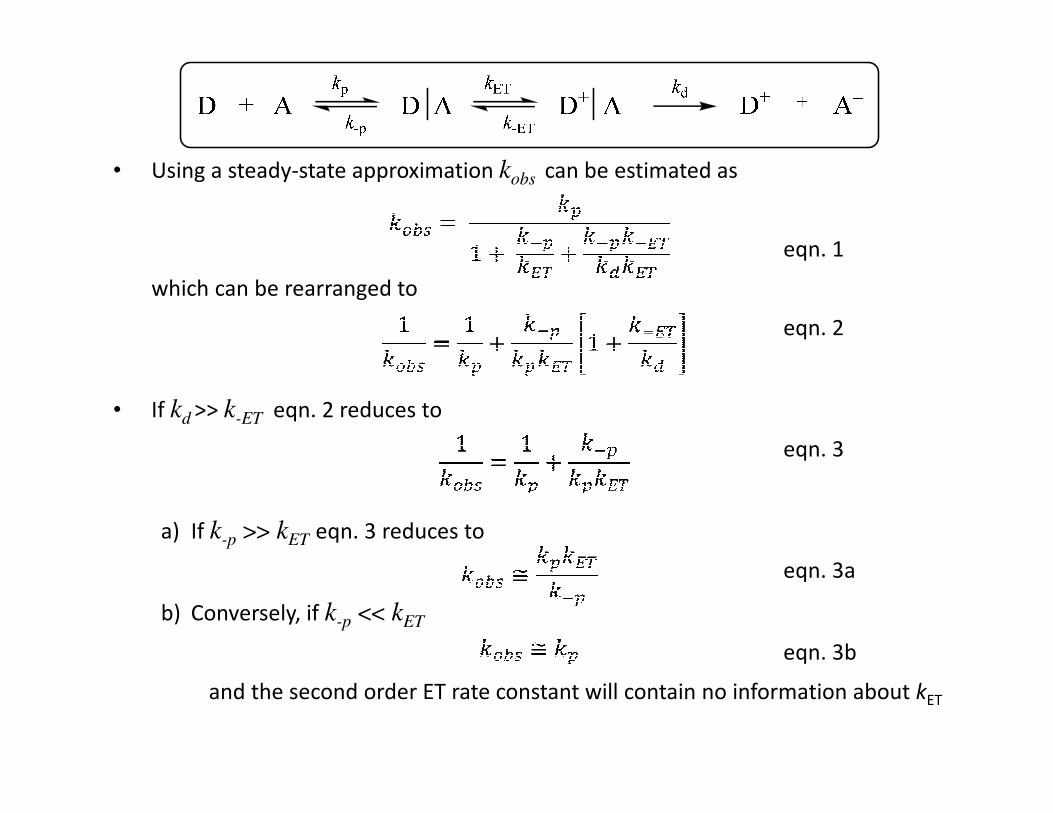
• Using a steady-state approximation kobs can be estimated as
eqn. 1
which can be rearranged to
eqn. 2
• If kd >> k-ET eqn. 2 reduces to
eqn. 3
a) If k-p >> kET eqn. 3 reduces to
eqn. 3a
b) Conversely, if k-p << kET
eqn. 3b
and the second order ET rate constant will contain no information about kET
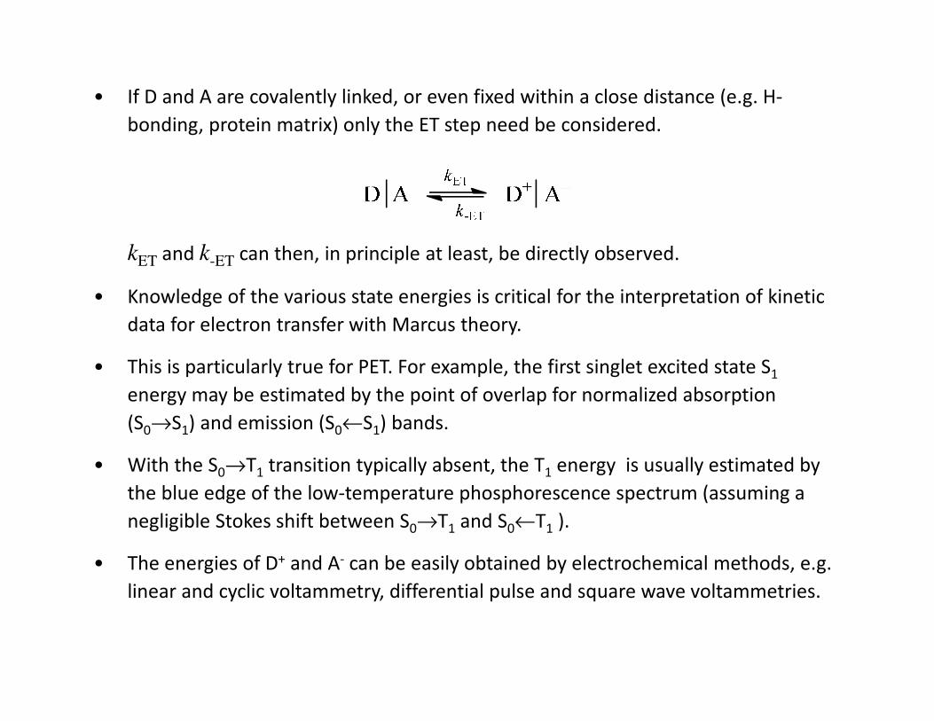
• If D and A are covalently linked, or even fixed within a close distance (e.g. H-
bonding, protein matrix) only the ET step need be considered.
kET and k-ET can then, in principle at least, be directly observed.
• Knowledge of the various state energies is critical for the interpretation of kinetic
data for electron transfer with Marcus theory.
• This is particularly true for PET. For example, the first singlet excited state S1
energy may be estimated by the point of overlap for normalized absorption
(S0→S1) and emission (S0←S1) bands.
• With the S0→T1 transition typically absent, the T1 energy is usually estimated by
the blue edge of the low-temperature phosphorescence spectrum (assuming a
negligible Stokes shift between S0→T1 and S0←T1 ).
• The energies of D+ and A- can be easily obtained by electrochemical methods, e.g.
linear and cyclic voltammetry, differential pulse and square wave voltammetries.
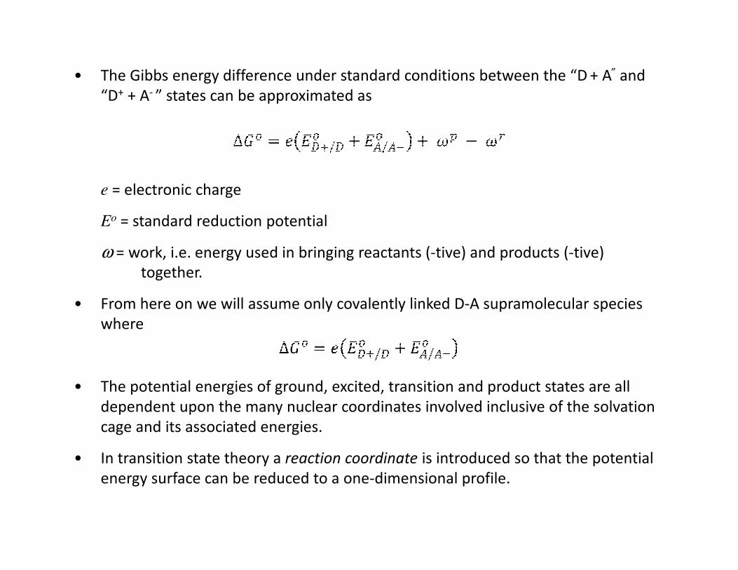
• The Gibbs energy difference under standard conditions between the “D + A” and “D+ + A- ” states can be approximated as
e = electronic charge
Eo = standard reduction potential
ω = work, i.e. energy used in bringing reactants (-tive) and products (-tive) together.
• From here on we will assume only covalently linked D-A supramolecular species where
• The potential energies of ground, excited, transition and product states are all dependent upon the many nuclear coordinates involved inclusive of the solvation cage and its associated energies.
• In transition state theory a reaction coordinate is introduced so that the potential energy surface can be reduced to a one-dimensional profile.

• Curve R represents the reactant stateDA while curve P represents theproduct state D+A-
• For ET to occur the reactant statemust distort from its equilibriumenergy state to reach a transitionstate geometry ‡ which also exists asa distorted form of the product state.
• Electron transfer occurs at the pointalong the reaction coordinate as thetransition state has a 50% probabilityof producing the D+A- product state(at least in this ideal symmetrical casewith ∆Go = 0)
[note: Marcus theory assumes R and Pcurves are of equal shape. This modelneglects external solvation effects,when included give a more accuratenon-parabolic picture]
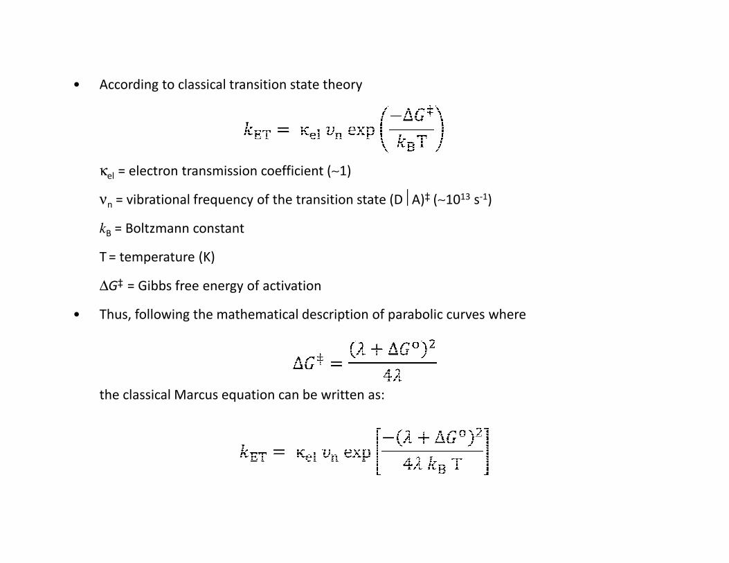
• According to classical transition state theory
κel = electron transmission coefficient (∼1)
νn = vibrational frequency of the transition state (DA)‡ (∼1013 s-1)
kB = Boltzmann constant
T = temperature (K)
∆G‡ = Gibbs free energy of activation
• Thus, following the mathematical description of parabolic curves where
the classical Marcus equation can be written as:
λ λλ
∆Go
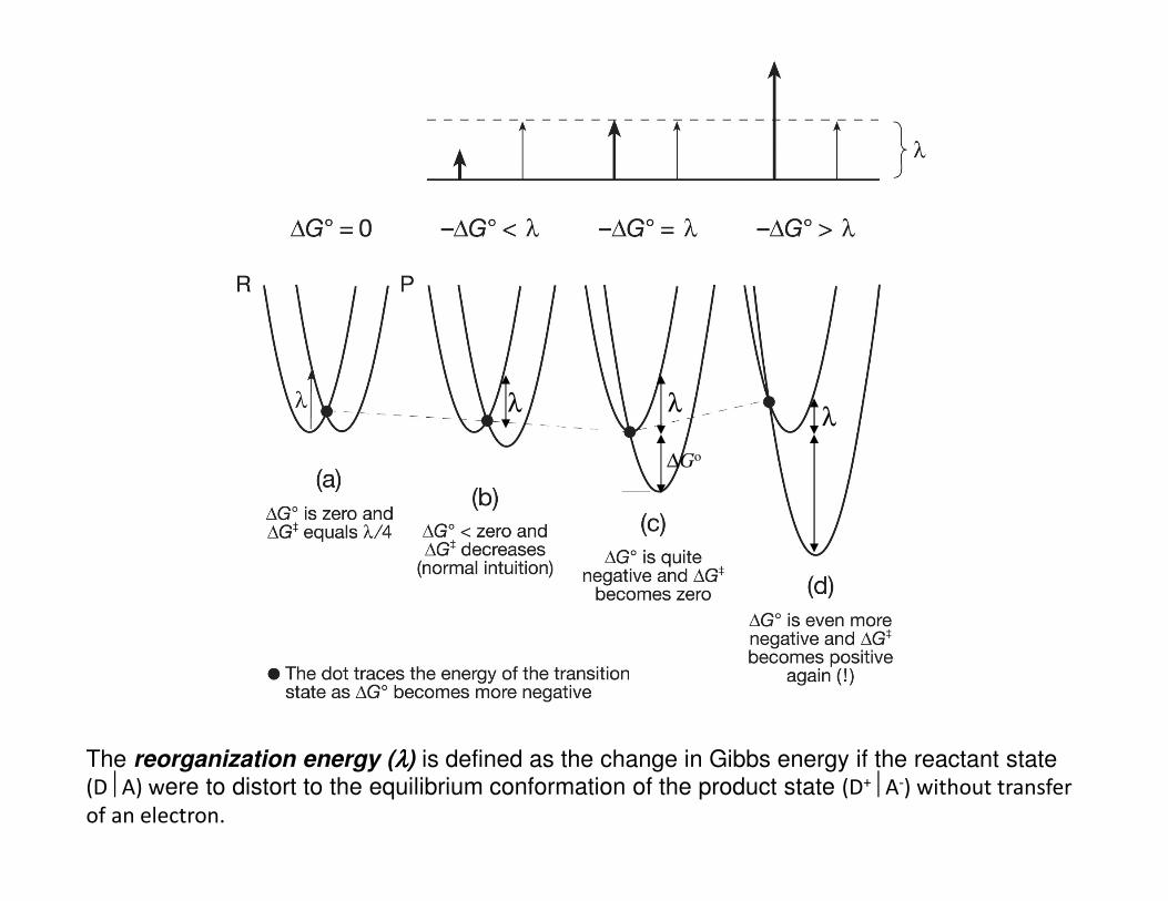
The reorganization energy (λλλλ) is defined as the change in Gibbs energy if the reactant state (DA) were to distort to the equilibrium conformation of the product state (D+A-) without transfer of an electron.
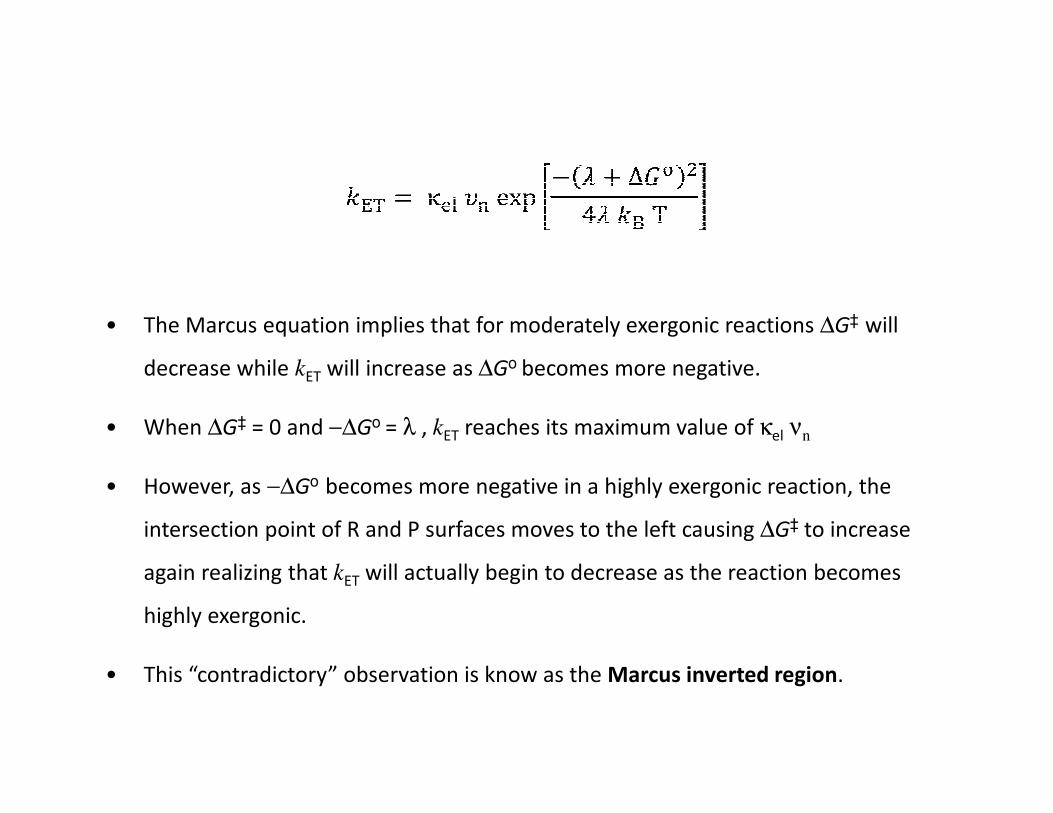
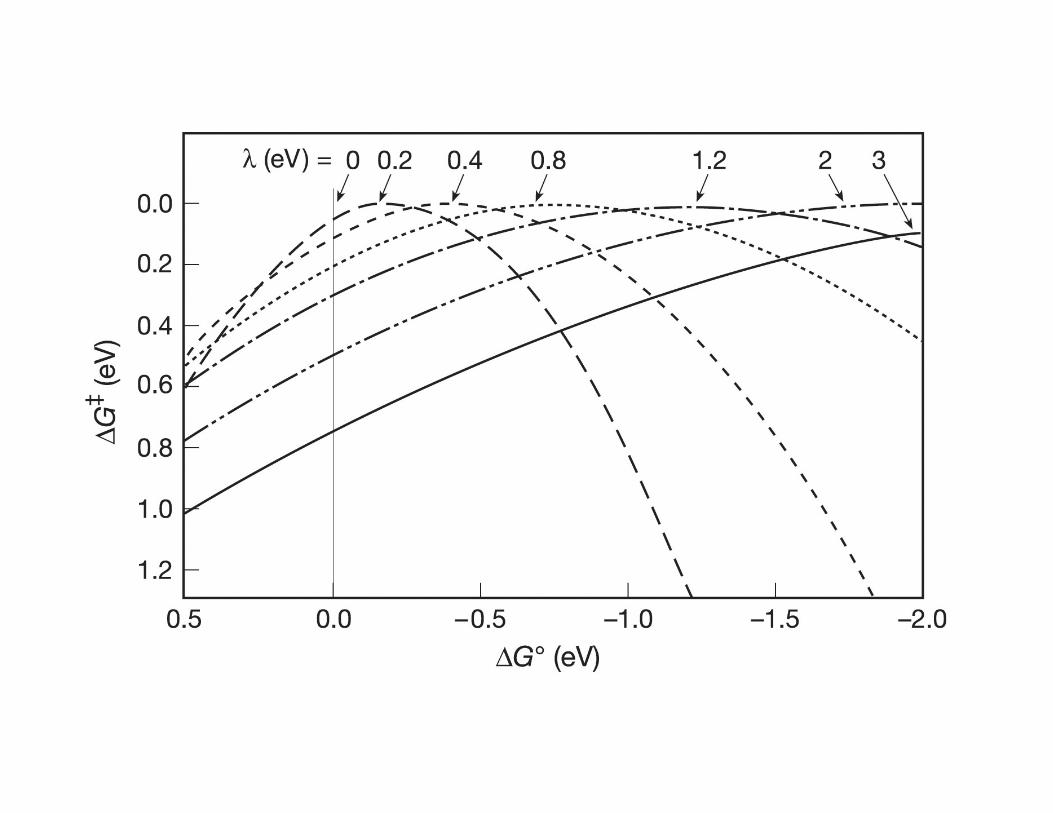
• The Marcus equation implies that for moderately exergonic reactions ∆G‡ will
decrease while kET will increase as ∆Go becomes more negative.
• When ∆G‡ = 0 and −∆Go = λ , kET reaches its maximum value of κel νn
• However, as −∆Go becomes more negative in a highly exergonic reaction, the
intersection point of R and P surfaces moves to the left causing ∆G‡ to increase
again realizing that kET will actually begin to decrease as the reaction becomes
highly exergonic.
• This “contradictory” observation is know as the Marcus inverted region.
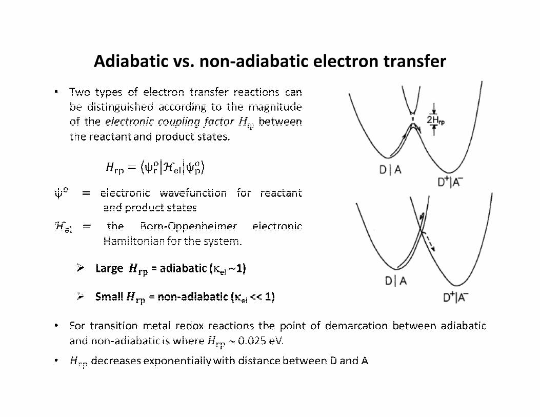
Adiabatic vs. non-adiabatic electron transfer
• Mixed-valence compounds contain an element which, at least in a formal sense,
exists in more than one oxidation state.
• This is a common phenomenon, e.g. Prussian blue which has a cyanide-bridged
Fe(II)-Fe(III) structure, was one of the first chemical materials to be described.
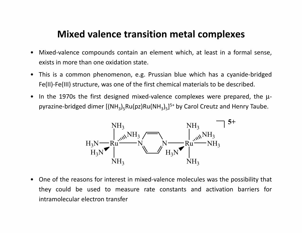
• In the 1970s the first designed mixed-valence complexes were prepared, the µ-
pyrazine-bridged dimer [(NH3)5Ru(pz)Ru(NH3)5]5+ by Carol Creutz and Henry Taube.
• One of the reasons for interest in mixed-valence molecules was the possibility that
they could be used to measure rate constants and activation barriers for
intramolecular electron transfer
Mixed valence transition metal complexes
Ru
NH3
NH3
H3N N
NH3
H3N
N Ru
NH3
NH3
NH3
H3N
NH3
5+

• These reactions have proven difficult to study by direct measurement, but the
analogous light-driven process can often be observed as a broad, solvent-
dependent absorption band.
• For symmetrical mixed-valence complexes these bands typically appear in low-
energy visible or near-infrared spectra.
• They are typically called intervalence transfer (IT), metal-metal charge transfer
(MMCT), or intervalence charge transfer (IVCT) bands.
• Hush provided an analysis of IT band shapes based on parameters that also define
the electron-transfer barrier.
• The barrier arises from nuclear motions whose equilibrium displacements are
affected by the difference in electron content between oxidation states.
• This includes both intramolecular structural changes and the solvent where there
are changes in the orientations of local solvent dipoles.
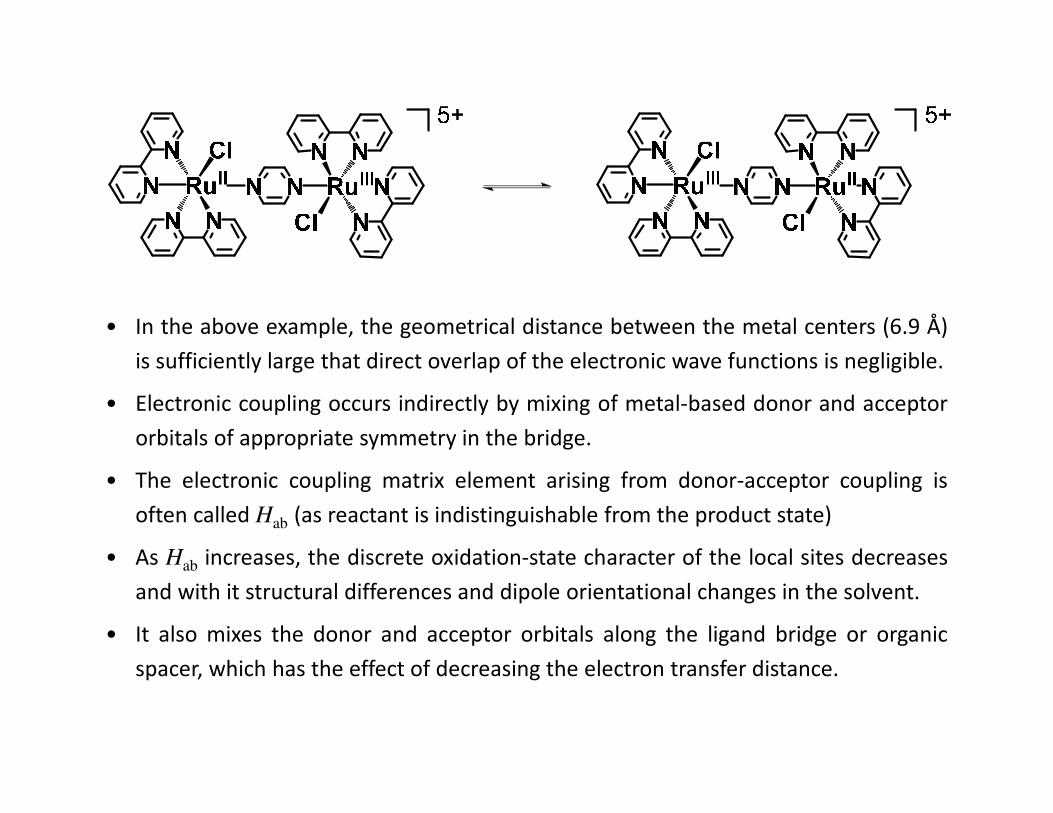
• In the above example, the geometrical distance between the metal centers (6.9 Å)
is sufficiently large that direct overlap of the electronic wave functions is negligible.
• Electronic coupling occurs indirectly by mixing of metal-based donor and acceptor
orbitals of appropriate symmetry in the bridge.
• The electronic coupling matrix element arising from donor-acceptor coupling is
often called Hab (as reactant is indistinguishable from the product state)
• As Hab increases, the discrete oxidation-state character of the local sites decreases
and with it structural differences and dipole orientational changes in the solvent.
• It also mixes the donor and acceptor orbitals along the ligand bridge or organic
spacer, which has the effect of decreasing the electron transfer distance.
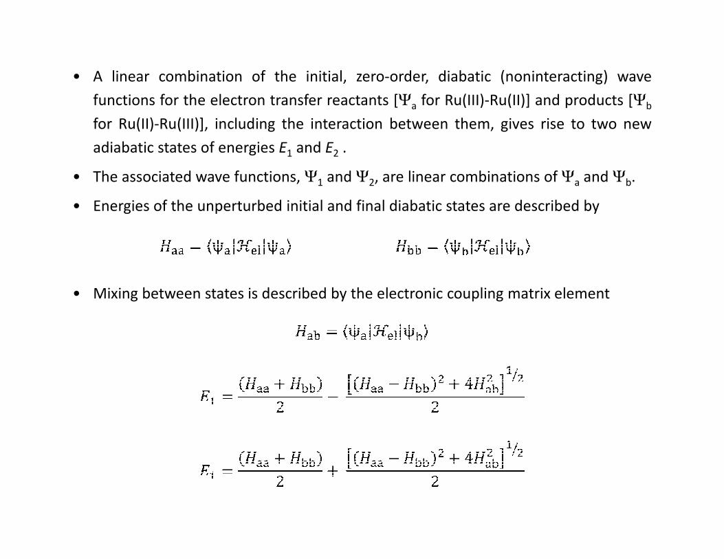
• A linear combination of the initial, zero-order, diabatic (noninteracting) wave
functions for the electron transfer reactants [Ψa for Ru(III)-Ru(II)] and products [Ψb
for Ru(II)-Ru(III)], including the interaction between them, gives rise to two new
adiabatic states of energies E1 and E2 .
• The associated wave functions, Ψ1 and Ψ2, are linear combinations of Ψa and Ψb.
• Energies of the unperturbed initial and final diabatic states are described by
• Mixing between states is described by the electronic coupling matrix element

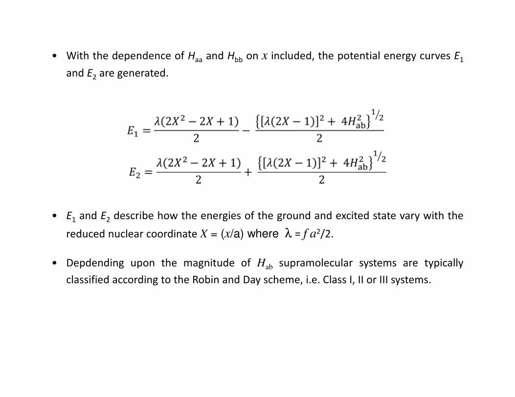
• With the dependence of Haa and Hbb on x included, the potential energy curves E1
and E2 are generated.
• E1 and E2 describe how the energies of the ground and excited state vary with the
reduced nuclear coordinate X = (x/a) where λ = f a2/2.
• Depdending upon the magnitude of Hab supramolecular systems are typically
classified according to the Robin and Day scheme, i.e. Class I, II or III systems.
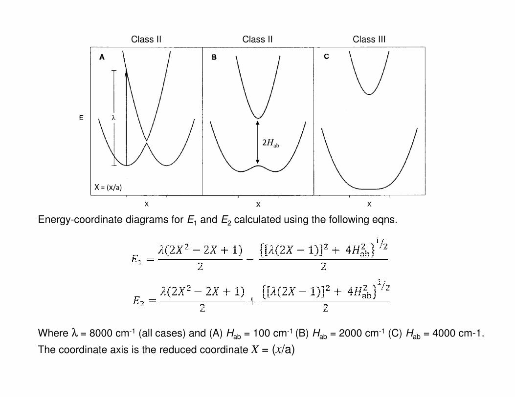
Energy-coordinate diagrams for E1 and E2 calculated using the following eqns.
Where λ = 8000 cm-1 (all cases) and (A) Hab = 100 cm-1 (B) Hab = 2000 cm-1 (C) Hab = 4000 cm-1.
The coordinate axis is the reduced coordinate X = (x/a)
X = (x/a)
2Hab
Class II Class II Class III
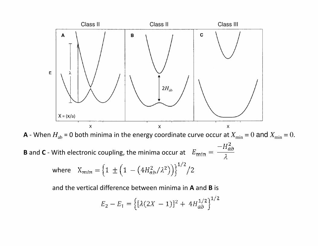
A - When Hab = 0 both minima in the energy coordinate curve occur at Xmin = 0 and Xmin = 0.
B and C - With electronic coupling, the minima occur at
where
and the vertical difference between minima in A and B is
X = (x/a)
2Hab
Class II Class II Class III
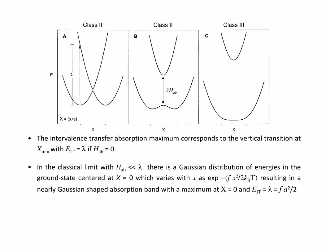
• The intervalence transfer absorption maximum corresponds to the vertical transition at
Xmin with EIT = λ if Hab = 0.
• In the classical limit with Hab << λ there is a Gaussian distribution of energies in the
ground-state centered at X = 0 which varies with x as exp −(f x2/2kBT) resulting in a
nearly Gaussian shaped absorption band with a maximum at X = 0 and EIT = λ = f a2/2
X = (x/a)
2Hab
Class II Class II Class III

X = (x/a)
2Hab
Class II Class II Class III


• The IT transition results in intramolecular electron transfer, e.g.,
Rua(II)-Rub(III) → {Rua(III)-Rub(II)}
• The electron-transfer product, {Rua(III)-Rub(II)}, formed in excited levels of the solvent
and vibrational modes coupled to the transition.
• Subsequent relaxation occurs to the intersection region at X = 1/2, where further
relaxation or intramolecular electron transfer give a distribution of Rua(II)-Rub(III) and
Rua(III)-Rub(II).
• In Class II there are localized valences (oxidation states) and measurable electronic
coupling ( Hab > 0 ).
• Class I is the limiting case with Hab = 0.
• Class III occurs when 2Hab2 /λ ≥ 1 and there is no longer a barrier to electron transfer
and the absorption band arises from a transition between delocalized electronic
levels (Ψa ± Ψb). Solvent coupling and λο is far less than for intervalence transfer since
there is no net charge transfer in the transition.

• The mixed-valence N2 bridged osmium compounds below show strong behavior
characteristic of Class II complexes.
Ligand bridged Osmium complexes
• Intense ν(N2) stretches appear at 2007 cm-1 for tpy
and 2029 cm-1 for tpm consistent with electronic
asymmetry on the time scale of the IR absorption
response (recorded in KBr pellets)

• IR-NIR spectra for a series of N2 bridged mixed valence osmium complexes
recorded in acetonitrile.

• Bands I and II provide an oxidation-state marker for Os(III).
• Due to low symmetry, extensive metal-ligand overlap, and spin-orbit coupling
[χ = 3 000 cm-1 for Os(III)] the d5 Os(III) core is split into three Kramer’s
doublets (E1’ , E2
’ , E3’ ) separated by thousands of cm-1.
E3’ = dπ1
1 dπ22 dπ3
2 (IC-2)
E2’ = dπ1
2 dπ21 dπ3
2 (IC-1)
E1’ = dπ1
2 dπ22 dπ3
1 (GS)

• Bands I (IC-1) and II (IC-2), are called
interconfigurational (IC) transitions, assigned to
transitions between the Kramer’s doublets.
• They are LaPorte forbidden but gain intensity
through spin-orbit coupling and M-L mixing.
• IC bands are less commonly observed for Fe(III),
χ ∼ 500 cm-1, or for Ru(III), χ ∼ 1000 cm-1.

• The remaining three bands (III, IV, V) can be
assigned to IT transitions arising from separate
electronic excitations across the bridge from the
three dπ orbitals at Os(II) to the hole at Os(III).
• These bands are also narrow but slightly
broader than the IC bands, which helps to
distinguish them in making band assignments.

• With weaker ligand field splitting in first and
second row transition metals the IT transitions
typically merge into a single broad overlapping
absorption band.
• Transitions IT-2 and IT-3 generate E2’ and E3
’
Kramer’s doublet configurations at the new
Os(III) center.

• Assuming the classical limit and a constant λ, the
energies of the IC and IT bands are related as
EIT (1) = λ
EIT (2) = ∆G1° + λ ≈ EIT (1) + λ
EIT (3) = ∆G2° + λ ≈ EIT (2) + λ

Energy-coordinate diagrams for E1 and E2
calculated using the following eqns.
λ = 7000 cm-1
Hab(1) = 118 cm-1
The upper two sets of curves were calculated similarly but offsetting by
EIC (1) = 3460 cm-1
EIC (1) = 5200 cm-1
with
Hab(2) = 723 cm-1
and Hab(3) = 595 cm-1