Marginal Treatment Effects and the External Validity of the

Oregon Health Insurance Experiment∗

Amanda E. KowalskiAssociate Professor, Department of Economics, Yale University

Faculty Research Fellow, NBER

August 13, 2015

Abstract

I examine the external validity of the Oregon Health Insurance Experiment (OHIE) usingmarginal treatment effect (MTE) methods. A central finding from the OHIE is that individ-uals who gained health insurance through the OHIE lottery increased their emergency roomutilization (Taubman et al. [2014]). Using data from the OHIE, I find that that the marginaltreatment effect of health insurance on emergency room utilization was positive for some typesof individuals and negative for others. Thus, the external validity of the finding that emergencyroom utilization increases when health insurance expands depends on the types of individualswho gain coverage. Using data from Kolstad and Kowalski [2012], I reexamine the types ofindividuals who gained coverage through the Massachusetts health reform, which established amandate for uninsured individuals to purchase coverage or pay a penalty, among other interven-tions. I find that the Massachusetts individuals induced to gain health insurance appear moresimilar to the Oregon individuals that decreased their emergency room utilization than they doto the Oregon individuals that increased their emergency room utilization. Furthermore, on thewhole, individuals who entered a lottery for health insurance coverage in Oregon likely had ahigher desire to use the emergency room than individuals who gained coverage when a mandaterequired them to do so in Massachusetts. Therefore, it is not surprising that that literature findsdecreases in emergency room utilization in Massachusetts despite increases in Oregon becausethe two state policy interventions expanded coverage to different types of individuals. Giventhat my findings deepen our understanding of the external validity of the OHIE, I conclude thatMTE methods are a valuable addition to the standard toolkit for analysis of experiments andquasi-experiments with binary treatments. Based on my analysis, I highlight several researchdesign considerations that can maximize the ability of MTE methods to shed light on externalvalidity in future applications.

∗Preliminary. Comments very welcome. I thank Aigerim Kabdiyeva and especially Samuel Moy for excellentresearch assistance. I also thank Ashley Swanson for a helpful conference discussion. Joseph Altonji, Steve Berry,Lasse Brune, Amy Finkelstein, Magne Mogstad, Costas Meghir, Joseph Shapiro, Ed Vytlacil, and seminar participantsat Yale and the WEAI provided helpful comments.

1

1 Introduction

A central finding from the Oregon Health Insurance Experiment (OHIE) is that individuals who

gained health insurance through the OHIE lottery increased their emergency room utilization

(Taubman et al. [2014]). This finding has attracted considerable interest because legislation re-

quires that emergency rooms see all patients, regardless of whether they have health insurance,

making the emergency room the main portal through which the uninsured enter the healthcare

system. The emergency room utilization of the uninsured places a burden on other players in the

healthcare system, including insured patients who face long wait times in the emergency room and

hospitals that provide uncompensated care. Care provided through emergency rooms also likely

costs more to provide than care in other settings. Furthermore, the uninsured themselves could

potentially get better continuity of care and better quality of care through other outlets. For these

reasons, policymakers hope that expansions of health insurance coverage to the uninsured will de-

crease emergency room utilization. The finding that emergency room utilization increased when

the uninsured in the OHIE gained coverage caused a stir because it incited fears that the national

coverage expansions currently underway through the implementation of the Affordable Care Act

(ACA) would also increase emergency room utilization and therefore cost.

Relative to the other evidence on the impact of expanding health insurance coverage on emer-

gency room utilization, the OHIE evidence is the “gold standard” because it is based on a ran-

domized controlled trial (RCT) and because it took place recently in 2008. Another main source

of evidence is based on quasi-experimental variation from the Massachusetts health reform of 2006.

That literature finds that emergency room visits decreased (Miller [2012], Smulowitz et al. [2011])

or stayed the same (Chen et al. [2011]), and admissions to the hospital from the emergency room

(a proxy for emergency room visits) decreased (Kolstad and Kowalski [2012]). Without formal

tools to reconcile the conflicting results from Oregon and Massachusetts, or any two studies for

that matter, readers might simply choose to place more weight on results from RCTs. As an al-

ternative, they might note that it is hard to generalize from either source of evidence because they

are both based on specific populations, and related evidence on the emergency room utilization

of other populations of newly insured individuals also yields conflicting results (see Currie and

Gruber [1996],Anderson et al. [2012], Anderson et al. [2014], and Newhouse and Rand Corporation

2

Insurance Experiment Group [1993]).

In this paper, I use a data-driven approach based on recently developed econometric methods

to say more about the external validity of the results from the OHIE. Specifically, I use marginal

treatment effect (MTE) methods introduced by Bjorklund and Moffitt [1987] and generalized by

Heckman and Vytlacil [1999] and Heckman and Vytlacil [2005] and Heckman and Vytlacil [2007].

Until recently, identification issues hindered the use of MTE methods in empirical settings with

binary instruments. Hence, these methods could not be applied to RCT’s that utilize binary

assignment to a lottery, such as the OHIE. The extensions developed in Brinch et al. [2012] for

discrete instruments allow me add marginal treatment effect estimation to the set of tools available

for analysis of RCT’s.

The key innovation of using MTE methods to analyze experiments is that they glean information

from empirical selection into treatment. Even if subjects are randomized into a treatment or a

control group to evaluate the outcome of an intervention, unless all participants randomized into

the treatment group receive the intervention (and all participants randomized into the control group

do not receive the intervention), then selection into receipt of the intervention (sometimes called

“attendance” or “takeup”) will influence the external validity of the results obtained. External

validity is an issue even if the data are analyzed within an instrumental variables “intent-to-treat”

framework, which only addresses internal validity. MTE methods expand the toolkit available to

address external validity.

I revisit the results of the OHIE using marginal treatment effect methods. Using data from

the OHIE, I find that that the marginal treatment effect of health insurance on emergency room

utilization was positive for some types of individuals and negative for others. Thus, the external

validity of the finding that emergency room utilization increases when health insurance expands

depends on the types of individuals who gain coverage.

Using data from Kolstad and Kowalski [2012], I reexamine the types of individuals who gained

coverage through the Massachusetts health reform, which established a mandate for uninsured

individuals to purchase coverage or pay a penalty, among other interventions. I find that the Mas-

sachusetts individuals induced to gain health insurance appear more similar to the Oregon individ-

uals that decreased their emergency room utilization than they do to the Oregon individuals that

increased their emergency room utilization. Furthermore, on the whole, individuals who entered a

3

lottery for health insurance coverage in Oregon likely had a higher desire to use the emergency room

than individuals who gained coverage when a mandate required them to do so in Massachusetts.

Therefore, it is not surprising that that literature finds decreases in emergency room utilization

in Massachusetts despite increases in Oregon because the two state policy interventions expanded

coverage to different types of individuals. Given that my findings deepen our understanding of the

external validity of the OHIE, I conclude that MTE methods will be a valuable addition to the

standard toolkit for analysis of experiments and quasi-experiments with binary treatments. Based

on my analysis, I highlight several research design considerations that can maximize the ability of

MTE methods to shed light on external validity in future applications.

In the next section, I present the generalized Roy model that forms the foundation for MTE

methods, and I discuss marginal treatment effects in Section 3. In Section 4, I replicate results

from the OHIE, and I extend them to allow for the application of MTE methods. I present the

MTE results in Section 5. I discuss the implications of the results for the reconciliation of the

Oregon and Massachusetts results in Section 6. In Section 7, I compare my results with results

from standard analysis of treatment effect heterogeneity. I explore the robustness of the results in

Section 8; I discuss the broader implications of my findings for experimental design in Section 9;

and I conclude in Section 10.

2 Model

Let Y be the observed outcome of interest, emergency room utilization. Let D represent the

binary treatment of interest, health insurance coverage. Define Y1 as the potential outcome of an

individual in the treated state (D = 1), and define Y0 as the potential outcome of an individual

in the untreated state (D = 0), such that Y1 represents potential emergency room utilization with

health insurance coverage, and Y0 represents potential emergency room utilization without health

insurance coverage. The following model relates the potential outcomes to the observed outcome:

Y = (1−D)Y0 +DY1.

4

I specify the potential outcomes as follows

Y1 = µ1(X) + U1

Y0 = µ0(X) + U0,

where µ1() and µ1() are general functions, and X is a random vector of covariates such as age and

gender. U1 and U0 are random variables that are normalized such that E(U1|X = x) = E(U0|X =

x) = 0. I assume that E(U2j |X = x) exists for j = 0, 1 for all x in the support of X, but we do not

assume independence between X and (U0, U1).

In this model, an individual selects into treatment D (health insurance coverage) based on the

net benefit of treatment, ID, which we specify as follows:

ID = µD(W )− UD

where µD() is a general function of W = (X,Z) where Z represents the excluded instrument(s).

In the OHIE context, Z is a variable that indicates winning a health insurance lottery. We can

interpret µD(W ) as the observed benefit of treatment. UD is a random variable, which we can

interpret as the unobserved cost of treatment. An individual selects into treatment of the observed

benefit of treatment exceeds the unobserved cost of treatment, yielding a positive net benefit:

D = 1{ID > 0} ⇐⇒ µD(W ) > UD.

We assume that UD is continuous with a cumulative distribution function FUD() that is strictly

increasing. Therefore, the quantiles of UD are uniformly distributed. Define P (W ) ≡ Pr(D =

1|W ) = FUD(µD(W )). This normalization allows us to interpret P (W ) as a propensity score. If

µD(W ) is a propensity score, then P (W ) is a uniformly distributed propensity score. An individual

selects into treatment if P (W ) exceeds the quantile of the unobserved cost of treatment UD.

Now, suppose that under this model, we specify the following standard regression model for

estimation

Y = σ + βD +X ′δ + ε (1)

5

D = φ+ γZ +X ′θ + ν, (2)

where Y , D, and Z are defined as above, σ and φ are constant terms, β and γ are coefficients, and

ε and ν are error terms. If we estimate Equation (1) via ordinary least squares (OLS), then our

estimate will be affected by selection bias because the treatment D (health insurance) is correlated

with the error ε conditional on the covariates X. To address this selection bias, suppose that we

follow the standard practice of estimating Equations (1) and (2) using an instrumental variable

(IV) estimator. If β is a fixed coefficient, then IV recovers the true β and overcomes selection bias.

However, if β is a random coefficient, then IV recovers a local average treatment effect (LATE),

as introduced by Imbens and Angrist [1994], because under the generalized Roy model, the treat-

ment D is correlated with the gains from treatment β. In the OHIE context, even though individuals

win or lose the lottery, they can still decide whether to take up health insurance, and they will make

the decision of whether to take up health insurance based on their net benefit. Thus, individuals

would benefit most from health insurance, perhaps through emergency room utilization, are likely

to follow through and sign up for health insurance.

Once we move from a world where β is fixed to a world where β can be random, in general,

different experiments generally estimate different LATEs. In this world, there is no problem with

internal validity, but there is no guarantee of external validity. Different experiments or policies,

which manifest themselves as different definitions of the instrument Z will recover different LATEs.

3 Marginal Treatment Effects

Rather than simply concluding that the results from OHIE do not necessarily generalize, I compute

marginal treatment effects (MTE) in attempt to say more about external validity. We begin with

the definition of the MTE:

Definition 1. The MTE is the average treatment effect for individuals with covariate values X = x

and an unobserved component of the net benefit of treatment of UD = p:

MTE(x, p) = E(Y1 − Y0|X = x, UD = p).

In the context of the OHIE, we are interested in the treatment effect of health insurance on emer-

6

gency room utilization. Each individual has a treatment effect. We average the treatment effects

over all individuals with the same realized observed characteristics x and unobserved characteristics

p (for example, young women with a high unobserved component of the net benefit of treatment)

to compute an MTE. We can calculate a different marginal treatment effect for each combination

of observed and unobserved characteristics, resulting in an MTE function.

If the outcome Y is specified in dollars, then the MTE has a convenient interpretation as the

willingness to pay for treatment for individuals at the margin of indifference between selecting into

treatment and not selecting into treatment. In the OHIE context, the MTE can be interpreted as

the willingness to pay for health insurance for individuals at the margin of signing up for health

insurance vs. going uninsured. We infer that individuals with high observed benefits of insurance

who are at the margin of gaining coverage must have high unobserved costs.

Any local average treatment effect (LATE) can be recovered as an integral of a marginal treat-

ment effect function. Following Heckman and Vytlacil [1999] and Heckman and Vytlacil [2005] and

Heckman and Vytlacil [2007], we can calculate the LATE for a given binary instrument (Z ∈ 0, 1)

as follows:

LATE(x) =E(Y |Z = 1, X = x)− E(Y |Z = 0, X = x)

E(D|Z = 1, X = x)− E(D|Z = 0, X = x)

=1

p1(x)− p0(x)

∫ p1

p0

MTE(x, p)dp.

where the limits of integration result because the instrument Z shifts the propensity score of

receiving treatment from p0(x) = P (X = x, Z = 0) to p1(x) = P (X = x, Z = 1).

Just as we can recover the LATE from any experiment using an integral of the MTE, we can

recover other parameters of interest as weighted averages of the MTE. These parameters include

the average treatment effect (ATE), the average treatment effect on the untreated (ATUT), and

the average treatment effect on the treated (ATT). We include the formulas for these parameters

in Appendix A, following Heckman and Vytlacil [2007]. As we can see from the formulas, the ATT

is distinct from what the experimental literature calls the “treatment on the treated,” which is

actually just a LATE.

7

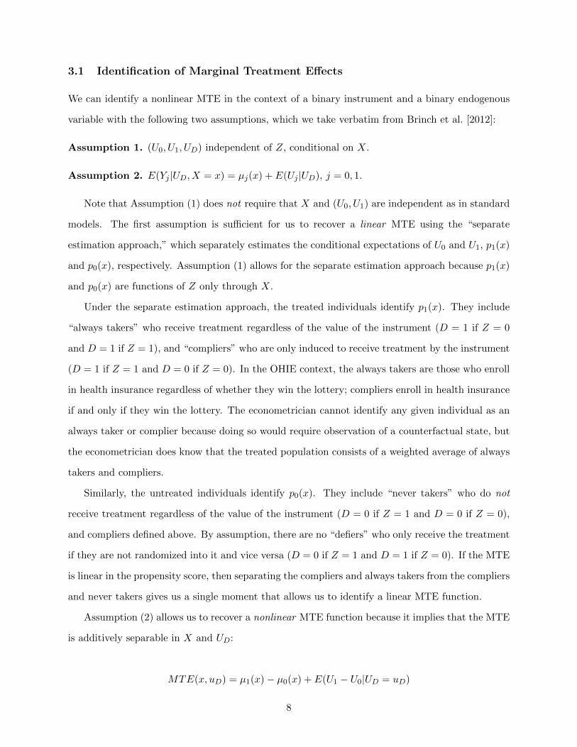
3.1 Identification of Marginal Treatment Effects

We can identify a nonlinear MTE in the context of a binary instrument and a binary endogenous

variable with the following two assumptions, which we take verbatim from Brinch et al. [2012]:

Assumption 1. (U0, U1, UD) independent of Z, conditional on X.

Assumption 2. E(Yj |UD, X = x) = µj(x) + E(Uj |UD), j = 0, 1.

Note that Assumption (1) does not require that X and (U0, U1) are independent as in standard

models. The first assumption is sufficient for us to recover a linear MTE using the “separate

estimation approach,” which separately estimates the conditional expectations of U0 and U1, p1(x)

and p0(x), respectively. Assumption (1) allows for the separate estimation approach because p1(x)

and p0(x) are functions of Z only through X.

Under the separate estimation approach, the treated individuals identify p1(x). They include

“always takers” who receive treatment regardless of the value of the instrument (D = 1 if Z = 0

and D = 1 if Z = 1), and “compliers” who are only induced to receive treatment by the instrument

(D = 1 if Z = 1 and D = 0 if Z = 0). In the OHIE context, the always takers are those who enroll

in health insurance regardless of whether they win the lottery; compliers enroll in health insurance

if and only if they win the lottery. The econometrician cannot identify any given individual as an

always taker or complier because doing so would require observation of a counterfactual state, but

the econometrician does know that the treated population consists of a weighted average of always

takers and compliers.

Similarly, the untreated individuals identify p0(x). They include “never takers” who do not

receive treatment regardless of the value of the instrument (D = 0 if Z = 1 and D = 0 if Z = 0),

and compliers defined above. By assumption, there are no “defiers” who only receive the treatment

if they are not randomized into it and vice versa (D = 0 if Z = 1 and D = 1 if Z = 0). If the MTE

is linear in the propensity score, then separating the compliers and always takers from the compliers

and never takers gives us a single moment that allows us to identify a linear MTE function.

Assumption (2) allows us to recover a nonlinear MTE function because it implies that the MTE

is additively separable in X and UD:

MTE(x, uD) = µ1(x)− µ0(x) + E(U1 − U0|UD = uD)

8

Given this additive separability, we have an additional moment within each x. For example, in the

OHIE context, we can estimate a propensity score for treated women and untreated women and a

propensity score for treated men and untreated men. By assumption, the MTE for women should

be the same regardless of whether they win the lottery or not, and the MTE for men should be

the same regardless of whether they win the lottery or not. We can use this assumption to fit a

nonlinear MTE to the propensity scores from both genders in a pooled specification.

Assumptions (1) and (2) are weaker than assumptions required by many standard models.

However, they are harder to defend if the outcome Y is binary or discrete. Extending MTE

estimation to contexts with binary instruments and binary dependent variables is an important

area for future work. Here, we always report estimates with Y specified as a number of visits

alongside Y specified as a binary variable for any visits to assess the sensitivity of the results to

the specification of the dependent variable.

3.2 Estimation of Marginal Treatment Effects

To estimate the MTE, we specify the following functional form:

MTE(x, p) = E(Y1 − Y0|X = x, UD = p) = (β1 − β0)′x+ k(p). (3)

We detail our MTE estimation algorithm in Appendix B. We also intend to make our Stata

code available for use in other applications.

As we can see from Equation (3), the MTE function does not vary with the instrument Z.

Therefore, the MTE should not vary across repeated experiments. In practice, if the MTE varies

across experiments, then we can conclude, in the spirit of a Hausman [1978] test, that one of the

experiments is invalid or that an assumption required for MTE estimation is violated. However, the

MTE does vary with the outcome variable Y , the endogenous variable D, and the set of covariates

X. The MTE function will also vary with a set of ancillary estimation parameters: the functional

form for k(p) (local linear in the base case), the estimation grid P with associated bandwidth h

(0.1 in the base case), as discussed in Appendix B. In our application to the OHIE, we demonstrate

how the MTE varies with different modeling choices.

9

4 Bringing MTE to the OHIE

4.1 Replication and Extension

To estimate marginal treatment effects in the OHIE, we first replicate the main IV results reported

in Taubman et al. [2014]. We then extend them to allow for MTE estimation, showing that our

extensions leave the main findings intact. Our dependent variable of interest Y is emergency room

utilization. Following Taubman et al. [2014], we specify emergency room utilization in two ways.

The top panel of Table 1 reports impacts on the probability of having any emergency room visit,

and the bottom panel reports impacts on the number of emergency room visits, including zeroes

for individuals with no visits.

Using the publicly available data, we replicate the main results from Taubman et al. [2014] in

Column (1). We use the full set of administrative data available on 24,646 lottery entrants. The

coefficient in the top panel of Column (1), which we replicate exactly, indicates that individuals

who receive Medicaid coverage increase the probability that they visit the emergency room by 6.97

percentage points on a base of 34 percentage points in the control group (a 20.5% increase). The

coefficient in the bottom panel indicates that individuals who receive Medicaid coverage increase

their visits to the emergency room by 0.387 visits on a base of 1.00 visit in the control group (a

38.7% increase). As detailed in the table notes, we cannot replicate the result in the bottom panel

exactly because of censoring and truncation performed to limit the identification of human subjects

in the publicly-available data, but our estimate is very similar to the coefficient of 0.41 on a base

of 1.02 visits reported in Taubman et al. [2014].

Both estimates are statistically significant at the 1% level. Following Taubman et al. [2014], we

calculate standard errors clustered by household ID, which we report beneath each point estimate.

We report significance crosses on those standard errors. For comparison to the results from our MTE

methods, which require bootstrapped standard errors, we report standard errors block bootstrapped

by household ID with corresponding significance stars as the second set of errors. In practice, both

sets of standard errors differ very slightly.

Taubman et al. [2014] specifies the endogenous variable D as an indicator for any Medicaid

coverage, which includes Medicaid coverage obtained via the lottery and Medicaid coverage obtained

via existing eligibility guidelines. To examine the external validity of the OHIE, we re-specify

10

Table 1: OHIE Replication and Extension

Any  Emergency  Room  Visits(1) (2) (3) (4) (5) (6) (7)

Medicaid 0.0697(0.024)†††  (0.024)***

Any  insurance 0.0610 0.0665 -­‐0.0124 0.0638 0.207 0.0453(0.021)††† (0.023)††† (0.022) (0.022)††† (0.087)†† (0.023)††  (0.021)***  (0.023)*** (0.022)  (0.022)***  (0.094)**  (0.022)**

Control  variablesLottery  Entrants,

Pre-­‐VisitsLottery  Entrants,

Pre-­‐VisitsLottery  Entrants No  Controls

Lottery  Entrants,  Common  Controls

Common  Controls

Common  Controls

Regression  sampleFull  sample Full  sample Full  sample Full  sample Full  sample

2+  Lottery  Entrants

1  Lottery  Entrant

Observations 24,646 24,646 24,646 24,646 24,646 5,003 19,643R-­‐squared 0.151 0.146 0.023 0.036 0.050 0.033 0.033Mean  of  Y  in  control  group 0.34 0.34 0.34 0.34 0.34 0.21 0.37

Number  of  Emergency  Room  Visits(1) (2) (3) (4) (5) (6) (7)

Medicaid 0.387(0.107)†††(0.114)***

Any  insurance 0.339 0.300 -­‐0.0405 0.299 0.857 0.227(0.094)††† (0.115)††† (0.114) (0.114)††† (0.318)††† (0.123)†(0.100)*** (0.123)** (0.122) (0.122)**  (0.312)***  (0.129)*

Control  variablesLottery  Entrants,

Pre-­‐VisitsLottery  Entrants,

Pre-­‐VisitsLottery  Entrants No  Controls

Lottery  Entrants,  Common  Controls

Common  Controls

Common  Controls

Regression  sampleFull  sample Full  sample Full  sample Full  sample Full  sample

2+  Lottery  Entrants

1  Lottery  Entrant

Observations 24,615 24,615 24,622 24,622 24,622 5,000 19,622R-­‐squared 0.339 0.335 0.016 0.021 0.033 0.004 0.022Mean  of  Y  in  control  group 1.00 1.00 1.00 1.00 1.00 0.45 1.09†††  p<0.01,  ††  p<0.05,  †  p<0.1,  standard  errors  clustered  at  the  household  ID  level***  p<0.01,  **  p<0.05,  *  p<0.1,  standard  errors  block  bootstraped  at  the  household  ID  level

 "Lottery  Entrants"  indicates  the  number  of  lottery  entrants  in  the  Oregon  experiment  within  a  given  household.  Pre-­‐Visits  refers  to  any  ER  visits  in  the  pre-­‐period  and  number  of  ER  visits  in  the  pre-­‐period  in  the  top  and  bottom  specifications,  respectively.  Common  controls  are  gender,  English  speaker,  and  indicator  variable  for  each  age.  All  two-­‐way  interactions  between  control  variables  are  also  included.  Column  (1)  replicates  the  main  findings  regarding  ER  usage  in  Taubman  et  al  (2014).

Our  results  for  Number  of  ER  Visits  deviate  slightly  from  the  published  version  because  of  censoring  and  truncation  of  the  dependent  variable.  The  publicly  available  Oregon  documentation  files  states  in  ohie_userguide.pdf  on  page  7:"Most  continuous  variables  (e.g.  that  capture  the  total  number  of  ED  visits  in  a  given  period)  have  been  censored  to  ensure  de-­‐identification.  Variables  were  censored  so  that  no  individual  value  has  fewer  than  ten  observations.  This  results  in  the  right  tail  of  the  distribution  of  these  variables  being  grouped  into  one  large  upper  bin.  Consequently,  certain  results  reported  in  Taubman  et  al  (2014)  cannot  be  replicated  with  the  publicly  available  data  (for  a  list  of  replicable  analyses,  see  note  at  the  top  of  the  replication  code:  oregonhie_science_replication.do)."

The  details  for  the  censoring  and  truncation,  stated  in  oregonhie_ed_codebook.pdf  on  page  1,  are  as  follows:"This  variable  was  truncated  at  2*  99th  percentile  of  the  original  distribution  (conditional  on  being  non-­‐zero).  The  public  use  variable  was  additionally  censored  to  ensure  de-­‐identification  (see  User  Guide  for  explanation)."

To  obtain  the  bootstrapped  standard  errors,  we  block  bootstrap  by  household  ID  for  200  replications,  and  we  report  the  standard  deviation  of  the  replications  as  an  estimate  of  the  standard  error.  

11

the endogenous variable as “any health insurance coverage” because other contexts such as the

Massachusetts health reform and the Affordable Care Act expand other types of coverage as well

as Medicaid coverage. Respecifying the endogenous variable to make it narrower could result

in a violation of the exclusion restriction if the lottery affects outcomes outside of the narrower

endogenous variable. However, respecifying the endogenous variable to make it broader should

not induce new concerns about exclusion restriction violations. Empirically, when we change the

endogenous variable from Medicaid in Column (1) to any insurance in Column (2), the regression

coefficients change very little.

We next examine robustness of the OHIE results to the inclusion of control variables. To

examine the external validity of the OHIE for other contexts, we want to include only controls that

will be widely available in other contexts. Beyond that consideration, we want to include as many

controls as possible so that we can generalize our results to other populations in as much detail as

possible. Empirically, the more controls we include, the more finely we can estimate the nonlinear

MTE function via Assumption (2).

The main results in Taubman et al. [2014] include only two controls. The first is a control

for previous emergency room utilization, specified as noted in the table notes. In other empirical

contexts, we cannot construct control variables for previous emergency room utilization unless we

have longitudinal data, so we omit them from our extension of the OHIE results. When we do so in

Column (3) the R-squared values decrease, as expected, but the point estimates and the standard

errors remain almost unchanged from the previous column.

The second control included in the main OHIE results is a count of the number of lottery entrants

in the household. As noted in Taubman et al. [2014], the results are not robust to the removal of

this control. Indeed, when we further remove this control in Column (4), the coefficients become

negative and lose their statistical significance. This control is important because the OHIE allowed

multiple members of the same household to sign up for the health insurance lottery independently.

However, if any member of the household won the lottery, then all members of the household

were treated as winners. Thus, individuals in households with multiple entrants had a higher

probability of winning. The overall probability of winning the lottery was 39%, but the probability

of winning was 57% for individuals in households with multiple lottery entrants, in contrast to 34%

for individuals in households with a single lottery entrant.

12

As we try to draw conclusions about the external validity of the Oregon Health insurance

experiment, it is hard to specify a different covariate available in other contexts that would capture

the same information as the number of lottery entrants. Household size is the best candidate, but it

is not available in the administrative data. Furthermore, household size is distinct from the number

of lottery entrants because even if a household had two or more members, not all members signed

up for the lottery. It is possible that individuals who really wanted health insurance encouraged the

other members of their household to sign up for the lottery. It is also possible that these individuals

really wanted to visit the emergency room for care. The control for the number of lottery entrants

ensures that the OHIE results are internally valid because the results compare individuals who won

the lottery to individuals who did not win the lottery, conditional on the number of lottery entrants.

However, the control for the number of lottery entrants poses challenges for external validity.

To maximize what we can learn about external validity, we include the widest set of controls

that are available in the Oregon administrative data that are likely to be available in other contexts,

and we refer to them as the “common controls” in Table 1. These controls include an indicator

for gender, an indicator for English speakers, an indicator for each year of age, and all two-way

interactions. As we demonstrate in Column (5), the inclusion of the common controls alongside the

control for the number of lottery entrants leaves the coefficients virtually unchanged, so we retain

these common controls in the subsequent specifications.

In the last two columns, rather than control for the number of lottery entrants in the full sample,

we split the sample by the number of lottery entrants. As shown in Column (6), about 20% of the

sample had one more lottery entrant (only 0.21% of the sample had three lottery entrants, which

is the maximum value). Within the subsample with multiple lottery entrants, the mean emergency

room utilization in the control group is smaller than it is in the full sample, but the coefficients

are much larger. The coefficients indicate that obtaining health insurance coverage increases the

probability of an emergency room visit by 21 percentage points beyond the 21% visit rate in the

control group; it increases the number of visits by 0.86 visits beyond the 0.45 visits made in the

control group. Both estimates are statistically significant at at least the 5% level. Individuals who

were part of a household with multiple lottery entrants might have had some pent up demand for

emergency room care, which was available but not necessarily free.

In the last column, we report the same specification using only the 80% individuals who were

13

part of households with a single lottery entrant. The coefficients are still positive and statistically

significant at at least the 10% level, but their magnitudes are smaller, indicating that insurance

increases the probability of an emergency room visit by 4.53 percentage points on a base of 37

percentage points and that insurance increases the number of visits by 0.22 on a base of 1.09 visits.

We retain the specification in Column (7) as our preferred specification for the examination of

external validity using marginal treatment effects. Absent richer demographic information in the

administrative data, it is hard to identify which individuals in other contexts would resemble the

OHIE participants from households with multiple lottery entrants. Therefore, it seems reasonable

to examine the external validity using the sample of individuals with only a single lottery entrant.

We also report the robustness of our results to MTE specifications based on the full sample following

Column (5) and the sample with two or more lottery entrants following Column (6).

4.2 Statistics on Compliers, Always Takers, and Never Takers

MTE estimation for a binary instrument relies on the separation of compliers from always takers

and never takers through the separate estimation approach, made possible by Assumption (1).

Following Imbens and Angrist [1994], compliers identify the LATE estimated by IV. Although it

is not possible to identify compliers at the individual level, it is possible to identify their average

characteristics. This exercise can be implemented in all experimental or IV settings for which the

endogenous variable and the instrument are available for the same individual. It has not yet become

part of the standard toolkit, but it has been implemented for the OHIE.1

We calculate the average characteristics of compliers, always takers, and never takers to motivate

the development of a new exercise that we introduce and implement. Our exercise calculates the

prevalence of each of these types at different empirical probabilities of choosing health insurance

coverage. These exercises inform the value of the MTE separate estimation approach, and they are

informative in their own right, providing more insight into the internal and external validity of the

OHIE.

In Column (1) of Table 2, we report the average characteristics of all individuals in our primary

analysis sample. 56% are female, the average age is 40.7, and 91% are English speakers. The second

1 Finkelstein et al. [2012] Section IV.C and Appendix Table A26 report results from a similar exercise followingAngrist and Pischke [2009], page 171, which shows that ratio of the first stage within a subgroup to the overall firststage gives the relative likelihood that the subgroup includes compliers. Finkelstein et al. [2015] implements the sameversion of the exercise that we implement.

14

two columns divide the sample on the basis of the lottery instrument Z, as is commonly done to

check experimental balance between the treatment groups and the control groups. As shown by

the number of observations, 34.3% of the sample wins the lottery. The covariates appear balanced,

raising no concerns about internal validity.

Table 2: Average Characteristics of Compliers, Always Takers, and Never Takers

(1) (2) (3) (4) (5) (6) (7) (8) (9) (10)

All

AlwaysTakersand

TreatedCompliers

Always  Takers

Never  Takers

NeverTakersand

ControlCompliers

Treated  Compliers

Control  Compliers

All  Compliers

D  =  1 D  =  0Z  =  1 Z  =  0 Z  =  1 Z  =  0 Z  =  1 Z  =  0 Z  =  1 Z  =  0

Age  in  2009 40.7 40.7 40.7 41.4 40.2 39.6 40.9 42.5 42.6 42.6Female 0.56 0.55 0.56 0.58 0.66 0.50 0.52 0.51 0.55 0.53English 0.91 0.91 0.91 0.92 0.91 0.90 0.91 0.92 0.92 0.92

Number  of  Observations 19,643 6,755 12,888 4,096 3,747 2,659 9,141 2,132 4,068 6,200

D  =  1  if  any  insuranceZ  =  1  if  randomized  into  lottery

D  =  1 D  =  0

English  is  defined  as  an  individual  choosing  materials  that  are  written  in  English.  These  characteristics  are  calculated  using  the  sample  of  observations  with  1  lottery  entrant  in  household.

Columns (4) through (7) provide cross-tabulations of the average characteristics by the instru-

ment Z (the lottery) and the endogenous variable D (health insurance coverage). Individuals who

receive health insurance coverage but did not win the lottery must be always takers, and Column

(5) identifies their average characteristics. Similarly, individuals who do not receive health insur-

ance coverage despite winning the lottery must be never takers, and Column (6) identifies their

average characteristics. Column (8) isolates the average characteristics of the “treated compliers”

who receive health insurance via

πC + πAπC

[E(X|D = 1, Z = 1)− πA

πC + πAE(X|D = 1, Z = 0)

],

and Column (9) calculates the characteristics of the “control compliers” who do not receive health

insurance via

πC + πNπC

[E(X|D = 0, Z = 0)− πN

πC + πNE(X|D = 0, Z = 1)

],

where πm is the fraction of always takers (m = A), never takers (m = N), or compliers (m = C)

15

in the full sample. We calculate these fractions noting that (πA + πN + πA = 1). Comparison

of Columns (8) and (9) gives an additional test of experimental balance because given random

assignment, compliers who win the lottery should have the same average characteristics as compliers

who do not win the lottery. In general, the experimental balance looks good, but this test relies

on fewer observations than the comparison of Columns (1) and (2), so it is not surprising that the

columns are more different.

Column (10) gives the average characteristics of all compliers by weighting Columns (8) and (9).

Comparing Column (9) to Column (1), we see that the compliers in the OHIE are more likely to

be male, they are slightly older, and they are slightly more likely to speak English than individuals

in the full sample.

We next extend the exercise presented in Table 2 to provide a new test of experimental balance to

be reported in addition to MTE estimates. To implement this test, we first estimate the propensity

scores required by the first step of the MTE estimation. Appendix Table C1 reports the average

marginal effects from the logit model used to estimate the propensity scores. The coefficients show

that winning the lottery shifts the probability of receiving health insurance by about 29 percentage

points relative to an average of 29% in the control group. Women and English speakers are more

likely to take up health insurance conditional on winning the lottery, but it is hard to discern

general patterns based on the age coefficients.

Figure 1 plots the distribution of estimated propensity scores in increments of 0.01. We see that

most of the support falls in the range of 0.2 to 0.7. The range of the support indicates that based

on observable characteristics, few individuals in the data have very low probabilities of obtaining

health insurance coverage, and even fewer individuals have very high probabilities of obtaining

health insurance coverage, even taking the lottery into account. The support of the propensity

score distribution and hence the support of the MTE depends on the included covariates. Coarser

covariates result in a coarser support, and additional covariates can expand the support.

Within each bar in Figure 1, we use different colors to indicate the stacked counts of control

compliers, treatment compliers, never takers, and always takers. We obtain these counts by im-

plementing the exercise in Table 2 within each propensity score bin. (To see this, note that we

could implement the exercise just within the sample of women or men, and we can just as easily

implement it within a propensity score bin.) Given these breakdowns, we can visually see what

16

Figure 1: Distribution of Propensity Scores in Oregon

we learned from the propensity score regression: the lottery instrument increases the probability

of health insurance coverage by about 30 percentage points, such that we see mostly control com-

pliers in the bins on the left and treatment compliers in the bins on the right. Given experimental

balance, the distribution of treatment compliers should be the same as the distribution of control

compliers, but it should be shifted to the right. The figure has slightly more mass on the left than

it does on the right because there are more observations in the control group than there are in the

treatment group, but visual inspection indicates experimental balance.

We can also use Figure 1 to gain more intuition behind the identification of the MTE. Through

Assumptions 1 and 2, we require that the MTE is the same for people with the same covariates,

regardless of whether they win the lottery. Thus, for example, the MTE must be the same for

English speaking women who are 40 years old regardless of whether they win the lottery. If English

speaking women who are 39 years old have similar propensity scores to English speaking women

who are 40 years old, then the MTE estimation will draw on the 39-year-old English speaking

women to refine the estimate at the propensity score that includes the 40-year-old English speaking

17

women and vice versa.

4.3 MTE weights

Following the formulas in Appendix A, we construct the empirical weights that we can use to

recover other parameters from the MTE, and we plot those weights in Figure 2. In this figure, we

transform the horizontal axis to be the percentiles of the propensity score plotted on the horizontal

axis of Figure 1 so that the resulting axis can be interpreted in terms of “percentiles of UD” in the

notation of Section 2. This axis label emphasizes that the estimation of propensity scores allows

us to isolate unobserved heterogeneity. In this figure and all figures that follow, we do not report

results below the 10th percentile or above the 90th percentile to ensure that we have enough power

to obtain estimates at the extremes of the support.

Figure 2: MTE Weights

0.5

11.

52

0 .1 .2 .3 .4 .5 .6 .7 .8 .9 1Percentiles of UD

LATE ATTATUT ATE

Oregon Administrative Data, 1 Lottery Entrant in Household

MTE Weights

The average treatment effect (ATE) weights all individuals equally. As shown in Figure 2, the

ATE weights differ slightly across the percentiles of UD because of the discreteness of the covariates.

Absent this empirical variation, the ATE weights would be constant at a value of 1.

As shown, the average treatment effect on the untreated (ATUT) places higher weight on

18

individuals with higher unobserved costs of treatment UD. Their propensity scores indicate that

they should have insurance, but the fact that they do not indicates that their unobserved cost of

obtaining insurance is high. Conversely, the average treatment effect on the treated (ATT) places

higher weight on individuals with low unobserved costs of obtaining insurance. As the LATE

weights show, the IV estimate from the OHIE lottery places the most weight on individuals with

middling values of the unobserved costs of treatment. Comparing the LATE weights shown in

Figure 2 to the distribution of propensity scores for compliers shown in Figure 1, there appears to

be some relationship between the two, which is intuitive because the compliers identify the LATE.

Up to this point, our analysis of complier characteristics and treatment effect weights has not

utilized any data on the outcome of interest Y , in this case, emergency room utilization. Therefore,

analysis of external validity using these techniques is not outcome dependent. Next, we report the

estimated MTE function, which does depend on out outcome of interest.

5 Results

In Figure 3, we report the results from MTE estimation. The solid blue line in the top panel gives

the estimated MTE function for any emergency room visits, and the solid blue line in the bottom

panel gives the estimated MTE function for the number of emergency room visits. Each point on

the line gives the treatment effect averaged over individuals in the same percentile of unobserved

costs of treatment UD. Recall that individuals to the left have low unobserved costs of treatment

– given their observable characteristics, they have low probabilities of obtaining health insurance,

but those who attain it nonetheless must have low unobservable costs of treatment. We see that

these individuals, represented on the leftmost part of the figure, have marginal treatment effects

greater than zero, meaning that they increase their emergency room utilization upon taking up

health insurance coverage.

However, for both measures of emergency room utilization, starting at about the 60th per-

centile of unobserved cost of obtaining health insurance coverage UD, the marginal treatment effect

becomes negative. This means that individuals in this range decrease their emergency room uti-

lization upon taking up health insurance coverage. If we fit a line to each nonlinear MTE, we

attain the thick dashed lines depicted in red. These lines indicate that as the predicted propensity

19

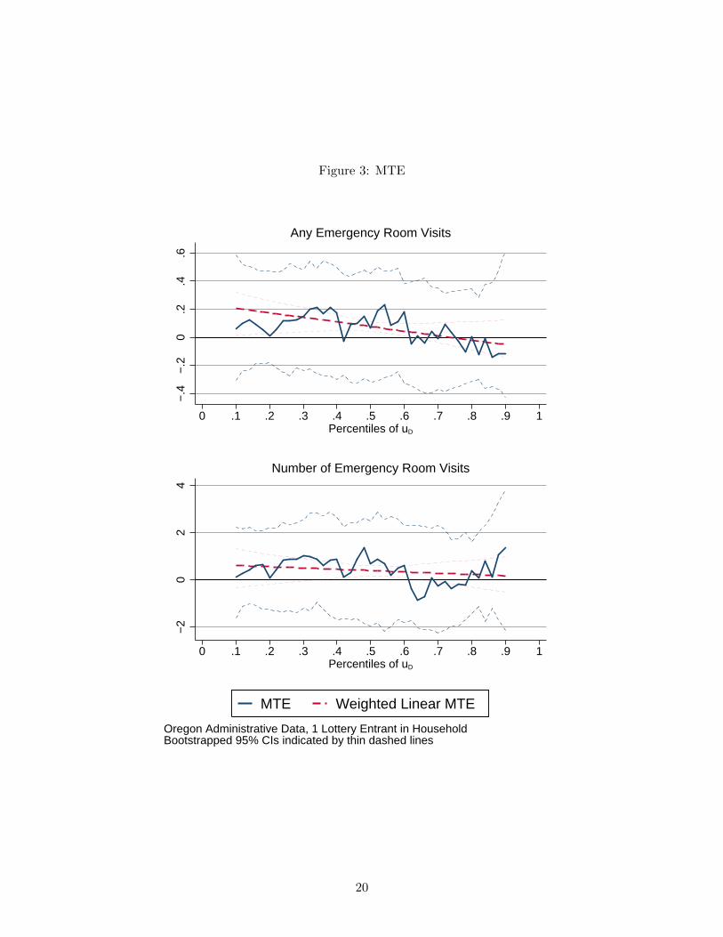
Figure 3: MTE−

.4−

.20

.2.4

.6

.1 .2 .3 .4 .5 .6 .7 .8 .90 1Percentiles of uD

Any Emergency Room Visits

−2

02

4

.1 .2 .3 .4 .5 .6 .7 .8 .90 1Percentiles of uD

Number of Emergency Room Visits

Oregon Administrative Data, 1 Lottery Entrant in HouseholdBootstrapped 95% CIs indicated by thin dashed lines

MTE Weighted Linear MTE

20

of taking up health insurance coverage based on observable characteristics increases, and hence as

the unobserved cost of taking up health insurance increases because the individuals at the margin

have not yet taken it up, the marginal treatment effect of health insurance on emergency room

utilization decreases. The line for the “any visit” outcome even crosses zero, and the line for the

“number of visits” outcome appears that it will cross zero slightly above the range of reported

values. Thus for some individuals within the OHIE, the MTE is positive, but for others, the MTE

is negative, depending on their observed probability of selecting into health insurance.

The estimated heterogeneity in the MTE function will lead to estimates of the local average

treatment effect (LATE) that differ from the average treatment effect (ATE), the average treatment

effect on the treated (ATT), and the average treatment effect on the untreated (ATUT). We can

obtain each of these quantities by applying the corresponding weights depicted in Figure 2 to the

MTE function. We present the results in Table 3.

The first row of Table 3 presents the LATE point estimates obtained by weighting the MTE

function. As they should be, these point estimates are very similar to the point estimates obtained

via the main IV regressions reported in Column (7) of Table 1 (an increase in the probability of

any visit of 5.5 percent as compared to 4.5 percent and an increase in the number of visits of

0.305 as compared to 0.227 visits). The LATE estimates obtained via weighting the MTE function

are not exactly the same as the LATE estimates obtained via the IV approach because the MTE

approach requires differentiation and subsequent integration, inducing error. The standard errors

bootstrapped by household ID reflect the larger estimation error (0.024 as compared to 0.022 for the

“any visit” outcome and 0.134 as compared to 0.129 for the “number of visits” outcome), although

the estimates are still statistically different from zero.

The point-wise 95% confidence intervals reported on the MTE function and the weighted linear

MTE reported in Figure 3 are wide at each point, never rejecting zero. However, aggregating the

MTE function into the LATE does reject zero. We are also able to reject zero for other treatment

effects.

The next row of Table 3 reports the estimate of the average treatment effect (ATE), obtained

by applying the ATE weights reported in Figure to the MTE functions reported in Figure 3. The

average treatment effect is larger than the local average treatment effect, indicating that if we had

a policy that signed all individuals up for coverage rather than allowing them to decide whether to

21

Table 3: Treatment Effects

sign up or not, then emergency room utilization would increase by even more than it did for the

compliers in the OHIE.

The next two rows of Table 3 report estimates of the average treatment effect on the untreated

(ATUT) and the average treatment effect on the treated (ATT), obtained by applying the respective

weights from Figure 2 to the MTE estimates in Figure 3. The ATT estimate places more weight

on the MTE estimates at the lower propensity scores where the MTE function is the largest.

Unsurprisingly, the ATT estimate is the largest estimate in the first column, indicating that among

individuals that would select into health insurance based on their observed characteristics and

unobserved costs of obtaining health insurance, health insurance increases the probability of an

emergency room visit by 9.4 percentage points. As expected given the weights and the shape of

the estimated MTE function, the average treatment effect on the untreated is much smaller than

the average treatment effect on the treated. The ATUT estimate indicates that among individuals

that entered the Oregon lottery who would not choose to select into health insurance based on their

observed characteristics and their unobserved costs of obtaining health insurance, health insurance

increases the probability of an emergency room visit by 2.6 percentage points.

22

6 Reconciling Effects from Oregon with Effects from Massachusetts

We have shown that the marginal treatment effect of health insurance on emergency room utilization

was positive for some types of individuals and negative for others in the OHIE. Thus, the external

validity of the OHIE depends on the types of individuals in the external applications of interest.

Here, we focus on the Massachusetts health reform as the external application of interest, and we

attempt to reconcile the decrease in emergency room visits observed in Massachusetts with the

results from the OHIE using MTE methods.

Before undertaking this exercise, we acknowledge that there are several factors that could have

differed between both empirical contexts that MTE methods will not address directly. At a fun-

damental level, the Oregon expansion was an RCT and the Massachusetts reform was a state-wide

policy. Therefore, the Oregon study is more likely to produce partial equilibrium impacts that are

internally consistent, and the Massachusetts health reform is more likely to produce general equilib-

rium impacts that have issues with internal consistency. Furthermore, institutional features of the

health care environment could differ across states. As discussed by Miller [2012], Massachusetts had

an uncompensated care pool that might have encouraged excess emergency care before its dissolu-

tion and replacement under the Massachusetts health reform. Also, both states could have different

social norms regarding emergency room vs. primary care usage. Health insurance terms could also

differ, especially since Oregon expanded Medicaid alone and Massachusetts also expanded other

types of coverage. MTE methods will hinge on differences in observable individual-level demo-

graphic characteristics; other differences will manifest themselves as differences in unobservables.

Table 4 presents observable demographic characteristics from the OHIE and Massachusetts side-

by-side. The data from the Massachusetts health reform are the same data from the Behavioral Risk

Factor Surveillance System (BRFSS) used by Kolstad and Kowalski [2012], restricted to include only

individuals from Massachusetts. As shown in the top row, these data do not include any measures

of emergency room utilization, but they do allow us to compare individual-level characteristics

from the Massachusetts health reform with individual-level characteristics from the OHIE. The

data from the other published studies that examine the impact of the Massachusetts health reform

on emergency room visits are not at the individual level, or they only include individuals who visit

the emergency room, making them unsuitable for this exercise.

23

Table 4: Summary Statistics

Oregon  Health  Insurance  Experiment

Oregon(Compliers)  

Massachusetts  Health  Reform  

Massachusetts(Compliers)

(1) (2) (3) (4)Y  (Any  ER  visit) 0.37 0.38 -­‐ -­‐Y  (Number  of  ER  visits,  censored) 1.12 1.20 -­‐ -­‐Z  (Selected  in  Oregon  lottery) 0.34 0.34 0.00 0.00Z  (Massachusetts,  Post-­‐Reform) 0.00 0.00 0.42 0.42D  (Any  insurance) 0.40 0.34 0.92 0.42D  (Medicaid) 0.24 0.34 -­‐ -­‐Lottery  entrants  in  household 1.00 1.00 -­‐ -­‐Number  of  adults  in  household -­‐ -­‐ 1.86 1.86Age  in  2009 40.7 42.6 42.0 42.5Female 0.56 0.53 0.51 0.43English 0.91 0.92 0.96 0.86

Number  of  Observations 19,643 6,200 62,541Oregon  summary  statistics  are  calculated  using  the  sample  of  observations  with  1  lottery  entrant  in  household.  English  is  defined  as  an  individual  choosing  materials  that  are  written  in  English.  Massachusetts  summary  statistics  are  derived  from  the  MA  sample  in  the  Behavioral  Risk  Factor  Surveillance  System  2004-­‐2009.  Note  that  for  this  sample,  there  are  more  people  in  the  treatment  group  than  in  the  control  group  because  we  have  more  years  of  data  in  the  post-­‐reform  period  than  in  the  pre-­‐reform  period.  The  pre-­‐reform  period  spans  2004  through  March  2006.  The  post-­‐reform  period  spans  July  2007  through  2009.  The  during-­‐reform  period,  which  spans  April  2006  through  June  2007,  has  been  excluded  from  the  analysis.

Summary  Statistics

To examine the Massachusetts health reform, we can define an alternative instrument Z that

indicates whether the individual was in the sample post-reform. As discussed in the table notes,

the Massachusetts sample includes slightly less data in the post-reform period (42%). Overall, the

Massachusetts sample from the BRFFSS includes 62,541 individuals, making it much larger than

our primary OHIE sample of 19,643 individuals.

In the full Massachusetts sample with the individuals from before and after the reform pooled,

rates of any health insurance coverage are 92% over the entire period, which is much higher the 40%

rate of coverage in the OHIE sample, which includes those who won and lost the lottery, suggesting

that the two samples likely consisted of very different people. The BRFSS data do not include a

variable that indicates whether health insurance coverage was through Medicaid.

24

As above, we restrict the OHIE sample to include only individuals in household with exactly

one lottery entrant. Unfortunately, the OHIE administrative data do not include information on

household size - we only know the number of lottery entrants. In the Massachusetts data, the

average individual is from a household with 1.86 individuals.

The next three rows compare the “common controls” available in the Oregon data and the Mas-

sachusetts data. As shown, the Oregon individuals are younger, they are more likely to be female,

and they are less likely to speak English. The subsequent column repeats the statistics reported in

Column (9) of Table 1, and the final column reports similar statistics for the Massachusetts sample.

From this exercise, we see that compliers in Oregon are even younger, more female, and less likely

to speak English than compliers in Massachusetts.

To further investigate the compliers in Massachusetts, we estimate propensity scores for the

probability of obtaining health insurance coverage using the same logit model from Oregon with

the Massachusetts data and with the instrument Z defined as post-reform. We plot the histogram

of the propensity scores in Massachusetts in Figure 4.

Figure 4: Distribution of Propensity Scores in Massachusetts

25

When we compare this figure to the analogous Figure 1 from Oregon, we notice several differ-

ences. One difference is that always takers comprise the bulk of the sample in Massachusetts at each

propensity score, even though they had a much more limited prevalence in Oregon. This makes

sense because the sample of people who signed up for a health insurance lottery in Oregon included

relatively few individuals who would obtain health insurance coverage regardless of whether they

won the lottery. In contrast, the vast majority of Massachusetts residents had coverage before the

reform, and the reform did not change their coverage. In fact, it is very difficult to see the counts

of control compliers or treatment compliers in Massachusetts because there are so many always

takers.

Figure 5 includes only the compliers so that it is easier to discern their distribution. It also

reports fractions of observations in each bin as opposed to counts of observations in each bin, where

the fractions have been calculated so that the treatment (after reform) and control (before reform)

groups have equal mass. This rescaling allows us to better visualize how the instrument (the reform)

shifted the probability of insurance to the right, bound by the upper limit of full insurance. Large

visual differences in the observed distributions of control compliers and treatment compliers would

raise concerns about the validity of the Massachusetts health reform as a quasi-experiment.

Another striking difference between Figure 1 and Figures 4 and 5 is that there is much more

mass to the right of the histogram in Massachusetts than there is in Oregon, which reflects the

higher average probability of having health insurance coverage. There was almost no mass above a

propensity score of 0.7 in Oregon, but almost all of the mass occurs above a propensity score of 0.7

in Massachusetts. If we interpret the propensity scores to be the observed benefit of treatment, then

the observed benefit of treatment is much higher than it is in Oregon. Therefore, individuals who are

at the margin of purchasing health insurance in Massachusetts must have much higher unobserved

costs of purchasing health insurance in Massachusetts relative to Oregon. This interpretation

of the distribution of propensity scores makes intuitive sense because individuals in the OHIE

sample who were uninsured signed up for a lottery for health insurance coverage, but individuals

in the Massachusetts sample who were uninsured were encouraged to purchase coverage through

the subsidies and mandates established by the Massachusetts health reform.2

2Putting this differently, there could have been more “selection on moral hazard” in the spirit of Einav et al.[2013] in Oregon than there was in Massachusetts. Indeed, Finkelstein et al. [2012] finds evidence of “selection onmoral hazard” within the OHIE in the sense that individuals who signed up for the lottery on the first day had larger

26

Figure 5: Distribution of Propensity Scores in Massachusetts, Only Compliers

0.0

5.1

.15

0 .1 .2 .3 .4 .5 .6 .7 .8 .9 1Propensity Score

Control CompliersTreatment Compliers

Behavioral Risk Factor Surveillance System 2004−2009, Massachusetts Data

Having established that the Oregon compliers had different observable characteristics than the

Massachusetts compliers and thus different propensity scores, we can use those differences in observ-

able characteristics to predict what should have happened to emergency room utilization following

the Massachusetts health reform using the LATE weights calculated from the Massachusetts data

applied to the MTE function estimated using the Oregon data.

Figure 6 reports the empirical weights estimated in the Massachusetts data. As discussed

regarding the analogous Figure 2 from Oregon, the LATE weights seem to have a strong relationship

with the propensity scores of the compliers. Just as most of the compliers have very high propensity

scores, the LATE weights put the most weight on very high propensity scores.

In fact, the LATE weights are almost entirely above the support of the Oregon data, so we cannot

directly apply the Massachusetts weights to the Oregon MTE without extrapolating the Oregon

MTE to the right. As discussed above, the red dashed lines in Figure 3 give the linear extrapolation,

which shows that the treatment effect of health insurance on emergency room utilization is negative

to the right of the Oregon support. Miller [2012] finds that individuals who gained health insurance

takeup and utilization point estimates than individuals who signed up later.

27

Figure 6: MTE Weights Massachusetts

coverage through the Massachusetts health reform had 0.5 fewer emergency room visits per year.

Some reasonable extrapolation from the MTE could yield a negative point estimate of a similar

magnitude. However, the results that we obtain for the Massachusetts LATE in this way are very

sensitive to the type of extrapolation that we perform. Rather than reporting a point estimate, we

simply conclude that the Oregon MTE function implies that the LATE impact of the Massachusetts

health reform on emergency room utilization was negative, as shown by the literature. We have

thus reconciled results from Oregon and results from Massachusetts using MTE methods.

7 Treatment Effect Heterogeneity

The key to our reconciliation of the Oregon and Massachusetts results is the finding that the

marginal treatment effect of health insurance on emergency room utilization was positive for some

types of individuals and negative for others in the OHIE. In this section, we consider whether the

standard method to examine treatment effect heterogeneity would have yielded a similar finding.

The standard method to examine treatment effect heterogeneity is to break the estimation sample

28

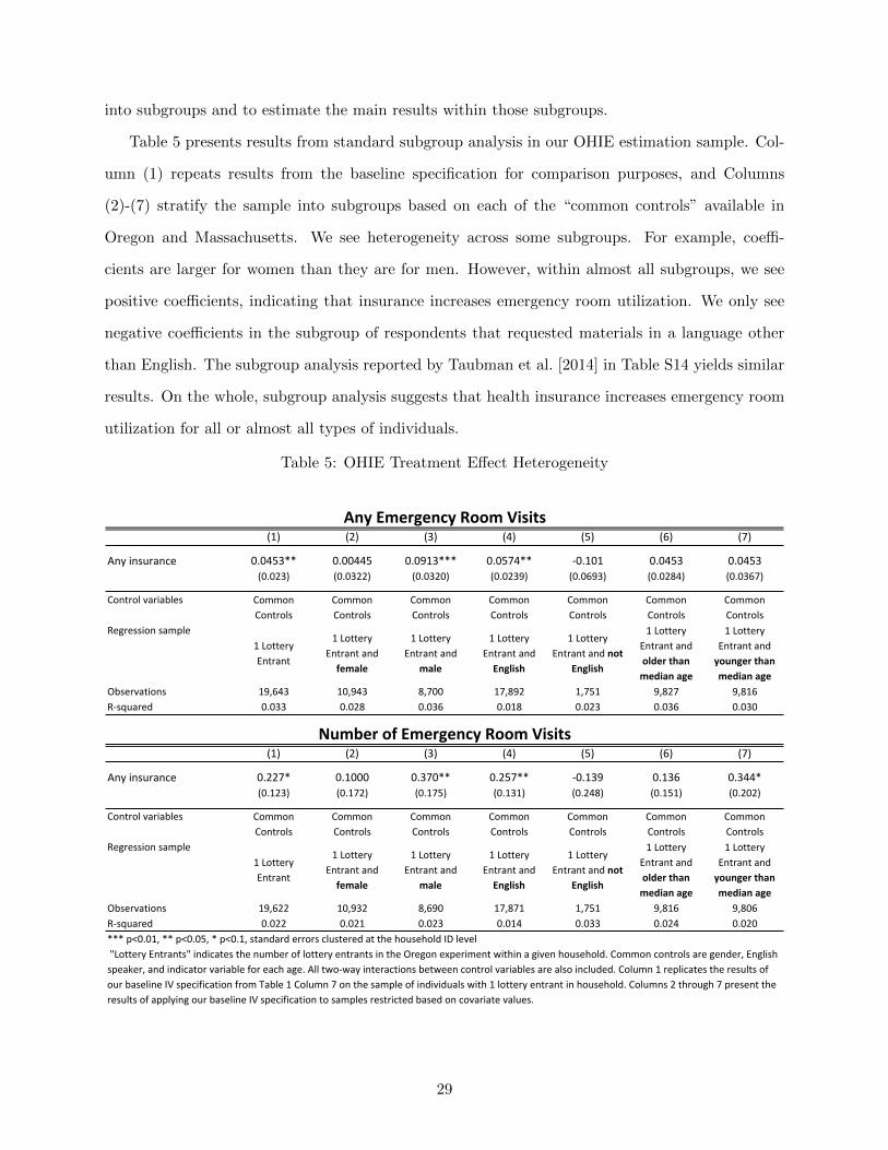
into subgroups and to estimate the main results within those subgroups.

Table 5 presents results from standard subgroup analysis in our OHIE estimation sample. Col-

umn (1) repeats results from the baseline specification for comparison purposes, and Columns

(2)-(7) stratify the sample into subgroups based on each of the “common controls” available in

Oregon and Massachusetts. We see heterogeneity across some subgroups. For example, coeffi-

cients are larger for women than they are for men. However, within almost all subgroups, we see

positive coefficients, indicating that insurance increases emergency room utilization. We only see

negative coefficients in the subgroup of respondents that requested materials in a language other

than English. The subgroup analysis reported by Taubman et al. [2014] in Table S14 yields similar

results. On the whole, subgroup analysis suggests that health insurance increases emergency room

utilization for all or almost all types of individuals.

Table 5: OHIE Treatment Effect Heterogeneity

Any  Emergency  Room  Visits(1) (2) (3) (4) (5) (6) (7)

Any  insurance 0.0453** 0.00445 0.0913*** 0.0574** -­‐0.101 0.0453 0.0453(0.023) (0.0322) (0.0320) (0.0239) (0.0693) (0.0284) (0.0367)

Control  variables Common  Controls

Common  Controls

Common  Controls

Common  Controls

Common  Controls

Common  Controls

Common  Controls

Regression  sample1  Lottery  Entrant

1  Lottery  Entrant  and  female

1  Lottery  Entrant  and  

male

1  Lottery  Entrant  and  English

1  Lottery  Entrant  and  not  

English

1  Lottery  Entrant  and  older  than  median  age

1  Lottery  Entrant  and  younger  than  median  age

Observations 19,643 10,943 8,700 17,892 1,751 9,827 9,816R-­‐squared 0.033 0.028 0.036 0.018 0.023 0.036 0.030

Number  of  Emergency  Room  Visits(1) (2) (3) (4) (5) (6) (7)

Any  insurance 0.227* 0.1000 0.370** 0.257** -­‐0.139 0.136 0.344*(0.123) (0.172) (0.175) (0.131) (0.248) (0.151) (0.202)

Control  variables Common  Controls

Common  Controls

Common  Controls

Common  Controls

Common  Controls

Common  Controls

Common  Controls

Regression  sample1  Lottery  Entrant

1  Lottery  Entrant  and  female

1  Lottery  Entrant  and  

male

1  Lottery  Entrant  and  English

1  Lottery  Entrant  and  not  

English

1  Lottery  Entrant  and  older  than  median  age

1  Lottery  Entrant  and  younger  than  median  age

Observations 19,622 10,932 8,690 17,871 1,751 9,816 9,806R-­‐squared 0.022 0.021 0.023 0.014 0.033 0.024 0.020***  p<0.01,  **  p<0.05,  *  p<0.1,  standard  errors  clustered  at  the  household  ID  level  "Lottery  Entrants"  indicates  the  number  of  lottery  entrants  in  the  Oregon  experiment  within  a  given  household.  Common  controls  are  gender,  English  speaker,  and  indicator  variable  for  each  age.  All  two-­‐way  interactions  between  control  variables  are  also  included.  Column  1  replicates  the  results  of  our  baseline  IV  specification  from  Table  1  Column  7  on  the  sample  of  individuals  with  1  lottery  entrant  in  household.  Columns  2  through  7  present  the  results  of  applying  our  baseline  IV  specification  to  samples  restricted  based  on  covariate  values.

29

0.1

.2.3

.4.5

−6.0 −4.0 −2.0 0.0 2.0

Any Emergency Room Visits−IV coefficients

(a) Any Emergency Room Visits

0.0

5.1

.15

.2

−20.0 −10.0 0.0 10.0 20.0

Number of Emergency Room Visits−IV coefficients

(b) Number of Emergency Room Visits

Figure 7: Distributions of IV Coefficients

However, it is possible that standard subgroup analysis along observable dimensions obscures

treatment effect heterogeneity along unobservable dimensions. For example, although the coefficient

estimated among women only is positive, there could be some women with positive treatment effects

and other women with negative treatment effects. To further investigate this claim, we divide the

sample into smaller subgroups based on all three “common controls.” We identify all distinct cells

based on all combinations of gender, English speaking status, and age in years, resulting in 176

distinct subgroups, and we re-run our baseline regression within each subgroup.3 In Figure 7, we

present histograms that report the distribution of estimated IV coefficients across all subgroups,

with the “any visits” outcome on the left and the “number of visits” outcome on the right. This

finer subgroup analysis tells a different story - it appears that just under half of subgroups yield

negative coefficients.

A natural follow-up question involves asking who is in the subgroups with negative IV coeffi-

cients. We present summary statistics on these individuals in Table 6. Column (3) shows that in

our finer subgroup analysis, around 40% of individuals have negative IV coefficients for the “any

visit” outcome, and Column (4) shows that a slightly higher fraction of individuals have negative IV

coefficients for the “number of visits” outcome. Comparing the characteristics of these individuals

with the characteristics of individuals in the full sample, reported in Column (1), we see that indi-

viduals in subgroups with negative IV coefficients are older, more likely to be female, and less likely

3The cell sizes in some subgroups are very small. We re-ran our analysis using only subgroups with 100 or moreobservations, and the results were similar.

30

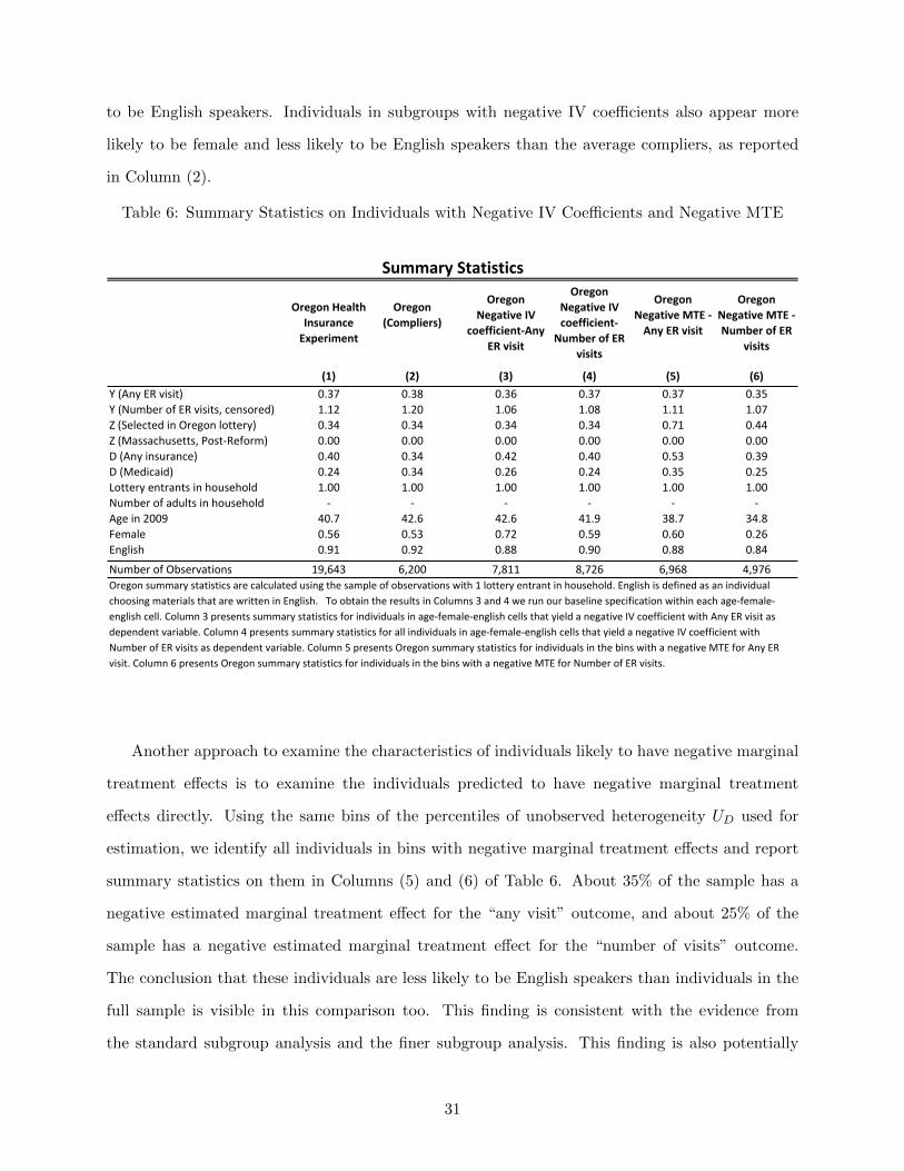
to be English speakers. Individuals in subgroups with negative IV coefficients also appear more

likely to be female and less likely to be English speakers than the average compliers, as reported

in Column (2).

Table 6: Summary Statistics on Individuals with Negative IV Coefficients and Negative MTE

Oregon  Health  Insurance  Experiment

Oregon(Compliers)  

Oregon  Negative  IV  

coefficient-­‐Any  ER  visit

Oregon  Negative  IV  coefficient-­‐

Number  of  ER  visits

Oregon  Negative  MTE  -­‐  Any  ER  visit  

Oregon  Negative  MTE  -­‐  Number  of  ER  

visits  

(1) (2) (3) (4) (5) (6)Y  (Any  ER  visit) 0.37 0.38 0.36 0.37 0.37 0.35Y  (Number  of  ER  visits,  censored) 1.12 1.20 1.06 1.08 1.11 1.07Z  (Selected  in  Oregon  lottery) 0.34 0.34 0.34 0.34 0.71 0.44Z  (Massachusetts,  Post-­‐Reform) 0.00 0.00 0.00 0.00 0.00 0.00D  (Any  insurance) 0.40 0.34 0.42 0.40 0.53 0.39D  (Medicaid) 0.24 0.34 0.26 0.24 0.35 0.25Lottery  entrants  in  household 1.00 1.00 1.00 1.00 1.00 1.00Number  of  adults  in  household -­‐ -­‐ -­‐ -­‐ -­‐ -­‐Age  in  2009 40.7 42.6 42.6 41.9 38.7 34.8Female 0.56 0.53 0.72 0.59 0.60 0.26English 0.91 0.92 0.88 0.90 0.88 0.84

Number  of  Observations 19,643 6,200 7,811 8,726 6,968 4,976

Summary  Statistics

Oregon  summary  statistics  are  calculated  using  the  sample  of  observations  with  1  lottery  entrant  in  household.  English  is  defined  as  an  individual  choosing  materials  that  are  written  in  English.      To  obtain  the  results  in  Columns  3  and  4  we  run  our  baseline  specification  within  each  age-­‐female-­‐english  cell.  Column  3  presents  summary  statistics  for  individuals  in  age-­‐female-­‐english  cells  that  yield  a  negative  IV  coefficient  with  Any  ER  visit  as  dependent  variable.  Column  4  presents  summary  statistics  for  all  individuals  in  age-­‐female-­‐english  cells  that  yield  a  negative  IV  coefficient  with  Number  of  ER  visits  as  dependent  variable.  Column  5  presents  Oregon  summary  statistics  for  individuals  in  the  bins  with  a  negative  MTE  for  Any  ER  visit.  Column  6  presents  Oregon  summary  statistics  for  individuals  in  the  bins  with  a  negative  MTE  for  Number  of  ER  visits.

Another approach to examine the characteristics of individuals likely to have negative marginal

treatment effects is to examine the individuals predicted to have negative marginal treatment

effects directly. Using the same bins of the percentiles of unobserved heterogeneity UD used for

estimation, we identify all individuals in bins with negative marginal treatment effects and report

summary statistics on them in Columns (5) and (6) of Table 6. About 35% of the sample has a

negative estimated marginal treatment effect for the “any visit” outcome, and about 25% of the

sample has a negative estimated marginal treatment effect for the “number of visits” outcome.

The conclusion that these individuals are less likely to be English speakers than individuals in the

full sample is visible in this comparison too. This finding is consistent with the evidence from

the standard subgroup analysis and the finer subgroup analysis. This finding is also potentially

31

consistent with the subgroup analysis from Taubman et al. [2014], which does not divide the sample

along this dimension. Perhaps individuals who do not speak English are less likely to increase their

emergency room utilization when they gain access to health insurance.

Our analysis has shown that MTE methods can illuminate treatment effect heterogeneity that

can go undetected with standard subgroup analysis. However, the treatment effect heterogeneity

that the MTE identifies along the unobservable dimensions does appear to have a basis along the

observable dimension. Finer subgroup analysis suggests that individuals with negative marginal

treatment effects have similar observable characteristics to individuals with negative IV coefficients

in the sense that they are less likely to be English speakers.

One limitation of subgroup analysis is that it requires large treatment effects or really large

samples to detect treatment effect heterogeneity. MTE methods can also be underpowered at

detecting treatment effect heterogeneity. However, by maintaining assumptions that incorporate

evidence from subgroups with similar propensities of taking up treatment, they require less power.

In future work, I would like to attempt to increase the power of MTE methods by using machine

learning methods to select the included covariates.

8 Robustness

In all of the reported results, we have focused on the sample of households with a single lottery

entrant on the grounds that households similar to those will be easier to identify in other contexts.

To examine robustness, we repeat the analysis on the sample of households with two or more

entrants and on the pooled sample that includes all households regardless of the number of entrants

and an additional covariate separating households with one entrant from other households. We

report the results in Appendix D.

We first consider the sample of households with two or more lottery entrants. As shown through

the comparison of Figure D1 to Figure 1, participants in this sample have higher propensities of

obtaining health insurance than participants with a single lottery entrant, as predicted based on

the same set of demographic characteristics. Furthermore, as shown in Figure D2, the participants

with high propensities of obtaining health insurance among this sample get the highest weights in

the LATE estimate.

32

Figure D3 reports the estimated MTE function on the sample of participants with two or more

lottery entrants in their household. The vertical axis in this figure covers a much wider range

than the vertical axis is the corresponding Figure 3 for participants with a single household lottery

entrant, and most of the marginal treatment effects are more positive. Furthermore, the line fit

to the MTE, depicted in red, is upward sloping. Given that the LATE on this sample places the

most weight toward the right of the support, it is not surprising that the LATE estimated on

this sample is much larger than the LATE obtained in the sample with a single lottery entrant, as

previously shown in Columns (5) and (6) of Table 1. Table D1 shows the treatment effects obtained

by weighting the MTE function and shows similarly large LATE estimates for both estimates of

the dependent variable, estimated less precisely.

When we pool the sample of households with two or more lottery entrants with the primary

estimation sample with a single lottery entrant, we see more mass in higher propensity scores of

Figure D1, and the LATE weights in Figure D5 continue to place weight in the same ranges as the

sample that includes a single lottery entrant. The MTE function in this pooled sample, reported

in Figure D6 shows substantial heterogeneity. It is negative in some ranges and positive in others,

and it increases toward the right of the range. However, the line fit to the MTE and the LATE

reported in Table D2 mask this heterogeneity, showing only a positive impact of health insurance

on emergency room utilization.

Given the patterns in the MTE that we observed in the sample of 2 ore more lottery entrants

on its own and the distribution of propensity scores in that sample, it seems likely that participants

in that sample are responsible for the upward slope in the MTE function toward the higher values

of the percentiles of UD. If we extrapolated from Oregon to Massachusetts using the MTE function

from the pooled sample, we would be likely to conclude that emergency room utilization would

increase even more in Massachusetts than it did in Oregon. However, such extrapolation might not

be reasonable because marginal individuals who gain health insurance in Massachusetts are unlikely

to be similar to individuals in Oregon who had more than one lottery entrant in their household.

Therefore, we prefer extrapolation based on our main sample.

33

9 Experimental Design for External Validity

The exercise of applying MTE methods to the OHIE has brought to light several issues that could

be considered in the design of future experiments to maximize the usefulness of MTE methods in

examining external validity. The first issue is that a wide array of covariates should be collected

to aid in tracing out a nonlinear MTE function. Ideally, these covariates should be defined such

that they can also be obtained from other experimental or non-experimental data. By defining

covariates in a standardized fashion, the MTE function from one context such as Oregon can be

applied to another such as Massachusetts.

A second issue is that covariates used for stratification should be defined such that they can

also be obtained from other experimental or non-experimental data. In the case of the OHIE,

recall that multiple members of the same household could sign up for the health insurance lottery

independently. However, if any member of the household won the lottery, then all members of the

household were treated as winners. Thus, individuals in households with multiple entrants had a

higher probability of winning. As shown in Table 1, the main results show that emergency room

utilization increased in response to increased insurance in Column (1) depend on a control for the

number of lottery entrants. If that control is removed as in Column (4), then the effect reverses

sign, and it loses its statistical significance. To be clear, stratifying on the number of lottery

entrants creates no problems for internal validity, but external validity is harder to assess because

it is unlikely that other data sets will contain information on how many household members would

enter a lottery were one to be offered.

A third issue is that there must be data on always takers, never takers, and compliers to

estimate the MTE function via the separate estimation approach. If researchers do not collect

follow-up data on experimental subjects who lose the lottery but attain the intervention by other

means, then always takers cannot be identified. Because the OHIE researchers collected data on

such individuals who lost the lottery but gained health insurance through other means, the MTE

function can be estimated. However, if they did not collect such data, as is common in clinical

trials, then only one of the separate pieces of the MTE function could be estimated.

A subtler issue is that the experiment or quasi-experiment must be designed such that always

takers and never takers are possible. If there is no way to attain the intervention outside the

34

lottery (no “always takers”) or if all participants who win the lottery take up the intervention (no

“never takers”), then the full MTE function cannot be estimated. For example, in their empirical

application, Brinch et al. [2012] cannot estimate the full MTE because there are no never takers

who have twins but do not end up with an extra child.

A related issue is that going to great lengths to encourage all participants who win the lottery

to receive the intervention, and conversely to discourage all participants who lost the lottery to

forgo intervention, could decrease the external validity of the estimates obtained. It could also

limit the ability of the researchers to use the estimates to produce externally relevant ones. In the

extreme case, if there is no selection into or out of treatment, then the MTE cannot be estimated.

In that case, the local average treatment effect (LATE) will be equal to the average treatment effect

(ATE). However, if the policy intervention based on the experiment will allow individuals to select

into or out of treatment, then the researchers might prefer an alternative LATE to the ATE for

purposes of external validity. For example, as shown in Table 3, in the OHIE application, the ATE

is larger than the LATE, meaning that if the policy intervention required everyone to select into

health insurance, then emergency room visits would increase by even more than they did under the

OHIE. Realistic policy interventions would probably be more likely to offer health insurance for

free or to require individuals to pay a penalty if they choose not to select into health into health

insurance, so the ATE might not be the parameter of interest.

Another manifestation of going to great lengths to encourage full takeup of the experimental

lottery is that the estimated ATE could be smaller than the LATE that would result from an

externally relevant policy. In the OHIE context, we find that the ATE is larger than the LATE.

However, the ATE could be smaller than the LATE in other contexts. For example, suppose that

the individuals with the largest benefits from a new medical intervention select into treatment

first after winning the lottery. Encouraging others to select into treatment will reduce the LATE,

bringing it closer to the ATE, and making the intervention appear less effective. In this way,

companies that hope to show a benefit of a new medical intervention could attain smaller estimates

if they are more diligent about encouraging full takeup. Furthermore, unless the relevant policy

intervention would involve full takeup, these smaller estimates will not be externally valid.

35

10 Conclusion

I examine the external validity of the Oregon Health Insurance Experiment (OHIE) using marginal

treatment effect (MTE) methods. A central finding from the OHIE is that individuals who gained

health insurance through the OHIE lottery increased their emergency room utilization (Taubman

et al. [2014]). Using data from the OHIE, I find that that the marginal treatment effect of health

insurance on emergency room utilization was positive for some types of individuals and negative for

others. Thus, the external validity of the finding that emergency room utilization increases when

health insurance expands depends on the types of individuals who gain coverage.

Using data from Kolstad and Kowalski [2012], I reexamine the types of individuals who gained

coverage through the Massachusetts health reform, which established a mandate for uninsured

individuals to purchase coverage or pay a penalty, among other interventions. I find that the

Massachusetts individuals induced to gain health insurance appear more similar to the Oregon

individuals that decreased their emergency room utilization than they do to the Oregon individuals

that increased their emergency room utilization. Furthermore, on the whole, individuals who

entered a lottery for health insurance coverage in Oregon likely had a higher desire to use the

emergency room than individuals who gained coverage when a mandated required them to do so in

Massachusetts. Therefore, it is not surprising that that literature finds decreases in emergency room

utilization in Massachusetts despite increases in Oregon because the two state policy interventions

expanded coverage to different types of individuals.

Given that my findings deepen our understanding of the external validity of the OHIE, I con-

clude that MTE methods will be a valuable addition to the standard toolkit for analysis of ex-

periments and quasi-experiments with binary treatments. However, marginal treatment effects do

not supplant existing methods to used to examine external validity. There are several factors that

could have differed between both empirical contexts, including those explicitly taken into account

by MTE methods, such as the demographic characteristics of participants, and those that are not

explicitly taken into account by MTE methods, such as institutional features of emergency rooms.

Based on my analysis, I highlight several research design considerations that can maximize the

ability of MTE methods to shed light on external validity in future applications.

36

References

Michael Anderson, Carlos Dobkin, and Tal Gross. The effect of health insurance coverage on the

use of medical services. American Economic Journal: Economic Policy, 4(1):1–27, 2012. doi:

10.1257/pol.4.1.1. URL http://www.aeaweb.org/articles.php?doi=10.1257/pol.4.1.1.

Michael L Anderson, Carlos Dobkin, and Tal Gross. The effect of health insurance on emergency

department visits: Evidence from an age-based eligibility threshold. Review of Economics and

Statistics, 96(1):189–195, 2014.

Joshua D. Angrist and Jorn-Steffen Pischke. Mostly Harmless Econometrics: An Empiricists’

Companion. Princeton University Press, 2009.

Anders Bjorklund and Robert Moffitt. The estimation of wage gains and welfare gains in self-

selection models. The Review of Economics and Statistics, pages 42–49, 1987.

BRFSS. Behavioral risk factor surveillance system survey data. Center for Disease Control. URL

http://www.cdc.gov/brfss/annual_data/annual_2013.html.

Christian N Brinch, Magne Mogstad, and Matthew James Wiswall. Beyond late with a discrete

instrument. heterogeneity in the quantity-quality interaction of children. Technical report, Re-

search Department of Statistics Norway, 2012.

Christopher Chen, Gabriel Scheffler, and Amitabh Chandra. Massachusetts’ health care reform

and emergency department utilization. New England Journal of Medicine, 365(12):e25, 2011.

Janet Currie and Jonathan Gruber. Health insurance eligibility and child health: lessons from

recent expansions of the medicaid program. Quarterly Journal of Economics, 111(2):431–466,

1996.

OHIE data. Oregon health insurance experiment public use data. Finkelstein, Amy. URL http:

//www.nber.org/oregon/data.html.

Liran Einav, Amy Finkelstein, Stephen Ryan, Paul Schrimpf, and Mark R Cullen. Selection on

moral hazard in health insurance. The American Economic Review, 103(1):178, 2013.

37

Amy F. Finkelstein, Sarah Taubman, Bill J. Wright, Mira Bernstein, Jonathan Gruber, Joseph P.

Newhouse, Heidi L. Allen, Katherine Baicker, and the Oregon Health Study Group. The oregon

health insurance experiment: Evidence from the first year. The Quarterly Journal of Economics,

127(3):1057–1106, 2012. doi: 10.1093/qje/qjs020.

Amy F. Finkelstein, Nathaniel Hendren, and Erzo F.P. Luttmer. The value of medicaid interpreting

results from the oregon health insurance experiment. June 2015. URL http://economics.mit.

edu/files/10580.

Jerry A Hausman. Specification tests in econometrics. Econometrica: Journal of the Econometric

Society, pages 1251–1271, 1978.

James Heckman, Sergio Urzua, and Edward Vytlacil. Estimation of treatment effects under essential

heterogeneity. 2006. URL http://jenni.uchicago.edu/underiv/documentation_2006_03_

20.pdf.

James J. Heckman and Edward Vytlacil. Structural Equations, Treatment Effects, and Econometric

Policy Evaluation. Econometrica, 73(3):669–738, 05 2005. URL http://ideas.repec.org/a/

ecm/emetrp/v73y2005i3p669-738.html.

James J Heckman and Edward J Vytlacil. Local instrumental variables and latent variable models

for identifying and bounding treatment effects. Proceedings of the national Academy of Sciences,

96(8):4730–4734, 1999.

James J Heckman and Edward J Vytlacil. Econometric evaluation of social programs, part ii:

Using the marginal treatment effect to organize alternative econometric estimators to evaluate

social programs, and to forecast their effects in new environments. Handbook of econometrics, 6:

4875–5143, 2007.

Guido W. Imbens and Joshua D. Angrist. Identification and estimation of local average treatment

effects. Econometrica, 62(2):467–75, 1994.

Jonathan T. Kolstad and Amanda E. Kowalski. The impact of health care reform on hospital

and preventive care: Evidence from massachusetts. Journal of Public Economics, 96:909–929,

December 2012.

38

Sarah Miller. The effect of insurance on emergency room visits: an analysis of the 2006 mas-

sachusetts health reform. Journal of Public Economics, 96(11):893–908, 2012.

Joseph P. Newhouse and Rand Corporation Insurance Experiment Group. Free for all?: lessons

from the RAND health insurance experiment. Harvard University Press, 1993.

Peter B. Smulowitz, Robert Lipton, J. Frank Wharam, Leon Adelman, Scott G. Weiner, Laura

Burke, Christopher W. Baugh, Jeremiah D. Schuur, Shan W. Liu, Meghan E. McGrath, Bella Liu,

Assaad Sayah, Mary C. Burke, J. Hector Pope, and Bruce E. Landon. Emergency department uti-

lization after the implementation of massachusetts health reform. Annals of Emergency Medicine,

58(3):225 – 234.e1, 2011. ISSN 0196-0644. doi: http://dx.doi.org/10.1016/j.annemergmed.2011.

02.020. URL http://www.sciencedirect.com/science/article/pii/S0196064411001338.

Sarah L. Taubman, Heidi L. Allen, Bill J. Wright, Katherine Baicker, and Amy N. Finkel-

stein. Medicaid increases emergency-department use: Evidence from oregon’s health insur-

ance experiment. Science, 343(6168):263–268, 2014. doi: 10.1126/science.1246183. URL

http://www.sciencemag.org/content/343/6168/263.abstract.

Appendices

A Weights

LATE Weights

ωLATE(x, uD) =(E(J |P (W ) > uD, X = x)− E(J |X = x)) Pr(P (W ) > uD|X = x)

Cov(J,D|X = x)(4)

ATE Weights

ωATE(x, uD) = 1 (5)

ATT Weights

ωTT (x, uD) =Pr(P (W ) > uD|X = x)∫

Pr(P (W ) > uD|X = x)duD(6)

39

ATUT Weights

ωTUT (x, uD) =Pr(P (W ) ≤ uD|X = x)∫

Pr(P (W ) ≤ uD|X = x)duD(7)

B MTE Estimation Algorithm

Step 1

We estimate a logit model of treatment D on W , which consists of the instrument Z and the

covariates X. We do not interact Z with X, although X does include interaction terms. Using

the coefficient estimates, we predict a propensity score µD(W ) for each individual. In our context,

this propensity score represents the probability of having insurance for an individual with a given

vector of covariates X = x and a given value of the instrument Z = z.

Step 2

Next, we define the maximum interval of common support for the propensity score conditional on

D = 1, and the propensity score conditional on D = 0. We drop those observations outside of the

common support.

Step 3

We next transform our propensity score into a new propensity score P (W ) ≡ FUD(µD(W )) defined

as the quantiles of the estimated propensity score. This step represents a departure from Brinch

et al. [2012]. The advantage of our approach is that each point in the support of the new propen-

sity score has the same number of observations (approximately because we allow for ties between

observations with the same values x and z). Brinch et al. [2012] trim the sample of untransformed

propensity scores µD(W ) within the common support from Step 2 by a further 1% at both ends.

Instead, we trim our sample based on the transformed propensity scores P (W ), only reporting

estimates below above the 10th percentile and below the 90th percentile. We choose an estimation

grid P with associated bandwidth h within this range. Once it is chosen, we keep it fixed for all

subsequent steps, including each replication of the bootstrap routine.

40

Step 4

In Equation (3), we have expressed the MTE as

MTE(x, p) = E(Y1 − Y0|X = x, UD = p) = (β1 − β0)′x+ k(p).

In this step, we begin the “separate estimation approach:” we separately estimate β1 and β0

using double residual regression (we turn to estimating k(p) in Step 5). We perform double residual

regression one time to estimate β0 using the sample conditional on D = 0 and a second time to

estimate β1 using the sample conditional on D = 1. For each double residual regression, we first

run a local linear regression of Y on P (W ), using the grid P determined in Step 3. We save the

residual and call it eY , following Heckman et al. [2006]. We next run a local linear regression of

each value x on P (W ) and save the residual, calling it eX . Finally, we run a regression of eY on

all of the saved values of eX . The coefficients we estimate are β0 when the sample is restricted to

D = 0 and β1 when the sample is restricted to D = 1.

Step 5

Next, we turn to estimating the function k(p). As with β1 and β0, we must separately estimate

functions K1(p) and K0(p). To estimate K1(p) , we begin by defining Y1 as

Y1 = Y − β1X = K1(P (W )) + v.

We obtain coefficient estimates for K1(p) by running local linear regression of Y1 on the propensity

score P (W ) at each of the points in our grid P. We estimate K0 similarly, with Y0 instead defined

as

Y0 = Y − β0X = K0(P (W )) + v.

Step 6

The unobservable component of the MTE, k(p), is defined as

k(p) = k1(p)− k0(p),

41

which gives the difference between the unobservable component of Y1 given the treatment D = 1,

and the unobservable component of Y0 given the absence of treatment D = 0. k1(p) is the derivative

of K1(p) with respect to p, and k0(p) is the derivative of K0(p) with respect to p. Using the formulas

on page 7 of Brinch et al. [2012] and K1(p) and K0(p) obtained in Step 5, we calculate k1(p) and

k0(p). We take the difference between k1(p) and k0(p) to obtain k(p).

Step 7

With β1, β0, and k(p) estimated, we can finally calculate our MTE using Equation (3). Again, the

formula is

MTE(x, p) = (β1 − β0)′x+ k(p).

This gives us the MTE as a function of each set of characteristics x and each point p in our grid P.

To present the MTE as a function only of p, which we report in the figures, we take the weighted

average MTE over the characteristics x at each point p in our grid P.

C Average Marginal Effects from Logit Model

42

Table C1: Any Insurance Decision Model - Average Marginal Effects

Any  Insurance  Decision  Model  -­‐  Average  Marginal  EffectsAny  Insurance Any  Insurance

Z  (Selected  in  Oregon  lottery) 0.289***(0.00558)

Female 0.105***(0.00657)

English 0.0440***(0.0115)

Age  ≤21 -­‐ Age  =  43 -­‐0.0142-­‐ (0.0300)

Age  =  22 0.00474 Age  =  44 -­‐0.0315(0.0285) (0.0279)

Age  =  23 0.0105 Age  =  45 0.0485*(0.0276) (0.0287)

Age  =  24 -­‐0.0332 Age  =  46 0.0197(0.0280) (0.0289)

Age  =  25 -­‐0.0215 Age  =  47 -­‐0.036(0.0280) (0.0271)

Age  =  26 0.0252 Age  =  48 -­‐0.000693(0.0284) (0.0278)

Age  =  27 0.0334 Age  =  49 -­‐0.00974(0.0267) (0.0271)

Age  =  28 -­‐0.0237 Age  =  50 0.0103(0.0273) (0.0286)

Age  =  29 0.0421 Age  =  51 0.0305(0.0274) (0.0290)

Age  =  30 0.0175 Age  =  52 0.0393(0.0282) (0.0288)

Age  =  31 0.039 Age  =  53 0.0191(0.0287) (0.0280)

Age  =  32 0.0134 Age  =  54 0.0276(0.0279) (0.0276)

Age  =  33 0.0329 Age  =  55 0.0295(0.0297) (0.0298)

Age  =  34 -­‐0.0079 Age  =  56 0.0313(0.0290) (0.0297)

Age  =  35 0.0701** Age  =  57 0.0152(0.0298) (0.0295)

Age  =  36 0.00852 Age  =  58 0.0396(0.0299) (0.0317)

Age  =  37 0.0147 Age  =  59 0.0427(0.0298) (0.0321)

Age  =  38 -­‐0.00467 Age  =  60 0.0587*(0.0286) (0.0323)

Age  =  39 0.0190 Age  =  61 -­‐0.0112(0.0289) (0.0346)

Age  =  40 0.0059 Age  =  62 0.0472(0.0284) (0.0326)

Age  =  41 -­‐0.0188 Age  =  63 0.0351(0.0290) (0.0362)

Age  =  42 0.0277 Age  =  64 -­‐0.0376(0.0299) (0.0371)

Observations 19,643Mean  of  D  in  control  group 0.29 Mean  of  D  in  treatment  group 0.61

***  p<0.01,  **  p<0.05,  *  p<0.1Standard  errors,  clustered  at  the  household  ID  level,  in  parentheses.The  results  displayed  in  this  table  are  average  marginal  effects  computed  using  the  estimates  from  a  logit  model  in  which  we  included  all  of  these  variables  and  all  two-­‐way  interactions  between  the  control  variables  (i.e.  all  variables  displayed,  except  for  the  instrument  Z).

43

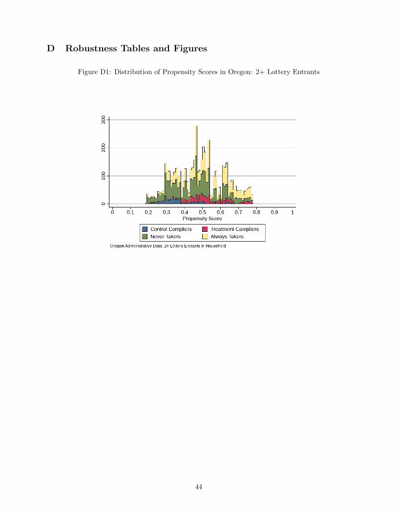
D Robustness Tables and Figures

Figure D1: Distribution of Propensity Scores in Oregon: 2+ Lottery Entrants

44

Figure D2: MTE Weights: 2+ Lottery Entrants

0.5

11.

52

2.5

0 .1 .2 .3 .4 .5 .6 .7 .8 .9 1Percentiles of UD

LATE ATTATUT ATE

Oregon Administrative Data, 2+ Lottery Entrants in Household

MTE Weights

Table D1: Treatment Effects: 2 + Lottery Entrants

45

Figure D3: MTE: 2+ Lottery Entrants−

1−

.50

.51

1.5

.1 .2 .3 .4 .5 .6 .7 .8 .90 1Percentiles of uD

Any Emergency Room Visits

−2

02

46

.1 .2 .3 .4 .5 .6 .7 .8 .90 1Percentiles of uD

Number of Emergency Room Visits

Oregon Administrative Data, 2 Lottery Entrants in HouseholdBootstrapped 95% CIs indicated by thin dashed lines

MTE Weighted Linear MTE

46

Figure D4: Distribution of Propensity Scores in Oregon: Pooled Lottery Entrants

Figure D5: MTE Weights: Pooled Lottery Entrants

0.5

11.

52

0 .1 .2 .3 .4 .5 .6 .7 .8 .9 1Percentiles of UD

LATE ATTATUT ATE

Oregon Administrative Data

MTE Weights

47

Figure D6: MTE: Pooled Lottery Entrants−

.50

.51

.1 .2 .3 .4 .5 .6 .7 .8 .90 1Percentiles of uD

Any Emergency Room Visits

−2

02

4

.1 .2 .3 .4 .5 .6 .7 .8 .90 1Percentiles of uD

Number of Emergency Room Visits

Oregon Administrative Data, Pooled SampleBootstrapped 95% CIs indicated by thin dashed lines

MTE Weighted Linear MTE

48

Table D2: Treatment Effects: Pooled Lottery Entrants

49