marine hydrokinetic power plant: software simulation for
TRANSCRIPT

Marine Hydrokinetic Power Plant:
Software Simulation for Voltage Flicker Mitigation
by
Sang Won Seo
A thesis submitted to the Graduate Faculty of
Auburn University
in partial fulfillment of the
requirements for the Degree of
Master of Science
Auburn, Alabama
August 8, 2020
Keywords: tidal and river power, marine hydrokinetic power,
voltage flicker, power simulation model, renewable energy
Copyright 2020 by Sang Won Seo
Approved by
Eduard Muljadi, Chair, Professor of Electrical and Computer Engineering
R. Mark Nelms, Department Chair Professor of Electrical and Computer Engineering
Mark Halpin, Alabama Power Company Professor of Electrical and Computer Engineering

ii
Abstract
In a marine hydrokinetic (MHK) power generation such as a tidal and river power
generation, the nature of water flow (i.e., water turbulence) and the grid condition can induce
voltage fluctuations or flicker at the power grid. Voltage flicker can be a serious power quality
issue that can limit the integration of the MHK power plant into the utility grid. Hence, the
assessment of flicker and methods to alleviate flicker are required to implement the MHK power
generation. This thesis investigates the effectiveness of three different techniques for flicker
mitigation by comparing the short-term flicker level and determines the appropriate mitigation
technique based on the grid condition and water turbulence intensity throughout the digital
simulation. The case study is performed by the digital simulation tool of PSCAD/EMTDC,
modelling the MHK power generation. Then, the hardware simulation will verify the results in
the software simulation as future work.

iii
Acknowledgments
I express my special gratitude to my advisors, Professor Eduard Muljadi and Dr. Jinho
Kim who have taught, guided, and inspired me to accomplish my academic career during my
master’s degree. I also would like to thank Professor R. Mark Nelms for his support and
encouragement and Professor Mark Halpin for the knowledge that I can obtain from his many
lectures.
Lastly, I specially thank my family members, colleagues in the power team, and my
beloved one, Jane Ahn, in so many ways.

iv
Table of Contents
Abstract ......................................................................................................................................... ii
Acknowledgments........................................................................................................................ iii
List of Tables ............................................................................................................................... vi
List of Figures ............................................................................................................................. vii
List of Abbreviations ................................................................................................................... ix
1. Introduction .............................................................................................................................. 1
1.1. Trend of Renewable Energy and Marine Hydrokinetic Power Generation .......................... 1
1.2. Hydrokinetic Energy from Tide ................................................................................ 3
1.3. Voltage Flicker in the MHK Power Generation ....................................................... 5
1.4. Flicker Mitigation Techniques and Proposal .......................................................... 11
2. Theoretical Model of MHK Power Generation for Digital Simulation .................................. 14
2.1. Description of Electrical Conversion of MHK Power Generation in System Level.14
2.2. Hydrokinetic Turbine .............................................................................................. 15
2.3. PMSG and Control of Generator with MPPT .......................................................... 17
2.4 Electrical Power Conversion and Power Converters ............................................... 28
3. Control Functions of MHK Power Generation for Flicker Mitigation ................................... 35
3.1. Function. 1: Reactive Power Compensation (VAR control) .................................. 35

v
3.2. Function. 2: Battery Energy Storage System (BESS) Control ................................ 39
3.3. Function. 3: Iq – Vgrid Adaptive Control .................................................................. 44
4. Verification of the Proposed Control Functions through Digital Simulation ........................ 48
4.1. Simulation Background (Test System Overview and Case Scenarios) .................. 48
4.2. Case 1: Varied SCR and X/R Ratio with Fixed Water Turbulence ......................... 51
4.3. Case 2: Varied Water Turbulence with Fixed SCR and X/R Ratio ........................ 58
5. Conclusion and Future Work .................................................................................................. 64
5.1. Conclusion ............................................................................................................... 64
5.2. Future Work ............................................................................................................. 66
References ................................................................................................................................... 67
Appendix 1. Future Work - Hardware Simulation for Verification ............................................ 71

vi
List of Tables
Table 1. Specification of the PSCAD simulation model ........................................................... 48
Table 2. Pst in the stiff grid ......................................................................................................... 57
Table 3. Pst in the weak grid ....................................................................................................... 57
Table 4. Pst with different turbulence intensity ........................................................................... 62
Table 5. Specification of hardware simulation .......................................................................... 73

vii
List of Figures
Figure 1.1. Tidal range and ebb and flood current ........................................................................ 4
Figure 1.2. Tide and the gravitational force of the Sun, Moon, and Earth ................................... 4
Figure 1.3. Example of voltage flicker ......................................................................................... 6
Figure 1.4. Flickermeter diagram.................................................................................................. 7
Figure 1.5. Water turbulence and fluid dynamics ....................................................................... 10
Figure 2.1. Configuration of grid-connected MHK power generation ....................................... 15
Figure 2.2. Examples of the hydrokinetic turbine types ............................................................. 16
Figure 2.3. ORPC series-connected Gorlov turbine .................................................................. 17
Figure 2.4. Representation of Park transformation ..................................................................... 19
Figure 2.5. Cp and TSR curve of the hydrokinetic turbine ......................................................... 23
Figure 2.6. The outputs of the dynamic simulation for the machine side (PMSG and hydrokinetic
turbine) with the MPPT .............................................................................................................. 25
Figure 2.7. Equivalent circuit of the PMSG connected to a passive diode bridge ..................... 29
Figure 2.8. Circuit topology and control scheme of the DC-DC boost converter ..................... 30
Figure 2.9. Circuit diagram of the DC-AC inverter connected to the grid ................................ 32
Figure 2.10. Control scheme of the DC-AC inverter using d-q current control ........................ 32
Figure 2.11. The simplified model of the MHK power generation used in the case study ........ 34

viii
Figure 3.1. Diagrams understanding Reactive Power Compensation......................................... 35
Figure 3.2. Control scheme of VAR control in GSC .................................................................. 38
Figure 3.3. BESS dynamic simulation model and control scheme ............................................. 41
Figure 3.4. Block diagram of battery power reference for the BESS control ............................. 42
Figure 3.5. Iq – Id capability of the GSC ..................................................................................... 46
Figure 3.6. Iq – Vgrid characteristics curve ................................................................................... 46
Figure 3.7. Iq – Vgrid adaptive control in the GSC ....................................................................... 47
Figure 4.1. Configuration of the MHK power generation with each control scheme for flicker
mitigation .................................................................................................................................... 51
Figure 4.2. Simulation results for each control scheme when SCR = 6 and X/R ratio = 1.025 . 52
Figure 4.3. Simulation results for each control scheme when SCR = 25 and X/R ratio = 15 .... 54
Figure 4.4. Summary of the results in case 1 .............................................................................. 58
Figure 4.5. Simulation results for each control scheme when %TI = 7.2% ............................... 59
Figure 4.6. Simulation results for each control scheme when %TI = 11.6% ............................. 60
Figure 4.7. Summary of the results in case 2 .............................................................................. 62
Figure A.1. Connection overview of the hardware simulation ................................................... 71
Figure A.2. Picture of the induction motor, synchronous generator, and VFD .......................... 74
Figure A.3. Equivalent circuit of the induction machine ............................................................ 75
Figure A.4. V/f pattern for the constant volts per hertz control in the induction machine ........ 78
Figure A.5. VFD control scheme with hydrokinetic dynamics .................................................. 79
Figure A.6. The equivalent circuit for the VFD connected to the induction motor .................... 80

ix
List of Abbreviations
MHK Marine Hydrokinetic
IEA International Energy Agency
SCR Short Circuit Ratio
BESS Battery Energy Storage System
ESS Energy Storage System
MSC Machine Side Converter
GSC Grid Side Converter
PCC Point of Common Coupling
VAR Reactive power
MPPT Maximum Power Point Tracking
IEC International Electrotechnical Commission
PMSG Permanent Magnet Synchronous Generator
IGBT Insulated-Gate Bipolar Transistor
ORPC Ocean Renewable Power Company
EMF Electromagnetic Field
SOC State of Charge
VFD Variable Frequency Drive

1
1. Introduction
1.1 Trend of Renewable Energy and Marine Hydrokinetic Power Generation
During recent decades, the integration of renewable power generation has become
globally popular due to the many environmental concerns and rapid decreases in fossil fuels [1].
Many types of renewable generation have been developed and are commercially viable and even
economically competitive, including wind, solar power, and new types of renewable resources
such as the MHK power generation (e.g., tidal and river power generation) [2].
In addition, fossil fuels fundamentally give worldwide energy necessities. In 2017, the energy
shares worldwide from fossil fuel was 77.4% of the whole essential energy utilization. This
essential energy utilization comprises of 30.3% of petroleum, 21.2% of natural gas, 25.9% of
coal, 9.1% of biofuels and waste, 4.1% of nuclear, 6.5% hydroelectricity, 2.9% of renewable
energy such as wind, solar, or other renewable sources based on International Energy Agency
(IEA) [3]. The result of the reliance on fossil fuels is getting to be progressively concerning, and
the environmental problem of the abuse of burning fossil fuels causes the excessive CO2 to
discharge, limiting the soil to emanate the warm from the Sun and increasing worldwide issues
known as the greenhouse impact. Therefore, the renewable energy sources and their development
become one of the solutions that can reduce environmental issues and decrease the abuse of
fossil fuels to spare them for the future. Hence, the integration and study of renewable power
generations have expanded from wind and solar power to new types of renewable applications
such as the MHK power generation, including the river and tidal power generation [2].

2
The MHK power generation is an economically viable renewable energy source and a
long-standing and reliable technology [4]. The hydrokinetic power plant is invented to overcome
the drawbacks of the traditional hydropower generation, which is associated with building a dam,
so that the MHK power generation in the river or sea does not interfere with the nearby
environment and habitats and change the water flow direction. In the MHK power generation,
the input resources are more predictable and slower, but also steadier than in wind and solar
generation even though the level of water turbulence may still vary from one place to another
[2]. River and tidal energy sources can be easily predicted from the gravitational and centrifugal
forces between the Earth and the Moon, so the high and low tides are expected by well-known
cycles or measurement of the water flow in the regional area [5].
The MHK power generation requires the appropriate technical design based on the
environmental conditions and power system conditions. It depends on water flow characteristics,
types of the hydrokinetic turbine, and the condition of the power system in the specific area. In
addition to it, as the development of the MHK power generation and power electronic devices
escalates rapidly, power conversion, power quality, and reliability have become more important
in the hydrokinetic power industry. Therefore, the influence of MHK turbines on power quality
should be regarded as an important issue.
The integration of renewable power generation still faces its power quality issue because
of the intermittent nature of energy and the high penetration of energy. Thus, the power quality
issues such as voltage flicker, voltage unbalance, or harmonics should be resolved to satisfy the
grid codes and technical requirement guaranteeing good quality of power when integrating the
renewable power plant to the utility grid.

3
1.2 Hydrokinetic Energy from Tide
There are two types of the hydrokinetic energy conversion in the water flow driving the
hydrokinetic turbine: one utilizes the tidal barrage that uses the difference of the water flow
between the high and low tide, and the other utilizes the water flow during the flood and ebb of
the water. In the tidal hydrokinetic energy, the water flows have two ways because of the flood
and ebb based on the tidal cycles. In the river power generation, the river current flows that drive
the hydrokinetic turbine are in one direction, so it does not require the reversible turbine.
The sea or river tides routinely rise and fall based on the gravitational force between the
Earth and Moon. Tides are long-period waves that move through the oceans in response to the
gravitational forces exerted by the Moon and Sun. Tides start within the oceans and advance
toward the coastlines where they appear as the regular rise and fall of the sea surface. The
difference between high tide and low tide is called the tidal range. A horizontal movement of
water often regularly goes with the rising and falling of the tide; this is called the tidal current
[6]. The approaching tide along the coast and into the shore is called a flood current, and the
outgoing tide is called an ebb current. The strongest flood and ebb currents usually occur before
or close to when the high and low tides occur. Within the open ocean, tidal currents are
moderately weak; on the other hand, within the close estuary passages or narrow straits and
inlets, the speed of the tidal current is relatively fast than the previous situation. Figure 1.1
demonstrates the diagram of the tidal ranges and ebb and flood current movement, as explained
above. Therefore, the places where the MHK power plant is installed determines the water flow
characteristics, such as the water flow speed or the turbulence intensity of water stream.

4
Figure 1.1. Tidal range and ebb and flood current
Gravity is one major force that induces tides. Tides are caused by the gravitational pull of
the Sun and the Moon on the Earth's water [6]. In Figure 1.2, when the Sun, Moon, and Earth are
on a straight line (left), tides are higher and lower than usual; in contrast, when the lines between
the Sun and Earth and the Moon and Earth are perpendicular to one another (right), high tides
and low tides are moderated [6]. Tides are created through a combination of forces applied by
the gravitational pull of the Sun and the Moon and the revolution of the Earth.
Figure 1.2. Tide and the gravitational force of the Sun, Moon, and Earth [6]

5
The relative movement of the three bodies produces different tidal cycles that influence the range
of the tides [7]. However, since the Moon and Sun movement are regular – two high tides and
two low tides within the day, the tidal hydrokinetic energy is more predictable and stable than
other renewable energy sources such as wind or solar. Hence, the MHK power generation might
take advantage of the less variation in the energy intensity over other renewable energy sources.
This section intends to present the characteristics of the tidal and river power generation;
compared to wind power, the hydrokinetic power has a relatively lower speed of the water flow.
But, the MHK energy has a higher density than air, making hydrokinetic energy conceivable to
create enough power at even low speeds. However, there is still a nontrivial drawback in the
hydrokinetic energy characteristics such as varying water speed and water turbulence; the
hydrokinetic power generation can cause the short-term voltage noises to the grid utility called
"voltage flicker" because of this variable speed of water flow.
1.3 Voltage Flicker in the MHK Power Generation
According to the IEEE standard [8], voltage fluctuation is defined as a series of voltage
changes or cyclical variations of the voltage envelope. Voltage fluctuation is often caused by the
variability of the voltage drop across the line impedance when delivering the variable
generations or variable loads. The unsteady voltage at the grid sometimes causes perceptible
illumination changes from lighting equipment [8]. These luminous fluctuations occurred at low
frequency (i.e., 8-10 Hz, usually). It can be subjectively perceived by human eyes and irritate
some customers. This power quality issue is referred to as flicker, and flicker occurs when the
frequency of observed variation lies between a few hertz [9]. Therefore, the voltage flicker is
short-term variation in voltage, and its example graph is shown in Figure 1.3 [10]. In the
literature [10], the description of flicker and its phenomenon is thoroughly explained.

6
To assess flicker perception caused by voltage fluctuations and to calculate the short-term
flicker severity Pst, a flickermeter model is specified by the IEC standard IEC 61000-4-5 [11].
Flickermeter is designed to transform the fluctuating input voltage into the statistically analyzed
parameter related to flicker perception. This process implements the process of visual perception,
which is a lamp-eye-brain chain [11]; the UIE/IEC flickermeter consists of five blocks, and the
block diagram is shown in Figure. 1.4. The simulation model of flickermeter is developed in
MATLAB/SIMULINK based on the IEC standard IEC 61000-4-5. The results of grid voltage
from PSCAD simulation are transferred to MATLAB/SIMULINK flickermeter simulation.
Then, flickermeter calculates Pst to objectively assess voltage fluctuations from the simulation
results in PSCAD simulation of the MHK power generation.
Figure 1.3. Example of voltage flicker [11].

7
Figure 1.4. Flickermeter diagram.
In block 1 in flickermeter, the input voltage adapter scales the input voltages to the
internal reference value, and it emulates a characteristic of the human perception in a moderate-
level. Block 2 uses a quadratic demodulator to square the scaled input and separates the voltage
fluctuation from the main voltage signal. Block 2, hence, simulates the behavior of an
incandescent lamp. Block 3 consists of two filters that remove the values which have frequencies
higher than that of the supply voltage and DC component, generated from block 2. Demodulating
filter in block 3 incorporates a first-order high-pass filter at 0.05 Hz cutoff frequency and sixth-
order low-pass Butterworth at 35 Hz, and the weighting filter gives a band-pass response
centered at 8.8 Hz which simulates the response of the human eye to the sinusoidal voltage
fluctuation of the lamp [12]. Block 4 emulates the memory tendency of the human brain within
the time constant of 300 ms, throughout the squaring and smoothing filters. The output from

8
block 4 represents the instantaneous flicker level. Block 5 performs the statistical analysis
throughout the statistical classification to express the cumulative probability of flicker sensation.
From the output of the previous block (instantaneous flicker level), the classifier calculates the
short-term flicker severity index (Pst) for 10 minutes and the long-term flicker severity index (Plt)
for 2 hours. The case study in this thesis only calculates Pst because of the simulation time. The
equation of Pst is defined as:
𝑃𝑠𝑡 = √0.0314𝑃0.1 + 0.0525𝑃1𝑠 + 0.0657𝑃3𝑠 + 0.28𝑃10𝑠 + 0.08𝑃50𝑠 (1.1)
where P0.1, P1s, P3s, P10s, and P50s are flicker levels that exceed 0.1, 1, 3, 10, and 50 percent of the
time. Therefore, in block 5, flickermeter can provide the objective value on flicker severity level
independently of the type of voltage fluctuation and time variation law. In the case study, flicker
severities from each mitigation control scheme are compared by Pst of the simulation results
running in 600 seconds. The explanation of each block of flickermeter is excerpted from the IEC
standard IEC 61000-4-5 [11].
Therefore, flicker caused by the voltage fluctuations might be considered a limiting factor
of the integration of the MHK power generation in some specific grid conditions. Flicker
emission of the MHK power generation is mainly induced by two factors, such as the variable
speed of the hydrokinetic turbine and grid conditions. The hydrokinetic energy characteristics
such as water turbulence and variable water speed will cause the power fluctuation to the
hydrokinetic turbine and affect the voltage fluctuation to the grid utility. In addition to the power
source condition, the grid conditions that vary by short-circuit ratio (SCR) and grid impedance
angle also impact flicker emissions [13].

9
The input resource from the tidal and river power generation is more predictable and less
fluctuating than the wind or other renewable power sources. However, the water speed is still
varying because of the water turbulence (chaotic water movement) that may cause flicker
emission on the grid in the tidal and river power generation. According to [13], increasing
turbulence strength with the increasing mean speed of hydrokinetic turbine mainly causes an
increase in flicker level. Turbulence intensity measured in the upstream and downstream of a
turbine determines the turbulence strength of the water flow and quantifies the turbulence [14].
The turbulence intensity is defined as:
TI% = √∑
(𝑈𝑖 − �̅�)2
𝑁𝑁𝑖=1
�̅� × 100 (1.2)
where 𝑈𝑖 the ith instantaneous velocity measurement or local oscillations, �̅� is the mean velocity
of the water stream in m/s, and N the number of measurement points. Figure 1.5 demonstrates
the turbulence in fluid dynamics. In the software simulation, the turbulence intensity indicates
the severity of the water turbulence, and the water turbulence is generated by the random noise
generation with the mean water speed. Then, the turbulence intensity in the equation (1.2) is
calculated from the simulation's obtained water flow speed. Therefore, the variable water speed
caused by the water turbulence induces the power fluctuation to the hydrokinetic turbine, and it
will cause the voltage flicker to the grid.
It is very important to assess the voltage flickers in the MHK power generation and
resolve the voltage fluctuation with the proposed control so that the implementation of the MHK
power generation guarantees the stabilized power system and provides good power quality to
customers. The integration of the hydrokinetic should regard the condition of the power system

10
where the tidal generation is deployed, and proper controls for mitigating the voltage fluctuation
should be implemented into the system.
Figure 1.5. Water turbulence and fluid dynamics

11
1.4 Flicker Mitigation Techniques and Proposal
The study of flicker mitigation in wind power system are proposed more than in the
MHK power system. Still, the essential objective for flicker mitigation in the variable energy
sources is same: reduction on voltage fluctuation and service of better power quality. Many
solutions to mitigate flicker of renewable power generation (e.g., wind power) by using active
power smoothing such as energy storage system (ESS), a supercapacitor, or active power
curtailment has been proposed in [15] - [17]; however, these solutions that smooth the active
power fluctuation from the source require the deployment of external equipment due to the
implementation of the dedicated storage to the power system and a financial burden [18].
Therefore, the other cost-effective and popular technique to mitigate flicker in renewable
power generation is the reactive power compensation which can be accomplished by the VAR
control on the grid side converter (GSC) of the renewable power generation or by a separate
STATCOM at the point of common coupling (PCC) [18], [19]. Yet, these reactive power
compensation techniques also have shortcomings and limitations in a certain situation.
STATCOM may effectively mitigate flicker by stabilizing the power transient and compensating
a large amount of the reactive power; however, it needs closer control integration with the power
converter to respond within 1-25 Hz and is not financially viable for distribution network [18].
The VAR control on the GSC in the power conversion system would be financially viable and
effectively implemented with the power converter; however, the VAR control has a limit to
efficiently mitigate the voltage fluctuation occurred in the low X/R ratios and low short circuit
ratio (SCR). The voltage fluctuation in the distribution network with the low X/R ratio is
dominant to the real power fluctuation. Besides, there is the operating limit to control the
reactive power in the GSC because of the capacity of the converter (i.e., the current limit of the

12
power electronic switches and high communication frequency) [20]. The reactive power delivery
is limited by the amount of the apparent power of the power converter.
Hence, to overcome the limitation of the VAR control on the GSC, this study also
suggests using the Battery Energy Storage System (BESS) for flicker mitigation in the case of
the low grid impedance angle and distribution network, even though it is financially inferior to
the VAR control. As shown later, the limited size of the BESS can be used to sufficiently
mitigate flicker even in the low X/R ratio by preventing the real power fluctuation from the
generator. In essence, the BESS control system delivers the average (smooth) power output from
the hydrokinetic turbine to the grid while keeping the turbulent (low harmonics) power in and
out of the BESS; however, the BESS is still considered to be less financially viable and might
not have enough space to deploy the external equipment and dedicated storage.
If both VAR control and BESS control are limited by technical and economical design in
the project, then the adaptive control by injecting the different reactive powers with the Iq – Vgrid
adaptive control scheme implemented in the GSC can be used to effectively mitigate flicker.
Based on the Iq capability of the system that is determined by the size of the converter and the
limit of voltage fluctuation magnitude at the PCC, the control gain for the GSC controller will be
varied adaptively. It can also determine the amount of the reactive power injected into the system
and minimize the voltage fluctuation at the distribution network with the fast control response.
This thesis proposes an analysis of three different techniques to mitigate flicker in the
MHK power plant: the VAR control in the GSC, the use of the BESS, and the adaptive control of
reactive power injection in the GSC. Their impacts on flicker mitigation in different grid
conditions and water turbulence are analyzed throughout the case study. Hence, the results in the
case study examine the operational limits of each control even in a distribution network with the

13
low X/R ratio and very severe water turbulence, so it determines which techniques are required
to be used for flicker mitigation by comparing the quantified measurement of flicker severities
throughout the case study. The dynamic model of the grid-connected MHK power generation is
developed in the simulation tool of PSCAD/EMTDC. Simulation results from the case study will
verify the feasibility of each technique and its effectiveness on flicker mitigation. In this thesis,
the terms of the MHK power generation, hydrokinetic power generation, and tidal and river
power generation might be used interchangeably, but each term shares the same expression.
Furthermore, the hardware design of the MHK power system consisting of the variable
speed motor that depicts the hydrokinetic turbine, the synchronous generator, and the power
converters connected to grid simulation will be designed to verify results of the digital simulation
of the MHK power generation. The hardware design for the verification of the digital simulation
will be discussed in Appendix 1, considering it as future work.

14
2. Theoretical Model of MHK Power Generation for Digital Simulation
2.1 Description of Electrical Conversion of MHK Power Generation in System Level
The MHK power generation takes the hydrokinetic energy from the hydrokinetic turbine,
and the hydrokinetic turbine drives the permanent magnet synchronous generator (PMSG) to
generate the electrical powers. The back-to-back power converter with the corresponding control
scheme suggested in [2], [21] is used to deliver the constant AC power to the grid because of the
lack of a field winding and nature of the variable power out of the PMSG driven by the turbine.
To summarize the electrical conversion of the MHK power generation, the major processes of
the electrical conversion from the hydrokinetic turbine to the grid are as follow [2], [21]:
1. Hydrokinetic energy from the hydrokinetic turbine is converted into the electrical power
by the PMSG
2. The variable AC power out of the PMSG is converted into the variable DC voltage
throughout the three-phase diode rectifier.
3. The variable DC voltage out of the diode bridge is passed through the DC-DC boost
converter, and the DC-DC boost converter can deliver maximum Cp operation to
maximize power generation from the turbine.

15
4. The DC-AC inverter in the GSC converts DC voltage at DC bus into the three-phase AC
voltage at 60 Hz and maintains the DC bus voltage constant by its implemented control
scheme.
The configuration of the grid-connected tidal power generation used in the digital simulation is
shown in Figure 2.1. The control tasks of the hydrokinetic turbine and the power converters in
the digital simulation will be discussed in Chapters 2.3 and 2.4.
Figure 2.1. Configuration of grid-connected MHK power generation
For the description of the back-to-back converter shown in Figure 2.1, the Machine Side
Converter (MSC) includes the three-phase diode rectifier and DC-DC boost converter and the
Grid Side Converter (GSC) represents the DC-AC inverter that is consisted of IGBTs. The
simulation and modeling for each electrical component are performed by the dynamic power
system simulation, PSCAD.
2.2 Hydrokinetic Turbine
There are two major types of the hydrokinetic prime mover (hydrokinetic turbine in this
project) in the river and tidal power generation: horizontal axis type and vertical axis type of the
hydrokinetic turbine, as shown in Figure 2.2 [22]. The type of the hydrokinetic turbine is
determined by the energy resources (e.g., direction of the water flow) and sites (e.g., available
spaces in the water). As shown in Figure 2.2, the horizontal axis hydrokinetic turbine works and
PMSG
Water
FlowTidal
Turbine
AC-DC
DC
-bu
s
DC-DC DC-AC
Transformer
MSC GSC
Rgrid Lgrid
Grid

16
looks very similar to the conventional wind turbine; the rotational axis of the rotor is parallel to
the water stream, and it can be mounted on the seabed or floating structure mounted (Buoyant)
[22]. The vertical axis hydrokinetic turbines shown in Figure 2.2 have different designs of
blades, but the basic working principles of these are the same; the rotational axis of the rotor is
perpendicular to the water stream, and they have the design simplicity. The details in the reviews
of the hydrokinetic turbine types and their comparative analysis are thoroughly explained in the
literature [22]. In the digital simulation for this thesis, the hydrokinetic prime mover is assumed
to be a series of Gorlov hydrokinetic power generation [23], and the parameters for the turbine
are used as specified in [2] [28]. As shown in Figure 2.3, the Gorlov hydrokinetic power
generation consists of two connected sets of the turbines driving the generator in the middle.
Horizontal Axis Hydrokinetic Turbine Vertical Axis Hydrokinetic Turbine
Figure 2.2. Examples of the hydrokinetic turbine types [22].

17
Figure 2.3. ORPC series-connected Gorlov turbine [23]
2.3 PMSG and Control of Generator with MPPT
As mentioned previously, the electrical power in the tidal power generation is induced by
the PMSG that is directly driven by the hydrokinetic turbine. The PMSG is a synchronous
generator whose excitation field is provided by the permanent magnet. The PMSG has the
advantage of higher efficiency due to high flux density and the reliability for a long-term
application (low maintenance cost), and it can be operated even at low speeds without the
gearbox, still showing good performance [24]. Therefore, the digital simulation model of the
MHK power generation in this thesis uses the PMSG as the power generator, considering the
advantages of implementation in the system (e.g., small and light generator mounted on the
hydrokinetic turbine apparatus, high efficiency, high reliability, low-speed operation). However,
since the PMSG lacks field winding and the nature of variable generation, the PMSG shall
require the back-to-back converter to provide the regulated voltage to the grid [2]. In this
chapter, the mathematical model of the PMSG is described, and the control of the hydrokinetic
turbine with the Maximum Power Point Tracking (MPPT) is presented.
In the PMSG operation, the frequency of the induced voltage in the stator is directly
proportional to the rotor speed (it can be expressed in RPM or rad/s) as follows:

18
𝑅𝑃𝑀 = 120 ∗𝑓𝑠𝑛𝑃
[𝑅𝑃𝑀] (2.1)
𝜔𝐺 = 𝑅𝑃𝑀 ∗ 2 ∗𝜋
60 [𝑟𝑎𝑑
𝑠] (2.2)
where fs is the frequency of the induced voltage in the stator, 𝑛𝑃 is the number of the poles.
To simplify the system equations for understanding the mathematical structure and mechanism
of the PMSG, the rotating transformation in the d-q frame and corresponding equations shall be
explained.
The rotating coordinate system in the d-q frame is the transformation of the coordinates
of the three-phase stationary coordinate system (a-b-c) to the rotating coordinate system (d-q-0);
It helps define the new set of the stator variable of the generator, such as the voltages, currents,
and flux in terms of the winding variables [25]. These new quantities are obtained from the
projection of the actual variables in three axes: d-axis, called the direct axis, represents the direct
axis of the field winding of the generator, q-axis, called the quadrature axis, represents the
neutral axis of the field winding, and the stationary axis, 0-axis [25]. In Park transformation, the
transformation of the coordinate system of two stationary system (𝛼- 𝛽) can be expressed to two
time-invariant coordinate systems into the d-q rotating system, and it is oriented with the real
axis (d-axis) in the direction of the magnetic flux orientation as shown in Figure 2.4 [26]. In the
Park transformation, the two currents in the fixed coordinate stator phase 𝑖𝑠𝛼 and 𝑖𝑠𝛽 are
converted into the d-q rotating currents 𝑖𝑠𝑑 and 𝑖𝑠𝑞, as shown in Figure 2.4.

19
Figure 2.4. Representation of Park transformation.
The d-q-0 transformation in Park transformation is defined as the following in matrix form [26]:
𝑥𝑑𝑞0 = 𝐾𝑥𝑎𝑏𝑐 = √2
3
[ cos(𝜃𝑟) cos (𝜃𝑟 −
2𝜋
3) cos (𝜃𝑟 +
2𝜋
3)
sin(𝜃𝑟) sin (𝜃𝑟 −2𝜋
3) sin (𝜃𝑟 +
2𝜋
3)
1
√2
1
√2
1
√2 ]
(2.3)
The main field-winding flux is placed along the direction of the d-axis of the rotor, and the
machine EMF �̅� goes along the rotor q-axis [26]. Then, the angle between EMF �̅� and a terminal
voltage �̅� is the power angle 𝛿. At t = 0, the phasor �̅� is along with the axis of phase 𝛼 as the
reference axis. Therefore, the place of the d-axis of the rotor 𝜃𝑟 is located at 𝑡 > 0 can be written
as:
𝜃𝑟 = 𝜔𝑟𝑡 + 𝛿 +𝜋
2 (2.4)
With the concept of this transformation, the sets of voltages and currents for the PMSG modeling
can be represented in the frame of d-q since the zero component can be omitted as a neutral
connection.

20
In the frame of d-q, the instantaneous real and reactive power out of the PMSG can be
written as:
𝑃𝑃𝑀𝑆𝐺 = 𝑢𝑑𝑖𝑑 + 𝑢𝑞𝑖𝑞 (2.5)
𝑄𝑃𝑀𝑆𝐺 = 𝑢𝑞𝑖𝑑 − 𝑢𝑑𝑖𝑞 (2.6)
where 𝑢𝑑 and 𝑢𝑞 are the instantaneous voltage in the frame of d-axis and q-axis, and 𝑖𝑑 and 𝑖𝑞are
the instantaneous current in the frames of d-axis and q-axis, respectively.
This concept will help to understand independent control (decoupled control) of the real (d
component) and reactive (q component) components in the power converter later. Therefore, the
stator voltage of PMSG in the d-q frame can be given as:
𝑢𝑠𝑑 = 𝑅𝑠𝑖𝑠𝑑 + 𝐿𝑑
𝑑𝑖𝑠𝑑𝑑𝑡
− 𝜔𝑒Ψ𝑠𝑞 (2.7)
𝑢𝑠𝑞 = 𝑅𝑠𝑖𝑠𝑞 + 𝐿𝑞
𝑑𝑖𝑠𝑑𝑑𝑡
+ 𝜔𝑒Ψ𝑠𝑑 (2.8)
Then, the components of the stator flux vector in the d-q frame can be given by:
Ψ𝑠𝑑 = 𝐿𝑑𝑖𝑠𝑑 + Ψ𝑃𝑀 (2.9)
Ψ𝑠𝑞 = 𝐿𝑞𝑖𝑠𝑞 (2.10)
where 𝑅𝑠 is the stator phase resistance, 𝐿𝑑 and 𝐿𝑞are direct and quadrature stator inductances,
and Ψ𝑃𝑀 is flux established by the permanent magnets. Also, the electrical angular speed 𝜔𝑒 can
be defined as:
𝜔𝑒 = 𝑛𝑝 ∗ 𝜔𝐺 [𝑟𝑎𝑑
𝑠] (2.11)
where 𝜔𝐺 is the mechanical angular speed of the generator, and 𝑛𝑝 is equal to the number of
poles of the PMSG.
Then, the electromagnetic torque of the PMSG generator can be expressed as follows:

21
𝑇𝑒𝑚 =3
2𝑛𝑝(Ψ𝑠𝑑𝑖𝑠𝑞 − Ψ𝑠𝑞𝑖𝑠𝑑) (2.12)
The mechanical equation of the rotating generator with the inertia and the rotor speed can be
simplified as:
𝐽𝑑𝜔𝐺
𝑑𝑡= 𝑇𝑒𝑚 − 𝐵𝜔𝐺 − 𝑇𝑇 (2.13)
where J is the inertia of the PMSG, B is the friction coefficient of the PMSG, and TT is the load
torque applied to the rotating generator, which is the mechanical torque of the hydrokinetic
turbine in this simulation. Therefore, the above equations representing the mathematical
modeling of the PMSG are used to simulate the direct-drive PMSG used in the software design.
As mentioned previously, the hydrokinetic turbine is directly connected to the PMSG.
Therefore, to present the dynamics of the hydrokinetic energy and the PMSG in the simulation,
the control of the generation with the MPPT shall be discussed. In order to understand the MPPT
of the hydrokinetic turbine control with the mathematical equations, the hydrokinetic power
equations should be discussed. The hydrokinetic power of the hydrokinetic turbine is determined
by the following equation:
𝑃𝑤𝑎𝑡𝑒𝑟 = 0.5 𝜌 𝐴 𝐶𝑝 𝑉3 (2.14)
where 𝜌 is the density of water, which is about 1000 [kg/m3], A is the cross-sectional area of the
turbine in [m2], 𝐶𝑝 is the power coefficient of the turbine, and V is the speed of the water flow in
[m/s]. 𝐶𝑝 is controlled by the ratio of the linear speed of the tip of the blade to water speed, the
tip speed ratio (TSR), and its equation is defined as:
𝑇𝑆𝑅 =𝜔𝑇𝑅
𝑉(2.15)

22
where ωT is the rotational speed of the blade, and R is the radius of the hydrokinetic turbine
blade.
According to the equations (2.14) and (2.15), the Cp (power coefficient) and TSR (Tip
Speed Ratio) characteristics shall be highlighted because they will determine the reference values
in MPPT. The performance curve (Cp – TSR curve) of the hydrokinetic turbine in this simulation
is obtained from the generic equation of the Cp – TSR curve in the literature [27], and the
coefficients of the Cp – TSR curve equation are developed from the example data of the
horizontal axis hydrokinetic turbine without the pitch control. The equation for the Cp – TSR
curve of the hydrokinetic turbine with the fixed pitch angle (𝛽) in this simulation is expressed as:
𝐶𝑝(𝑇𝑆𝑅, 𝛽) = 0.13 ∗ (105
𝑇𝑆𝑅𝑖− 0.9𝛽 − 7) ∗ 𝑒
−8.45𝑇𝑆𝑅𝑖 (2.16)
where
𝑇𝑆𝑅𝑖 = 1/ (1
𝑇𝑆𝑅 + 0.001𝛽−
0.8
1 + 𝛽3) (2.17)
The coefficient for the generic equation of the Cp – TSR curve can be obtained from the typical
hydrokinetic turbine (horizontal axis hydrokinetic turbine with the fixed pitch angle), and
description of each coefficient in the equations (2.16) and (2.17) is thoroughly explained in [27].
Based on the equation (2.16), Figure 2.5 shows the Cp – TSR curve of the hydrokinetic turbine
used in the simulation.
Therefore, the MPPT for the hydrokinetic turbine keeps Cp staying at maximum as the
rotational speed is changed and controls the turbine to be a stall at the low Cp region which is the
left side of the Cp_max; this is because the pitch control is not implemented in the hydrokinetic
turbine in this simulation model. The reference Cp (Cp_max in Figure 2.5) is corresponding to Cp*

23
= 0.32, and the TSR at Cp* is set to 2.3 as the reference values for the MPPT of the hydrokinetic
turbine control [2], [27].
Figure 2.5. Cp and TSR curve of the hydrokinetic turbine.
Therefore, the new equation of the hydrokinetic power regarding the TSR based on the
equations (2.14) and (2.15) is written as:
𝑃𝑚𝑝𝑝𝑡 = 0.5 𝜌 𝐴 𝐶𝑝∗ (
𝜔𝑇𝑅
𝑇𝑆𝑅∗)3
(2.18)
where the Cp* and the TSR* correspond to the target Cp (Cp_max) and the TSR at Cp
* throughout
the MPPT. Therefore, the MPPT power of the hydrokinetic turbine based on the rotational speed
is rewritten as:
𝑃𝑚𝑝𝑝𝑡 = 𝐾𝑐𝑝𝑚𝑎𝑥 ∙ ωT3 (2.19)
To simplify the constant gain in the control of the MPPT, the proportional gain, Kcpmax, is
defined as:

24
𝐾𝑐𝑝𝑚𝑎𝑥 = 0.5 𝜌 𝐴 𝐶𝑝∗ (
𝑅
𝑇𝑆𝑅∗)
3
(2.20)
In this study, hydrokinetic turbine simulation in PSCAD/EMTDC controls 𝑃𝑚𝑝𝑝𝑡 based
on the measured rotational speed of the hydrokinetic turbine 𝜔𝑇; the target power (𝑃𝑚𝑝𝑝𝑡) will
guide the hydrokinetic turbine to operate at Cp* as the water speed changes. Therefore, as the
rotational speed is changed, the MPPT controls the hydrokinetic generator to generate the
maximum power based on the reference values of Cp and TSR. In the simulation, the
hydrokinetic turbine is originally operated at a water flow of 2.5 m/s (Operational between 2.0
m/s and 3.2 m/s), TSR* is set to 2.3, Cp * is set to 0.32, and the Kcpmax is set to 0.8. In the
hydrokinetic turbine simulation, the tidal turbulence that is previously mentioned in the equation
(1.2) is added to the water flow speed, and the turbulence intensity is set to 3.2% as a default.
Therefore, the fluctuation in the real power out of the PMSG is fabricated in the simulation. The
outputs of the dynamic simulation for the machine part (the hydrokinetic turbine and the PMSG)
with the water turbulence that include the water flow, rotational speed, output power, and torque
for both turbine and PMSG controlled by the proposed MPPT when the water flow speed
gradually increases from 2.2 m/s to 3.2 m/s are shown in Figure 2.6. The mechanical equation of
the shaft connecting the hydrokinetic turbine and the PMSG follows the equation (2.13).

25
(a) Water flow speed with water turbulence and rotational speed of generator and turbine

26
(b) Power and torque output of the PMSG and hydrokinetic turbine

27
(c) Controlled Cp and TSR throughout the MPPT control
Figure 2.6. The outputs of the dynamic simulation for the machine side (PMSG and hydrokinetic
turbine) with the MPPT.

28
2.4 Electrical Power Conversion and Power Converters
The outputs of the PMSG in the hydrokinetic power generation causes the variable
frequency due to the variable rotational speed of the turbine that drives the PMSG. Hence, the
power conversion process from the PMSG requires a set of power converters to transmit the
stable power into the grid [2]. As shown in Figure 2.1, the first set of the power converters is the
three-phase diode rectifier, called an "AC-DC" rectifier that converts the variable AC output of
the PMSG into the DC voltage output. Because the hydrokinetic turbine directly drives the
PMSG, the power output and operating speed are varied by the water flow. So, the AC-DC
rectifier is required to convert this variable AC output into the DC output at the DC bus.
In the simulation of the complete model of the MHK power plant, the passive diode
bridge rectifier shown in Figure 2.7 is used, and the output of the DC voltage throughout the
diode rectifier is still proportional to the rotational speed. The following equation describes the
output voltage from the per-phase equivalent circuit of the PMSG to the DC bus throughout the
diode rectifier:
𝑉𝑑𝑐 =3√6
𝜋𝑉𝑝ℎ (2.19)
𝑉𝑝ℎ = 𝐸𝑝ℎ − 𝑗𝜔𝐺𝐿𝑠𝐼𝑠 (2.20)
𝐸𝑝ℎ = 𝑘𝜙𝜔𝐺 (2.21)
where Vph is the per-phase voltage of the PMSG output, 𝐸𝑝ℎ is the per-phase electromagnetic
field of the PMSG, 𝑘𝜙 is the generator voltage constant, 𝜔𝐺 is the rotational speed of the PMSG
in rad/s, 𝐿𝑠 is the stator inductance, and 𝐼𝑠 is the stator current toward the rectifier.
Then, the real power output of the PMSG can be expressed as:
𝑃𝑔𝑒𝑛 = 𝑉𝑑𝑐𝐼𝑆 =𝑘𝜙
2𝜔𝐺 sin(2𝛿)
2𝐿𝑠 (2.22)

29
where 𝛿 is the power angle between Eph and Vdc.
Figure 2.7. Equivalent circuit of the PMSG connected to a passive diode bridge.
Since the output from the diode rectifier is a variable DC voltage, the DC voltage and
current at DC bus are required to be maintained to provide the maximum power from the PMSG
to GSC. Therefore, the passive diode rectifier in the hydrokinetic power generation requires the
DC-DC converter (DC-DC boost converter is used in the simulation) to control the real power
output even though the rotational speed of the PMSG varies. So, the DC-DC boost converter
controls the output power of the PMSG to be maintained following the MPPT control, as
mentioned in Chapter 2.3. The circuit topology of the DC-DC boost converter and its control
diagram are shown in Figure 2.8. According to Figure 2.8(b), the controlled pulse width
modulation (PWM) varies its width to control the switch of the power electronics, and the MPPT
output power reference compared with the measured real power out of the diode rectifier
determines the duty ratio of the DC-DC converter throughout the PI controller. The duty ratio is
compared to the triangular wave at the switching frequency (e.g., 1 kHz), so it produces the
corresponding PWM to produce the maximum power based on the MPPT control as 𝜔𝐺 and 𝑉𝐷𝐶
change. Therefore, following the explained control scheme in Figure 2.8(b), the switch of the
PMSG
Diode
Rectifier
VDC
Ls
Vph

30
DC-DC boost converter turns on and off to control the real power to be maximized. The duty
ratio determines the switch's "on" time based on the real power reference as shown in Figure
2.8(b). In the digital simulation, no losses through the DC-DC boost are assumed, so the input
power and output power out of the boost converter are considered to be equal.
(a) Circuit diagram of the DC-DC boost converter
(b) The control scheme of the PWM for the DC-DC boost converter
Figure 2.8. Circuit topology and control scheme of the DC-DC boost converter.

31
Because the DC-DC converter maintains the real power output based on the MPPT, the real
power output to the DC bus can be maintained at any rotational speed of the PMSG by
controlling the duty ratio. Now, the AC-DC diode rectifier and the DC-DC boost converter are
defined as “Machine Side Converter” (MSC) in this thesis. In the MSC, however, the control
function that maintains the DC bus voltage constant does not exist; therefore, the DC-AC
converter in the GSC is responsible for maintaining the DC voltage constant.
The DC-AC inverter, or the GSC, has responsibility to keep the DC bus voltage constant
regardless of the magnitude of the fluctuating generator power, and it matches the DC bus
voltage to the voltage ratings of the power switches in the DC-AC inverter. The DC-AC inverter
also needs to control the active and reactive power flow between the grid and the GSC by
adjusting the active and reactive currents. In the dynamic simulation of the complete converter
model, the DC-AC inverter is made up of three-phase IGBTs, as shown in Figure 2.9, and they
are operated as the current source inverter. The DC-AC inverter contains the q-axis and d-axis
current controller; the current controller converts d-q currents to controlled three-phase currents
for the DC-AC inverter throughout the inverse of Park Transformation as mentioned previously
in the equation (2.3). The inverter tracks the phase angle of voltage at the grid (Vgrid) and
synchronizes it to the DC-AC power converter with the use of the phase-locked loop; hence, the
changes in the phase angle and the frequency will be tracked because the DC-AC converter is
locked to the phasor of the grid voltage [2]. Therefore, it controls the active and reactive power
flow between the grid side and the machine side of the hydrokinetic power system,
independently. Figure 2.10 demonstrates the control scheme of the DC-AC inverter as it is
explained. The d-q currents on the GSC are controlled to maintain the DC bus voltage constant
and keeps the AC voltage as constant as possible. Because the GSC manages the active and

32
reactive power flow to the grid side, it simulates the impact of the grid side characteristics on the
power fluctuation. The GSC interacts with the grid status, so the dynamic simulation of the
hydrokinetic power system can be influenced by the grid condition such as the short circuit ratio
and impedance angle and analyze the voltage fluctuation at the grid. The q-axis current (reactive
current) in the GSC will be replaced with other control techniques in the future chapter to
mitigate flicker, focusing on the main objective in this thesis.
Figure 2.9. Circuit diagram of the DC-AC inverter connected to the grid
Figure 2.10. Control scheme of the DC-AC inverter using d-q current control
MSC
VDC-BUS
DC-AC Inverter
Transformer
Rgrid Lgrid Grid

33
The above electrical power conversion model includes the detailed PWM converter
model. For the detailed PWM voltage-source converter models on the MSC and GSC, the
electrical components that are switched on and off at high switching frequency require small
simulation time steps; therefore, the simulation of the complete model of power converters
makes the simulation time slower [15]. However, the detailed model of the back-to-back
converter with long simulation time is inappropriate in the case of flicker assessment because it
requires at least 10 minutes of the simulation time. In the case study, therefore, the average
model of the power converters without the PWM switches, as described in [28], [29], is used for
the flicker assessment instead of the detailed model of the power converters. In the average
model, the back-to-back converter with the PWM is replaced by the controlled dependent voltage
sources. Figure 2.11 shows the simplified model of the MHK power generation used in the case
study simulation that requires the flicker assessment. In the simplified model, the simulation
starts with the DC circuit model without the MSC controller. In Figure 2.11, the DC circuit
includes the DC capacitor and two dependent current sources. The input currents on each current
source are determined by:
𝐼𝑑𝑐_𝑖𝑛 =𝑃𝑔𝑒𝑛
𝑉𝑑𝑐 (2.24)
𝐼𝑑𝑐_𝑜𝑢𝑡 =𝑃𝑡𝑒𝑟
𝑉𝑑𝑐 (2.25)
where Pgen is the reference real power output that is obtained from the machine side simulation
(working independently), Pter is the real power output at the terminal (grid side), and Vdc is the
DC-bus voltage. Then, the DC bus voltage in the simplified converter model can be expressed
as:

34
𝑉𝑑𝑐 =1
𝐶∫(𝐼𝑑𝑐_𝑖𝑛 − 𝐼𝑑𝑐_𝑜𝑢𝑡) 𝑑𝑡 + 𝑉𝑑𝑐_0 (2.26)
where C is the capacitor value, and Vdc_0 is the initial DC voltage. Therefore, without the MSC
controller (AC-DC and DC-DC converter), the DC circuit on the machine side can deliver the
corresponding currents determined by the maximum real power of the hydrokinetic turbine.
Then, the DC-AC inverter is replaced by the controlled dependent voltage sources, and it is
controlled by the desired voltage signals based on the control task of the GSC as described in
Figure 2.10. Therefore, the simplified model improves simulation speed and independently
controls the machine side and grid side of the MHK power generation. In the simplified model,
no losses throughout the converters are assumed.
The description of the theoretical modeling of the MHK power generation and the
process of the electrical power conversion for both complete model and average model of the
MHK power generation in the digital simulation have been presented in this chapter. In the next
chapter, the three different control schemes for flicker mitigation will be presented, using the
theoretical model of the MHK power generation described in this chapter.
Figure 2.11. The simplified model of the MHK power generation used in the case study

35
3. Control Functions of MHK Power Generation for Flicker Mitigation
3.1 Function. 1: Reactive Power Compensation (VAR Control)
In the variable speed turbine with the back-to-back converter, the reactive power control
can be implemented in the GSC so that the voltage source converter in the GSC compensates the
reactive power behaving similarly to a STATCOM [30]. The reactive power compensation
(VAR control) in the GSC regulates voltage fluctuation across a power line connected to the grid
by using the reactive power to drop the voltage throughout the line impedance. Figure 3.1 shows
the equivalent circuit of the power system connected to the grid and its phase diagram to
compass the calculation of dropping voltages in terms of real and reactive power and the idea of
the VAR control. The voltages and currents in the electrical network can be determined through
complex notation. In the power flow system, active power (P) and reactive power (Q) on load
buses are generally given, and often the resistance of lines is negligible compared with reactance.
(a) The equivalent circuit for power system connected to the grid
Z=R+jXI
Grid
P+jQ
Tidal Power
Generation
𝐕𝐠𝐞𝐧∠𝜹 𝐕𝐠𝐫𝐢𝐝∠𝟎°
PCC

36
(b) Phase diagram of the equivalent power system.
Figure 3.1. Diagrams understanding Reactive Power Compensation
From Figure 3.1(a), the voltage drop across the power line will be given as:
𝛥𝑉 = 𝑉𝑔𝑒𝑛 − 𝑉𝑔𝑟𝑖𝑑 (3.1)
where Vgen represents the voltage on the generator side, and Vgrid represents the voltage on the
grid side. The quadratic form of the voltage drop in reference to Figure 3.1(b) can be rewritten
as:
𝛥𝑉 = 𝛥𝑉𝑃 + 𝑗 𝛥𝑉𝑄 (3.2)
𝑉𝑔𝑒𝑛 = (𝑉𝑔𝑟𝑖𝑑 + 𝛥𝑉𝑃) + 𝑗 𝛥𝑉𝑄 (3.3)
Based on Figure 3.1(b) and equation (3.3), the voltage drop of each complex form can be
expressed as:
𝛥𝑉𝑃 = (𝑅𝑃 + 𝑋𝑄
𝑉𝑔𝑟𝑖𝑑) (3.4)

37
𝛥𝑉𝑄 = (𝑋𝑃 − 𝑅𝑄
𝑉𝑔𝑟𝑖𝑑) (3.5)
In the distribution network where the X/R ratio is small, angle is small, and 𝛥𝑉𝑄
becomes almost zero. Therefore, the simulation maintains 𝛥𝑉𝑄 to be zero to keep a unity power
factor. Hence, the voltage drop is solely determined by 𝛥𝑉𝑃 following as:
𝛥𝑉 ≅ (𝑅𝑃 + 𝑋𝑄)
𝑉𝑔𝑟𝑖𝑑 (3.6)
From the equation (3.6), the voltage drop is dependent on the grid impedance (Xgrid and Rgrid in
this dynamic simulation) and P and Q to the grid; therefore, both grid impedance and fluctuation
in generator power will cause the voltage drop at the grid. In order to make the voltage drop zero,
the reactive power on the grid side should be controlled as following this equation:
(𝑅𝑃 + 𝑋𝑄) = 0
𝑄 = −(𝑅𝑃
𝑋) (3.7)
Therefore, the VAR control implemented in the GSC regulates the reactive power following
equation (3.7) to minimize the voltage drop at the grid. The VAR control is possible to minimize
the voltage drop only if X and R of the grid and P are given. Therefore, the line impedance and
the real power output need to be set as the reference values for the VAR control.
The control scheme of the GSC, including VAR control, is shown in Figure 3.2. The
VAR control scheme in the GSC is similar to the basic control scheme of the DC-AC inverter in
Figure 2.10. Instead, the VAR control sets the compensated reactive power as the reference
values for the inner current control loop in q-axis. From the equation 3.7, the amount of the
reactive power to mitigate flicker will not be enough if the reactance of the X is greater than its

38
R. For example, in the distribution network with a very low impedance angle where it has a very
low X/R ratio, the VAR control will not be effective in mitigating voltage fluctuation, still
causing flicker.
The operating capacity of the reactive power in the GSC is limited by the maximum
current carrying capacity to prevent the damage of the IGBT, so the current limiter is usually
implemented for the protection of the IGBTs in GSC [2]. As a result, there is an operating limit
of the GSC that has a limited amount of the reactive power generated by the maximum current
carrying capability of the IGBTs to mitigate the voltage fluctuation. The limitation of the VAR
control implemented in the GSC for flicker mitigation is investigated by the case study and
assessment of flicker severity level in particular when the X/R ratio is low.
Figure 3.2. Control scheme of VAR control in GSC

39
3.2 Function. 2: Battery Energy Storage System (BESS) Control.
In this thesis, flicker mitigation within the distribution network where the X/R ratio is
low shall be considered. This type of grid condition causes voltage fluctuations to be dominant to
real power fluctuations. Besides, there is a limit to the amount of reactive power supplied by the
GSC when the grid reactance is not much greater than the grid resistance [20]. Thus, the reactive
power compensation alone is insufficient to mitigate flicker on the grid. Therefore, this thesis
proposes the BESS as another solution to mitigate flicker of the MHK power plant. The BESS
can effectively smooth the real power fluctuation and finally mitigate flicker even in the case of
the low X/R ratio.
Instead of the BESS, implementation of a supercapacitor would effectively mitigate the
power fluctuation of the renewable resources because a supercapacitor has faster discharging and
charging time, a larger number of cycles and higher cycle efficiency than the BESS does;
however, a supercapacitor is too excessive to be used in mitigation of voltage fluctuation of this
type of application, and it is ten times more expensive than lithium-ion battery energy system
[32]. Therefore, a supercapacitor is not financially viable and too excessive to be used in this
study.
In the digital simulation, the BESS is controlled to charge and discharge the fluctuating
real power due to water turbulence. Hence, the output power to the grid will have minimum
turbulent content, and the voltage fluctuation on the grid will be minimized too. The battery
model, the circuit topology of the BESS system, and the BESS control scheme for flicker
mitigation are shown in Figure 3.3. The BESS is installed on the DC Bus of the MHK power
generation, and it consists of two main parts: a lithium-ion battery and bidirectional DC-DC
converter (configured as the buck converter in one power flow direction and configured as the

40
boost converter in the opposite power flow direction) as shown in Figure 3.3(b). In the PSCAD
simulation, the lithium-ion battery pack is used with simplifying assumptions such as constant
internal resistance and no temperature influence on the battery system. The specification of the
lithium-ion battery pack used in the case study follows the basic characteristics of the battery
used in the energy storage system, and it is commercially available [33], [34].
The battery model used in the simulation is the simplified Shepherd's battery model; the
dynamic model of the battery consists of the controlled voltage source in series with an internal
resistance [35], as shown in Figure 3.3(a). The internal voltage of the battery used in the
simulation is defined as:
Ebatt = 𝐸0 − 𝐾𝑞
𝑞 − 𝑖𝑡+ 𝑎 ∙ 𝑒−𝑏∙𝑖𝑡 (3.8)
where E0, K, q, 𝑖𝑡, a, and b are battery constant voltage, polarization voltage, battery capacity,
actual battery charge over time t, exponential zone amplitude, and exponential zone time
constant inverse, respectively. The state of charge (SOC) that indicates the charge of the battery
in percentage is calculated at each time step as:
SOC =q − ∫ 𝑖batt𝑑𝑡
q (3.9)
where ibatt is the current flow over the battery, as shown in Figure 3.3(a).
Therefore, the terminal voltage of the battery is defined as:
Vbatt = 𝐸𝑏𝑎𝑡𝑡 − 𝑅𝑏𝑎𝑡𝑡 ∙ 𝑖𝑏𝑎𝑡𝑡 (3.10)
where 𝑅𝑏𝑎𝑡𝑡 is the internal resistance of the battery.

41
Then, the battery model, as shown in Figure 3.3(a), is connected to a bidirectional DC-DC
converter with buck and boost converter, as shown in Figure 3.3(b). Each IGBT of the converters
receives the controlled signal (i.e., SBuck and SBoost) from the BESS controller in Figure 3.3(c).
The mitigated power delivers to the grid since the BESS is connected to the DC bus of the back-
to-back converter of the MHK power generation.
Rbatt+ -
Vbatt
ibattEbatt
itEq. (3.8)
-
q+
/N
D
SOC
(a) Battery model.
(b) Physical diagram of the BESS with the Converter

42
(c) The control scheme of the BESS
Figure 3.3. BESS dynamic simulation model and control scheme
As mentioned previously, there is a limit of flicker mitigation using only reactive power
compensation under a certain type of grid condition. Instead, the BESS charges and discharges
the fluctuating real power and smooths the power fluctuation and voltage flicker in the grid
regardless of the grid conditions in the MHK power generation.
Figure 3.4. Block diagram of battery power reference for the BESS control

43
Figure 3.4 shows the process that determines the reference battery power output of the
BESS for flicker mitigation. The reference power for the battery output (refer to Pbattref in Figure
3.3(c)) is determined by the fluctuating real power output of the MHK power system to the grid
(Pout) subtracting the average power output (Poutavg). Hence, based on the value of Pbatt
ref, the
decision of charging and discharging the battery is made by the buck and boost converters
implemented in the BESS. For example, if Pbattref is less than zero, the buck converter is operated
to charge the battery power; if Pbattref is greater than zero, the boost converter is driven to
discharge the battery power. The amounts of charging and discharging battery power are
determined by the amount of Pbattref through the PI controller of the converters. Therefore, the
controlled BESS can deliver the smoothed power output from the MHK power generator to the
grid, reduce the real power fluctuation, and finally mitigate flicker at the grid.
In the simulation, the BESS can be operated only if the SOC is between 10% and 90%.
Therefore, the controller of the DC-DC converter allows each converter to be operated only if the
SOC is within the range, as shown in Figure 3.3(c). In addition to the SOC requirement, the
controller of the BESS requires a few seconds of delay to wait until the simulation system
becomes stabilized. Then, based on the mode selection (charging or discharging), controlled
PWM values (SBuck and SBoost) determine the amount of real power to be charged and discharged
to mitigate the real power fluctuation. In Figure 3.3(b), each parameter and the specification of
the DC-DC converter in PSCAD simulation are based on the model provided in the PSCAD
library, which is commercially available.
The BESS control effectively charges and discharges the battery power for flicker
mitigation regardless of the grid conditions. It also monitors the amount of input and output of
the real power of the MHK power generation. However, the BESS may be exaggerated due to its

44
cost and the size of the MHK power generation; hence, the installation of the BESS to the
hydrokinetic power system shall be hesitated based on the site where the tidal power plant is
installed and the grid where the other applications would not sufficiently mitigate the voltage
fluctuation. In order to overcome these disadvantages of the BESS, the Iq – Vgrid adaptive
control, so-called adaptive control in this thesis, is suggested in the next subsection.
3.3 Function. 3: Iq – Vgrid Adaptive Control
The previous two controls for flicker mitigation (VAR compensation and BESS) have a
few disadvantages on each. For example, the VAR control on the GSC might not sufficiently
mitigate flicker when the control gain for the VAR control is not rapid enough to respond to the
severe and fast changes in the voltage fluctuation in the case of the low X/R ratio of the grid
condition and strong water turbulence. In addition, the control gains on the PI controller of the
VAR control cannot be flexibly changed based on the severity of voltage flicker and grid
conditions, so the control scheme cannot promptly respond to the voltage drops. In the BESS
control, the most concerning problem is the cost of the BESS even though the cost of the BESS
deployment becomes lower recently; however, based on the budget provided in the project and
the grid condition where the other reactive power controls are not sufficient to mitigate flicker,
implementation of the BESS into the hydrokinetic power plant still shall be considered.
In order to overcome the disadvantages of these two controls, this thesis proposes the
adaptive control by injecting the different reactive powers with the Iq – Vgrid control scheme
implemented in the GSC. The Iq – Vgrid characteristics are determined by the Iq (reactive current)
capability of the GSC and the voltage setpoints of the tidal power plant (grid side voltage
margin) that allow only the limited amount of the voltage fluctuation on the grid. The amount of
injecting reactive power to the grid is flexibly determined by the gain of the Iq – Vgrid

45
characteristics [36]. As mentioned earlier, the compensating reactive power into the grid can
reduce the voltage fluctuation; the adaptive Iq – Vgrid control scheme determines the amount of
injecting reactive power, and it can rapidly respond to the voltage fluctuation on the grid because
the control gain (KQG) of the Iq – Vgrid control (on the inner current control loop of the GSC) can
be changed flexibly based on the severity of the voltage flicker and the available Iq to inject the
reactive power to the grid.
Iq capability of the GSC can be determined by the rated current of the GSC and the active
current out of the GSC [36], and its equation can be written as:
𝐼𝑞𝑚𝑎𝑥 = √𝐼𝐿𝑖𝑚𝑖𝑡2 − 𝐼𝑑
2 (3.11)
where 𝐼𝐿𝑖𝑚𝑖𝑡 is the rated current of the GSC, and 𝐼𝑑 is the active current out of the GSC. The
diagram for the Iq – Id capability of the GSC is shown in Figure 3.5 as it is obtained in the
equation (3.11).
As shown in Figure 3.5, the GSC operating at the low level of the active current Id can
compensate the high level of Iq, and degrading the active current Id delivered to the GSC helps to
inject more reactive power with the increased Iq in the case of the severe disturbance such as
severe water turbulence or very weak grid condition. Therefore, the shifting operating points of
Iq and Id will affect the control gain (KQG) of the adaptive control scheme, and responses for
mitigating flicker based on flicker severity. Then, the Iq – Vgrid characteristics determines the
control gain, and its characteristic curve is shown in Figure 3.6. As shown in Figure 3.6, when
the voltage flicker becomes severe in case of the strong disturbance, the reactive current Iq should
be increased to inject more reactive powers to mitigate the voltage fluctuation as the active
current Id is degraded as shown in Figures 3.5 and 3.6; therefore, the slope of the Iq – Vgrid

46
characteristics curve becomes steeper, and it can be interpreted as the control gain of the Iq – Vgrid
control, KQG, becomes larger to mitigate flicker with faster response.
Figure 3.5. Iq – Id capability of the GSC
Figure 3.6. Iq – Vgrid characteristics curve
Now, the grid voltage set points shall be determined to limit the amount of the fluctuation
of the voltage on the grid. In the simulation, the voltage fluctuation error can be tolerated up to
± 2.5% during the voltage flicker occurs, and the grid voltage reference is set to maintain in 1.0
Iq: Reactive Current
Id: Active CurrentILimit
A
BA B :
Shifting the operating
point when voltage
flicker becomes severe
ΔVgrid_maxΔVgrid_min
ΔVgrid
Iq_max
Iq_max + ΔIq
A
B A B :Shifting the operating
point when voltage
flicker becomes severe

47
per unit. Therefore, the difference of the maximum and minimum voltage set points
(Δ𝑉𝑔𝑟𝑖𝑑_𝑚𝑎𝑥 𝑎𝑛𝑑 Δ𝑉𝑔𝑟𝑖𝑑_𝑚𝑖𝑛) is set to 0.05 in the simulation so that it can tolerate voltage
fluctuations up to ± 2.5%. The maximum and minimum Iq capabilities for GSC are assumed to
have the same absolute value on each (|𝐼𝑞𝑚𝑎𝑥| = |𝐼𝑞𝑚𝑖𝑛|).
Then, the control gain for the Iq – Vgrid, which is KQG is calculated as:
𝐾𝑄𝐺 =𝐼𝑞𝑚𝑎𝑥 − 𝐼𝑞𝑚𝑖𝑛
Δ𝑉𝑔𝑟𝑖𝑑_𝑚𝑎𝑥 − Δ𝑉𝑔𝑟𝑖𝑑_𝑚𝑖𝑛 (3.12)
To sum up the above equations and control logic for the Iq – Vgrid adaptive control, the control
scheme diagram for the Iq – Vgrid adaptive control on the GSC is shown in Figure 3.7
Figure 3.7. Iq – Vgrid adaptive control in the GSC

48
4. Verification of the Proposed Control Functions through Digital Simulation
4.1. Simulation Background (Test System Overview and Case Scenarios)
Voltage fluctuation, or flicker, of the grid-connected MHK power generation, is induced
by the water turbulence and grid conditions, as mentioned previously. In the case study, the
default water flow characteristic is set to 3.2% of water turbulence intensity with 2.5 m/s of
average water speed. However, the severity of the water turbulence will be varied based on the
case scenarios. The specification of the MHK power generation in the PSCAD simulation model
is shown in Table 1.
Table 1. Specification of the PSCAD simulation model
Tidal Power Generator
Rated power of the turbine 1.0 MW
Rated power of the PMSG 1.2 MVA
Rated voltage of the generator 0.69 kV
Magnetic strength 1.0 p.u.
Stator winding resistance 0.017 p.u.
Stator leakage reactance 0.064 p.u.
Moment of inertia 0.7267 s
Mechanical damping 0.08 p.u.
Rated frequency 30 Hz
DC link voltage 1.5 kV
BESS
Rated voltage of the battery 1.5 kV
Rated capacity of the battery 0.30 kA∙hr
Rated voltage of the converter 1.7 kV
SOC range 10%-90%

49
To differentiate the grid condition of the grid-connected tidal power generation, a short
circuit capacity ratio (SCR) and a grid impedance angle (φ) are changed as the variable factors of
flicker emission in the case study. The two variable factors in determining the grid condition in
this study case are SCR and X/R ratio φ, and they are defined as:
SCR = 𝑆𝑘
𝑆𝑛 (4.1)
φ = arctan (𝑋𝑔𝑟𝑖𝑑
𝑅𝑔𝑟𝑖𝑑) (4.2)
where 𝑆𝑘is the short circuit apparent power of the grid-connected to the turbine, or the grid fault
level, 𝑆𝑛 is the rated apparent power of the turbines, which is 1 MW. Rgrid and Xgrid are the
resistance and reactance of the grid power line and represent the value of X and R in the equation
(3.7). Therefore, SCR and φ are determined by the values of Lgrid and Rgrid, and the values of
Lgrid and Rgrid are calculated as:
|𝑍| = 𝑈𝑟
2
𝑆𝑘 (4.3)
𝑅𝑔𝑟𝑖𝑑 = |𝑍|
√1 + φ2 (4.4)
𝐿𝑔𝑟𝑖𝑑 = R ∙ φ ∙ 2𝜋𝑓 (4.5)
where Ur is the rated line voltage on the grid, which is 20 kV, |𝑍| is the magnitude of the
impedance of the grid power line, and f is the frequency of the grid system, which is 60Hz.
Therefore, the values of Lgrid and Rgrid determine SCR that represents grid stiffness and the X/R
ratio that represents grid impedance angles or types of the distribution system. Hence, the
simulation in this study can qualify the effectiveness of each control scheme on flicker mitigation

50
in different grid conditions determined by different values of Lgrid and Rgrid, or in varied water
turbulence in each different case study.
The voltage fluctuation in the graph cannot objectively assess flicker severity; in order to
accurately and objectively compare the efficiency of each control scheme for flicker mitigation,
the quantification of flicker, or voltage fluctuation at the grid is essential. Therefore, the short-
term flicker severity Pst that quantifies flicker level is calculated by flickermeter that is provided
in MATLAB software, following IEC standard IEC 61000-4-15 [11] as mentioned in chapter
1.3. According to the IEC standard, flickermeter requires at least ten minutes (600 seconds) to
measure Pst, which is defined as an integrated flicker over time and the percentile probability that
a voltage fluctuation limit has been exceeded [11], [37]. The collected data of the grid voltage
from PSCAD simulation are transferred into the input voltages of flickermeter in MATLAB, and
Pst is calculated throughout the flickermeter model. The detailed flickermeter model and its
process are already explained in chapter 1.3.
The PSCAD simulations use simulation time steps of 50 μsec and plot the outputs in
every 10 msec. Since the digital flickermeter in MATLAB (built-in model) requires at least
60000 plots of time steps and rms grid voltages running for 600 seconds of the simulation time,
the PSCAD saves 60000 data points of rms grid voltages with the above simulation time steps
and transfers the grid voltage data into MATLAB workspace for the flickermeter to calculate Pst
for each mitigation strategy.
To sum up the configuration of each control scheme for flicker mitigation in the
simulation of the hydrokinetic power generation connected to the grid, Figure 4.1 demonstrates
the arrangement of each control scheme in the tidal power generation and the assigned number of
each scheme (VAR control, BESS control, and adaptive Iq – Vgrid control). Each control scheme

51
does not work together so that it will analyze the effectiveness of each control scheme on flicker
mitigation, independently.
Figure 4.1. Configuration of the MHK power generation with each control scheme for flicker
mitigation
4.2 Case 1: Varied SCR and X/R Ratio with Fixed Water Turbulence
In this study case scenario, the only grid condition determined by the SCR and X/R ratio
is varied, while the water turbulence is constant as 3.2% of the turbulence intensity. SCR
represents the stiffness of the grid that interprets the ability of the bus to maintain its voltage in
response to the disturbance (stability of the grid voltage). At the power and voltage level used in
the simulation, a system having "low" SCR value (i.e., 4 ≤ SCR ≤ 10) that represents “weak”
grid will experience more changes in the voltage fluctuation rather than "high" SCR (SCR > 20)
that represents “stiff” grid in this thesis [38]. So, the "stiffness" of the grid is defined by SCR
values in this simulation case study. X/R ratio is the ratio of the grid system reactance to the grid
system resistance, stating the power factor of the system (the impedance angle of the grid).
Usually, in the transmission line system, the X/R ratio could be high (i.e., 15 ~ 20 in this
simulation). In the distribution network, the X/R ratio can be low (i.e., 1 ~ 5 in the simulation).
X/R ratio affects the level of the short circuit current as of the following equation (4.3), and it
PMSG
MSC GSC
Water
Flow
DC/DCBattery
Tidal
Turbine
DC bus
Flicker Mitigation Controls
: Scheme #1: VAR Control
: Scheme #2: BESS Control
: Scheme #3: Adaptive Control
1
2
3Transformer
Rgrid Lgrid
Grid
12
3

52
also influences the voltage deviation response to the active power or reactive power injection.
For example, in the low X/R ratio, the voltage fluctuation is dominantly affected by the resistive
component or the real power fluctuation, so the reactive power compensation will not be
effective to mitigate the voltage flicker. Therefore, based on the X/R ratio, the implementation of
the control scheme for flicker mitigation should be considered.
Figure 4.2 shows the results of the grid voltage, real power output, and reactive power
output of each control scheme in the short-term view; the simulation in Figure 4.2 sets the grid
status as the weak grid (SCR = 6) as the “worst” case within the distribution network that has
X/R ratio of 1.025. Figure 4.3 demonstrates the results of the grid voltage, real power output,
and reactive power output of each control scheme in the short-term view with the stiff grid (SCR
= 25) with the X/R ratio of 15, and it represents the results in the grid condition that is stiff (not
easily disturbed) with the relatively high X/R ratio.
(a) Real power outputs from each control scheme

53
(b) Grid voltage outputs from each control scheme
(c) Reactive power outputs from each control scheme
Figure 4.2. Simulation results for each control scheme when SCR = 6 and X/R ratio = 1.025
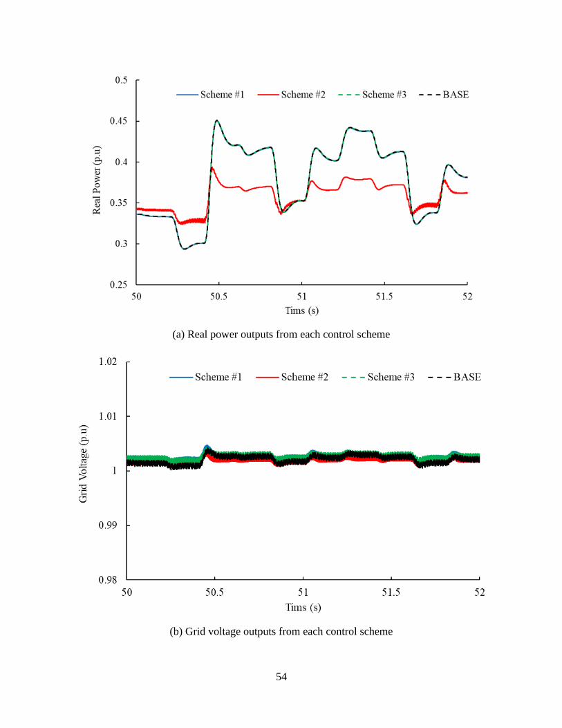
54
(a) Real power outputs from each control scheme
(b) Grid voltage outputs from each control scheme

55
(c) Reactive power outputs from each control scheme
Figure 4.3. Simulation results for each control scheme when SCR = 25 and X/R ratio = 15
In both Figures 4.2 and 4.3, the black dash line, solid blue line, solid red line, and green
dash line represent the base control without any mitigation techniques, VAR control, BESS
control, and adaptive control, respectively. In Figure 4.2, the hydrokinetic power plant with the
weak grid condition within the low X/R ratio network is manipulated, and the grid voltage shows
very severe voltage flicker in the short-term view; however, in Figure 4.3, the grid condition is
stiff with the high X/R ratio, so the grid voltage is not easily disturbed by the real power
fluctuation caused by the water turbulence unlike Figure 4.2. Both real power outputs in Figures
4.2 and 4.3 are affected by the same water turbulence intensity; the grid voltage outputs in two
different grid conditions indicate that the weak grid and low X/R ratio induce more severe
voltage flicker. According to the results in Figure 4.2(b), the VAR control seems not so much
effective to mitigate flicker by comparison with the base control (i.e., no flicker mitigation

56
control); therefore, the reactive power compensation is very limited to mitigate flicker in the
weak grid with the low X/R ratio.
As mentioned earlier, it is difficult to assess flicker severity by the graphs objectively.
Hence, the quantification of flicker in the short-term, Pst is measured in each different grid
condition to objectively compare the efficiency of each control scheme for flicker mitigation.
Table 2 shows Pst of each control scheme within the stiff grid (SCR = 25) with the three different
X/R ratios (X/R ratios = 15, 2, 1.025). Table 3 demonstrates Pst of each control scheme within
the weak grid (SCR = 6) with the three different X/R ratios (X/R ratios = 15, 2, and 1.025).
According to Tables 2 and 3, the values of the Pst increase as SCR and X/R ratio of the
grid decrease; it can verify that flicker in the power grid of the tidal power plant becomes severe
when the SCR and X/R ratio is small. The standard IEC 61000-3-7 specifies observation
intervals for flicker and the “compatibility level” for Pst as 1.0 for 10 minutes, and Pst that is
greater than 1 indicates a relatively high perceptible probability of a flicker problem [39]. This
case study assumes this compatibility level as a voltage quality reference point even though the
compatibility levels for MV or HV systems are not specifically defined by IEC standards [39].
Therefore, in the weak grid with the low X/R ratio (low impedance angle of the grid), the
VAR control has a limit to mitigate flicker. Still, the VAR control can moderately mitigate
flicker when the X/R ratio is large regardless of the SCR. With the BESS and adaptive Iq – V
control, flicker is effectively mitigated even when the X/R ratio is small. The BESS control is the
most effective way to mitigate flicker among the control schemes regardless of the SCR and X/R
ratio, but it is least cost-effective and might need extra space for deployment of the BESS
system. The adaptive control can also effectively mitigate flicker in every grid situation;
however, the rated current of the IGBTs on the GSC should be large enough to inject a large

57
amount of the reactive current Iq when flicker is very severe with the poor grid condition. So, it
also indicates that the size of the IGBTs and its corresponding costs for the power inverters
should be considered too. Therefore, the control schemes should be determined by the grid status
and cost. Figure 4.4 demonstrates the bar graphs for the summary of the results in Table 2 and
Table 3.
Table 2. Pst in the stiff grid
Table 3. Pst in the weak grid
SCR = 6 (Weak grid)
Control Pst (X/R=15) Pst (X/R=2) Pst (X/R=1.025)
Base 0.3981 0.6027 1.0610
VAR 0.3292 0.4572 0.9754
BESS 0.2671 0.3576 0.4435
Adaptive 0.2883 0.3968 0.5201
SCR = 25 (Stiff grid)
Control Pst (X/R=15) Pst (X/R=2) Pst (X/R=1.025)
Base 0.1763 0.2461 0.2926
VAR 0.1675 0.2312 0.2738
BESS 0.1523 0.1817 0.1891
Adaptive 0.1541 0.2071 0.2074

58
Figure 4.4. Summary of the results in case 1
4.3. Case 2: Varied Water Turbulence with Fixed SCR and X/R Ratio.
In this case scenario, the water turbulence is varied by changing the turbulence
intensity %TI, but the SCR and X/R ratio which determines the grid condition are fixed to test
the effectiveness of each flicker mitigation technique when the real power fluctuation caused by
the water turbulence in the hydrokinetic power generation becomes greater or smaller. In order to
assess Pst with the varied water turbulence in each different control scheme, the SCR is set to 6,
and the X/R ratio is fixed to 2, so the differentiated values of Pst can be observed based on the
different water turbulence.
Figures 4.5 and 4.6 demonstrate the water speeds, real power outputs of the MHK power
generation, and the voltage at the grid with the water turbulence 7.2% and 11.6% for each
control scheme. Compared with the real power fluctuation in Figures 4.2 and 4.3, the real power
fluctuation and grid voltage fluctuation becomes more severe in Figures 4.5 and 4.6.

59
(a) Water speed with %TI = 7.2%
(b) Real power outputs of each control scheme

60
(c) Grid voltage outputs of each control scheme
Figure 4.5. Simulation results for each control scheme when %TI = 7.2%
(a) Water speed with %TI = 11.6%

61
(b) Real power outputs of each control scheme
(c) Grid voltage outputs of each control scheme
Figure 4.6. Simulation results for each control scheme when %TI = 11.6%

62
As shown in Figures 4.5 and 4.6, the real power fluctuation and grid voltage fluctuation
become more severe as the water turbulence intensity becomes greater. Therefore, water
turbulence also should be considered when flicker mitigation techniques are determined. Since
the graphs of the grid voltage in Figures 4.5 and 4.6 cannot be objectively assessed to compare
the effectiveness of mitigating flicker for each control scheme, the short-term flicker severity Pst
is calculated again, and the results of Pst for each control scheme with the varied turbulence
intensity are shown in Table 4. Figure 4.7 demonstrates the bar graphs of the summary for the
results in Table 4 to explain the results intuitively.
Table 4. Pst with different turbulence intensity
Figure 4.7. Summary of the results in case 2
SCR = 6 & X/R Ratio = 2
Control
Pst
(%TI = 3.2%)
(Moderate)
Pst
(%TI = 7.2%)
(Severe)
Pst
(%TI = 11.6%)
(Very Severe)
Base 0.6027 1.1228 1.9020
VAR 0.4572 0.9931 1.6456
BESS 0.3576 0.5229 0.6894
Adaptive 0.3968 0.6685 1.0196

63
Considering the limiting value for the acceptable Pst on the grid that is Pst = 1.0, when the
turbulence intensity of the water flow is very severe, the voltage fluctuation is mainly caused by
the fluctuation of the real power. The very severe turbulence intensity (i.e., %TI = 11.6% in the
case study), of course, is unlikely to happen in the river and sea because the turbulence intensity
of the water flow in the river is not easily changed; however, with consideration of the worst
water turbulence situation, the BESS, which smooths the real power fluctuation out of the tidal
power generator (by discharging and charging the amount of the fluctuating real power), might
be the best way to mitigate flicker and satisfy the grid code in the area that the tidal power plant
is installed. The adaptive control is advantageous to mitigate flicker when the water turbulence is
moderate or severe, and it does not require extra cost for implementation of the additional
hardware into the system, unlike the BESS. Since the size of the GSC (rated currents of the
IGBTs) is limited in the simulation, the simulation results also reflect the limit of flicker
mitigation when the water turbulence is very severe, meaning that the reactive current Iq needs
more to be injected into the system. Reactive power compensation is easy to implement, but it is
limited to mitigate flicker when the X/R ratio of the grid is too low. Therefore, based on grid
conditions and the water flow characteristics in the areas where the tidal power plant is installed
and the budget, the control scheme of flicker mitigation should be decided. Eventually, the tidal
power plant can be integrated into the system by promising the stabilized grid voltage and
improved power quality.

64
5. Conclusion and Future Work
5.1 Conclusion
This thesis proposes a tidal and river MHK power generation model to study the effect of
the operational condition of hydrokinetic power (i.e., water turbulence intensity) and grid
parameters (i.e., SCR & X/R ratio) on flicker, and to explore the three different control schemes
(i.e., reactive power control, use of the BESS, and adaptive Iq – V control) to provide flicker
mitigation. The case study and the simulation modeling are performed by PSCAD, which is a
dynamic power system software. In order to objectively assess flicker severity in each control
scheme and quantify the level of flicker severity, the short-term flicker severity Pst is calculated
by the flickermeter tool in MATLAB/SIMULINK.
In the theoretical model of the MHK power generation for the digital simulation, the
modeling of the PMSG and the hydrokinetic turbine is described, and their mathematical model
and MPPT control of the hydrokinetic turbine are explained. The output results of the machine
side (PMSG and hydrokinetic turbine) based on the variable water speed are shown in the graph.
Then, the electrical power conversion throughout the back-to-back power converter consisting of
the diode rectifier, DC-DC boost converter, and DC-AC inverter and their control schemes are
described in Chapter 2.4. Based on the theoretical model of the MHK power generation, the three

65
different control schemes for flicker mitigation are implemented on the system model, and the
case studies with the varied water turbulence and varied grid parameters are conducted.
According to the results in the first case study, the BESS and adaptive control effectively
mitigate flicker regardless of the X/R ratio, but the VAR control can mitigate flicker only at a
certain level of X/R ratio in the weak grid. In the second case study, the real power fluctuation
becomes varied by changes in the water turbulence; the BESS that smooths real power
fluctuation has the most effective results, and the other two control techniques that use the
reactive components have a limit to mitigate flicker when the water turbulence is too severe. As
previously mentioned, the implementation of the dedicated storage to the power system is less
financially viable than implementing the control logic into the converters; however, in the case
of the distribution network with the very weak power system and very severe water turbulence
(low impedance angle and very weak grid condition), the BESS can be an adequate decision to
mitigate flicker in the tidal and river power generation. But, in the case of the weak grid
conditions and severe water turbulence, the adaptive control is the optimal choice to stabilize the
voltage fluctuation since it does not require the extra cost and space for implementation, unlike
the BESS. Of course, the current capacity (rated current) of the inverters in GSC should be
considered when the hydrokinetic system is built. If the distribution network has slightly weak
and relatively high X/R ratio, such as distribution network that has a long radial power line, the
VAR control in GSC is enough to be used to stabilize the grid voltage and flicker, but the line
resistance and line reactance of the grid system must be known when the VAR control is used.
Therefore, the mitigation techniques shall be considered based on the types of the grid
connection and the water flow characteristics in the areas where the tidal power plant is installed,
considering the cost.

66
5.2 Future Work
The hardware design for verification of the software simulation will be presented in
Appendix 1. The main objective of the hardware simulation is to reproduce the hydrokinetic
dynamic behavior with the MHK power system and verify the results of the digital simulation.
The connection overview of the hardware design will be provided, and the basic model of the
induction motor with the VFD, which represents the hydrokinetic turbine, will be explained.
Only the induction motor with the VFD and synchronous generator connected to the induction
motor with the mechanical shaft are set up now; hence, the rest of the hardware parts such as a
microcontroller and power converters to the grid will be handled as future work. The details of
the hardware design of the MHK power system that has been completed and will be completed
are presented in Appendix 1.

67
References
[1] M. Mason, “Renewable energy: All you need to know,” Esyoh, LLC, 9 November 2016.
[Online]. Available: https://www.environmentalscience.org/renewable-energy. [Accessed: 16
June 2020]
[2] E. Muljadi, A. Wright, V. Gevorgian, J. Donegan, C. Marnagh, and J. McEntee, “Power
generation for river and tidal generators,” National Renewable Energy Laboratory (NREL).
[Online]. Available: http://www.nrel.gov/docs/fy16osti/66097.pdf. [Accessed: 16 June 2020]
[3] “Data and Statistics,” International Energy Agency (IEA), 12 April 2018. [Online].
Available: https://www.iea.org/data-and-statistics. [Accessed: 16 June 2020].
[4] K. Kilcher, R. Thresher, H. Tinnesand, “Marine Hydrokinetic Energy Site Identification and
Ranking Methodology Part I: Tidal Energy,” National Renewable Energy Laboratory (NREL),
Golden, CO, USA, 2016.
[5] A. Owen, M.L. Trevor, “Tidal Current Energy: Origins and Challenges,” in Future Energy,
pp. 111-128, 2008.
[6] R. A.R. Tricker, P. Groen, “Tide,” Encyclopædia Britannica, 20 February 2020. [Online].
Available: https://www.britannica.com/science/tide. [Accessed: 16 June 2020].
[7] H. J. Yadav, “Recent developments of Ocean Energy in India – An Overview,” in
International Journal on Recent and Innovation Trends in Computing and Communication, vol.
3, no. 12, pp. 6717 - 6721, Dec. 2015.
[8] “IEEE Recommended Practice for the Analysis of Fluctuating Installations on Power
Systems," in IEEE Std 1453-2015 (Revision of IEEE Std 1453-2011), vol., no., pp.1-74, 30 Oct.
2015.
[9] C. V. Moreno, H. A. Duarte, and J. U. Garcia, "Propagation of flicker in electric power
networks due to wind energy conversions systems," in IEEE Transactions on Energy
Conversion, vol. 17, no. 2, pp. 267-272, June 2002.
[10] A. Baggini, “Handbook of Power Quality,” New York: Wiley, 2008.
[11] “Electromagnetic Compatibility (EMC)-Part 4: Testing and Measurement Techniques-
Section 15: Flickermeter – Functional and Design Specifications,” in IEC Std. 61000-4-15,
November 1997.

68
[12] J. C. Gomez and M. M. Morcos, "Flicker Measurement and Light Effect," in IEEE Power
Engineering Review, vol. 22, no. 11, pp. 11-15, Nov. 2002.
[13] J. MacEnri, M. Reed, and T. Thiringer, "Influence of Tidal Parameters on SeaGen Flicker
Performance," European Wave and Tidal Energy Conference (EWTEC), Southampton, UK,
2011.
[14] S. Walker and L. Cappietti, “Experimental Studies of Turbulent Intensity around a Tidal
Turbine Support Structure,” Energies, vol. 10, pp. 497, 2017.
[15] W. Hu, Z. Chen, Y. Wang, and Z. Wang, “Flicker mitigation by active power control of
variable-speed wind turbines with full-scale back-to-back power converters,” in IEEE Trans.
Energy Convers., vol. 24, no. 3, pp. 640–649, Sep. 2009.
[16] M. Ammar and G. Joos, “A short-term energy storage system for voltage quality
improvement in distributed wind power,” IEEE Trans. Energy Convers., vol. 28, no. 2, pp. 425–
433, Dec. 2014.
[17] F. Diaz-Gonzalez, F. Bianchi, A. Sumper, and O. Gomis-Bellmunt, “Control of a flywheel
energy storage system for power smoothing in wind power plants,” IEEE Trans. Energy
Convers., vol. 29, no. 1, pp. 204–214, Mar. 2014.
[18] M. Ammar and M. E. Ammar, "Enhanced Flicker Mitigation in DFIG-Based Distributed
Generation of Wind Power," in IEEE Transactions on Industrial Informatics, vol. 12, no. 6, pp.
2041-2049, Dec. 2016.
[19] M. Ammar and G. Joos, “Impact of distributed wind generators reactive power behavior on
flicker severity,” IEEE Trans. Energy Convers., vol. 28, no. 2, pp. 425–433, Jun. 2013.
[20] T. L. Van, T. H. Nguyen and D. Lee, "Flicker mitigation in DFIG wind turbine systems,"
Proceedings of the 2011 14th European Conference on Power Electronics and Applications,
Birmingham, U.K., pp. 1-10, 2011.
[21] Y. Jiang, M. F. Rong and L. Y. Hua, "Variable speed constant frequency tidal current
energy generation and control strategy for maximum power point tracking and grid
connection," 2009 International Conference on Sustainable Power Generation and Supply,
Nanjing, China, pp. 1-6, 2009.
[22] M. J. Khan, T. Iqbal, and J. E. Quaicoe, “River current energy conversion systems:
Progress, Prospects and Challenges,” Renewable and Sustainable Energy Reviews. 2008.
[23] Ocean Renewable Power Company, [Online]. Available: https://www.orpc.co. Portland,
Maine. [Accessed: 20 June 2020]
[24] N. Goudarzi and D. Zhu, "A review on the development of wind turbine generators across
the world," International Journal of Dynamics and Control, vol. 1, pp. 192-202, 2013.

69
[25] M. Liu, “Hydrokinetic turbine power converter and controller system design and
implementation,” Master Thesis, Vancouver, Canada: University of British Columbia, Aug.
2014.
[26] P.M. Anderson and A.A. Fouad, “Power System Control and Stability,” Piscataway, N.J.:
IEEE Press; Wiley-Interscience, 2003.
[27] J. Khan, “A generic performance curve for tidal and hydrokinetic devices,” Journal of
Ocean Technology, vol. 13. pp. 54-62, 2018.
[28] Y. Song, Y. Chen, S. Huang, Z. Yu and Y. Qiao, "Average value model of grid side
converter in PMSG for system-level studies," in The Journal of Engineering, vol. 2017, no. 13,
pp. 1799-1803, 2017.
[29] G. Shi, M. Zhu, X. Cai, Z. Wang, and L. Yao, "Generalized average model of DC wind
turbine with consideration of electromechanical transients," IECON 2013 - 39th Annual
Conference of the IEEE Industrial Electronics Society, Vienna, pp. 1638-1643, 2013.
[30] T. Sun, Z. Chen, and F. Blaabjerg, "Flicker study on variable speed wind turbines with
doubly fed induction generators," in IEEE Transactions on Energy Conversion, vol. 20, no. 4,
pp. 896-905, Dec. 2005.
[31]Y. Song, Y. Chen, S. Huang, Z. Yu and Y. Qiao, "Average value model of grid side
converter in PMSG for system-level studies," in The Journal of Engineering, vol. 2017, no. 13,
pp. 1799-1803, 2017.
[32] A. Burke, H. Zhao, "Applications of Supercapacitors in Electric and Hybrid Vehicles,"
Research Report - UCD-ITS-RR-15–09, vol. 15, 2015.
[33] A. Vassallo, P. Maker, T. Dixon, and V. Agelidis, "Electricity Storage: Renewable Energy
Applications in the Australian Context," in IEEE Electrification Magazine, vol. 3, no. 3, pp. 22-
29, Sept. 2015.
[34] H. Hesse, M. Schimpe, D. Kucevic, and A. Jossen, “Lithium-Ion Battery Storage for the
Grid—A Review of Stationary Battery Storage System Design Tailored for Applications in
Modern Power Grids,” Energies, vol. 10, pp. 2107, 2017.
[35] O. Tremblay and L. A. Dessaint, “Experimental Validation of a Battery Dynamic Model for
EV Applications,” World Electric Vehicle Journal, vol. 3, pp. 289-298, 2009.
[36] J. Kim, E. Muljadi, J. Park and Y. C. Kang, "Flexible IQ–V Scheme of a DFIG for Rapid
Voltage Regulation of a Wind Power Plant," in IEEE Transactions on Industrial Electronics,
vol. 64, no. 11, pp. 8832-8842, Nov. 2017.
[37] J. D. Lavers and P. P. Biringer, "Real-Time Measurement of Electric Arc-Furnace
Disturbances and Parameter Variations," in IEEE Transactions on Industry Applications, vol.
IA-22, no. 4, pp. 568-577, July 1986.

70
[38] N. P. W. Strachan and D. Jovcic, "Stability of a Variable-Speed Permanent Magnet Wind
Generator With Weak AC Grids," in IEEE Transactions on Power Delivery, vol. 25, no. 4, pp.
2779-2788, Oct. 2010
[39] “IEEE Guide--Adoption of IEC/TR 61000-3-7:2008, Electromagnetic compatibility (EMC)-
-Limits--Assessment of emission limits for the connection of fluctuating installations to MV, HV
and EHV power systems," in IEEE Std 1453.1-2012 (Adoption of IEC/TR 61000-3-7:2008), vol.,
no., pp.1-78, 6 July 2012.
[40] P.C. Sen, “Principles of electric machines and power electronics,” Chichester, England:
John Wiley & Sons, 1997.

71
Appendix 1. Future Work - Hardware Simulation for Verification
In Appendix 1, the hardware model and emulation for the hydrokinetic power generation
are presented. The main objective of the hardware simulation is to reproduce the hydrokinetic
dynamic behavior implemented in the microcontroller sending the reference speed to the
Variable Frequency Drive (VFD), and the VFD connected to the wound rotor induction motor
emulates the variable speed of the tidal turbine. Then, the induction motor that mimics the tidal
turbine is connected to the synchronous generator to provide the electrical energy to the grid
system. As soon as the hardware simulation is ready to be set up, the verification of the software
simulation will proceed to compare the results of the hardware simulation manipulating the
voltage flicker on the grid system with the software simulation as future work. Figure A.1
demonstrates the overview of the hardware connection for emulating the hydrokinetic power
generation.
Figure A.1. Connection overview of the hardware simulation

72
As shown in Figure A.1, the VFD will control the speed of the induction motor based on the
hydrokinetic dynamic model on the interface (i.e., PC), and the microcontroller transmits the
reference speed to the VFD as an analog signal. The microcontroller helps to exchanges the
analog and digital signal between the interface and the hardware such as VFD and motor; it
collects analog signals from the motor or power converters and uses them to calculate the
reference speed for VFD to emulate the variable speed of the induction motor, which mimics the
hydrokinetic turbine. With the given tidal turbine parameters and the specified water speed, the
software interface provides the corresponding reference speed for the induction motor
throughout the VFD control to emulate the tidal turbine. The next subsection explains the set-up
for the induction motor connected to the VFD and the control scheme of the VFD to enable the
induction motor operating in the variable speed. Until now, the only induction motor and VFD
are tested to operate them as a variable speed motor, and the microcontroller, synchronous
generator, and power converters with the grid simulator will be set up as future work in this
report. Table 5 indicates the specification of the hardware components that will be used in the
hardware simulation. The circuit parameters (resistance and inductance of stator and rotor) of the
induction motor are not listed in the table because their values are not indicated on the
nameplate, and the manual for the machine does not exist (the model is too old to find the
manual). Therefore, the no-load test and blocked-rotor test are required to find the circuit
parameters of the induction motor later on.

73
Table 5. Specification of hardware simulation
Induction Motor
Horsepower 10 HP
Rated Power 7.457 kW
Rate Speed 1735 RPM
Number of Pole Pairs 2
Input Voltage (Y-Δ) 230 (Low) / 460 (High) V
Rated Current 30 (Low) / 15 (High) A
Frequency 60 Hz
Synchronous Generator
Rated Power 7.5 kW
Rated Frequency 60 Hz
Power Factor 0.8
Rated Speed 1800 RPM
Voltage 240 (Low) / 480 (High) V
Rated Current 23 (Low) / 11 (High) V
VFD
Input Voltage 220 ± 15% Vac Output Voltage 0 ~ Rated Input Voltage
Input Frequency 47 ~ 63 Hz
Output Frequency 0 ~ 400 Hz
Rated Power 7.5 kW
Rated Output Current 34 A
Instead of building the real hydrokinetic turbine with the water flow, the variable speed
of the induction motor controlled by the VFD will emulate the hydrokinetic turbine in this
hardware simulation. The picture of the induction motor connected to the VFD and synchronous
generator in the power laboratory is shown in Figure A.2.

74
Figure A.2. Picture of the induction motor, synchronous generator, and VFD
Before presenting the VFD functionality, the characteristics of the induction motor and
its speed control with the V/F control implemented in the VFD should be explained to
understand the control scheme of the VFD. It is essential to understand the characteristics of the
induction motor in order to explain the use of the VFD that makes the induction motor emulating
the hydrokinetic turbine as a variable speed drive. The equivalent circuit of the induction motor
is shown in Figure A.3.

75
Figure A.3. Equivalent circuit of the induction machine
The induction machine, or asynchronous machine, has a stator side and a rotor side,
mainly. Both stator winding and rotor winding carry alternating currents, and the AC is supplied
to the stator winding and rotor winding by induction. The details of the induction machine and its
mechanisms are explained in the literature [40]. In this section, the basic derived equations for
the running operation in the induction machine and the speed control for the induction motor are
presented. Referencing to Figure A.3, if the stator windings are connected to a three-phase
supply (VFD in this simulation), and the rotor circuit is closed, the induced voltages in the rotor
side produce the rotor currents. These rotor currents interact with the air gap field to produce the
torque, and then the rotor starts rotating because of the relative speed difference between the
rotating field and the rotor winding. In the induction machine, there are no induced voltages,
currents, and torques at nr = nsync. Therefore, the slip s that is the difference between nr and nsync
is a very significant factor in understanding the running operation of the induction machine, and
the slip is defined as:

76
𝑠 =𝑛𝑠𝑦𝑛𝑐 − 𝑛𝑟
𝑛𝑠𝑦𝑛𝑐 (𝐴. 1)
Therefore, in order to rotate the rotor of the induction motor, the slip should be greater or less
than 0 instead of being equal to zero (nr = nsync). The relative speed between the rotating field and
the rotor winding should exist to rotate the machine in the induction motor. Then, the slip
frequency fr of the induced voltage and the current in the rotor circuit will correspond to this slip
rpm (nsync – nr = s nsync) because this is the relative speed between the rotating field and the rotor
winding. The rotor circuit frequency fr can be written as:
𝑓𝑟 =𝑝
120(𝑛𝑠𝑦𝑛𝑐 − 𝑛𝑟) =
𝑝
120𝑠𝑛𝑠𝑦𝑛𝑐 = 𝑠𝑓𝑠 (𝐴. 2)
where p is the number of poles, and fs is the stator circuit frequency (frequency of the supply).
Then, the induced currents in the rotor windings also produce a rotating field, and its speed in
RPM with respect to the rotor (represent the speed of the motor, usually) is:
𝑛 = 120 ∗𝑓𝑟𝑝
= 120 ∗𝑠𝑓𝑠𝑝
= 𝑠 𝑛𝑠𝑦𝑛𝑐 (𝐴. 3)
Unlike the synchronous generator, as explained in chapter 2.3, the induction motor has a slip,
and the slip is an important factor in expressing the speed of the induction machine.
As shown in Figure A.3, the equivalent circuit of the induction motor consists of the stator
winding part and rotor winding part. In Figure A.3, the stator winding can be represented, where:
Vs = per-phase terminal voltage in stator side
Rs = per-phase stator winding resistance
Xs = per-phase stator leakage inductance
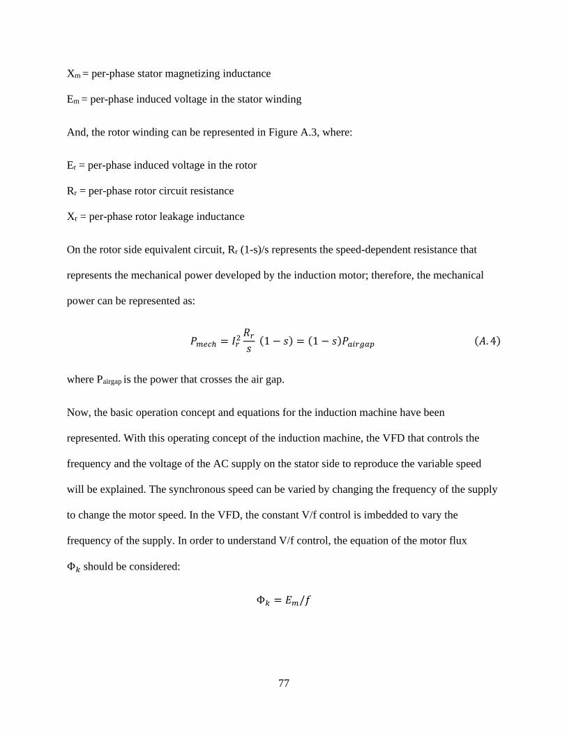
77
Xm = per-phase stator magnetizing inductance
Em = per-phase induced voltage in the stator winding
And, the rotor winding can be represented in Figure A.3, where:
Er = per-phase induced voltage in the rotor
Rr = per-phase rotor circuit resistance
Xr = per-phase rotor leakage inductance
On the rotor side equivalent circuit, Rr (1-s)/s represents the speed-dependent resistance that
represents the mechanical power developed by the induction motor; therefore, the mechanical
power can be represented as:
𝑃𝑚𝑒𝑐ℎ = 𝐼𝑟2𝑅𝑟
𝑠 (1 − 𝑠) = (1 − 𝑠)𝑃𝑎𝑖𝑟𝑔𝑎𝑝 (𝐴. 4)
where Pairgap is the power that crosses the air gap.
Now, the basic operation concept and equations for the induction machine have been
represented. With this operating concept of the induction machine, the VFD that controls the
frequency and the voltage of the AC supply on the stator side to reproduce the variable speed
will be explained. The synchronous speed can be varied by changing the frequency of the supply
to change the motor speed. In the VFD, the constant V/f control is imbedded to vary the
frequency of the supply. In order to understand V/f control, the equation of the motor flux
Φ𝑘 should be considered:
Φ𝑘 = 𝐸𝑚/𝑓

78
where E is the induced voltage on the stator winding, and f is the frequency of the supply. Since
the voltage drop across Rs and Xs is small compared to the terminal voltage of the stator side Vs,
so Vs = Em So, the motor flux can be rewritten as:
Φ𝑘 = 𝑉/𝑓
Therefore, in order to change the speed, the terminal voltage of the motor is varied as the
frequency of the supply changes proportionally. This control is called “constant volts per hertz.”
To maintain the constant air gap flux density, the required variation of the supply voltage with
the frequency should exist, as shown in Figure A.4.
Figure A.4. V/f pattern for the constant volts per hertz control in the induction machine
With this V/f control, the VFD control scheme is shown in Figure A.5 with the hydrokinetic
dynamic model.

79
Figure A.5. VFD control scheme with hydrokinetic dynamics
In Figure A.5, the hydrokinetic dynamics are already explained in the previous chapter
2.3; the VFD requires the reference frequency in proportion to the voltage representing the
corresponding reference speed obtained from the hydrokinetic dynamics. 𝜔𝑒 represents the
reference synchronous speed obtained from the reference speed of the turbine (𝜔𝑟𝑒𝑓) from the
MPPT of the hydrokinetic dynamic. Therefore, the induction motor operates in the reference
frequency based on the reference speed of the hydrokinetic dynamics. The induction motor
emulates the hydrokinetic turbine following the hydrokinetic dynamics embedded in the
interface (i.e., PC and microcontroller). Figure A.6 also demonstrates the VFD equivalent circuit
with the connected AC source and the induction motor. As shown in Figure A.6, the topology for
the VFD circuit is very similar to the back-to-back converter; the AC source is converted to the
DC throughout the diode rectifier (AC-DC), and the PWM control signals for the VFD control as
shown in Figure A.5 are carried to the inverters on the right side to control the speed of the
induction machine throughout the DC-AC inverter. The control circuit for generating the PWM
is embedded in the VFD. Therefore, the VFD controls the input frequency and the voltage of the

80
induction motor in order to control the motor speed, eventually. So, the induction motor
controlled by the VFD can emulate the tidal turbine, including the hydrokinetic dynamics,
according to the above explanation.
Figure A.6. The equivalent circuit for the VFD connected to the induction motor
Then, the induction motor controlled by the VFD is directly connected to the synchronous
generator with the shaft coupling (mechanically direct coupled), and its mechanical coupling
reflects the equation of the mechanical model in equation (2.13).
The hardware design that is set up now is the induction motor with the VFD and synchronous
generator connected to the induction motor. The rest of the system will be discussed in future
work.
For the hardware simulation, the only tidal turbine (induction motor and VFD) part is
operated and tested. The synchronous generator is connected to the induction motor with direct
shaft coupling. However, the power converters connection and grid system simulator are not set
up yet. According to the software model of the hydrokinetic power generation, the power
converter should consist of:

81
1. The AC-DC diode rectifier to convert the variable AC of the synchronous generator
into the variable DC.
2. The DC-DC converter to control the DC voltage, maintaining the output power based
on the MPPT control.
3. The DC-AC inverter to implement the GSC controls or the corresponding flicker
mitigation control schemes and DC-link constant.
Then, the grid simulator existed in the power laboratory (NHR - 9410 model) will be connected
to the output of the DC-AC inverter, so the hardware system can operate as similar to the digital
simulation and verify the results obtained from the digital simulation.