Marked Tableaux

By

Graham Hawkes

DISSERTATION

Submitted in partial satisfaction of the requirements for the degree of

DOCTOR OF PHILOSOPHY

in

MATHEMATICS

in the

OFFICE OF GRADUATE STUDIES

of the

UNIVERSITY OF CALIFORNIA

DAVIS

Approved:

Anne Schilling (chair)

Eugene Gorskiy

Monica Vazirani

Committee in Charge

2019

-i-

Pro Libertate

-ii-

Contents

Abstract v

Acknowledgments vi

Chapter 1. Introduction 1

Chapter 2. Primed and Signed Tableaux of Straight Shape: Double Stanley Symmetric Functions 3

2.1. Introduction 3

2.2. Primed Signed Tableaux 6

2.3. Littlewood-Richardson Rules 10

2.4. Double Stanley Symmetric Functions 15

2.5. Signed-insertion 17

2.6. Conjectures 24

Chapter 3. Primed and Signed Tableaux of Shifted Shape: Type C Stanley Symmetric Functions 27

3.1. Introduction 27

3.2. Crystal isomorphism 28

3.3. Explicit crystal operators on shifted primed tableaux 35

3.4. Signed tableaux of shifted shape: Semistandard unimodal tableaux 40

Chapter 4. Marked Tableaux of Staircase Shape: The Schur function sδ/µ 43

4.1. Introduction 43

4.2. Definitions 44

4.3. Results 45

Chapter 5. Primed Tableaux of Shifted Shape Revisited: Crystal Characterization 50

5.1. Introduction 50

5.2. Queer supercrystals 51

-iii-

5.3. Local axioms 53

5.4. Graph on type A components 57

5.5. Characterization of queer crystals 59

Appendix A. Appendix 1: Proofs for Type A crystal on primed tableaux 60

A.1. 60

A.2. 70

Appendix B. Appendix 2: Proofs for characterization of queer crystals 75

B.1. 75

B.2. 78

Bibliography 92

-iv-

Graham HawkesJune 2019

Mathematics

Marked Tableaux

Abstract

This dissertation is an exploration of tableaux that may be formed using entries from the ordered alpha-

bet X′ = · · · < 2 < 1 < 1′ < 1 < 2′ < 2 < · · · and the symmetric functions and crystal structures that are

related to them.

These ”marked tableaux,” have had, have in this paper, and undeniably will continue to have profound

impacts in the areas of Schur and P-Schur positivity, Stanley symmetric functions, Grothendieck polynomi-

als, crystal bases, and the theory of jeu de taqin.

We will find that for each of the Stanley symmetric functions which have been historically or currently

considered there is a corresponding type of marked tableaux. These tableaux will represent certain connected

components on what we see as natural crystal structures for Stanley symmetric functions. Then, we will

analyze the nature of two types of marked tableaux in greater detail: marked staircase shape tableaux, and

primed shifted tableaux.

-v-

Acknowledgments

I’d like to thank a few math professors from my undergraduate time at UNC whose authenticity and

dedication to their profession inspired me to continue this path. Foremost among these are my undergrad-

uate advisor, Justin Sawon, as well as three more professors who stood out markedly in professionalism,

generosity, and good humour: Ellen Eischen, Robert Proctor, and Karl Petersen.

I’d like to thank Sarah Driver. Because she does her job well (even when I do my job poorly) and she

does it smiling (even when I do my job poorly). Of course, I’d like to thank Tina and the rest of the office

staff as well. Although I have had less personal interaction with them, their jobs are just as essential to keep

the department functioning.

I’d like to thank my fellow graduate students for words of encouragement and advice. I’d like to thank

them for the company they have provided over the last five years, and the illusion of normalcy that the

absurdity of each of our situations has bestowed upon the others. In particular, I’d like to thank my friends

and office mates John Challenor and Tynan Lazarus.

I’d like to thank my advisor Anne Schilling. For many things: For being genuinely concerned about my

academic (and general) well-being. For never forgetting about a single email I have sent her (there were a

lot). For giving me good problems to work on. For being incredibly available even at her busiest to discuss

these problems. For always being (counterexample thieves aside) calm-headed, rational, and fair. For always

putting others before herself. But most of all for believing in me, for trusting in me, and for treating me like

a colleague.

I’d like to thank her along with the rest of my committee, Eugene Gorskiy and Monica Vazirani for their

service on my qualifying exam committee, the letters of reference they have written me (apparently good

ones), and their willingness to serve on this committee.

I’d like to thank my family. My father, for his sense of humour and his strength. And for pretending

that having read a few math books makes me smart. My mother, for her compassion and her understanding.

And for helping me to learn to love computers. My brother, for his kindness and his intelligence. And for

teaching me all the things he didn’t mean to. My sister, for her heart, and for her heart again. And for

teaching me to never give up.

-vi-

CHAPTER 1

Introduction

We consider the alphabet X′ = · · · < 2 < 1 < 1′ < 1 < 2′ < 2 < · · · . A valid tableau is formed

using these entries if its rows and columns are weakly increasing, its columns contain no repeated unmarked

entries, and its rows contain no repeated marked entries. Such tableaux are the central theme of all that

follows.

The work is structured as follows. The first part analyzes straight-shape marked tableaux. These marked

tableaux are the natural generalization of straightshape semistandard Young tableaux. Closely related to this

concept is the concept of a double Stanley function which is the analogous generalization of the type A

Stanley symmetric function. The main result of this section about the double Schur positivity of the double

Stanley symmetric function (see Theorem 4.3.1). The work in this part is based on a paper, [Haw18], written

by the current author.

The second part analyzes primed tableaux of a shifted shape. Continuing our analogy these tableaux

correspond to the type C Stanley symmetric function. There is also a mention of semistandard unimodal

tableaux in this part. One may object that (as we will see) these tableaux do not contained marked entries but

are rather defined (in part) by having rows composed of hook words (that is, which at first strictly descend

and then weakly ascend). However this condition is equivalent (up to a power of 2 to the number of rows) to

the condition that the rows are made up of barred and unmarked entries. Thus the relation between primed

and signed tableaux played in the straightshape case is analogous to the relationship between shifted primed

tableaux and semistandard decomposition tableaux in the shifted shape case. The main takeaway here is

the relationship between a crystal structure and an insertion algorithm of Haiman: this is made precise in

Theorem 3.3.3 as well as the Schur expansion for the type c Stanley which falls out as a result. This part is

based on portions of a [HPS17] coauthored by Kirill Paramanov and Anne Schilling. However, the theorems

and proofs which are included were originally written by the author himself.

The third part consists in analyzing a third type of tableaux. In this setting we are working with only

one type of marked entry, which would be best considered as primed entries. Here we have the additional

1

condition that we have some fixed index set that tells us for each i whether we may use unmarked or marked

entries. These tableaux will only be of interest for the staircase shape (although we also may consider skew

staircase shapes). Here the relation to symmetric functions is found by comparing the interchanging of

marked and unmarked entries to the interchanging of elementary and homogeneous symmetric functions.

This part is based on a [Haw17].

The final part is of a slightly different nature: It does not relate directly to marked tableaux but analyzes

the crystal structure that the set of shifted primed tableaux (or equivalently the set of semistandard unimodal

tableaux) affords from an abstract standpoint. The goal is to give a characterization of the more general

object whose character corresponds to that modeled by either of these types of tableau. This includes

portions of [GHPS18] coauthored with Maria Gillepsie, Wencin Poh, and Anne Schilling. The particular

parts that are included here represent primarily the mathematical work of the current author, although many

figures and examples were created or aided by other authors.

2

CHAPTER 2

Primed and Signed Tableaux of Straight Shape: Double Stanley Symmetric

Functions

This chapter is based on the work in [Haw18].

2.1. Introduction

Throughout this chapter, when some k ∈ N is specified x will refer to the list of variables (x1, . . . , xk) and

y will refer to the list of variables (y1, . . . , yk). On the other hand x will refer to the infinite list of variables

(x1, x2, . . .) and y will refer to the infinite list of variables (y1, y2, . . .). If the polynomial P(x) or P(x, y) is

defined for arbitrary k then P(x) or, respectively, P(x, y) will represent the corresponding function obtained

by letting k → ∞.

The An Coxeter system is defined as the Coxeter system with generators, s1, . . . , sn and relations (sis j)mi j =

1 where mi j is an integer determined as follows:

• If |i − j| = 0, mi j = 1.

• If |i − j| = 1, mi j = 3.

• If |i − j| > 1, mi j = 2.

By abuse of notation, we will also refer to the corresponding Coxeter group of size (n + 1)! as An. The

Cn Coxeter system is defined as the Coxeter system with generators, s0, s1, . . . , sn and relations (sis j)mi j = 1

where mi j is an integer determined as follows:

• If |i − j| = 0, mi j = 1.

• If i > 0 and j > 0, and |i − j| = 1, mi j = 3.

• If i = 0 or j = 0, and |i − j| = 1, mi j = 4.

• If |i − j| > 1, mi j = 2.

3

Similarly, we will sometimes refer to corresponding group of size 2n(n + 1)! itself as Cn. Given the

relations above one can define two types of symmetric functions, indexed, respectively, by elements of An

and Cn.

First, suppose ω ∈ An. A reduced word for ω is an expression, u, for ω using the generators s1, . . . , sn

such that no other such expression for ω is shorter than u. Given a fixed k, a reduced increasing k-

factorization (RIF), v, for ω is a reduced word u, for ω along with a subdivision of u into k parts such that

each part is increasing under the order s1 < · · · < sn. The weight of v is the vector whose ith entry records

the number of generators in the ith subdivision of v. The type A Stanley symmetric polynomial [Sta84] in k

variables for ω is:

FAω(x) =

∑v∈RIF(ω)

xwt(v),

where RIF(ω) is the set of reduced increasing k-factorizations of ω, and wt(v) is the weight of v. Letting

k → ∞ in the type A Stanley symmetric polynomial gives the type A Stanley symmetric function for ω.

Now suppose ω ∈ Cn. A reduced word for ω is an expression, u, for ω using the generators s0, s1, . . . , sn

such that no other such expression for ω is shorter than u. A reduced unimodal k-factorization (RMF), v,

for ω is a reduced word u, for ω along with a subdivision of u into k parts such that each part is unimodal

(i.e., decreasing and then increasing) under the order s0 < s1 < · · · < sn. The weight of v is the vector

whose ith entry records the number of generators in the ith subdivision of v. The type C Stanley symmetric

polynomial [BH95], [FK96], in k variables for ω is:

FCω(x) =

∑v∈U(ω)

2ne(v)xwt(v),

where ne(v) is the number of nonempty subdivisions of v, U(ω) is the set of reduced unimodal factorizations

of ω, and wt(v) is the weight of v. Letting k → ∞ in the type C Stanley symmetric polynomial gives the

type C Stanley symmetric function for ω.

4

Of course, for any ω ∈ An we may consider both FAω and FC

ω . Both functions are Schur positive, but

it is not exactly clear how the one relates to the other. To do this, we will define a third function Fdω. We

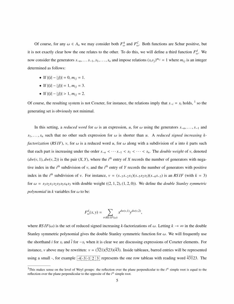
now consider the generators s−n, . . . s−1, s1, . . . , sn and impose relations (sis j)mi j = 1 where mi j is an integer

determined as follows:

• If |(|i| − | j|)| = 0, mi j = 1.

• If |(|i| − | j|)| = 1, mi j = 3.

• If |(|i| − | j|)| > 1, mi j = 2.

Of course, the resulting system is not Coxeter, for instance, the relations imply that s−i = si holds, 1 so the

generating set is obviously not minimal.

In this setting, a reduced word for ω is an expression, u, for ω using the generators s−n, . . . , s−1 and

s1, . . . , sn such that no other such expression for ω is shorter than u. A reduced signed increasing k-

factorization (RS IF), v, for ω is a reduced word u, for ω along with a subdivision of u into k parts such

that each part is increasing under the order s−n < · · · s−1 < s1 < · · · < sn. The double weight of v, denoted

(dw(v, 1), dw(v, 2)) is the pair (X,Y), where the ith entry of X records the number of generators with nega-

tive index in the ith subdivision of v, and the ith entry of Y records the number of generators with positive

index in the ith subdivision of v. For instance, v = (s−3s−2s1)(s−5s2s3)(s−4s−3) is an RS IF (with k = 3)

for ω = s3s2s1s2s3s5s4s3 with double weight ((2, 1, 2), (1, 2, 0)). We define the double Stanley symmetric

polynomial in k variables for ω to be:

Fdω(x, y) =

∑v∈RS IF(ω)

xdw(v,1)ydw(v,2),

where RS IF(ω) is the set of reduced signed increasing k-factorizations of ω. Letting k → ∞ in the double

Stanley symmetric polynomial gives the double Stanley symmetric function for ω. We will frequently use

the shorthand i for si and i for −si when it is clear we are discussing expressions of Coxeter elements. For

instance, v above may be rewritten: v = (321)(523)(43). Inside tableaux, barred entries will be represented

using a small -, for example -4 -3 -1 2 3 represents the one row tableau with reading word 43123. The

1This makes sense on the level of Weyl groups: the reflection over the plane perpendicular to the ith simple root is equal to thereflection over the plane perpendicular to the opposite of the ith simple root.

5

entries inside an Edelman-Greene or signed Edelman-Greene tableau (defined later) of i and -i represent si

and s−i respectively.

It is not hard to check that Fdω(0, x) = FA

ω(x) = Fdω−1(x, 0) and that Fd

ω(x, x) = FCω(x). Whether there

is more to this function than being a way of expressing FAω(x) and FC

ω(x) in the same framework, depends

whether there is any symmetry to the function Fdω(x, y) in general. Amazingly, Fd

ω(x, y) turns out be sym-

metric in x and symmetric in y. The former meaning that, for any composition β, the coefficient of yβ is a

symmetric function in x. In fact this coefficient is Schur positive. (The analogous result for the coefficient

of xβ is also true, as can be noted by the equality Fdω(x, y) = Fd

ω−1(y, x).)

2.2. Primed Signed Tableaux

In this section we introduce signed tableaux, primed tableaux, and an interpolation between the two,

which we call primed signed tableaux. We first explicitly define primed signed tableaux, and then primed

tableaux and signed tableaux as special cases. The main take-away will be Corollary 2.2.11.

Fix some k ∈ N for the remainder of this section. We will work over the following alphabets:

• Xk = {1 < 2 < 3 < · · · < k}.

• X′k = {1′ < 1 < 2′ < 2 < · · · < k′ < k}.

• Xk = {k < · · · < 2 < 1 < 1 < 2 < · · · < k}.

• X′k = {k < · · · < 2 < 1 < 1′ < 1 < 2′ < 2 < · · · < k′ < k}.

(For now, these letters bear no relation to si and s−i.) An element in these alphabets is called marked

if it is barred or it is primed, and called unmarked otherwise. Fix partitions µ ⊆ λ. Fix vectors X and Y in

Zk≥0. Finally, fix j and l in Z≥0 such that l ≤ X( j). Our goal is to eventually define the set of primed signed

tableaux corresponding to these parameters, which we will denote by PS T (λ, µ, X,Y, j, l). It easiest to first

define a larger set (call them pre-PS T s), and then specify which of these are PS T s. A tableaux T is in the

set pre-PS T (λ, µ, X,Y, j, l) if:

(1) T has shape λ/µ.

(2) T has entries from X′k.

(3) The rows and columns of T are weakly increasing.

(4) Each row of T has at most one marked i and each column has at most one unmarked i.

(5) T contains Y(i) unmarked is.

6

(6) T contains X(i) primed is for each i < j.

(7) T contains X(i) barred is for each i > j.

(8) T contains l primed js and X( j) − l barred js.

(9) The uppermost primed j in T is in a lower row than the lowermost barred j.

Example 2.2.1. The following are both elements of pre-PS T(

4

3

2

2

,

0

0

0

0

,

1

2

3

2

,

1

2

0

1

, 3, 1

):

T1 =

-4 -3 2′ 4-4 1′ 2′-3 1 22 3′

, T2 =

-4 -3 2′ 4-4 1′ 2′-3 2 21 3′

.

To decide whether a pre-PS T is a PS T we need to use conversion. If T is in the set pre-PS T (λ, µ, X,Y, j, l),

the inward conversion 2 of T , denoted← T is defined as follows:

(1) Change the uppermost primed j in T to a barred j if it exists.

(2) Repeat the following procedure until either (a) all rows and columns are weakly increasing or (b)

there are two barred js in some row: Switch the lowermost barred j with either the entry above it

or to its left, determined as follows:

• If only one of the entries exists, take it.

• If these entries are not equal, take the larger.

• If they are equal and are unmarked, take the one above.

• If they are equal and are marked, take the one on the left.

(3) If the process stops because of (a), then← T is defined to be the current tableau. If it stops because

of (b), then← T is undefined. (Note that if l = 0,← T = T is well-defined.)

Example 2.2.2. ←

-4 -3 2′ 4-4 1′ 2′-3 1 22 3′

=

-4 -3 2′ 4-4 1′ 2′-3 1 2-3 2

whereas←

-4 -3 2′ 4-4 1′ 2′-3 2 21 3′

is undefined.

2A somewhat similar definition appears in [Hai89] for the case where letters may not be repeated. In fact, one can use a certainstandardization process along with Haiman’s mixed insertion, Haiman’s conversion, and Haiman’s Theorem 3.12, [Hai89] to deriveTheorem 2.2.9 below for the specific case of µ = ∅, i.e., for straightshape tableaux. However, the proofs needed to do this aresomewhat more complicated than those employed below, and the result, of course, less general.

7

Similarly, if T is in the set pre-PS T (λ, µ, X,Y, j, k), the outward conversion of T , denoted T → is defined

as follows:

(1) Change the lowermost barred j in T to a primed j if it exists.

(2) Repeat the following procedure until either (a) all rows and columns are weakly increasing or (b)

there are two primed js in some row: Switch the uppermost primed j with either the entry below

it or to its right, determined as follows:

• If only one of the entries exists, take it.

• If these entries are not equal, take the smaller.

• If they are equal and are unmarked, take the one below.

• If they are equal and are marked, take the one on the right.

(3) If the process stops because of (a), then T → is defined to be the current tableau. If it stops because

of (b), then T → is undefined. (Note that if l = X( j), T →= T is well-defined.)

Definition 2.2.3. We say that T ∈ PS T (λ, µ, X,Y, j, l) if and only if T is in the set pre-PS T (λ, µ, X,Y, j, l)

and both of the following hold:

(1) ← T is defined.

(2) T → is defined.

The reader should have no difficulty verifying the lemmas below:

Lemma 2.2.4. Suppose T is in the set pre-PS T (λ, µ, X,Y, j, l). Then

(1) If← T is defined, then← T is in the set pre-PS T (λ, µ, X,Y, j, l − 1).

(2) If T → is defined, then T → is in the set pre-PS T (λ, µ, X,Y, j, l + 1).

Lemma 2.2.5. Suppose T is in the set pre-PS T (λ, µ, X,Y, j, l), then the following are equivalent:

(1) ← T is defined.

(2) T → is defined.

Example 2.2.6. T1 =

-4 -3 2′ 4-4 1′ 2′-3 1 22 3′

is a PS T , but T2 =

-4 -3 2′ 4-4 1′ 2′-3 2 21 3′

is not. (These are the tableaux from the

previous example).

8

Lemma 2.2.7. Suppose T ∈ PS T (λ, µ, X,Y, j, l).

(1) If 0 < l then (← T )→ is defined. In particular, (← T )→ = T.

(2) If l < Y( j) then← (T →) is defined. In particular,← (T →) = T.

The main result concerning conversion is the following:

Theorem 2.2.8. Suppose T ∈ PS T (λ, µ, X,Y, j, l). Then

(1) If 0 < l then← T ∈ PS T (λ, µ, X,Y, j, l − 1).

(2) If l < X( j) then T →∈ PS T (λ, µ, X,Y, j, l + 1).

Proof. (1) We need to check← T is a PS T , i.e., that← (← T ) or (← T ) → is defined (by Lemma 2).

But (← T )→ = T by Lemma 3, and so is clearly defined.

(2) We need to check that T → is a PS T , i.e., that← (T →) or (T →)→ is defined (by Lemma 2). But

← (T →) = T by Lemma 3, and so is clearly defined.

�

Theorem 2.2.9. Fix λ, µ, X, and Y. Then for any pairs ( j, l) and ( j′, l′) such 0 ≤ l ≤ X( j) and 0 ≤ l′ ≤

Y( j′) there is a bijection PS T (λ, µ, X,Y, j, l)⇒ PS T (λ, µ, X,Y, j′, l′).

Proof. Since PS T (λ, µ, X,Y, j,Y( j)) = PS T (λ, µ, X,Y, j + 1, 0) by definition, it suffices to assume

l < X( j) and find a bijection PS T (λ, µ, X,Y, j, l) ⇒ PS T (λ, µ, X,Y, j, l + 1). But this is given by outward

conversion (and the inverse by inward conversion). �

Definition 2.2.10. Let X,Y ∈ Zk≥0.

(1) A primed tableau of shape λ/µ and double weight (X,Y) is an element of PS T (λ, µ, X,Y, k, X(k)).

(2) A signed tableau of shape λ/µ and double weight (X,Y) is an element of PS T (λ, µ, X,Y, 0, 0).

Corollary 2.2.11. Letting PT (λ/µ) denote the set of all primed tableaux of shape λ/µ and S T (λ/µ)

denote the set of all signed tableaux of shape λ/µ, there is a double weight preserving bijection: PT (λ/µ)⇒

S T (λ/µ).

We can now make the following definition with no concern of ambiguity:

9

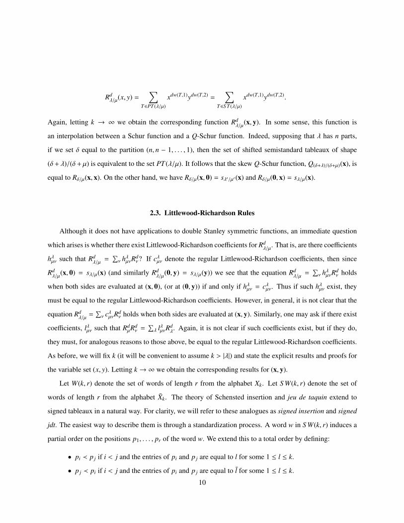
Rdλ/µ(x, y) =

∑T∈PT (λ/µ)

xdw(T,1)ydw(T,2) =∑

T∈S T (λ/µ)

xdw(T,1)ydw(T,2).

Again, letting k → ∞ we obtain the corresponding function Rdλ/µ

(x, y). In some sense, this function is

an interpolation between a Schur function and a Q-Schur function. Indeed, supposing that λ has n parts,

if we set δ equal to the partition (n, n − 1, . . . , 1), then the set of shifted semistandard tableaux of shape

(δ+ λ)/(δ+ µ) is equivalent to the set PT (λ/µ). It follows that the skew Q-Schur function, Q(δ+λ)/(δ+µ)(x), is

equal to Rδ/µ(x, x). On the other hand, we have Rδ/µ(x, 0) = sλ′/µ′(x) and Rδ/µ(0, x) = sλ/µ(x).

2.3. Littlewood-Richardson Rules

Although it does not have applications to double Stanley symmetric functions, an immediate question

which arises is whether there exist Littlewood-Richardson coefficients for Rdλ/µ

. That is, are there coefficients

hλµν such that Rdλ/µ

=∑ν hλµνR

dν? If cλµν denote the regular Littlewood-Richardson coefficients, then since

Rdλ/µ

(x, 0) = sλ/µ(x) (and similarly Rdλ/µ

(0, y) = sλ/µ(y)) we see that the equation Rdλ/µ

=∑ν hλµνR

dν holds

when both sides are evaluated at (x, 0), (or at (0, y)) if and only if hλµν = cλµν. Thus if such hλµν exist, they

must be equal to the regular Littlewood-Richardson coefficients. However, in general, it is not clear that the

equation Rdλ/µ

=∑ν cλµνR

dν holds when both sides are evaluated at (x, y). Similarly, one may ask if there exist

coefficients, lλµν such that RdµRd

ν =∑λ lλµνR

dλ. Again, it is not clear if such coefficients exist, but if they do,

they must, for analogous reasons to those above, be equal to the regular Littlewood-Richardson coefficients.

As before, we will fix k (it will be convenient to assume k > |λ|) and state the explicit results and proofs for

the variable set (x, y). Letting k → ∞ we obtain the corresponding results for (x, y).

Let W(k, r) denote the set of words of length r from the alphabet Xk. Let S W(k, r) denote the set of

words of length r from the alphabet Xk. The theory of Schensted insertion and jeu de taquin extend to

signed tableaux in a natural way. For clarity, we will refer to these analogues as signed insertion and signed

jdt. The easiest way to describe them is through a standardization process. A word w in S W(k, r) induces a

partial order on the positions p1, . . . , pr of the word w. We extend this to a total order by defining:

• pi ≺ p j if i < j and the entries of pi and p j are equal to l for some 1 ≤ l ≤ k.

• p j ≺ pi if i < j and the entries of pi and p j are equal to l for some 1 ≤ l ≤ k.

10

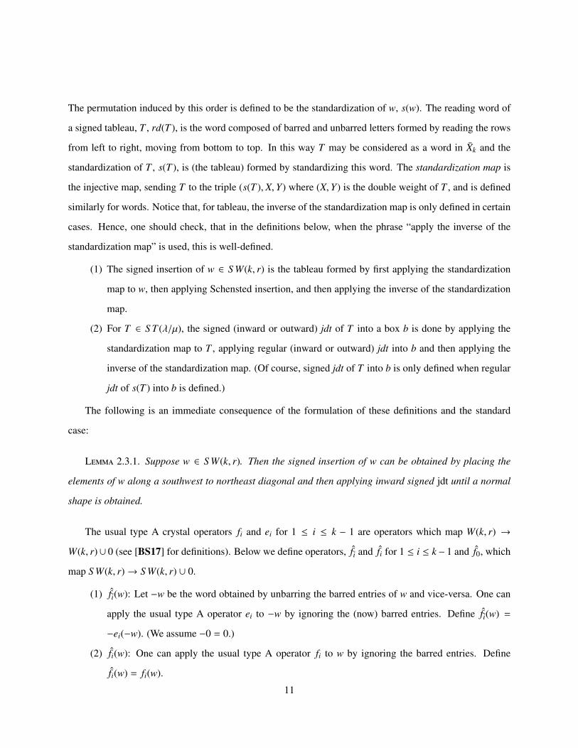
The permutation induced by this order is defined to be the standardization of w, s(w). The reading word of

a signed tableau, T , rd(T ), is the word composed of barred and unbarred letters formed by reading the rows

from left to right, moving from bottom to top. In this way T may be considered as a word in Xk and the

standardization of T , s(T ), is (the tableau) formed by standardizing this word. The standardization map is

the injective map, sending T to the triple (s(T ), X,Y) where (X,Y) is the double weight of T , and is defined

similarly for words. Notice that, for tableau, the inverse of the standardization map is only defined in certain

cases. Hence, one should check, that in the definitions below, when the phrase “apply the inverse of the

standardization map” is used, this is well-defined.

(1) The signed insertion of w ∈ S W(k, r) is the tableau formed by first applying the standardization

map to w, then applying Schensted insertion, and then applying the inverse of the standardization

map.

(2) For T ∈ S T (λ/µ), the signed (inward or outward) jdt of T into a box b is done by applying the

standardization map to T , applying regular (inward or outward) jdt into b and then applying the

inverse of the standardization map. (Of course, signed jdt of T into b is only defined when regular

jdt of s(T ) into b is defined.)

The following is an immediate consequence of the formulation of these definitions and the standard

case:

Lemma 2.3.1. Suppose w ∈ S W(k, r). Then the signed insertion of w can be obtained by placing the

elements of w along a southwest to northeast diagonal and then applying inward signed jdt until a normal

shape is obtained.

The usual type A crystal operators fi and ei for 1 ≤ i ≤ k − 1 are operators which map W(k, r) →

W(k, r)∪ 0 (see [BS17] for definitions). Below we define operators, fi and fi for 1 ≤ i ≤ k− 1 and f0, which

map S W(k, r)→ S W(k, r) ∪ 0.

(1) fi(w): Let −w be the word obtained by unbarring the barred entries of w and vice-versa. One can

apply the usual type A operator ei to −w by ignoring the (now) barred entries. Define fi(w) =

−ei(−w). (We assume −0 = 0.)

(2) fi(w): One can apply the usual type A operator fi to w by ignoring the barred entries. Define

fi(w) = fi(w).

11

(3) f0(w): Among all entries which are 1 or 1, consider the leftmost one. If this entry is 1 change it to

1. Otherwise, f0(w) = 0.

We have

• f1(21212) = 21112

• f0(21212) = 21212

• f1(21212) = 21222

• f1(22111) = 0

• f0(22111) = 0

• f1(22111) = 0

We define the operators ei, ei, and e0 to be the respective inverses of fi, fi, and f0. If all of the operators

ei, ei, and e0 are 0 for w, we say that w is highest weight. Similarly, if all of the operators fi, fi, and f0 are 0

for w, we say that w is lowest weight.

Suppose w ∈ S W(k, r) for some r < k, then w is lowest weight if and only if:

• w has no barred entries.

• Reading w from left to right one has that all times one has read no more is than i + 1s for each

1 ≤ i ≤ k − 1.

and similarly, w is highest weight if and only if:

• w has only barred entries.

• Reading w from left to right one has that all times one has read no more is than ¯i + 1s for each

1 ≤ i ≤ k − 1.

The operators fi, fi, and f0 (and their inverses) are defined on signed tableaux by letting them act on the

reading word (the operators fi are defined on semistandard tableau in the same way). We note here that, on

a signed tableau, T , fi has the following alternative description:

• fi(T ): Transpose T . Then change each i to −i and add k + 1 to all entries. Then apply the usual

type A operator f−i+k. Then subtract k + 1 from all entries, change each −i to i, and transpose.

It is clear from the descriptions above that for any normal shape signed tableau, there is a unique highest

and lowest weight (Recall that we assume k > |λ|). Moreover, this fact along with the fact the signed

12

insertion commutes with our operators (see below) means that for any connected component of the crystal

on signed words has a unique highest and lowest weight.

Below, we include the entire crystal structure for k = 2 and λ = (2, 1) using the color conventions:

• f1: −→

• f0: −→

• f1: −→

-2 -1-2

-2 -1-1

-2 -11

-2 -12

-2 12

-1 12

1 12

1 22

-2 1-2

-2 1-1

-1 1-1

-1 11

-1 21

-1 22

-2 2-2

-2 11

-1 2-1

-2 22

-2 2-1

-2 21

Theorem 2.3.2. Let x ∈ {k − 1 · · · 1, 0, 1, k − 1}. Suppose T ′ is obtained from T by performing (reverse

or forward) signed jdt into box b. Then fx(T ′) = 0 if and only if fx(T ) = 0. Otherwise, fx(T ′) is obtained

from fx(T ) by performing (reverse or forward) signed jdt into b.

13

Proof. The result for fi follows from the usual result for fi. The result for fi can be obtained similarly

using the alternative description of fi. For f0 note that the leftmost lowest 1 or 1 is preserved under signed

jdt moves and that the whether the leftmost lowest 1 or 1 is a 1 or a 1 does not affect the structure of signed

jdt at all. �

By lemma 2.3.1 we have:

Corollary 2.3.3. Let x ∈ {k − 1 · · · 1, 0, 1, k−1}. Suppose T is obtained from w by performing signed in-

sertion. Then fx(T ) = 0 if and only if fx(w) = 0, and otherwise, fx(T ), is obtained from fx(w) by performing

signed insertion.

Corollary 2.3.4.

Rdλ/µ(x, y) =

∑ν

cλµνRdν(x, y)(2.1)

Rdµ(x, y)Rd

ν(x, y) =∑λ

cλµνRdλ(x, y)(2.2)

Proof. First we establish 2.1. By theorem 2.3.2, the coefficient of Rdν(x, y) in Rd

λ/µ(x, y) is the number of

lowest weight S T of shape λ/µ that rectify under signed jdt to shape ν. But lowest weight S T of shape λ/µ

are exactly the lowest weight SSYT of shape λ/µ in the alphabet Xk. Moreover, semistandard jdt coincides

with signed jdt for such tableaux. Thus, the coefficient of Rdν(x, y) in Rd

λ/µ(x, y) is also the number of lowest

weight S S YT of shape λ/µ that rectify under semistandard jdt to shape ν, which is cλµν.

To prove 2.2, we need the notion of a tensor product for our operators. Given two signed tableaux, say

S and T , the operators fi, fi, f0 act on S ⊗ T by acting on the word obtained by concatenating the reading

word of T onto the right end of the reading word of S . It follows from corollary 2.3.3, that the coefficient

of Rdλ(x, y) in Rd

µ(x, y)Rdν(x, y) is the number of pairs of (S ,T ) with shapes µ and ν respectively such that the

tensor product S ⊗T is lowest weight with double weight equal to ((0, . . . , 0), (0, . . . , λn, . . . , λ1)). But S ⊗T

is lowest weight under the operators fi, fi, f0 if and only if S and T are SSYT and the tensor product S ⊗ T

is lowest weight under the type A operators, { fi}. Thus the coefficient of Rdλ(x, y) in Rd

µ(x, y)Rdν(x, y) is also

the number of pairs of SSYT, (S ,T ) with shapes µ and ν respectively such that the type A tensor product of

14

SSYT’s, S ⊗ T , is lowest weight, with weight equal to (0, . . . , λn, . . . , λ2, λ1), which is cλµν.

�

2.4. Double Stanley Symmetric Functions

The main purpose of this section is to show that the function:

Fdω(x, y) =

∑v∈RS IF(ω)

xdw(v,1)ydw(v,2),

is symmetric in x and symmetric in y. That is, for any composition β, the coefficient of yβ is a symmetric

function in x and the coefficient of xβ is a symmetric function in y. Moreover, these coefficients are not only

symmetric, but Schur positive.

Let ω ∈ S n. We use Edelman-Greene insertion, [EG87], to create a bijection between RS IF(ω) and

pairs of tableaux, (P,Q), where P is an Edelman-Greene tableau for ω, and Q is a primed tableau of the

same shape. This bijection is described below. Again let us fix k < ∞ for the discussion:

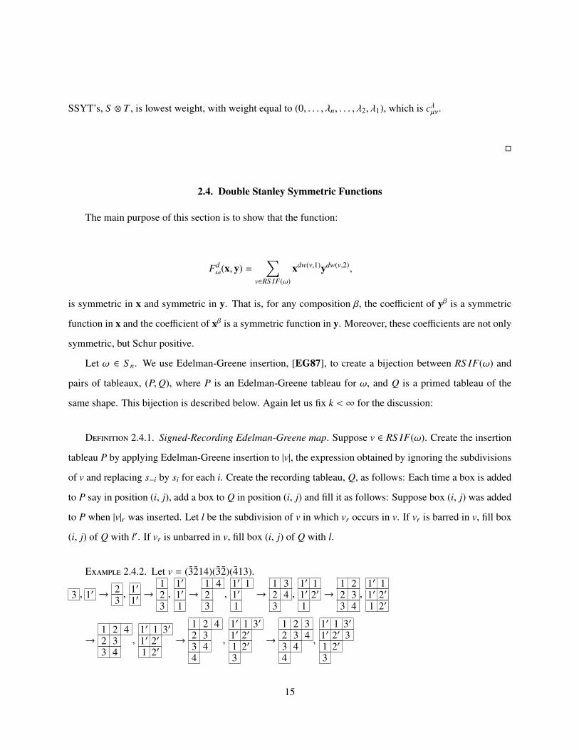
Definition 2.4.1. Signed-Recording Edelman-Greene map. Suppose v ∈ RS IF(ω). Create the insertion

tableau P by applying Edelman-Greene insertion to |v|, the expression obtained by ignoring the subdivisions

of v and replacing s−i by si for each i. Create the recording tableau, Q, as follows: Each time a box is added

to P say in position (i, j), add a box to Q in position (i, j) and fill it as follows: Suppose box (i, j) was added

to P when |v|r was inserted. Let l be the subdivision of v in which vr occurs in v. If vr is barred in v, fill box

(i, j) of Q with l′. If vr is unbarred in v, fill box (i, j) of Q with l.

Example 2.4.2. Let v = (3214)(32)(413).

3 , 1′ → 23, 1′

1′→

123,

1′1′1→

1 423

,1′ 11′1

→1 32 43

,1′ 11′ 2′1

→1 22 33 4

,1′ 11′ 2′1 2′

→1 2 42 33 4

,1′ 1 3′1′ 2′1 2′

→

1 2 42 33 44

,

1′ 1 3′1′ 2′1 2′3

→

1 2 32 3 43 44

,

1′ 1 3′1′ 2′ 31 2′3

15

Theorem 2.4.3. The Signed-Recording Edelman-Greene map is a double weight preserving bijection:

RS IF(ω) ⇒ (P,Q), where P is an Edelman-Greene tableau for ω, and Q is a primed tableau of the same

shape. (The double weight of (P,Q) refers to the double weight of Q.)

Proof. The proof relies on a basic fact of Edelman-Greene insertion of an unsigned reduced word v: If

v = v1 . . . vs is inserted under Edelman-Greene, then vr < vr+1 if and only if the box added to the insertion

tableau in the rth step is in a row weakly above the row where a box is added in the (r + 1)st step. To see the

map is well-defined: Certainly P is an Edelman-Greene tableau. Certainly Q has weakly increasing rows

and columns. There is at most one unbarred i in each column for each i because of the forward direction

of the basic fact. There is at most one barred i in each row for each i because of the backwards direction

of the basic fact. The inverse is obtained by applying reverse Edelman-Greene insertion to P in the order

prescribed by the standardization of Q 3. Subdivisions and the signs of the indices are then added in the

unique way such the resulting factorization has the same double weight as Q. Again, the basic fact implies

that this inverse is well-defined.

�

Combining Theorem 4.3.1 and Corollary 2.2.11 and letting k → ∞ we get the Schur expansion we

desire:

Theorem 2.4.4. For any composition β, the coefficient of yβ in Fdω(x, y) is given by:

p(yβ, ω) =∑

T∈E(ω)

∑µ⊆λ(T )

Kλ(T )µβ sµ′(x).

Here E(ω) is the set of Edelman-Greene tableau for ω, λ(T ) is the shape of T , and Kλµβ is the number of skew

SSYT of shape λ/µ and weight β. Moreover, the coefficient of xβ in Fdω(x, y) is given by p(xβ, ω) = p(yβ, ω−1).

Proof. By theorem 4.3.1 we have

Fdω(x, y) =

∑T∈E(ω)

Rdλ(T )(x, y),

3The reading word and standardization of a primed tableau are defined exactly as for signed tableau. Simply replace the word“barred” with “primed” everywhere it appears in these definitions.

16

and by Corollary 2.2.11 we can express Rdλ(T )(x, y), in terms of signed tableaux. In particular, the coefficient

of yβ in Rdλ(x, y) is equal to:

∑µ⊆λ

Kλµβ

∑S∈S T−(µ)

xdw(S ,1),

where S T−(µ) is the set of signed tableaux of shape µ with only barred entries. Such tableaux are clearly in

weight preserving bijection with the set of SSYT of shape µ′, and so the sum on the right side above may

be replaced by sµ′ . The second statement follows from the fact that Fdω(x, y) = Fd

ω−1(y, x) as can easily be

verified from the definition. �

2.5. Signed-insertion

Our current goal is to construct the obvious analog to the Signed-Recording Edelman-Greene map, i.e.,

the Signed-Insertion Edelman-Greene map, by defining a notion of signed Edelman-Greene insertion, and

creating the recording tableau in the normal way.

A tableau-word, R is a pair (R1,R2) where R1 (the tableau part) is a stack of left-justified rows whose

entries come from the alphabet X and R2 (the word part) is any word using the letters from X . The reading

word of R, rd(R) is the word obtained by reading the rows of R1 from left to right, moving from bottom to

top, and then by reading R2. R is a tableau-word for ω if its reading word is a reduced signed word for ω.

Let K be the map [m − 2] × S m → S m such that K(i, σ1 · · ·σn) = σ1 · · ·σi−2xyzσi+2 · · ·σn where xyz

is the unique three letter sequence which is distinct from, but Knuth equivalent to, σi−1σiσi+1, if such a

sequence exists, and equal to σi−1σiσi+1 otherwise.

Let RS (ω) denote the set of reduced signed words for ω and suppose l(ω) = m. Suppose there exists

some maps K : [m − 2 × RS (ω) → RS (ω), and S: RS (ω) → S m, with the following properties: Supposing

w = w1 · · ·wm ∈ RS (ω) and 2 ≤ i ≤ m − 1:

• S(K(i,w)) = K(i,S(w))

• K(i, (i,w)) = w.

• Setting S(w) = σ1 · · ·σm, we have w j < w j+1 ⇐⇒ σ j < σ j+1, ∀ j < m.

BothK andS can be defined on tableau-words by acting on the reading word, and it follows thatS(K(i,R)) =

K(i,S(R)) for a tableau-word R. A tableau-word, R, whose word part is empty and whose tableau part has

the shape of a partition is called a signed tableau for ω. If in addition, its standardization, S(R), is a standard

17

Young tableau, it is called a signed Edelman-Greene tableau, S EG. We define a functional descent of a

tableau-word to be a descent in its standardization.

We now define an insertion algorithm I which maps RS (ω)→ S EG(ω).

• The map I is defined by starting with the tableau-word (∅,w) and applying the map I′ a total of

l(w) times.

• The map I′ is defined on any tableau-word (R1,R2) by first removing the first entry of R2 and

appending it to the first row of R1 and then applying the map I′′ as many times as possible.

• The map I′′ can be applied to any tableau-word (R1,R2) that has exactly one row, r, that has a

functional descent, and where that functional descent is the second to last entry in r. It is defined

by applying the map I′′′ as many times as possible, and then removing the first entry of r and

appending it to the right end of row r + 1.

• The map I′′′ can be applied to any tableau-word (R1,R2) which has exactly one row, r, that has

a functional descent, and where that functional descent is not the first entry of r. Supposing the

first entry of r is the ath entry in the reading word order, and the last entry of r is the bth entry in

the reading word order, then the map I′′′ applied to R is equal to K(a + 1(· · · (K(b − 2,K(b −

1,R))) · · · )).

One should check, that in the definition above, if K is replaced with K and we assume w has no barred or

repeated entries, we recover the definition of RSK insertion.

Definition 2.5.1. Signed-Insertion Edelman-Greene map: Given v ∈ RS IF(ω), form v by ignoring the

subdivisions of v, so v ∈ RS (ω). We will build up a pair of tableaux, (P,Q) = ((P, ∅),Q), where P is a S EG

and Q is an SSYT of the same shape, starting from ((∅, v), ∅), by successively applying the map I′ to the

lefthand factor l(w) times. Meanwhile we create the recording tableau, Q, simultaneously: Each time a box

is added to the tableau part of lefthand factor add a box in the corresponding position in the righthand factor.

If this occurs during the tth application of I′ and vt is in the sth subdivision of v, then fill this box with s.

Theorem 2.5.2. Suppose that there exists some maps K and S satisfying the conditions mentioned.

Then, for any element ω ∈ Cn, the signed-insertion Edelman-Greene map is a weight-preserving bijection

between RS IF(ω) and pairs (P,Q), where P ∈ S EG(ω) and Q is a semistandard Young tableau of the same

shape as P. (The weight of (P,Q), is taken to be the weight of Q.) In particular, we have:

18

FCω(x) =

∑λ

Eλωsλ(x)

where Eλω is the number of signed Edelman Greene tableaux for ω that have shape λ.

Proof. Let v ∈ RS IF(ω), and suppose v maps to (P,Q). First we show P ∈ S EG(ω). Let I be defined

just as I, except that K is used in place of K . It is easy to verify that I is really just RSK insertion, and so

the tableau I(S(v)) is automatically a standard Young tableau. But since K is assumed to commute with S,

one can check that the standardization of P is the same as I(S(v)), and hence a standard Young tableau. By

definition, this makes a P an S EG.

Suppose Q is not a semistandard Young tableau. The only way this could happen would be if for some

i such that vi and vi+1 are in the same subdivision, the box added at the (i + 1)st step is below the box added

at the ith step. Now, by definition vi < vi+1, and hence by assumption σi < σi+1 where σ = S((∅, ω)).

By commutivity of K and S, boxes are added to Q in the same order as in the recording tableau of RSK

insertion of σ. But it is a standard fact of RSK insertion that σi < σi+1 implies the box added at the (i + 1)st

step is weakly above the box added at the ith step.

Now we show the map is invertible. By similar logic as above, one may verify that if v inserts to (P,Q),

then the order that the boxes are added to Q is the standardization of Q (using the regular definition of

standardization of an SSYT. Thus, we may uniquely reverse the map I (this is possible because the map K

can be inverted for fixed i, i.e., K(i, (i,w)) = w), to get an element of RS (ω) that inserts to P. By adding

subdivisions to this element as dictated by the weight of Q, we find an element that maps under signed-

insertion Edelman-Greene map to (P,Q). The fact that this element is truly in RS IF(ω) (particularly that

the subdivisions are increasing) follows from the converse of the statement in the paragraph above, namely,

if the box added at the (i + 1)st step is weakly above the box added at the ith step then vi < vi+1.

�

In order to make the statement in Theorem 2.5.2 explicit we must construct maps K and S with the

required properties. In particular, this defines explicitly what a S EG tableau is, and how to compute the

coefficients Eλω. We begin by doing this explicitly for a special subset of very simple elements of the Coxeter

group Cn.

19

Definition 2.5.3. We say an element ω ∈ Cn is untangled if the following hold for some (equivalently

all) reduced word w for ω.

(1) s2 does not appear in w

(2) For i > 2, if si and si+1 appear in w, and one of si or si+1 appears more than once, then si−1 and

si+2 do not appear in w.

For instance, the following are untangled: 1010434, 010434676, 10134587.

Theorem 2.5.4. Suppose ω ∈ Cn is untangled4. Then writing

FCω(x) =

∑λ

Eλωsλ(x)

Eλω is the number of tableaux, T , of shape λ composed of entries from the alphabet X such that:

(1) rd(T ) is a reduced signed word for ω.

(2) The rows and columns of T are weakly increasing.

(3) Whenever Ti j = T(i+1) j and Ti j , 0, there exists k > j such that |Tik| = |Ti j| + 1 or there exists l < j

such that |T(i+1)l| = |Ti j| + 1, or else we have both Ti j = 1 = T(i+1) j and Ti( j+1) = 0 = T(i+1)( j+1).

Proof. We explicitly define the maps K and S for ω ∈ Cn untangled. First, we define S, by creating a

total order, ≺, on entries of a signed word w.

(1) If |wi| > 1 or |w j| > 1 then wi ≺ w j if and only if wi < w j in the order X, or wi = w j, and there is

i < k < j such that |wk| = |wi| − 1.

(2) If |wi| ≤ 1 and |w j| ≤ 1, we use the following explicit ordering on the entries of the subword of w

which is composed of 1s, 0s, and 1s, to determine whether wi ≺ w j or w j ≺ wi:

• 01 = 12

• 01 = 21

• 10 = 21

• 10 = 12

• 101 = 213

• 101 = 123

• 101 = 321

• 101 = 231

• 010 = 132

• 010 = 312

• 0101 = 1324

• 0101 = 3124

• 0101 = 2431

• 0101 = 2143

• 1010 = 4231

• 1010 = 4213

• 1010 = 1342

• 1010 = 24134It is likely this theorem holds on a much larger subset of Cn. This will be discussed in the next section

20

Now we define K . Given w = w1 · · ·wn ∈ RS (ω), we define K(i,w) to beW(i + δ,w) where δ is given as

follows. Setting S(w) = σ1 · · ·σn:

(1) If σi−1 < σi < σi+1 or σi+1 < σi < σi−1, then δ = −i.

(2) If σi−1 < σi+1 < σi or σi < σi+1 < σi−1, then δ = 0.

(3) If σi < σi−1 < σi+1 or σi+1 < σi−1 < σi, then δ = 1.

If i = 0, W(i,w) = w. If i > 0, then W(i,w) = w′ = w′1 · · ·w′n, where w′j = w j for all j except where

indicated below. (For a ∈ Z≥0 we consider a and a as elements of X and assume ¯a = a ∈ X, and 0 = 0 ∈ X.)

(1) If ||wi| − |wi+1|| > 1, w′i = wi+1, w′i+1 = wi.

(2) If ||wi| − |wi+1|| = 1, min(|wi|, |wi+1|) > 0 and:

• There exists k < i such that wk = |wi+1|, then w′i = wi+1, w′i+1 = wi, w′k = |wi|.

• There exists k > i + 1 such that wk = ¯|wi|, then w′i = wi+1, w′i+1 = wi, w′k = ¯|wi+1|.

• Otherwise, w′i = wi, w′i+1 = ¯wi+1.

(3) If ||wi| − |wi+1|| = 1, min(|wi|, |wi+1|) = 0 and:

• There is l < i and k > i + 1 such that |wl| ≤ 1 and |wk| ≤ 1. Then w′i = wi+1, w′i+1 = wi,

w′l = wk, w′k = wl.

• There is l < k < i such that |wl| ≤ 1 and |wk| ≤ 1 and:

– wl = 1. Then w′i = wi.

– Otherwise, w′i = wi+1, w′i+1 = wi, w′l = wk, w′k = wl.

• There is i + 1 < l < k such that |wl| ≤ 1 and |wk| ≤ 1 and:

– wk = 1. Then w′i+1 = ¯wi+1.

– Otherwise, w′i = wi+1, w′i+1 = wi, w′l = wk, w′k = wl.

• If none of the cases above occur, then there exists exactly one k < {i, i + 1} such that |wk| ≤ 1.

In this case, w′i = wi, w′i+1 = ¯wi+1, w′k = wk.

One easily checks that for any ω ∈ Cn untangled with l(ω) = m:

(1) S(K(i,w)) = K(i,S(w)) for any w ∈ RS (ω) and 2 ≤ i ≤ m − 1.

(2) K(i, (i,w)) = w for any w ∈ RS (ω) and 2 ≤ i ≤ m − 1.

(3) If w = w1 · · ·wm ∈ RS (ω), and S(w) = σ1 · · ·σm, then for each 1 ≤ i < m we have wi < wi+1 if

and only if σi < σi+1.

21

Thus by Theorem 2.5.2 Eλω is the number of tableau-words for ω which have empty word part and whose

standardization under S is a standard Young tableau. It is not difficult to check that this is equivalent to the

four properties listed in the theorem. �

Below, we use the maps S and K explicitly defined for untangled words in the proof above, and the in-

sertion map I, corresponding to them, to apply the Signed-Insertion Edelman-Greene map in two examples:

Example 2.5.5. Let v = (13)(40)(31). The pair (P,Q) is obtained as follows:

((∅ : 134031

), ∅

)→

((1 : 34031

), 1

)→

((1 3 : 4031

), 1 1

)→

((-4 31

: 041), 1 1

2

)

→

((-4 01 3

: 31), 1 1

2 2

)→

-4 -3

0 31

: 1

, 1 12 23

→ -4 -3 1

0 31

: ∅

, 1 1 32 23

.Example 2.5.6. Let v = (301)(04)(13). The pair (P,Q) is obtained as follows:

((∅ : 3010413

), ∅

)−→

((-3 : 010413

), 1

)−→

((-3 0 : 10413

), 1 1

)−→

((-3 0 1 : 0413

), 1 1 1

)−→

((-3 0 11

: 403), 1 1 1

2

)−→

((-3 0 1 41

: 03), 1 1 1 2

2

)

−→

-3 -1 0 4

01

: 3

, 1 1 1 223

→ -4 -1 0 3

0 31

: ∅

, 1 1 1 22 33

.For ω ∈ An, the t-Stanley symmetric function:

Ftω(x, t) =

∑v∈RS IF(ω)

xw(v)tht(v),

where ht(v) is the number of barred entries in v and w(v) is the vector whose ith coordinate records the total

number of entries in the ith subdivision of v, is Schur-positive. This can be verified from the equation,

Fdω(x, y) =

∑v∈RS IF(ω)

xdw(v,1), ydw(v,2),

by plugging in y = tx. Moreover, as w and K(i,w) always have the same number of barred entries in the

type An case, we have:

22

Corollary 2.5.7. Suppose ω ∈ An is untangled. Then

Ftω(x) =

∑λ

Eλrω sλ(x)tr

where Eλrω is the number of tableaux, T , composed of entries from the alphabet X with shape λ such that:

(1) rd(T ) is a reduced signed word for ω with r barred entries.

(2) The rows and columns of T are weakly increasing.

(3) Whenever Ti j = T(i+1) j, there exists k > j such that |Tik| = |Ti j| + 1 or there exists l < j such that

|T(i+1)l| = |Ti j| + 1.

For ω ∈ Cn such that no word for ω has more than one s0, the parity of the number of barred entries in

w and K(i,w) is always the same. Hence for such ω, which are also untangled the even Stanley symmetric

function and odd Stanley symmetric function:

Fevenω (x) =

∑v∈RS IF(ω)

[−1ht(v) + 1

2

]xw(v) Fodd

ω (x) = −∑

v∈RS IF(ω)

[−1ht(v) − 1

2

]xw(v)

are Schur-positive, and we have:

Corollary 2.5.8. Suppose ω ∈ Cn is untangled and each word for ω has at most one s0. Then

Fevenω (x) =

∑λ

Eλ+ω sλ(x) Fodd

ω (x) =∑λ

Eλ−ω sλ(x)

where Eλ+ω (resp., Eλ−

ω ) is the number of tableaux, T , composed of entries from the alphabet X with

shape λ such that:

(1) rd(T ) is a reduced signed word for ω with even (odd) number of barred entries.

(2) The rows and columns of T are weakly increasing.

(3) Whenever Ti j = T(i+1) j, there exists k > j such that |Tik| = |Ti j| + 1 or there exists l < j such that

|T(i+1)l| = |Ti j| + 1.

23

2.6. Conjectures

Conjecture 2.6.1. The maps K and S assumed to exist in Theorem 2.5.2 exist for any ω ∈ Cn. More-

over, these maps, and the set S EG(ω) defined with respect to S satisfy the following properties:

(1) Let w ∈ RS (ω). Then if any of |wi−1|, |wi|, |wi+1| > 1, then w and K(i,w) have the same number of

barred entries.

(2) Let w ∈ RS (ω). If there is no more than one 0 in w, then the parity of the number of barred entries

of w and K(i,w) is the same.

(3) Let w ∈ RS (ω) and let w′ = K(i,w), then either w1 · · ·wi−2 = w′1 · · ·w′i−2 or wi+2 · · ·wn =

w′i+2 · · ·w′n as signed words, or both.

(4) S EG(ω) is a subset of the set of signed tableaux for ω with weakly increasing rows and columns.

(5) If T is a signed tableau for ω, then I(rd(T )) = T if and only if T ∈ S EG(ω).

Consider Cn with generators {s0, s1, s2, . . . , sn}. We say ω ∈ Cp−qn if ω ∈ Cn and each reduced word for

ω contains p generators of which q are equal to s0. For instance, Cp−0n is the subset of length p elements in

An.

Definition 2.6.2. We say an element ω ∈ Cn is unknotted if the following hold for all reduced words w

for ω.

(1) If the sequence s0s1s0s1 appears in w, then s2 does not.

(2) For i > 0 if the sequence sisi+1si appears in w then si+2 does not.

For instance 123454, 2101232, 1010343, and 213243 are unknotted. Clearly unknotted is a weaker

condition than untangled. The subset of Cp−qn composed of unknotted elements is denoted ¯Cp−q

n . We con-

clude by establishing the results in 2.5.4, 2.5.7, and 2.5.8 to for ¯Cp−qn for certain n, p, and q as equalities of

polynomials in three variables. In order to do so for 2.5.8 it is first good to know:

Theorem 2.6.3. If ω ∈ C8−18 then Fodd

ω (x1, x2, x3) and Fevenω (x1, x2, x3) are symmetric and Schur positive.

Proof. Computer verification. There are 4489 such ω to check. �

Conjecture 2.6.4. The above holds for all ω ∈ Cp−1n with (x1, x2, x3) replaced by (x).

Proposition 2.6.5. Suppose ω ∈ ¯C8−18 Then

24

Fevenω (x1, x2, x3) =

∑λ

Eλ+ω sλ(x1, x2, x3) Fodd

ω (x1, x2, x3) =∑λ

Eλ−ω sλ(x1, x2, x3)

where Eλ+ω (resp., Eλ−

ω ) is the number of tableaux, T , composed of entries from the alphabet X with

shape λ = (λ1, λ2, λ3) such that:

(1) rd(T ) is a reduced signed word for ω with even (odd) number of barred entries.

(2) The rows and columns of T are weakly increasing.

(3) Whenever Ti j = T(i+1) j, there exists k > j such that |Tik| = |Ti j| + 1 or there exists l < j such that

|T(i+1)l| = |Ti j| + 1.

Proof. Computer verification. There are 2511 such ω to check. �

Conjecture 2.6.6. The above holds for all ω ∈ ¯Cp−1n with (x1, x2, x3) replaced by (x).

Example 2.6.7. For instance, if ω = s1s0s1s2s3s4s3s6 then E(4,3,1)−ω counts the 2 tableaux:

-1 2 3 40 4 61

-6 -4 -3 40 1 21

.

Proposition 2.6.8. If ω ∈ ¯C9−09 . Then

Ftω(x1, x2, x3) =

∑λ

Eλrω sλ(x1, x2, x3)tr

where Eλrω is the number of tableaux, T , composed of entries from the alphabet X with shape λ = (λ1, λ2, λ3)

such that:

(1) rd(T ) is a reduced signed word for ω with r barred entries.

(2) The rows and columns of T are weakly increasing.

(3) Whenever Ti j = T(i+1) j, there exists k > j such that |Tik| = |Ti j| + 1 or there exists l < j such that

|T(i+1)l| = |Ti j| + 1.

Proof. Computer verification. There are 3167 such ω to check. �

Conjecture 2.6.9. The above holds for all ω ∈ ¯Cp−0n with (x1, x2, x3) replaced by x.

25

Example 2.6.10. For instance, if ω = s3s4s8s2s3s5s6s1s5 ∈¯C9−09 then E(3,3,3)1

ω counts the 2 tableaux:

-6 1 32 4 53 6 8

-6 1 52 3 53 4 8

.

Proposition 2.6.11. Suppose ω ∈ ¯C7−q7 for any q. Then

FCω(x1, x2, x3) =

∑λ

Eλωsλ(x1, x2, x3)

where Eλω is the number of tableaux, T , of shape λ = λ1, λ2, λ3 composed of entries from the alphabet X

such that:

(1) rd(T ) is a reduced signed word for ω.

(2) The rows and columns of T are weakly increasing.

(3) Whenever Ti j = T(i+1) j and Ti j , 0, there exists k > j such that |Tik| = |Ti j| + 1 or there exists l < j

such that |T(i+1)l| = |Ti j| + 1, or else we have both Ti j = 1 = T(i+1) j and Ti( j+1) = 0 = T(i+1)( j+1).

Proof. Computer verification. There are 1414 such ω to check. �

Conjecture 2.6.12. The above holds for all ω ∈ ¯Cp−qn with (x1, x2, x3) replaced by x.

Example 2.6.13. For instance, if ω = s1s0s1s2s1s0s1 ∈¯C7−27 then E(4,3,0)

ω = E(4,2,1)ω = E(3,3,1)

ω = E(3,3,2)ω =

1 and all others are 0. The corresponding tableaux are:

-2 -1 0 1-1 0 1

-2 -1 0 10 11

-1 0 10 1 21

-2 0 10 11 2

.

Example 2.6.14. For instance, if ω = s1s0s1s0s3s4s5 ∈¯C7−27 then E(4,3,0)

ω counts the 6 tableaux:

-4 -1 0 5-3 -1 0

-4 0 1 50 1 3

-4 -1 0 5-1 0 3

-5 -1 0 10 3 4

-5 -1 0 1-3 0 4

-1 0 1 50 3 4

.

26

CHAPTER 3

Primed and Signed Tableaux of Shifted Shape: Type C Stanley Symmetric

Functions

This chapter is based on the work in [HPS17].

3.1. Introduction

In this chapter, we carry out a crystal analysis of the Stanley symmetric functions FCw(x) of type C,

indexed by a Coxeter group element w. In particular, we use Kraskiewicz insertion [Kra89, Kra95] and

Haiman’s mixed insertion [Hai89] to find a crystal structure on shifted semistandard tableaux, which in turn

implies a crystal structure Bw on reduced unimodal factorizations (as defined in chapter 1) of w for which

FCw(x) is a character. Moreover, we present a type A crystal isomorphism Φ : Bw →

⊕λB⊕gwλλ for some

combinatorially defined nonnegative integer coefficients gwλ; here Bλ is the type A highest weight crystal of

highest weight λ . This implies the desired decomposition FCw(x) =

∑λ gwλsλ(x) (see Corollary 3.3.10) and

similarly for type B.

Recall the Coxeter group WC of type Cn as defined in chapter 2. It is often convenient to write down an

element of a Coxeter group as a sequence of indices of si in the product representation of the element. For

example, the element w = s2s1s2s1s0s1s0s1 is represented by the word w = 2120101. A word of shortest

length ` is referred to as a reduced word and `(w) := ` is referred as the length of w.

Recall from chapter 2 that the [BH95, FK96, Lam95] type C Stanley symmetric function associated to

w ∈ WC is defined as

(3.1) FCw(x) =

∑A∈U(w)

2nz(A)xwt(A).

Here x = (x1, x2, x3, . . .) and xv = xv11 xv2

2 xv33 · · · .

In Section 3.2 we describe our crystal isomorphism by combining a slight generalization of the Kraskiewicz

insertion [Kra89, Kra95] and Haiman’s mixed insertion [Hai89]. The main result regarding the crystal

27

structure under Haiman’s mixed insertion is stated in Theorem 3.3.3. The combinatorial interpretation of

the coefficients gwλ is given in Corollary 3.3.10. In Section 3.4, we provide an alternative interpretation of

the coefficients gwλ in terms of semistandard unimodal tableaux. Appendices A.1 and A.2 are reserved for

the proofs of Theorems 3.3.3 and 3.3.6.

3.2. Crystal isomorphism

In this section, we combine a slight generalization of the Kraskiewicz insertion, reviewed in Sec-

tion 3.2.1, and Haiman’s mixed insertion, reviewed in Section 3.2.2, to provide an isomorphism of crystals

between the crystal of words Bh and certain sets of primed tableaux of shifted shape.

3.2.1. Kraskiewicz insertion. In this section, we describe the Kraskiewicz insertion. To do so, we first

need to define the Edelman–Greene insertion [?]. It is defined for a word w = w1 . . .w` and a letter k such

that the concatenation w1 . . .w`k is an A-type reduced word. The Edelman–Greene insertion of a letter k

into an increasing word w = w1 . . .w`, denoted by w f k, is constructed as follows:

(1) If w` < k, then w f k = w′, where w′ = w1w2 . . .w` k.

(2) If k > 0 and k k + 1 = wi wi+1 for some 1 6 i < `, then w f k = k + 1 f w.

(3) Else let wi be the leftmost letter in w such that wi > k. Then w f k = wi f w′, where

w′ = w1 . . .wi−1 k wi+1 . . .w`.

In the cases above, when w f k = k′ f w′, the symbol k′ f w′ indicates a word w′ together with a

“bumped” letter k′.

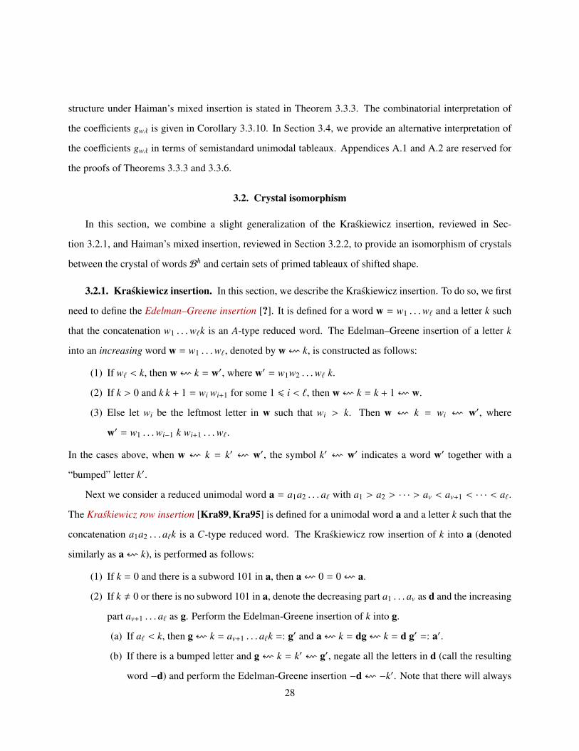
Next we consider a reduced unimodal word a = a1a2 . . . a` with a1 > a2 > · · · > av < av+1 < · · · < a`.

The Kraskiewicz row insertion [Kra89,Kra95] is defined for a unimodal word a and a letter k such that the

concatenation a1a2 . . . a`k is a C-type reduced word. The Kraskiewicz row insertion of k into a (denoted

similarly as a f k), is performed as follows:

(1) If k = 0 and there is a subword 101 in a, then a f 0 = 0 f a.

(2) If k , 0 or there is no subword 101 in a, denote the decreasing part a1 . . . av as d and the increasing

part av+1 . . . a` as g. Perform the Edelman-Greene insertion of k into g.

(a) If a` < k, then g f k = av+1 . . . a`k =: g′ and a f k = dg f k = d g′ =: a′.

(b) If there is a bumped letter and g f k = k′ f g′, negate all the letters in d (call the resulting

word −d) and perform the Edelman-Greene insertion −d f −k′. Note that there will always

28

be a bumped letter, and so −d f −k′ = −k′′f −d′ for some decreasing word d′. The result

of the Kraskiewicz insertion is: a f k = d[g f k] = d[k′ f g′] = −[−d f −k′] g′ =

[k′′f d′]g′ = k′′f a′, where a′ := d′g′.

Example 3.2.1.

31012 f 0 = 0 f 31012, 3012 f 0 = 0 f 3102,

31012 f 1 = 1 f 32012, 31012 f 3 = 310123.

The insertion is constructed to “commute” a unimodal word with a letter: If a f k = k′ f a′, the two

elements of the type C Coxeter group corresponding to concatenated words a k and k′a′ are the same.

The type C Stanley symmetric functions (3.1) are defined in terms of unimodal factorizations. To put

the formula on a completely combinatorial footing, we need to treat the powers of 2 by introducing signed

unimodal factorizations. A signed unimodal factorization of w ∈ WC is a unimodal factorization A of w,

in which every non-empty factor is assigned either a + or − sign. Denote the set of all signed unimodal

factorizations of w by U±(w).

For a signed unimodal factorization A ∈ U±(w), define wt(A) to be the vector with i-th coordinate equal

to the number of letters in the i-th factor of A. Notice from (3.1) that

(3.1) FCw(x) =

∑A∈U±(w)

xwt(A).

We will use the Kraskiewicz insertion to construct a map between signed unimodal factorizations of a

Coxeter group element w and pairs of certain types of tableaux (P,T). We define these types of tableaux

next.

A shifted diagram S(λ) associated to a partition λ with distinct parts is the set of boxes in positions

{(i, j) | 1 6 i 6 `(λ), i 6 j 6 λi + i − 1}. Here, we use English notation, where the box (1, 1) is always

top-left.

Let X◦n be an ordered alphabet of n letters X◦n = {0 < 1 < 2 < · · · < n − 1}, and let X′n be an ordered

alphabet of n letters together with their primed counterparts as X′n = {1′ < 1 < 2′ < 2 < · · · < n′ < n}.

Let λ be a partition with distinct parts. A unimodal tableau P of shape λ on n letters is a filling of S(λ)

with letters from the alphabet X◦n such that the word Pi obtained by reading the ith row from the top of P

from left to right, is a unimodal word, and Pi is the longest unimodal subword in the concatenated word

29

Pi+1Pi [BHRY14] (cf. also with decomposition tableaux [Ser10,Cho13]). The reading word of a unimodal

tableau P is given by πP = P`P`−1 . . . P1. A unimodal tableau is called reduced if πP is a type C reduced

word corresponding to the Coxeter group element wP. Given a fixed Coxeter group element w, denote the

set of reduced unimodal tableaux P of shape λ with wP = w asUT w(λ).

A shifted primed tableau T of shape λ on n letters (cf. semistandard Q-tableau [Lam95]) is a filling of

S(λ) with letters from the alphabet X′n such that:

(1) The entries are weakly increasing along each column and each row of T.

(2) Each row contains at most one i′ for every i = 1, . . . , n.

(3) Each column contains at most one i for every i = 1, . . . , n.

Denote the set of shifted primed tableaux of shape λ by PT ±(λ). Given an element T ∈ PT ±(λ), define

the weight of the tableau wt(T) as the vector with i-th coordinate equal to the total number of letters in T

that are either i or i′.

Example 3.2.2.( 4 3 2 0 1

2 1 20

,1 1 2′ 3′ 3

2′ 2 3′4

)is a pair consisting of a unimodal tableau and a shifted

primed tableau both of shape (5, 3, 1).

For a reduced unimodal tableau P with rows P`, P`−1, . . . , P1, the Kraskiewicz insertion of a letter k into

tableau P (denoted again by P f k) is performed as follows:

(1) Perform Kraskiewicz insertion of the letter k into the unimodal word P1. If there is no bumped

letter and P1 f k = P′1, the algorithm terminates and the new tableau P′ consists of rows

P`, P`−1, . . . , P2, P′1. If there is a bumped letter and P1 f k = k′f P′1, continue the algorithm by

inserting k′ into the unimodal word P2.

(2) Repeat the previous step for the rows of P until either the algorithm terminates, in which case the

new tableau P′ consists of rows P`, . . . , Ps+1, P′s, . . . , P′1, or, the insertion continues until we bump

a letter ke from P`, in which case we then put ke on a new row of the shifted shape of P′, so that

the resulting tableau P′ consists of rows ke, P′`, . . . , P′1.

Example 3.2.3.4 3 2 0 1

2 1 20

f 0 =4 3 2 1 0

2 1 00 1

,

30

since the insertions row by row are given by 43201 f 0 = 0 f 43210, 212 f 0 = 1 f 210, and

0 f 1 = 01.

Lemma 3.2.4. [Kra89] Let P be a reduced unimodal tableau with reading word πP for an element

w ∈ WC . Let k be a letter such that πPk is a reduced word. Then the tableau P′ = P f k is a reduced

unimodal tableau, for which the reading word πP′ is a reduced word for wsk.

Lemma 3.2.5. [Lam95, Lemma 3.17] Let P be a unimodal tableau, and a a unimodal word such that

πPa is reduced. Let (x1, y1), . . . , (xr, yr) be the (ordered) list of boxes added when P f a is computed. Then

there exists an index v, such that x1 < · · · < xv > · · · > xr and y1 > · · · > yv < · · · < yr.

Let A ∈ U±(w) be a signed unimodal factorization with unimodal factors a1, a2, . . . , an. We recur-

sively construct a sequence (∅, ∅) = (P0,T0), (P1,T1), . . . , (Pn,Tn) = (P,T) of tableaux, where Ps ∈

UT (a1a2...as)(λ(s)) and Ts ∈ PT

±(λ(s)) are tableaux of the same shifted shape λ(s).

To obtain the insertion tableau Ps, insert the letters of as one by one from left to right, into Ps−1. Denote

the shifted shape of Ps by λ(s). Enumerate the boxes in the skew shape λ(s)/λ(s−1) in the order they appear

in Ps. Let these boxes be (x1, y1), . . . , (x`s , y`s).

Let v be the index that is guaranteed to exist by Lemma 3.2.5 when we compute Ps−1 f as. The record-

ing tableau Ts is a shifted primed tableau obtained from Ts−1 by adding the boxes (x1, y1), . . . , (xv−1, yv−1),

each filled with the letter s′, and the boxes (xv+1, yv+1), . . . , (x`s , y`s), each filled with the letter s. The special

case is the box (xv, yv), which could contain either s′ or s. The letter is determined by the sign of the factor

as: If the sign is −, the box is filled with the letter s′, and if the sign is +, the box is filled with the letter s.

We call the resulting map the primed Kraskiewicz map KR′.

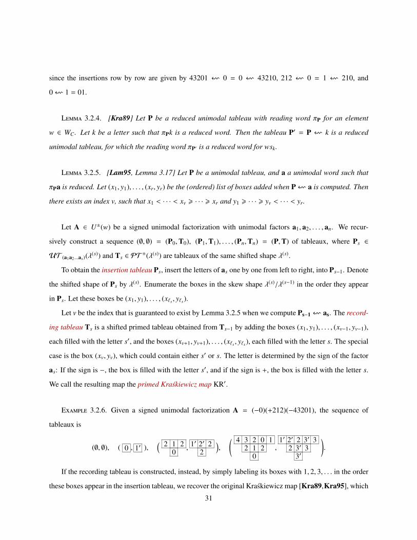
Example 3.2.6. Given a signed unimodal factorization A = (−0)(+212)(−43201), the sequence of

tableaux is

(∅, ∅), ( 0 , 1′ ),( 2 1 2

0, 1′ 2′ 2

2

),

( 4 3 2 0 12 1 2

0,

1′ 2′ 2 3′ 32 3′ 3

3′

).

If the recording tableau is constructed, instead, by simply labeling its boxes with 1, 2, 3, . . . in the order

these boxes appear in the insertion tableau, we recover the original Kraskiewicz map [Kra89,Kra95], which

31

is a bijection

KR: R(w)→⋃λ

[UT w(λ) × ST (λ)

],

where ST (λ) is the set of standard shifted tableau of shape λ, i.e., the set of fillings of S(λ) with letters

1, 2, . . . , |λ| such that each letter appears exactly once, each row filling is increasing, and each column filling

is increasing.

Theorem 3.2.7. The primed Kraskiewicz map is a bijection

KR′ : U±(w)→⋃λ

[UT w(λ) × PT ±(λ)

].

Proof. First we show that the map is well-defined: Let A ∈ U±(w) such that KR′(A) = (P,Q). The fact

that P is a unimodal tableau follows from the fact that KR is well-defined. On the other hand, Q satisfies

Condition (1) in the definition of shifted primed tableaux since its entries are weakly increasing with respect

to the order the associated boxes are added to P. Now fix an s and consider the insertion Ps−1 f as. Refer to

the set-up in Lemma 3.2.5. Then, y1 < · · · < yv implies there is at most one s′ in each row and yv > · · · > y`s

implies there is at most one s in each column, so Conditions (2) and (3) of the definition have been verified,

implying that indeed Q is a shifted primed tableau.

Now suppose (P,Q) ∈⋃λ

[UT w(λ)×PT ±(λ)

]. The ordering of the alphabet X′ induces a partial order

on the set of boxes of Q. Refine this ordering as follows: Among boxes containing an s′, box b is greater

than box c if box b lies below box c. Among boxes containing an s, box b is greater than box c if box b lies

to the right of box c. Let the standard shifted tableau induced by the resulting total order be denoted Q∗.

Let w = KR−1(P,Q∗). Divide w into factors, where the size of the s-th factor is equal to the s-th entry

in wt(Q). Let A = a1 . . . an be the resulting factorization, where the sign of as is determined as follows:

Consider the lowest leftmost box in Q that contains an s or s′ (such a box must exist if as , ∅). If this

box contains an s give as a positive sign, and otherwise a negative sign. Let b1, . . . , b|as | denote the boxes of

Q∗ corresponding to as under KR−1. The construction of Q∗ and the fact that Q is a shifted primed tableau

imply that the coordinates of these boxes satisfy the hypothesis of Lemma 3.2.5. Since these are exactly the

boxes that appear when we compute Ps−1 f as, Lemma 3.2.5 implies that as is unimodal. It follows that A

is a signed unimodal factorization mapping to (P,Q) under KR′. It is not hard to see A is unique. �

32

Theorem 3.2.7 and Equation (3.1) imply the following relation:

(3.2) FCw(x) =

∑λ

∣∣∣UT w(λ)∣∣∣ ∑

T∈PT ±(λ)

xwt(T).

Remark 3.2.8. The sum∑

T∈PT ±(λ) xwt(T) is also known as the Q-Schur function. The expansion (3.2),

with a slightly different interpretation of Q-Schur function, was shown in [BH95].

At this point, we are halfway there to expand FCw(x) in terms of Schur functions. In the next section we

introduce a crystal structure on the set PT (λ) of shifted semistandard tableaux.

3.2.2. Mixed insertion. SetBh = Bh∞. Similar to the well-known RSK-algorithm, mixed insertion [Hai89]

gives a bijection between Bh and the set of pairs of tableaux (T,Q), but in this case T is shifted primed

tableau of shape λ and Q is a standard shifted tableau of the same shape.

An (shifted primed tableau of shape λ (cf. semistandard P-tableau [Lam95] or semistandard marked

shifted tableau [Cho13]) is a shifted primed tableau T of shape λ with only unprimed elements on the main

diagonal. Denote the set of shifted primed tableaux of shape λ by PT (λ). The weight function wt(T) of

T ∈ PT (λ) is inherited from the weight function of shifted primed tableaux, that is, it is the vector with i-th

coordinate equal to the number of letters i′ and i in T. We can simplify (3.2) as

(3.3) FCw(x) =

∑λ

2`(λ)∣∣∣UT w(λ)

∣∣∣ ∑T∈PT (λ)

xwt(T).

Remark 3.2.9. The sum∑

T∈PT (λ) xwt(T) is also known as a P-Schur function.

Given a word b1b2 . . . bh in the alphabet X = {1 < 2 < 3 < · · · }, we recursively construct a sequence

of tableaux (∅, ∅) = (T0,Q0), (T1,Q1), . . . , (Th,Qh) = (T,Q), where Ts ∈ PT (λ(s)) and Qs ∈ ST (λ(s)).

To obtain the tableau Ts, insert the letter bs into Ts−1 as follows. First, insert bs into the first row of Ts−1,

bumping out the leftmost element y that is strictly greater than bi in the alphabet X′ = {1′ < 1 < 2′ < 2 <

· · · }.

(1) If y is not on the main diagonal and y is not primed, then insert it into the next row, bumping out

the leftmost element that is strictly greater than y from that row.

(2) If y is not on the main diagonal and y is primed, then insert it into the next column to the right,

bumping out the topmost element that is strictly greater than y from that column.

33

(3) If y is on the main diagonal, then it must be unprimed. Prime y and insert it into the column on the

right, bumping out the topmost element that is strictly greater than y from that column.

If a bumped element exists, treat it as a new y and repeat the steps above – if the new y is unprimed, row-

insert it into the row below its original cell, and if the new y is primed, column-insert it into the column to

the right of its original cell.

The insertion process terminates either by placing a letter at the end of a row, bumping no new element,

or forming a new row with the last bumped element.

Example 3.2.10. Under mixed insertion,

2 2 3′ 33 3

← 1 =1 2′ 3′ 3

2 3′3

.

Let us explain each step in detail. The letter 1 is inserted into the first row bumping out the 2 from the main

diagonal, making it a 2′, which is then inserted into the second column. The letter 2′ bumps out 2, which

we insert into the second row. Then 3 from the main diagonal is bumped from the second row, making it a

3′, which is then inserted into third column. The letter 3′ bumps out the 3 on the second row, which is then

inserted as the first element in the third row.

The shapes of Ts−1 and Ts differ by one box. Add that box to Qs−1 with a letter s in it, to obtain the

standard shifted tableau Qs.

Example 3.2.11. For a word 332332123, some of the tableaux in the sequence (Ti,Qi) are

( 2 3′3, 1 2

3

),

( 2 2 3′ 33 3

, 1 2 4 53 6

),

( 1 2′ 2 3′ 32 3′ 3

3,

1 2 4 5 93 6 8

7

).

Theorem 3.2.12. [Hai89] The construction above gives a bijection

HM: Bh →⋃λ`h

[PT (λ) × ST (λ)

].

The bijection HM is called a mixed insertion. If HM(b) = (T,Q), denote PHM(b) = T and RHM(b) = Q.

34

3.3. Explicit crystal operators on shifted primed tableaux

We consider the alphabet X′ = {1′ < 1 < 2′ < 2 < 3′ < · · · } of primed and unprimed letters. It is useful

to think about the letter (i + 1)′ as a number i + 0.5. Thus, we say that letters i and (i + 1)′ differ by half a

unit and letters i and (i + 1) differ by a whole unit.

Given a shifted primed tableau T, we construct the reading word rw(T) as follows:

(1) List all primed letters in the tableau, column by column, from top to bottom within each column,

moving from the rightmost column to the left, and with all the primes removed (i.e. all letters are

increased by half a unit). (Call this part of the word the primed reading word.)

(2) Then list all unprimed elements, row by row, left to right within each row, moving from the bot-

tommost row to the top. (Call this part of the word the unprimed reading word.)

To find the letter on which the crystal operator fi acts, apply the bracketing rule for letters i and i + 1

within the reading word rw(T). If all letters i are bracketed in rw(T), then fi(T) = 0. Otherwise, the

rightmost unbracketed letter i in rw(T) corresponds to an i or an i′ in T, which we call bold unprimed i or

bold primed i respectively.

If the bold letter i is unprimed, denote the cell it is located in as x.

If the bold letter i is primed, we conjugate the tableau T first.

The conjugate of a shifted primed tableau T is obtained by reflecting the tableau over the main diagonal,

changing all primed entries k′ to k and changing all unprimed elements k to (k + 1)′ (i.e. increase the entries

of all boxes by half a unit). The main diagonal is now the North-East boundary of the tableau. Denote the

resulting tableau as T∗.

Under the transformation T → T∗, the bold primed i is transformed into bold unprimed i. Denote the

cell it is located in as x.

Given any cell z in a shifted primed tableau T (or conjugated tableau T∗), denote by c(z) the entry con-

tained in cell z. Denote by zE the cell to the right of z, zW the cell to its left, zS the cell below, and zN the cell

above. Denote by z∗ the corresponding conjugated cell in T∗ (or in T). Now, consider the box xE (in T or in

T∗) and notice that c(xE) > (i + 1)′.

Crystal operator fi on shifted primed tableaux:

35

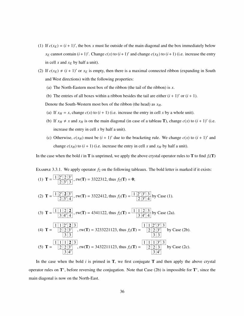
(1) If c(xE) = (i + 1)′, the box x must lie outside of the main diagonal and the box immediately below

xE cannot contain (i + 1)′. Change c(x) to (i + 1)′ and change c(xE) to (i + 1) (i.e. increase the entry

in cell x and xE by half a unit).

(2) If c(xE) , (i + 1)′ or xE is empty, then there is a maximal connected ribbon (expanding in South

and West directions) with the following properties:

(a) The North-Eastern most box of the ribbon (the tail of the ribbon) is x.

(b) The entries of all boxes within a ribbon besides the tail are either (i + 1)′ or (i + 1).

Denote the South-Western most box of the ribbon (the head) as xH .

(a) If xH = x, change c(x) to (i + 1) (i.e. increase the entry in cell x by a whole unit).

(b) If xH , x and xH is on the main diagonal (in case of a tableau T), change c(x) to (i + 1)′ (i.e.

increase the entry in cell x by half a unit).

(c) Otherwise, c(xH) must be (i + 1)′ due to the bracketing rule. We change c(x) to (i + 1)′ and

change c(xH) to (i + 1) (i.e. increase the entry in cell x and xH by half a unit).

In the case when the bold i in T is unprimed, we apply the above crystal operator rules to T to find fi(T)

Example 3.3.1. We apply operator f2 on the following tableaux. The bold letter is marked if it exists:

(1) T =1 2′ 2 3′

2 3′ 3, rw(T) = 3322312, thus f2(T) = 0;

(2) T =1 2′ 2 3′

2 3′ 4, rw(T) = 3322412, thus f2(T) =

1 2′ 3′ 32 3′ 4

by Case (1).

(3) T =1 1 2 2

3 4′ 4, rw(T) = 4341122, thus f2(T) =

1 1 2 33 4′ 4

by Case (2a).

(4) T =1 1 2′ 2 3

2 2 3′3 3

, rw(T) = 3233221123, thus f2(T) =1 1 2′ 3′ 3

2 2 3′3 3

by Case (2b).

(5) T =1 1 1 2 3

2 2 3′3 4′

, rw(T) = 3432211123, thus f2(T) =1 1 1 3′ 3

2 2 33 4′

by Case (2c).

In the case when the bold i is primed in T, we first conjugate T and then apply the above crystal

operator rules on T∗, before reversing the conjugation. Note that Case (2b) is impossible for T∗, since the

main diagonal is now on the North-East.

36

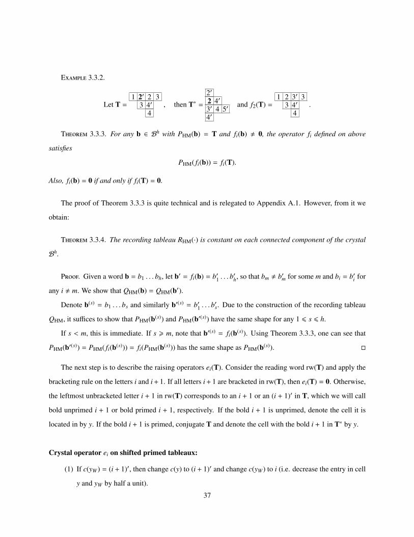
Example 3.3.2.

Let T =1 2′ 2 3

3 4′4

, then T∗ =

2′2 4′3′ 4 5′4′

and f2(T) =1 2 3′ 3

3 4′4

.

Theorem 3.3.3. For any b ∈ Bh with PHM(b) = T and fi(b) , 0, the operator fi defined on above

satisfies

PHM( fi(b)) = fi(T).

Also, fi(b) = 0 if and only if fi(T) = 0.

The proof of Theorem 3.3.3 is quite technical and is relegated to Appendix A.1. However, from it we

obtain:

Theorem 3.3.4. The recording tableau RHM(·) is constant on each connected component of the crystal

Bh.

Proof. Given a word b = b1 . . . bh, let b′ = fi(b) = b′1 . . . b′h, so that bm , b′m for some m and bi = b′i for

any i , m. We show that QHM(b) = QHM(b′).

Denote b(s) = b1 . . . bs and similarly b′(s) = b′1 . . . b′s. Due to the construction of the recording tableau

QHM, it suffices to show that PHM(b(s)) and PHM(b′(s)) have the same shape for any 1 6 s 6 h.

If s < m, this is immediate. If s > m, note that b′(s) = fi(b(s)). Using Theorem 3.3.3, one can see that

PHM(b′(s)) = PHM( fi(b(s))) = fi(PHM(b(s))) has the same shape as PHM(b(s)). �

The next step is to describe the raising operators ei(T). Consider the reading word rw(T) and apply the

bracketing rule on the letters i and i + 1. If all letters i + 1 are bracketed in rw(T), then ei(T) = 0. Otherwise,

the leftmost unbracketed letter i + 1 in rw(T) corresponds to an i + 1 or an (i + 1)′ in T, which we will call

bold unprimed i + 1 or bold primed i + 1, respectively. If the bold i + 1 is unprimed, denote the cell it is

located in by y. If the bold i + 1 is primed, conjugate T and denote the cell with the bold i + 1 in T∗ by y.

Crystal operator ei on shifted primed tableaux:

(1) If c(yW) = (i + 1)′, then change c(y) to (i + 1)′ and change c(yW) to i (i.e. decrease the entry in cell

y and yW by half a unit).

37

(2) If c(yW) < (i + 1)′ or yW is empty, then there is a maximal connected ribbon (expanding in North

and East directions) with the following properties:

(a) The South-Western most box of the ribbon (the head of the ribbon) is y.

(b) The entry in all boxes within a ribbon besides the tail is either i or (i + 1)′.

Denote the North-Eastern most box of the ribbon (the tail) as yT .

(a) If yT = y, change c(y) to i (i.e. decrease the entry in cell y by a whole unit).

(b) If yT , y and yT is on the main diagonal (in case of a conjugate tableau T∗), then change c(y)

to (i + 1)′ (i.e. decrease the entry in cell y by half a unit).

(c) If yT , y and yT is not on the diagonal, the entry of cell yT must be (i + 1)′ and we change c(y)

to (i + 1)′ and change c(yT ) to i (i.e. decrease the entry of cell y and yT by half a unit).

When the bold i + 1 is unprimed, ei(T) is obtained by applying the rules above to T. When the bold i + 1

is primed, we first conjugate T, then apply the raising crystal operator rules on T∗, and then reverse the

conjugation.

Proposition 3.3.5.

ei(b) = 0 if and only if ei(T) = 0.

Proof. According to Lemma A.1.1, the number of unbracketed letters i in b is equal to the number of

unbracketed letters i in rw(T). Since the total number of both letters i and j = i + 1 is the same in b and in

rw(T), that also means that the number of unbracketed letters j in b is equal to the number of unbracketed

letters j in rw(T). Thus, there are no unbracketed letters j in b if and only if there are no unbracketed letters

j in T. �

Theorem 3.3.6. Given a shifted primed tableau T with fi(T) , 0, for the operators ei defined above we

have the following relation:

ei( fi(T)) = T.

The proof of Theorem 3.3.6 is relegated to Appendix A.2.

Corollary 3.3.7. For any b ∈ Bh with HM(b) = (T,Q), the operator ei defined above satisfies

HM(ei(b)) = (ei(T),Q),

38

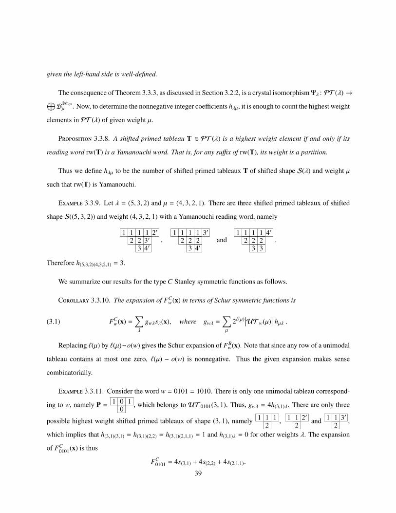
given the left-hand side is well-defined.

The consequence of Theorem 3.3.3, as discussed in Section 3.2.2, is a crystal isomorphism Ψλ : PT (λ)→⊕B⊕hλµµ . Now, to determine the nonnegative integer coefficients hλµ, it is enough to count the highest weight

elements in PT (λ) of given weight µ.

Proposition 3.3.8. A shifted primed tableau T ∈ PT (λ) is a highest weight element if and only if its

reading word rw(T) is a Yamanouchi word. That is, for any suffix of rw(T), its weight is a partition.

Thus we define hλµ to be the number of shifted primed tableaux T of shifted shape S(λ) and weight µ

such that rw(T) is Yamanouchi.

Example 3.3.9. Let λ = (5, 3, 2) and µ = (4, 3, 2, 1). There are three shifted primed tableaux of shifted

shape S((5, 3, 2)) and weight (4, 3, 2, 1) with a Yamanouchi reading word, namely

1 1 1 1 2′2 2 3′

3 4′,

1 1 1 1 3′2 2 2

3 4′and

1 1 1 1 4′2 2 2

3 3.

Therefore h(5,3,2)(4,3,2,1) = 3.

We summarize our results for the type C Stanley symmetric functions as follows.

Corollary 3.3.10. The expansion of FCw(x) in terms of Schur symmetric functions is

(3.1) FCw(x) =

∑λ

gwλsλ(x), where gwλ =∑µ

2`(µ)∣∣∣UT w(µ)

∣∣∣ hµλ .

Replacing `(µ) by `(µ)−o(w) gives the Schur expansion of FBw(x). Note that since any row of a unimodal

tableau contains at most one zero, `(µ) − o(w) is nonnegative. Thus the given expansion makes sense

combinatorially.

Example 3.3.11. Consider the word w = 0101 = 1010. There is only one unimodal tableau correspond-

ing to w, namely P =1 0 1

0, which belongs to UT 0101(3, 1). Thus, gwλ = 4h(3,1)λ. There are only three

possible highest weight shifted primed tableaux of shape (3, 1), namely 1 1 12

, 1 1 2′2

and 1 1 3′2

,

which implies that h(3,1)(3,1) = h(3,1)(2,2) = h(3,1)(2,1,1) = 1 and h(3,1)λ = 0 for other weights λ. The expansion

of FC0101(x) is thus

FC0101 = 4s(3,1) + 4s(2,2) + 4s(2,1,1).

39

3.4. Signed tableaux of shifted shape: Semistandard unimodal tableaux

As mentioned in the introduction, the proper notion of a signed tableau of shifted shape is manifested by

tableaux known as semistandard unimodal tableaux. Many of the results of given earlier in this chapter have

counterparts that involve the notion of semistandard unimodal tableaux in place of shifted primed tableaux.

We give a brief overview of these results, mostly without proof. The proofs, when written out in detail,

mirror the approach to shifted primed tableaux.

First, let us define semistandard unimodal tableaux. We say that a word a1a2 . . . ah ∈ Bh is weakly

unimodal if there exists an index v, such that

a1 > a2 > · · · > av 6 av+1 6 · · · 6 ah.

A semistandard unimodal tableau P of shape λ is a filling of S(λ) with letters from the alphabet X such

that the ith row of P, denoted by Pi, is weakly unimodal, and such that Pi is the longest weakly unimodal

subword in the concatenated word Pi+1Pi. Denote the set of semistandard unimodal tableaux of shape λ by

SUT (λ).

Let a = a1 . . . ah ∈ Bh. The alphabet X imposes a partial order on the entries of a. We can extend

this to a total order by declaring that if ai = a j as elements of X, and i < j, then as entries of a, ai < a j.

For each entry ai, denote its numerical position in the total ordering on the entries of a by ni and define

the standardization of a to be the word with superscripts, na11 . . . nah

h . Since its entries are distinct, n1 . . . nh

can be considered as a reduced word. Let (R,S) be the Kraskiewicz insertion and recording tableaux of

n1 . . . nh, and let R∗ be the tableau obtained from R by replacing each ni by ai. One checks that setting

SK(a) = (R∗,S) defines a map,

SK: B =⊕h∈N

Bh →⋃λ

[SUT (λ) × ST (λ)

].

In fact, this map is a bijection [Ser10,Lam95]. It follows that the composition SK ◦HM−1 gives a bijection

⋃λ

[PT (λ) × ST (λ)

]→

⋃λ

[SUT (λ) × ST (λ)

].

The following remarkable fact, which appears as [Ser10, Proposition 2.23], can be deduced from [Lam95,

Theorem 3.32], which itself utilizes results of [Hai89].

40

Theorem 3.4.1. For any word a ∈ Bh, QSK(a) = QHM(a).

This allows us to define a bijective map ΦQ : PT (λ)→ SUT (λ) as follows. Choose a standard shifted

tableau Q of shape λ. Then, given a shifted primed tableau P of shape λ set (R,Q) = SK(HM−1(P,Q)), and

let ΦQ(P) = R.

For any filling of a shifted shape λ with letters from X, associating this filling to its reading word (the

element of B|λ| obtained by reading rows left to right, bottom to top) induces crystal operators on the set

of all fillings of this shape. In particular, we can apply these induced operators to any element of SUT (λ)

(although, a priori, it is not clear that the image will remain in SUT (λ)). We now summarize our main

results for SK insertion and its relation to this induced crystal structure.

Theorem 3.4.2. For any b ∈ Bh with SK(b) = (T,Q) and fi(b) , 0, the induced operator fi described

above satisfies

SK( fi(b)) = ( fi(T),Q).

Also, fi(b) = 0 if and only if fi(T) = 0.

Corollary 3.4.3. SUT (λ) is closed under the induced crystal operators described above.

Replacing HM by SK in the proof of Theorem 3.3.4, or by combining Theorem 3.3.4 with Theorem 3.4.1

yields:

Theorem 3.4.4. The recording tableau under SK insertion is constant on each connected component of

the crystal Bh.

The upshot of all this is the following theorem.

Theorem 3.4.5. With respect to the crystal operators we have defined on semistandard tableaux and the

induced operators on semistandard unimodal tableaux described above, the map ΦQ is a crystal isomor-

phism.

Proof. This says no more than that ΦQ is a bijection (which we have established) and that it commutes

with the crystal operations on semistandard tableaux and semistandard unimodal tableaux. But this is simply

combining Theorem 3.3.4 with Theorem 3.4.4. �

41

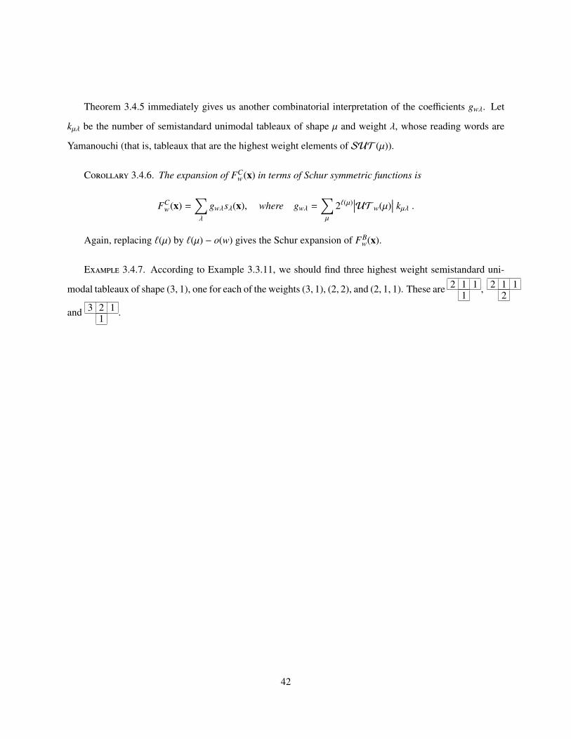
Theorem 3.4.5 immediately gives us another combinatorial interpretation of the coefficients gwλ. Let

kµλ be the number of semistandard unimodal tableaux of shape µ and weight λ, whose reading words are

Yamanouchi (that is, tableaux that are the highest weight elements of SUT (µ)).

Corollary 3.4.6. The expansion of FCw(x) in terms of Schur symmetric functions is

FCw(x) =

∑λ

gwλsλ(x), where gwλ =∑µ

2`(µ)∣∣∣UT w(µ)

∣∣∣ kµλ .

Again, replacing `(µ) by `(µ) − o(w) gives the Schur expansion of FBw(x).

Example 3.4.7. According to Example 3.3.11, we should find three highest weight semistandard uni-

modal tableaux of shape (3, 1), one for each of the weights (3, 1), (2, 2), and (2, 1, 1). These are 2 1 11

, 2 1 12

and 3 2 11

.

42

CHAPTER 4

Marked Tableaux of Staircase Shape: The Schur function sδ/µ

This chapter is based on the work in [Haw17].

4.1. Introduction

The ring of symmetric functions, Λ, has a Z-basis composed of Schur functions. Hence we can define

an invertible linear operator ω, by the formula ω(sλ) = sλ′ . We will call f ∈ Λ a fixed point of ω if

ω( f ) = f . Clearly sλ is a fixed point for any self-conjugate partition λ. Moreover, one can show that

ω(sλ/µ) = sλ′/µ′ , [Sta99] meaning that sλ/µ is a fixed point for any self-conjugate partitions µ ⊆ λ. In

particular sδ/µ, where δ = (n, n − 1, . . . 1) is a fixed point for any self-conjugate µ ⊆ δ. A priori there is little

reason to expect that for any µ ⊆ δ (not necessarily self-conjugate) sδ/µ would still be a fixed point. The

fact that δ is self-conjugate and ω(sλ/µ) = sλ′/µ′ means that the statement above is equivalent to sδ/µ = sδ/µ′ .

However, this will be an immediate consequence of the symmetry of generalized staircase tableaux.

Besides being a fixed point of ω, the function sδ/µ is interesting in its relation to shifted Schur functions.

For one, it is known, [AS12] that sδ/µ is P-Schur positive. We do not recreate this result here but do

obtain the result that sδ/µ(x1, x1, x2, x2, . . .) is Q-Schur positive. (Note that P-Schur positivity is immediately

guaranteed as a corollary of the result of [AS12], but not necessarily Q-Schur positivity.) In particular, we

derive that sδ/µ(x1, x1, x2, x2, . . .) is equal to a certain skew Q-Schur function, from which the result follows

by [Wor84], or [Ste89].

Our last application is deriving the equality of the skew Q-Schur functions Qλ+δ/µ+δ = Qλ′+δ/µ′+δ. On

the way to accomplishing this we define a t-deformation of Q-Schur functions and show that, in certain

cases, it is symmetric and Schur positive, and give a combinatorial interpretation of the Schur coefficients.

This is accomplished with the help of a certain crystal structure introduced in [HPS17]. We then prove that

certain permutations to the order of the alphabet 1′ < 1 < 2′ < 2 · · · , which is typically used to define

shifted semistandard tableaux (e.g. [Ser09]), may be made when the partition does not touch the diagonal.

43

Lastly, we note that the name generalized staircase tableaux (GST) is a bit deceptive, as we will de-

fine them for arbitrary shapes. However, non-staircase GST are simply used to aid in our proofs, and no

interesting results involve them.

4.2. Definitions

In what follows, we fix some n, and write δ = δ = (n, n − 1, . . . , 1). Any partition denoted by µ which

appears henceforth will be assumed to satisfy µ ⊆ δ. Moreover, whenever λ is mentioned we will assume

also that µ ⊆ λ and that l(λ) ≤ n.

A generalized staircase tableau (GST) of shape λ/µ and set I ⊆ N is a filling of the Young diagram λ/µ

with natural numbers such that:

(1) The rows and columns are weakly increasing.

(2) If i ∈ I then each row has at most one i.

(3) If i < I, then each column has at most one i.

Let G(λ/µ, I) denote the set of all GST of shape λ/µ and set I. For instance, G(λ/µ, ∅) is the set of skew

semistandard Young tableau of shape λ/µ, and the set G(λ/µ, 2N − 1) is in in bijection with the set of skew

shifted semi-standard tableaux of shape (δ + λ)/(δ + µ).

Suppose T is a GST of shape λ/µ . We will denote the box in row i and column j by bi j. We will denote

the value inside bi j by c(bi j) or by the “content of bi j.” For indexing purposes we will allow the coordinates

of i and j to be any non-negative integers, although box bi j is always empty whenever i = 0 or j = 0. We

define the content of these border boxes to be −∞. We also define an empty box inside of µ to have content

−∞. On the other hand, an empty box outside of λ (and with i and j positive) is defined to have content ∞.

The weight of T , denoted by wt(T ) is defined to be the vector whose ith coordinate is equal to the number of

is appearing in T .

Suppose that T is a GST of shape λ/µ and that bi j ∈ µ such that µ−{bi j} is a partition. We define forward

jdt into bi j as follows.

(1) Between the boxes bi( j+1) and b(i+1) j select the box whose content is lesser. If the contents are

equal, then select bi( j+1) if c(bi( j+1)) = c(b(i+1) j) ∈ I and b(i+1) j otherwise.

(2) If an empty box was selected, the algorithm terminates. Otherwise move the content of the selected

box into bi j.

44

(3) Re-index so that the newly emptied box is bi j and return to step 1.

Similarly, we define reverse jdt into a box bi j < λ such that λ ∪ {bi j} is a partition as follows:

(1) Between the boxes bi( j−1) and b(i−1) j select the box whose content is greater. If the contents are

equal, then select bi( j−1) if c(bi( j−1)) = c(b(i−1) j) ∈ I and b(i−1) j otherwise.

(2) If an empty box was selected, the algorithm terminates. Otherwise move the content of the selected

box into bi j.

(3) Re-index so that the newly emptied box is bi j and return to step 1.

Note that in both cases a valid GST is returned. Moreover, our jdt satisfies the familiar properties of

classic jdt:

J1 If T ′ is obtained from T by forward jdt into bi j, and bi′ j′ is the last box to be emptied, then T can

be obtained from T ′ by reverse jdt into bi′ j′ .

J2 If T ′ is obtained from T by reverse jdt into bi j, and bi′ j′ is the last box to be emptied, then T can

be obtained from T ′ by forward jdt into bi′ j′ .

J3 If i ≥ k and j < l and it is possible to forward jdt into bkl and then forward jdt into bi j, and the

boxes emptied by doing this are (in order) bk′l′ and bi′ j′ then i′ ≥ k′ and j′ < l′.

J4 If i < k and j ≥ l and it is possible to forward jdt into bkl and then forward jdt into bi j, and the

boxes emptied by doing this are (in order) bk′l′ and bi′ j′ then i′ < k′ and j′ ≥ l′.

J5 If i ≥ k and j < l and it is possible to reverse jdt into bi j and then reverse jdt into bkl, and the boxes

emptied by doing this are (in order) bi′ j′ and bk′l′ then i′ ≥ k′ and j′ < l′.

J6 If i < k and j ≥ l and it is possible to reverse jdt into bi j and then reverse jdt into bkl, and the boxes

emptied by doing this are (in order) bi′ j′ and bk′l′ then i′ < k′ and j′ ≥ l′.

4.3. Results

Theorem 4.3.1. If I and I′ are any subsets of the natural numbers, there is a weight preserving bijection

from G(δ/µ, I) to G(δ/µ, I′).

Proof. It suffices to show that for any I and any i < I there is a weight preserving bijection from

G(δ/µ, I) to G(δ/µ, I ∪ i). Let µ ⊆ ν ⊆ λ, be the partition consisting of all boxes of µ and all boxes of λ with

content less than i. It will suffice to find a weight-preserving bijection from G(δ/ν, I≥i) to G(δ/ν, I≥i ∪ i) or

equivalently from G(δ/ν, J) to G(δ/ν, J ∪ 1) where J = [(−i + 1) + I]≥1.

45

We therefore assume that in the statement of the theorem, i = 1 < I, and I′ = I ∪ 1. Let T ∈ G(δ/µ, I).

First erase all of the 1s which appear in T . The result is a horizontal strip of empty boxes on the inside of the

tableau. Now, forward jdt into each one of these empty boxes starting with the rightmost and moving left.

By property J3, the boxes which are emptied along the outside of the tableau will form a horizontal strip,

and they will be emptied from right to left. However, since δ is the staircase shape, this strip is in fact also

a vertical strip. Now, reverse jdt into each of the boxes of this vertical strip, starting with the highest and

moving down. By property J6, the boxes emptied along the inside of the tableau will form a vertical strip,

and they will be emptied starting with the highest and moving down. Put a 1 into each of the newly emptied

boxes. This produces a tableau in G(δ/µ, I∪1) which we define to be φ(T ). Now, given any T ∈ G(δ/µ, I∪1)

define φ−1(T ) = φ(T t)t, where the superscript t stands for row/column transposition. It is not hard to check

that φ−1(T ) ∈ G(δ/µ, I) and that both φ ◦ φ−1 = Id and φ−1 ◦ φ = Id.

�

Theorem 4.3.2. sδ/µ is a fixed point of the involution ω.

Proof. By the comments in the introduction, this is equivalent to showing that sδ/µ = sδ/µ′ . But this

equality is equivalent to the equality:

∑T∈G(δ/µ,∅)

xwt(T ) =∑

T∈G(δ/µ,N)

xwt(T ),

which is true because G(δ/µ, ∅) and G(δ/µ,N) are in weight preserving bijection.

�

Our next application relates Schur and Q-Schur functions of certain shapes: For our purposes we will

define a Q-tableau to be a filling of the shape λ/µ using letters from the ordered alphabet 1′ < 1 < 2′ < 2 . . .

such that:

(1) The rows and columns are weakly increasing.

(2) No primed number appears more than once in any row.

(3) No unprimed number appears more than once in any column.

We define the reading word of a Q-tableau to be the word obtained by reading the primed entries in T

down columns from right to left and then reading the the unprimed entries left to right across rows, starting

46

with the lowest row and working up. We consider this word as a word in the alphabet {1, 2, 3, . . .} by ignoring

the primes which appear above the entries at the beginning of the word. This is the same definition as for

the reading word of “primed tableaux” in [HPS17], except that here, our tableaux are not shifted.

We define a function:

Qtrλ/µ =

∑T

xwt(T )tP(T )rU(T ),

where the sum is over all Q-tableaux of shape λ/µ, where wt(T ) is the vector whose ith coordinate counts

the number of times either i or i′ appears in T , and where P(T ) (resp. U(T )) counts the number of times a

primed (resp. unprimed) entry appears in T . Notice that, by definition, Qtrλ/µ

at t = 1 = r is the Q-Schur

function Qλ+δ/µ+δ.

Theorem 4.3.3.

Qtrλ/µ =

∑k

(∑ν

cν,kλ/µ

sν

)tkr|λ|−|µ|−k

Where cν,kλ/µ

is the number of Q-tableau of shape λ/µ and weight ν which have exactly k of their entries

primed, and whose reading word is Yamanouchi.

Proof. The crystal operators on primed tableau given in [HPS17] induce crystal operators on skew

primed tableaux in the natural way. Notice that the set of skewed primed tableaux of shape λ + δ/µ + δ is

cannonically equivalent to the set of all Q-tableaux of shape λ/µ, and so we obtain a crystal structure on the

latter. Moreover, when the set of Q-tableaux of shape λ/µ inherits this structure, the highest weight elements

of this crystal will be those Q-tableaux whose reading word is Yamanouchi. This follows directly from the

description of highest weight primed tableaux given in [HPS17]. In order to prove the theorem, it remains

to show that P(T ) is constant on connected components of the induced crystal on Q-tableaux. However, one

may check that the crystal operator fi in [HPS17] preserves the number of primes in a given primed tableau

whenever this tableau has no is or (i+1)s on the diagonal. However, note that we are associating Q-tableaux

of shape λ/µ to primed tableaux of shifted skew shape λ + δ/µ + δ, and that the latter shape has no boxes

on the diagonal. Thus, it is the case that for all i, we are always applying the operator fi to a (skew) primed

tableaux with no is or (i + 1)s on the diagonal. Thus, the induced operators on Q-tableaux also preserve the

number of primes in a given Q-tableau. �

47

Theorem 4.3.4.

sδ/µ(tx1, rx1, tx2, rx2, . . .) = Qtrδ/µ =

∑k

(∑ν

cν,kδ/µ

sν

)tkr|δ|−|µ|−k

In particular, sδ/µ(x1, x1, x2, x2, . . .) is Q-Schur positive (since it is equal to the skew Q-Schur function

Qλ+δ/µ+δ which is Q-Schur positive by [Wor84] or [Ste89]), and we have that sδ/µ(tx1, x1, tx2, x2, . . .) is

Schur positive.

Proof.

sδ/µ(tx1, rx1, tx2, rx2, . . .) =∑

T

xwt(T )tP(T )r|δ|−|µ|−P(T ),

where we claim the sum can be taken over any of the following:

(1) Over all SSYT of shape δ/µ, where wt(T ) is the vector whose ith coordinate counts the number of

times either 2i − 1 or 2i appears in T , and where P(T ) counts the number of times an odd entry

appears in T .

(2) Over G(δ/µ, ∅), where wt(T ) is the vector whose ith coordinate counts the number of times either

2i − 1 or 2i appears in T , and where P(T ) counts the number of times an odd entry appears in T .

(3) Over G(δ/µ, 2N − 1), where wt(T ) is the vector whose ith coordinate counts the number of times

either 2i − 1 or 2i appears in T , and where P(T ) counts the number of times an odd entry appears

in T .

(4) Over all Q-tableaux of shape δ/µ, where wt(T ) is the vector whose ith coordinate counts the number

of times either i or i′ appears in T , and where P(T ) counts the number of times a primed entry

appears in T .

(1) is true by definition. (1) =⇒ (2) by the definition of GST. (2) =⇒ (3) by 4.3.1. (3) =⇒ (4) by

relabeling the alphabet, and (4) corresponds to the statement in the theorem.

�

Corollary 4.3.5. Qtrδ/µ

is symmetric in t and r, and Qtrδ/µ

= Qtrδ/µ′

. In particular, we have the equality of

skew Q-Schur functions Qδ+δ/µ+δ = Qδ+δ/µ′+δ.

In fact, more generally we have:

48

Proposition 4.3.6. Qtrλ/µ

(x; t, r) = Qtrλ′/µ′

(x; r, t).

Before proving this, we introduce a generalization of Q-tableau. Let I ⊆ N and define the total order ≤I

on the alphabet {1′, 1, 2′, 2, . . .} by

(1) If i < j then i <I j, i <I j′, i′ <I j, i′ <I j′

(2) If i ∈ I then i <I i′

(3) If i < I then i′ <I i

We define a generalized Q-tableau of shape λ/µ and set I to be a filling of this shape using {1′, 1, 2′, 2, . . .}

such that:

(1) The rows and columns are weakly increasing under ≤I .

(2) No primed number appears more than once in any row.

(3) No unprimed number appears more than once in any column.

The set of all such tableaux is denoted Q(λ/µ, I).

Theorem 4.3.7. For any subsets of the natural numbers, I, and I′, there is a bijection from Q(λ/µ, I) to

Q(λ/µ, I′) which preserves wt(T ) and P(T ).

Proof. It suffices to suppose that I′ = I∪ i for some i < I. Let T ∈ Q(λ/µ, I) and define ψ(T ) as follows.

First, write down T . Notice that the is and i′s in T form a set of connected ribbons. Within each of these

connected ribbons, cycle every entry one position: to the left if the box to its left is in the ribbon, downwards

if the box below it is in the ribbon, or, if neither is the case, i.e., it is at the bottom left end of the ribbon,

move it to the upper right end of the ribbon. ψ−1 is defined similarly, but by cycling the other direction. �

We can now prove 4.3.6.

Proof. We seek a weight preserving bijection from Q(λ′/µ′, ∅) to Q(λ/µ, ∅) which interchanges P(T )

and U(T ). Let T ∈ Q(λ′/µ′, ∅). Tranpose T and then prime the unprimed elements and unprime the primed

elements. This gives a weight preserving bijection from Q(λ′/µ′, ∅) to Q(λ/µ,N) which interchanges P(T )

and U(T ), and by 4.3.7, this is sufficient. �

Corollary 4.3.8. We have the equality of skew Q-Schur functions Qλ+δ/µ+δ = Qλ′+δ/µ′+δ.

(Here we make the additional assumption that λ1 ≤ n.)

49

CHAPTER 5

Primed Tableaux of Shifted Shape Revisited: Crystal Characterization

This chapter is based on a portion of the work in [GHPS18].

5.1. Introduction

One of the major advances in the theory of crystals for simply-laced Lie algebras was the discovery

by Stembridge [Ste03] of local axioms that uniquely characterize the crystal graphs corresponding to Lie

algebra representations. These local axioms provide a completely combinatorial approach to the theory of

crystals; this viewpoint was taken in [BS17].

A theory of highest weight crystals for the queer superalgebra q(n) was recently developed by Grantcharov

et al. [GJK+15]. They provide an explicit combinatorial realization of the highest weight crystal bases in

terms of semistandard decomposition tableaux and show how these crystals can be derived from a tensor

product rule and the vector representation. Independently, Hiroshima [Hir18] and Assaf and Oguz [AKO18a,

AKO18b] defined a queer crystal structure on semistandard shifted tableaux, extending the type A crystal

structure of [HPS17] on these tableaux.

In this chapter, we provide a characterization of the queer supercrystals in analogy to Stembridge’s [Ste03]

characterization of crystals associated to classical simply-laced root systems. Assaf and Oguz [AKO18a,

AKO18b] conjecture a local characterization of queer crystals in the spirit of Stembridge [Ste03], which

involves local relations between the odd crystal operator f−1 with the type An−1 crystal operators fi for

1 6 i < n. However, we provide a counterexample to [AKO18b, Conjecture 4.16], which conjectures

that these local axioms uniquely characterize the queer supercrystals. Instead, we define a new graph G(C)

on the relations between the type A components of the queer supercrystal C, which together with Assaf’s

and Oguz’ local queer axioms and further new axioms uniquely fixes the queer crystal structure (see Theo-

rem 5.5.1). We provide a combinatorial description of G(C) by providing the combinatorial rules for all odd

queer crystal operators f−i and e−i on certain highest weight elements for 1 6 i < n.

50

This chapter is structured as follows. In Section 5.2, we review the combinatorial definition of the queer

supercrystals by [GJK+15]. In Section 5.3, we state the local queer axioms by Assaf and Oguz [AKO18a,

AKO18b] and provide a counterexample to [AKO18b, Conjecture 4.16]. The graph G(C) is introduced in

Section 5.4 which together with the local queer axioms of Definition 5.3.1 and new connectivity axioms of

Definition 5.4.3 uniquely characterize the queer crystals as stated in Theorem 5.5.1.

5.2. Queer supercrystals

5.2.1. Definition of queer supercrystals. An (abstract) crystal of type An is a nonempty set B together

with the maps

ei, fi : B→ B t {0} for i ∈ I,

wt : B→ Λ,

(5.1)

where Λ = Zn+1>0 is the weight lattice of the root of type An and I = {1, 2, . . . , n} is the index set, subject to

several conditions. Denote by αi = εi − εi+1 for i ∈ I the simple roots of type An, where εi is the i-th standard

basis vector of Zn+1. Then we require:

A1. For b, b′ ∈ B, we have fib = b′ if and only if b = eib′. In this case wt(b′) = wt(b) − αi.

For b ∈ B, we also define

ϕi(b) = max{k ∈ Z>0 | f ki (b) , 0} and εi(b) = max{k ∈ Z>0 | ek

i (b) , 0}.

For further details, see for example [BS17, Definition 2.13].

There is an action of the symmetric group S n on a type An crystal B given by the operators

(5.2) si(b) =

f ki (b) if k > 0,

e−ki (b) if k < 0,

for b ∈ B, where k = ϕi(b) − εi(b).

An element b ∈ B is called highest weight if ei(b) = 0 for all i ∈ I. Similarly, b is called lowest weight

if fi(b) = 0 for all i ∈ I. For a subset J ⊆ I, we say that b is J-highest weight if ei(b) = 0 for all i ∈ J and

similarly b is J-lowest weight if fi(b) = 0 for all i ∈ J.

We are now ready to define an abstract queer crystal.

51

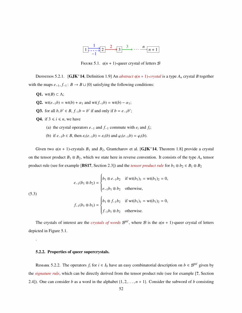
1 2 3 . . . n + 11

−1

2 3 n

Figure 5.1. q(n + 1)-queer crystal of letters B

Definition 5.2.1. [GJK+14, Definition 1.9] An abstract q(n + 1)-crystal is a type An crystal B together

with the maps e−1, f−1 : B→ B t {0} satisfying the following conditions:

Q1. wt(B) ⊂ Λ;

Q2. wt(e−1b) = wt(b) + α1 and wt( f−1b) = wt(b) − α1;

Q3. for all b, b′ ∈ B, f−1b = b′ if and only if b = e−1b′;

Q4. if 3 6 i 6 n, we have

(a) the crystal operators e−1 and f−1 commute with ei and fi;

(b) if e−1b ∈ B, then εi(e−1b) = εi(b) and ϕi(e−1b) = ϕi(b).

Given two q(n + 1)-crystals B1 and B2, Grantcharov et al. [GJK+14, Theorem 1.8] provide a crystal

on the tensor product B1 ⊗ B2, which we state here in reverse convention. It consists of the type An tensor

product rule (see for example [BS17, Section 2.3]) and the tensor product rule for b1 ⊗ b2 ∈ B1 ⊗ B2

e−1(b1 ⊗ b2) =

b1 ⊗ e−1b2 if wt(b1)1 = wt(b1)2 = 0,

e−1b1 ⊗ b2 otherwise,

f−1(b1 ⊗ b2) =

b1 ⊗ f−1b2 if wt(b1)1 = wt(b1)2 = 0,

f−1b1 ⊗ b2 otherwise.

(5.3)

The crystals of interest are the crystals of words B⊗`, where B is the q(n + 1)-queer crystal of letters

depicted in Figure 5.1.

.

5.2.2. Properties of queer supercrystals.

Remark 5.2.2. The operators fi for i ∈ I0 have an easy combinatorial description on b ∈ B⊗` given by

the signature rule, which can be directly derived from the tensor product rule (see for example [?, Section

2.4]). One can consider b as a word in the alphabet {1, 2, . . . , n + 1}. Consider the subword of b consisting

52

only of the letters i and i + 1. Pair (or bracket) any consecutive letters i + 1, i in this order, remove this pair,

and repeat. Then fi changes the rightmost unpaired i to i + 1; if there is no such letter fi(b) = 0. Similarly,

ei changes the leftmost unpaired i + 1 to i; if there is no such letter ei(b) = 0.

Remark 5.2.3. From (5.3), one may also derive a simple combinatorial rule for f−1 and e−1. Consider

the subword v of b ∈ B⊗` consisting of the letters 1 and 2. The crystal operator f−1 on b is defined if the

leftmost letter of v is a 1, in which case it turns it into a 2. Otherwise f−1(b) = 0. Similarly, e−1 on b is

defined if the leftmost letter of v is a 2, in which case it turns it into a 1. Otherwise e−1(b) = 0.

5.3. Local axioms

In [AKO18b, Definition 4.11], Assaf and Oguz give a definition of regular queer crystals. In essence,

their axioms are rephrased in the following definition, where I := I0 ∪ {−1}.

Definition 5.3.1. Let C be a graph with labeled directed edges given by fi for i ∈ I0 and f−1. If b′ = f jb

for j ∈ I define e j by b = e jb′.

LQ1. The subgraph with all vertices but only edges labeled by i ∈ I0 is a type An Stembridge crystal.

LQ2. ϕ−1(b), ε−1(b) ∈ {0, 1} for all b ∈ C.

LQ3. ϕ−1(b) + ε−1(b) > 0 if wt(b)1 + wt(b)2 > 0.

LQ4. Assume ϕ−1(b) = 1 for b ∈ C.

(a) If ϕ1(b) > 2, we have

f1 f−1(b) = f−1 f1(b),

ϕ1(b) = ϕ1( f−1(b)) + 2,

ε1(b) = ε1( f−1(b)).

(b) If ϕ1(b) = 1, we have

f1(b) = f−1(b).

LQ5. Assume ϕ−1(b) = 1 for b ∈ C.

53

(a) If ϕ2(b) > 0, we have

f2 f−1(b) = f−1 f2(b),

ϕ2(b) = ϕ2( f−1(b)) − 1,

ε2(b) = ε2( f−1(b)).

(b) If ϕ2(b) = 0, we have

ϕ2(b) = ϕ2( f−1(b)) − 1 = 0, or ϕ2(b) = ϕ2( f−1(b)) = 0,

ε2(b) = ε2( f−1(b)), ε2(b) = ε2( f−1(b)) + 1.

LQ6. Assume that ϕ−1(b) = 1 and ϕi(b) > 0 with i > 3 for b ∈ C. Then

fi f−1(b) = f−1 fi(b),

ϕi(b) = ϕi( f−1(b)),

εi(b) = εi( f−1(b)).

Proposition 5.3.2 ( [AKO18b]). The queer crystal of words B⊗` satisfies the axioms in Definition 5.3.1.

Proof. This can easily checked using the combinatorial interpretation of the operators outlined in the

remarks above. �

In [AKO18b, Conjecture 4.16], Assaf and Oguz conjecture that every regular queer crystal is a normal

queer crystal. In other words, every connected graph satisfying the local queer axioms of Definition 5.3.1 is

isomorphic to a connected component in someB⊗`. We provide a counterexample to this claim in Figure 5.2.

In the figure, the I0-components of the q(3)-crystal of highest weight (4, 2, 0) are shown. Some of the f−1-

arrows are drawn in green. The remaining arrows can be filled in using the axioms of local queer axioms

in a consistent manner. If the dashed green arrow from 331131 to 332131 and the dashed green arrow

from 331132 to 332132 are replaced by the dashed purple arrow from 331131 to 331231 and the dashed

purple arrow from 331132 to 332231, respectively, all axioms of Definition 5.3.1 are still satisfied with the

remaining f−1-arrows filled in. However, the I0-component with highest weight element 132121 has become

disconnected and hence the two crystals are not isomorphic.

54

1⊗

3⊗

1⊗

1⊗

2⊗

1

2⊗

2⊗

1⊗

2⊗

3⊗

2

3⊗

3⊗

2⊗

2⊗

3⊗

1

1⊗

3⊗

1⊗

3⊗

3⊗

1

2⊗

3⊗

2⊗

3⊗

3⊗

2

1⊗

3⊗

1⊗

2⊗

2⊗

1

3⊗

3⊗

1⊗

1⊗

3⊗

2

1⊗

3⊗

1⊗

1⊗

3⊗

1

2⊗

2⊗

1⊗

3⊗

3⊗

1

1⊗

2⊗

1⊗

2⊗

3⊗

1

2⊗

2⊗

1⊗

1⊗

2⊗

1

3⊗

3⊗

1⊗

2⊗

3⊗

2

2⊗

3⊗

1⊗

2⊗

2⊗

12⊗

3⊗

2⊗

1⊗

2⊗

1

3⊗

3⊗

2⊗

3⊗

3⊗

1

1⊗

3⊗

2⊗

1⊗

3⊗

2

3⊗

3⊗

1⊗

1⊗

2⊗

1

1⊗

2⊗

1⊗

3⊗

3⊗

2

3⊗

3⊗

1⊗

3⊗

3⊗

12⊗

3⊗

2⊗

2⊗

3⊗

2

2⊗

3⊗

1⊗

3⊗

3⊗

1

3⊗

3⊗

2⊗

2⊗

3⊗

2

1⊗

3⊗

2⊗

3⊗

3⊗

2

1⊗

3⊗

1⊗

1⊗

3⊗

2

3⊗

3⊗

1⊗

3⊗

3⊗

2

2⊗

3⊗

2⊗

3⊗

3⊗

1

1⊗

3⊗

2⊗

2⊗

2⊗

1

2⊗

3⊗

1⊗

1⊗

3⊗

2

2⊗

3⊗

1⊗

2⊗

3⊗

2

1⊗

3⊗

1⊗

2⊗

3⊗

2

3⊗

3⊗

2⊗

1⊗

3⊗

12⊗

3⊗

2⊗

1⊗

3⊗

2

1⊗

3⊗

2⊗

2⊗

3⊗

1

1⊗

2⊗

1⊗

1⊗

3⊗

1

3⊗

3⊗

2⊗

3⊗

3⊗

2

2⊗

3⊗

1⊗

1⊗

2⊗

1

3⊗

3⊗

2⊗

1⊗

2⊗

12⊗

3⊗

2⊗

2⊗

2⊗

1

2⊗

2⊗

1⊗

1⊗

3⊗

2

3⊗

3⊗

1⊗

2⊗

3⊗

12⊗

3⊗

2⊗

2⊗

3⊗

1

2⊗

3⊗

1⊗

3⊗

3⊗

2

1⊗

2⊗

1⊗

1⊗

2⊗

1

2⊗

3⊗

1⊗

1⊗

3⊗

11⊗

2⊗

1⊗

3⊗

3⊗

1

3⊗

3⊗

2⊗

1⊗

3⊗

2

1⊗

3⊗

2⊗

1⊗

3⊗

1

1⊗

3⊗

1⊗

3⊗

3⊗

2

2⊗

2⊗

1⊗

1⊗

3⊗

1

2⊗

3⊗

1⊗

2⊗

3⊗

12⊗

3⊗

2⊗

1⊗

3⊗

1

1⊗

3⊗

2⊗

1⊗

2⊗

1

3⊗

3⊗

1⊗

2⊗

2⊗

1

2⊗

2⊗

1⊗

3⊗

3⊗

2

1⊗

2⊗

1⊗

1⊗

3⊗

2

1⊗

2⊗

1⊗

2⊗

3⊗

22⊗

2⊗

1⊗

2⊗

3⊗

1

1⊗

3⊗

2⊗

3⊗

3⊗

11⊗

3⊗

2⊗

2⊗

3⊗

2

1⊗

2⊗

1⊗

2⊗

2⊗

1

1⊗

3⊗

1⊗

2⊗

3⊗

1

3⊗

3⊗

2⊗

2⊗

2⊗

1

2⊗

2⊗

1⊗

2⊗

2⊗

1

3⊗

3⊗

1⊗

1⊗

3⊗

1

21

2

2

2

−1

1

2

2

1

−1

1

1

2

2

2

1

1

2

2

1

1

11

2

2

2

1

2

1

22

2

1

2

2

1

12

1

1

2

1

1

2

21

2

111

1

12

2

12

2

1

1

21

2

1

2

1

−1

2

2

1

12

1

2

1

1

1

22

−1

−1

−1

−1

−1

Figure 5.2. Counterexample to the unique characterization of the local queer axioms ofDefinition 5.3.1.

55

The problem is demonstrated by the counterexample in Figure 5.2: switching components with the same

I0-highest weights can cause non-uniqueness. In fact, if f−1b is determined for all b ∈ C such that

(5.1) ϕi(b) = 0 for all i ∈ I0 \ {1} and ϕ1(b) = 2,

then, by the relations between f−1 and fi for i ∈ I0 of Definition 5.3.1, f−1 is determined on all elements in

C.

Lemma 5.3.3. Let v ∈ B⊗` be an I0-lowest weight element, that is, ϕi(v) = 0 for all i ∈ I0. Then every

b ∈ B⊗` satisfying (5.1) is of the form

(5.2) g j,k := (e1 · · · e j)(e1 · · · ek)v for some 1 6 j 6 k 6 n.

Conversely, every g j,k , 0 with 1 6 j 6 k 6 n satisfies (5.1).

Proof. The statement of the lemma is a statement about type An crystals and hence can be verified by

the tableaux model for type An crystals (see for example [BS17]). The element v is I0-lowest weight and

hence as a tableau in French notation contains the letter n + 1 at the top of each column, the letter n in

the second to top box in each column, and in general the letter n + 2 − i in the i-th box from the top in its

column. If there is a letter k + 1 in the first row of v, then (e1 · · · ek) applies to v and b′ = (e1 · · · ek)v satisfies

ϕi(b′) = 0 for i ∈ I0 \ {1} and ϕ1(b′) = 1. The element b′ has several changed entries in the first row, and

otherwise the entries above the first row all have letter n + 2 − i in the i-th box from the top in their column.

If b′ has a letter j + 1 in the first row with 1 6 j 6 k, then (e1 · · · e j) applies to b′ and b = g j,k = (e1 · · · e j)b′

satisfies (5.1). Note that if j > k, then the last e1 would no longer apply and hence b = 0. This proves that

g j,k , 0 as in (5.2) satisfies (5.1). If conversely b satisfies (5.1), then as a tableau it contains two extra 1’s

in the first row that have a 3 or bigger above them rather than a 2 in their columns, and for entries higher

than the first row the i-th box from the top in its column contains n + 2 − i. It is not hard to check that then

( fk · · · f1)( f j · · · f1)b = v for some 1 6 j 6 k 6 n. Hence b is of the form (5.2). �

In the next section, we introduce a new graph just on I0-highest weight elements and new connectivity

axioms (see Definition 5.4.3) that uniquely characterizes queer crystals (see Theorem 5.5.1).

56

5.4. Graph on type A components

Let C be a crystal with index set I0 ∪ {−1} that is a Stembridge crystal of type An when restricted to

the arrows labeled I0. In this section, we define a graph for C labeled by the type An components of C. We

draw an edge from vertex C1 to vertex C2 in this graph if there is an element b1 in the component C1 and an

element b2 in the component C2 such that f−1b1 = b2. We also provide new axioms in Definition 5.4.3 that

will be used in Section 5.5 to provide a unique characterization of queer crystals.

Definition 5.4.1. Let C be a crystal with index set I0∪{−1} that is a Stembridge crystal of type An when

restricted to the arrows labeled I0. We define the component graph of C, denoted by G(C), as follows. The

vertices of G(C) are the type An components of C (typically labeled by their highest weight elements). There

is an edge from vertex C1 to vertex C2 in this graph, if there is an element b1 in the component C1 and an

element b2 in the component C2 such that

f−1b1 = b2.

Example 5.4.2. Let C be the connected component in the q(3)-crystal B⊗6 with highest weight element

1⊗2⊗1⊗1⊗2⊗1 of highest weight (4, 2, 0). The graph G(C) is given in Figure 5.3 on the left (disregarding

the labels on the edges). The graph G(C′) for the counterexample C′ in Figure 5.2 is given in Figure 5.3 on

the right. Since the two graphs are not isomorphic as unlabeled graphs, this confirms that the purple dashed

arrows in Figure 5.2 do not give the queer crystal even though the induced crystal satisfies the axioms in

Definition 5.3.1.

Next we introduce new axioms.

Definition 5.4.3. Let C be a connected crystal satisfying the local queer axioms of Definition 5.3.1.

Let v ∈ C be an I0-lowest weight element and u =↑ v. As in (5.2), define g j,k := (e1 · · · e j)(e1 · · · ek)v for

1 6 j 6 k 6 n.

C0. ϕ−1(g j,k) = 0 implies that ϕ−1(e1 · · · ekv) = 0.

C1. Suppose that G(C) contains an edge u → u′ such that wt(u′) is obtained from wt(u) by moving a

box from row n + 1− k to row n + 1− h with h < k. For all h < j 6 k such that g j,k , 0, we require

that f−1g j,k , 0 and

f−1g j,k = (e2 · · · e j)(e1 · · · eh)v′,

57

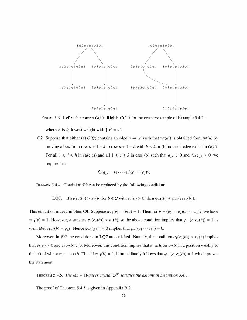
3 ⊗ 3 ⊗ 2 ⊗ 1 ⊗ 2 ⊗ 1

2 ⊗ 3 ⊗ 1 ⊗ 1 ⊗ 2 ⊗ 1

2 ⊗ 2 ⊗ 1 ⊗ 1 ⊗ 2 ⊗ 1

1 ⊗ 3 ⊗ 2 ⊗ 1 ⊗ 2 ⊗ 1

1 ⊗ 3 ⊗ 1 ⊗ 1 ⊗ 2 ⊗ 1

1 ⊗ 2 ⊗ 1 ⊗ 1 ⊗ 2 ⊗ 1

3 ⊗ 3 ⊗ 2 ⊗ 1 ⊗ 2 ⊗ 1

2 ⊗ 3 ⊗ 1 ⊗ 1 ⊗ 2 ⊗ 1

2 ⊗ 2 ⊗ 1 ⊗ 1 ⊗ 2 ⊗ 1

1 ⊗ 3 ⊗ 2 ⊗ 1 ⊗ 2 ⊗ 1

1 ⊗ 3 ⊗ 1 ⊗ 1 ⊗ 2 ⊗ 1

1 ⊗ 2 ⊗ 1 ⊗ 1 ⊗ 2 ⊗ 1

Figure 5.3. Left: The correct G(C). Right: G(C′) for the counterexample of Example 5.4.2.

where v′ is I0-lowest weight with ↑ v′ = u′.

C2. Suppose that either (a) G(C) contains an edge u → u′ such that wt(u′) is obtained from wt(u) by

moving a box from row n + 1 − k to row n + 1 − h with h < k or (b) no such edge exists in G(C).

For all 1 6 j 6 h in case (a) and all 1 6 j 6 k in case (b) such that g j,k , 0 and f−1g j,k , 0, we

require that

f−1g j,k = (e2 · · · ek)(e1 · · · e j)v.

Remark 5.4.4. Condition C0 can be replaced by the following condition:

LQ7. If ε1(e2(b)) > ε1(b) for b ∈ C with ε2(b) > 0, then ϕ−1(b) 6 ϕ−1(e1e2(b)).

This condition indeed implies C0. Suppose ϕ−1(e1 · · · ekv) = 1. Then for b = (e3 · · · e j)(e1 · · · ek)v, we have

ϕ−1(b) = 1. However, b satisfies ε1(e2(b)) > ε1(b), so the above condition implies that ϕ−1(e1e2(b)) = 1 as

well. But e1e2(b) = g j,k. Hence ϕ−1(g j,k) = 0 implies that ϕ−1(e1 · · · ekv) = 0.

Moreover, in B⊗` the conditions in LQ7 are satisfied. Namely, the condition ε1(e2(b)) > ε1(b) implies

that e2(b) , 0 and e1e2(b) , 0. Moreover, this condition implies that e1 acts on e2(b) in a position weakly to

the left of where e2 acts on b. Thus if ϕ−1(b) = 1, it immediately follows that ϕ−1(e1e2(b)) = 1 which proves

the statement.

Theorem 5.4.5. The q(n + 1)-queer crystal B⊗` satisfies the axioms in Definition 5.4.3.

The proof of Theorem 5.4.5 is given in Appendix B.2.

58

5.5. Characterization of queer crystals

Our main theorem gives a characterization of the queer supercrystals.

Theorem 5.5.1. Let C be a connected component of a generic abstract queer crystal (see Defini-

tion 5.2.1). Suppose that C satisfies the following conditions:

(1) C satisfies the local queer axioms of Definition 5.3.1.

(2) C satisfies the connectivity axioms of Definition 5.4.3.

(3) G(C) is isomorphic to G(D), whereD is some connected component of B⊗`.

Then the queer supercrystals C andD are isomorphic.

Theorem 5.5.1 states that the local queer axioms, the connectivity axioms, and the component graph

uniquely characterize queer crystals. Before we give its proof, we need the following statement. Recall that

g j,k = (e1 · · · e j)(e1 · · · ek)v was defined in (5.2), where v is an I0-lowest weight vector.

Lemma 5.5.2. In a crystal satisfying the local queer axioms of Definition 5.3.1 and C0 of Definition 5.4.3,

we have for any g j,k , 0 with 1 6 j 6 k

ϕ−1(g j,k) = 0 if and only if ϕ−1(e1 · · · ekv) = 0.

Proof. The condition C0 requires that ϕ−1(g j,k) = 0 implies ϕ−1(e1 · · · ekv) = 0.

For the converse direction, note that wt(e1 · · · ekv)1 > 0. Hence

ϕ−1(e1 · · · ekv) = 0 ⇔ ε−1(e1 · · · ekv) = 1.

By the local queer axioms LQ6 and LQ5 of Definition 5.3.1 (see also Figure ??), we have

ε−1(e1 · · · ekv) = 1 ⇔ ε−1((e3 · · · e j)(e1 · · · ek)v) = 1 ⇒ ε−1((e2 · · · e j)(e1 · · · ek)v) = 1.

It can be easily checked that ϕ1((e2 · · · e j)(e1 · · · ek)v) = 1 for j 6 k (for example using the tableaux model

for type An crystals). Hence by the local queer axioms

ε−1((e2 · · · e j)(e1 · · · ek)v) = 1 ⇔ ε−1((e1 · · · e j)(e1 · · · ek)v) = 1.

This proves that ϕ−1(e1 · · · ekv) = 0 implies ϕ−1(g j,k) = 0. �

59

APPENDIX A

Appendix 1: Proofs for Type A crystal on primed tableaux

A.1.

In this appendix, we provide the proof of Theorem 3.3.3.

A.1.1. Preliminaries. We use the fact from [Hai89] that taking only elements smaller or equal to i + 1

from the word b and applying the mixed insertion corresponds to taking only the part of the tableau T with

elements 6 i+1. Thus, it is enough to prove the theorem for a “truncated” word b without any letters greater

than i + 1. To shorten the notation, we set j = i + 1 in this appendix. We sometimes also restrict to just the

letters i and j in a word w. We call this the {i, j}-subword of w.

First, in Lemma A.1.1 we justify the notion of the reading word rw(T) and provide the reason to use

a bracketing rule on it. After that, in Section A.1.2 we prove that the action of the crystal operator fi on b

corresponds to the action of fi on T after the insertion.

Given a word b, we apply the crystal bracketing rule for its {i, j}-subword and globally declare the

rightmost unbracketed i in b (i.e. the letter the crystal operator fi acts on) to be a bold i. Insert the letters of

b via Haiman insertion to obtain the insertion tableau T. During this process, we keep track of the position

of the bold i in the tableau via the following rules. When the bold i from b is inserted into T, it is inserted as

the rightmost i in the first row of T since by definition it is unbracketed in b and hence cannot bump a letter

j. From this point on, the tableau T has a special letter i and we track its position:

(1) If the special i is unprimed, it is always the rightmost i in its row. When a letter i is bumped from

this row, only one of the non-special letters i can be bumped, unless the special i is the only i in the

row. When the non-diagonal special i is bumped from its row to the next row, it will be inserted as

the rightmost i in the next row.

(2) When the diagonal special i is bumped from its row to the column to its right, it is inserted as the

bottommost i′ in the next column.

60

(3) If the special i is primed, it is always the bottommost i′ in its column. When a letter i′ is bumped

from this column, only one of the non-special letters i′ can be bumped, unless the special i′ is the

only i′ in the column. When the primed special i is bumped from its column to the next column, it

is inserted as the bottommost i′ in the next column.

(4) When i is inserted into a row with the special unprimed i, the rightmost i becomes special.

(5) When i′ is inserted into a column with the special primed i, the bottommost primed i becomes

special.

Lemma A.1.1. Using the rules above, after the insertion process of b, the special i in T is the same as

the rightmost unbracketed i in the reading word rw(T) (i.e. the definition of the bold i in T). Moreover, the

number of unbracketed letters i in b is equal to the number of unbracketed letters i in rw(T).

Proof. First, note that since both the number of letters i and the number of letters j are equal in b and

rw(T), the fact that the number of unbracketed letters i is the same implies that the number of unbracketed

letters j must also be the same. We use induction on 1 6 s 6 h, where the letters b1 . . . bs of b = b1b2 . . . bh

have been inserted using Haiman mixed insertion with the above rules. That is, we check that at each step

of the insertion algorithm the statement of our lemma stays true.

The induction step is as follows: Consider the word b1 . . . bs−1 with a corresponding insertion tableau

T(s−1). If the bold i in b is not in b1 . . . bs−1, then T(s−1) does not contain a special letter i. Otherwise,

by induction hypothesis assume that the bold i in b1 . . . bs−1 by the above rules corresponds to the special

i in T(s−1), that is, it is in the position corresponding to the rightmost unbracketed i in the reading word

rw(T(s−1)). Then we need to prove that for b1 . . . bs, the special i in T(s−1) ends up in the position corre-

sponding to the rightmost unbracketed i in the reading word of T(s) = T(s−1) f bs. We also need to verify

that the second part of the lemma remains true for T(s).

Remember that we are only considering “truncated” words b with all letters 6 j.

Case 1. Suppose bs = j. In this case j is inserted at the end of the first row of T(s−1), and rw(T(s)) has j

attached at the end. Thus, both statements of the lemma are unaffected.

Case 2. Suppose bs = i and bs is unbracketed in b1 . . . bs−1bs. Then there is no special i in tableau T(s−1),

and bs might be the bold i of the word b. Also, there are no unbracketed letters j in b1 . . . bs−1, and thus all

j in rw(T(s−1)) are bracketed. Thus, there are no letters j in the first row of T(s−1), and i is inserted in the

61

first row of T(s−1), possibly bumping the letter j′ from column c into an empty column c + 1 in the process.

Note that if j′ is bumped, moving it to column c + 1 of T(s) does not change the reading word, since column

c of T(s−1) does not contain any primed letters other than j′. The reading word of T(s) is thus the same as

rw(T(s−1)) except for an additional unbracketed i at the end. The number of unbracketed letters i in both

rw(T(s)) and b1 . . . bs−1bs is thus increased by one compared to rw(T(s−1)) and b1 . . . bs−1. If bs is the bold i

of the word b, the special i of tableau T(s) is the rightmost i on the first row and corresponds to the rightmost

unbracketed i in rw(T(s)).

Case 3. Suppose bs = i and bs is bracketed with a j in the word b1 . . . bs−1. In this case, according to the

induction hypothesis, rw(T(s−1)) has an unbracketed j. There are two options.

Case 3.1. If the first row of T(s−1) does not contain j, bs is inserted at the end of the first row of T(s−1),

possibly bumping j′ in the process. Regardless, rw(T(s)) does not change except for attaching an i at the end

(see Case 2). This i is bracketed with one unbracketed j in rw(T(s)). The special i (if there was one in T(s−1))

does not change its position and the statement of the lemma remains true.

Case 3.2. If the first row of T(s−1) does contain a j, inserting bs into T(s−1) bumps j (possibly bumping j′

beforehand) into the second row, where j is inserted at the end of the row. So, if the first row contains n > 0

elements i and m > 1 elements j, the reading word rw(T(s−1)) ends with . . . in jm, and rw(T(s)) ends with

. . . jin+1 jm−1. Thus, the number of unbracketed letters i does not change and if there was a special i in the

first row, it remains there and it still corresponds to the rightmost unbracketed i in rw(T(s)).

Case 4. Suppose bs < i. Inserting bs could change both the primed reading word and unprimed reading

word of T(s−1). As long as neither i nor j is bumped from the diagonal, we can treat primed and unprimed

changes separately.

Case 4.1. Suppose neither i nor j is not bumped from the diagonal during the insertion. This means that

there are no transitions of letters i or j between the primed and the unprimed parts of the reading word.

Thus, it is enough to track the bracketing relations in the unprimed reading word; the bracketing relations

in the primed reading word can be verified the same way via the transposition. After we make sure that the

number of unbracketed letters i and j changes neither in the primed nor unprimed reading word, it is enough

to consider the case when the special i is unprimed, since the case when it is primed can again be checked

62

using the transposition. To avoid going back and forth, we combine these two processes together in each

subcase to follow.

Case 4.1.1. If there are no letters i and j in the bumping sequence, the unprimed {i, j}-subword of rw(T(s))

is the same as in rw(T(s−1)). The special i (if there is one) remains in its position, and thus the statement of

the lemma remains true.

Case 4.1.2. Now consider the case when there is a j in the bumping sequence, but no i. Let that j be bumped

from the row r. Since there is no i bumped, row r does not contain any letters i. Thus, bumping j from row

r to the end of row r + 1 does not change the {i, j}-subword of rw(T(s−1)), so the statement of the lemma

remains true.

Case 4.1.3. Consider the case when there is an i in the bumping sequence. Let that i be bumped from the

row r.

Case 4.1.3.1. If there is a (non-diagonal) j in row r + 1, it is bumped into row r + 2 ( j′ may have been

bumped in the process). Note that in this case the i bumped from row r could not have been a special one.

If there are n > 0 elements i and m > 1 elements j in row r, the part of the reading word rw(T(s−1)) with

. . . in jmi . . . changes to . . . jin+1 jm−1 . . . in rw(T(s)). The bracketing relations remain the same, and if row

r + 1 contained a special i, it would remain there and would correspond to the rightmost i in rw(T(s)).

Case 4.1.3.2. If there are no letters j in row r + 1, and j′ in row r + 1 does not bump a j, the {i, j}-subword

does not change and the statement of the lemma remains true.

Case 4.1.3.3. Now suppose there are no letters j in row r + 1 and j′ from row r + 1 bumps a j from another

row. This can only happen if, before the i was bumped, there was only one i in row r of T(s−1), there is a j′

immediately below it, and there is a j in the column to the right of i and in row r′ 6 r.

If r′ = r, then after the insertion process, i and j are bumped from row r to row r + 1. Since there was

only one i in row r and there are no letters j in row r + 1, the {i, j}-subword of rw(T(s−1)) does not change

and the statement of the lemma remains true.

Otherwise r′ < r. Then there are no letters i in row r′ and by assumption there is no letter j in row r + 1.

Thus, moving i to row r + 1 and moving j to the row r′ + 1 does not change the {i, j}-subword of rw(T(s−1))

and the statement of the lemma remains true.

Case 4.2. Suppose i or j (or possibly both) are bumped from the diagonal in the insertion process.

63

Case 4.2.1. Consider the case when the insertion sequence ends with · · · → z → j[ j′] with z < i and

possibly → j right after it. Let the bumped diagonal j be in column c. Then columns 1, 2, . . . , c of T(s−1)

could only contain elements 6 z, except for the j on the diagonal. Thus, the bumping process just moves

j from the unprimed reading word to the primed reading word without changing the overall order of the

{i, j}-subword.

Case 4.2.2. Consider the case when the insertion sequence ends with · · · → i′ → i → j[ j′] and possibly

→ j. Let the bumped diagonal j be in row (and column) r. Note that r must be the last row of T(s−1). Then

i has to be bumped from row r − 1 (and, say, column c) and i′ also has to be in row r − 1 (moreover, it has

to be the only i′ in column c − 1). Also, since there are no letters j′ in column c (otherwise it would be in

row r, which is impossible), bumping i′ to column c does not change the {i, j}-subword of rw(T(s−1)). Note

that after i′ moves to column c, there are no i′ or j′ in columns 1, . . . , r, and thus priming j and moving it to

column r + 1 does not change the {i, j}-subword. If the last row r contains n elements j, the {i, j}-subword of

T(s−1) contains . . . jni . . . and after the insertion it becomes . . . ji jn−1 . . ., where the left j is from the primed

subword. Thus, the number of bracketed letters i does not change. Also, if we moved the special i in the

process, it could only have been the bumped i′. Its position in the reading word is unaffected.

Case 4.2.3. The case when the insertion sequence does not contain i′, does not bump i from the diagonal,

but contains i and bumps j from the diagonal is analogous to the previous case.

Case 4.2.4. Suppose both i and j are bumped from the diagonal. That could only be the case with diagonal

i bumped from row (and column) r, bumping another letter i from the row r and column r + 1, and bumping

j from row (and column) r + 1 (and possibly bumping j to row r + 2 at the end). Let the number of letters i′

in column r + 1 be n and let the number of letters j in row r + 1 be m.

Case 4.2.4.1 Let m > 2. Then the {i, j}-subword of rw(T(s−1)) contains . . . in jmii . . . and after the insertion

it becomes . . . jin+1 ji jm−2 . . .. The number of unbracketed letters i stays the same. Since m > 2, the special

i of T(s−1) could not have been involved in the bumping procedure. However, the special i might have been

the bottommost i′ in column r+1 of T(s−1), and after the insertion the special i would still be the bottommost

i′ in column r + 1 and would correspond to the rightmost unbracketed i in rw(T(s)):

· · i′ ·i i ·

j j7→

· · i′ ·· i′ ·

i j′j

64

Case 4.2.4.2. Let m = 1. Then the {i, j}-subword of T(s−1) contains . . . in jii . . . and after the insertion it

becomes . . . jin+1i. The number of unbracketed letters i stays the same. If the special i was in row r and

column r+1, then after the insertion it becomes a diagonal one, and it would still correspond to the rightmost

unbracketed i in rw(T(s)).

Case 4.2.5. Suppose only i is bumped from the diagonal (let that i be on row and column r). Note that there

cannot be an i′ in column r.

Case 4.2.5.1. Suppose i from the diagonal bumps another i from column r + 1 and row r. In that case there

are no letters j in row r +1. No letters j or j′ are affected and thus the {i, j}-subword of T(s) does not change,

and the special i in T(s) (if there is one) still corresponds to the rightmost unbracketed i in rw(T(s)).

Case 4.2.5.2. Suppose i from the diagonal bumps j′ from column r + 1 and row r. Note that j′ must be the

only j′ in column r + 1. Suppose also that there is one j in row r + 1. Denote the number of letters i′ in

column r + 1 of T(s−1) by n. If there is a j in row r + 1 of T(s−1), then the {i, j}-subword of T(s−1) contains

. . . in j ji . . . and after the insertion it becomes . . . jin+1 j . . .. If there is no j in row r + 1 of T(s−1), then the

{i, j}-subword of T(s−1) contains . . . in ji . . . and after the insertion it becomes . . . jin+1 . . .. The number of

unbracketed letters i is unaffected. If the special i of T(s−1) was the bottommost i′ in column r + 1 of T(s−1),

after the insertion the special i is still the bottommost i′ in column r + 1 and corresponds to the rightmost

unbracketed i in rw(T(s)). �

Corollary A.1.2.

fi(b) = 0 if and only if fi(T) = 0.

A.1.2. Proof of Theorem 3.3.3. By Lemma A.1.1, the cell x in the definition of the operator fi cor-

responds to the bold i in the tableau T. Furthermore, we know how the bold i moves during the insertion

procedure. We assume that the bold i exists in both b and T, meaning that fi(b) , 0 and fi(T) , 0 by

Corollary A.1.2. We prove Theorem 3.3.3 by induction on the length of the word b.

Base. Our base is for words b with the last letter being a bold i (i.e. rightmost unbracketed i). Let b =

b1 . . . bh−1bh and fi(b) = b1 . . . bh−1b′h, where bh = i and b′h = j. Denote the mixed insertion tableau of

b1 . . . bh−1 as T0, the insertion tableau of b1 . . . bh−1bh as T, and the insertion tableau of b1 . . . bh−1b′h as T′.

Note that T0 does not have letters j in the first row. If the first row of T0 ends with . . . j′, then the first row

of T ends with . . . i j′ and the first row of T′ ends with . . . j′ j. If the first row of T0 does not contain j′, the

65

first row of T ends with . . . i and the first row of T′ ends with . . . j, and the cell xS is empty. In both cases

fi(T) = T′.

Induction step. Now, let b = b1 . . . bh with operator fi acting on the letter bs in b with s < h. Denote the

mixed insertion tableau of b1 . . . bh−1 as T and the insertion tableau of fi(b1 . . . bh−1) as T′. By induction

hypothesis, we know that fi(T) = T′. We want to show that fi(T f bh) = T′ f bh. In Cases 1-3 below,

we assume that the bold letter i is unprimed. Since almost all results from the case with unprimed i are

transferrable to the case with primed bold i via the transposition of the tableau T, we just need to cover the

differences in Case 4.

Case 1. Suppose T falls under Case (1) of the rules for fi: the bold i is in the non-diagonal cell x in row r

and column c and the cell xE in the same row and column c + 1 contains the entry j′. Consider the insertion

path of bh.

Case 1.1. If the insertion path of bh in T contains neither cell x nor cell xE , the insertion path of bh in T′

also does not contain cells x and xE . Thus, fi(T f bh) = T′f bh.

Case 1.2. Suppose that during the insertion of bh into T, the bold i is row-bumped by an unprimed element

d < i or is column-bumped by a primed element d′ 6 i′. This could only happen if the bold i is the unique

i in row r of T. During the insertion process, the bold i is inserted into row r + 1. Since there are no letters

i in row r of T′, inserting bh into T′ inserts d in cell x, bumps j′ to cell xE , and bumps j into row r + 1.

Thus we are in a situation similar to the induction base. It is easy to check that row r + 1 does not contain

any letters j in T. If it contains j′, this j′ is bumped back into row r + 1. Similar to the induction base,

fi(T f bh) = T′f bh.

Case 1.3. Suppose that during the insertion of bh into T, an unprimed i is inserted into row r. Note that in

this case, row r in T must contain a j (or else the i from row r would not be the rightmost unbracketed i in

rw(T)). Thus inserting i into row r in T shifts the bold i to column c + 1, shifts j′ to column c + 2 and bumps

j to row r + 1. Inserting i into row r in T′ shifts j′ to column c + 1 with a j to the right of it, and bumps j

into row r + 1. Thus fi(T f bh) = T′f bh.

Case 1.4. Suppose that during the insertion of bh into T, the j′ in cell xE is column-bumped by a primed

element d′ and the cell x is unaffected. Note that in order for T f bh to be a valid shifted primed tableau, i

66

must be smaller than d′, and thus d′ could only be j′. On the other hand, j′ cannot be inserted into column

c + 1 of T′ in order for T′f bh to be a valid shifted primed tableau. Thus this case is impossible.

Case 2. Suppose tableau T falls under Case (2a) of the crystal operator rules for fi. This means that for a

bold i in cell x (in row r and column c) of tableau T, the cell xE contains the entry j or is empty and cell xS

is empty. Tableau T′ has all the same elements as T, except for a j in the cell x. We are interested in the

case when inserting bh into either T or T′ bumps the element from cell x.

Case 2.1. Suppose that the non-diagonal bold i in T (in row r) is row-bumped by an unprimed element d < i

or column-bumped by a primed element d′ < j′. Element d (or d′) bumps the bold i into row r + 1 of T,

while in T′ (since there are no letters i in row r of T′) it bumps j from cell x into row r + 1. Thus we are in

the situation of the induction base and fi(T f bh) = T′f bh.

Case 2.2. Suppose x is a non-diagonal cell in row r, and during the insertion of bh into T, an unprimed i is

inserted into the row r. In this case, row r in T must contain a letter j. The insertion process shifts the bold

i one cell to the right in T and bumps a j into row r + 1, while in T′ it just bumps j into the row r + 1. We

end up in Case (2a) of the crystal operator rules for fi with bold i in the cell xE .

Case 2.3. Suppose that during the insertion of bh into T′, the j in the non-diagonal cell x is column-bumped

by a j′. This means that j′ was previously bumped from column c − 1 and row > r. Thus the cell xS W (cell

to the left of an empty xS ) is non-empty. Moreover, right before inserting j′ into the column c, the cell xS W

contains an entry < j′. Inserting j′ into column c of T just places j′ into the empty cell xS . Inserting j′ into

column c of T′ places j′ into x, and bumps j into the empty cell xS . Thus, we end up in Case (2c) of the

crystal operator rules after the insertion of bh with y = xS .

Case 2.4. Suppose that x in T is a diagonal cell (in row r and column r) and that it is row-bumped by an

element d < i. Note that in this case there cannot be any letter j in row r + 1. Also, since d is inserted into

cell x, there cannot be any letters i′ in columns 1, . . . , r, and thus there cannot be any letters j′ in column

r + 1 (otherwise the i in cell x would not be bold). The bumped bold i in tableau T is inserted as a primed

bold i′ into the cell z of column r + 1.

Case 2.4.1. Suppose that there are no letters i in column r + 1 of T. In this case, the cell z in T either

contains j (and then that j would be bumped to the next row) or is empty. Inserting bh into tableau T′

bumps the diagonal j in cell x, which is inserted as a j′ into cell z, possibly bumping j after that. Thus,

67

T f bh falls under Case (2a) of the “primed” crystal rules with the bold i′ in cell z (note that there cannot

be any j′ in cell (z∗)E of the tableau (T f bh)∗). Since T f bh and T′ f bh differ only by the cell z,

fi(T f bh) = T′f bh.

Case 2.4.2. Suppose that there is a letter i in cell z of column r + 1 of T. Note that cell z can only be in rows

1, . . . , r − 1 and thus zS W contains an element < i. Thus, during the insertion process of bh into T, diagonal

bold i from cell x is inserted as bold i′ into cell z, bumping the i from cell z into cell zS (possibly bumping

j afterwards). On the other hand, inserting bh into T′ bumps the diagonal j from cell x into cell zS as a j′

(possibly bumping j afterwards). Thus, T f bh falls under Case (1) of the “primed” crystal rules with the

bold i′ in cell z, and so fi(T f bh) = T′f bh.

Case 2.5. Suppose that x is a diagonal cell (in row r and column r) and that during the insertion of bh into

T, an unprimed i is inserted into row r. In this case, the entry in cell xE has to be j and the diagonal cell xES

must be empty. Inserting i into row r of T bumps a j from cell xE into cell xES . On the other hand, inserting

i into row r of T′ bumps a j from the diagonal cell x, which in turn is inserted as a j′ into cell xE , which

bumps j from cell xE into cell xES . Thus, T f bh falls under Case (2b) of the crystal rules with bold i in

cell xE and y = xES , and so fi(T f bh) = T′f bh.

Case 3. Suppose that T falls under Case (2b) or (2c) of the crystal operator rules. That means xE contains

the entry j or is empty and xS contains the entry j′ or j. There is a chain of letters j′ and j in T starting from

xS and ending on a box y. According to the induction hypothesis, y is either on the diagonal and contains

the entry j or y is not on the diagonal and contains the entry j′. The tableau T′ = fi(T) has j′ in cell x and j

in cell y. We are interested in the case when inserting bh into T affects cell x or affects some element of the

chain. Let rx and cx be the row and the column index of cell x, and ry, cy are defined accordingly. Note that

during the insertion process, j′ cannot be inserted into columns cy, . . . , cx and j cannot be inserted into rows

rx + 1, . . . , ry, since otherwise T f bh would not be a shifted primed tableau.

Case 3.1. Suppose the bold i in cell x (of row rx and column cx) of T is row-bumped by an unprimed element

d < i or column-bumped by a primed element d′ < i. Note that in this case, bold i in row rx is the only i in

this row, so row rx + 1 cannot contain any letter j. Therefore the entry in cell xS must be j′. In tableau T, the

bumped bold i is inserted into cell xS and j′ is bumped from cell xS into column cx + 1, reducing the chain

of letters j′ and j by one. Notice that since xE either contains a j or is empty, j′ cannot be bumped into a

68

position to the right of xS , so Case (1) of the crystal rules for T f bh cannot occur. As for T′, inserting d

into row rx (or inserting d′ into column cx) just bumps j′ into column cx + 1, thus reducing the length of the

chain by one in that tableau as well. Note that in the case when the length of the chain is one (i.e. y = xS ),

we would end up in Case (2a) of the crystal rules after the insertion. Otherwise, we are still in Case (2b) or

(2c). In both cases, fi(T f bh) = T′f bh.

Case 3.2. Suppose a letter i is inserted into the same row as x (in row rx). In this case, xE must contain a j

(otherwise the bold i would not be in cell x). After inserting bh into T, the bold i moves to cell xE (note that

there cannot be a j′ to the right of xE) and j from xE is bumped to cell xES , thus the chain now starts at xES .

As for T′, inserting i into the row rx moves j′ from cell x to the cell xE and moves j from cell xE to cell xES .

Thus, fi(T f bh) = T′f bh.

Case 3.3. Consider the chain of letters j and j′ in T. Suppose an element of the chain z , x, y is row-

bumped by an element d < j or is column-bumped by an element d′ < j′. The bumped element z (of

row rz and column cz) must be a “corner” element of the chain, i.e. in T the entry in the boxes must be

c(z) = j′, c(zE) = j and c(zS ) must be either j or j′. Therefore, inserting bh into T bumps j′ from box z to

box zE and bumps j from box zE to box zES , and inserting bh into T′ has exactly the same effect. Thus, there

is still a chain of letters j and j′ from xS to y in T and T′, and fi(T f bh) = T′f bh.

Case 3.4. Suppose T falls under Case (2c) of the crystal rules (i.e. y is not a diagonal cell) and during

the insertion of bh into T, j′ in cell y is row-bumped (resp. column-bumped) by an element d < j′ (resp.

d′ < j′). Since y is the end of the chain of letters j and j′, yS must be empty. Also, since it is bumped, the

entry in yE must be j. Thus, inserting bh into T bumps j′ from cell y to cell yE and bumps j from cell yE

into row ry + 1 and column 6 cy. On the other hand, inserting bh into T′ bumps j from cell y into row ry + 1

and column 6 cy. The chain of letters j and j′ now ends at yE and fi(T f bh) = T′f bh.

Case 3.5. Suppose T falls under Case (2b) of the crystal rules (i.e. y with entry j is a diagonal cell) and

during the insertion of bh into T, j in cell y is row-bumped by an element d < j. In this case, the cell yE

must contain the entry j. Thus, inserting bh into T bumps j from cell y (making it j′) to cell yE and bumps j

from cell yE to the diagonal cell yES . On the other hand, inserting bh into T′ has exactly the same effect. The

chain of letters j and j′ now ends at the diagonal cell yES , so T f bh falls under Case (2b) of the crystal

rules and fi(T f bh) = T′f bh.

69

Case 4. Suppose the bold i in tableau T is a primed i. We use the transposition operation on T, and the

resulting tableau T∗ falls under one of the cases of the crystal operator rules. When bh is inserted into T, we

can easily translate the insertion process to the transposed tableau T∗ so that [T∗f (bh + 1)′] = [T f bh]∗:

the letter (bh + 1)′ is inserted into the first column of T∗, and all other insertion rules stay exactly same,

with one exception – when the diagonal element d′ is column-bumped from the diagonal cell of T∗, the

element d′ becomes (d − 1) and is inserted into the row below. Notice that the primed reading word of

T becomes an unprimed reading word of T∗. Thus, the bold i in tableau T∗ corresponds to the rightmost

unbracketed i in the unprimed reading word of T∗. Therefore, everything we have deduced in Cases 1-3

from the fact that bold i is in the cell x will remain valid here. Given fi(T∗) = T′∗, we want to make sure

that fi(T∗f (bh + 1)′) = T′∗f (bh + 1)′.

The insertion process of (bh + 1)′ into T∗ falls under one of the cases above and the proof of fi(T∗ f

(bh + 1)′) = T′∗ f (bh + 1)′ is exactly the same as the proof in those cases. We only need to check the

cases in which the diagonal element might be affected differently in the insertion process of (bh + 1)′ into

T∗ compared to the insertion process of (bh + 1)′ into T′∗. Fortunately, this never happens: in Case 1 neither

x nor xE could be diagonal elements; in Cases 2 and 3 x cannot be on the diagonal, and if xE is on diagonal,

it must be empty. Following the proof of those cases, fi(T∗f (bh + 1)′) = T′∗f (bh + 1)′.

A.2.

This appendix provides the proof of Theorem 3.3.6. In this section we set j = i + 1. We begin with two

preliminary lemmas.

A.2.1. Preliminaries.

Lemma A.2.1. Consider a shifted tableau T.

(1) Suppose tableau T falls under Case (2c) of the fi crystal operator rules, that is, there is a chain of

letters j and j′ starting from the bold i in cell x and ending at j′ in cell xH . Then for any cell z of

the chain containing j, the cell zNW contains i.

(2) Suppose tableau T falls under Case (2b) of the fi crystal operator rules, that is, there is a chain of

letters j and j′ starting from the bold i in cell x and ending at j in the diagonal cell xH . Then for

any cell z of the chain containing j or j′, the cell zNW contains i or i′ respectively.

70

· · · · · · · i· · · i i i j′

· · j′ j j j· j′

· · · · i′ i· i′ i i j′

i j′ j jj

Proof. The proof of the first part is based on the observation that every j in the chain must be bracketed

with some i in the reading word rw(T). Moreover, if the bold i is located in row rx and rows rx, rx + 1, . . . , rz

contain n letters j, then rows rx, rx + 1, . . . , rz − 1 must contain exactly n non-bold letters i. To prove that

these elements i must be located in the cells to the North-West of the cells containing j, we proceed by

induction on n. When we consider the next cell z containing j in the chain that must be bracketed, notice

that the columns cz, cz + 1, . . . , cx already contain an i, and thus we must put the next i in column cz − 1;

there is no other row to put it than rz − 1. Thus, zNW must contain an i.

This line of logic also works for the second part of the lemma. We can show that for any cell z of the

chain containing j, the cell zNW must contain an i. As for cells z containing j′, we can again use the fact that

the corresponding letters j in the primed reading word of T must be bracketed. Notice that these letters j′

cannot be bracketed with unprimed letters i, since all unprimed letters i are already bracketed with unprimed

letters j. Thus, j′ must be bracketed with some i′ from a column to its left. Let columns 1, 2, . . . , cz contain

m elements j′. Using the same induction argument as in the previous case, we can show that zNW must

contain i′. �

Next we need to figure out how y in the raising crystal operator ei is related to the lowering operator

rules for fi.

Lemma A.2.2. Consider a pair of tableaux T and T′ = fi(T).

(1) If tableau T (in case when bold i in T is unprimed) or T∗ (if bold i is primed) falls under Case (1)

of the fi crystal operator rules, then cell y of the ei crystal operator rules is cell xE of T′ or (T′)∗,

respectively.

(2) If tableau T (in case when bold i in T is unprimed) or T∗ (if bold i is primed) falls under Case (2a)

of the fi crystal operator rules, then cell y of the ei crystal operator rules is located in cell x of T′

or (T′)∗, respectively.

(3) If tableau T falls under Case (2b) of the fi crystal operator rules, then cell y of the ei crystal

operator rules is cell x∗ of (T′)∗.

71

(4) If tableau T (in case when bold i in T is unprimed) or T∗ (if bold i is primed) falls under Case (2c)

of the fi crystal operator rules, then cell y of the ei crystal operator rules is cell xH of T′ or (T′)∗,

respectively.

Proof. In all the cases above, we need to compare reading words rw(T) and rw(T′). Since fi affects at

most two boxes of T, it is easy to track how the reading word rw(T) changes after applying fi. We want to

check where the bold j under ei ends up in rw(T′) and in T′, which allows us to determine the cell y of the

ei crystal operator rules.

Case 1.1. Suppose T falls under Case (1) of the fi crystal operator rules, that is, the bold i in cell x is to the

left of j′ in cell xE . Furthermore, fi acts on T by changing the entry in x to j′ and by changing the entry

in xE to j. In the reading word rw(T), this corresponds to moving the j corresponding to xE to the left and

changing the bold i (the rightmost unbracketed i) corresponding to cell x to j (that then corresponds to xE).

Moving a bracketed j in rw(T) to the left does not change the {i, j} bracketing, and thus the j corresponding

to xE in rw(T′) is still the leftmost unbracketed j. Therefore, this j is the bold j of T′ and is located in cell

xE .

Case 1.2. Suppose the bold i in T is primed and T∗ falls under Case (1) of the fi crystal operator rules.

After applying lowering crystal operator rules to T∗ and conjugating back, the bold primed i in cell x∗ of T

changes to an unprimed i, and the unprimed i in cell (x∗)S of T changes to j′. In terms of the reading word

of T, it means moving the bracketed i (in the unprimed reading word) corresponding to (x∗)S to the left so

that it corresponds to x∗, and then changing the bold i (in the primed reading word) corresponding to x∗ into

the letter j corresponding to (x∗)S . The first operation does not change the bracketing relations between i

and j, and thus the leftmost unbracketed j in rw(T′) corresponds to (x∗)S . Hence the bold unprimed j is in

cell xE of (T′)∗.

Case 2.1. If T falls under Case (2a) of the fi crystal operator rules, fi just changes the entry in x from i to

j. The rightmost unbracketed i in the reading word of T changes to the leftmost unbracketed j in rw(T′).

Thus, the bold j in rw(T′) corresponds to cell x.

Case 2.2. The case when T∗ falls under Case (2a) of the fi crystal operator rules is the same as the previous

case.

72

Case 3. Suppose T falls under Case (2b) of fi crystal operator rules. Then there is a chain starting from cell

x (of row rx and column cx) and ending at the diagonal cell z (of row and column rz) consisting of elements

j and j′. Applying fi to T changes the entry in x from i to j′. In rw(T) this implies moving the bold i

from the unprimed reading word to the left through elements i and j corresponding to rows rx, rx + 1, . . . , rz,

then through elements i and j in the primed reading word corresponding to columns cz − 1, . . . , cx, and

then changing that i to j which corresponds to cell x. But according to Lemma A.2.1, the letters i and j

in these rows and columns are all bracketed with each other, since for every j or j′ in the chain there is a

corresponding i or i′ in the North-Western cell. (Notice that there cannot be any other letter j or j′ outside

of the chain in rows rx + 1, . . . , rz and in columns cz − 1, . . . , cx.) Thus, moving the bold i to the left in rw(T)

does not change the bracketing relations. Changing it to j makes it the leftmost unbracketed j in rw(T′).

Therefore, the bold j in rw(T′) corresponds to the primed j in cell x of T′, and the cell y of the ei crystal

operator rules is thus cell x∗ in (T′)∗.

Case 4.1. Suppose T falls under Case (2c) of the fi crystal operator rules. There is a chain starting from cell

x (in row rx and column cx) and ending at cell xH (in row rH and column cH) consisting of elements j and j′.

Applying fi to T changes the entry in x from i to j′ and changes the entry in xH from j′ to j. Moving j′ from

cell xH to cell x moves the corresponding bracketed j in the reading word rw(T) to the left, and thus does

not change the {i, j} bracketing relations in rw(T′). On the other hand, moving the bold i from cell x to cell

xH and then changing it to j moves the bold i in rw(T) to the right through elements i and j corresponding

to rows rx, rx + 1, . . . , rH , and then changes it to j. Note that according to Lemma A.2.1, each j in rows

rx + 1, rx + 2, . . . , rH has a corresponding i from rows rx, rx + 1, . . . , rH − 1 that it is bracketed with, and vise

versa. Thus, moving the bold i to the position corresponding to xH does not change the fact that it is the

rightmost unbracketed i in rw(T). Thus, the bold j in rw(T′) corresponds to the unprimed j in cell xH of T′.

Case 4.2. Suppose T has a primed bold i and T∗ falls under Case (2c) of the fi crystal operator rules. This

means that there is a chain (expanding in North and East directions) in T starting from i′ in cell x∗ and ending

in cell x∗H with entry i consisting of elements i and j′. The crystal operator fi changes the entry in cell x∗ from

i′ to i and changes the entry in x∗H from i to j′. For the reading word rw(T) this means moving the bracketed

i in the unprimed reading word to the right (which does not change the bracketing relations) and moving the

bold i in the primed reading word through letters i and j corresponding to columns cx, cx + 1, . . . , cH , which

are bracketed with each other according to Lemma A.2.1. Thus, after changing the bold i to j makes it the

73

leftmost unbracketed j in rw(T′). Hence the bold primed j in T′ corresponds to cell x∗H . Therefore y from

the ei crystal operator rules is cell xH of (T′)∗. �

A.2.2. Proof of Theorem 3.3.6. Let T′ = fi(T).

Case 1. If T (or T∗) falls under Case (1) of the fi crystal operator rules, then according to Lemma A.2.2, ei

acts on T′ (or on (T′)∗) by changing the entry in cell yW = x back to i and changing the entry in y = xE back

to j′. Thus, the statement of the theorem is true.

Case 2. If T (or T∗) falls under Case (2a) of the fi crystal operator rules, then according to Lemma A.2.2, ei

acts on T′ (or on (T′)∗) by changing the entry in the cell y = x back to i. Thus, the statement of the theorem

is true.

Case 3. If T falls under Case (2b) of the fi crystal operator rules, then according to Lemma A.2.2, ei acts

on cell y = x∗ of (T′)∗. Note that according to Lemma A.2.1, there is a maximal chain of letters i and j′ in

(T′)∗ starting at y and ending at a diagonal cell yT . Thus, ei changes the entry in cell y = x∗ in (T′)∗ from j

to j′, so the entry in cell x in T′ goes back from j′ to i. Thus, the statement of the theorem is true.

Case 4. If T (or T∗) falls under Case (2c) of the fi crystal operator rules, then according to Lemma A.2.2,

ei acts on cell y = xH of T′ (or of (T′)∗). Note that according to Lemma A.2.1, there is a maximal (since

c(xE) , j′ and c(xE) , i) chain of letters i and j′ in T′ (or (T′)∗) starting at y and ending at cell yT = x.

Thus, ei changes the entry in cell y = xH in (T′)∗ from j back to j′ and changes the entry in yT = x from j′

back to i. Thus, the statement of the theorem is true.

74

APPENDIX B

Appendix 2: Proofs for characterization of queer crystals

B.1.

In this appendix we prove Theorem 5.5.1

Proof. By Proposition 5.3.2 and Theorem 5.4.5,D satisfies the local queer axioms and the connectivity

axioms and hence all conditions of the theorem.

By LQ1 of the local queer axioms of Definition 5.3.1, each type An-component of C is a Stembridge

crystal and hence is uniquely characterized by [Ste03]. By assumption G(C) � G(D). In particular, the

vertices of G(C) and G(D) agree. This proves that C andD are isomorphic as An crystals.

Next we show that all (−1)-arrows also agree on C and D. As discussed just before Lemma 5.3.3,

given the local queer axioms of Definition 5.3.1, it suffices to show that f−1 acts in the same way in C and

D on the almost lowest elements satisfying (5.1) or equivalently by Lemma 5.3.3 on every g j,k , 0 with

1 6 j 6 k 6 n. For the remainder of this proof, fix g j,k , 0 in the I0-component u.

Let us first assume that G(C) contains an edge u→ u′ such that wt(u′) is obtained from wt(u) by moving

a box from row n + 1 − k to row n + 1 − h for some h < k. If h < j 6 k, then f−1g j,k is determined by C1

of Definition 5.4.3. If j 6 h, pick h < j′ 6 k such that g j′,k , 0. Such a j′ must exist since there is an edge

u→ u′ in G(C). By C1, we have ϕ−1(g j′,k) = 1 and hence by Lemma 5.5.2 also ϕ−1(g j,k) = 1. Hence f−1g j,k

is determined by C2(a).

Next assume that G(C) does not contain an edge u → u′ such that wt(u′) is obtained from wt(u) by

moving a box from row n + 1 − k.

Claim: If gk,k , 0, then f−1g j,k = 0.

Proof. Suppose f−1gk,k , 0. By C2(b), we have f−1gk,k = (e2 · · · ek)(e1 · · · ek)v = f1gk,k. But this

contradicts the local queer axioms of Definition 5.3.1 since ϕ1(gk,k) > 1. Hence ϕ−1(gk,k) = 0 and by

Lemma 5.5.2 also ϕ−1(g j,k) = 0, which proves the claim. �

75

If gk,k = 0, we have j < k since by assumption g j,k , 0.

Claim: Suppose gk,k = 0.

(1) Suppose there is an edge u → u in G(C) such that wt(u) is obtained from wt(u) by moving a box

from row n + 1 − k to row n + 1 − h such that h < k 6 k. Then f−1g j,k = 0.

(2) Suppose G(C) does not contain an edge as in (1). Then f−1g j,k = (e2 · · · ek)(e1 · · · e j)v.

Proof. Suppose that the conditions in (1) are satisfied. Then by C1 there must exist

g j,k := (e1 · · · e j)(e1 · · · ek)v , 0,

where h < j 6 k and v is the I0-lowest weight element in the component of u, such that

(B.1) f−1g j,k = (e2 · · · e j)(e1 · · · eh)v.

Since g j,k , 0, we have in particular that (e1 · · · ek)v , 0. Since wt(u) is obtained from wt(u) by moving a

box from row n + 1 − k to row n + 1 − h, this hence also implies that gk,k = (e1 · · · ek)(e1 · · · ek)v , 0. Hence

by C1 Equation (B.1) holds for j = k.

If f−1gh,k = 0, we also have f−1g j,k = 0 by Lemma 5.5.2 as claimed. Hence we may assume that

f−1gh,k , 0. Then by C2(b) we have

f−1gh,k = (e2 · · · ek)(e1 · · · eh)v.

But then f−1gk,k = f−1gh,k = (e2 · · · ek)(e1 · · · eh)v, which contradicts the fact that the crystal operator f−1 has

a partial inverse since gk,k , gh,k. This proves (1).

Now suppose that the conditions in (2) are satisfied. Recall that by assumption g j,k , 0 with j < k. This

implies that y := (e2 · · · ek)(e1 · · · e j)v , 0, ϕi(y) = 0 for i ∈ I0 \ {2} and ϕ2(y) = 1. By the local queer axioms

of Definition 5.3.1, this implies that x := e−1y , 0 with ϕ1(x) ∈ {1, 2} and ϕi(x) = 0 for i ∈ I0 \ {1}. Thus we

may write x = (e1 · · · es)(e1 · · · et)v, where 0 6 s 6 t and v ∈ C is some I0-lowest weight vector. This yields

the equality

f−1(e1 · · · es)(e1 · · · et)v = (e2 · · · ek)(e1 · · · e j)v.

If v , v, then by the connectivity axioms of Definition 5.4.3 this means that j < k = s 6 t and there is an

edge in G(C) from ↑ v to u =↑ v, moving a box from row n + 1 − t to row n + 1 − j. This contradicts the

76

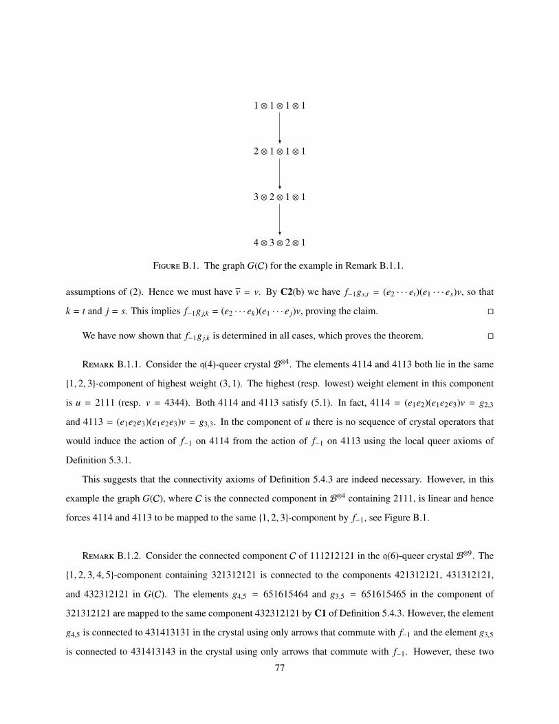
4 ⊗ 3 ⊗ 2 ⊗ 1

3 ⊗ 2 ⊗ 1 ⊗ 1

2 ⊗ 1 ⊗ 1 ⊗ 1

1 ⊗ 1 ⊗ 1 ⊗ 1

Figure B.1. The graph G(C) for the example in Remark B.1.1.

assumptions of (2). Hence we must have v = v. By C2(b) we have f−1gs,t = (e2 · · · et)(e1 · · · es)v, so that

k = t and j = s. This implies f−1g j,k = (e2 · · · ek)(e1 · · · e j)v, proving the claim. �

We have now shown that f−1g j,k is determined in all cases, which proves the theorem. �

Remark B.1.1. Consider the q(4)-queer crystal B⊗4. The elements 4114 and 4113 both lie in the same

{1, 2, 3}-component of highest weight (3, 1). The highest (resp. lowest) weight element in this component

is u = 2111 (resp. v = 4344). Both 4114 and 4113 satisfy (5.1). In fact, 4114 = (e1e2)(e1e2e3)v = g2,3

and 4113 = (e1e2e3)(e1e2e3)v = g3,3. In the component of u there is no sequence of crystal operators that

would induce the action of f−1 on 4114 from the action of f−1 on 4113 using the local queer axioms of

Definition 5.3.1.

This suggests that the connectivity axioms of Definition 5.4.3 are indeed necessary. However, in this

example the graph G(C), where C is the connected component in B⊗4 containing 2111, is linear and hence

forces 4114 and 4113 to be mapped to the same {1, 2, 3}-component by f−1, see Figure B.1.

Remark B.1.2. Consider the connected component C of 111212121 in the q(6)-queer crystal B⊗9. The

{1, 2, 3, 4, 5}-component containing 321312121 is connected to the components 421312121, 431312121,

and 432312121 in G(C). The elements g4,5 = 651615464 and g3,5 = 651615465 in the component of

321312121 are mapped to the same component 432312121 by C1 of Definition 5.4.3. However, the element

g4,5 is connected to 431413131 in the crystal using only arrows that commute with f−1 and the element g3,5

is connected to 431413143 in the crystal using only arrows that commute with f−1. However, these two

77

components (containing 431413131 resp. 431413143 using only crystal operators fi and ei with i ∈ I0 that

commute with f−1) are disjoint. This suggests that C1 of Definition 5.4.3 is necessary for uniqueness.

B.2.

In this appendix we prove Theorem 5.4.5.

We use the shorthand notation ek1 := e1 · · · ek, ek

1:= e−1e2 · · · ek, f 1

k := fk · · · f1, and f 1k := fk · · · f2 f−1.

Lemma B.2.1. In B⊗`, condition C0 of Definition 5.4.3 holds.

Proof. This follows from Remark 5.4.4. �

The connectivity axioms C1 and C2 of Definition 5.4.3 are implied by the following conditions. Here v

is an I0-lowest weight vector in C:

C1’. If h < k and there exists some j ∈ (h, k] such that f 1h f 1

j e j1ek

1(v) is I0-lowest weight, then for any

j′ ∈ (h, k] with e j′

1 ek1(v) , 0 we have f 1

j′ej′

1 ek1(v) = f 1

j e j1ek

1(v).

C2’. If j 6 k and f−1e j1ek

1(v) , 0, then either:

(a) j , k and f 1j f 1

k e j1ek

1(v) = v, or

(b) f 1h f 1

j e j1ek

1(v) is I0-lowest weight for some h < j.

Proposition B.2.2. In B⊗`, condition C2’ holds.

The proof of Proposition B.2.2 is given in Section B.2.1.

Proposition B.2.3. In B⊗`, condition C1’ holds.

We will prove a seemingly weaker statement:

Lemma B.2.4. In B⊗`, condition C1’ holds for j = n − 1, j′ = k = n and for j = k = n, j′ = n − 1.

The proof of Lemma B.2.4 is given in Sections B.2.2 and B.2.3.

Proposition B.2.5. Lemma B.2.4 implies Proposition B.2.3.

78

Proof. We first assume that h < j < j′ 6 k and the assumptions in C1’ hold. Then we have

f 1h f 1

j e j1ek

1(v) = f 1h f 1

j ( f j′ · · · f j+2)(e j+2 · · · e j′)ej1ek

1(v)

= ( f j′ · · · f j+2) f 1h f 1

j e j1(e j+2 · · · e j′)ek

1(v)

= ( f j′ · · · f j+2) f 1h f 1

j e j1e j+1

1 (v′),

where v′ = (e j+2 · · · e j′)(e j+2 · · · ek)(v). Here we have used Stembridge relations to commute crystal oper-

ators and in the last step also that the operators are acting on an I0-lowest weight element. Note that v′ is

{1, . . . , j + 1}-lowest weight. Moreover, f 1h f 1

j e j1e j+1

1 (v′) is {1, . . . , j + 1}-lowest weight. Since e j+11 e j+1

1 (v′) =

e j′

1 ek1(v) , 0, we may apply Lemma B.2.4 with n = j + 1. This implies

( f j′ · · · f j+2) f 1h f 1

j e j1e j+1

1 (v′) = ( f j′ · · · f j+2) f 1h f 1

j+1e j+11 e j+1

1 (v′)

= f 1h f 1

j′ej+11 e j+1

1 (e j+2 · · · e j′)(e j+2 · · · ek)(v)

= f 1h f 1

j′ej′

1 ek1(v),

which proves the claim.

Next assume that h < j′ < j 6 k. Then

f 1h f 1

j e j1ek

1(v) = f 1h f 1

j e j′+11 e j′+1

1 (e j′+2 · · · e j)(e j′+2 · · · ek)(v) = ( f j · · · f j′+2) f 1h f 1

j′+1e j′+11 e j′+1

1 (v′),

where v′ = (e j′+2 · · · e j)(e j′+2 · · · ek)(v). In this case, both v′ and f 1h f 1

j′+1e j′+11 e j′+1

1 (v′) are {1, . . . , j′+1}-lowest

weight. Since e j′

1 e j′+11 (v′) , 0, we may apply Lemma B.2.4 with n = j′ + 1 to obtain

f 1h f 1

j e j1ek

1(v) = ( f j · · · f j′+2) f 1h f 1

j′ej′

1 e j′+11 (v′) = f 1

h f 1j′e

j′

1 ek1(v),

proving the claim. �

B.2.1. Proof of Proposition B.2.2. Given a word w = w1 · · ·w` in the letters {1, . . . , n + 1} we write

w# = w` · · ·w1, where wi = n + 2 − wi. Suppose that x = g j,k = e j1ek

1(v) ∈ B⊗`, where v is I0-lowest weight

and 1 6 j 6 k 6 n, so that by Lemma 5.3.3 we have ϕ1(x) = 2 and ϕi(x) = 0 for all i > 1. The RSK insertion

tableau for x#, denoted by P(x#), can be constructed as follows: Construct the semistandard Young tableau

with weight and shape equal to the weight of v#. Change the rightmost n + 1 − k in row n + 1 − k and the

rightmost n + 1 − j in row n + 1 − j to n + 1.

79

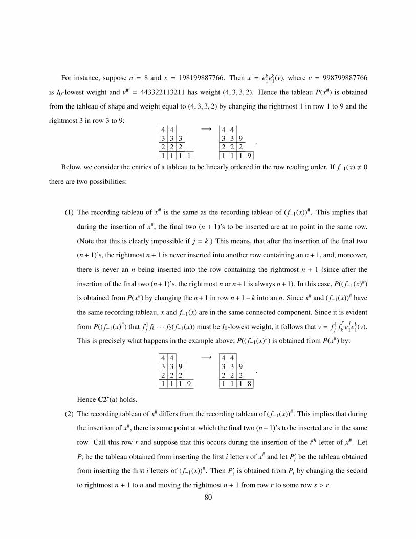
For instance, suppose n = 8 and x = 198199887766. Then x = e61e8

1(v), where v = 998799887766

is I0-lowest weight and v# = 443322113211 has weight (4, 3, 3, 2). Hence the tableau P(x#) is obtained

from the tableau of shape and weight equal to (4, 3, 3, 2) by changing the rightmost 1 in row 1 to 9 and the

rightmost 3 in row 3 to 9:4 43 3 32 2 21 1 1 1

−→ 4 43 3 92 2 21 1 1 9

.

Below, we consider the entries of a tableau to be linearly ordered in the row reading order. If f−1(x) , 0

there are two possibilities:

(1) The recording tableau of x# is the same as the recording tableau of ( f−1(x))#. This implies that

during the insertion of x#, the final two (n + 1)’s to be inserted are at no point in the same row.

(Note that this is clearly impossible if j = k.) This means, that after the insertion of the final two

(n + 1)’s, the rightmost n + 1 is never inserted into another row containing an n + 1, and, moreover,

there is never an n being inserted into the row containing the rightmost n + 1 (since after the

insertion of the final two (n+1)’s, the rightmost n or n+1 is always n+1). In this case, P(( f−1(x)#)

is obtained from P(x#) by changing the n + 1 in row n + 1− k into an n. Since x# and ( f−1(x))# have

the same recording tableau, x and f−1(x) are in the same connected component. Since it is evident

from P(( f−1(x)#) that f 1j fk · · · f2( f−1(x)) must be I0-lowest weight, it follows that v = f 1

j f 1k e j

1ek1(v).

This is precisely what happens in the example above; P(( f−1(x)#) is obtained from P(x#) by:

4 43 3 92 2 21 1 1 9

−→ 4 43 3 92 2 21 1 1 8

.

Hence C2’(a) holds.

(2) The recording tableau of x# differs from the recording tableau of ( f−1(x))#. This implies that during

the insertion of x#, there is some point at which the final two (n + 1)’s to be inserted are in the same

row. Call this row r and suppose that this occurs during the insertion of the ith letter of x#. Let

Pi be the tableau obtained from inserting the first i letters of x# and let P′i be the tableau obtained

from inserting the first i letters of ( f−1(x))#. Then P′i is obtained from Pi by changing the second

to rightmost n + 1 to n and moving the rightmost n + 1 from row r to some row s > r.

80

Now continue with the insertion of the (i + 1)st letter in each case. Since the (n, n + 1)-subword

of x# ends with two (n+1)’s, and these are the only (n, n+1)-unbracketed (n+1)’s in this subword,

the same is true of the (n, n+1)-subword of each of Pi, Pi+1, . . . , P`. This implies that at no point in

the rest of the insertion of x# is the second to rightmost n + 1 inserted into a row containing another

n + 1, and moreover at no point is an n inserted into the row containing the second to rightmost

n + 1 (since after the insertion of the final two (n + 1)’s, the two rightmost entries which are either

n or n + 1 must both be n + 1).

It follows that, if we ignore, the rightmost n + 1 in P(( f−1(x)#) and P(x#), then they have the

same shape, and the second differs from the first only by changing its rightmost n to n + 1. Adding

back the rightmost n + 1 to P(x#), we see that it must go somewhere to the right of this position (by

definition), and adding back the rightmost n + 1 to P( f−1(x#)), we see that it must go somewhere

to the left of this position (otherwise P(( f−1(x)#) would have an (n, n + 1)-unbracketed n + 1.)

It follows that P(( f−1(x)#) is obtained from P(x#) by eliminating the (rightmost) n + 1 in row

n − k + 1, changing the (leftmost) n + 1 in row n − j + 1 to n and adding an n + 1 to some row

n − h + 1 for h < j. It follows that v′ = f 1h f 1

j e j1ek

1(v) and v are both (distinct) I0-lowest weight

elements. Hence C2’(b) holds.

To see an example of the second case, let v = 99889. Then v# = 12211, (e71e8

1(v))# = 29911,

( f−1e71e8

1(v))# = 29811, and ( f 16 f 1

7 e71e8

1(v))# = 23211 have the following insertion tableaux:

2 21 1 1

−→ 2 91 1 9

−→ 92 81 1

−→ 32 21 1

.

B.2.2. Proof of Lemma B.2.4 for j = n − 1 and j′ = n. Define X = (e1 · · · en)v. For 1 6 i 6 n + 1,

set Ai = (ei · · · en)X and Bi = (ei · · · en−1)X. For 2 6 i 6 n + 1, set A−i = ( f(i−1) · · · f2 f−1)A1 and B−i =

( f(i−1) · · · f2 f−1)B1. (So A1 = A−1 and B1 = B−1. Moreover, Bn+1 = Bn.) By assumption ( fh · · · f1)(B−n) is

I0-lowest weight, so fn( fh · · · f1)(B−n) = 0 and hence B−(n+1) = 0.

Let xi be the integer which represents the position where Ai+1 and Ai differ, and yi be the integer which

represents the position where Bi+1 and Bi differ. Also, let x−i be the integer which represents the position

where A−i and A−(i+1) differ, and let y−i be the integer which represents the position where B−i and B−(i+1)

differ. Note that yn and y−n are undefined.

81

Recall that v ∈ B⊗`. Suppose W is any word of length ` in the letters {1, . . . , n + 1}. If 1 6 p 6 `, we

define W(p) to be the pth entry of W. If 1 6 p 6 q 6 ` are integers, then the notation W(p : q) will be used

to refer to the word W(p)W(p + 1) . . .W(q − 1)W(q).

If 1 6 i 6 n, we define the i/(i + 1)-subword of W to be the word composed of the symbols {i, i + 1, }

which is obtained from W by changing each entry that is neither i nor i + 1 to the symbol . For instance the

2/3-subword of 241432143 is 2 32 3. When we speak of erasing an i or i + 1, we mean changing that

entry to ; similarly, when we speak of adding an i or i + 1, we mean changing some to i or i + 1. Moving

an i or i + 1 from p to q means erasing an i or i + 1 from position p and adding an i or i + 1 to position q. The

notation W(p : q) is used in the same way for subwords as it is for words. For instance, if W=3 32 3

then W(3 : 7) = 32 .

Claim B.2.6. For 2 6 i 6 n, we have xi > xi−1. For 2 6 i 6 n − 1, we have yi > yi−1.

Proof. If xi < xi−1, then it follows that fiAi−1 , 0. But this is the statement that

fi(ei−1ei · · · en)(e1 · · · en)v , 0

for some integer 2 6 i 6 n, which is absurd since v is I0-lowest weight. If yi < yi−1, then it follows that

fiBi−1 , 0. But this is the statement that

fi(ei−1ei · · · en−1)(e1 · · · en)v , 0

for some integer 2 6 i 6 n − 1, which is also absurd. �

Claim B.2.7. We have x1 > x−1 and y1 > y−1. (In particular, f−1(A1) , 0, so x−1 is well-defined.)

Proof. By the definition of the operator f−1 we have y1 > y−1. Since v and v∗ := f 1h f 1

n−1en−11 en

1v

are both I0-lowest weight and have different weights, we cannot have y1 = y−1. Thus y1 > y−1. Now

Bn(1 : y−1) = B1(1 : y−1). Therefore, there are no 1’s or 2’s in Bn(1 : y−1 − 1) and we have Bn(y−1) = 1

since these statements must be true of B1. If x1 > y−1, then A1(1 : y−1) = B1(1 : y−1) and so A−2 , 0

with x−1 = y−1. If x1 < y−1, then A1(1 : x1 − 1) = Bn(1 : x1 − 1) contains no 1’s or 2’s and A1(x1) = 1.

Thus A−2 , 0 with x−1 = x1. It is clearly impossible for x1 = y−1. Therefore, we have established that

A−2 = f−1(A1) , 0. In the notation of Proposition B.2.2, we have for j = k = n, that f−1e j1ek

1(v) , 0. Hence

82

we must be in case C2’(b) from which we deduce that f−1(A1) lies in a different I0-connected component

than A1. From this it follows that x1 > x−1. �

Claim B.2.8. For 2 6 i 6 n, we have x−(i−1) 6 x−i. For 2 6 i 6 n, we have y−(i−1) 6 y−i. (In particular,

A−3, . . . , A−(n+1) are nonzero, so x−2, . . . , x−n are well-defined.)

Proof. Again, case C2’(b) applies to f−1(A1) and so the parenthetical statement is immediate. First, it

is clear from the definitions of the f−1 and f2 operators that x−1 6 x−2 and that y−1 6 y−2. If x−(i−1) > x−i for

i > 2, then it follows that fiA−(i−1) , 0. But this is the statement that fi(ei−1ei · · · en)(e1 · · · eg)v , 0 for some

I0-lowest weight element v and integers 3 6 i 6 n and 0 6 g < n which is absurd. If y−(i−1) > y−i for i > 2,

then it follows that fi(B−(i−1)) , 0. But this is the statement that fi(ei−1ei · · · en−1)(e1 · · · eg)v∗ , 0 for some

integers 3 6 i 6 n and 0 6 g < n which is equally absurd. �

So far, we have the following situation:

xn > · · · > x2 > x1 > x−1 6 x−2 6 · · · 6 x−n and

yn−1 > · · · > y2 > y1 > y−1 6 y−2 6 · · · 6 y−(n−1).

Claim B.2.9. We have x−1 = y−1.

Proof. Since x1 = y−1 is impossible and since x1 < y−1 would imply that x−1 = x1, which contradicts

x1 > x−1, we may assume x1 > y−1. However, in this case we have A1(1 : y−1) = B1(1 : y−1). Since f−1 acts

on B1 in position y−1, it follows that f−1 acts on A1 in position y−1 as well. This implies x−1 = y−1. �

Claim B.2.10. For 1 6 i 6 n − 1, we have xi 6 yi.

Proof. First we show that xn−1 6 yn−1. Now yn−1 represents the position of the leftmost (n − 1, n)-

unbracketed n in Bn. This n is also unbracketed in An because the (n − 1)/n-subword of An is obtained

from the (n − 1)/n-subword of Bn by inserting an n. Hence the leftmost (n − 1, n)-unbracketed n in An is

weakly to the left of position yn−1, so xn−1 6 yn−1. Next, suppose that xi+1 6 yi+1 but xi > yi. The i/(i + 1)-

subword of Ai+1 only differs from the i/(i + 1)-subword of Bi+1 by moving an i + 1 to the left from yi+1

to xi+1. Since yi < xi+1 by assumption, the i + 1 which appears in Bi+1(yi) still appears in Ai+1(yi) and is

(i, i + 1)-unbracketed. This implies xi 6 yi. Induction completes the proof. �

Claim B.2.11. For 1 6 i 6 n, we have xi > x−i. For 1 6 i 6 n − 1, we have yi > y−i.

83

Proof. We already know that x1 > x−1. So assume that xi−1 > x−(i−1) but xi < x−i. The i/(i+1)-subword

of Ai is obtained from the i/(i + 1)-subword of A−i by moving an i to the right from x−(i−1) to xi−1. Since

A−i(x−i) contains an (i, i + 1)-unbracketed i and xi−1 < x−i, we see that Ai(x−i) still contains an (i, i + 1)-

unbracketed i. This implies that xi > x−i. Induction completes the proof. The second statement is proved in

the same way. �

From the previous result, we have the following situation:

· · · > x3 > x2 > x1 > x−1 6 x−2 6 x−3 6 · · ·

6 6 6

||

· · · > y3 > y2 > y1 > y−1 6 y−2 6 y−3 6 · · ·

where every entry on the left side of the array is > to its mirror image on the right side of the array. From

now on, let j be minimal such that x j < y j; if no such j exists, set j = n.

Claim B.2.12. We have xi = yi for all i < j and xi+1 < yi for all j 6 i < n.

Proof. The first claim is immediate. Next we note that xi < yi for all i > j. (Otherwise xi = yi for

some i > j. This implies that xk = yk for all k 6 i, and, in particular, x j = y j.) By definition, we have

Bi+1(yi) = i + 1 and Ai+2(xi+1) = i + 2. From the latter, it follows that Bi+2(xi+1) > i + 2 and, since yi+1 > xi+1

(or yi+1 is undefined) that Bi+1(xi+1) > i + 2. Therefore, we have xi+1 , yi. If xi+1 > yi, we must have

xi < xi+1 and yi < yi+1 from which it follows that Ai+1(1 : yi) = Bi+1(1 : yi). But this makes xi < yi

impossible. By contradiction, we conclude that xi+1 < yi. �

Claim B.2.13. For i < j we have x−i = y−i. Also, x j > x j−1.

Proof. Since the restrictions of A j−1 and B j−1 to the alphabet {1, 2, . . . , j−1} are identical, and since the

operators e j−2, . . . , e1, f−1, f2, . . . , f j−2 only depend on and effect these letters, it follows that for i 6 j−2 we

have x−i = y−i. Now we must show x−( j−1) = y−( j−1). We have A j+1(x j) = j + 1 and thus B j+1(x j) > j + 1,

and hence by x j < y j, B j(x j) > j + 1. Since B j(y j−1) = j, this yields x j , y j−1. In light of x j−1 = y j−1 this

gives x j , x j−1. From this it follows that A j(1 : x j−1) = B j(1 : x j−1). By the minimality of j and by the

result for i 6 j − 2 this implies that A−( j−1)(1 : x j−1) = B−( j−1)(1 : x j−1). Since we have both x−( j−1) 6 x j−1

and y−( j−1) 6 y j−1, the previous equality implies that x−( j−1) = y−( j−1). �

84

If 1 < i < n, let #(A−i(p : q)) denote the number of i’s minus the number of (i + 1)’s which appear in

A−i(p : q). Define #(B−i(p : q)) analogously. Set ABi(p : q) = #(A−i(p : q)) − #(B−i(p : q)).

Claim B.2.14. Suppose 1 < i < n.

(1) If x−i < y−i, then ABi(1 : x−i) > 0.

(2) If x−i > y−i, then ABi(1 : y−i) < 0.

(3) If x−i < y−i, then ABi(x−i + 1 : y−i) < 0.

(4) If x−i < y−i, x−i = xi, xi , xi+1, and xi , yi, then ABi(x−i + 1 : yi) < −1.

Proof. Once again, C2’(b) applies to f−1(A1) and so we may write A−i = ei · · · eneh′1 (v′) for some I0-

lowest weight element v′ and some h′ < n. It follows that A−i has exactly one (i, i + 1)-unbracketed i and

it occurs in x−i. In addition, case C2’(b) applies to f−1(B1) by assumption, so B−i = ei · · · en−1eh1(v∗) for an

I0-lowest weight element v∗. Hence B−i has exactly one (i, i + 1)-unbracketed i and it occurs in y−i. Thus

we have #(A−i(1 : x−i)) > 0 and #(B−i(1 : y−i)) > 0. If x−i < y−i then #(B−i(1 : x−i)) 6 0, while if

x−i > y−i then #(A−i(1 : y−i)) 6 0. Together this proves the first two statements. For the third statement

we have #(A−i(x−i + 1 : y−i)) 6 0 and #(B−i(x−i + 1 : y−i)) > 0. For the fourth statement, again, we have

#(A−i(x−i + 1 : y−i)) 6 0, but now note that Ai+1(xi) = i + 1. Since xi , xi+1, also, Ai+2(xi) = i + 1, whence

Bi+1(xi) = i+1, and, by, xi , yi, we have Bi(xi) = i+1. This now implies that B−i(xi) = i+1 or B−i(x−i) = i+1.

Since the i in B−i(yi) must be (i, i + 1)-unbracketed this implies that #(B−i(x−i + 1 : y−i)) > 1. �

Claim B.2.15. Fix an interval [p, q]. We define the function [t] by [t] = 1 if t ∈ [p, q] and [t] = 0

otherwise. With this notation, we have that

ABi(p : q) = [x−(i−1)] − [xi−1] + 2[xi] − [xi+1] + [yi+1] − 2[yi] + [yi−1] − [y−(i−1)].

Proof. This is a straightforward computation. �

Claim B.2.16. Suppose j < n. If either x j > x− j or y j > y− j, then both x j > x− j and y j > y− j. In this

case we have x− j = y− j.

Proof. If j = 1, the conclusions of the claim have already been proven in previous claims. Thus assume

j > 1. First note that, since x−( j−1) = y−( j−1) and x j−1 = y j−1, we have AB j(p : q) = 2[x j] − [x j+1] + [y j+1] −

85

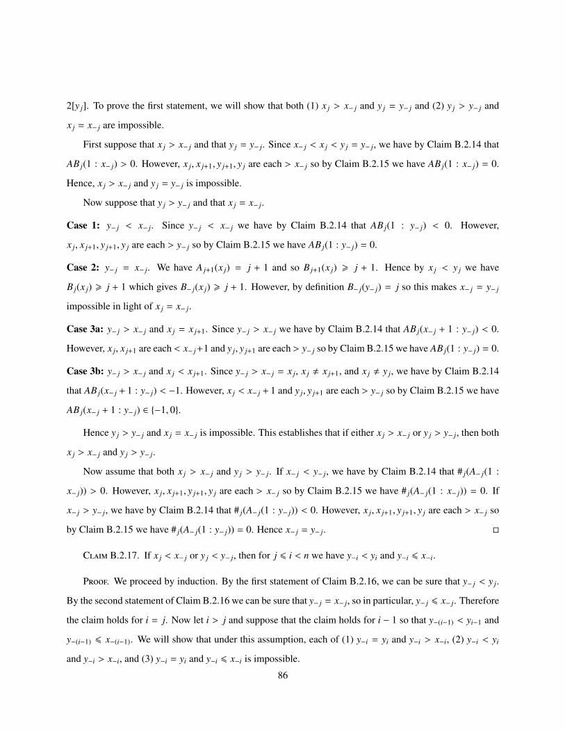
2[y j]. To prove the first statement, we will show that both (1) x j > x− j and y j = y− j and (2) y j > y− j and

x j = x− j are impossible.

First suppose that x j > x− j and that y j = y− j. Since x− j < x j < y j = y− j, we have by Claim B.2.14 that

AB j(1 : x− j) > 0. However, x j, x j+1, y j+1, y j are each > x− j so by Claim B.2.15 we have AB j(1 : x− j) = 0.

Hence, x j > x− j and y j = y− j is impossible.

Now suppose that y j > y− j and that x j = x− j.

Case 1: y− j < x− j. Since y− j < x− j we have by Claim B.2.14 that AB j(1 : y− j) < 0. However,

x j, x j+1, y j+1, y j are each > y− j so by Claim B.2.15 we have AB j(1 : y− j) = 0.

Case 2: y− j = x− j. We have A j+1(x j) = j + 1 and so B j+1(x j) > j + 1. Hence by x j < y j we have

B j(x j) > j + 1 which gives B− j(x j) > j + 1. However, by definition B− j(y− j) = j so this makes x− j = y− j

impossible in light of x j = x− j.

Case 3a: y− j > x− j and x j = x j+1. Since y− j > x− j we have by Claim B.2.14 that AB j(x− j + 1 : y− j) < 0.

However, x j, x j+1 are each < x− j+1 and y j, y j+1 are each > y− j so by Claim B.2.15 we have AB j(1 : y− j) = 0.

Case 3b: y− j > x− j and x j < x j+1. Since y− j > x− j = x j, x j , x j+1, and x j , y j, we have by Claim B.2.14

that AB j(x− j + 1 : y− j) < −1. However, x j < x− j + 1 and y j, y j+1 are each > y− j so by Claim B.2.15 we have

AB j(x− j + 1 : y− j) ∈ {−1, 0}.

Hence y j > y− j and x j = x− j is impossible. This establishes that if either x j > x− j or y j > y− j, then both

x j > x− j and y j > y− j.

Now assume that both x j > x− j and y j > y− j. If x− j < y− j, we have by Claim B.2.14 that # j(A− j(1 :

x− j)) > 0. However, x j, x j+1, y j+1, y j are each > x− j so by Claim B.2.15 we have # j(A− j(1 : x− j)) = 0. If

x− j > y− j, we have by Claim B.2.14 that # j(A− j(1 : y− j)) < 0. However, x j, x j+1, y j+1, y j are each > x− j so

by Claim B.2.15 we have # j(A− j(1 : y− j)) = 0. Hence x− j = y− j. �

Claim B.2.17. If x j < x− j or y j < y− j, then for j 6 i < n we have y−i < yi and y−i 6 x−i.

Proof. We proceed by induction. By the first statement of Claim B.2.16, we can be sure that y− j < y j.

By the second statement of Claim B.2.16 we can be sure that y− j = x− j, so in particular, y− j 6 x− j. Therefore

the claim holds for i = j. Now let i > j and suppose that the claim holds for i − 1 so that y−(i−1) < yi−1 and

y−(i−1) 6 x−(i−1). We will show that under this assumption, each of (1) y−i = yi and y−i > x−i, (2) y−i < yi

and y−i > x−i, and (3) y−i = yi and y−i 6 x−i is impossible.

86

First suppose that y−i = yi and that y−i > x−i.

Case 1: x−i < xi. Since y−i > x−i by Claim B.2.14 we have ABi(1 : x−i) > 0. However, by assumption

xi, xi+1, yi+1, yi, yi−1 are each > x−i and x−(i−1) = y−(i−1) so the only possible relevant change is at xi−1. Thus

by Claim B.2.15 we have ABi(1 : y−i) ∈ {−1, 0}.

Case 2a: x−i = xi and xi = xi+1. Since y−i > x−i by Claim B.2.14 we have ABi(1 : x−i) > 0. By assumptions,

each of x−(i−1), xi−1, xi, xi+1, y−(i−1) are < x−i + 1. Clearly yi = y−i ∈ [x−i + 1 : y−i]. Moreover, yi−1 6 yi = y−i

and yi−1 > xi = x−i, so yi−1 ∈ [x−i + 1 : y−i]. Without computing the value of [yi+1] we may conclude by

Claim B.2.15 that ABi(1 : y− j) ∈ {−1, 0}.

Case 2b: x−i = xi and xi < xi+1. Since y−i > x−i, x−i = xi, xi , xi+1, and xi , yi we have by Claim B.2.14

that ABi(x−i + 1 : y−i) < −1. By assumptions, each of x−(i−1), xi−1, xi, y−(i−1) are < x−i + 1. Again, we

know that yi, yi−1 ∈ [x−i + 1 : y−i]. Without computing the value of [yi+1] and [xi+1] we may compute by

Claim B.2.15 that ABi(x−i + 1 : y−i) ∈ {−1, 0, 1}.

Hence it is impossible that y−i = yi and that y−i > x−i. Now suppose that y−i < yi and that y−i > x−i.

Case 1a: x−i < xi and xi 6 y−i. Since y−i > x−i, we have by Claim B.2.14 that ABi(x−i + 1 : y−i) < 0. We

have that x−(i−1), y−(i−1) are both < x−i + 1, that xi ∈ [x−i + 1 : y−i] and that yi, yi+1 are both > y−i. Without

computing [xi−1], [xi+1], [yi−1] we may determine by Claim B.2.15 that ABi(x−i + 1 : y−i) ∈ {0, 1, 2, 3}.

Case 1bi: x−i < xi, xi > y−i, and xi−1 6 x−i. Since y−i > x−i, we have by Claim B.2.14 that ABi(x−i + 1 :

y−i) < 0. By assumption each of x−(i−1), xi−1, y−(i−1) are < x−i + 1 and xi+1, xi, yi, yi+1 are > y−i. Without

computing [yi−1] we may determine by Claim B.2.15 that ABi(x−i + 1 : y−i) ∈ {0, 1}.

Case 1bii: x−i < xi, xi > y−i, and xi−1 > x−i. Since y−i > x−i, we have by Claim B.2.14 that ABi(1 :

x−i) < 0. By assumption x−(i−1), y−(i−1) are 6 x−i whereas each of xi−1, xi, xi+1, yi−1, yi, yi+1 are > x−i. Thus

by Claim B.2.15, we have ABi(1 : x−i) = 0.

Case 2a: x−i = xi and xi = xi+1. Since y−i > x−i we have by Claim B.2.14 that ABi(x−i + 1 : y−i) < 0. By

assumption each of x−(i−1), xi−1, xi, xi+1, y−(i−1) are < x−i + 1 and yi, yi+1 are > y−i. Without computing [yi−1]

we may determine by Claim B.2.15 that ABi(x−i + 1 : y−i) ∈ {0, 1}.

87

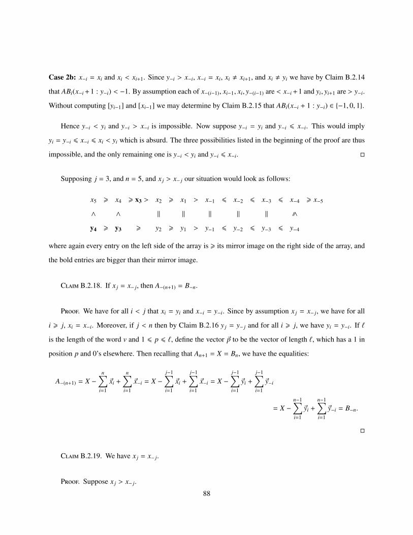
Case 2b: x−i = xi and xi < xi+1. Since y−i > x−i, x−i = xi, xi , xi+1, and xi , yi we have by Claim B.2.14

that ABi(x−i +1 : y−i) < −1. By assumption each of x−(i−1), xi−1, xi, y−(i−1) are < x−i +1 and yi, yi+1 are > y−i.

Without computing [yi−1] and [xi−1] we may determine by Claim B.2.15 that ABi(x−i + 1 : y−i) ∈ {−1, 0, 1}.

Hence y−i < yi and y−i > x−i is impossible. Now suppose y−i = yi and y−i 6 x−i. This would imply

yi = y−i 6 x−i 6 xi < yi which is absurd. The three possibilities listed in the beginning of the proof are thus

impossible, and the only remaining one is y−i < yi and y−i 6 x−i. �

Supposing j = 3, and n = 5, and x j > x− j our situation would look as follows:

x5 > x4 > x3 > x2 > x1 > x−1 6 x−2 6 x−3 6 x−4 > x−5

∧ ∧ || || || || ||

6

y4 > y3 > y2 > y1 > y−1 6 y−2 6 y−3 6 y−4

where again every entry on the left side of the array is > its mirror image on the right side of the array, and

the bold entries are bigger than their mirror image.

Claim B.2.18. If x j = x− j, then A−(n+1) = B−n.

Proof. We have for all i < j that xi = yi and x−i = y−i. Since by assumption x j = x− j, we have for all

i > j, xi = x−i. Moreover, if j < n then by Claim B.2.16 y j = y− j and for all i > j, we have yi = y−i. If `

is the length of the word v and 1 6 p 6 `, define the vector ~p to be the vector of length `, which has a 1 in

position p and 0’s elsewhere. Then recalling that An+1 = X = Bn, we have the equalities:

A−(n+1) = X −n∑

i=1

~xi +

n∑i=1

~x−i = X −j−1∑i=1

~xi +

j−1∑i=1

~x−i = X −j−1∑i=1

~yi +

j−1∑i=1

~y−i

= X −n−1∑i=1

~yi +

n−1∑i=1

~y−i = B−n.

�

Claim B.2.19. We have x j = x− j.

Proof. Suppose x j > x− j.

88

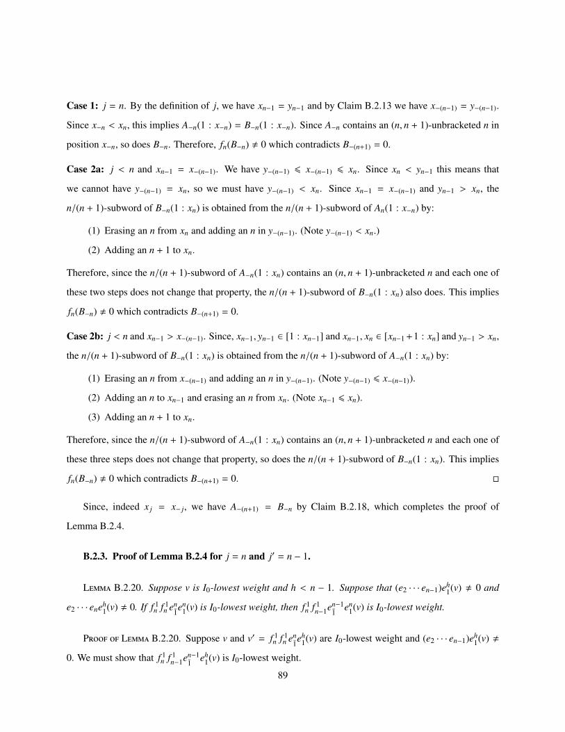
Case 1: j = n. By the definition of j, we have xn−1 = yn−1 and by Claim B.2.13 we have x−(n−1) = y−(n−1).

Since x−n < xn, this implies A−n(1 : x−n) = B−n(1 : x−n). Since A−n contains an (n, n + 1)-unbracketed n in

position x−n, so does B−n. Therefore, fn(B−n) , 0 which contradicts B−(n+1) = 0.

Case 2a: j < n and xn−1 = x−(n−1). We have y−(n−1) 6 x−(n−1) 6 xn. Since xn < yn−1 this means that

we cannot have y−(n−1) = xn, so we must have y−(n−1) < xn. Since xn−1 = x−(n−1) and yn−1 > xn, the

n/(n + 1)-subword of B−n(1 : xn) is obtained from the n/(n + 1)-subword of An(1 : x−n) by:

(1) Erasing an n from xn and adding an n in y−(n−1). (Note y−(n−1) < xn.)

(2) Adding an n + 1 to xn.

Therefore, since the n/(n + 1)-subword of A−n(1 : xn) contains an (n, n + 1)-unbracketed n and each one of

these two steps does not change that property, the n/(n + 1)-subword of B−n(1 : xn) also does. This implies

fn(B−n) , 0 which contradicts B−(n+1) = 0.

Case 2b: j < n and xn−1 > x−(n−1). Since, xn−1, yn−1 ∈ [1 : xn−1] and xn−1, xn ∈ [xn−1 +1 : xn] and yn−1 > xn,

the n/(n + 1)-subword of B−n(1 : xn) is obtained from the n/(n + 1)-subword of A−n(1 : xn) by:

(1) Erasing an n from x−(n−1) and adding an n in y−(n−1). (Note y−(n−1) 6 x−(n−1)).

(2) Adding an n to xn−1 and erasing an n from xn. (Note xn−1 6 xn).

(3) Adding an n + 1 to xn.

Therefore, since the n/(n + 1)-subword of A−n(1 : xn) contains an (n, n + 1)-unbracketed n and each one of

these three steps does not change that property, so does the n/(n + 1)-subword of B−n(1 : xn). This implies

fn(B−n) , 0 which contradicts B−(n+1) = 0. �

Since, indeed x j = x− j, we have A−(n+1) = B−n by Claim B.2.18, which completes the proof of

Lemma B.2.4.

B.2.3. Proof of Lemma B.2.4 for j = n and j′ = n − 1.

Lemma B.2.20. Suppose v is I0-lowest weight and h < n − 1. Suppose that (e2 · · · en−1)eh1(v) , 0 and

e2 · · · eneh1(v) , 0. If f 1

n f 1n en

1en

1(v) is I0-lowest weight, then f 1n f 1

n−1en−11

en1(v) is I0-lowest weight.

Proof of Lemma B.2.20. Suppose v and v′ = f 1n f 1

n en1eh

1(v) are I0-lowest weight and (e2 · · · en−1)eh1(v) ,

0. We must show that f 1n f 1

n−1en−11

eh1(v) is I0-lowest weight.

89

Claim B.2.21. Given a word W, define L(W) to be the length of the longest weakly increasing subse-

quence of W. If V is I0-lowest weight, and W and V are in the same I0-connected component, then the

number of (n + 1)’s which appear in V is equal to L(W).

Proof. This easily follows from analyzing the RSK insertion tableaux of the words. �

Claim B.2.22. We have L(en−11

eh1(v)) > L(en

1eh

1(v)).

Proof. Since Y = e2 · · · en−1eh1(v) , 0, by inspection of the insertion tableaux of v and Y we observe that

ϕ1(Y) = 0, ϕ2(Y) = 1, and ϕk(Y) = 0 for all k > 2. This implies that Y contains a letter 2 which precedes all

letters 1. Hence en−11

eh1(v) = e−1(Y) , 0, so the statement L(en−1

1eh

1(v)) > L(en1eh

1(v)) is well-defined.

We will now recycle notation from the proof of Section B.2.2 with slight changes. Let X = eh1(v). For

2 6 i 6 n + 1, set Ai = (ei · · · en)(X) and Bi = (ei · · · en−1)(X). Set A1 = e−1(A2) and B1 = e−1(B2). Let xi be

the integer which represents the position, where Ai+1 and Ai differ and yi be the integer which represents the

position where Bi+1 and Bi differ.

Suppose that v contains r letters (n + 1). It follows from weight considerations that v′ contains (r + 1)

letters (n + 1). This implies that L(en1eh

1(v)) = r + 1 whereas L(e2 · · · eneh1(v)) = r. This is to say L(A1) = r + 1

and L(A2) = r. So A1 contains a weakly increasing subsequence of length r + 1, specified by the indices

i01, . . . , ir1. We must have that i01 = x1 and that A1(i11) = 1, otherwise the same indices would specify a

weakly increasing subsequence of A2 of length r +1. It follows that A2 has a weakly increasing subsequence

given by the indices i12, . . . , ir2 where A2(i12) = 1. Now suppose 2 6 k 6 n and Ak has a weakly increasing

subsequence given by the indices i1k , . . . , irk, where Ak(i1k) = 1. If xk < {i1k , . . . , i

rk}, then Ak+1 has such a

subsequence specified by the same indices.

Now suppose that xk ∈ {i1k , . . . , irk}. Create a list of indices as follows:

(1) If i jk 6 xk or Ak(i j

k) , k, then i jk+1 = i j

k.

(2) If i jk > xk and Ak(i j

k) = k, then Ak(i jk) is (k, k + 1)-bracketed with some k + 1 in a position between

xk and i jk. Let i j

k+1 denote this position.

This creates a set {i1k+1, . . . , irk+1}, which, after a possible reordering into increasing order, specifies a

weakly increasing subsequence of Ak+1 with Ak+1(i1k+1) = 1.

By induction Bn = An+1 = X has a weakly increasing subsequence specified by the indices {i′1n, . . . , i′rn},

with Bn(i′1n) = 1. Let k > 1 and assume Bk+1 has a weakly increasing subsequence specified by the indices

90

{i′1k+1, . . . , i′rk+1}, with Bk+1(i′1k+1) = 1. If yk < i′1k+1, then the same is true of Bk with the same indices. If

yk > i′1k+1 then Bk = ek(Bk+1) = [Bk+1(1 : i′1k+1) ek(Bk+1(i′1k+1 + 1 : `))]. Since Bk+1(i′1k+1 + 1 : `) has a

weakly increasing subsequence of length r − 1, ek(Bk+1(i′1k+1 + 1 : `)) does as well. Thus Bk = [Bk+1(1 :

i′1k+1) ek(Bk+1(i′1k+1 + 1 : `))] has a weakly increasing subsequence of length r specified by some indices

{i′1k , . . . , i′rk}, with Bk(i′1k) = 1 (where i′1k = i′1k+1). By induction this is true for k = 2. Since e−1(B2) = B1

is defined and since B2(i′12) = 1, we have y1 < i′12 and so {y1, i′12, . . . , i′r2} is a list of indices which give a

weakly increasing subsequence of length r + 1 in B1. �

We want to show that f 1n f 1

n−1en−11

eh1(v) is I0-lowest weight. Now e−1(Y) is obtained from Y = e2 · · · en−1eh

1(v)

by changing its first 2 to 1. As a result ϕ1(e−1(Y)) ∈ {1, 2} and ϕk(e−1(Y)) = 0 for all k > 1. Therefore,

we may write e−1(Y) = es1et

1(v∗) for some I0-lowest weight element v∗, and s > 0 and t > 0 with t > s

(using Lemma 5.3.3 when ϕ1(e−1(Y)) = 2). This gives v∗ = f 1t f 1

s en−11

eh1(v). Since v′ contains one more

n + 1 than v, it follows from Claims B.2.21 and B.2.22 that v∗ contains at least one more n + 1 than v, which

means we must have t = n. This also means that v and v∗ are not in the same connected I0-component. But

if v = f 1h f 1

n−1es1en

1(v∗) is in a different connected I0-component than v∗, then C2’(b) applies which forces

s = n − 1. Thus v∗ = f 1n f 1

n−1en−11

eh1(v).

This concludes the proof of Lemma B.2.20. �

Proposition B.2.23. Lemma B.2.4 with j = n − 1 and j′ = n and Lemma B.2.20 imply Lemma B.2.4.

Proof. We need to show that if v is I0-lowest weight, en−11 en

1(v) , 0, en1en

1(v) , 0, and v∗ = f 1h f 1

n en1en

1(v) is

I0-lowest weight, then f 1n−1en−1

1 en1(v) = f 1

n en1en

1(v). Now v = f 1n f 1

n en1eh

1(v∗) is I0-lowest weight (in particular,

e2 · · · eneh1(v∗) , 0). Now we show that e2 · · · en−1eh

1(v∗) , 0. By definition, eh1(v∗) , 0. Either v∗ has

more n’s than (n − 1)’s so that e2 · · · en−1eh1(v∗) , 0, or else v∗ has the same number of n’s as (n − 1)’s and

h = n − 2 in which case also e2 · · · en−1eh1(v∗) , 0. Therefore, by Lemma B.2.20 v′ = f 1

n f 1n−1en−1

1eh

1(v∗) is

I0-lowest weight. Rewriting this as v∗ = f 1h f 1

n−1en−11 en

1(v′) and noting that wt(v) = wt(v′) implies en1en

1(v′) , 0

Lemma B.2.4 with j = n− 1 and j′ = n gives v∗ = f 1h f 1

n en1en

1(v′). This implies that v = v′ and that hence that

f 1n−1en−1

1 en1(v) = f 1

n en1en

1(v). �

91

Bibliography

[AKO18a] S. Assaf and E. Kantarci Oguz, Crystal graphs for shifted tableaux, Sem. Lothar. Combin. 80B (2018), Art. 26, 12.

[AKO18b] , A local characterization of crystals for the quantum queer superalgebra, (2018), preprint

arXiv:1803.06317v1.

[AS12] F. Ardilla and L. Serrano, Staircase skew Schur functions are Schur P-positive, J. Algebraic Combin. 36 (2012), no. 3,

409–423.

[BH95] S. Billey and M. Haiman, Schubert polynomials for the classical groups, J. Amer. Math. Soc. 8 (1995), no. 2, 443–482.

[BHRY14] S. Billey, Z. Hamaker, A. Roberts, and B. Young, Coxeter-Knuth graphs and a signed Little map for type B reduced

words, Electron. J. Combin. 21 (2014), no. 4, Paper 4.6, 39.

[BS17] D. Bump and A. Schilling, Crystal Bases: Representations and Combinatorics, World Scientific, 2017.

[Cho13] S. Cho, A new Littlewood-Richardson rule for Schur P-functions, Trans. Amer. Math. Soc. 365 (2013), no. 2, 939–972.

[EG87] P. Edelman and C. Greene, Balanced tableaux, Adv. in Math. 63 (1987), no. 1, 42–99.

[FK96] S. Fomin and A. N. Kirillov, Combinatorial Bn-analogues of Schubert polynomials, Trans. Amer. Math. Soc. 348

(1996), no. 9, 3591–3620.

[GHPS18] M. Gillespie, G. Hawkes, W. Poh, and A. Schilling, Characterization of queer supercrystals, (2018), preprint

arXiv:1809.04647.

[GJK+14] D. Grantcharov, J. H. Jung, S.-J. Kang, M. Kashiwara, and M. Kim, Crystal bases for the quantum queer superalgebra

and semistandard decomposition tableaux, Trans. Amer. Math. Soc. 366 (2014), no. 1, 457–489.

[GJK+15] , Crystal bases for the quantum queer superalgebra, J. Eur. Math. Soc. (JEMS) 17 (2015), no. 7, 1593–1627.

[Hai89] M. Haiman, On mixed insertion, symmetry, and shifted Young tableaux, J. Combin. Theory Ser. A 50 (1989), no. 2,

196–225.

[Haw17] G. Hawkes, Generalized staircase tableaux: Symmetry and applications, (2017), preprint arXiv:1809.04434.

[Haw18] , Symmetric function theory at the border of a and c, (2018), preprint arXiv:1809.04433.

[Hir18] T. Hiroshima, q-crystal structure on primed tableaux and on signed unimodal factorizations of reduced words of type

B, (2018), preprint arXiv:1803.05775.

[HPS17] G. Hawkes, K. Paramonov, and A. Schilling, Crystal analysis of type C Stanley symmetric functions, Electron. J.

Combin. 24 (2017), no. 3, Paper 3.51, 32.

[Kra89] W. Kraskiewicz, Reduced decompositions in hyperoctahedral groups, C. R. Acad. Sci. Paris Ser. I Math. 309 (1989),

no. 16, 903–907.

92

[Kra95] , Reduced decompositions in Weyl groups, European J. Combin. 16 (1995), no. 3, 293–313.

[Lam95] T. K. Lam, B and D analogues of stable Schubert polynomials and related insertion algorithms, ProQuest LLC, Ann

Arbor, MI, 1995, Thesis (Ph.D.)–Massachusetts Institute of Technology.

[Ser09] L. Serrano, The shifted plactic monoid (extended abstract), 21st International Conference on Formal Power Series and

Algebraic Combinatorics (FPSAC 2009), Discrete Math. Theor. Comput. Sci. Proc., AK, Assoc. Discrete Math. Theor.

Comput. Sci., Nancy, 2009, pp. 757–768.

[Ser10] , The shifted plactic monoid, Math. Z. 266 (2010), no. 2, 363–392.

[Sta84] R. P. Stanley, On the number of reduced decompositions of elements of Coxeter groups, European J. Combin. 5 (1984),

no. 4, 359–372.

[Sta99] R. Stanley, Enumerative Combinatorics Volume 2, Cambridge University Press, 1999.

[Ste89] J. R. Stembridge, Shifted tableaux and the projective representations of symmetric groups, Adv. Math. 74 (1989), no. 1,

87–134.

[Ste03] , A local characterization of simply-laced crystals, Trans. Amer. Math. Soc. 355 (2003), no. 12, 4807–4823.

[Wor84] D. R. Worley, A theory of shifted Young tableaux, MIT, 1984, Thesis (Ph.D.)–Massachusetts Institute of Technology.

93