1

Market Discipline and Government Guarantees: Evidence from the

Insurance Industry*

Yiling Deng† J. Tyler Leverty‡ George Zanjani§

ABSTRACT

We identify the effect of public guarantees on market discipline by exploiting the rich variation in

U.S. state guarantees of property-liability insurer obligations. We find government guarantees

significantly reduce the sensitivity of premium growth to changes in financial strength ratings, and

that this reduced sensitivity applies to both price and volume changes. The effects are concentrated

among insurers rated A- or lower by A.M. Best, the leading financial strength rating agency in the

insurance industry. For downgraded insurers, we find that premium growth in business not covered

by state guarantees falls in relation to growth in its covered business, with the estimate of the

difference being as high as 15% for A- rated insurers and 10% for insurers rated below A-.

JEL Classification: G22, G28, E53

Keywords: Guaranty Funds; Deposit Insurance; Market Discipline; Regulatory Discipline

* This paper has benefited from comments and suggestions by Richard Butler, Conrad Ciccotello, Martin Grace,

Stephen Shore and Sharon Tennyson, and seminar participants at University of Georgia, 2015 Huebner Doctoral

Colloquium, 2015 ARIA conference, 2015 FMA Doctoral Consortium, 2015 FMA meeting and the 2016 AEA

meeting for helpful comments. Travel support from the Huebner Foundation for Insurance Education is gratefully

acknowledged. † Yiling Deng is from the J. Mack Robinson College of Business, Georgia State University, 35 Broad Street, Atlanta

GA, 30303, USA. Tel: +1-678-793-9549. Email: ydeng5@gsu.edu. ‡ J. Tyler Leverty is from the Wisconsin School of Business, University of Wisconsin-Madison, 5284A Grainger Hall,

975 University Ave, Madison WI, 53706, USA. Tel: +1-608-890-0213. Email: tleverty@bus.wisc.edu. § George Zanjani is from the J. Mack Robinson College of Business, Georgia State University, 35 Broad Street, Atlanta

GA, 30303, USA. Tel: +1-404-413-7464. Email: gzanjani@gsu.edu.

2

Market Discipline and Government Guarantees: Evidence from the

Insurance Industry

The system of government guarantees is a double-edged sword: it can help to reduce

systemic risk by preventing destabilizing runs on financial institutions, but it also reduces the

incentives of consumers to monitor the solvency of their financial institutions. In general,

consumers prefer financially strong institutions, but guarantees can reduce the costs associated

with weak financial institutions. Understanding whether and how government guarantees reduce

market discipline is important for regulatory policy.

Identifying the effect, however, is difficult. Studies from the banking industry have taken

a variety of approaches---but most suffer from the drawback that guarantees are applied on a

national basis, which makes it difficult to disentangle the effect of the guarantee from other

confounding influences. This paper studies the impact of government guarantees on market

discipline by exploiting the unique institutional structure of the U.S. property-liability (P/L)

insurance industry.

U.S. P/L insurers are licensed and regulated on a state by state basis. Each state has its own

guaranty fund, which protects the policyholders of the licensed insurance companies that fail. The

types of insurance that receive guaranty fund protection differ across states and time. The

generosity of the guaranty also differs across states and time, as states set different maximum claim

amounts and net worth provisions. In addition, unlicensed insurers do not receive guarantee fund

coverage.1 This study exploits the cross-sectional and time-series heterogeneity in the breadth and

depth of state insurance guaranty fund coverage to identify the influence of public guarantees on

market discipline.

We examine whether state insurance guaranty funds dull customer sensitivity to risk by

investigating the relationship between firm premium growth and changes in A.M. Best Company

financial strength ratings. Since policyholders covered by guaranty funds have less to lose from

the failure of their insurance firm than do policyholders not covered, we hypothesize that premium

growth in lines and states protected by guaranty funds will be less sensitive to rating changes. The

alternative hypothesis is guaranty funds have no effect on market discipline when there is a change

in insurer risk.

1 Unlicensed insurers provide coverage on risks that were not accepted by the licensed insurers in the state. An insurer

can be licensed in one state, yet provide insurance on an unlicensed (surplus lines) basis in another state.

3

We investigate the question at two levels. The first level of analysis is at the firm-line level

and uses the proportion of uncovered premiums as the measure of the extent of guaranty fund

protection. We use control group tests and fixed effects regressions to measure the difference

between covered and uncovered growth in the aftermath of a change in risk. Our analysis shows

that guaranty funds decrease market discipline significantly, but the effect is asymmetric. The

presence of guaranty funds consistently and significantly reduces market discipline for the

downgrades of A- or low-rated insurers, whereas the effect for upgrades is weaker.

The second level of analysis, which pushes well beyond the level used in previous studies,

is at the firm-state-line-year level. Our data allows us to decompose each firm’s yearly premiums

by state and by line of business, so we are able to classify each state-line combination according

to whether it is covered by a state guaranty fund or not. First, we use firm-line-year fixed effects

and state fixed effects to exploit variation in guaranty fund coverage across states. The primary

source of variation is between licensed business, which receives guaranty fund coverage, and

unlicensed business, which does not. A secondary source of variation is differences across states

in what lines of insurance are covered by guaranty funds. Second, we use firm-state-year fixed

effects and line fixed effects to exploit variation across the lines of insurance within the state that

do and do not receive guaranty fund coverage. The analyses are performed separately for

downgraded and upgraded firms. Using these specific levels of analysis, we compare the premium

growth of different business segments within the same insurers, i.e. insurers operating the same

lines of business across states, or insurers operating different lines within a state. We find that for

a downgraded insurer premium growth in business covered by a state guaranty fund falls in relation

to growth in its covered business, with the estimate of the difference being as high as 15% for

insurers rated A- and 10% for insurers rated below A-. Effects are concentrated among insurers

rated A- or lower by A.M. Best. In addition, our evidence suggests that the effects are mostly in

commercial insurance.

We further investigate the mechanism by which market discipline and guaranty funds work.

Policyholders can discipline higher risk insurers by buying less insurance coverage, shifting their

insurance contract to a lower risk insurer, or by demanding lower prices. Accordingly, we also

investigate the relationship between insurance prices and guaranty funds surrounding changes in

financial strength ratings. We do so by interacting the guaranty fund protection with rating changes

to test whether the effect of guaranty funds on market discipline is through price changes. We find

guaranty funds blunt market discipline: price growth is less sensitive to ratings changes in the

presence of guaranty fund protection. The magnitude of the decrease is smaller for price growth

4

than it is for premium growth. The results suggest that the reduced sensitivity of premium growth

by guaranty funds applies to both price and volume changes.

This paper contributes to at least three lines of literature. First, our analysis connects closely

to studies examining deposit insurance and market discipline in banking (e.g., Billett, Garfinkel

and O’Neal, 1998; Park and Peristiani, 1998; Martinez Peria and Schmuckler, 2001; Demirguc-

Kunt and Huizinga, 2004; Forssbaeck, 2011; Karas et al., 2013). Insurance guaranty funds are

similar to deposit insurance in banking in that both protect small depositors/policyholders against

financial institution insolvency, and are designed to stabilize the financial institutions. However,

insurance guaranty funds differ from deposit insurance in three important dimensions. First, the

FDIC charges risk based premiums but guaranty funds are funded by assessments that are not risk-

based. Second, guaranty fund protection is less well known to the public. Banks advertise FDIC

protection, while regulations forbid insurance sellers to advertise the presence of guaranty fund

protection. Third, and most importantly for our purposes, guaranty funds are organized on a state

basis, while deposit insurance is national. Rich variation in guaranty fund coverage across states

and time provides us with a unique opportunity to measure the effect of public guarantees without

the identification problems present in most banking studies.

Second, there is a growing literature on how market discipline works in insurance sectors

(e.g. Eling and Kiesenbauer, 2012; Sommer, 1996; Epermanis and Harrington, 2006; Eling and

Schmit, 2012). Perhaps most relevant to our context is the study by Epermanis and Harrington

(2006), which examines the impact of discrete risk changes (i.e., ratings downgrades) on the

premium growth rate of insurers. They find premium declines for downgrades are larger for

commercial insurance than personal insurance. Our research explicitly incorporates the

heterogeneity in guaranty fund protection across lines and states and thus enables us to explicitly

measure the effect of guaranty funds. We find guaranty funds significantly reduce the sensitivity

of premium growth to changes in financial strength ratings. Third, our findings provide additional

evidence on the adverse incentives created by guaranty funds, thus connecting to the literature on

the effects of guaranty funds on insurance market behavior (Cummins, 1988; Lee, Mayers, and

Smith 1997; Lee and Smith, 1999; Grace et al. 2014).

The remainder of the paper is organized as follows. Section I provides background

information on guaranty funds and discusses the related literature. Section II reports the data

sources and the procedures of sample selection. Section III provides the identification strategy.

Section IV discusses the main empirical results and robustness check. Section V explores the

possible underlying mechanism of market discipline. Section VI concludes.

5

I. Property-Liability Insurance Guaranty Funds

State P/L insurance guaranty funds, enacted between 1969 and 1981, cover policyholder

losses associated with insurer insolvencies. The funds are administered by nonprofit associations

that consist of all the licensed insurers in the state that write insurance in lines covered by the

guaranty funds. All states, with the exception of New York,2 finance these funds by levying post-

insolvency assessments on solvent insurers. Assessments, based on the net direct premiums written

in the state during the past year, are subject to a statutory ceiling (typically 2%). The assessment

is independent of an insurer’s risk. Assessed insurers can recoup these fees through rate increases

and/or tax offsets at a rate of up to 20% per year. Thus, future policyholders and current taxpayers

fund guaranty funds

Guaranty fund protection is not complete in several respects. First, guaranty funds do not

cover all lines of insurance. The lines most commonly excluded are: accident and health, credit,

fidelity, mortgage guaranty, financial guaranty, ocean marine, surety, title, and warranty. However,

there is variation in the excluded lines across time3 and significant variation across the states.4

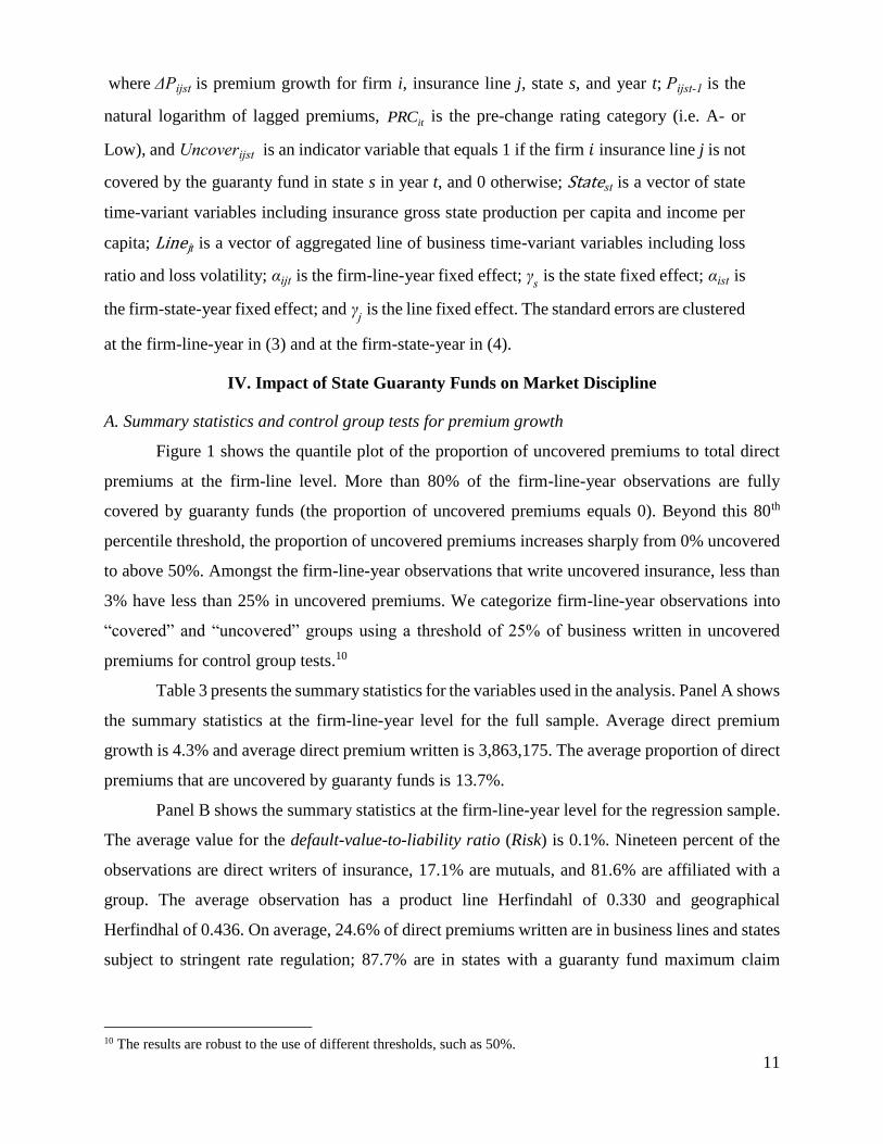
Second, guaranty funds do not pay claims beyond maximum amounts. The maximum claim

amount ranges from $100,000-$5,000,000. Table 1 shows that a majority of states have a

maximum amount in the $300,000-$500,000 range. In most states, the caps do not apply to workers

compensation insurance, and some states establish separate guaranty funds for workers

compensation. Third, some states apply policyholder net worth provisions, in which claims are not

paid for policyholders that have a net worth that exceeds specified levels. The typical net worth

provision is $25,000,000, the net worth cap ranges from $5,000,000 to $50,000,000 (see Table 1).

Fourth, the policyholders of insurers not licensed in the state (surplus lines insurers) are not

covered by guaranty funds. Surplus lines insurers underwrite risks that do not meet the

underwriting guidelines of licensed insurers or require specialized coverage, pricing or

underwriting. Surplus lines insurers have flexibility both in contract language and pricing that

2 New York uses a pre-funding model instead of an ex-post funding model. 3 Several states changed their excluded lines during our sample years. For example, NV started to exclude financial

guaranty, warranty and credit in 1993; OH started to exclude financial guaranty, fidelity and credit in 1994; and PA

started to exclude financial guaranty and warranty in 1995. 4 Accident and health insurance is excluded in all but five (5) states: MI, MT, WA, WV, WI , and WY. Credit is

excluded in all but two (2) states: MD and MI. Fidelity is excluded in all but eighteen (18) states: AL, AZ, AR, KS,

KY, ME, MD, MI, MN, MT, NM, NY, OK, OR, VT, WA WV, and WY. Financial guaranty is excluded by all but

twelve (12) states: AL, AZ, KS, MD, MI, MT, NJ, OR, VT, WA, WV, and WY. Mortgage guaranty is excluded by

all but one (1) state: MI. Ocean Marine is excluded in all but six (6) states: AK, KS, ME, MD, MI, and NY. Surety is

excluded in all but eight (8) states: AR, KS, KY, ME, MD, MI, MN, and NY. Title is excluded in all but eight (8)

states: AL, AK, CO, MD, MI, NH, NY, and ND. Warranty is excluded in all but nineteen (19) states: AL, CA, CO,

CT, KS, MD, MI, MT, NE, NH, NJ, NM, NY, OK, OR, VT, WA,WV, and WY.

6

allow them to underwrite a variety of risks---including ones that are unusual and/or substandard--

that do not conform to typical insurer appetites.

Guaranty funds can be viewed as providing a put option on the value of the insurer’s assets

with a strike price equal to the value of the insurance policies (e.g. Cummins, 1988). The flat rate

premiums in New York and the post-assessment schemes of the other states do not reflect insurer

risk. Lee, et al. (1997) and Downs and Sommer (1999) find that stock insurers increased their asset

risk with the enactment of guaranty-fund laws.

II. Data and Sample Construction

We use data from the National Association of Insurance Commissioners (NAIC) annual

statement database for the period 1989-2012. The database contains underwriting and financial

information for all U.S P/L insurers. Our analysis is based on affiliated and unaffiliated single

insurers. The Exhibit of Premiums Written (Schedule T) in the annual statement documents the

states in which the insurer is licensed and the amount of business an insurer (licensed or unlicensed)

writes in each state and line of business. We also collect other firm level information including

total assets, leverage, business diversification, and firm demographics such as organizational form,

distribution channel, and whether the insurer is affiliated with a group of insurers. The other firm

data are obtained on a calendar-year basis.

We use A.M. Best rating changes to proxy insurer financial strength changes. The

insurance market is evaluated by several credit rating agencies such as A.M. Best, Fitch, Moody’s

and Standard and Poor’s (S&P). Among them, A.M Best has, by far, the most comprehensive

coverage over the sample period. From A.M. Best’s Insurance Reports, Property-Casualty Edition

and Best’s Key Rating Guide, we obtain insurer financial strength ratings from 1989 to 2011.

Similar to Epermanis and Harrington (2006), we use rating changes to proxy for changes in insurer

default risk. The financial strength ratings are on a scale from A++ (the highest) to F (the lowest).

Bohn and Hall (1997) find that insurers approaching insolvency have unusually high premium

growth two years prior to failure. As a result, we exclude the small number of insurers with

financial strength ratings below C- (less than 0.1% of total observations).5 Firm-year observations

in which the firm was not assigned a rating by A.M. Best – for reasons such as insufficient size,

company request, or failure to submit an NAIC annual statement – are excluded from our analysis,

as are observations rated on the parallel Financial Performance Rating (FPR) scale that was used

5 All of the results are robust to the inclusion of these very low-rated firms (rated as D, E and F).

7

during the 1990’s. A.M Best updates ratings throughout the year with most changes occurring

before July. To allow comparability with other studies (e.g., Epermanis and Harrington, 2006), we

treat any rating change from August of last year through July of this year as a rating change in this

year, and any rating change after August of this year as a rating change in the next year. Table 2

shows A.M. Best ratings and how we categorize the ratings into high (above A-), A-, and low

(below A-) ratings.

We match the insurer data with guaranty fund data in the P/L insurance industry. The

guaranty fund data has been hand collected from the following sources: the National Conference

of Insurance Guaranty Funds, state insurance divisions, and the session laws and compiled statutes

of the various states.

To be included in the sample, firms must have positive direct and net premiums written

and write business in a certain line in the three years around a rating change (i.e. year t-1, t, t+1).7

Insurers that specialize in reinsurance or international business are excluded. The original sample

has 4,615,898 firm-line-year-state level observations and is aggregated to 245,934 firm-line-year

level observations with many observations being zero in premiums written. The sample screens

described above reduce the sample to 147,999 firm-line-year level observations. The inclusion of

lagged rating variables in our regressions further reduces the sample to 142,250 firm-line-year

level observations. In our analysis of the impact of market discipline on prices, we exclude all

observations with negative prices. This step reduces the price sample to 120,533 observations at

the firm-line-year level. All variables are winsorized at the 1% and 99% levels to mitigate the

effect of outliers.

III. Identification strategy

A. Firm-line level specification

Our identification strategy is to exploit the features of guaranty funds that vary across the

states and time. The variations in guaranty fund coverage are quasi-natural experiments—they

directly protect insureds but are exogenous to the insurers’ financial strength. We first examine

how government guarantees and rating changes affect premium growth at the firm-line level, with

controls for firm observed and unobserved (invariant) heterogeneity, line of business unobserved

(invariant) heterogeneity and unobserved time heterogeneity. Insurance lines with a higher

proportion of premiums not covered by guaranty funds are hypothesized to be more risk sensitive

6 Since our unit of analysis is at firm-line-year level, as long as a firm writes the same line of business in any of the

50 states in the three years surrounding rating change, it is included in our sample.

8

and, thereby, more affected by rating changes. To measure this effect, we aggregate direct written

premiums to the firm-line-year level to obtain total direct premiums, direct premiums not covered

by guaranty funds (called uncovered premiums) and direct premiums covered by guaranty funds

(called covered premiums).6 Specifically, we calculate 𝑃𝑟𝑜𝑝𝑖𝑗𝑡 as the proportion of direct

premiums written not covered by guaranty funds to total direct premiums written at the firm-line-

year.

A potential concern with the research design is that premium changes may happen before

changes in firm financial strength ratings. First, unfavorable changes in the insurance market (e.g.

large catastrophes) could deplete insurer capital and lead to changes in premium growth and

financial strength ratings. Second, insurers could begin to cut unprofitable business or expand

profitable business before the rating agency discloses new information. For example, an insurer

that anticipates a weak operating environment in the future may respond by reducing the amount

of business they write, while firms that anticipate a strong operating environment may expand.

Third, unobservable firm and line of business heterogeneity could be correlated with both premium

growth and rating changes. Fourth, premium growth could result from private information and an

anticipated change in an insurer’s rating.

To address these concerns, we use three strategies. First, to address unfavorable changes

in the environment for writing insurance we include indicator variables for one-year leaded,

contemporaneous, and one-year lagged rating changes (i.e. rating change indicators in t-1, t, and

t+1). We interact these indicators with guaranty fund coverage in the previous year to identify

evidence on market discipline across different levels of protected financing. The strategy of using

leading and lagged indicators is also employed by Epermanis and Harrington (2006). The one year

lagged rating change is used to account for the ex post effects of the rating change. The coefficients

of leaded variables provide insight into whether market discipline occurs in the year prior to a

rating change. The differences among the coefficients of the leaded, contemporaneous, and lagged

rating change variables provide information on whether market discipline occurs before, during,

or after the year of the rating change. Second, to address the concern that the proportion of

uncovered premiums may vary through time and correlated with error, we use the lagged value of

the proportion of uncovered premiums. We also include the interaction of a linear time trend with

7 For example, suppose Insurer ABC writes direct business in Other Liability insurance in three states in 2009:

$1,000,000 in Michigan, $1,500,000 in Wisconsin, and $200,000 in Illinois. Insurer ABC, however, is not licensed in

Illinois, so it writes business as a surplus lines insurer. The total direct premiums are $1,000,000 + $1,500,000 +

$200,000 = $2,700,000. The uncovered premiums are $200,000 and the covered premiums are $2,500,000.

9

the proportion of uncovered premiums in the regressions. Third, to further control for the

possibility that the insurers and markets anticipate rating changes we include a non-ratings based

measure of firm risk. In particular, we include the variable, Anticipation, which is the average

value of default-value-to-liability ratio (Risk) for the year’s t-1 and t-2.8

The main estimating equation is:

ijttijpostit-1ijtpostcurrentit-1ijtcurrent

preit-1ijtpreitd-1ijtpijtijt

Prop'Prop'

Prop'I'+Prop+change) rating no|PE(P

,,

,

11

1 (1)

where ijtP is premium growth for firm i, line j and year t; Propijt

is the proportion of direct

premiums written not covered by guaranty funds to total premiums. Specifically, we measure

premium growth using direct premiums written since net premiums written (premium net of

reinsurance) is not available at the state level. Growth in direct premiums written (∆Log Premium)

is measured as the first difference of the log of direct premium written by insurer 𝑖 at time 𝑡 and

the log of direct premium written by insurer i at time t-1. The premium growth measures are

censored at -1 and 1. 1it, pre , 1it,current, and 1it,post are vectors of binary variables equal to 1 for lead

rating changes, contemporaneous changes, and lagged changes (upgrade or downgrade) for firm 𝑖

in year t. Iit is the stack vector of these binary variables. The γij represents a firm-line fixed effect,

which absorbs unobservable differences at the firm and line of business level; δt is a year fixed

effect, and εijt is an error term.

The expected premium growth conditional on no rating change is:

ijtit-1ijt10ijt XPchange) rating no|PE( 2' (2)

where Pijt-1 is lagged log premiums; Xit is a vector of covariates that includes controls for firm time

variant characteristics such as asset, leverage, reinsurance, geographical diversification, line of

business diversification, organizational form, direct writer, premiums subjected to prior approval

rate regulation and rating categories (A- or LOW) in the previous year (see extended models in

Table 8 for more details), and also guaranty fund related controls such as claim caps and net worth

provisions.9 This research design allows us to account for both the time-invariant characteristics

of firm and lines of business and the time-varying characteristics of firms.

β'current

and β'post

in equation (1) capture the current and post yearly premium growth

percentage response to a change in the proportion of uncovered premiums for a firm-line-year

8 The precise definition of the variable Anticipation is in Appendix A. 9 The hypotheses and precise definitions of the control variables can be found in Appendix A.

10

experiencing a rating change, relative to the current and post premium growth of the control group

(those with Propijt-1=0 ), respectively. β'

pre measures the difference in the premium growth

between the firm-line with positive Propijt

and the control group one year before the firm-line

experiences a rating change. Evidence that government guarantees dull market discipline requires

that the difference between β'pre

and β'current

(or β'post

) to be statistically and economically

distinguishable from zero. We also extend equation (1) to incorporate the effects of the A.M. Best

rating category (High, A-, Low).

B. Firm-line-state level specification

Many insurers operate the same line of business in multiple states and/or operate multiple

lines in one state, providing insurance to both protected and unprotected customers. Thus, we can

use data on the firm-line-state-year level to further control for potentially confounding effects and

to detect the source of variation, by using business that is protected by a guarantee fund as a control

group. To be included in these regressions, a firm-line-state-year observation is required to be

downgraded in that year. We run the regressions two ways. The first regression includes a firm-

line-year fixed effect and a state fixed effect. The firm-line-year fixed effect sweeps out the

variation between firm-lines, making the estimates based on only the variation within each firm-

line and across states. Within firm-line variation occurs when a given firm-line has premiums in

two or more states whose guaranty fund protection differs at least once during the sample period.

The primary source of identification is driven by surplus lines insurers, i.e., insurance firms that

are not licensed in some states and therefore not covered by guaranty funds. A secondary source

of identification is the lines of insurance that receive guaranty fund coverage in some states but

not others (see footnote 4). The second regression includes a firm-state-year fixed effect and a line

fixed effect. The firm-state-year fixed effect sweeps out the between firm-state variation, and the

effect of guaranty funds is identified on the basis of protection differences within a firm operating

multiple lines of business in a state. In other word, the regression tests for variation across line of

business within each firm and state. Specifically, we estimate the following models:

State variations:

ijststsitijstuijstsijtijst StatePRCerUnPP

''

11 cov (3)

Insurance line of business variations:

ijstjtjitijstuijstjistijst LinePRCerUnPP

''

11 cov (4)

11

where ΔPijst is premium growth for firm i, insurance line j, state s, and year t; Pijst-1 is the

natural logarithm of lagged premiums, itPRC is the pre-change rating category (i.e. A- or

Low), and Uncoverijst is an indicator variable that equals 1 if the firm 𝑖 insurance line j is not

covered by the guaranty fund in state s in year t, and 0 otherwise; Statest is a vector of state

time-variant variables including insurance gross state production per capita and income per

capita; Linejt is a vector of aggregated line of business time-variant variables including loss

ratio and loss volatility; αijt is the firm-line-year fixed effect; γs is the state fixed effect; αist is

the firm-state-year fixed effect; and γj is the line fixed effect. The standard errors are clustered

at the firm-line-year in (3) and at the firm-state-year in (4).

IV. Impact of State Guaranty Funds on Market Discipline

A. Summary statistics and control group tests for premium growth

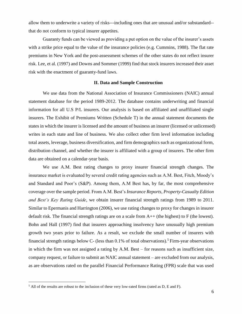
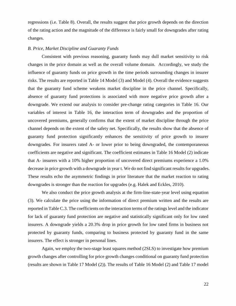
Figure 1 shows the quantile plot of the proportion of uncovered premiums to total direct

premiums at the firm-line level. More than 80% of the firm-line-year observations are fully

covered by guaranty funds (the proportion of uncovered premiums equals 0). Beyond this 80th

percentile threshold, the proportion of uncovered premiums increases sharply from 0% uncovered

to above 50%. Amongst the firm-line-year observations that write uncovered insurance, less than

3% have less than 25% in uncovered premiums. We categorize firm-line-year observations into

“covered” and “uncovered” groups using a threshold of 25% of business written in uncovered

premiums for control group tests.10

Table 3 presents the summary statistics for the variables used in the analysis. Panel A shows

the summary statistics at the firm-line-year level for the full sample. Average direct premium

growth is 4.3% and average direct premium written is 3,863,175. The average proportion of direct

premiums that are uncovered by guaranty funds is 13.7%.

Panel B shows the summary statistics at the firm-line-year level for the regression sample.

The average value for the default-value-to-liability ratio (Risk) is 0.1%. Nineteen percent of the

observations are direct writers of insurance, 17.1% are mutuals, and 81.6% are affiliated with a

group. The average observation has a product line Herfindahl of 0.330 and geographical

Herfindhal of 0.436. On average, 24.6% of direct premiums written are in business lines and states

subject to stringent rate regulation; 87.7% are in states with a guaranty fund maximum claim

10 The results are robust to the use of different thresholds, such as 50%.

12

amount of $300,000 or more; and 41.1% are in states with net worth provisions beyond

$25,000,000.

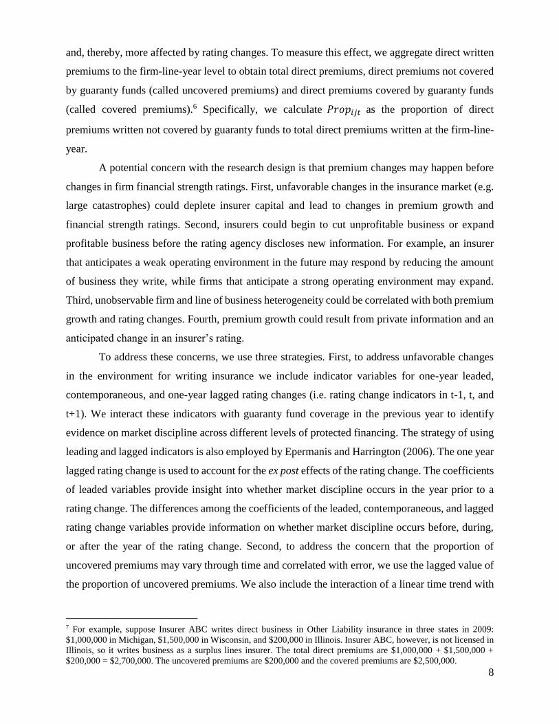
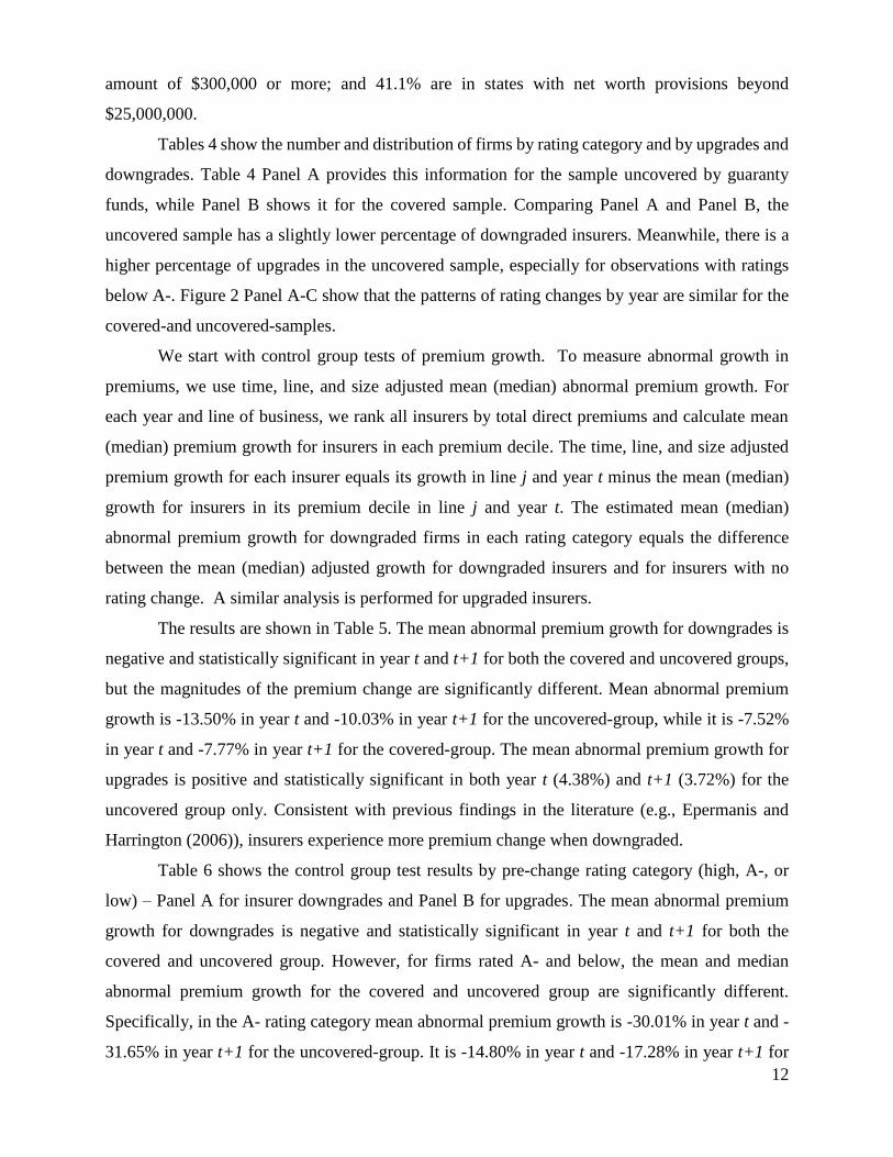
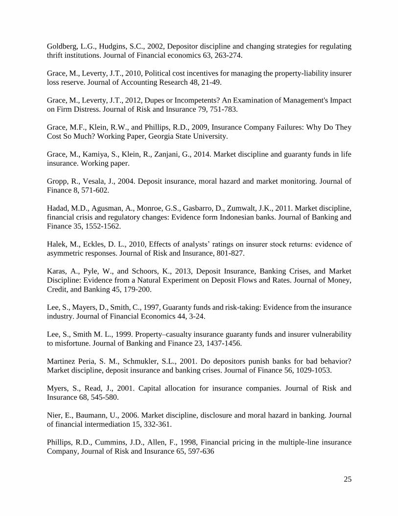
Tables 4 show the number and distribution of firms by rating category and by upgrades and

downgrades. Table 4 Panel A provides this information for the sample uncovered by guaranty

funds, while Panel B shows it for the covered sample. Comparing Panel A and Panel B, the

uncovered sample has a slightly lower percentage of downgraded insurers. Meanwhile, there is a

higher percentage of upgrades in the uncovered sample, especially for observations with ratings

below A-. Figure 2 Panel A-C show that the patterns of rating changes by year are similar for the

covered-and uncovered-samples.

We start with control group tests of premium growth. To measure abnormal growth in

premiums, we use time, line, and size adjusted mean (median) abnormal premium growth. For

each year and line of business, we rank all insurers by total direct premiums and calculate mean

(median) premium growth for insurers in each premium decile. The time, line, and size adjusted

premium growth for each insurer equals its growth in line j and year t minus the mean (median)

growth for insurers in its premium decile in line j and year t. The estimated mean (median)

abnormal premium growth for downgraded firms in each rating category equals the difference

between the mean (median) adjusted growth for downgraded insurers and for insurers with no

rating change. A similar analysis is performed for upgraded insurers.

The results are shown in Table 5. The mean abnormal premium growth for downgrades is

negative and statistically significant in year t and t+1 for both the covered and uncovered groups,

but the magnitudes of the premium change are significantly different. Mean abnormal premium

growth is -13.50% in year t and -10.03% in year t+1 for the uncovered-group, while it is -7.52%

in year t and -7.77% in year t+1 for the covered-group. The mean abnormal premium growth for

upgrades is positive and statistically significant in both year t (4.38%) and t+1 (3.72%) for the

uncovered group only. Consistent with previous findings in the literature (e.g., Epermanis and

Harrington (2006)), insurers experience more premium change when downgraded.

Table 6 shows the control group test results by pre-change rating category (high, A-, or

low) – Panel A for insurer downgrades and Panel B for upgrades. The mean abnormal premium

growth for downgrades is negative and statistically significant in year t and t+1 for both the

covered and uncovered group. However, for firms rated A- and below, the mean and median

abnormal premium growth for the covered and uncovered group are significantly different.

Specifically, in the A- rating category mean abnormal premium growth is -30.01% in year t and -

31.65% in year t+1 for the uncovered-group. It is -14.80% in year t and -17.28% in year t+1 for

13

the covered-group. The difference between the uncovered and covered-groups is -14.22% and -

14.37% in year t and t+1, respectively. For low rated firms, mean abnormal premium growth is -

26.01% in year t and -17.01% in year t+1 for the uncovered-group and -13.04% and -11.61% for

the covered-group. The difference is -12.96% in year t and -5.40% in year t+1. The difference in

mean and median abnormal premium growth between the two groups in year t-1 is not statistically

significant for downgrades, suggesting that there is no pattern change in premiums prior to the

downgrade. The results indicate that the uncovered-group experiences more negative mean

abnormal premium growth with a rating downgrade compared to the covered-group.

The results in Panel B show that with a rating upgrade low rated firms in the uncovered-

group experience significantly greater mean abnormal premium growth than the covered-group.

In particular, mean abnormal premium growth is 18.52% in year t and 13.52% in year t+1 for the

uncovered group, while it is 2.75% and 7.44% for the covered group. The difference is 15.76% in

year t and 6.07% in year t+1. Overall, the results are consistent with the hypothesis that the

presence of guaranty fund protection reduces the sensitivity of premium growth to changes in

insurer’s financial strength ratings.

B. Regression results at the firm-line-year level

Negative signs on the A- and LOW rating dummies are consistent with market discipline.

A negative (positive) estimate of βd

' for the lagged or contemporaneous downgrade (upgrade)

indicators is also interpreted as evidence of market discipline. A significant positive (negative)

estimate of βp would indicate that the higher the proportion of uncovered premiums the higher

(lower) the premium growth. The interaction of the proportion of uncovered premiums variable

with the vector of rating changes estimates whether guaranty funds reduce market discipline.

Specifically, a negative and significant βcurrent

and βpost

would suggest that the presence of

guaranty fund protection reduces market discipline, i.e., guaranty funds dull the risk sensitivity of

demand.

Table 7 reports the least squares and fixed effects estimates of the model described by

equations (1) and (2) for direct premium growth. Model (1) reports the OLS results, Model (2)

shows the results with firm-line, and year fixed effects, Model (3) adds “Anticipation” and firm

and guaranty fund controls. In order to account for the possibility that the size of the insurer

influences the effect of market discipline, we use weighted fixed effects in Model (4).11 Model (5),

11 We divide the insurers into ten ranked groups based on their average premium written across years. We assign the

number 1-10 to each group and use them as weights.

14

which we discuss in detail below, is a 2SLS regression, which is designed to address the concern

that changes in the proportion of uncovered premiums may arise endogenously with rating changes.

The implications of the regressions are broadly consistent with those of the control group

tests, but the magnitudes of the estimated coefficients on the rating change variables are smaller

in the fixed effects regressions. A Hausman test rejects the null hypothesis that differences in the

coefficients of OLS and fixed effects are not systematic, suggesting the fixed effects approach is

appropriate. The results are robust to the inclusion of the firm and guaranty fund controls and to

the interaction of the linear year trend with the proportion of uncovered premiums. The results

support the hypothesis that guaranty fund protection reduces policyholder sensitivity to risk---the

coefficients for βcurrent

are about -0.047 for downgraded insurers and 0.034 for upgraded insurers

in Model (2). The coefficient on Anticipation is not significant in all Models, indicating that market

anticipation of the insurer risk change is weak. We get similar results using weighted fixed effects

(Model (4)). The magnitudes which guaranty funds dull risk sensitivity are marginally higher in

the weighted fixed effects model.

Table 8 extends equations (1) and (2) by incorporating pre-change rating categories. The

coefficients in fixed effects model for βpre

provide little evidence that premium growth the year

prior to a rating change varies with the proportion of uncovered premiums. The coefficients for

βcurrent

for A- insurer downgrades (-0.200) and βcurrent

for Low insurer downgrades (-0.143) are

significantly negative, indicating that firm-lines with relatively higher proportion of uncovered

premiums experience more negative premium reactions to downgrades, ceteris paribus.

Economically, the coefficient in year t for the downgrade of an A- rated insurer implies

that a 10% increase in the proportion of uncovered premiums is associated with 2.0% decrease in

premium growth to a downgrade action. Given that the difference between the average proportion

of uncovered premiums for the covered- and uncovered-group is approximately 86% (see the table

attached to Figure 1) and statistically significant, the A- rated uncovered-group would, on average,

be associated with -17.2% premium growth with a downgrade in year t. The low rated uncovered-

group would, on average, experience -12.3% premium growth with a downgrade in year t. These

results suggest that guaranty funds dull the risk sensitivity of financing costs when insurers are

downgraded. Similarly, the coefficient on the interaction variable for low rated insurer upgrades

is 0.070, suggesting that, on average, the low rated uncovered-group realizes 6.0% additional

premium growth with upgrades in year t.

15

While the features of guaranty funds in each state (i.e. which lines are covered, the

maximum claim amount, and the net worth provisions) are exogenous for individual insurers, it is

possible that the proportion of uncovered premiums is endogenous, as insurers that experience

downgrades may rely more on covered business, and vice versa.12 To deal with this potential

problem, we use an instrumental variables (2SLS) procedure based on the weighted fixed effects

model. The first stage regression instruments the proportion of uncovered premiums with its value

lagged by three years, Mutual, Group, Busherf, and Geoherf. The R2 of the first regression (not

reported here) is around 0.89. The predicted value of the first-stage regression is then used in the

second stage regression instead of the actual value. The results, shown in Table 8 Model (5),

indicate that the magnitude by which guaranty funds dull risk sensitivity is marginally higher than

the original weighted fixed effects model.

We run Table 7 model (3) by line of business, and the results are shown in Table 9. We

find directionally consistent and statistically significant guaranty fund effects on market discipline

in Commercial Multiple Peril and Other Liability. Other lines also exhibit directionally consistent

effects, although they are not statistically significant.

C. Regression results at the firm-line-state-year level

Table 10 Column 1 shows the regression results for equation (3) for all lines. The

coefficients on the interaction terms of the ratings level and the indicator for lack of guaranty fund

protection are negative and statistically significant for A- and low rated insurers. A downgrade

yields a 15.2% drop in premium growth for A- rated firms and a 9.7% drop for low rated firms in

lines of insurance not protected by guaranty funds.

To see whether this state-variation effect is driven by non-traditional lines of insurance, we

re-do the analysis using only traditional lines of insurance or only non-traditional lines. We classify

non-traditional lines of insurance as credit, surety, fidelity, financial guaranty, mortgage guaranty,

ocean marine, warranty, and title insurance. These are the lines of insurance that are most

commonly not covered by guaranty funds. Column 2 shows the results using the traditional lines

of insurance. Column 3 shows the results for non-traditional lines. For traditional lines, the

coefficients on the interaction terms of ratings level and the indicator for lack of guaranty fund

protection are negative and statistically significant for downgrades of A- and low rated firms. A

12 A significant proportion of insurance that is not covered by guaranty funds belongs to insurers with stable business

or to insurers with a particular organizational structure, e.g. risk retention groups. It is important to note that a number

of insurance entities that do not receive guarantee fund coverage (e.g., risk retention groups) are establsihed to provide

stable and dependable coverage to their policyholders.

16

downgrade yields a 21.2% drop in premium growth for A- rated firms. The drop is 11.9% for low

rated firms. For non-traditional lines, the coefficients on the interaction terms of ratings level and

the indicator for lack of guaranty fund protection are negative and statistically significant for

downgrades. A downgrade yields a 3.0% drop in premium growth for high rated firms, a 7.9%

drop for A- rated firms and an 8.4% drop for low rated firms. The results indicate that the effect

of guaranty funds is not being driven by non-traditional lines of insurance. In fact, the magnitudes

of the declines are greater for traditional lines than non-traditional lines. The results also indicate

that customer sensitivity to risk is greater for lower rated insurers in traditional lines, but higher

for higher rated insurers in non-traditional lines, suggesting that financial quality is perhaps more

important in non-traditional lines.

Columns 4 and 5 test state variation for personal lines and commercial lines.13 The results

imply that guaranty funds mainly influence downgrades in commercial lines. The results are in

line with the findings in Epermanis and Harrington (2006) that market discipline works more in

commercial lines than personal lines.

As shown in Table 11 (line of business variation model described in equation (4)), a

downgrade yields a 5.8% drop in premium growth for high rated firms and 5.3% for A- rated firms

in lines of insurance not protected by guaranty funds. A downgrade also yields a 5.5% drop in

premium growth for low rated firms. The effect is also manifest in nontraditional and commercial

lines.

In Table 10 and Table 11, the effects are from insurers writing both covered and uncovered

business at the same time, i.e. insurers in the same firm and line of business but writing business

in different states, or insurers in the same firm and state but writing business in different lines. We

find premium declines greater in the uncovered business following downgrades. Thus we find that

guaranty funds shield insurers from the full costs of market discipline.

D. Robustness checks

D.1 The internal valid check and dynamic impact of rating changes

The main concerns to our first research design are (1) the correlation between the timing

of rating changes and the time-path of premium growth, (2) rating changes being anticipated by

the insurance market, and (3) the different patterns of premium growth before rating changes

across the different levels of guaranty fund protection. To further provide supporting evidence that

13 Personal lines include farm owners multiple peril, homeowners multiple peril, private passenger auto liability, and

private auto physical damage; commercial lines include everything else.

17

our results are valid, we perform internal validity checks. To formally test whether (1)-(3) are

impacting our results we introduce pre-rating change leads. Moreover, to study the effect of rating

changes over time, we add post-rating change lags. The effect of risk changes is likely to diminish

over time as the insurer and policyholders adjust to a new reality.

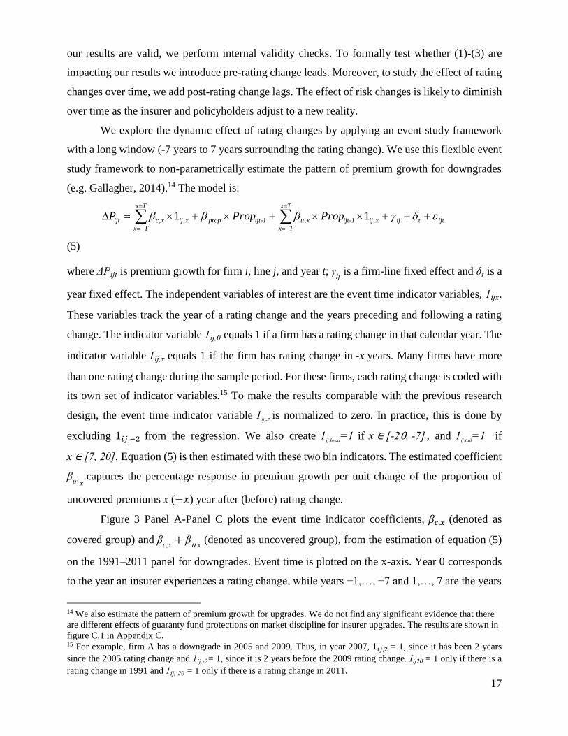
We explore the dynamic effect of rating changes by applying an event study framework

with a long window (-7 years to 7 years surrounding the rating change). We use this flexible event

study framework to non-parametrically estimate the pattern of premium growth for downgrades

(e.g. Gallagher, 2014).14 The model is:

ijt

Tx

Tx

tijxij1-ijtxu1-ijt

Tx

Tx

propxijxcijt PropPropP

,,,, 11

(5)

where ΔPijt is premium growth for firm i, line j, and year t; γij is a firm-line fixed effect and δt is a

year fixed effect. The independent variables of interest are the event time indicator variables, 1ijx.

These variables track the year of a rating change and the years preceding and following a rating

change. The indicator variable 1ij,0 equals 1 if a firm has a rating change in that calendar year. The

indicator variable 1ij,x equals 1 if the firm has rating change in -x years. Many firms have more

than one rating change during the sample period. For these firms, each rating change is coded with

its own set of indicator variables.15 To make the results comparable with the previous research

design, the event time indicator variable 1ij,-2 is normalized to zero. In practice, this is done by

excluding 1𝑖𝑗,−2 from the regression. We also create 1ij,head

=1 if x ∈ [-20, -7] , and 1ij,tail

=1 if

x ∈ [7, 20]. Equation (5) is then estimated with these two bin indicators. The estimated coefficient

βu,x captures the percentage response in premium growth per unit change of the proportion of

uncovered premiums x (−𝑥) year after (before) rating change.

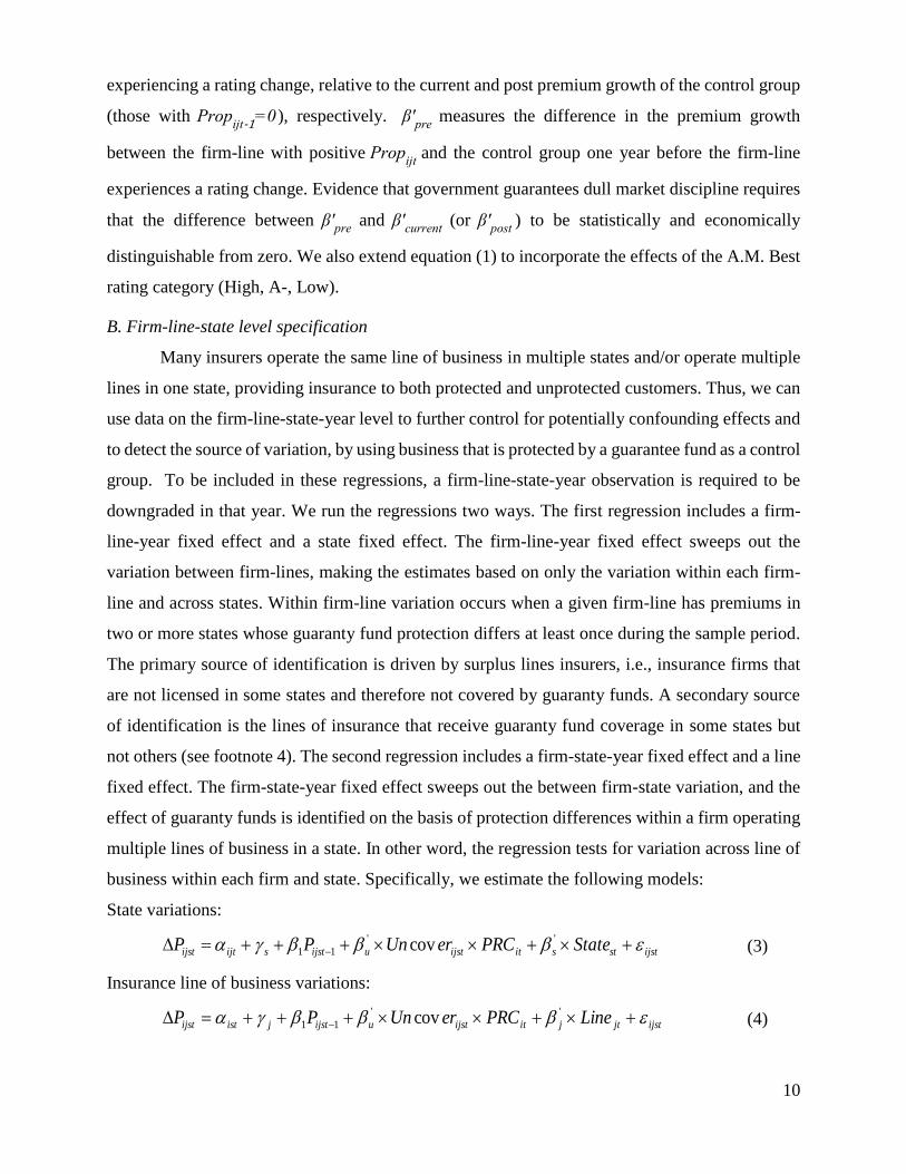
Figure 3 Panel A-Panel C plots the event time indicator coefficients, 𝛽𝑐,𝑥 (denoted as

covered group) and βc,x

+ βu,x (denoted as uncovered group), from the estimation of equation (5)

on the 1991–2011 panel for downgrades. Event time is plotted on the x-axis. Year 0 corresponds

to the year an insurer experiences a rating change, while years −1,…, −7 and 1,…, 7 are the years

14 We also estimate the pattern of premium growth for upgrades. We do not find any significant evidence that there

are different effects of guaranty fund protections on market discipline for insurer upgrades. The results are shown in

figure C.1 in Appendix C. 15 For example, firm A has a downgrade in 2005 and 2009. Thus, in year 2007, 1𝑖𝑗,2 = 1, since it has been 2 years

since the 2005 rating change and 1ij,-2= 1, since it is 2 years before the 2009 rating change. Iij20 = 1 only if there is a

rating change in 1991 and 1ij,-20 = 1 only if there is a rating change in 2011.

18

before and after the rating change, respectively. The plotted event time coefficients can be

interpreted as the percent change in premium growth relative to two years prior to the rating change.

The bands represent the 95 percent confidence interval and show whether each point estimate is

statistically different from 0.

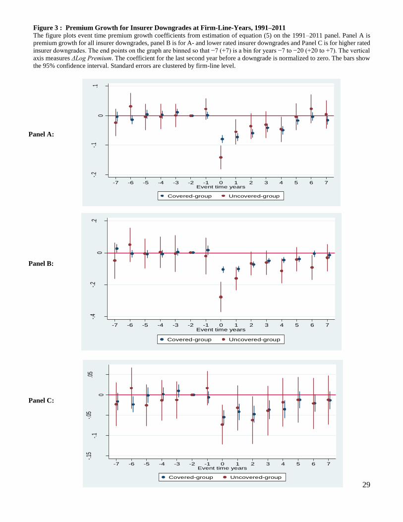
There is no discernable trend in premium growth in the years before a rating change.

Premium growth is lowest in the year of a downgrade—a 12 percent decrease for the uncovered

group and a 7 percent decrease for the covered group. After a downgrade premium growth remains

negative and statistically significant for four years. After four years, premium growth is not

statistically different from zero. The difference in the impulse responses between the uncovered

and covered groups, however, disappears after one year. The same pattern of decline in insurance

premium growth repeats if an insurer has multiple downgrades during the period. The effect of

downgrades on premium growth is transitory; however, the shock to total premium, is “permanent”:

on average, total premium is decreased by 0.5 million for uncovered business the year at a

downgrade. Overall, the patterns shown in Figure 3 are in line with the results in Table 8--- the

premium decline for A- and low-rated insurers is significantly greater for the uncovered group

than the covered group in the year of a downgrade. We also estimate the pattern of premium growth

for upgrades. We do not find any significant evidence that there are different effects of guaranty

fund protections on market discipline for insurer upgrades (shown in Appendix Figure C.1).

D.2 Test for an alternative explanation

Another potential concern is that covered business and uncovered business may differ in

their business characteristics and in particular their profitability and riskiness. Firms may reduce

their exposure to less profitable or higher risk business after a downgrade. Thus, the observed drop

in uncovered business may be due to changes in the composition of the insurer’s underwriting

portfolio and not because of guaranty fund protection. We investigate the alternative explanation

in two ways. First, we examine whether uncovered business is more or less profitable than covered

business. We test whether the mean value of the ratio of losses to premiums (the loss ratio) differs

by guaranty fund status. A higher loss ratio implies less profitable business. We first divide all

insurers’ business into covered business and uncovered business at the firm-line-state-year level.

We then aggregate direct losses incurred and direct premium earned for covered and uncovered

business, at the line and year level. We then divide aggregate losses by aggregate premiums. Table

12 reports differences in the means by guaranty fund covered status. In general, the results show

that the loss ratio of uncovered business is largely the same as the loss ratio of covered business.

19

We do not find significant differences in the mean values of the loss ratio between covered business

and uncovered business, except for workers compensation, special liability and warranty. We find

the mean value of the loss ratio is higher for uncovered business in workers compensation, 16 but

the measure is lower for uncovered business in special liability and warranty. Based on these

results, we cannot conclude that uncovered business is more or less profitable than covered

business.

Second, we examine whether premium growth differs by the risk characteristics of business

surrounding rating changes. If our results are driven by downgraded insurers’ trimming risky

business, then we should observe that behavior across all lines of business (i.e., firms would also

cut back on riskier covered business). To examine riskiness, we calculate the variance of the loss

ratio by line of business (shown in Table 12). A more volatile loss ratio suggests a higher risk line

of business (Lamm-Tennant and Starks, 1993). We sort the lines of business into high and low risk

groups – if the variance of the loss ratio is in the top seven lines among the 14 lines it is classified

as high risk and it is in the bottom then it is classified as low risk.17 The seven high risk lines are

homeowners/farmowners, medical malpractice, special liability, special property, fidelity/surety,

product liability and financial guaranty/mortgage guaranty. We run two models using our previous

identification strategies. First, we calculate the proportion of high risk business as the fraction of

direct premiums written of high risk business to total direct premiums written and repeat our first

identification strategy in equation (1) and (2). As shown in the Table 13 Panel A, we do not identify

any negative coefficients on interactions of downgrades and the proportion of high risk business.

Second, we use data on the firm-line-state-year level. To be included in these regressions, a firm-

line-state-year observation is required to be downgraded in that year. We run the regressions

similar to equation (4) but we include a firm-year fixed effect, a state fixed effect and a line of

business fixed effect. The firm-year fixed effect sweeps out the variation between firms, making

the estimates based on only the variation within each firm across line of business and states. We

use a dummy variable High Risk Business, which equals one to indicate if the business is high risk,

16 We exclude workers compensation and repeat our previous analyses. All of our results are robust. 17 We also examine whether the variances of the loss ratio differ significantly by guaranty fund status. To avoid the

issue that the volatility of the loss ratio is caused primarily by significantly less premium volume in uncovered lines

than their covered counterparts, we conduct the analysis for insurers having both uncovered business and covered

business. Table C.2 reports the means and variances of the loss ratio by guaranty fund covered status across lines over

the sample period. In general, the results show that the business characteristics of uncovered business and covered

business are largely the same. We do not find significant differences in the variances of the loss ratio between covered

business and uncovered business, except for homeowners/farmowners, product liability and special liability. We find

the variances of the loss ratio are higher for the uncovered business in homeonwers/farmowners, but the measure is

lower for uncovered business in special liability and product liability.

20

and 0 otherwise. The results are shown in Table 13 Panel B. We again do not find any negative

coefficients on the interactions of the pre-change rating categories and High Risk Business. These

results suggest that the greater premium declines in uncovered business relative to covered lines

are not driven by insurers changing the risk composition of their underwriting portfolios.

V. Prices, Market Discipline, and Government Guarantees

A. Prices and Market Discipline

In this section we explore evidence on the nexus between prices and market discipline.

Evidence in this paper has shown that increases in insurer risk are accompanied by reductions in

premium growth. This could be because firms are forced to lower prices, or their business volume

drops, or both. Accordingly, policyholders can exert market discipline by buying less coverage,

not buying insurance, or demanding a lower price from a downgraded insurer. Insurers may

respond to market discipline as well, but not all insurers have the same flexibility. Insurers subject

to stringent rate regulation may not be able to adjust prices (Grace and Leverty, 2010).

We study the relationship between insurance prices and changes in financial strength

ratings. In particular, we use equation (1) and equation (2), but replace the dependent variable,

premium growth, with price growth. We calculate insurance price growth (∆Log Price). Since

explicit contract prices are not available, we follow the literature and use an implicit measure of

price (e.g. Cummins and Danzon, 1997; Cummins et al., 2005).18 We measure price at the firm-

line level as information on business net of reinsurance is not available at firm-line-state level.19

Since premiums are revenues (price times quantity), the impact of downgrades on prices will yield

insight on the price mechanism and because we have already studied the impact on premiums, we

can impute the impact on quantity.

The results of fixed effects estimates of price growth using net business are reported in

Table 14. The regressions in Models (1) and (2) do not consider guaranty fund characteristics,

while Models (3) and (4) do. The regressions reported in Table 15 incorporate the pre-change

rating categories. We document several noteworthy price effects. First, the coefficients on all

current and leading variables in rating change indicators for downgrades are negative and

significant, providing clear evidence that insurers have slower price growth the year before and

the year of a downgrade. The coefficients on Anticipation are negative and statistically significant,

18 The precise definition and calculation of insurance price are described in Appendix B. 19 We also calculate price using direct business (premium written and direct loss incurred) instead of net business and

our results are robust.

21

possibly indicating that insurers anticipate downgrades and adjusts prices accordingly. In Table

14, current and lagging coefficients on upgrades are positive and significant but leading variables

are not significant, indicating that price growth increases after upgrades. In Table 15, all the current

and leading coefficients on rating change indicators for downgrades are significant, suggesting

that price deterioration may precede downgrades in the market. This phenomenon can be explained

in several ways. It could be that insurers have poor underwriting results in the year before a

downgrade, which explains a drop in measured price as well as the subsequent downgrade.

Another explanation could be that the market anticipates rating deterioration, and prices adjust

accordingly. The effect of upgrades on price growth is statistically significant---upgrades are

associated with price increases for A- and low-rated insurers, with pre-rating change increases also

evident for low-rated insurers.

Second, we compare coefficients across regressions of premium growth and price growth

(results shown in Appendix Table C.1). The magnitudes of the coefficients on downgrades in the

current price growth regression are smaller than those for premium growth change for A- and

lower rated insurers.20 We find that price growth decreases significantly in the year of a downgrade,

but that the magnitude of the decrease is much smaller for price growth than it is for premium

growth in the year of insurer downgrades. The results suggest that policyholders respond to

increases in insurer risk both by demanding lower prices and by shifting their contracts. Insurance

prices, however, are only slightly affected the year after insurer downgrades, suggesting

policyholders continuously react to downgrades by switching to safe insurers.

In addition, we control for price growth in the premium growth regression, since premium

growth endogenously depends on price growth. We employ the two-stage least squares method

(2SLS) to investigate how premium growth changes after controlling price growth change (Results

are shown in Table 17, Model (1)). Predicted price growth is included in the premium growth

regression in the second step. Although the regression sample size is reduced by fifteen percent

because negative prices are excluded in our analysis, we can still identify market discipline in the

form of premium growth. The magnitudes of the coefficients on the rating change variables

estimated for premium growth rates are smaller than the previous fixed effects regressions (Table

8, Model 2). The signs of these estimated variables in 2SLS are consistent with the previous

20 We run the seemingly unrelated regression to test whether coefficients of premium growth and price growth are

significantly different. We use the sample with positive calculated insurance price, which includes 120,533

observations. The results shows the coefficients on current variables of price growth are significantly smaller than

those for premium growth model for A- and lower insurers (see Appendix C Table C.1 for details).

22

regressions (i.e. Table 8). Overall, the results suggest that price growth depends on the direction

of the rating action and the magnitude of the difference is fairly small for downgrades after rating

changes.

B. Price, Market Discipline and Guaranty Funds

Consistent with previous reasoning, guaranty funds may dull market sensitivity to risk

changes in the price domain as well as the overall volume domain. Accordingly, we study the

influence of guaranty funds on price growth in the time periods surrounding changes in insurer

risks. The results are reported in Table 14 Model (3) and Model (4). Overall the evidence suggests

that the guaranty fund scheme weakens market discipline in the price channel. Specifically,

absence of guaranty fund protections is associated with more negative price growth after a

downgrade. We extend our analysis to consider pre-change rating categories in Table 16. Our

variables of interest in Table 16, the interaction term of downgrades and the proportion of

uncovered premiums, generally confirms that the extent of market discipline through the price

channel depends on the extent of the safety net. Specifically, the results show that the absence of

guaranty fund protection significantly enhances the sensitivity of price growth to insurer

downgrades. For insurers rated A- or lower prior to being downgraded, the contemporaneous

coefficients are negative and significant. The coefficient estimates in Table 16 Model (2) indicate

that A- insurers with a 10% higher proportion of uncovered direct premiums experience a 1.0%

decrease in price growth with a downgrade in year t. We do not find significant results for upgrades.

These results echo the asymmetric findings in prior literature that the market reaction to rating

downgrades is stronger than the reaction for upgrades (e.g. Halek and Eckles, 2010).

We also conduct the price growth analysis at the firm-line-state-year level using equation

(3). We calculate the price using the information of direct premium written and the results are

reported in Table C.3. The coefficients on the interaction terms of the ratings level and the indicator

for lack of guaranty fund protection are negative and statistically significant only for low rated

insurers. A downgrade yields a 20.3% drop in price growth for low rated firms in business not

protected by guaranty funds, comparing to business protected by guaranty fund in the same

insurers. The effect is stronger in personal lines.

Again, we employ the two-stage least squares method (2SLS) to investigate how premium

growth changes after controlling for price growth changes conditional on guaranty fund protection

(results are shown in Table 17 Model (2)). The results of Table 16 Model (2) and Table 17 model

23

(2) suggest that the effect of guaranty funds on market discipline are through both the price channel

and the quantity channel.

VI. Concluding Remarks

This paper explores how government safety-net schemes affect market discipline in the

financial sector. We study the state regulated P/L insurance industry because the diversity of

guaranty fund protection offered by the states offers a compelling environment in which to identify

the effects of public guarantees. The evidence suggests that public guarantees dull customer

sensitivity to financial institution risk, and overall effects are quite large. The effects are especially

large for A- and low-rated insurer downgrades. The pattern of decline in premium growth suggests

that the process of market discipline is most pronounced within two years of downgrades.

Moreover, effect is most pronounced within commercial insurance lines.

The study is important from a public policy perspective. Policymakers are increasingly

aware of the role of market discipline in the regulation of financial firms and modern regulatory

policy tries to encourage market discipline (e.g. Solvency Modernization Initiative, Basel II and

Solvency II). In fact, both Basel and Solvency II include market discipline as a fundamental pillar

and attempt to enhance it through public disclosure of risk-related information by banks and

insurance companies. The benefit of stronger market discipline is believed to reduce the need for

government intervention. Our study finds that consumer protection schemes, even ones that

consumers are less aware of, impair market discipline, as such regulators must take these programs

into consideration in the design of solvency regulatory policy. Combined with the evidence on the

huge cost of insurer failures (Bohn and Hall, 1997; Grace, Klein and Phillips, 2009; Leverty and

Grace, 2012), our findings suggest that policy makers should address the adverse incentives that

guaranty funds create in order to better discipline insurers and protect policyholders. Potential

changes could be the creation of a first layer of private loss of guaranty fund coverage (e.g.,

coinsurance or a high deductible) or the adoption of risk-based guaranty fund assessments. The

results for the insurance industry have interesting implications for the financial sector more broadly.

This supports the view that deposit insurance and other public guarantees in banking have

significant effects on market discipline.

24

References

Billet, M., Garfinkel, J.A. and O’Neal, E.S., 1998. The cost of market versus regulatory discipline

in banking. Journal of Financial Economics 48, 333-358.

Bohn, J. G., Hall, B. J., 1995. Property and casualty solvency funds as a tax and social insurance

system. Working Paper no. 5206. Cambridge, Mass.: National Bureau of Economic Research,

August.

Bohn, J. G., Hall B. J., 1997. The moral hazard of insuring the insurers. Working Paper no. 7955.

Cambridge, Mass.: National Bureau of Economic Research, January.

Cummins, J.D., 1988. Risk-based premiums for insurance guaranty funds. Journal of Finance 43,

823-839.

Cummins, J.D., Danzon, P.M., 1997. Price, financial quality, and capital flows in insurance

markets. Journal of Financial Intermediation 6, 3-38.

Demirguc-Kunt, A., and Huizinga, H., 2004. Market discipline and deposit Insurance. Journal of

Monetary Economics 51, 375-399.

Demirguc-Kunt, A., Detragiache, E., 2002. Does deposit insurance increase banking system

stability? An empirical investigation. Journal of Monetary Economics 49, 1337–1371.

Downs, D., Sommer, D., 1999. Monitoring, ownership and risk-taking: the impact of guaranty.

Journal of Risk and Insurance 66: 477-497.

Eling, M., Schmit, J.T., 2012. Is there market discipline in the European insurance industry? An

analysis of German insurance market. Geneva Risk and Insurance Review 37,180-207.

Eling, M, 2012. What do you know about market discipline in insurance? Risk Management and

Insurance Review 15, 185-223.

Eling, M., Kiesenbauer, D., 2012, Does surplus participation reflect market discipline? An analysis

of the German life insurance market. Journal of Financial Services Research 42, 159-185.

Epermanis, K., Harrington., S, 2006. Market discipline in property/casualty insurance: Evidence

from premium growth surrounding changes in financial strength ratings. Journal of Money, Credit

and Banking 38:1515-1544.

Flannery, M.J., 1998. Using market information in prudential bank supervision: A review of the

US empirical evidence. Journal of Money, Credit, Banking 30, 273-305.

Forssbaeck, J., 2011. Ownership structure, market discipline, and banks’ risk taking incentives

under deposit insurance. Journal of Banking and Finance 35, 2666-2678.

Gallagher, J. 2014. Learning about an infrequent event: evidence from flood insurance take-up in

the US.” American Economic Journal: Applied Economics, 6(3), 206-233.

25

Goldberg, L.G., Hudgins, S.C., 2002, Depositor discipline and changing strategies for regulating

thrift institutions. Journal of Financial economics 63, 263-274.

Grace, M., Leverty, J.T., 2010, Political cost incentives for managing the property-liability insurer

loss reserve. Journal of Accounting Research 48, 21-49.

Grace, M., Leverty, J.T., 2012, Dupes or Incompetents? An Examination of Management's Impact

on Firm Distress. Journal of Risk and Insurance 79, 751-783.

Grace, M.F., Klein, R.W., and Phillips, R.D., 2009, Insurance Company Failures: Why Do They

Cost So Much? Working Paper, Georgia State University.

Grace, M., Kamiya, S., Klein, R., Zanjani, G., 2014. Market discipline and guaranty funds in life

insurance. Working paper.

Gropp, R., Vesala, J., 2004. Deposit insurance, moral hazard and market monitoring. Journal of

Finance 8, 571-602.

Hadad, M.D., Agusman, A., Monroe, G.S., Gasbarro, D., Zumwalt, J.K., 2011. Market discipline,

financial crisis and regulatory changes: Evidence form Indonesian banks. Journal of Banking and

Finance 35, 1552-1562.

Halek, M., Eckles, D. L., 2010, Effects of analysts’ ratings on insurer stock returns: evidence of

asymmetric responses. Journal of Risk and Insurance, 801-827.

Karas, A., Pyle, W., and Schoors, K., 2013, Deposit Insurance, Banking Crises, and Market

Discipline: Evidence from a Natural Experiment on Deposit Flows and Rates. Journal of Money,

Credit, and Banking 45, 179-200.

Lee, S., Mayers, D., Smith, C., 1997, Guaranty funds and risk-taking: Evidence from the insurance

industry. Journal of Financial Economics 44, 3-24.

Lee, S., Smith M. L., 1999. Property–casualty insurance guaranty funds and insurer vulnerability

to misfortune. Journal of Banking and Finance 23, 1437-1456.

Martinez Peria, S. M., Schmukler, S.L., 2001. Do depositors punish banks for bad behavior?

Market discipline, deposit insurance and banking crises. Journal of Finance 56, 1029-1053.

Myers, S., Read, J., 2001. Capital allocation for insurance companies. Journal of Risk and

Insurance 68, 545-580.

Nier, E., Baumann, U., 2006. Market discipline, disclosure and moral hazard in banking. Journal

of financial intermediation 15, 332-361.

Phillips, R.D., Cummins, J.D., Allen, F., 1998, Financial pricing in the multiple-line insurance

Company, Journal of Risk and Insurance 65, 597-636

26

Rymaszewski, P., Schmeiser, H., Wagner, J., 2012. Under what conditions is an insurance

guaranty fund beneficial for policyholders? The Journal of Risk and Insurance 79: 785-815.

27

Figure 1: The Quantile Plot of the Proportion of Uncovered Premiums at Firm-Line-Years, 1990-2011

Note: We set the threshold of 25% to categorize our observations into covered- and uncovered groups. The summary statistics of the

two groups are as following:

Mean Median STD Min Max N

Uncovered-group 0.861 0.962 0.194 0.250 1.000 23179

Covered-group 0.003 0.000 0.019 0.000 1.000 124820

0.2

.4.6

.81

Per

cent

age

0 .25 .5 .75 1Proportion of uncovered premium

28

0

0.05

0.1

0.15

0.2

0.25

1990199119921993199419951996199719981999200020012002200320042005200620072008200920102011

Uncovered group Covered group

0

0.05

0.1

0.15

0.2

1990199119921993199419951996199719981999200020012002200320042005200620072008200920102011

Uncovered group Covered group

0

0.1

0.2

0.3

0.4

0.5

0.6

0.7

0.8

0.9

1

1990199119921993199419951996199719981999200020012002200320042005200620072008200920102011

Uncovered group Covered group

Figure 2 Panel A: Percentages of Upgrades across Years

Figure 2 Panel B: Percentages of Downgrades across Years

Figure 2 Panel C: Percentages of No Rating Change across Years

29

-.2-.1

0.1

Insu

ranc

e Pr

emiu

m G

row

th

-7 -6 -5 -4 -3 -2 -1 0 1 2 3 4 5 6 7Event time years

Covered-group Uncovered-group

-.15

-.1-.0

5

0

.05

Insu

ranc

e Pr

emiu

m G

row

th

-7 -6 -5 -4 -3 -2 -1 0 1 2 3 4 5 6 7Event time years

Covered-group Uncovered-group

-.4-.2

0.2

Insu

ranc

e pr

emiu

m g

row

th

-7 -6 -5 -4 -3 -2 -1 0 1 2 3 4 5 6 7Event time years

Covered-group Uncovered-group

Figure 3 : Premium Growth for Insurer Downgrades at Firm-Line-Years, 1991–2011 The figure plots event time premium growth coefficients from estimation of equation (5) on the 1991–2011 panel. Panel A is

premium growth for all insurer downgrades, panel B is for A- and lower rated insurer downgrades and Panel C is for higher rated

insurer downgrades. The end points on the graph are binned so that −7 (+7) is a bin for years −7 to −20 (+20 to +7). The vertical

axis measures ΔLog Premium. The coefficient for the last second year before a downgrade is normalized to zero. The bars show

the 95% confidence interval. Standard errors are clustered by firm-line level.

Panel A:

Panel B:

Panel C:

30

Table 1

Summary of Property-Liability Insurance Guaranty Funds, By State22

State Effective

Date

Max Per

Claim

Net Worth

Provision State

Effective

Date

Max Per

Claim23

Net Worth

Provision

AL 1981 $150,000 $25,000,000 MT 1971 $300,000 $50,000,000

AK 1970 $300,000 before

1990; $500,000 NO NE 1971 $300,000 NO

AZ 1977 $100,000 before

2007; $300,000 NO NV 1971 $300,000 $25,000,000

AR 1977 $300,000 $50,000,000 NH 2004 $300,000 $25,000,000

CA 1969 $500,000 NO NJ 1974 $300,000 $25,000,000

CO 1971 $300,000 $25,000,000 NM 1973 $100,000 NO

CT 1971 $300,000 before

2007; $400,000 NO NY 1969 $1,000,000 NO

DE 1970 $300,000 $10,000,000 NC 1971 $300,000 $50,000,000

FL 1970 $300,000 NO ND 1971 $300,000 $10,000,000

GA 1970 $100,000 before

2005; $300,000 $10,000,000 OH 1970 $300,000 $50,000,000

HI 1971 $300,000 $25,000,000 OK 1980 $150,000 $50,000,000

ID 1970 $300,000 NO OR 1971 $300,000 $25,000,000

IL 1971 $300,000* $25,000,000 PA 1994 $300,000 $50,000,000

IN 1972 $50,000 before

1988; $100,000 $5,000,000 RI 1970 $500,000 $50,000,000

IA 1970 $300,000 before

2010; $500,000 NO SC 1971 $300,000 $10,000,000

KS 1970 $300,000 NO SD 2000 $300,000 $50,000,000

KY 1972 $100,000 before

1998; $300,000 $25,000,000 TN 1971 $100,000 $10,000,000

LA 1970 $150,000 before

2008; $500,000 $25,000,000 TX 2007 $300,000 $50,000,000

ME 1970 $300,000 $25,000,000 UT 1971 $300,000 $25,000,000

MD 1971 $300,000 $50,000,000 VT 1970 $500,000 NO

MA 1971 $300,000 $25,000,000 VA 1970 $300,000 $50,000,000

MI 1969 $5,000,000 $25,000,000 WA 1971 $300,000 NO

MN 1971 $300,000 $25,000,000 WV 1970 $300,000 NO

MS 1971 $300,000 NO WI 1969 $300,000 $25,000,000

MO 1971 $300,000 $25,000,000 WY 1971 $150,000 No

22 Detailed information on excluded lines is provided in the footnote. 23 Maximum claims exclude workers compensation, since coverage for workers compensation is unlimited in 49 states.

31

Table 2

Rating categories of A.M Best rating

High categories

A++

A+

A

A-

Low categories

B++

B+

B

B-

C++

C+

C

C-

D

E

F

No categories

NR (NR 1, NR 2, NR 3, NR 4, NR5)

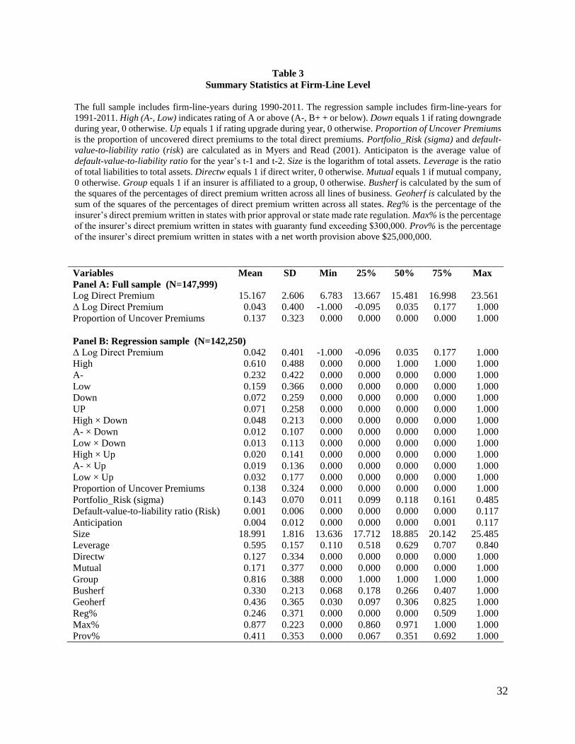
32

Table 3

Summary Statistics at Firm-Line Level

The full sample includes firm-line-years during 1990-2011. The regression sample includes firm-line-years for

1991-2011. High (A-, Low) indicates rating of A or above (A-, B+ + or below). Down equals 1 if rating downgrade

during year, 0 otherwise. Up equals 1 if rating upgrade during year, 0 otherwise. Proportion of Uncover Premiums

is the proportion of uncovered direct premiums to the total direct premiums. Portfolio_Risk (sigma) and default-

value-to-liability ratio (risk) are calculated as in Myers and Read (2001). Anticipaton is the average value of

default-value-to-liability ratio for the year’s t-1 and t-2. Size is the logarithm of total assets. Leverage is the ratio

of total liabilities to total assets. Directw equals 1 if direct writer, 0 otherwise. Mutual equals 1 if mutual company,

0 otherwise. Group equals 1 if an insurer is affiliated to a group, 0 otherwise. Busherf is calculated by the sum of

the squares of the percentages of direct premium written across all lines of business. Geoherf is calculated by the

sum of the squares of the percentages of direct premium written across all states. Reg% is the percentage of the

insurer’s direct premium written in states with prior approval or state made rate regulation. Max% is the percentage

of the insurer’s direct premium written in states with guaranty fund exceeding $300,000. Prov% is the percentage

of the insurer’s direct premium written in states with a net worth provision above $25,000,000.

Variables Mean SD Min 25% 50% 75% Max

Panel A: Full sample (N=147,999)

Log Direct Premium 15.167 2.606 6.783 13.667 15.481 16.998 23.561

Δ Log Direct Premium 0.043 0.400 -1.000 -0.095 0.035 0.177 1.000

Proportion of Uncover Premiums 0.137 0.323 0.000 0.000 0.000 0.000 1.000

Panel B: Regression sample (N=142,250)

Δ Log Direct Premium 0.042 0.401 -1.000 -0.096 0.035 0.177 1.000

High 0.610 0.488 0.000 0.000 1.000 1.000 1.000

A- 0.232 0.422 0.000 0.000 0.000 0.000 1.000

Low 0.159 0.366 0.000 0.000 0.000 0.000 1.000

Down 0.072 0.259 0.000 0.000 0.000 0.000 1.000

UP 0.071 0.258 0.000 0.000 0.000 0.000 1.000

High × Down 0.048 0.213 0.000 0.000 0.000 0.000 1.000

A- × Down 0.012 0.107 0.000 0.000 0.000 0.000 1.000

Low × Down 0.013 0.113 0.000 0.000 0.000 0.000 1.000

High × Up 0.020 0.141 0.000 0.000 0.000 0.000 1.000

A- × Up 0.019 0.136 0.000 0.000 0.000 0.000 1.000

Low × Up 0.032 0.177 0.000 0.000 0.000 0.000 1.000

Proportion of Uncover Premiums 0.138 0.324 0.000 0.000 0.000 0.000 1.000

Portfolio_Risk (sigma) 0.143 0.070 0.011 0.099 0.118 0.161 0.485

Default-value-to-liability ratio (Risk) 0.001 0.006 0.000 0.000 0.000 0.000 0.117

Anticipation 0.004 0.012 0.000 0.000 0.000 0.001 0.117

Size 18.991 1.816 13.636 17.712 18.885 20.142 25.485

Leverage 0.595 0.157 0.110 0.518 0.629 0.707 0.840

Directw 0.127 0.334 0.000 0.000 0.000 0.000 1.000

Mutual 0.171 0.377 0.000 0.000 0.000 0.000 1.000

Group 0.816 0.388 0.000 1.000 1.000 1.000 1.000

Busherf 0.330 0.213 0.068 0.178 0.266 0.407 1.000

Geoherf 0.436 0.365 0.030 0.097 0.306 0.825 1.000

Reg% 0.246 0.371 0.000 0.000 0.000 0.509 1.000

Max% 0.877 0.223 0.000 0.860 0.971 1.000 1.000

Prov% 0.411 0.353 0.000 0.067 0.351 0.692 1.000

33

Table 4

Number and Percentage of Sample Firm-line-years, by Rating Categories

Panel A:

Uncovered Rating

No. of

observation

%

Total No change

% No

change Upgrade

%

Upgrade Downgrade

%

Downgrade

High A++ 2335 10.07% 2142 91.73% 0 0.00% 193 8.27%

A+ 6266 27.03% 5544 88.48% 217 3.46% 505 8.06%

A 7448 32.13% 6626 88.96% 373 5.01% 449 6.03%

Total 16049 69.24% 14312 89.18% 590 3.68% 1147 7.15%

A- 5049 21.78% 4322 85.60% 498 9.86% 229 4.54%

Low B++ 878 3.79% 604 68.79% 204 23.24% 70 7.97%

B+ 801 3.46% 492 61.42% 262 32.71% 45 5.62%

B 257 1.11% 170 66.15% 69 26.85% 18 7.00%

B- 80 0.35% 47 58.75% 27 33.75% 6 7.50%

C++ 17 0.07% 5 29.41% 9 52.94% 3 17.65%

C+ 31 0.13% 13 41.94% 17 54.84% 1 3.23%

C 16 0.07% 10 62.50% 6 37.50% 0 0.00%

C- 1 0.00% 0 0.00% 0 0.00% 1 100.00%

Total 2081 8.98% 1341 64.44% 594 28.54% 144 6.92%

Total 23179 100.00% 19975 86.18% 1682 7.26% 1520 6.56%

Panel B:

Covered Rating

No. of

observation

%

Total No change

% No

change Upgrade

%

Upgrade Downgrade

%

Downgrade

High A++ 7704 6.17% 6979 90.59% 0 0.00% 725 9.41%

A+ 29294 23.47% 26019 88.82% 773 2.64% 2502 8.54%

A 37832 30.31% 33649 88.94% 1536 4.06% 2647 7.00%

Total 74830 59.95% 66647 89.06% 2309 3.09% 5874 7.85%

A- 28606 22.92% 24878 86.97% 2259 7.90% 1469 5.14%

Low B++ 8097 6.49% 6240 77.07% 1215 15.01% 642 7.93%

B+ 7657 6.13% 5446 71.12% 1594 20.82% 616 8.05%

B 3416 2.74% 2422 70.90% 720 21.08% 274 8.02%

B- 1274 1.02% 791 62.09% 358 28.10% 125 9.81%

C++ 362 0.29% 205 56.63% 127 35.08% 30 8.29%

C+ 320 0.26% 154 48.13% 131 40.94% 35 10.94%

C 217 0.17% 113 52.07% 97 44.70% 7 3.23%

C- 41 0.03% 27 65.85% 12 29.27% 2 4.88%

Total 21384 17.13% 15398 72.01% 4254 19.89% 1731 8.09%

Total 124820 100.00% 106923 85.66% 8822 7.07% 9074 7.27%

34

Table 5

Mean and Median Abnormal Premium Growth at Firm-Line-Years, 1990-2011

Table 5 shows the adjusted mean (median) abnormal premium growth rate for downgrades and upgrades. The uncovered-group is defined as firm-line-years with

a proportion of uncovered premiums greater than or equal to 25%. The covered-group is defined as firm-line-years with a proportion of uncovered premiums less

than 25%. Time, line, and size adjusted mean [median] abnormal premium growth in year t equals the firm-line-year’s premium growth in year t minus the mean

[median] time, line, and size adjusted premium growth in year t for firm-line-years with no rating change in year t. Medians are reported in square parentheses.

Significance of tests of differences in means are based on a two-tailed t-test and the difference in medians are based on a two-sided nonparametric Wilcoxon rank

sum test. The one-tailed t-test standard error are reported in parentheses. Bold values are significant at the 5% level.

Downgrades Upgrades

t-1 t t+1 t-1 t t+1

Uncovered group -1.67%

(0.02)

[-1.50%]

-13.50%

(0.02)

[-8.36%]

-10.03%

(0.02)

[-2.60%]

Uncovered group -5.46%

(0.02)

[-1.95%]

4.38%

(0.02)

[3.53%]

3.72%

(0.02)

[4.14%]

19975 no change; 1520 downgrades 19975 no change; 1682 upgrades

Covered group -2.42%

(0.01)

[-1.13%]

-7.52%

(0.01)

[-4.70%]

-7.77%

(0.01)

[-3.62%]

Covered group -2.89%

(0.01)

[-1.23%]

-0.33%

(0.01)

[0.37%]

1.81%

(0.01)

[0.98%]

106923 no change; 9074 downgrades 106923 no change; 8822 upgrades

Mean difference 0.76% -5.73% -2.26% Mean difference -2.57% 4.71% 1.91%

Median difference 0.37% -3.66% 1.02% Median difference -0.72% 3.16% 3.16%

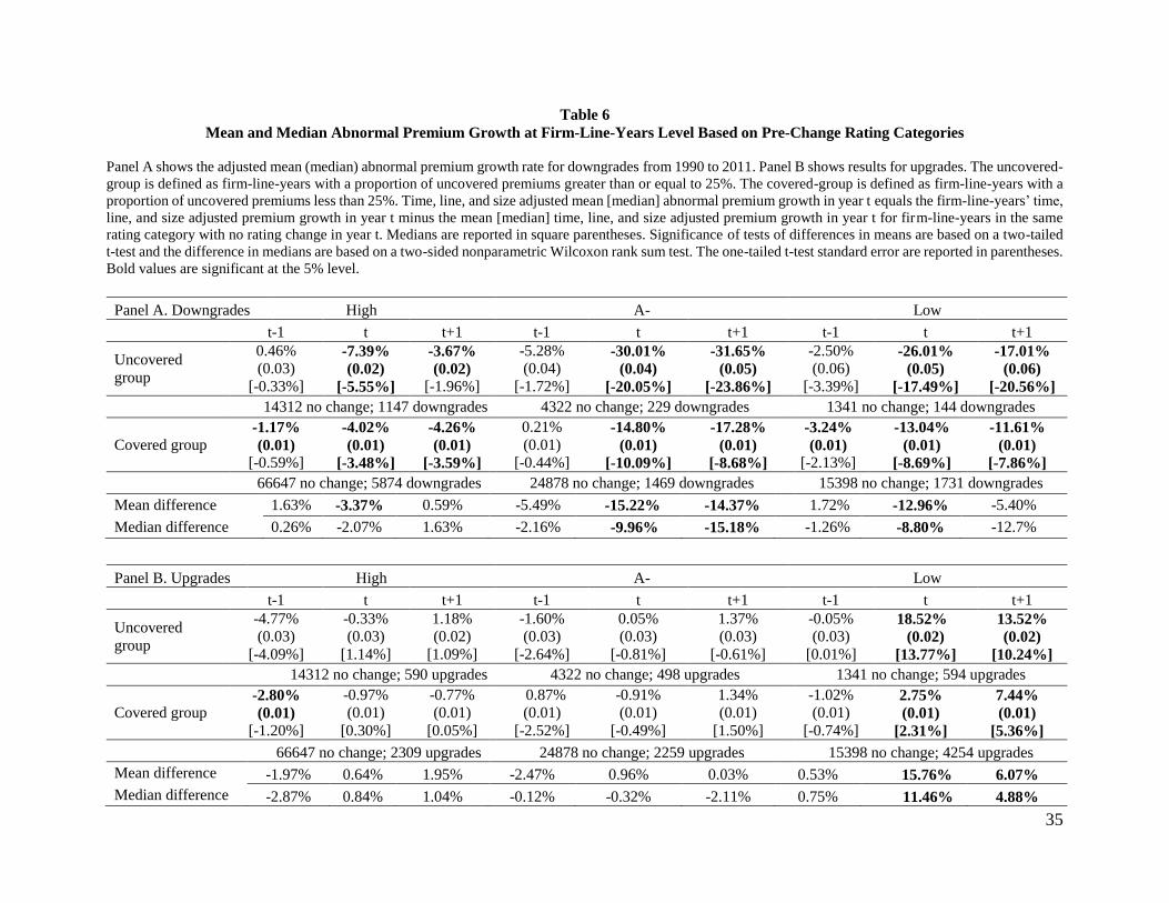
35

Table 6

Mean and Median Abnormal Premium Growth at Firm-Line-Years Level Based on Pre-Change Rating Categories

Panel A shows the adjusted mean (median) abnormal premium growth rate for downgrades from 1990 to 2011. Panel B shows results for upgrades. The uncovered-

group is defined as firm-line-years with a proportion of uncovered premiums greater than or equal to 25%. The covered-group is defined as firm-line-years with a

proportion of uncovered premiums less than 25%. Time, line, and size adjusted mean [median] abnormal premium growth in year t equals the firm-line-years’ time,

line, and size adjusted premium growth in year t minus the mean [median] time, line, and size adjusted premium growth in year t for firm-line-years in the same

rating category with no rating change in year t. Medians are reported in square parentheses. Significance of tests of differences in means are based on a two-tailed

t-test and the difference in medians are based on a two-sided nonparametric Wilcoxon rank sum test. The one-tailed t-test standard error are reported in parentheses.

Bold values are significant at the 5% level.

Panel A. Downgrades High A- Low

t-1 t t+1 t-1 t t+1 t-1 t t+1

Uncovered

group

0.46%

(0.03)

[-0.33%]

-7.39%

(0.02)

[-5.55%]

-3.67%

(0.02)

[-1.96%]

-5.28%

(0.04)

[-1.72%]

-30.01%

(0.04)

[-20.05%]

-31.65%

(0.05)

[-23.86%]

-2.50%

(0.06)

[-3.39%]

-26.01%

(0.05)

[-17.49%]

-17.01%

(0.06)

[-20.56%]

14312 no change; 1147 downgrades 4322 no change; 229 downgrades 1341 no change; 144 downgrades

Covered group -1.17%

(0.01) [-0.59%]

-4.02%

(0.01)

[-3.48%]

-4.26%

(0.01)

[-3.59%]

0.21%

(0.01)

[-0.44%]

-14.80%

(0.01)

[-10.09%]

-17.28%

(0.01)

[-8.68%]

-3.24%

(0.01) [-2.13%]

-13.04%

(0.01)

[-8.69%]

-11.61%

(0.01)

[-7.86%]

66647 no change; 5874 downgrades 24878 no change; 1469 downgrades 15398 no change; 1731 downgrades

Mean difference 1.63% -3.37% 0.59% -5.49% -15.22% -14.37% 1.72% -12.96% -5.40%

Median difference 0.26% -2.07% 1.63% -2.16% -9.96% -15.18% -1.26% -8.80% -12.7%

Panel B. Upgrades High A- Low

t-1 t t+1 t-1 t t+1 t-1 t t+1

Uncovered

group

-4.77%

(0.03)

[-4.09%]

-0.33%

(0.03)

[1.14%]

1.18%

(0.02)

[1.09%]

-1.60%

(0.03)

[-2.64%]

0.05%

(0.03)

[-0.81%]

1.37%

(0.03)

[-0.61%]

-0.05%

(0.03)

[0.01%]

18.52%

(0.02)

[13.77%]

13.52%

(0.02)

[10.24%]

14312 no change; 590 upgrades 4322 no change; 498 upgrades 1341 no change; 594 upgrades

Covered group -2.80%

(0.01)

[-1.20%]

-0.97%

(0.01)

[0.30%]

-0.77%

(0.01)

[0.05%]

0.87%

(0.01)

[-2.52%]

-0.91%

(0.01)

[-0.49%]

1.34%

(0.01)

[1.50%]

-1.02%

(0.01)

[-0.74%]

2.75%

(0.01)

[2.31%]

7.44%

(0.01)

[5.36%]

66647 no change; 2309 upgrades 24878 no change; 2259 upgrades 15398 no change; 4254 upgrades

Mean difference -1.97% 0.64% 1.95% -2.47% 0.96% 0.03% 0.53% 15.76% 6.07%

Median difference -2.87% 0.84% 1.04% -0.12% -0.32% -2.11% 0.75% 11.46% 4.88%

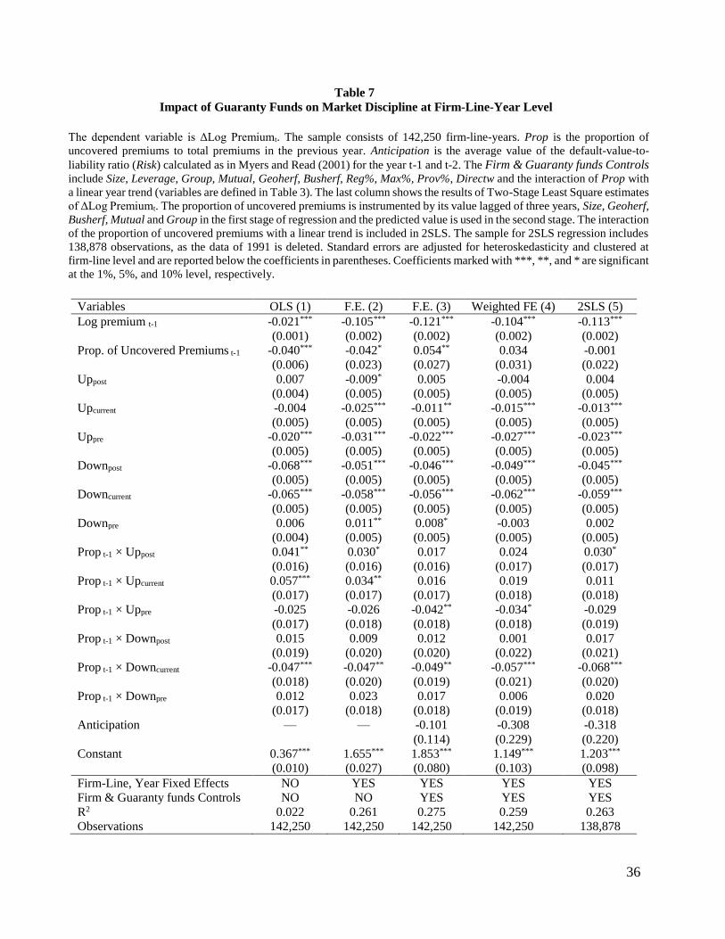
36

Table 7

Impact of Guaranty Funds on Market Discipline at Firm-Line-Year Level

The dependent variable is ΔLog Premiumt. The sample consists of 142,250 firm-line-years. Prop is the proportion of

uncovered premiums to total premiums in the previous year. Anticipation is the average value of the default-value-to-

liability ratio (Risk) calculated as in Myers and Read (2001) for the year t-1 and t-2. The Firm & Guaranty funds Controls

include Size, Leverage, Group, Mutual, Geoherf, Busherf, Reg%, Max%, Prov%, Directw and the interaction of Prop with

a linear year trend (variables are defined in Table 3). The last column shows the results of Two-Stage Least Square estimates

of ΔLog Premiumt. The proportion of uncovered premiums is instrumented by its value lagged of three years, Size, Geoherf,

Busherf, Mutual and Group in the first stage of regression and the predicted value is used in the second stage. The interaction

of the proportion of uncovered premiums with a linear trend is included in 2SLS. The sample for 2SLS regression includes

138,878 observations, as the data of 1991 is deleted. Standard errors are adjusted for heteroskedasticity and clustered at

firm-line level and are reported below the coefficients in parentheses. Coefficients marked with ***, **, and * are significant

at the 1%, 5%, and 10% level, respectively.

Variables OLS (1) F.E. (2) F.E. (3) Weighted FE (4) 2SLS (5)

Log premium t-1 -0.021*** -0.105*** -0.121*** -0.104*** -0.113***

(0.001) (0.002) (0.002) (0.002) (0.002)

Prop. of Uncovered Premiums t-1 -0.040*** -0.042* 0.054** 0.034 -0.001

(0.006) (0.023) (0.027) (0.031) (0.022)

Uppost 0.007 -0.009* 0.005 -0.004 0.004

(0.004) (0.005) (0.005) (0.005) (0.005)

Upcurrent -0.004 -0.025*** -0.011** -0.015*** -0.013***

(0.005) (0.005) (0.005) (0.005) (0.005)

Uppre -0.020*** -0.031*** -0.022*** -0.027*** -0.023***

(0.005) (0.005) (0.005) (0.005) (0.005)

Downpost -0.068*** -0.051*** -0.046*** -0.049*** -0.045***

(0.005) (0.005) (0.005) (0.005) (0.005)

Downcurrent -0.065*** -0.058*** -0.056*** -0.062*** -0.059***

(0.005) (0.005) (0.005) (0.005) (0.005)

Downpre 0.006 0.011** 0.008* -0.003 0.002

(0.004) (0.005) (0.005) (0.005) (0.005)

Prop t-1 × Uppost 0.041** 0.030* 0.017 0.024 0.030*

(0.016) (0.016) (0.016) (0.017) (0.017)

Prop t-1 × Upcurrent 0.057*** 0.034** 0.016 0.019 0.011

(0.017) (0.017) (0.017) (0.018) (0.018)

Prop t-1 × Uppre -0.025 -0.026 -0.042** -0.034* -0.029

(0.017) (0.018) (0.018) (0.018) (0.019)

Prop t-1 × Downpost 0.015 0.009 0.012 0.001 0.017

(0.019) (0.020) (0.020) (0.022) (0.021)

Prop t-1 × Downcurrent -0.047*** -0.047** -0.049** -0.057*** -0.068***

(0.018) (0.020) (0.019) (0.021) (0.020)

Prop t-1 × Downpre 0.012 0.023 0.017 0.006 0.020

(0.017) (0.018) (0.018) (0.019) (0.018)

Anticipation — — -0.101 -0.308 -0.318

(0.114) (0.229) (0.220)

Constant 0.367*** 1.655*** 1.853*** 1.149*** 1.203***

(0.010) (0.027) (0.080) (0.103) (0.098)

Firm-Line, Year Fixed Effects NO YES YES YES YES

Firm & Guaranty funds Controls NO NO YES YES YES

R2 0.022 0.261 0.275 0.259 0.263

Observations 142,250 142,250 142,250 142,250 138,878

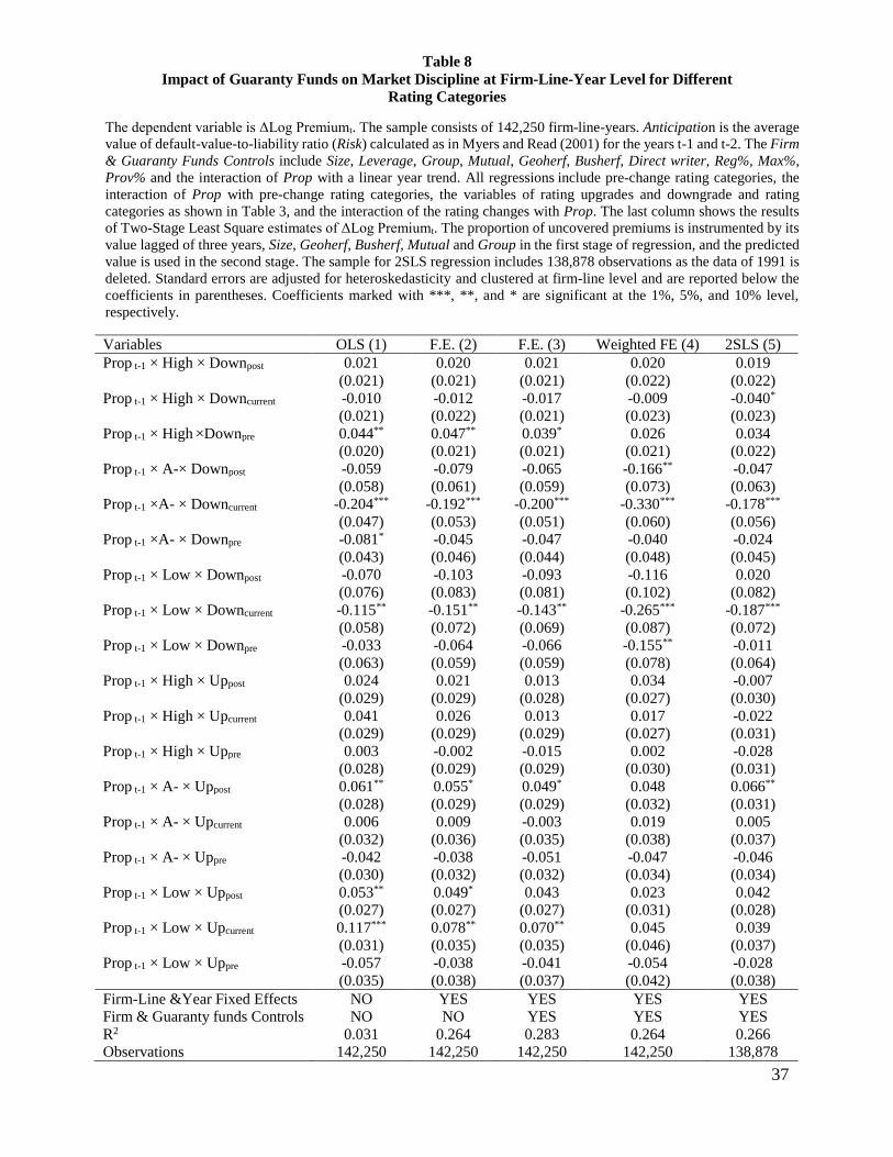
37

Table 8

Impact of Guaranty Funds on Market Discipline at Firm-Line-Year Level for Different

Rating Categories

The dependent variable is ΔLog Premiumt. The sample consists of 142,250 firm-line-years. Anticipation is the average

value of default-value-to-liability ratio (Risk) calculated as in Myers and Read (2001) for the years t-1 and t-2. The Firm

& Guaranty Funds Controls include Size, Leverage, Group, Mutual, Geoherf, Busherf, Direct writer, Reg%, Max%,

Prov% and the interaction of Prop with a linear year trend. All regressions include pre-change rating categories, the

interaction of Prop with pre-change rating categories, the variables of rating upgrades and downgrade and rating

categories as shown in Table 3, and the interaction of the rating changes with Prop. The last column shows the results

of Two-Stage Least Square estimates of ΔLog Premiumt. The proportion of uncovered premiums is instrumented by its

value lagged of three years, Size, Geoherf, Busherf, Mutual and Group in the first stage of regression, and the predicted

value is used in the second stage. The sample for 2SLS regression includes 138,878 observations as the data of 1991 is

deleted. Standard errors are adjusted for heteroskedasticity and clustered at firm-line level and are reported below the

coefficients in parentheses. Coefficients marked with ***, **, and * are significant at the 1%, 5%, and 10% level,

respectively.

Variables OLS (1) F.E. (2) F.E. (3) Weighted FE (4) 2SLS (5)

Prop t-1 × High × Downpost 0.021 0.020 0.021 0.020 0.019

(0.021) (0.021) (0.021) (0.022) (0.022)

Prop t-1 × High × Downcurrent -0.010 -0.012 -0.017 -0.009 -0.040*

(0.021) (0.022) (0.021) (0.023) (0.023)

Prop t-1 × High ×Downpre 0.044** 0.047** 0.039* 0.026 0.034

(0.020) (0.021) (0.021) (0.021) (0.022)

Prop t-1 × A-× Downpost -0.059 -0.079 -0.065 -0.166** -0.047

(0.058) (0.061) (0.059) (0.073) (0.063)

Prop t-1 ×A- × Downcurrent -0.204*** -0.192*** -0.200*** -0.330*** -0.178***

(0.047) (0.053) (0.051) (0.060) (0.056)

Prop t-1 ×A- × Downpre -0.081* -0.045 -0.047 -0.040 -0.024

(0.043) (0.046) (0.044) (0.048) (0.045)

Prop t-1 × Low × Downpost -0.070 -0.103 -0.093 -0.116 0.020

(0.076) (0.083) (0.081) (0.102) (0.082)

Prop t-1 × Low × Downcurrent -0.115** -0.151** -0.143** -0.265*** -0.187***

(0.058) (0.072) (0.069) (0.087) (0.072)

Prop t-1 × Low × Downpre -0.033 -0.064 -0.066 -0.155** -0.011

(0.063) (0.059) (0.059) (0.078) (0.064)

Prop t-1 × High × Uppost 0.024 0.021 0.013 0.034 -0.007

(0.029) (0.029) (0.028) (0.027) (0.030)

Prop t-1 × High × Upcurrent 0.041 0.026 0.013 0.017 -0.022

(0.029) (0.029) (0.029) (0.027) (0.031)

Prop t-1 × High × Uppre 0.003 -0.002 -0.015 0.002 -0.028

(0.028) (0.029) (0.029) (0.030) (0.031)

Prop t-1 × A- × Uppost 0.061** 0.055* 0.049* 0.048 0.066**

(0.028) (0.029) (0.029) (0.032) (0.031)

Prop t-1 × A- × Upcurrent 0.006 0.009 -0.003 0.019 0.005

(0.032) (0.036) (0.035) (0.038) (0.037)

Prop t-1 × A- × Uppre -0.042 -0.038 -0.051 -0.047 -0.046

(0.030) (0.032) (0.032) (0.034) (0.034)

Prop t-1 × Low × Uppost 0.053** 0.049* 0.043 0.023 0.042

(0.027) (0.027) (0.027) (0.031) (0.028)

Prop t-1 × Low × Upcurrent 0.117*** 0.078** 0.070** 0.045 0.039

(0.031) (0.035) (0.035) (0.046) (0.037)

Prop t-1 × Low × Uppre -0.057 -0.038 -0.041 -0.054 -0.028

(0.035) (0.038) (0.037) (0.042) (0.038)

Firm-Line &Year Fixed Effects NO YES YES YES YES Firm & Guaranty funds Controls NO NO YES YES YES

R2 0.031 0.264 0.283 0.264 0.266

Observations 142,250 142,250 142,250 142,250 138,878

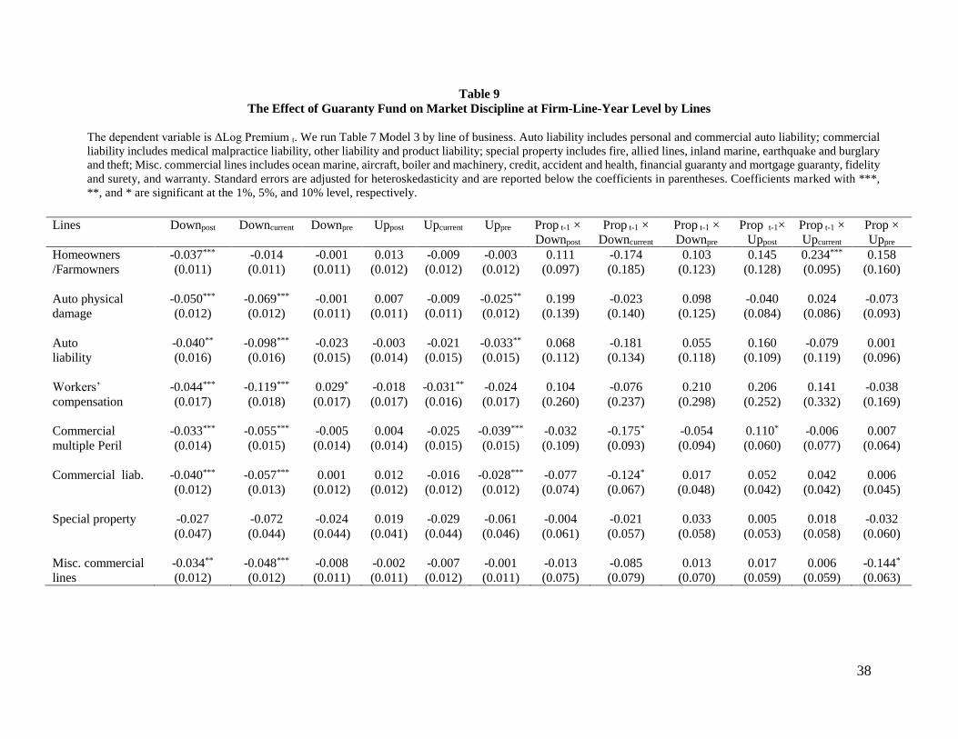
38

Table 9

The Effect of Guaranty Fund on Market Discipline at Firm-Line-Year Level by Lines

The dependent variable is ΔLog Premium t. We run Table 7 Model 3 by line of business. Auto liability includes personal and commercial auto liability; commercial

liability includes medical malpractice liability, other liability and product liability; special property includes fire, allied lines, inland marine, earthquake and burglary

and theft; Misc. commercial lines includes ocean marine, aircraft, boiler and machinery, credit, accident and health, financial guaranty and mortgage guaranty, fidelity

and surety, and warranty. Standard errors are adjusted for heteroskedasticity and are reported below the coefficients in parentheses. Coefficients marked with ***,

**, and * are significant at the 1%, 5%, and 10% level, respectively.

Lines Downpost Downcurrent Downpre Uppost Upcurrent Uppre Prop t-1 ×

Downpost

Prop t-1 ×

Downcurrent

Prop t-1 ×

Downpre

Prop t-1×

Uppost

Prop t-1 ×

Upcurrent

Prop ×

Uppre

Homeowners -0.037*** -0.014 -0.001 0.013 -0.009 -0.003 0.111 -0.174 0.103 0.145 0.234*** 0.158

/Farmowners (0.011) (0.011) (0.011) (0.012) (0.012) (0.012) (0.097) (0.185) (0.123) (0.128) (0.095) (0.160)

Auto physical -0.050*** -0.069*** -0.001 0.007 -0.009 -0.025** 0.199 -0.023 0.098 -0.040 0.024 -0.073

damage (0.012) (0.012) (0.011) (0.011) (0.011) (0.012) (0.139) (0.140) (0.125) (0.084) (0.086) (0.093)

Auto -0.040** -0.098*** -0.023 -0.003 -0.021 -0.033** 0.068 -0.181 0.055 0.160 -0.079 0.001

liability (0.016) (0.016) (0.015) (0.014) (0.015) (0.015) (0.112) (0.134) (0.118) (0.109) (0.119) (0.096)

Workers’ -0.044*** -0.119*** 0.029* -0.018 -0.031** -0.024 0.104 -0.076 0.210 0.206 0.141 -0.038

compensation (0.017) (0.018) (0.017) (0.017) (0.016) (0.017) (0.260) (0.237) (0.298) (0.252) (0.332) (0.169)

Commercial -0.033*** -0.055*** -0.005 0.004 -0.025 -0.039*** -0.032 -0.175* -0.054 0.110* -0.006 0.007

multiple Peril (0.014) (0.015) (0.014) (0.014) (0.015) (0.015) (0.109) (0.093) (0.094) (0.060) (0.077) (0.064)

Commercial liab. -0.040*** -0.057*** 0.001 0.012 -0.016 -0.028*** -0.077 -0.124* 0.017 0.052 0.042 0.006

(0.012) (0.013) (0.012) (0.012) (0.012) (0.012) (0.074) (0.067) (0.048) (0.042) (0.042) (0.045)

Special property -0.027 -0.072 -0.024 0.019 -0.029 -0.061 -0.004 -0.021 0.033 0.005 0.018 -0.032

(0.047) (0.044) (0.044) (0.041) (0.044) (0.046) (0.061) (0.057) (0.058) (0.053) (0.058) (0.060)

Misc. commercial -0.034** -0.048*** -0.008 -0.002 -0.007 -0.001 -0.013 -0.085 0.013 0.017 0.006 -0.144*

lines (0.012) (0.012) (0.011) (0.011) (0.012) (0.011) (0.075) (0.079) (0.070) (0.059) (0.059) (0.063)

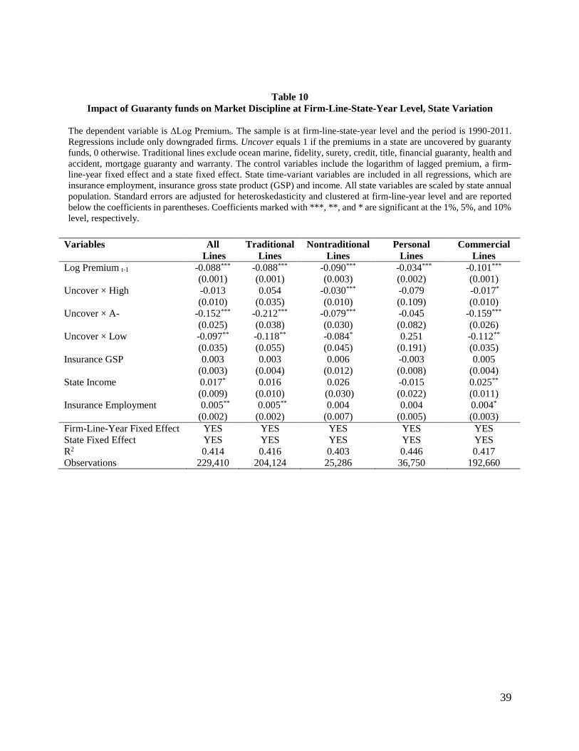
39

Table 10

Impact of Guaranty funds on Market Discipline at Firm-Line-State-Year Level, State Variation

The dependent variable is ΔLog Premiumt. The sample is at firm-line-state-year level and the period is 1990-2011.

Regressions include only downgraded firms. Uncover equals 1 if the premiums in a state are uncovered by guaranty

funds, 0 otherwise. Traditional lines exclude ocean marine, fidelity, surety, credit, title, financial guaranty, health and

accident, mortgage guaranty and warranty. The control variables include the logarithm of lagged premium, a firm-

line-year fixed effect and a state fixed effect. State time-variant variables are included in all regressions, which are

insurance employment, insurance gross state product (GSP) and income. All state variables are scaled by state annual

population. Standard errors are adjusted for heteroskedasticity and clustered at firm-line-year level and are reported

below the coefficients in parentheses. Coefficients marked with ***, **, and * are significant at the 1%, 5%, and 10%

level, respectively.

Variables All

Lines

Traditional

Lines

Nontraditional

Lines

Personal

Lines

Commercial

Lines

Log Premium t-1 -0.088***

(0.001)

-0.088***

(0.001)

-0.090***

(0.003)

-0.034***

(0.002)

-0.101***

(0.001)

Uncover × High -0.013

(0.010)

0.054

(0.035)

-0.030***

(0.010)

-0.079

(0.109)

-0.017*

(0.010)

Uncover × A- -0.152***

(0.025)

-0.212***

(0.038)

-0.079***

(0.030)

-0.045

(0.082)

-0.159***

(0.026)

Uncover × Low -0.097**

(0.035)

-0.118**

(0.055)

-0.084*

(0.045)

0.251

(0.191)

-0.112**

(0.035)

Insurance GSP 0.003

(0.003)

0.003

(0.004)

0.006

(0.012)

-0.003

(0.008)

0.005

(0.004)

State Income 0.017*

(0.009)

0.016

(0.010)

0.026

(0.030)

-0.015

(0.022)

0.025**

(0.011)

Insurance Employment 0.005**

(0.002)

0.005**

(0.002)

0.004

(0.007)

0.004

(0.005)

0.004*

(0.003)

Firm-Line-Year Fixed Effect YES YES YES YES YES

State Fixed Effect YES YES YES YES YES

R2 0.414 0.416 0.403 0.446 0.417

Observations 229,410 204,124 25,286 36,750 192,660

40

Table 11

Impact of Guaranty funds on Market Discipline at Firm-Line-State-Year Level, Line of Business variation

The dependent variable is ΔLog Premiumt. The sample is at firm-line-state-year level and the period is 1990-2011.

Regressions include only downgraded firms. Uncover equals 1 if the premiums in a state are uncovered by guaranty

funds, 0 otherwise. Traditional lines exclude ocean marine, fidelity, surety, credit, title, financial guaranty, health and

accident, mortgage guaranty and warranty. The set of control variables include logarithm of lagged premium, a firm-

state-year fixed effect and an insurance line of business fixed effect. Aggregate line of business time-variant variables

are included in all regressions, which are loss ratio and loss volatility. Standard errors are adjusted for

heteroskedasticity and clustered at firm-state-year level and are reported below the coefficients in parentheses.

Coefficients marked with ***, **, and * are significant at the 1%, 5%, and 10% level, respectively.

Variables All lines Nontraditional Lines Commercial Lines

Log Premium t-1 -0.059***

(0.001)

-0.037***

(0.004)

-0.070***

(0.001)

Uncover × High -0.058***

(0.011)

-0.028

(0.026)

-0.064***

(0.011)

Uncover × A- -0.053**

(0.021)

-0.264*

(0.133)

-0.044**

(0.022)

Uncover × Low -0.055*

(0.032)

-0.174

(0.155)

-0.059*

(0.032)

Loss Ratio -0.007

(0.011)

-0.336**

(0.140)

0.002

(0.011)

Loss Volatility 0.007

(0.008)

0.196**

(0.091)

-0.003

(0.008)

Firm-State-Year Fixed Effect YES YES YES

Line Fixed Effect YES YES YES

R2 0.427 0.726 0.447

Observations 229,410 25,286 192,660

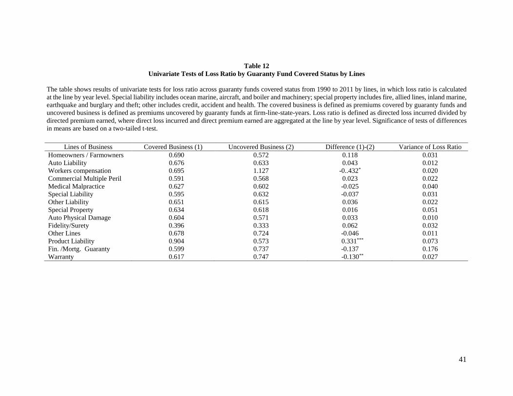
41

Table 12

Univariate Tests of Loss Ratio by Guaranty Fund Covered Status by Lines

The table shows results of univariate tests for loss ratio across guaranty funds covered status from 1990 to 2011 by lines, in which loss ratio is calculated

at the line by year level. Special liability includes ocean marine, aircraft, and boiler and machinery; special property includes fire, allied lines, inland marine,

earthquake and burglary and theft; other includes credit, accident and health. The covered business is defined as premiums covered by guaranty funds and

uncovered business is defined as premiums uncovered by guaranty funds at firm-line-state-years. Loss ratio is defined as directed loss incurred divided by

directed premium earned, where direct loss incurred and direct premium earned are aggregated at the line by year level. Significance of tests of differences

in means are based on a two-tailed t-test.

Lines of Business Covered Business (1) Uncovered Business (2) Difference (1)-(2) Variance of Loss Ratio

Homeowners / Farmowners 0.690 0.572 0.118 0.031

Auto Liability 0.676 0.633 0.043 0.012

Workers compensation 0.695 1.127 -0..432* 0.020

Commercial Multiple Peril 0.591 0.568 0.023 0.022

Medical Malpractice 0.627 0.602 -0.025 0.040

Special Liability 0.595 0.632 -0.037 0.031

Other Liability 0.651 0.615 0.036 0.022

Special Property 0.634 0.618 0.016 0.051

Auto Physical Damage 0.604 0.571 0.033 0.010

Fidelity/Surety 0.396 0.333 0.062 0.032

Other Lines 0.678 0.724 -0.046 0.011

Product Liability 0.904 0.573 0.331*** 0.073

Fin. /Mortg. Guaranty 0.599 0.737 -0.137 0.176

Warranty 0.617 0.747 -0.130** 0.027

42

Table 13 Insurers’ Risk Management Behavior

The dependent variable is ΔLog Premiumt. The sample period is 1991-2011. Risky business is defined as the first

seven insurance lines with high variances of loss ratio based on Table 12. Regressions include only business

covered by guaranty funds. In Panel A, the sample is at firm-year level. The sample consists of 33,104 firm-years.

Firm controls are included in the regression, which are Size, Leverage, Group, Mutual, Geoherf, Busherf, Directw, Anticipation and the interaction of Prop Risk with a linear year trend (variables are defined in Table 3). Prop Risk

is defined as the proportion of direct premiums written in risky business to total premiums written in a firm.

Standard errors are adjusted for heteroskedasticity and clustered at firm level and are reported below the

coefficients in parentheses. In Panel B, the sample is at firm-line-state-year level. Regressions include only firms

with a ratings downgrade. Risk equals 1 if the premiums are in a line which is risky business, 0 otherwise. The set

of control variables include logarithm of lagged premium, firm-year, state and insurance line of business fixed

effects. Standard errors are adjusted for heteroskedasticity and clustered at firm-year level and are reported below

the coefficients in parentheses. Coefficients marked with ***, **, and * are significant at the 1%, 5%, and 10%

level, respectively.

Panel A: Variables Firm-Year

Level

Log premium t-1 -0.108***

(0.005)

Prop. Risk -0.110***

(0.041)

Uppost 0.008

(0.011)

Upcurrent 0.001

(0.011)

Uppre -0.018*

(0.011)

Downpost -0.051***

(0.013)

Downcurrent -0.074***

(0.013)

Downpre -0.004

(0.012)

Prop Risk× Uppost -0.003

(0.021)

Prop Risk × Upcurrent -0.012

(0.024)

Prop Risk × Uppre -0.014

(0.024)

Prop Risk × Downpost 0.002

(0.026)

Prop Risk × Downcurrent 0.038

(0.026)

Prop Risk × Downpre 0.003

(0.025)

Firm, Year Fixed Effect YES

R2 0.250

Observations 33,104

Panel B: Variables Firm-Year-Line-State

Level

Log Premium t-1 -0.054***

(0.002)

Risky business × High -0.055

(0.057)

Risky business × A- -0.035

(0.061)

Risky business × Low 0.018

(0.060)

Firm-Year Fixed Effect YES

Line Fixed Effect YES

State Fixed Effect YES

R2 0.427

Observations 198,468

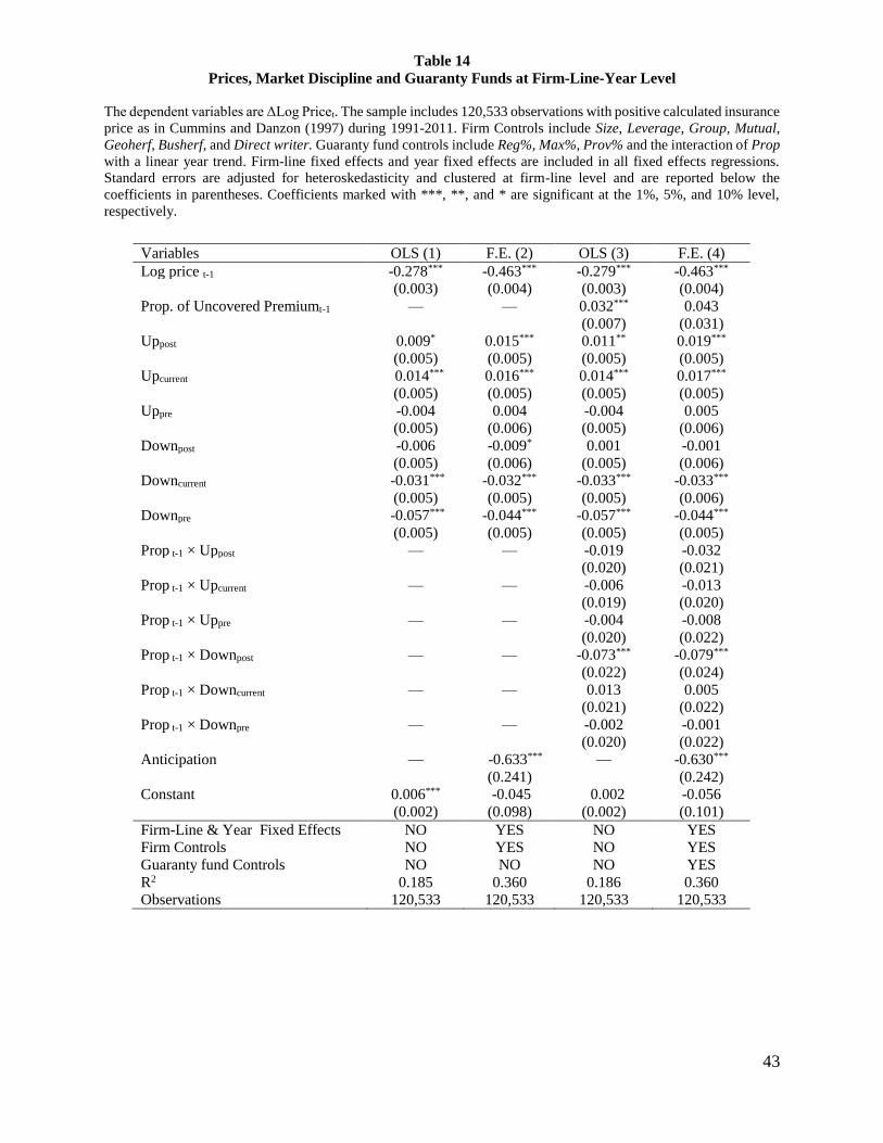
43

Table 14

Prices, Market Discipline and Guaranty Funds at Firm-Line-Year Level

The dependent variables are ΔLog Pricet. The sample includes 120,533 observations with positive calculated insurance

price as in Cummins and Danzon (1997) during 1991-2011. Firm Controls include Size, Leverage, Group, Mutual,

Geoherf, Busherf, and Direct writer. Guaranty fund controls include Reg%, Max%, Prov% and the interaction of Prop

with a linear year trend. Firm-line fixed effects and year fixed effects are included in all fixed effects regressions.

Standard errors are adjusted for heteroskedasticity and clustered at firm-line level and are reported below the

coefficients in parentheses. Coefficients marked with ***, **, and * are significant at the 1%, 5%, and 10% level,

respectively.

Variables OLS (1) F.E. (2) OLS (3) F.E. (4)

Log price t-1 -0.278*** -0.463*** -0.279*** -0.463***

(0.003) (0.004) (0.003) (0.004)

Prop. of Uncovered Premiumt-1 — — 0.032*** 0.043

(0.007) (0.031)

Uppost 0.009* 0.015*** 0.011** 0.019***

(0.005) (0.005) (0.005) (0.005)

Upcurrent 0.014*** 0.016*** 0.014*** 0.017***

(0.005) (0.005) (0.005) (0.005)

Uppre -0.004 0.004 -0.004 0.005

(0.005) (0.006) (0.005) (0.006)

Downpost -0.006 -0.009* 0.001 -0.001

(0.005) (0.006) (0.005) (0.006)

Downcurrent -0.031*** -0.032*** -0.033*** -0.033***

(0.005) (0.005) (0.005) (0.006)

Downpre -0.057*** -0.044*** -0.057*** -0.044***

(0.005) (0.005) (0.005) (0.005)

Prop t-1 × Uppost — — -0.019 -0.032

(0.020) (0.021)

Prop t-1 × Upcurrent — — -0.006 -0.013

(0.019) (0.020)

Prop t-1 × Uppre — — -0.004 -0.008

(0.020) (0.022)

Prop t-1 × Downpost — — -0.073*** -0.079***

(0.022) (0.024)

Prop t-1 × Downcurrent — — 0.013 0.005

(0.021) (0.022)

Prop t-1 × Downpre — — -0.002 -0.001

(0.020) (0.022)

Anticipation — -0.633*** — -0.630***

(0.241) (0.242)

Constant 0.006*** -0.045 0.002 -0.056

(0.002) (0.098) (0.002) (0.101)

Firm-Line & Year Fixed Effects NO YES NO YES

Firm Controls NO YES NO YES

Guaranty fund Controls NO NO NO YES

R2 0.185 0.360 0.186 0.360

Observations 120,533 120,533 120,533 120,533

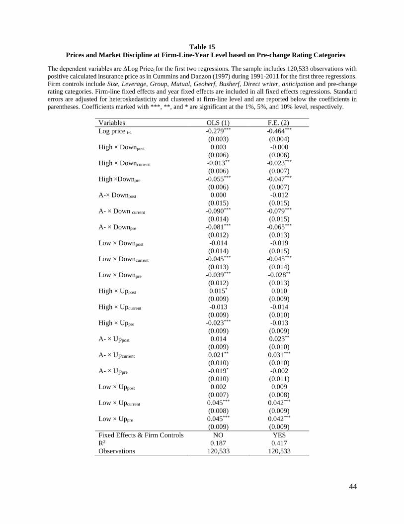
44

Table 15

Prices and Market Discipline at Firm-Line-Year Level based on Pre-change Rating Categories

The dependent variables are ΔLog Pricet for the first two regressions. The sample includes 120,533 observations with

positive calculated insurance price as in Cummins and Danzon (1997) during 1991-2011 for the first three regressions.

Firm controls include Size, Leverage, Group, Mutual, Geoherf, Busherf, Direct writer, anticipation and pre-change

rating categories. Firm-line fixed effects and year fixed effects are included in all fixed effects regressions. Standard

errors are adjusted for heteroskedasticity and clustered at firm-line level and are reported below the coefficients in

parentheses. Coefficients marked with ***, **, and * are significant at the 1%, 5%, and 10% level, respectively.

Variables OLS (1) F.E. (2)

Log price t-1 -0.279*** -0.464***

(0.003) (0.004)

High × Downpost 0.003 -0.000

(0.006) (0.006)

High × Downcurrent -0.013** -0.023***

(0.006) (0.007)

High ×Downpre -0.055*** -0.047***

(0.006) (0.007)

A-× Downpost 0.000 -0.012

(0.015) (0.015)

A- × Down current -0.090*** -0.079***

(0.014) (0.015)

A- × Downpre -0.081*** -0.065***

(0.012) (0.013)

Low × Downpost -0.014 -0.019

(0.014) (0.015)

Low × Downcurrent -0.045*** -0.045***

(0.013) (0.014)

Low × Downpre -0.039*** -0.028**

(0.012) (0.013)

High × Uppost 0.015* 0.010

(0.009) (0.009)

High × Upcurrent -0.013 -0.014

(0.009) (0.010)

High × Uppre -0.023*** -0.013

(0.009) (0.009)

A- × Uppost 0.014 0.023**

(0.009) (0.010)

A- × Upcurrent 0.021** 0.031***

(0.010) (0.010)

A- × Uppre -0.019* -0.002

(0.010) (0.011)

Low × Uppost 0.002 0.009

(0.007) (0.008)

Low × Upcurrent 0.045*** 0.042***

(0.008) (0.009)

Low × Uppre 0.045*** 0.042***

(0.009) (0.009)

Fixed Effects & Firm Controls NO YES

R2 0.187 0.417

Observations 120,533 120,533

45

Table 16

Prices, Market Discipline and Guaranty Funds at Firm-Line-Year Level based on Pre-change Rating

Categories

The dependent variable is ΔLog Pricet for the first three regressions. The sample period is 1991-2011. The sample

consists of 120,533 observations with positive calculated insurance price. Fixed effects and Controls include firm-line

fixed effects, year fixed effects, Size, Group, Mutual, Geoherf, Busherf, Direct writer, Anticipation, Reg%, Max%,

and Prov% and the interaction of Prop with a linear year trend. All regressions include upgrades, downgrades, pre-

change rating categories, the interactions of rating change and pre-rating categories, and the interaction of Prop with

pre-change rating categories. The third regression column shows the results of Two-Stage Least Square estimates of

ΔLog Pricet. The proportion of uncovered premiums is instrumented by its value lagged of three years, Size, Geoherf,

Busherf, Mutual and Group in the first stage of the 2SLS regression. The sample for the 2SLS regression includes

118,539 since the data of 1991 is deleted. Standard errors are adjusted for heteroskedasticity and clustered at firm-line

level and are reported below the coefficients in parentheses. Coefficients marked with ***, **, and * are significant

at the 1%, 5%, and 10% level, respectively.

Variables OLS (1) F.E. (2) 2SLS (3)

Prop t-1 × High × Downpost -0.074*** -0.073*** -0.074*** (0.024) (0.027) (0.027)

Prop t-1 × High × Downcurrent 0.013 0.015 0.014 (0.023) (0.026) (0.027)

Prop t-1 × High ×Downpre -0.013 -0.005 -0.001 (0.023) (0.025) (0.027)

Prop t-1 × A-× Downpost -0.037 -0.043 -0.045 (0.066) (0.071) (0.073)

Prop t-1 ×A- × Downcurrent -0.065 -0.098* -0.110* (0.054) (0.056) (0.059)

Prop t-1 ×A- × Downpre -0.021 0.001 -0.001 (0.054) (0.057) (0.058)

Prop t-1 × Low × Downpost -0.146* -0.172 -0.170 (0.080) (0.107) (0.110)

Prop t-1 × Low × Downcurrent 0.067 0.038 0.099 (0.077) (0.086) (0.087)

Prop t-1 × Low × Downpre 0.107* 0.023 0.003 (0.065) (0.078) (0.077)

Prop t-1 × High × Uppost -0.063** -0.072** -0.083** (0.031) (0.033) (0.036)

Prop t-1 × High × Upcurrent 0.055* 0.028 0.040 (0.031) (0.032) (0.034)

Prop t-1 × High × Uppre 0.028 0.007 0.014 (0.031) (0.033) (0.035)

Prop t-1 × A- × Uppost -0.052 -0.036 -0.037 (0.035) (0.036) (0.038)

Prop t-1 × A- × Upcurrent -0.112*** -0.061 -0.062 (0.034) (0.038) (0.041)

Prop t-1 × A- × Uppre -0.014 0.034 0.028 (0.035) (0.039) (0.041)

Prop t-1 × Low × Uppost 0.044 0.012 0.019 (0.033) (0.035) (0.037)

Prop t-1 × Low × Upcurrent 0.052 0.051 0.033 (0.038) (0.047) (0.050)

Prop t-1 × Low × Uppre 0.000 -0.030 -0.063 (0.040) (0.047) (0.049) Fixed effects and Controls NO YES YES

R2 0.187 0.361 0.358

Observations 120,533 120,533 118,539

46

Table 17

Market Discipline and Guaranty Funds at Firm-Line-Year Level after Controlling for Price

The dependent variables are ΔLog Premium t for the regressions. The 2SLS regression uses predicted price growth,

which is instrumented by lagged log price, rating vectors and firm and guaranty funds controls in the first stage. The

sample period is 1991-2011. The sample consists of 120,533 observations with positive calculated insurance price.

All regressions include upgrades, downgrades, pre-change rating categories, firm controls, and firm-line and year

fixed effects. The second model also include Prop, guaranty fund controls, the interactions of rating change and pre-

rating categories, the interaction of Prop with pre-change rating categories, and the interaction of Prop with a linear

year trend. Firm controls include Size, Group, Mutual, Geoherf, Busherf, Direct writer, Anticipation, Reg%; and

guaranty funds controls include Max%, and Prov%. Standard errors are adjusted for heteroskedasticity and clustered

at firm-line level and are reported below the coefficients in parentheses. Coefficients marked with ***, **, and * are

significant at the 1%, 5%, and 10% level, respectively.

Variables 2SLS (1) Variables 2SLS (2)

Predicted ΔLog Price t -0.043*** Predicted ΔLog Price t -0.071***

(0.002) (0.004)

High × Downpost -0.018*** Prop t-1 × High × Downpost 0.010

(0.005) (0.016)

High × Downcurrent -0.030*** Prop t-1 × High × Downcurrent -0.001

(0.005) (0.015)

High ×Downpre -0.002 Prop t-1× High ×Downpre 0.018

(0.005) (0.015)

A-× Downpost -0.057*** Prop t-1 × A-× Downpost -0.054

(0.010) (0.042)

A- × Down current -0.120*** Prop t-1×A- × Downcurrent -0.178***

(0.009) (0.035)

A- × Downpre 0.003 Prop t-1 ×A- × Downpre -0.002

(0.009) (0.035)

Low × Downpost -0.075*** Prop t-1 × Low × Downpost -0.025

(0.010) (0.054)

Low × Downcurrent -0.081*** Prop t-1 × Low × Downcurrent -0.181***

(0.009) (0.047)

Low × Downpre 0.009 Prop t-1 × Low × Downpre -0.052

(0.009) (0.045)

High × Uppost -0.022*** Prop t-1 × High × Uppost -0.004

(0.007) (0.020)

High × Upcurrent -0.020*** Prop t-1 × High × Upcurrent 0.026

0.007 (0.020)

High × Uppre -0.027*** Prop t-1 × High × Uppre -0.016

(0.007 (0.021)

A- × Uppost -0.007 Prop t-1 × A- × Uppost 0.060***

(0.007) (0.022)

A- × Upcurrent -0.012 Prop t-1 × A- × Upcurrent -0.022

(0.007) (0.023)

A- × Uppre -0.009 Prop t-1 × A- × Uppre -0.012

(0.007) (0.024)

Low × Uppost 0.030*** Prop t-1 × Low × Uppost -0.024

(0.006) (0.022)

Low × Upcurrent 0.039*** Prop t-1 × Low × Upcurrent 0.026

(0.006) (0.027)

Low × Uppre 0.009 Prop t-1 × Low × Uppre -0.036

(0.007) (0.029)

R2 0.126 R2 0.124

Observations 120,533 Observations 120,533

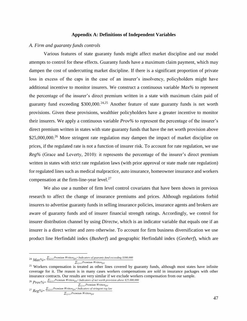
47

Appendix A: Definitions of Independent Variables

A. Firm and guaranty funds controls

Various features of state guaranty funds might affect market discipline and our model

attempts to control for these effects. Guaranty funds have a maximum claim payment, which may

dampen the cost of undercutting market discipline. If there is a significant proportion of private

loss in excess of the caps in the case of an insurer’s insolvency, policyholders might have

additional incentive to monitor insurers. We construct a continuous variable Max% to represent

the percentage of the insurer’s direct premium written in a state with maximum claim paid of

guaranty fund exceeding $300,000.24,25 Another feature of state guaranty funds is net worth

provisions. Given these provisions, wealthier policyholders have a greater incentive to monitor

their insurers. We apply a continuous variable Prov% to represent the percentage of the insurer’s

direct premium written in states with state guaranty funds that have the net worth provision above

$25,000,000.26 More stringent rate regulation may dampen the impact of market discipline on

prices, if the regulated rate is not a function of insurer risk. To account for rate regulation, we use

Reg% (Grace and Leverty, 2010): it represents the percentage of the insurer’s direct premium

written in states with strict rate regulation laws (with prior approval or state made rate regulation)

for regulated lines such as medical malpractice, auto insurance, homeowner insurance and workers

compensation at the firm-line-year level.27

We also use a number of firm level control covariates that have been shown in previous

research to affect the change of insurance premiums and prices. Although regulations forbid

insurers to advertise guaranty funds in selling insurance policies, insurance agents and brokers are

aware of guaranty funds and of insurer financial strength ratings. Accordingly, we control for

insurer distribution channel by using Directw, which is an indicator variable that equals one if an

insurer is a direct writer and zero otherwise. To account for firm business diversification we use

product line Herfindahl index (Busherf) and geographic Herfindahl index (Geoherf), which are

24 Max%=

∑ Premium Writtenijsti,j,s,t ×Indicators of guaranty fund exceeding $300,000

∑ Premium Writtenijsti,j,s,t

25 Workers compensation is treated as other lines covered by guaranty funds, although most states have infinite

coverage for it. The reason is in many cases workers compensations are sold in insurance packages with other

insurance contracts. Our results are very similar if we exclude workers compensation from our sample.

26 Prov%=∑ Premium Writtenijsti,j,s,t ×Indicators of net worth provision above $25,000,000

∑ Premium Writtenijsti,j,s,t

27 Reg%=∑ Premium Writtenijsti,j,s,t ×Indicators of stringent reg law

∑ Premium Writtenijsti,j,s,t

48

calculated by the sum of the squares of the percentages of direct premium written across all lines

of business (all states for geographic Herfindahl index) for the insurer. Other firm characteristic

control variables are Size, the natural logarithm of total assets; Leverage, the ratio of total liability

to total asset; Mutual, a dummy variable set equal to one if the insurer is a mutual organization;

and Group, an indicator if the firm belongs to some affiliated group.

B. Default-value-to-liability ratio

It is possible that insurers and markets anticipate the rating changes of some firms and thus

react less to the rating changes. To control for this possibility, we use a continuous measure of

insurer risk. Specifically, we calculate an insurer’s default-value-to-liability ratio (Risk) (Myers

and Read, 2001):

}{)1(}{),( zNszNsfd (A1)

where 𝑁{·} is the cumulative probability function for the standard normal variable, 𝑠 is the surplus

to liability ratio, 2log 1 / 2

 s

z

, and 𝜎 is the volatility of the asset to liability ratio. The

overall firm’s volatility of the asset to liability ratio is calculated as 2 2 2  V L VL , where

𝜎𝑉 is the volatility of insurer’s assets, σL is the volatility of insurer’s liabilities, and 𝜎𝑉𝐿 is the

covariance of the natural logarithms of liabilities and assets. The respective volatilities are

calculated by the following functions:

2   i j i j

M M

V i j VV V V

i j

x x (A2)

2    i j i j

N N

L i j L L L L

i j

y y (A3)

2  i j i j

M N

VL i j V L V L

i j

x y (A4)

where xi is the proportion of asset from asset type 𝑖 to total asset, yi is the proportion of liabilities

from line 𝑖 to the loss liability, ρViVj

is the correlation coefficient of the logarithms of asset classes

𝑖 and 𝑗 with 𝑀 number of asset classes28, ρLiLj

is the correlation coefficient of the logarithms of

28 Assets are divided into six classes: stocks, bonds, real estate, mortgages, cash and other invested, and other assets.

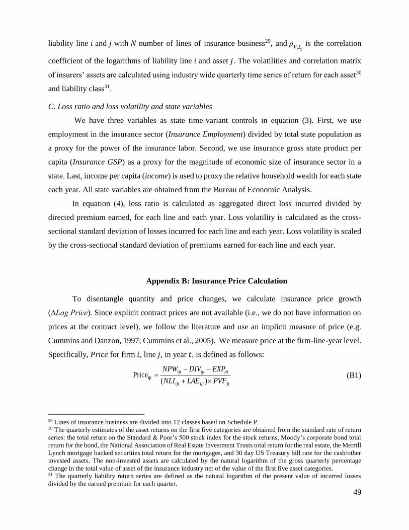
49

liability line 𝑖 and 𝑗 with 𝑁 number of lines of insurance business29, and ρViLj

is the correlation

coefficient of the logarithms of liability line 𝑖 and asset 𝑗. The volatilities and correlation matrix

of insurers’ assets are calculated using industry wide quarterly time series of return for each asset30

and liability class31.

C. Loss ratio and loss volatility and state variables

We have three variables as state time-variant controls in equation (3). First, we use

employment in the insurance sector (Insurance Employment) divided by total state population as

a proxy for the power of the insurance labor. Second, we use insurance gross state product per

capita (Insurance GSP) as a proxy for the magnitude of economic size of insurance sector in a

state. Last, income per capita (income) is used to proxy the relative household wealth for each state

each year. All state variables are obtained from the Bureau of Economic Analysis.

In equation (4), loss ratio is calculated as aggregated direct loss incurred divided by

directed premium earned, for each line and each year. Loss volatility is calculated as the cross-

sectional standard deviation of losses incurred for each line and each year. Loss volatility is scaled

by the cross-sectional standard deviation of premiums earned for each line and each year.

Appendix B: Insurance Price Calculation

To disentangle quantity and price changes, we calculate insurance price growth

(∆Log Price). Since explicit contract prices are not available (i.e., we do not have information on

prices at the contract level), we follow the literature and use an implicit measure of price (e.g.

Cummins and Danzon, 1997; Cummins et al., 2005). We measure price at the firm-line-year level.

Specifically, Price for firm 𝑖, line 𝑗, in year 𝑡, is defined as follows:

jtijtijt

ijtijtijt

PVFLAENLI

EXPDIVNPW

)(Priceijt (B1)

29 Lines of insurance business are divided into 12 classes based on Schedule P. 30 The quarterly estimates of the asset returns on the first five categories are obtained from the standard rate of return

series: the total return on the Standard & Poor’s 500 stock index for the stock returns, Moody’s corporate bond total

return for the bond, the National Association of Real Estate Investment Trusts total return for the real estate, the Merrill

Lynch mortgage backed securities total return for the mortgages, and 30 day US Treasury bill rate for the cash/other

invested assets. The non-invested assets are calculated by the natural logarithm of the gross quarterly percentage

change in the total value of asset of the insurance industry net of the value of the first five asset categories. 31 The quarterly liability return series are defined as the natural logarithm of the present value of incurred losses

divided by the earned premium for each quarter.

50

Where NPW is net premiums written, DIV is dividends to policyholders, EXP is underwriting

expenses, NLI is net losses incurred, LAE is loss adjustment expenses incurred, and PVF is the

present value factor for line j, in year t. Since premiums reflect the discounting of loss in a

competitive market, losses incurred and loss adjustment expenses are discounted using a present

value factor that accounts for differences in the payout pattern across insurance lines (e.g. long-

tail lines vs. short tail lines). To calculate present value factors (PVF) we use information about

how losses developed in the past to estimate how losses develop in the future. Specifically, we

estimate payout proportions for each insurance line by applying the Taylor separation method

(Taylor, 2002) to loss reserve data from the Schedule P of the regulatory annual statements.32 We

discount these estimated future payments using US Treasury yields obtained from the Federal

Reserve Bank of St Louis. The estimation of payout tail proportions is akin to the method

prescribed by the Internal Revenue Service (IRS) for computing loss present values for tax

purposes (Cummins 1990).

32 Schedule P of the NAIC regulatory annual statement aggregates each insurer’s lines of business into 12 categories:

homeowner/farmers, auto liability, commercial multiple peril, workers’ compensation, medical malpractice, special

liability (ocean marine, aircraft and boiler & machinery), other liability, special property (fire, allied lines, inland

marine, earthquake, burglary and theft), auto physical damages, fidelity/surety, other, and warranty.

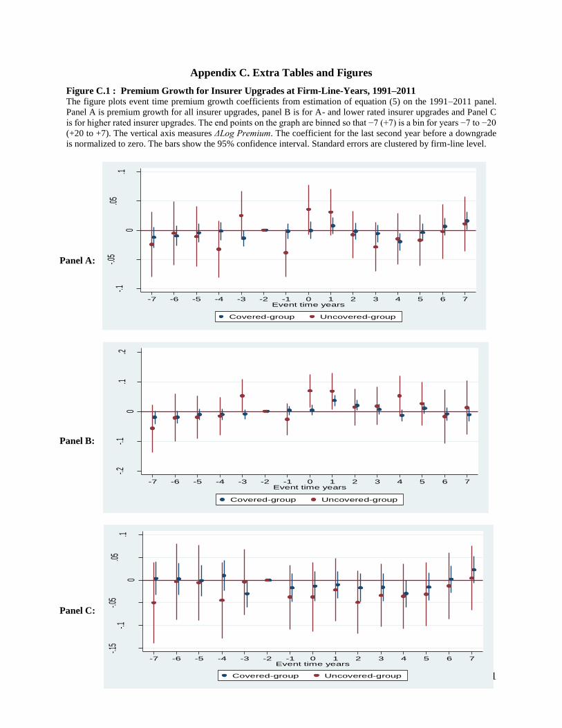
51

-.1-.0

5

0

.05

.1

Insu

ranc

e Pr

emiu

m G

rowt

h

-7 -6 -5 -4 -3 -2 -1 0 1 2 3 4 5 6 7Event time years

Covered-group Uncovered-group

-.2-.1

0.1

.2

Insu

ranc

e Pr

emiu

m G

rowt

h

-7 -6 -5 -4 -3 -2 -1 0 1 2 3 4 5 6 7Event time years

Covered-group Uncovered-group

-.15

-.1-.0

5

0

.05

.1

Insu

ranc

e Pr

emium

Gro

wth

-7 -6 -5 -4 -3 -2 -1 0 1 2 3 4 5 6 7Event time years

Covered-group Uncovered-group

Appendix C. Extra Tables and Figures

Figure C.1 : Premium Growth for Insurer Upgrades at Firm-Line-Years, 1991–2011 The figure plots event time premium growth coefficients from estimation of equation (5) on the 1991–2011 panel.

Panel A is premium growth for all insurer upgrades, panel B is for A- and lower rated insurer upgrades and Panel C

is for higher rated insurer upgrades. The end points on the graph are binned so that −7 (+7) is a bin for years −7 to −20

(+20 to +7). The vertical axis measures ΔLog Premium. The coefficient for the last second year before a downgrade

is normalized to zero. The bars show the 95% confidence interval. Standard errors are clustered by firm-line level.

Panel A:

Panel B:

Panel C:

52

Table C.1

Seemingly Unrelated Regression for Premium Growth and Price Growth The dependent variables are ΔLog Premiumt and ΔLog Pricet for the SUR regression. The sample includes 120,533

observations with positive calculated insurance price as in Cummins and Danzon (1997) during 1991-2011. Firm

controls, line fixed effects and year fixed effects are included in the regressions. Standard errors are adjusted for

heteroskedasticity and clustered at firm-line level and are reported below the coefficients in parentheses. Coefficients

marked with ***, **, and * are significant at the 1%, 5%, and 10% level, respectively.

F.E. (1) F.E. (2) Equality of

(ΔLog Premiumt) (ΔLog Pricet) Coefficients

High × Downpost -0.038*** 0.000 26.96***

(0.005) (0.006) (0.000)

High × Downcurrent -0.041*** -0.017*** 10.93***

(0.005) (0.006) (0.001)

High ×Downpre -0.007 -0.051*** 33.25***

(0.005) (0.006) (0.000)

A-× Downpost -0.087*** 0.005 31.54***

(0.010) (0.013) (0.000)

A- × Downcurrent -0.137*** -0.088*** 10.05***

(0.010) (0.012) (0.001)

A- × Downpre -0.005 -0.081*** 26.05***

(0.010) (0.012) (0.000)

Low × Downpost -0.095*** -0.016 23.56***

(0.010) (0.013) (0.000)

Low × Downcurrent -0.090*** -0.042*** 10.00***

(0.010) (0.012) (0.002)

Low × Downpre 0.030*** -0.031*** 16.33***

(0.010) (0.012) (0.000)

High × Uppost -0.008 0.020** 6.80

(0.007) (0.009) (0.009)

High × Upcurrent 0.004 -0.005 0.81

(0.007) (0.009) (0.369)

High × Uppre -0.006 -0.005 0.00

(0.007) (0.008) (0.998)

A- × Uppost -0.009 0.017* 4.85

(0.007) (0.009) (0.028)

A- × Upcurrent -0.004 0.030*** 8.04

(0.007) (0.009) (0.005)

A- × Uppre -0.008 -0.008 0.00

(0.008) (0.009) (0.964)

Low × Uppost 0.035*** 0.004 11.31***

(0.006) (0.007) (0.001)

Low × Upcurrent 0.053*** 0.050*** 0.13

(0.006) (0.008) (0.719)

Low × Uppre 0.022*** 0.049*** 6.65***

(0.007) (0.008) (0.010)

Fixed Effects & Firm Controls YES YES —

Observations 120,533 120,533 —

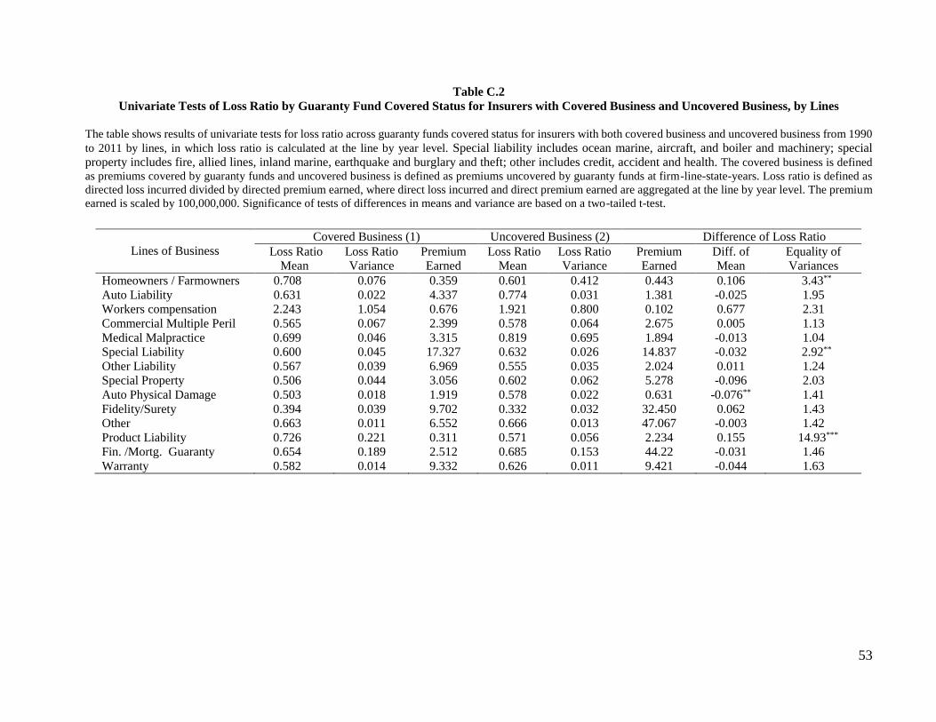
53

Table C.2

Univariate Tests of Loss Ratio by Guaranty Fund Covered Status for Insurers with Covered Business and Uncovered Business, by Lines

The table shows results of univariate tests for loss ratio across guaranty funds covered status for insurers with both covered business and uncovered business from 1990

to 2011 by lines, in which loss ratio is calculated at the line by year level. Special liability includes ocean marine, aircraft, and boiler and machinery; special

property includes fire, allied lines, inland marine, earthquake and burglary and theft; other includes credit, accident and health. The covered business is defined

as premiums covered by guaranty funds and uncovered business is defined as premiums uncovered by guaranty funds at firm-line-state-years. Loss ratio is defined as

directed loss incurred divided by directed premium earned, where direct loss incurred and direct premium earned are aggregated at the line by year level. The premium

earned is scaled by 100,000,000. Significance of tests of differences in means and variance are based on a two-tailed t-test.

Lines of Business

Covered Business (1) Uncovered Business (2) Difference of Loss Ratio

Loss Ratio

Mean

Loss Ratio

Variance

Premium

Earned

Loss Ratio

Mean

Loss Ratio

Variance

Premium

Earned

Diff. of

Mean

Equality of

Variances

Homeowners / Farmowners 0.708 0.076 0.359 0.601 0.412 0.443 0.106 3.43**

Auto Liability 0.631 0.022 4.337 0.774 0.031 1.381 -0.025 1.95

Workers compensation 2.243 1.054 0.676 1.921 0.800 0.102 0.677 2.31

Commercial Multiple Peril 0.565 0.067 2.399 0.578 0.064 2.675 0.005 1.13

Medical Malpractice 0.699 0.046 3.315 0.819 0.695 1.894 -0.013 1.04

Special Liability 0.600 0.045 17.327 0.632 0.026 14.837 -0.032 2.92**

Other Liability 0.567 0.039 6.969 0.555 0.035 2.024 0.011 1.24

Special Property 0.506 0.044 3.056 0.602 0.062 5.278 -0.096 2.03

Auto Physical Damage 0.503 0.018 1.919 0.578 0.022 0.631 -0.076** 1.41

Fidelity/Surety 0.394 0.039 9.702 0.332 0.032 32.450 0.062 1.43

Other 0.663 0.011 6.552 0.666 0.013 47.067 -0.003 1.42

Product Liability 0.726 0.221 0.311 0.571 0.056 2.234 0.155 14.93***

Fin. /Mortg. Guaranty 0.654 0.189 2.512 0.685 0.153 44.22 -0.031 1.46

Warranty 0.582 0.014 9.332 0.626 0.011 9.421 -0.044 1.63

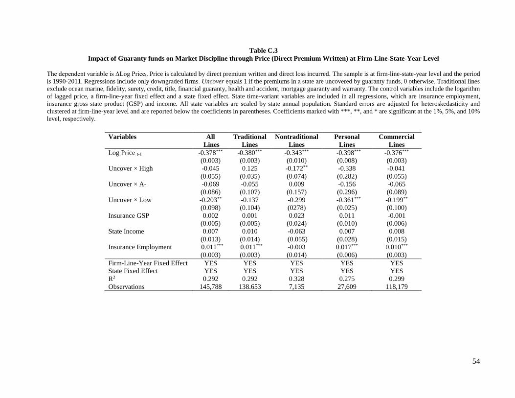
54

Table C.3

Impact of Guaranty funds on Market Discipline through Price (Direct Premium Written) at Firm-Line-State-Year Level

The dependent variable is ΔLog Pricet. Price is calculated by direct premium written and direct loss incurred. The sample is at firm-line-state-year level and the period

is 1990-2011. Regressions include only downgraded firms. Uncover equals 1 if the premiums in a state are uncovered by guaranty funds, 0 otherwise. Traditional lines

exclude ocean marine, fidelity, surety, credit, title, financial guaranty, health and accident, mortgage guaranty and warranty. The control variables include the logarithm

of lagged price, a firm-line-year fixed effect and a state fixed effect. State time-variant variables are included in all regressions, which are insurance employment,

insurance gross state product (GSP) and income. All state variables are scaled by state annual population. Standard errors are adjusted for heteroskedasticity and

clustered at firm-line-year level and are reported below the coefficients in parentheses. Coefficients marked with ***, **, and * are significant at the 1%, 5%, and 10%

level, respectively.

Variables All

Lines

Traditional

Lines

Nontraditional

Lines

Personal

Lines

Commercial

Lines

Log Price t-1 -0.378***

(0.003)

-0.380***

(0.003)

-0.343***

(0.010)

-0.398***

(0.008)

-0.376***

(0.003)

Uncover × High -0.045

(0.055)

0.125

(0.035)

-0.172**

(0.074)

-0.338

(0.282)

-0.041

(0.055)

Uncover × A- -0.069

(0.086)

-0.055

(0.107)

0.009

(0.157)

-0.156

(0.296)

-0.065

(0.089)

Uncover × Low -0.203**

(0.098)

-0.137

(0.104)

-0.299

(0278)

-0.361***

(0.025)

-0.199**

(0.100)

Insurance GSP 0.002

(0.005)

0.001

(0.005)

0.023

(0.024)

0.011

(0.010)

-0.001

(0.006)

State Income 0.007

(0.013)

0.010

(0.014)

-0.063

(0.055)

0.007

(0.028)

0.008

(0.015)

Insurance Employment 0.011***

(0.003)

0.011***

(0.003)

-0.003

(0.014)

0.017***

(0.006)

0.010***

(0.003)

Firm-Line-Year Fixed Effect YES YES YES YES YES

State Fixed Effect YES YES YES YES YES

R2 0.292 0.292 0.328 0.275 0.299

Observations 145,788 138.653 7,135 27,609 118,179