market evidence of misperceived prices and mistaken
TRANSCRIPT

Market Evidence of Misperceived Prices and Mistaken Mortality Risks JAYANTA BHATTACHARYA DANA P. GOLDMAN NEERAJ SOOD
WR-124
July 2003
National Institute on Aging

NBER WORKING PAPER SERIES
MARKET EVIDENCE OF MISPERCEIVED PRICESAND MISTAKEN MORTALITY RISKS
Jayanta BhattacharyaDana P. Goldman
Neeraj Sood
Working Paper 9863http://www.nber.org/papers/w9863
NATIONAL BUREAU OF ECONOMIC RESEARCH1050 Massachusetts Avenue
Cambridge, MA 02138July 2003
We are grateful to the National Institute on Aging for financial support. We thank Alan Garber, Victor Fuchs,William Vogt, Jim Dertouzos, Steve Garber, Ted Frech, Joe Newhouse, Matt Miller and seminar participantsat Stanford University, RAND, and UC Irvine for their comments. We especially thank Dan Kessler for aclose reading of and constructive comments on an earlier version of the paper. We are responsible for allremaining errors. Finally, we thank Dawn Matsui and Deborah Rivera for excellent editorial assistance. Theviews expressed herein are those of the authors and not necessarily those of the National Bureau of EconomicResearch
©2003 by Jayanta Bhattacharya, Dana P. Goldman, and Neeraj Sood. All rights reserved. Short sections oftext not to exceed two paragraphs, may be quoted without explicit permission provided that full creditincluding © notice, is given to the source.

Market Evidence of Misperceived Prices and Mistaken Mortality RisksJayanta Bhattacharya, Dana P. Goldman, and Neeraj SoodNBER Working Paper No. 9863July 2003JEL No. D8
ABSTRACT
This paper develops a market-based test of whether consumers make systematic mistakes in
assessing their own mortality risks, and whether they are able to make "correct" price comparisons
between insurance and credit markets. This test relies on data from secondary life insurance markets,
wherein consumers sell their life insurance policies to firms in return for an up front payment. We
find evidence consistent with the hypotheses that: (1) unhealthy consumers are systematically too
optimistic about their mortality risks and (2) consumers focus on nominal price information in
deciding to sell life insurance, rather than on the real discounted expected price.
Jay Bhattacharya Dana Goldman Neeraj SoodCenter for Primary Care RAND RANDand Outcomes Research 1700 Main Street 1700 Main StreetStanford Medical School Santa Monica, CA 90401 Santa Monica, CA 90401117 Encina Commons and NBER [email protected], CA 94305-6019 [email protected] [email protected]

1 Introduction
Making insurance and savings decisions is difficult. Traditional economicmodels of insurance decisions assume, at a minimum, that consumers cansolve two problems: (1) accurately assess the risks they face; and (2) inter-pret the information conveyed by market prices. But are these assumptionsreasonable, especially in markets where consumers face unfamiliar risks?
In this paper, we develop a market-based test of whether consumers makesystematic mistakes in assessing their own mortality risks, and whether theyare able to make ”correct” price comparisons between insurance and creditmarkets.1 Our test relies on new data from secondary life insurance markets,wherein consumers bequeath their life insurance policies to firms in returnfor an up-front payment. These markets are good candidates for such a testbecause they require consumers to assess risks regarding their own mortal-ity accurately, as well as decode complicated price signals in an unfamiliarenvironment.
To set up this test, we develop an economic model of the consumer deci-sion to sell life insurance in the secondary market in the context of compet-itive pricing.2 This model of a sophisticated consumer produces two sharppredictions. First, the model predicts a positive correlation between mortal-ity risk and the decision to sell life insurance. The reasoning is that a suddenincrease in mortality risk increases the consumers’ wealth by increasing themarket value of the consumers’ life insurance policy. In response to thisincrease in wealth, the consumers desire to increase both consumption andbequests. Thus consumers sell some or all of their life insurance policy anduse some of the proceeds for current consumption and invest the remainderfor future consumption or bequests. Second, the model predicts a positivecorrelation between asset holdings and the decision to sell life insurance.
Next, we contrast these predictions with the predictions from a modelwith two mutually consistent interpretations motivated by the psychologyand behavioral economics literature: that unhealthy consumers are system-atically too optimistic about their mortality risks and that consumers focuson nominal price information in deciding to sell insurance, rather than on thereal discounted expected price. This model also predicts a positive correla-tion between mortality and life insurance sales. However, in contrast to theeconomic model this model predicts that (1) among healthier patients thosewith significant non-liquid assets should be less likely to sell life insuranceand that (2) among sicker patients those with significant non-liquid assets
1

should be more likely to sell life insurance. We test predictions from thesemodels against data on life insurance sales by HIV+ consumers.
2 Literature Review
There are extensive literatures on both consumer perception of mortality riskand distortions in consumer decision-making under uncertainty. In this sec-tion we briefly summarize findings from both the psychology and the emerg-ing behavioral economics literature that are most relevant to our research.Barberis and Thaler [2002], Mullainathan and Thaler [2000], Kagel and Roth[1995], Rabin [1998], and Kahneman and Tversky [2000] provide deeper andmore extensive reviews.
In the past, the behavioral economics literature has typically relied ontwo types of non-market evidence: small-scale psychological experiments andconsumer self-reports of risk perceptions. Recently, market based tests of thepredictions of behavioral economics have emerged in two different settings:in financial markets [see Barberis and Thaler, 2002] and in the analysis ofconsumer savings behavior [see Bernheim et al., 1997].
2.1 Consumer perception of mortality risks
Extensive evidence from the psychology literature shows that people makesystematic mistakes in assessing their mortality risks. In particular, Lichten-stein et al. [1978] and several other studies have shown that people underes-timate mortality risks from likely causes of death and overestimate mortalityrisks from unlikely causes of death. In related research, studies have foundthat people overestimate highly publicized risks. For example, Moore andZhu [2000] hypothesize that given the recent flood of information on the al-leged hazards of passive smoking in government publications and the media,people are likely to overestimate the health risk of passive smoking. Theyfind evidence consistent with a model whereby individuals systematicallyoverestimate the effects of passive smoking on their health and where theshort-term effects of passive smoking on health care costs are negligible.
In addition to the evidence from psychology literature, recent studiesusing data on subjective survival expectations from the Health RetirementStudy (HRS) and the Asset and Health Dynamics Among the Oldest Old(AHEAD) find that people tend to be optimistic about their longevity, with ofoptimism greatest for people with the shortest life expectancies. Schoenbaum
2

[1997], using data from the HRS, shows that current heavy smokers tendto be overly optimistic about their probability of surviving to age 75; thatis, heavy smokers’ subjective assessment of their own survival probabilitiesare higher than those obtained from actuarial models. By contrast, neversmokers’ subjective assessment of their probability of surviving to age 75 ismarginally lower than the actuarial prediction.
Hurd et al. [1999] report a very similar pattern among older populationsusing data from the AHEAD. For example, 85-89 year-old female respon-dents’ subjective probability of surviving to age 100 years is 0.30, while thelife table value is merely 0.07. By contrast, preumably healthier 70-74 year-old female respondents are more pessimistic about their survival chances thanis warranted—their subjective probability of surviving to age 85 years is 0.51,while the life table value is 0.58.
The data from these studies show that peoples’ perceptions of their ownmortality risks are systematically biased. In particular, people with relativelylow life expectancy tend to underestimate their mortality risks and peoplewith relatively high life expectancy tend to marginally overestimate theirmortality risks.
2.2 Limits to consumer problem solving ability
While much of the literature on consumer perceptions of mortality risks hasfocused on consumer self-reports rather than market behavior, there is alsoa growing body of evidence from markets which suggests that consumershave limited information processing ability, and hence use simple heuristicsto economize on this scarce resource. Numerous studies have documentedhow these simple heuristics sometimes lead consumers to make systematicmistakes. For example, Odean [1998] finds that customers at a large broker-age firm were less likely to realize capital losses than capital gains despite taxincentives that encourage loss realization. Odean shows that this loss aver-sion is consistent with prospect theory [Kahneman and Tversky, 1979] andtheories of mental accounting [Thaler, 1985]. Similarly, Benartzi and Thaler[2001] find that individuals making asset allocation decisions in defined con-tribution plans use a naıve “1/n strategy”: they divide contributions evenlyacross the funds offered in the plans. Consistent with this naıve notion of di-versification they find that the proportion invested in stocks depends stronglyon the proportion of stock funds in the plan.
3

Bernheim et al. [1997] analyze household data on wealth and savings,arguing that the data are consistent with “rule of thumb” and “mental ac-counting” theories of wealth accumulation. They find little support for thetraditional life cycle model of savings and wealth accumulation. Laibson[1997] also analyzes household savings behavior and argues that people notonly find it difficult to make optimal savings decisions but often find it dif-ficult to stick their decisions. In particular, consumers’ short run discountrates are much higher than their long run discount rates, implying that pref-erences are time inconsistent. This discount structure leads consumers tosave little today even though savings are optimal from a life cycle perspec-tive. Liabson argues that consumers often invest in illiquid assets or othercommitment devices to overcome this tendency for over-consumption.
Finally, many standard textbooks on life insurance markets claim thatprice comparisons in life insurance are sufficiently complex to be well beyondthe analytic capabilities of “ordinary” consumers [Maclean, 1962; Magee,1958]. Research on life insurance markets reach similar conclusions. Forexample, Belth [1966] argues that the inability of consumers to make pricecomparisons in life insurance markets explains the persistence of substantialvariation in prices of similar life insurance products.
3 An Economic Model of the Decision to Sell Life In-
surance.
A secondary life insurance transaction (also called a viatical settlement) isthe sale of a life insurance policy to a third party for immediate cash paymentat a discount to face value; it involves the sale of a used life insurance policy.When a consumer sells his used policy, the buyer becomes the sole beneficiaryof the policy and she collects the face value of the policy when he dies.3
There is a good reason why this market attracts only consumers who havesuffered adverse health events. Life insurance premiums are set at the timeof purchase based upon the mortality profile of the consumer at the time ofpurchase. When the consumer suffers an adverse health event (worse thanaverage for his age), suddenly he is more likely to collect his life insuranceearlier than originally thought at the time of purchase. Indeed, his premiumswould be much higher were he to buy the policy after the event. In effect,the adverse health event creates equity in the consumer’s used life insurancepolicy. It is this equity, which is a real asset for the consumer, that is sold
4
on the viatical settlements market.With this reasoning in mind, we start our analysis of viatical settlement
markets by considering the plight of the chronically ill consumer who pur-chased life insurance prior to the development of illness. Consumers con-sidering whether to sell life insurance are often too frail to work—due tolife-threatening illness—and may need funds to finance consumption, includ-ing medical treatment. Though their liquid assets may be insufficient tosupport their consumption, these consumers have the option to sell or bor-row against their non-liquid assets, such as a house or life insurance, therebyreducing bequests.
3.1 A Model of Consumption and Bequests under Mortal Uncer-tainty
Consider a consumer whose initial wealth includes a house with a marketvalue of NL dollars (net of any outstanding loans against the house) and alife insurance policy with face value F dollars. In our simple model, thereare two periods: consumers survive the first period with certainty, die at thebeginning of the second period with probability π, and if they survive, diewith certainty at the end of the second period. Figure 1 is the timeline ofevents in this two-period model.
At the beginning of the first period the consumer earns income L1, sellsan amount F of his life insurance policy at the actuarially fair price, P (π),consumes an amount C1 and borrows or lends his remaining liquid assets. Atthe end of the first period the uncertainty about the length of the consumer’slife is resolved—he knows then whether he will survive to the second period.If the consumer dies he leaves assets BD as bequests in the beginning ofperiod two, consisting of the net value of the consumer’s house, proceeds ofhis remaining life insurance policy, and the portfolio of his bonds and interestpayments.
BD = (L1 + P (π) ∗ F − C1) ∗ (1 + r) + NL + F − F (1)
The first term in the parenthesis reflects the consumer’s net lending or bor-rowing.
If the consumer survives, then at the beginning of the second period,he earns income L2 and consumes an amount C2. Since all uncertainty isresolved by the beginning of the second period, we assume that the consumerbequeaths BS to his heirs and to the buyer of his life insurance policy at the
5

beginning of the second period rather than when he dies at the end of thesecond period. An heir who prefers to receive the bequest at the end of thesecond period can simply buy a bond of one-year maturity with his bequests.Under these conditions, second period bequests will include savings from thefirst period, life insurance that has not been cashed out, non-liquid assets,and unspent earnings from the second period:
BS = (L1 + P (π) ∗ F − C1)∗(1 + r)+(NL+F−F )∗(
1
1 + r
)+L2−C2 (2)
We assume that the market for used life insurance is competitive (seefootnote 2 for a justification of this assumption). Thus, P (π) is the perfectlycompetitive market price a viatical settlement company is willing to pay perunit face value of a policyholder with mortality risk π. Let r be the marketrate of interest at which the firms can borrow funds. Assuming that theconsumer continues to pay the premium on the policy even after the sale ofthe policy, the present value of the expected profit from the purchase of thepolicy is:
profits =
([π
1 + r+
1 − π
(1 + r)2
]− P (π)
)F (3)
The first terms in equation (3) represents the present value of the expectedrevenue the buyer would receive after the death of the policyholder, while thelast term represents the cost to the firm of purchasing the policy. Thereforethe zero-profit condition under perfect competition implies:
P (π) =
[π
1 + r+
1 − π
(1 + r)2
](4)
The above condition can be viewed as the demand for life insurance giventhe mortality risk of the consumer and the cost of funds for the firm. In equi-librium, the prices are actuarially fair and the firms are willing to buy alllife insurance policies supplied by consumers. The consumer’s problem is tochoose the optimal value of consumption and the financing of the consump-tion through sale of life insurance or credit to maximize expected utility fromconsumption and bequests.
EU = U (C1) + πβV (BD) + (1 − π) βU (C2) + (1 − π) βV (BS) (5)
6

Substituting equations (1), (2), and (4) for BD, BS, and P (π) respectively,and then differentiating (5) with respect to C1, C2, F yields the following firstorder conditions.
U ′ (C1)
[(π) V ′ (BD) + (1 − π)V ′ (BS)]= β (1 + r) (6)
U ′ (C2) = V ′ (BS) (7)
V ′ (BD) = V ′ (BS) (8)
Equation (6) shows that consumers choose consumption in the first pe-riod so that the ratio of the marginal utility of consumption to the expectedmarginal utility of bequests equals the ratio of the consumer’s intertemporaldiscount factor to the market discount factor. Similarly, equation (7) showsthat once the uncertainty about death is resolved, consumers choose con-sumption so that the marginal utility of consumption in the second periodequals the marginal utility of bequests in the second period.
Equation (8) shows that selling life insurance helps consumer reduce the“riskiness” of their bequest portfolio. As in other insurance markets, riskaverse consumers sell life insurance to equalize the marginal utility of be-quests whether the consumer dies at the end of the first period or survives tothe second period. Borrowing does not affect the “riskiness” of the bequestportfolio since the repayment of loans taken in prior periods is not contingenton the mortality of the consumer. On the other hand, selling life insuranceenables consumers to increase resources when alive at the cost of reducingnear term bequests. In other words, the ex post cost of obtaining funds froma viatical settlement (relative to borrowing) will depend on the timing of theconsumer’s death—if consumers die at the end of the second period then aviatical settlement will have lower costs than borrowing but if consumers dieat the end of the first period then viatical settlement will be more expensivethan borrowing. Of course, the expected ex ante cost of financing an extradollar of consumption through borrowing and selling life insurance will bethe same.
3.2 The Effect of Mortality Risk on the Size of the Settlement
Appendix A solves the consumer’s maximization problem and derives thekey comparative statics. The results show that an increase in mortality risk
7

increases the magnitude of life insurance sales.
dF
dπ> 0 (9)
The intuition for this result is as follows. An increase in mortality riskincreases the consumer’s wealth by increasing equity in the consumer’s lifeinsurance policy. In response to this increase in wealth, the consumer willdemand both increased consumption and bequests, which are both assumedto be normal goods. Thus the consumer will sell some or all of the lifeinsurance policy and use some of the proceeds for current consumption andinvest remaining proceeds for future consumption or bequests.
3.3 The Effect of Assets on the Size of the Settlement
The comparative static results show that an increase in the value of theconsumer’s house, or an increase in current income, raises the magnitude oflife insurance sales.
dF
dNL> 0 (10)
dF
dL1> 0 (11)
The intuition for these results is as follows. Trivially, an increase in thevalue of the consumer’s house or an increase in the current income increasesthe consumer’s wealth. This increase in wealth would mechanically increasethe size of near-term bequests, BD, were the consumer to die at the endof the first period. To maximize utility under these changed circumstancesand equate the marginal utility of bequests and consumption, the consumerwill want to liquidate some of his life insurance holdings, effectively movingfunds between from the early death state of the world (which is overly fundedbecause of the nature of the increased wealth) to the current time period.Therefore, the consumer will increase life insurance sales and use some of hiswealth to increase consumption and late term bequests, at the expense ofthe originally increased near term bequests.
In contrast, if the consumer experiences an increase in future income thenin equilibrium, he would reduce the magnitude of life insurance sales.
8
dF
dL2< 0 (12)
The intuition for this result is that an increase in future income increasesfuture bequests but leaves near term bequests unchanged. Consumers reducelife insurance sales and increase borrowing to simultaneously increase currentconsumption and bequests and reduce late-term bequests, again equilibratingmarginal utility across the states of the world and across time periods inaccordance with the first order conditions (6)-(8).
4 A Model of Misperceived Price and the Decision toSell Insurance
This section presents an alternative model of the decision to sell life insurancein which consumers have misperceptions about the real price (opportunitycost) of selling insurance. The key assumption in this model is that relativelyunhealthy consumers perceive a higher return from selling life insurance rel-ative to borrowing than actually exists, and that the opposite is true forrelatively healthy consumers. This assumption can be motivated in at leasttwo ways, both consistent with the spirit of the papers cited in our literaturereview.
The first motivation is that relatively unhealthy consumers overestimatetheir life expectancy while relatively healthy consumers slightly underesti-mate their life expectancy. This “optimism bias” of relatively unhealthyconsumers leads them to view actuarially fair viatical settlement offers morefavorably than they would appear to someone correctly perceiving mortalityrisk.
The second motivation is that consumers with limited analytic capabil-ities use a simple rule of thumb to calculate the present value of expectedcosts (in terms of forgone bequests) of a viatical settlement. In particular,consumers incorrectly mistake the discount to face value (nominal price) onthe viatical settlement for the true cost of a viatical settlement—which isthe net present value of foregone bequests. Since in competitive markets thediscount to face value rises with life expectancy this view also leads con-sumers to view actuarially fair viatical settlement offers more favorably ifthey expect to live a long life. For example, if viatical settlement firms face acost of borrowing of 15% per annum, then under a constant mortality hazard
9

assumption the actuarially fair price of a life insurance policy held by a con-sumer with life expectancy of 6 months is 95% (or 5% discount on face value)of the face value and for a consumer with a life expectancy of 2 years is 79%(or 21% discount on face value). We argue that consumers fixate on the dis-count to face value rather than the true cost (15% per annum) of the viaticalsettlement. Thus, consumers with life expectancy of 6 months prefer sellinglife insurance to borrowing at an interest rate of 15% per annum, and theopposite holds for consumers with life expectancy of 2 years. Even thoughprices are actuarially fair, unhealthy consumers prefer selling life insuranceand healthy consumers prefer borrowing.
As in the economic model of the previous section, consumers hold threedistinct assets: a life insurance policy, other non-liquid assets such as housing,and liquid assets such as income. They can finance consumption in threeways. They can consume liquid assets directly, borrow against other non-liquid assets at a given interest rate r, or sell part or all of their life insurancepolicy at a price p per dollar of coverage. Each action has costs in termsof foregone bequests. Liquid assets cannot be bequeathed once spent, loansmust be repaid, and heirs cannot collect on life insurance that has been sold.
Unlike in the economic model, consumers in this model solve a static opti-mization problem of distributing wealth between consumption and bequeststo maximize utility.4 In particular, such consumers do not discount bequests,while firms, which live forever and are risk neutral, discount future incomeat the market rate of interest. This simple model generates sharp predictionsthat we can test with the available data; adding some dynamic elements tothe model would complicate it without altering the main predictions that wetest in the empirical portion of the paper.
4.1 The Effect of Mortality Risk on the Size of the Settlement
As our example in the introduction to this section shows, the discount toface value of life insurance offered by viatical settlement firms depends on lifeexpectancy. Even for life insurance policies with the same face value, firmswill charge lower discounts to consumers closer the end of life since firmsare more likely to collect earlier. Since consumers in this section incorrectlyperceive the discount to face value as the true price of the viatical settlement,they trade off the discount to face value against the annual interest rate forborrowing. Assuming that the market interest rate for borrowing is the samefor everyone, relatively unhealthy consumers will perceive terms of trade to
10

be more lucrative in the viatical settlements market than in the credit market.More formally, let ai reflect consumer i’s risk of death, and let H1 =
{i|ai < a}, H2 = {i|ai = a}, and H3 = {i|ai > a} for some cutoff level a sothat H1 consists of healthier consumers than H3. We choose a cutoff valuea such that for consumers in H2, the perceived costs of financing currentconsumption through the credit and viatical settlement markets are equal.H1 consumers perceive lower prices in the credit market, while H3 consumersperceive the viatical settlements market to be more lucrative. Figure 2 showsthe budget constraint for H3 consumers. The vertical axis represents currentconsumption, the horizontal axis represents bequests, and W represents theinitial endowment,
(L, NL + F
). B represents the net present value of the
endowment—L + pF + NL1+r
, where p is the actuarially fair unit price of lifeinsurance sales.
Selling all of F moves consumers from W to A, where consumers have onlynon-liquid assets left to fund bequests. To increase current consumption pastA, consumers must turn to the credit market, where they borrow at interestrate r, represented by the line segment AB. At point B, consumers leaveno bequests, consuming everything in the current period. The kink in thebudget constraint is caused by consumer’s misperception about the relativeprices of borrowing and selling life insurance. A consumer who correctlyobserved that the real prices of the two activities are the same would havea straight line connecting points W and B for a budget constraint since thepolicy is discounted by firms at the market rate of interest, the same rate atwhich consumers can borrow.
Another strategy that consumers could pursue would be to borrow firstand then sell their life insurance after their credit is exhausted. WCB isthe perceived budget constraint for this strategy, where C represents theexhaustion of non-liquid asset collateral and B represents the sale of F as well.Since H3 (the unhealthiest) consumers perceive that the terms of trade favorthe viatical settlements market; the slope of WA is greater (in absolute value)than the slope of WC. Therefore, consumers will viaticate first and thenborrow only if pF is insufficient to finance current consumption. SimilarlyH1 (the healthiest) consumers will perceive that the terms of trade favorcredit markets and choose to borrow first. Therefore this model also predictsa negative correlation between health status and the decision to viaticate.
11

4.2 Effect of Assets on the Size of the Settlement
Changes in non-liquid assets lead to a parallel shift in the consumer’s bud-get line and do not affect the perceived terms of trade in the two markets.Increasing non-liquid assets raises both the value of the endowment and max-imum possible bequests, since consumers either leave additional non-liquidassets as bequests or use them for borrowing.
For healthy H1 consumers, these additional assets will induce them tosubstitute borrowing for life insurance sales, since the former is on more fa-vorable terms. Figure 3 shows this effect. H1 consumers initially borrow fullyagainst their non-liquid assets and also sell life insurance at E. For the utilitycurves as drawn, increasing NL shifts the budget line from WAB to W’A’B’.At E’, consumers have completely substituted borrowing for viaticating.5 Forother preferences, this complete substitution may not happen, but as long asconsumption and bequests are normal goods, increased assets will decreaselife insurance sales for H1 consumers.
For sicker H3 consumers, the additional non-liquid assets can induce morelife insurance sales. Figure 4 demonstrates the effect of an increase in NLfor H3 consumers. For these consumers, terms of trade favor the viaticalsettlements market. If consumption is a normal good, an increase in NLleads these consumers to sell a larger part of F , as they can use the additionalnon-liquid assets to finance bequests. At G’ on the new budget constraint,consumers sell the same amount of life insurance as at their initial optimum,E. Thus, the new equilibrium will lie on C’G’, where consumers sell a largerpart of F than at E.
Increasing liquid assets leads to a parallel shift in the consumer’s budgetconstraint. Consumers use additional liquid assets to either finance increasedconsumption or to increase bequests by substituting for viatication or bor-rowing. If bequests are a normal good, increasing liquid assets will causeconsumers to decrease their supply of life insurance, decrease their borrow-ing, or both. For H1 consumers who do not initially sell life insurance,increasing liquid assets will reduce borrowing but have no effect on life in-surance supply. For H3 consumers who sell all of their life insurance and alsoborrow, the effects of increasing L depend upon the strength of the incomeeffect. If the income effect is strong, consumers eliminate borrowing and re-duce their supply of life insurance. If the income effect is weak, consumerscontinue to sell all of F , but reduce borrowing. Hence, for H3 consumers aswell, increasing liquid assets will never increase the supply of life insurance.
12

5 Comparing Predictions from the Economic and Mis-perceived Price Model
Both the economic model and the misperceived price model make severalsharp predictions regarding the behavior of consumers in the viatical settle-ment and credit markets.
Prediction 1: Health status is negatively correlated with the decision toviaticate.
Although this prediction is consistent with both the economic model andthe misperceived price model the mechanism through which mortality risksaffect life insurance sales is very different across the two models. In theeconomic model an increase in mortality risk increases the value of the con-sumers’ life insurance policy. This “wealth-effect” induces consumers to in-crease life insurance sales to finance increased consumption at the cost ofreduced bequests. In contrast, in the misperceived price model the negativecorrelation between health status and the decision to viaticate arises froma “price-effect.” Unhealthy consumers perceive that the terms of trade aremore favorable in the viatical settlements market as the discount to face valueof their life insurance increases with life expectancy.
Prediction 2[E]: For all consumers, the decision to viaticate is positivelycorrelated with non-liquid assets.
This prediction is consistent with the economic model only and follows di-rectly from the comparative static result shown in equation (10). In contrast,the misperceived price model makes the following prediction:
Prediction 2[M]: For the healthiest consumers, the decision to viaticate isnegatively correlated with non-liquid assets. For the sickest, the decision toviaticate is positively correlated with non-liquid assets.
This follows from Figures 4 and 3 and is a rather stringent test of themisperceived price model. It requires that the impact of non-liquid assetson the decision to viaticate in our empirical specification have different signsdepending on the underlying health status of the consumer.
Prediction 3[E]: For all consumers, increase in liquid assets or current
13

income will increase the incentive to participate in the viatical settlementsmarket.
This prediction is consistent with the economic model only. Thus, itwould constitute evidence in favor of the economic model if we observe thatpeople with higher incomes are more likely to viaticate than are patients withlower incomes. In contrast, the misperceived price model makes the followingpredictions.
Prediction 3[M]: For all consumers, increase in liquid assets will either re-duce or leave unchanged the incentive to participate in the viatical settlementsmarket.
Thus, a measured zero or negative correlation between the decision toviaticate (or borrowing) and amount of liquid assets, all else remaining thesame, would be consistent with the predictions of the misperceived pricemodel.
6 Empirical Tests of the Models
To test the predictions of these models, we use data from the HIV Costsand Services Utilization Study (HCSUS), a nationally representative surveyof HIV-infected adults receiving care in the United States. This dataset isappropriate because it contains extensive information on a sample of ter-minally ill patients who constitute a large share of the viatical settlementsmarket [National Viatical Association, 1999]. Bozzette et al. [1998] describethe design of the data set, including sampling, in detail. Though HCSUSdoes not contain information about transaction prices and quantities in theviatical settlements market, we do not need them to conduct the tests wedescribe in Section 5.
6.1 Data
HCSUS is a panel study that followed a cohort of HIV+ patients over threeinterview waves. The dataset has information on the respondents’ demo-graphics, income and assets, health status, life insurance, and participationin the viatical settlements market.
14

Questions about life insurance holdings and sales were asked in the firstfollow-up (FU1) survey in 1997 and the second follow-up (FU2) survey in1998. Of the 2,466 respondents in FU1, 1,353 (54.7%) reported life insuranceholdings. These 1,353 respondents are our analytic sample as they are theonly patients at risk to viaticate. We exclude 344 respondents with missingvalues for at least one of the key variables—diagnosis date, health status,liquid assets, or non-liquid assets. These exclude respondents were similar tothe sample with complete data when compared by their observed covariates.We also exclude 123 respondents who resided in states with minimum priceregulation of viatical settlements as these regulations distort the viaticalsettlements market by restricting settlements by relatively healthy consumers[see Bhattacharya et al., 2002]. In our remaining analytic sample of 886respondents, 146 (16%) respondents had sold their life insurance by the FU1or FU2 interview dates.
Table 1 compares summary statistics from the baseline interview of re-spondents who sold their life insurance at some point in time with those whonever did.6 Viators are more likely than never-viators to be male, white,college-educated and older. They are also richer and are more likely to owna house. They are also less likely to be married or have any children alive.Finally, viators are typically in poorer health than never-viators, with lowerCD4 T-cell levels at the baseline survey and more progressive HIV disease.
6.2 The Hazard of Viaticating
HCSUS respondents report whether they sold their life insurance by the firstor second follow-up interview. Given these responses, we estimate an empiri-cal model of the decision to viaticate that allows for time-varying covariates.Because we do not observe quantity sold, our focus is necessarily on thedecision to sell at all.
There are three kinds of respondents—those who have viaticated by FU1,those who viaticated between FU1 and FU2, and those who never viaticate inthe observation window. Each has a different contribution to the likelihoodfunction. Let λ (t) be the probability of viaticating at time t given that therespondent has not viaticated in the preceding t−1 years. Time is measuredstarting from the year of diagnosis with HIV, or the viatical settlementsmarket inception date—1988—whichever is earlier. The probability that a
respondent never viaticated isT∏
t=1(1 − λ (t)), where T is years between the
15

start and end of the observation window. Similarly, the probability that a
respondent viaticated by FU1 is 1− T1∏t=1
(1 − λ (t)), where T1 is years between
the start and the FU1 interview date. The probability that a respondent didnot viaticate between the start date and FU1 but did viaticate by FU2 isT1∏t=1
(1 − λ (t)) − T2∏t=1
(1 − λ (t)), where T2 is years between the start and the
FU2 interview date. Combining these three types of respondents gives thelikelihood function:
L =N∏
i=1D1i
[T1∏t=1
(1 − λi (t)) −T2∏t=1
(1 − λi (t))
]+ (13)
D2i
[1 − T1∏
t=1(1 − λi (t))
]+
D3i
[T∏
t=1(1 − λi (t))
]
where, i subscripts over the N respondents; D1i is a binary variable thatindicates if respondent i viaticated between FU1 and FU2; D2i indicates ifrespondent i viaticated by FU1; and D3i indicates that respondent i neverviaticated.
We model the hazard of viaticating as,
λi (t) =1
1 + exp(λ0t + Xitβ)
, (14)
where, Xit is a vector of covariates measured at time t,β is the vector ofregression coefficients, and 1
1+exp(λ0t )
is the baseline logit hazard rate. We
maximize the likelihood function (13) with respect to the parameters λ0tand
β.HCSUS respondents were interviewed at three discrete times. One major
consequence of this sampling strategy is that we do not observe Xit at eachpoint in time t, so we have no measures of patient health status or changesin assets between surveys. We use a step function approximation to imputevalues of Xit. For example, suppose a respondent is sampled at time pointst1, t2, and t3, and reports values for Xt of x1, x2, and x3 at each of thesetime points respectively. We assign
16

Xt =
x1 for t ≤ t1x2 for t1 < t ≤ t2x3 for t2 < t ≤ t3
6.3 Measuring Health, Income, and Assets
We include demographics, health status, income, and a full set of interac-tions between non-liquid assets and health status as covariates in our sur-vival analysis. We also include marital status, living alone, and whetherthe respondent has at least one living child as proxies for the strength ofthe bequest motive. When HCSUS was conducted, the two most impor-tant health status measures for HIV patients were CD4+ T-lymphocyte cellcount and the Center for Disease Control (CDC) definition of clinical stage.CD4+ T-cell count measures the function of a patient’s immune system; de-pletion correlates strongly with worsening HIV disease and increasing riskof opportunistic infections [Fauci et al., 1998]. While healthy patients haveCD4 cell counts above 500 cells per ml., declines into lower clinically recog-nized ranges correlate with worsening disease. These ranges are: between200 and 500 cells per ml., between 50 and 200 cells per ml., and below 50cells per ml. There are three categories in the CDC definition of clinicalstage: asymptomatic, symptomatic, and AIDS [Centers for Disease Controland Prevention, 1993]. Patients have AIDS if they manifest conditions suchas Kaposi’s Sarcoma, Toxoplasmosis, or the other life-threatening conditionson the CDC list. Symptomatic HIV+ patients manifest signs of to theirinfection, but not one of the CDC’s listed conditions.
Ideally, we would like to classify HCSUS respondents into groups H1 andH3 that are based upon their subjective mortality risks, but these data are notavailable. Instead, we construct a one-dimensional indicator of mortality riskby regressing one-year mortality after the baseline survey on the two clinicalhealth measures. This probit regression is shown in Table 2. Not surprisingly,respondents with lower CD4 T-cell levels or with more advanced diseaseare more likely to die. Using these results, we predict one-year mortalityrates for each respondent at each time point when we have new CD4 T-celllevels and clinical stage indicators. Finally, we use a cutoff value of 0.04 forpredicted mortality to divide our sample into respondents with high mortalityrisks (25% of respondents at baseline) and respondents with low mortalityrisk (75% of respondents at baseline). Based upon this division we create
17

two linearly dependent dummy variables, Unhealthy and Healthy, which areour main health status indicators. Because we do not know the true cutoffvalue we try different cut-off values for the health status indicator in otherspecifications to test the robustness of our results.
We use house ownership as the measure of non-liquid assets as it was askedin all three surveys. Respondents who owned a house at baseline reportedhaving higher non-liquid assets as compared to respondents who did not owna house at baseline ($66,740 vs. $25,832).7 We designate the indicators forhouse ownership and non-ownership as House and NoHouse, respectively. Weuse income, which was asked in each interview, as a measure of liquid assets.Because many HCSUS respondents only report their income within ranges,we enter income in our models as a series of indicator variables: 1(Income <$500permonth), 1($501 ≤ Income < $2, 000), and 1(Income ≥ $2, 000).
6.4 Summary of Hypothesis
Table 3 maps the predictions from the economic and misperceived price mod-els into testable hypotheses. To evaluate them, we include in the model in-teractions between health status (Unhealthy) and house ownership (House).The first prediction implies that the hazard of viaticating should be higherfor the unhealthy, regardless of home ownership.
Prediction 2[M] implies that home ownership should have an oppositeeffect on the healthy than it has on the unhealthy. For the unhealthy, homeownership should increase the probability of viaticating; for the healthy, itshould reduce it. We consider this a strong test of the misperceived pricemodel, since the effect of assets should reverse sign based on the classificationof health from the one-year mortality regression. In contrast, Prediction2[E] implies that the hazard of viaticating should be higher for homeowners,regardless of health status.
Prediction 3[M] implies that high income consumers with will be lesslikely to viaticate to finance consumption, while Prediction 3[E] implies thathigh income consumers will be more likely to viaticate.
6.5 Results
Table 4 reports the average hazard ratios at t = 1 and baseline hazard ratesfor four different specifications of the empirical model. We average the hazardratios for each covariate across all individuals in the sample as they depend
18

not only on the regression coefficient associated with the covariate but alsoon the values of the other covariates. Appendix B specifies our methodologyfor computing the hazard ratios and their confidence intervals.
The second column (Model 1) in Table 4 reports the results for the sim-plest empirical model needed to test the hypotheses presented in Table 3.Healthy consumers with houses have the lowest viatication hazards. Healthyconsumers without houses are 1.6 times more likely to viaticate at t = 1year than healthy house owners, unhealthy consumers without houses are2.2 times more likely, while unhealthy consumers who own a house are 3.9times more likely. Figure 5 plots the predicted survivor functions—that is,cumulative probability of not viaticating—implied by the results in Model 1for each house ownership and health group from t = 1 year to t = 9 Years 8
It clearly demonstrates an ordering of viatication hazards that are consistentwith the misperceived price model. In particular, among healthy consumershomeowners are significantly less likely to viaticate. In contrast, amongunhealthy consumers homeowners are significantly more likely to viaticate.These results are consistent with prediction 2[M] of the misperceived pricemodel,rather than prediction 2[E] of the economic model. The results arealso consistent with prediction 1 from both the economic and misperceivedprice model. Regardless of home ownership, unhealthy consumers are signif-icantly more likely to viaticate. Income has no statistically significant effecton viatication probabilities, which is also weak evidence favoring Prediction3[M] of the misperceived price model.
Model 2 in Table 4 adds demographic, bequest motive, and educationvariables to Model 1. Whites have significantly higher hazards of viaticatingthan do Blacks, Hispanics, and respondents of other races. Older respon-dents are significantly more likely to viaticate. Respondents with no childrenalive are more likely to viaticate, though the effect is statistically significantat the 90% confidence level. There are no statistically significant differencesbetween high school dropouts, high school graduates and college educated re-spondents in viatication hazards, though the point estimates indicate collegegraduates and those with some college education are more likely to viaticate.
As was the case with Model 1, the results of these models are also con-sistent with misperceived price model. In particular, we find that amonghealthy consumers those with houses are significantly less likely to viaticatethan those without, which is consistent with prediction 2[M] of the misper-ceived price model, but inconsistent with prediction 2[E] of the economicmodel.
19

In Models 3 and 4, we check the robustness of our results to a change inthe definition of health status. Instead of a cutoff value of 0.04 for predictedmortality, we use a value of 0.012 to divide our sample differently into un-healthy (50% of respondents at baseline) and healthy respondents (50% ofrespondents at baseline). Except for the change in definition of health sta-tus, the specification of Models 3 and 4 are identical to Models 1 and 2. Aswith Models 1 and 2, the estimates from Models 3 and 4 are also consistentwith the misperceived price model. We find that among the healthy, thosewith houses are less likely to viaticate than those without, which is consistentwith Predictions 2[M], although in this case the difference in the viaticationhazards is not statistically significant.
7 Alternate Theories
The evidence presented here is consistent with the misperceived price modelrather than the economic model. Here, we consider four alternate explana-tions that could, under certain conditions, give rise to similar findings.
One important factor that we did not explicitly model is means-testedprograms such as Medicaid. In most states, proceeds from viatical settle-ments are counted as assets for the purposes of means-testing, but life insur-ance polices themselves are excluded. Clearly, this might reduce incentivesto viaticate for individuals who would otherwise be eligible for these pro-grams. However, the bias here goes the wrong way. Such program rulesmake the unhealthy less likely to sell insurance—and contrary to what thedata show—since they tend to be more indigent and thus more likely to beeligible for Medicaid or other public programs.
A related alternative explanation concerns the tax treatment of viaticalsettlements. The 1996 Health Insurance Portability and Accountability Act,which came into effect in January 1997, exempts proceeds derived from aviatical settlement from federal taxes as long as the seller is certified by aphysician to have a life expectancy of 24 months or less or to be chronicallyill. Several large states, such as California and New York, have also passedsimilar provisions exempting viatical settlement transactions from state taxes[Sutherland and Drivanos, 1999]. Although these laws might lead to a nega-tive correlation between health and the hazard of selling insurance after 1997,the vast majority of our data refer to the period before the HIPAA imple-mentation. Most respondents in our study reported that they sold their life
20

insurance before the first quarter of 1997 – thus there is only a 2-3 monthoverlap in the time when these laws were effective and the period of lifeinsurance sales in the HCSUS sample.
As in any insurance market, asymmetric information (patients know morethan firms about their mortality risks) could be an important determinantof market outcomes in the viatical settlements market. As Akerlof [1970],Wilson [1977], and Rothschild and Stiglitz [1976] demonstrate, asymmetricinformation might lead to adverse selection in insurance markets; that is,high-risk individuals are more likely to participate and low risks are drivenout of the market. Since, consumers are sellers in this market, adverse selec-tion in these markets leads to the opposite of the typical “lemons” problems—patients with unobserved mortality risks rather than the healthier patientsare driven out of the market. However, the institutional details of this in-dustry argue against the importance of adverse selection in these markets.In particular, there are good reasons to believe that viatical settlement com-panies have accurate information on patient’s mortality risks. Unlike otherinsurance markets, viatical settlement firms often use the services of indepen-dent physicians and actuaries to determine the life expectancy of the sellerNational Viatical Association [1999]. Furthermore, companies scrutinize pa-tient medical records before making an offer to buy, and they have access tothe mortality experience of a large pool of patients.9
Finally, it is worth considering the role of transaction costs. Transactioncosts in credit markets might be systematically different for healthy and un-healthy consumers; in particular, unhealthy consumers might face a highercost of borrowing against their house as compared with healthy consumers.For example, lenders might charge higher prices to unhealthy consumers ifthey expect to incur significant costs in collecting loan repayments from theestates of unhealthy consumers and but do not expect such costs for healthyconsumers (as they might be more likely to repay their loans before they die).In this case, it would be likely that unhealthy consumers would prefer theviatical settlement market, while healthy consumers would prefer the creditmarket to finance their consumption needs. However, this explanation isbased on two assertions that are unlikely to be true. First, this explanationassumes that lenders know the health status or life expectancy of borrowers.This is unlikely since credit applications do not usually require borrowers todisclose their health status. Second, this explanation assumes that transac-tion costs in the viatical settlement market do not systematically depend onthe life expectancy of the sellers. However, it seems likely that unhealthy
21

consumers, who have little time left alive, might view the sometimes lengthyprocess of searching and negotiating with viatical firms in this relatively newmarket as particularly onerous, relative to healthier consumers. Therefore, itseems unlikely that our results are driven by differences in transaction costsin credit markets for healthy and unhealthy consumers, although we cannotrule out this explanation.
8 Discussion and Conclusions
Our empirical findings are that, among healthier chronically ill consumers,homeowners are less likely to sell their life insurance than are non-home own-ers. In contrast, among unhealthy consumers, homeowners are more likelyto sell their life insurance policies. These empirical findings cannot be rec-onciled with a straightforward economic model of savings, consumption, andbequests. Instead, these findings are consistent with two possible and mutu-ally consistent interpretations motivated by the psychology and behavioraleconomics literature: (1) relatively unhealthy consumers overestimate theirlife expectancy and this “optimism bias” leads them to view actuarially fairviatical settlement offers more favorably than they would appear to some-one correctly perceiving mortality risk, and (2) consumers mistakenly believethat the discount to face value on the viatical settlement is a good approx-imation to the true price of the viatical settlement. Since in a competitivemarket the discount to face value rises with life expectancy, this mistakenview leads long-life-expectancy consumers to view actuarially fair viaticalsettlement offers less favorably than do their unhealthier peers.
This conclusion raises the following question: can such consumer mis-takes persist in the long run? The standard argument against persistenceof consumer mistakes is that they lead to mispriced or imperfect marketsthat in turn create arbitrage opportunities. However, Barberis and Thaler[2002], in their review of the literature on consumer mistakes in financialmarkets, argue persuasively that while the statement “prices are right” im-plies “no free lunch,” the converse does not necessarily hold. They argue thatmispricing does not always lead to arbitrage opportunities, as strategies de-signed to take advantage of mispricing—especially in financial markets—canbe costly or risky. Our results add a new dimension to this debate; we findthat “prices are right” does not imply “no mistakes.” Our results show thatdespite consumer mistakes, there is no real mispricing in this market—the
22

only mistakes are in consumer perceptions not in market prices. Thus, sinceprices are actuarially fair (firms make zero profits), such mistakes are likelyto persist.
The above discussion leads naturally to the policy implication that con-sumer mistakes might be reduced if buyers in these markets are required to“decode” prices for sellers in a way that is more easily understandable. Suchregulations have recently been implemented in other mortality contingentclaims markets such as the reverse mortgage market. Reverse mortgage mar-kets allow consumers to take loans against equity in their homes. However,unlike normal loans, reverse mortgages limit the loan repayment to the valueof the house and require no repayment for as long as the borrower is alive.Thus, just like viatical settlement markets, the loan amount available froma reverse mortgage will depend on the life expectancy of the borrower. Alsolike viatical settlement markets, the ex post cost of obtaining funds from areverse mortgage will depend on the timing of the borrower’s death—if con-sumers live well past their life expectancy then a reverse mortgage will havelow costs but if consumers die sooner than expected then a reverse mort-gage will be expensive. Recognizing that consumers typically find it difficultto compare the costs of a reverse mortgage with other credit instruments,the Home Owner Equity Protection Act [HOEPA, 1994] subjects all reversemortgages to a Truth-in-Lending disclosure. This provision requires lendersto project and disclose the total annual average cost of these loans if they wererepayed after two years, at the borrower’s life expectancy and 40% beyondthe borrower’s life expectancy. Our findings suggest that similar regulationsmight be beneficial for consumers in secondary life insurance markets.
23

APPENDIX
A Comparative statics for the economic model
The first order conditions from expected utility maximization are:
U ′ (C1) = β (1 + r) [(π) V ′ (BD) + (1 − π)V ′ (BS)] (A-1)
U ′ (C2) = V ′ (BS) (A-2)
V ′ (BD) = V ′ (BS) (A-3)
Rearranging terms and simplifying yields:
U ′ (C1) = β (1 + r) V ′ (BD) (A-4)
U ′ (C2) = V ′ (BD) (A-5)
C2 = L2 −(F − F
)( r
1 + r
)as [V ′ (BD) = V ′ (BS) ⇒ BD = BS] (A-6)
A.1 Comparative statics with respect to π
Totally differentiating (A-4), (A-5) and (A-6) and setting changes in all ex-ogenous parameters except mortality risks equal to zero implies:
[U ′′ (C1) + (1 + r)2 βV ′′ (BD)
]dC1 + [r (1 − π)βV ′′ (BD)] dF = (A-7)
[rFβV ′′ (BD)] dπ
[(1 + r)V ′′ (BD)] dC1 + (A-8)[(r
1 + r
)U ′′ (C2) +
(r
1 + r
)(1 − π)V ′′ (BD)
]dF =[(
r
1 + r
)FV ′′ (BD)
]dπ
24

Let D be defined as follows:
D = U ′′ (C1) U ′′ (C2)(
r1+r
)+
U ′′ (C1)V ′′ (BD) (1 − π)(
r1+r
)+
V ′′ (BD)U ′′ (C2)βr (1 + r)
Under standard assumptions about the utility functions, D is positive.Solving (A-7) and (A-8) with respect to the endogenous variables yields:
dF
dπ=
U ′′ (C1)V ′′ (BD) F(
r1+r
)D
> 0 (A-9)
dC1
dπ=
U ′′ (C2)V ′′ (BD) Fβ(
r2
1+r
)D
> 0 (A-10)
A.2 Comparative statics with respect to NL
Totally differentiating (A-4), (A-5) and (A-6) and setting changes in all ex-ogenous parameters except NL equal to zero implies:
[U ′′ (C1) + (1 + r)2 βV ′′ (BD)
]dC1 + (A-11)
[r (1 − π)βV ′′ (BD)] dF =
[(1 + r)βV ′′ (BD)] dNL
[(1 + r)V ′′ (BD)] dC1 + (A-12)[(r
1 + r
)U ′′ (C2) +
(r
1 + r
)(1 − π)V ′′ (BD)
]dF =[(
r
1 + r
)U ′′ (C2) + V ′′ (BD)
]dNL
Let A be defined as follows:
A = U ′′ (C1)(V ′′ (BD) + U ′′ (C2)
(r
1 + r
))+
V ′′ (BD)U ′′ (C2) βr (1 + r)
25

Solving (A-11) and (A-12) with respect to the endogenous variables yields:
dF
dNL=
A
D> 0 (A-13)
dC1
dNL=
V ′′ (BD) U ′′ (C2)β(
r1+r
)(1 + πr)
D> 0 (A-14)
A.3 Comparative statics with respect to L1
Totally differentiating (A-4), (A-5) and (A-6) and setting changes in all ex-ogenous parameters except L1 equal to zero implies:
[U ′′ (C1) + (1 + r)2 βV ′′ (BD)
]dC1 + (A-15)
[r (1 − π)βV ′′ (BD)] dF =[(1 + r)2 βV ′′ (BD)
]dL1
[(1 + r)V ′′ (BD)] dC1 + (A-16)[(r
1 + r
)U ′′ (C2) +
(r
1 + r
)(1 − π)V ′′ (BD)
]dF = (A-17)
[(1 + r) V ′′ (BD)] dL1 (A-18)
Solving (A-15) and (A-16) with respect to the endogenous variables yields:
dF
dL1=
U ′′ (C1)V ′′ (BD) (1 + r)
D> 0 (A-19)
dC1
dL1=
U ′′ (C2)V ′′ (BD)βr (1 + r)
D> 0 (A-20)
A.4 Comparative statics with respect to L2
Totally differentiating (A-4), (A-5) and (A-6) and setting changes in all ex-ogenous parameters except L2 equal to zero implies:
26

[U ′′ (C1) + (1 + r)2 βV ′′ (BD)
]dC1 + (A-21)
[r (1 − π)βV ′′ (BD)] dF =
[0] dL2
[(1 + r)V ′′ (BD)] dC1 + (A-22)[(r
1 + r
)U ′′ (C2) +
(r
1 + r
)(1 − π)V ′′ (BD)
]dF =
[−U ′′ (C2)] dL2
Solving (A-21) and (A-22) with respect to the endogenous variables yields:
dF
dL2= −U ′′ (C1)U ′′ (C2) + (1 + r)2 βV ′′ (BD) U ′′ (C2)
D< 0 (A-23)
dC1
dL2=
U ′′ (C2)V ′′ (BD)βr (1 − π)
D> 0 (A-24)
27

B Monte Carlo computation of hazard ratios
We use Monte Carlo simulations to calculate the hazard ratios and confidence
intervals reported in Table 4. Let µest =
(βest
λ0est
)be the maximum likelihood
estimates of β = (β1, β2, ........βk) (where k is the number of covariates) andλ0 = (λ0
1, λ02, . . . λ
09) from equation (17), and let
∑est be the estimated vari-
ance covariance matrix of µ, which is asymptotically distributed multivariatenormal.
In each iteration of the Monte Carlo simulation, we draw a random vec-tor of regression coefficients, µ(i) =
(β(i), λ0(i)
)from N (µest, Σest), where i
indexes over the iterations. Using this randomly drawn µ(i) we calculate anaverage hazard ratio for each dichotomous covariate:
hazard ratioi,k =1
N
N∑j=1
λj
(1|Xk = 1, Xk+1 = 0, ...Xk+m = 0, µ = µ(i)
)λj (1|Xk = 0, Xk+1 = 0, ...Xk+m = 0, µ = µ(i))
(B-1)where, j subscripts over the N respondents in the data set, and (Xk, ...Xk+m)is a mutually exclusive set of dichotomous covariates.
For continuously measured covariates we calculate the average hazardratio using:
hazard ratioi,k =1
N
N∑j=1
λj
(1|Xk = Xk + θ, µ = µ(i)
)λj (1|Xk = Xk, µ = µ(i))
(B-2)
where, θ is an arbitrary offset. For the hazard ratio corresponding to age, weset θ = 5 years.
We repeat 100,000 iterations. Finally, we calculate the mean and con-fidence intervals of (B-1)-(B-2) over all the iterations, which we report inTable 4.
28

AUTHOR AFFILIATIONS
Jay BhattacharyaCenter for Primary Care and Outcomes ResearchStanford University and NBER117 Encina CommonsStanford, CA 94305-6019Tel: 650.736.0404Fax: 650.723.1919
Dana GoldmanRAND and NBER1700 Main StreetSanta Monica, CA 90407-2138Tel: 310.451.7017Fax: 310.451.6917
Neeraj SoodRAND1700 Main StreetSanta Monica, CA 90407-2138Tel: 310.393.0411 x6809Fax: 310.451.6917
29

Notes
1 In particular, our test distinguishes sophisticated consumers from or-dinary ones; it does not pinpoint whether mistakes by ordinary consumers,if they occur, are due to misperceived mortality risk or misassessed pricesignals.
2 In Bhattacharya et al. [2002], we develop evidence that secondary lifeinsurance markets are competitively priced. In particular, we find that cal-culations of the expected net present value of viatical settlements for peo-ple with different life expectancies match (suitably transformed) transactionprices in that market.
3 The secondary life insurance industry emerged in the 1980s in responseto the advent of AIDS, which at that time was almost always fatal. Theindustry has grown rapidly, with $500 million in policies sold by 1995 and$1 billion in policies by 1998 [National Viatical Association, 1999]. The dis-covery of effective medication for HIV infection appears not to have deterredgrowth. Companies are expanding their business and some have started mar-keting viatical settlements to the elderly and patients with other terminalillnesses [American Council of Life Insurance, 1999].
4 We also abstract away from consumers who are not ‘cash-constrained’—that is, those who save liquid assets to finance future consumption or bequests—because such individuals would never be interested in viaticating.
5 For H1 consumers with an initial optimum in the lower part of thebudget constraint, an increase in NL will have no effect on the supply of lifeinsurance.
6 Including the 344 respondents who had at least one missing value hasno appreciable effect on the summary statistics that we report in Table 1.
7 This relationship between non-liquid assets and house ownership persisteven after controlling for health status. For both healthy and unhealthyconsumers house ownership is associated with significantly higher non-liquidassets.
8The graph is plotted for patients in the reference income category—1(Income < $500).
30

9 Of course, even these efforts may not completely eliminate asymmetricinformation—patients may still have private information about their healthstatus and the efforts they will undertake to avoid poor health.
31

References
Akerlof, G. A. (1970). The market for ‘lemons’: Quality uncertainty and themarket mechanism. Quarterly Journal of Economics, 84(3):488–500.
American Council of Life Insurance (1999). Accelerated death benefits pop-ularity doubles, new acli-limra survey shows. LIMRA International NewsRelease, Washington, D.C.
Barberis, N. and Thaler, R. (2002). A survey of behavioral finance. WorkingPaper 9222, National Bureau of Economic Research.
Belth, J. M. (1966). Price competition in life insurance. The Journal of Riskand Insurance, 33(3):365–379.
Benartzi, S. and Thaler, R. (2001). Naıve diversification strategies in definedcontribution saving plans. American Economic Review, 91(1):79–98.
Bernheim, B. D., Skinner, J., and Weinberg, S. (1997). What accounts forthe variation in retirement wealth among u.s. households? Working Paper6627, National Bureau of Economic Research.
Bhattacharya, J., Goldman, D. P., and Sood, N. (2002). Price regulation insecondary insurance markets. Mimeo, RAND.
Bozzette, S. A., Berry, S. H., Duan, N., Frankel, M., Leibowitz, A. A.,Lefkowitz, D., Emmons, C., Senterfitt, J., Berk, M., and Morton, S. C.(1998). The care of hiv-infected adults in the united states. hiv cost andservices utilization study consortium. New England Journal of Medicine,339(26):1897–904.
Centers for Disease Control and Prevention (1993). 1993 revised classificationsystem for hiv infection and expanded surveillance case definition for aidsamong adolescents and adults. JAMA, 269(6):729–30.
Fauci, A. S., Braunwald, E., Isselbacher, K. J., Wilson, J. D., Martin, J. B.,Kasper, D. L., Hauser, S. L., and Longo, D. L., editors (1998). Harrison’sPrinciples of Internal Medicine. McGraw-Hill Inc., New York, NY, 14edition.
HOEPA (1994). The Home Owner Equity Protection Act of 1994. 15 U.S.C.§1639.
32

Hurd, M., McFadden, D., and Merrill, A. (1999). Predictors of mortalityamong the elderly. Working Paper 7440, National Bureau of EconomicResearch.
Kagel, J. and Roth, A., editors (1995). Handbook of Experimental Economics.Princeton University Press, Princeton, NJ.
Kahneman, D. and Tversky, A. (1979). Prospect theory: An analysis ofdecision under risk. Econometrica, 47:263–91.
Kahneman, D. and Tversky, A. (2000). Choices, Values, and Frames. Cam-bridge University Press, Cambridge, UK.
Laibson, D. (1997). Golden eggs and hyperbolic discounting. QuarterlyJournal of Economics, 112(2):443–477.
Lichtenstein, S., Slovic, P., Fischhoff, B., Layman, M., and Combs, B. (1978).Judged frequency of lethal events. Journal of Experimental Psychology:Human Learning and Memory, 4(6):551–578.
Maclean, J. B. (1962). Life Insurance. McGraw-Hill Inc., New York, NY, 9edition. pp. 349-51.
Magee, J. H. (1958). Life Insurance. Richard D. Irwin, Inc., Homewood, IL,3 edition. p. 683.
Moore, M. J. and Zhu, C. W. (2000). Passive smoking and health care: Healthperceptions myth vs. health care reality. Journal of Risk and Uncertainty,21(2/3):283–310.
Mullainathan, S. and Thaler, R. H. (2000). Behavioral economics. WorkingPaper 7948, National Bureau of Economic Research.
National Viatical Association (1999). Nva information booklet. NVA: Wash-ington, DC.
Odean, T. (1998). Are investors reluctant to realize their losses? Journal ofFinance, 53:1775–1798.
Rabin, M. (1998). Psychology and economics. Journal of Economic Litera-ture, 36:11–46.
33

Rothschild, M. and Stiglitz, J. E. (1976). Equilibrium in competitive in-surance markets: An essay on the economics of imperfect information.Quarterly Journal of Economics, 90(4):630–49.
Schoenbaum, M. (1997). Do smokers understand the mortality effects ofsmoking? evidence from the health and retirement survey. American Jour-nal of Public Health, 87(5):755–9.
Sutherland, W. and Drivanos, P. (1999). Viatical settlements: Life insuranceas a liquid asset for the seriously ill. Journal of Financial Planning, 12(5).
Thaler, R. (1985). Mental accounting and consumer choice. Marketing Sci-ence, 4(3):199–214.
Wilson, C. (1977). A model of insurance markets with incomplete informa-tion. Journal of Economic Theory, 16:167–207.
34

Table 1: Weighted Descriptive Statistics at Baseline
Variables
Never sold
life insurance
(N=740)
Ever
sold life
insurance
(N=146)
Entire
sample
(N = 886)
CD4 T-cell levels: < 50 cells per ml 9.36% 12.08% 9.83% 50 – 200 cells per ml 21.68% 40.00% 24.84% 201 – 500 cells per ml 43.32% 31.40% 41.26% > 500 cells per ml 25.64% 16.52% 24.07%
Disease Stage: Asymptomatic 10.93% 11.85% 11.09% Symptomatic 54.37% 38.61% 51.64% AIDS 34.70% 49.54% 37.26% Income and Assets: House ownership 29.38% 33.57% 30.11% Monthly Income < $500 15.81% 13.57% 15.42% $501 - $2000 39.85% 38.73% 39.66% > $2000 44.34% 47.70% 44.92%
Bequest Motives: Any Children Alive 37.82% 29.18% 36.32% Married 16.01% 12.30% 15.37% Separated, Divorced, Widowed 25.55% 28.06% 25.98% Never Married
58.44%
59.64%
58.64%
Demographics:
Age 34.88 years
38.01 years
35.42 years
Male 84.19%
89.35%
85.08%
Black 25.41%
17.32%
24.01%
Hispanic
13.61%
4.18%
11.98%
White 56.68%
75.97%
60.01%
Other race
4.30%
2.53%
3.99%
Have college degree 24.52%
36.38%
26.57%
35
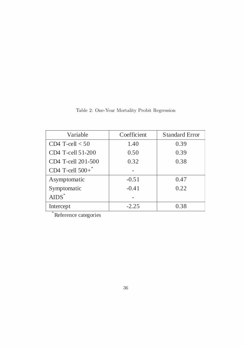
Table 2: One-Year Mortality Probit Regression
Variable Coefficient Standard Error
CD4 T-cell < 50 1.40 0.39
CD4 T-cell 51-200 0.50 0.39
CD4 T-cell 201-500 0.32 0.38
CD4 T-cell 500+* -
Asymptomatic -0.51 0.47
Symptomatic -0.41 0.22
AIDS* -
Intercept -2.25 0.38 * Reference categories
36

Table 3: Hypotheses
Prediction Test † Misperceived price Model Prediction 1: Negative correlation between health status and the decision to viaticate.
� � � �| Unhealthy, House | Healthy, Houset t�
� � � ��| Unhealthy, No House | Healthy, No Houset t�
Prediction 2a: Among healthy consumers, negative correlation between the decision to viaticate and the amount of nonliquid assets
� � � ��| Healthy, House | Healthy, No Houset t� ��
Prediction 2b: Among unhealthy consumers, a positive correlation between the decision to viaticate and the amount of nonliquid assets
� � � ��| Unhealthy, House | Unhealthy, No Houset t�
Prediction 3: Zero or negative correlation between liquid assets and the decision to viaticate
� � � �� �
| Income $2,000+ | Income $500 to $2,000
| Income below $500
t t
t
� �
�
�
�
Economic Model Prediction 1: Negative correlation between health status and the decision to viaticate.
� � � ���|Unhealthy, House | Healthy, Houset t�
� � � ��| Unhealthy, No House | Healthy, No Houset t� ��������
Prediction 2a: Among healthy consumers, positive correlation between the decision to viaticate and the amount of nonliquid assets
� � � ��| Healthy, House | Healthy, No Houset t� ��
Prediction 2b: Among unhealthy consumers, a positive correlation between the decision to viaticate and the amount of nonliquid assets
� � � �|Unhealthy, House |Unhealthy, No Houset t� ���
Prediction 3: Positive correlation between liquid assets and the decision to viaticate
� � � �� �
|Income $2,000+ | Income $500 to $2,000
> | Income below $500
t t
t
� �
�
�
† � �t� is the hazard of viaticating at time t.
� �
� �������
� �
� ��
37

Table 4: Empirical models of viatication hazards
Model 1 Model 2 Model 3 Model 4
Variables
Haz. Ratio (Conf Int.)
Haz. Ratio (Conf Int.)
Haz. Ratio (Conf Int.)
Haz. Ratio (Conf Int.)
Income Income < $500 1.00
(Ref Cat) 1.00
(Ref Cat) 1.00
(Ref Cat) 1.00
(Ref Cat) Income $500 –2000 1.08
(0.69 – 1.64) 0.90
(0.55 – 1.43) 1.05
(0.69 – 1.56) 0.88
(0.54 – 1.38) Income > $2000 1.42
(0.91 – 2.14) 1.02
(0.60 – 1.64) 1.35
(0.88 – 2.00) 0.98
(0.58 – 1.55)
House ownership and Health Status Healthy*House 1.00
(Ref Cat) 1.00
(Ref Cat) 1.00
(Ref Cat) 1.00
(Ref Cat) Unhealthy*House 3.90
(2.37 – 6.24) 4.35
(2.50 – 7.13) 2.71
(1.62 – 4.39) 2.93
(1.64 – 4.90) Unhealthy *NoHouse 2.16
(1.31 – 3.41) 2.46
(1.39 – 4.03) 2.25
(1.35 – 3.60) 2.60
(1.45 – 4.35) Healthy*NoHouse 1.55
(1.00 – 2.36) 1.83
(1.11 – 2.84) 1.31
(0.77 – 2.12) 1.56
(0.87 – 2.61) Bequest Motives Never Married - 1.00
(Ref Cat) - 1.00
(Ref Cat) Married - 1.12
(0.63 – 1.83) - 1.07
(0.62 – 1.70) Separated, Widowed, Divorced - 1.02
(0.71 – 1.42) - 1.09
(0.76 – 1.50) At Least One Child Alive - 0.73
(0.47 – 1.08) - 0.73
(0.48 – 1.07) Living Alone - 1.02
(0.75 – 1.37) - 1.01
(0.75 – 1.34) Demographics White - 1.00
(Ref Cat) - 1.00
(Ref Cat) Black# - 0.67
(0.44 – 0.98) - 0.73
(0.48 – 1.04) Hispanic# - 0.32
(0.13 – 0.62) - 0.33
(0.13 – 0.66) Other Race# - 0.55
(0.20 – 1.17) - 0.60
(0.21 – 1.25) Age - 1.21
(1.10 – 1.34) - 1.21
(1.10 – 1.33) Male - 1.03
(0.61 – 1.70) - 1.08
(0.65 – 1.77) Education Less Than High School - 1.00
(Ref Cat) - 1.00
(Ref Cat) High Schoolº - 0.65
(0.33 – 1.20) - 0.66
(0.34 – 1.21) Some Collegeº - 1.54
(0.84 – 2.66) - 1.64
(0.91 – 2.80) College º - 1.24
(0.61 – 2.31) - 1.30
(0.64 – 2.41)
38

Figure 1: Timeline for Two-Period Model
Per
iod 1
Sel
l life
insu
rance
F,
consu
me
C1,
and
bo
rro
w/l
end r
emai
nin
g a
sset
s
If d
ead:
beq
uea
th B
D
If a
live:
get
L2,
consu
me
C2,
and
beq
uea
th r
emai
nin
g a
sset
s B
S a
t th
e en
d
of
Per
iod
2
Nat
ure
rev
eals
whet
her
dea
d o
r al
ive
Per
iod 2
39

Figure 2: Budget Constraint for H3 Consumers
A
L
NL
C
W
F NL+F
Current Consumption
Bequests
BL+pF+NL1+r
40
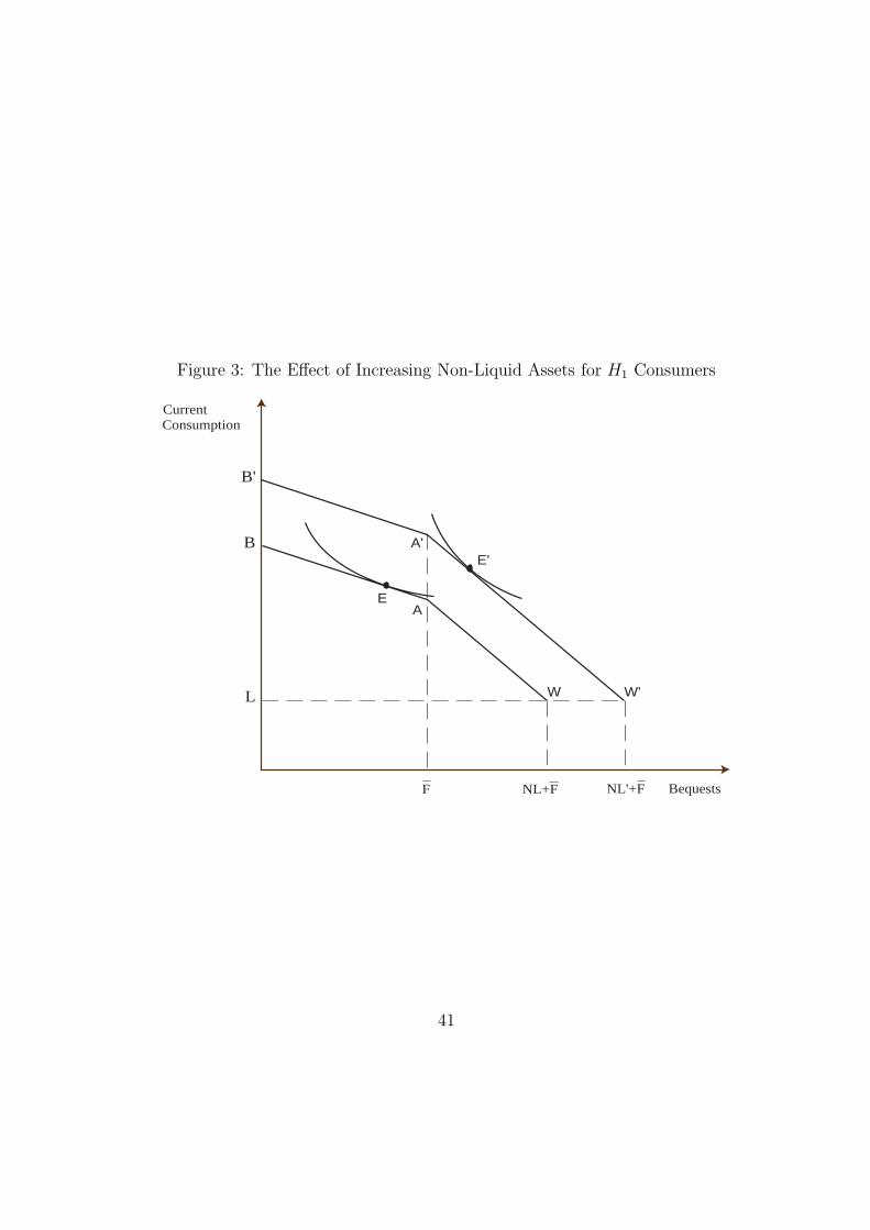
Figure 3: The Effect of Increasing Non-Liquid Assets for H1 Consumers
Bequests
B'
B
W W'
E
E'
A
A'
ConsumptionCurrent
NL'+F
L
NL+FF
41

Figure 4: The Effect of Increasing Non-Liquid Assets for H3 Consumers
Bequests
B'
B
NL+F
W W'
E'
C
C'
E G'
NL NL' NL'+F
ConsumptionCurrent
L
42

Figure 5: Proportion Not Viaticated by Health Status and House Ownership
years
0 1 2 3 4 5 6 7 8 9
0
.25
.5
.75
1
(Healthy, House) (Healthy, House)
(Healthy, NoHouse)
(Healthy, House)
(Healthy, NoHouse)
(Unhealthy, NoHouse)
(Healthy, House)
(Healthy, NoHouse)
(Unhealthy, NoHouse)
(Healthy, House)
(Healthy, NoHouse)
(Unhealthy, NoHouse)
(Unhealthy, House)
(Healthy, House)
(Healthy, NoHouse)
(Unhealthy, NoHouse)
(Unhealthy, House)
(Healthy, House)
(Healthy, NoHouse)
(Unhealthy, NoHouse)
(Unhealthy, House)
(Healthy, House)
(Healthy, NoHouse)
(Unhealthy, NoHouse)
(Unhealthy, House)
43