Market Formation in China from 1978

Rongsheng Tang∗

Shanghai University of Finance and Economics

July 2021

Abstract

This paper studies the formation of market economy in China from 1978

to 1992, a period in which market economy was introduced and developed

alongside planned government procurement for agricultural goods. Under

the “dual track system” (DTS), rural farmers were obligated to fulfill govern-

ment procurement before selling to the market, whereas urban consumers en-

joyed de facto subsidies to agricultural products. Using a neoclassical general

equilibrium model with heterogeneous firms and workers and input-output

linkage, this paper exploits historical data and analyzes allocation, prices,

and the formation of markets in China during this DTS period. Theoreti-

cally, while DTS will distort the resources allocation between rural and urban

(misallocation effect), it selects workers and farmers in the rural (selection ef-

fect). What is more, comparing to the economy under Soviet-style big bang

reform, DTS activates industrialization by providing intermediate goods with

lower-than-market price (activation effect). Quantitatively, directly switching

to market economy in 1978 would decrease total output by 4.5% as the activa-

tion effect dominates. On the intensive margin, reform on DTS ( procurement

price was getting closer to market price ) had contributed to total output by

4.4% from 1978 to 1992.

Keywords: Dual Track System; procurement; price distortion; misallocation

JEL Code: E65, N10, O43, O53

∗Institute for Advanced Research, Shanghai University of Finance and Economics; Key Lab-oratory of Mathematical Economics(SUFE), Ministry of Education, 777 Guoding Road, Shang-hai, China 200433 (e-mail: tang.rongsheng@sufe.edu.cn). I thank Chaoran Chen, Hanming Fang,Ernest Liu, Rody Manuelli, Yongseok Shin, Michale Song, Kjetil Storesletten, Ping Wang, YongqinWang, Yao Yao and Xiaodong Zhu for very helpful comments and suggestions. I have also bene-fited from comments by various seminar and conference participants. I am grateful for the finan-cial support from the National Natural Science Foundation of China (Grant No.71803112).

1 Introduction

This paper studies the formation of market economy in China from 1978 to 1992,a period in which market economy was introduced and developed alongsideplanned government procurement for agricultural goods. Unlike big bang reformin Soviet Union, DTS built a bridge between the planned and market systems inChina. How and how much did it activate Chinese economy at very beginning?How much has the price distortion affected different sectors? Using a neoclassi-cal general equilibrium model with heterogeneous firms and workers and input-output linkage, we exploit historical data and analyze allocation, prices, and theformation of markets in China during this DTS period. As it is believed that theagricultural reform in the 1980s mainly contributed to China’s growth, under-standing DTS will help understand the rise of the Chinese economy as well as theeffect of opening the internal market and gradual reform.

Under DTS, farmers were obligated to sell agricultural products to the govern-ment at a given price before selling the remaining products in the market. Urbanworkers and enterprises enjoyed quota benefits that allowed them to buy agri-cultural products at a lower price from the government.1 Before DTS, there wasno market, these products could only be sold to the government. As agriculturalproductivity was low, a minuscule quantity of agricultural products was left overafter procurement. Hence the whole economy was under the plan: firms pro-duced a certain quantity of products, and there was not much agricultural prod-uct surplus for the market. However, as agricultural productivity increased, theeconomy deviated from the plan. There was an increasing amount of agriculturalproducts, as well as a labor surplus in rural areas, and firms also expanded. Thisunplanned economic situation forced the government to relax market regulations,and to make a smooth transition, the government introduced DTS (one good withtwo prices) to partially open the market. Furthermore, to have sustainable growthand be afraid of market fluctuation, in the early stage of development, the gov-ernment implemented the policy to “help some people get rich first and then help theothers”. In the context of DTS, government subsidized urban firms and consumersvia quota benefit and taxed the rural people through the procurement. By the endof 1992, this policy was totally abolished, and all agricultural products were freeto be traded in.

1Although, in the real economy, the selling price from the government was usually higher thanthe purchasing price to cover transportation and other costs, we ignore these costs in the modelfor simplicity.

1

The internal market openness was an important policy, and the market struc-ture changed dramatically from the late 1970s. Historical data shows that theprice-adjusted market trade share of agricultural products increased from 5% in1975 to 45% in 1992. It is believed that the change was mainly due to the relaxationof the procurement requirement. In addition, the procurement price for compos-ite agricultural products has been increasing since 1978. In particular, the ratio ofmarket price to procurement price was 1.8 in 1978, dropped to 1.1 in 1989, and in1992 it was almost 1.2

We will focus on the impact of this procurement policy. First, it distorts theallocation of agricultural goods as urban firms enjoy the quota benefit, which inturn will affect the firm entries. Second, procurement placed burden on rural peo-ple, which will select them in farming and manufacturing production, shapingthe labor allocations. In order to consider them all, we build a neoclassical gen-eral equilibrium model with heterogeneous firms and workers and input-outputlinkage.

In the model, there are two separate labor markets: rural and urban. Rural hasfarmland and enterprises (Township and Village Enterprises, TVEs), while urbanonly has enterprises. There are two goods in the economy: agricultural goods andmanufacturing goods. Agricultural goods can only be produced on farmland; andmanufacturing goods can be produced in enterprises in both rural and urban. Inaddition, both goods can be used as consumption goods and intermediate goods.There is no migration between rural and urban,3 but rural people could chooseto be a farmer or a worker in rural enterprises. While farmers can plant on theland for free, workers don’t have this right. However, farmers have an obligationregarding procurement, but workers can waive it.

In addition, there are two types of ability: farming and manufacturing, whichcan be used only in agricultural goods and manufacturing goods production re-spectively. Enterprises are different in terms of productivity and the manufactur-ing of agricultural products. While urban enterprises enjoy the quota benefit withrespect to purchasing a certain amount of agricultural products below the marketprice, rural enterprises can only purchase the products at the market price.

Furthermore, although both enterprises and workers take the procurementand quota as given, essentially DTS was implemented to accelerate urban econ-omy first and then to help rural people get rich. More generally, the quantity on

2More details on DTS are documented in Section 2.3We ignore the migration because, in the data, the migration rate was only 0.19% in both 1978

and 1992. There is more discussion in Section 8.

2

procurement and quota reflect the magnitude the government values the urbanand rural. In the model, the procurement and quota quantity are determined bythe government to maximize the total weighted social welfare. As the weight onurban varies across years, the procurement level will change. Hence our analysiscould only focus on the procurement directly instead of the weights on rural orurban.

Theoretically, there are three main mechanisms on DTS: activation effect, se-lection effect, misallocation effect. While the first one is on the extensive margin,the latter two are effects on the intensive margin. Activation effect captures theeffect that, comparing with economy under Soviet-style big bang reform, as ur-ban enterprises enjoy the quota benefit, the gross manufacturing output could belarger, which in turn will increase the agricultural goods output as the interme-diate goods supply increases. This mechanism is especially effective when thereis migration barrier. First, due to the migration barrier, there is a labor produc-tivity gap between urban and rural, and the subsidy in intermediate goods willnarrow this gap and hence achieves the second best outcome. Second, when thereis surplus labor force in rural, marginal product of intermediate goods is high,then an increasing supply of intermediate goods will alleviate the negative im-pact of migration barrier under some circumstance. Selection effect representsthat procurement requirement will play a role as screening machine–only ruralpeople with relative high farming ability will stay as farmers. When the procure-ment price decreases, people who are less capable on farming in rural areas aremore likely to work in rural enterprises, which will increase the labor productivitythrough both decrease of labor force and increase of average farming ability, whilethe total output of agricultural products decreases which also shrinks its supplyas intermediate input. However, since the labor force in the rural enterprise getsmore, the net impact on rural enterprise output is ambiguous. Misallocation ef-fect means that some low productive firms in urban can survive due to quotabenefit, whereas firms with higher productivity in rural may not survive. As theintermediate input price for urban enterprise becomes lower, enterprises with lowproductivity enter the market and the total output increases, which increases agri-cultural goods production. The results are similar when the procurement quantitydecreases, except that urban output will decrease because of less quota benefit.Therefore, in the intensive margin effect, the impact of DTS is ambiguous.

For the quantitative analysis, we calibrate the model to the Chinese econ-omy each year from 1978 to 1992 and conduct several counterfactual experiments.Firstly, we take 1978 as benchmark and compare with the market economy, andwe also study the intensive margin effect as the the weight on urban changes.

3

Secondly, we take each year of 1979 − 1992 as benchmark and replace parame-ters with 1978’s value. Thirdly, we decompose the impact of different factors oneconomic growth and welfare. Finally, we study the economy with second-handmarket and frictionless economy as two extensions.

The quantitative results show that directly switching to market economy in1978 would decrease total output by 4.5% but increase rural welfare by 43.9% inequivalent consumption. That is to say, DTS has activated economy with sacrific-ing rural’s welfare. On the other hand, from 1978 to 1992, the procurement price isgetting closer to market price, which had contributed positively to total output by4.4% and rural welfare by 14.1%, and it contributed negatively to agricultural out-put by 18.1% and total welfare by 11.3%. The quantitative results also confirmedthat productivity improvement contributed mostly to Chinese economic growth.Furthermore, in the economy with second-hand market, there is not much changein output of different sectors, but the welfare changed significantly. For example,comparing to benchmark in 1978, the total output would decrease by 6%, the ruralwelfare would decrease by 36%. However, in frictionless economy, the impact ismuch larger. The total output in 1978 would be tripled comparing to benchmark,and the rural welfare would increase by more than 23 times.

Before delving into the details of the paper, we highlight one of contributions.In a recent debate between gradual and sudden transition, we take the stand thatthe gradual reform could activate the economy, pushing it out of low-equilibriumtrap. The main mechanisms are the following. First, due to the migration bar-rier, there is a labor productivity gap between urban and rural, and the subsidyin intermediate goods will narrow this gap and hence achieves the second bestoutcome. Second, given there is no migration allowed, the market economy is dis-torted. However, this distortion will be alleviated by subsidizing manufacturingproduction in urban, as industrialization requires agricultural goods as intermedi-ate inputs. And this effect will be amplified through input-output linkage in bothsectors. This mechanism is similar to the argument in Liu (2019) that given thereexists distortions, subsidizing upstream might alleviate the overall distortion, asthe upstream absorb more distortion through intermediate goods demanding, al-though in our setup, it is hard to tell which sector is upstream as they use inter-mediate goods from each other. We call this virtuous circle as “activation effect”or “extensive margin effect” in contrary to detrimental effect the distortion usu-ally cause, while we refer other two effects as “intensive margin effect”, including“misallocation effect” and “selection effect” as discussed above.

This study provides a framework to understand market formation, particu-larly when the market is partially open. The current Chinese economy is still un-

4

der transition to fully market economy. This dual track economy exists in differentscenarios. For example, there are different interest rates for State Owned Enter-prises (SOEs) and Private Owned Enterprises (POEs). While SOEs, taking advan-tage of low interest rate, can survive with lower productivity, POEs can borrowfrom SOEs, which is similar to the second-hand market discussed in the exten-sion. The current model is easy to extend to incorporate these scenarios and havepolicy implications. Moreover, the question studied in this paper can be related todiscussions about the role of industry policies and subsidies to infant industries,which is prevalent around the world especially in developing countries. The dualtrack system aims to protect urban enterprises as China went through the un-precedented episode. Therefore, a better understanding about the dual track sys-tem during this period would provide new empirical evidence about the impactof industry protection on the aggregate economy.

Related literature

We emphasize both the extensive and intensive margin effects of DTS in this pa-per. The analysis on extensive margin relates to studies on the economic transitionfrom planned economy to market economy, and the analysis on intensive margineffect relates to the studies on misallocation and selection in agricultural produc-tivity. We summarize them as follows.

On one hand, research on the Chinese economic transition from a planned toa market economy usually covers property rights and firm ownership ( Jin andQian (1998), Li (1997), Naughton (1994), Qian and Xu (1993)). Among them,Jin and Qian (1998) study the role of Township and Village Enterprises (TVEs),and Li (1997) studies the impact of economic reform on state-owned enterprises(SOEs). Different from these studies, our paper studies the procurement policyon goods markets. While Byrd (1991) analyzes the static and dynamic impactsof DTS on Chinese industry, Sicular (1988) builds a theoretical model to analyzeDTS in China’s agricultural sector. Our paper closely relate to Sicular (1988) as weboth study the procurement on agricultural goods. While she focuses on interac-tion of procurement and market price, we mainly study the impact on aggregateoutcome and allocative efficiency.

Some studies also analyze the effect of DTS on efficiency; however, there is nocommon agreement. While Lau et al. (2000) show that under some standard con-ditions, the dual track approach to market liberalization was a Pareto improve-ment, Young (2000) argues that the incremental reform would lead to the frag-

5

mentation of the domestic market and the distortion of regional production whenconsidering rent-seeking incumbents. Similar to McMillan et al. (1989) who pro-pose that the incentive will change under the market price, we also take the standon former one but emphasize that DTS will activate the economy through the vir-tuous circle of input-output linkage.

In addition, a section of the literature compares Chinese economy with East-ern European economies ( McMillan and Naughton (1992), Murphy et al. (1992),Sachs and Woo (1994), Li (1999), Roland and Verdier (2003)). Murphy et al. (1992)present a theory of partial economic reform and explain the reasons for the fail-ure of reforms in Russia in contrast to the successful Chinese reforms. Li (1999)also compares the Soviet-style big bang reform and the Chinese dual track reformand concludes that a transition policy is necessary to have a smooth transition.Guriev (2019) discusses several alternative explanations on the question of whySoviet Union did not follow China to reform the economy. Our study also relatesto Cheremukhin et al. (2017) who identify and study the impact of frictions onstructural transformation of Russia in 1885-1913 and 1928-1940 from an agrarianto an industrial economy.

On the other hand, our intensive margin analysis is related to research on mis-allocation and selection in agricultural productivity. The literature on misallo-cation covers the measurement, causes, and consequences (Hsieh and Klenow(2009), Buera et al. (2011),Song et al. (2011), Midrigan and Xu (2014), Restucciaand Rogerson (2017) among others). We contribute to the literature by interpret-ing DTS as a specific cause of misallocation, which distorts the market price ofagricultural goods. As we focus on DTS of agricultural goods, it also relates toliterature on agricultural productivity (Restuccia et al. (2008), Adamopoulos andRestuccia (2014), Chen (2017)). Adamopoulos et al. (2017) emphasizes the role ofselection across sectors, considering the constraint on productive farmers. Whilethey claim that productive farmers choose an occupation in a non-agricultural sec-tor, Lagakos and Waugh (2013) predict the opposite. Our model is in line with theformer because their model is calibrated with Chinese data.

As the agricultural and manufacturing goods production are connected throughinput-output linkage, our study also relates to Jones (2011) and Liu (2019) amongothers. In particular, Liu (2019) argues that, in a distorted economy, subsidizingthe upstream industries will generate positive network effects in China. We hada similar results that, given labor market distortion, price subsidy in agriculturalgoods had a positive effect on aggregate output.

6

Organization of the paper This paper is organized as follows: section 2 docu-ments the main facts, section 3 describes a quantitative model, section 4 illustratesthe main mechanisms, section 5 calibrates the model, section 6 presents the quan-titative results, section 7 presents the results under alternative parameters, section8 discusses issues on migration and capital, and section 9 concludes.

2 Facts

This section describes the main statistic characteristics of DTS. The data is mainlycollected from the National Bureau of Statistics (NBS) of China. The left panel ofFigure D.23 presents the ratio between procurement price and market price forcomposite materials from agricultural products. As shown in the figure, this ratiowas increasing from the middle of the 1970s. This means that the procurementprice was getting closer to the market price. The fact that all the values were lessthan 1 implies that the procurement price was lower than the market price.

NBS also provides information on the trade value in the market and under pro-curement. Market openness is calculated as the ratio of the value of agriculturalproducts traded in the market to the aggregate value of that from both the mar-ket and procurement. In addition, a price-adjusted ratio value is also calculatedby dividing price ratio on trade value from procurement.4 Right panel of FigureD.23 shows the trends of market share under both cases from 1953 to 1992. Start-ing from the middle 1970s, the market trade share increased from around 10% to45%, which confirms that the agricultural products market in China became moreopen.

One may think that the reduced difference between procurement price andmarket price may be due to the composition effect. As the economy grows, grainaccounts for a small portion of the agricultural output, whereas cash crops suchas cotton are more important. Furthermore, if the price between the two tracksis smaller for cash crops than it is for grains, then even if the price difference ofindividual crops does not change, the composition effect implies that the aggre-gated price difference is smaller. To address this issue, we compare the outputdata on grains and cash crops as shown in left panel of Figure D.24. It shows thatalthough, starting from 1978, the ratio of grain to the total of agricultural products

4The price-adjusted market share is calculated as : Vmarket

Vmarket+(Vall−Vmarket)

price ratio

, as price ratio is always

less than 1, this adjusted share is smaller than the un-adjusted share.

7

decreased, by 1992, this ratio was still higher than 75%. Therefore, the potentialcomposition effect cannot be substantial, and the fact that, in 1992, the procure-ment price was close to the market price is probably mainly due to the change ofpolicy on procurement.5

In addition, while agricultural productivity increased rapidly from 1978, thelabor market in China was segmented through the “Hukou” system. To absorbthe surplus rural labor force, more township and village enterprises (TVEs) wereestablished, particularly after 1984. Data on TVEs were collected from CSY orfrom the China TVEs Yearbook; however, there is some inconsistency betweenthese two sources. The value in the TVEs Yearbook is generally higher than thatin CSY. In our study, we use the data from CSY because it is more promising andpopular in the literature. The data have four components in the rural enterprisesbased on ownership: township, villages, private, and mixed. Because the dataon TVEs includes only the township enterprises before 1984, two versions of thestatistic characteristics are calculated. In the first version (v1), only township en-terprise data is used, and in the second version (v2), all the four components areincluded. As shown in Figure D.25, both the number of TVEs and its employmentshare in rural areas had increased. In 1984, there was a large increase in the num-ber of private TVEs, the output value share of which increased from 15% to 30%.Therefore, the jump in 1984 was mainly due to the addition of private TVEs in thedata.

The right panel of Figure D.24 presents the log value of the number of urbanenterprises from NBS. The number of urban enterprises increased from the early1970s. In what is similar to the case of TVEs, it also includes four components:SOEs and private, mixed, and others, including foreign enterprises. As only SOEdata are available for the period before 1984, two versions are presented. The firstversion includes only SOEs, and the second version includes all of them; the jumpin the figure is due to the inclusion of private enterprises after 1984.

In sum, the data shows that between 1978 and 1992, the market share of agri-cultural products increased a great deal; the ratio of procurement price to marketprice increased; the mass of TVEs and employment share in TVEs increased; andthe mass of urban enterprises increased.

5Due to lack of procurement price information on this two types of crops, we couldn’t havemore precise calculation.

8

3 A model on DTS

3.1 Environment

In the model, there are two separate labor markets: rural and urban. Rural hasfarmland and enterprises, but urban only has enterprises. There are two goods inthe economy: agricultural and manufacturing. While agricultural goods can onlybe produced on farmland, manufacturing goods can be produced in enterprisesin both rural and urban. In addition, both of them can be used for consumptionand intermediate input. Furthermore, there is no migration between rural and ur-ban, but rural people could choose to be a farmer or a worker in rural enterprises.While farmers can plant on the land for free, workers don’t have this right. How-ever, farmers have an obligation regarding procurement, but workers can waive it.On the other hand, urban people can only work in urban enterprises. Enterprisesare heterogeneous in productivity z, workers are heterogeneous in two-dimensionability h = (hF, hE) where hF is the ability of farming to yield agricultural productand hE is the ability to produce manufacturing goods.

The procurement and quota are modeled as follows. On the procurement side,for each unit of land, workers on farmland have an obligation to sell at least Qunits of agricultural products at price Pa to the government, and after fulfillingthis obligation, they are free to trade in the market. On the quota side, urban en-terprises are eligible to buy agricultural products at price Pa from the government;however, the total amount is limited by q. There is no second-hand market, thatis, firms are not allowed to sell agricultural goods brought from government asquota benefit in the market.

Furthermore, although both enterprises and workers take the procurementand quota as given, essentially DTS was implemented to accelerate urban econ-omy first and then to help rural people get rich. More generally, the quantity onprocurement and quota reflect the magnitude the government values the urbanand rural. In the model, the procurement and quota quantity are determined bythe government to maximize the total weighted social welfare. As the weight onurban varies across years, the procurement level will change. Hence our analysiscould only focus on the procurement directly instead of the weighted on rural orurban.

9

3.2 Agricultural goods production

Agricultural goods are produced on rural farmland, and land is equally distributedamong farmers. Denote Z the total amount of farmland and LRF the total numberof farmers, then the land size for each farmer is ZRF = Z

LRF.6 Given the intermedi-

ate goods xa and agricultural productivity Aa,the production function for a farmerh is

ya(h) = Aa(ZηRFhF

1−η)1−αa xαaa ,

where αa is the share of intermediate goods, 1− αa is the share of factor inputs,η is the land share of factor inputs. Given the ability distribution G(h) and thetotal labor force LR in rural area, aggregate production of agricultural goods is theaggregation of output from workers on farmland denoted as RF

Ya = LR

∫RF

ya(h)dG(h). (1)

Given the procurement requirement Q for each piece of land, farmers choose in-termediate input xa and quantity selling to government Qa to maximize the netvalue of agricultural goods production

maxxa>0,Qa≥QZRF

Pa Aa(ZηRFhF

1−η)1−αa xαaa − Pmxa − (Pa − Pa)Qa. (2)

3.3 Manufacturing goods production

Manufacturing goods could be produced in rural (R) and urban (U) areas. Insector j = R, U, denote Aj is the location specific productivity, Hj is the humancapital level, xj is the input of agricultural goods, the production function for afirm z is

yj(z) = Ajzγj(H1−αjj x

αjj )

1−γj , j = R, U

where 1− γj is the span of control and αj, 1− αj denote the share of agriculturalgoods and human capital respectively. The assumption that both agriculturalgoods and manufacturing goods are used as intermediate goods follows Jones(2011) but differs from Restuccia et al. (2008) where only manufacturing goods are

6In the real economy, land is equally distributed across households weighted by member num-ber; however, for split households or moved workers, the policy is not clear at the national level.Some may still have land, while others may not. To avoid this confusion, we assume that the landis distributed only among people who are still working on farmland.

10

used as intermediate goods. This is based on the fact that, in the context of China,the Input-Output table shows the share of agricultural goods used in producingnon-agricultural goods is significant.7

Following Brandt et al. (2018), we assume productivity z follows Pareto distri-bution F(z), and there are potential mass Mj enterprises. The total output is theaggregation over active firms denoted by Dj, in particular,

Yj = Mj

∫Dj

yj(z)dF(z), j = R, U. (3)

As there is no labor mobility across rural and urban areas, the wage rate will bedifferent, denoted by wR and wU. Given entry cost CR, the profit for firm z in ruralis

πR(z) = maxHR,xR

PmyR(z)− wRHR − PaxR − CR. (4)

The profit for firm z in urban is

πU(z) =

maxHU ,xU

PmyU(z)− wU HU − PaxU − CU if xU ≤ q

maxHU ,xU

PmyU(z)− wU HU − PaxU + (Pa − Pa)q− CU if xU > q.(5)

In the case of xU > q, the profit function can be written as

πU(z) = PmyU(z)− wU HU − (1− Pa − Pa

Pa

qxU

)PaxU − CU.

As 0 < Pa−PaPa

qxU

< 1, the quota benefit and the procurement price imply a lower-

than-market input price in general, and Pa−PaPa

qxU

is an implicit distortion on inter-mediate goods allocation due to quota benefit. Hence, in this model, the distor-tion is caused by quota benefit. As the amount of input xU increases, the ex-postprice (1− Pa−Pa

Pa

qxU)Pa gets closer to the market price Pa; and the price distortion

decreases as xU increases.

7Data of Input-Output table from 1981 to 1992 shows that while the share of non-agriculturalgoods used in producing agricultural goods is 0.157, the share of agricultural goods used in pro-ducing non-agricultural goods is 0.066. It is a bit lower because the price of agricultural goods isgenerally much lower; however, it is persistent and high in some industries (e.g., the food industry,the textile industry, etc.). More details are documented in Table D.1 and Table D.2.

11

3.4 Workers

A worker’s utility depends on consumption of agricultural goods (a) and manu-facturing goods (m)

u(a, m) = θlog(a− a) + (1− θ)log(m),

subject to budget constraint Paa + Pmm ≤ I, where θ is the weight on agriculturalgoods; a is the subsistence level of agricultural goods; Pa, Pm are the market pricesof agricultural and manufacturing goods, respectively, and I is worker’s income.Then the indirect utility function is

V(I) = [θlog(θ

Pa) + (1− θ)log(

1− θ

Pm)] + log(I − Pa a).

Rural workers could choose working in rural enterprises (RE) or on the farmland(RF). The income in RE is from the wage and share of profit from rural enterprises,that is,

IRE(h) = wRhE +ΠR

LR(6)

where ΠR = MR∫

DRπR(z)dF(z) is the total profit from rural enterprises, and

people in rural share the profit equally. On the other hand, the net income forfarmer with ability h is given by

IRF(h) = (1− αa)Paya(h)− (Pa − Pa)Qa +ΠR

LR(7)

It can be rewritten as IRF(h) = [(1− αa)− Pa−PaPa

Qaya(h)

]Paya(h) + ΠRLR

, then Pa−PaPa

Qaya(h)

is the price distortion faced by farmers which is caused by procurement. In partic-ular, as Qa < ya(h) and Pa < Pa, this distortion is increasing in procurement levelQa.

Workers in urban areas will only work in urban enterprises UE whose incomecome from urban wage and profit share. The total profit from urban enterprises isΠU = MU

∫DU

πU(z)dF(z), which is equally distributed among the urban people,

then the income for urban household is IU(h) = wUhE + ΠULU

.

12

3.5 Government

In the above setting, both enterprises and workers take the procurement (Q) andquota (q) as given. Essentially DTS was implemented to accelerate urban econ-omy first and then to help rural people. More generally, the quantity on procure-ment and quota reflect the magnitude the government values the urban and rural.Hence, in the model, the procurement and quota quantity are determined by thegovernment to maximize the total weighted social welfare.

As a direct effect, high procurement will hurt farmers’ welfare but make ur-ban people better off. However, as manufacturing goods output increases, the in-termediate goods in agricultural production will be cheaper, which will improvefarmer’s welfare. The total welfare in urban is the aggregate of all the urban work-ers, LU

∫U V(IU(h))dG(h), and the welfare in rural is sum of enterprises work-

ers and farmers, LR[∫

RE V(IRE(h))dG(h) +∫

RF V(IRF(h))dG(h)]. Denote χU theweight on welfare for urban household, the government’s problem is to set theprocurement and quota level to maximize the total welfare, that is,

maxq,Q≥0

χU LU

∫DU

V(IU(h))dG(h) + (1− χU)LR[∫

RFV(IRF(h))dG(h) +

∫RE

V(IRE(h))dG(h)] (8)

s.t.MU

∫DU

min{xU(z), q}dF(z) = QZ (9)

where the budget constraint says the government will sell all the agriculturalgoods brought from farmers to urban firms as the quota benefit. Therefore, inthis model, procurement and quota are endogenously determined, as the weighton urban varies across year, the procurement level will change, and the impact oneconomy will be different.

3.6 Equilibrium

In order to characterize the equilibrium, we define the following aggregate vari-ables. The total demand for manufacturing goods as intermediate input is

xa = LR

∫RF

xa(h)dG(h) (10)

The total demand for agricultural goods as intermediate input is

xj = Mj

∫Dj

xj(z)dF(z), j = R, U (11)

13

The total demand for agricultural goods for consumption in rural area is

aR = LR

∫RE

aRE(h)dG(h) + LR

∫RF

aRF(h)dG(h) (12)

The total demand for agricultural goods for consumption in urban area is

aU = LU

∫UE

aU(h)dG(h) (13)

The total demand for manufacturing goods for consumption in rural area is

mR = LR

∫RE

mRE(h)dG(h) + LR

∫RF

mRF(h)dG(h) (14)

The total demand for manufacturing goods for consumption in urban area is

mU = LU

∫UE

mU(h)dG(h) (15)

The total human capital demand in sector j = R, U is

HDj = Mj

∫Dj

Hj(z)dF(z), j = R, U (16)

The total human capital supply in rural area is

HSR = LR

∫RE

hEdG(h) (17)

The total human capital supply in urban area is

HSU = LU

∫UE

hEdG(h). (18)

Equilibrium The equilibrium is characterized by agricultural goods selling togovernment {Qa} and intermediate goods {xa(h)}, labor allocation in rural {LRF, LRE},enterprises factor input {Hj(z), xj(z)}, j = R, U , and procurement and quota level{Q, q}, wage rate {wR, wU}, and goods prices {Pa, Pm} such that

1. {Qa, xa(h)}maximizes rural worker income as in equation (2).

2. {LRF, LRE} is the result of the occupation choice for rural people, as in equa-tion (7) and (6).

3. {Hj(z), xj(z)}, j = R, U maximizes enterprise profit in equation (4) and (5).

14

4. {Q, q} solves government’s problem to maximize total welfare as in equa-tion (8) and (9).

5. wR, wU, Pa, Pm clear labor markets and goods markets.

(a) Rural labor market clear, HDR = HS

R, as in equation (16) and (17).

(b) Urban labor market clear, HDU = HS

U as in equation (16) and (18).

(c) Agricultural goods market clear, Ya = xR + xU + aR + aU as in equation(1), (11), (12), and (13).

(d) Manufacturing goods market clear, YR + YU = xa + mR + mU as inequation (3), (10), (14), and (15).

4 Theoretical results

In this section, we illustrate three main mechanisms of DTS: activation effect, se-lection effect, misallocation effect. Activation effect captures the idea that as ur-ban enterprises enjoy the quota benefit, the gross manufacturing output couldbe larger, which will increase the agricultural goods output as the intermediategoods supply increases. Selection effect represents that procurement requirementwill play a role as screening machine–only rural people with relative high farmingability will stay as farmers. Misallocation effect means that some low productivefirms in urban can survive due to quota benefit, whereas firms with higher pro-ductivity in rural may not survive. To illustrate these mechanisms, we simplifythe benchmark model and only focus on one channel in each subsection in below.

4.1 Activation effect

To illustrate the activation effect, we simplify the model in the following way. Bothworker’s ability and firm’s productivity are homogeneous, agricultural goods areproduced in rural, enterprises are located only in urban, and there is no migra-tion. Procurement is determined by the government to maximize the total wel-fare. Otherwise it largely follow the quantitative model as presented in AppendixA.1.

We compare the general equilibrium results in market economy with that inthe DTS in the case of xU ≤ q. Given procurement requirement Q, denote Pa

Pa= κP,

15

and normalize Pm = 1, market clear condition under DTS requires

[1− θ(1− αa)]Aa[αaPa Aa]αa

1−αa Zη L1−ηR + θ(1− κP)QZ− [(1− θ)a]LR

=(1− θ)aLU − θCUPa

+ (κPPa

αa(1− γU)AU)

1αU (1−γU )−1 L

(αU−1)(1−γU )αU (1−γU )−1

U {1 + θκp[βUαU

+γU

αa(1− γU)]} (19)

such that ( κPPaαa(1−γU)AU

)1

αU (1−γU )−1 L(αU−1)(1−γU )

αU (1−γU )−1U ≤ QZ. On the other hand, the equi-

librium condition in market economy implies

[1− θ(1− αa)]Aa[αaPa Aa]αa

1−αa Zη L1−ηR − [(1− θ)a]LR

=(1− θ)aLU − θCUPa

+ (Pa

αa(1− γU)AU)

1αU (1−γU )−1 L

(αU−1)(1−γU )αU (1−γU )−1

U {1 + θ[βUαU

+γU

αa(1− γU)]} (20)

0PP

a

DP

a

MP

a

D 0.4

Pa

0

0.1

0.2

0.3

0.4

0.5

0.6

0.7

0.8

0.9

1

Pa

SS-DTS

DD-DTS

SS-MKT

DD-MKT

0 Pa

MP

a

D 0.4

Ya

0

Ya

M

Ya

D

Ya

Ya(P

a)

0 Pa

MP

a

D 0.4

YU

0

YU

MY

U

D

YU

YU

D(P

a)

YU

M(P

a)

Figure 1: Activation effectNote: This figure compares the equilibrium in homogeneous model under DTS and market econ-omy. Left panel illustrates the equilibrium prices, SS-DTS and SS-MKT is the agricultural goodssupply in urban (Ya − xR) under DTS and market economy respectively; DD-DTS and DD-MKT isthe agricultural goods demand in urban (aU + xU) under DTS and market economy respectively.Right and middle panel illustrate the equilibrium outputs. The middle panel is agricultural goodsgross output, and the function forms are the same under DTS and market economy. The rightpanel is manufacturing goods gross output under DTS (YD

U (Pa)) and market economy (YMU (Pa)).

Figure 1 compares the equilibrium price and outputs under DTS (PDa ) and mar-

ket economy (PMa ), which is also summarized in Proposition 1. It shows that if κP

and Aa are small enough, under DTS the outputs in both agricultural and manu-facturing sector are higher. That is to say, DTS activates the economy when agri-cultural productivity is low enough. Note we take κp as exogenous, and Pa isgeneral equilibrium price, by this setting, procurement price is also general equi-librium result but subject to the price distortion.

16

Proposition 1. In the homogeneous model, 1) there always exists PMa > κPPD

a ; 2) themanufacturing goods gross output under DTS is always higher than market economy; 3)when κP and Aa are small enough, the agricultural goods gross output under DTS is alsohigher than that in market economy.

Proof: see Appendix A.1.6.

4.1.1 Role of lacking migration

To better illustrate activation effect, we highlight the role of lacking migration.First, due to the migration barrier, there is a labor productivity gap between ur-ban and rural, and the subsidy in intermediate goods will narrow this gap andhence achieves the second best outcome. Second, given the labor mobility is for-bidden, there are surplus labor force in rural, that is, the marginal product ofintermediate goods is very high, then subsidizing urban might increase interme-diate goods supply in rural which in turn will increase agricultural goods produc-tion. Technically, suppose there is subsidy dXu to urban as intermediate goods, itwill increase manufacturing output and also the product sold to rural as inter-mediate goods, denoting it as a function of subsidy f (dXu), then as long as themarginal product of intermediate goods in rural (MPX) is high enough so thatMPX · f (dXu) > dXu, then the gross agricultural output will be higher. Thismechanism is similar to the argument in Liu (2019) that, given there exists distor-tions, subsidizing upstream might alleviate the overall distortion, as the upstreamabsorb more distortion through intermediate goods demanding, although in oursetup, it is hard to tell which sector is upstream as they use intermediate goodsfrom each other.

We then compare the economy with and without migration graphically, show-ing that the results might change if there is no migration barrier. Figure 2 presentsthe comparison between market economy and DTS with migration under case ofxU ≤ q where the parameters are the same as those used in Figure 1. Comparingit with the results without migration in Figure 1 shows that, with migration, man-ufacturing goods production in urban would be higher under market than DTSand the agricultural goods production is still higher under DTS. Moreover, in thiscase, we have xM

U < xDU and xM

a > xDa .8 The interpretation is that in the market

economy urban firm will purchase less intermediate goods (xMU < xD

U), however,as there is more labor force, the output is higher (yM

U > yDU). On the other hand, as

more people migrate to urban, it is more profitable for farmers to buy more inter-mediate goods (xM

a > xDa ), but the output is still lower under market economy as

8This result is not shown in the Figure, but it can be computed in Appendix A.2.

17

the labor force effect dominates.

0PP

a

DP

a

DP

a

M 0.4

Pa

0

0.1

0.2

0.3

0.4

0.5

0.6

0.7

0.8

0.9

1

Pa

SS-DTS

DD-DTS

SS-MKT

DD-MKT

0 Pa

DP

a

M 0.4

Ya

0

Ya

M

Ya

D

Ya

Ya

D(P

a)

Ya

M(P

a)

0 Pa

DP

a

M 0.4

YU

0

YU

D

YU

M

YU

YU

D(P

a)

YU

M(P

a)

Figure 2: Activation effect with migrationNote: This figure compares the equilibrium under DTS and market economy in homogeneousmodel with migration. The parameters are the same as those used in Figure 1. Left panel illustratesthe equilibrium prices, SS-DTS and SS-MKT is the agricultural goods supply in urban (Ya − xR)under DTS and market economy respectively; DD-DTS and DD-MKT is the agricultural goodsdemand in urban (aU + xU) under DTS and market economy respectively. Right and middle panelillustrate the equilibrium outputs. The middle panel is agricultural goods gross output under DTS(YD

a (Pa)) and market economy (YMa (Pa)). The right panel is manufacturing goods gross output

under DTS (YDU (Pa)) and market economy (YM

U (Pa)).

4.2 Selection effect

To illustrate the selection effect, we study the occupational choice in rural, assum-ing enterprises are only located in urban and migration between rural and urbanis allowed. Given Pa > Pa, the constraint is always binding, that is, Qa = QZRF.Then there is a cutoff of ability profile regarding occupational choice in rural area

hE = L(hF) =1

wU{(1− αa)Pa(

αaPa

Pm)

αa1−αa [Aa(Zη

RFhF1−η)βa ]

11−αa − (Pa − Pa)QZRF},

and the ability profile of workers in enterprises is UE = {h : hE > L(hF)}, and forfarmers, it is RF = {h : hE < L(hF)}. Then, the direct effect of high procurementis that, as Q increases or Pa decreases, people who are less capable on farming inrural areas are more likely to work in enterprises as shown in Figure 3, which willincrease the labor productivity through both decrease of labor force and increaseof average ability, while the total output of agricultural products decreases.

However, there is an indirect or feedback effect. Since ZRF = ZLRF

, the average

18

land size ZRF is getting larger, then it will discourage the migration. Hence themagnitude of effect is unclear even in partial equilibrium, and it will be furtherexamined in section 6.

0.1 0.2 0.3 0.4 0.5 0.6 0.7 0.8 0.9 1

hF

0

0.1

0.2

0.3

0.4

0.5

0.6

0.7

0.8

0.9

1

hE

occupational choice

Qbar=0.9

Qbar=1.1

Figure 3: Selection effectNote: This figure illustrates the response of occupational choice as procurement level changes,with abilities below the line people will choose to work on farmland, while for those of abilitiesabove the line will choose to work in enterprises.

4.3 Misallocation effect

To illustrate the misallocation effect, we focus on urban enterprise’s behavior as-suming enterprises are only located in urban and migration between rural andurban is not allowed. As shown in Appendix A.4, given a fixed entry cost CU,there exists productivity cutoff z∗U, zL, zH such that the intermediate goods de-mand function and profit function are

xU(z) =

0 z ≤ z∗UxL(z) z∗U < z ≤ zL

q zL < z ≤ zH

xH(z) z > zH

, and πU(z) =

0 z ≤ z∗UπL(z) z∗U < z ≤ zL

πM(z) zL < z ≤ zH

πH(z) z > zH

.

This mechanism is similar to Guner et al. (2008). The interpretation is thatthe unproductive firm (z ≤ z∗U) will not enter the market. Low productive firm

19

(z∗U < z ≤ zL) will have intermediate input under the quota benefit (xL(z) < q).9

There is a positive mass of firm that will have intermediate input q. If the firmwants to buy agricultural goods above the quota level, the marginal cost (price) ofagricultural goods will jump from Pa to Pa; hence, firms with productivity slightlyhigher than zL may not be able to cover this cost and stick to the quota level. Thenthe very productive firm will have a higher intermediate input (xH(z) > q).

0 z*z

*

cz

Lz

H0.8

z

0

CU

0.4

profit

counter-factual

0 z*z

*

cz

Lz

H0.8

z

0

q_bar

0.2x

demand function

counter-factual

Figure 4: Misallocation effectNote: This figure illustrates the firm’s decision. The solid line represents the profit function in leftpanel and intermediate goods demand function in the right panel, while the dash line representthe result of removing the quota benefit and the intermediate goods is under the market price.

Figure 4 illustrates the demand and profit function. The left panel shows thatless firm will enter the market if there is no procurement (z∗ < z∗c ), and the rightpanel shows that firm will invest less in intermediate goods if there is no pro-curement as the dash line is below the solid line in the figure. The followingproposition summarizes results of comparative statics in partial equilibrium.

Proposition 2. With DTS, the entry level productivity z∗U is increasing in CU, Pa, wU

and decreasing in AU, and the cutoff zL is increasing in Pa, q, wU and decreasing in AU.In addition, the welfare for rural (urban) people is decreasing (increasing) in procurement.

Proof: Lemma 4- Lemma 7 in Section A.4 will prove this proposition.

9The existence of xL(z) < q is due to no second-hand market, otherwise firms can sell quotabenefit under the market price and hence they will buy intermediate goods at least at quota levelregardless productivity. We will further quantify the impact with second-hand market in section6.4.

20

5 Calibration

As in Brandt et al. (2018), firm productivity z follows Pareto distribution withminimal productivity zR,min = zU,min = 1, that is, F(z) = 1 − (1

z )θj , z > 1, j =

U, R, with θR = θU = 1.05, and we also set γR = γU = 0.15. In addition, asin Adamopoulos et al. (2017), the abilities jointly follow log normal distribution

G(hF, hE) ∼ LN(µ, Σ) where µ = (µF, µE) and Σ =

(σ2

F σFE

σFE σ2E

). The parameters

are µF = 0.16, µE = 0.88, σF = 1.48, σE = 0.95, and ρFE = −0.35, that is tosay, ability hF and hE are negatively correlated. On the contrary, Lagakos andWaugh (2013) use US data and assume the abilities following Fréchet distribution

G1(hF) = e−h−θFF , G2(hE) = e−h−θE

E and the parameters are θF = 5.3, θE = 2.7,ρ = 3.5.10 As the result in Adamopoulos et al. (2017) is based on Chinese data, weassume that it also follows joint log normal distribution in our study.

The potential mass of enterprises MR, MU are assumed to proportional to la-bor force in rural enterprises and urban enterprises respectively, without losinggenerality, we assume that MR = LRE, MU = LU. In addition, LR, LU are fromemployment ratio in rural and urban, respectively; Pa

Pais the procurement to mar-

ket price ratio; from the Input-Output table, the share of intermediate goods innon-agricultural goods in agricultural production is αa = 0.157, which is lowerthan 0.4 in the US as in Restuccia et al. (2008). The share of agricultural goodsused as intermediate goods is αR(1− γR) = 0.066, which is much lower than theaverage share of the intermediate goods 0.68 in Jones (2011). This share givesαR = 0.078 as in Adamopoulos et al. (2017); the land share to labor share ratio is

η1−η = 0.36

0.46 , which implies η = 0.439. Then the land share is (1− αa)η = 0.370and labor share is αaη = 0.473, which are close to those in Adamopoulos et al.(2017). We set θ = 0.005 as in literature (e.g. Chen (2017) ). Table 1 summarizesthe results.

We calibrate the rest of parameters in two steps. First, we target the averagevalue between 1978 and 1992 in the data. Urban productivity AU is normalized as1. Agricultural productivity Aa is calibrated to match the output ratio between ru-

10 In Lagakos and Waugh (2013), joint distribution takes the following function form:

G(hF, hE) = Cp[G1(hF), G2(hE)], hF > 0, hE > 0,

where

Cp(u, v) = −1ρ

log[1 +(e−ρu − 1)(e−ρv − 1)

e−ρ − 1].

21

ral enterprise and agriculture YR/Ya where YR is the real value of output in TVE,Ya is the total real value of agricultural output selling in market and under pro-curement. Rural productivity AR is calibrated to match the output ratio betweenurban and rural enterprises YU/YR where YU is the real value of output in urban.The entry costs are calibrated as in Brandt et al. (2018) that assuming that the hu-man capital of a margin firm is 1, that is, HR(z∗R) = 1,and HU(z∗U) = 1, hencethe entry cost can be written as Cj =

γjwj(1−αj)(1−γj)

, j = R, U. The welfare weightχU is calibrated to match market share (ms) which is defined as the proportionof agricultural goods value selling in market to the total value. Subsistence levela is calibrated to match the employment share in rural enterprises LRE/LR; andtotal land size Z is calibrated to match the average earning ratio between urbanand rural EU/ER, where EU, ER are the average household disposable income inurban and rural respectively.

Table 2 lists the parameters in this step. Generally the model matches the av-erage value well except for it overestimates the employment ratio in rural enter-prises. Note that χU = 0.9178 implies the government value urban much higherthan rural. This is consistent with the real economy that, at the beginning of re-form the urban is favored by the policy.11 In addition, CR < CU implies the entrycost in rural is much lower than that in urban. It is consistent with facts in FigureD.25 that, in the early stage, there is a large number of TVEs entering the market.

Second, we assume total land size Z is constant across year and calibrate otherparameters year by year. In particular, CR, CU, MR, MU and a, χU are calibratedin the same way as the first step. The productivities Aa, AR, AU are calibrated tomatch the real outputs Ya, YR, YU year by year by normalizing the average val-ues to be 1. Table 3 summarizes the parameters. In the calibration, we simulatethe model and minimize the error between the simulated moment and the datamoment as in Lagakos and Waugh (2013), and the detail of this algorithm is inAppendix B.

Figure 5 presents the model and data for targeted moments in each year wherethe dash line represents the data and the solid line represents the model for tar-geted variables where the output Ya, YR, YU are normalized as 1 in average forboth the data and the model. It shows the model matches data well. Moreover,Figure 6 shows it also match the following untargeted moments well: agriculturalgoods price (Pa), average earning in rural and urban (ER, EU), procurement level(Q). The dash line is data and the solid line is model. All the variables are nor-

11This is said in the early stage of development that “help some people get rich first and thenhelp the others”.

22

malized as 1 in average value for both the data and the model. Finally, Figure7 presents the parameters across years, including agricultural productivity (Aa),rural productivity (AR), urban productivity (AU), weight on urban in social wel-fare (χU), number of potential entrant in urban and rural (MU, MR), entry costs inurban and rural (CU, CR). It shows that there is a clear trend of all the parameterswhich is important for counterfactual analysis.

Table 1: Parameters without solving model

parameters value target or sourceαj αR = αU = 0.078,αa = 0.157 Input-Output tableη 0.439 Adamopoulos et al. (2017)

γR, γU 0.15 Brandt et al. (2018)µF, µE, σF, ρFE, σE µF = 0.16, µE = 0.88, σF = 1.48, ρFE = −0.35, σE = 0.95 Adamopoulos et al. (2017)

θR, θU 1.05 Brandt et al. (2018)θ 0.005 Chen (2017)

Note: This table lists the parameters calibrated without solving the model. αj, j = a, R, U,η, γR, γU are the share in production function calculated from the Input-Output table andthe literature (Adamopoulos et al. (2017), Brandt et al. (2018)), µF, µE, σF, ρFE, σE are theparameters of productivity distribution adopted from Adamopoulos et al. (2017), θR, θUare the parameters of ability distribution from Brandt et al. (2018), θ is the preferenceparameter (Chen (2017)).

Table 2: Parameters in average

parameters description value target model dataAa agricultural productivity 0.0418 YR/Ya 1.2243 1.4653AR TVE productivity 0.2184 YU/YR 3.9809 4.1039χU welfare weight 0.9178 ms 0.3139 0.2674a subsistence level 0.0106 LRE/LR 0.3595 0.1651

CR entry cost in rural 0.0166 HR(z∗R) = 1CU entry cost in urban 0.1041 HU(z∗U) = 1MR potential entrant 0.1226 LRE 0.1226 0.1226MU potential entrant 0.2550 LU 0.2550 0.2550Z total land size 3.1810 EU/ER 2.9317 2.2174

Note: This table lists the parameters calibrating targets in average value from 1978 to1992. Aa, AR are productivities, χU is welfare weight on urban household, a is subsis-tence level in utility function, CR, CU are the entry cost in rural and urban, MR, MU arethe potential entrant in rural and urban, Z is the total land size.

23

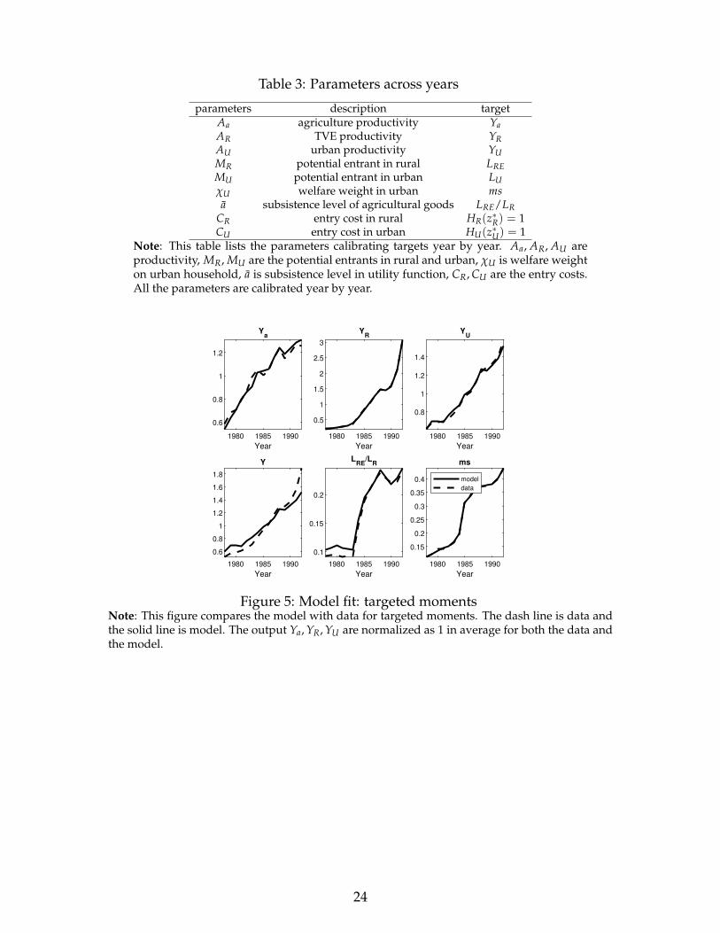
Table 3: Parameters across years

parameters description targetAa agriculture productivity YaAR TVE productivity YRAU urban productivity YUMR potential entrant in rural LREMU potential entrant in urban LUχU welfare weight in urban msa subsistence level of agricultural goods LRE/LR

CR entry cost in rural HR(z∗R) = 1CU entry cost in urban HU(z∗U) = 1

Note: This table lists the parameters calibrating targets year by year. Aa, AR, AU areproductivity, MR, MU are the potential entrants in rural and urban, χU is welfare weighton urban household, a is subsistence level in utility function, CR, CU are the entry costs.All the parameters are calibrated year by year.

1980 1985 1990

Year

0.6

0.8

1

1.2

Ya

1980 1985 1990

Year

0.5

1

1.5

2

2.5

3

YR

1980 1985 1990

Year

0.8

1

1.2

1.4

YU

1980 1985 1990

Year

0.6

0.8

1

1.2

1.4

1.6

1.8

Y

1980 1985 1990

Year

0.1

0.15

0.2

LRE

/LR

1980 1985 1990

Year

0.15

0.2

0.25

0.3

0.35

0.4

ms

model

data

Figure 5: Model fit: targeted momentsNote: This figure compares the model with data for targeted moments. The dash line is data andthe solid line is model. The output Ya, YR, YU are normalized as 1 in average for both the data andthe model.

24

1980 1985 1990

Year

0.5

1

1.5

2

Pa

1980 1985 1990

Year

0.5

1

1.5

ER

1980 1985 1990

Year

0.5

1

1.5

2

EU

1980 1985 1990

Year

0.5

1

1.5

Q_\bar

model

data

Figure 6: Model fit: untargeted momentsNote: This figure compares the model with data for untargeted moments: agricultural goods price(Pa), average earning in rural and urban (ER, EU), procurement level (Q). The dash line is data andthe solid line is model. All the variables are normalized as 1 in average value for both the data andthe model.

1975 1980 1985 1990 1995

Year

0

0.1

0.2

Aa

1975 1980 1985 1990 1995

Year

0

0.05

0.1

AR

1975 1980 1985 1990 1995

Year

2

4

6

AU

1975 1980 1985 1990 1995

Year

0.97

0.98

0.99U

1975 1980 1985 1990 1995

Year

0.24

0.25

0.26

MU

1975 1980 1985 1990 1995

Year

0.74

0.75

0.76

MR

1975 1980 1985 1990 1995

Year

0.5

1

CU

1975 1980 1985 1990 1995

Year

0

1

2

CR

Figure 7: ParametersNote: This figure presents parameters across years: agricultural productivity (Aa), rural produc-tivity (AR), urban productivity (AU), weight on urban in social welfare (χU), number of potentialentrant in urban and rural (MU , MR), entry costs in urban and rural (CU , CR).

25

6 Quantitative analysis

With the parameters calibrated, we quantitatively analyze the impact of DTS inseveral experiments. Firstly, we take 1978 as benchmark and do counterfactualanalysis on different factors, and we also study the scenario when switching tomarket economy in 1978. Secondly, we take each year of 1979-1992 as bench-mark and study the effect when parameters are set with 1978’s values. Thirdly,we decompose the impact of different channels on economic growth and welfare.Fourthly, we study the economy with second-hand market and frictionless econ-omy as two extensions.

6.1 Counterfactual analysis

To understand the mechanism and importance of each factor, we take 1978 asbenchmark and set parameters with 1992’s value. In Table 4, the column of “bench-mark” is the results in 1978, and each column under “counterfactual case” liststhe results when setting this parameter in 1992’s value while keeping others thesame as in 1978; and in the column of “market”, we set Pa

Pa= 1 and Q = 0, that

is, the government doesn’t set procurement requirement. The results show that

Table 4: Counterfactual analysis in 1978

variable benchmark counterfactual result (value)Aa AR AU Pa/Pa χU market

Ya 0.073 0.227 0.085 0.087 0.073 0.072 0.071YR 0.01 0.004 0.166 0.004 0.002 0.003 0.002YU 2.264 2.374 2.228 4.788 2.126 2.211 2.159LRF/LR 0.743 0.793 0.392 0.704 0.955 0.898 0.971ms 0.112 0.464 0.809 0.188 0.156 0.529 1Y 2.408 2.528 2.51 5.084 2.251 2.415 2.299xa 0.04 0.038 0.024 0.085 0.023 0.05 0.026M∗R 0.306 0.147 0.763 0.151 0.082 0.093 0.069M∗U 0.116 0.128 0.129 0.237 0.101 0.114 0.102VR −1.93 −1.806 −0.981 −1.689 −1.681 −1.458 −1.566VU 0.448 0.467 0.455 0.636 0.449 0.444 0.447Vtotal 0.423 0.443 0.439 0.611 0.426 0.39 0.425

Note: The column of “benchmark” lists results in 1978, and each column under “counter-factual case (value)” list the results setting the parameter with 1992’s value while keepingothers the same as in 1978; in the column of “market”, we set Pa

Pa= 1 and Q = 0.

if the economy was set to market economy, the total output (Y) would decreaseby 4.5%. This could be explained by several effects in the model. First, the se-

26

lection effect was weakened as the employment ratio on farmers (LRF/LR) in-creased from 0.743 to 0.971, and there were less active firms in rural (M∗R) andlower output (YR). Second, the misallocation was also alleviated as the procure-ment price was as high as market price, and there were less active firms in urban(M∗U) and lower output (YU). Furthermore, as the total output of manufacturinggoods was lower, the intermediate goods in agricultural goods production (xa)was less. Combining it with the result that the number of farmers were morecould explain the result of slight change of agricultural goods output (Ya). Fi-nally, the results in the table also confirm that under DTS the labor productivitygap between urban and rural (2.264/(0.073/0.743)) is less than that in the marketeconomy (2.159/(0.071/0.971)). 12

In contrast to output, the impact on welfare is more significant. Although thereis not much change on urban welfare (VU), the rural welfare (VR) has increasedfrom −1.93 to −1.566. Given the logarithm utility function, we compute the theequivalent consumption (EC) as the value generating the utility, hence EC of VR

has increased by 43.9%.In addition, the procurement price ratio ( Pa

Pa) has similar impact as the market

economy. The total output would decrease by 6.5%, and the EC for rural would in-crease by 28.3%. While the weight on urban (χU) would increase the rural welfareby 60.3%, it slightly increase the total output by 0.3%. Finally, the counterfactualanalysis on productivities (Aa, AR, AU) shows that they would have higher im-pact on output. For example, if Aa was set with the value in 1992, the agriculturaloutput would increase from 0.073 to 0.227, and the total output would increasefrom 2.408 to 2.528. And it could benefit both rural and urban people, in particu-lar, the EC for rural, urban and all people would increase by 13.2%, 1.9%, and 2%respectively. The results for AR and AUare similar and presented in Table 4.

6.2 Results across years

In this counterfactual analysis, we take each year of 1979 − 1992 as benchmarkand set the parameters with 1978’s values. The results are presented in Figure 8.It shows the counterfactual result of market economy in each year is similar tothat in 1978, that is, if the economy were switched to market economy directly,VR would be higher and YR would be lower. It means that rural people would be

12Here we omit the output from rural enterprise, as it is not comparable, and also we don’t incor-porate agricultural price as we emphasize the real term, actually the agricultural price differenceis 2.98/1.96, which will even narrow the gap if incorporated.

27

better off in market economy, but the rural enterprises would be worse off.

1980 1985 1990

0.05

0.1

0.15

0.2

Ya

1980 1985 1990

0.02

0.04

0.06

0.08

0.1

0.12

YR

1980 1985 1990

3

4

5

YU

1980 1985 1990

3

4

5

6

Y

1980 1985 1990

0.75

0.8

0.85

0.9

0.95

LRF

/LR

1980 1985 1990

0.2

0.4

0.6

0.8

ms

1980 1985 1990

-1.8

-1.6

-1.4

-1.2

-1

-0.8

-0.6

VR

1980 1985 1990

0.5

0.6

0.7

VU

1980 1985 1990

0.45

0.5

0.55

0.6

0.65

V

counter

bench

Figure 8: Counterfactual result: market economyNote: The dash line represents the results in benchmark economy, and the solid line representsthe counterfactual results in market economy. Ya, YR, YU , Y are output of agriculture, rural enter-prises, urban enterprises and total output respectively, LRF/LR, ms are employment ratio of farmerin rural and market share respectively, VR, VU , V are welfare of rural, urban and total welfare re-spectively.

1980 1985 1990

0.05

0.1

0.15

0.2

0.25

Ya

1980 1985 1990

0.02

0.04

0.06

0.08

0.1

0.12

0.14

YR

1980 1985 1990

3

4

5

YU

1980 1985 1990

3

4

5

6

Y

1980 1985 1990

0.5

0.6

0.7

0.8

LRF

/LR

1980 1985 1990

0.2

0.4

0.6

ms

1980 1985 1990

-2

-1.5

-1

VR

1980 1985 1990

0.5

0.6

0.7

VU

1980 1985 1990

0.5

0.6

0.7

V

counter

bench

Figure 9: Counterfactual result: DTSNote: The dash line represents the results of benchmark economy, and the solid line represents thecounterfactual results by setting Pa

Paand χU in 1978’s values. Ya, YR, YU , Y are output of agriculture,

rural enterprises, urban enterprises and total output respectively, LRF/LR, ms are employmentratio of farmer in rural and market share respectively, VR, VU , V are welfare of rural, urban andtotal welfare respectively.

28

In addition, Figure 9 presents the counterfactual analysis results on PaPa

and χU.In the counterfactual case, the welfare for rural people (VR) would be lower andrural enterprise output (YR) would be higher. This result is intuitive given theprocurement price is lower and χU is relative higher (government favored urbanpeople more) in 1978.

6.3 Decomposition

In this subsection, we compare DTS with other factors in a decomposition ex-ercise. First, we group the parameters into following channels: productivities(Aa, AR, AU), DTS (χU, Pa

Pa), firm mass (MU, MR), employment ratio (LU, LR) and

entry cost (CU, CR). Then we set the year of 1992 as baseline economy, and eachtime we compute the counterfactual result by setting the parameter with 1978’svalue. Denote the counterfactual result of variable X on channel i as Xi, we com-pute the ratio si =

X1992−XiX1992−X1978

to measure how much the result will change undercounterfactual case relative to the change in benchmark, where X1978 and X1992arethe benchmark result in 1978 and 1992 respectively. The contribution of each chan-nel is computed as cti = si

∑ sipresenting the importance of channel i relative to

other channels. We also compute the residue as 1 − ∑ si to capture the impactfrom all the other factors in the model (e.g. subsistence level a) and out of themodel. The results of this exercise is summarized in Table 5. While ∑ si is always

Table 5: Decomposition

variable model(1978) model(1992) (Aa, AR, AU) (χU, PaPa

) (MU, MR) (LU, LR) (CU, CR) residueYa 0.073 0.24 1.021 −0.181 −0.043 −0.038 −0.043 0.285YR 0.01 0.137 1.065 −0.026 0.129 0.083 0.117 −0.367YU 2.264 5.617 0.944 0.036 0.034 0.146 −0.002 −0.159Y 2.408 6.079 0.936 0.044 0.026 0.133 −0.007 −0.133

ZRF 4.459 6.024 1.04 −0.858 0.104 0.184 0.082 0.448VR −1.93 −0.571 0.712 0.141 −0.054 0.024 −0.066 0.242VU 0.448 0.721 0.873 −0.019 0.022 0.275 −0.009 −0.143

Vtotal 0.423 0.685 0.955 −0.113 0.018 0.28 −0.015 −0.124Note: In this table, column “model(1978)” and “model(1992)” are the bench-mark values in these two years, and the column “(Aa, AR, AU)”, “(χU , Pa

Pa)”,

“(MU , MR)”, “(LU , LR)” and “(CU , CR)” report the contribution of each channel, cti =X1992−Xi

X1992−X1978/ ∑ X1992−Xi

X1992−X1978,where Xi is the counterfactual result, and X1978 and X1992

are the benchmark results in 1978 and 1992 respectively, and column “residue” is1− ∑ X1992−Xi

X1992−X1978, which captures the impact from all the other factors in the model and

out of the model.

positive, cti could be negative, in which case, counterfactual result Xi is higherthan X1992. For example, the impact of DTS on (Ya, YR, VU, Vtotal) are negative,

29

which means that DTS was successful on improving the agricultural output, TVEoutput, urban welfare and total welfare. This is consistent with the change ofselection effect: in the counterfactual case, the average land size (ZRF) would behigher than baseline economy. On the other hand, the impact on (YU, Y, VR) arepositive, meaning that adjustment of DTS from 1978 to 1992 has accelerated thegrowth of urban enterprise and the total output and rural welfare.

On the magnitude, productivities are the main contributor to both output andwelfare which is consistent with Zhu (2012). DTS plays a negative role on (Ya, Vtotal),and the contribution (absolute value) is 18.1% and 11.3%; on the other hand, itcontributes positively to (Y, VR) with contribution of 4.4% and 14.1%.

6.4 Second-hand market

In the benchmark model, we assume there is no second-hand market, so that ur-ban enterprise can use the quota benefit only for production. In this subsection,we add second-hand market in the baseline economy. Firms can sell quota bene-fit under the market price and hence they will buy intermediate goods at least atquota level regardless productivity. In this case, quota is essentially a subsidy of(Pa − Pa)q, and firm’s problem is

maxHU>0,xU>0

PmyU(z)− wU HU − PaxU + (Pa − Pa)q

then the entry-level productivity is z∗U = CU−(Pa−Pa)qγU yU

where

yU = A1

γUU {[

(1− αU)(1− γU)

wU](1−αU)[

αU(1− γU)

Pa]αU}

1−γUγU .

Therefore, in this case, more firms will enter the market. In addition, we assumethe procurement level is the same as that in the baseline model, which meansgovernment takes as granted that there is a full commitment of no second handmarket when marking decision, and the quota benefit is determined by budgetbalance QZ = MU

∫ ∞z∗U

qdF(z).

6.4.1 Comparison with benchmark economy

We compare the results in Figure 10 and Figure 11. The dash line represents thebenchmark value and solid line is the counterfactual economy. There is not muchchange in output of different sectors, but the welfare changed significantly. As

30

shown in Figure 10, the lower welfare in rural is mainly due to the lower laborforce and intermediate input and less active firms in rural although the wage rateand land size is higher. The higher welfare in urban is due to higher wage rateand more active firms in the urban as shown in Figure 11. To compare the resultsprecisely, Table 6 presents the results in 1978, and it shows that comparing tobenchmark, the total output will decrease by 6%, the rural welfare will decreasefrom −1.93 to −2.376, in terms of CE, it decreases by 36%.

Table 6: Counterfactual analysis in 1978: second-hand and frictionless economy

variable benchmark second-hand frictionlessYa 0.073 0.075 0.066YR 0.01 0.006 6.646YU 2.264 2.173 6.646

LRF/LR 0.743 0.59 0.102ms 0.112 0.162 1Y 2.408 2.268 7.073VR −1.93 −2.376 1.242VU 0.448 0.46 0.374

Vtotal 0.423 0.43 0.383Note: In this table, the column “benchmark” presents benchmark results in 1978,“second-hand” presents counterfactual results in economy with second-hand market,“frictionless” presents counterfactual results in frictionless economy.

1980 1985 1990

0.05

0.1

0.15

0.2

Ya

1980 1985 1990

0.02

0.04

0.06

0.08

0.1

0.12

YR

1980 1985 1990

3

4

5

YU

1980 1985 1990

4

6Y

1980 1985 1990

0.6

0.7

0.8

LRF

/LR

1980 1985 1990

5

6

7

ZRF

1980 1985 1990

0.04

0.06

xa

1980 1985 1990

0.2

0.3

0.4

ms

counter

bench

Figure 10: Counterfactual result: second-hand marketNote: This figure compares output in benchmark economy and second-hand economy, the dashline is the value for benchmark model, and the solid line is for second-hand economy. Ya, YR, YU , Yare output of agriculture, rural enterprises, urban enterprises and total output respectively,LRF/LR, ZRF, xa, ms are employment ratio of farmer in rural, average land size, intermediate goodin agricultural goods production and market share respectively.

31

1980 1985 1990

-2

-1.5

-1

VR

1980 1985 1990

0.5

0.6

0.7

VU

1980 1985 1990

0.45

0.5

0.55

0.6

0.65

V

1980 1985 1990

0.2

0.25

0.3

M*

R

1980 1985 1990

2

4

6

10-3 x

R

1980 1985 1990

0.02

0.04

0.06

wR

1980 1985 1990

0.12

0.14

0.16

0.18

0.2

0.22

M*

U

1980 1985 1990

0.05

0.1

0.15

0.2

0.25

xU

1980 1985 1990

2

3

4

wU

counter

bench

Figure 11: Counterfactual result: second-hand marketNote: This figure compares welfare in benchmark economy and second-hand economy, the dashline is the value for benchmark model, and the solid line is for second-hand economy. VR, VU , Vare welfare of rural, urban and total welfare respectively, M∗R, xR, wR, M∗U , xU , wU are number ofactive firms in rural, intermediate goods in TVE, wage rate in rural, number of active firms inurban, intermediate goods in urban enterprises and wage rate in urban respectively.

6.5 Frictionless economy

In this subsection, we will compare the benchmark economy with a fully fric-tionless economy by removing procurement, labor mobility barrier and land rentrestriction. For simplicity, we assume that urban people in urban will only workin enterprises (rural or urban), and people in rural can work in enterprises (ruralor urban) or work as a farmer. Given the land rent market, farmers choose inter-mediate input xa, and land size ZRF to maximize the net value of the productionof agricultural goods,

maxxa>0,ZRF>0

Pa Aa(ZηRFhF

1−η)(1−αa)xαaa − Pmxa − R(ZRF − Z/LR).

When choosing to work in RF, the net income for farmer with ability h is given by

IRF(h) = Pa[1− αa − (1− αa)η]ya(h) + RZLR

+ΠL

,

where Π = ΠR + ΠU is the total profit by both rural and urban enterprises andL = LR + LU is the total labor force. When allowing migration, the indifference

32

condition V(IRU) = V(IRF) implies the cutoff curve

Pa(1− αa − (1− αa)η)ya(h) + RZLR

= wUhE.

As there is full mobility on migration, the wage rate in rural enterprise and urbanenterprise should be the same, wR = wU = w. Then the objective for firm is

maxHj,xj

Pmyj(z)− wHj − Paxj, j = R, U

Equilibrium The equilibrium in frictionless economy is characterized by agri-cultural input quantity {ZRF(h), xa(h)}, enterprises input {HD

j (z), xj(z)}, laborsupply {HS

j }, land rent R, wage rate w, and goods price Pa, Pm, such that

1. {ZRF(h), xa(h)}maximizes rural farmer’s income

2. {HDj (z), xj(z)}maximizes enterprise profit

3. {HSj } is the result of occupational choice

4. R, w, Pa, Pm clear land market, labor markets and goods markets

(a) Land market clear, Z = LR∫

RF ZRF(h)dG(h)

(b) Labor market clear, HSR + HS

U = HDU + HD

R

(c) Agricultural goods market clear, Ya = xU + aR + aU

(d) Manufacturing goods market clear, YR + YU = xa + mR + mU

6.5.1 Comparison with benchmark economy

Figure 12 and Figure 13 compare the output and welfare in two economies. Thedash line represents the benchmark value and solid line is the result in frictionlesseconomy. The agricultural output would be lower if there were no friction, whileoutput in rural and urban enterprises, total output would be higher than baselinemodel. While the welfare in rural would be higher, it would be lower in urbanand the total welfare would be also lower.

As shown in Figure 12, the lower output of agricultural goods is mainly dueto the less labor force although the land size and intermediate goods is higher.The higher level output in rural enterprise is due to more labor force, and higheroutput in urban is due to more active firms as shown in Figure 13. In addition, thehigher welfare in rural is due to the land rent in frictionless economy; the lowerwelfare in urban is due to the lower wage rate in urban. More precisely, Table 6

33

presents the results in 1978, and it shows that comparing to benchmark, the totaloutput would be tripled, and the rural welfare would increase from−1.93 to 1.242,in terms of CE, it will increase by more than 23 times.

6.5.2 Growth and welfare

Previous results are also related to a long lasting discussion on the ultimate goalof economic growth: to increase GDP or to increase social welfare. Initially, DTSfavors urban but hurts rural welfare, while as it activated the economic growth, itshould benefit both rural and urban people. However, it depends on how muchit will contribute to the growth and what the redistribution policy. In our case,while the net effect of abolishing DTS is positive for rural people, for urban peopleit is ambiguous. As shown in Figure 13, even in the frictionless economy, urbanwelfare is still lower than benchmark. For the total social welfare, as the weight onurban is much higher than rural, it is still lower than benchmark. However, if wetreat rural and urban with same weight, the aggregate social welfare will be muchhigher. As shown in Figure 14, the right panel shows the weighted social welfareas in equation (8), while the left panel shows the social welfare when treating therural and urban with same weight.

1980 1985 1990

0.05

0.1

0.15

0.2

Ya

1980 1985 1990

5

10

15

YR

1980 1985 1990

5

10

15

YU

1980 1985 1990

5

10

15

Y

1980 1985 1990

0.2

0.4

0.6

0.8

LRF

/LR

1980 1985 1990

20

40

ZRF

1980 1985 1990

0.05

0.1

0.15

0.2

0.25

xa

1980 1985 1990

0.5

1ms

counter

bench

Figure 12: Counterfactual result: frictionless economyNote: This figure compares results in benchmark economy and frictionless economy, the dash lineis the value for benchmark model, and the solid line is for frictionless economy. Ya, YR, YU , Yare output of agriculture, rural enterprises, urban enterprises and total output respectively,LRF/LR, ZRF, xa, ms are employment ratio of farmer in rural, average land size, intermediate goodin agricultural goods production and market share respectively.

34

1980 1985 1990

-1

0

1

VR

1980 1985 1990

0.4

0.6

VU

1980 1985 1990

0.4

0.5

0.6

V

1980 1985 19900

0.2

M*

R

1980 1985 19900

5

10-3 x

R

1980 1985 1990

0.08

0.1

0.12

0.14

0.16

0.18

R

1980 1985 1990

0.15

0.2

0.25

M*

U

1980 1985 1990

0.05

0.1

0.15

0.2

xU

1980 1985 1990

2

3

4

w

counter

bench

Figure 13: Counterfactual result: frictionless economyNote: This figure compares the welfare in benchmark economy and frictionless economy, the dashline is the value for benchmark model, and the solid line is for frictionless economy. VR, VU , V arewelfare of rural, urban and total welfare respectively, M∗R, xR, R, M∗U , xU , w are number of activefirms in rural, intermediate goods in TVE, land rent, number of active firms in urban, intermediategoods in urban enterprises and wage rate respectively.

1980 1985 1990

-0.6

-0.4

-0.2

0

0.2

0.4

0.6

0.8

1

1.2

V1

1980 1985 1990

0.4

0.45

0.5

0.55

0.6

0.65

V

counter

bench

Figure 14: Welfare: frictionless economyNote: This figure compares the welfare in benchmark economy and frictionless economy, the dashline is the value for benchmark model, and the solid line is for frictionless economy. The rightpanel shows the weighted social welfare as in equation (8), while the left panel shows the socialwelfare when treating the rural and urban with same weight

35

7 Alternative parameters

In the benchmark, we adopt ability distribution parameters directly from Adamopou-los et al. (2017). In this section, we conduct several robustness check. Firstly, westudy the economy where the mean of abilities are normalized to 0 which is alsoused in Adamopoulos et al. (2020). In addition to normalize the mean, they alsoadjust co-variance as σE = 0.65, σF = 1.3, ρFE = −0.15 accordingly, then we willuse both the mean and co-variance matrix as alternative parameters. Secondly,one may think the ability might be lower than that in Adamopoulos et al. (2017)because their data covers from 1993 to 2002 while we study the period between1978 and 1992, then we study the economy when the mean or co-variance matrixvary by some proportion. In the following, we compare the economy with al-ternative parameters with the benchmark results and also conduct counterfactualanalysis to see how sensitive the quantitative results rely on these parameters.

7.1 Comparison

We first compare the results under alternative ability parameter with benchmarkresults across years. Figure 15 compares the DTS economy (bench) with econ-omy under normalized ability parameters (counter), and Figure 16 compares thebenchmark market economy (bench) with the market economy under normalizedability parameters (counter). The results show that, under the alternative param-eters, while both outputs and welfare are lower than benchmark value, the trendsare quite similar.

To further study how the ability level affect results, we compare the benchmarkeconomy with the economy where (µE, µF) are 80% of benchmark value in Figure17. And Figure 18 compares the market economy under benchmark parameters(bench) and the market economy under alternative ability parameters (counter).Similarly, while both outputs and welfare are lower than benchmark value, thetrends are quite similar.

Finally, we compute the results under other different scenarios in AppendixC, including adjusting mean and co-variance matrix of abilities. It shows that theoutputs and welfare are higher (lower) than benchmark if the mean of abilities(µF, µE) are higher (lower) (Figure C.1 - Figure C.6). For the variance parameters(σF, σE), it is also similar (Figure C.7 - Figure C.14). Correlation parameter (ρFE)has relatively limited impact (Figure C.15 - Figure C.22). For all the cases, the

36

trends are similar to benchmark economy.

1980 1985 1990

0.05

0.1

0.15

0.2

Ya

1980 1985 1990

0.02

0.04

0.06

0.08

0.1

0.12

YR

1980 1985 1990

1

2

3

4

5

YU

1980 1985 1990

2

4

6Y

1980 1985 1990

0.75

0.8

0.85

LRF

/LR

1980 1985 1990

0.1

0.2

0.3

0.4

ms

1980 1985 1990

-2.5

-2

-1.5

-1

VR

1980 1985 1990

0.3

0.4

0.5

0.6

0.7

VU

1980 1985 1990

0.3

0.4

0.5

0.6

V

counter

bench

Figure 15: Alternative ability distribution: normalizationNote: The dash line represents the results in benchmark economy (bench), and the solid line rep-resents the results with normalized ability parameters (counter). Ya, YR, YU , Y are output of agri-culture, rural enterprises, urban enterprises and total output respectively, LRF/LR, ms are employ-ment ratio of farmer in rural and market share respectively, VR, VU , V are welfare of rural, urbanand total welfare respectively.

1980 1985 1990

0.05

0.1

0.15

0.2

Ya

1980 1985 1990

0.02

0.04

0.06

0.08

0.1

YR

1980 1985 1990

1

2

3

4

5

YU

1980 1985 1990

2

4

6Y

1980 1985 1990

0.8

0.85

0.9

0.95

LRF

/LR

1980 1985 1990

0

1

2ms

1980 1985 1990

-2

-1.5

-1

VR

1980 1985 1990

0.3

0.4

0.5

0.6

0.7

VU

1980 1985 1990

0.3

0.4

0.5

0.6

V

counter

bench

Figure 16: Alternative ability distribution: normalizationNote: The dash line represents the results in market economy under benchmark parameters(bench), and the solid line represents the counterfactual results in market economy with normal-ized ability parameters (counter). Ya, YR, YU , Y are output of agriculture, rural enterprises, urbanenterprises and total output respectively, LRF/LR, ms are employment ratio of farmer in rural andmarket share respectively, VR, VU , V are welfare of rural, urban and total welfare respectively.

37

1980 1985 1990

0.05

0.1

0.15

0.2

Ya

1980 1985 1990

0.02

0.04

0.06

0.08

0.1

0.12

YR

1980 1985 1990

2

3

4

5

YU

1980 1985 1990

3

4

5

6

Y

1980 1985 1990

0.6

0.7

0.8

LRF

/LR

1980 1985 1990

0.1

0.2

0.3

0.4

ms

1980 1985 1990

-2

-1.5

-1

VR

1980 1985 1990

0.5

0.6

0.7

VU

1980 1985 1990

0.4

0.5

0.6

V

counter

bench

Figure 17: Alternative ability distribution: (µE, µF)Note: The dash line represents the results in benchmark economy, and the solid line representsthe counterfactual results where (µE, µF) are 80% of benchmark value. Ya, YR, YU , Y are outputof agriculture, rural enterprises, urban enterprises and total output respectively, LRF/LR, ms areemployment ratio of farmer in rural and market share respectively, VR, VU , V are welfare of rural,urban and total welfare respectively.

1980 1985 1990

0.05

0.1

0.15

0.2

Ya

1980 1985 1990

0.02

0.04

0.06

0.08

0.1

YR

1980 1985 1990

2

3

4

5

YU

1980 1985 1990

2

4

6Y

1980 1985 1990

0.75

0.8

0.85

0.9

0.95

LRF

/LR

1980 1985 1990

0

1

2ms

1980 1985 1990

-1.6

-1.4

-1.2

-1

-0.8

-0.6

VR

1980 1985 1990

0.5

0.6

0.7

VU

1980 1985 1990

0.4

0.5

0.6

V

counter

bench

Figure 18: Alternative ability distribution: (µE, µF)Note: The dash line represents the results in market economy under benchmark parameters(bench), and the solid line represents the counterfactual results in market economy where (µE, µF)

are 80% of benchmark value (counter). Ya, YR, YU , Y are output of agriculture, rural enterprises, ur-ban enterprises and total output respectively, LRF/LR, ms are employment ratio of farmer in ruraland market share respectively, VR, VU , V are welfare of rural, urban and total welfare respectively.

38

7.2 Counterfactual analysis

To see how sensitive the quantitative results rely on these parameters, we conductseveral counterfactual analysis in 1978. Table 7 presents the results under coun-terfactual cases. The column of “benchmark” lists benchmark results, column of“normalization” lists results where abilities are normalized, and each column un-der “counterfactual case (value)” list the results setting the parameter with 1992’svalue while keeping others the same as in 1978; in the column of “market”, weset Pa

Pa= 1 and Q = 0. As all the exercises are conducted with normalized ability

parameter, this counterfactual analysis can examine the impact of each channelunder normalized ability parameter.

As mentioned in last subsection, comparing with benchmark value, outputsand welfare are lower under this alternative ability distribution as shown in Table7. In addition, if the economy switched directly to market economy, aggregateoutput (Y) would be much lower than that under DTS (from 0.947 to 0.086), thisis consistent with results in Table 4 although the difference there is much smaller(from 2.408 to 2.299)13. Finally, the welfare are higher under market economythan DTS. This result is slightly different from that in Table 4 where the welfarefor urban people would be slightly lower under market economy.

Table 7: Alternative ability distribution: normalization

variable benchmark normalization counterfactual result (value)Aa AR AU Pa/Pa χU market

Ya 0.073 0.057 0.229 0.022 0.023 0.053 0.022 0.05YR 0.01 0.001 0 0.283 0 0 0 0YU 2.264 0.892 0.011 0.011 3.143 0.006 0.041 0.014Y 2.408 0.947 0.273 0.26 3.107 0.082 0.006 0.086VR −1.93 −2.584 −1.183 −1.566 −2.05 −1.671 −1.933 −1.665VU 0.448 0.268 0.383 0.389 0.481 0.393 0.333 0.365Vtotal 0.423 0.237 0.366 0.368 0.454 0.371 0.269 0.343

Note: The column of “benchmark” lists benchmark results in 1978, column of “normal-ization” lists results where the ability parameters are normalized, and each column un-der “counterfactual case (value)” list the results setting the parameter with 1992’s valuewhile keeping others the same as in 1978; in the column of “market”, we set Pa

Pa= 1 and

Q = 0.

In another exercise, Table 8 presents the results where (µE, µF) are 80% ofbenchmark value. The column of “benchmark” lists benchmark results, columnof “(µF, µE)” lists alternative results , and each column under “counterfactual case(value)” has same meaning as in Table 7. Comparing with benchmark value, out-

13This different may be mainly because of we didn’t re-calibrate other parameters given thealternative ability distribution.

39

puts and welfare, except for agricultural goods production (Ya), are lower underthis alternative ability distribution. In addition, if the economy switched directlyto market economy, aggregate output (Y) would be much lower than that underDTS (from 2.021 to 0.065), this is also consistent with result in Table 4 although thedifference is much smaller. Similarly, the welfare are higher under market econ-omy than DTS. This result is also slightly different from that in Table 4 where thewelfare for urban people will be slightly lower under market economy.

Table 8: Alternative ability distribution: (µF, µE)

variable benchmark (µF, µE)counterfactual result (value)

Aa AR AU Pa/Pa χU marketYa 0.073 0.075 0.233 0.032 0.025 0.052 0.024 0.044YR 0.01 0.005 0 0.161 0 0 0 0YU 2.264 1.909 0.011 0.04 7.257 0.018 0.017 0.012Y 2.408 2.021 0.24 0.172 7.22 0.083 0.032 0.065VR −1.93 −2.291 −0.953 −1.255 −1.456 −1.35 −1.432 −1.296VU 0.448 0.417 0.551 0.497 0.646 0.523 0.534 0.54Vtotal 0.423 0.388 0.535 0.478 0.623 0.503 0.479 0.521

Note: The column of “benchmark” lists benchmark results in 1978, column of “(µF, µE)”lists results where (µF, µE) are 80% of benchmark value, and each column under “coun-terfactual case (value)” list the results setting the parameter with 1992’s value whilekeeping others the same as in 1978; in the column of “market”, we set Pa

Pa= 1 and Q = 0.

8 Discussion

The model abstracts from both migration and capital for simplicity as it alreadyhad heterogeneity on both firms and workers. How would it affect our results?While it is believed that both capital and migration might have contributed toChinese economic growth significantly for the past over 40 years, results fromdata and literature show that might not be the case from 1978 to 1992.

Migration In reality, there is migration from rural to urban areas from 1978 to1992; however, it is highly restricted under the “Hukou” system. In particular,the total number of migrants in 1978 and 1992 was 1.484 million and 1.6 millionrespectively, and rural population was 790 million and 848 million respectively,hence the migration rate was 0.19% in both years. This is pretty low given thisratio is 41.5% in 2016 (245 out of 589.73). In addition, no migration doesn’t meanrural people can only work on farmland, instead, we emphasize the role of TVEsin the rural. To absorb the surplus rural labor force, more TVEs were established,

40

particularly after 1984. As shown in Figure D.25, both the number of TVEs and itsemployment share in rural areas had increased. In particular, as there was a largeincrease in the number of private TVEs in 1984, the output value share of whichincreased from 15% to 30%.

Capital In the model, neither agricultural nor manufacturing goods produc-tion requires capital, which might contradict to the belief that the investment hasplayed an important role in China’s development. However, there are some ev-idence showing that may not be the case from 1978 to 1992 and this assumptionmight not hurt our main result. First, the data shows that capital to labor ratiokeep relatively constant from 1978 to 1992, and it surged only after 1997 (Brandtand Zhu (2010)). Second, the accounting exercise shows that the contribution ofcapital to output ratio to per capita GDP growth is only 0.51% from 1978 to 2007,whereas TFP contributes to 77.9% (Zhu (2012)). Therefore, as we focus on laborand agricultural goods allocation, we put everything else into the TFP, includingthe capital.

9 Conclusion

This paper studied the formation of market economy in China from 1978 to 1992.We built a model and analyzed allocation, prices, and welfare in China duringthis DTS period by emphasizing three main mechanisms. Firstly, as urban enter-prises enjoy the quota benefit, the gross manufacturing output could be larger,which in turn increased the agricultural goods output as the intermediate goodssupply increased. Secondly, procurement requirement played a role as screeningmachine–only rural people with relative high farming ability stayed as farmers.Thirdly, some low productive firms in urban can survive due to quota benefit,whereas firms with higher productivity in rural may not survive.

The quantitative analysis showed that directly switching to market economyin 1978 would decrease total output by 4.5% but increase rural welfare by 43.9%in equivalent consumption. That is to say, on the extensive margin, DTS has ac-tivated Chinese economy with scarifying rural’s welfare. On the other hand, onthe intensive margin, from 1978 to 1992, the DTS has improved as procurementprice is getting closer to market price. This change had contributed positively tototal output by 4.4% and rural welfare by 14.1%, and it contributed negatively toagricultural output by 18.1% and total welfare by 11.3%. The quantitative results

41

also confirmed that productivity improvement contributed mostly to Chinese eco-nomic growth.

Furthermore, in the economy with second-hand market, there is not muchchange in output of different sectors, but the welfare changed significantly. Forexample, comparing to benchmark in 1978, the total output would decrease by6%, the rural welfare will decrease by 36%. However, in frictionless economy, theimpact is much larger. The total output in 1978 would be tripled comparing tobenchmark, and the rural welfare would increase by more than 23 times.

The current Chinese economy is still under transition, and internal markets arestill partially open; some markets, such as the credit market, are still under DTS.Therefore, this framework can be easily applied to other scenarios, and the quanti-tative analysis could provide policy recommendations regarding market structureformation. Moreover, the question studied in this paper can be related to discus-sions about the role of industry policies and subsidies to infant industries, whichis prevalent around the world especially in developing countries. The dual tracksystem aims to protect urban enterprises as China went through the unprece-dented episode. Therefore, a better understanding about the dual track systemduring this period would provide new empirical evidence about the impact ofindustry protection on the aggregate economy.

42

References

Adamopoulos, Tasso and Diego Restuccia, “The size Distortion of Farms andInternational Productivity DIfferences,” American Economic Review, 2014, 104 (6),1667–97.

, Loren Brandt, Jessica Leight, and Diego Restuccia, “Misallocation, selectionand productivity: A quantitative analysis with panel data from China,” Techni-cal Report, National Bureau of Economic Research 2017.

, , , and , “Misallocation, selection and productivity: A quantitative anal-ysis with panel data from China,” Technical Report 2020.

Brandt, Loren and Xiaodong Zhu, “Accounting for China’s Growth,” 2010.

, Gueorgui Kambourov, and Kjetil Storesletten, “Barriers to Entry and Re-gional Economic Growth in China,” Working paper, 2018.

Buera, Francisco J, Joseph P Kaboski, and Yongseok Shin, “Finance and Devel-opment: A Tale of Two Sectors,” The American Economic Review, 2011, 101 (5),19–64.

Byrd, William A, The market mechanism and economic reforms in China, ME SharpeArmonk, NY, 1991.

Chen, Chaoran, “Untitled land, occupational choice, and agricultural productiv-ity,” American Economic Journal: Macroeconomics, 2017, 9 (4), 91–121.

Cheremukhin, Anton, Mikhail Golosov, Sergei Guriev, and Aleh Tsyvinski,“The industrialization and economic development of Russia through the lensof a neoclassical growth model,” The Review of Economic Studies, 2017, 84 (2),613–649.

Guner, Nezih, Gustavo Ventura, and Yi Xu, “Macroeconomic implications ofsize-dependent policies,” Review of Economic Dynamics, 2008, 11 (4), 721–744.

Guriev, Sergei, “Gorbachev versus Deng: A Review of Chris Miller’s The Struggleto Save the Soviet Economy,” Journal of Economic Literature, 2019, 57 (1), 120–46.

Hsieh, Chang-Tai and Peter J. Klenow, “Misallocation and Manufacturing TFPin China and India,” Quarterly Journal of Economics, 2009, 124 (4), 1403–1448.

Jin, Hehui and Yingyi Qian, “Public versus private ownership of firms: Evidencefrom rural China,” The Quarterly Journal of Economics, 1998, 113 (3), 773–808.

Jones, Charles I, “Intermediate goods and weak links in the theory of economicdevelopment,” American Economic Journal: Macroeconomics, 2011, pp. 1–28.

Lagakos, David and Michael E Waugh, “Selection, agriculture, and cross-countryproductivity differences,” American Economic Review, 2013, 103 (2), 948–80.

Lau, Lawrence J, Yingyi Qian, and Gerard Roland, “Reform without losers: Aninterpretation of China’s dual-track approach to transition,” Journal of PoliticalEconomy, 2000, 108 (1), 120–143.

Li, Wei, “The impact of economic reform on the performance of Chinese stateenterprises, 1980–1989,” Journal of Political Economy, 1997, 105 (5), 1080–1106.

, “A tale of two reforms,” The RAND Journal of Economics, 1999, pp. 120–136.

Liu, Ernest, “Industrial policies in production networks,” The Quarterly Journal ofEconomics, 2019, 134 (4), 1883–1948.

McMillan, John and Barry Naughton, “How to reform a planned economy:lessons from China,” Oxford Review of Economic Policy, 1992, 8 (1), 130–143.

, John Whalley, and Lijing Zhu, “The impact of China’s economic reformson agricultural productivity growth,” The Journal of Political Economy, 1989,pp. 781–807.

Midrigan, Virgiliu and Daniel Yi Xu, “Finance and misallocation: Evidence fromplant-level data,” The American Economic Review, 2014, 104 (2), 422–458.

Murphy, Kevin M, Andrei Shleifer, and Robert W Vishny, “The transition to amarket economy: Pitfalls of partial reform,” The Quarterly Journal of Economics,1992, 107 (3), 889–906.

Naughton, Barry, “Chinese institutional innovation and privatization from be-low,” The American Economic Review:P&P, 1994, 84 (2), 266–270.

Qian, Yingyi and Chenggang Xu, “The M-form hierarchy and China’s economicreform,” European Economic Review, 1993, 37 (2-3), 541–548.

Restuccia, Diego and Richard Rogerson, “The Causes and Costs of Misalloca-tion,” Journal of Economic Perspectives, August 2017, 31 (3), 151–74.

44

, Dennis Tao Yang, and Xiaodong Zhu, “Agriculture and aggregate productiv-ity: A quantitative cross-country analysis,” Journal of Monetary Economics, 2008,55 (2), 234–250.

Roland, Gérard and Thierry Verdier, “Law enforcement and transition,” Euro-pean Economic Review, 2003, 47 (4), 669–685.

Sachs, Jeffrey and Wing Thye Woo, “Structural factors in the economic reformsof China, Eastern Europe, and the former Soviet Union,” Economic policy, 1994,9 (18), 101–145.

Sicular, Terry, “Plan and market in China’s agricultural commerce,” The Journal ofPolitical Economy, 1988, pp. 283–307.

Song, Zheng, Kjetil Storesletten, and Fabrizio Zilibotti, “Growing like china,”The American Economic Review, 2011, 101 (1), 196–233.

Young, Alwyn, “The razor’s edge: Distortions and incremental reform in the Peo-ple’s Republic of China,” The Quarterly Journal of Economics, 2000, 115 (4), 1091–1135.

Zhu, Xiaodong, “Understanding China’s growth: Past, present, and future,” Jour-nal of Economic Perspectives, 2012, 26 (4), 103–24.

45

Appendix

A Mathematical details

A.1 Homogeneous model

To illustrate the activation effect, we simplify the model in the following way. Bothworker’s ability and firm’s productivity are homogeneous, agricultural goods areproduced in rural, enterprises are located only in urban, and there is no migration.Procurement is determined by the government to maximize the total welfare. Inparticular, we normalize the farmers’ abilities and firms’ productivity to be 1 inthe production function, we also normalize MU = 1.

A.1.1 Agricultural goods production

The agricultural production function is

ya = Aa(ZηRF)

1−αa xαaa ,

where ZRF = ZLR

, and the total agricultural product is Ya = LRya. Farmer’s prob-lem is

maxxa>0,Qa≥QZRF

Pa Aa(ZηRF)

1−αa xαaa − Pmxa − (Pa − Pa)Qa.

A.1.2 Manufacturing goods production

Production function in urban enterprise is

yU = AU(H1−αUU xαU

U )1−γU ,

and the total manufacturing goods production is YU = MUyU. Firm’s problem isto maximize the profit

πU(z) =

maxHU ,xU

PmyU − wU HU − PaxU − CU if xU ≤ q

maxHU ,xU

PmyU − wU HU − PaxU + (Pa − Pa)q− CU if xU > q.

1

A.1.3 Profit

Given agricultural goods price Pa, manufacturing goods price Pm, and labor sup-ply in urban LU, denote β j = 1− αj, j = a, R, U, solving the model we have

wU =

(PaL

γUU

αa(1−γU)Pm AU)

1αU (1−γU )−1 βU

αUPa if xU ≤ q

(PaL

γUU

αa(1−γU)Pm AU)

1αU (1−γU )−1 βU

αUPa if xU > q

,

xU =

αUβU

wUPa

LU if xU ≤ qαUβU

wUPa

LU if xU > q,

output is

yU =

AU[Pa

αa(1−γU)Pm AU]

αU (1−γU )

αU (1−γU )−1 L1+ γU

αU (1−γU )−1U if xU ≤ q

AU[Pa

αa(1−γU)Pm AU]

αU (1−γU )

αU (1−γU )−1 L1+ γU

αU (1−γU )−1U if xU > q

,

profit is

πU =

γUPm AU(αUβU

wUPa)αU(1−γU)L1−γU

U − CU if xU ≤ q

γUPm AU(αUβU

wUPa)αU(1−γU)L1−γU

U − CU + (Pa − Pa)q if xU > q.

Total gross output of manufacturing goods is YU = yU, hence YU is weakly de-creasing in Pa. The total profit is ΠU = πU. Since there is no migration, ZRF = Z

LR,

the gross output of agricultural goods for each farmer is

ya = Aa[αaPa Aa

Pm]

αa1−αa Zη L−η

R ,

total gross output is

Ya = LRya = Aa[αaPa Aa

Pm]

αa1−αa Zη L1−η

R ,

profit is

πR = (1− αa)Paya − (Pa − Pa)QZLR

,

total profit isΠR = πRLR = (1− αa)PaYa − (Pa − Pa)QZ

2

A.1.4 Workers

A worker’s utility depends on consumption of agricultural goods (a) and manu-facturing goods (m)

u(a, m) = θlog(a− a) + (1− θ)log(m),

subject to budget constraint Paa + Pmm ≤ I, where θ is the weight on agriculturalgoods; a is the subsistence level of agricultural goods; Pa, Pm are the market pricesof agricultural and manufacturing goods, respectively, and I is worker’s income.Then the indirect utility function is

V(I) = [θlog(θ

Pa) + (1− θ)log(

1− θ

Pm)] + log(I − Pa a).

The income in rural is IR = ΠRLR

, and income in urban is IU = wU + ΠULU

.Welfare in rural is

VR = [θlog(θ

Pa) + (1− θ)log(

1− θ

Pm)] + log{(1− αa)Paya −

QZLR

(Pa − Pa)− Pa a},

then VR is decreasing in Q and increasing in Pa. Welfare in urban is

VU =

[θlog( θPa) + (1− θ)log( 1−θ

Pm)] + log[wU +

[γU Pm AU (αUβU

wUPa

)αU (1−γU )L1−γUU −CU ]

LU− Pa a] if xU ≤ q

[θlog( θPa) + (1− θ)log( 1−θ

Pm)] + log[wU +

[γU Pm AU (αUβU

wUPa

)αU (1−γU )L1−γUU −CU ]

LU+ (Pa−Pa)QZ

LU− Pa a] if xU > q

,

then VU is increasing in Q and decreasing in Pa.

A.1.5 Government

Lastly, the government is to maximize weighted total welfare, that is,

maxq,Q≥0

χU LUVU(IU) + (1− χU)LRFVR(IR)

s.t.min{xU, q} = QZ.

In the case of xU > q, the objective function is

maxQ≥0

χU LU log[wU +[γU Pm AU(

αUβU

wUPa)αU(1−γU)L1−γU

U − CU ]

LU+

(Pa − Pa)QZLU

− Pa a]

+ (1− χU)LRlog[(1− αa)Paya −QZLR

(Pa − Pa)− Pa a].

3

Solving the problem implies

Q =[(1− αa)Paya − Pa a] + 1−χU

χU(wU +

[γU Pm AU(αUβU

wUPa

)αU (1−γU )L1−γUU −CU ]

LU− Pa a)

(1−χUχU

ZLU

+ 1)(Pa − Pa),

then Q is increasing in χU. The following proposition summarizes the partial equi-librium results in the case of xU > q.

Proposition 3. In the homogeneous model, the procurement quantity Q is increasingin χU; the gross output of manufacturing goods and labor productivity in urban areweakly decreasing in procurement price Pa; the welfare of rural (urban) people is decreas-ing(increasing) in procurement level and increasing (decreasing) in procurement price.

A.1.6 General equilibrium

Given Q, the aggregate consumption for manufacturing goods are

mU =(1− θ)wU LU + (1− θ)ΠU − (1− θ)Pa aLU

Pm,

mR =(1− θ)LR(1− αa)Paya − (1− θ)(Pa − Pa)QZ + (1− θ)ΠR − (1− θ)Pa aLR

Pm,

the aggregate consumption for agricultural goods are

aU =

θwU LU+[γU Pm AU(

αUβU

wUPa

)αU (1−γU )L1−γUU −CU ]

Pa+ (1− θ)aLU if xU ≤ q

θwU LU+[γU Pm AU(

αUβU

wUPa )αU (1−γU )L

1−γUU −CU ]+(Pa−Pa)QZ

Pa+ (1− θ)aLU if xU > q

,

and

aR =θ(1− αa)Pa Aa[

αaPa AaPm

]αa

1−αa Zη L1−ηR − θ(Pa − Pa)QZ + (1− θ)Pa aLR

Pa,

and intermediate goods used in manufacturing goods production is

xU =

(PaL

γUU

αa(1−γU)Pm AU)

1αU (1−γU )−1 LU if xU ≤ q

(PaL

γUU

αa(1−γU)Pm AU)

1αU (1−γU )−1 LU if xU > q

,

market clear condition requires Ya − aR = aU + xU,

4

A.1.7 case of xU ≤ q

Denote PaPa

= κP, and normalize Pm = 1, in the case of xU ≤ q, then the followingequation will pin down equilibrium price PD

a

[1− θ(1− αa)]Aa[αaPa Aa]αa

1−αa Zη L1−ηR + θ(1− κP)QZ− [(1− θ)a]LR

=(1− θ)aLU − θCUPa

+ (κPPa

αa(1− γU)AU)

1αU (1−γU )−1 L

(αU−1)(1−γU )αU (1−γU )−1

U {1 + θκp[βUαU

+γU

αa(1− γU)]}, (21)

such that ( κPPaαa(1−γU)AU

)1

αU (1−γU )−1 L(αU−1)(1−γU )

αU (1−γU )−1U ≤ QZ. Given the equilibrium price

PDa , the gross outputs are

YDa = Aa[

αaPDa Aa

Pm]

αa1−αa Zη L1−η

R ,

YDU = AU[

κPPDa

αa(1− γU)Pm AU]

αU (1−γU )

αU (1−γU )−1 L1+ γU

αU (1−γU )−1U .

On the other hand, the equilibrium condition in market economy implies

[1− θ(1− αa)]Aa[αaPa Aa]αa

1−αa Zη L1−ηR − [(1− θ)a]LR

=(1− θ)aLU − θCUPa

+ (Pa

αa(1− γU)AU)

1αU (1−γU )−1 L

(αU−1)(1−γU )αU (1−γU )−1

U {1 + θ[βUαU

+γU

αa(1− γU)]}, (22)

which will solve equilibrium price PMa , and gross outputs are

YMa = Aa[

αaPMa Aa

Pm]

αa1−αa Zη L1−η

R ,

YMU = AU[

PMa

αa(1− γU)Pm AU]

αU (1−γU )

αU (1−γU )−1 L1+ γU

αU (1−γU )−1U .

A.1.8 Proof of Proposition 1

First, we can show that PMa > κPPD

a . Suppose not, the RHS of equation (21) issmaller than (22), however, in this case, LHS of equation (21) is larger than (22),this contradiction implies the only case is PM

a > κPPDa . Then we should have

YMU < YD

U .Second, suppose PD

a = PMa = P∗a then equation (21) and (22) will pin down

productivity A∗a . In particular, and

A∗a ={(1− θ)a(LU + LR)− θ(1− κP)QZ− θ CU

P∗a+ ( κP P∗a

αa(1−γU )AU)

1αU (1−γU )−1 L

(αU−1)(1−γU )αU (1−γU )−1

U {1 + θκp[βUαU

+ γUαa(1−γU )

]}

[1− θ(1− αa)]Zη L1−ηR [αaP∗a ]

αa1−αa

}1−αa

5

where

P∗a =αa(1− γU)AU

κP L(αU−1)(1−γU )U

{ θ(1− κP)QZ

[(κP)1

αU (1−γU )−1 − 1] + [(κP)αU (1−γU )

αU (1−γU )−1 − 1]θ[ βUαU

+ γUαa(1−γU )

]

}αU (1−γU )−1,

and the compatibility condition implies

θ(1− κP)

[(κP)1

αU (1−γU )−1 − 1] + [(κP)αU (1−γU )

αU (1−γU )−1 − 1]θ[ βUαU

+ γUαa(1−γU)

]

≤ 1

this condition can be satisfied when κP is small enough. If Aa < (>)A∗a , as theRHS of equation (21) is steeper than equation (22), then PM

a < (>)PDa , then YM

a <

(>)YDa .

In sum, we conclude: 1) In the equilibrium, there always exists PMa > κPPD

a ; 2)the manufacturing goods under DTS is always higher than that in market econ-omy; 3) when κP and Aa are small enough, the agricultural goods under DTS ishigher than that in market economy. Q.E.D

A.2 Homogeneous model with migration

To illustrate the activation effect, we simplify the model in the following way. Bothworker’s ability and firm’s productivity are homogeneous, agricultural goods areproduced in rural, enterprises are located only in urban, and there is migrationbetween rural and urban. Procurement is determined by the government to maxi-mize the total welfare. In particular, we normalize the farmers’ abilities and firms’productivity to be 1 in the production function, we also normalize MU = 1.

A.2.1 Agricultural goods production

The agricultural production function is

ya = Aa(ZηRF)

1−αa xαaa ,

where ZRF = ZHR

, and the total agricultural product is Ya = HRya. Farmer’s prob-lem is

maxxa>0,Qa≥QZRF

Pa Aa(ZηRF)

1−αa xαaa − Pmxa − (Pa − Pa)Qa.

6

A.2.2 Manufacturing goods production

Production function in urban enterprise is

yU = AU(H1−αUU xαU

U )1−γU ,

and the total manufacturing goods production is YU = MUyU. Firm’s problem isto maximize the profit

πU(z) =

maxHU ,xU

PmyU − wU HU − PaxU − CU if xU ≤ q

maxHU ,xU

PmyU − wU HU − PaxU + (Pa − Pa)q− CU if xU > q.

A.2.3 Profit

Given agricultural goods price Pa, manufacturing goods price Pm, and labor sup-ply in urban HU, denote β j = 1− αj, j = a, R, U, solving the model we have

wU =

(Pa H

γUU

αa(1−γU)Pm AU)

1αU (1−γU )−1 βU

αUPa if xU ≤ q

(Pa H

γUU

αa(1−γU)Pm AU)

1αU (1−γU )−1 βU

αUPa if xU > q

,

xU =

αUβU

wUPa

HU if xU ≤ qαUβU

wUPa

HU if xU > q,

output is

yU =

AU[Pa

αa(1−γU)Pm AU]

αU (1−γU )

αU (1−γU )−1 H1+ γU

αU (1−γU )−1U if xU ≤ q

AU[Pa

αa(1−γU)Pm AU]

αU (1−γU )

αU (1−γU )−1 H1+ γU

αU (1−γU )−1U if xU > q

,

profit is

πU =

γUPm AU(αUβU

wUPa)αU(1−γU)H1−γU

U − CU if xU ≤ q

γUPm AU(αUβU

wUPa)αU(1−γU)H1−γU

U − CU + (Pa − Pa)q if xU > q.

Total gross output of manufacturing goods is YU = yU, hence YU is weakly de-creasing in Pa. The total profit is ΠU = πU. Since there is no migration, ZRF = Z

HR,

the gross output of agricultural goods for each farmer is

ya = Aa[αaPa Aa

Pm]

αa1−αa Zη H−η

R ,

7

total gross output is

Ya = HRya = Aa[αaPa Aa

Pm]

αa1−αa Zη H1−η

R ,

profit is

πR = (1− αa)Paya − (Pa − Pa)QZHR

,

total profit isΠR = πRHR = (1− αa)PaYa − (Pa − Pa)QZ.

A.2.4 Workers

A worker’s utility depends on consumption of agricultural goods (a) and manu-facturing goods (m)

u(a, m) = θlog(a− a) + (1− θ)log(m),

subject to budget constraint Paa + Pmm ≤ I, where θ is the weight on agriculturalgoods; a is the subsistence level of agricultural goods; Pa, Pm are the market pricesof agricultural and manufacturing goods, respectively, and I is worker’s income.Then the indirect utility function is

V(I) = [θlog(θ

Pa) + (1− θ)log(

1− θ

Pm)] + log(I − Pa a).

The income in rural is IR = (1− αa)Paya − QZLR

(Pa − Pa), and income in urban isIU = wU + ΠU

HU.

Welfare in rural is

VR = [θlog(θ

Pa) + (1− θ)log(

1− θ

Pm)] + log{(1− αa)Paya −

QZHR

(Pa − Pa)− Pa a},

then VR is decreasing in Q and increasing in Pa. Welfare in urban is

VU =

[θlog( θPa) + (1− θ)log( 1−θ

Pm)] + log[wU +

[γU Pm AU (αUβU

wUPa

)αU (1−γU )H1−γUU −CU ]

HU− Pa a] if xU ≤ q

[θlog( θPa) + (1− θ)log( 1−θ

Pm)] + log[wU +

[γU Pm AU (αUβU

wUPa )αU (1−γU )H

1−γUU −CU ]

HU+ (Pa−Pa)QZ

HU− Pa a] if xU > q

,

then VU is increasing in Q and decreasing in Pa.

8

A.2.5 Migration

In this setting, labor are free mobile, then in the equilibrium, the following condi-tion will hold VR = VU that is

(1− αa)Paya −QZHR

(Pa − Pa) =

wU +[γU Pm AU (

αUβU

wUPa

)αU (1−γU )H1−γUU −CU ]

HUif xU ≤ q

wU +[γU Pm AU (

αUβU

wUPa )αU (1−γU )H

1−γUU −CU ]

HU+ (Pa−Pa)QZ

HUif xU > q

,

where

wU =

(Pa H

γUU

αa(1−γU)Pm AU)

1αU (1−γU )−1 βU

αUPa if xU ≤ q

(Pa H

γUU

αa(1−γU)Pm AU)

1αU (1−γU )−1 βU

αUPa if xU > q

.

A.2.6 General equilibrium in DTS

Given Q, the aggregate consumption for manufacturing goods are

mU =(1− θ)wU HU + (1− θ)ΠU − (1− θ)Pa aHU

Pm,

mR =(1− θ)HR(1− αa)Paya − (1− θ)(Pa − Pa)QZ + (1− θ)ΠR − (1− θ)Pa aHR

Pm,

aggregate consumption for agricultural goods are

aU =

θwU HU+[γU Pm AU(

αUβU

wUPa

)αU (1−γU )H1−γUU −CU ]

Pa+ (1− θ)aHU if xU ≤ q

θwU HU+[γU Pm AU(

αUβU

wUPa )αU (1−γU )H

1−γUU −CU ]+(Pa−Pa)QZ

Pa+ (1− θ)aHU if xU > q

,

and

aR =θ(1− αa)Pa Aa[

αaPa AaPm

]αa

1−αa Zη H1−ηR − θ(Pa − Pa)QZ + (1− θ)Pa aHR

Pa,

and intermediate goods used in manufacturing goods production is

xU =

(Pa H

γUU

αa(1−γU)Pm AU)

1αU (1−γU )−1 HU if xU ≤ q

(Pa H

γUU

αa(1−γU)Pm AU)

1αU (1−γU )−1 HU if xU > q

,

goods market clear condition requires

Ya − aR = aU + xU,

9

labor market clear condition implies

HR + HU = LR + LU.

A.2.7 case of xU ≤ q

Denote PaPa

= κP, and normalize Pm = 1, in the case of xU ≤ q, the followingequation will solve labor allocation HD

R , HDU

(1− αa)Aa[αaPa Aa

Pm]

αa1−αa Zη H−η

R − QZHR

(1− κP)

= (PaHγU

Uαa(1− γU)Pm AU

)1

αU (1−γU )−1 κP[βUαU

+γU

αa(1− γU)]− CU

Pa HU, (23)

such thatHR + HU = LR + LU.

The following equation will pin down equilibrium price PDa

[1− θ(1− αa)]Aa[αaPa Aa]αa

1−αa Zη H1−ηR + θ(1− κP)QZ− [(1− θ)a]HR

=(1− θ)aHU − θCUPa

+ (κPPa

αa(1− γU)AU)

1αU (1−γU )−1 H

(αU−1)(1−γU )αU (1−γU )−1

U {1 + θκp[βUαU

+γU

αa(1− γU)]},

(24)

such that ( κPPaαa(1−γU)AU

)1

αU (1−γU )−1 H(αU−1)(1−γU )

αU (1−γU )−1U ≤ QZ. Given the equilibrium price

PDa , the gross outputs are

YDa = Aa[

αaPDa Aa

Pm]

αa1−αa Zη(HD

R )1−η,

YDU = AU[

κPPDa

αa(1− γU)Pm AU]

αU (1−γU )

αU (1−γU )−1 (HDU )

1+ γUαU (1−γU )−1 .

On the other hand, the labor market clear condition in market economy solveslabor allocations HM

R , HMU

(1− αa)Aa[αaPa Aa

Pm]

αa1−αa Zη H−η

R

= (Pa HγU

Uαa(1− γU)Pm AU

)1

αU (1−γU )−1 [βUαU

+γU

αa(1− γU)]− CU

Pa HU(25)

such thatHR + HU = LR + LU,

10

and goods market clear condition

[1− θ(1− αa)]Aa[αaPa Aa]αa

1−αa Zη H1−ηR − [(1− θ)a]HR

=(1− θ)aHU − θCUPa

+ (Pa

αa(1− γU)AU)

1αU (1−γU )−1 H

(αU−1)(1−γU )αU (1−γU )−1

U {1 + θ[βUαU

+γU

αa(1− γU)]} (26)

will solve equilibrium price PMa , and gross outputs are

YMa = Aa[

αaPMa Aa

Pm]

αa1−αa Zη(HM

R )1−η,

YMU = AU[

PMa

αa(1− γU)Pm AU]

αU (1−γU )

αU (1−γU )−1 (HMU )

1+ γUαU (1−γU )−1 .

A.3 Heterogeneous ability

In this setting, we assume enterprises are only located in urban, and migrationbetween rural and urban is allowed. Farmers choose intermediate input to maxi-mize the net value of agricultural goods production, that is,

maxxa

Pa Aa(ZηRFhF

1−η)βa xαaa − Pmxa,

then the demand function is

xa(h) = (αaPa

Pm)

11−αa [Aa(Zη

RFhF1−η)βa ]

11−αa ,

and output can be rewritten as

ya(h) = (αaPa

Pm)

αa1−αa [Aa(Zη

RFhF1−η)βa ]

11−αa ,

hence ya(h) is increasing in PaPm

. In the rural, land is equally distributed amongfarmers, that is, ZRF = Z

LRF, and as long as Pa > Pa, farmers will only satisfy

the procurement requirement, Qa = QZRF. For the worker choosing to work onfarmland, the net income is

IRF(h) = Pa((1− αa)ya(h)− QZRF) + PaQZRF,

the income for workers in urban is IU(h) = wUhE. Given the indirect utility func-tion is

V(I) = [θlog(θ

Pa) + (1− θ)log(

1− θ

Pm)] + log(I − Pa a),

11

maximizing utility is equivalent to maximize the total income. The margin profilefor occupational choice is

hE = L(hF) =1

wU[(1− αa)Pa(

αaPa

Pm)

αa1−αa [Aa(Zη

RFhF1−η)βa ]

11−αa − (Pa − Pa)QZRF].

Then, the ability profile of a worker in urban is UE = {h : hE > L(hF)} and thatof a farmer is RF = {h : hE < L(hF)}.

In addition, given HU = LR∫

RU hEdG(h) + LU∫

hEdG(h), the total humancapital in urban can be solved as

HU = LRθFθE

θE − 11

θF − (1− η)(1− θE)hθE+(1−η)(1−θE)

min [LR − Z

ZRF

LRθF

θF+θE(1−η)

h−ηθEmin ]

θE−1θE ,

hence HU is increasing in Q and decreasing in Pa. Since YU is increasing in HU,the gross output of manufacturing goods YU is increasing in procurement level Qand decreasing in Pa.

Finally, the regional welfare are

VR = [θlog(θ

Pa) + (1− θ)log(

1− θ

Pm)]

+1

LR{∫

RFlog[Pa(1− αa)ya(h)− (Pa − Pa)QZRF(h)− Pa a]dG(h)

+∫

RElog[(1− τ)wUhE − Pa a]dG(h)}

VU = [θlog(θ

Pa) + (1− θ)log(

1− θ

Pm)] +

1LU

∫U

log[wUhE +ΠU

LU− Pa a]dG(h)

A.4 Heterogeneous productivity

In this setting, we assume enterprises are only located in urban, and migrationbetween rural and urban is not allowed.

A.4.1 Enterprises in urban areas

Intermediate goods producers maximize the profit, and at xU = q, there is a jumpof the marginal cost of xU from Pa to Pa. Then, given Pm = 1, the profit is

πU(z) =

max yU(z)− wU HU − PaxU − CU if xU ≤ q

max yU(z)− wU HU − Pa(xU − q)− Pa q− CU if xU > q.

12

If xU(z) < q, the margin price is Pa, denote xU(z) = xL(z), then xL(z) =αU(1−γU)yL

U(z)Pa

,

HLU(z) =

βU(1−γU)yLU(z)

wU, πL

U(z) = γUyLU(z)− CU and yL

U(z) = zyLU where

yLU = A

1γUU {[

βU(1− γU)

wU]βU [

αU(1− γU)

Pa]αU}

1−γUγU ,

then the entry-level productivity is z∗U = CUγU yL

U, and the mass of active firms is

M∗U = MU(zU,min

z∗U)θU . In this case, the procurement has a direct impact on this

cutoff, which is summarized in the following Lemma

Lemma 4. In urban area, the entry level productivity z∗U is increasing in CU, Pa, wU

and decreasing in AU. In addition, if procurement price is lower, more urban enterprises,particularly those with low productivity will enter the market.

If xL(zL; Pa) = q, it will pin down a cutoff zL = Pa qαU(1−γU)yL

Usuch that the interior

solution satisfies xU(z) < q, substituting yLU we rewrite it as

zL =Paq

αU(1− γU)A1

γUU {[

βU(1−γU)wU

]βU [ αU(1−γU)Pa

]αU}1−γU

γU

,

and the following proposition states features of this cutoff

Lemma 5. In urban area, the cutoff zL is increasing in Pa, q, wU and decreasing in AU.

If firms tend to purchase agricultural goods above the quota level, the marginalcost (price) of agricultural goods will jump from Pa to Pa; hence, firms with pro-ductivity slightly higher than zL may not be able to cover this cost and then stickto the quota level. In other words, there is another cutoff productivity zH suchthat, if firm productivity is lower than zH, then it is profitable to purchase agricul-tural goods at quota level. Denoted πH

U (z)(πMU (z)) the profit functions when firm

purchases intermediate goods more than (same as) quota level.

If xU = q (binding), then HMU (z) = βU(1−γU)yM

U (z)wU

, and

πMU (z) = [1− βU(1− γU)]yM

U (z)− Paq− CU,

and yMU (z) = z

γU1−βU (1−γU ) yM

U where

yMU = {AU qαU(1−γU)[

βU(1− γU)

wU]βU(1−γU)}

11−βU (1−γU ) .

If xU(z) > q, then the margin price is Pa, and xU(z) = xH(z), then xH(z) =

13

αU(1−γU)yHU (z)

Pa, HH

U (z) = βU(1−γU)yHU (z)

wU,

πHU (z) = γUyH

U (z) + (Pa − Pa)q− CU,

and yHU (z) = zyH

U where

yHU = A

1γUU {[

βU(1− γU)

wU]βU [

αU(1− γU)

Pa]αU}

1−γUγU .

Then the condition πHU (z) = πM

U (z) implies

γUzyHU + Paq = [1− βU(1− γU)]z

γU1−βU (1−γU ) yM

U , (27)

and it will pin down another cutoff zH(> zL) such that if z > zH then x(z) > q,the following Lemma shows there is an unique solution to equation (27).

Lemma 6. In the domain {z : z > zL}, there is an unique solution to equation (27).Prof: Define function f (z) = πM

U (z)− πHU (z) in the domain of {z : z ≥ 0}, note

that πMU (z) is concave in z, f (z) is concave, f (0) < 0, f (+∞) < 0, since at z = zL,

those staying with quota level enjoy lower agricultural prices, then f (zL) > 0; thus, thereare two solutions to equation (27), one is larger than zL and the other is smaller than zL.

Since both sides of the equation (27) increase in quota level q, its impact onzH is ambiguous. As the price of agricultural goods input jumps from Pa to Pa atpoint x = q, it will motivate a positive measure of the mass of firms that purchaseagricultural goods at the level x = q.

In sum, there are three cutoffs of firm productivity in urban areas, z∗U, zL, zH,such that

xU(z) =

0 z ≤ z∗UxL(z) z∗U < z ≤ zL

q zL < z ≤ zH

xH(z) z > zH

, and πU(z) =

0 z ≤ z∗UπL(z) z∗U < z ≤ zL

πM(z) zL < z ≤ zH

πH(z) z > zH

the total profit is

ΠU = MU[∫ zL

z∗UπL(z)dF(z) +

∫ zH

zL

πM(z)dF(z) +∫ ∞

zH

πH(z)dF(z)],

14

the aggregate output in urban area is

YU = MU[∫ zL

z∗UzyL

UdF(z) +∫ zH

zL

zγU

1−βU (1−γU ) yMU dF(z) +

∫ ∞

zH

zyHU dF(z)]

Let γU = 1− βU(1− γU) > γU, then given Pareto distribution,

YU = MUzθUU {y

LU

θUθU − 1

[z∗−(θU−1)U − z−(θU−1)

L ]+ yMU

θU

θU − γUγU

[z−(θU−

γUγU

)

L − z−(θU−

γUγU

)

H ]+ yHU

θUθU − 1

z−(θU−1)H }

The demand for human capital in urban enterprises is HDU = βU(1−γU)

wUYU.

A.4.2 Labor productivity

The labor productivity in rural is

LPa = (1− αa)Aa[αaPa Aa

Pm]

αa1−αa

ZLR

,

and labor productivity in urban is

LPm = (1− αU)YU/LU.

A.4.3 Welfare

The regional welfare are

VR = [θlog(θ

Pa)+ (1− θ)log(

1− θ

Pm)] + log{Pa(1− αa)Aa[

αaPa Aa

Pm]

αa1−αa ZRF− QZRF(Pa− Pa)− Pa a}

andVU = [θlog(

θ

Pa) + (1− θ)log(

1− θ

Pm)] + log[wU +

ΠU

LU− Pa a],

where the total profit is

ΠU = MU[∫ zL

z∗UπL(z)dF(z) +

∫ zH

zL

πM(z)dF(z) +∫ ∞

zH

πH(z)dF(z)],

then we have following Lemma

Lemma 7. Welfare VR(VU) is decreasing(increasing) in Q.

15

A.5 Quantitative model

This section solves the benchmark model in section 3. The behavior for urbanenterprises is the same as the model in Appendix A.4, then we only discuss othersin the following.

A.5.1 Enterprises in rural

As the rural enterprises do not have the benefit of quotas, the price of agriculturalgoods is Pa, the profit is

πR(z) = max yR(z)− wRHR − PaxR − CR,

then solving the problem implies xR(z) = αR(1−γR)yR(z)Pa

, HR(z) = βR(1−γR)yR(z)wR

,πR(z) = γRyR(z)− CR, and yR(z) = zyR where

yR = A1

γRR {[

βR(1− γR)

wR]βR [

αR(1− γR)

Pa]αR}

1−γRγR .

The entry-level productivity is z∗R = CRγR yR

and the mass of active firms is M∗R =

MR(zR,min

z∗R)θR . The aggregate output in rural is YR = MR

∫ ∞z∗R

zyRdF(z) or

YR = MRzθRR yR

θR

θR − 1z∗−(θR−1)

R .

The aggregate profit in rural enterprises is ΠR = MR∫ ∞

z∗RπR(z)dF(z), and it will

be redistributed across all people in rural. The demand for human capital in ruralenterprises is HD

R = βR(1−γR)wR

YR or

HDR = MR

βR(1− γR)

wRzθR

R yRθR

θR − 1z∗−(θR−1)

R .

The following proposition describes features related to z∗R

Proposition 8. In the rural areas, the entry-level productivity z∗R is increasing in CR,Pa,wR and decreasing in AR; however, neither procurement price nor quantity affect thiscutoff directly.

16

A.5.2 Workers in rural

Farmers face the same problem as in heterogeneous ability model. For the workerchoosing to work on farmland, the net income is

IRF(h) = Pa[(1− αa)ya(h)− QZRF] + PaQZRF +ΠR

LR,

the income for workers in rural enterprises is IRE(h) = wRhE + ΠRLR

. Given theindirect utility function is

V(I) = [θlog(θ

Pa) + (1− θ)log(

1− θ

Pm)] + log(I − Pa a),

maximizing utility is equivalent to maximize the total income. The margin profilefor occupational choice is

hE = L(hF) =1

wR{(1− αa)Pa(

αaPa

Pm)

αa1−αa [Aa(Zη

RFhF1−η)βa ]

11−αa − (Pa − Pa)QZRF}.

Then, the ability profile of a worker in rural enterprises is RE = {h : hE > L(hF)}and that of a farmer is RF = {h : hE < L(hF)}. The total number of farmers isLRF = LR

∫RF dG(h), and total supply of human capital is HS

R = LR∫

RE hEdG(h).

A.5.3 Government

Government is to maximize weighted total welfare, that is,

maxq,Q≥0

V(q, Q) =χU LU

∫U

VU(IU(h))dG(h) + (1− χU)LR[∫

RFVR(IRF(h))dG(h) +

∫RE

VR(IRE(h))dG(h)]

s.t.MU

∫U

min{xU(z), q}dF(z) = QZ.

Given urban income level IU(h) = wUhE + ΠULU

where

ΠU = MU{∫ zL

z∗UπL(z)dF(z) +

∫ ∞

zH

[γUyHU (z)]dF(z)

+ qαU (1−γU )

1−βU (1−γU )

∫ zH

zL

[1− βU(1− γU)]zγU

1−βU (1−γU ) {AU[βU(1− γU)

wU]βU(1−γU)}

11−βU (1−γU ) dF(z)

+ q[Pa

∫ ∞

zH

dF(z)− Pa

∫ ∞

zL

dF(z)]}

17

we have ∂IU(h)∂q = 1

LU

∂ΠU∂q where

∂ΠU

∂q= MU{

αU(1− γU)

1− βU(1− γU)q(αU+βU )(1−γU )−1

1−βU (1−γU )

∫ zH

zL

[1− βU(1− γU)]zγU

1−βU (1−γU ) {AU[βU(1− γU)

wU]βU(1−γU)}

11−βU (1−γU ) dF(z)

+ [Pa

∫ ∞

zH

dF(z)− Pa

∫ ∞

zL

dF(z)]}.

In addition,

IRF(h) = (1− αa)Paya(h) +ΠR

LR− (Pa − Pa)QZRF,

then ∂IRF(h)∂Q = −(Pa − Pa)ZRF, and IRE(h) = wRhE + ΠR

LRis independent on pro-

curement level Q, then ∂IRE(h)∂Q = 0. From the procurement budget

QZ = MU{∫ zL

z∗UxL(z)dF(z) +

∫ ∞

zL

qdF(z)},

we have ∂q∂Q = Z

MU∫ ∞

zLdF(z)

. Then ∂V∂Q = 0 solves Q. In particular, given V

′(I) =

1I−Pa a the following equations will solve {q, Q}

QZ = MU{∫ zL

z∗UxL(z)dF(z) +

∫ ∞

zL

qdF(z)}

0 = χU∂ΠU

∂qZ

MU∫ ∞

zLdF(z)

[∫

U

1IU(h, q)− Pa a

dG(h)]− (1− χU)(Pa − Pa)LRZLRF

[∫

RF

1IRF(h, Q)− Pa a

dG(h)]

A.5.4 Markets clear

Agricultural goods Intermediate goods in rural enterprises is xR = αR(1−γR)Pa

YR,intermediate goods in urban enterprises are

xL = MUαU(1− γU)yL

UPa

θU

θU − 1zθU

U [z∗−(θU−1)U − z−(θU−1)

L ],

xM = MU qzθUU [z−θU

L − z−θUH ],

and

xH = MUαU(1− γU)yH

UPa

θU

θU − 1zθU

U z−(θU−1)H ,

18

and agricultural goods consumption is ai(h) = θ Ii(h)+(1−θ)Pa aPa

, i = RF, RE, UE.Denote aU and aR = aRF + aRE the aggregate consumption of agricultural goodsin urban and rural respectively, then

aU =θwU LU

∫U hEdG(h) + θΠU + (1− θ)Pa aLU

Pa,

aRE =θwRLR

∫RE hEdG(h) + θΠR

LRELR

+ (1− θ)Pa aLRE

Pa,

aRF =θLR

∫RF(1− αa)Paya(h)dG(h)− θ(Pa − Pa)QZ + θΠR

LRFLR

+ (1− θ)Pa aLRF

Pa.

The total supply for agricultural goods is YSa = LR

∫RF ya(h)dG(h), and the total

demand for agricultural goods is

YDa = xR + xL + xM + xH + aR + aU.

Then market clear implies YDa = YS

a .

Manufacturing goods Manufacturing goods consumption is

mi(h) =(1− θ)Ii(h)− (1− θ)Pa a

Pm, i = RF, RE, UE,

then the aggregate demand for manufacturing goods in consumption is

mU =(1− θ)wU LU

∫U hEdG(h) + (1− θ)ΠU − (1− θ)Pa aLU

Pm,

mRE =(1− θ)wRLR

∫RE hEdG(h) + (1− θ)ΠR

LRELR− (1− θ)Pa aLRE

Pm,

mRF =(1− θ)LR

∫RF(1− αa)Paya(h)dG(h)− (1− θ)(Pa − Pa)QZ + (1− θ)ΠR

LRFLR− (1− θ)Pa aLRF

Pm.

In addition, the demand for manufacturing goods as intermediate goods is xa =

LR∫

RF xa(h)dG(h), and the total demand for manufacturing goods is

YDm = xa + mRE + mRF + mU.

The total supply of manufacturing goods is YSm = YU + YR. Market clear implies

YSm = YD

m . Human capital market clear requires HSj = HD

j , j = R, U. Finally, quota

19

and procurement budget balance requires

MU

∫U

min{xU(z), q}dF(z) = QZ.

20

B Simulation

In calibration, we simulate the model to minimize the error between simulatedmoment and data moment as in Lagakos and Waugh (2013) and solve the equilib-rium by following the path described in Chen (2017).

1. Let Θ = {θi : θi > θi,min, θi < θi,max} the set of parameters needs to becalibrated.

2. Guess a group of θ from Θ, simulate the model, and solve equilibrium.

(a) Draw workers in both rural and urban h = (hF, hE), and the two typesof abilities follow log normal distribution as in Adamopoulos et al.(2017)

(b) Draw firms in rural (zR) and urban (zU) areas that follow Pareto distri-bution as in Brandt et al. (2018)

(c) In a simulated economy, all the agents make an occupational choice,and the equilibrium is solved by clearing all the markets.

(d) Compute the moments in the simulated economy, and then, computethe distance to the data moments.

3. Repeat step 2 with different guesses in step 1, and pick up the parameters θ

that give the lowest error.

21

C Robustness

Figure C.1 - Figure C.3 compare benchmark economy and economy with alterna-tive ability distribution: (µE, µF). Figure C.4 - Figure C.6 compare market econ-omy with benchmark parameters and market economy with alternative abilitydistribution: (µE, µF). Figure C.7 - Figure C.10 compare benchmark economyand economy with alternative ability distribution: (σE, σF). Figure C.11 - FigureC.14 compare market economy with benchmark parameters and market economywith alternative ability distribution: (σE, σF). Figure C.15 - Figure C.18 comparebenchmark economy and economy with alternative ability distribution: ρFE. Fig-ure C.19 - Figure C.22 compare market economy with benchmark parameters andmarket economy with alternative ability distribution: ρFE .

1980 1985 1990

0.05

0.1

0.15

0.2

Ya

1980 1985 1990

0.02

0.04

0.06

0.08

0.1

0.12

YR

1980 1985 1990

2

3

4

5

YU

1980 1985 1990

2

4

6Y

1980 1985 1990

0.7

0.75

0.8

LRF

/LR

1980 1985 1990

0.1

0.2

0.3

0.4

ms

1980 1985 1990

-2

-1.5

-1

VR

1980 1985 1990

0.4

0.5

0.6

0.7

VU

1980 1985 1990

0.4

0.5

0.6

V

counter

bench

Figure C.1: Robustness check: (µE, µF)Note: The dash line represents the results in benchmark economy, and the solid line representsthe counterfactual results where (µE, µF) are 50% of benchmark value. Ya, YR, YU , Y are outputof agriculture, rural enterprises, urban enterprises and total output respectively, LRF/LR, ms areemployment ratio of farmer in rural and market share respectively, VR, VU , V are welfare of rural,urban and total welfare respectively.

22

1980 1985 1990

0.05

0.1

0.15

0.2

0.25

Ya

1980 1985 1990

0.02

0.04

0.06

0.08

0.1

0.12

0.14

YR

1980 1985 1990

3

4

5

6

YU

1980 1985 1990

3

4

5

6

Y

1980 1985 1990

0.6

0.7

0.8

LRF

/LR

1980 1985 1990

0.1

0.2

0.3

0.4

ms

1980 1985 1990

-2

-1.5

-1

-0.5

VR

1980 1985 1990

0.5

0.6

0.7

VU

1980 1985 1990

0.5

0.6

0.7

V

counter

bench

Figure C.2: Alternative ability distribution: (µE, µF)Note: The dash line represents the results in benchmark economy, and the solid line representsthe counterfactual results where (µE, µF) are 120% of benchmark value. Ya, YR, YU , Y are outputof agriculture, rural enterprises, urban enterprises and total output respectively, LRF/LR, ms areemployment ratio of farmer in rural and market share respectively, VR, VU , V are welfare of rural,urban and total welfare respectively.

1980 1985 1990

0.05

0.1

0.15

0.2

0.25

Ya

1980 1985 1990

0.05

0.1

0.15

YR

1980 1985 1990

3

4

5

6

7

YU

1980 1985 1990

4

6

8

Y

1980 1985 1990

0.65

0.7

0.75

0.8

LRF

/LR

1980 1985 1990

0.1

0.2

0.3

0.4

ms

1980 1985 1990

-1.5

-1

-0.5

VR

1980 1985 1990

0.5

0.6

0.7

0.8

VU

1980 1985 1990

0.5

0.6

0.7

V

counter

bench

Figure C.3: Alternative ability distribution: (µE, µF)Note: The dash line represents the results in benchmark economy, and the solid line representsthe counterfactual results where (µE, µF) are 150% of benchmark value. Ya, YR, YU , Y are outputof agriculture, rural enterprises, urban enterprises and total output respectively, LRF/LR, ms areemployment ratio of farmer in rural and market share respectively, VR, VU , V are welfare of rural,urban and total welfare respectively.

23

1980 1985 1990

0.05

0.1

0.15

0.2

Ya

1980 1985 1990

0.02

0.04

0.06

0.08

0.1

YR

1980 1985 1990

2

3

4

5

YU

1980 1985 1990

2

4

6Y

1980 1985 1990

0.8

0.85

0.9

0.95

LRF

/LR

1980 1985 1990

0

1

2ms

1980 1985 1990

-1.8

-1.6

-1.4

-1.2

-1

-0.8

-0.6

VR

1980 1985 1990

0.4

0.5

0.6

0.7

VU

1980 1985 1990

0.4

0.5

0.6

V

counter

bench

Figure C.4: Alternative ability distribution: (µE, µF)Note: The dash line represents the results in market economy with benchmark parameters, andthe solid line represents the counterfactual results in market economy where (µE, µF) are 50% ofbenchmark value. Ya, YR, YU , Y are output of agriculture, rural enterprises, urban enterprises andtotal output respectively, LRF/LR, ms are employment ratio of farmer in rural and market sharerespectively, VR, VU , V are welfare of rural, urban and total welfare respectively.

1980 1985 1990

0.05

0.1

0.15

0.2

0.25

Ya

1980 1985 1990

0.02

0.04

0.06

0.08

0.1

0.12

YR

1980 1985 1990

3

4

5

6

YU

1980 1985 1990

3

4

5

6

Y

1980 1985 1990

0.75

0.8

0.85

0.9

0.95

LRF

/LR

1980 1985 1990

0

1

2ms

1980 1985 1990

-1.5

-1

-0.5

VR

1980 1985 1990

0.5

0.6

0.7

VU

1980 1985 1990

0.5

0.6

0.7

V

counter

bench

Figure C.5: Alternative ability distribution: (µE, µF)Note: The dash line represents the results in market economy with benchmark parameters, andthe solid line represents the counterfactual results in market economy where (µE, µF) are 120% ofbenchmark value. Ya, YR, YU , Y are output of agriculture, rural enterprises, urban enterprises andtotal output respectively, LRF/LR, ms are employment ratio of farmer in rural and market sharerespectively, VR, VU , V are welfare of rural, urban and total welfare respectively.

24

1980 1985 1990

0.05

0.1

0.15

0.2

0.25

Ya

1980 1985 1990

0.05

0.1

0.15

YR

1980 1985 1990

3

4

5

6

7

YU

1980 1985 1990

4

6

8

Y

1980 1985 1990

0.8

0.85

0.9

0.95

LRF

/LR

1980 1985 1990

0

1

2ms

1980 1985 1990

-1.5

-1

-0.5

VR

1980 1985 1990

0.5

0.6

0.7

0.8

VU

1980 1985 1990

0.5

0.6

0.7

V

counter

bench

Figure C.6: Alternative ability distribution: (µE, µF)Note: The dash line represents the results in market economy with benchmark parameters, andthe solid line represents the counterfactual results in market economy where (µE, µF) are 150% ofbenchmark value. Ya, YR, YU , Y are output of agriculture, rural enterprises, urban enterprises andtotal output respectively, LRF/LR, ms are employment ratio of farmer in rural and market sharerespectively, VR, VU , V are welfare of rural, urban and total welfare respectively.

1980 1985 1990

0.05

0.1

0.15

0.2

Ya

1980 1985 1990

0.02

0.04

0.06

0.08

0.1

0.12

YR

1980 1985 1990

2

3

4

5

YU

1980 1985 1990

2

4

6Y

1980 1985 1990

0.75

0.8

0.85

0.9

0.95

LRF

/LR

1980 1985 1990

0.1

0.2

0.3

0.4

ms

1980 1985 1990

-1.8

-1.6

-1.4

-1.2

-1

-0.8

-0.6

VR

1980 1985 1990

0.5

0.6

0.7

VU

1980 1985 1990

0.45

0.5

0.55

0.6

0.65

V

counter

bench

Figure C.7: Alternative ability distribution: (σE, σF)Note: The dash line represents the results in benchmark economy, and the solid line representsthe counterfactual results where (σE, σF) are 50% of benchmark value. Ya, YR, YU , Y are outputof agriculture, rural enterprises, urban enterprises and total output respectively, LRF/LR, ms areemployment ratio of farmer in rural and market share respectively, VR, VU , V are welfare of rural,urban and total welfare respectively.

25

1980 1985 1990

0.05

0.1

0.15

0.2

Ya

1980 1985 1990

0.02

0.04

0.06

0.08

0.1

0.12

YR

1980 1985 1990

2

3

4

5

YU

1980 1985 1990

3

4

5

6

Y

1980 1985 1990

0.75

0.8

0.85

LRF

/LR

1980 1985 1990

0.1

0.2

0.3

0.4

ms

1980 1985 1990

-1.8

-1.6

-1.4

-1.2

-1

-0.8

-0.6

VR

1980 1985 1990

0.5

0.6

0.7

VU

1980 1985 1990

0.45

0.5

0.55

0.6

0.65

V

counter

bench

Figure C.8: Alternative ability distribution: (σE, σF)Note: The dash line represents the results in benchmark economy, and the solid line representsthe counterfactual results where (σE, σF) are 80% of benchmark value. Ya, YR, YU , Y are outputof agriculture, rural enterprises, urban enterprises and total output respectively, LRF/LR, ms areemployment ratio of farmer in rural and market share respectively, VR, VU , V are welfare of rural,urban and total welfare respectively.

1980 1985 1990

0.05

0.1

0.15

0.2

0.25

Ya

1980 1985 1990

0.05

0.1

0.15

YR

1980 1985 1990

3

4

5

6

YU

1980 1985 1990

3

4

5

6

7

Y

1980 1985 1990

0.5

0.6

0.7

0.8

LRF

/LR

1980 1985 1990

0.1

0.2

0.3

0.4

0.5ms

1980 1985 1990

-2

-1.5

-1

-0.5

VR

1980 1985 1990

0.5

0.6

0.7

VU

1980 1985 1990

0.5

0.6

0.7V

counter

bench

Figure C.9: Alternative ability distribution: (σE, σF)Note: The dash line represents the results in benchmark economy, and the solid line representsthe counterfactual results where (σE, σF) are 120% of benchmark value. Ya, YR, YU , Y are outputof agriculture, rural enterprises, urban enterprises and total output respectively, LRF/LR, ms areemployment ratio of farmer in rural and market share respectively, VR, VU , V are welfare of rural,urban and total welfare respectively.

26

1980 1985 1990

0.1

0.2

0.3

Ya

1980 1985 1990

0.05

0.1

0.15

0.2

YR

1980 1985 1990

4

6

8

YU

1980 1985 1990

4

6

8

Y

1980 1985 1990

0.4

0.6

0.8

LRF

/LR

1980 1985 1990

0.1

0.2

0.3

0.4

0.5

ms

1980 1985 1990

-2

-1.5

-1

-0.5

VR

1980 1985 1990

0.5

0.6

0.7

VU

1980 1985 1990

0.5

0.6

0.7

V

counter

bench

Figure C.10: Alternative ability distribution: (σE, σF)Note: The dash line represents the results in benchmark economy, and the solid line representsthe counterfactual results where (σE, σF) are 150% of benchmark value. Ya, YR, YU , Y are outputof agriculture, rural enterprises, urban enterprises and total output respectively, LRF/LR, ms areemployment ratio of farmer in rural and market share respectively, VR, VU , V are welfare of rural,urban and total welfare respectively.

1980 1985 1990

0.05

0.1

0.15

0.2

Ya

1980 1985 1990

0.02

0.04

0.06

0.08

0.1

YR

1980 1985 1990

2

3

4

5

YU

1980 1985 1990

2

4

6Y

1980 1985 1990

0.8

0.85

0.9

0.95

LRF

/LR

1980 1985 1990

0

1

2ms

1980 1985 1990

-1.6

-1.4

-1.2

-1

-0.8

-0.6

VR

1980 1985 1990

0.5

0.6

0.7

VU

1980 1985 1990

0.45

0.5

0.55

0.6

0.65

V

counter

bench

Figure C.11: Alternative ability distribution: (σE, σF)Note: The dash line represents the results in market economy with benchmark parameters, andthe solid line represents the counterfactual results in market economy where (σE, σF) are 50% ofbenchmark value. Ya, YR, YU , Y are output of agriculture, rural enterprises, urban enterprises andtotal output respectively, LRF/LR, ms are employment ratio of farmer in rural and market sharerespectively, VR, VU , V are welfare of rural, urban and total welfare respectively.

27

1980 1985 1990

0.05

0.1

0.15

0.2

Ya

1980 1985 1990

0.02

0.04

0.06

0.08

0.1

YR

1980 1985 1990

2

3

4

5

YU

1980 1985 1990

2

4

6Y

1980 1985 1990

0.8

0.85

0.9

0.95

LRF

/LR

1980 1985 1990

0

1

2ms

1980 1985 1990

-1.4

-1.2

-1

-0.8

-0.6

VR

1980 1985 1990

0.5

0.6

0.7

VU

1980 1985 1990

0.45

0.5

0.55

0.6

0.65

V

counter

bench

Figure C.12: Alternative ability distribution: (σE, σF)Note: The dash line represents the results in market economy with benchmark parameters, andthe solid line represents the counterfactual results in market economy where (σE, σF) are 80% ofbenchmark value. Ya, YR, YU , Y are output of agriculture, rural enterprises, urban enterprises andtotal output respectively, LRF/LR, ms are employment ratio of farmer in rural and market sharerespectively, VR, VU , V are welfare of rural, urban and total welfare respectively.

1980 1985 1990

0.05

0.1

0.15

0.2

0.25

Ya

1980 1985 1990

0.05

0.1

0.15

YR

1980 1985 1990

3

4

5

6

YU

1980 1985 1990

3

4

5

6

7

Y

1980 1985 1990

0.75

0.8

0.85

0.9

0.95

LRF

/LR

1980 1985 1990

0

1

2ms

1980 1985 1990

-1.5

-1

-0.5

VR

1980 1985 1990

0.5

0.6

0.7

VU

1980 1985 1990

0.5

0.6

0.7V

counter

bench

Figure C.13: Alternative ability distribution: (σE, σF)Note: The dash line represents the results in market economy with benchmark parameters, andthe solid line represents the counterfactual results in market economy where (σE, σF) are 120% ofbenchmark value. Ya, YR, YU , Y are output of agriculture, rural enterprises, urban enterprises andtotal output respectively, LRF/LR, ms are employment ratio of farmer in rural and market sharerespectively, VR, VU , V are welfare of rural, urban and total welfare respectively.

28

1980 1985 1990

0.1

0.2

0.3

Ya

1980 1985 1990

0.05

0.1

0.15

0.2

YR

1980 1985 1990

4

6

8

YU

1980 1985 1990

4

6

8

Y

1980 1985 1990

0.75

0.8

0.85

0.9

0.95

LRF

/LR

1980 1985 1990

0

1

2ms

1980 1985 1990

-1.5

-1

-0.5

VR

1980 1985 1990

0.5

0.6

0.7

VU

1980 1985 1990

0.5

0.6

0.7

V

counter

bench

Figure C.14: Alternative ability distribution: (σE, σF)Note: The dash line represents the results in market economy with benchmark parameters, andthe solid line represents the counterfactual results in market economy where (σE, σF) are 150% ofbenchmark value. Ya, YR, YU , Y are output of agriculture, rural enterprises, urban enterprises andtotal output respectively, LRF/LR, ms are employment ratio of farmer in rural and market sharerespectively, VR, VU , V are welfare of rural, urban and total welfare respectively.

1980 1985 1990

0.05

0.1

0.15

0.2

Ya

1980 1985 1990

0.02

0.04

0.06

0.08

0.1

0.12

YR

1980 1985 1990

3

4

5

YU

1980 1985 1990

3

4

5

6

Y

1980 1985 1990

0.65

0.7

0.75

0.8

LRF

/LR

1980 1985 1990

0.1

0.2

0.3

0.4

ms

1980 1985 1990

-2

-1.5

-1

VR

1980 1985 1990

0.5

0.6

0.7

VU

1980 1985 1990

0.45

0.5

0.55

0.6

0.65

V

counter

bench

Figure C.15: Alternative ability distribution: ρFENote: The dash line represents the results in benchmark economy, and the solid line representsthe counterfactual results where ρFE are 50% of benchmark value. Ya, YR, YU , Y are output of agri-culture, rural enterprises, urban enterprises and total output respectively, LRF/LR, ms are employ-ment ratio of farmer in rural and market share respectively, VR, VU , V are welfare of rural, urbanand total welfare respectively.

29

1980 1985 1990

0.05

0.1

0.15

0.2

Ya

1980 1985 1990

0.02

0.04

0.06

0.08

0.1

0.12

YR

1980 1985 1990

3

4

5

YU

1980 1985 1990

3

4

5

6

Y

1980 1985 1990

0.65

0.7

0.75

0.8

LRF

/LR

1980 1985 1990

0.1

0.2

0.3

0.4

ms

1980 1985 1990

-2

-1.5

-1

VR

1980 1985 1990

0.5

0.6

0.7

VU

1980 1985 1990

0.45

0.5

0.55

0.6

0.65

V

counter

bench

Figure C.16: Alternative ability distribution: ρFENote: The dash line represents the results in benchmark economy, and the solid line representsthe counterfactual results where ρFE are 80% of benchmark value. Ya, YR, YU , Y are output of agri-culture, rural enterprises, urban enterprises and total output respectively, LRF/LR, ms are employ-ment ratio of farmer in rural and market share respectively, VR, VU , V are welfare of rural, urbanand total welfare respectively.

1980 1985 1990

0.05

0.1

0.15

0.2

Ya

1980 1985 1990

0.02

0.04

0.06

0.08

0.1

0.12

YR

1980 1985 1990

3

4

5

YU

1980 1985 1990

3

4

5

6

Y

1980 1985 1990

0.65

0.7

0.75

0.8

LRF

/LR

1980 1985 1990

0.1

0.2

0.3

0.4

ms

1980 1985 1990

-2

-1.5

-1

VR

1980 1985 1990

0.5

0.6

0.7

VU

1980 1985 1990

0.45

0.5

0.55

0.6

0.65

V

counter

bench

Figure C.17: Alternative ability distribution: ρFENote: The dash line represents the results in benchmark economy, and the solid line representsthe counterfactual results where ρFE are 120% of benchmark value. Ya, YR, YU , Y are output ofagriculture, rural enterprises, urban enterprises and total output respectively, LRF/LR, ms are em-ployment ratio of farmer in rural and market share respectively, VR, VU , V are welfare of rural,urban and total welfare respectively.

30

1980 1985 1990

0.05

0.1

0.15

0.2

Ya

1980 1985 1990

0.02

0.04

0.06

0.08

0.1

0.12

YR

1980 1985 1990

3

4

5

YU

1980 1985 1990

3

4

5

6

Y

1980 1985 1990

0.6

0.7

0.8

LRF

/LR

1980 1985 1990

0.1

0.2

0.3

0.4

ms

1980 1985 1990

-2

-1.5

-1

VR

1980 1985 1990

0.5

0.6

0.7

VU

1980 1985 1990

0.45

0.5

0.55

0.6

0.65

V

counter

bench

Figure C.18: Alternative ability distribution: ρFENote: The dash line represents the results in benchmark economy, and the solid line representsthe counterfactual results where ρFE are 150% of benchmark value. Ya, YR, YU , Y are output ofagriculture, rural enterprises, urban enterprises and total output respectively, LRF/LR, ms are em-ployment ratio of farmer in rural and market share respectively, VR, VU , V are welfare of rural,urban and total welfare respectively.

1980 1985 1990

0.05

0.1

0.15

0.2

Ya

1980 1985 1990

0.02

0.04

0.06

0.08

0.1

YR

1980 1985 1990

3

4

5

YU

1980 1985 1990

3

4

5

6

Y

1980 1985 1990

0.8

0.85

0.9

0.95

LRF

/LR

1980 1985 1990

0

1

2ms

1980 1985 1990

-1.4

-1.2

-1

-0.8

-0.6

VR

1980 1985 1990

0.5

0.6

0.7

VU

1980 1985 1990

0.45

0.5

0.55

0.6

0.65

V

counter

bench

Figure C.19: Alternative ability distribution: ρFENote: The dash line represents the results in market economy with benchmark parameters, andthe solid line represents the counterfactual results in market economy where ρFE are 50% of bench-mark value. Ya, YR, YU , Y are output of agriculture, rural enterprises, urban enterprises and totaloutput respectively, LRF/LR, ms are employment ratio of farmer in rural and market share respec-tively, VR, VU , V are welfare of rural, urban and total welfare respectively.

31

1980 1985 1990

0.05

0.1

0.15

0.2

Ya

1980 1985 1990

0.02

0.04

0.06

0.08

0.1

0.12

YR

1980 1985 1990

3

4

5

YU

1980 1985 1990

3

4

5

6

Y

1980 1985 1990

0.75

0.8

0.85

0.9

0.95

LRF

/LR

1980 1985 1990

0

1

2ms

1980 1985 1990

-1.5

-1

-0.5

VR

1980 1985 1990

0.5

0.6

0.7

VU

1980 1985 1990

0.45

0.5

0.55

0.6

0.65

V

counter

bench

Figure C.20: Alternative ability distribution: ρFENote: The dash line represents the results in market economy with benchmark parameters, andthe solid line represents the counterfactual results in market economy where ρFE are 80% of bench-mark value. Ya, YR, YU , Y are output of agriculture, rural enterprises, urban enterprises and totaloutput respectively, LRF/LR, ms are employment ratio of farmer in rural and market share respec-tively, VR, VU , V are welfare of rural, urban and total welfare respectively.

1980 1985 1990

0.05

0.1

0.15

0.2

Ya

1980 1985 1990

0.02

0.04

0.06

0.08

0.1

YR

1980 1985 1990

3

4

5

YU

1980 1985 1990

3

4

5

6

Y

1980 1985 1990

0.8

0.85

0.9

0.95

LRF

/LR

1980 1985 1990

0

1

2ms

1980 1985 1990

-1.4

-1.2

-1

-0.8

-0.6

VR

1980 1985 1990

0.5

0.6

0.7

VU

1980 1985 1990

0.45

0.5

0.55

0.6

0.65

V

counter

bench

Figure C.21: Alternative ability distribution: ρFENote: The dash line represents the results in market economy with benchmark parameters„ andthe solid line represents the counterfactual results in market economy where ρFE are 120% ofbenchmark value. Ya, YR, YU , Y are output of agriculture, rural enterprises, urban enterprises andtotal output respectively, LRF/LR, ms are employment ratio of farmer in rural and market sharerespectively, VR, VU , V are welfare of rural, urban and total welfare respectively.

32

1980 1985 1990

0.05

0.1

0.15

0.2

Ya

1980 1985 1990

0.02

0.04

0.06

0.08

0.1

YR

1980 1985 1990

3

4

5

YU

1980 1985 1990

3

4

5

6

Y

1980 1985 1990

0.8

0.85

0.9

0.95

LRF

/LR

1980 1985 1990

0

1

2ms

1980 1985 1990

-1.4

-1.2

-1

-0.8

-0.6

VR

1980 1985 1990

0.5

0.6

0.7

VU

1980 1985 1990

0.45

0.5

0.55

0.6

0.65

V

counter

bench

Figure C.22: Alternative ability distribution: ρFENote: The dash line represents the results in market economy with benchmark parameters, and thesolid line represents the counterfactual results in market economy where ρFE are 150% of bench-mark value. Ya, YR, YU , Y are output of agriculture, rural enterprises, urban enterprises and totaloutput respectively, LRF/LR, ms are employment ratio of farmer in rural and market share respec-tively, VR, VU , V are welfare of rural, urban and total welfare respectively.

33

D Table and Figures

.4.6

.81

price

ra

tio

1960 1965 1970 1975 1980 1985 1990 1995 2000year

procurement price to maket price ratio: NBS 1960−1992

.1.2

.3.4

.5m

ark

et

sh

are

1950 1955 1960 1965 1970 1975 1980 1985 1990 1995 2000year

price adjusted unadjusted

market trade to total trade ratio: NBS 1950−1992

Figure D.23: Procurement price and market shareNote: The left panel presents the ratio of procurement price to market price for compos-ite agricultural products between 1962 and 1992, and the right panel shows the trend ofmarket share from 1953 to 1992 under adjusted and unadjusted price.

.75

.8.8

5.9

.95

gra

in r

atio

1950 1955 1960 1965 1970 1975 1980 1985 1990 1995 2000year

grain/(grain+cash): NBS 1950−1992

1.5

22.5

33.5

4ln

_M

UE

1950 1955 1960 1965 1970 1975 1980 1985 1990 1995 2000

year

ln_MUE ln_MUE_v2

log of number of urban enterpirses: NBS 1950−1992

Figure D.24: Ratio of grain and number of urban enterprisesNote: The left panel presents the share of grain crop to the total amount of grain and cashcrop representing the total amount of agricultural production. The Right panel presentsthe number of urban enterprises. The dot line includes data only from SOEs, and thesolid line includes four components: SOE, private, mixed, and others, including foreignenterprises. As only SOE data is available for the period before 1984, the jump in thefigure is attributable to the inclusion of private enterprises after 1984.

34

02

46

8ln

_M

RE

1950 1955 1960 1965 1970 1975 1980 1985 1990 1995 2000year

ln_MRE ln_MRE_v2

log of number of TVEs: NBS 1950−1992

.05

.1.1

5.2

.25

LR

E r

atio

1975 1980 1985 1990 1995 2000year

LRE_ratio LRE_ratio_v2

Labor force in TVEs to total rural labor force: NBS 1975−1992

Figure D.25: Number and employment share of TVEsNote: This figure presents the number of TVEs (left) and the employment share of TVEs(right). The dot line only has township enterprises, and the solid line (v2) has township,villages, private, and mixed enterprises. In 1984, there was a large increase in the numberof private TVEs; therefore, the jump in 1984 was mainly the result of adding private TVEsto the data.

Table D.1: Intermediate goods share

year Yn in Ya Ya in Yn1981 0.132 0.071982 0.124 0.0761983 0.132 0.0781984 0.137 0.0781985 0.155 0.0671986 0.165 0.0661987 0.173 0.0681988 0.188 0.061989 0.198 0.0561990 0.183 0.0661991 0.202 0.0571992 0.219 0.049

average 0.157 0.066Source: China Industrial Productivity (CIP) and author’s calculation. The column “Yn inYa” is the share of nonagricultural goods as intermediate goods to the total agriculturaloutput. The column “Ya in Yn” is the share of agricultural goods as intermediate goodsto the total output of non-agricultural goods. The row “average” is the average shareweighted by output across years.

35

Table D.2: Agricultural goods share as intermediate inputsYEAR AGR CLM PTM MEM NMM FB TBC TEX WEA LEA WF PP PET CHE RP BUI MET MEP

1981 0.53 0.01 0.01 0.01 0.01 0.84 0.65 0.22 0.09 0.27 0.07 0.30 0.01 0.09 0.22 0.05 0.00 0.01

1982 0.56 0.02 0.01 0.01 0.01 0.80 0.60 0.25 0.10 0.30 0.18 0.29 0.01 0.11 0.20 0.04 0.00 0.01

1983 0.55 0.03 0.01 0.02 0.01 0.77 0.56 0.27 0.12 0.30 0.22 0.25 0.01 0.11 0.19 0.03 0.00 0.01

1984 0.55 0.04 0.01 0.02 0.01 0.75 0.52 0.27 0.12 0.30 0.23 0.22 0.00 0.11 0.17 0.03 0.00 0.01

1985 0.51 0.04 0.00 0.02 0.01 0.68 0.45 0.24 0.10 0.24 0.22 0.17 0.00 0.09 0.15 0.02 0.00 0.00

1986 0.49 0.04 0.00 0.02 0.01 0.65 0.42 0.23 0.10 0.22 0.22 0.15 0.00 0.09 0.13 0.02 0.00 0.00

1987 0.48 0.05 0.00 0.02 0.01 0.62 0.39 0.22 0.10 0.21 0.22 0.14 0.00 0.09 0.13 0.02 0.00 0.00

1988 0.44 0.05 0.00 0.02 0.01 0.62 0.37 0.20 0.08 0.17 0.21 0.12 0.00 0.07 0.12 0.02 0.00 0.00

1989 0.43 0.05 0.00 0.02 0.01 0.62 0.37 0.18 0.08 0.14 0.21 0.12 0.00 0.06 0.12 0.02 0.00 0.00

1990 0.47 0.05 0.00 0.02 0.01 0.67 0.40 0.23 0.10 0.16 0.23 0.14 0.00 0.06 0.13 0.02 0.00 0.00

1991 0.43 0.05 0.00 0.02 0.01 0.64 0.37 0.20 0.08 0.13 0.21 0.13 0.00 0.05 0.12 0.02 0.00 0.00

1992 0.40 0.04 0.00 0.01 0.01 0.62 0.35 0.18 0.08 0.10 0.18 0.12 0.00 0.05 0.10 0.02 0.00 0.00

YEAR MCH ELE ICT INS TRS OTH UTL CON SAL HOT TS PT FIN REA BUS ADM EDU HEA

1981 0.01 0.01 0.00 0.00 0.00 0.19 0.00 0.10 0.03 0.14 0.00 0.00 0.00 0.00 0.13 0.00 0.01 0.02

1982 0.01 0.01 0.00 0.00 0.00 0.19 0.00 0.10 0.04 0.23 0.00 0.00 0.00 0.01 0.13 0.01 0.01 0.02

1983 0.01 0.01 0.00 0.00 0.00 0.18 0.00 0.09 0.05 0.30 0.00 0.00 0.00 0.01 0.12 0.01 0.01 0.02

1984 0.00 0.01 0.00 0.00 0.00 0.16 0.00 0.08 0.05 0.35 0.00 0.00 0.00 0.01 0.11 0.01 0.01 0.02

1985 0.00 0.01 0.00 0.00 0.00 0.13 0.00 0.06 0.05 0.34 0.00 0.00 0.00 0.01 0.08 0.01 0.01 0.02

1986 0.00 0.01 0.00 0.00 0.00 0.11 0.00 0.06 0.05 0.36 0.00 0.00 0.00 0.01 0.08 0.01 0.01 0.02

1987 0.00 0.01 0.00 0.00 0.00 0.10 0.00 0.05 0.05 0.35 0.00 0.00 0.00 0.01 0.07 0.01 0.01 0.02

1988 0.00 0.00 0.00 0.00 0.00 0.09 0.00 0.05 0.03 0.36 0.00 0.00 0.00 0.02 0.06 0.00 0.01 0.01

1989 0.00 0.00 0.00 0.00 0.00 0.09 0.00 0.05 0.02 0.36 0.00 0.00 0.00 0.02 0.06 0.00 0.01 0.01

1990 0.00 0.00 0.00 0.00 0.00 0.11 0.00 0.05 0.02 0.41 0.00 0.00 0.00 0.02 0.06 0.00 0.01 0.02

1991 0.00 0.00 0.00 0.00 0.00 0.10 0.00 0.04 0.02 0.37 0.00 0.00 0.00 0.02 0.06 0.00 0.01 0.02

1992 0.00 0.00 0.00 0.00 0.00 0.09 0.00 0.03 0.01 0.35 0.00 0.00 0.00 0.02 0.05 0.00 0.01 0.01

Source: China Industrial Productivity (CIP). Each column represents an industry, thevalue is the ratio of the share of agricultural goods to the total intermediate goods in thisindustry.

36

Table D.3: Intermediate goods to output ratio

Industry 1981 1982 1983 1984 1985 1986 1987 1988 1989 1990 1991 1992

ADM 0.46 0.46 0.43 0.41 0.40 0.38 0.36 0.38 0.40 0.35 0.43 0.52AGR 0.28 0.28 0.30 0.31 0.31 0.32 0.33 0.34 0.34 0.34 0.36 0.37BUI 0.55 0.55 0.56 0.57 0.57 0.58 0.59 0.60 0.62 0.64 0.65 0.65BUS 0.55 0.55 0.56 0.57 0.58 0.58 0.59 0.58 0.56 0.57 0.54 0.51CHE 0.65 0.65 0.65 0.66 0.66 0.66 0.67 0.67 0.68 0.69 0.70 0.71CLM 0.42 0.42 0.41 0.41 0.41 0.40 0.40 0.44 0.48 0.54 0.55 0.56CON 0.74 0.74 0.73 0.73 0.72 0.72 0.71 0.71 0.71 0.71 0.71 0.70EDU 0.51 0.51 0.49 0.47 0.46 0.44 0.43 0.41 0.38 0.40 0.34 0.28ELE 0.66 0.66 0.67 0.68 0.69 0.70 0.70 0.71 0.72 0.73 0.74 0.75F&B 0.78 0.78 0.79 0.80 0.80 0.81 0.81 0.81 0.81 0.80 0.80 0.80FIN 0.33 0.33 0.26 0.20 0.16 0.11 0.06 0.11 0.17 0.07 0.27 0.48HEA 0.69 0.69 0.67 0.65 0.65 0.63 0.62 0.61 0.61 0.61 0.59 0.57HOT 0.71 0.71 0.72 0.72 0.72 0.72 0.72 0.71 0.69 0.70 0.65 0.60ICT 0.67 0.67 0.68 0.69 0.70 0.71 0.72 0.72 0.73 0.74 0.74 0.75INS 0.52 0.52 0.54 0.55 0.55 0.56 0.57 0.60 0.62 0.66 0.66 0.66LEA 0.70 0.70 0.71 0.71 0.72 0.72 0.73 0.74 0.75 0.75 0.77 0.80MCH 0.61 0.61 0.62 0.63 0.63 0.64 0.64 0.66 0.67 0.69 0.70 0.72MEM 0.43 0.43 0.44 0.46 0.46 0.47 0.48 0.51 0.53 0.57 0.59 0.61MEP 0.65 0.65 0.66 0.66 0.67 0.67 0.68 0.69 0.71 0.71 0.74 0.76MET 0.67 0.67 0.67 0.67 0.67 0.68 0.68 0.69 0.70 0.74 0.73 0.72

NMM 0.35 0.35 0.37 0.38 0.39 0.40 0.41 0.44 0.48 0.52 0.56 0.61OTH 0.62 0.62 0.63 0.63 0.64 0.64 0.65 0.67 0.70 0.74 0.75 0.75P&P 0.64 0.64 0.65 0.66 0.66 0.67 0.68 0.69 0.70 0.70 0.72 0.73P&T 0.46 0.46 0.40 0.35 0.32 0.28 0.24 0.26 0.28 0.32 0.32 0.31PET 0.56 0.56 0.57 0.57 0.57 0.57 0.58 0.60 0.63 0.65 0.69 0.72PTM 0.29 0.29 0.28 0.26 0.26 0.25 0.24 0.27 0.30 0.35 0.36 0.38R&P 0.67 0.67 0.68 0.69 0.69 0.70 0.71 0.72 0.72 0.73 0.74 0.75REA 0.50 0.50 0.46 0.41 0.39 0.36 0.32 0.31 0.30 0.31 0.28 0.25SAL 0.55 0.55 0.51 0.47 0.45 0.42 0.39 0.42 0.46 0.55 0.54 0.53SER 0.31 0.31 0.32 0.33 0.33 0.34 0.35 0.38 0.41 0.45 0.48 0.51T&S 0.43 0.43 0.42 0.40 0.40 0.39 0.38 0.39 0.40 0.41 0.43 0.44TBC 0.23 0.23 0.26 0.28 0.29 0.31 0.33 0.34 0.36 0.34 0.39 0.44TEX 0.72 0.72 0.72 0.73 0.73 0.74 0.74 0.75 0.76 0.77 0.78 0.79TRS 0.67 0.67 0.68 0.69 0.69 0.70 0.70 0.71 0.71 0.72 0.73 0.73UTL 0.66 0.66 0.67 0.67 0.68 0.68 0.69 0.70 0.70 0.72 0.72 0.73W&F 0.65 0.65 0.66 0.67 0.67 0.68 0.68 0.69 0.70 0.71 0.73 0.75WEA 0.69 0.69 0.69 0.70 0.70 0.70 0.71 0.72 0.73 0.74 0.76 0.78

Source: China Industrial Productivity (CIP). Each row represents an industry, and thevalue is the ratio of intermediate goods to output in this industry.

37

Table D.4: Industry code description

Description Industry

Agriculture, forestry, animal husbandry & fishery AGRCoal mining CLMOil & gas excavation PTMMetal mining MEMNon-metallic minerals mining NMMFood and kindred products F&BTobacco products TBCTextile mill products TEXApparel and other textile products WEALeather and leather products LEASawmill products, furniture, fixtures W&FPaper products, printing & publishing P&PPetroleum and coal products PETChemicals and allied products CHERubber and plastics products R&PStone, clay, and glass products BUIPrimary & fabricated metal industries METMetal products (excluding rolling products) MEPIndustrial machinery and equipment MCHElectric equipment ELEElectronic and telecommunication equipment ICTInstruments and office equipment INSMotor vehicles & other transportation equipment TRSMiscellaneous manufacturing industries OTHPower, steam, gas, and tap water supply UTLConstruction CONWholesale and retail trades SALHotels and restaurants HOTTransport, storage & post services T&SInformation & computer services P&TFinancial Intermediations FINReal estate services REALeasing, technical, science & business services BUSGovernment, public administration, and political and social organizations, etc. ADMEducation EDUHealthcare and social security services HEACultural, sports, and entertainment services; residential and other services SER

Source: China Industrial Productivity (CIP).

38