market integration between wild and farmed fish in ... · fao fisheries and aquaculture circular...
TRANSCRIPT

FAO Fisheries and
Aquaculture Circular
FIAM/C1131 (En)
ISSN 2070-6065
MARKET INTEGRATION BETWEEN WILD AND FARMED FISH IN MEDITERRANEAN COUNTRIES


FAO Fisheries and Aquaculture Circular No. 1131 FIAM/C1131(En)
MARKET INTEGRATION BETWEEN WILD AND FARMED FISH IN MEDITERRANEAN COUNTRIES by Trond Bjørndal Aalesund University College Aalesund, Norway Centre for Applied Research (SNF) Norwegian School of Economics (NHH) Bergen, Norway Jordi Guillen Institut de Ciències del Mar Spanish Research Council (CSIC) Barcelona, Spain Joint Research Centre – European Commission Ispra, Italy
FOOD AND AGRICULTURE ORGANIZATION OF THE UNITED NATIONS Rome, 2018

The designations employed and the presentation of material in this information product do not imply
the expression of any opinion whatsoever on the part of the Food and Agriculture Organization of the
United Nations (FAO), or of the Ministry of Agriculture, Lebanon concerning the legal or development
status of any country, territory, city or area or of its authorities, or concerning the delimitation of its
frontiers or boundaries. The mention of specific companies or products of manufacturers, whether or
not these have been patented, does not imply that these have been endorsed or recommended by FAO,
or the Ministry in preference to others of a similar nature that are not mentioned. The views expressed in
this information product are those of the author(s) and do not necessarily reflect the views or policies of
FAO, or the Ministry.
ISBN 978-92-5-130053-4
© FAO, 2018
FAO encourages the use, reproduction and dissemination of material in this information product. Except
where otherwise indicated, material may be copied, downloaded and printed for private study, research and
teaching purposes, or for use in non-commercial products or services, provided that appropriate
acknowledgement of FAO as the source and copyright holder is given and that FAO’s endorsement of
users’ views, products or services is not implied in any way.
All requests for translation and adaptation rights, and for resale and other commercial use rights should be
made via www.fao.org/contact-us/licence-request or addressed to [email protected].
FAO information products are available on the FAO website (www.fao.org/publications) and can be
purchased through [email protected].

iii
PREPARATION OF THIS DOCUMENT This publication contributes to FAO’s ongoing activities and examines market competition between farmed and wild fish, its consequences and policy implications, in particular for the future development of aquaculture. It was initiated as part of a larger technical study by Trond Bjørndal, Audun Lem and Alena Lappo that analysed future demand and supply of food to 2030 from an economic point of view (Lem, Bjørndal and Lappo, 2014). This report found that, in the future, aquaculture development is likely to drive fish markets. In FAO Fisheries and Aquaculture Circular No. 1114, Bjørndal and Guillen (2016), analysed different studies on market integration betweeen wild and farmed fish products. Outcomes of the study usually verify the presence of market integration between conspecifics, and so interactions between wild and farmed product prices are confirmed. However, one of the areas where results are more uncertain and do not fully confirm market integration is the Mediterranean basin, in particular regarding to seabream and seabass. Hence, the current study investigates the presence of market integration for a large variety of wild and farmed fish products in the Mediterranean area, offering further insights in this regard.

iv
FAO. 2018. Market competition between farmed and wild fish: a literature survey, by Trond Bjørndal and Jordi Guillen. Fisheries and Aquaculture Circular No. 1131. Rome, Italy.
ABSTRACT Market integration occurs when prices among different locations or related goods follow similar patterns over time. Current knowledge on market integration between aquaculture and wild-caught fish is based on a small number of species and markets. Most studies show the existence of market integration between wild and farmed conspecifics. However, there are some ambiguous results for European seabass and gilthead seabream in southern European countries in the literature. In this study, we investigate the existence of market integration between wild and farmed conspecifics for European seabass and gilthead seabream as well as several other key species in southern European countries.
v
CONTENTS Preparation of this document .................................................................................................................. iii
List of figures ......................................................................................................................................... vi
List of tables ........................................................................................................................................... vi
Abbreviations and acronyms ................................................................................................................. vii
Executive Summary ............................................................................................................................. viii
1. INTRODUCTION ......................................................................................................................... 1
2. CAPTURE FISHERIES AND AQUACULTURE IN THE MEDITERRANEAN .................. 3
2.1. Country analysis ..................................................................................................................... 9
2.2. Gilthead seabream and European seabass ............................................................................ 12
3. METHODOLOGY ...................................................................................................................... 15
4. DATA ............................................................................................................................................ 17
4.1. Spain .................................................................................................................................... 17
4.2. France ................................................................................................................................... 18
4.3. Italy ...................................................................................................................................... 19
4.4. Portugal ................................................................................................................................ 21
4.5. Greece .................................................................................................................................. 22
4.6. Turkey .................................................................................................................................. 22
5. RESULTS ..................................................................................................................................... 24
5.1. Wild and farmed integration: Gilthead seabream and European seabass ............................ 24
5.2. Wild and farmed integration: Other species ........................................................................ 24
5.3. Species integration: Seabream and seabass ......................................................................... 24
5.4. Geographical integration ...................................................................................................... 25
6. DISCUSSION .............................................................................................................................. 27
7. CONCLUSIONS .......................................................................................................................... 31
8. REFERENCES ............................................................................................................................ 32
9. APPENDIX .................................................................................................................................. 35
9.1. Wild and farmed integration: Gilthead seabream and European seabass ............................ 35
9.2. Wild and farmed integration: Other species ........................................................................ 48
9.3. Species integration: Seabream and seabass ......................................................................... 63
9.4. Geographical integration ...................................................................................................... 77

vi
LIST OF FIGURES
1. Capture and aquaculture production shares of the total seafood production by Mediterranean country (2015) ............................................................................................... 7
2. Import and export shares in quantity and value by Mediterranean country (2013) .................... 7 3. Capture, aquaculture and external trade shares of the total seafood supply by
Mediterranean country (2013)..................................................................................................... 8 4. Total aquaculture production and price of gilthead seabream and
European seabass (2015) ........................................................................................................... 14 5. Weekly prices of wild and farmed gilthead seabream and European seabass
in Mercamadrid (2003–14) ....................................................................................................... 17 6. Weekly prices of wild and farmed gilthead seabream and European seabass
in Mercabarna (2006–14) ......................................................................................................... 18 7. Weekly prices of farmed gilthead seabream and European seabass in Rungis (2009–14) ....... 19 8. Weekly prices of wild and farmed European seabass at the French retail
level (2010 to mid-2015) ........................................................................................................... 19 9. Weekly prices of national and imported gilthead seabream and European seabass
in Milano wholesale market (2010–14) .................................................................................... 20 10. Weekly prices of national and imported gilthead seabream and European seabass
in Rome wholesale market (2010–14) ...................................................................................... 20 11. Weekly prices of farmed European seabass and gilthead seabream at the Italian
retail level (2013 to mid-2015) ................................................................................................. 21 12. Monthly prices of farmed European seabass and gilthead seabream at the
Portuguese retail level (2010–July 2015) .................................................................................. 21 13. Monthly prices of wild and farmed European seabass and gilthead seabream at the
Greek retail level (November 2011–July 2015) ....................................................................... 22 14. Weekly prices of farmed European seabass imports from the Republic Turkey
to the European Union (2011–April 2015) ............................................................................... 23
LIST OF TABLES 1. Top ten finfish special and total production from aquaculture and wild fisheries in
weight (tonnes) and aquaculture value (‘000 USD) in the Mediterranean and Black seas in 2015 ....................................................................................................................... 4
2. Top ten countries and total production from aquaculture and wild fisheries in weight (tonnes) and value ('000 USD) in the Mediterranean and Black seas in 2015 ............... 4
3. Total production from aquaculture and wild fisheries in weight (tonnes) and value .................. 5 4. Top ten countries and total production from aquaculture and wild fisheries in
weight (tonnes) and value ('000 USD) in the Mediterranean and Black seas in 2015 ............... 6 5. Total seafood supply, apparent consumption per capita, price of aquaculture,
imported and exported products (2013) ...................................................................................... 9 6. Production evolution of farmed gilthead seabream (Sparus aurata)
by main producer countries in 2015 .......................................................................................... 13 7. Production evolution of farmed European seabass (Dicentrarchus labrax)
by main producer countries in 2015 .......................................................................................... 13 8. Market integration results between wild and farmed conspecifics ........................................... 24 9. Market integration results between wild and farmed conspecifics other than
seabass and seabream ................................................................................................................ 24 10. Species integration results ......................................................................................................... 25 11. Geographical market integration results for different wild and farmed species ....................... 26

vii
ABBREVIATIONS AND ACRONYMS ADF Augmented Dickey-Fuller e.g. from the Latin exempli gratia, meaning “for the sake of example” et al. from the Latin et alii, meaning “and others” CEs cointegration equations EU European Union (Member Organization) EUMOFA European Market Observatory for Fisheries and Aquaculture EUR Euro FAO Food and Agriculture Organization of the United Nations i.e. from the Latin id est, meaning “that is” or “in other words” g gram kg kilogram km kilometre nei not elsewhere included no. number Prob probability S.D. standard deviation S.E. standard error spp. several species Std. standard USD United States dollar

viii
EXECUTIVE SUMMARY The aim of this report is to provide an overview of the market interactions (competition) between wild and farmed species in Mediterranean fish markets. The interactions between wild fisheries and aquaculture have been widely detailed by Soto et al. (2012) and Knapp (2015), whereas Bjørndal and Guillen (2016) analysed the existing literature on market interactions between wild and farmed fish. The existence of market competition between wild fisheries and aquaculture implies that there is substitutability between wild and farmed species. Therefore, market competition between wild fisheries and aquaculture can be observed mostly when increased aquaculture supply leads to decreases in wild-caught seafood prices (Anderson, 1985). If two products (wild and farmed) are close substitutes, and considering that aquaculture is probably the world’s fastest growing food-producing sector, farmed produce will win the market share from wild produce. If demand is not perfectly elastic, the price of both products will decline, as will the income of fishers. In an extreme case, buyers would make no distinction between both products, considering that they are the same product. However, if the two produces are not substitutes, so that there are no market effects, the increase in the supply of farmed produce will only lead to a price decrease for farmed produce, and will not affect the price of wild-caught produce (Asche et al., 2001). Previously available studies on competition interactions between wild and farmed species in the Mediterranean are based on a rather limited number of cases with no general trends detected. The differences in the outcomes obtained could be based, at least in part, in the different data sources employed and time periods analysed. In fact, market integration results can be sensitive to the period investigated because fish markets are dynamic and continuously evolving. Therefore, this study is a detailed and wide-ranging investigation on the existence of market interactions between wild and farmed species in different Mediterranean countries. Unfortunately, only data from southern European markets and Turkish exports are available. Our results show that there is no, or low, market integration between wild and farmed products in Mediterranean countries for gilthead seabream, European seabass, or for the other species analysed (turbot, sole, meagre and clams). This general lack of integration between farmed and wild products has been explained in the literature by the traditional consumption (knowledge) of fish in the area, a preference for local products, the use of different market chains (e.g. fine restaurants normally only serve wild products), and a persisting negative perception of farmed finfish in the area. However, market integration has been found for blackspot red seabream and Atlantic cod. The existence of market integration between wild and farmed conspecifics for Atlantic cod can be explained because both products are imported and the low volumes of farmed cod sold. Market integration between wild and farmed conspecifics for blackspot (red) seabream could be due to the low volume of farmed individuals sold (i.e. only 2 percent of all fresh blackspot [red] seabream), which makes it possible that the prices of farmed products follow similar trends as the prices of their wild conspecifics. The results show that there is no market integration between gilthead seabream and European seabass in French, Italian and Portuguese markets, and only partly in the Spanish market. There are few cases where prices of farmed gilthead seabream and European seabass are related (i.e. prices move together over time). This happens between farmed gilthead seabream and European seabass in the Madrid wholesale market, and between wild gilthead seabream and European seabass in the Barcelona wholesale market. Finally, the results show that in general there is no market integration between wild species from different markets; only market integration for wild European seabass has been found between the Barcelona and Madrid wholesale markets. A higher degree of integration between markets for farmed species was expected, as aquaculture products are more subject to competition; however, our results show that market integration for farmed species is also quite limited. Prices of farmed turbot (Scophthalmus maximus) in Barcelona and Madrid wholesale markets are integrated. While market integration between farmed European seabass in Barcelona and Madrid and farmed European seabass

ix
in Paris wholesale markets is uncertain in the best of cases, the perception is that they are not integrated. The same applies to farmed European seabass imported from Turkey into the European Union (EU) and farmed European seabass into the Madrid wholesale market. In fact, the results for market integration are not conclusive because market integration is denied or accepted depending on the number of lags chosen and the methodology applied.


1
1. INTRODUCTION
The aim of this report is to provide an overview of the market interactions (competition) between wild and farmed species in Mediterranean fish markets. The interactions between wild fisheries and aquaculture have been widely detailed by Soto et al. (2012) and Knapp (2015), whereas Bjørndal and Guillen (2016) analysed the literature on market interactions between wild and farmed fish.
The existence of market competition between wild fisheries and aquaculture means that there is substitutability between wild and farmed species. Market competition between wild fisheries and aquaculture can be observed, for the most part, when increased aquaculture supply leads to decreases in wild-caught seafood prices (Anderson, 1985).
The existence of market competition (substitutability) between wild fisheries and aquaculture implies that wild and farmed products behave as substitutes. If two products (wild and farmed) are close substitutes, and considering that aquaculture is probably the world’s fastest growing food-producing sector, farmed produce will win the market share from wild produce. If demand is not perfectly elastic, the price of both products will decline, as will the income of fishers. However, if the two produces are not substitutes, so that there are no market effects, the increase in the supply of farmed produce will only lead to a price decrease for farmed produce and will not affect the price of wild-caught produce (Asche et al., 2001).
Price interactions operate at a global level and can have serious consequences for wild fisheries and aquaculture producers when the imported produce price is lower than the domestic price (e.g. produce comes from countries with significantly lower production costs). Less efficient domestic aquaculture firms and wild fisheries may experience decreases in profits, thus compromising their future. In some instances, this has given rise to “dumping” complaints and the introduction of anti-dumping measures (Asche and Bjørndal, 2011).1
Therefore, the introduction of aquaculture has led to a higher total seafood supply, lower seafood prices and lower price volatility (Dahl and Oglend, 2014; Asche, Dahl and Steen, 2015). Through this contribution to the decrease in seafood prices and the increase in total supply, aquaculture has accelerated the globalisation of trade and increased the concentration and integration of the seafood industry worldwide (Schmidt, 2003; Guillotreau, 2004). Quality improvements and new product developments have been boosted and logistics improved so that international airfreight is commonplace, thereby changing the way of doing business with a stronger market orientation and risk reduction due to decreased price volatility. Aquaculture also has a positive influence on the development of new markets and the promotion of seafood consumption in general (Valderrama and Anderson, 2008).
Current knowledge on market competition between aquaculture and wild fish is based on a small number of species and markets. Studies have mostly focused on salmon, shrimp, tilapia, and seabass and seabream, which are the most traded species, and the markets of the United States of America (USA) and the EU being the two main consumer markets (Bjørndal and Guillen, 2016). In particular, when it comes to the Mediterranean area, existing knowledge on competition interactions between wild and farmed species in the Mediterranean is more limited, and is based solely on studies investigating gilthead seabream (Sparus aurata) and European seabass (Dicentrarchus labrax) in Spain, France and Italy. As we shall discuss later, some of the results may appear to be contradictory.
For Spain, Alfranca et al. (2004) found that farmed gilthead seabream (Sparus aurata) prices determined the evolution of wild gilthead seabream (Sparus aurata) prices more directly than the wild gilthead
1 The term “dumping” is defined in the Agreement on Implementation of Article VI of the GATT 1994 (The Anti-Dumping Agreement) as the introduction of a product into the commerce of another country at less than its normal value, if the export price of the product exported from one country to another is less than the comparable price, in the ordinary course of trade, for the like product when destined for consumption in the exporting country (WTO, 2017).

2
seabream prices in the Barcelona wholesale market. However, Rodríguez et al. (2013) have shown that wild and farmed gilthead seabream (Sparus aurata) are two heterogeneous products and, consequently, are not substitutes in the Madrid wholesale market. In French households, Regnier and Bayramoglu (2014) have found that fresh whole wild seabream (consisting of Sparus aurata, Spondyliosoma cantharus, Pagellus bogaraveo, Coryphaena hippurus, Sebastes mentella, Sebastes marinus, and Lithognathus mormyrus) and farmed gilthead seabream (Sparus aurata) are partially integrated and that their price relationship is led by farmed seabream; while those for whole wild seabass (Dicentrarchus labrax and Anarhichas lupus) and farmed European seabass (Dicentrarchus labrax) are not integrated. On the other hand, Brigante and Lem (2001), using a much older dataset, concluded that wild and farmed conspecifics are not substitutes for gilthead seabream (Sparus aurata) and European seabass (Dicentrarchus labrax) in Italy. In addition, Alfranca et al. (2004) found that the influence on farmed and wild gilthead seabream (Sparus aurata) prices of wild sole, farmed Atlantic salmon (Salmo salar), farmed European seabass (Dicentrarchus labrax), and wild European seabass (Dicentrarchus labrax) prices are rather weak and not very significant in the Barcelona wholesale market. Therefore, available studies on competition interactions between wild and farmed species in the Mediterranean are based on a limited number of cases with no general trends observed. The differences in the outcomes obtained could be, at least in part, due to the different data sources employed and the time periods analysed. Therefore, in this study we investigate in more detail and take a more homogeneous approach to the existence of market interactions in the area using recent datasets spanning more or less the same period. This study is organised as follows. In section one, we provide an overview of aquaculture and capture fisheries in the Mediterranean with a characterisation of the main producing and consuming countries. Section two introduces the methodology to estimate the existence of market competition interactions: the Johansen cointegration test (Johansen, 1988, 1991; Johansen and Juselius, 1990). Data used for the analysis is presented in section three. Section four shows the results obtained, while section five provides a discussion and interpretation of the results.

3
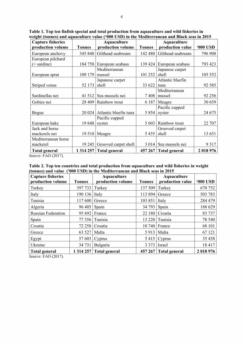
2. CAPTURE FISHERIES AND AQUACULTURE IN THE MEDITERRANEAN In the Mediterranean and Black seas2, capture fisheries production in 2013 was 1.3 million tonnes, of which, 1 113 thousand tonnes were fish, 138 thousand tonnes were molluscs and 61 thousand tonnes were crustaceans (FAO, 2017). The main capture species in 2015 (see Table 1) are European anchovy, which represents 26 percent of the total production, European pilchard (14 percent), European sprat (8 percent) and striped venus (4 percent). While quantity data are available for both aquaculture and capture fisheries, value data are only available for aquaculture. Marine aquaculture production in the Mediterranean and Black seas reached 457 thousand tonnes in 2015, with 305 thousand tonnes coming from fish and 152 from molluscs (FAO, 2017). Marine aquaculture production in the Mediterranean and Black seas is concentrated on gilthead seabream and European seabass, and the two species combined represent 62 percent in weight and 79 percent in value of the total Mediterranean and Black seas aquaculture production. Other farmed species in terms of quantity are Mediterranean mussel (22 percent) and Japanese carpet shell (7 percent), both of which represent 5 percent in terms of value (see Table 1). The main fishing nations in the Mediterranean and Black seas are Turkey, accounting for 30 percent of the total catches, followed by Italy (14 percent), Tunisia (9 percent), Algeria (7 percent) and the Russian Federation (7 percent) (see Table 2). Marine aquaculture production is more concentrated, with Turkey responsible for 30 percent of the total quantity produced followed by Italy (25 percent), Greece (23 percent) and Spain (8 percent) (see Table 2).
2 The Mediterranean Sea is located between Europe and Africa, as well as Asia in the East. It is connected to the Atlantic Ocean through the 14-km-wide Gibraltar Strait and is almost completely enclosed by land: on the north by southern Europe and Anatolia, on the south by North Africa, and on the east by the Levant. The Mediterranean Sea covers an area of over 2.5 million square km (950 000 square miles). The Black Sea is a sea between southeastern Europe and western Asia. It is bounded by Europe, Anatolia and the Caucasus. The Black Sea is an inland sea connected to the Marmara Sea by the narrow and shallow Bosporus Strait, while the Strait of Dardanelles further connects the Marmara Sea to the Aegean Sea region of the Mediterranean Sea. The Black Sea is also connected to the Sea of Azov by the Strait of Kerch. The Black Sea (not including the Sea of Azov) covers an area of 436 400 square km (168 500 square miles). Marine biodiversity differs significantly between the Mediterranean Sea and the Black Sea, in great part due to the Black Sea’s reduced salinity. In the Mediterranean Sea there are two to five times more species in various benthic taxa than in the Black Sea. There are twice as many macroalgal varieties in the Medierranean as in the Black Sea, and planktonic biodiversity is about 1.5 times higher. In the Black Sea there are no corals, no octopuses or squids, no seastars or sea urchins (of all the echinoderms, only several small ophiuran and holothurian species are adapted to the Black Sea’s habitat).
4
Table 1. Top ten finfish special and total production from aquaculture and wild fisheries in weight (tonnes) and aquaculture value (‘000 USD) in the Mediterranean and Black seas in 2015
Capture fisheries production volume Tonnes
Aquaculture production volume Tonnes
Aquaculture production value ‘000 USD
European anchovy 345 840 Gilthead seabream 142 480 Gilthead seabream 796 908 European pilchard (= sardine) 184 758 European seabass 139 424 European seabass 793 423
European sprat 109 179 Mediterranean mussel 101 252
Japanese carpet shell 105 552
Striped venus 52 173 Japanese carpet shell 33 622
Atlantic bluefin tuna 92 585
Sardinellas nei 41 512 Sea mussels nei 7 408 Mediterranean mussel 92 256
Gobies nei 28 409 Rainbow trout 6 187 Meagre 30 659
Bogue 20 024 Atlantic bluefin tuna 5 854 Pacific cupped oyster 24 675
European hake 19 648 Pacific cupped oyster 5 603 Rainbow trout 22 707
Jack and horse mackerels nei 19 510 Meagre 5 435
Grooved carpet shell 13 651
Mediterranean horse mackerel 19 245 Grooved carpet shell 3 014 Sea mussels nei 9 317
Total general 1 314 257 Total general 457 267 Total general 2 018 976 Source: FAO (2017). Table 2. Top ten countries and total production from aquaculture and wild fisheries in weight (tonnes) and value ('000 USD) in the Mediterranean and Black seas in 2015 Capture fisheries production volume Tonnes
Aquaculture production volume Tonnes
Aquaculture production value ‘000 USD
Turkey 397 733 Turkey 137 509 Turkey 670 752
Italy 190 136 Italy 113 894 Greece 503 783
Tunisia 117 600 Greece 103 851 Italy 284 479
Algeria 96 405 Spain 34 793 Spain 188 629
Russian Federation 95 692 France 22 180 Croatia 83 737
Spain 77 356 Tunisia 13 220 Tunisia 78 540
Croatia 72 258 Croatia 10 740 France 68 101
Greece 63 527 Malta 5 913 Malta 67 121
Egypt 57 603 Cyprus 5 415 Cyprus 35 458
Ukraine 34 731 Bulgaria 3 373 Israel 18 417
Total general 1 314 257 Total general 457 267 Total general 2 018 976 Source: FAO (2017).
5
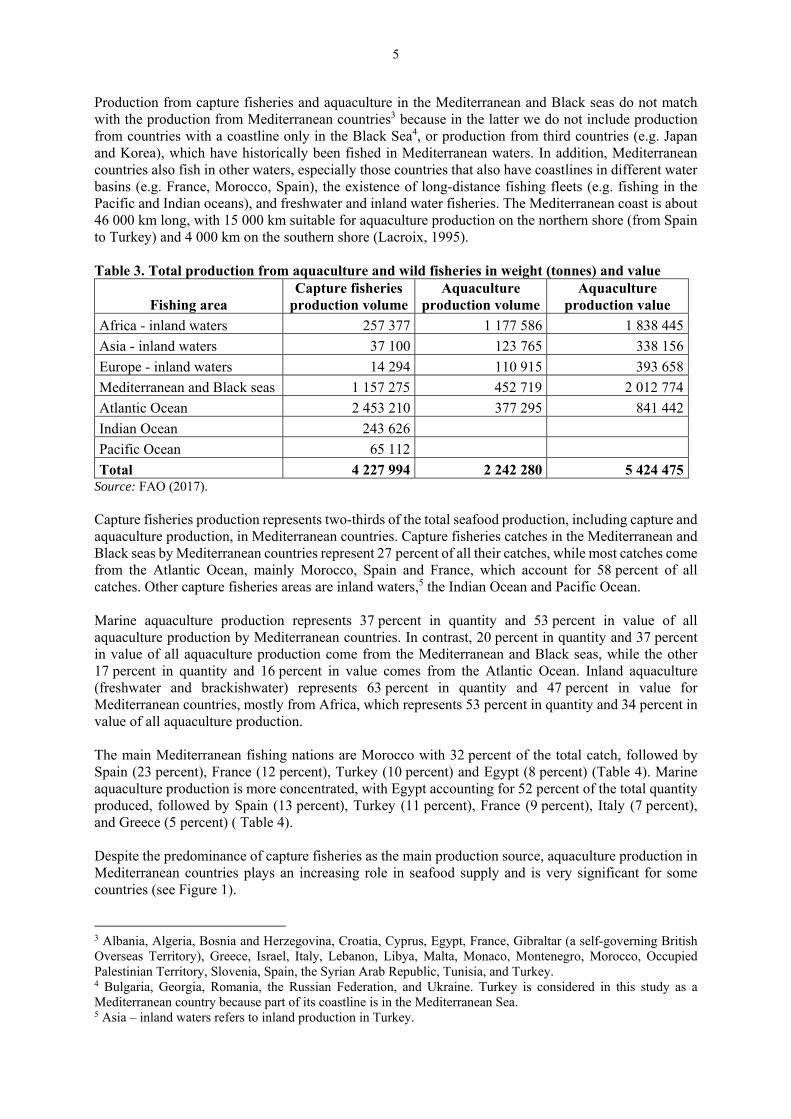
Production from capture fisheries and aquaculture in the Mediterranean and Black seas do not match with the production from Mediterranean countries3 because in the latter we do not include production from countries with a coastline only in the Black Sea4, or production from third countries (e.g. Japan and Korea), which have historically been fished in Mediterranean waters. In addition, Mediterranean countries also fish in other waters, especially those countries that also have coastlines in different water basins (e.g. France, Morocco, Spain), the existence of long-distance fishing fleets (e.g. fishing in the Pacific and Indian oceans), and freshwater and inland water fisheries. The Mediterranean coast is about 46 000 km long, with 15 000 km suitable for aquaculture production on the northern shore (from Spain to Turkey) and 4 000 km on the southern shore (Lacroix, 1995). Table 3. Total production from aquaculture and wild fisheries in weight (tonnes) and value
Fishing area Capture fisheries
production volume Aquaculture
production volume Aquaculture
production value
Africa - inland waters 257 377 1 177 586 1 838 445
Asia - inland waters 37 100 123 765 338 156
Europe - inland waters 14 294 110 915 393 658
Mediterranean and Black seas 1 157 275 452 719 2 012 774
Atlantic Ocean 2 453 210 377 295 841 442
Indian Ocean 243 626
Pacific Ocean 65 112
Total 4 227 994 2 242 280 5 424 475 Source: FAO (2017). Capture fisheries production represents two-thirds of the total seafood production, including capture and aquaculture production, in Mediterranean countries. Capture fisheries catches in the Mediterranean and Black seas by Mediterranean countries represent 27 percent of all their catches, while most catches come from the Atlantic Ocean, mainly Morocco, Spain and France, which account for 58 percent of all catches. Other capture fisheries areas are inland waters,5 the Indian Ocean and Pacific Ocean. Marine aquaculture production represents 37 percent in quantity and 53 percent in value of all aquaculture production by Mediterranean countries. In contrast, 20 percent in quantity and 37 percent in value of all aquaculture production come from the Mediterranean and Black seas, while the other 17 percent in quantity and 16 percent in value comes from the Atlantic Ocean. Inland aquaculture (freshwater and brackishwater) represents 63 percent in quantity and 47 percent in value for Mediterranean countries, mostly from Africa, which represents 53 percent in quantity and 34 percent in value of all aquaculture production. The main Mediterranean fishing nations are Morocco with 32 percent of the total catch, followed by Spain (23 percent), France (12 percent), Turkey (10 percent) and Egypt (8 percent) (Table 4). Marine aquaculture production is more concentrated, with Egypt accounting for 52 percent of the total quantity produced, followed by Spain (13 percent), Turkey (11 percent), France (9 percent), Italy (7 percent), and Greece (5 percent) ( Table 4). Despite the predominance of capture fisheries as the main production source, aquaculture production in Mediterranean countries plays an increasing role in seafood supply and is very significant for some countries (see Figure 1). 3 Albania, Algeria, Bosnia and Herzegovina, Croatia, Cyprus, Egypt, France, Gibraltar (a self-governing British Overseas Territory), Greece, Israel, Italy, Lebanon, Libya, Malta, Monaco, Montenegro, Morocco, Occupied Palestinian Territory, Slovenia, Spain, the Syrian Arab Republic, Tunisia, and Turkey. 4 Bulgaria, Georgia, Romania, the Russian Federation, and Ukraine. Turkey is considered in this study as a Mediterranean country because part of its coastline is in the Mediterranean Sea. 5 Asia – inland waters refers to inland production in Turkey.

6
Gibraltar and Monaco are not further included in the analysis due to their low total production and consumption, which is the result of their small populations of almost 29 000 and 38 000, respectively. Table 4. Top ten countries and total production from aquaculture and wild fisheries in weight (tonnes) and value ('000 USD) in the Mediterranean and Black seas in 2015
Country Total seafood
production Capture fisheries
production volume Aquaculture
production volume Aquaculture
production value
Albania 7 875 6 280 1 595 8 723
Algeria 97 738 96 405 1 333 4 398 Bosnia and Herzegovina 4 756 305 4 451 13 929
Croatia 88 274 72 702 15 572 92 980
Cyprus 6 954 1 495 5 459 35 844
Egypt 1 518 944 344 113 1 174 831 1 831 035
France 712 013 505 213 206 800 817 037
Gibraltar 1 1 0 0
Greece 171 310 65 192 106 118 513 903
Israel 22 933 2 078 20 855 87 593
Italy 346 961 198 198 148 763 406 423
Lebanon 4 763 3 638 1 125 3 465
Libya 26 012 26 002 10 20
Malta 8 351 2 438 5 913 67 121
Monaco 1 1 0 0
Montenegro 2 300 1 487 813 3 178
Morocco 1 370 981 1 369 931 1 050 6 129 Occupied Palestinian Territory 3 503 3 227 276 2 590
Slovenia 1 951 343 1 607 4 729
Spain 1 265 453 975 632 289 821 509 014 Syrian Arab Republic 6 600 4 100 2 500 8 196
Tunisia 133 217 118 792 14 425 80 622
Turkey 670 873 431 909 238 964 927 546
Totals 6 471 760 4 229 481 2 242 280 5 424 475 Source: FAO (2017).

7
Figure 1. Capture and aquaculture production shares of the total seafood production by Mediterranean country (2015)
Source: authors’ elaboration of FAO data (2017).
Mediterranean countries are net importers of seafood products, with imports being more than double that of exports. Indeed, in 2013, Mediterranean countries imported almost 4.8 million tonnes of seafood products (corresponding to about 6.8 million tonnes in live weight) valued at USD 22.0 billion, compared with the 2.4 million tonnes (equivalent to more than 2.5 million tonnes in live weight) exported valued at USD 10.5 billion (FAO, 2017). Only Morocco exported more in quantity than it imported; while in monetary terms, exports from Morocco, Croatia, Tunisia, Greece, the Turkey, Albania and Malta were more valuable than imports in 2013 (see Figure 2) (FAO, 2017). There has been a significant increase in external trade (imports and exports) during recent years. Countries such as Egypt, Croatia, Lebanon or the Syrian Arab Republic have experienced an important increase (Franquesa, Oliver and Basurco, 2008). Figure 2. Import and export shares in quantity and value by Mediterranean country (2013)
Source: authors’ elaboration of FAO data (2017).
0
20
40
60
80
100
Aquaculture
Capture
0
20
40
60
80
100%
Import Q
Export Q
Import V
Export V

8
In fact, external trade is the main seafood supply for most Mediterranean countries. External trade (imports and exports) represents 50 percent or more of the total seafood supply for Bosnia and Herzegovina, Cyprus, France, Israel, Italy, Lebanon, Libya, Malta, Montenegro, Occupied Palestinian Territory, Slovenia, Spain and the Syrian Arab Republic in 2013 (see Figure 3). Figure 3. Capture, aquaculture and external trade shares of the total seafood supply by Mediterranean country (2013)
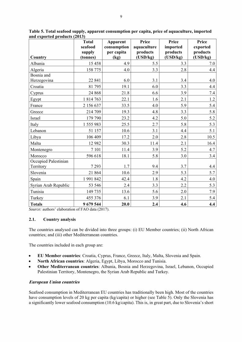
Source: authors’ elaboration of FAO data (2017). Total seafood supply, or apparent consumption6, in Mediterranean countries was almost 9.7 million tonnes in live weight in 2013 (see Table 5) (FAO, 2017). The countries with the largest seafood consumption are France, Spain, the Egypt and Italy; these four countries consume 78 percent of all seafood in Mediterranean countries. While seafood consumed per capita (apparent consumption per capita7) is led by Spain, followed by France, Malta, Italy, Israel, Egypt and Cyprus (see Table 5). Average seafood consumption per capita varies from the 42.4 kg per person (kg/person) in Spain to the 1.7 kg/person in the Occupied Palestinian Territory. The total population of Mediterranean countries was 484 million people in 2013 (FAO, 2017).
6 Apparent consumption is defined as the sum of capture fisheries production, aquaculture production and imports volume minus the exports volume. 7 Apparent consumption divided by the population.
0
20
40
60
80
100
External trade
Aquaculture
Capture
9
Table 5. Total seafood supply, apparent consumption per capita, price of aquaculture, imported and exported products (2013)
Country
Total seafood supply
(tonnes)
Apparent consumption
per capita (kg)
Price aquaculture
products (USD/kg)
Price imported products (USD/kg)
Price exported products (USD/kg)
Albania 15 458 4.9 5.5 3.3 7.0
Algeria 158 775 4.0 3.3 2.8 4.4 Bosnia and Herzegovina 22 841 6.0 3.1 3.4 4.0
Croatia 81 795 19.1 6.0 3.3 4.4
Cyprus 24 868 21.8 6.6 3.9 7.4
Egypt 1 814 763 22.1 1.6 2.1 1.2
France 2 156 637 33.5 4.0 5.9 5.4
Greece 214 709 19.3 4.8 3.3 5.8
Israel 179 790 23.2 4.2 5.0 5.2
Italy 1 555 983 25.5 2.7 5.8 5.3
Lebanon 51 157 10.6 3.1 4.4 5.1
Libya 106 409 17.2 2.0 2.8 10.5
Malta 12 982 30.3 11.4 2.1 16.4
Montenegro 7 101 11.4 3.9 5.2 4.7
Morocco 596 618 18.1 5.8 3.0 3.4 Occupied Palestinian Territory 7 293 1.7 9.4 3.7 4.4
Slovenia 21 864 10.6 2.9 5.3 5.7
Spain 1 991 842 42.4 1.8 4.2 4.0
Syrian Arab Republic 53 546 2.4 3.3 2.2 5.3
Tunisia 149 735 13.6 5.6 2.0 7.9
Turkey 455 376 6.1 3.9 2.1 5.4
Totals 9 679 544 20.0 2.4 4.6 4.4 Source: authors’ elaboration of FAO data (2017). 2.1. Country analysis
The countries analysed can be divided into three groups: (i) EU Member countries; (ii) North African countries; and (iii) other Mediterranean countries. The countries included in each group are: EU Member countries: Croatia, Cyprus, France, Greece, Italy, Malta, Slovenia and Spain. North African countries: Algeria, Egypt, Libya, Morocco and Tunisia. Other Mediterranean countries: Albania, Bosnia and Herzegovina, Israel, Lebanon, Occupied
Palestinian Territory, Montenegro, the Syrian Arab Republic and Turkey. European Union countries Seafood consumption in Mediterranean EU countries has traditionally been high. Most of the countries have consumption levels of 20 kg per capita (kg/capita) or higher (see Table 5). Only the Slovenia has a significantly lower seafood consumption (10.6 kg/capita). This is, in great part, due to Slovenia’s short

10
coastline (46 km), a population of two million people, and total area of more than 20 000 km2. Most of Slovenia’s seafood supply comes from imports. France, Greece, Italy and Spain are important fishing nations with high levels of seafood consumption. Italy complements its Mediterranean catches mainly with high levels of imports. France and Spain, together with high levels of imports, have their most important fishery grounds in the Atlantic Ocean, while Greece also has a significant part of its seafood supply coming from aquaculture. French, Italian and Spanish import prices are higher than those for exports, while Greek export prices are higher, in great part because of exporting high-value aquaculture products (gilthead seabream and European seabass). Greece and Turkey, are the main producers of gilthead seabream and European seabass. Greek production of gilthead seabream and European seabass in 2015 is estimated to be 47 000 tonnes and 35 000 tonnes, respectively. Other significant productions are Mediterranean mussel with almost 19 000 tonnes and rainbow trout at almost 2 000 tonnes. Low average aquaculture prices in Spain can be explained because the country produces a large volume of mussels (225 000 tonnes in 2015) that are relatively cheap (USD 0.57/kg). Other important aquaculture products in Spain are gilthead seabream and European seabass at 19 000 tonnes and 16 000 tonnes, rainbow trout also at 16 000 tonnes and turbot at more than 7 000 tonnes. It should be noted that almost three-quarters of the gilthead seabream and European seabass production takes place in the Mediterranean, while the majority of mussel and turbot production takes place in Atlantic waters. Similarly, most aquaculture production in France comes from Atlantic waters. Main species farmed in France are Pacific cupped oyster with an estimated production in 2015 of 75 000 tonnes, blue mussel at 61 000 tonnes, rainbow trout at more than 36 000 tonnes, and Mediterranean mussel at 14 000 tonnes. In the Mediterranean Sea, the main species produced are Mediterranean mussel at almost 14 000 tonnes and Pacific cupped oyster at 5 000 tonnes. Gilthead seabream and European seabass production is relatively small compared with other countries in the Mediterranean, at about 2 000 tonnes each. Italian marine aquaculture takes place in the Mediterranean Sea. The main aquaculture species are Mediterranean mussel at 64 000 tonnes, Japanese carpet shell at almost 34 000 tonnes, rainbow trout at more than 31 000 tonnes, gilthead seabream at almost 7 000 tonnes and European seabass at almost 6 000 tonnes. In Cyprus and Malta, the main seafood supply consists of imports; while for Croatia imports play a tiny role and its main seafood supply is from capture fisheries. Malta’s aquaculture and export prices are the highest in the Mediterranean (see Table 5), which can be explained by the cultivation and its later export of Atlantic bluefin tuna (Thunnus thynnus). Farmed Atlantic bluefin tuna production in Malta was more than 3 000 tonnes in 2015, while gilthead seabream production was almost 2 500 tonnes. In Cyprus, gilthead seabream and European seabass productions were almost 4 000 tonnes and almost 2 000 tonnes, respectively. In Croatia, the main species produced in 2015 were European seabass and gilthead seabream at more than 4 000 tonnes each, common carp at more than 3 000 tonnes, and Atlantic bluefin tuna at more than 1 000 tonnes (capture catches of Atlantic bluefin tuna were 500 tonnes). North African countries Seafood consumption varies largely by country. For example, Egypt has a high consumption at more than 22 kg/capita, while Libya, Morocco and Tunisia have consumption rates above 10 kg/capita, and Algeria below 5 kg/capita. For the Syrian Arab Republic and Libya, imports are the main source of seafood. For Algeria and Morocco capture fisheries are the main source, while Egypt, aquaculture is the main source of seafood. The main seafood production in most North African countries (Algeria, Libya, Morocco and Tunisia) comes from capture fisheries. Indeed, these four countries have the largest share of capture fisheries in terms of total seafood production. In 2015, Tunisia produced 10 000 tonnes of gilthead seabream and almost 3 000 tonnes of European seabass; the Syrian Arab Republic produced more than 1 000 tonnes

11
of common carp and almost 1 000 tonnes of blue tilapia; Algeria produced almost 1 000 tonnes of cyprinids, while the production of other species was very limited. Egypt is an exception, and inland aquaculture plays a main role in seafood production. Most of Egypt’s aquaculture production is from the brackishwater areas of its delta lakes and lagoons in the north of the country (Monfort, 2007). Egypt is the largest producer of tilapia in the Mediterranean; in fact, the main species produced is Nile tilapia (Oreochromis niloticus) at 876 000 tonnes, followed by mullet (157 000 tonnes), other cyprinids (65 000 tonnes), common carp (Cyprinus carpio) at 30 000 tonnes, gilthead seabream (16 000 tonnes) and European seabass (14 000 tonnes). The Egyptian volume of exports represents only 7 percent of the imports in volume and 4 percent in value. Tilapia sales, as well as most of the Egyptian production, have been traditionally mostly restricted to local markets due to its high production costs relative to other producer countries as well as food safety concerns from the EU and the USA (Feidi, 2004; Macfadyen, Nasr-Allah and Dickson, 2012; Goulding and Kamel, 2013). In addition, Norman-López and Bjørndal (2009) found that prices of frozen tilapia fillets in the Egypt are not related to other tilapia prices in international markets. On the other hand, Morocco’s seafood production comes mostly from capture fisheries (aquaculture represented less than the 0.1 percent of the total seafood production in 2015). Most of the landings of capture fisheries come from Atlantic waters (98 percent), while landings from the Mediterranean Sea account for less than 2 percent. Moreover, Morocco is the only net exporter (by volume) country in the whole region. The main products exported are European sardines and anchovies (prepared or preserved), octopus, frozen cuttlefish, frozen shrimps and prawns, and fresh, chilled or boiled common crangon shrimps (FAO, 2017). Libya’s high export prices (see Table 5) are because most exports from Libya are of fresh and frozen wild-caught Atlantic bluefin tuna. Other Mediterranean countries The “other” group of Mediterranean countries (i.e., Albania, Bosnia and Herzegovina, Israel, Lebanon, Montenegro, the Occupied Palestinian Territory, the Syrian Arab Republic and Turkey) represent a very heterogeneous set of countries. This group of countries is characterised by low to medium seafood consumption per capita: 1.7 kg/capita in the Occupied Palestinian Territory, 2.4 kg/capita in the Syrian Arab Republic, 11.4 kg/capita in Montenegro and 23.2 kg/capita in Israel. In Lebanon, Israel, the Occupied Palestinian Territory, the Syrian Arab Republic, Bosnia and Herzegovina, and Montenegro, more than 50 percent of the seafood supply comes from imports. In Albania, both imports and capture fisheries play a key role in the supply of seafood. While capture fisheries are the main source of seafood in Turkey, aquaculture production is also important, especially as a key source of exports. The main species cultured in Turkey are rainbow trout at almost 107 000 tonnes, European seabass at 75 000 tonnes, and gilthead seabream at almost 52 000 tonnes in 2015, with all these species showing an increasing production trend. The main species cultured in other Mediterranean countries are: 1) in Israel, 8 000 tonnes of tilapias, 4 000 tonnes of common carp, more than 3 000 tonnes of flathead grey mullet, and almost 2 000 tonnes of gilthead seabream; in Bosnia and Herzegovina, more than 3 000 tonnes of rainbow trout; in the Syrian Arab Republic, more than 1 000 tonnes of common carp and almost 1 000 tonnes of blue tilapia; and in Lebanon, 1 000 tonnes of rainbow trout.

12
2.2. Gilthead seabream and European seabass Gilthead seabream (Sparus aurata) and European seabass (Dicentrarchus labrax)8 are the most commonly produced species in the Mediterranean and Black seas, at 282 000 tonnes and USD 1.59 billion in 2015 (FAO, 2017).9 Gilthead seabream and European seabass represent 62 percent in quantity and 79 percent in value of all aquaculture production in the Mediterranean basin. Wild gilthead seabream and European seabass at the ex-vessel market
© FAO/J. Guillen at the Palermo fish market.
More than 95 percent of the world gilthead seabream and European seabass production comes from aquaculture, and 97 percent of the world gilthead seabream and European seabass production comes from Mediterranean countries, and includes inland production. The main producers are Turkey and Greece, while the main consumers are Spain, France, Italy, Greece and Turkey (see Tables 6 and 7). The evolution of the gilthead seabream aquaculture production and European seabass aquaculture production presents many similarities (see Figure 4). Significant levels of European seabass and gilthead seabream production did not start until the second half of the 1980s and early 1990s even though the first efforts to breed European seabass and gilthead seabream took place in France and Italy in the late 1970s and early 1980s, initially in government research laboratories and increasingly in the private sector (University of Stirling, 2004). The principal reason for the slow initial development of the industry was the difficulty in producing large quantities of good quality fry, and the complexity in obtaining licences (University of Stirling, 2004). The production increase from the late 1980s onwards was the result of improvements at hatcheries that led to an increase in the supply of juveniles.
8 The gilthead seabream (Sparus aurata) is a fish of the Sparidae family (bream) commonly found throughout the Mediterranean and along the northeastern Atlantic coasts from the United Kingdom to the Canary Islands. It can live in marine waters as well as in the brackishwaters of coastal lagoons. It has an oval-shaped body that is rather deep and compressed. It is silvery grey with a golden frontal band between the eyes and edged by two dark areas. It commonly reaches about 35 centimetres in length, but may reach up to 70 cm and weigh up to about 17 kg. It is the only species of sea bream that is currently farmed on a large scale. Farmed seabream can reach the first commercial size of 350–400 g in about one to one and a half years. European seabass (Dicentrarchus labrax) is common throughout the Mediterranean, the Black Sea and the northeastern Atlantic from Norway to Senegal. It inhabits coastal waters as well as brackishwaters to a depth of 100 metres. It has a rather elongated body, and is a silvery grey colour that turns bluish on the back. It commonly reaches about 50 cm in length, but may reach up to 100 cm and weigh up to about 12 kg. Farmed seabass are generally harvested when they weigh 300–500 g, which takes from a year and a half to two years, depending on water temperature. Both, European seabass and gilthead seabream are mostly cultivated in floating cages, and are almost always sold as fresh or chilled as a whole-portion-sized fish. 9 Not considering inland productions.

13
Table 6. Production evolution of farmed gilthead seabream (Sparus aurata) by main producer countries in 2015
Year
Country 1980 1985 1990 1995 2000 2005 2010 2011 2012 2013 2014 2015
Turkey 1 031 4 847 15 460 28 334 28 157 32 187 30 743 35 701 41 873 51 844
Greece 7 1 598 9 387 38 587 43 829 57 204 51 308 53 459 55 751 50 688 47 008
Egypt 1 062 8 862 4 398 15 065 14 155 14 806 14 537 16 967 16 092
Spain 127 565 2 706 8 242 15 433 20 358 15 118 16 607 18 897 16 915 16 005
Tunisia 5 85 160 409 576 2 296 4 184 5 273 8 475 8 124 10 216
Italy 250 360 850 3 200 6 000 6 914 6 260 5 508 5 400 5 400 6 830 6 800
Croatia 90 800 1 000 2 400 1 719 2 173 2 978 3 655 4 075
Cyprus 37 223 1 384 1 465 2 807 3 056 3 126 3 795 2 919 3 656
Saudi Arabia 1 300 1 453 1 648 1 825 1 685 3 057
Malta 550 1 512 540 1 755 1 082 2 604 2 550 2 704 2 337
Overall total 257 564 4 570 24 481 87 303 110 755 142 306 134 337 141 999 157 775 159 819 166 794 Source: FAO (2017). Table 7. Production evolution of farmed European seabass (Dicentrarchus labrax) by main producer countries in 2015
Year
Country 1980 1985 1990 1995 2000 2005 2010 2011 2012 2013 2014 2015
Turkey 102 2 773 17 877 37 490 50 796 47 013 65 512 67 913 74 653 75 164
Greece 5 60 1 952 9 539 26 653 30 959 39 884 37 089 35 805 34 920 32 142 35 382
Spain 29 31 461 1 837 5 713 11 491 17 548 14 455 14 945 16 722 18 600
Egypt 755 10 031 4 192 16 306 17 714 13 798 12 328 15 167 14 343
Italy 120 340 1 050 3 600 8 100 6 262 6 457 6 672 6 896 6 330 5 724 5 800
Croatia 247 1 300 2 000 2 800 2 775 2 453 2 826 3 215 4 488
Tunisia 15 283 230 202 633 1 466 2 832 1 999 1 968 1 869 2 802
France 70 300 2 656 3 020 3 913 2 337 2 452 2 321 2 428 2 400 2 400
Cyprus 1 15 99 299 583 1 198 1 495 1 100 1 422 1 817 1 726
Albania 135 170 170 170 129 392
Overall total 130 581 3 921 22 263 70 694 95 044 134 328 137 276 146 022 146 771 155 509 162 399 Source: FAO (2017).

14
Figure 4. Total aquaculture production and price of gilthead seabream and European seabass (2015)
Source: authors’ elaboration of FAO data (2017). Prices of farmed gilthead seabream and European seabass achieved their minimum level in 2001 and 2002 (ex-farm prices for gilthead seabream and European seabass in 2002 reached EUR 3.9/kg and EUR 4.3/kg, respectively), due to major production increases from 2000. Prices often fell below the cost of production, resulting in a major crisis in the industry (Rad and Köksal, 2000; University of Stirling, 2004; Rad, 2007; Wagner and Young, 2009; STECF, 2014). This brought a rationalization of the industry and stabilization of prices at around EUR 5.5/kg.
0
2
4
6
8
10
12
14
16
18
0
20
40
60
80
100
120
140
160
1801990
1992
1994
1996
1998
2000
2002
2004
2006
2008
2010
2012
2014
USD/KgThousand tonnes
Bass Q
Bream Q
Bass P
Bream P

15
3. METHODOLOGY The development of prices over time provides important information on the relationship between products, as has been widely recognised by economists such as Cournot (1838), Marshall (1947) and Stigler (1969). Market integration analysis, using time series data for prices, has been used for a number of seafood products. It is particularly useful when there is the need to analyse a large number of products because demand analysis in such cases is not feasible (Asche, Gordon and Hannesson, 2004). Following Ravallion (1986), market integration is analysed by looking at whether prices of products are related over time, which allows the price adjustment between markets to occur over time. So, we investigated whether the price of a product (dependent variable P1) can be explained by the price evolution of another product (explanatory variable P2), as well as its own previous price evolution. The relationships between variables have typically been studied with ordinary least squares regression analysis. Such analysis can be used when variables (i.e. prices) are stationary10 (Squires, Herrick Jr. and Hastie, 1989; Asche, Gordon and Hannesson, 2004). However, many economic variables show trends, and so these are non-stationary. When non-stationary time series such as prices are used in a regression model, relationships that appear to be significant may emerge from unrelated variables. These are called spurious regressions. Therefore, the use of cointegration methodology is required to estimate real, long-run relationships between non-stationary variables (Ardeni, 1989; Whalen, 1990; Goodwin and Schroeder, 1991). Since most seafood prices have been found to be non-stationary, cointegration is the most commonly used empirical tool to test for market integration.11 The idea of cointegration is that even if two or more variables are non-stationary in their levels, linear combinations (so-called cointegration vectors), which are stationary, may exist (Engle and Granger, 1987). When cointegration is verified, the variables exhibit one or more long-run relationships. Variables may drift apart due to random shocks, sticky prices, and contracts in the short run, but in the long run, the economic processes force the variables back to their, long-run equilibrium path (Engle and Ganger, 1987). The economic interpretation of cointegration is that “if two (or more) series are linked to form an equilibrium relationship spanning the long-run, then even though the series themselves may contain stochastic trends (that makes them to be non-stationary) they will nevertheless move closely together over time and the difference between them will be stable (so stationary)” (Harris, 1995:22). Therefore, prices for products in the same market are part of a long-run equilibrium system, although significant short-run deviations from equilibrium conditions may still be observed due to stochastic supply and demand shocks. So, if the products are substitutes, there will be market forces working to re-equilibrate the price ratio after a shock occurs in the market. Thus, when cointegration is verified, it implies the existence of a stable long-run relationship between prices, from which it can be assumed that a price parity equilibrium condition exists, and consequently the variables form part of the same market (Asche, Steen and Salvanes, 1997). So, cointegration theory is consistent with Stigler and Sherwin’s (1985) market definition12 and the stochastic behaviour of prices. We, therefore, investigated the existence of relationships between price series using the Johansen cointegration test (Johansen, 1988, 1991; Johansen and Juselius, 1990). Determining the lag order, in order to take this into account in the model, is a key issue in cointegration. This happens because in order to apply cointegration, a series should be non-stationary; but the stationarity properties of a series can change with the number of lags considered as explanatory variables. In other words, test results on
10 A stationary time series is a sequence of measurements of the same variable collected over time whose statistical properties such as mean, variance, autocorrelation, etc. are all constant over time. 11 For recent examples see Nielsen et al., 2007; Norman-López and Asche, 2008; Nielsen, Smit and Guillen, 2009. 12 Stigler and Sherwin (1985) define substitute products as those which are “in the same market” and whose relative prices “maintain a stable ratio”.

16
whether a series is stationary changes with the number of lags considered as explanatory variables. The optimal number of lags for one series (e.g. found using a unit root test) may be different from the optimal number of lags for another series we want to compare. And these lag lengths may be different from the optimal number of lags when applying cointegration methodology. Thus, estimating the optimal number of lags for one series using a unit root test may be of little help initially. Moreover, different lag-length selection criteria often lead to different conclusions regarding the optimal number of lags that should be used. Meanwhile, the choice of the lag length can considerably affect the results of the cointegration analysis (Emerson, 2007). Therefore, we determined the number of lags using three different criteria: log likelihood Akaike information criteria Schwarz criteria Four different outcomes can be obtained from the cointegration tests of bivariate systems when estimating them for the number of lags obtained using the previous criteria: All tests show two cointegration equations. In this case, prices are stationary and cointegration
methodology cannot be applied. All tests show zero cointegration equations. Here, prices are not cointegrated, and consequently
products are not in the same market. All tests show one cointegration equation. There is a need to investigate the stationarity properties
of the series, and there are two options to do so. It could be that both series are non-stationary and they are cointegrated (i.e. are part of the same market), so there is only one cointegration equation. However, it is also possible that one of the series is stationary and the other one is non-stationary and, consequently, they are not cointegrated.
Outcomes from the tests report different numbers of cointegration equations, depending on the lag chosen. There is a need to investigate the stationarity properties of the series, and the results should be considered with caution.
When cointegration methodology cannot be applied (no cointegration equations are found), regressions and Granger causality tests (Granger, 1969) are used to investigate the relations between variables.

17
4. DATA In this section, the data used for the realization of this study are described. Wild and farmed seabream and seabass price data from Spain, France, Italy, Greece, Portugal and Turkey have been used for different levels in the market chain. The market stages analysed include wholesale, retail, together with the imports and exports. Other species with available price data for wild and farmed varieties, such as turbot, blackspot seabream, Atlantic cod, meagre, clams and mussels have been also analysed. Weekly data have been used when possible; if weekly data were not available, then monthly data were used. The most recent data available have been used, with price series starting no earlier than 2009 or 2010 and ending at the end of 2014 or in 2015. Longer price series are available for Spain’s Madrid and Barcelona wholesale markets, with series starting in 2003 and 2006, respectively. Unfortunately, all of the required price series to complete the market integration analysis for all Mediterranean countries are not available or do not cover a long enough time period. The use of cointegration methodology is very data demanding, requiring a large number of observations (close to 100 observations, depending on the characteristics of the series) in order to obtain robust results. In addition, in order to perform our study we required for each species analysed, disaggregated price data between farmed and wild origin fish. However, these data are rarely available, in part because: i) few countries collect and report detailed price data, and ii) there are few markets where both wild and farmed supplies of a species are present and properly differentiated. The price data used in this analysis are detailed by country. 4.1. Spain Weekly data for Madrid’s wholesale market (Mercamadrid) for the period 2003–14 (623 observations) for the species: gilthead seabream (Sparus aurata), fresh whole, wild and farmed; European seabass (Dicentrarchus labrax), fresh whole, wild and farmed; turbot (Scophthalmus maximus), fresh whole, wild and farmed; and sole (Solea spp.), fresh whole, wild and farmed, 2012–14 (141 observations). Figure 5. Weekly prices of wild and farmed gilthead seabream and European seabass in Mercamadrid (2003–14)
Source: Mercamadrid (2015).
0
5
10
15
20
25
30
35
40
1 25
49
73
97
121
145
169
193
217
241
265
289
313
337
361
385
409
433
457
481
505
529
553
577
601
€/kg
week
Bass_Wild
Bream_Wild
Bass_Farmed
Bream_Farmed

18
Weekly data for Barcelona’s wholesale market (Mercabarna) for the period 2006–14 (468 observations) for the species: gilthead seabream (Sparus aurata), fresh whole, wild and farmed; European seabass (Dicentrarchus labrax), fresh whole, wild and farmed; turbot (Scophthalmus maximus), fresh whole, wild and farmed; blackspot (red) seabream (Pagellus bogaraveo), fresh whole, wild and farmed; Atlantic cod (Gadus morhua), fresh whole, wild and farmed; clams (Venerupis spp.), fresh whole, wild and farmed; and meagre (Argyrosomus regius), fresh whole, wild and farmed. Figure 6. Weekly prices of wild and farmed gilthead seabream and European seabass in Mercabarna (2006–14)
Source: Mercabarna (2015). 4.2. France Weekly data for the Paris wholesale market (Rungis) for the period 2009–14 (313 observations): gilthead seabream (Sparus aurata), fresh whole 400–600 g, farmed; and European seabass (Dicentrarchus labrax), fresh whole 400–600 g, farmed.
0
5
10
15
20
25
30
35
40
1
19
37
55
73
91
109
127
145
163
181
199
217
235
253
271
289
307
325
343
361
379
397
415
433
451
€/kg
week
Bass_Wild
Bream_Wild
Bass_Farmed
Bream_Farmed

19
Figure 7. Weekly prices of farmed gilthead seabream and European seabass in Rungis (2009–14)
Source: EUMOFA (2015). Retail, weekly data for the period 2010 to mid-2015: European seabass (Dicentrarchus labrax), fresh whole, wild and farmed (114 and 257 observations,
respectively). Figure 8. Weekly prices of wild and farmed European seabass at the French retail level (2010 to mid-2015)
Source: EUMOFA (2015). 4.3. Italy Weekly data for Milano’s wholesale market for the period 2010–14 (225 observations) for the species: gilthead seabream (Sparus aurata), fresh whole, national and imported; and European seabass (Dicentrarchus labrax), fresh whole, national and imported.
0
1
2
3
4
5
6
7
8
9
10
1
14
27
40
53
66
79
92
105
118
131
144
157
170
183
196
209
222
235
248
261
274
287
300
313
€/kg
week
Bass_Farmed
Bream_Farmed
0
5
10
15
20
25
30
1
13
25
37
49
61
73
85
97
109
121
133
145
157
169
181
193
205
217
229
241
253
265
277
289
€/kg
week
Bass_Wild
Bass_Farmed

20
Figure 9. Weekly prices of national and imported gilthead seabream and European seabass in Milano wholesale market (2010–14)
Source: EUMOFA (2015). Weekly data for Rome’s wholesale market for the period 2010–14 for the species: gilthead seabream (Sparus aurata), fresh whole, national and imported (247 and 185 observations,
respectively); and European seabass (Dicentrarchus labrax), fresh whole, national and imported (151 and 182
observations, respectively). Figure 10. Weekly prices of national and imported gilthead seabream and European seabass in Rome wholesale market (2010–14)
Source: EUMOFA (2015). Retail, weekly data for the period from January 2013 to mid-2015 (125 observations): European seabass (Dicentrarchus labrax), fresh whole, farmed; gilthead seabream (Sparus aurata), fresh whole, farmed.
0
2
4
6
8
10
12
1
11
21
31
41
51
61
71
81
91
101
111
121
131
141
151
161
171
181
191
201
211
221
231
241
251
€/kg
week
Bass_imported
Bass_national
Bream_imported
Bream_national
0
2
4
6
8
10
12
14
16
1
11
21
31
41
51
61
71
81
91
101
111
121
131
141
151
161
171
181
191
201
211
221
231
241
251
€/kg
week
Bass_national
Bass_imported
Bream_national
Bream_imported

21
Figure 11. Weekly prices of farmed European seabass and gilthead seabream at the Italian retail level (2013 to mid-2015)
Source: EUMOFA (2015). 4.4. Portugal Retail, monthly data for the period from January 2010 to July 2015 (67 observations): European seabass (Dicentrarchus labrax), fresh whole, farmed; and gilthead seabream (Sparus aurata), fresh whole, farmed. Figure 12. Monthly prices of farmed European seabass and gilthead seabream at the Portuguese retail level (January 2010–July 2015)
Source: EUMOFA (2015).
0
2
4
6
8
10
12
14
1 6
11
16
21
26
31
36
41
46
51
56
61
66
71
76
81
86
91
96
101
106
111
116
121
€/kg
week
Bass_Farmed
Bream_Farmed
0
1
2
3
4
5
6
7
8
9
1 4 7 10 13 16 19 22 25 28 31 34 37 40 43 46 49 52 55 58 61 64 67
€/kg
month
Bass_Farmed
Bream_Farmed

22
4.5. Greece
Retail, monthly data for the period from November 2011 to July 2015 (34 observations): European seabass (Dicentrarchus labrax), fresh whole, wild and farmed; and gilthead seabream (Sparus aurata), fresh whole, wild and farmed. Figure 13. Monthly prices of wild and farmed European seabass and gilthead seabream at the Greek retail level (November 2011–July 2015)
Source: EUMOFA (2015). 4.6. Turkey Weekly prices of seabass imported into the EU from Turkey for the period January 2011 to April 2015 (225 observations):
European seabass (Dicentrarchus labrax), fresh whole, farmed.
0
5
10
15
20
25
30
1 3 5 7 9 11 13 15 17 19 21 23 25 27 29 31 33 35 37 39 41 43
€/kg
month
Bass_Wild
Bream_Wild
Bass_Farmed
Bream_Farmed

23
Figure 14. Weekly prices of farmed European seabass imports from Turkey to the European Union (January 2011–April 2015)
Source: EUMOFA (2015).
0
1
2
3
4
5
6
7
1
10
19
28
37
46
55
64
73
82
91
100
109
118
127
136
145
154
163
172
181
190
199
208
217
€/kg
week
Bass_Farmed

24
5. RESULTS In this section, we report on the market integration results obtained in this study. Full results are fully reported on in the Appendix. 5.1. Wild and farmed integration: Gilthead seabream and European seabass In this section, we summarize the market integration between wild and farmed conspecifics of gilthead seabream and European seabass. By analysing the market integration between wild and farmed gilthead seabream and European seabass it is possible to investigate whether prices are related and, consequently, to determine if wild and farmed products are considered the same product or substitutes. Table 8. Market integration results between wild and farmed conspecifics
Species Market Market level Period Market integration European seabass Madrid (Spain) Wholesale 2003–14 Potential/No European seabass Barcelona (Spain) Wholesale 2006–14 Potential European seabass France Retail 2009–14 Potential Gilthead seabream Madrid (Spain) Wholesale 2003–14 No Gilthead seabream Barcelona (Spain) wholesale 2006–14 Potential/No
The results show that there is no or limited market integration between wild and farmed conspecifics of gilthead seabream and European seabass. So, wild and farm varieties of gilthead seabream and European seabass are not (or very limited) price related. 5.2. Wild and farmed integration: Other species In this section, we analyse the market integration between wild and farmed conspecifics of species other than European seabass and gilthead seabream. Thus, this section analyses the market integration between wild and farmed conspecifics of species other than gilthead seabream and European seabass. Table 9. Market integration results between wild and farmed conspecifics other than seabass and seabream
Species Market Market level Period Market integration
Turbot (Scophthalmus maximus) Madrid (Spain) wholesale 2003–14 No Sole (Solea spp.) Madrid (Spain) wholesale 2012–14 No Turbot (Scophthalmus maximus) Barcelona (Spain) wholesale 2006–14 No Blackspot (red) seabream (Pagellus bogaraveo)
Barcelona (Spain) wholesale 2006–14 Yes
Atlantic cod (Gadus morhua) Barcelona (Spain) wholesale 2006–14 Yes Clams (Venerupis spp.) Barcelona (Spain) wholesale 2006–14 No Meagre (Argyrosomus regius) Barcelona (Spain) wholesale 2006–14 No
Therefore, the results show that there is no market integration between wild and farmed conspecifics for turbot (Scophthalmus maximus), sole (Solea spp.), and meagre (Argyrosomus regius), while there is market integration between wild and farmed conspecifics for blackspot (red) seabream (Pagellus bogaraveo) and Atlantic cod (Gadus morhua). 5.3. Species integration: Seabream and seabass In this section, we explore whether gilthead seabream and European seabass are integrated into the market and this includes whether seabream and seabass can be considered substitutes.

25
Table 10. Species integration results Species Market Market
level Period Market
integration European seabass - gilthead seabream
Wild Madrid (Spain) wholesale 2003–14 No
European seabass - gilthead seabream
Wild Barcelona (Spain) wholesale 2006–14 Yes
European seabass - gilthead seabream
Farmed Madrid (Spain) wholesale 2003–14 Yes
European seabass - gilthead seabream
Farmed Barcelona (Spain) wholesale 2006–14 No
European seabass - gilthead seabream
Farmed Paris (France) wholesale 2009–14 No
European seabass - gilthead seabream
Farmed Italy retail 2013–15 No
European seabass - gilthead seabream
Farmed Portugal retail 2010–15 No
The results show that there is no market integration between gilthead seabream and European seabass in French, Italian and Portuguese markets, and only partly in the Spanish market. Market integration (i.e. prices moving together overtime) between farmed gilthead seabream and European seabass has been found at the Madrid wholesale market, and between wild gilthead seabream and European seabass at the Barcelona wholesale market. 5.4. Geographical integration In this section, we analyse the geographical component of the market integration of different wild and farmed species. Thus, the investigation focuses on whether the price of seabream and seabass in different geographical markets move together or are independent.

26
Table 11. Geographical market integration results for different wild and farmed species Species Market Market level Period Market
integration European seabass Wild Madrid -
Barcelona (Spain) wholesale 2006–14 Yes
European seabass Farmed Madrid - Barcelona (Spain)
wholesale 2006–14 No
European seabass Farmed Madrid (Spain) - Paris (France)
wholesale 2009–14 Uncertain/No
European seabass Farmed Barcelona (Spain) - Paris (France)
wholesale 2009–14 Uncertain
European seabass Farmed Turkey - Madrid (Spain)
Imports - wholesale
2011–14 Uncertain
European seabass Farmed Turkey - Barcelona (Spain)
Imports - wholesale
2011–14 No
European seabass Farmed Turkey - Paris (France)
Imports - wholesale
2011–14 No
Gilthead seabream Wild Madrid - Barcelona (Spain)
wholesale 2006–14 No
Gilthead seabream Farmed Madrid - Barcelona (Spain)
wholesale 2006–14 No
Gilthead seabream Farmed Madrid (Spain) -Paris (France)
wholesale 2009–14 No
Gilthead seabream Farmed Barcelona (Spain) Paris (France)
wholesale 2009–14 No
Turbot (Scophthalmus maximus)
Wild Madrid - Barcelona (Spain)
wholesale 2006–14 No
Turbot (Scophthalmus maximus)
Farmed Madrid - Barcelona (Spain)
wholesale 2006–14 Yes
The results show that, in general, there is no market integration between wild species from different markets; only market integration for wild European seabass has been found between the Barcelona and Madrid wholesale markets. Our results also show that market integration for farmed species is quite limited. Prices of farmed turbot (Scophthalmus maximus) in Barcelona and Madrid wholesale markets are integrated. In addition, the price relation between farmed European seabass in Barcelona and Madrid with farmed European seabass in Paris wholesale markets is uncertain in the best of the cases, and the perception is that they are not integrated. The same applies to farmed European seabass imported from Turkey into the EU, and farmed European seabass into the Madrid wholesale market. In fact, the results for market integration are not conclusive because market integration is denied or accepted depending on the number of lags chosen and the methodology applied.

27
6. DISCUSSION Bjørndal and Guillen (2016) analyse the literature on market interactions between wild and farmed fish. The literature on market competition between aquaculture and wild fish is based on a small number of species and markets. Studies concentrate on USA and EU markets, which are countries with the most traded species and the main consumer markets. Market integration studies initially focused on salmon, followed by an analysis of shrimp and tilapia, and recently of seabass and seabream (Bjørndal and Guillen, 2016). In particular, when it comes to the Mediterranean area, existing knowledge on competition interactions between wild and farmed species in the Mediterranean is limited, and based solely on studies investigating gilthead seabream (Sparus aurata) and European seabass (Dicentrarchus labrax). Most of the world’s production of gilthead seabream and European seabass comes from aquaculture (more than 95 percent). Gilthead seabream and European seabass are the most farmed species in the Mediterranean and Black sea. Gilthead seabream and European seabass represent 62 percent in quantity and 79 percent in value of all the marine aquaculture production in the Mediterranean and Black seas. Ninety-seven percent of the world’s gilthead seabream and European seabass production comes from Mediterranean countries. The main producers are Turkey and Greece, while the main consumers are the Spain, France, Italy, Greece and Turkey. The 5–10 EUR/kg retail price for seabass and seabream is far too high for a large proportion of the population living in southern Mediterranean countries (Monfort, 2007). The literature on market competition between farmed and wild gilthead seabream and European seabass has focused on the Spanish, French and Italian markets. These studies on competition interactions between wild and farmed species in Mediterranean countries are based on a very limited number of cases with no general trends detected. For the Spanish market, Alfranca et al. (2004) found that farmed gilthead seabream prices determine the evolution of wild gilthead seabream prices more directly than the wild gilthead seabream prices in the Barcelona wholesale market. However, Rodríguez et al. (2013) show that wild and farmed gilthead seabream are not integrated and, consequently, they are two heterogeneous products that are not substitutes in the Madrid wholesale market. More recently, Rodríguez Rodríguez and Bande Ramudo (2015) confirm that there is no integration between farmed and wild gilthead seabream, European seabass and turbot prices in the Madrid wholesale market. In French households, Regnier and Bayramoglu (2014) found that fresh, whole wild seabream and farmed gilthead seabream are partially integrated and that their price relationship is led by farmed seabream, while those for whole wild seabass and farmed European seabass are not integrated. On the other hand, Brigante and Lem (2001) concluded that wild and farmed conspecifics are not substitutes for gilthead seabream and European seabass in Italy. The results from this study confirm that there is no (or limited) market integration between wild and farmed conspecifics of gilthead seabream and European seabass for all cases analysed (Barcelona and Madrid wholesale markets, and French retail market). In addition, there is no market integration between wild and farmed turbot (Scophthalmus maximus) in the Barcelona and Madrid wholesale markets. There is also no market integration between wild and farmed conspecifics of sole (Solea spp.) in the Madrid wholesale market, clams (Venerupis spp.), and meagre (Argyrosomus regius) in the Barcelona wholesale market. In particular, farmed turbot represents almost 90 percent of all fresh turbot sold in the wholesale markets. In fact, domestic landings are minimal and perceived as a different product compared to farmed production. It is only in spring, when significant amounts of wild turbot are imported from the Netherlands that producers believe that wild turbot may compete with farmed turbot because in some years wild turbot can be cheaper than farmed. The results from this study confirm the differentiation between both products. On the other hand, farmed production of sole is quite small (about 1 percent of the total fresh sole sold), but the product is still under development and the marketed sizes of farmed sole are very small, sometimes even smaller than the minimum landing size of wild sole. So, the two

28
products can be easily differentiated in the market. Similarly, farmed meagre production suffers several technical issues and production is still limited. It is not a very popular species in Spain and consumption is quite concentrated in some areas in the south and east of the country. Meagre producers also failed in marketing it, by selling big fish that were 2–3 kg, which is not very convenient for household consumption. So, there is still work to do in technology and product development for farmed meagre. In the case of clam species, there is no market integration because wild and farmed species are different species and have different food uses. However, there is market integration between wild and farmed conspecifics for blackspot (red) seabream (Pagellus bogaraveo) and Atlantic cod (Gadus morhua). The existence of market integration between wild and farmed conspecifics for Atlantic cod can be explained because both products are imported and low volumes of farmed cod are sold. The supply of wild cod was expected to prevent opening an opportunity for aquaculture, but landings of wild cod recovered and marketing of fresh wild Norwegian cod improved, leading to renewed popularity of this species among Spanish consumers. This has led to the near collapse of the farmed cod industry. Only small-size farmed cod is sold and is less frequent than wild (farmed cod represented 22 percent of all fresh cod sold at the wholesale level). On the other hand, the existence of market integration between wild and farmed conspecifics for blackspot (red) seabream is a bit more unexpected. There is a very small number of farms producing blackspot (red) seabream and consequently its commercialization has been very reduced (representing only 2 percent of all fresh blackspot [red] seabream sold). Some retailers may even reject selling this product due to deformities in the black spot, which is not always as visible as it is in wild conspecifics. Thus, it could be possible to consider that because of the low volumes sold, the prices of farmed products follow similar trends as those of their wild conspecifics. This differentiation between farmed and wild-captured products can be explained, at least in part, by the negative perception aquaculture products have in comparison to wild fish in Spain, and southern Europe in general (Fernández-Polanco and Luna, 2010; Claret et al., 2012). Wild fish is always preferred to farmed fish among southern European consumers (Claret et al., 2012). Southern European consumers perceive farmed fish as being of lower quality and affected by more health and safety issues than wild fish (Kole, 2003; Verbeke et al., 2007; Fernández-Polanco and Luna, 2010). Farmed fish is also perceived as more processed or manipulated than those from the wild (Claret et al., 2012). This is translated into lower prices for farmed fish than for wild (capture) fish, and some fine restaurants only serve wild fish products, specifying this on their menus. Consequently, a share of the wild production will not enter into the more traditional market chains. This differentiation in favour of wild products occurs even if the aquaculture sector has the competitive advantage of having a higher degree of control over the production process and being able to deliver when requested, in the requested amount and at the requested quality (Asche, Guttormsen and Nielsen, 2013). The fact that most seabass and seabream are sold as fresh whole with head on, can help the market to differentiate between products. Consumers in southern European countries prefer whole fish. In contrast, Northern European consumers prefer filleted fish products. Despite this potential demand, the industrial production of fillets is minor. High production costs for large individual fish does not allow for competitive prices for seabass and seabream fillets and other value-added presentations (Monfort, 2007). Hence, the expansion of seabass and seabream in non-Mediterranean markets has been limited. The results show that there is no market integration between gilthead seabream and European seabass in French, Italian and Portuguese markets, and only partly in the Spanish market. Market integration between farmed gilthead seabream and European seabass has been found at the Madrid wholesale market, and between wild gilthead seabream and European seabass at the Barcelona wholesale market. While for the Spanish market, Alfranca et al. (2004) found that the influence on farmed and wild gilthead seabream (Sparus aurata) prices of wild sole, farmed Atlantic salmon (Salmo salar), farmed European seabass (Dicentrarchus labrax), and wild European seabass (Dicentrarchus labrax) prices is rather weak, with a low level of significance in the Barcelona wholesale market.
29
The evolution of gilthead seabream and European seabass aquaculture production presents many similarities. In fact, both species’ main production areas and techniques are the same, with many companies producing both species. So, it is not surprising that the price evolution for both products is similar (see Figure 4). Indeed, market integration (i.e. prices moving together over time) between farmed gilthead seabream and European seabass has been found at the Madrid wholesale market, and between wild gilthead seabream and European seabass at the Barcelona wholesale market. However, outcomes from this study also show that there is no market integration between gilthead seabream and European seabass in France, Italy and Portugal, and only partly in the Spanish market. These differences in the outcomes obtained could be based, at least in part, due to the different data sources employed, markets, and the time periods analysed. Fish markets are dynamic and are continuously changing, so results can be sensitive to the period investigated (Setälä et al., 2003). This made us work with the latest data available and with relatively similar time periods for all cases. Actually, Emerson (2007) demonstrated that the choice of lag length can drastically affect the results of the cointegration analysis. Moreover, different lag-length selection criteria often lead to a different conclusion regarding the optimal lag order that should be used. Therefore, in this study, we determined the number of lags using three different criteria: log likelihood, Akaike information criteria, and Schwarz criteria. This has led several times to contradictory results, depending on the number of lags chosen (i.e. depending on the criteria used). We have marked these cases as not conclusive or uncertain. In addition, regression methodology tends to be more accepting toward the relationship between variables than cointegration methodology, and regression methodology was fully applied in cases where market integration was found. This is extremely evident in those cases where the initial cointegration analysis showed that 0 lags was the preferred model. So, for example, the existence of market integration between gilthead seabream and European seabass in Spain cannot be fully assured. Finally, we have analysed the spatial or geographical market integration. The results show that, in general, there is no market integration between wild species from different markets; only market integration for wild European seabass has been found between the Barcelona and Madrid wholesale markets. This could be because the main supply in both markets comes from the same source: the Northeast Atlantic (FAO area 27). A higher degree of integration between markets for farmed species was expected because aquaculture products are more subject to competition; however, our results show that market integration for farmed species is also quite limited. Prices of farmed turbot (Scophthalmus maximus) in Barcelona and Madrid wholesale markets are integrated. Unfortunately, turbot price data are not available from other Mediterranean markets. The price relation between farmed European seabass in Barcelona and Madrid with the farmed European seabass Paris wholesale markets is uncertain in the best of cases, and the perception is that they are not integrated. The same applies to farmed European seabass imported from Turkey into the EU and farmed European seabass in the Madrid wholesale market. In fact, the results for market integration are not conclusive because market integration is denied or accepted, depending on the number of lags chosen and the methodology applied. These latter results are a bit surprising because we were expecting to find a higher level of market integration between markets for farmed seabream and seabass due to the high volumes of imports coming from Greece and Turkey arriving at the Spanish, French and Italian markets. These imports would lead the long-term price evolution of these products in the more local markets. However, we have only found partial evidence for European seabass. This outcome is difficult to explain and would require larger and better datasets before we could draw more irrefutable conclusions. For example, data are currently unavailable, or at least to the extent

30
necessary to do this kind of analysis, for southern Mediterranean countries. In addition, some data for northern Mediterranean countries suffer from data quality and missing observations. We expect that in the near future, more data will be available in the Mediterranean region, part of these data will also be disaggregated by size of the product13, as well as considering the presence of ecolabels or the case of biological production.
13 Mercamadrid has already started to differentiate the farmed gilthead seabream sold into seabream from 300 to 400 g, from 400 to 600 g and larger than 600 g.

31
7. CONCLUSIONS Previously available studies on competition interactions between wild and farmed species in the Mediterranean are based on a rather limited number of cases, with no general trends detected. The differences in the outcomes obtained could be based, at least in part, in the different data sources employed and time periods analysed. In fact, market integration results can be sensitive to the period investigated. This is because fish markets are dynamic and are continuously changing. Therefore, in this study, we investigated in more detail the existence of market interactions between wild and farmed species in different Mediterranean countries. Our results show that there is no, or low, market integration between wild and farmed products in Mediterranean countries for gilthead seabream, European seabass, and other species (turbot, meagre and clams). This lack of integration between farmed and wild products has been explained in the literature by the traditional consumption (knowledge) of fish, a preference for local products, the use of different market chains, and a persisting negative perception of farmed products in the area. There is, however, market integration for blackspot (red) seabream and Atlantic cod, which can be attributable to the low volumes of farmed products sold. The results also show that there is no market integration between gilthead seabream and European seabass in the French, Italian and Portuguese markets, and only partly in the Spanish market. Market integration has been detected between farmed gilthead seabream and European seabass in the Madrid wholesale market, and between wild gilthead seabream and European seabass in the Barcelona wholesale market. Moreover, the results show that, in general, there is no market integration between wild species from different markets; only market integration for wild European seabass has been found between the Barcelona and Madrid wholesale markets. A higher degree of integration between markets for farmed species was expected because aquaculture products are more subject to competition; however, our results show that market integration for farmed species is also quite limited. Prices of farmed turbot (Scophthalmus maximus) in the Barcelona and Madrid wholesale markets are integrated. While market integration between farmed European seabass in Barcelona and Madrid with the farmed European seabass Paris wholesale markets is uncertain in the best of cases, and the perception is that they are not integrated. The same applies to farmed European seabass imported from Turkey into the EU and farmed European seabass into the Madrid wholesale market. In fact, the results for market integration are not conclusive because market integration is denied or accepted, depending on the number of lags chosen and the methodology applied.

32
8. REFERENCES Alfranca, O., Oca, J. & Reig, L. 2004. Product differentiation and dynamic price behavior in fish
markets. International Advances in Economic Research, 10(2): 150–158. Anderson, J.L. 1985. Market interactions between aquaculture and the common-property commercial
fishery. Marine Resource Economics, 2(1):1–24. Ardeni, P.G. 1989. Does the Law of One Price Really Hold for Commodity Prices? American Journal
of Agricultural Economics,71: 661–669. Asche, F., & Bjørndal, T. 2011. The economics of salmon aquaculture. 2nd Edition. Wiley-Blackwell. Asche, F., Bjørndal, T., & Young, J.A. 2001. Market interactions for aquaculture products.
Aquaculture Economics & Management, 5:303–318. Asche, F., Dahl, R. E., & Steen, M. 2015. Price volatility in seafood markets: farmed vs. wild fish.
Aquaculture Economics & Management, 19(3):316–335. Asche, F., Gordon, D.V. & Hannesson, R. 2004. Tests for market integration and the law of one price:
the market for whitefish in France. Marine Resource Economics, 19(2): 195–210. Asche, F., Guttormsen, A.G., & Nielsen, R. 2013. Future challenges for the maturing Norwegian
salmon aquaculture industry: An analysis of total factor productivity change from 1996 to 2008. Aquaculture, 396:43–50.
Asche, F., Steen, F. & Salvanes, K.G. 1997. Market delineation and demand structure. American Journal of Agricultural Economics, 79(1): 139-150.
Bjørndal, T., & Guillen, J. 2016. Market competition between farmed and wild fish – A literature survey. FAO Fisheries and Aquaculture Circular. Rome, Italy.Brigante, R. & Lem, A. 2001. Price interaction between aquaculture and fishery: An econometric analysis of seabream and seabrass in Italian markets. XIII Annual European Association of Fisheries Economists (EAFE) Conference, 18–20 April 2001, Salerno, Italy. European Association of Fisheries Economists.
Claret, A., Guerrero, L., Aguirre, E., Rincón, L., Hernández, M.D., Martínez, I., Peleteiro, J.B., Grau, A., & Rodríguez-Rodríguez, C. 2012. Consumer preferences for sea fish using conjoint analysis: exploratory study of the importance of country of origin, obtaining method, storage conditions and purchasing price. Food Quality and Preference, 26(2):259–266.
Cournot, A.A. 1838. Recherches sur les principes mathématiques de la théorie des richesses. Translated as: Cournot, A.A. 1971. Researches into the mathematical principles of the theory of wealth. New York, Augustus M. Kelly Publishers.
Dahl, R. E., & Oglend, A. 2014. Fish Price Volatility. Marine Resource Economics, 29(4):305–322. Emerson, J. 2007. Cointegration analysis and the choice of lag length. Applied Economics Letters,
14(12): 881–885. Engle, R.F., & Granger, C.W.J. 1987. Co-integration and error correction: representation, estimation
and testing. Econometrica, 55:251–76. EUMOFA (European Market Observatory for Fisheries and Aquaculture). 2015. Monthly series:
Ad-hoc queries. Available at: http://www.eumofa.eu/ad-hoc-queries1 FAO (Food and Agriculture Organization of the United Nations). 2017. Capture production 1950–
2015, Aquaculture production (quantities and values) 1950-2015, Fisheries commodities production and trade 1976–2013, and Food balance sheet 1961–2013s. In FishStatJ - software for fishery statistical time series.
Feidi, I.H. 2004. The market for seafood in the area of greater Cairo (Egypt). Center for Marketing Information and Advisory Services for Fishery Products in the Arab Region (INFOSAMAK), March 2004.
Fernández-Polanco, J. & Luna, L. 2010. Analysis of perceptions of quality of wild and cultured seabream in Spain. Aquaculture Economics & Management, 14:43–62.
Franquesa R., Oliver P., & Basurco B. 2008. The Mediterranean fisheries sector: a review of facts and figures. In: Basurco B. (ed.). The Mediterranean fisheries sector. A reference publication for the VII meeting of Ministers of agriculture and fisheries of CIHEAM (Centre international de hautes études agronomiques méditerranéennes) member countries (Zaragoza, Spain, 4 february 2008). Zaragoza: CIHEAM/FAO/General Fisheries Comittee for the Mediterranean (GFCM), 2 008. p. 9–41 (Options Méditerranéennes: Série B. Etudes et Recherches; n. 62).

33
Goodwin, B.K. & Schroeder, T.C. 1991. Cointegration and Spatial Price Linkages in Regional Cattle Markets. American Journal of Agricultural Economics, 73(2):452–64.
Goulding, I., & Kamel, M. 2013. Institutional, policy and regulatory framework for sustainable development of the Egyptian aquaculture sector. WorldFish, Penang, Malaysia.
Guillotreau, P. 2004. How does the European seafood industry stand after the revolution of salmon farming: an economic analysis of fish prices. Marine Policy, 28(3):227–233.
Granger, C.W.J. 1969. Investigating Causal Relations by Econometric Models and Cross-Spectral Methods. Econometrica, 37(3): 424-438.
Harris, R. 1995. Using Time Series Analysis in Econometric Modelling, Prentice Hall, London. Johansen, S. & Juselius, K. 1990. Maximum Likelihood Estimation and Inference on Cointegration -
with Applications to the Demand for Money. Oxford Bulletin of Economics and Statistics, 52:169-210.
Johansen, S. 1988. Statistical analysis of cointegration vectors. Journal of Economic Dynamics and Control, 12: 231-54.
Johansen, S. 1991. Estimation and Hypothesis Testing of Cointegration Vectors in Gaussian Autoregressive Models. Econometrica, 59(6):1551–80.
Knapp, G. 2015. Interactions between fisheries and aquaculture. Seminar on Advanced Lessons in Fisheries and Aquaculture Economics., Santiago de Compostela, Spain, 7 July 2015.
Kole, A. 2003. Consumer opinions towards farmed fish, accounting for relevance and individual knowledge. In: Luten, J., Oehlenschlager, J. and Olafsdóttir, G. (eds). Quality of Fish from Catch to Consumer:Wageningen academic publisher, Wageningen, pp.393–400.
Lacroix, D. 1995. La production aquacole dans les pays méditerranéens: synthèse 1992-1994. Aspects économiques de la production aquacole. CIHEAM. Cahiers Options Méditerranéennes, 14:29–52.
Lem, A., Bjørndal, T. & Lappo, A. 2014. Economic analysis of supply and demand for food up to 2030 – Special focus on fish and fishery products. FAO Fisheries and Aquaculture Circular No. 1089. Rome, FAO. 106 pp. http://www.fao.org/3/a-i3822e.pdf
Macfadyen, G., Nasr-Allah, A. M., & Dickson, M. 2012. The market for Egyptian farmed fish. Worldfish Center, Penang Malaysia.
Marshall, A. 1947. Principles of Economics. London, Macmillan. Monfort, M.C. 2007. Marketing of aquacultured seabass and seabream from the Mediterreanean basin.
Studies and Reviews. General Fisheries Commission for the Mediterranean. No. 82. Rome, FAO. 50 p.
Nielsen, M., Setälä, J., Laitinen, J., Saarni, K., Virtanen, J., & Honkanen, A. 2007. Market integration of farmed trout in Germany. Marine Resource Economics, 22(2):195–213.
Nielsen, M., Smit, J. & Guillen, J. 2009. Market integration of fish in Europe. Journal of Agricultural Economics, 60(2): 367–385.
Norman-López, A., & Bjørndal, T. 2009. Is tilapia the same product worldwide or are markets segmented? Aquaculture Economics & Management, 13(2):138–154.
Norman-López, A., & Asche, F. 2008. Competition between imported tilapia and US catfish in the US market. Marine Resource Economics, 23(2):199–214.
Rad, F. 2007. Evaluation of the Sea Bass and Sea Bream Industry in the Mediterranean, with Emphasis on Turkey, in Species and System Selection for Sustainable Aquaculture (eds P. Leung, C.-S. Lee and P. J. O'Bryen), Blackwell Publishing, Ames, Iowa, USA.
Rad, F., & Köksal, G. 2000. An overview of aquaculture in Turkey: with emphasis on sea bass and sea bream. Aquaculture Economics & Management, 4(3–4):227–239.
Ravallion, M. 1986. Testing market integration. American Journal of Agricultural Economics, 102–109.
Regnier, E., & Bayramoglu, B. 2014. Competition between farmed and wild fish: the French sea bass and sea bream markets. Available at: http://bioecon-network.org/pages/16th_2014/Bayramoglu.pdf.
Rodríguez, G.R., Bande, R., & Villasante, S. 2013. Origins matter: (no) market integration between cultured and wild gilthead sea bream in the Spanish seafood market. Aquaculture Economics and Management, 17(4):380–397.
Rodríguez Rodríguez, G., & Bande Ramudo, R. 2015. Market differences between wild and farmed major European marine fish species. Evidence from the Spanish seafood market. Turkish Journal of Fisheries and Aquatic Sciences, 15:711–722.

34
Schmidt, C. C. 2003. Globalisation, industry structure, market power and impact of fish trade. Opportunities and challenges for developed (OECD) countries. Report of the Expert Consultation on International Fish Trade.
Setälä, J., Mickwitz, P., Virtanen, J., Honkanen, A., & Saarni, K. 2003. The effect of trade liberation to the salmon market in Finland. In: Fisheries in the global economy - Proceedings of the XIth biennial conference of the International Institute of Fisheries Economics and Trade. August 19–22, 2002. Wellingtonne, New Zealand. International Institute of Fisheries Economics and Trade. International Institute of Fisheries Economics and Trade (IFET).
Soto, D., Aguilar-Manjarrez, J., Brugère, C., Angel, D., Bailey, C., Black, K., Edwards, P., Costa-Pierce, B., Chopin, T., Deudero, S., Freeman, S., Hambrey, J., Hishamunda, N., Knowler, D., Silvert, W., Marba, N., Mathe, S., Norambuena, R., Simard, F., Tett, P., Troell, M. & Wainberg, A. 2008. Applying an ecosystem-based approach to aquaculture: principles, scales and some management measures. In D. Soto, J. Aguilar-Manjarrez and N. Hishamunda, eds. Building an ecosystem approach to aquaculture, FAO/Universitat de les Illes Balears Expert Workshop, 7–11 May 2007, Palma de Mallorca, Spain, pp. 15–35. FAO Fisheries and Aquaculture Proceedings No. 14. Rome, FAO.
Squires, D., Herrick Jr, S.F. & Hastie, J. 1989. Integration of Japanese and United States sablefish markets. Fishery Bulletin, 87: 341–351.
STECF (Scientific, Technical and Economic Committee for Fisheries). 2014. The economic performance of the EU aquaculture sector. JRC scientific and policy reports. Publications Office of the European Union. Luxembourg.
Stigler, G.J. & Sherwin, R.A. 1985. The extent of the market. Journal of Law and Economics, 28: 555–585.
Stigler, G.J. 1969. The theory of price. London, Macmillan. University of Stirling. 2004. Study of the market for aquaculture produced seabass and seabream
species. Official Report to the European Commission DG Fisheries 2004. Valderrama, D., & Anderson, J.L. 2008. Interactions between Capture Fisheries and Aquaculture. In:
Offshore aquaculture in the United States: economic considerations, implications & opportunities. US Department of Commerce. National Oceanic and Atmospheric Administration (NOAA).
Verbeke, W., Sioen, I., Brunsø, K., De Henauw, S., & Van Camp, J. 2007. Consumer perception versus scientific evidence of farmed and wild fish: Exploratory insights from Belgium. Aquaculture International, 15(2):121–136.
Wagner, B. A., Young, J. A. 2009. Seabass and seabream farmed in the Mediterranean: swimming against the tide of market orientation. Supply Chain Management: An International Journal, 14(6):435–446.
Whalen, G. 1990. Time Series Methods in Geographic Market Definition in Banking. Atlantic Economic Association Meetings.
WTO (World Trade Organization). 2017. Agreement on Implementation of Article VI of the General Agreement on Tariffs and Trade 1994. Available at: https://www.wto.org/english/docs_e/legal_e/19-adp.pdf
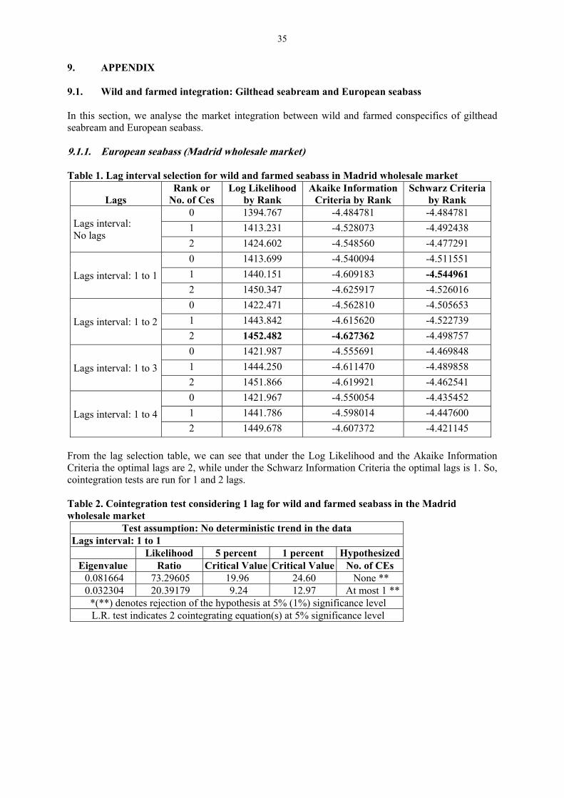
35
9. APPENDIX 9.1. Wild and farmed integration: Gilthead seabream and European seabass In this section, we analyse the market integration between wild and farmed conspecifics of gilthead seabream and European seabass. 9.1.1. European seabass (Madrid wholesale market) Table 1. Lag interval selection for wild and farmed seabass in Madrid wholesale market
Lags Rank or
No. of Ces Log Likelihood
by Rank Akaike Information
Criteria by Rank Schwarz Criteria
by Rank
Lags interval: No lags
0 1394.767 -4.484781 -4.484781
1 1413.231 -4.528073 -4.492438
2 1424.602 -4.548560 -4.477291
Lags interval: 1 to 1
0 1413.699 -4.540094 -4.511551
1 1440.151 -4.609183 -4.544961
2 1450.347 -4.625917 -4.526016
Lags interval: 1 to 2
0 1422.471 -4.562810 -4.505653
1 1443.842 -4.615620 -4.522739
2 1452.482 -4.627362 -4.498757
Lags interval: 1 to 3
0 1421.987 -4.555691 -4.469848
1 1444.250 -4.611470 -4.489858
2 1451.866 -4.619921 -4.462541
Lags interval: 1 to 4
0 1421.967 -4.550054 -4.435452
1 1441.786 -4.598014 -4.447600
2 1449.678 -4.607372 -4.421145
From the lag selection table, we can see that under the Log Likelihood and the Akaike Information Criteria the optimal lags are 2, while under the Schwarz Information Criteria the optimal lags is 1. So, cointegration tests are run for 1 and 2 lags. Table 2. Cointegration test considering 1 lag for wild and farmed seabass in the Madrid wholesale market
Test assumption: No deterministic trend in the data Lags interval: 1 to 1
Likelihood 5 percent 1 percent Hypothesized Eigenvalue Ratio Critical Value Critical Value No. of CEs 0.081664 73.29605 19.96 24.60 None ** 0.032304 20.39179 9.24 12.97 At most 1 **
*(**) denotes rejection of the hypothesis at 5% (1%) significance level L.R. test indicates 2 cointegrating equation(s) at 5% significance level

36
Table 3. Cointegration test considering 2 lags for wild and farmed seabass in the Madrid wholesale market
Test assumption: No deterministic trend in the data Lags interval: 1 to 2
Likelihood 5 percent 1 percent Hypothesized Eigenvalue Ratio Critical Value Critical Value No. of CEs 0.066617 60.02186 19.96 24.60 None ** 0.027485 17.27954 9.24 12.97 At most 1 **
*(**) denotes rejection of the hypothesis at 5% (1%) significance level L.R. test indicates 2 cointegrating equation(s) at 5% significance level
Both cointegration tests, considering 1 and 2 lags, show 2 cointegration equations between wild and farmed seabass in the Madrid wholesale market, consequently, prices are stationary and regression methodology should be used. Table 4. Regression analysis for farmed and wild seabass in the Madrid wholesale market considering 1 lag Dependent Variable: Bass Farmed Method: Least Squares Sample(adjusted): 2 623 Included observations: 622 after adjusting endpoints
Variable Coefficient Std. Error t-Statistic Prob. C 0.113367 0.032829 3.453274 0.0006
Bass Wild -0.013795 0.017448 -0.790627 0.4295 Bass Wild (-1) 0.024946 0.017439 1.430441 0.1531
Bass Farmed (-1) 0.917659 0.015715 58.39355 0.0000 R-squared 0.852848 Mean dependent var 1.778149 Adjusted R-squared 0.852134 S.D. dependent var 0.132282 S.E. of regression 0.050867 Akaike info criterion -3.112791 Sum squared resid 1.599051 Schwarz criterion -3.084283 Log likelihood 972.0780 F-statistic 1193.913 Durbin-Watson stat 2.160663 Prob(F-statistic) 0.000000
Table 5. Regression analysis for wild and farmed seabass in the Madrid wholesale market considering 1 lag Dependent Variable: Bass Wild Method: Least Squares Sample(adjusted): 2 623 Included observations: 622 after adjusting endpoints
Variable Coefficient Std. Error t-Statistic Prob. C 0.258018 0.075666 3.409937 0.0007
Bass Farmed -0.073249 0.092647 -0.790627 0.4295 Bass Farmed (-1) 0.096431 0.092367 1.043994 0.2969
Bass Wild (-1) 0.900062 0.017589 51.17100 0.0000 R-squared 0.816079 Mean dependent var 2.988993 Adjusted R-squared 0.815186 S.D. dependent var 0.272655 S.E. of regression 0.117215 Akaike info criterion -1.443211 Sum squared resid 8.490860 Schwarz criterion -1.414703 Log likelihood 452.8386 F-statistic 914.0446 Durbin-Watson stat 1.522692 Prob(F-statistic) 0.000000
The results from the regression analysis show the lack of integration between wild and farmed seabass in the Madrid wholesale market when considering 1 lag.

37
Table 6. Regression analysis for farmed and wild seabass in the Madrid wholesale market considering 2 lags Dependent Variable: Bass Farmed Method: Least Squares Sample(adjusted): 3 623 Included observations: 621 after adjusting endpoints
Variable Coefficient Std. Error t-Statistic Prob. C 0.111999 0.033478 3.345497 0.0009
Bass Wild -0.021820 0.018044 -1.209223 0.2270 Bass Wild (-1) 0.064863 0.026831 2.417509 0.0159 Bass Wild (-2) -0.037078 0.018006 -2.059242 0.0399
Bass Farmed (-1) 0.838343 0.040128 20.89160 0.0000 Bass Farmed (-2) 0.088822 0.039988 2.221189 0.0267
R-squared 0.854833 Mean dependent var 1.778386 Adjusted R-squared 0.853653 S.D. dependent var 0.132257 S.E. of regression 0.050595 Akaike info criterion -3.120295 Sum squared resid 1.574339 Schwarz criterion -3.077480 Log likelihood 974.8516 F-statistic 724.3008 Durbin-Watson stat 2.016571 Prob(F-statistic) 0.000000
Table 7. Regression analysis for wild and farmed seabass in the Madrid wholesale market considering 2 lags Dependent Variable: Bass Wild Method: Least Squares Sample(adjusted): 3 623 Included observations: 621 after adjusting endpoints
Variable Coefficient Std. Error t-Statistic Prob. C 0.333990 0.074189 4.501912 0.0000
Bass Farmed -0.108708 0.089899 -1.209223 0.2270 Bass Farmed (-1) 0.254772 0.116664 2.183799 0.0294 Bass Farmed (-2) -0.119962 0.089484 -1.340608 0.1805
Bass Wild (-1) 1.137918 0.038925 29.23332 0.0000 Bass Wild (-2) -0.264961 0.038887 -6.813540 0.0000
R-squared 0.829074 Mean dependent var 2.989840 Adjusted R-squared 0.827684 S.D. dependent var 0.272055 S.E. of regression 0.112933 Akaike info criterion -1.514438 Sum squared resid 7.843556 Schwarz criterion -1.471623 Log likelihood 476.2330 F-statistic 596.6079 Durbin-Watson stat 1.968129 Prob(F-statistic) 0.000000
The results from the regression analysis show the potential or limited integration between wild and farmed seabass in the Madrid wholesale market when considering 3 lags.

38
9.1.2. European seabass (Barcelona wholesale market) Table 8. Lag interval selection for wild and farmed seabass in the Barcelona wholesale market
Lags Rank or No. of CE(s)
Log Likelihood by Rank
Akaike Information Criteria by Rank
Schwarz Criteria by Rank
Lags interval: No lags
0 823.3444 -3.526100 -3.526100
1 854.3822 -3.637611 -3.593218
2 864.1426 -3.657998 -3.569212
Lags interval: 1 to 1
0 838.7091 -3.582442 -3.54687
1 864.6355 -3.672255 -3.592217
2 872.6763 -3.685306 -3.560803
Lags interval: 1 to 2
0 866.8185 -3.693843 -3.622582
1 883.3289 -3.743350 -3.627551
2 888.9889 -3.746189 -3.585852
Lags interval: 1 to 3
0 871.2587 -3.703701 -3.596635
1 885.3029 -3.742685 -3.591008
2 890.7209 -3.744486 -3.548199
Lags interval: 1 to 4
0 869.7366 -3.687847 -3.544859
1 883.7652 -3.726848 -3.539175
2 889.4483 -3.729798 -3.497442
From the lag selection table, we can see that under the Akaike and Schwarz Information Criteria the optimal lags are 2, while under the Log Likelihood the optimal lag is 3. So, cointegration tests are run for 2 and 3 lags. Table 9. Cointegration test considering 2 lags for wild and farmed seabass in the Barcelona wholesale market
Test assumption: No deterministic trend in the data Lags interval: 1 to 2
Likelihood 5 percent 1 percent Hypothesized Eigenvalue Ratio Critical Value Critical Value No. of CEs 0.068550 44.34091 19.96 24.60 None ** 0.024050 11.31994 9.24 12.97 At most 1 *
*(**) denotes rejection of the hypothesis at 5% (1%) significance level L.R. test indicates 2 cointegrating equation(s) at 5% significance level
Table 10. Cointegration test considering 3 lags for wild and farmed seabass in the Barcelona wholesale market
Test assumption: No deterministic trend in the data Lags interval: 1 to 3
Likelihood 5 percent 1 percent Hypothesized Eigenvalue Ratio Critical Value Critical Value No. of CEs 0.058739 38.92429 19.96 24.60 None ** 0.023083 10.83602 9.24 12.97 At most 1 *
*(**) denotes rejection of the hypothesis at 5% (1%) significance level L.R. test indicates 2 cointegrating equation(s) at 5% significance level
Both cointegration tests, considering 2 and 3 lags, show 2 cointegration equations between wild and farmed seabass in Barcelona wholesale market, consequently, prices are stationary and regression methodology should be used.

39
Table 11. Regression analysis for farmed and wild seabass in the Barcelona wholesale market considering 2 lags Dependent Variable: Bass Farmed Method: Least Squares Sample(adjusted): 3 468 Included observations: 466 after adjusting endpoints
Variable Coefficient Std. Error t-Statistic Prob. C 0.125806 0.033386 3.768189 0.0002
Bass Wild -0.016475 0.010881 -1.514060 0.1307 Bass Wild (-1) 0.027818 0.013804 2.015249 0.0445 Bass Wild (-2) -0.011695 0.010828 -1.080051 0.2807
Bass Farmed (-1) 0.742875 0.046037 16.13657 0.0000 Bass Farmed (-2) 0.185648 0.045785 4.054755 0.0001
R-squared 0.855275 Mean dependent var 1.736433 Adjusted R-squared 0.853702 S.D. dependent var 0.120596 S.E. of regression 0.046127 Akaike info criterion -3.302056 Sum squared resid 0.978731 Schwarz criterion -3.248698 Log likelihood 775.3791 F-statistic 543.6867 Durbin-Watson stat 2.045046 Prob(F-statistic) 0.000000
Table 12. Regression analysis for wild and farmed seabass in the Barcelona wholesale market considering 2 lags Dependent Variable: Bass Wild Method: Least Squares Sample(adjusted): 3 468 Included observations: 466 after adjusting endpoints
Variable Coefficient Std. Error
t-Statistic Prob.
C 0.357361 0.143928 2.482906 0.0134 Bass Farmed -0.300990 0.198797 -1.514060 0.1307
Bass Farmed (-1) 0.691223 0.244132 2.831350 0.0048 Bass Farmed (-2) -0.204340 0.198940 -1.027145 0.3049
Bass Wild (-1) 0.784168 0.046639 16.81364 0.0000 Bass Wild (-2) -0.012264 0.046338 -0.264658 0.7914
R-squared 0.638990 Mean dependent var 2.978836 Adjusted R-squared 0.635066 S.D. dependent var 0.326372 S.E. of regression 0.197161 Akaike info criterion -0.396805 Sum squared resid 17.88125 Schwarz criterion -0.343446 Log likelihood 98.45550 F-statistic 162.8406 Durbin-Watson stat 1.991624 Prob(F-statistic) 0.000000
The results from the regression analysis show the potential (or limited) integration between wild and farmed seabass in the Barcelona wholesale market when considering 2 lags.

40
Table 13. Regression analysis for farmed and wild seabass in the Barcelona wholesale market considering 3 lags Dependent Variable: Bass Farmed Method: Least Squares Sample(adjusted): 4 468 Included observations: 465 after adjusting endpoints
Variable Coefficient Std. Error t-Statistic Prob. C 0.107546 0.033612 3.199665 0.0015
Bass Wild -0.015598 0.011014 -1.416176 0.1574 Bass Wild (-1) 0.029458 0.013760 2.140816 0.0328 Bass Wild (-2) -0.019376 0.013799 -1.404173 0.1609 Bass Wild (-3) 0.003866 0.010915 0.354166 0.7234
Bass Farmed (-1) 0.713746 0.046531 15.33926 0.0000 Bass Farmed (-2) 0.055961 0.057010 0.981604 0.3268 Bass Farmed (-3) 0.171586 0.046080 3.723636 0.0002
R-squared 0.858646 Mean dependent var 1.736957 Adjusted R-squared 0.856481 S.D. dependent var 0.120194 S.E. of regression 0.045534 Akaike info criterion -3.323648 Sum squared resid 0.947530 Schwarz criterion -3.252387 Log likelihood 780.7482 F-statistic 396.5738 Durbin-Watson stat 1.999482 Prob(F-statistic) 0.000000
Table 14. Regression analysis for wild and farmed seabass in the Barcelona wholesale market considering 3 lags Dependent Variable: Bass Wild Method: Least Squares Sample(adjusted): 4 468 Included observations: 465 after adjusting endpoints
Variable Coefficient Std. Error t-Statistic Prob. C 0.313117 0.143283 2.185311 0.0294
Bass Farmed -0.280128 0.197806 -1.416176 0.1574 Bass Farmed (-1) 0.686618 0.240568 2.854154 0.0045 Bass Farmed (-2) -0.317358 0.241401 -1.314652 0.1893 Bass Farmed (-3) 0.051360 0.198208 0.259120 0.7957
Bass Wild (-1) 0.782626 0.045765 17.10084 0.0000 Bass Wild (-2) -0.161187 0.058117 -2.773509 0.0058 Bass Wild (-3) 0.192120 0.045383 4.233302 0.0000
R-squared 0.651625 Mean dependent var 2.980612 Adjusted R-squared 0.646289 S.D. dependent var 0.324461 S.E. of regression 0.192969 Akaike info criterion -0.435522 Sum squared resid 17.01729 Schwarz criterion -0.364261 Log likelihood 109.2588 F-statistic 122.1148 Durbin-Watson stat 2.025557 Prob(F-statistic) 0.000000
The results from the regression analysis show the potential (or limited) integration between wild and farmed seabass in the Barcelona wholesale market when considering 3 lags.

41
9.1.3. European seabass (French retail) Table 15. Lag interval selection for wild and farmed seabass in the French retail market
Lags Included observations
Rank or No. of Ces
Log Likelihood by Rank
Akaike Information
Criteria by Rank
Schwarz Criteria by
Rank
Lags interval: No lags
74
0 168.4447 -4.55256 -4.55256
1 178.2926 -4.68358 -4.52790
2 183.3416 -4.68491 -4.37355
Lags interval: 1 to 1
55
0 136.6785 -4.82467 -4.67869
1 143.3004 -4.88365 -4.55518
2 146.0930 -4.80338 -4.29242
Lags interval: 1 to 2
38
0 109.2939 -5.33126 -4.98650
1 111.1186 -5.16414 -4.60391
2 112.5361 -4.97559 -4.19989
Lags interval: 1 to 3
28
0 87.80238 -5.414455 -4.843511
1 95.49704 -5.606932 -4.798093
2 97.19978 -5.371413 -4.324681
Lags interval: 1 to 4
22
0 80.45692 -5.85972 -5.066235
1 88.70897 -6.155361 -5.113912
2 89.44081 -5.767346 -4.477933
From the lag selection table, we can see that under the Akaike and Schwarz Information Criteria the optimal lags are 4 (or more), while under the Log Likelihood Criteria the optimal lag is 0. However, the number of observations included in the analysis decreases significantly when the number of lags considered in the model increases. This is because of the existence of gaps in the price series. The cointegration test cannot be run with few observations because the results are not robust. So, cointegration tests are only run for 0 lags. Table 16. Cointegration test considering 0 lags for wild and farmed seabass in the French retail market
Test assumption: No deterministic trend in the data Lags interval: No lags Included observations: 74
Likelihood 5 percent 1 percent Hypothesized Eigenvalue Ratio Critical Value Critical Value No. of CEs 0.233682 29.79371 19.96 24.60 None ** 0.127558 10.09801 9.24 12.97 At most 1 *
*(**) denotes rejection of the hypothesis at 5% (1%) significance level L.R. test indicates 2 cointegrating equation(s) at 5% significance level
The cointegration test, considering no lags, shows 2 cointegration equations between wild and farmed seabass in the French retail market, consequently, prices are stationary and regression methodology should be used.

42
Table 17. Regression analysis for wild and farmed seabass in the Paris wholesale market considering 0 lags Dependent Variable: Bass Farmed Method: Least Squares Sample(adjusted): 4 278 Included observations: 102 Excluded observations: 173 after adjusting endpoints
Variable Coefficient Std. Error t-Statistic Prob. C 2.004472 0.144560 13.86603 0.0000
Bass Wild 0.203525 0.050137 4.059372 0.0001 R-squared 0.141472 Mean dependent var 2.590364 Adjusted R-squared 0.132887 S.D. dependent var 0.088273 S.E. of regression 0.082199 Akaike info criterion -2.139942 Sum squared resid 0.675663 Schwarz criterion -2.088471 Log likelihood 111.1370 F-statistic 16.47850 Durbin-Watson stat 0.911260 Prob(F-statistic) 0.000098
Table 18. Regression analysis for wild and farmed seabass in the Paris wholesale market considering 0 lags Dependent Variable: Bass Wild Method: Least Squares Sample(adjusted): 4 278 Included observations: 102 Excluded observations: 173 after adjusting endpoints
Variable Coefficient Std. Error t-Statistic Prob. C 1.078131 0.443819 2.429212 0.0169
Bass Farmed 0.695112 0.171236 4.059372 0.0001 R-squared 0.141472 Mean dependent var 2.878724 Adjusted R-squared 0.132887 S.D. dependent var 0.163135 S.E. of regression 0.151909 Akaike info criterion -0.911656 Sum squared resid 2.307636 Schwarz criterion -0.860186 Log likelihood 48.49447 F-statistic 16.47850 Durbin-Watson stat 0.363789 Prob(F-statistic) 0.000098
The results from the regression analysis show the integration between wild and farmed seabass in the Paris wholesale market when considering 0 lags. Table 19. Regression analysis for wild and farmed seabass in the Paris wholesale market considering 1 lag Dependent Variable: Bass Farmed Method: Least Squares Sample(adjusted): 5 274 Included observations: 74 Excluded observations: 196 after adjusting endpoints
Variable Coefficient Std. Error t-Statistic Prob. C 0.927575 0.263054 3.526173 0.0007
Bass Wild 0.092037 0.112468 0.818338 0.4159 Bass Wild (-1) 0.031120 0.108013 0.288109 0.7741
Bass Farmed (-1) 0.505015 0.108633 4.648823 0.0000 R-squared 0.368379 Mean dependent var 2.588838 Adjusted R-squared 0.341310 S.D. dependent var 0.086154 S.E. of regression 0.069922 Akaike info criterion -2.430321 Sum squared resid 0.342241 Schwarz criterion -2.305777 Log likelihood 93.92189 F-statistic 13.60868 Durbin-Watson stat 1.785820 Prob(F-statistic) 0.000000

43
Table 20. Regression analysis for wild and farmed seabass in the Paris wholesale market considering 1 lag Dependent Variable: Bass Wild Method: Least Squares Sample(adjusted): 5 274 Included observations: 74 Excluded observations: 196 after adjusting endpoints
Variable Coefficient Std. Error t-Statistic Prob. C 0.346378 0.299077 1.158155 0.2507
Bass Farmed 0.102961 0.125817 0.818338 0.4159 Bass Farmed (-1) -0.023846 0.131414 -0.181456 0.8565
Bass Wild (-1) 0.806641 0.061414 13.13443 0.0000 R-squared 0.767941 Mean dependent var 2.857838 Adjusted R-squared 0.757995 S.D. dependent var 0.150335 S.E. of regression 0.073956 Akaike info criterion -2.318161 Sum squared resid 0.382862 Schwarz criterion -2.193617 Log likelihood 89.77196 F-statistic 77.21559 Durbin-Watson stat 2.185101 Prob(F-statistic) 0.000000
The results from the regression analysis show the lack of integration between wild and farmed seabass in the Paris wholesale market when considering 1 lag. 9.1.4. Gilthead seabream (Madrid wholesale market) Table 21. Lag interval selection for wild and farmed seabream in the Madrid wholesale market
Lags Rank or
No. of Ces Log Likelihood
by Rank Akaike Information
Criteria by Rank Schwarz Criteria
by Rank
Lags interval: No lags
0 1773.149 -6.846134 -6.846134
1 1783.263 -6.865879 -6.824856
2 1784.296 -6.850564 -6.768518
Lags interval: 1 to 1
0 1700.650 -6.841332 -6.807408
1 1711.851 -6.866335 -6.790006
2 1712.716 -6.84966 -6.730926
Lags interval: 1 to 2
0 1624.991 -6.794082 -6.724075
1 1635.792 -6.818454 -6.704692
2 1636.208 -6.799193 -6.641678
Lags interval: 1 to 3
0 1558.401 -6.782463 -6.673976
1 1570.021 -6.811498 -6.657808
2 1570.609 -6.792144 -6.593252
Lags interval: 1 to 4
0 1500.959 -6.811737 -6.662099
1 1511.731 -6.838214 -6.641814
2 1512.154 -6.817222 -6.574060
From the lag selection table, we can see that under the Log Likelihood and the Schwarz Information Criteria the optimal is no lags, while under the Akaike Information Criteria the optimal lags is 1. So, cointegration tests are run for 0 and 1 lag.

44
Table 22. Cointegration test considering no lags for wild and farmed seabream in the Madrid wholesale market
Test assumption: No deterministic trend in the data Lags interval: No lags
Likelihood 5 percent 1 percent Hypothesized Eigenvalue Ratio Critical Value Critical Value No. of CEs 0.038297 22.29477 19.96 24.60 None * 0.003983 2.067092 9.24 12.97 At most 1
*(**) denotes rejection of the hypothesis at 5% (1%) significance level L.R. test indicates 1 cointegrating equation(s) at 5% significance level
Table 23. Cointegration test considering 1 lag for wild and farmed seabream in the Madrid wholesale market
Test assumption: No deterministic trend in the data Lags interval: 1 to 1
Likelihood 5 percent 1 percent Hypothesized Eigenvalue Ratio Critical Value Critical Value No. of CEs 0.044160 24.13078 19.96 24.60 None * 0.003480 1.729244 9.24 12.97 At most 1
*(**) denotes rejection of the hypothesis at 5% (1%) significance level L.R. test indicates 1 cointegrating equation(s) at 5% significance level
Both cointegration tests, considering no lags and 1 lag, show 1 cointegration equation between wild and farmed seabream in the Madrid wholesale market. So the stationarity behavior of the series is analysed. Table 24. Unit root test considering intercept and no lags and 1 lag for wild and farmed seabream in Madrid wholesale market Series Lags ADF Test
Statistic Critical Values
Farmed seabream 0 -3.724575 1%: -3.4453 5%: -2.8674 10%: -2.5699 Wild seabream 0 -2.049078 1%: -3.4433 5%: -2.8665 10%: -2.5694 Farmed seabream 1 -3.630154 1%: -3.4458 5%: -2.8677 10%: -2.5700 Wild seabream 1 -2.492221 1%: -3.4433 5%: -2.8665 10%: -2.5694
The ADF Test statistics for wild seabream (-2.049 and -2.492) are higher than the MacKinnon critical value for rejection of the hypothesis of a unit root at a 5% significance level (-2.866). So, the wild seabream price series behaves as a non-stationary series. While the farmed seabream price series behaves as stationary. Therefore, there is no market integration between wild and farmed seabream in the Madrid wholesale market.

45
9.1.5. Gilthead seabream (Barcelona wholesale market) Table 25. Lag interval selection for wild and farmed seabream in the Barcelona wholesale market
Lags Rank or
No. of Ces Log Likelihood
by Rank Akaike Information
Criteria by Rank Schwarz Criteria
by Rank
Lags interval: No lags
0 952.8161 -4.080583 -4.080583
1 987.1482 -4.206202 -4.161809
2 991.9419 -4.205319 -4.116532
Lags interval: 1 to 1
0 959.9336 -4.102719 -4.067147
1 995.7863 -4.235134 -4.155096
2 999.4217 -4.229278 -4.104774
Lags interval: 1 to 2
0 963.6102 -4.110151 -4.038891
1 997.2240 -4.233222 -4.117423
2 1000.4150 -4.22544 -4.065103
Lags interval: 1 to 3
0 965.6643 -4.110622 -4.003556
1 997.5639 -4.226569 -4.074892
2 1001.1850 -4.220624 -4.024337
Lags interval: 1 to 4
0 976.7978 -4.150315 -4.007326
1 1001.1310 -4.233829 -4.046157
2 1005.6470 -4.231735 -3.999379
Lags interval: 1 to 5
0 979.5822 -4.154035 -3.975007
1 1001.4300 -4.226968 -4.003182
2 1006.7340 -4.228284 -3.959741
Lags interval: 1 to 6
0 978.8902 -4.142691 -3.927503
1 998.6663 -4.206795 -3.946777
2 1004.1440 -4.208868 -3.904019
From the lag selection table, we can see that under the Akaike Information Criteria the optimal lags is 1, under the Schwarz Information Criteria the optimal lags is 0, while under the Log Likelihood the optimal lag is 5. So, cointegration tests are run for 0, 1 and 5 lags. Table 26. Cointegration test considering no lags for wild and farmed seabream in the Barcelona wholesale market
Test assumption: No deterministic trend in the data Lags interval: No lags
Likelihood 5 percent 1 percent Hypothesized Eigenvalue Ratio Critical Value Critical Value No. of CEs 0.136734 78.25155 19.96 24.60 None ** 0.020321 9.587526 9.24 12.97 At most 1 *
*(**) denotes rejection of the hypothesis at 5% (1%) significance level L.R. test indicates 2 cointegrating equation(s) at 5% significance level
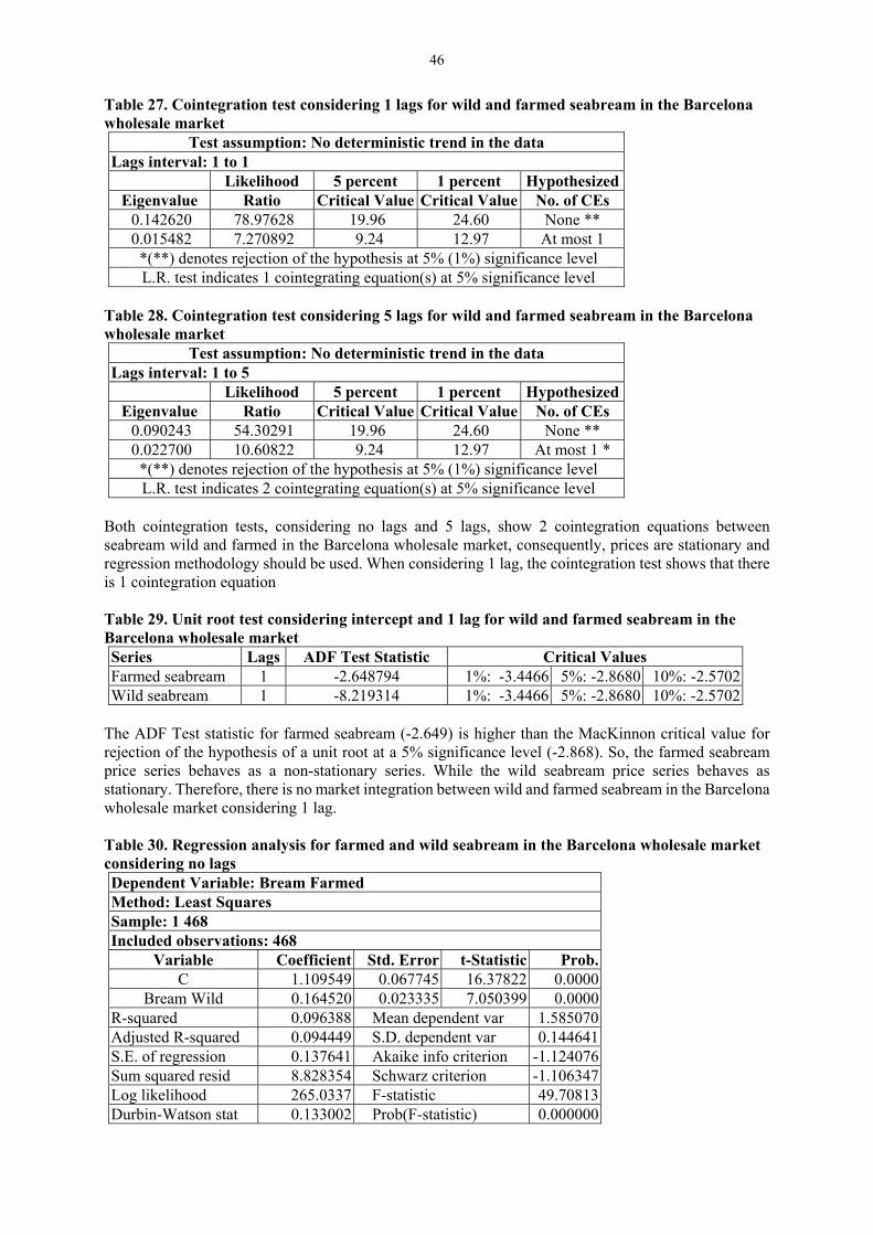
46
Table 27. Cointegration test considering 1 lags for wild and farmed seabream in the Barcelona wholesale market
Test assumption: No deterministic trend in the data Lags interval: 1 to 1
Likelihood 5 percent 1 percent Hypothesized Eigenvalue Ratio Critical Value Critical Value No. of CEs 0.142620 78.97628 19.96 24.60 None ** 0.015482 7.270892 9.24 12.97 At most 1
*(**) denotes rejection of the hypothesis at 5% (1%) significance level L.R. test indicates 1 cointegrating equation(s) at 5% significance level
Table 28. Cointegration test considering 5 lags for wild and farmed seabream in the Barcelona wholesale market
Test assumption: No deterministic trend in the data Lags interval: 1 to 5
Likelihood 5 percent 1 percent Hypothesized Eigenvalue Ratio Critical Value Critical Value No. of CEs 0.090243 54.30291 19.96 24.60 None ** 0.022700 10.60822 9.24 12.97 At most 1 *
*(**) denotes rejection of the hypothesis at 5% (1%) significance level L.R. test indicates 2 cointegrating equation(s) at 5% significance level
Both cointegration tests, considering no lags and 5 lags, show 2 cointegration equations between seabream wild and farmed in the Barcelona wholesale market, consequently, prices are stationary and regression methodology should be used. When considering 1 lag, the cointegration test shows that there is 1 cointegration equation Table 29. Unit root test considering intercept and 1 lag for wild and farmed seabream in the Barcelona wholesale market Series Lags ADF Test Statistic Critical Values Farmed seabream 1 -2.648794 1%: -3.4466 5%: -2.8680 10%: -2.5702 Wild seabream 1 -8.219314 1%: -3.4466 5%: -2.8680 10%: -2.5702
The ADF Test statistic for farmed seabream (-2.649) is higher than the MacKinnon critical value for rejection of the hypothesis of a unit root at a 5% significance level (-2.868). So, the farmed seabream price series behaves as a non-stationary series. While the wild seabream price series behaves as stationary. Therefore, there is no market integration between wild and farmed seabream in the Barcelona wholesale market considering 1 lag. Table 30. Regression analysis for farmed and wild seabream in the Barcelona wholesale market considering no lags Dependent Variable: Bream Farmed Method: Least Squares Sample: 1 468 Included observations: 468
Variable Coefficient Std. Error t-Statistic Prob. C 1.109549 0.067745 16.37822 0.0000
Bream Wild 0.164520 0.023335 7.050399 0.0000 R-squared 0.096388 Mean dependent var 1.585070 Adjusted R-squared 0.094449 S.D. dependent var 0.144641 S.E. of regression 0.137641 Akaike info criterion -1.124076 Sum squared resid 8.828354 Schwarz criterion -1.106347 Log likelihood 265.0337 F-statistic 49.70813 Durbin-Watson stat 0.133002 Prob(F-statistic) 0.000000

47
Table 31. Regression analysis for wild and farmed seabream in the Barcelona wholesale market considering no lags Dependent Variable: Bream Wild Method: Least Squares Sample: 1 468 Included observations: 468
Variable Coefficient Std. Error t-Statistic Prob. C 1.961699 0.132262 14.83189 0.0000
Bream Farmed 0.585874 0.083098 7.050399 0.0000 R-squared 0.096388 Mean dependent var 2.890350 Adjusted R-squared 0.094449 S.D. dependent var 0.272950 S.E. of regression 0.259740 Akaike info criterion 0.145996 Sum squared resid 31.43872 Schwarz criterion 0.163725 Log likelihood -32.16310 F-statistic 49.70813 Durbin-Watson stat 0.539303 Prob(F-statistic) 0.000000
The results from the regression analysis show the presence of integration between wild and farmed seabream in the Barcelona wholesale market when considering 0 lags. Table 32. Regression analysis for wild and farmed seabream in the Barcelona wholesale market considering 5 lags Dependent Variable: Bream Wild Method: Least Squares Sample(adjusted): 6 468 Included observations: 463 after adjusting endpoints
Variable Coefficient Std. Error t-Statistic Prob. C 0.621727 0.123824 5.021074 0.0000
Bream Farmed 0.166352 0.212712 0.782052 0.4346 Bream Farmed (-1) 0.095465 0.267441 0.356957 0.7213 Bream Farmed (-2) -0.084711 0.270021 -0.313719 0.7539 Bream Farmed (-3) 0.334772 0.269798 1.240824 0.2153 Bream Farmed (-4) -0.137733 0.266700 -0.516434 0.6058 Bream Farmed (-5) -0.226313 0.211441 -1.070337 0.2850
Bream Wild (-1) 0.789667 0.047007 16.79907 0.0000 Bream Wild (-2) -0.040080 0.059734 -0.670983 0.5026 Bream Wild (-3) -0.011846 0.059617 -0.198700 0.8426 Bream Wild (-4) -0.102820 0.059200 -1.736828 0.0831 Bream Wild (-5) 0.069032 0.046908 1.471639 0.1418
R-squared 0.592121 Mean dependent var 2.892563 Adjusted R-squared 0.582173 S.D. dependent var 0.272118 S.E. of regression 0.175896 Akaike info criterion -0.612270 Sum squared resid 13.95369 Schwarz criterion -0.505029 Log likelihood 153.7406 F-statistic 59.52010 Durbin-Watson stat 2.000442 Prob(F-statistic) 0.000000

48
Table 33. Regression analysis for farmed and wild seabream in the Barcelona wholesale market considering 5 lags Dependent Variable: Bream Farmed Method: Least Squares Sample(adjusted): 6 468 Included observations: 463 after adjusting endpoints
Variable Coefficient Std. Error t-Statistic Prob. C 0.043442 0.028073 1.547473 0.1225
Bream Wild 0.008141 0.010410 0.782052 0.4346 Bream Wild (-1) -0.006985 0.013255 -0.526956 0.5985 Bream Wild (-2) 0.004067 0.013220 0.307668 0.7585 Bream Wild (-3) 0.008734 0.013183 0.662526 0.5080 Bream Wild (-4) 0.008161 0.013134 0.621313 0.5347 Bream Wild (-5) -0.013617 0.010382 -1.311537 0.1903
Bream Farmed (-1) 0.775694 0.046553 16.66266 0.0000 Bream Farmed (-2) 0.180237 0.059135 3.047899 0.0024 Bream Farmed (-3) 0.109156 0.059565 1.832541 0.0675 Bream Farmed (-4) 0.028451 0.059002 0.482204 0.6299 Bream Farmed (-5) -0.136285 0.046393 -2.937638 0.0035
R-squared 0.929481 Mean dependent var 1.586418 Adjusted R-squared 0.927761 S.D. dependent var 0.144776 S.E. of regression 0.038912 Akaike info criterion -3.629459 Sum squared resid 0.682874 Schwarz criterion -3.522218 Log likelihood 852.2198 F-statistic 540.4063 Durbin-Watson stat 2.037963 Prob(F-statistic) 0.000000
The results from the regression analysis show the lack of integration between wild and farmed seabream in the Barcelona wholesale market when considering 5 lags. 9.2. Wild and farmed integration: Other species In this section, we analyse the market integration between wild and farmed conspecifics of species other than seabream and seabass.

49
9.2.1. Turbot (Scophthalmus maximus) (Madrid wholesale market) Table 34. Lag interval selection for wild and farmed turbot in the Madrid wholesale market
Lags Rank or No. of Ces
Log Likelihood by Rank
Akaike Information Criteria by Rank
Schwarz Criteria by Rank
Lags interval: No lags
0 2117.713 -6.809368 -6.809368
1 2132.299 -6.840189 -6.804554
2 2137.272 -6.840102 -6.768833
Lags interval: 1 to 1
0 2126.261 -6.834979 -6.806435
1 2144.122 -6.876400 -6.812177
2 2149.937 -6.879024 -6.779123
Lags interval: 1 to 2
0 2124.908 -6.828736 -6.771578
1 2142.786 -6.870277 -6.777396
2 2149.206 -6.874859 -6.746255
Lags interval: 1 to 3
0 2142.476 -6.883606 -6.797762
1 2156.505 -6.912777 -6.791165
2 2163.117 -6.917986 -6.760606
Lags interval: 1 to 4
0 2141.242 -6.877804 -6.763203
1 2154.501 -6.904535 -6.754121
2 2162.481 -6.914180 -6.727952
From the lag selection table, we can see that under the Log Likelihood and the Akaike Information Criteria the optimal lags are 3 lags and 1 lag under the Schwarz Information Criteria. So, cointegration tests are run for 1 and 3 lags. Table 35. Cointegration test considering 1 lags for wild and farmed turbot in the Madrid wholesale market
Test assumption: No deterministic trend in the data Lags interval: 1 to 1
Likelihood 5 percent 1 percent Hypothesized Eigenvalue Ratio Critical Value Critical Value No. of CEs 0.055901 47.35251 19.96 24.60 None ** 0.018554 11.63008 9.24 12.97 At most 1 *
*(**) denotes rejection of the hypothesis at 5% (1%) significance level L.R. test indicates 2 cointegrating equation(s) at 5% significance level
Table 36. Cointegration test considering 3 lags for wild and farmed turbot in the Madrid wholesale market
Test assumption: No deterministic trend in the data Lags interval: 1 to 3
Likelihood 5 percent 1 percent Hypothesized Eigenvalue Ratio Critical Value Critical Value No. of CEs 0.044314 41.28150 19.96 24.60 None ** 0.021138 13.22458 9.24 12.97 At most 1 **
*(**) denotes rejection of the hypothesis at 5% (1%) significance level L.R. test indicates 2 cointegrating equation(s) at 5% significance level
The cointegration test, considering 1 and 3 lags, shows 2 cointegration equations between wild and farmed turbot in Madrid wholesale market. Therefore, prices are stationary and regression methodology should be used.

50
Table 37. Regression considering 3 lags for farmed and wild turbot in the Madrid wholesale market Dependent Variable: Turbot farmed Madrid Method: Least Squares Sample(adjusted): 4 623 Included observations: 620 after adjusting endpoints
Variable Coefficient Std. Error t-Statistic Prob. C 0.083066 0.024163 3.437689 0.0006
Turbot farmed Madrid (-1) 1.125581 0.040279 27.94474 0.0000 Turbot farmed Madrid (-2) -0.113931 0.063231 -1.801833 0.0721 Turbot farmed Madrid (-3) -0.038059 0.045636 -0.833968 0.4046
Turbot wild Madrid 0.008451 0.019989 0.422773 0.6726 Turbot wild Madrid (-1) -0.023344 0.029341 -0.795607 0.4266 Turbot wild Madrid (-2) 0.032841 0.029340 1.119329 0.2634 Turbot wild Madrid (-3) -0.026144 0.019745 -1.324103 0.1860
R-squared 0.952517 Mean dependent var 2.181020 Adjusted R-squared 0.951974 S.D. dependent var 0.138100 S.E. of regression 0.030264 Akaike info criterion -4.144866 Sum squared resid 0.560554 Schwarz criterion -4.087708 Log likelihood 1292.908 F-statistic 1753.817 Durbin-Watson stat 2.004249 Prob(F-statistic) 0.000000
Table 38. Regression considering 3 lags for wild and farmed turbot in the Madrid wholesale market Dependent Variable: Turbot wild Madrid Method: Least Squares Sample(adjusted): 4 623 Included observations: 620 after adjusting endpoints
Variable Coefficient Std. Error t-Statistic Prob. C 0.110714 0.049123 2.253797 0.0246
Turbot farmed Madrid 0.034549 0.081721 0.422773 0.6726 Turbot farmed Madrid (-1) -0.012055 0.122865 -0.098119 0.9219 Turbot farmed Madrid (-2) 0.073429 0.128154 0.572972 0.5669 Turbot farmed Madrid (-3) -0.027418 0.092320 -0.296985 0.7666
Turbot wild Madrid (-1) 1.076284 0.040379 26.65465 0.0000 Turbot wild Madrid (-2) -0.136410 0.059129 -2.307012 0.0214 Turbot wild Madrid (-3) -0.022892 0.039969 -0.572735 0.5670
R-squared 0.901127 Mean dependent var 3.124293 Adjusted R-squared 0.899996 S.D. dependent var 0.193506 S.E. of regression 0.061193 Akaike info criterion -2.736737 Sum squared resid 2.291711 Schwarz criterion -2.679580 Log likelihood 856.3886 F-statistic 796.8207 Durbin-Watson stat 1.923573 Prob(F-statistic) 0.000000
The results from the regression analysis show the lack of integration between wild and farmed turbot in the Madrid wholesale market when considering 3 lags.

51
Table 39. Regression considering 2 lags for wild and farmed turbot in the Madrid wholesale market Dependent Variable: Turbot wild Madrid Method: Least Squares Sample(adjusted): 3 623 Included observations: 621 after adjusting endpoints
Variable Coefficient Std. Error t-Statistic Prob. C 0.103335 0.048377 2.136022 0.0331
Turbot wild Madrid (-1) 1.082801 0.039705 27.27145 0.0000 Turbot wild Madrid (-2) -0.163416 0.039324 -4.155643 0.0000 Turbot farmed Madrid 0.044728 0.081276 0.550322 0.5823
Turbot farmed Madrid (-1) -0.020657 0.122298 -0.168906 0.8659 Turbot farmed Madrid (-2) 0.044336 0.082389 0.538130 0.5907 R-squared 0.901550 Mean dependent var 3.123630 Adjusted R-squared 0.900749 S.D. dependent var 0.194056 S.E. of regression 0.061136 Akaike info criterion -2.741831 Sum squared resid 2.298598 Schwarz criterion -2.699016 Log likelihood 857.3385 F-statistic 1126.363 Durbin-Watson stat 2.010463 Prob(F-statistic) 0.000000
Table 40. Regression considering 2 lags for farmed and wild turbot in the Madrid wholesale market Dependent Variable: Turbot farmed Madrid Method: Least Squares Sample(adjusted): 3 623 Included observations: 621 after adjusting endpoints
Variable Coefficient Std. Error t-Statistic Prob. C 0.075831 0.023890 3.174190 0.0016
Turbot wild Madrid 0.011004 0.019996 0.550322 0.5823 Turbot wild Madrid (-1) -0.020000 0.029262 -0.683476 0.4946 Turbot wild Madrid (-2) 0.002926 0.019777 0.147934 0.8824
Turbot farmed Madrid (-1) 1.129508 0.040069 28.18900 0.0000 Turbot farmed Madrid (-2) -0.155667 0.040391 -3.853990 0.0001 R-squared 0.952099 Mean dependent var 2.181070 Adjusted R-squared 0.951710 S.D. dependent var 0.137994 S.E. of regression 0.030324 Akaike info criterion -4.144127 Sum squared resid 0.565527 Schwarz criterion -4.101312 Log likelihood 1292.751 F-statistic 2444.811 Durbin-Watson stat 2.003391 Prob(F-statistic) 0.000000
The results from the regression analysis show the lack of integration between wild and farmed turbot in the Madrid wholesale market when considering 2 lags.

52
9.2.2. Sole (Solea spp.) (Madrid wholesale market) Table 41. Lag interval selection for wild and farmed sole in the Madrid wholesale market
Lags Rank or No. of Ces
Log Likelihood by Rank
Akaike Information Criteria by Rank
Schwarz Criteria by Rank
Lags interval: No lags
0 571.4617 -8.163738 -8.163738
1 574.0108 -8.128726 -8.023668
2 575.2968 -8.075669 -7.865552
Lags interval: 1 to 1
0 571.2381 -8.161699 -8.077253
1 574.6160 -8.138360 -7.948358
2 576.2593 -8.090062 -7.794504
Lags interval: 1 to 2
0 574.5791 -8.211292 -8.041596
1 577.8710 -8.186536 -7.910780
2 578.9017 -8.129010 -7.747194
Lags interval: 1 to 3
0 570.0202 -8.146280 -7.890515
1 573.4847 -8.123865 -7.761531
2 574.7470 -8.069299 -7.600397
Lags interval: 1 to 4
0 572.7825 -8.187979 -7.845313
1 576.2887 -8.166010 -7.716262
2 578.5713 -8.126048 -7.569217
From the lag selection table, we can see that under the Log Likelihood and the Akaike Information Criteria the optimal lags are 2 lags, while under the Schwarz Information Criteria the optimal lags are no lags, consequently, cointegration tests are run only for 0 and 2 lags. Table 42. Cointegration test considering no lags for wild and farmed sole in the Madrid wholesale market
Test assumption: No deterministic trend in the data Lags interval: No lags
Likelihood 5 percent 1 percent Hypothesized Eigenvalue Ratio Critical Value Critical Value No. of CEs 0.035762 7.670350 19.96 24.60 None 0.018204 2.572004 9.24 12.97 At most 1
*(**) denotes rejection of the hypothesis at 5% (1%) significance level L.R. rejects any cointegration at 5% significance level
Table 43. Cointegration test considering 2 lags for wild and farmed sole in the Madrid wholesale market
Test assumption: No deterministic trend in the data Lags interval: 1 to 2
Likelihood 5 percent 1 percent Hypothesized Eigenvalue Ratio Critical Value Critical Value No. of CEs 0.046588 8.645063 19.96 24.60 None 0.014826 2.061366 9.24 12.97 At most 1
*(**) denotes rejection of the hypothesis at 5% (1%) significance level L.R. rejects any cointegration at 5% significance level
The cointegration test, considering 0 and 2 lags, show 0 cointegration equations between wild and farmed turbot in the Madrid wholesale market. Therefore, there is no market integration between wild and farmed sole in the Madrid wholesale market.

53
9.2.3. Turbot (Scophthalmus maximus) (Barcelona wholesale market) Table 44. Lag interval selection for wild and farmed turbot in the Barcelona wholesale market
Lags Rank or No. of Ces
Log Likelihood by Rank
Akaike Information Criteria by Rank
Schwarz Criteria by Rank
Lags interval: No lags
0 941.6926 -4.032945 -4.032945
1 980.8899 -4.179400 -4.135007
2 983.5505 -4.169381 -4.080595
Lags interval: 1 to 1
0 945.2929 -4.039884 -4.004311
1 979.0243 -4.163195 -4.083157
2 981.7117 -4.153269 -4.028766
Lags interval: 1 to 2
0 950.6946 -4.054600 -3.983340
1 978.2768 -4.151728 -4.035929
2 980.7318 -4.140782 -3.980445
Lags interval: 1 to 3
0 955.0115 -4.064705 -3.957639
1 978.2162 -4.143173 -3.991497
2 980.4546 -4.131270 -3.934982
Lags interval: 1 to 4
0 955.3436 -4.057640 -3.914651
1 976.9710 -4.129464 -3.941792
2 979.0335 -4.116775 -3.884419
From the lag selection table, we can see that under the Log Likelihood, the Akaike and Schwarz Information Criteria the optimal lags are no lags, consequently, cointegration tests are run only for no lags. Table 45. Cointegration test considering no lags for wild and farmed turbot in the Barcelona wholesale market
Test assumption: No deterministic trend in the data Lags interval: No lags
Likelihood 5 percent 1 percent Hypothesized Eigenvalue Ratio Critical Value Critical Value No. of CEs 0.154535 83.71565 19.96 24.60 None ** 0.011329 5.321044 9.24 12.97 At most 1
*(**) denotes rejection of the hypothesis at 5% (1%) significance level L.R. test indicates 1 cointegrating equation(s) at 5% significance level
The cointegration test, considering no lags, shows 1 cointegration equation between wild and farmed turbot in Barcelona wholesale market. So the stationarity behavior of the series is analysed. Table 46. Unit root test considering intercept and no lags for wild and farmed turbot in the Barcelona wholesale market Series Lags ADF Test
Statistic Critical Values
Farmed turbot 0 -2.272751 1%: -3.4466 5%: -2.8680 10%: -2.5702 Wild turbot 0 -8.619563 1%: -3.4466 5%: -2.8680 10%: -2.5702
The ADF Test statistic for farmed turbot is higher than for the MacKinnon critical value for rejection of the hypothesis of a unit root at a 5% significance level. So, the farmed turbot price series behaves as a non-stationary series. While the wild turbot price series behaves as stationary. Therefore, there is no market integration between wild and farmed turbot in the Barcelona wholesale market.

54
9.2.4. Blackspot (red) seabream (Pagellus bogaraveo) (Barcelona wholesale market) Table 47. Lag interval selection for wild and farmed blackspot seabream in the Barcelona wholesale market
Lags Rank or No. of Ces
Log Likelihood by Rank
Akaike Information Criteria by Rank
Schwarz Criteria by Rank
Lags interval: No lags
0 128.1625 -0.985866 -0.985866
1 146.0919 -1.085323 -1.016848
2 156.3623 -1.125864 -0.988914
Lags interval: 1 to 1
0 101.2478 -0.88007 -0.818565
1 119.6521 -1.001376 -0.86299
2 127.5447 -1.027554 -0.812286
Lags interval: 1 to 2
0 92.75395 -0.882854 -0.747125
1 109.9868 -1.010279 -0.789719
2 115.7323 -1.018044 -0.712654
Lags interval: 1 to 3
0 82.54147 -0.844808 -0.620761
1 106.7777 -1.075182 -0.757782
2 110.8441 -1.064001 -0.653248
Lags interval: 1 to 4
0 85.97225 -0.952003 -0.626514
1 101.4360 -1.094367 -0.667163
2 103.972 -1.060844 -0.531924
From the lag selection table, we can see that under the Log Likelihood, the Akaike and Schwarz Information Criteria the optimal lags are no lags, consequently, cointegration tests are run only for no lags. Table 48. Cointegration test considering no lags for wild and farmed blackspot seabream in the Barcelona wholesale market
Test assumption: No deterministic trend in the data Lags interval: No lags
Likelihood 5 percent 1 percent Hypothesized Eigenvalue Ratio Critical Value Critical Value No. of CEs 0.128830 56.39953 19.96 24.60 None ** 0.075962 20.54067 9.24 12.97 At most 1 **
*(**) denotes rejection of the hypothesis at 5% (1%) significance level L.R. test indicates 2 cointegrating equation(s) at 5% significance level
The cointegration test considering no lags, shows 2 cointegration equations between blackspot seabream wild and farmed in Barcelona wholesale market, consequently, prices are stationary and regression methodology should be used.

55
Table 49. Regression considering 1 lag for farmed and wild blackspot seabream in the Barcelona wholesale market Dependent Variable: Blackspot seabream farmed Method: Least Squares Sample(adjusted): 2 462 Included observations: 260 Excluded observations: 201 after adjusting endpoints
Variable Coefficient Std. Error t-Statistic Prob. C -0.118046 0.186558 -0.632758 0.5275
Blackspot seabream farmed (-1) 0.881265 0.028292 31.14905 0.0000 Blackspot seabream wild 0.153931 0.071492 2.153129 0.0322
Blackspot seabream wild (-1) -0.036651 0.076784 -0.477322 0.6335 R-squared 0.792277 Mean dependent var 1.943651 Adjusted R-squared 0.789843 S.D. dependent var 0.421168 S.E. of regression 0.193075 Akaike info criterion -0.436207 Sum squared resid 9.543192 Schwarz criterion -0.381428 Log likelihood 60.70695 F-statistic 325.4708 Durbin-Watson stat 2.421581 Prob(F-statistic) 0.000000
Table 50. Regression considering 1 lag for wild and farmed blackspot seabream in the Barcelona wholesale market Dependent Variable: Blackspot seabream wild Method: Least Squares Sample(adjusted): 2 462 Included observations: 260 Excluded observations: 201 after adjusting endpoints
Variable Coefficient Std. Error t-Statistic Prob. C 0.919224 0.151217 6.078825 0.0000
Blackspot seabream farmed 0.115552 0.053667 2.153129 0.0322 Blackspot seabream farmed (-1) -0.140834 0.052922 -2.661183 0.0083
Blackspot seabream wild (-1) 0.699739 0.050171 13.94713 0.0000 R-squared 0.446349 Mean dependent var 2.892864 Adjusted R-squared 0.439861 S.D. dependent var 0.223514 S.E. of regression 0.167284 Akaike info criterion -0.722988 Sum squared resid 7.163847 Schwarz criterion -0.668208 Log likelihood 97.98847 F-statistic 68.79512 Durbin-Watson stat 1.771851 Prob(F-statistic) 0.000000
The results from the regression analysis show the integration between wild and farmed blackspot seabream in the Barcelona wholesale market when considering 1 lag.

56
Table 51. Regression considering 5 lags for wild and farmed blackspot seabream in the Barcelona wholesale market Dependent Variable: Blackspot seabream wild Method: Least Squares Sample(adjusted): 55 412 Included observations: 147 Excluded observations: 211 after adjusting endpoints
Variable Coefficient Std. Error t-Statistic Prob. C 1.623646 0.302727 5.363398 0.0000
Blackspot seabream farmed 0.165703 0.066761 2.482043 0.0143 Blackspot seabream farmed (-1) -0.220419 0.084205 -2.617666 0.0099 Blackspot seabream farmed (-2) 0.155832 0.088490 1.761006 0.0805 Blackspot seabream farmed (-3) -0.069374 0.089288 -0.776963 0.4385 Blackspot seabream farmed (-4) -0.054242 0.086766 -0.625157 0.5329 Blackspot seabream farmed (-5) -0.022267 0.067387 -0.330433 0.7416
Blackspot seabream wild (-1) 0.772977 0.085571 9.033116 0.0000 Blackspot seabream wild (-2) -0.169049 0.101957 -1.658049 0.0996 Blackspot seabream wild (-3) 0.029991 0.102485 0.292643 0.7702 Blackspot seabream wild (-4) -0.118069 0.100221 -1.178079 0.2408 Blackspot seabream wild (-5) -0.053471 0.092120 -0.580444 0.5626
R-squared 0.521328 Mean dependent var 2.867458 Adjusted R-squared 0.482325 S.D. dependent var 0.217011 S.E. of regression 0.156139 Akaike info criterion -0.798033 Sum squared resid 3.291217 Schwarz criterion -0.553916 Log likelihood 70.65542 F-statistic 13.36638 Durbin-Watson stat 1.995746 Prob(F-statistic) 0.000000
Table 52. Regression considering 5 lags for wild and farmed blackspot seabream in the Barcelona wholesale market Dependent Variable: Blackspot seabream farmed Method: Least Squares Sample(adjusted): 55 412 Included observations: 147 Excluded observations: 211 after adjusting endpoints
Variable Coefficient Std. Error t-Statistic Prob. C -0.039830 0.420344 -0.094757 0.9246
Blackspot seabream wild 0.263376 0.106113 2.482043 0.0143 Blackspot seabream wild (-1) -0.153432 0.136011 -1.128082 0.2613 Blackspot seabream wild (-2) 0.004411 0.129842 0.033972 0.9729 Blackspot seabream wild (-3) -0.176283 0.128353 -1.373424 0.1719 Blackspot seabream wild (-4) 0.202698 0.125796 1.611319 0.1094 Blackspot seabream wild (-5) -0.071590 0.116120 -0.616512 0.5386
Blackspot seabream farmed (-1) 0.819221 0.082889 9.883339 0.0000 Blackspot seabream farmed (-2) 0.022262 0.112821 0.197324 0.8439 Blackspot seabream farmed (-3) -0.041035 0.112765 -0.363902 0.7165 Blackspot seabream farmed (-4) 0.182321 0.108417 1.681661 0.0949 Blackspot seabream farmed (-5) -0.070729 0.084774 -0.834324 0.4056
R-squared 0.794633 Mean dependent var 1.891964 Adjusted R-squared 0.777899 S.D. dependent var 0.417695 S.E. of regression 0.196850 Akaike info criterion -0.334645 Sum squared resid 5.231226 Schwarz criterion -0.090528 Log likelihood 36.59638 F-statistic 47.48718 Durbin-Watson stat 2.146539 Prob(F-statistic) 0.000000

57
The results from the regression analysis show the integration between wild and farmed blackspot seabream in the Barcelona wholesale market when considering 5 lags. 9.2.5. Atlantic cod (Gadus morhua) (Barcelona wholesale market) Table 53. Lag interval selection for wild and farmed cod in the Barcelona wholesale market
Lags Rank or No. of Ces
Log Likelihood by Rank
Akaike Information Criteria by Rank
Schwarz Criteria by Rank
Lags interval: No lags
0 471.1776 -2.127213 -2.127213
1 530.1068 -2.370685 -2.324482
2 561.1630 -2.488321 -2.395915
Lags interval: 1 to 1
0 518.2373 -2.369757 -2.332218
1 553.8724 -2.510933 -2.426469
2 574.7387 -2.584049 -2.452661
Lags interval: 1 to 2
0 539.4415 -2.483371 -2.407500
1 561.3505 -2.562385 -2.439094
2 575.7537 -2.606326 -2.435615
Lags interval: 1 to 3
0 545.8391 -2.530043 -2.415019
1 560.8047 -2.577273 -2.414323
2 572.3742 -2.608409 -2.397531
Lags interval: 1 to 4
0 546.6693 -2.551295 -2.396268
1 557.8781 -2.581145 -2.377673
2 567.8461 -2.605029 -2.353111
From the lag selection table, we can see that under the Schwarz Information Criteria the optimal lags are 1, under the Akaike Information Criteria the optimal are 3 lags, while under the Log Likelihood the optimal lag is 2. So, cointegration tests are run for 1, 2 and 3 lags. Table 54. Cointegration test considering 1 lag for wild and farmed cod in the Barcelona wholesale market
Test assumption: No deterministic trend in the data Lags interval: 1 to 1
Likelihood 5 percent 1 percent Hypothesized Eigenvalue Ratio Critical Value Critical Value No. of CEs 0.151442 113.0028 19.96 24.60 None ** 0.091680 41.73264 9.24 12.97 At most 1 **
*(**) denotes rejection of the hypothesis at 5% (1%) significance level L.R. test indicates 2 cointegrating equation(s) at 5% significance level
Table 55. Cointegration test considering 2 lags for wild and farmed cod in the Barcelona wholesale market
Test assumption: No deterministic trend in the data Lags interval: 1 to 2
Likelihood 5 percent 1 percent Hypothesized Eigenvalue Ratio Critical Value Critical Value No. of CEs 0.097312 72.62441 19.96 24.60 None ** 0.065090 28.80643 9.24 12.97 At most 1 **
*(**) denotes rejection of the hypothesis at 5% (1%) significance level L.R. test indicates 2 cointegrating equation(s) at 5% significance level

58
Table 56. Cointegration test considering 3 lags for wild and farmed cod in the Barcelona wholesale market
Test assumption: No deterministic trend in the data Lags interval: 1 to 3
Likelihood 5 percent 1 percent Hypothesized Eigenvalue Ratio Critical Value Critical Value No. of CEs 0.068470 53.07017 19.96 24.60 None ** 0.053356 23.13902 9.24 12.97 At most 1 **
*(**) denotes rejection of the hypothesis at 5% (1%) significance level L.R. test indicates 2 cointegrating equation(s) at 5% significance level
The cointegration tests, considering 1, 2 and 3 lags, show 2 cointegration equations between wild and farmed cod in the Barcelona wholesale market; consequently, prices are stationary and regression methodology should be used. Table 57. Regression considering 3 lags for farmed and wild Atlantic cod in the Barcelona wholesale market Dependent Variable: Atlantic cod farmed Method: Least Squares Sample(adjusted): 4 467 Included observations: 428 Excluded observations: 36 after adjusting endpoints
Variable Coefficient Std. Error t-Statistic Prob. C 0.174044 0.106883 1.628361 0.1042
Atlantic cod farmed (-1) 0.652379 0.048468 13.45998 0.0000 Atlantic cod farmed (-2) 0.077248 0.056575 1.365414 0.1729 Atlantic cod farmed (-3) 0.074783 0.046570 1.605820 0.1091
Atlantic cod wild 0.217223 0.059297 3.663312 0.0003 Atlantic cod wild (-1) 0.089681 0.066082 1.357126 0.1755 Atlantic cod wild (-2) -0.122449 0.065597 -1.866696 0.0626 Atlantic cod wild (-3) -0.122959 0.060841 -2.020974 0.0439
R-squared 0.599476 Mean dependent var 1.371293 Adjusted R-squared 0.592800 S.D. dependent var 0.215364 S.E. of regression 0.137429 Akaike info criterion -1.112907 Sum squared resid 7.932406 Schwarz criterion -1.037035 Log likelihood 246.1620 F-statistic 89.80362 Durbin-Watson stat 2.022227 Prob(F-statistic) 0.000000

59
Table 58. Regression considering 3 lags for wild and farmed Atlantic cod in the Barcelona wholesale market Dependent Variable: Atlantic cod wild Method: Least Squares Sample(adjusted): 4 467 Included observations: 428 Excluded observations: 36 after adjusting endpoints
Variable Coefficient Std. Error t-Statistic Prob. C 0.502646 0.083319 6.032822 0.0000
Atlantic cod farmed 0.142539 0.038910 3.663312 0.0003 Atlantic cod farmed (-1) -0.057590 0.046888 -1.228242 0.2200 Atlantic cod farmed (-2) -0.123135 0.045536 -2.704151 0.0071 Atlantic cod farmed (-3) 0.038742 0.037793 1.025119 0.3059
Atlantic cod wild (-1) 0.416456 0.049649 8.387957 0.0000 Atlantic cod wild (-2) 0.093252 0.053162 1.754110 0.0801 Atlantic cod wild (-3) 0.166362 0.048854 3.405282 0.0007
R-squared 0.337185 Mean dependent var 1.549957 Adjusted R-squared 0.326138 S.D. dependent var 0.135614 S.E. of regression 0.111325 Akaike info criterion -1.534217 Sum squared resid 5.205136 Schwarz criterion -1.458346 Log likelihood 336.3225 F-statistic 30.52296 Durbin-Watson stat 1.989059 Prob(F-statistic) 0.000000
Results from the regression analysis show the integration between wild and farmed Atlantic cod in the Barcelona wholesale market when considering 3 lags. Table 59. Regression considering 5 lags for wild and farmed Atlantic cod in the Barcelona wholesale market Dependent Variable: Atlantic cod wild Method: Least Squares Sample(adjusted): 6 467 Included observations: 416 Excluded observations: 46 after adjusting endpoints
Variable Coefficient Std. Error t-Statistic Prob. C 0.409548 0.090624 4.519178 0.0000
Atlantic cod wild (-1) 0.387678 0.050823 7.627969 0.0000 Atlantic cod wild (-2) 0.057666 0.054472 1.058645 0.2904 Atlantic cod wild (-3) 0.115342 0.054559 2.114080 0.0351 Atlantic cod wild (-4) 0.045902 0.054397 0.843839 0.3993 Atlantic cod wild (-5) 0.137477 0.050367 2.729492 0.0066 Atlantic cod farmed 0.131681 0.039378 3.344056 0.0009
Atlantic cod farmed (-1) -0.045211 0.047168 -0.958526 0.3384 Atlantic cod farmed (-2) -0.116941 0.047263 -2.474266 0.0138 Atlantic cod farmed (-3) 0.051717 0.047188 1.095989 0.2737 Atlantic cod farmed (-4) -0.013826 0.045881 -0.301355 0.7633 Atlantic cod farmed (-5) -0.016017 0.038123 -0.420135 0.6746 R-squared 0.355302 Mean dependent var 1.549504 Adjusted R-squared 0.337749 S.D. dependent var 0.135649 S.E. of regression 0.110390 Akaike info criterion -1.541175 Sum squared resid 4.923113 Schwarz criterion -1.424905 Log likelihood 332.5644 F-statistic 20.24094 Durbin-Watson stat 1.984237 Prob(F-statistic) 0.000000

60
Table 60. Regression considering 5 lags for farmed and wild Atlantic cod in the Barcelona wholesale market Dependent Variable: Atlantic cod farmed Method: Least Squares Date: 05/10/17 Time: 01:28 Sample(adjusted): 6 467 Included observations: 416 Excluded observations: 46 after adjusting endpoints
Variable Coefficient Std. Error t-Statistic Prob. C 0.065360 0.115722 0.564801 0.5725
Atlantic cod wild 0.204544 0.061166 3.344056 0.0009 Atlantic cod wild (-1) 0.068975 0.067663 1.019376 0.3086 Atlantic cod wild (-2) -0.114505 0.067745 -1.690235 0.0918 Atlantic cod wild (-3) -0.141073 0.068012 -2.074227 0.0387 Atlantic cod wild (-4) 0.066942 0.067774 0.987719 0.3239 Atlantic cod wild (-5) 0.020072 0.063342 0.316878 0.7515
Atlantic cod farmed (-1) 0.630371 0.049801 12.65788 0.0000 Atlantic cod farmed (-2) 0.078399 0.059222 1.323825 0.1863 Atlantic cod farmed (-3) -0.027338 0.058883 -0.464283 0.6427 Atlantic cod farmed (-4) 0.076459 0.057062 1.339925 0.1810 Atlantic cod farmed (-5) 0.077803 0.047366 1.642575 0.1012 R-squared 0.605071 Mean dependent var 1.374315 Adjusted R-squared 0.594318 S.D. dependent var 0.216007 S.E. of regression 0.137582 Akaike info criterion -1.100773 Sum squared resid 7.647222 Schwarz criterion -0.984504 Log likelihood 240.9609 F-statistic 56.26980 Durbin-Watson stat 2.024452 Prob(F-statistic) 0.000000
The results from the regression analysis show the integration between wild and farmed Atlantic cod in the Barcelona wholesale market when considering 5 lags. 9.2.6. Clams (Venerupis spp.) (Barcelona wholesale market) Table 61. Lag interval selection for wild and farmed clams in the Barcelona wholesale market
Lags Rank or No. of Ces
Log Likelihood by Rank
Akaike Information Criteria by Rank
Schwarz Criteria by Rank
Lags interval: No lags
0 1362.077 -5.833305 -5.833305
1 1382.666 -5.90007 -5.855676
2 1385.882 -5.892429 -5.803642
Lags interval: 1 to 1
0 1365.531 -5.843479 -5.807907
1 1390.297 -5.928312 -5.848274
2 1393.924 -5.922421 -5.797918
Lags interval: 1 to 2
0 1364.998 -5.836551 -5.765291
1 1387.381 -5.911318 -5.795519
2 1390.861 -5.904778 -5.744441
Lags interval: 1 to 3
0 1372.993 -5.866348 -5.759282
1 1391.308 -5.92374 -5.772063
2 1394.204 -5.914674 -5.718386
Lags interval: 1 to 4
0 1372.477 -5.85951 -5.716521
1 1388.807 -5.908456 -5.720783
2 1391.885 -5.900152 -5.667796

61
From the lag selection table, we can see that under the Akaike Information Criteria the optimal lags are 1, under the Schwarz Information Criteria the optimal is no lags, while under the Log Likelihood the optimal lag is 3. So, cointegration tests are run for 0, 1 and 3 lags. Table 62. Cointegration test considering no lags for wild and farmed clams in the Barcelona wholesale market
Test assumption: No deterministic trend in the data Lags interval: No lags
Likelihood 5 percent 1 percent Hypothesized Eigenvalue Ratio Critical Value Critical Value No. of CEs 0.084402 47.61054 19.96 24.60 None ** 0.013678 6.431685 9.24 12.97 At most 1
*(**) denotes rejection of the hypothesis at 5% (1%) significance level L.R. test indicates 1 cointegrating equation(s) at 5% significance level
Table 63. Cointegration test considering 1 lag for wild and farmed clams in the Barcelona wholesale market
Test assumption: No deterministic trend in the data Lags interval: 1 to 1
Likelihood 5 percent 1 percent Hypothesized Eigenvalue Ratio Critical Value Critical Value No. of CEs 0.100838 56.78671 19.96 24.60 None ** 0.015447 7.254587 9.24 12.97 At most 1
*(**) denotes rejection of the hypothesis at 5% (1%) significance level L.R. test indicates 1 cointegrating equation(s) at 5% significance level
Table 64. Cointegration test considering 3 lags for wild and farmed clams in the Barcelona wholesale market
Test assumption: No deterministic trend in the data Lags interval: 1 to 3
Likelihood 5 percent 1 percent Hypothesized Eigenvalue Ratio Critical Value Critical Value No. of CEs 0.075908 42.42308 19.96 24.60 None ** 0.012408 5.793400 9.24 12.97 At most 1
*(**) denotes rejection of the hypothesis at 5% (1%) significance level L.R. test indicates 1 cointegrating equation(s) at 5% significance level
All cointegration tests show that there is 1 cointegration equation. Therefore, we analysed the stationary properties of the series. Table 65. Unit root test considering intercept and 0, 1 and 3 lags for wild and farmed clams in the Barcelona wholesale market Series Lags ADF Test
Statistic Critical Values
Farmed clams 0 -2.514807 1%: -3.4467 5%: -2.8680 10%: -2.5702 Wild clams 0 -6.070624 1%: -3.4467 5%: -2.8680 10%: -2.5702 Farmed clams 1 -2.689492 1%: -3.4466 5%: -2.8680 10%: -2.5702 Wild clams 1 -6.842604 1%: -3.4466 5%: -2.8680 10%: -2.5702 Farmed clams 3 -2.372153 1%: -3.4466 5%: -2.8680 10%: -2.5702 Wild clams 3 -5.685445 1%: -3.4466 5%: -2.8680 10%: -2.5702
The ADF Test statistics for farmed clams are higher than for the MacKinnon critical value for rejection of the hypothesis of a unit root at a 5% significance level (-2.868). So, farmed clams series behaves as non-stationary, while wild clams price series behaves as stationary. Therefore, there is no market integration between wild and farmed clams in the Barcelona wholesale market.

62
9.2.7. Meagre (Argyrosomus regius) (Barcelona wholesale market) Table 66. Lag interval selection for wild and farmed meagre in the Barcelona wholesale market
Lags Rank or No. of Ces
Log Likelihood by Rank
Akaike Information Criteria by Rank
Schwarz Criteria by Rank
Lags interval: No lags
0 31.40852 -0.135968 -0.135968
1 89.21035 -0.364547 -0.31979
2 114.3514 -0.451737 -0.362223
Lags interval: 1 to 1
0 127.7939 -0.539407 -0.503424
1 159.9796 -0.657863 -0.576901
2 174.5773 -0.699683 -0.573743
Lags interval: 1 to 2
0 153.5512 -0.638382 -0.566058
1 177.7931 -0.722777 -0.60525
2 186.6859 -0.739851 -0.577121
Lags interval: 1 to 3
0 167.1812 -0.685127 -0.576097
1 183.8603 -0.73669 -0.582231
2 191.416 -0.747974 -0.548085
Lags interval: 1 to 4
0 188.6898 -0.76751 -0.621404
1 198.9739 -0.790995 -0.59923
2 204.1866 -0.791941 -0.554517
Lags interval: 1 to 5
0 204.9168 -0.827368 -0.643809
1 211.9695 -0.836552 -0.607103
2 214.8216 -0.826942 -0.551603
Lags interval: 1 to 6
0 211.0501 -0.842568 -0.621172
1 217.2988 -0.848193 -0.580673
2 220.4005 -0.839642 -0.525998
Lags interval: 1 to 7
0 213.243 -0.840104 -0.580482
1 219.2137 -0.844506 -0.538524
2 221.6879 -0.833052 -0.480708
Lags interval: 1 to 8
0 224.8005 -0.880368 -0.582123
1 230.9516 -0.885624 -0.540779
2 235.0911 -0.881695 -0.490249
Lags interval: 1 to 9
0 243.8583 -0.95567 -0.61840
1 249.2874 -0.957643 -0.57353
2 251.557 -0.94509 -0.514134
Lags interval: 1 to 10
0 247.6691 -0.961431 -0.584725
1 253.2295 -0.964025 -0.540231
2 255.3112 -0.950515 -0.479632
Lags interval: 1 to 11
0 260.0142 -1.007059 -0.5905
1 263.2549 -0.998858 -0.534962
2 265.0365 -0.983853 -0.472621
Lags interval: 1 to 12
0 264.4287 -1.016097 -0.559259
1 268.1803 -1.010236 -0.50581
2 269.5635 -0.993256 -0.441243
Lags interval: 1 to 13
0 262.4651 -0.995107 -0.497558
1 266.0772 -0.988545 -0.443154
2 267.3252 -0.970805 -0.377573

63
From the lag selection table, we can see that under the Log Likelihood and the Akaike Information Criteria the optimal lags are 12, while under the Schwarz Information Criteria the optimal is 5 lags. So, cointegration tests are run for 5 and 12 lags. Table 67. Cointegration test considering 5 lags for wild and farmed meagre in the Barcelona wholesale market
Test assumption: No deterministic trend in the data Lags interval: 1 to 5
Likelihood 5 percent 1 percent Hypothesized Eigenvalue Ratio Critical Value Critical Value No. of CEs 0.031063 19.80968 19.96 24.60 None 0.012680 5.704323 9.24 12.97 At most 1
*(**) denotes rejection of the hypothesis at 5% (1%) significance level L.R. rejects any cointegration at 5% significance level
Table 68. Cointegration test considering 12 lags for wild and farmed meagre in the Barcelona wholesale market
Test assumption: No deterministic trend in the data Lags interval: 1 to 12
Likelihood 5 percent 1 percent Hypothesized Eigenvalue Ratio Critical Value Critical Value No. of CEs 0.017459 10.26959 19.96 24.60 None 0.006473 2.766468 9.24 12.97 At most 1
*(**) denotes rejection of the hypothesis at 5% (1%) significance level L.R. rejects any cointegration at 5% significance level
Both cointegration tests show that there are no cointegration equations. So, both price series are non-stationary, consequently, there is no market interation between both products. 9.3. Species integration: Seabream and seabass In this section, we report the analysis done to investigate the market integration between different species, wild and farmed.

64
9.3.1. Wild European seabass and gilthead seabream (Madrid wholesale market) Table 69. Lag interval selection for wild European seabass and gilthead seabream in the Madrid wholesale market
Lags Rank or No. of Ces
Log Likelihood by Rank
Akaike Information Criteria by Rank
Schwarz Criteria by Rank
Lags interval: No lags
0 1275.855 -4.926082 -4.926082
1 1290.783 -4.964415 -4.923392
2 1293.353 -4.955032 -4.872986
Lags interval: 1 to 1
0 1229.176 -4.940227 -4.906303
1 1251.867 -5.011562 -4.935233
2 1254.960 -5.003873 -4.885139
Lags interval: 1 to 2
0 1175.206 -4.904229 -4.834222
1 1192.534 -4.956027 -4.842266
2 1195.150 -4.946010 -4.788494
Lags interval: 1 to 3
0 1120.702 -4.862727 -4.754240
1 1138.409 -4.918460 -4.764770
2 1140.749 -4.906795 -4.707903
Lags interval: 1 to 4
0 1066.264 -4.817723 -4.668085
1 1081.126 -4.862961 -4.666561
2 1083.362 -4.850284 -4.607122
From the lag selection table, we can see that under the Akaike and Schwarz the Information Criteria the optimal lags are 1, while under the Log Likelihood the optimal lags are 0. So, cointegration tests are run for 0 and 1 lags. Table 70. Cointegration test considering 0 lags for wild European seabass and gilthead seabream in the Madrid wholesale market
Test assumption: No deterministic trend in the data Lags interval: No lags
Likelihood 5 percent 1 percent Hypothesized Eigenvalue Ratio Critical Value Critical Value No. of CEs 0.056008 34.99588 19.96 24.60 None ** 0.009873 5.139618 9.24 12.97 At most 1
*(**) denotes rejection of the hypothesis at 5% (1%) significance level L.R. test indicates 1 cointegrating equation(s) at 5% significance level
Table 71. Cointegration test considering 1 lags for wild European seabass and gilthead seabream in the Madrid wholesale market
Test assumption: No deterministic trend in the data Lags interval: 1 to 1
Likelihood 5 percent 1 percent Hypothesized Eigenvalue Ratio Critical Value Critical Value No. of CEs 0.087435 51.56834 19.96 24.60 None ** 0.012395 6.186219 9.24 12.97 At most 1
*(**) denotes rejection of the hypothesis at 5% (1%) significance level L.R. test indicates 1 cointegrating equation(s) at 5% significance level
The cointegration test, considering 0 and 1 lags, shows 1 cointegration equation between wild European seabass and gilthead seabream in the Madrid wholesale market. So the stationary behavior of the series is analysed.

65
Table 72. Unit root test considering intercept and 0 and 1 lags for wild European seabass and gilthead seabream in the Madrid wholesale market Series Lags ADF Test
Statistic Critical Values
wild European seabass 0 -5.700563 1%: -3.4433 5%: -2.8665 10%: -2.5694 wild European seabass 1 -7.280558 1%: -3.4433 5%: -2.8665 10%: -2.5694 wild gilthead seabream 0 -2.049078 1%: -3.4453 5%: -2.8674 10%: -2.5699 wild gilthead seabream 1 -2.492221 1%: -3.4458 5%: -2.8677 10%: -2.5700
The ADF Test statistics for wild gilthead seabream in the Madrid wholesale market are higher than the MacKinnon critical value for rejection of the hypothesis of a unit root at a 5% significance level. So, the wild gilthead seabream price series behaves as a non-stationary series, while wild European seabass in Mercamadrid price series behaves as stationary. Therefore, there is no market integration between wild European seabass and gilthead seabream in the Madrid wholesale market. 9.3.2. Wild European seabass and gilthead seabream (Barcelona wholesale market) Table 73. Lag interval selection for wild European seabass and gilthead seabream in the Barcelona wholesale market
Lags Rank or No. of Ces
Log Likelihood by Rank
Akaike Information Criteria by Rank
Schwarz Criteria by Rank
Lags interval: No lags
0 189.3669 -0.810993 -0.810993
1 223.6375 -0.936349 -0.891956
2 248.2795 -1.020469 -0.931682
Lags interval: 1 to 1
0 200.6597 -0.844033 -0.808461
1 233.2593 -0.962486 -0.882448
2 255.3302 -1.035752 -0.911248
Lags interval: 1 to 2
0 229.5644 -0.952965 -0.881704
1 258.5390 -1.056082 -0.940283
2 272.7792 -1.095824 -0.935487
Lags interval: 1 to 3
0 235.3435 -0.962688 -0.855622
1 262.8858 -1.059852 -0.908176
2 274.4972 -1.088350 -0.892062
Lags interval: 1 to 4
0 244.5080 -0.987076 -0.844087
1 266.5612 -1.060740 -0.873067
2 279.5134 -1.095090 -0.862734
Lags interval: 1 to 5
0 246.4144 -0.980149 -0.801120
1 269.0180 -1.056355 -0.832569
2 282.2627 -1.092046 -0.823503
From the lag selection table, we can see that under the Akaike and the Schwarz Information Criteria the optimal lags are 2, while under the Log Likelihood the optimal lags are 5. So, cointegration tests are run for 2 and 5 lags.

66
Table 74. Cointegration test considering 2 lags for wild European seabass and gilthead seabream in the Barcelona wholesale market
Test assumption: No deterministic trend in the data Lags interval: 1 to 2
Likelihood 5 percent 1 percent Hypothesized Eigenvalue Ratio Critical Value Critical Value No. of CEs 0.117169 86.42944 19.96 24.60 None ** 0.059410 28.48038 9.24 12.97 At most 1 **
*(**) denotes rejection of the hypothesis at 5% (1%) significance level L.R. test indicates 2 cointegrating equation(s) at 5% significance level
Table 75. Cointegration test considering 5 lags for wild European seabass and gilthead seabream in the Barcelona wholesale market
Test assumption: No deterministic trend in the data Lags interval: 1 to 5
Likelihood 5 percent 1 percent Hypothesized Eigenvalue Ratio Critical Value Critical Value No. of CEs 0.093216 71.69660 19.96 24.60 None ** 0.055724 26.48943 9.24 12.97 At most 1 **
*(**) denotes rejection of the hypothesis at 5% (1%) significance level L.R. test indicates 2 cointegrating equation(s) at 5% significance level
The cointegration test, considering 2 and 5 lags, shows 2 cointegration equations between wild European seabass and gilthead seabream in the Barcelona wholesale market. Therefore, wild European seabass and gilthead seabream price series in the Barcelona wholesale market are stationary and regression methodology needs to be applied. Table 76. Regression considering 2 lags for wild European seabass and gilthead seabream in the Barcelona wholesale market Dependent Variable: BREAM_WILD Method: Least Squares Sample(adjusted): 6 468 Included observations: 463 after adjusting endpoints
Variable Coefficient Std. Error t-Statistic Prob. C 0.661187 0.122373 5.403066 0.0000
BASS_WILD 0.210854 0.041871 5.035804 0.0000 BASS_WILD(-1) -0.007946 0.052622 -0.150991 0.8801 BASS_WILD(-2) -0.097220 0.052488 -1.852233 0.0646 BASS_WILD(-3) -0.040992 0.052341 -0.783183 0.4339 BASS_WILD(-4) -0.026778 0.052202 -0.512970 0.6082 BASS_WILD(-5) -0.006137 0.042484 -0.144447 0.8852
BREAM_WILD(-1) 0.744751 0.047434 15.70091 0.0000 BREAM_WILD(-2) 0.003214 0.058916 0.054545 0.9565 BREAM_WILD(-3) 0.012069 0.058733 0.205479 0.8373 BREAM_WILD(-4) -0.073853 0.058370 -1.265249 0.2064 BREAM_WILD(-5) 0.052344 0.046521 1.125162 0.2611
R-squared 0.614729 Mean dependent var 2.892563 Adjusted R-squared 0.605332 S.D. dependent var 0.272118 S.E. of regression 0.170952 Akaike info criterion -0.669294 Sum squared resid 13.18026 Schwarz criterion -0.562053 Log likelihood 166.9416 F-statistic 65.41869 Durbin-Watson stat 1.991841 Prob(F-statistic) 0.000000

67
Table 77. Regression considering 2 lags for wild gilthead seabream and European seabass in the Barcelona wholesale market Dependent Variable: BASS_WILD Method: Least Squares Sample(adjusted): 6 468 Included observations: 463 after adjusting endpoints
Variable Coefficient
Std. Error t-Statistic Prob.
C 0.183203 0.137904 1.328483 0.1847 BREAM_WILD 0.252477 0.050136 5.035804 0.0000
BREAM_WILD(-1) -0.065628 0.064476 -1.017864 0.3093 BREAM_WILD(-2) -0.095083 0.064314 -1.478420 0.1400 BREAM_WILD(-3) -0.003310 0.064272 -0.051499 0.9590 BREAM_WILD(-4) -0.116742 0.063749 -1.831274 0.0677 BREAM_WILD(-5) 0.142377 0.050535 2.817402 0.0051
BASS_WILD(-1) 0.700791 0.047191 14.85018 0.0000 BASS_WILD(-2) -0.099423 0.057463 -1.730211 0.0843 BASS_WILD(-3) 0.158181 0.056827 2.783552 0.0056 BASS_WILD(-4) 0.117295 0.056871 2.062467 0.0397 BASS_WILD(-5) -0.048336 0.046434 -1.040962 0.2985
R-squared 0.670908 Mean dependent var 2.983489 Adjusted R-squared 0.662881 S.D. dependent var 0.322183 S.E. of regression 0.187065 Akaike info criterion -0.489141 Sum squared resid 15.78205 Schwarz criterion -0.381900 Log likelihood 125.2361 F-statistic 83.58521 Durbin-Watson stat 2.036984 Prob(F-statistic) 0.000000
Table 78. Regression considering 5 lags for wild European seabass and gilthead seabream in the Barcelona wholesale market Dependent Variable: BASS_WILD Method: Least Squares Sample(adjusted): 3 468 Included observations: 466 after adjusting endpoints
Variable Coefficient Std. Error t-Statistic Prob. C 0.406368 0.123040 3.302730 0.0010
BREAM_WILD 0.238884 0.051612 4.628434 0.0000 BREAM_WILD(-1) -0.103433 0.065763 -1.572817 0.1164 BREAM_WILD(-2) -0.059776 0.052071 -1.147971 0.2516
BASS_WILD(-1) 0.737717 0.047016 15.69089 0.0000 BASS_WILD(-2) 0.052467 0.046973 1.116949 0.2646
R-squared 0.647461 Mean dependent var 2.978836 Adjusted R-squared 0.643629 S.D. dependent var 0.326372 S.E. of regression 0.194834 Akaike info criterion -0.420549 Sum squared resid 17.46168 Schwarz criterion -0.367190 Log likelihood 103.9878 F-statistic 168.9639 Durbin-Watson stat 2.003582 Prob(F-statistic) 0.000000

68
Table 79. Regression considering 5 lags for wild gilthead seabream and European seabass in the Barcelona wholesale market Dependent Variable: BREAM_WILD Method: Least Squares Sample(adjusted): 3 468 Included observations: 466 after adjusting endpoints
Variable Coefficient Std. Error t-Statistic Prob. C 0.652634 0.105635 6.178186 0.0000
BASS_WILD 0.186275 0.040246 4.628434 0.0000 BASS_WILD(-1) -0.010366 0.051439 -0.201529 0.8404 BASS_WILD(-2) -0.134391 0.041060 -3.273028 0.0011
BREAM_WILD(-1) 0.761516 0.046150 16.50103 0.0000 BREAM_WILD(-2) -0.029507 0.046027 -0.641095 0.5218
R-squared 0.602213 Mean dependent var 2.892592 Adjusted R-squared 0.597889 S.D. dependent var 0.271315 S.E. of regression 0.172047 Akaike info criterion -0.669305 Sum squared resid 13.61609 Schwarz criterion -0.615947 Log likelihood 161.9482 F-statistic 139.2793 Durbin-Watson stat 1.987822 Prob(F-statistic) 0.000000
The results from the regression methodology show that considering 2 and 5 lags, there is market integration between wild European seabass and gilthead seabream in the Barcelona wholesale market. 9.3.3. Farmed European seabass and gilthead seabream (Madrid wholesale market) Table 80. Lag interval selection for farmed European seabass and gilthead seabream in the Madrid wholesale market
Lags Rank or No. of Ces
Log Likelihood by Rank
Akaike Information Criteria by Rank
Schwarz Criteria by Rank
Lags interval: No lags
0 2057.000 -6.614148 -6.614148
1 2073.283 -6.650427 -6.614792
2 2080.895 -6.658828 -6.587558
Lags interval: 1 to 1
0 2058.206 -6.615800 -6.587257
1 2072.227 -6.644855 -6.580632
2 2079.700 -6.652819 -6.552917
Lags interval: 1 to 2
0 2064.395 -6.633533 -6.576375
1 2075.980 -6.654773 -6.561892
2 2082.605 -6.660016 -6.531412
Lags interval: 1 to 3
0 2066.245 -6.637302 -6.551458
1 2075.684 -6.651644 -6.530032
2 2083.363 -6.660299 -6.502919
Lags interval: 1 to 4
0 2063.706 -6.626880 -6.512279
1 2073.900 -6.643689 -6.493274
2 2082.663 -6.655866 -6.469639
From the lag selection table, we can see that under the Log Likelihood and the Akaike Information Criteria the optimal lags are 3, while under the Schwarz Information Criteria the optimal lags are 0. So, cointegration tests are run for 0 and 3 lags.

69
Table 81. Cointegration test considering 0 lags for farmed European seabass and gilthead seabream in the Madrid wholesale market
Test assumption: No deterministic trend in the data Lags interval: No lags
Likelihood 5 percent 1 percent Hypothesized Eigenvalue Ratio Critical Value Critical Value No. of CEs 0.051009 47.79052 19.96 24.60 None ** 0.024181 15.22528 9.24 12.97 At most 1 **
*(**) denotes rejection of the hypothesis at 5% (1%) significance level L.R. test indicates 2 cointegrating equation(s) at 5% significance level
Table 82. Cointegration test considering 3 lags for farmed European seabass and gilthead seabream in the Madrid wholesale market
Test assumption: No deterministic trend in the data Lags interval: 1 to 3
Likelihood 5 percent 1 percent Hypothesized Eigenvalue Ratio Critical Value Critical Value No. of CEs 0.030037 34.23513 19.96 24.60 None ** 0.024505 15.35731 9.24 12.97 At most 1 **
*(**) denotes rejection of the hypothesis at 5% (1%) significance level L.R. test indicates 2 cointegrating equation(s) at 5% significance level
The cointegration test, considering 0 and 3 lags, shows 2 cointegration equations between farmed European seabass and gilthead seabream in the Madrid wholesale market. Therefore, farmed European seabass and gilthead seabream price series in the Madrid wholesale market are stationary and regression methodology needs to be applied. Table 83. Regression considering 0 lags for farmed European seabass and gilthead seabream in the Madrid wholesale market Dependent Variable: BASS_FARMED Method: Least Squares Sample: 1 623 Included observations: 623
Variable Coefficient Std. Error t-Statistic Prob. C 1.072304 0.043645 24.56867 0.0000
BREAM_FARMED 0.434862 0.026758 16.25137 0.0000 R-squared 0.298390 Mean dependent var 1.777913 Adjusted R-squared 0.297260 S.D. dependent var 0.132307 S.E. of regression 0.110913 Akaike info criterion -1.556945 Sum squared resid 7.639283 Schwarz criterion -1.542709 Log likelihood 486.9884 F-statistic 264.1071 Durbin-Watson stat 0.181868 Prob(F-statistic) 0.000000

70
Table 84. Regression considering 0 lags for farmed gilthead seabream and European seabass in the Madrid wholesale market Dependent Variable: BREAM_FARMED Method: Least Squares Sample: 1 623 Included observations: 623
Variable Coefficient Std. Error t-Statistic Prob. C 0.402650 0.075275 5.349057 0.0000
BASS_FARMED 0.686172 0.042222 16.25137 0.0000 R-squared 0.298390 Mean dependent var 1.622604 Adjusted R-squared 0.297260 S.D. dependent var 0.166197 S.E. of regression 0.139323 Akaike info criterion -1.100845 Sum squared resid 12.05409 Schwarz criterion -1.086609 Log likelihood 344.9133 F-statistic 264.1071 Durbin-Watson stat 0.102779 Prob(F-statistic) 0.000000
Table 85. Regression considering 3 lags for farmed European seabass and gilthead seabream in the Madrid wholesale market Dependent Variable: BASS_FARMED Method: Least Squares Sample(adjusted): 4 623 Included observations: 620 after adjusting endpoints
Variable Coefficient Std. Error t-Statistic Prob. C 0.056167 0.026635 2.108794 0.0354
BREAM_FARMED 0.465834 0.041258 11.29063 0.0000 BREAM_FARMED(-1) -0.441542 0.059954 -7.364636 0.0000 BREAM_FARMED(-2) 0.073376 0.062357 1.176718 0.2398 BREAM_FARMED(-3) -0.048693 0.045295 -1.075018 0.2828
BASS_FARMED(-1) 0.838918 0.040141 20.89930 0.0000 BASS_FARMED(-2) -0.021800 0.052536 -0.414961 0.6783 BASS_FARMED(-3) 0.106672 0.040157 2.656409 0.0081
R-squared 0.880740 Mean dependent var 1.778721 Adjusted R-squared 0.879376 S.D. dependent var 0.132100 S.E. of regression 0.045880 Akaike info criterion -3.312767 Sum squared resid 1.288230 Schwarz criterion -3.255609 Log likelihood 1034.958 F-statistic 645.6611 Durbin-Watson stat 2.002727 Prob(F-statistic) 0.000000

71
Table 86. Regression considering 3 lags for farmed gilthead seabream and European seabass in the Madrid wholesale market Dependent Variable: BREAM_FARMED Method: Least Squares Sample(adjusted): 4 623 Included observations: 620 after adjusting endpoints
Variable Coefficient Std. Error t-Statistic Prob. C 0.060458 0.023700 2.550998 0.0110
BASS_FARMED 0.370066 0.032776 11.29063 0.0000 BASS_FARMED(-1) -0.358396 0.044539 -8.046792 0.0000 BASS_FARMED(-2) 0.047509 0.046792 1.015308 0.3104 BASS_FARMED(-3) -0.059550 0.035917 -1.658013 0.0978
BREAM_FARMED(-1) 0.956660 0.040165 23.81846 0.0000 BREAM_FARMED(-2) -0.044643 0.055612 -0.802756 0.4224 BREAM_FARMED(-3) 0.051436 0.040356 1.274553 0.2030
R-squared 0.939367 Mean dependent var 1.624124 Adjusted R-squared 0.938674 S.D. dependent var 0.165129 S.E. of regression 0.040893 Akaike info criterion -3.542914 Sum squared resid 1.023391 Schwarz criterion -3.485756 Log likelihood 1106.303 F-statistic 1354.513 Durbin-Watson stat 1.989262 Prob(F-statistic) 0.000000
The results from the regression methodology show that considering 0 and 3 lags, there is market integration between farmed European seabass and gilthead seabream in the Madrid wholesale market. 9.3.4. Farmed European seabass and gilthead seabream (Barcelona wholesale market) Table 87. Lag interval selection for farmed European seabass and gilthead seabream in the Barcelona wholesale market
Lags Rank or No. of Ces
Log Likelihood by Rank
Akaike Information Criteria by Rank
Schwarz Criteria by Rank
Lags interval: No lags
0 1610.760 -6.898330 -6.898330
1 1624.562 -6.936026 -6.891633
2 1629.773 -6.936930 -6.848143
Lags interval: 1 to 1
0 1631.436 -6.984703 -6.949130
1 1642.590 -7.011118 -6.931080
2 1646.648 -7.007073 -6.882569
Lags interval: 1 to 2
0 1643.594 -7.034815 -6.963554
1 1651.438 -7.047046 -6.931247
2 1655.336 -7.042305 -6.881968
Lags interval: 1 to 3
0 1643.838 -7.033785 -6.926719
1 1650.730 -7.041939 -6.890262
2 1654.857 -7.038176 -6.841888
Lags interval: 1 to 4
0 1648.476 -7.051730 -6.908742
1 1656.102 -7.063077 -6.875405
2 1660.324 -7.059715 -6.827358
Lags interval: 1 to 4
0 1646.537 -7.041286 -6.862258
1 1655.013 -7.056333 -6.832547
2 1659.397 -7.053665 -6.785122

72
From the lag selection table, we can see that under the Log Likelihood and the Akaike Information Criteria the optimal lags are 4, while under the Schwarz Information Criteria the optimal lags are 2. So, cointegration tests are run for 2 and 4 lags. Table 88. Cointegration test considering 2 lags for farmed European seabass and gilthead seabream in the Barcelona wholesale market
Test assumption: No deterministic trend in the data Lags interval: 1 to 2
Likelihood 5 percent 1 percent Hypothesized Eigenvalue Ratio Critical Value Critical Value No. of CEs 0.033174 23.48324 19.96 24.60 None * 0.016625 7.795527 9.24 12.97 At most 1
*(**) denotes rejection of the hypothesis at 5% (1%) significance level L.R. test indicates 1 cointegrating equation(s) at 5% significance level
Table 89. Cointegration test considering 4 lags for farmed European seabass and gilthead seabream in the Barcelona wholesale market
Test assumption: No deterministic trend in the data Lags interval: 1 to 4
Likelihood 5 percent 1 percent Hypothesized Eigenvalue Ratio Critical Value Critical Value No. of CEs 0.032409 23.69685 19.96 24.60 None * 0.018070 8.443070 9.24 12.97 At most 1
*(**) denotes rejection of the hypothesis at 5% (1%) significance level L.R. test indicates 1 cointegrating equation(s) at 5% significance level
The cointegration test, considering 2 and 4 lags, shows 1 cointegration equations between farmed European seabass and gilthead seabream in the Barcelona wholesale market. So the stationary behavior of the series is analysed. Table 90. Unit root test considering intercept and 2 and 4 lags for farmed European seabass and gilthead seabream in the Barcelona wholesale market Series Lags ADF Test
Statistic Critical Values
Farmed European seabass 2 -3.346856 1%: -3.4466 5%: -2.8680 10%: -2.5702 Farmed European seabass 4 -3.435541 1%: -3.4467 5%: -2.8681 10%: -2.5702 Farmed gilthead seabream 2 -2.504890 1%: -3.4466 5%: -2.8680 10%: -2.5702 Farmed gilthead seabream 4 -2.981604 1%: -3.4466 5%: -2.8680 10%: -2.5702
The ADF Test statistic considering 2 lags for farmed gilthead seabream in the Barcelona wholesale market is higher than the MacKinnon critical value for rejection of the hypothesis of a unit root at a 5% significance level. So, the wild gilthead seabream price series behaves as a non-stationary series when considering 2 lags, but stationary when considering 4 lags. While farmed European seabass in Mercabarna price series behaves as stationary for all lags analysed. Thus, there is a contradiction between the ADF test and the cointegration test results when considering 4 lags, because according to the ADF test there should be 0 cointegration equations since both series are stationary. This could be in part explained because the ADF Test statistic value is close to the critical value. This makes us believe that according to the cointegration test results farmed gilthead seabream in the Barcelona wholesale market series behaves as non-stationary while farmed European seabass in Mercabarna behaves as stationary. Consequently, there is no market integration between farmed European seabass and gilthead seabream in the Barcelona wholesale market.

73
9.3.5. Farmed European seabass and gilthead seabream (Paris wholesale markets) Table 91. Lag interval selection for farmed European seabass and gilthead seabream in the Paris wholesale market
Lags Rank or No. of Ces
Log Likelihood by Rank
Akaike Information Criteria by Rank
Schwarz Criteria by Rank
Lags interval: No lags
0 1231.946 -8.409189 -8.409189
1 1240.043 -8.430327 -8.367525
2 1241.750 -8.407846 -8.282243
Lags interval: 1 to 1
0 1232.218 -8.412449 -8.362083
1 1240.427 -8.434432 -8.321107
2 1242.918 -8.417244 -8.240961
Lags interval: 1 to 2
0 1236.708 -8.444726 -8.343741
1 1244.488 -8.463838 -8.299737
2 1246.464 -8.443053 -8.215837
Lags interval: 1 to 3
0 1252.124 -8.552578 -8.400721
1 1258.775 -8.563963 -8.348832
2 1260.205 -8.539346 -8.260942
Lags interval: 1 to 4
0 1260.051 -8.609346 -8.406361
1 1265.853 -8.614900 -8.348482
2 1266.761 -8.586582 -8.256731
Lags interval: 1 to 5
0 1256.024 -8.583502 -8.329130
1 1261.221 -8.584872 -8.266906
2 1261.989 -8.555479 -8.173920
From the lag selection table, we can see that under the Log Likelihood and the Akaike Information Criteria the optimal lags are 4 lags, while under the Schwarz Information Criteria the optimal lags are 0. So, cointegration tests are run for 0 and 4 lags. Table 92. Cointegration test considering 0 lags for farmed European seabass and gilthead seabream in the Paris wholesale market
Test assumption: No deterministic trend in the data Lags interval: No lags
Likelihood 5 percent 1 percent Hypothesized Eigenvalue Ratio Critical Value Critical Value No. of CEs 0.053768 19.60671 19.96 24.60 None 0.011582 3.413294 9.24 12.97 At most 1
*(**) denotes rejection of the hypothesis at 5% (1%) significance level L.R. rejects any cointegration at 5% significance level
Table 93. Cointegration test considering 4 lags for farmed European seabass and gilthead seabream in the Paris wholesale market
Test assumption: No deterministic trend in the data Lags interval: 1 to 4
Likelihood 5 percent 1 percent Hypothesized Eigenvalue Ratio Critical Value Critical Value No. of CEs 0.039361 13.42126 19.96 24.60 None 0.006265 1.816143 9.24 12.97 At most 1
*(**) denotes rejection of the hypothesis at 5% (1%) significance level L.R. rejects any cointegration at 5% significance level

74
Cointegration tests, considering 0 and 4 lags, show 0 cointegration equations between farmed European seabass and gilthead seabream in the the Paris wholesale market. Therefore, there is no market integration between farmed European seabass and gilthead seabream in the Paris wholesale market. 9.3.6. Farmed European seabass and gilthead seabream (Italian retail market) Table 94. Lag interval selection for farmed European seabass and gilthead seabream in the Italian retail market
Lags Rank or No. of Ces
Log Likelihood by Rank
Akaike Information Criteria by Rank
Schwarz Criteria by Rank
Lags interval: No lags
0 375.0385 -6.049008 -6.049008
1 418.8116 -6.674380 -6.560659
2 435.5466 -6.863654 -6.636212
Lags interval: 1 to 1
0 437.9626 -7.056303 -6.964850
1 452.2454 -7.207242 -7.001472
2 457.8651 -7.217318 -6.897232
Lags interval: 1 to 2
0 435.2570 -7.004212 -6.820342
1 449.3723 -7.153645 -6.854856
2 454.8716 -7.161830 -6.748122
Lags interval: 1 to 3
0 452.7021 -7.284332 -7.007063
1 458.9123 -7.304336 -6.911539
2 462.1581 -7.275341 -6.767016
Lags interval: 1 to 4
0 451.9965 -7.266608 -6.894942
1 457.6741 -7.277902 -6.790091
2 459.8253 -7.230422 -6.626466
From the lag selection table, we can see that under the Log Likelihood, the Akaike and the Schwarz Information Criteria the optimal lags are 3 lags. So, cointegration tests are run for 3 lags. Table 95. Cointegration test considering 3 lags for farmed European seabass and gilthead seabream in the Italian retail market
Test assumption: No deterministic trend in the data Series: ITBASSF ITBREAMF Lags interval: 1 to 3
Likelihood 5 percent 1 percent Hypothesized Eigenvalue Ratio Critical Value Critical Value No. of CEs 0.097556 18.91216 19.96 24.60 None 0.052236 6.491629 9.24 12.97 At most 1
*(**) denotes rejection of the hypothesis at 5% (1%) significance level L.R. rejects any cointegration at 5% significance level
The cointegration test, considering 3 lags, shows 0 cointegration equations between farmed European seabass and gilthead seabream in the Italian retail market. Therefore, there is no market integration between between farmed European seabass and gilthead seabream in the Italian retail market.

75
9.3.7. Farmed European seabass and gilthead seabream (Portugal retail market) Table 96. Lag interval selection for farmed European seabass and gilthead seabream in the Portuguese retail market
Lags Rank or No. of Ces
Log Likelihood by Rank
Akaike Information Criteria by Rank
Schwarz Criteria by Rank
Lags interval: No lags
0 133.0615 -4.032166 -4.032166
1 149.9292 -4.391793 -4.225910
2 156.0810 -4.426698 -4.094932
Lags interval: 1 to 1
0 147.6430 -4.419785 -4.285977
1 154.8802 -4.488620 -4.187551
2 158.7756 -4.454635 -3.986305
Lags interval: 1 to 2
0 149.0370 -4.407405 -4.137545
1 156.2160 -4.475501 -4.036978
2 158.9809 -4.405653 -3.798467
Lags interval: 1 to 3
0 147.3278 -4.296122 -3.887906
1 154.7381 -4.372639 -3.794332
2 157.2790 -4.294571 -3.546175
Lags interval: 1 to 4
0 150.1041 -4.325938 -3.777000
1 154.4232 -4.303973 -3.583492
2 157.5661 -4.244069 -3.352045
From the lag selection table, we can see that under the Akaike and the Schwarz Information Criteria the optimal lags is 1 lag, while under the Log Likelihood the optimal lags are 2. So, cointegration tests are run for 1 and 2 lags. Table 97. Cointegration test considering 1 lags for farmed European seabass and gilthead seabream in the Portuguese retail market
Test assumption: No deterministic trend in the data Lags interval: 1 to 1
Likelihood 5 percent 1 percent Hypothesized Eigenvalue Ratio Critical Value Critical Value No. of CEs 0.199630 22.26522 19.96 24.60 None * 0.112956 7.790936 9.24 12.97 At most 1
*(**) denotes rejection of the hypothesis at 5% (1%) significance level L.R. test indicates 1 cointegrating equation(s) at 5% significance level
Table 98. Cointegration test considering 2 lags for farmed European seabass and gilthead seabream in the Portuguese retail market
Test assumption: No deterministic trend in the data Lags interval: 1 to 2
Likelihood 5 percent 1 percent Hypothesized Eigenvalue Ratio Critical Value Critical Value No. of CEs 0.200961 19.88782 19.96 24.60 None 0.082774 5.529688 9.24 12.97 At most 1
*(**) denotes rejection of the hypothesis at 5% (1%) significance level L.R. rejects any cointegration at 5% significance level
The cointegration test, considering 1 and 2 lags, shows 1 and 0 cointegration equations respectively between farmed European seabass and gilthead seabream in the Portuguese retail market. So, when 2 lags are considered, there is no cointegration between the two species, but when 1 lag is considered the stationarity behavior of the series needs to be analysed.

76
Table 99. Unit root test considering intercept and 1 and 2 lags for farmed European seabass and gilthead seabream in the Portuguese retail market Series Lags ADF Test
Statistic Critical Values
farmed European seabass 1 -3.054414 1%: -3.5328 5%: -2.9062 10%: -2.5903 farmed gilthead seabream 1 -2.952411 1%: -3.5328 5%: -2.9062 10%: -2.5903
The ADF Test statistics for farmed gilthead seabream in the Portuguese retail market are lower than the MacKinnon critical value for rejection of the hypothesis of a unit root at a 5% significance level. So, the farmed European seabass and farmed gilthead seabream price series behave as stationary series, and consequently regressions methodology should be used. Here, there is a contradiction between the ADF test and the cointegration test results. According to the ADF test there should be 0 cointegration equations when considering 1 lag since both series are stationary. However, cointegration tests show the presence of 1 cointegration equation when considering 1 lag. This could be in part explained because of the low number of observations, and because the ADF Test statistic values is close to the critical value. In any case, regression methodology is also applied. Table 100. Regression considering 1 lag for farmed European seabass and gilthead seabream in Portugal Dependent Variable: Bass_Farmed Method: Least Squares Sample(adjusted): 2 67 Included observations: 66 after adjusting endpoints
Variable Coefficient Std. Error t-Statistic Prob. C 0.545306 0.212811 2.562391 0.0128
Bass_Farmed(-1) 0.335453 0.114746 2.923436 0.0048 Bream_Farmed 0.288252 0.111216 2.591829 0.0119
Bream_Farmed(-1) 0.102121 0.116400 0.877327 0.3837 R-squared 0.400825 Mean dependent var 1.906667 Adjusted R-squared 0.371833 S.D. dependent var 0.090356 S.E. of regression 0.071614 Akaike info criterion -2.376369 Sum squared resid 0.317968 Schwarz criterion -2.243663 Log likelihood 82.42019 F-statistic 13.82521 Durbin-Watson stat 1.957446 Prob(F-statistic) 0.000001
Table 101. Regression considering 1 lag for farmed gilthead seabream and European seabass in Portugal Dependent Variable: Bream_Farmed Method: Least Squares Sample(adjusted): 2 67 Included observations: 66 after adjusting endpoints
Variable Coefficient Std. Error t-Statistic Prob. C 0.347928 0.238691 1.457650 0.1500
Bream_Farmed(-1) 0.433387 0.114495 3.785210 0.0003 Bass_Farmed 0.339135 0.130848 2.591829 0.0119
Bass_Farmed(-1) 0.028146 0.132716 0.212077 0.8327 R-squared 0.431843 Mean dependent var 1.847844 Adjusted R-squared 0.404351 S.D. dependent var 0.100647 S.E. of regression 0.077678 Akaike info criterion -2.213805 Sum squared resid 0.374097 Schwarz criterion -2.081099 Log likelihood 77.05556 F-statistic 15.70824 Durbin-Watson stat 2.295930 Prob(F-statistic) 0.000000

77
The results from the regression tests show that farmed gilthead seabream and European seabass in Portugal are not integrated. 9.4. Geographical integration In this section, we report the analysis done to investigate the geographical component of the market integration of different wild and farmed species. 9.4.1. Wild European seabass (Madrid and Barcelona wholesale markets) Table 102. Lag interval selection for wild European seabass in the Madrid and Barcelona wholesale markets
Lags Rank or No. of Ces
Log Likelihood by Rank
Akaike Information Criteria by Rank
Schwarz Criteria by Rank
Lags interval: No lags
0 383.2329 -1.641254 -1.641254
1 442.8674 -1.875235 -1.830842
2 457.3761 -1.915958 -1.827171
Lags interval: 1 to 1
0 406.2093 -1.72622 -1.690648
1 450.4349 -1.894571 -1.814533
2 471.0896 -1.961758 -1.837254
Lags interval: 1 to 2
0 442.9865 -1.87091 -1.799649
1 471.4785 -1.97195 -1.856151
2 487.6026 -2.019796 -1.859459
Lags interval: 1 to 3
0 452.0389 -1.896719 -1.789653
1 477.6854 -1.985713 -1.834036
2 492.5375 -2.028179 -1.831891
Lags interval: 1 to 4
0 455.6157 -1.898988 -1.755999
1 478.1127 -1.974569 -1.786897
2 491.3834 -2.010295 -1.777939
From the lag selection table, we can see that under the Log Likelihood and the Akaike Information Criteria the optimal lags are 3, while under the Schwarz Information Criteria the optimal lags are 2. So, cointegration tests are run for 2 and 3 lags. Table 103. Cointegration test considering 2 lags for wild European seabass in the Madrid and Barcelona wholesale markets
Test assumption: No deterministic trend in the data Lags interval: 1 to 2
Likelihood 5 percent 1 percent Hypothesized Eigenvalue Ratio Critical Value Critical Value No. of CEs 0.115335 89.23211 19.96 24.60 None ** 0.067001 32.24829 9.24 12.97 At most 1 **
*(**) denotes rejection of the hypothesis at 5% (1%) significance level L.R. test indicates 2 cointegrating equation(s) at 5% significance level

78
Table 104. Cointegration test considering 3 lags for wild European seabass in the Madrid and Barcelona wholesale markets
Test assumption: No deterministic trend in the data Lags interval: 1 to 3
Likelihood 5 percent 1 percent Hypothesized Eigenvalue Ratio Critical Value Critical Value No. of CEs 0.104654 80.99720 19.96 24.60 None ** 0.062011 29.70414 9.24 12.97 At most 1 **
*(**) denotes rejection of the hypothesis at 5% (1%) significance level L.R. test indicates 2 cointegrating equation(s) at 5% significance level
The cointegration test, considering 2 and 3 lags, shows 2 cointegration equations between wild European seabass in the Madrid and Barcelona wholesale markets. So, wild European seabass prices in the Madrid and Barcelona wholesale markets behave as stationary and consequently regression methodology should be applied. Table 105. Regression considering 2 lags for wild European seabass in the Barcelona and Madrid wholesale markets Dependent Variable: BASS_BARCELONA Method: Least Squares Sample(adjusted): 3 468 Included observations: 466 after adjusting endpoints
Variable Coefficient Std. Error t-Statistic Prob. C 0.497452 0.107938 4.608676 0.0000
BASS_MADRID 0.423779 0.079819 5.309247 0.0000 BASS_MADRID(-1) -0.184529 0.113003 -1.632957 0.1032 BASS_MADRID(-2) -0.110911 0.076752 -1.445063 0.1491
BASS_BARCELONA(-1) 0.683473 0.048112 14.20590 0.0000 BASS_BARCELONA(-2) 0.019459 0.048836 0.398458 0.6905
R-squared 0.656853 Mean dependent var 2.978836 Adjusted R-squared 0.653123 S.D. dependent var 0.326372 S.E. of regression 0.192221 Akaike info criterion -0.447551 Sum squared resid 16.99649 Schwarz criterion -0.394192 Log likelihood 110.2794 F-statistic 176.1065 Durbin-Watson stat 2.000358 Prob(F-statistic) 0.000000
Table 106. Regression considering 2 lags for wild European seabass in the Madrid and Barcelona wholesale markets Dependent Variable: BASS_MADRID Method: Least Squares Sample(adjusted): 3 468 Included observations: 466 after adjusting endpoints
Variable Coefficient Std. Error t-Statistic Prob. C 0.193794 0.061945 3.128484 0.0019
BASS_BARCELONA 0.136251 0.025663 5.309247 0.0000 BASS_BARCELONA(-1) 0.054568 0.032623 1.672704 0.0951 BASS_BARCELONA(-2) -0.024781 0.027672 -0.895537 0.3710
BASS_MADRID(-1) 0.964867 0.045887 21.02714 0.0000 BASS_MADRID(-2) -0.192558 0.042685 -4.511192 0.0000
R-squared 0.843188 Mean dependent var 3.023710 Adjusted R-squared 0.841483 S.D. dependent var 0.273756 S.E. of regression 0.108994 Akaike info criterion -1.582265 Sum squared resid 5.464609 Schwarz criterion -1.528906 Log likelihood 374.6677 F-statistic 494.6892 Durbin-Watson stat 1.979994 Prob(F-statistic) 0.000000
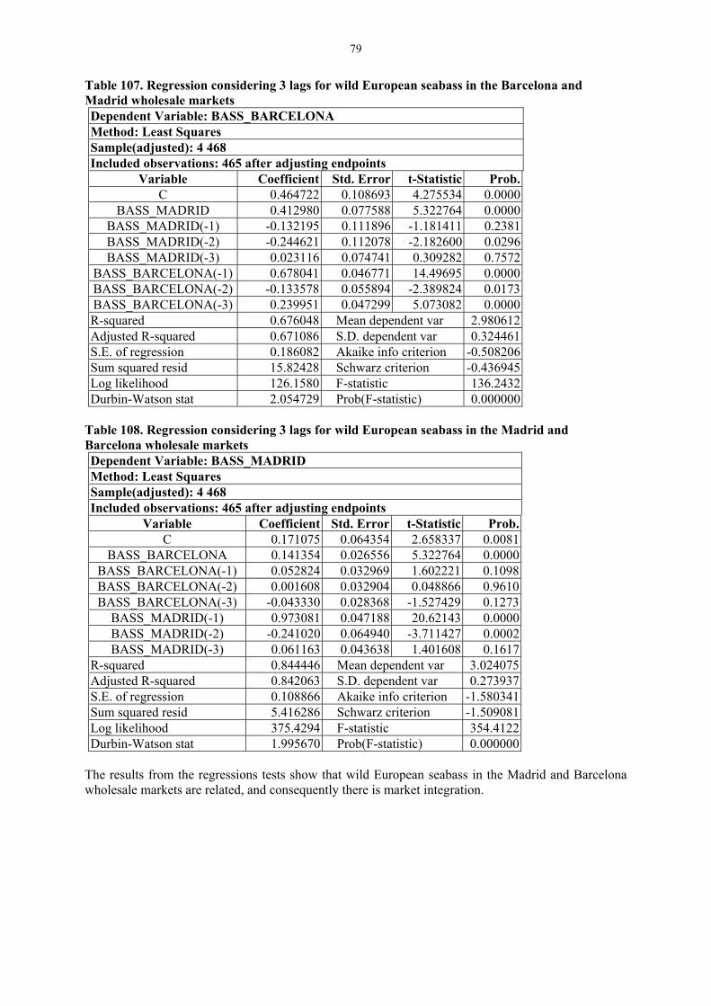
79
Table 107. Regression considering 3 lags for wild European seabass in the Barcelona and Madrid wholesale markets Dependent Variable: BASS_BARCELONA Method: Least Squares Sample(adjusted): 4 468 Included observations: 465 after adjusting endpoints
Variable Coefficient Std. Error t-Statistic Prob. C 0.464722 0.108693 4.275534 0.0000
BASS_MADRID 0.412980 0.077588 5.322764 0.0000 BASS_MADRID(-1) -0.132195 0.111896 -1.181411 0.2381 BASS_MADRID(-2) -0.244621 0.112078 -2.182600 0.0296 BASS_MADRID(-3) 0.023116 0.074741 0.309282 0.7572
BASS_BARCELONA(-1) 0.678041 0.046771 14.49695 0.0000 BASS_BARCELONA(-2) -0.133578 0.055894 -2.389824 0.0173 BASS_BARCELONA(-3) 0.239951 0.047299 5.073082 0.0000 R-squared 0.676048 Mean dependent var 2.980612 Adjusted R-squared 0.671086 S.D. dependent var 0.324461 S.E. of regression 0.186082 Akaike info criterion -0.508206 Sum squared resid 15.82428 Schwarz criterion -0.436945 Log likelihood 126.1580 F-statistic 136.2432 Durbin-Watson stat 2.054729 Prob(F-statistic) 0.000000
Table 108. Regression considering 3 lags for wild European seabass in the Madrid and Barcelona wholesale markets Dependent Variable: BASS_MADRID Method: Least Squares Sample(adjusted): 4 468 Included observations: 465 after adjusting endpoints
Variable Coefficient Std. Error t-Statistic Prob. C 0.171075 0.064354 2.658337 0.0081
BASS_BARCELONA 0.141354 0.026556 5.322764 0.0000 BASS_BARCELONA(-1) 0.052824 0.032969 1.602221 0.1098 BASS_BARCELONA(-2) 0.001608 0.032904 0.048866 0.9610 BASS_BARCELONA(-3) -0.043330 0.028368 -1.527429 0.1273
BASS_MADRID(-1) 0.973081 0.047188 20.62143 0.0000 BASS_MADRID(-2) -0.241020 0.064940 -3.711427 0.0002 BASS_MADRID(-3) 0.061163 0.043638 1.401608 0.1617
R-squared 0.844446 Mean dependent var 3.024075 Adjusted R-squared 0.842063 S.D. dependent var 0.273937 S.E. of regression 0.108866 Akaike info criterion -1.580341 Sum squared resid 5.416286 Schwarz criterion -1.509081 Log likelihood 375.4294 F-statistic 354.4122 Durbin-Watson stat 1.995670 Prob(F-statistic) 0.000000
The results from the regressions tests show that wild European seabass in the Madrid and Barcelona wholesale markets are related, and consequently there is market integration.
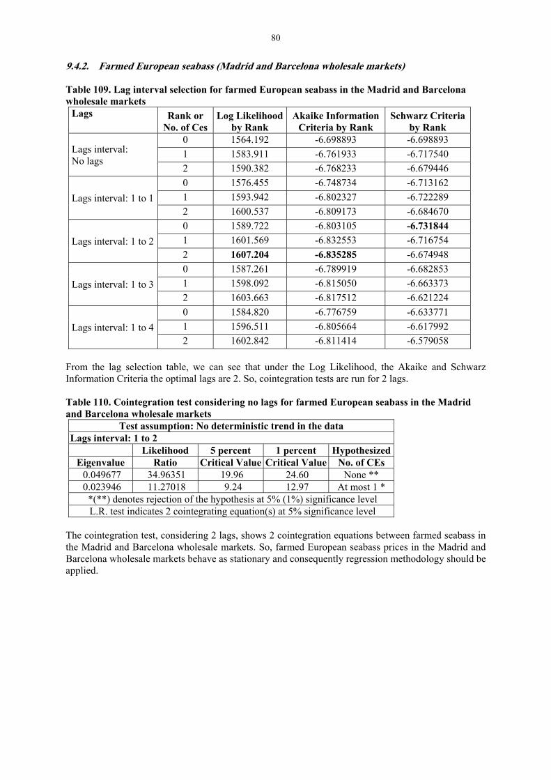
80
9.4.2. Farmed European seabass (Madrid and Barcelona wholesale markets) Table 109. Lag interval selection for farmed European seabass in the Madrid and Barcelona wholesale markets
Lags Rank or No. of Ces
Log Likelihood by Rank
Akaike Information Criteria by Rank
Schwarz Criteria by Rank
Lags interval: No lags
0 1564.192 -6.698893 -6.698893
1 1583.911 -6.761933 -6.717540
2 1590.382 -6.768233 -6.679446
Lags interval: 1 to 1
0 1576.455 -6.748734 -6.713162
1 1593.942 -6.802327 -6.722289
2 1600.537 -6.809173 -6.684670
Lags interval: 1 to 2
0 1589.722 -6.803105 -6.731844
1 1601.569 -6.832553 -6.716754
2 1607.204 -6.835285 -6.674948
Lags interval: 1 to 3
0 1587.261 -6.789919 -6.682853
1 1598.092 -6.815050 -6.663373
2 1603.663 -6.817512 -6.621224
Lags interval: 1 to 4
0 1584.820 -6.776759 -6.633771
1 1596.511 -6.805664 -6.617992
2 1602.842 -6.811414 -6.579058
From the lag selection table, we can see that under the Log Likelihood, the Akaike and Schwarz Information Criteria the optimal lags are 2. So, cointegration tests are run for 2 lags. Table 110. Cointegration test considering no lags for farmed European seabass in the Madrid and Barcelona wholesale markets
Test assumption: No deterministic trend in the data Lags interval: 1 to 2
Likelihood 5 percent 1 percent Hypothesized Eigenvalue Ratio Critical Value Critical Value No. of CEs 0.049677 34.96351 19.96 24.60 None ** 0.023946 11.27018 9.24 12.97 At most 1 *
*(**) denotes rejection of the hypothesis at 5% (1%) significance level L.R. test indicates 2 cointegrating equation(s) at 5% significance level
The cointegration test, considering 2 lags, shows 2 cointegration equations between farmed seabass in the Madrid and Barcelona wholesale markets. So, farmed European seabass prices in the Madrid and Barcelona wholesale markets behave as stationary and consequently regression methodology should be applied.

81
Table 111. Regression considering 2 lags for farmed European seabass in the Barcelona and Madrid wholesale markets Dependent Variable: BASS_BARCELONA Method: Least Squares Sample(adjusted): 3 468 Included observations: 466 after adjusting endpoints
Variable Coefficient Std. Error t-Statistic Prob. C 0.096868 0.035549 2.724952 0.0067
BASS_MADRID 0.081181 0.051874 1.564959 0.1183 BASS_MADRID(-1) -0.078390 0.074278 -1.055350 0.2918 BASS_MADRID(-2) 0.034525 0.051426 0.671358 0.5023
BASS_BARCELONA(-1) 0.717713 0.045981 15.60876 0.0000 BASS_BARCELONA(-2) 0.187920 0.046021 4.083338 0.0001 R-squared 0.855296 Mean dependent var 1.736433 Adjusted R-squared 0.853723 S.D. dependent var 0.120596 S.E. of regression 0.046123 Akaike info criterion -3.302205 Sum squared resid 0.978586 Schwarz criterion -3.248846 Log likelihood 775.4137 F-statistic 543.7810 Durbin-Watson stat 2.040024 Prob(F-statistic) 0.000000
Table 112. Regression considering 2 lags for farmed European seabass in the Madrid and Barcelona wholesale markets Dependent Variable: BASS_MADRID Method: Least Squares Sample(adjusted): 3 468 Included observations: 466 after adjusting endpoints
Variable Coefficient Std. Error t-Statistic Prob. C 0.070784 0.031953 2.215245 0.0272
BASS_BARCELONA 0.065236 0.041686 1.564959 0.1183 BASS_BARCELONA(-1) 0.033443 0.050956 0.656322 0.5119 BASS_BARCELONA(-2) -0.026518 0.041978 -0.631715 0.5279
BASS_MADRID(-1) 1.032020 0.046141 22.36648 0.0000 BASS_MADRID(-2) -0.140097 0.045658 -3.068408 0.0023
R-squared 0.889590 Mean dependent var 1.812092 Adjusted R-squared 0.888390 S.D. dependent var 0.123762 S.E. of regression 0.041347 Akaike info criterion -3.520862 Sum squared resid 0.786388 Schwarz criterion -3.467504 Log likelihood 826.3610 F-statistic 741.2600 Durbin-Watson stat 1.987008 Prob(F-statistic) 0.000000
The results from the regressions tests show that farmed European seabass in the Madrid and Barcelona wholesale markets are not related, and consequently there is no market integration.

82
9.4.3. Farmed European seabass (Madrid and Paris wholesale markets) Table 113. Lag interval selection for farmed European seabass in the Madrid and Paris wholesale markets
Lags Rank or No. of Ces
Log Likelihood by Rank
Akaike Information Criteria by Rank
Schwarz Criteria by Rank
Lags interval: No lags
0 1177.185 -7.719245 -7.719245
1 1183.558 -7.728248 -7.667259
2 1188.516 -7.727976 -7.605999
Lags interval: 1 to 1
0 1173.837 -7.773000 -7.723736
1 1182.205 -7.795382 -7.684538
2 1186.442 -7.790311 -7.617887
Lags interval: 1 to 2
0 1177.288 -7.873992 -7.774497
1 1183.925 -7.885020 -7.723341
2 1186.531 -7.868898 -7.645035
Lags interval: 1 to 3
0 1159.772 -7.834623 -7.683900
1 1165.912 -7.842406 -7.628881
2 1168.003 -7.822546 -7.546219
Lags interval: 1 to 4
0 1143.739 -7.804422 -7.601436
1 1151.790 -7.825536 -7.559118
2 1153.536 -7.803020 -7.473169
From the lag selection table, we can see that under the Log Likelihood the optimal lags are 0, while under the Akaike and Schwarz Information Criteria the optimal lags are 2. So, cointegration tests are run for 0 and 2 lags. Table 114. Cointegration test considering no lags for farmed European seabass in the Madrid and Paris wholesale markets
Test assumption: No deterministic trend in the data Lags interval: No lags
Likelihood 5 percent 1 percent Hypothesized Eigenvalue Ratio Critical Value Critical Value No. of CEs 0.040929 22.66321 19.96 24.60 None * 0.031993 9.917270 9.24 12.97 At most 1 *
*(**) denotes rejection of the hypothesis at 5% (1%) significance level L.R. test indicates 2 cointegrating equation(s) at 5% significance level
Table 115. Cointegration test considering 2 lags for farmed European seabass in the Madrid and Paris wholesale markets
Test assumption: No deterministic trend in the data Lags interval: 1 to 2
Likelihood 5 percent 1 percent Hypothesized Eigenvalue Ratio Critical Value Critical Value No. of CEs 0.043714 18.48710 19.96 24.60 None 0.017395 5.211805 9.24 12.97 At most 1
*(**) denotes rejection of the hypothesis at 5% (1%) significance level L.R. rejects any cointegration at 5% significance level
The cointegration test, considering 0 and 2 lags, shows 2 and 0 cointegration equations respectively between farmed European seabass in the Madrid and Paris wholesale markets. So, when considering 2 lags, farmed European seabass in Madrid and Paris wholesale markets are not cointegrated. Regression methodology is needed to investigate the relationship between both price series when considering 0 lags.

83
Table 116. Regression considering 0 lags for farmed European seabass in the Madrid and Paris wholesale markets Dependent Variable: BASS_MAD Method: Least Squares Date: 09/14/17 Time: 10:55 Sample: 1 312 Included observations: 309 Excluded observations: 3
Variable Coefficient Std. Error t-Statistic Prob. C 2.274403 0.111326 20.43006 0.0000
BASS_FRA -0.220282 0.057083 -3.858960 0.0001 R-squared 0.046263 Mean dependent var 1.845377 Adjusted R-squared 0.043156 S.D. dependent var 0.103755 S.E. of regression 0.101492 Akaike info criterion -1.731228 Sum squared resid 3.162274 Schwarz criterion -1.707064 Log likelihood 269.4747 F-statistic 14.89157 Durbin-Watson stat 0.173312 Prob(F-statistic) 0.000139
Table 117. Regression considering 0 lags for farmed European seabass in the Paris and Madrid wholesale markets Dependent Variable: BASS_FRA Method: Least Squares Sample: 1 312 Included observations: 309 Excluded observations: 3
Variable Coefficient Std. Error t-Statistic Prob. C 2.335180 0.100589 23.21507 0.0000
BASS_MAD -0.210016 0.054423 -3.858960 0.0001 R-squared 0.046263 Mean dependent var 1.947621 Adjusted R-squared 0.043156 S.D. dependent var 0.101309 S.E. of regression 0.099099 Akaike info criterion -1.778952 Sum squared resid 3.014902 Schwarz criterion -1.754788 Log likelihood 276.8481 F-statistic 14.89157 Durbin-Watson stat 0.103077 Prob(F-statistic) 0.000139
The results from the regression tests show that farmed European seabass in the Paris and Madrid wholesale markets are related when considering 0 lags; however, the explanatory potential (R-squared) is very low, so the relation seems very weak. Consequently, the existence of market integration between farmed European seabass from the Madrid and Paris wholesale markets is uncertain as we obtain different results when considering different lags.
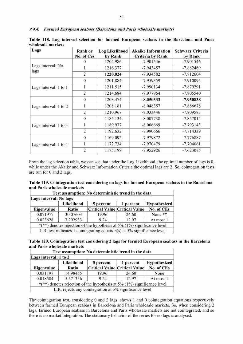
84
9.4.4. Farmed European seabass (Barcelona and Paris wholesale markets) Table 118. Lag interval selection for farmed European seabass in the Barcelona and Paris wholesale markets
Lags Rank or No. of Ces
Log Likelihood by Rank
Akaike Information Criteria by Rank
Schwarz Criteria by Rank
Lags interval: No lags
0 1204.986 -7.901546 -7.901546
1 1216.377 -7.943457 -7.882469
2 1220.024 -7.934582 -7.812604
Lags interval: 1 to 1
0 1201.884 -7.959359 -7.910095
1 1211.515 -7.990134 -7.879291
2 1214.684 -7.977964 -7.805540
Lags interval: 1 to 2
0 1203.474 -8.050333 -7.950838
1 1208.181 -8.048357 -7.886678
2 1210.967 -8.033446 -7.809583
Lags interval: 1 to 3
0 1185.134 -8.007738 -7.857014
1 1189.977 -8.006669 -7.793143
2 1192.632 -7.990666 -7.714339
Lags interval: 1 to 4
0 1169.092 -7.979872 -7.776887
1 1172.734 -7.970479 -7.704061
2 1175.198 -7.952926 -7.623075
From the lag selection table, we can see that under the Log Likelihood, the optimal number of lags is 0, while under the Akaike and Schwarz Information Criteria the optimal lags are 2. So, cointegration tests are run for 0 and 2 lags. Table 119. Cointegration test considering no lags for farmed European seabass in the Barcelona and Paris wholesale markets
Test assumption: No deterministic trend in the data Lags interval: No lags
Likelihood 5 percent 1 percent Hypothesized Eigenvalue Ratio Critical Value Critical Value No. of CEs 0.071977 30.07603 19.96 24.60 None ** 0.023628 7.292933 9.24 12.97 At most 1
*(**) denotes rejection of the hypothesis at 5% (1%) significance level L.R. test indicates 1 cointegrating equation(s) at 5% significance level
Table 120. Cointegration test considering 2 lags for farmed European seabass in the Barcelona and Paris wholesale markets
Test assumption: No deterministic trend in the data Lags interval: 1 to 2
Likelihood 5 percent 1 percent Hypothesized Eigenvalue Ratio Critical Value Critical Value No. of CEs 0.031197 14.98455 19.96 24.60 None 0.018584 5.571356 9.24 12.97 At most 1
*(**) denotes rejection of the hypothesis at 5% (1%) significance level L.R. rejects any cointegration at 5% significance level
The cointegration test, considering 0 and 2 lags, shows 1 and 0 cointegration equations respectively between farmed European seabass in Barcelona and Paris wholesale markets. So, when considering 2 lags, farmed European seabass in Barcelona and Paris wholesale markets are not cointegrated, and so there is no market integration. The stationary behavior of the series for no lags is analysed.

85
Table 121. Unit root test considering intercept and no lags for farmed European seabass in the Barcelona and Paris wholesale markets Series Lags ADF Test
Statistic Critical Values
Bass at Barcelona 0 -2.894261 1%: -3.4532 5%: -2.8710 10%: -2.5718 Bass at Paris 0 -2.960999 1%: -3.4536 5%: -2.8712 10%: -2.5719
The ADF Test statistics for farmed European seabass in the Barcelona and Paris wholesale markets considering no lags are lower than the MacKinnon critical value for rejection of the hypothesis of a unit root at a 5% significance level. So, both price series behave as a stationary series when considering no lags. There is a contradiction between the ADF test and the cointegration test results when considering no lags, because according to the ADF test there should be 0 cointegration equations since both series are stationary. This could be in part explained because the ADF Test statistic value is close to the critical value. Table 122. Regression considering no lags for farmed European seabass in the Barcelona and Paris wholesale markets Dependent Variable: Bass at Barcelona Method: Least Squares Sample: 1 312 Included observations: 309 Excluded observations: 3
Variable Coefficient Std. Error t-Statistic Prob. C 2.772808 0.111083 24.96169 0.0000
Bass at Paris -0.521618 0.056958 -9.157914 0.0000 R-squared 0.214567 Mean dependent var 1.756892 Adjusted R-squared 0.212009 S.D. dependent var 0.114082 S.E. of regression 0.101269 Akaike info criterion -1.735612 Sum squared resid 3.148440 Schwarz criterion -1.711448 Log likelihood 270.1521 F-statistic 83.86739 Durbin-Watson stat 0.159656 Prob(F-statistic) 0.000000
Table 123. Regression considering no lag for farmed European seabass in the Paris and Barcelona wholesale markets Dependent Variable: Bass at Paris Method: Least Squares Sample: 1 312 Included observations: 309 Excluded observations: 3
Variable Coefficient Std. Error t-Statistic Prob. C 2.670318 0.079081 33.76703 0.0000
Bass at Barcelona -0.411349 0.044917 -9.157914 0.0000 R-squared 0.214567 Mean dependent var 1.947621 Adjusted R-squared 0.212009 S.D. dependent var 0.101309 S.E. of regression 0.089931 Akaike info criterion -1.973106 Sum squared resid 2.482866 Schwarz criterion -1.948942 Log likelihood 306.8448 F-statistic 83.86739 Durbin-Watson stat 0.138909 Prob(F-statistic) 0.000000
The results from the regression tests show that farmed European seabass in the Paris and Barcelona wholesale markets are related when considering no lags, and so there is market integration. Consequently, the existence of market integration between farmed European seabass from the Barcelona and Paris wholesale markets is uncertain as we obtain different results when considering different lags.

86
9.4.5. Farmed European seabass (Turkish Exports and Madrid wholesale market) Table 124. Lag interval selection for farmed European seabass imported to the EU from Turkey and the Madrid wholesale market
Lags Rank or No. of Ces
Log Likelihood by Rank
Akaike Information Criteria by Rank
Schwarz Criteria by Rank
Lags interval: No lags
0 829.3961 -8.013489 -8.013489
1 836.0907 -8.029862 -7.949361
2 841.2962 -8.031848 -7.870847
Lags interval: 1 to 1
0 835.7022 -8.074778 -8.010159
1 842.6236 -8.093433 -7.948040
2 846.3126 -8.080704 -7.854538
Lags interval: 1 to 2
0 836.5827 -8.083734 -7.954055
1 841.9984 -8.087789 -7.877062
2 845.0587 -8.068865 -7.777089
Lags interval: 1 to 3
0 832.5601 -8.044707 -7.849524
1 837.8187 -8.047242 -7.770732
2 840.8140 -8.027589 -7.669752
Lags interval: 1 to 4
0 834.4810 -8.063852 -7.802713
1 840.0906 -8.069859 -7.727113
2 843.1619 -8.050856 -7.626504
From the lag selection table, we can see that under the Log Likelihood and the Schwarz Information Criteria the optimal lag is 1, while under the Schwarz Information Criteria the optimal lag is 0. So, cointegration tests are run for 0 and 1 lags. Table 125. Cointegration test considering no lags for farmed European seabass imported to the EU from Turkey and the Madrid wholesale market
Test assumption: No deterministic trend in the data Lags interval: No lags
Likelihood 5 percent 1 percent Hypothesized Eigenvalue Ratio Critical Value Critical Value No. of CEs 0.062635 23.80025 19.96 24.60 None * 0.049051 10.41105 9.24 12.97 At most 1 *
*(**) denotes rejection of the hypothesis at 5% (1%) significance level L.R. test indicates 2 cointegrating equation(s) at 5% significance level
Table 126. Cointegration test considering 1 lag for farmed European seabass imported to the EU from Turkey and the Madrid wholesale market
Test assumption: No deterministic trend in the data Lags interval: 1 to 1
Likelihood 5 percent 1 percent Hypothesized Eigenvalue Ratio Critical Value Critical Value No. of CEs 0.064990 21.22076 19.96 24.60 None * 0.035181 7.377945 9.24 12.97 At most 1
*(**) denotes rejection of the hypothesis at 5% (1%) significance level L.R. test indicates 1 cointegrating equation(s) at 5% significance level

87
The cointegration test, considering 0 and 1 lags, shows 2 and 1 cointegration equations respectively, between farmed imported to the EU from Turkey and from the Madrid wholesale market. So, prices of farmed European seabass imported to the EU from Turkey and from the Madrid wholesale market behave as stationary series, and consequently regression methodology needs to be applied in order to assess market integrated when considering no lags. Instead, when considering 1 lag, the stationary behavior of the series needs to be further analysed. Table 127. Unit root test considering intercept and 1 lag for farmed European seabass imported to the EU from Turkey and from the Madrid wholesale market Series Lags ADF Test Statistic Critical Values Turkish exports 1 -2.600862 1%: -3.4634 5%: -2.8756 10%: -2.5742 Madrid wholesale market 1 -3.516019 1%: -3.4634 5%: -2.8756 10%: -2.5742
The ADF Test statistics for farmed European seabass imported to the EU from Turkey are higher than the MacKinnon critical value for rejection of the hypothesis of a unit root at a 5% significance level. So, the farmed European seabass imported to the EU from the Turkish price series behaves as a non-stationary series. While farmed European seabass from the Madrid wholesale market behaves as stationary when considering 1 lag. Consequently, there is also no market integration between farmed European seabass imported to the EU from Turkey and from the Madrid wholesale market when considering 1 lag. Table 128. Regression considering 0 lags for farmed European seabass in the Madrid wholesale market and exports from Turkey Dependent Variable: BASS_MADRID Method: Least Squares Sample: 1 208 Included observations: 208
Variable Coefficient Std. Error t-Statistic Prob. C 0.860285 0.101740 8.455730 0.0000
BASS_TURKEY 0.640074 0.065085 9.834475 0.0000 R-squared 0.319496 Mean dependent var 1.859320 Adjusted R-squared 0.316193 S.D. dependent var 0.097871 S.E. of regression 0.080932 Akaike info criterion -2.180842 Sum squared resid 1.349304 Schwarz criterion -2.148750 Log likelihood 228.8075 F-statistic 96.71690 Durbin-Watson stat 0.224902 Prob(F-statistic) 0.000000
Table 129. Regression considering 0 lags for farmed European seabass exports from Turkey and in the Madrid wholesale market Dependent Variable: BASS_TURKEY Method: Least Squares Sample: 1 208 Included observations: 208
Variable Coefficient Std. Error t-Statistic Prob. C 0.632723 0.094501 6.695409 0.0000
BASS_MADRID 0.499155 0.050756 9.834475 0.0000 R-squared 0.319496 Mean dependent var 1.560813 Adjusted R-squared 0.316193 S.D. dependent var 0.086429 S.E. of regression 0.071470 Akaike info criterion -2.429507 Sum squared resid 1.052242 Schwarz criterion -2.397416 Log likelihood 254.6688 F-statistic 96.71690 Durbin-Watson stat 0.205592 Prob(F-statistic) 0.000000

88
The results from the regressions tests show that farmed European seabass imported to the EU from Turkey and from the Madrid wholesale market are related (i.e., there is market integration) when considering no lags. Consequently, the existence of market integration between farmed European seabass imported to the EU from Turkey and from the Madrid wholesale market is uncertain as we obtain different results when considering different lags. 9.4.6. Farmed European seabass (Turkish Exports and Barcelona wholesale market) Table 130. Lag interval selection for farmed European seabass imported to the EU from Turkey and the Barcelona wholesale market
Lags Rank or No. of CEs
Log Likelihood by Rank
Akaike Information Criteria by Rank
Schwarz Criteria by Rank
Lags interval: No lags
0 827.0397 -7.990722 -7.990722
1 838.7500 -8.055555 -7.975055
2 843.4889 -8.053033 -7.892032
Lags interval: 1 to 1
0 839.3099 -8.109805 -8.045186
1 845.9192 -8.125429 -7.980037
2 849.2732 -8.109448 -7.883282
Lags interval: 1 to 2
0 838.5826 -8.103245 -7.973567
1 843.8821 -8.106167 -7.895439
2 847.0668 -8.088456 -7.796680
Lags interval: 1 to 3
0 835.2228 -8.070811 -7.875628
1 840.5845 -8.074358 -7.797848
2 843.6505 -8.055397 -7.697561
Lags interval: 1 to 4
0 838.1064 -8.099570 -7.838431
1 843.5299 -8.103743 -7.760997
2 846.5775 -8.084508 -7.660156
From the lag selection table, we can see that under the Log Likelihood, the Akaike and Schwarz Information Criteria the optimal lags is 1. So, cointegration tests are run for 1 lag. Table 131. Cointegration test considering 1 lag for farmed European seabass imported to the EU from Turkey and from the Barcelona wholesale market
Test assumption: No deterministic trend in the data Lags interval: 1 to 1
Likelihood 5 percent 1 percent Hypothesized Eigenvalue Ratio Critical Value Critical Value No. of CEs 0.062152 19.92650 19.96 24.60 None 0.032038 6.707962 9.24 12.97 At most 1
*(**) denotes rejection of the hypothesis at 5% (1%) significance level L.R. rejects any cointegration at 5% significance level
The cointegration test, considering 1 lag, shows 0 cointegration equations between farmed European seabass imported to the EU from Turkey and from the Barcelona wholesale market. Therefore, there is no market integration between farmed European seabass imported to the EU from Turkey and from the Barcelona wholesale market.

89
9.4.7. Farmed European seabass (Turkish Exports and Paris wholesale market) Table 132. Lag interval selection for farmed European seabass imported to the EU from Turkey and the Paris wholesale market
Lags Rank or No. of CEs
Log Likelihood by Rank
Akaike Information Criteria by Rank
Schwarz Criteria by Rank
Lags interval: No lags
0 884.8164 -8.632355 -8.632355
1 890.7351 -8.641318 -8.560269
2 894.1361 -8.625718 -8.463620
Lags interval: 1 to 1
0 881.5881 -8.646188 -8.580904
1 887.1536 -8.651760 -8.504869
2 889.8492 -8.629056 -8.400559
Lags interval: 1 to 2
0 875.4429 -8.631273 -8.499798
1 880.5987 -8.632823 -8.419176
2 882.6282 -8.603266 -8.307447
Lags interval: 1 to 3
0 866.7394 -8.590345 -8.391754
1 872.7517 -8.600519 -8.319182
2 874.4803 -8.567641 -8.203557
Lags interval: 1 to 4
0 862.0817 -8.589662 -8.323006
1 867.6539 -8.595471 -8.245484
2 870.1564 -8.570116 -8.136799
From the lag selection table, we can see that under the Log Likelihood and the Schwarz Information Criteria the optimal lags are 0 lags, while under the Akaike Information Criteria the optimal lags is 1. In this case, cointegration tests are run for 0 and 1 lags. Table 133. Cointegration test considering no lags for farmed European seabass imported to the EU from Turkey and from the Paris wholesale market
Test assumption: No deterministic trend in the data Lags interval: No lags
Likelihood 5 percent 1 percent Hypothesized Eigenvalue Ratio Critical Value Critical Value No. of CEs 0.056108 18.63931 19.96 24.60 None 0.032636 6.801959 9.24 12.97 At most 1
*(**) denotes rejection of the hypothesis at 5% (1%) significance level L.R. rejects any cointegration at 5% significance level
Table 134. Cointegration test considering 1 lag for farmed European seabass imported to the EU from Turkey and from the Paris wholesale market
Test assumption: No deterministic trend in the data Lags interval: 1 to 1
Likelihood 5 percent 1 percent Hypothesized Eigenvalue Ratio Critical Value Critical Value No. of CEs 0.053356 16.52213 19.96 24.60 None 0.026208 5.391114 9.24 12.97 At most 1
*(**) denotes rejection of the hypothesis at 5% (1%) significance level L.R. rejects any cointegration at 5% significance level

90
The cointegration tests, considering 0 and 1 lags, shows 0 cointegration equations between farmed European seabass imported to the EU from Turkey and from the Paris wholesale market. Therefore, there is no market integration between farmed European seabass imported to the EU from Turkey and from the Paris wholesale market. 9.4.8. Wild gilthead seabream (Madrid and Barcelona wholesale markets) Table 135. Lag interval selection for wild gilthead seabream in the Madrid and Barcelona wholesale markets
Lags Rank or No. of CEs
Log Likelihood by Rank
Akaike Information Criteria by Rank
Schwarz Criteria by Rank
Lags interval: No lags
0 691.6580 -3.7387 -3.7387
1 717.3198 -3.8504 -3.7975
2 719.2755 -3.8339 -3.7282
Lags interval: 1 to 1
0 654.5822 -3.7176 -3.6735
1 679.3939 -3.8308 -3.7316
2 681.9001 -3.8166 -3.6623
Lags interval: 1 to 2
0 613.0281 -3.6447 -3.5531
1 637.6333 -3.7629 -3.6139
2 639.9293 -3.7466 -3.5403
Lags interval: 1 to 3
0 581.2535 -3.6258 -3.4825
1 601.1125 -3.7205 -3.5175
2 603.0785 -3.7011 -3.4384
Lags interval: 1 to 4
0 545.6293 -3.5786 -3.3791
1 558.5662 -3.6322 -3.3704
2 560.5839 -3.6121 -3.2879
From the lag selection table, we can see that under the Log Likelihood, the Akaike and Schwarz Information Criteria the optimal lags are 0. So, cointegration tests are run for 0 lags. Table 136. Cointegration test considering 0 lags for wild gilthead seabream in the Madrid and Barcelona wholesale markets
Test assumption: No deterministic trend in the data Lags interval: No lags
Likelihood 5 percent 1 percent Hypothesized Eigenvalue Ratio Critical Value Critical Value No. of CEs 0.129522 55.23486 19.96 24.60 None ** 0.010515 3.911290 9.24 12.97 At most 1
*(**) denotes rejection of the hypothesis at 5% (1%) significance level L.R. test indicates 1 cointegrating equation(s) at 5% significance level
The cointegration test, considering 0 lags, shows 1 cointegration equation between wild gilthead seabream in the Madrid and Barcelona wholesale markets. So the stationary behavior of the series is analysed.

91
Table 137 Unit root test considering intercept and 0 lags for wild gilthead seabream in the Madrid and Barcelona wholesale markets Series Lags ADF Test
Statistic Critical Values
Wild seabream Madrid 0 -1.606148 1%: -3.4500 5%: -2.8696 10%: -2.5710 Wild seabream Barcelona 0 -8.076360 1%: -3.4466 5%: -2.8680 10%: -2.5702
The ADF Test Statistic for wild seabream in the Madrid wholesale market is higher than the MacKinnon critical value for rejection of the hypothesis of a unit root at a 5% significance level. So, the wild seabream in the Mercamadrid price series behaves as a non-stationary series. While wild seabream in the Mercabarna price series behaves as stationary. Therefore, there is no market integration between wild seabream in the Madrid and Barcelona wholesale markets. 9.4.9. Farmed gilthead seabream (Madrid and Barcelona wholesale markets) Table 138. Lag interval selection for farmed gilthead seabream in the Madrid and Barcelona wholesale markets
Lags Rank or No. of CEs
Log Likelihood by Rank
Akaike Information Criteria by Rank
Schwarz Criteria by Rank
Lags interval: No lags
0 1667.538 -7.141492 -7.141492
1 1681.957 -7.181828 -7.137435
2 1684.546 -7.171505 -7.082719
Lags interval: 1 to 1
0 1679.810 -7.192319 -7.156747
1 1690.799 -7.218022 -7.137985
2 1693.868 -7.209732 -7.085229
Lags interval: 1 to 2
0 1687.379 -7.223135 -7.151874
1 1695.195 -7.235247 -7.119448
2 1698.628 -7.228508 -7.068171
Lags interval: 1 to 3
0 1689.970 -7.232631 -7.125565
1 1696.926 -7.241060 -7.089383
2 1701.245 -7.238123 -7.041836
Lags interval: 1 to 4
0 1687.996 -7.222443 -7.079455
1 1695.356 -7.232638 -7.044966
2 1700.465 -7.233109 -7.000753
From the lag selection table, we can see that under the Log Likelihood and the Akaike Information Criteria the optimal lags are 3, while under the Schwarz Information Criteria the optimal lag is 1. In this case, cointegration tests are run for 1 and 3 lags. Table 139. Cointegration test considering 1 lag for farmed gilthead seabream in the Madrid and Barcelona wholesale markets
Test assumption: No deterministic trend in the data Lags interval: 1 to 1
Likelihood 5 percent 1 percent Hypothesized Eigenvalue Ratio Critical Value Critical Value No. of CEs 0.046067 28.11443 19.96 24.60 None ** 0.013083 6.136806 9.24 12.97 At most 1
*(**) denotes rejection of the hypothesis at 5% (1%) significance level L.R. test indicates 1 cointegrating equation(s) at 5% significance level
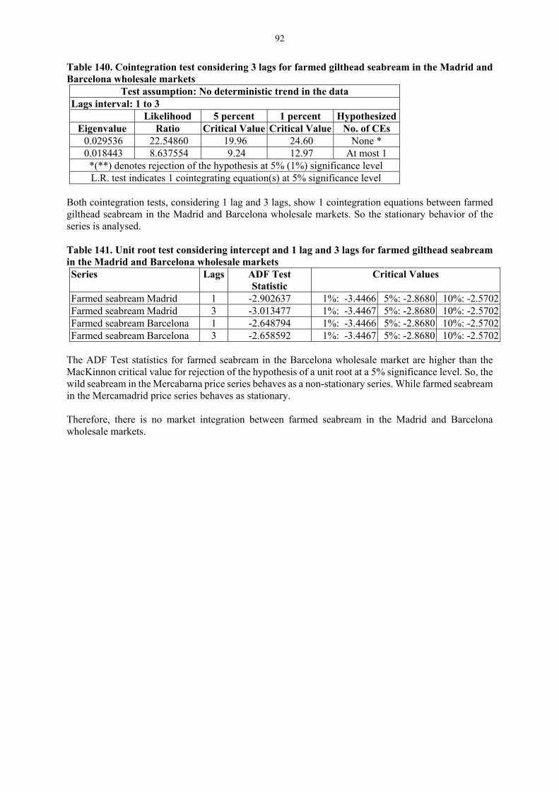
92
Table 140. Cointegration test considering 3 lags for farmed gilthead seabream in the Madrid and Barcelona wholesale markets
Test assumption: No deterministic trend in the data Lags interval: 1 to 3
Likelihood 5 percent 1 percent Hypothesized Eigenvalue Ratio Critical Value Critical Value No. of CEs 0.029536 22.54860 19.96 24.60 None * 0.018443 8.637554 9.24 12.97 At most 1
*(**) denotes rejection of the hypothesis at 5% (1%) significance level L.R. test indicates 1 cointegrating equation(s) at 5% significance level
Both cointegration tests, considering 1 lag and 3 lags, show 1 cointegration equations between farmed gilthead seabream in the Madrid and Barcelona wholesale markets. So the stationary behavior of the series is analysed. Table 141. Unit root test considering intercept and 1 lag and 3 lags for farmed gilthead seabream in the Madrid and Barcelona wholesale markets Series Lags ADF Test
Statistic Critical Values
Farmed seabream Madrid 1 -2.902637 1%: -3.4466 5%: -2.8680 10%: -2.5702 Farmed seabream Madrid 3 -3.013477 1%: -3.4467 5%: -2.8680 10%: -2.5702 Farmed seabream Barcelona 1 -2.648794 1%: -3.4466 5%: -2.8680 10%: -2.5702 Farmed seabream Barcelona 3 -2.658592 1%: -3.4467 5%: -2.8680 10%: -2.5702
The ADF Test statistics for farmed seabream in the Barcelona wholesale market are higher than the MacKinnon critical value for rejection of the hypothesis of a unit root at a 5% significance level. So, the wild seabream in the Mercabarna price series behaves as a non-stationary series. While farmed seabream in the Mercamadrid price series behaves as stationary. Therefore, there is no market integration between farmed seabream in the Madrid and Barcelona wholesale markets.

93
9.4.10. Farmed gilthead seabream (Madrid and Paris wholesale markets) Table 142. Lag interval selection for farmed gilthead seabream in the Madrid and Paris wholesale markets
Lags Rank or No. of CEs
Log Likelihood by Rank
Akaike Information Criteria by Rank
Schwarz Criteria by Rank
Lags interval: No lags
0 1092.863 -7.166317 -7.166317
1 1097.758 -7.165628 -7.104639
2 1101.558 -7.157760 -7.035782
Lags interval: 1 to 1
0 1097.116 -7.263231 -7.213967
1 1101.574 -7.259626 -7.148782
2 1105.344 -7.251457 -7.079033
Lags interval: 1 to 2
0 1097.483 -7.336583 -7.237089
1 1100.604 -7.323935 -7.162256
2 1103.139 -7.307336 -7.083473
Lags interval: 1 to 3
0 1080.907 -7.296294 -7.145571
1 1083.750 -7.281569 -7.068043
2 1086.379 -7.265384 -6.989057
Lags interval: 1 to 4
0 1071.679 -7.305737 -7.102751
1 1075.432 -7.297107 -7.030688
2 1077.500 -7.276815 -6.946964
From the lag selection table, we can see that under the Log Likelihood the optimal lags length is 1 lag, while under the Akaike and Schwarz Information Criteria the optimal lags are 2. So, cointegration tests are run for 1 and 2 lags. Table 143. Cointegration test considering 1 lag for farmed gilthead seabream in the Madrid and Paris wholesale markets
Test assumption: No deterministic trend in the data Lags interval: 1 to 1
Likelihood 5 percent 1 percent Hypothesized Eigenvalue Ratio Critical Value Critical Value No. of CEs 0.029183 16.45605 19.96 24.60 None 0.024743 7.541262 9.24 12.97 At most 1
*(**) denotes rejection of the hypothesis at 5% (1%) significance level L.R. rejects any cointegration at 5% significance level
Table 144. Cointegration test considering 2 lags for farmed gilthead seabream in the Madrid and Paris wholesale markets
Test assumption: No deterministic trend in the data Lags interval: 1 to 2
Likelihood 5 percent 1 percent Hypothesized Eigenvalue Ratio Critical Value Critical Value No. of CEs 0.020802 11.31347 19.96 24.60 None 0.016926 5.070066 9.24 12.97 At most 1
*(**) denotes rejection of the hypothesis at 5% (1%) significance level L.R. rejects any cointegration at 5% significance level
Cointegration tests, considering 1 and 2 lags, show 0 cointegration equations between farmed gilthead seabream in the Madrid and Paris wholesale markets. Therefore, there is no market integration between farmed gilthead seabream in the Madrid and Paris wholesale markets.

94
9.4.11. Farmed gilthead seabream (Barcelona and Paris wholesale markets) Table 145. Lag interval selection for farmed gilthead seabream in the Barcelona and Paris wholesale markets
Lags Rank or No. of CEs
Log Likelihood by Rank
Akaike Information Criteria by Rank
Schwarz Criteria by Rank
Lags interval: No lags
0 1102.745 -7.231115 -7.231115
1 1108.068 -7.233234 -7.172245
2 1111.789 -7.224847 -7.102870
Lags interval: 1 to 1
0 1118.619 -7.406105 -7.356841
1 1122.859 -7.401059 -7.290215
2 1125.665 -7.386480 -7.214057
Lags interval: 1 to 2
0 1118.052 -7.475098 -7.375604
1 1120.605 -7.458619 -7.296941
2 1122.535 -7.437945 -7.214082
Lags interval: 1 to 3
0 1102.512 -7.443767 -7.293043
1 1105.448 -7.429679 -7.216154
2 1107.454 -7.409245 -7.132918
Lags interval: 1 to 4
0 1093.459 -7.456465 -7.253479
1 1096.780 -7.444846 -7.178427
2 1098.727 -7.423718 -7.093867
From the lag selection table, we can see that under the Log Likelihood the optimal lags length is 1 lag, while under the Akaike and the Schwarz Information Criteria the optimal lags are 2. So, cointegration tests are run for 1 and 2 lags. Table 146. Cointegration test considering 1 lag for farmed gilthead seabream in the Barcelona and Paris wholesale markets
Test assumption: No deterministic trend in the data Lags interval: 1 to 1
Likelihood 5 percent 1 percent Hypothesized Eigenvalue Ratio Critical Value Critical Value No. of CEs 0.027783 14.09299 19.96 24.60 None 0.018472 5.611916 9.24 12.97 At most 1
*(**) denotes rejection of the hypothesis at 5% (1%) significance level L.R. rejects any cointegration at 5% significance level
Table 147. Cointegration test considering 2 lags for farmed gilthead seabream in the Barcelona and Paris wholesale markets
Test assumption: No deterministic trend in the data Lags interval: 1 to 2
Likelihood 5 percent 1 percent Hypothesized Eigenvalue Ratio Critical Value Critical Value No. of CEs 0.017044 8.965332 19.96 24.60 None 0.012911 3.859605 9.24 12.97 At most 1
*(**) denotes rejection of the hypothesis at 5% (1%) significance level L.R. rejects any cointegration at 5% significance level
Cointegration tests, considering 1 and 2 lags, show 0 cointegration equations between farmed gilthead seabream in the Barcelona and Paris wholesale markets. Therefore, there is no market integration between farmed gilthead seabream in the Barcelona and Paris wholesale markets.

95
9.4.12. Wild turbot (Madrid and Barcelona wholesale markets) Table 148. Lag interval selection for wild turbot in the Madrid and Barcelona wholesale markets
Lags Rank or No. of CEs
Log Likelihood by Rank
Akaike Information Criteria by Rank
Schwarz Criteria by Rank
Lags interval: No lags
0 892.5112 -3.822318 -3.822318
1 936.4712 -3.989170 -3.944777
2 940.7889 -3.986248 -3.897461
Lags interval: 1 to 1
0 911.5230 -3.894949 -3.859376
1 949.9413 -4.038375 -3.958337
2 957.3513 -4.048718 -3.924215
Lags interval: 1 to 2
0 916.4777 -3.907431 -3.836170
1 948.6915 -4.024480 -3.908681
2 955.2178 -4.031044 -3.870707
Lags interval: 1 to 3
0 921.2674 -3.919256 -3.812190
1 946.6449 -4.007090 -3.855413
2 953.1593 -4.013618 -3.817330
Lags interval: 1 to 4
0 925.4626 -3.928564 -3.785576
1 947.4193 -4.001811 -3.814139
2 953.2964 -4.005600 -3.773244
From the lag selection table, we can see that under the Log Likelihood, the Akaike and Schwarz Information Criteria the optimal lag is 1. So, cointegration tests are run considering 1 lag. Table 149. Cointegration test considering 1 lag for wild turbot in the Madrid and Barcelona wholesale markets
Test assumption: No deterministic trend in the data Lags interval: 1 to 1
Likelihood 5 percent 1 percent Hypothesized Eigenvalue Ratio Critical Value Critical Value No. of CEs 0.152009 91.65661 19.96 24.60 None ** 0.031302 14.82002 9.24 12.97 At most 1 **
*(**) denotes rejection of the hypothesis at 5% (1%) significance level L.R. test indicates 2 cointegrating equation(s) at 5% significance level
The cointegration test, considering 1 lag, shows 2 cointegration equations between wild turbot in the Madrid and Barcelona wholesale markets. So, wild turbot prices in the Madrid and Barcelona wholesale markets behave as stationary and consequently regression methodology should be applied.

96
Table 150. Regression considering 1 lag for wild turbot in the Barcelona and Madrid wholesale markets Dependent Variable: TURBOT_BARCELONA Method: Least Squares Sample(adjusted): 2 468 Included observations: 467 after adjusting endpoints
Variable Coefficient Std. Error t-Statistic Prob. C 0.565594 0.127473 4.436955 0.0000
TURBOT_MADRID 0.215311 0.140963 1.527428 0.1273 TURBOT_MADRID(-1) -0.102346 0.139538 -0.733461 0.4636
TURBOT_BARCELONA(-1) 0.682670 0.034650 19.70190 0.0000 R-squared 0.530322 Mean dependent var 2.899354 Adjusted R-squared 0.527279 S.D. dependent var 0.224815 S.E. of regression 0.154571 Akaike info criterion -0.887799 Sum squared resid 11.06208 Schwarz criterion -0.852284 Log likelihood 211.3010 F-statistic 174.2607 Durbin-Watson stat 1.993341 Prob(F-statistic) 0.000000
Table 151. Regression considering 1 lag for wild turbot in the Madrid and Barcelona wholesale markets Dependent Variable: TURBOT_MADRID Method: Least Squares Sample(adjusted): 2 468 Included observations: 467 after adjusting endpoints
Variable Coefficient Std. Error t-Statistic Prob. C 0.040595 0.042761 0.949345 0.3429
TURBOT_BARCELONA 0.023286 0.015245 1.527428 0.1273 TURBOT_BARCELONA(-1) 0.019720 0.015423 1.278612 0.2017
TURBOT_MADRID(-1) 0.947338 0.013034 72.68390 0.0000 R-squared 0.932853 Mean dependent var 3.138968 Adjusted R-squared 0.932418 S.D. dependent var 0.195535 S.E. of regression 0.050832 Akaike info criterion -3.112041 Sum squared resid 1.196357 Schwarz criterion -3.076526 Log likelihood 730.6615 F-statistic 2144.099 Durbin-Watson stat 1.501682 Prob(F-statistic) 0.000000
The results from the regressions tests show that wild turbot in the Madrid and Barcelona wholesale markets are not related, and consequently there is no market integration.

97
9.4.13. Farmed turbot (Madrid and Barcelona wholesale markets) Table 152. Lag interval selection for farmed turbot in the Madrid and Barcelona wholesale markets
Lags Rank or No. of CEs
Log Likelihood by Rank
Akaike Information Criteria by Rank
Schwarz Criteria by Rank
Lags interval: No lags
0 1717.521 -7.355548 -7.355548
1 1727.894 -7.378561 -7.334167
2 1730.468 -7.368172 -7.279386
Lags interval: 1 to 1
0 1723.014 -7.377742 -7.342170
1 1733.567 -7.401575 -7.321537
2 1736.805 -7.394012 -7.269509
Lags interval: 1 to 2
0 1720.947 -7.367514 -7.296253
1 1732.344 -7.395026 -7.279227
2 1735.125 -7.385486 -7.225149
Lags interval: 1 to 3
0 1720.340 -7.363536 -7.256470
1 1731.448 -7.389861 -7.238184
2 1734.866 -7.383045 -7.186757
Lags interval: 1 to 4
0 1716.275 -7.344598 -7.201610
1 1727.177 -7.370095 -7.182423
2 1730.512 -7.362904 -7.130548
From the lag selection table, we can see that under the Log Likelihood and the Akaike Information Criteria the optimal lag is 1; while under the Schwarz Information Criteria the optimal lags are 0. In this case, cointegration tests are run for 0 and 1 lag. Table 153. Cointegration test considering 0 lags for farmed turbot in the Madrid and Barcelona wholesale markets
Test assumption: No deterministic trend in the data Lags interval: No lags
Likelihood 5 percent 1 percent Hypothesized Eigenvalue Ratio Critical Value Critical Value No. of CEs 0.043453 25.89533 19.96 24.60 None ** 0.010964 5.148573 9.24 12.97 At most 1
*(**) denotes rejection of the hypothesis at 5% (1%) significance level L.R. test indicates 1 cointegrating equation(s) at 5% significance level
Table 154. Cointegration test considering 1 lag for farmed turbot in the Madrid and Barcelona wholesale markets
Test assumption: No deterministic trend in the data Lags interval: 1 to 1
Likelihood 5 percent 1 percent Hypothesized Eigenvalue Ratio Critical Value Critical Value No. of CEs 0.044282 27.58173 19.96 24.60 None ** 0.013800 6.475534 9.24 12.97 At most 1
*(**) denotes rejection of the hypothesis at 5% (1%) significance level L.R. test indicates 1 cointegrating equation(s) at 5% significance level
Both cointegration tests, considering 0 and 1 lag, show 1 cointegration equation between farmed turbot in the Madrid and Barcelona wholesale markets. So the stationary behavior of the series is analysed.

98
Table 155. Unit root test considering intercept and 0 and 1 lags for farmed turbot in the Madrid and Barcelona wholesale markets Series Lags ADF Test
Statistic Critical Values
Farmed turbot Madrid 0 -2.315818 1%: -3.4466 5%: -2.8680 10%: -2.5702 Farmed turbot Madrid 1 -2.837989 1%: -3.4466 5%: -2.8680 10%: -2.5702 Farmed turbot Barcelona 0 -2.272751 1%: -3.4466 5%: -2.8680 10%: -2.5702 Farmed turbot Barcelona 1 -2.329792 1%: -3.4466 5%: -2.8680 10%: -2.5702
The ADF Test statistics for farmed turbot in the Barcelona and Madrid wholesale markets are higher than the MacKinnon critical value for rejection of the hypothesis of a unit root at a 5 percent significance level. So, both price series behave as a non-stationary series according to the ADF Test.
Because the cointegration tests show the presence of 1 cointegration equation (1 non-stationary trend), this confirms the existence of market integration between farmed turbot in the Madrid and Barcelona wholesale markets.


I8220EN/1/02.18
ISBN 978-92-5-130053-4
9 7 8 9 2 5 1 3 0 0 5 3 4
ISSN 2070-6065