1

Market linkages, variance spillover and correlation stability: empirical evidences of financial contagion*

Monica Billio†‡§ and Massimiliano Caporin**§

Abstract: We propose a simultaneous equation system with GARCHX errors to model the contemporaneous relations among Asian and American stock markets. We thus evaluate the correlation matrix over rolling windows and introduce a correlation matrix distance which allows a simple graphical analysis of contagion. The empirical analysis on Asian and American stock markets shows some evidences of contagion. Keywords: Financial market contagion, Market linkages, Variance spillover, Dynamic correlations, Rolling correlations, Transformed correlations JEL codes: G15, F3, C22, C32.

* This paper benefits from a financial support of the MIUR project “The linkages between economic cycle and financial variables: interdependence and real effects of financial fluctuations”. The authors gratefully acknowledge research assistance from the GRETA Associati staff and in particular from Ludovic Cales, Giulia Mazzeo and Nicolò Schiavon; furthermore, the paper content improved thanks to interesting discussions with Michael McAleer, Domenico Sartore and Paolo Paruolo. † Dipartimento di Scienze Economiche – Università Ca’ Foscari Venezia – San Giobbe 873 – 30121 Venezia – Italy – billio@unive.it GRETA Associati – San Marco 3870 – 30124 Venezia – Italy ‡ School for Advanced Studies in Venice Foundation - Rio Novo, 3488 - 30123 Venezia – Italy § GRETA Associati – San Marco 3870 – 30124 Venezia – Italy ** Dipartimento di Scienze Economiche “Marco Fanno” – Università degli Studi di Padova – Via del Santo, 33 – 35127 Padova – Italy – massimiliano.caporin@unipd.it

2

1. Introduction The last two decades have experienced a series of financial and currency crises, many of them carrying regional or even global consequences: the 1987 Wall Street crash, the 1992 European monetary system collapse, the 1994 Mexican pesos crisis, the 1997 "Asian Flu", the 1998 "Russian Cold", the 1999 Brazilian devaluation, the 2000 Internet bubble burst and the default crisis in Argentina of July 2001. Most of these crises hit emerging markets, which are more sensitive to shocks because of their underdeveloped financial markets and their large public deficits. The common feature shared by these events was that a country specific shock spreads rapidly to other markets of different sizes and structures all around the world. It is still quite puzzling to justify the reason why a country reacts to a crisis affecting another country to which the former is not linked by any economic fundamentals. Many authors dealing with the topic of international propagation of shocks have referred to this circumstance as a contagion phenomenon, even if there is still no agreement on which factors lead to identify a contagion event precisely, and it is not yet clear how to define the contagion event itself. Referring to the World Bank's classification, we can distinguish three definitions of contagion: -Broad definition: contagion is identified with the general process of shock transmission across countries. The latter is supposed to work both in tranquil and crisis periods, and contagion is not only associated with negative shocks but also with positive spillover effects; -Restrictive definition: this is probably the most controversial definition. Contagion is the propagation of shocks between two countries (or group of countries) in excess of what should be expected by fundamentals and considering the co-movements triggered by the common shocks. If we adopt this definition of contagion, we must be aware of what constitutes the underlying fundamentals. Otherwise, we are not able to appraise effectively whether excess co-movements have occurred and then whether contagion is displayed. -Very restrictive definition: this is the one adopted by Forbes and Rigobon (2000). Contagion should be interpreted as the change in the transmission mechanisms that takes place during a turmoil period. For example, the latter can be inferred by a significant increase in the cross-market correlation. As we have said, this is the definition that will be used in this paper. Many papers have focused on the question of contagion, testing for its existence with statistical methods. Their approaches vary with regard to the definition of contagion they choose as a starting point. As we have anticipated we will use the third definition. Why do we concentrate on this aspect of contagion? Why this definition of contagion is important as is its exploration? Because, as observed by Forbes and Rigobon, the other definitions of contagion and relative approaches of analysis are unable to shed light on three main issues: international diversification, evaluation of the role and the potential effectiveness of international institutions and bail-out funds, and propagation mechanisms. Indeed, a critical assumption of investment strategies is that most economic disturbances are country specific. As a consequence, stock in different countries should be less correlated. However, if market correlation increases after a bad shock, this would undermine much of the rationale for international diversification. There is now a reasonably large body of empirical work testing for the existence of contagion during financial crises. A range of different methodologies are in use, often making it difficult to

3

assess the evidence for and against contagion, and particularly its significance in transmitting crises between countries. The origins of current empirical studies of contagion stem from Sharpe (1964) and Grubel and Fadner (1971), and more recently from King and Wadhwani (1990); Engle, Ito, and Lin (1990); and Bekaert and Hodrick (1992). Many of the methods proposed in these papers are adapted in some form to the current empirical literature on measuring contagion1. In particular, there now exists a range of statistical procedures to test for contagion. Some examples are the Forbes and Rigobon (2002) adjusted correlation test, the Favero and Giavazzi (2002) outlier test, the Pesaran and Pick (2004) threshold test, the Bae, Karolyi and Stulz (2003) co-exceedance test which contains as a special case the Eichengreen, Rose and Wyplosz (1995, 1996) probability model test, and the Dungey, Fry, González-Hermosillo and Martin (2002, 2004) factor test. The variety of empirical methods developed for the analysis of contagion has the aim of testing the stability of parameters in the sphere of a chosen econometric model. Evidence of parameter shifts is a signal of a change in the transmission mechanism, so according to the third definition there has been contagion. If, on the contrary, the parameters are constant, we should move to an interdependence case. Several methodologies have been used to statistically search for contagion in this way and others still have to be applied. However, the methodologies listed above carry some imperfections because the data often suffer from heteroskedasticity, endogenous and omitted variable problems. Some authors have tried to solve these problems in a similar way, although they have reached different conclusions in terms of contagion. In particular, Forbes and Rigobon (2002) developed a correlation analysis adjusting correlation coefficients only for heteroskedasticity under the assumption of no omitted variables or simultaneous equations problems. Corsetti et al. (2002) built up a model in which the specific shock of the country under crisis does not necessarily act as a global shock because this could bias the analysis in favour of interdependence instead of contagion. The authors therefore introduce more sophisticated assumptions about the ratio between the variance of the country-specific shock and the variance of the global factors weighted by factor loadings2. Concerning the omitted variable problem, it is important to identify common shocks which impact upon all countries simultaneously (Pritsker (2002)), or within regions (Glick and Rose (1999)). In either case, these shocks do not represent pure contagion, but reflect the economic and financial linkages that exist between countries during non-crisis periods3. A failure to model common shocks may result in tests of contagion being biased towards a positive finding of contagion. There are two broad approaches to identifying common shocks. The first is based on selecting a set of observable variables to act as proxies for the common shocks (Forbes and Rigobon (2002); Bae, Karolyi and Stulz (2003); and Eichengreen, Rose and Wyplosz (1995, 1996)). The second approach involves treating the common shocks as latent and modelling their dynamics. Forbes and Rigobon (2002) filter out the common shocks by using the estimated residuals from a VAR in their contagion tests (see Baig and Goldfajn (1999) for a further application of this approach). Favero and Giavazzi (2002) and Pesearan and Pick (2004) also use a VAR to identify common shocks which, in turn, are

1 Rigobon (2001) and Dungey et al. (2004) offer a good survey of these procedures, which are mainly based on OLS estimates (including GLS and FGLS), Principal Components, Probit models and correlation coefficient analysis. A useful reference is also Dungey and Tambakis (2005). 2 See also Billio, Pelizzon and Lo Duca (2003b). 3 These linkages are sometimes referred to as fundamentals based contagion (Kaminsky and Reinhart (2000), Dornbusch, Park and Claessens (2000))

4

included as additional variables in a structural model. Dungey, Fry, González-Hermosillo and Martin (2002, 2004) explicitly treat the common shocks as latent and model their dynamics jointly with the potential linkages arising from contagion. Nevertheless, all these tests are still highly affected by the choice of the window and its length (see Billio and Pelizzon (2003) and Billio, Pelizzon and Lo Duca (2003a)) and the time zone, which often implies the use of a two day moving average and thus the introduction of noise in the data. In this paper we propose a rather different approach. Instead of working with two-day moving averages of daily returns to avoid the time zone problem, we propose to work directly with the daily returns and to model directly the market relations. We also introduce a measure of contagion which allows a simple graphical analysis of turbulence periods. Our methodology allows for the identification of crisis and to distinguish contagion from flight-to-quality evidences. The obtained results will have relevant impacts for financial issues, mainly related to optimal reaction of portfolio managers to a turmoil period. Making a parallel with the introduction of Forbes on the World Bank book on contagion (see World Bank ??), knowing how the disease evolve may help on finding the appropriate immunization and the preferred medicine. The outline of the paper is as follows. We introduce our approach and the correlation distance metric in Section 2. In Section 3 we present some empirical evidence of contagion on seven stock market indices and Section 5 concludes. 2. The correlation distance metric approach The current practice in contagion analysis to use two-day moving averages of daily returns often introduces MA structures in the series, since the daily returns have no structure in mean. In the following we suggest to work directly with daily returns. We collect the relevant market indices in the n-columns matrix { }1 2,t t tX X X= which we partition into two subsets of dimension 1n and 2n , respectively. Furthermore, we assume that the two subsets refer to groups of indices belonging for example to the Asian ( 1tX ) and American ( 2tX ) markets, which, by construction, are non-overlapping. Assume also that the day starts at the change-of-the-date Pacific meridian and that Asian markets open in day t before American markets4. Note that, at day t the closing levels of the indices included in 1tX is known before the markets covered by 2tX open; therefore, we may expect a contemporaneous relation from the first group to the second one, but not the opposite. The specific consideration of non-overlapping markets allows us to avoid the use of moving averages if we assume that all markets within a specific area are synchronous5. Given this market structure, we specify a simultaneous equation system of the type

4 In principle we can define a different “day” assuming that it starts from, say, the Greenwich meridian. In that case, the implied ordering of stock markets would be reversed with American markets opening before Asian markets. Consequently, the simultaneous equation system defined in the following would model simultaneous relations between American markets at time t and Asian markets at time t+1. 5 If within a specific area markets are non-synchronous the following analysis could be influenced since we assume synchronicity.

5

5

1t i t i t

iAX B X ε−

=

= +∑ (1)

where we include five lags in order to take into account some possible short memory correlation and weekly effects. Furthermore, lags will be useful for model identification. Finally, we assume that the error term is characterised by a variance covariance matrix tΣ . When the matrices 1 2 3 4 5, , , , , and A B B B B B Σ are full, the system is under-identified. Therefore, in order to achieve identification we impose the following restrictions: i) we assume that there is no contemporaneous causality from 2tX to 1tX , that is we impose a set of

1 2n n× zero restrictions on the matrix A as follows:

1 211

12 22

0n nAA

A A×⎡ ⎤

= ⎢ ⎥⎣ ⎦

(2)

ii) we impose the traditional 1 2n n+ normalization restrictions on the diagonal elements of A ; iii) finally, we impose the remaining set of ( ) ( )1 1 2 21 1n n n n− + − zero restrictions on the fourth lag coefficient matrix of the autoregressive polynomial6. Note that the restriction i) corresponds to the contemporaneous relations assumed in the model together with possible contemporaneous relations within markets in 1tX and 2tX . Furthermore, note that, given our hypothesis on the information flow between markets we may expect that the first lag coefficient matrix has the following structure:

2 1

11 121

220n n

B BB

B×

⎡ ⎤= ⎢ ⎥⎣ ⎦

(3)

where there is no effect from 1 1tX − to 2tX given that all the relevant information has already been included in the contemporaneous relation. We can thus consider the proposed model as a special case of a simultaneous equation system where the predetermined variable matrix includes only lagged dependent values of the endogenous variables. In fact, the model is also closer to a structural VAR, whether we do not impose restrictions on the structural coefficient matrices but on the lagged coefficient matrices. We can estimate the model by standard approaches like Two-Stage-Least-Squares or Instrumental Variables using as instruments further lags of the endogenous variables. Once the model is estimated and additional zero restrictions imposed and tested we can compute the residuals. Since our interest is to focus on contagion, defined as a structural break in the correlations, we must remove any spillover effect between variances. In fact, we assume that the spillover effects are a consequence of the contagion issue and simply spread the shocks among the markets. In this view and from a theoretical point of view, we may have no spillover effect within a contagion model, 6 Note that the choice of using the fourth lag is arbitrary, we could have considered the second or third. We exclude the first and the fifth given that assuming a zero restriction could be a stronger assumption.

6

where the shocks just increase the correlation among countries. However, in real markets, contagion is in most cases associated with an increase in the variances, thus if we do not correctly filter out variance movements, including therefore in the model spillover effects, there is a risk of misperception of the contagion phenomenon. We thus estimate on a univariate basis a set of GARCHX models (GARCH models with exogenous terms in the conditional variance equation) on each residual series:

, , ,

2 2 2, , 1 , , 1

1

j t j t j t

K

j t j j j t j i i ti

zε σ

σ ω β σ α ε− −=

=

= + +∑ (4)

where the exogenous variables in the variance equation are the squared residuals of the other returns series. Note that this model is a special case of the VARMA-GARCH of Ling and McAleer (2003). As Ling and McAleer do, we assume constant conditional correlation and, implicitly, assume that it is equal to the sample correlation. Our set of GARCHX models corresponds to a multivariate GARCH model with spillover only in the ARCH part of the model. Note that in this way we presume that the coefficients are stable over time and therefore changes in the correlation structure do not produce effect on the spillover transmission7. Given the estimates of the variances, we compute the standardised residuals series ,j tz , which we assume to be correlated with a constant correlation. However, the correlation may not be stable in the short run and could evidence relevant changes. We do not follow the standard practice of Dynamic Conditional Correlation models introduced by Engle (2002) and to work on a partially non-parametric basis. We choose to estimate the correlation matrices of two non-overlapping but consecutive rolling windows of fixed length m (our empirical analysis suggest to consider windows length running from 60 to 120 days), which we denote by

{ }( ){ }( )

1, 1

2, 1

tt i i t m

t mt i i t

R Corr X

R Corr X

= − +

+

= +

=

= (5)

Given these two estimates of the correlation matrix, we compare them by using some metrics. The simplest choice is

( )1, 2,, ,1 1

K K

t t ti j i ji j i

d R R= = +

⎡ ⎤ ⎡ ⎤= −⎣ ⎦ ⎣ ⎦∑ ∑ (6)

which allows evidencing average increases and decreases of the correlations. We simply call it “distance” metric8. We also consider other metrics, like the squared discrepancies, the sum of eigenvalues, the minimum or maximum eigenvalues but the results turned out to be more convincing with the first simpler choice.

7 A generalisation of the model including time-varying coefficients within a rolling window approach is under developments by the authors and will be included in a future extended version of the current paper. 8 Note that the metric we are using is not really a distance since it assumes also negative values.

7

The plot of the distance metric allows the graphical analysis of correlations by evidencing possible peaks, which will be then associated to relevant increases/decreases of the correlation. Clearly, we may expect that shorter the length of the window noisier will become the plot since it will react even to short-term movements in the correlations. For this reason, we may suggest to use quite large values of m, starting from 90 days (i.e. 4 months) to 120 days (half an year). However, this graphical analysis is not statistically significant since we are not able to distinguish relevant changes from irrelevant ones. In statistics there exists a transformation of the correlation coefficient which turns out to be useful in our case, the Fisher z-transformation (Fisher, 1915):

,, ,

,

ˆ11 log 1, 2 , 1, 2... ˆ2 1ij t

l ij tij t

rl i j k i j

rρ

⎛ ⎞+= = = ≠⎜ ⎟⎜ ⎟−⎝ ⎠

(7)

where i and j define the involved variables, t refers to time and l to the window considered and the hat denotes sample estimates. This transformation returns a variable with a known asymptotic distribution

( ) , ,2 2, , , ,

, ,

11 1~ , log 2 1 2

l ij tl ij t l t l l t l

l ij t

rN

r Nρ μ σ μ σ

⎛ ⎞+⎜ ⎟⎜ ⎟− −⎝ ⎠

(8)

which allows us to derive the distribution of a transformed “distance” metric. In fact, for each difference of the same correlation coefficient in two samples we can derive a standard test of the equality of two populations mean with unknown variance. We can test the null hypothesis of equal means in (8)

0 1, 2, t tH μ μ= (9) using the following test statistic

2, , 1, ,

2, , 1, ,

ij t ij t

ij t ij ts sρ ρ−

+ (10)

where the variances are replaced by their sample estimator. The treatment of our setup is well known in statistics as the Behrens-Fisher problem, whose discussion can be found in Sheffé (1970). The test statistic is asymptotically distributed as a standardised normal but it has not the standard t-distribution in small samples, and must be approximated following Sheffé (1970). There are relevant hypothesis to be explicitly stated, namely the independence between samples, which may be true whether correlations are not dynamic, and the independence between the transformed correlations included in the distance metric. When considering several correlations at the same time we must include in the test statistic the estimate of the covariance matrix. Rao (1979) provides the multivariate distribution of the Fisher transformation applied to a vector of correlations computed on k different variables. Let

( )1 / 2q k k= − , ( )p vecu R= (where vecu stacks the lower triangular part of the population

correlation matrix R excluding diagonal terms), and ( )FT pε = is the vector of the transformed

8

true correlations and T is the sample length. Then, Rao (1979) shows that the vector of the estimated transformed correlations ( )( )ˆe FT vecu R= follows the multivariate normal distribution

( )~ , /e N V Tε where the variance-covariance matrix has the following elements

( )( )

( ) ( ) ( )( )( )

,

,

2 2 2 2

2 2

1

,

12

1 1

a a ij

a b ij kl

ik jl il jk kl ik jk il jl ij ik il jk jl ij kl ik il jk jl

ij kl

V Var e

V Cov e e

ρ ρ ρ ρ ρ ρ ρ ρ ρ ρ ρ ρ ρ ρ ρ ρ ρ ρ ρ ρ

ρ ρ

= =

= =

+ − + − + + + + +=

− −

and jlρ identifies population correlations. Using this result, the variable ' ke i , which is the sum of the various transformed correlations, follows a normal distribution of the type ( )' ~ ' , ' /k k k ke i N i i Vi Nε , from which we can derive the multivariate representations of (9) and (10):

0 1, 2,: t tH ε ε= (11)

' '2, 1,

' '2, 1,ˆ ˆ/ /

t k t k

k t k k t k

e i e i

i V i N i V i N

−

+ (12)

where 1 and 2 identify the two non-overlapping windows and we replace the variance-covariance matrices with the sample estimators based on the estimated correlations. Furthermore, we can redefine the vector of ones ki as a selection variable that focuses on some correlations only, in order to distinguish changes in the correlation level within a subset of the considered variables. A rejection of the null hypothesis indicates a structural break in the correlation matrix which, in our setup, corresponds to an evidence of structural break. Therefore, by plotting the test statistics and the critical values over time we obtain a graphical tool that would evidence critical situations. Furthermore, the sign of the test statistic is informative: contagion is defined as an average increase in stock market correlations, therefore it is associated to positive values of the metric distance statistics (in case of rejection of the null hypothesis of equal correlations in the two non-overlapping windows); differently, a negative value of the test statistics is associated to an average decrease of stock market correlations, a fact which is normally identified as flight-to-quality. 3. Empirical analysis The dataset includes the closing levels of daily stock market index for six countries: USA, Mexico, Brazil, Hong Kong, Singapore and Japan. The sample runs from the 20th June 1995 to the 16th November 2005. Note that longer daily series are available for all countries but this is not true for the exchange rates with respect to the US Dollars (USD). Therefore, we preferred to restrict the sample to compare the analysis based on local currency and USD valued indices over a common sample. The six indices and the five exchange rates have been homogenised on a common time scale replacing missing values with a zero return.

9

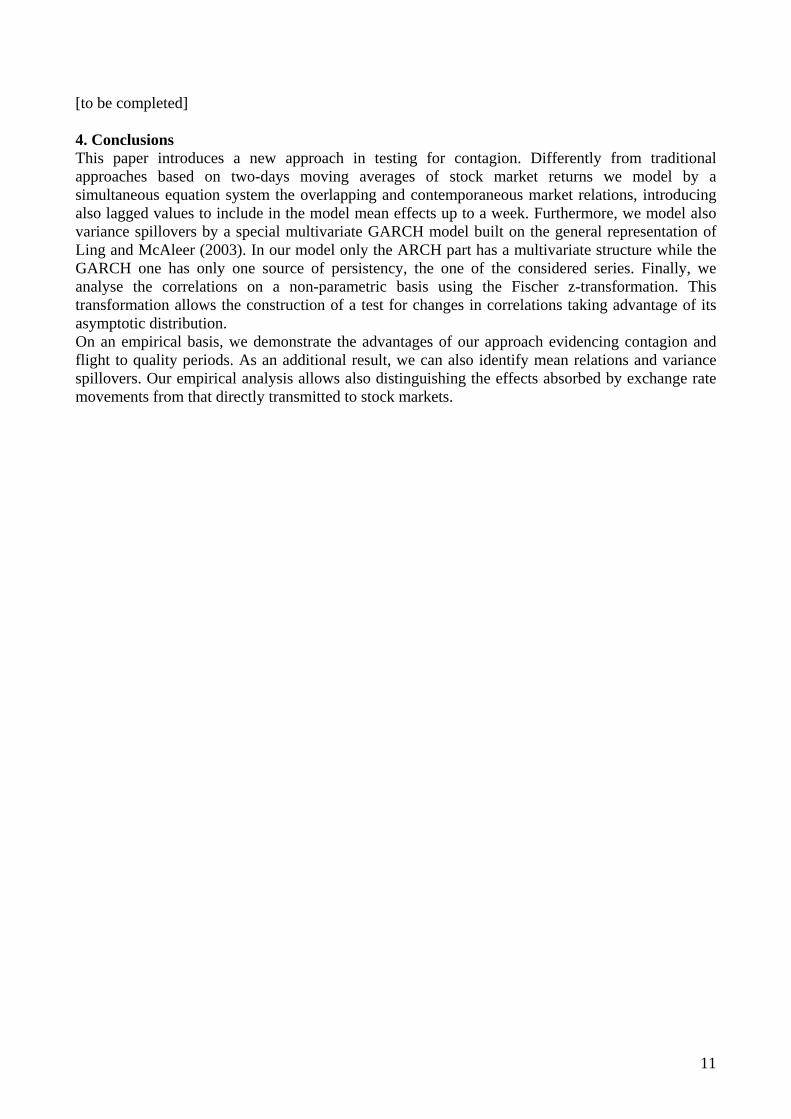
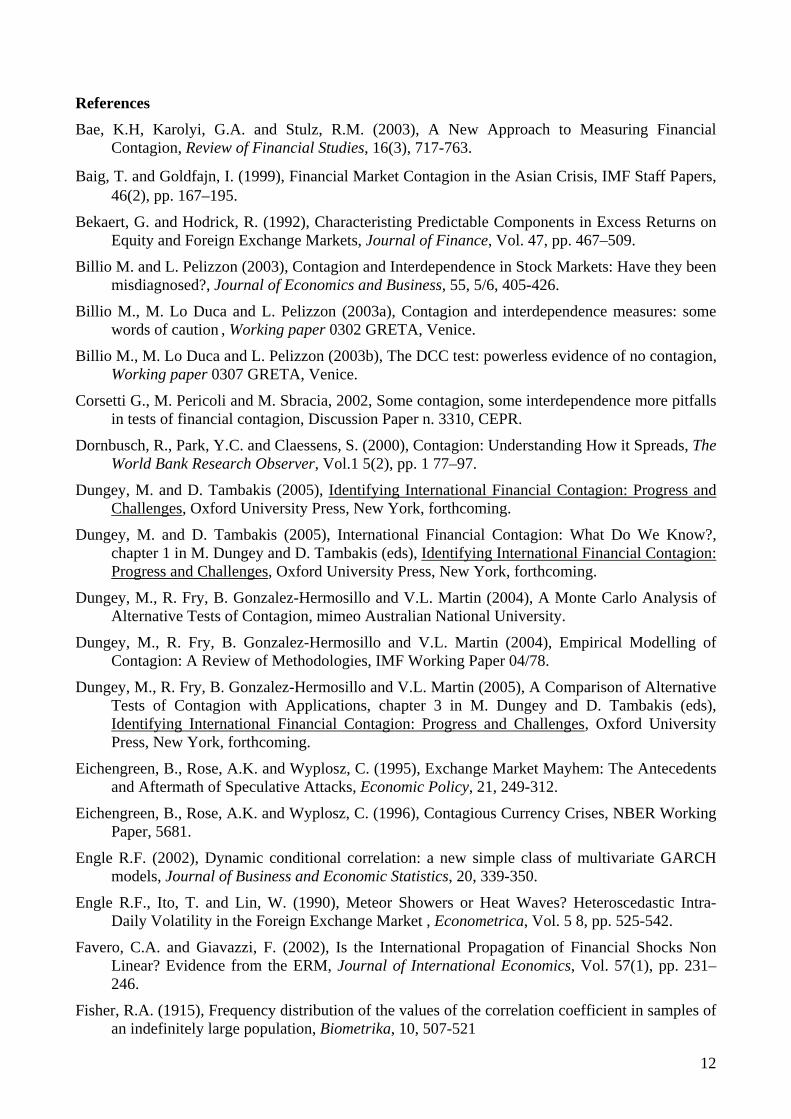
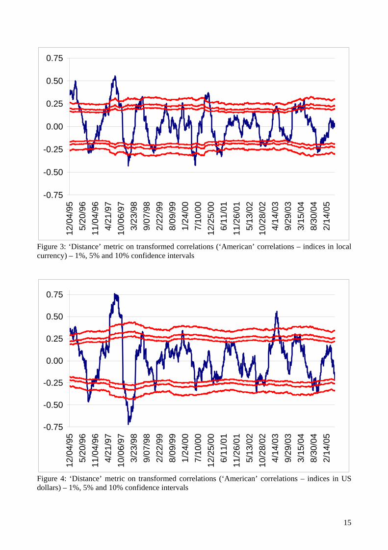
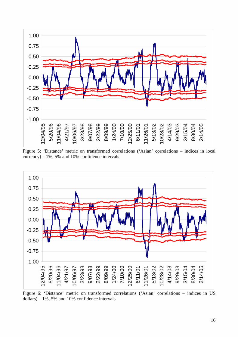
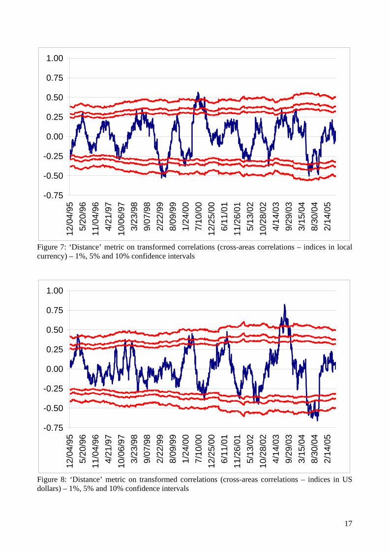
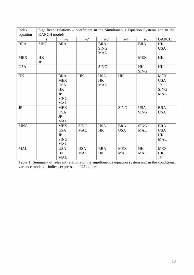
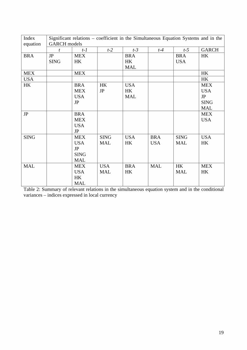
In the empirical analyses we consider two alternative cases: the indices expressed in local currency (that is the original stock market index level) and the indices expressed in a common currency, i.e. US dollars (obtained converting the stock market index level into US dollars). Furthermore, in order to obtained consistent USD-valued stock market indices, the exchange rates have been recorded at the closing of the local market. That is, the exchange rate between the Japan Yen and the US Dollar is recorder at the close of the Japan stock market. By that approach, the exchange rates and the stock market indices are influenced by a common information set. We consider the Asian markets as synchronous even if this is not exactly the case: a preferred approach should be based on stock market indices recorded at a fixed point over the day when all Asian area markets are open. This procedure will avoid any possible problem due to non-synchronous trading. Unfortunately, we have not this type of data and to avoid any possible problem, for the moment, we do not consider any contemporaneous relation within Asian and within American markets. A more detailed analysis is currently under development. We do not report for brevity the tables collecting, for both local currency and US dollar indices cases, the estimated coefficients of the simultaneous equation system and the estimated coefficients of the GARCHX models. These are available from the authors upon request. In all cases, we followed a general to specific modelling strategy by successively imposing several zero restrictions on the general models. The estimated coefficients are all statistically significant even if we have not reported the relevant robust standard errors. The most important results are summarised in the graphs that report the “distance” metric computed on transformed correlations. We considered four different cases: the whole set of available correlations, only the correlations within American markets, only the correlations within Asian markets and the correlations between American and Asian markets. Furthermore, in order to get a more robust identification of relevant correlation movements we report the 1%, 5% and 10% confidence levels. The graphs report both the metric based on local currency indices and the one based on US dollars indices in order to evidence relevant discrepancies. Tables 1 and 2 report all the significant relations. The simultaneous equation system estimates evidence that relevant contemporaneous relations exist between Asian markets and South American markets (for both the cases considered). As expected, the lagged variable coefficients show the impact of US returns on most countries, while other relations appear to exist but no relevant pattern emerges. Finally, a larger number of relevant relations appear when we consider series in US dollars rather than in local currencies. The GARCH estimates point out the existence of spillover effects coming mostly from the US and Hong Kong markets (in most cases and independently on the currency used). We focus now on the correlation ‘distance’ metric graphs reported in Figures 1 to 8. We used a set of indices in US dollars and in local values, therefore we should be able to distinguish if a shock produced contagion effects only on the stock market indices or also in the exchange rates. The exchange rate effects would be included when the analysis is performed on the common currency series (US dollars), which clearly also include movements in the exchange rates. Differently, the series in local currencies evidences movements related only to stock markets adjustments. When the analysis in local currency evidences a change in the correlations (the metric distance test statistics rejects the null hypothesis of equal correlation) while the US dollars series shows no contagion (since the metric distance test statistics accepts the null of equal correlation) it means that the turmoil has been completely offset by exchange rates correlation adjustments. In the end, we can discuss if this would be considered contagion.

10

Differently, when the opposite is true, that is the analysis in local currency does not evidence a change in the correlations which instead appears in the analysis on a common currency, we can also argue if this is an evidence of contagion, since there has been turmoil in the exchange rate market that did not produce effects in the correlations among stock markets. Consequently, only rejections of the null hypothesis that are not offset by the exchange rate market and then propagate to other markets are clear evidences of contagion. These are associated to rejections of the null hypothesis for both the distance metric computed from series in local currency and in US dollars. Our approach can also distinguish between loss of interdependence (an average decrease of correlations) and an increase in stock market linkages (an average increase in the correlations, i.e. contagion strictly speaking). Moreover, by comparing Asian, American and cross-area correlations we can identify areas that originated the shocks. Finally, a comparison within the same window, but on the common currency and on the local currency cases, can be used to test if the exchange rates affect or not the correlation between financial markets. Using this distinction, a preliminary analysis of Figures 1 to 8 evidences the following turbulent periods: i) mid 1996 – a shock originated in Asian markets produced changes in the correlations, which are particularly evident in local currency indices, evidencing that these changes are partially offset by changes in the exchange rates correlations – the most relevant changes occurred in the single-area correlations while the cross-area correlations are limitedly affected (no significant changes detected by evidence of a similar pattern); ii) end 1996 and first half of 1997 – evidence of contagion originated by Asian markets, relevant changes in the correlations in both cases, but mostly on Asian markets – the crisis affected mainly Asian markets (a contagion effect within Asia) – cross-area correlations evidences an increase with blind evidence of contagion – within American indices evidence contagion probably due to the inclusion in the group of emerging market indices (Brasil and Mexico) – the scale differences evidenced by the graphs expressed in local currencies and in US dollars evidence that the financial contagion was partially offset by exchange rate adjustments at least within Asian markets; iii) end 1997 and beginning of 1998 – evidence of loss of interdependence (flight to quality) within Asian and American markets, probably as a consequence of the previous turmoil period, with relevant adjustments in the exchange rate market (the metric is larger when expressed in US dollars); iv) from 2000 to 2001 – evidences of contagion and loss of interdependence – the first associated to the technology market bubble that affected the global financial market, the second is an effect of the 11/9 which induces a flight-to-quality effect – after that some additional evidence of contagion probably associated to a recover/reconstruction of market linkages after the terrorist attack turmoil; v) mid 2003 – evidence of contagion, associated to American markets (Afghanistan effect?) vi) mid 2004 – evidence of loss of interdependence (Iraq effect?).

11

[to be completed] 4. Conclusions This paper introduces a new approach in testing for contagion. Differently from traditional approaches based on two-days moving averages of stock market returns we model by a simultaneous equation system the overlapping and contemporaneous market relations, introducing also lagged values to include in the model mean effects up to a week. Furthermore, we model also variance spillovers by a special multivariate GARCH model built on the general representation of Ling and McAleer (2003). In our model only the ARCH part has a multivariate structure while the GARCH one has only one source of persistency, the one of the considered series. Finally, we analyse the correlations on a non-parametric basis using the Fischer z-transformation. This transformation allows the construction of a test for changes in correlations taking advantage of its asymptotic distribution. On an empirical basis, we demonstrate the advantages of our approach evidencing contagion and flight to quality periods. As an additional result, we can also identify mean relations and variance spillovers. Our empirical analysis allows also distinguishing the effects absorbed by exchange rate movements from that directly transmitted to stock markets.

12

References Bae, K.H, Karolyi, G.A. and Stulz, R.M. (2003), A New Approach to Measuring Financial

Contagion, Review of Financial Studies, 16(3), 717-763.

Baig, T. and Goldfajn, I. (1999), Financial Market Contagion in the Asian Crisis, IMF Staff Papers, 46(2), pp. 167–195.

Bekaert, G. and Hodrick, R. (1992), Characteristing Predictable Components in Excess Returns on Equity and Foreign Exchange Markets, Journal of Finance, Vol. 47, pp. 467–509.

Billio M. and L. Pelizzon (2003), Contagion and Interdependence in Stock Markets: Have they been misdiagnosed?, Journal of Economics and Business, 55, 5/6, 405-426.

Billio M., M. Lo Duca and L. Pelizzon (2003a), Contagion and interdependence measures: some words of caution , Working paper 0302 GRETA, Venice.

Billio M., M. Lo Duca and L. Pelizzon (2003b), The DCC test: powerless evidence of no contagion, Working paper 0307 GRETA, Venice.

Corsetti G., M. Pericoli and M. Sbracia, 2002, Some contagion, some interdependence more pitfalls in tests of financial contagion, Discussion Paper n. 3310, CEPR.

Dornbusch, R., Park, Y.C. and Claessens, S. (2000), Contagion: Understanding How it Spreads, The World Bank Research Observer, Vol.1 5(2), pp. 1 77–97.

Dungey, M. and D. Tambakis (2005), Identifying International Financial Contagion: Progress and Challenges, Oxford University Press, New York, forthcoming.

Dungey, M. and D. Tambakis (2005), International Financial Contagion: What Do We Know?, chapter 1 in M. Dungey and D. Tambakis (eds), Identifying International Financial Contagion: Progress and Challenges, Oxford University Press, New York, forthcoming.

Dungey, M., R. Fry, B. Gonzalez-Hermosillo and V.L. Martin (2004), A Monte Carlo Analysis of Alternative Tests of Contagion, mimeo Australian National University.

Dungey, M., R. Fry, B. Gonzalez-Hermosillo and V.L. Martin (2004), Empirical Modelling of Contagion: A Review of Methodologies, IMF Working Paper 04/78.

Dungey, M., R. Fry, B. Gonzalez-Hermosillo and V.L. Martin (2005), A Comparison of Alternative Tests of Contagion with Applications, chapter 3 in M. Dungey and D. Tambakis (eds), Identifying International Financial Contagion: Progress and Challenges, Oxford University Press, New York, forthcoming.

Eichengreen, B., Rose, A.K. and Wyplosz, C. (1995), Exchange Market Mayhem: The Antecedents and Aftermath of Speculative Attacks, Economic Policy, 21, 249-312.

Eichengreen, B., Rose, A.K. and Wyplosz, C. (1996), Contagious Currency Crises, NBER Working Paper, 5681.

Engle R.F. (2002), Dynamic conditional correlation: a new simple class of multivariate GARCH models, Journal of Business and Economic Statistics, 20, 339-350.

Engle R.F., Ito, T. and Lin, W. (1990), Meteor Showers or Heat Waves? Heteroscedastic Intra-Daily Volatility in the Foreign Exchange Market , Econometrica, Vol. 5 8, pp. 525-542.

Favero, C.A. and Giavazzi, F. (2002), Is the International Propagation of Financial Shocks Non Linear? Evidence from the ERM, Journal of International Economics, Vol. 57(1), pp. 231–246.

Fisher, R.A. (1915), Frequency distribution of the values of the correlation coefficient in samples of an indefinitely large population, Biometrika, 10, 507-521

13

Forbes K. and R. Rigobon (2000), Measuring contagion: conceptual and empirical issues, in S.Claessens and K. Forbes (Eds), International Financial Contagion, Kluwer Academic Publishers.

Forbes K.J. and R. Rigobon (2002), No contagion, only interdependence: measuring stock market comovements, Journal of Finance, 57/5, 2223-2261.

Glick, R. and Rose, A.K. (1999), Contagion and Trade: Why are Currency Crises Regional?, Journal of International Money and Finance, 18(4), 603-17.

Grubel, H.G. and Fadner R. (1971), The Interdependence of International Equity Markets, Journal of Finance, Vol. 26, pp. 89–94.

Kaminsky, G.L. and Reinhart, C.M. (2000), On Crises, Contagion and Confusion, Journal of International Economics, 51(1), 145-168.

King, M. and Wadhwani, S. (1990), Transmission of Volatility Between Stock Markets, Review of Financial Studies, Vol. 3 (1), pp. 5– 33.

Ling, S. and M. McAleer (2003), Asymptotic theory for a vector ARMA-GARCH model, Econometric Theory, 19, 278-308.

Pesaran, H. and Pick, A. (2004), Econometric Issues in the Analysis of Contagion, CESifo Working Paper No. 1176.

Pritsker, M. (2002), Large Investors and Liquidity: A Review of the Literature, in Committee on the Global Financial System (ed), Risk Measurement and Systemic Risk, Proceedings of the Third Joint Central Bank Research Conference.

Rao, D.C. (1979), Joint distribution of z-tranformations estimated from the same sample, Human Heredity, 29, 334-336

Rigobon R. (2001), Contagion: how to measure it?, NBER Working Paper No. w8118.

Scheffé, H. (1970), Practical solutions to the Behrens-Fisher Problem, Journal of the American Statistical Association, 65, 1501-1508

Sharpe, W. (1964), Capital Asset Prices: A Theory of Market Equilibrium Under Conditions of Risk, Journal of Finance, Vol. 19, pp. 425–42.

14

-1.50-1.25-1.00-0.75-0.50-0.250.000.250.500.751.001.251.50

12/0

4/95

5/20

/96

11/0

4/96

4/21

/97

10/0

6/97

3/23

/98

9/07

/98

2/22

/99

8/09

/99

1/24

/00

7/10

/00

12/2

5/00

6/11

/01

11/2

6/01

5/13

/02

10/2

8/02

4/14

/03

9/29

/03

3/15

/04

8/30

/04

2/14

/05

Figure 1: ‘Distance’ metric on transformed correlations (full set of correlations – indices in local currency) –1%, 5% and 10% confidence intervals

-1.50-1.25-1.00-0.75-0.50-0.250.000.250.500.751.001.251.50

12/0

4/95

5/20

/96

11/0

4/96

4/21

/97

10/0

6/97

3/23

/98

9/07

/98

2/22

/99

8/09

/99

1/24

/00

7/10

/00

12/2

5/00

6/11

/01

11/2

6/01

5/13

/02

10/2

8/02

4/14

/03

9/29

/03

3/15

/04

8/30

/04

2/14

/05

Figure 2: ‘Distance’ metric on transformed correlations (full set of correlations – indices in US dollars) – 1%, 5% and 10% confidence intervals

15

-0.75

-0.50

-0.25

0.00

0.25

0.50

0.7512

/04/

955/

20/9

611

/04/

964/

21/9

710

/06/

973/

23/9

89/

07/9

82/

22/9

98/

09/9

91/

24/0

07/

10/0

012

/25/

006/

11/0

111

/26/

015/

13/0

210

/28/

024/

14/0

39/

29/0

33/

15/0

48/

30/0

42/

14/0

5

Figure 3: ‘Distance’ metric on transformed correlations (‘American’ correlations – indices in local currency) – 1%, 5% and 10% confidence intervals

-0.75

-0.50

-0.25

0.00

0.25

0.50

0.75

12/0

4/95

5/20

/96

11/0

4/96

4/21

/97

10/0

6/97

3/23

/98

9/07

/98

2/22

/99

8/09

/99

1/24

/00

7/10

/00

12/2

5/00

6/11

/01

11/2

6/01

5/13

/02

10/2

8/02

4/14

/03

9/29

/03

3/15

/04

8/30

/04

2/14

/05

Figure 4: ‘Distance’ metric on transformed correlations (‘American’ correlations – indices in US dollars) – 1%, 5% and 10% confidence intervals

16

-1.00

-0.75

-0.50

-0.25

0.00

0.25

0.50

0.75

1.0012

/04/

955/

20/9

611

/04/

964/

21/9

710

/06/

973/

23/9

89/

07/9

82/

22/9

98/

09/9

91/

24/0

07/

10/0

012

/25/

006/

11/0

111

/26/

015/

13/0

210

/28/

024/

14/0

39/

29/0

33/

15/0

48/

30/0

42/

14/0

5

Figure 5: ‘Distance’ metric on transformed correlations (‘Asian’ correlations – indices in local currency) – 1%, 5% and 10% confidence intervals

-1.00

-0.75

-0.50

-0.25

0.00

0.25

0.50

0.75

1.00

12/0

4/95

5/20

/96

11/0

4/96

4/21

/97

10/0

6/97

3/23

/98

9/07

/98

2/22

/99

8/09

/99

1/24

/00

7/10

/00

12/2

5/00

6/11

/01

11/2

6/01

5/13

/02

10/2

8/02

4/14

/03

9/29

/03

3/15

/04

8/30

/04

2/14

/05

Figure 6: ‘Distance’ metric on transformed correlations (‘Asian’ correlations – indices in US dollars) – 1%, 5% and 10% confidence intervals

17

-0.75

-0.50

-0.25

0.00

0.25

0.50

0.75

1.0012

/04/

955/

20/9

611

/04/

964/

21/9

710

/06/

973/

23/9

89/

07/9

82/

22/9

98/

09/9

91/

24/0

07/

10/0

012

/25/

006/

11/0

111

/26/

015/

13/0

210

/28/

024/

14/0

39/

29/0

33/

15/0

48/

30/0

42/

14/0

5

Figure 7: ‘Distance’ metric on transformed correlations (cross-areas correlations – indices in local currency) – 1%, 5% and 10% confidence intervals

-0.75

-0.50

-0.25

0.00

0.25

0.50

0.75

1.00

12/0

4/95

5/20

/96

11/0

4/96

4/21

/97

10/0

6/97

3/23

/98

9/07

/98

2/22

/99

8/09

/99

1/24

/00

7/10

/00

12/2

5/00

6/11

/01

11/2

6/01

5/13

/02

10/2

8/02

4/14

/03

9/29

/03

3/15

/04

8/30

/04

2/14

/05

Figure 8: ‘Distance’ metric on transformed correlations (cross-areas correlations – indices in US dollars) – 1%, 5% and 10% confidence intervals

18

Significant relations – coefficient in the Simultaneous Equation Systems and in the GARCH models

Index equation

t t-1 t-2 t-3 t-4 t-5 GARCH BRA SING BRA BRA

SING MAL

BRA HK USA

MEX HK JP

MEX HK

USA SING HK SING

HK

HK BRA MEX USA HK JP SING MAL

HK USA HK MAL

HK MEX USA JP SING MAL

JP MEX USA JP MAL

SING USA SING

BRA USA

SING MEX USA JP SING MAL

SING MAL

USA HK

BRA USA

SING MAL

BRA USA HK MAL

MAL USA HK MAL

USA MAL

BRA HK

MEX MAL

HK MAL

MEX HK JP

Table 1: Summary of relevant relations in the simultaneous equation system and in the conditional variance models – indices expressed in US dollars

19

Significant relations – coefficient in the Simultaneous Equation Systems and in the GARCH models

Index equation

t t-1 t-2 t-3 t-4 t-5 GARCH BRA JP

SING MEX HK

BRA HK MAL

BRA USA

HK

MEX MEX HK USA HK HK BRA

MEX USA JP

HK JP

USA HK MAL

MEX USA JP SING MAL

JP BRA MEX USA JP

MEX USA

SING MEX USA JP SING MAL

SING MAL

USA HK

BRA USA

SING MAL

USA HK

MAL MEX USA HK MAL

USA MAL

BRA HK

MAL HK MAL

MEX HK

Table 2: Summary of relevant relations in the simultaneous equation system and in the conditional variances – indices expressed in local currency