market market-driven dynamic transmission expansion planning … · market-driven dynamic...
TRANSCRIPT
Market-driven dynamic transmission expansion planning 1
Market-driven dynamic transmission expansion planning
MarketMarket--driven dynamic transmission driven dynamic transmission expansion planningexpansion planning
Ing. Álvaro Martínez Valle (UMA)Dr. José Antonio Aguado Sánchez (UMA)
Dr. Sebastián de la Torre Fazio (UMA)Dr. Javier Contreras Sanz (UCLM)
Ing. Álvaro Martínez Valle (UMA)Dr. José Antonio Aguado Sánchez (UMA)
Dr. Sebastián de la Torre Fazio (UMA)Dr. Javier Contreras Sanz (UCLM)
ESCUELA TÉCNICA SUPERIOR DE INGENIEROS INDUSTRIALESUNIVERSIDAD DE CASTILLA – LA MANCHA
13071 Ciudad Real, Spain
ESCUELA TÉCNICA SUPERIOR DE INGENIEROS INDUSTRIALESUNIVERSIDAD DE MÁLAGA
29071 Málaga, Spain
Market-driven dynamic transmission expansion planning 2
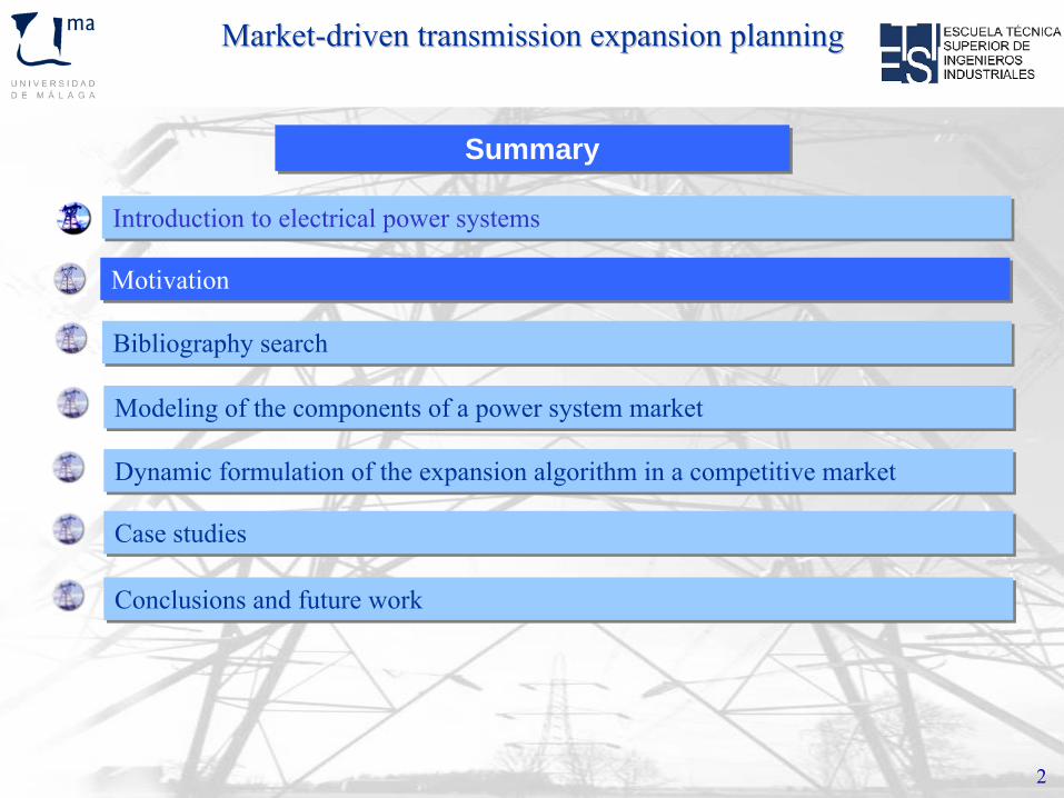
MarketMarket--driven transmission expansion planningdriven transmission expansion planning
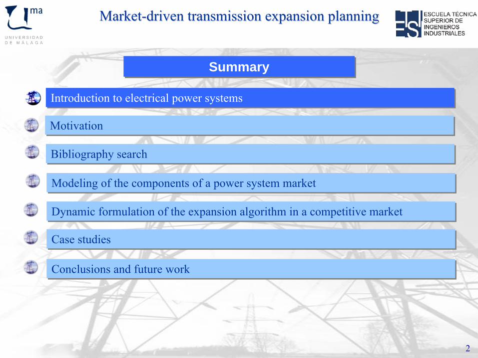
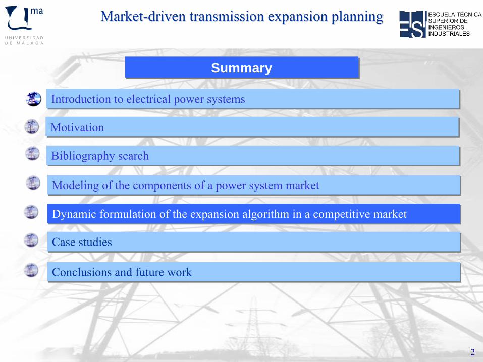
SummarySummary
Introduction to electrical power systemsIntroduction to electrical power systems
MotivationMotivation
Bibliography searchBibliography search
Dynamic formulation of the expansion algorithm in a competitive marketDynamic formulation of the expansion algorithm in a competitive market
Case studiesCase studies
Conclusions and future workConclusions and future work
2
Modeling of the components of a power system marketModeling of the components of a power system market
Market-driven dynamic transmission expansion planning 3
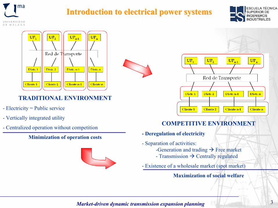
Introduction to electrical power systemsIntroduction to electrical power systems
TRADITIONAL ENVIRONMENT-
Electricity = Public service
- Vertically integrated utility
- Centralized operation without competition
Minimization of operation costs
COMPETITIVE ENVIRONMENT-
Deregulation of electricity
- Separation of activities:-Generation and trading Free market- Transmission Centrally regulated
- Existence of a wholesale market (spot market)
Maximization of social welfare
Market-driven dynamic transmission expansion planning 4
MarketMarket--driven transmission expansion planningdriven transmission expansion planning
SummarySummary
Introduction to electrical power systemsIntroduction to electrical power systems
MotivationMotivation
Bibliography searchBibliography search
Dynamic formulation of the expansion algorithm in a competitive marketDynamic formulation of the expansion algorithm in a competitive market
Case studiesCase studies
Conclusions and future workConclusions and future work
2
Modeling of the components of a power system marketModeling of the components of a power system market
Market-driven dynamic transmission expansion planning 5
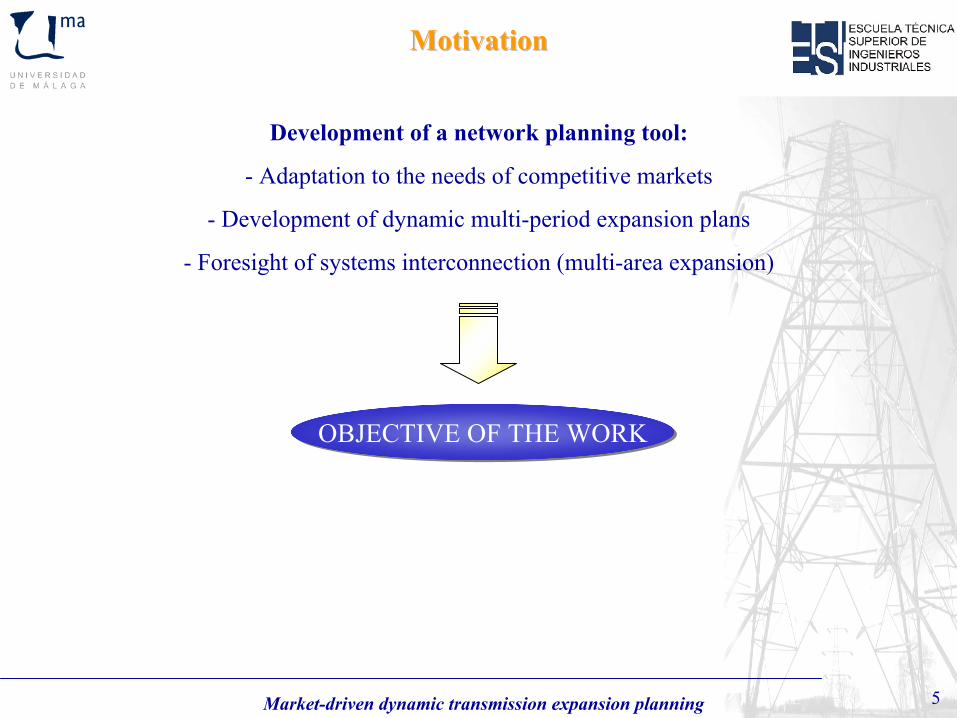
MotivationMotivation
OBJECTIVE OF THE WORK
Development of a network planning tool:
- Adaptation to the needs of competitive markets
- Development of dynamic multi-period expansion plans
- Foresight of systems interconnection (multi-area expansion)
Market-driven dynamic transmission expansion planning 6
MarketMarket--driven transmission expansion planningdriven transmission expansion planning
SummarySummary
Introduction to electrical power systemsIntroduction to electrical power systems
MotivationMotivation
Bibliography searchBibliography search
Dynamic formulation of the expansion algorithm in a competitive marketDynamic formulation of the expansion algorithm in a competitive market
Case studiesCase studies
Conclusions and future workConclusions and future work
2
Modeling of the components of a power system marketModeling of the components of a power system market
Market-driven dynamic transmission expansion planning 7
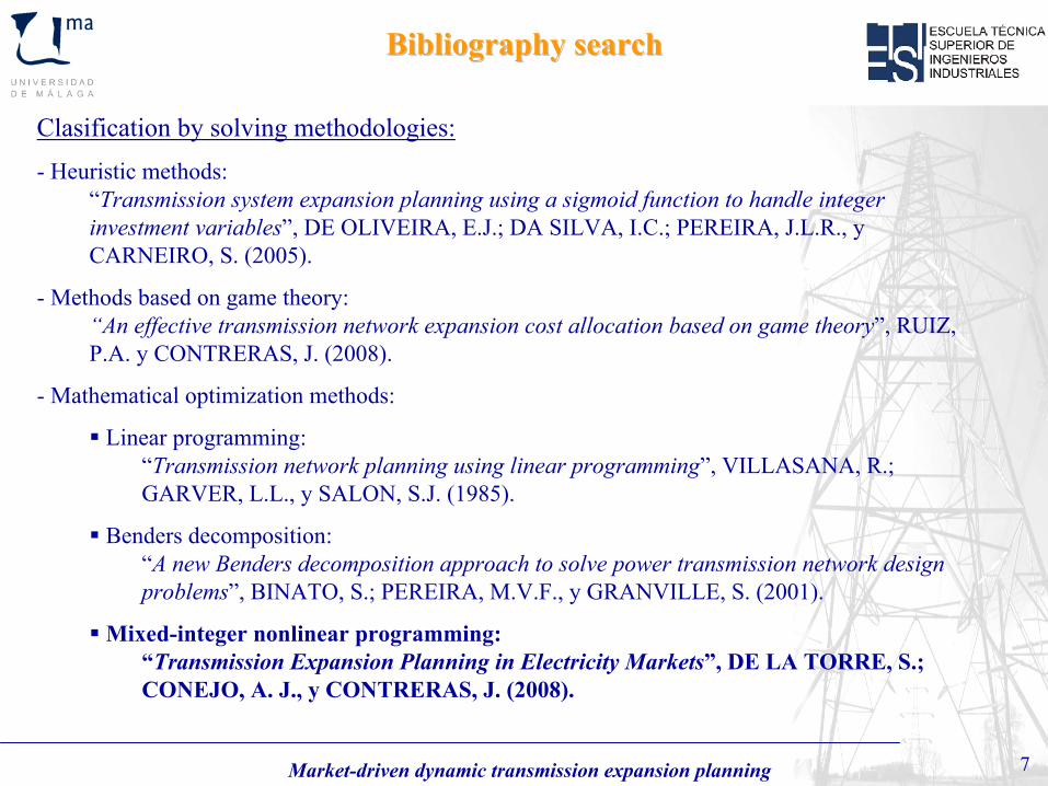
Bibliography searchBibliography search
Clasification by solving methodologies:- Heuristic methods:
“Transmission system expansion planning using a sigmoid function to handle integer investment variables”, DE OLIVEIRA, E.J.; DA SILVA, I.C.; PEREIRA, J.L.R., y CARNEIRO, S. (2005).
- Methods based on game theory:“An effective transmission network expansion cost allocation based on game theory”, RUIZ, P.A. y CONTRERAS, J. (2008).
- Mathematical optimization methods:
Linear programming:“Transmission network planning using linear programming”, VILLASANA, R.; GARVER, L.L., y SALON, S.J. (1985).
Benders decomposition:“A new Benders decomposition approach to solve power transmission
network design problems”, BINATO, S.; PEREIRA, M.V.F., y GRANVILLE, S. (2001).
Mixed-integer nonlinear programming:“Transmission Expansion Planning in Electricity Markets”, DE LA TORRE, S.; CONEJO, A. J., y CONTRERAS, J. (2008).
Market-driven dynamic transmission expansion planning 8
MarketMarket--driven transmission expansion planningdriven transmission expansion planning
SummarySummary
Introduction to electrical power systemsIntroduction to electrical power systems
MotivationMotivation
Bibliography searchBibliography search
Dynamic formulation of the expansion algorithm in a competitive marketDynamic formulation of the expansion algorithm in a competitive market
Case studiesCase studies
Conclusions and future workConclusions and future work
2
Modeling of the components of a power system marketModeling of the components of a power system market
Market-driven dynamic transmission expansion planning 9
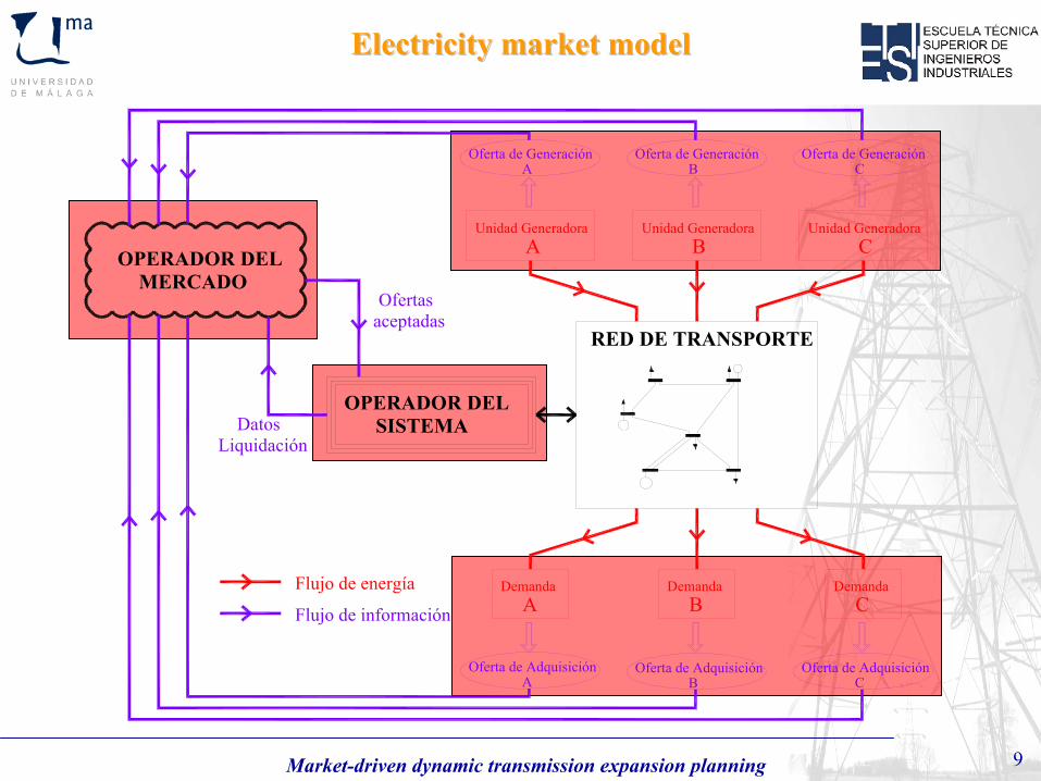
Unidad Generadora A
Oferta de Generación A
RED DE TRANSPORTE
Unidad Generadora B
Unidad Generadora C
Demanda A
Demanda B
Demanda C
OPERADOR DEL MERCADO
OPERADOR DEL SISTEMA
Flujo de energía
Flujo de información
Ofertas aceptadas
Datos Liquidación
Oferta de Generación B
Oferta de Generación C
Oferta de Adquisición B
Oferta de Adquisición A
Oferta de Adquisición C
Electricity market modelElectricity market model
Market-driven dynamic transmission expansion planning 10
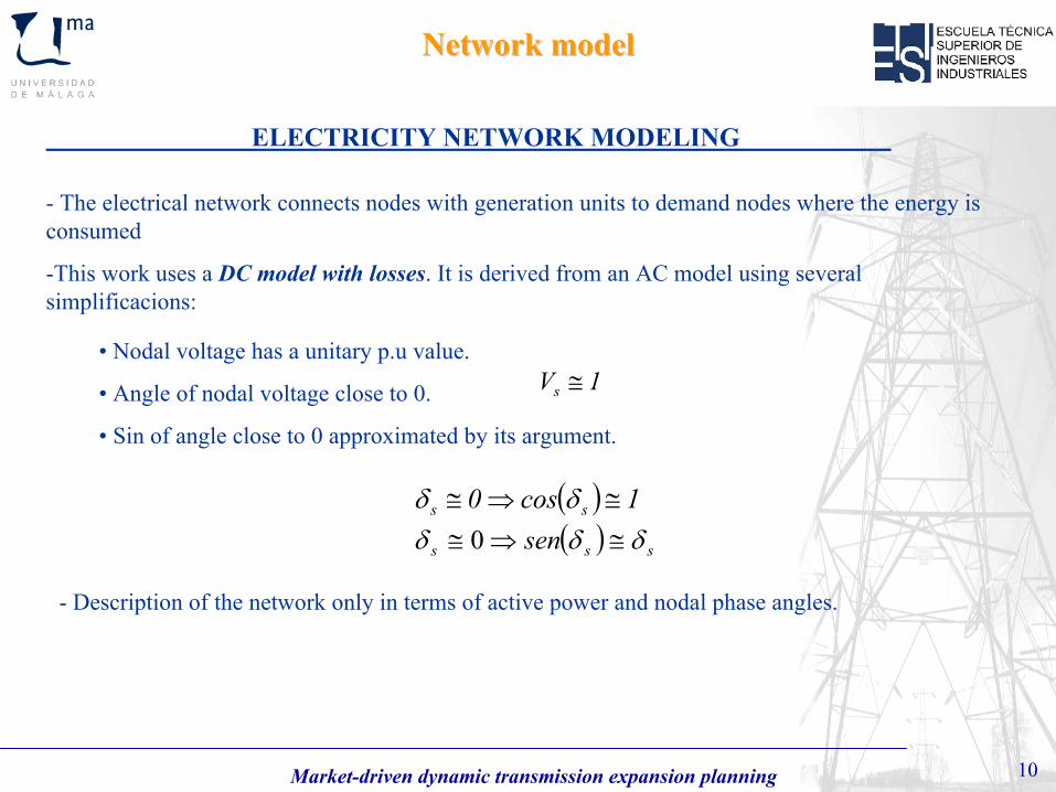
ELECTRICITY NETWORK MODELING
-
The electrical network connects nodes with generation units to demand nodes where the energy is consumed
-This work uses a DC model with losses. It is derived from an AC model using several simplificacions:
• Nodal voltage has a unitary p.u value.
• Angle of nodal voltage close to 0.
• Sin of angle close to 0 approximated by its argument.
( ) 1cos0 ss ≅⇒≅ δδ( ) sss sen δδδ ≅⇒≅ 0
-
Description of the network only in terms of active power and nodal phase angles.
Network modelNetwork model
1Vs ≅
Market-driven dynamic transmission expansion planning 11
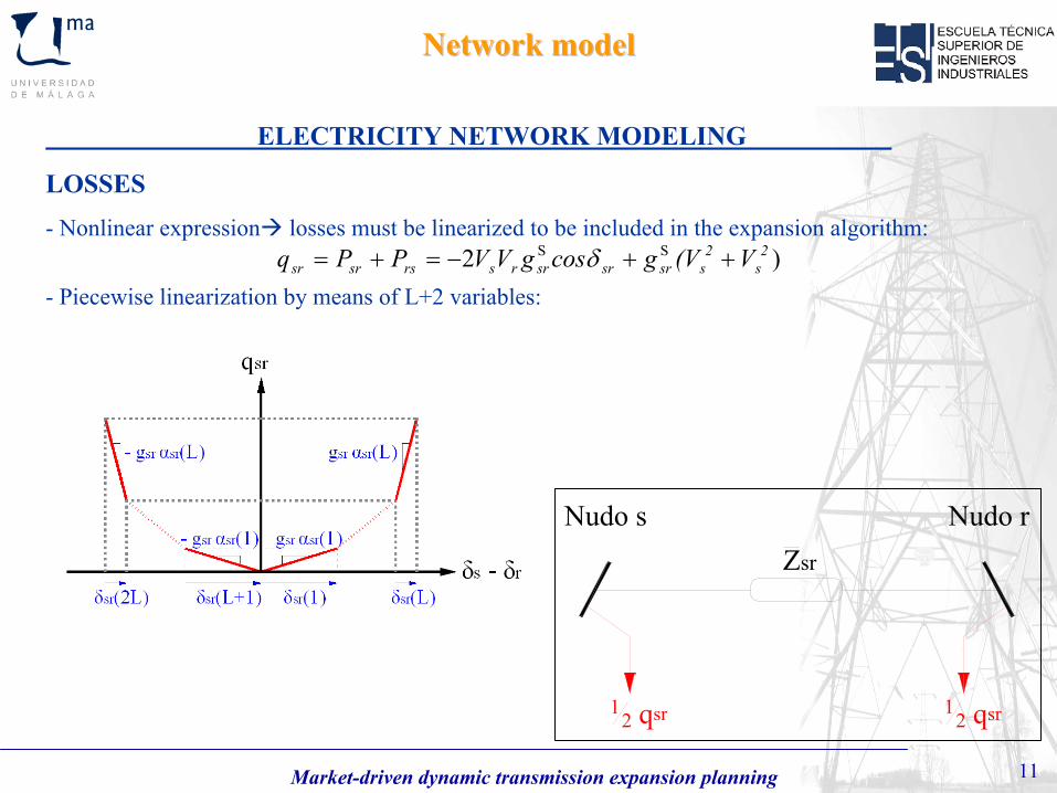
ELECTRICITY NETWORK MODELING
LOSSES- Nonlinear expression losses must be linearized to be included in the expansion algorithm:
-
Piecewise linearization by means of L+2 variables:)2 SS 2
s2
ssrsrsrrsrssrsr V(VgcosgVVPPq ++−=+= δ
Network modelNetwork model
Nudo s Nudo r Zsr
12 qsr1
2 qsr
Market-driven dynamic transmission expansion planning 12
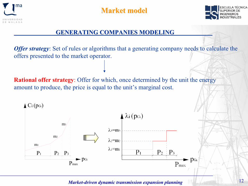
GENERATING COMPANIES MODELINGGENERATING COMPANIES MODELING
Offer strategy: Set of rules or algorithms that a generating company needs to calculate the offers
presented to the market operator.
Rational offer strategy:
Offer for which, once determined by the unit the energy amount to produce, the price is equal to the unit’s marginal cost.
pGi
P3P2P1
m3
m2
m1
Ci (pGi)
Pmax
Market modelMarket model
Market-driven dynamic transmission expansion planning 13
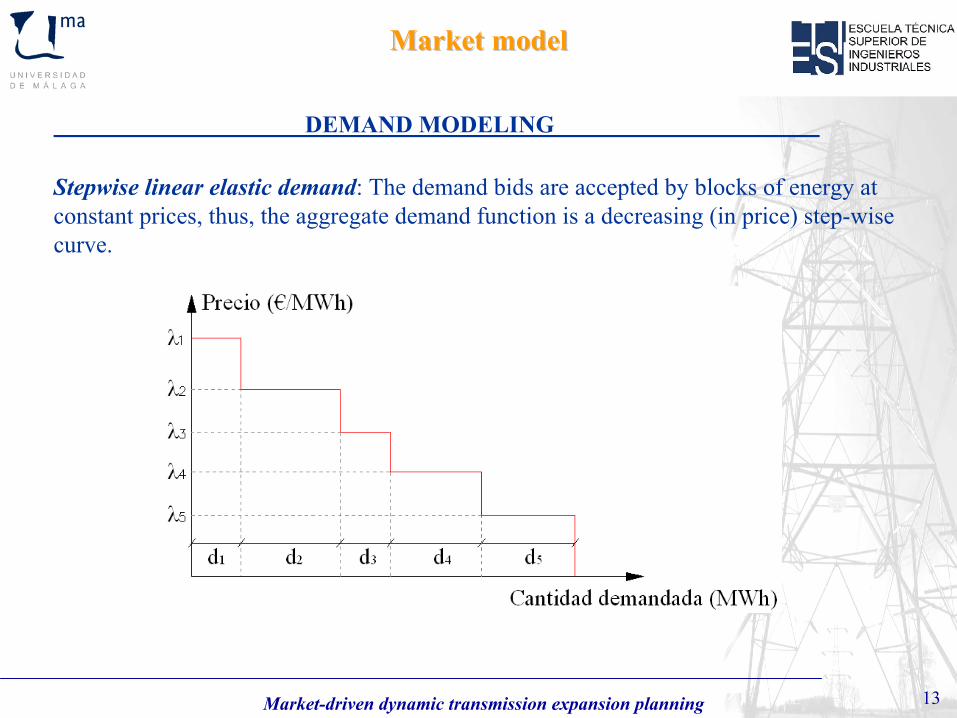
DEMAND MODELING
Stepwise linear elastic demand: The demand bids are accepted by blocks of energy at constant prices, thus, the aggregate demand function is a decreasing (in price)
step-wise
curve.
Market modelMarket model
Market-driven dynamic transmission expansion planning 14
MARKET MATCHING MODELING
In a deregulated system, the price of electricity is composed of
two terms:
- One term is related to the cost of generation.
- The other term is related to the transmission cost.
Nodal prices or Locational Marginal Prices (LMPs):
•
LMPs represent a market mechanism whose value is a function of the node placement in the network.
• LMPs reflect the marginal costs in time and space.
•
LMPs are obtained as dual variables (Lagrange multipliers) associated with the balance equations of an optimal power flow (OPF).
Market modelMarket model
Market-driven dynamic transmission expansion planning 15
MarketMarket--driven transmission expansion planningdriven transmission expansion planning
SummarySummary
Introduction to electrical power systemsIntroduction to electrical power systems
MotivationMotivation
Bibliography searchBibliography search
Dynamic formulation of the expansion algorithm in a competitive marketDynamic formulation of the expansion algorithm in a competitive market
Case studiesCase studies
Conclusions and future workConclusions and future work
2
Modeling of the components of a power system marketModeling of the components of a power system market
Market-driven dynamic transmission expansion planning 16
1)r1()r1(r
t
t
−++⋅
=τ8761000
=σ
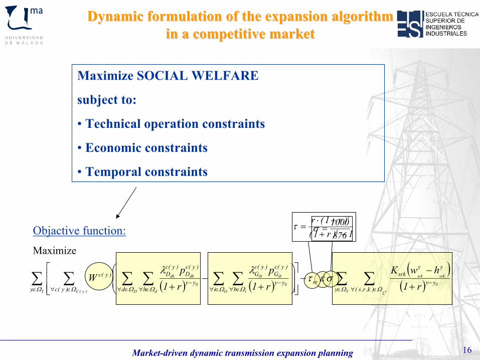
Maximize SOCIAL WELFARE
subject to:
• Technical operation constraints
• Economic constraints
• Temporal constraints
Objactive function:Maximize
( ) ( )( )
( )∑ ∑ ∑∑ ∑ ∑∑ ∑∈ ∈ ∈∀
−∈∀ ∈∀ ∈∀
−∈∀ ∈∀
−+
+
−−
⎥⎥⎦
⎤
⎢⎢⎣
⎡⎟⎟⎠
⎞⎜⎜⎝
⎛
+−
+Y Y L
0
srksrk
)y(C G i0
ibib
D d0
dhdh
y y )k,r,s(yy
yysrk
sr)y(c i b
yy
)y(cG
)y(cG
d hyy
)y(cD
)y(cD)y(c
r1hwK
r1p
r1p
WΩ Ω ΩΩ Ω ΩΩ Ω
σετλλ
Dynamic formulation of the expansion algorithm Dynamic formulation of the expansion algorithm in a competitive marketin a competitive market
Market-driven dynamic transmission expansion planning 17
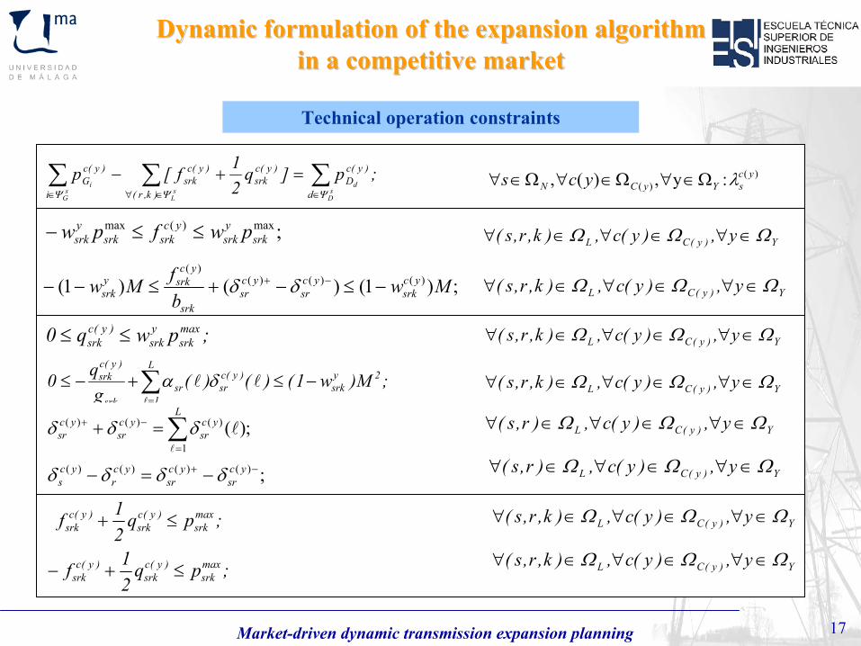
Balance de potencia
Flujos de potencia sin pérdidas
Linealización de las pérdidas
Flujos de potencia máximos
Technical operation constraints
Dynamic formulation of the expansion algorithm Dynamic formulation of the expansion algorithm in a competitive marketin a competitive market
;p]q21f[p
sD
ds
Ls
G
id
)y(cD
)y(csrk
)k,r(
)y(csrk
i
)y(cG ∑∑∑
∈∈∀∈
=+−ΨΨΨ
)()( :y,)(, yc
sYyCN ycs λΩ∈∀Ω∈∀Ω∈∀
;max)(maxsrk
ysrk
ycsrksrk
ysrk pwfpw ≤≤−
;)1()()1( )()()()(
MwbfMw yc
srkyc
sryc
srsrk
ycsrky
srk −≤−+≤−− −+ δδ
Y)y(CL y,)y(c,)k,r,s( ΩΩΩ ∈∀∈∀∈∀
Y)y(CL y,)y(c,)k,r,s( ΩΩΩ ∈∀∈∀∈∀
;pwq0 maxsrk
ysrk
)y(csrk ≤≤
;M)w1()()(g
q0 2ysrk
)y(csr
L
1sr
srk
)y(csrk −≤+−≤ ∑
=
lll
δα
;)(1
)()()( ∑=
−+ =+L
ycsr
ycsr
ycsr
l
lδδδ
;)()()()( −+ −=− ycsr
ycsr
ycr
ycs δδδδ
Y)y(CL y,)y(c,)k,r,s( ΩΩΩ ∈∀∈∀∈∀
Y)y(CL y,)y(c,)k,r,s( ΩΩΩ ∈∀∈∀∈∀
Y)y(CL y,)y(c,)r,s( ΩΩΩ ∈∀∈∀∈∀
Y)y(CL y,)y(c,)r,s( ΩΩΩ ∈∀∈∀∈∀
;pq21f max
srk)y(c
srk)y(c
srk ≤+
;pq21f max
srk)y(c
srk)y(c
srk ≤+−
Y)y(CL y,)y(c,)k,r,s( ΩΩΩ ∈∀∈∀∈∀
Y)y(CL y,)y(c,)k,r,s( ΩΩΩ ∈∀∈∀∈∀
Market-driven dynamic transmission expansion planning 18
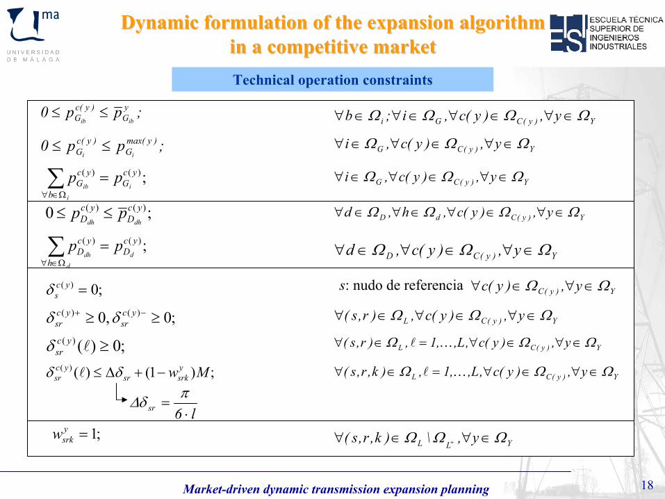
Technical operation constraints
Dynamic formulation of the expansion algorithm Dynamic formulation of the expansion algorithm in a competitive marketin a competitive market
Máxima potencia generada ofertada
Máxima potencia de demanda ofertada
Límites para las variables de fase
Fijación de variables para líneas existentes
;pp0 yG
)y(cG ibib
≤≤
;pp0 )ymax(G
)y(cG ii
≤≤
;)()( ycG
b
ycG i
i
ibpp =∑
Ω∈∀
Y)y(CGi y,)y(c,i;b ΩΩΩΩ ∈∀∈∀∈∀∈∀
Y)y(CG y,)y(c,i ΩΩΩ ∈∀∈∀∈∀
Y)y(CG y,)y(c,i ΩΩΩ ∈∀∈∀∈∀
;0 )()( ycD
ycD dhdh
pp ≤≤
;)()( ycD
h
ycD d
d
dhpp =∑
Ω∈∀
Y)y(CdD y,)y(c,h,d ΩΩΩΩ ∈∀∈∀∈∀∈∀
Y)y(CD y,)y(c,d ΩΩΩ ∈∀∈∀∈∀
;0)( =ycsδ
;0 ,0 )()( ≥≥ −+ ycsr
ycsr δδ
;0)()( ≥lycsrδ
;)1()()( Mwysrksr
ycsr −+Δ≤ δδ l
Y)y(C y,)y(c ΩΩ ∈∀∈∀s: nudo de referencia
Y)y(CL y,)y(c,)r,s( ΩΩΩ ∈∀∈∀∈∀
Y)y(CL y,)y(c,,L,1 ,)r,s( ΩΩΩ ∈∀∈∀=∈∀ Kl
Y)y(CL y,)y(c,,L,1,)k,r,s( ΩΩΩ ∈∀∈∀=∈∀ Kl
l6sr ⋅=
πδΔ
;1=ysrkw
YLL y,\)k,r,s( ΩΩΩ ∈∀∈∀ +
Market-driven dynamic transmission expansion planning 19
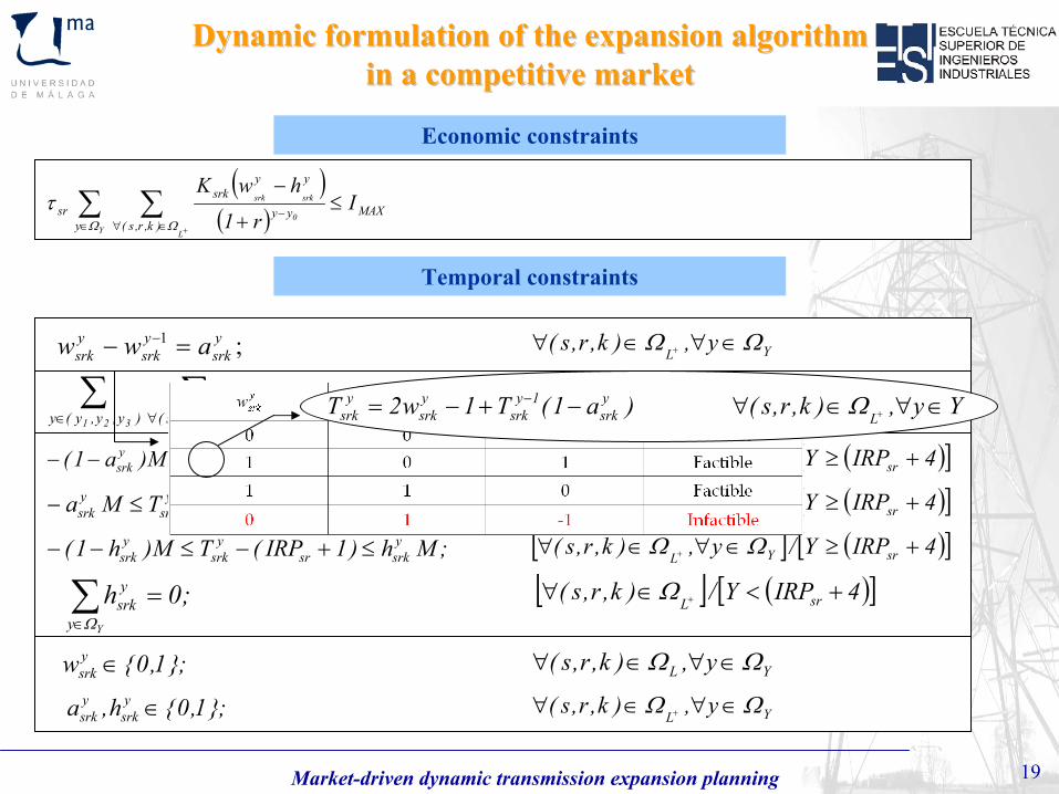
Economic constraints
Dynamic formulation of the expansion algorithm Dynamic formulation of the expansion algorithm in a competitive marketin a competitive market
Límite de inversión
Temporal constraints
Relación lógica
NO construcción en los 3 primeros años
Definición de la variable de amortización
Definición de variables binarias
( )( ) MAX
y )k,r,s(yy
yysrk
sr Ir1
hwK
Y L
0
srksrk ≤+
−∑ ∑∈ ∈∀
−+Ω Ω
τ
;1 ysrk
ysrk
ysrk aww =− −
YLy,)k,r,s( ΩΩ ∈∀∈∀ +
;0w)y,y,y(y )k,r,s(
ysrk
321 L
=∑ ∑∈ ∈∀ +Ω
};1,0{h,a ysrk
ysrk ∈ YL
y,)k,r,s( ΩΩ ∈∀∈∀ +
};1,0{wysrk ∈ YL y,)k,r,s( ΩΩ ∈∀∈∀
;MaT1w2TMa ysrk
1ysrk
ysrk
ysrk
ysrk ≤−+−≤− −
;M)a1(1w2TM)a1( ysrk
ysrk
ysrk
ysrk −≤+−≤−−
;Mh)1IRP(TM)h1( ysrksr
ysrk
ysrk ≤+−≤−−
;0hYy
ysrk =∑
∈Ω
[ ] ( )[ ]4IRPY/y,)k,r,s( srYL +≥∈∀∈∀ + ΩΩ
[ ] ( )[ ]4IRPY/y,)k,r,s( srYL +≥∈∀∈∀ + ΩΩ
[ ] ( )[ ]4IRPY/y,)k,r,s( srYL +≥∈∀∈∀ + ΩΩ
[ ] ( )[ ]4IRPY/)k,r,s( srL+<∈∀ +Ω
Yy,)k,r,s()a1(T1w2T Lysrk
1ysrk
ysrk
ysrk ∈∀∈∀−+−= +
− Ω
Market-driven dynamic transmission expansion planning 20
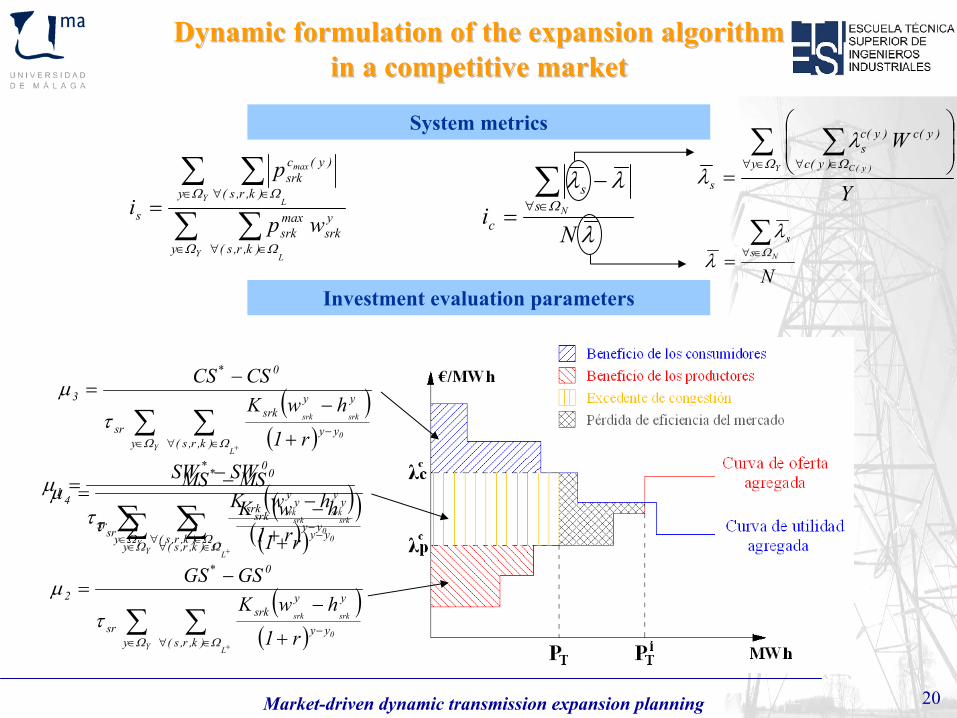
System metrics
∑ ∑
∑ ∑
∈ ∈∀
∈ ∈∀=
Y L
Y L
max
y )k,r,s(
ysrk
maxsrk
y )k,r,s(
)y(csrk
s wp
p
i
Ω Ω
Ω Ω
λ
λλΩ
Ni Ns
s
c
∑∈∀
−=
Y
WY )y(Cy )y(c
)y(c)y(cs
s
∑ ∑∈∀ ∈∀
⎟⎟⎠
⎞⎜⎜⎝
⎛
=Ω Ω
λ
λ
NNs
s∑∈∀= Ω
λλ
Investment evaluation parameters
( )( )∑ ∑
∈ ∈∀−
+ +
−−
=
Y L
0
srksrk
y )k,r,s(yy
yysrk
sr
0*
1
r1
hwKSWSW
Ω Ω
τμ
Dynamic formulation of the expansion algorithm Dynamic formulation of the expansion algorithm in a competitive marketin a competitive market
( )( )∑ ∑
∈ ∈∀−
+ +
−−
=
Y L
0
srksrk
y )k,r,s(yy
yysrk
sr
0*
3
r1
hwKCSCS
Ω Ω
τμ
( )( )∑ ∑
∈ ∈∀−
+ +
−−
=
Y L
0
srksrk
y )k,r,s(yy
yysrk
sr
0*
2
r1
hwKGSGS
Ω Ω
τμ
( )( )∑ ∑
∈ ∈∀−
+ +
−−
=
Y L
0
srksrk
y )k,r,s(yy
yysrk
sr
0*
4
r1
hwKMSMS
Ω Ω
τμ
Market-driven dynamic transmission expansion planning 21
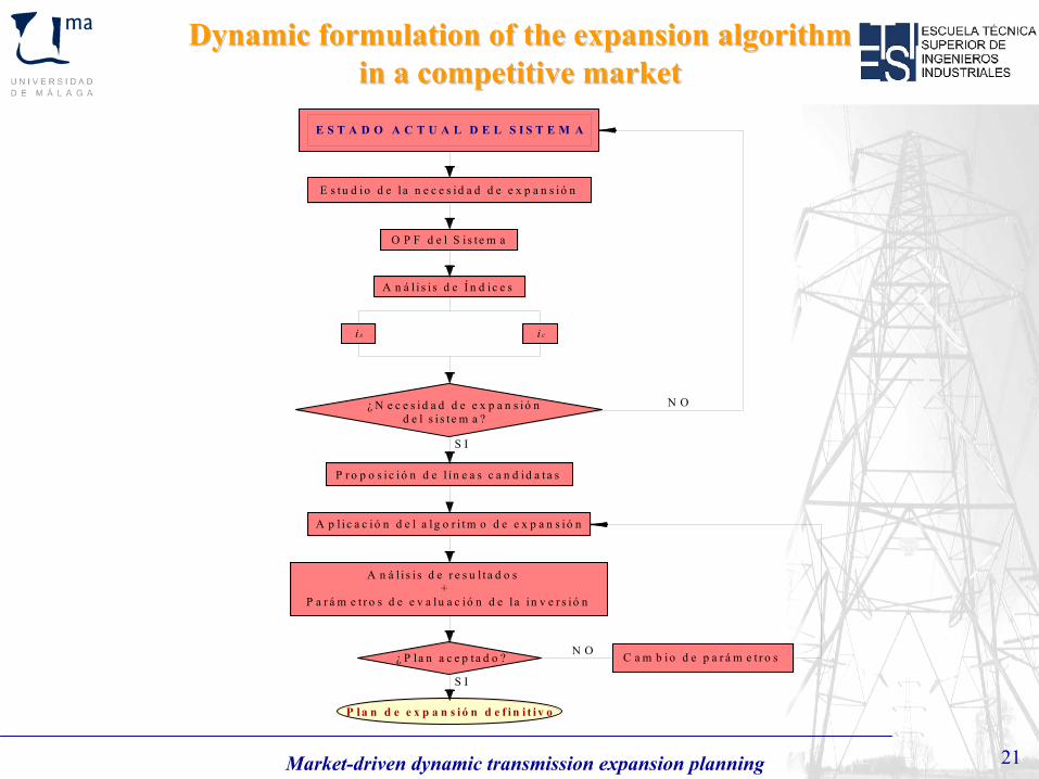
Dynamic formulation of the expansion algorithm Dynamic formulation of the expansion algorithm in a competitive marketin a competitive market
E s tu d i o d e l a n e c e s id a d d e e x p a n s ió n
O P F d e l S i s t e m a
A n á l i s i s d e Í n d i c e s
i s
P r o p o s i c i ó n d e l í n e a s c a n d id a t a s
A p l i c a c ió n d e l a l g o r i t m o d e e x p a n s ió n
¿ N e c e s i d a d d e e x p a n s ió n d e l s i s t e m a ?
E S T A D O A C T U A L D E L S I S T E M A
A n á l i s i s d e r e s u l t a d o s +P a r á m e t r o s d e e v a lu a c ió n d e l a i n v e r s ió n
¿ P la n a c e p t a d o ? C a m b i o d e p a r á m e t r o s
P l a n d e e x p a n s i ó n d e f i n i t i v o
S I
N O
S I
N O
i c
Market-driven dynamic transmission expansion planning 22
MarketMarket--driven transmission expansion planningdriven transmission expansion planning
SummarySummary
Introduction to electrical power systemsIntroduction to electrical power systems
MotivationMotivation
Bibliography searchBibliography search
Dynamic formulation of the expansion algorithm in a competitive marketDynamic formulation of the expansion algorithm in a competitive market
Case studiesCase studies
Conclusions and future workConclusions and future work
2
Modeling of the components of a power system marketModeling of the components of a power system market
Market-driven dynamic transmission expansion planning 23
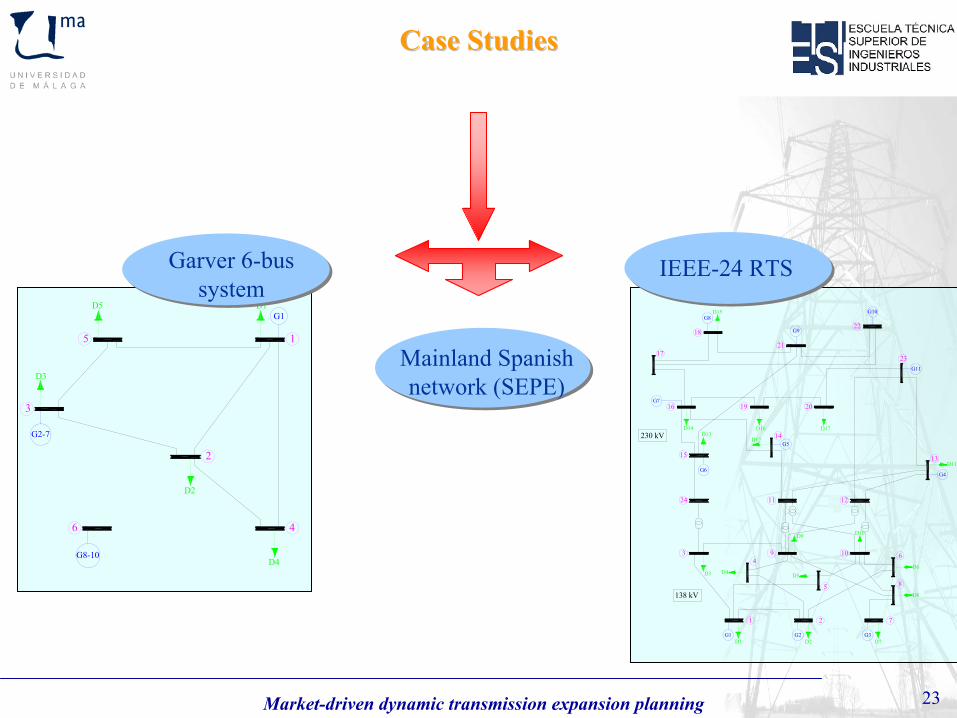
Mainland Spanish network (SEPE)
5
D4
D5G1
3
6
1
2
4
D1
D2
D3
G8-10
G2-7
Garver 6-bussystem
G1
1 2
G2 G3
7
34
5
6
8
9 10
1211
13
14
15
16
17
18
19 20
21
22
23
24
G4G6
G5
G7
G8
G9
G10
G11
D1 D2 D7
D3 D4 D5D6
D8
D9 D10
D11
D12D13
D14
D15
D16 D17
138 kV
230 kV
IEEE-24 RTS
Case StudiesCase Studies
Market-driven dynamic transmission expansion planning 24
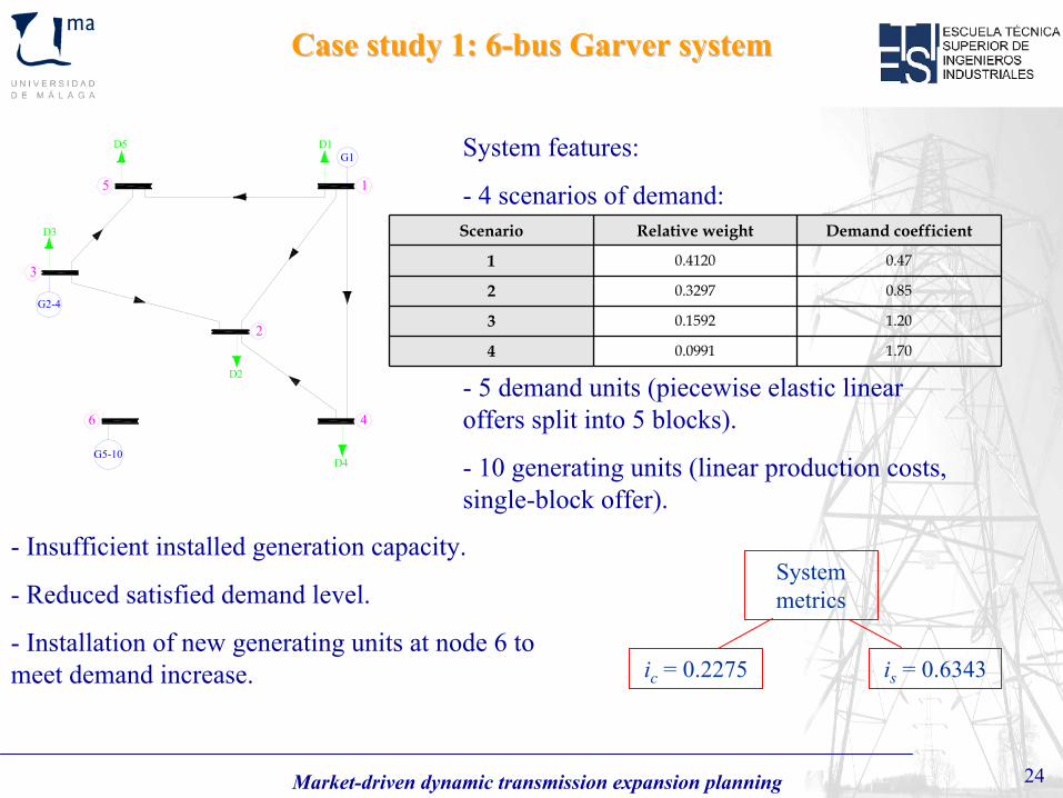
Case study 1: 6Case study 1: 6--bus Garver systembus Garver system
5
D4
D5G1
3
6
1
2
4
D1
D2
D3
G5-10
G2-4
System features:
- 4 scenarios of demand:
-
5 demand units (piecewise elastic linear offers split into 5 blocks).
-
10 generating units (linear production costs, single-block offer).
System metrics
ic
= 0.2275 is
= 0.6343
- Insufficient installed generation capacity.
- Reduced satisfied demand level.
-
Installation of new generating units at node 6 to meet demand increase.
Scenario Relative weight Demand coefficient
1 0.4120 0.47
2 0.3297 0.85
3 0.1592 1.20
4 0.0991 1.70
Market-driven dynamic transmission expansion planning 25
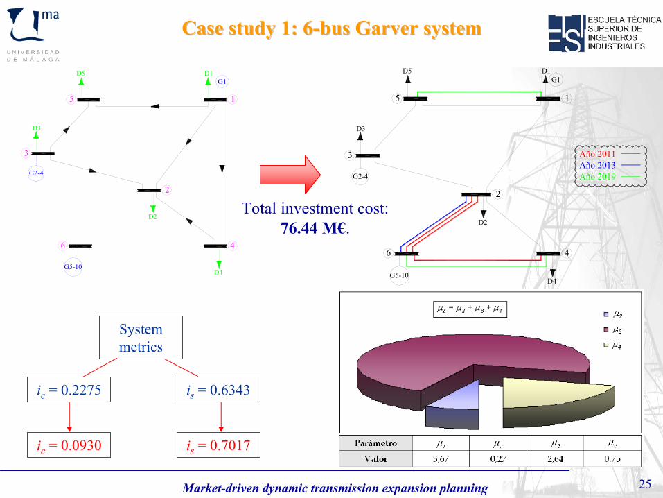
Case study 1: 6Case study 1: 6--bus Garver systembus Garver system
Año 2019Año 2013Año 2011
D5G1
D1
5
D4
3
6
1
2
4
D2
D3
G5-10
G2-4
5
D4
D5G1
3
6
1
2
4
D1
D2
D3
G5-10
G2-4
Total investment cost: 76.44 M€.
System metrics
ic
= 0.2275 is
= 0.6343
ic
= 0.0930 is
= 0.7017
Market-driven dynamic transmission expansion planning 26
( ) ( )( )
( )∑ ∑ ∑∑ ∑ ∑∑ ∑∈ ∈ ∈∀
−∈∀ ∈∀ ∈∀
−∈∀ ∈∀
−+
+
−−
⎥⎥⎦
⎤
⎢⎢⎣
⎡⎟⎟⎠
⎞⎜⎜⎝
⎛
+−
+Y Y L
0
srksrk
)y(C G i0
ibib
D d0
dhdh
y y )k,r,s(yy
yysrk
sr)y(c i b
yy
)y(cG
)y(cG
d hyy
)y(cD
)y(cD)y(c
r1hwK
r1p
r1p
WΩ Ω ΩΩ Ω ΩΩ Ω
σετλλ
Año 2019Año 2013Año 2011
D5G1
D1
5
D4
3
6
1
2
4
D2
D3
G5-10
G2-4
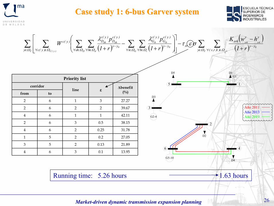
Case study 1: 6Case study 1: 6--bus Garver systembus Garver system
Running time: 5.26 hours 1.63 hours
Priority listcorridor
line ε Δbenefit (%)from to
2 6 1 3 27.27
2 6 2 2 39.67
4 6 1 1 42.11
2 6 3 0.5 38.15
4 6 2 0.25 31.78
1 5 2 0.2 27.05
3 5 2 0.13 21.89
4 6 3 0.1 13.95
Market-driven dynamic transmission expansion planning 27
Case study 2: IEEECase study 2: IEEE--24 RTS24 RTS
G1
1 2
G2 G3
7
34
5
6
8
9 10
1211
13
14
15
16
17
18
19 20
21
22
23
24
G4G6
G5
G7
G8
G9
G10
G11
D1 D2 D7
D3 D4 D5D6
D8
D9 D10
D11
D12D13
D14
D15
D16 D17
138 kV
230 kV
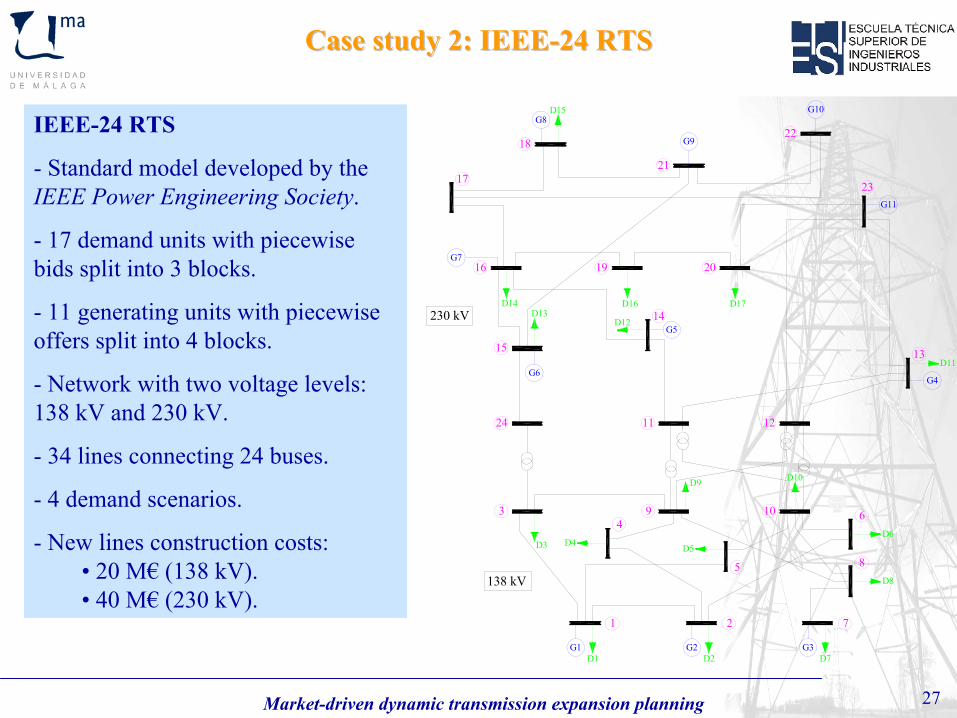
IEEE-24 RTS
-
Standard model developed by the IEEE Power Engineering Society.
-
17 demand units with piecewise bids split into 3 blocks.
-
11 generating units with piecewise offers split into 4 blocks.
-
Network with two voltage levels: 138 kV and 230 kV.
- 34 lines connecting 24 buses.
- 4 demand scenarios.
- New lines construction costs: • 20 M€
(138 kV).
• 40 M€
(230 kV).
Market-driven dynamic transmission expansion planning 28
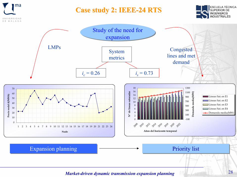
Case study 2: IEEECase study 2: IEEE--24 RTS24 RTS
Study of the need for expansion
System metrics
ic
= 0.26 is
= 0.73
LMPs Congested lines and met
demand
02468
1012141618
2008
2010
2012
2014
2016
2018
2020
2022
Años del horizonte temporalN
º de
líne
as s
atur
adas
-100
100
300
500
700
900
1100
1300
Dem
anda
med
ia(M
W)
Líneas Sat. en E1Líneas Sat. en E2Líneas Sat. en E3Líneas Sat. en E4Demanda media(MW)
0
10
20
30
40
50
60
70
1 2 3 4 5 6 7 8 9 10 11 12 13 14 15 16 17 18 19 20 21 22 23 24
Nudo
Prec
io n
odal
(€/M
Wh)
Expansion planningExpansion planning Priority listPriority list

Market-driven dynamic transmission expansion planning 29
Case study 2: IEEECase study 2: IEEE--24 RTS24 RTS
Priority list
OrderCorridor
Line ε Δbenefit (%)from to
1 1 5 2 1.70 1.02
2 20 23 2 1.60 2.73
3 1 5 3 1.50 3.48
4 2 4 2 1.20 3.82
5 2 4 3 1.00 3.84
6 2 6 2 0.85 3.69
7 20 23 3 0.80 3.21
8 2 6 3 0.60 2.77
9 18 21 2 0.36 1.09
10 16 17 2
0.32 -4.2911 16 19 2
12 17 22 2
13 3 9 2 0.25 -5.26
14 17 22 3 0.23 -7.30
15 7 8 2 0.22 -8.32
Market-driven dynamic transmission expansion planning 30
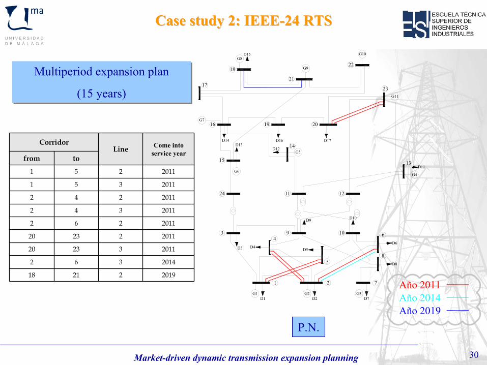
Case study 2: IEEECase study 2: IEEE--24 RTS24 RTS
G6
G5
G7
G8
G9
G10
G11
D9 D10
D11
D12D13
D14
D15
D16 D17
Año 2011Año 2014Año 2019
G1
1 2
G2 G3
7
34
5
6
8
9 10
D1 D2 D7
D3 D4 D5D6
D8
1211
13
14
15
16
17
18
19 20
21
22
23
24
G4
Multiperiod expansion plan
(15 years)
Multiperiod expansion plan
(15 years)
P.N.
CorridorLine Come into
service yearfrom to
1 5 2 2011
1 5 3 2011
2 4 2 2011
2 4 3 2011
2 6 2 2011
20 23 2 2011
20 23 3 2011
2 6 3 2014
18 21 2 2019
Market-driven dynamic transmission expansion planning 31
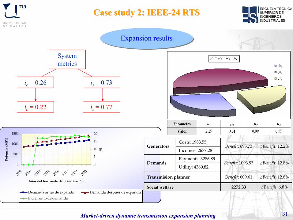
Case study 2: IEEECase study 2: IEEE--24 RTS24 RTS
Expansion results
System metrics
ic
= 0.26 is
= 0.73
ic
= 0.22 is
= 0.77
0
500
1000
1500
2008
2010
2012
2014
2016
2018
2020
2022
Años del horizonte de planificación
Pote
ncia
(MW
)
0
5
10
15
20
%
Demanda antes de expandir Demanda después de expandirIncremento de demanda
GeneratorsCosts: 1983.55
Benefit: 693.73 ΔBenefit: 12.2%Incomes: 2677.28
DemandsPayments: 3286.89
Benefit: 1093.93 ΔBenefit: 12.8%Utility: 4380.82
Transmision planner Benefit: 609.61 ΔBenefit: 12.8%
Social welfare 2272.33 ΔBenefit: 6.8%
Market-driven dynamic transmission expansion planning 32
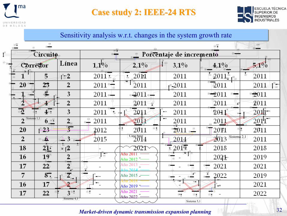
Case study 2: IEEECase study 2: IEEE--24 RTS24 RTS
Sensitivity analysis w.r.t. changes in the system growth rateSensitivity analysis w.r.t. changes in the system growth rate
G1
1 2
G2 G3
7
34
5
6
8
9 10
D1 D2 D7
D3 D4 D5D6
D8
1211
13
14
15
16
17
18
19 20
21
22
23
24
G4G6
G5
G7
G8
G9
G10
G11
D9 D10
D11
D12D13
D14
D15
D16 D17
Sistema 1,1
109
8
6
5
43
7
G3G2
21
G1
Sistema 2,1
D17D16
D15
D14D13
D12
D11
D10D9
G11
G10
G9
G8
G7
G5
G6G4
24
23
22
21
2019
18
17
16
15
14
13
11 12
D8
D6D5D4D3
D7D2D1
D17D16
D15
D14D13
D12
D10D9
G11
G10
G9
G8
G7
G5
G6G4
24
23
22
21
2019
18
17
16
15
14
13
11 12
D8
D6D5D4D3
D7D2D1
109
8
6
5
43
7
G3G2
21
G1
Caso base
15
14
13
11 12
D8
D6D5D4D3
D7D2D1
109
8
6
5
43
7
G3G2
21
G1
Sistema 4,1
D17D16
D15
D14D13
D12
D11
D10D9
G11
G10
G9
G8
G7
G5
G6G4
24
23
22
21
2019
18
17
16
G1
1 2
G2 G3
7
34
5
6
8
9 10
D1 D2 D7
D3 D4 D5D6
D8
1211
13
14
15
16
17
18
19 20
21
22
23
24
G4G6
G5
G7
G8
G9
G10
G11
D9 D10
D11
D12D13
D14
D15
D16 D17
Sistema 5,1
Año 2021
Año 2018Año 2015
Año 2013
Año 2019
Año 2014
Año 2011
Año 2022
Año 2012
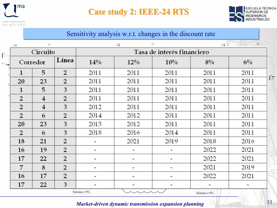
Market-driven dynamic transmission expansion planning 33
Sensitivity analysis w.r.t. changes in the discount rateSensitivity analysis w.r.t. changes in the discount rate
Case study 2: IEEECase study 2: IEEE--24 RTS24 RTS
G8
G9
G10
G11
D9 D10
D11
D12D13
D14
D15
D16 D17
Sistema i=14%
G1
1 2
G2 G3
7
34
5
6
8
9 10
D1 D2 D7
D3 D4 D5D6
D8
1211
13
14
15
16
17
18
19 20
21
22
23
24
G4G6
G5
G7
Sistema i=12%
D17D16
D15
D14D13
D12
D11
D10D9
G11
G10
G9
G8
G7
G5
G6G4
24
23
22
21
2019
18
17
16
15
14
13
11 12
D8
D6D5D4D3
D7D2D1
109
8
6
5
43
7
G3G2
21
G1
D17D16
D15
D14D13
D12
D10D9
G11
G10
G9
G8
G7
G5
G6G4
24
23
22
21
2019
18
17
16
15
14
13
11 12
D8
D6D5D4D3
D7D2D1
109
8
6
5
43
7
G3G2
21
G1
Caso base
D4 D5D6
D8
1211
13
14
15
16
17
18
19 20
21
22
23
24
G4G6
G5
G7
G8
G9
G10
G11
D9 D10
D11
D12D13
D14
D15
D16 D17
Sistema i=6%
G1
1 2
G2 G3
7
34
5
6
8
9 10
D1 D2 D7
D3
24
23
22
21
2019
18
17
16
15
14
13
11 12
D8
D6D5D4D3
D7D2D1
109
8
6
5
43
7
G3G2
21
G1
Sistema i=8%
D17D16
D15
D14D13
D12
D11
D10D9
G11
G10
G9
G8
G7
G5
G6G4
Año 2012
Año 2022
Año 2011
Año 2014
Año 2019
Año 2013
Año 2016Año 2018
Año 2021
Market-driven dynamic transmission expansion planning 34
Case study 3: SEPECase study 3: SEPE
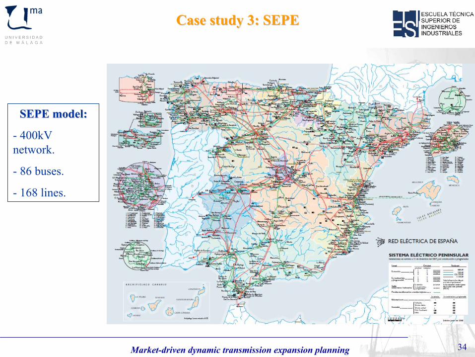
SEPE model:SEPE model:
-
400kV network.
- 86 buses.
- 168 lines.
Market-driven dynamic transmission expansion planning 35
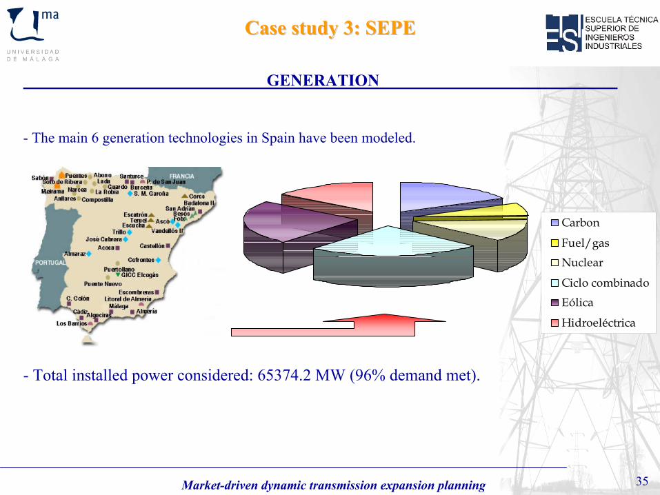
GENERATION
- The main 6 generation technologies in Spain have been modeled.
- Total installed power considered: 65374.2 MW
(96% demand met).
Carbon
Fuel/gas
Nuclear
Ciclo combinado
Eólica
Hidroeléctrica
Case study 3: SEPECase study 3: SEPE
Market-driven dynamic transmission expansion planning 36
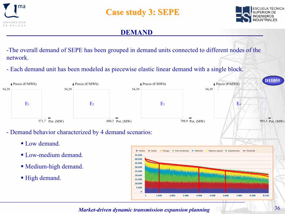
DEMAND
-The overall demand of SEPE has been grouped in demand units connected to different nodes of the network.
- Each demand unit has been modeled as piecewise elastic linear demand with a single block.
- Demand behavior characterized by 4 demand scenarios:
Low demand.
Low-medium demand.
Medium-high demand.
High demand.
Case study 3: SEPECase study 3: SEPE
E1
54,39Precio (€/MWh)
Pot. (MW)571,7 680,3 Pot. (MW)
Precio (€/MWh)54,39
E2
788,9 Pot. (MW)
Precio (€/MWh)54,39
E3
903,3 Pot. (MW)
Precio (€/MWh)54,39
E4
D11055
Market-driven dynamic transmission expansion planning 37
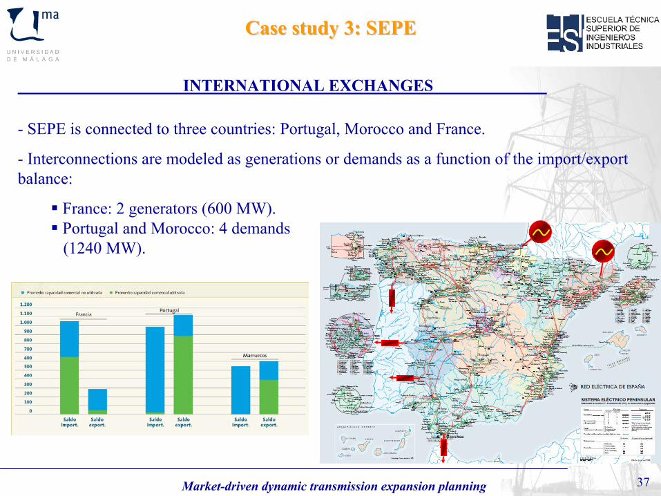
INTERNATIONAL EXCHANGES
- SEPE is connected to three countries: Portugal, Morocco and France.
-
Interconnections are modeled as generations or demands as a function of the import/export balance:
France: 2 generators (600 MW).Portugal and Morocco: 4 demands (1240 MW).
Case study 3: SEPECase study 3: SEPE
Market-driven dynamic transmission expansion planning 38
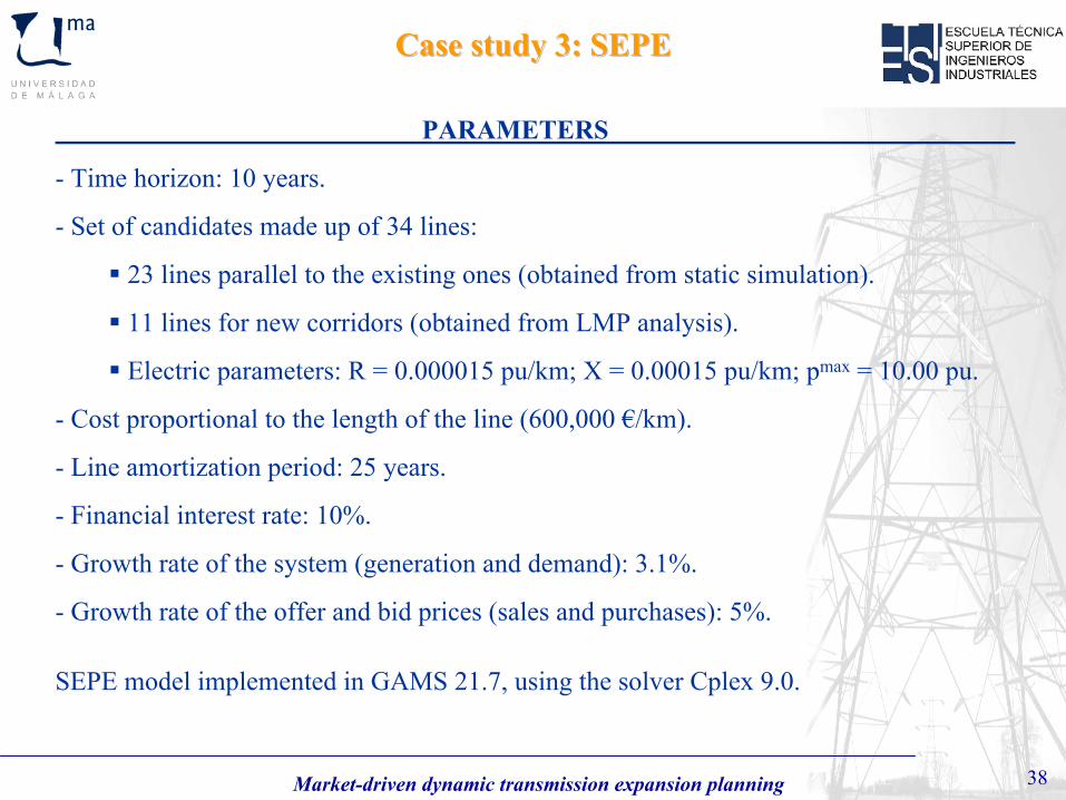
PARAMETERS
- Time horizon: 10 years.
- Set of candidates made up of 34 lines:
23 lines parallel to the existing ones (obtained from static simulation).
11 lines for new corridors (obtained from LMP analysis).
Electric parameters: R = 0.000015 pu/km; X = 0.00015 pu/km; pmax = 10.00 pu.
- Cost proportional to the length of the line (600,000 €/km).
- Line amortization period: 25 years.
- Financial interest rate: 10%.
- Growth rate of the system (generation and demand): 3.1%.
- Growth rate of the offer and bid prices (sales and purchases): 5%.
SEPE model implemented in GAMS 21.7, using the solver Cplex 9.0.
Case study 3: SEPECase study 3: SEPE
Market-driven dynamic transmission expansion planning 39
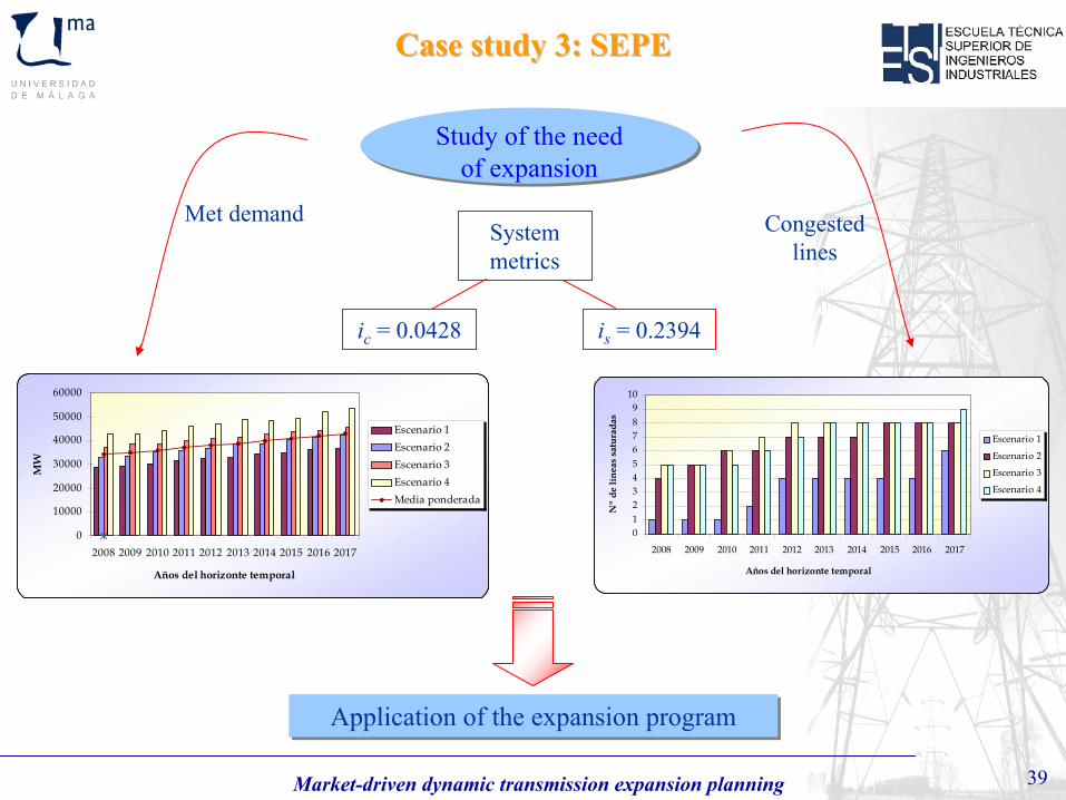
Study of the need of expansion
System metrics
ic
= 0.0428 is
= 0.2394
0
10000
20000
30000
40000
50000
60000
2008 2009 2010 2011 2012 2013 2014 2015 2016 2017
Años del horizonte temporal
MW
Escenario 1Escenario 2Escenario 3Escenario 4Media ponderada
Met demand
0123456789
10
2008 2009 2010 2011 2012 2013 2014 2015 2016 2017
Años del horizonte temporal
Nº
de lí
neas
sat
urad
as
Escenario 1
Escenario 2
Escenario 3
Escenario 4
Congested lines
Case study 3: SEPECase study 3: SEPE
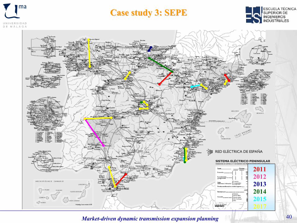
Application of the expansion programApplication of the expansion program
Market-driven dynamic transmission expansion planning 40
201120122013
20152014
2017
Case study 3: SEPECase study 3: SEPE
Market-driven dynamic transmission expansion planning 41
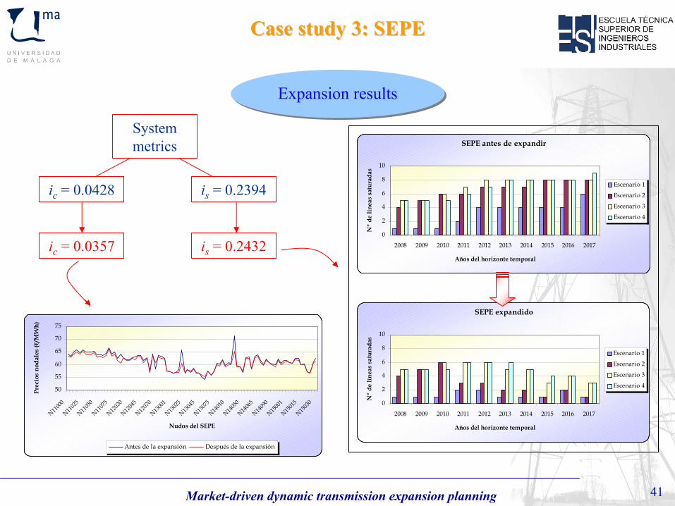
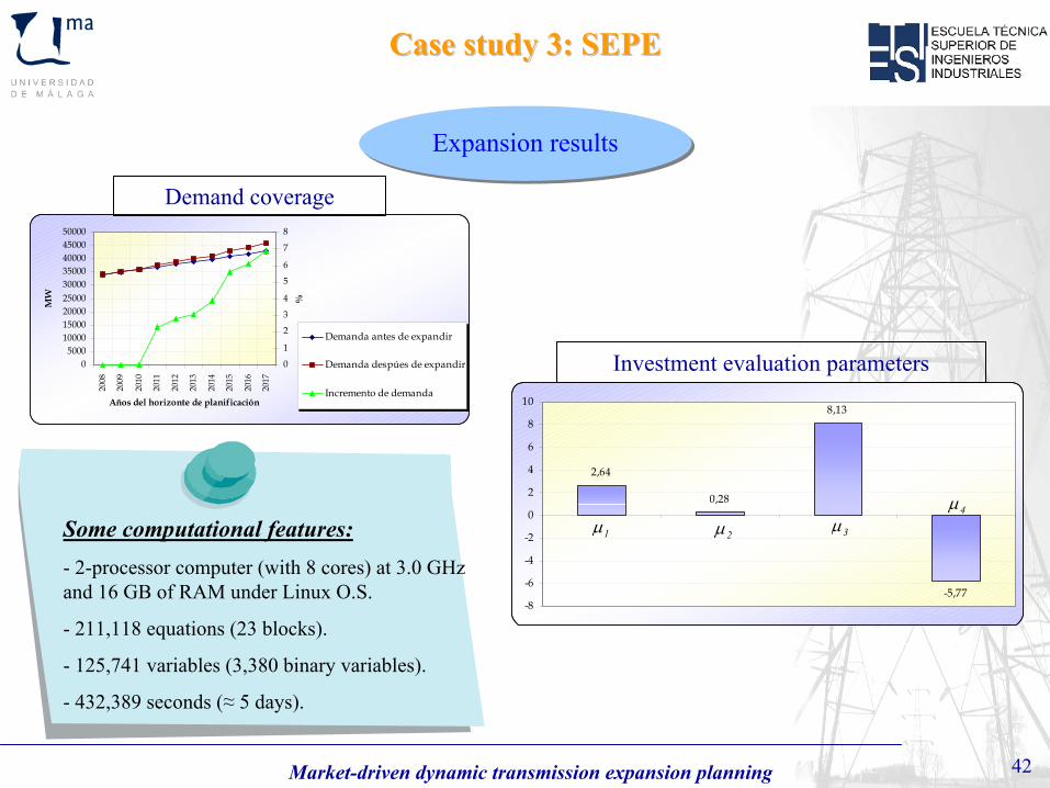
Expansion results
SEPE antes de expandir
0
2
4
6
8
10
2008 2009 2010 2011 2012 2013 2014 2015 2016 2017
Años del horizonte temporal
Nº
de lí
neas
sat
urad
as
Escenario 1
Escenario 2
Escenario 3
Escenario 4
SEPE expandido
0
2
4
6
8
10
2008 2009 2010 2011 2012 2013 2014 2015 2016 2017
Años del horizonte temporal
Nº
de lí
neas
sat
urad
as
Escenario 1
Escenario 2
Escenario 3
Escenario 4
System metrics
ic
= 0.0428 is
= 0.2394
ic
= 0.0357 is
= 0.2432
Case study 3: SEPECase study 3: SEPE
50
55
60
65
70
75
N1100
0N11
025
N1105
0N11
075
N1202
0N12
045
N1207
0N13
001
N1302
5N13
045
N1307
5N14
010
N1405
0 N14
065
N1409
0N15
001
N1501
5N15
030
Nudos del SEPE
Prec
ios
noda
les
(€/M
Wh)
Antes de la expansión Después de la expansión
Market-driven dynamic transmission expansion planning 42
Expansion results
05000
100001500020000250003000035000400004500050000
2008
2009
2010
2011
2012
2013
2014
2015
2016
2017
Años del horizonte de planificación
MW
0
1
2
3
4
5
6
7
8
%
Demanda antes de expandir
Demanda despúes de expandir
Incremento de demanda
Demand coverage
2,64
0,28
8,13
-5,77-8
-6
-4
-2
0
2
4
6
8
10
Investment evaluation parameters
Some computational features:-
2-processor computer (with 8 cores) at 3.0 GHz and 16 GB of RAM under Linux O.S.
- 211,118 equations (23 blocks).
- 125,741
variables (3,380 binary variables).
- 432,389 seconds (≈
5 days).
1μ 2μ 3μ4μ
Case study 3: SEPECase study 3: SEPE
Market-driven dynamic transmission expansion planning 43
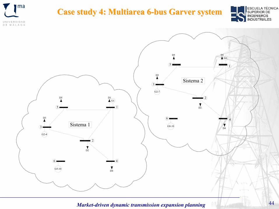
Case study 4: Multiarea 6Case study 4: Multiarea 6--bus Garver systembus Garver system
- New supranational electrical networks interrelated with each other.
- Examples:
EU electricity market (UCTE).
Australian market.
Mercosur (Argentina, Brazil, Paraguay and Uruguay).
Central America electricity market.
U.S. Regional Transmission Organizations.
- Fundamental driver Economics:
• Exploitation of economical mutually beneficial transactions between
systems.
• Increased safety and cost reduction by interconnecting systems.
NEED TO CONSIDER THE INFLUENCE OF INTERCONNECTIONS BETWEEN SYSTEMS
Multiarea expansionMultiarea expansion
Market-driven dynamic transmission expansion planning 44
D4
3
6
1
2
4
D2
D3
G5-10
G2-4
G2-7
G8-10
D3
D2
4
2
1
6
3
G1D5
D4
5
Sistema 2
Sistema 1
D1
D5G1
D1
5
Case study 4: Multiarea 6Case study 4: Multiarea 6--bus Garver systembus Garver system
Market-driven dynamic transmission expansion planning 45
Case study 4: Multiarea 6Case study 4: Multiarea 6--bus Garver systembus Garver system
5
D4
D5G1
3
6
1
2
4
D2
D3
G8-10
G2-7
G2-4
G5-10
D3
D2
4
2
1
6
3
D4
5
D1G1
D5
D1
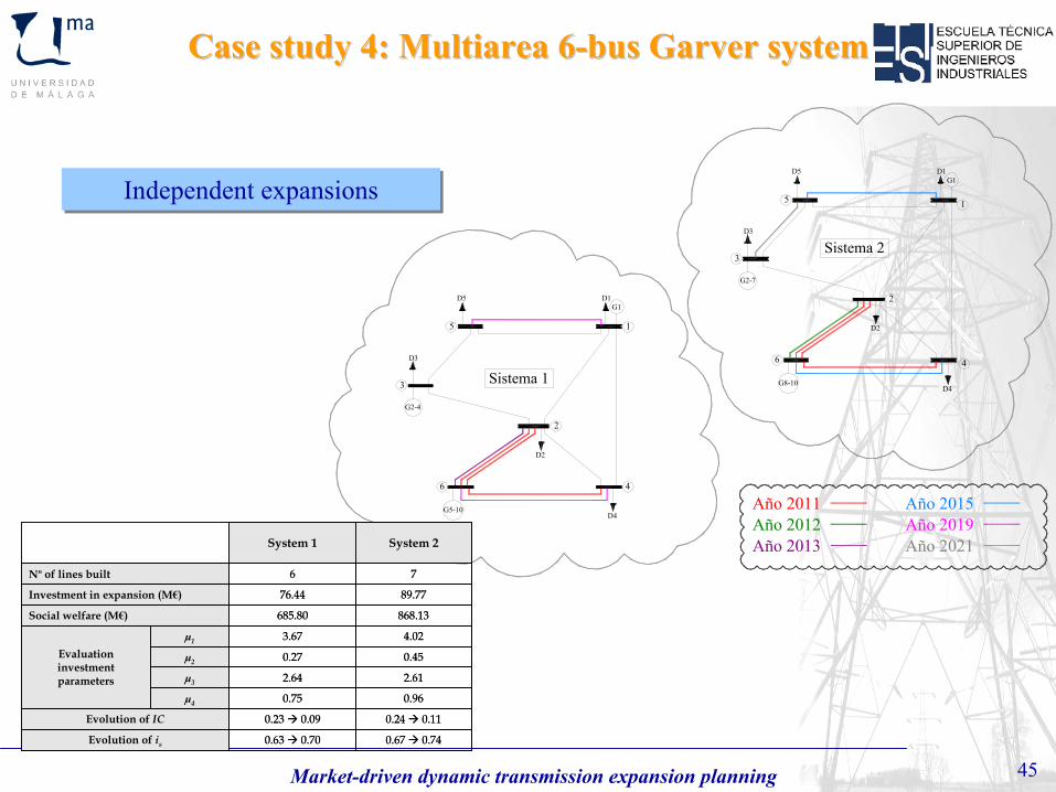
Año 2021Año 2012Año 2013
Año 2015Año 2011Año 2019
Sistema 1
Sistema 2
Independent expansionsIndependent expansions
0.67 0.740.63 0.70Evolution of is
0.24 0.110.23 0.09Evolution of IC
0.960.75μ4
2.612.64μ3
0.450.27μ2
4.023.67μ1Evaluationinvestmentparameters
868.13685.80Social welfare (M€)
89.7776.44Investment in expansion (M€)
76Nº of lines built
System 2System 1
0.67 0.740.63 0.70Evolution of is
0.24 0.110.23 0.09Evolution of IC
0.960.75μ4
2.612.64μ3
0.450.27μ2
4.023.67μ1Evaluationinvestmentparameters
868.13685.80Social welfare (M€)
89.7776.44Investment in expansion (M€)
76Nº of lines built
System 2System 1
Market-driven dynamic transmission expansion planning 46
Case study 4: Multiarea 6Case study 4: Multiarea 6--bus Garver systembus Garver system
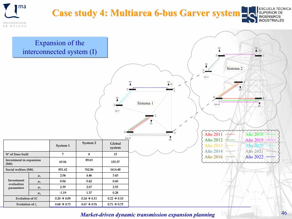
Año 2022Año 2021Año 2020Año 2019
Año 2011
Año 2013
Año 2018
G2-7
G8-10
D3
D2
4
2
1
6
3
G1D5
D4
5
G2-7
G8-10
D3
D2
D1
4
2
1
6
3
G1D5
D4
5
Sistema 1
Sistema 2
Año 2012
Año 2016
D1
Año 2014
Expansion of the interconnected system (I)
Expansion of the interconnected system (I)
0.71 0.750.67 0.760.68 0.73Evolution of is
0.22 0.100.24 0.110.20 0.09Evolution of IC
0.281.37-1.19μ4
2.552.672.39μ3
0.600.420.84μ2
3.434.462.04μ1Investmentevaluationparameters
1614.48762.86851.62Social welfare (M€)
155.5789.6365.94Investment in expansion(M€)
1587Nº of lines built
Global system
System 2System 1
Market-driven dynamic transmission expansion planning 47
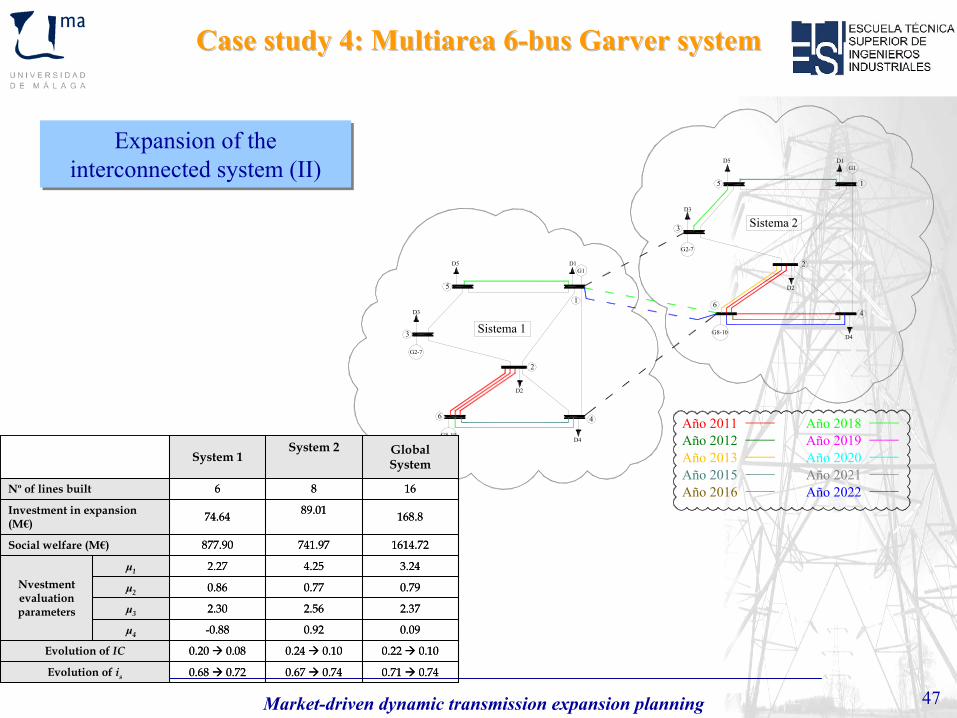
Año 2015
D1
Año 2016
Año 2012
Sistema 2
Sistema 1
5
D4
D5G1
3
6
1
2
4
D1
D2
D3
G8-10
G2-7
5
D4
D5G1
3
6
1
2
4
D2
D3
G8-10
G2-7
Año 2018
Año 2013
Año 2011Año 2019Año 2020Año 2021Año 2022
Expansion of the interconnected system (II)
Expansion of the interconnected system (II)
Case study 4: Multiarea 6Case study 4: Multiarea 6--bus Garver systembus Garver system
0.71 0.740.67 0.740.68 0.72Evolution of is
0.22 0.100.24 0.100.20 0.08Evolution of IC
0.090.92-0.88μ4
2.372.562.30μ3
0.790.770.86μ2
3.244.252.27μ1Nvestmentevaluationparameters
1614.72741.97877.90Social welfare (M€)
168.889.0174.64Investment in expansion(M€)
1686Nº of lines built
Global System
System 2System 1
Market-driven dynamic transmission expansion planning 48
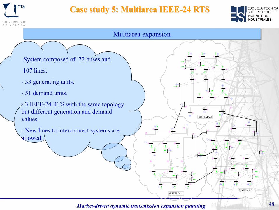
Multiarea expansionMultiarea expansion
-System composed of 72 buses and
107 lines.
- 33 generating units.
- 51 demand units.
-
3 IEEE-24 RTS with the same topology but different generation and demand values.
-
New lines to interconnect systems are allowed.
G1
12
G2G3
7
34
5
6
8
910
12 11
13
14
15
16
17
18
1920
21
22
23
24
G4G6
G5
G7
G8
G9
G10
G11
D1D2D7
D3D4D5D6
D8
D9D10
D11
D12D13
D14
D15
D16D17
SISTEMA 3
D17D16
D15
D14D13
D12
D11
D10D9
D8
D6D5D4D3
D7D2D1
G11
G10
G9
G8
G7
G5
G6G4
24
23
22
21
2019
18
17
16
15
14
13
11 12
109
8
6
5
43
7
G3G2
21
G1
G1
1 2
G2 G3
7
3
4
5
6
8
9 10
1211
13
14
15
16
17
18
19 20
21
22
23
24
G4G6
G5
G7
G8
G9
G10
G11
D1 D2 D7
D3 D4 D5D6
D8
D9 D10
D11
D12D13
D14
D15
D16 D17
SISTEMA 1SISTEMA 2
Case study 5: Multiarea IEEECase study 5: Multiarea IEEE--24 RTS24 RTS
Market-driven dynamic transmission expansion planning 49
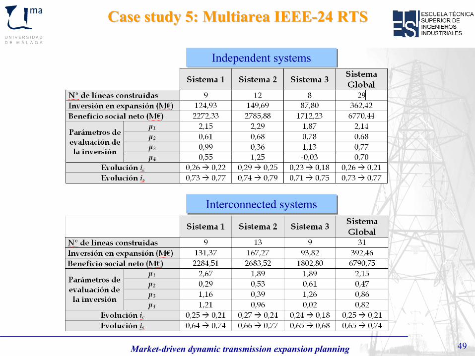
Interconnected systemsInterconnected systems
Independent systemsIndependent systems
Case study 5: Multiarea IEEECase study 5: Multiarea IEEE--24 RTS24 RTS
Market-driven dynamic transmission expansion planning 50
MarketMarket--driven transmission expansion planningdriven transmission expansion planning
SummarySummary
Introduction to electrical power systemsIntroduction to electrical power systems
MotivationMotivation
Bibliography searchBibliography search
Dynamic formulation of the expansion algorithm in a competitive marketDynamic formulation of the expansion algorithm in a competitive market
Case studiesCase studies
Conclusions and future workConclusions and future work
2
Modeling of the components of a power system marketModeling of the components of a power system market
Market-driven dynamic transmission expansion planning 51
A planning algorithm has been designed to develop multiperiod expansion plans including both classic technical operation constraints and new realistic economic and financial constraints.
Implementation of different demand scenarios to characterize the behavior of each year of the planning horizon.
The influence of interconnections between electrical networks has been analyzed related to the individual system expansions (as compared an overall multi-area expansion)
The developed tool has beeen proven useful and robust as tested
with realistic cases.
ConclusionsConclusions
Market-driven dynamic transmission expansion planning 52
Introduction of safety and reliability criteria.
Demand forecasting.
Connection of GAMS with friendly visual interfaces (PowerWorld).
Development of a decentralized multi-area expansion algorithm based on Lagrangian relaxation techniques.
Future workFuture work
Market-driven dynamic transmission expansion planning 53
Market-driven dynamic transmission expansion planning
MarketMarket--driven dynamic transmission driven dynamic transmission expansion planningexpansion planning
Ing. Álvaro Martínez Valle (UMA)Dr. José Antonio Aguado Sánchez (UMA)
Dr. Sebastián de la Torre Fazio (UMA)Dr. Javier Contreras Sanz (UCLM)
Ing. Álvaro Martínez Valle (UMA)Dr. José Antonio Aguado Sánchez (UMA)
Dr. Sebastián de la Torre Fazio (UMA)Dr. Javier Contreras Sanz (UCLM)
ESCUELA TÉCNICA SUPERIOR DE INGENIEROS INDUSTRIALESUNIVERSIDAD DE CASTILLA – LA MANCHA
13071 Ciudad Real, Spain
INFORMS 2009 Annual Meeting, San Diego, 11-14 October, 2009
ESCUELA TÉCNICA SUPERIOR DE INGENIEROS INDUSTRIALESUNIVERSIDAD DE MÁLAGA
29071 Málaga, Spain