TI 2012-139/II Tinbergen Institute Discussion Paper

Market Power in Bilateral Oligopoly Markets with Nonexpandable Infrastructures

Yukihiko Funaki1

Harold Houba2

Evgenia Motchenkova2

1 School of Political Science and Economics, Waseda University, Japan; 2 Faculty of Economics and Business Administration, VU University Amsterdam, and Tinbergen Institute.

Tinbergen Institute is the graduate school and research institute in economics of Erasmus University Rotterdam, the University of Amsterdam and VU University Amsterdam. More TI discussion papers can be downloaded at http://www.tinbergen.nl Tinbergen Institute has two locations: Tinbergen Institute Amsterdam Gustav Mahlerplein 117 1082 MS Amsterdam The Netherlands Tel.: +31(0)20 525 1600 Tinbergen Institute Rotterdam Burg. Oudlaan 50 3062 PA Rotterdam The Netherlands Tel.: +31(0)10 408 8900 Fax: +31(0)10 408 9031

Duisenberg school of finance is a collaboration of the Dutch financial sector and universities, with the ambition to support innovative research and offer top quality academic education in core areas of finance.

DSF research papers can be downloaded at: http://www.dsf.nl/ Duisenberg school of finance Gustav Mahlerplein 117 1082 MS Amsterdam The Netherlands Tel.: +31(0)20 525 8579

Market Power in Bilateral Oligopoly Markets withNonexpandable Infrastructures

Yukihiko Funaki∗

Waseda UniversityHarold Houba†

VU University Amsterdamand Tinbergen Institute

Evgenia Motchenkova‡

VU University Amsterdamand Tinbergen Institute

September, 2012

Abstract

We consider price-fee competition in bilateral oligopolies with perfectly-divisible goods,non-expandable infrastructures, concentrated agents on both sides, and constant mar-ginal costs. We define and characterize stable market outcomes. Buyers exclusivelytrade with the supplier with whom they achieve maximal bilateral joint welfare. Pricesequal marginal costs. Threats to switch suppliers set maximal fees. These also arisefrom a negotiation model that extends price competition. Competition in both pricesand fees necessarily emerges. It improves welfare compared to price competition, butconsumer surpluses do not increase. The minimal infrastructure achieving maximalaggregate welfare differs from the one that protects buyers most.

JEL Classification:C78, L10, L14, D43, R10.

Keywords:Assignment Games, Infrastructure, Negotiations, Non-linear pricing, Market Power

∗School of Political Science and Economics, Waseda University. Email: funaki@waseda.jp.†Department of Econometrics, VU University Amsterdam, De Boelelaan 1105, 1081 HV Amsterdam, the

Netherlands. Email: harold.houba@vu.nl.‡Department of Economics, Vrije Universiteit, De Boelelaan 1105, 1081 HV Amsterdam, Netherlands.

Email: emotchenkova@feweb.vu.nl.

1 Introduction

Oligopolistic competition often requires some infrastructure with costly transportation. This

can vary from costs of postal services when purchasing books or computers from online shops

to physical infrastructure required to transport perfectly-divisible goods such as water, chem-

icals, electricity and natural gas. Often, in such contexts, payments for goods consist of two

parts: a price per unit and a fee, i.e. a fixed monetary amount. Transportation costs

may differ per supplier and per customer, for example tariffs for postal services typically

distinguish between domestic and foreign destinations. Also, product modifications in the

intermediate goods market to meet specifications set by heterogeneous customers can be

treated as relation-specific transport cost. The importance of heterogeneous transportation

costs in trade is not at par with standard microeconomics, with the notable exceptions

of Hotelling (1929), Salop (1979), or Economides (1986) for markets with infinitely-many

small customers and indivisible goods. Also, oligopolistic competition in both prices and

fees receives limited attention. Oi (1971), Schmalensee (1981) and Schmalensee (1982) ana-

lyze two-part pricing for monopoly markets where the supplier lacks information about the

consumers’willingness to pay for a perfectly-divisible good. Two-part pricing in oligopoly

settings with perfect information is studied in e.g. Calem and Spulber (1984), Harrison and

Kline (2001), or Kanemoto (2000). In our study, we analyze competition in both prices

and fees in an oligopolistic market with a finite number of concentrated buyers and suppli-

ers, all heterogeneous, on a given non-expandable infrastructure that is needed to transport

some perfectly-divisible good. Marginal costs of both production and transportation are

constant and relation-specific. One aim of this study is to analyze oligopolistic competition

in prices and fees, the quantities traded and how these are affected by the non-expandable

infrastructure.

Markets with a few concentrated suppliers and a few concentrated buyers, who all can

exercise market power, are referred to as bilateral oligopolies. It is well known that con-

centration on the supply side increases market power and that it has negative consequences

1

for consumer welfare and aggregate social welfare, see e.g. Tirole (1988) or Motta (2004).

Conditions under which these results extend to bilateral oligopolies are derived in e.g. Bloch

and Ghosal (1997), Bloch and Ferrer (2001), or Amir and Bloch (2009). Galbraith (1952) is

probably the first author who has argued that concentrated buyers can also have counter-

vailing power that can restrain the market power of suppliers. Hence, especially in bilateral

oligopolies with high concentration on both sides, the relationship between concentration,

market power and effi ciency is much more complex, and only a few studies have investigated

this relationship both theoretically and empirically. Of those studies, several have tested

the countervailing power hypothesis, and there appears to be evidence that buyer concen-

tration negatively affects the market power of suppliers, see e.g. Scherer and Ross (1990)

for a review of this literature that was initiated by Lustgarten (1975). Also, Schumacher

(1991) supports the countervailing power hypothesis in a study based on US manufacturing

industries. All studies emphasize that threats to switch orders from one supplier to another

strengthen a buyer’s bargaining position.1 A second aim of this study is to investigate the

relationship between market concentration on both sides, market power and effi ciency in

bilateral oligopolies. We also characterize the minimal infrastructure that achieves maximal

aggregate social welfare and the one that protects buyers most from the supply side’s market

power.

As an appropriate equilibrium concept for bilateral oligopolies we propose a stability

concept that balances, on the one hand, generality without too much specific institutional

details to capture a variety of bargaining processes.2 On the other hand, this equilibrium

concept takes into account the essence of market power or bargaining power of suppliers and

buyers, including threats to switch orders from one supplier to another. As the equilibrium

concept, we impose stability against deviating coalitions of traders: prices, fees and traded

1Another threat by which buyers can strengthen their bargaining position is to start upstream productionthemselves. Inderst and Wey (2007) and Dana (2012) investigate the threat of forming buyer groups thatwill act on behalf of their members, which requires some form of either legal or credible commitment. In ourstudy we only look at the threat of switching orders.

2For that reason, we do not impose explicit price setting mechanisms such as in e.g. the market gameproposed in Shapley and Shubik (1977).

2

quantities are in equilibrium if there are no alternative prices, fees and quantities such that

either no buyer wants to join another supplier’s clientele, or no supplier wants to reduce or

expand his clientele. Stability is defined on the non-expandable infrastructure.

We characterize all stable market outcomes and show that these have a lattice structure

and are bilaterally effi cient. Bilateral effi ciency means that positive quantities in each pair-

wise trade maximize the bilateral joint welfare of this pair, which consists of the standard

consumer and producer surplus, taking all other trades as given. Therefore, bilateral effi -

ciency implies relation-specific marginal-cost pricing in order to realize the maximal bilateral

joint welfare. This result implies that all stable market outcomes are also Pareto effi cient:

the equilibrium quantities are the same as if all firms were price-takers. Thus, market power

under oligopolistic competition in prices and fees does not necessarily cause distortions as

opposed to oligopolistic competition in prices, where deadweight losses are unavoidable. This

result is similar to those reported in e.g. Oi (1971), but different from the results in e.g.

Calem and Spulber (1984), or Harrison and Kline (2001).

The relation-specific fee distributes the joint welfare between the buyer and supplier,

where higher fees can be seen as a reflection of higher supply side market power. From

the perspective of buyers, zero fees yield maximal consumer surplus. In any stable market

outcome, suppliers may trade with several buyers. Each buyer, however, exclusively trades

with his most-effi cient supplier, i.e., the one with the lowest cost, on the infrastructure in

order to achieve the maximal bilateral joint welfare, but this makes each buyer vulnerable

to market power exercised by his most-effi cient supplier. Such market power, however, is

limited by each buyer’s threat to trade with his second-effi cient supplier on the infrastructure.

Therefore, a buyer’s maximal fee is bounded from above by the difference of the maximal

bilateral joint welfare levels that can be achieved by trading with his most-effi cient supplier

and second-effi cient supplier. The set of stable fees has a lattice structure. All these results

can be linked to similar results for assignment games in matching markets with indivisible

goods, see Shapley and Shubik (1972), Roth and Sotomayor (1990), Camina (2006), and

3

Sozanski (2006).

The stability concept induces unique relation-specific prices and unique relation-specific

positive quantities traded, but the non-degenerate ranges of relation-specific fees reveal inde-

terminacy. We do not regard indeterminacy as a critique, because it allows for flexibility in

filling in the precise institutional details of the market and the distribution of bargaining or

market power. In the bargaining literature, there are many bargaining protocols that each

induce different market outcomes. In our study, we modify the one-sided proposal-making

model from the literature on matching markets, see e.g. Roth and Sotomayor (1990), to

model extreme market or bargaining power by one side of the market. The modified negoti-

ation model features simultaneous price-fee proposals by agents from one side of the market

to all connected agents on the opposite side of the market and, if accepted, the agents who

accept choose quantities. We are especially interested in the supply side making such propos-

als and compare the outcomes to those arising from oligopolistic (differentiated Bertrand)

price competition. Suppliers propose marginal-cost pricing and the maximal stable fees, all

relation-specific. Buyers accept the offer from their most-effi cient supplier and demand the

joint-welfare maximizing quantities. Compared to oligopolistic price competition, competi-

tion in both prices and fees improves aggregate joint welfare but buyers are not better off.

Finally, when buyers propose, then we have the relation-specific marginal-cost pricing and

no (or zero) fees result. The latter can be seen as the outcome under perfect competition.

Because each buyer only utilizes a single link among his potential trading relations on

the non-expandable infrastructure, we also identify the minimal infrastructure that would

generate maximal aggregate joint welfare among all infrastructures and this only requires

that each buyer is linked to his most-effi cient supplier among all suppliers. To reduce vulner-

ability of buyers to market power exercised by the supply side, we also identify the minimal

infrastructure that would generate the maximal aggregate consumer surplus among all in-

frastructures and this requires that each buyer is linked to his most-effi cient supplier and his

second-most effi cient supplier among all suppliers. In such setting, even though each buyer

4

will never utilize one of his two links, the other link needs to be present in order to have a

credible threat of switching to another supplier.

The current study introduces the framework of bilateral oligopolies and explains the main

ideas of competition in relation-specific prices and fees on a non-expandable infrastructure.

This allows us to offer three major insights: a theory of market competition and market

power in concentrated markets with a non-expandable infrastructure; identification of the

non-expandable infrastructure with maximal buyer protection; and emergence of competition

in prices and fees instead of oligopolistic competition in prices only. We regard a thorough

understanding of non-expandable infrastructures as a first and necessary step towards an

analysis of market power on expandable infrastructures under costly investment. Such analy-

sis will be provided in a companion paper Funaki et al. (2012). Expandable infrastructures

are more appropriate in the setting with less costly investment such as contractual rela-

tionships, software development for heterogeneous clients, or relation-specific investments in

intermediate goods markets to meet heterogeneous buyers’specifications, as discussed in e.g.

Bjornerstedt and Stenneck (2007). Nevertheless, the results for non-expandable infrastruc-

tures are relevant to analyze spot-markets on infrastructures that cannot be expanded in

the short run, such as infrastructure for natural gas and oil, and relation-specific capital

investments.

The paper is organized as follows. Section 2 outlines the model and in section 3 three

motivating examples are provided. Oligopolistic competition in prices and fees on a non-

expandable infrastructure is analyzed in Section 4. Some concluding remarks are left for

Section 5.

2 The model

Consider a market with a finite set S of suppliers, |S| ≥ 1, of some good and a finite set B

of buyers, |B| ≥ 1. We denote an individual supplier as i and an individual buyer as j. The

set of all agents is N = S ∪ B. Each agent in N is either a supplier or a buyer, that is the

5

sets S and B are disjoint, i.e. S ∩B = ∅.

Bilateral trade requires infrastructure that links supplier i and buyer j. Without such

a link, a pair of buyers and suppliers cannot trade. The link between supplier i and buyer

j is denoted ij ≡ (i, j) ∈ S × B, and often we call ij a pair. The set of all potential links

ij is denoted by gN = {ij|ij ∈ S ×B}, which is an undirected graph. An infrastructure g

on N is an arbitrary set of links g ⊆ gN . In particular, the set of all feasible links gN is

called the complete infrastructure and g0 = ∅ represents the absence of any infrastructure.

The collection of all networks is denoted by GN = {g|g ⊆ gN}. In what follows, we think of

infrastructures as some non-expandable infrastructure inherited from the past whose building

costs are sunk. For explanatory reasons, we assume that links are of unlimited capacity. Its

operating and managing costs are assumed to be included in the variable transportation

costs, which are defined below.

In this market, we keep track of trade flows between pairs of linked suppliers and buyers.

For a given infrastructure g ⊆ gN and a pair ij ∈ g, the quantity qij ≥ 0 denotes the

flow of output from supplier i to buyer j. For convenience, we set qij = 0 to represent

the infeasibility of trade for any pair ij /∈ g, and we denote the matrix of all trades on

g ⊆ gN as Q|g = (qij)ij∈S×B ∈ R|S×B|+ . Supplier i’s total production or quantity sold is

qi =∑

j∈B:ij∈g qij. Production and shipping products within any pair takes place against

constant marginal costs that depend upon the identity of the suppliers and buyers. Denote

cij ≥ 0, ij ∈ gN , as the marginal costs of both production and transportation from supplier

i to buyer j. Suppliers may sell their products to multiple buyers. Given trades Q|g on

infrastructure g ⊆ gN , we define the endogenous trade network T (Q|g) ∈ g as all links

ij ∈ g with qij > 0, i.e. all links with positive trade. Supplier i’s active customer network

consists of those buyers with whom this supplier trades positive amounts (and with whom

he is linked to).3 More specific, for supplier i, Ti (Q|g) ⊆ B denotes supplier i’s set of active

buyers j for which qij > 0 on infrastructure g. By definition, this set may be empty if

3The passive or inactive customer network consists of those buyers that are linked to the supplier, andthat do not purchase the product.

6

supplier i has no customers, a singleton in case he has only one customer or it contains

multiple elements in case this supplier has many customers.

Given tradesQ|g on infrastructure g ⊆ gN , buyer j’s total consumption is qj =∑

i∈S:ij∈g qij,

and this buyer has the quasi-linear utility function uj (qj) +mj, where the function uj is in-

creasing in qj and mj is monetary wealth. We consider markets for which the standard

demand as a function of the market price satisfies the Law of Demand, i.e. the demand is

decreasing in its own price e.g. Mas-Colell, Whinston, and Green (1995). This law holds

whenever the utility function is strictly quasi-concave and, by Crouzeix and Lindberg (1986),

this is equivalent to strict concavity of the function uj. For buyer j, Tj (Q|g) ⊆ S denotes

buyer j’s set of active suppliers i for which qij > 0 on infrastructure g.

Competition in this market takes place through relation-specific prices pij ≥ cij and

relation-specific fees fij ≥ 0 for all pairs ij ∈ g. Joint pair-wise welfare within the pair ij ∈ g

can be expressed as the sum of i’s producer surplus (pij − cij) qij+fij and j’s consumer surplus

uj(qij)− pijqij − fij. The maximal joint welfare for the pair ij is given by maxqij≥0 uj(qij)−

cijqij. For technical convenience, we assume a unique joint welfare maximum for each possible

link, that each buyer can rank such welfare maxima over the suppliers in S and we impose

differentiability.

Assumption 1 All cij ≥ 0, ij ∈ gN , are mutually different, and for each buyer j ∈ S, the

function uj is increasing, continuously differentiable and strictly concave in qj, uj (0) = 0,

and u′j (0) > maxi∈S cij.

Recall that the Law of Demand imposes strict concavity, or u′j decreasing, and combined

with continuous differentiability of the utility functions implies that u′j (qij) = cij has at most

one solution. Our assumption on the slope of uj at qj = 0 ensures that, in case of exclusive

trade in the pair ij, a solution exists in which buyer j consumes a positive quantity qij and

that the maximal joint welfare without building costs is positive for each pair ij ∈ gN .

For the initial non-expandable infrastructure g ⊆ gN , the maximal joint welfare associated

with exclusive trade by buyer j with supplier i on the link ij ∈ gN , denoted wg (ij), is defined

7

as

wg (ij) =

{maxqij≥0 [uj(qij)− cijqij] , if ij ∈ g,0, if ij /∈ g.

(1)

For technical convenience, we assume that each buyer and each supplier has an incentive to

trade on at least one link (otherwise we could remove such agent from the model). Addi-

tionally, for all g ⊆ gN , all positive values for wg (ij) are mutually different.

Assumption 2 Each buyer j ∈ B has at least one link i′j ∈ gN such that wg (i′j) > 0, each

supplier i ∈ S has at least one link ij′ ∈ gN such that wg (ij′) > 0, and all positive wg (ij),

ij ∈ gN , are mutually different.

Finally, we denote the matrices of all prices and fees on g ⊆ gN as P |g = (pij)ij∈S×B ∈

R|S×B|+ , respectively, F |g = (fij)ij∈S×B ∈ R|S×B|. The latter means we allow that links might

be subsidized. We set pij = u′j (0) > cij and fij = 0 to represent the infeasibility of trade for

any pair ij /∈ g, which makes qij = 0 the optimal trade in ij /∈ g with supplier i’s producer

surplus equal to zero.

3 Motivating examples

In this section, we discuss competition in both prices and fees in order to stress that it is a

natural extension of the standard oligopolistic competition in prices only.

To set ideas, we first consider the smallest market possible on a non-expandable in-

frastructure, namely the market that consists of a single supplier that is linked to a single

buyer, referred to as supplier 1 and buyer 1 (see the left-hand side of Figure 1). Quantity

q11 will be traded against price p11 and fee f11. Additionally, we suppose that the constant

marginal costs of production and transportation are c11 = 1, and buyer 1 has the quasi-linear

utility function 10√q11− p11q11− f11. The maximal joint welfare in this market, which con-

sists of the sum of the producer and consumer surplus, is twenty-five and it can be reached

by setting the price p11 equal to marginal costs and trading q11 equal to twenty-five units.

8

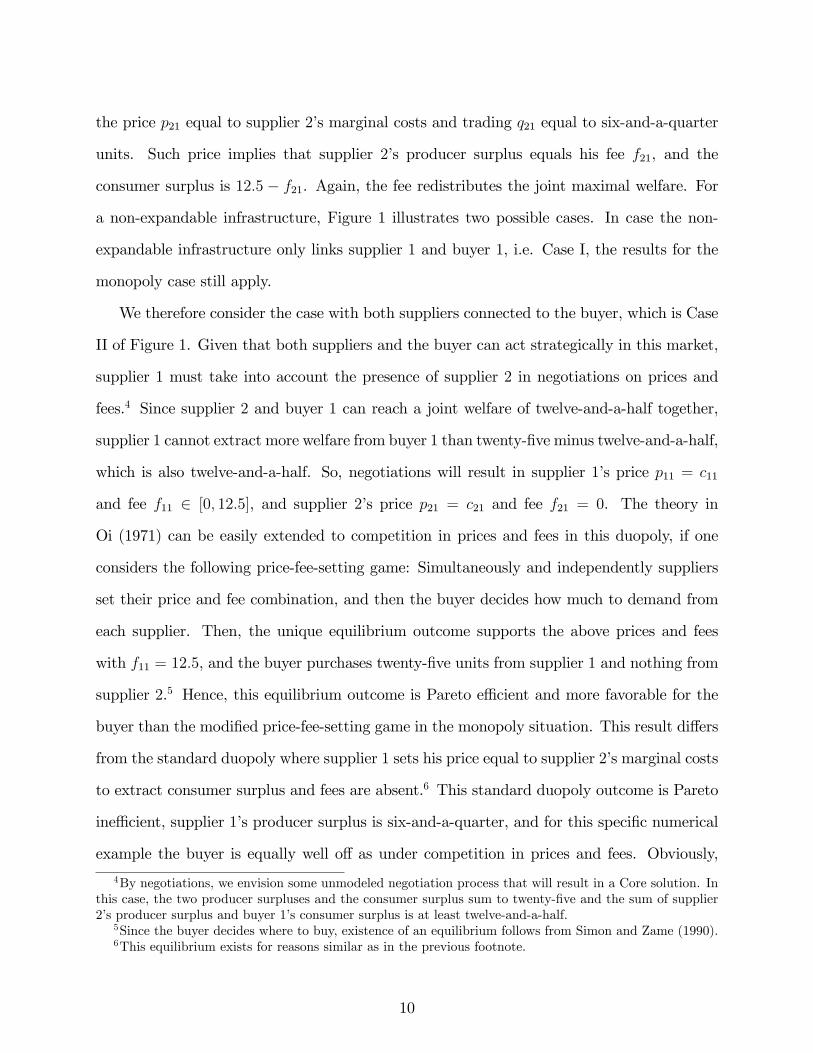
rr rs1

s2

b1-

Case I

rr rs1

s2

b1

������

-

Case II

Figure 1: Supplier 1 is the single supplier in Case I, and one of two suppliers in Case II.

Such price implies that the producer surplus equals the fee f11, and the consumer surplus is

25− f11. The fee therefore determines how the joint maximal welfare is divided within each

pair.

Given that both the supplier and the buyer can act strategically in this market, nego-

tiations will result in marginal-cost pricing p11 = 1 and a fee f11 ∈ [0, 25]. In case of a

monopoly, the theory in Oi (1971) predicts that the supplier will extract the entire consumer

surplus by setting the price p11 = 1 and fee f11 = 25. Hence, the monopoly outcome is Pareto

effi cient, but also very unfavorable for the consumer. This result differs from the standard

monopoly where a price above marginal costs is set to extract consumer surplus and fees are

absent. Standard monopoly pricing is Pareto ineffi cient, but at least the consumer surplus is

positive. The monopoly outcome in Oi (1971) can also be seen as the equilibrium outcome

of a price-fee-setting game in which the supplier sets a price and fee before the buyer decides

how much to buy. By reversing roles in a monopsony, the buyer will set the price p11 = 1

and fee f11 = 0 and it can be supported as the equilibrium outcome of a price-fee-setting

game.

To further illustrate our ideas, we expand the previous situation by introducing a second

supplier who is less effi cient, called supplier 2, who has constant marginal costs of production

and transportation c21 = 2. Supplier 2’s price and fee are p21 and f21. The maximal joint

welfare supplier 2 and buyer 1 can attain when linked, which again consists of the sum

of the producer and consumer surplus, is twelve-and-a-half. It can be reached by setting

9

the price p21 equal to supplier 2’s marginal costs and trading q21 equal to six-and-a-quarter

units. Such price implies that supplier 2’s producer surplus equals his fee f21, and the

consumer surplus is 12.5 − f21. Again, the fee redistributes the joint maximal welfare. For

a non-expandable infrastructure, Figure 1 illustrates two possible cases. In case the non-

expandable infrastructure only links supplier 1 and buyer 1, i.e. Case I, the results for the

monopoly case still apply.

We therefore consider the case with both suppliers connected to the buyer, which is Case

II of Figure 1. Given that both suppliers and the buyer can act strategically in this market,

supplier 1 must take into account the presence of supplier 2 in negotiations on prices and

fees.4 Since supplier 2 and buyer 1 can reach a joint welfare of twelve-and-a-half together,

supplier 1 cannot extract more welfare from buyer 1 than twenty-five minus twelve-and-a-half,

which is also twelve-and-a-half. So, negotiations will result in supplier 1’s price p11 = c11

and fee f11 ∈ [0, 12.5], and supplier 2’s price p21 = c21 and fee f21 = 0. The theory in

Oi (1971) can be easily extended to competition in prices and fees in this duopoly, if one

considers the following price-fee-setting game: Simultaneously and independently suppliers

set their price and fee combination, and then the buyer decides how much to demand from

each supplier. Then, the unique equilibrium outcome supports the above prices and fees

with f11 = 12.5, and the buyer purchases twenty-five units from supplier 1 and nothing from

supplier 2.5 Hence, this equilibrium outcome is Pareto effi cient and more favorable for the

buyer than the modified price-fee-setting game in the monopoly situation. This result differs

from the standard duopoly where supplier 1 sets his price equal to supplier 2’s marginal costs

to extract consumer surplus and fees are absent.6 This standard duopoly outcome is Pareto

ineffi cient, supplier 1’s producer surplus is six-and-a-quarter, and for this specific numerical

example the buyer is equally well off as under competition in prices and fees. Obviously,

4By negotiations, we envision some unmodeled negotiation process that will result in a Core solution. Inthis case, the two producer surpluses and the consumer surplus sum to twenty-five and the sum of supplier2’s producer surplus and buyer 1’s consumer surplus is at least twelve-and-a-half.

5Since the buyer decides where to buy, existence of an equilibrium follows from Simon and Zame (1990).6This equilibrium exists for reasons similar as in the previous footnote.

10

supplier 1 strictly prefers to set a price and fee instead of only a price without a fee. By doing

so, supplier 1 extracts both the consumer surplus and the deadweight loss associated with

standard duopoly pricing. So, the price-fee-setting game on a non-expandable infrastructure

also explains the phenomenon of setting two-part tariffs in practice. By reversing the roles

in a monopsony, the buyer will set p11 = p21 = c11 and f11 = f21 = 0, and supplier 1 will

exclusively trade twenty-five units with buyer 1. Note that adding a third supplier, called

supplier 3, with marginal costs above 2 will not change the above market outcomes. From

here on, we consider three suppliers in our example.

The example makes one point clear: From buyer 1’s perspective, the presence of the link

between supplier 2 is a safeguard against supplier 1’s market power, yet this link will never

be utilized for trade. The link with the third-effi cient supplier 3 is not needed. This is a

fundamental tension between the minimal infrastructure that maximizes social welfare from

trade and the minimal infrastructure that minimizes the supply side’s market power. In

this paper, we develop a theory that characterizes both such minimal infrastructures and we

show that the former is included in the latter.

4 Competition on non-expandable infrastructures

In this section, we analyze oligopolistic competition in prices and fees on a non-expandable

infrastructure. As the equilibrium concept, we modify the concept of a deviating (or block-

ing) coalition to the context of a perfectly divisible good and money on an infrastructure.

We characterize the set of stable market outcomes and show that this set has a lattice struc-

ture. Then, we analyze strategic negotiation models that yield each side’s most preferred

stable market outcome as the unique equilibrium outcome. All these issues are treated in

separate subsections, and the last one contains two important examples. In essence, this

section extends well-known properties of two-sided markets with matching, as surveyed in

e.g. Roth and Sotomayor (1990), to oligopolistic markets with a divisible good and money

on an initial non-expandable infrastructure.

11

4.1 Competition in prices and fees

In this subsection, we introduce the notion of stability of market outcomes to analyze com-

petition in prices and fees. This notion will be applied in characterizing the set of stable

market outcomes in the next subsection.

Economic models of markets are conceived from the fundamental idea that competition

between suppliers and buyers is voluntary and trading is decentralized. Bilateral trade within

a pair of suppliers and buyers is voluntary only if such trade is at least as good as no trade,

because otherwise some agent would be forced to trade against the prevailing conditions.

Bilateral trade is not conducted by a pair of suppliers and buyers in isolation, but takes

place in a market with a possibility to trade with other suppliers and buyers. The presence

of other agents implies outside options for each pair, which presumably affect the conditions

of trade within each pair. For the marriage market and markets with indivisible goods and

money, pair-wise stability would be the appropriate concept, see e.g. Roth and Sotomayor

(1990). In our market, however, the good is perfectly divisible, suppliers may trade with

several buyers, and buyers may trade with several suppliers. Since we also assume that

suppliers and buyers negotiate prices and fees, the Core concept seems more appropriate to

define stability of market outcomes.

Market outcomes consist of prices, fees, and the quantities traded. A market outcome on

a non-expandable infrastructure g ⊆ gN is defined as the triple (P |g, F |g,Q|g). Therefore,

each market outcome generates an endogenous trade network T (Q|g) ∈ g of positive trades.

Recall that supplier i’s active customer network is given by Ti (Q|g) ⊆ B. Similar, buyer

i’s active supplier network is denoted as Tj (Q|g) ⊆ S. The Core concept imposes that any

market outcome on a non-expandable infrastructure is stable if no coalition of suppliers and

buyers wants to break away and trade on their own. To put it differently, all coalitions of

suppliers and buyers weakly prefer the market outcome to trading as a subgroup.

Formally, for coalition C ⊆ N on infrastructure g ⊆ gN , we define the buyer’s quantity

12

purchased from suppliers in coalition C as

qj (C|g) =∑

i∈Tj(Q|g)∩C

qij.

For C = N , we write qj (N |g). Any stable market outcome (P ∗|g, F ∗|g,Q∗|g) yields each

agent a surplus. For supplier i ∈ S, the surplus consists of the revenues and fees collected

from his active customer network Ti (Q∗|g):

∑j∈Ti(Q∗|g)

[(p∗ij − cij)q∗ij + f ∗ij

].

For buyer j ∈ B, the consumer surplus consists of the difference between his utility from

purchasing q∗j (N |g) from his active supplier network Tj (Q|g) and the expenditures and fees

paid to his active suppliers:

uj(q∗j (N |g)

)−

∑i∈Tj(Q∗|g)

[p∗ijq

∗ij + f ∗ij

].

Any market outcome yields each coalition in total a welfare that is equal to the sum of its

members’surpluses. Let C = CS∪CB be the partition of coalition C ⊆ N into suppliers and

buyers. The market outcome (P ∗|g, F ∗|g,Q∗|g) yields coalition C on infrastructure g ⊆ gN

the joint welfare:

∑i∈CS

∑j∈Ti(Q∗|g)

[(p∗ij − cij)q∗ij + f ∗ij

]+∑j∈CB

uj (q∗j (N |g))−

∑i∈Tj(Q∗|g)

[pijq

∗ij + f ∗ij

] . (2)This is coalition C’s joint welfare in case it stays and trades according to market outcome

(P ∗|g, F ∗|g,Q∗|g). Next, suppose coalition C considers to deviate from the above market out-

come through the alternative market outcome (P |g, F |g,Q|g). The surplus for any supplier

in coalition C consists of the revenues and fees collected from his active customer network

restricted to the buyers in coalition C, i.e. for supplier i ∈ CS these are all j ∈ Ti (Q|g)∩CB.

Similarly, the consumer surplus of buyer j ∈ CB consists of the difference between his utility

from purchasing qj (C|g) from his active suppliers in C, i.e. all i ∈ Tj (Q|g) ∩ CS, and the

revenues and fees paid to these active suppliers in C. Since market outcome (P |g, F |g,Q|g)

13

yields each coalition a joint welfare that is equal to the sum of its members’ surpluses,

deviating coalition C’s joint welfare is given by:

∑i∈CS

∑j∈Ti(Q|g)∩CB

[(pij − cij)qij + fij]

+∑j∈CB

uj (qj (C|g))−∑

i∈Tj(Q|g)∩CS

[pijqij + fij]

. (3)The main difference between (2) and (3) is that if a coalition stays it will trade internally in C

and externally of its coalition inN , and if it deviates as a deviating coalition it will only trade

internally. In essence, by deviating coalition C disrupts several external trades. Deviating

is profitable only if such disruptions can be compensated by the surpluses from internal

trades within the coalition. The market outcome is stable if every conceivable deviation is

unprofitable. Given the joint welfare of deviating and non-deviating coalitions, we are ready

to define stability of market outcomes.

Definition 3 Market outcome (P ∗|g, F ∗|g,Q∗|g) on a non-expandable infrastructure g ⊆ gN

is stable if the following condition holds:

For all coalitions C ⊆ N and all (P |g, F |g,Q|g) : (2) ≥ (3) . (4)

Condition (4) expresses the idea that deviating coalitions are unprofitable, and it is a re-

formulation of Core stability for cooperative games in characteristic function form. Although

our setup refrains from explicit market mechanisms and is therefore not a non-cooperative

market game, our stability notion resembles some ideas underlying coalition-proof equilibria,

as proposed in Bernheim et al. (1987) and Bernheim and Whinston (1987). Dana (2012)

characterizes such equilibria in his study of the formation of buyer groups in the presence

of Bertrand price competition. In Section 4.3, we also consider such price competition but

without an ex-ante stage where buyers merge into groups. Several important observations

can be made. For singleton coalitions, each individual agent is weakly better of by trading

than voluntary refraining from such trade. In any stable market outcome, each pair ij ∈ g

can at least achieve its bilateral maximal joint welfare wg (ij) from exclusive bilateral trade

within their pair. For C = N , (4) imposes Pareto effi ciency on the market outcome.

14

4.2 Characterization of stable market outcomes

In this subsection, we provide a full characterization of stable market outcomes on a non-

expandable infrastructure. Furthermore, we establish that the set of stable market outcomes

has a lattice structure.

The characterization of stable market outcomes requires the definition of a buyer’s most-

effi cient and second-(most-)effi cient supplier on the infrastructure, which will be defined in

terms of the maximal joint welfare within pairs of suppliers and buyers. For g ⊆ gN , we

define buyer j’s most-effi cient supplier αj (g) ∈ S on the infrastructure g as the supplier on

g with whom j can attain his largest maximal joint welfare:

wg (αj (g) j) ≥ wg (ij) , for all i ∈ S : ij ∈ g. (5)

Since maximal joint welfare is related to the most-effi cient supplier in terms of marginal

costs, we might alternatively define αj (g) as the supplier for whom cαj(g)j = mini∈S:ij∈g cij,

but (5) captures the key insight needed in Section 5. Buyer j’s most-effi cient supplier αj (g)

is uniquely defined if buyer j is linked through g to one or more suppliers in S. Otherwise,

we impose the convention that αj (g) = 0 denotes supplier "nobody" who has marginal

cost c0j = u′j (0), which makes q0j = 0 optimal, and the pair 0j has maximal joint welfare

wg (0j) = 0. By definition, either cαj(g)j = mini∈S:ij∈g cij or c0j. A buyer’s second-effi cient

supplier is defined similarly. For g ⊆ gN , buyer j’s second-effi cient supplier i ∈ S on the

infrastructure g is the supplier βj (g) on g with whom j can attain his second maximal joint

welfare:

wg(βj (g) j

)≥ wg (ij) , for all i ∈ S\ {αj (g)} : ij ∈ g. (6)

Buyer j’s second-effi cient supplier βj (g) is uniquely defined if buyer j is linked through g to

two or more suppliers in S. Otherwise, and similar as before, we impose the convention that

βj (g) = 0, marginal cost c0j = u′j (0), and the pair 0j has maximal joint welfare wg (0j) = 0.

By definition, either cβj(g)j = mini∈S\{αj(g)}:ij∈g cij or c0j.

We have the following characterization. All proofs are deferred to the appendix.

15

Proposition 4 Market outcome (P ∗|g, F ∗|g,Q∗|g) on a non-expandable infrastructure g ⊆

gN is stable if and only if for all ij ∈ g :

p∗αj(g)j = cαj(g)j, p∗ij ≥ cij, if i 6= αj (g) ,

f ∗αj(g)j ∈[0, wg(αj (g) j)− wg(βj (g) j)

], f ∗ij ≥ 0, if i 6= αj (g) ,

q∗αj(g)j = arg maxqαj(g)j≥0 uj(qαj(g)j)− cαj(g)jqαj(g)j, q∗ij = 0, if i 6= αj (g) .

(7)

For i ∈ S and j ∈ B, supplier i’s active customers network Ti (Q∗|g) = {j ∈ B|i = αj (g)},

and buyer j’s active supplier network Tj (Q∗|g) = {αj (g)}.

From the proof it follows that multiple prices and fees can occur in stable market outcomes

on any link ij ∈ g that will not be utilized for trade. Suppliers on those links know that even

at their lowest acceptable prices and fees, which are p∗ij = cij and f ∗ij = 0, their products

are too expensive from the perspective of buyer j. Therefore, their prices and fees do not

matter.

Proposition 4 implies a very precise prediction of stable market outcomes. Each buyer

exclusively trades with his most-effi cient supplier on the infrastructure against a price that

equals this supplier’s marginal costs and pays a positive fee. This makes buyer j vulnerable

to market power exercised by his most-effi cient supplier. Such market power is limited by the

buyer’s threat to trade with his second-effi cient supplier βj (g) ∈ S ∪ {0} on infrastructure

g. Since supplier βj (g)’s current profit from zero trades with buyer j is zero, buyer j can

seduce supplier βj (g) to trade and by doing so guarantee himself a consumer surplus of

wg(βj (g) j). This limits the market power of the most-effi cient supplier αj (g) in extracting

consumer surplus from the pair αj (g) j ∈ g, because supplier αj (g) must make sure that

buyer j enjoys at least a consumer surplus of wg(βj (g) j) through the link βj (g) j. The most-

effi cient supplier’s fee is therefore bounded from above by the difference between wg(αj (g) j)

and wg(βj (g) j).

Under marginal cost of production and transportation, a supplier’s producer surplus is

equal to the sum of profits per individual link. Supplier i’s profit that can be attributed

to the link ij ∈ g for buyer j ∈ Ti (Q∗|g) is equal to (p∗ij − cij)q

∗ij + f ∗ij = f ∗ij ≥ 0, with

16

strict inequality if Ti (Q∗|g) 6= ∅ and equality otherwise. Supplier i’s aggregate profit is

equal to the sum of these fees, i.e.∑

j∈Ti(Q∗|g) f∗ij, and only supplier’s who are some buyer’s

most-effi cient supplier make positive profits. Then, it is impossible that trade in a link is

subsidized, because f ∗ij < 0 would be an incentive for supplier i to refuse trade on such a

link. Supplier i’s active customer network consists of all buyers for whom this supplier is the

most-effi cient supplier.

We investigate the upper bound on the most-effi cient supplier’s fee for several special

cases. In case j is only linked to a single supplier, then βj (g) = 0 and wg(0j) = 0 im-

ply f ∗αj(g)j ≤ wg(αj (g) j). The absence of a second-effi cient supplier imposes no threat to

supplier αj (g) and hence no limitation to this supplier’s market power. In case j is linked

to two or more suppliers, the difference in marginal costs between the most-effi cient sup-

plier and the second-effi cient supplier matter. If this difference is relatively large, than

wg(βj (g) j) will be relatively small compared to wg(αj (g) j), and the limiting effect of the

threat to switch suppliers will be relatively small. On the other hand, if both the marginal

costs of the most-effi cient supplier and the second-effi cient supplier are relatively close to

each other, then wg(βj (g) j) will be relatively close to wg(αj (g) j) and the presence of the

second-effi cient supplier has a substantial dampening effect on the most-effi cient supplier’s

fee. In case these marginal costs would coincide, which we exclude for convenience, then

wg(βj (g) j) = wg(αj (g) j) and the most-effi cient supplier’s fee must be zero. This implies a

testable hypothesis for industries with almost identical costs structures the equilibrium fees

will be small.

The lower bound on all most-effi cient suppliers’fees also has an interesting interpretation.

In that case the fee f ∗ij = 0 for all ij ∈ g. It can be interpreted as the generalization of the

competitive equilibrium for markets on a non-expandable infrastructure in the sense that all

suppliers follow marginal-cost pricing at zero fees. In this equilibrium, the entire maximal

joint welfare from trade accrues to the buyers, while the suppliers have zero profits. Given

different constant marginal costs, the competitive equilibrium implies relation-specific prices,

17

and zero profits for all suppliers, whether active or not. Obviously, relation-specific prices

are Pareto effi cient and a uniform price per supplier would not.

For some particular market structures, we can be more specific. In case of a monopoly,

i.e. S = {1}, the monopolist’s active customer network is T1 (Q∗|g) = {j ∈ B|1j ∈ g}. By

Assumption 1, each connected buyer has the monopolist as his most-effi cient supplier and

prefers to trade with the monopolist. Since there is no second-effi cient supplier, the range

of fees is maximal. This means that the only countervailing power for buyers depends upon

their negotiation skills. The reverse situation occurs in case of a monopsony, i.e. B = {1},

where only the single link α1 (g) 1 will have positive quantities of trade and the fee will

fully depend upon supplier α1 (g) and buyer i’s negotiation skills. In case of a duopoly, i.e.

S = {1, 2}, it depends upon the infrastructure g ⊆ gN whether each connected buyer is

connected to either supplier 1, or supplier 2 or both suppliers. Those who are connected to

both suppliers will be limited in their maximal fees.

For marriage markets and markets for indivisible goods and money, stable market out-

comes can be ordered because the preferences of each side of the market in evaluating stable

market outcomes are opposed, see e.g. the survey Roth and Sotomayor (1990). In our case

this also holds true: The supply side prefers high fees among the set of stable market out-

comes and the demand side prefers low fees from this set. Since the maximal joint welfare in

the market is constant, an improvement in the profit of any supplier must be at the expense

of the consumer surplus of some of the buyers in this supplier’s active customer network.

Vice versa, an improvement in consumer surplus of some buyer must be at the expense of the

profit of his most-effi cient supplier. Since we can arbitrarily set the fee in each pair (αj (g) j)

to any f ∗αj(g)j ∈[0, wg(αj (g) j)− wg(βj (g) j)

]independent of how we set fees in other pairs

ij ∈ g, the lattice structure for markets with a perfectly divisible good and money on a

non-expandable infrastructure follows immediately from Proposition 4.

Proposition 5 The set of stable market outcomes of Proposition 4 has a lattice struc-

ture. The supply side’s most-preferred stable market outcome has f ∗αj(g)j = wg(αj (g) j) −

18

wg(βj (g) j) for all j ∈ B, and the demand side’s most-preferred stable market outcome has

f ∗αj(g)j = 0 for all i ∈ S.

This result is similar to the results for assignment games in e.g. Roth and Sotomayor (1990).

In fact, an alternative proof of Proposition 5 can be provided that applies cooperative game

theory, and then shows that this game satisfies the conditions that define assignment games.

Since the Core of every assignment game has a lattice structure, this structure immediately

carries over to our model.

Competition in prices and fees allows the following interesting reinterpretation of this

market that also explains the emergence of the lattice structure. Consider a market in which

suppliers and buyers first negotiate a contract that specifies the conditions for trade, which is

unlimited trade against the contract’s specified fixed price. Obviously, contracts that specify

marginal-cost pricing are the most valuable. If we reinterpret the market as a market for the

indivisible good "buyer j has the right to trade with supplier i against price pij", then the

fees f ∗ij represent the standard equilibrium price for markets with indivisible goods such that

each buyer purchases at most one such contract. In such markets, each buyer exclusively

deals with his most-effi cient supplier as if he demands at most one unit of the indivisible

good. The insights provide a different intuition why the lattice structure for stable market

outcomes holds.

4.3 Strategic negotiations

For standard assignment games, the lattice structure of the Core allows to implement each

market side’s most preferred outcome as the unique equilibrium outcome of a strategic ne-

gotiation model, see e.g. Roth and Sotomayor (1990). Since we have also derived a lattice

structure, we will also analyze such strategic models in this subsection. In these models, the

agents of one side of the market all propose prices and fees once, the other side accepts or

rejects, and then the buyers decide from whom to purchase how much against the agreed

upon prices and fees. We characterize the unique equilibrium and relate it to the proposing

19

side’s most preferred stable market outcomes. In case the supply side proposes, we relate

this equilibrium to the Bertrand equilibrium of standard oligopolistic price competition.

Consider the situation in which the supply side holds all market power. As an important

benchmark model, we first introduce the standard Bertrand price competition. In this model,

each supplier sets possibly relation-specific prices to all the buyers he is connected with.

Then, each buyer decides how much to purchase from each supplier against the prices offered

to him.7 Formally, each supplier i ∈ S proposes prices (pij)j∈B:ij∈g, and then each buyer

j ∈ B chooses his purchases qij ≥ 0. This model is a well defined game in extensive form

for which the subgame perfect equilibrium concept is the appropriate concept, which we call

the Bertrand equilibrium. Dependent upon the infrastructure, buyer j may face none, one

or several suppliers. In case buyer j is connected to a single supplier, then this supplier can

exercise monopoly power on his link with buyer j. To capture this case on a non-expandable

infrastructure g ⊆ gN , we denote buyer j’s set of connected suppliers on g as Sj (g). In case

|Sj (g)| = 1, denote pMαj(g)j as the standard monopoly price that buyer j’s single supplier

would charge. We establish the following equilibrium paths, the supporting strategy profile

can be found in the proof.

Proposition 6 Consider the Bertrand price competition model on a non-expandable in-

frastructure g ⊆ gN . In any Bertrand equilibrium, the suppliers propose

pαj(g)j = pMαj(g)j, if |Sj (g)| = 1,

pαj(g)j = pMαj(g)j, pβj(g)j ≥ cβj(g)j, pij ≥ cij otherwise, if |Sj (g)| ≥ 2 and pMαj(g)j < cβj(g)j,

pαj(g)j = cβj(g)j, pβj(g)j = cβj(g)j, pij ≥ cij otherwise, if |Sj (g)| ≥ 2 and pMαj(g)j ≥ cβj(g)j,

and, on the equilibrium path, the buyers purchase

qαj(g)j = arg maxqαj(g)j≥0 uj(qαj(g)j)− pαj(g)jqαj(g)j, qij = 0 otherwise.

7Endogenous buyers’purchases can be seen as an endogenous tie-breaking rule. As shown in Simon andZame (1990), such an endogenous rule guarantees existence of Bertrand equilibria. For similar reasons, allour negotiation models have endogenous buyers’purchases.

20

This result is a straightforward extension of the standard monopoly model and standard

Bertrand oligopoly with mutually different marginal costs. The multiplicity of Bertrand equi-

libria is nonessential in the sense that the multiple equilibrium prices for the third-effi cient

supplier, the fourth-effi cient supplier and so on all result in a unique Bertrand equilibrium

outcome: Buyer j ∈ B exclusively trades an amount of qαj(g)j with his most-effi cient sup-

plier αj (g) ∈ S ∪ {0} against the Bertrand equilibrium price pαj(g)j. In a monopoly or in

case the cost advantage of the most-effi cient supplier is suffi ciently large compared with the

second-effi cient supplier, then the most-effi cient supplier can exercise monopoly power over

buyer j and set the classic monopoly price pMαj(g)j. Otherwise, the presence of at least one

competing supplier limits the most-effi cient supplier’s price to cβj(g)j. In the last case, buyer

j’s consumer surplus is equal to wg(βj (g) j), and the profit for buyer j’s most-effi cient sup-

plier on their link is given by (cβj(g)j − cαj(g)j)qαj(g)j. Of course, the Bertrand equilibrium is

ineffi cient.

We now address competition in both prices and fees. Recall our reinterpretation of fees

as the price for a contract that allows buyer j ∈ B to purchase unlimited amounts of the

good from supplier i ∈ S against price pij. In the negotiation model, we let each supplier

propose such contracts to all the buyers he is connected with. So, each supplier sets possibly

relation-specific prices and fees to all such buyers. Formally, each supplier i ∈ S proposes

prices (pij)j∈B:ij∈g and fees (fij)j∈B:ij∈g, and then each buyer j ∈ B first decides how much

to trade with whom, so we interpret qij > 0 as buyer j’s acceptance of supplier i’s contract.

Also this negotiation model is a well defined game in extensive form, and by equilibrium

we mean subgame perfect equilibrium. We establish the following equilibrium paths, the

supporting strategy profile can be found in the proof.

Proposition 7 Let g ⊆ gN be a non-expandable infrastructure. For the unique equilibrium

in the negotiation model where the supply side proposes, and the demand side decides how

21

much to trade with whom, it holds that suppliers propose

p∗αj(g)j = cαj(g)j, p∗βj(g)j = cβj(g)j, p∗ij ≥ cij, if i 6= αj (g) , βj (g) ,

f ∗αj(g)j = wg(αj (g) j)− wg(βj (g) j), f ∗βj(g)j = 0, f ∗ij ≥ 0, if i 6= αj (g) , βj (g) ,

and, on the equilibrium path, the buyers purchase

q∗αj(g)j = arg maxqαj(g)j≥0 uj(qαj(g)j)− cαj(g)jqαj(g)j, q∗βj(g)j = 0, q∗ij = 0, if i 6= αj (g) .

Again, the multiplicity in prices and fees is inessential. In any equilibrium, f ∗βj(N |g)j > 0

cannot hold under competition, because supplier αj (N |g) is than tempted to charge a fee

slightly above the upper bound wg (αj (N |g) j)−wg(βj (N |g) j

)knowing that buyer j will not

switch. Also, p∗βj(N |g)j > cβj(N |g)j allows additional out-of-equilibrium extraction of consumer

surplus.

Proposition 7 states that oligopolistic competition in prices and fees is Pareto effi cient,

because all suppliers adopt marginal-cost pricing. This result also implies that competition in

prices and fees must emerge if suppliers have the possibility to set fees. To see this, consider a

buyer with several competing suppliers that limit the most-effi cient supplier’s Bertrand equi-

librium price of Proposition 6 to cβj(g)j. Recall that buyer j’s consumer surplus is wg(βj (g) j),

and most-effi cient supplier αj (g)’s profit of this link is (cβj(g)j − cαj(g)j)qαj(g)j. The sum of

this profit plus the positive dead weight loss is equal to wg(αj (g) j)−wg(βj (g) j), which im-

plies the upper bound on the most-effi cient supplier’s fee has a nice graphical interpretation.

By adopting marginal-cost pricing and setting a positive fee, the most-effi cient supplier is

able to extract the Bertrand equilibrium profit and also the dead weight loss through the

fee. Hence, each most-effi cient supplier will choose the latter and competition in prices and

fees must emerge endogenously. Only in case wg(αj (g) j) = wg(βj (g) j), which would imply

equal marginal costs, fees will be zero.

An important issue is whether consumers are better off under Bertrand competition or

competition in prices and fees. For an individual buyer j ∈ B, the answer depends upon

whether pαj(g)j = pMαj(g)j or pαj(g)j = cβj(g)j in Proposition 6. In the first case we have

22

that pαj(g)j < cβj(g)j, and buyer j ∈ B enjoys a higher consumer surplus under Bertrand

price competition than under competition in prices and fees. Hence, such buyer is worse

off under competition in prices and fees. In the other case, buyer j ∈ B is charged cβj(g)j

under both types of competition and enjoy a consumer surplus of wg(βj (g) j). Then, such a

buyer is indifferent between Bertrand price competition and competition in prices and fees.

The second case will hold for markets in which the differences in marginal costs between

most-effi cient suppliers and second-effi cient suppliers are suffi ciently small. To summarize,

consumers are weakly worse off under competition in prices and fees than under Bertrand

price competition. This generalizes insights of Oi (1971).

Our results differ from the literature on two-part pricing in oligopolistic markets that

all have a complete infrastructure in our terminology. Harrison and Kline (2001) assume

homogenous agents on both sides, constant marginal costs and competition in quantities

and fees. They report marginal-cost pricing and positive homogeneous fees. We attribute

their result of positive fees to quantity competition as opposed to the zero fees under price

competition in our setting. Kanemoto (2000) studies the first-order conditions for profit

maximization of interior Nash equilibria in a general model of competition in prices and fees.

Translated to our model, he reports marginal-cost pricing and fees that are related to the

buyers’Hicksian expenditure functions. Because the maximal stable fees of Proposition 7

are boundary solutions, his analysis of interior Nash equilibria does not apply. Calem and

Spulber (1984) assume two groups of buyers and two suppliers of close, but not necessarily

perfect, substitutes, say pasta and rice. They implicitly impose that consumers from both

buyer groups pay the same price and fee, i.e., uniform prices and fees. Under all these

assumptions, uniform prices exceed marginal costs and the maximal uniform fees are set by

the threat of exclusive trade with the other supplier.

In some markets, it is the demand side that has most or all market power. For example,

in the airline industry buyers such as Boeing and Airbus appear to be more powerful than

their suppliers of particular parts of the aircraft. Obviously, such markets can be captured

23

by reversing the roles of the agents in the previous negotiation model. In this modified

model, we let each buyer propose one contract specifying a price and fee to the suppliers of

choice he is connected with. Then, the suppliers who received a contract decide whether to

accept. Then, buyers decide how much to trade with whom. Formally, each buyer j ∈ B

proposes prices (pij)j∈B:ij∈g and fees (fij)j∈B:ij∈g, then each supplier i ∈ S accepts or rejects,

and finally buyers purchase goods. This negotiation model is again a well defined game in

extensive form, and by equilibrium we mean subgame perfect equilibrium. Without formal

proof, we state the following result.

Proposition 8 Let g ⊆ gN be a non-expandable infrastructure. For the unique equilibrium

in the negotiation model where the demand side proposes, it holds that i) buyer j ∈ B

always proposes to supplier αj (g) the contract p∗αj(g)j = cαj(g)j and f∗αj(g)j

= 0; ii) supplier

αj (g) always accepts, and iii) buyer j ∈ B demands q∗αj(g)j = arg maxqαj(g)j≥0 uj(qαj(g)j) −

cαj(g)jqαj(g)j.

This result states that for market power on the demand side, we obtain what we have

identified earlier as the competitive equilibrium in relation-specific prices. The demand side

cannot do better in any stable market outcome.

4.4 Buyer protection

In the analysis thus far, we analyzed one particular infrastructure in isolation. In this section,

we compare different non-expandable infrastructures and we pose the question which of

these infrastructures provide maximal consumer protection, for which we provide a novel

but natural definition. Recall that non-expandable infrastructures have sunk building costs,

and we therefore compare different infrastructures by their effects on the set of stable market

outcomes on wg.

The complete infrastructure g = gN is a special case in which each supplier is con-

nected to each buyer. It represents the standard notion of competition in a market in which

24

everyone can trade with everyone else. Under sunk building costs, the complete infrastruc-

ture enables the highest joint welfare from trade, which is maxg⊆gN∑

j∈B wg(αj (g) j) =

maxg⊆gN∑

j∈B maxi∈S wg (ij). So, the entire market achieves a level of maximal joint welfare

of∑

j∈B wg(αj (gN) j). Note that the minimal non-expandable infrastructure that achieves

the same level of welfare only consists of the links between each buyer and his most-effi cient

supplier. We define the latter infrastructure as the non-expandable infrastructure gE ⊆ gN

given by:

gE = { αj (gN) j | j ∈ B,αj (gN) ∈ S } . (8)

The issue is that on the non-expandable infrastructure gE, buyers are unprotected against

market power, because it lacks any of the links between each buyer and his second-effi cient

supplier. The important question to be answered is what non-expandable infrastructure

serves buyers best in protecting their interests? As a criterion, we propose to maximize the

worst-case for the buyers’s consumer surpluses over all non-expandable infrastructures, which

would be their consumer surplus with the second-effi cient supplier on such infrastructure.

Formally, in non-expandable infrastructure g ⊆ gN the buyers can guarantee themselves∑j∈B wg(βj (g) j). It is this criterion that should be maximized to optimally protect buyers.

Obviously, the complete infrastructure guarantees the highest consumer surplus from trade,

because maxg⊆gN∑

j∈B wg(βj (g) j) =∑

j∈B maxi∈S wg(βj (gN) j

). Note that the minimal

non-expandable infrastructure g ⊆ gN that achieves maximal protection links buyer j to his

most-effi cient supplier αj (gN) ∈ S and his second-effi cient supplier βj (gN) ∈ B. Without

the link between αj (gN) and j, both buyer j’s most-effi cient supplier and his second-effi cient

supplier would change, destroying some joint welfare and some guaranteed consumer surplus.

We define the minimal non-expandable infrastructure gM ⊆ gN that achieves maximal buyer

protection under sunk building costs as:

gM ={αj (gN) j , βj (gN) j

∣∣ j ∈ B, αj (gN) , βj (gN) ∈ S}. (9)

The set of stable market outcomes under non-expandable infrastructure gM , or any non-

25

expandable infrastructure g ⊆ gN containing gM , is equal to the set of stable outcomes under

the complete infrastructure gN . This minimal infrastructure is rather sparse. Without any

of the links βj (gN) j, the set of stable market outcomes would enlarge for all non-expandable

infrastructures g ⊆ gN containing gE. Formally, every infrastructure g ⊆ gN such that g ⊇ gE

and g + gM has a larger set of stable market outcomes than the complete infrastructure gN .

The reason is that some of the upper bounds on the most-effi cient suppliers’fees increase.

Removing any of the links αj (gN) j has two negative effect: both the maximal joint welfare

on the infrastructure and the maximal attainable consumer surplus drop. To summarize this

discussion, we have established:

Proposition 9 Non-expandable infrastructure gM is the minimal non-expandable infrastruc-

ture g ⊆ gN that achieves maximal consumer protection. Moreover, all non-expandable

infrastructures g ⊆ gN that contain gM also achieve this, which includes the complete in-

frastructure gN .

This result also implies that the set of stable market outcomes for all non-expandable

infrastructures g ⊆ gN that contain gM is the smallest set of stable market outcomes over

all infrastructures that contain gE, which includes the complete infrastructure gN . For all

infrastructures that contain gE but only partly overlap with gM , the set of stable market

outcomes is larger.

4.5 Examples

In this subsection, we discuss two important examples. The first extends the motivating

example of Section 3 by having a second buyer. In this example, both buyers have the same

most-effi cient supplier. In the second example, we consider two geographically differentiated

markets, each with a domestic supplier, so that each buyer has a different most-effi cient

supplier. This model is also a modified version of the spatial competition model in Hotelling

(1929). Both interpretations of the model are itself influential models, and our results both

of them to competition in prices and fees.

26

rr

rrs1

s2

b1

b2

@@@@@R

-

Case III

rr

rrs1

s2

b1

b2

@@@@@R-

-

Case IV

rr

rrs1

s2

b1

b2������

@@@@@R

-

Case V

rr

rrs1

s2

b1

b2������

-

@@@@@R

-

Case V I

Figure 2: The single supplier infrastructure in Case III is gE, Case IV and V representduopoly markets, and the complete infrastructure of Case V I coincides with gM .

Example 10 Consider a market with two suppliers, supplier 1 being effi cient and supplier 2

ineffi cient, and two buyers, buyer 1 having a higher marginal willingness to pay than buyer 2.

Supplier 1’s constant joint marginal costs of production and transportation are c11 = c12 = 1,

and those for supplier 2 are c21 = c22 = 2. Buyer 1 has the quasi-linear utility function

10√q11 + q21−p11q11−f11−p21q21−f21, and buyer 2 has 8

√q12 + q22−p12q12−f12−p22q22−f22.

Then, wg (11) = 25, wg (21) = 12.5, wg (12) = 16 and wg (22) = 8. In infrastructure III of

Figure 2, which is gE of (8), both buyers are only connected to their most-effi cient suppliers

on the complete infrastructure gN , which is supplier 1. Then, 0 ≤ f11 ≤ wg (11) = 25 and

0 ≤ f12 ≤ wg (12) = 16, and the maximal fees correspond to monopoly market power. In

contrast, in infrastructure V I of Figure 2, which is gM of (9), both buyers are connected

to their most-effi cient supplier, i.e. 1, and second-most-effi cient supplier, i.e. 2, on the

complete infrastructure gN . Note that for this example gM = gN . Then, under V I the range

of fees is smaller 0 ≤ f11 ≤ wg (11) − wg (21) = 12.5 and 0 ≤ f12 ≤ wg (12) − wg (22) = 8,

and the maximal fees are limited due to increased competition.

For a graphical illustration of fees and consumer surpluses in relation to non-expandable

infrastructures, we can consider all possible infrastructures with two suppliers and two buyers

that contain infrastructure gE. The most relevant infrastructures are given in Figure 2, the

infrastructures gE (Case III) and gM (Case V I), and both intermediate infrastructures.

The graphical representation of the set of stable market outcomes for these non-expandable

infrastructures is given in Figure 3. The largest diamond-shaped area represents the set of

27

JJJJJJJJJJJJJJJJJJJJJJJ

r r

r

b1 b2

s1

JJJJJJJJJJJ

JJJJJJJJJJJJJJJJJJ

r

Case V I

Comp.Eq.

f12 + CS2 = 16

f21 + CS1 = 12.5

f22 + CS2 = 8

f11 + CS1 = 25

For all stable market outcomes: supplier 2’s producer surplus is 0

Figure 3: Different areas represent several sets of stable market outcomes of Example 10,where buyer i’s consumer surplus is denoted CSi, i = 1, 2. The line f21 + CS1 = 12.5illustrates the effect of the link 21, and f22 + CS2 = 8 the link 22.

stable market outcomes in case of the single supplier infrastructure gE. The effect of having

access to second-effi cient suppliers, i.e. infrastructure gE augmented with one of the links 21

or 22 or both, are illustrated by the two lines that run through the largest diamond-shape area.

The link 21 is associated with the line whose sum is 12.5, and the link 22 with 8. In case both

these links are present, we are in infrastructure gM (Case V I) and the smallest diamond-

shaped area corresponds to the smallest set of stable market outcomes on infrastructures that

contain gE. Although the links with supplier 2 will not be utilized, their presence reduces the

maximal fee f11 charged to buyer 1 from 25 to 12.5 and the maximal fee f12 charged to buyer

2 from 16 to 8.

Example 11 As a second example, we consider two geographically differentiated markets.

Supplier 1 and buyer 1 are situated close to each other, i.e. belong to the same geographical

market, while supplier 2 and buyer 2 are located in the second market, which is distant

28

from the market 1. For each supplier, the marginal cost of production and transportation

for the home market is 1 and for the distant market equal to 2, i.e. c11 = c22 = 1 and

c21 = c12 = 2. Buyers’utility functions are the same as in Example 10. In this setting we

have wg (11) = 25, wg (21) = 12.5, wg (12) = 8 and wg (22) = 16. In infrastructure V II

of Figure 4, which is gE, both buyers are only connected to their most-effi cient suppliers

on the complete infrastructure gN , which is supplier i = j for buyer j = 1, 2. In contrast,

for infrastructure V I of Figure 4, which is gM , both buyers are connected to their most-

effi cient supplier, i.e. i = j, and second-most-effi cient supplier, i.e. i 6= j, on the complete

infrastructure gN . Again, gM = gN . We might reinterpret this market as a discrete version of

the spatial competition model in Hotelling (1929) with two buyers (where buyer 1 lives in the

proximity of supplier 1 and buyer 2 lives in the proximity of supplier 2) and the differences in

marginal costs, i.e., c21 − c11 and c12 − c22, represent buyers travel costs to visit the supplier

outside their proximity.

Each supplier has a home market and may compete on his competitor’s home market as

well. Now, each buyer’s most-effi cient and second-effi cient suppliers switch when compared

to Example 10. As a consequence, both suppliers are active only in their regional markets and

relation-specific marginal-cost pricing with fees prevails. In particular, in infrastructure V II

of Figure 4 both buyers are connected only to their most-effi cient suppliers, which are the

suppliers on the home market. In that case, maximal fees are the highest on all infrastructures

containing gE and the ranges of fees are given by 0 ≤ f11 ≤ wg (11) = 25 and 0 ≤ f22 ≤

wg (22) = 16. On the contrary, in infrastructure V , where both buyers are connected to

their most-effi cient and second-effi cient supplier, maximal fees are limited to 0 ≤ f11 ≤

wg (11) − wg (21) = 12.5 and 0 ≤ f22 ≤ wg (22) − wg (12) = 8. Again, buyer j’s best

protection against excessive fees set by his home (most-effi cient) supplier i = j is to have

also access to his second-effi cient supplier i 6= i, who is situated in a different geographical

market. The conclusion of our model is similar to Hotelling (1929), where an increase

in travel costs allows local suppliers to charge higher prices and, hence, extract a higher

29

rr

rrs1

s2

b1

b2-

-

Case V II

rr

rrs1

s2

b1

b2������

-

@@@@@R

-

Case V I

Figure 4: For two geographically differentiated markets, the single supplier infrastructure inCase V II is gE, and the complete infrastructure of Case V I coincides with gM .

fraction of consumer surplus from local buyers. A similar conclusion holds in our modified

price-fee-setting game: a larger difference in marginal costs would imply lower maximal joint

welfare wg (12) and wg (21) and, hence, a smaller reduction in fees. Finally, not all the links

of infrastructure V I are utilized for trade, i.e. links 12 and 21 are not utilized, but their

presence prevents suppliers from abuse of market power through setting excessive fees.

5 Concluding Remarks

In this study, we consider price-fee competition in bilateral oligopolies with perfectly-divisible

goods, concentrated heterogeneous agents on both sides, non-expandable infrastructures,

and constant marginal costs. For such markets, we define and characterize stable mar-

ket outcomes that reflect that both sides possess market power. For every non-expandable

infrastructure, stable market outcomes are both bilaterally and Pareto effi cient because sup-

pliers set unit prices equal to the relation-specific marginal costs. The relation-specific fees

split the bilateral joint welfare and the fee implicitly reflects the suppliers’market power. In

particular, each buyer exclusively trades with his most-effi cient supplier on the infrastruc-

ture and the maximal relation-specific fee is limited by the buyer’s threat to switch to his

second-effi cient supplier on the infrastructure. Marginal-cost pricing and maximal fees also

arise from a negotiation model that extends differentiated Bertrand price competition. Com-

petition in both prices and fees necessarily emerges. Although it improves welfare compared

to price competition, the buyers’s will be either equally off or worse off.

30

Our results quantify the countervailing power hypothesis that is first articulated in Gal-

braith (1952): Buyers have countervailing power that can restrain the market power of

suppliers. In our study, buyers have a stronger bargaining position if the threat to switch

orders from one supplier to another yields a larger maximal-attainable consumer surplus.

We quantify this insight for any non-expandable infrastructure and, generally speaking, the

supply side’s market power is decreasing in the number of arbitrary links a buyer has. This

implies the testable implication that relation-specific fees decrease in the number of such

links. We also characterize the minimal infrastructure that protects buyers the most and

identify for each buyer two links that are crucial in protecting him from the supply side’s

market power. Then, the other links become superfluous.

Future research should relax several assumptions made in this study. First of all, every

supplier can produce any quantity demanded by the buyers that are linked to him and each

link can accommodate such demand. Our setup is flexible enough to include supplier-specific

caps on production and limited capacity of links by expanding Definition (1) to groups of

buyers and suppliers. Moreover, the stability concept employed can be maintained. Relaxing

the assumption of constant marginal costs can be handled the same way. All these model

changes will enrich the insights derived from them.

The following issue is also left for future research. The minimal non-expandable in-

frastructure that limits the most the supply side’s market power includes the minimal non-

expandable infrastructure that maximizes social welfare. Also, the former infrastructure has

twice the number of links as the latter one and the link with the second-effi cient supplier

will never be utilized in any stable outcome. For non-expandable infrastructures this is no

issue, the infrastructure is fixed. But for expandable infrastructures with costly building of

new links, this poses the intriguing question, when (not) to build costly links that will never

be utilized but are needed to reduce maximal fees? We address this issue in the companion

paper Funaki et al. (2012).

31

6 Appendix: Proofs

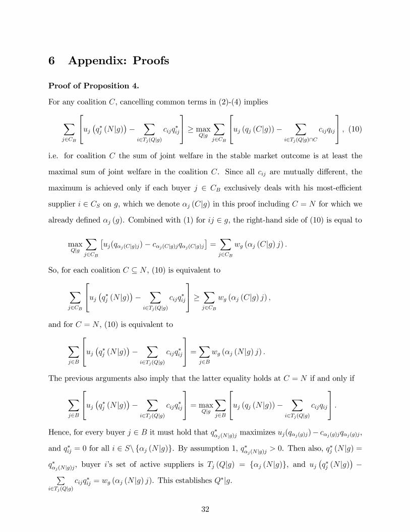
Proof of Proposition 4.

For any coalition C, cancelling common terms in (2)-(4) implies

∑j∈CB

uj (q∗j (N |g))−

∑i∈Tj(Q|g)

cijq∗ij

≥ maxQ|g

∑j∈CB

uj (qj (C|g))−∑

i∈Tj(Q|g)∩C

cijqij

, (10)i.e. for coalition C the sum of joint welfare in the stable market outcome is at least the

maximal sum of joint welfare in the coalition C. Since all cij are mutually different, the

maximum is achieved only if each buyer j ∈ CB exclusively deals with his most-effi cient

supplier i ∈ CS on g, which we denote αj (C|g) in this proof including C = N for which we

already defined αj (g). Combined with (1) for ij ∈ g, the right-hand side of (10) is equal to

maxQ|g

∑j∈CB

[uj(qαj(C|g)j)− cαj(C|g)jqαj(C|g)j

]=∑j∈CB

wg (αj (C|g) j) .

So, for each coalition C ⊆ N , (10) is equivalent to

∑j∈CB

uj (q∗j (N |g))−

∑i∈Tj(Q|g)

cijq∗ij

≥ ∑j∈CB

wg (αj (C|g) j) ,

and for C = N , (10) is equivalent to

∑j∈B

uj (q∗j (N |g))−

∑i∈Tj(Q|g)

cijq∗ij

=∑j∈B

wg (αj (N |g) j) .

The previous arguments also imply that the latter equality holds at C = N if and only if

∑j∈B

uj (q∗j (N |g))−

∑i∈Tj(Q|g)

cijq∗ij

= maxQ|g

∑j∈B

uj (qj (N |g))−∑

i∈Tj(Q|g)

cijqij

.Hence, for every buyer j ∈ B it must hold that q∗αj(N |g)j maximizes uj(qαj(g)j)− cαj(g)jqαj(g)j,

and q∗ij = 0 for all i ∈ S\ {αj (N |g)}. By assumption 1, q∗αj(N |g)j > 0. Then also, q∗j (N |g) =

q∗αj(N |g)j, buyer i’s set of active suppliers is Tj (Q|g) = {αj (N |g)}, and uj(q∗j (N |g)

)−∑

i∈Tj(Q|g)cijq

∗ij = wg (αj (N |g) j). This establishes Q∗|g.

32

Next, since trade takes place against prices P ∗|g, Q∗|g can be attained through such trade

if and only if p∗αj(N |g)j = cαj(N |g)j and p∗ij ≥ cij for all i ∈ S\ {αj (N |g)}. The last condition

in Definition 3 sets p∗ij = cij for every link with q∗ij = 0, and this is the case for every

i 6= αj (N |g). Since all cij are mutually different, p∗ij > cαj(N |g)j for all i ∈ S\ {αj (N |g)}.

Finally, we derive F ∗|g. Given Q∗|g, consider supplier i and his active customer network

Ti (Q∗|g), that is {i} ∪ Ti (Q∗|g). Suppose for ∈ Ti (Q

∗|g), that supplier i and part of

his trade network want to break away by excluding trade with buyer , that is consider

coalition C = {i} ∪ Ti (Q∗|g) \ {}. Given P ∗|g, supplier i’s producer surplus is equal to

f ∗i +∑

j∈Ti(Q∗|g)\{}f ∗ij. This implies that (2) is equivalent to

f ∗i +∑

j∈Ti(Q∗|g)\{}

[uj(q∗ij)− cijq∗ij

]= f ∗i +

∑j∈Ti(Q∗|g)\{}

wg (ij) .

Hence, (4) imposes

f ∗i +∑

j∈Ti(Q∗|g)\{}

wg (ij) ≥∑

j∈Ti(Q∗|g)\{}

wg (ij) ⇐⇒ f ∗i ≥ 0.

Given Q∗|g, consider buyer ∈ B, his second-effi cient supplier β (N |g), and this supplier’s

active customer network Tβ(N |g) (Q∗|g), that is C ={, β (N |g)

}∪ Tβ(N |g) (Q∗|g). Then,

(4) imposes

u(q∗α(N |g))− cα(N |g)q

∗i − f ∗α(N |g) +

∑j∈Tβ(N|g)(Q

∗|g)

wg (ij)

≥ wg(β (N |g)

)+

∑j∈Tβ(N|g)(Q

∗|g)

wg (ij) ,

Since u(q∗α(N |g))− cα(N |g)q∗i = wg (α (N |g) ), this condition is equivalent to

f ∗α(N |g) ≤ wg (α (N |g) )− wg(β (N |g)

)≤ wg (α (N |g) ) .

The prices p∗ij ≥ cij and the fees f ∗ij ≥ 0 for every link with q∗ij = 0 are unrestricted, and this

is the case for every i 6= αj (N |g). �

Proof of Proposition 6.

33

Given the history of proposed prices P |g, we define for each connected buyer j ∈ B the

lowest proposed price as pıj (P |g) = mini∈S:ij∈g {pij}, where ı denotes an arbitrary supplier

who set such lowest price (which might be αj (g)). Given history P |g, buyer j ∈ B purchases

qαj(g)j (P |g) =

{arg maxqαj(g)j≥0 uj(qαj(g)j)− pαj(g)jqαj(g)j, if pαj(g)j ≤ pıj (P |g) ,

0, otherwise,

qıj (P |g) =

{arg maxqıj≥0 uj(qıj)− pıjqıj, if pαj(g)j > pıj (P |g) ,0, otherwise,

qij (P |g) = 0, i 6= αj (g) , ı.

On the equilibrium path, ı = αj (g) or βj (g), buyer j purchases qαj(g)j(P |g) = qαj(g)j > 0

and qβj(g)j (P |g) = 0, which is in accordance to the endogenous tie-breaking rule in Simon

and Zame (1990). Verification that the suppliers’strategies and the buyers’strategies form a

subgame perfect equilibrium strategy profile goes as follows: On and offthe equilibrium path,

buyer j always purchases the optimal quantity from a supplier that offers the lowest price, so

his strategy is optimal for every history. If pαj(g)j = pMαj(g)j, then supplier αj (g)’s producer

surplus is maximal and this supplier does not want to deviate. If pαj(g)j = cβj(g)j, then

the deviation pαj(g)j > cβj(g)j implies that buyer j will exclusively trade with βj (g) against

the price pβj(g)j = cβj(g)j, and supplier αj (g) looses buyer j as his customer which reduces

his positive equilibrium profits on the link αj (g) j to zero. Also, the lower deviating price

pαj(g)j < pαj(g)j reduces supplier αj (g)’s profits. Hence, pαj(g)j is optimal given the other

strategies. Since the other suppliers do not trade whether or not they deviate by setting

other prices, they do not have any profitable deviating price. This establishes equilibrium.

There do not exist other Bertrand equilibrium outcomes. To see this, in any Bertrand

equilibrium buyers always purchase from suppliers who set the lowest price. For |Sj (g)| = 1,

αj (g) = 1 and standard monopoly pricing implies p1j = pM1j is the unique price. Next,

consider |Sj (g)| = 2. Renumber the suppliers in S such that Sj (g) = {1, 2}, αj (g) = 1

and βj (g) = 2. If pM1j < c2j, it is optimal for supplier 1 to act as a standard monopolist,

and supplier 2 would make negative profits by undercutting this price. Then, only p1j = pM1j

and any p2j ≥ c2j can be equilibrium prices. Next, pM1j ≥ c2j. Then, modification of the

34

arguments for the first-price auction with mutually different valuations in Simon and Zame

(1990), establishes that in any Bertrand equilibrium we must have p1j = p2j = c2j and buyer j

exclusively trades with supplier 1, i.e. q1j(P |g) = q1j and q2j(P |g) = 0. Finally, for |Sj (g)| ≥

3, it is straightforward to show that both pαj(g)j = pβj(g)j ≤ mini∈S\{αj(g),βj(g)}:ij∈g cij, and

then the arguments for |Sj (g)| = 2 apply to suppliers αj (g) and βj (g). The other pij ≥ cij

are unrestricted. �

Proof of Proposition 7.

Given the history h of proposed prices P |g and fees F |g, for each connected buyer j ∈ B

define the proposed price and fee combination from which this buyer can achieve the largest

consumer surplus as pıj (P |g) and fıj (P |g), where ı denotes an arbitrary supplier who set such

combination (which might be αj (g)). Given history h, buyer j ∈ B exclusively purchases

from supplier αj (g) the quantity qαj(g)j (h) = arg maxqαj(g)j≥0 uj(qαj(g)j)−pαj(g)jqαj(g)j−fαj(g)j

if

maxqαj(g)j≥0

uj(qαj(g)j)− pαj(g)jqαj(g)j − fαj(g)j ≥ maxi∈S:ij∈g

maxqij≥0

[uj(qij)− pijqij − fij] ,

and qαj(g)j (P |g) = 0 otherwise. Buyer j exclusively purchases from supplier ı the quantity

qıj (h) = arg maxqıj≥0 uj(qıj)− pıjqıj if

maxqαj(g)j≥0

uj(qαj(g)j)− pαj(g)jqαj(g)j − fαj(g)j < maxi∈S:ij∈g

maxqij≥0

[uj(qij)− pijqij − fij] ,

and qıj (P |g) = 0 otherwise. Buyer j always purchase qij (P |g) = 0 from the other suppliers.

On the equilibrium path, buyer j purchases q∗αj(g)j ≡ qαj(g)j(h∗), where history h∗ denotes

the proposed P ∗|g and F ∗|g. This is in accordance to the endogenous tie-breaking rule in

Simon and Zame (1990). Verification that the suppliers’strategies and the buyers’strategies

form a subgame perfect equilibrium strategy profile is as follows: For any history h on and

off the equilibrium path, buyer j always purchases the optimal quantity from one of the

suppliers from which he achieves the maximal consumer surplus dependent upon the history

h, so his strategy is optimal. Since p∗αj(g)j = cαj(g)j and f∗αj(g)j

= wg(αj (g) j)− wg(βj (g) j),

35

then any deviation pαj(g)j ≥ cαj(g)j and fαj(g)j ≥ f ∗αj(g)j with at least one strict inequality

implies that buyer j will exclusively trade with βj (g) against p∗βj(g)j = cβj(g)j and f∗βj(g)j

= 0,

and supplier αj (g) looses buyer j as his customer which reduces his equilibrium profit on the

link αj (g) j from f ∗αj(g)j > 0 to zero. Also, the lower deviating fee fαj(g)j < f ∗αj(g)j reduces

supplier αj (g)’s profits. Hence, p∗αj(g)j and f∗αj(g)j

are optimal given the other strategies.

Since the other suppliers do not trade independent of the prices and fees they set, there does

not exist any profitable deviating price and fee combination for any of them. This establishes

equilibrium.

There do not exist other equilibrium outcomes. To see this, in any equilibrium buyers

always purchase from suppliers who set a price and fee combination from which buyers can

achieve a maximal consumer surplus. For |Sj (g)| = 1, we renumber such that Sj (g) = {1}.

Since βj (g) = 0 and wg (0j) = 0, we have that p∗1j = c1j and f ∗1j = wg (1j) are optimal by

the results in Oi (1971). Next, consider |Sj (g)| = 2. Renumber the suppliers in S such that

Sj (g) = {1, 2}, αj (g) = 1 and βj (g) = 2. There cannot exist an equilibrium in which buyer

j exclusively trades with supplier 1 against p∗1j > c1j and

f ∗1j = maxq1j≥0

[uj(q1j)− p∗1jq1j

]− wg (2j) < wg (1j)− wg (2j) ,

because then supplier 1 can increase his profits arbitrarily close to wg (1j)−wg (2j) by setting

the deviating price p1j = c1j and f1j = wg (1j) − wg (2j) − ε, for suffi ciently small ε > 0.

So, in any equilibrium, supplier 1 can secure wg (1j) − wg (2j). Also, an equilibrium with

p∗1j > c1j and f ∗1j > maxq1j≥0[uj(q1j)− p∗1jq1j

]− wg (2j) is impossible. So, p∗1j = c1j in any

equilibrium. Next, there cannot exist an equilibrium with p∗2j > c2j and f ∗2j = 0 either. To

see this, first note that then buyer j would exclusively trade with supplier 1 against p∗1j = c1j

and

f ∗1j = wg (1j)−maxq2j≥0

[uj(q2j)− p∗2jq2j

]> wg (1j)− wg (2j) .

Exclusive trade is dictated by the insights in Simon and Zame (1990). Supplier 2 will

have a profit of zero, and could obtain a positive profit by setting p2j = c2j and f2j =

36

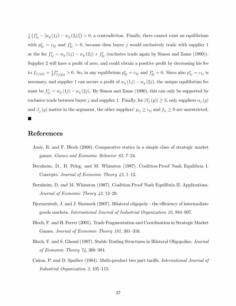
12

(f ∗1j − [wg (1j)− wg (2j)]

)> 0, a contradiction. Finally, there cannot exist an equilibrium

with p∗2j = c2j and f ∗2j > 0, because then buyer j would exclusively trade with supplier 1

at the fee f ∗1j = wg (1j) − wg (2j) + f ∗2j (exclusive trade again by Simon and Zame (1990)).

Supplier 2 will have a profit of zero, and could obtain a positive profit by decreasing his fee

to fβj(g)j = 12f ∗βj(g)j > 0. So, in any equilibrium p∗2j = c2j and f ∗2j = 0. Since also p∗1j = c1j is

necessary, and supplier 1 can secure a profit of wg (1j)−wg (2j), the unique equilibrium fee

must be f ∗1j = wg (1j)−wg (2j). By Simon and Zame (1990), this can only be supported by

exclusive trade between buyer j and supplier 1. Finally, for |Sj (g)| ≥ 3, only suppliers αj (g)

and βj (g) matter in the argument, the other suppliers’pij ≥ cij and fij ≥ 0 are unrestricted.

�

References

Amir, R. and F. Bloch (2009). Comparative statics in a simple class of strategic market

games. Games and Economic Behavior 65, 7—24.

Bernheim, D., B. Peleg, and M. Whinston (1987). Coalition-Proof Nash Equilibria I.

Concepts. Journal of Economic Theory 42, 1—12.

Bernheim, D. and M. Whinston (1987). Coalition-Proof Nash Equilibria II. Applications.

Journal of Economic Theory 42, 13—29.

Bjornerstedt, J. and J. Stenneck (2007). Bilateral oligopoly - the effi ciency of intermediate

goods markets. International Journal of Industrial Organization 25, 884—907.

Bloch, F. and H. Ferrer (2001). Trade Fragmentation and Coordination in Strategic Market

Games. Journal of Economic Theory 101, 301—316.

Bloch, F. and S. Ghosal (1997). Stable Trading Structures in Bilateral Oligopolies. Journal

of Economic Theory 74, 368—384.

Calem, P. and D. Spulber (1984). Multi-product two part tariffs. International Journal of

Industrial Organization 2, 105—115.

37

Camina, E. (2006). A generalized assignment game. Mathematical Social Sciences 52,

152—161.

Crouzeix, J.-P. and P. Lindberg (1986). Additively decomposed quasiconvex functions.

Mathematical Programming 35, 42—57.

Dana, J. (2012). Buyer groups and strategic commitments. Games and Economic Behav-

ior 74, 470—485.

Economides, N. (1986). Nash equilibrium in duopoly with products defined by two char-

acteristics. Rand Journal of Economics 17, 431—439.

Funaki, Y., H. Houba, and E. Motchenkova (2012). Market power in Bilateral Oligopoly

markets with Expandable Infrastructures. Working Paper, VU University Amsterdam,

mimeo.

Galbraith, J. (1952). American Capitalism: The concept of countervailing power. New

Brunswick, NJ, and London: Classics in Economics Series.

Harrison, M. and J. Kline (2001). Quantity competition with access fees. International

Journal of Industrial Organization 19, 345—373.

Hotelling, H. (1929). Stability in competition. Economic Journal 39, 41—57.

Inderst, R. and C. Wey (2007). Buyer power and supplier incentives. European Economic

Review 51, 647—667.

Jackson, M. (2005). Allocation rules for network games. Games and Economic Behav-

ior 51, 128—154.

Kanemoto, Y. (2000). Price and quantity competition among heterogeneous suppliers

with two-part pricing: applications to clubs, local public goods, networks, and growth

controls. Regional Science and Urban Economics 30, 587—608.

Lustgarten, S. (1975). The impact of buyer concentration in manufacturing industries.

Review of Economic Statistics 57, 125—132.

Mas-Colell, A., M. Whinston, and J. Green (1995).Microeconomic theory. Oxford: Oxford

University Press.

38

Motta, M. (2004). Competition Policy: Theory and Practice. Cambridge: Cambridge Uni-

versity Press.

Oi, W. (1971). A Disneyland dilemma: two-part tariffs for a Mickey Mouse monopoly.

Quarterly Journal of Economics 85, 77—96.

Roth, A. and M. Sotomayor (1990). Two-Sided Matching: A Study in Game-Theoretic

Modeling and Analysis. Cambridge: Cambridge University Press.

Salop, S. (1979). Monopolistic competition with outside goods. Bell Journal of Eco-

nomics 10, 141—156.

Scherer, F. and D. Ross (1990). Industrial market structure and economic performance

(3rd edition). Boston: Houghton Miffl in.

Schmalensee, R. (1981). Output and welfare implications of monopolistic third-degree

price discrimination. American Economic Review 71, 242—247.

Schmalensee, R. (1982). Monopolistic two-part pricing arrangements. Bell Journal of Eco-

nomics 12, 445—446.

Schumacher, U. (1991). Buyer structure and seller performance in U.S. manufacturing

industries. Review of Economic Statistics 73, 277—284.

Shapley, L. and M. Shubik (1972). The assignment game i: The core. International Journal

of Game Theory 1, 111—130.

Shapley, L. and M. Shubik (1977). Trade using one commodity as a means of payment.

Journal of Political Economy 85, 937—968.

Simon, L. andW. Zame (1990). Discontinuous games and endogenous sharing rules. Econo-

metrica 58, 861—872.

Sozanski, T. (2006). On the core of characteristic function games associated with exchange

networks. Social Networks 28, 397—426.

Tirole, J. (1988). The theory of industrial organization. London: MIT Press.

39