Market Preferences and Process Selection (MAPPS):

the Value of Perfect Flexibility

Stephen LawrenceUniversity of Colorado

George MonahanUniversity of Illinois

Tim SmuntWake Forest University

This research was partially funded by a College of BusinessCompetitive Summer Research Grant in Entrepreneurship

Objectives of Research

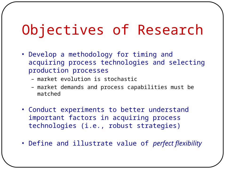
• Develop a methodology for timing and acquiring process technologies and selecting production processes– market evolution is stochastic

– market demands and process capabilities must be matched

• Conduct experiments to better understand important factors in acquiring process technologies (i.e., robust strategies)

• Define and illustrate value of perfect flexibility

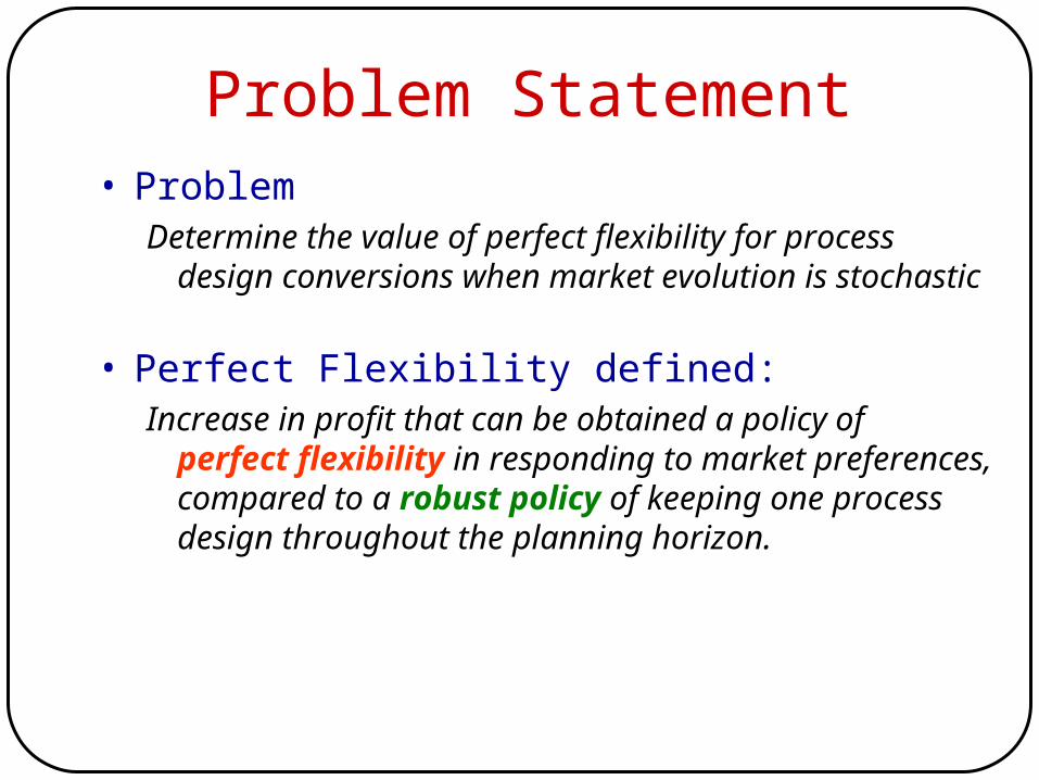
Problem Statement• Problem

Determine the value of perfect flexibility for process design conversions when market evolution is stochastic

• Perfect Flexibility defined:Increase in profit that can be obtained a policy of

perfect flexibility in responding to market preferences, compared to a robust policy of keeping one process design throughout the planning horizon.

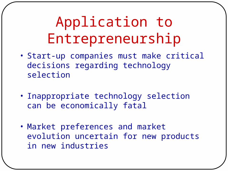
Application to Entrepreneurship

• Start-up companies must make critical decisions regarding technology selection

• Inappropriate technology selection can be economically fatal

• Market preferences and market evolution uncertain for new products in new industries

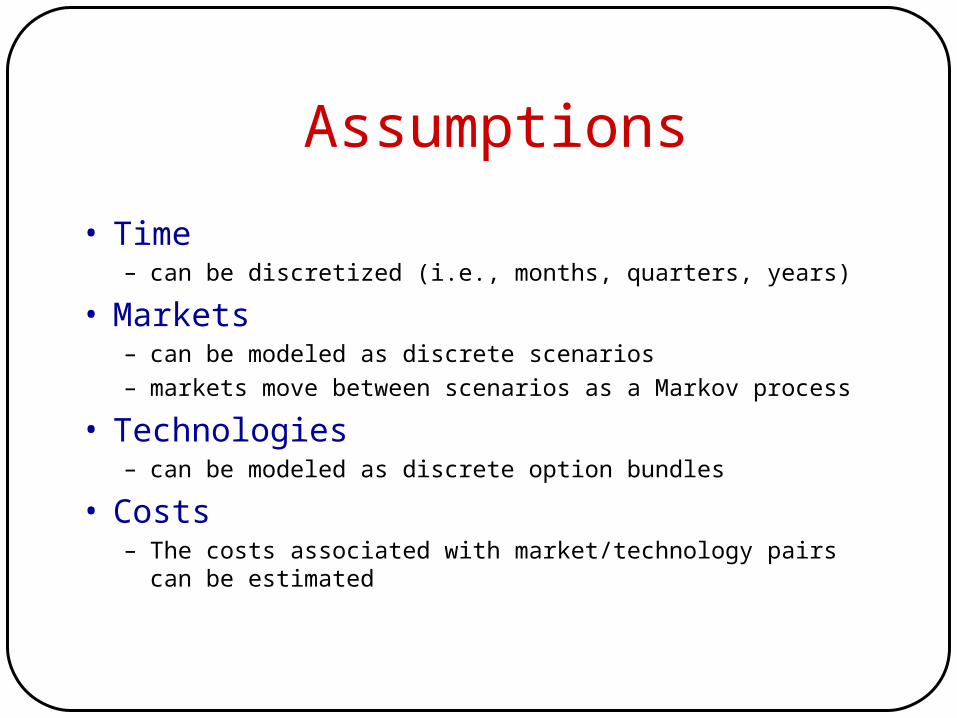
Assumptions

• Time – can be discretized (i.e., months, quarters, years)

• Markets – can be modeled as discrete scenarios

– markets move between scenarios as a Markov process

• Technologies– can be modeled as discrete option bundles

• Costs– The costs associated with market/technology pairs can be

estimated

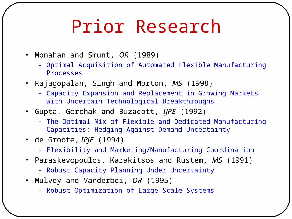
Prior Research

• Monahan and Smunt, OR (1989)– Optimal Acquisition of Automated Flexible Manufacturing Processes

• Rajagopalan, Singh and Morton, MS (1998)– Capacity Expansion and Replacement in Growing Markets with Uncertain

Technological Breakthroughs

• Gupta, Gerchak and Buzacott, IJPE (1992)– The Optimal Mix of Flexible and Dedicated Manufacturing Capacities:

Hedging Against Demand Uncertainty

• de Groote, IPJE (1994)– Flexibility and Marketing/Manufacturing Coordination

• Paraskevopoulos, Karakitsos and Rustem, MS (1991)– Robust Capacity Planning Under Uncertainty

• Mulvey and Vanderbei, OR (1995)– Robust Optimization of Large-Scale Systems

Solution Methodology

• Stochastic dynamic programming

• MAPPS – Market Preferences and Process Selection

A Simple Example

Market RequirementsHigh Variety Moderate Variety Standardized

Pro

cess

Cap

abil

itie

s HighFlexibility

ModerateFlexibility

StandardizedProduction

Job Shop

Batch Shop

Flow Shop

Hayes and Wheelwright, “The dynamics of process-product life cycles,” Harvard Business Review, March-April 1979

Flexible Shop

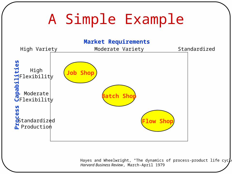
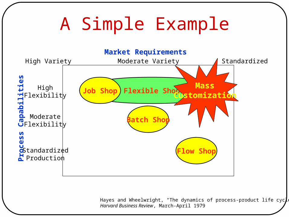
A Simple Example

Market RequirementsHigh Variety Moderate Variety Standardized

Pro

cess

Cap

abil

itie

s HighFlexibility

ModerateFlexibility

StandardizedProduction

Job Shop

Batch Shop

Flow Shop

Hayes and Wheelwright, “The dynamics of process-product life cycles,” Harvard Business Review, March-April 1979

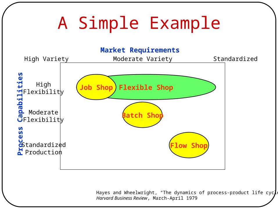
Flexible Shop

A Simple Example

Market RequirementsHigh Variety Moderate Variety Standardized

Pro

cess

Cap

abil

itie

s HighFlexibility

ModerateFlexibility

StandardizedProduction

Job Shop

Batch Shop

Flow Shop

Hayes and Wheelwright, “The dynamics of process-product life cycles,” Harvard Business Review, March-April 1979

MassCustomization

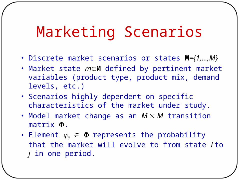
Marketing Scenarios

• Discrete market scenarios or states M={1,…,M}

• Market state mM defined by pertinent market variables (product type, product mix, demand levels, etc.)

• Scenarios highly dependent on specific characteristics of the market under study.

• Model market change as an M M transition matrix .

• Element ij represents the probability that the market will evolve to from state i to j in one period.

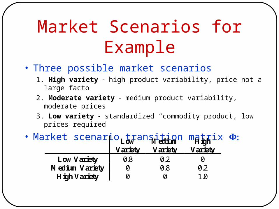
Market Scenarios for Example

• Three possible market scenarios1. High variety high product variability, price not a large facto

2. Moderate variety medium product variability, moderate prices

3. Low variety standardized “commodity product, low prices required

• Market scenario transition matrix

LowVariety

MediumVariety

HighVariety

Low Variety 0.8 0.2 0Medium Variety 0 0.8 0.2

High Variety 0 0 1.0

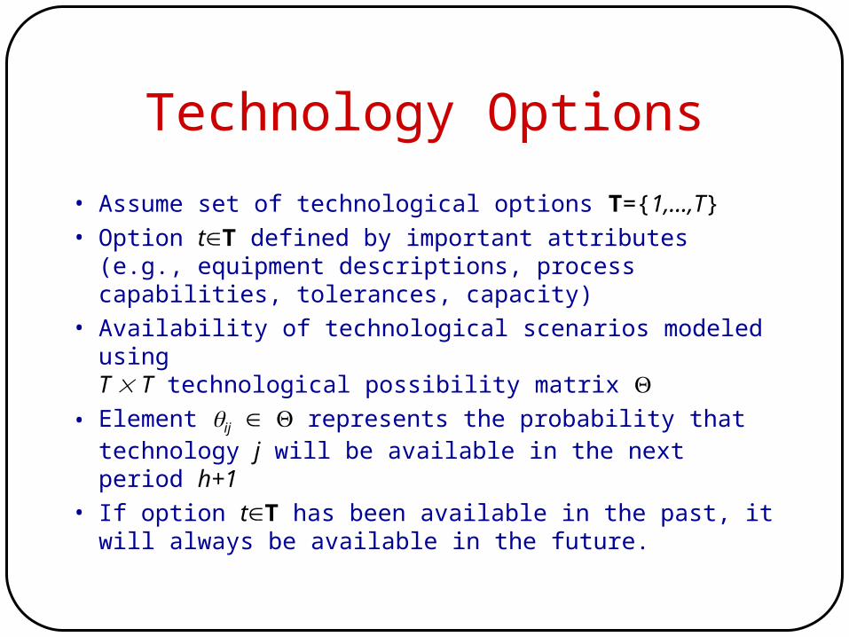
Technology Options

• Assume set of technological options T={1,…,T}

• Option tT defined by important attributes (e.g., equipment descriptions, process capabilities, tolerances, capacity)

• Availability of technological scenarios modeled usingT T technological possibility matrix

• Element ij represents the probability that technology j will be available in the next period h+1

• If option tT has been available in the past, it will always be available in the future.

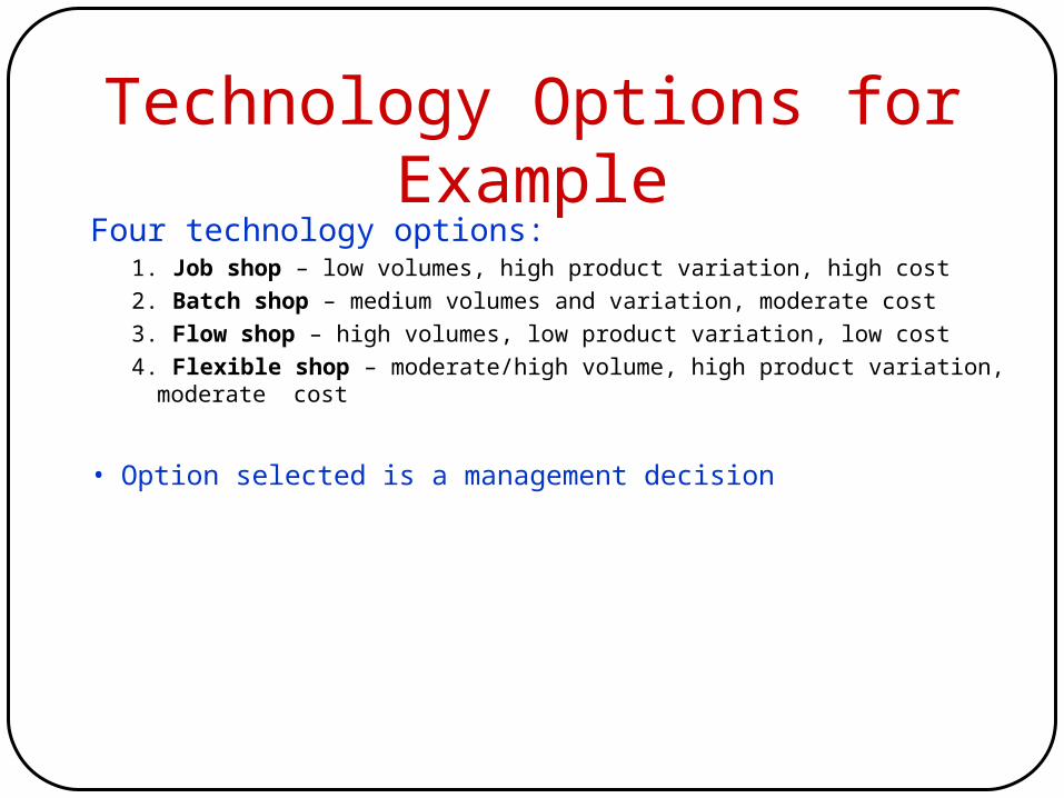
Technology Options for ExampleFour technology options:

1. Job shop – low volumes, high product variation, high cost

2. Batch shop – medium volumes and variation, moderate cost

3. Flow shop – high volumes, low product variation, low cost

4. Flexible shop – moderate/high volume, high product variation, moderate cost

• Option selected is a management decision

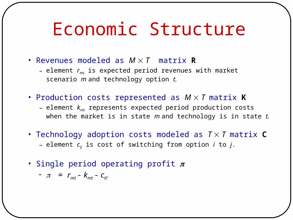
Economic Structure

• Revenues modeled as M T matrix R – element rmt is expected period revenues with market scenario m and technology

option t.

• Production costs represented as M T matrix K – element kmt represents expected period production costs when the market is in

state m and technology is in state t.

• Technology adoption costs modeled as T T matrix C– element cij is cost of switching from option i to j.

• Single period operating profit = rmt - kmt - ctt’

Revenue & Production Costs for Example

• Revenue matrix R

• Production cost matrix K

JobShop

BatchShop

FlowShop

FlexibleShop

Low Variety 100 100 100 100Medium Variety 125 500 600 800

High Variety 150 600 1,000 1,200

JobShop

BatchShop

FlowShop

FlexibleShop

Low Variety 75 100 400 300Medium Variety 75 400 500 650

High Variety 75 400 750 800

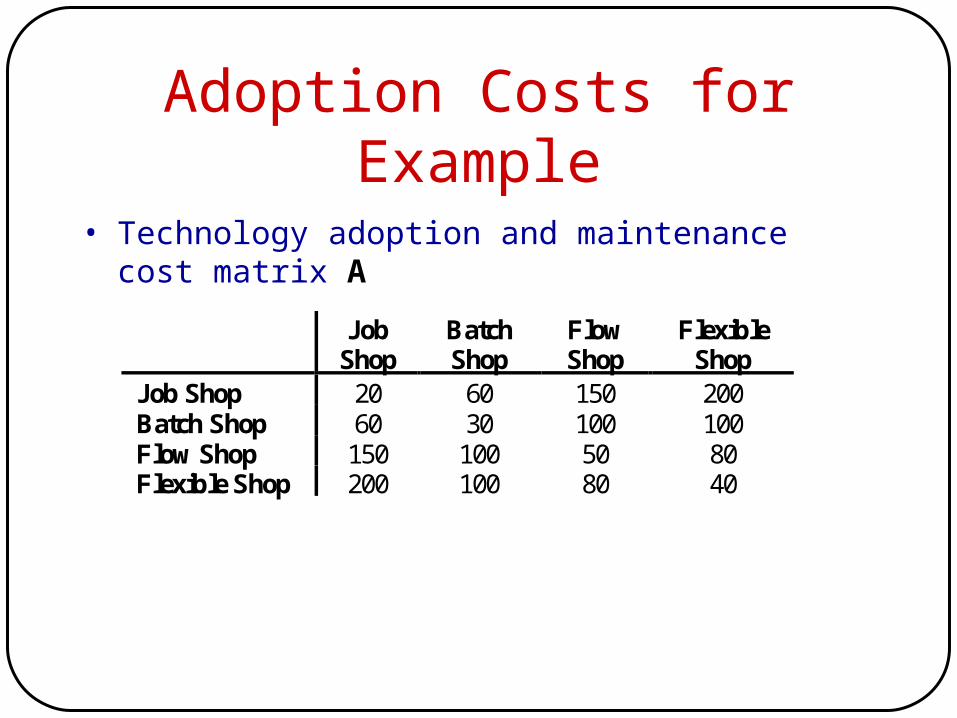
Adoption Costs for Example

• Technology adoption and maintenance cost matrix A

JobShop

BatchShop

FlowShop

FlexibleShop

Job Shop 20 60 150 200Batch Shop 60 30 100 100Flow Shop 150 100 50 80Flexible Shop 200 100 80 40

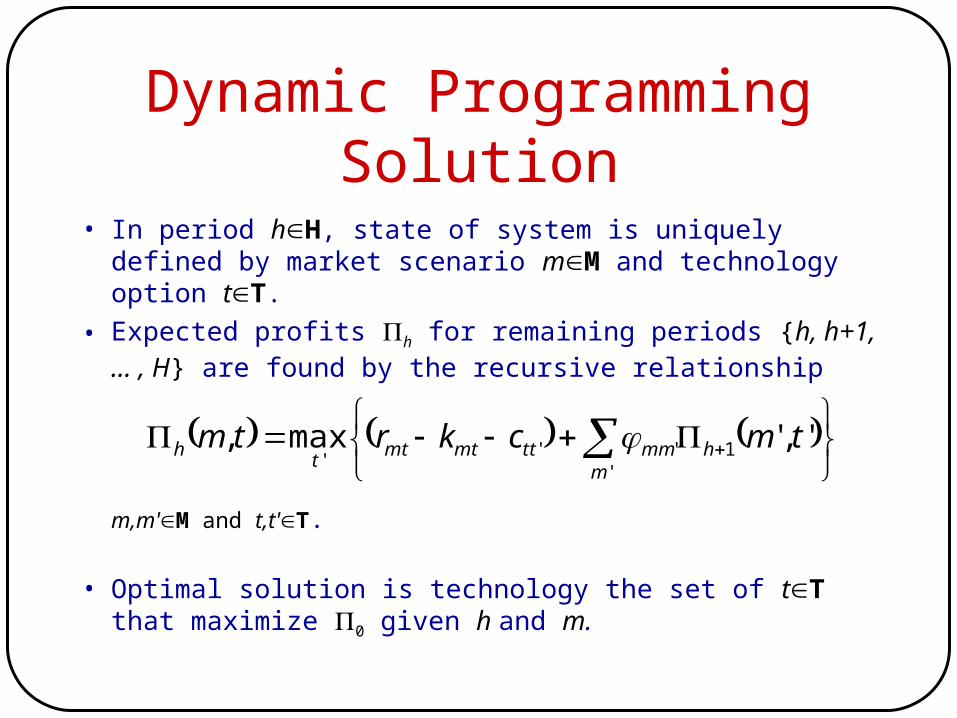
Dynamic Programming Solution

• In period hH, state of system is uniquely defined by market scenario mM and technology option tT.

• Expected profits h for remaining periods {h, h+1, … , H} are found by the recursive relationship

m,m'M and t,t'T.

• Optimal solution is technology the set of tT that maximize 0 given h and m.

'

1'''

','max,m

hmmttmtmtt

h tmckrtm

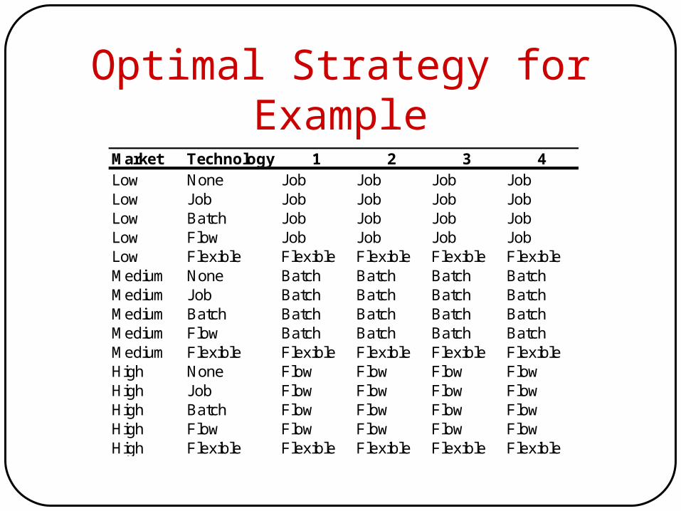
Optimal Strategy for ExampleMarket Technology 1 2 3 4Low None Job Job Job JobLow Job Job Job Job JobLow Batch Job Job Job JobLow Flow Job Job Job JobLow Flexible Flexible Flexible Flexible FlexibleMedium None Batch Batch Batch BatchMedium Job Batch Batch Batch BatchMedium Batch Batch Batch Batch BatchMedium Flow Batch Batch Batch BatchMedium Flexible Flexible Flexible Flexible FlexibleHigh None Flow Flow Flow FlowHigh Job Flow Flow Flow FlowHigh Batch Flow Flow Flow FlowHigh Flow Flow Flow Flow FlowHigh Flexible Flexible Flexible Flexible Flexible

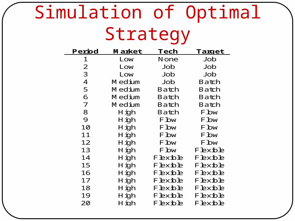
Simulation of Optimal StrategyPeriod Market Tech Target

1 Low None Job2 Low Job Job3 Low Job Job4 Medium Job Batch5 Medium Batch Batch6 Medium Batch Batch7 Medium Batch Batch8 High Batch Flow9 High Flow Flow10 High Flow Flow11 High Flow Flow12 High Flow Flow13 High Flow Flexible14 High Flexible Flexible15 High Flexible Flexible16 High Flexible Flexible17 High Flexible Flexible18 High Flexible Flexible19 High Flexible Flexible20 High Flexible Flexible

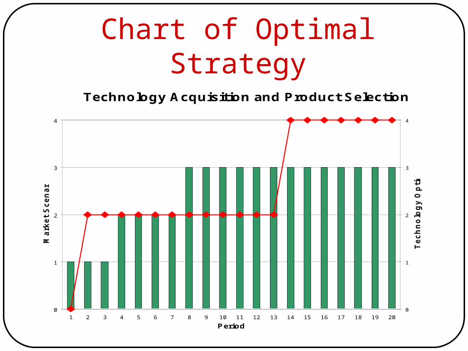
Chart of Optimal Strategy

Technology Acquisition and Product Selection

0

1

2

3

4

1 2 3 4 5 6 7 8 9 10 11 12 13 14 15 16 17 18 19 20

Period

Ma

rke

t S

ce

na

rio

0

1

2

3

4

Te

ch

no

log

y O

pti

on

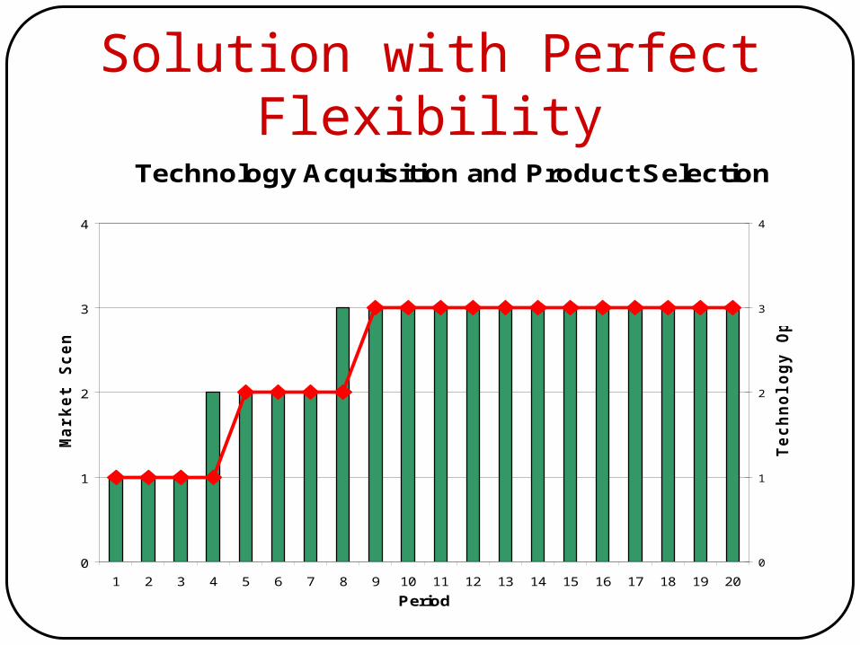
Solution with Perfect Flexibility

Technology Acquisition and Product Selection

0

1

2

3

4

1 2 3 4 5 6 7 8 9 10 11 12 13 14 15 16 17 18 19 20

Period

Ma

rke

t S

ce

na

rio

0

1

2

3

4

Te

ch

no

log

y O

pti

on

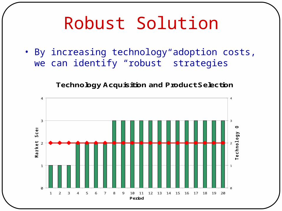
Robust Solution

• By increasing technology adoption costs, we can identify “robust” strategies

Technology Acquisition and Product Selection

0

1

2

3

4

1 2 3 4 5 6 7 8 9 10 11 12 13 14 15 16 17 18 19 20

Period

Ma

rke

t S

ce

na

rio

0

1

2

3

4

Te

ch

no

log

y O

pti

on

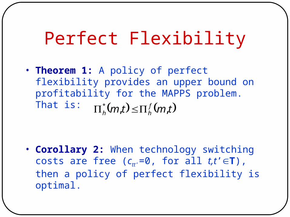
Perfect Flexibility

• Theorem 1: A policy of perfect flexibility provides an upper bound on profitability for the MAPPS problem. That is:

• Corollary 2: When technology switching costs are free (ctt’=0, for all t,t’T), then a policy of perfect flexibility is optimal.

tmtm fhh ,,*

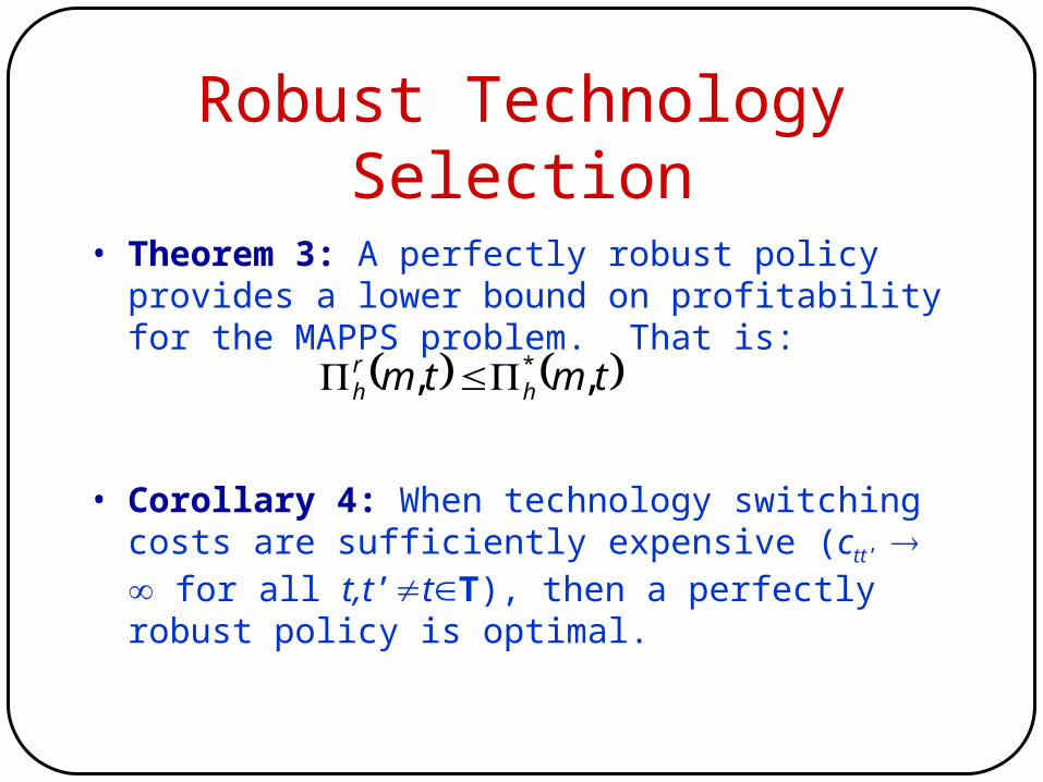
Robust Technology Selection

• Theorem 3: A perfectly robust policy provides a lower bound on profitability for the MAPPS problem. That is:

• Corollary 4: When technology switching costs are sufficiently expensive (ctt’ for all t,t’tT), then a perfectly robust policy is optimal.

tmtm hrh ,, *

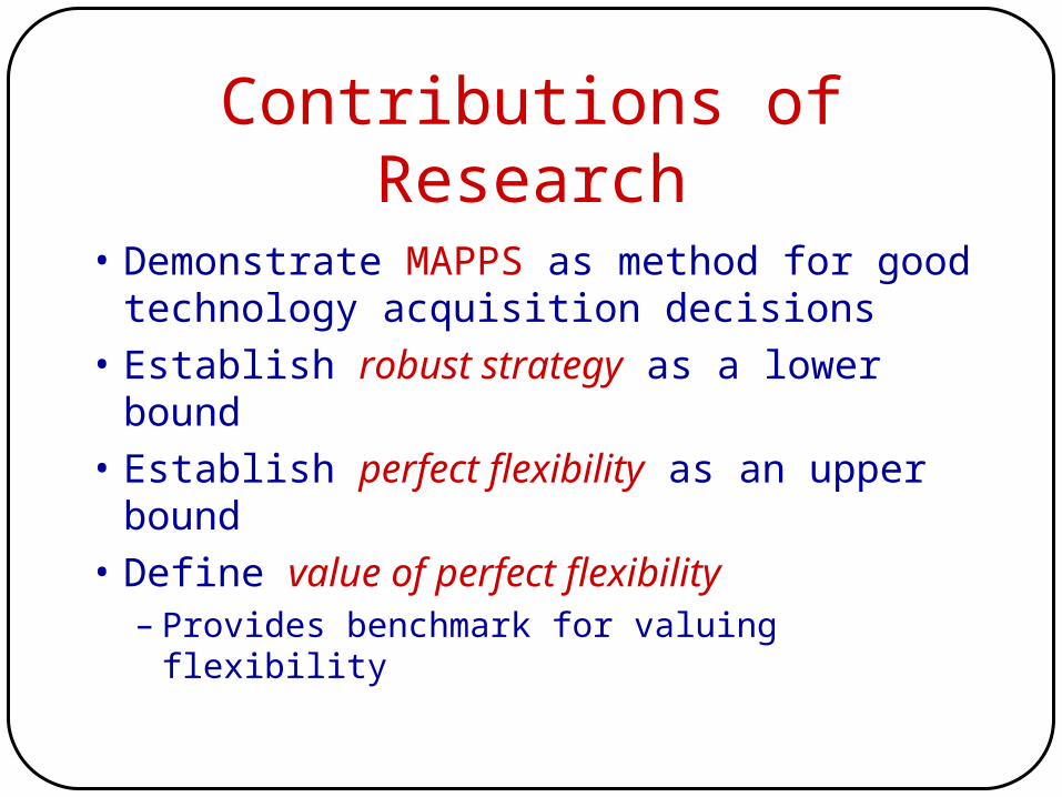
Contributions of Research

• Demonstrate MAPPS as method for good technology acquisition decisions

• Establish robust strategy as a lower bound

• Establish perfect flexibility as an upper bound

• Define value of perfect flexibility– Provides benchmark for valuing flexibility

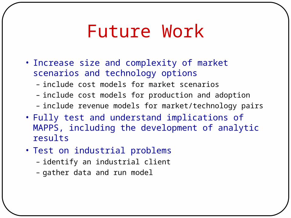
Future Work

• Increase size and complexity of market scenarios and technology options– include cost models for market scenarios– include cost models for production and adoption– include revenue models for market/technology pairs

• Fully test and understand implications of MAPPS, including the development of analytic results

• Test on industrial problems– identify an industrial client– gather data and run model

Some other examples...

Questions?

Market Preferences and Process Selection (MAPPS):

the Value of Perfect Flexibility