Market Structure, Oligopsony Power, and Productivity

Michael Rubens*

February 27, 2021

Abstract

I study how ownership consolidation affects market power on both factor andproduct markets, and productivity. I develop a model to separately identify markups,markdowns and productivity using production and cost data. I use the model toexamine the effects of a large-scale consolidation wave in the Chinese cigarettemanufacturing industry. I find that this consolidation led to an increase in inter-mediate input price markdowns of 30%, but to a slight drop in cigarette pricemarkups. Although the consolidation was defended as a means to spur produc-tivity growth, I find that it actually lowered aggregate productivity.

Keywords: Market Power, Oligopsony, Productivity, Concentration

JEL Codes: L10, J42, O25, D33

*KU Leuven and Research Foundation Flanders. E-mail: michael.rubens@kuleuven.be.This paper previously circulated under the title ‘Ownership consolidation, monopsony power and ef-ficiency: Evidence from the Chinese tobacco industry’. I am grateful to Jan De Loecker and Jo VanBiesebroeck for their advice. I also thank Frank Verboven, Chad Syverson, Otto Toivanen, Dan Acker-berg, Myrto Kalouptsidi, Mingzhi Xu, and Benjamin Vatter for helpful suggestions, and participants atvarious conferences and workshops. Financial support from the Research Foundation Flanders (Grant11A4618N), Fulbright Belgium and the Belgian American Educational Foundation is gratefully ac-knowledged.

1 IntroductionThere is an ongoing debate about the aggregate evolution of market concentration and market

power, both in the U.S.A. and at a global level (Rossi-Hansberg et al., 2018; Autor et al., 2017;

Covarrubias et al., 2020; De Loecker et al., 2020). Increasing market concentration can lead to

changes in productive efficiency due to scale economies and returns to scale, but can also affect

both oligopoly power of firms on their product markets, and oligopsony power on their input

markets. Existing empirical work on the consequences of changing market concentration and

ownership consolidation typically focuses on a subset of these three effects, while assuming away

the others.

This paper fills this gap by empirically examining the joint effects of ownership consolidation

on product price markups, input price markdowns, and total factor productivity. For this pur-

pose, I construct a structural model to separately identify the markup, which is the wedge between

marginal costs and product prices, the markdown, which is the wedge between marginal costs and

input prices, and total factor productivity. I build on the ‘cost-side’ approach to markup identifi-

cation of Hall (1986) and De Loecker and Warzynski (2012), which has been extended to allow

for endogenous input prices by De Loecker et al. (2016) and Morlacco (2017). I show that this

class of models, which imposes only a model of production and input demand, fails to separately

identify markups and markdowns as soon as a subset of inputs is non-substitutable.1 This is often

the case for intermediate inputs in industries such as beer brewing (hop), coffee roasting (beans)

and consumer electronics (rare earth metals), among many others.2 I solve this identification chal-

lenge by combining the input demand conditions that are derived from the production model with

an input supply model. I rely on a discrete choice model of input suppliers choosing differentiated

manufacturers in the spirit of Berry (1994). I make use of input demand shocks from the estimated

production model to help identify the input supply function.

I use this model to study how a large-scale consolidation wave in the Chinese cigarette manu-

facturing industry affected markups, markdowns and productive efficiency. This industry provides

1In their analysis of market power in the beer industry, De Loecker and Scott (2016) also allowed for a non-substitutableinput, but not for input market power.

2Even if intermediate inputs are substitutable to a limited extent, the implications of this paper still matter. Markdownsand markups would then be weakly identified, rather than non-identified.

1

a particularly interesting setting because the consolidation was the result of a government pol-

icy that forced manufacturers below certain production thresholds to exit the market after 2002.

This allows comparing firms with and without competitors below the exit thresholds before and

after 2002. A legal prohibition to transport tobacco leaf across local markets ensures that these

markets are isolated, and can hence be considered as treatment and control groups. Such quasi-

experimental variation in market structure is rare, and very useful because other sources of market

structure variation, such as mergers and acquisitions and organic exit and entry, tend to be en-

dogenous to both productivity and market power.3 That being said, the identification approach for

markups, markdowns and productivity is generally applicable outside of this particular industry.

The key driver of oligopsony power on Chinese leaf markets is the legal obligation of tobacco

farmers to sell their entire output locally, which restricts their choice set of potential buyers. More-

over, crop switching costs and legal restrictions on migration and land use make the outside option

of quitting tobacco farming less attractive. These kinds of frictions characterize rural labor mar-

kets in most of the developing world, so the evidence for oligopsony power found in this paper is

likely to apply to other industries and countries as well.4 The structure of the tobacco value chain

is, moreover, particularly conducive to oligopsony power: around 8 million farmers sell leaves to

manufacturers, of which the number decreased from 350 to 150 during the consolidation. These

manufacturers in turn sell cigarettes to a monopsonistic government-controlled wholesaler.5

The analysis is structured in four main parts. I start by providing evidence for the effects of

the consolidation on both input and product prices. I find that leaf prices at firms in consolidated

markets fell by 34% compared to the other firms after 2002. Factory-gate cigarette prices fell as

well, by 21% on average. Employee wages did, however, not change significantly. This suggests

that the consolidation affected competition on leaf markets and labor markets differently. The

reduced-form evidence alone does not suffice, however, to draw conclusions about the underlying

mechanism: input and product prices could have changed due to changes in productive efficiency,

3Beside this feature, this industry is also interesting due to its mere size: annual industry revenue exceeds $7 billion, and40% of the world’s cigarettes are made in China. Moreover, public health externalities are obviously an idiosyncraticaspect of the tobacco industry, although I will abstract from these in the paper.

4Localized agricultural markets due to internal trade regulations are, for instance, a driver of oligopsony power onIndian agricultural markets (Chatterjee, 2019), and switching costs are key in the agricultural economics literature(Song et al., 2011).

5The tobacco industry remained largely domestic even after China’s WTO accession, as exports make up for less than1% of industry revenue. This eliminates various potentially confounding factors which relate to international trade.

2

oligopsony power, and/or product market power.

I therefore continue by constructing and estimating a structural model to recover cigarette price

markups, leaf price markdowns, and total factor productivity of manufacturing firms. I find that

markups were not significantly different from one, meaning that the prices of cigarettes were equal

to their marginal costs. Leaf price markdowns were, in contrast, large: the median cigarette man-

ufacturer paid its tobacco farmers merely a fourth of their marginal revenue product, which is

a similar wedge compared to prior work on China. The combination of low markups and high

markdowns implies that manufacturers mainly had market power on their intermediate input mar-

kets, which is consistent with the fact that local leaf markets are concentrated, and farmers small,

whereas labor and cigarette markets are much less concentrated and not subject to the same fric-

tions.6

Next, I use the model estimates to examine the effects of the ownership consolidation. I find

that the consolidation policy led to increased oligopsony power on leaf markets: leaf price mark-

downs of firms in the treatment group increased on average by 30% compared to the control group

between 2002 and 2006. Cigarette price markups fell, however, which I rationalize using a bar-

gaining model of the wholesale market with double marginalization. I find, finally, no evidence

for average manufacturing productivity to have increased as a result of the consolidation, despite

this being the main official motivation for enforcing the size restrictions. Aggregate productivity

even fell by 23% due to the consolidation, as oligopsony power leads to input misallocation, just

as oligopoly power does (Edmond et al., 2018; Asker et al., 2019).

Finally, I use the model to quantify the extent to which the consolidation contributed to rural-

urban income inequality in the tobacco industry. Many papers have been devoted to this margin of

inequality in China, as it has increased rapidly since the early 1990s (Yang, 1999; Ravallion and

Chen, 2009). By increasing markdowns on tobacco leaf markets, but not on manufacturing labor

markets, income inequality between rural farmers and urban manufacturing workers increased by

twice as much as it would have without the consolidation.7

6High markdowns are also consistent with widespread poverty among Chinese tobacco farmers, in contrast to mostother tobacco-growing countries where tobacco ranks high among crops in terms of profitability (FAO, 2003).

7This surge in rural-urban inequality was not in line with official policy objectives, as laid out in President Hu Jintao’sHarmonious Society program during the mid-2000s. In 2017, the 13th five-year plan introduced targeted subsidiesto alleviate poverty among tobacco farmers. Such transfer schemes may not have been necessary in the absence of aconsolidation.

3

The key contribution of this paper is to examine how changes in market structure affect both

product price markups, input price markdowns and productivity. A secondary contribution is that I

develop an empirical framework that separately identifies these three variables even if not all inputs

are substitutable. The paper relates to two different strands of literature. First, I contribute to the

literature on the effects of ownership consolidation and increasing market concentration. Papers

that study the effects of ownership consolidation on productivity, such as Braguinsky et al. (2015)

and Grieco et al. (2017), and on market power, such as Nevo (2001) and Miller and Weinberg

(2017), among many others, typically assume that input prices are exogenous to firms. Prager and

Schmitt (2021) is an exception which does study the input market effects of mergers, and finds that

hospital mergers lead to slower wage growth when mergers are large and worker skills industry-

specific. In general, however, such wage changes can be caused by both changes in productivity,

markups, and/or markdowns. I therefore contribute to this literature by allowing both markups,

markdowns, and productivity to change in response to ownership consolidation.

Allowing for market power on both product and input markets is crucial to fully understand

the competitive effects of ownership consolidation. If one would solely focus on cigarette price

markups, the modest drop in these markups would lead to the conclusion that the consolidation was

pro-competitive. In reality, total market power rose due to an even larger increase in input price

markdowns. Moreover, allowing for oligopsonistic input markets is important when evaluating

often-made claims that mergers and acquisitions increase productive efficiency. As input prices and

quantities are usually not separately observed in production and cost data sets, assuming exogenous

input prices leads to an overestimation of the productivity gains from ownership consolidation if

there is oligopsony power, because falling input prices are erroneously interpreted as increased

efficiency. This has implications beyond traditional competition policy. Large-scale government-

initiated industry consolidation programs, such as the one studied in this paper, are becoming

increasingly popular in countries such as China and Indonesia. China recently consolidated, for

instance, many of its state-owned enterprises (SOEs) into industrial giants in various important

industries such as energy, transport utilities, telecommunication and military equipment.8 The

prior literature found such policies to generally increase productivity, but this could just as well be

8These policies are also known as “Grasping the large and letting the small go” (Naughton, 2007).

4

due to increased oligopsony power, which has the opposite effect on economic growth.9

A second related literature focuses on the identification of oligopsony power. Two broad classes

of models exist. A first approach is to identify both markups and markdowns using a production

approach by comparing input demand conditions across inputs, as done by Morlacco (2017) and

Brooks et al. (2021). A second approach is to impose a model of input supply and competition

on input markets. A recent literature has used discrete choice models of input supply with differ-

entiated firms to model labor market power, such as Card et al. (2018), Azar et al. (2019), and

Lamadon et al. (2019).10 These papers focus, however, exclusively on input market competition,

and hence do not allow for markup heterogeneity. I bridge both approaches by combining a pro-

duction and cost model with an input supply model. This has the benefit over the ‘pure’ production

and cost models of not having to make the assumptions that all inputs are substitutable, and that at

least one flexible input has an exogenous price. It comes at the cost, however, of having to impose

more structural assumptions on how firms compete against each other on their input markets and

about the preferences of input suppliers.11 In contrast to the discrete choice models of oligopsony

power, I identify not only markdowns, but also markups and productivity. One exception which

also identifies markups and markdowns using an input supply model is Kroft et al. (2020) on the

U.S. construction industry, but it does not focus on ownership consolidation. It uses a different

methodology that relies on observing auction bids to estimate the pass-through rate from winning

a bid to input quantities and prices. I rely, in contrast, on a quantity production function and

pass-through rates from productivity shocks to input prices.

The remainder of this paper has the following structure: I discuss the industry setting, data, and

stylized facts in section 2. The model is presented in section 3, and estimated in section 4. I end

with discussing the aggregate consequences of ownership consolidation in section 5.

9Hsieh and Song (2015) find, for instance, that consolidation policies similar to the one studied in this paper led to anincrease in aggregate TFP of 20% across all Chinese manufacturing industries, and Chen et al. (2018) estimate thatprivatizations of SOEs lead to important productivity gains.

10I refer to Manning (2011) for an overview of the broader oligopsony literature. Other recent work on oligosony powerwith different research questions and modelling strategies include Naidu et al. (2016); Goolsbee and Syverson (2019);Berger et al. (2019); Jarosch et al. (2019).

11Tortarolo and Zarate (2018) also combine a production model with an input supply model, but with a different identi-fication strategy, assuming substitutable inputs, and with a different research question.

5

2 Key facts on the Chinese tobacco industry

2.1 Industry setting

Farming The value chain of the production of cigarettes in China is visualized in figure 1(a).

At the start of the panel in 1999, there were around 8 million tobacco farms in China, which

were mostly organized at the household level and operated small plots of around 0.3-0.4 ha (FAO,

2003). After being harvested and dried, tobacco leaf needs to be ‘cured’.12 Farmers sell cured

tobacco leaf to cigarette manufacturers through local ‘purchasing stations’. Before being sold,

tobacco leaves are sorted into quality ‘grades’, each of which sells at a different price. Farmers

are obliged to sell their leaf output at purchasing stations in their own county. Tobacco leaf cannot

be transported across county borders without the approval of the provincial board of the industry

regulator, the State Tobacco Monopoly Administration (STMA). Leaf markets are therefore in

theory restricted to the county-level.13 In practice, there is some tobacco trade across counties and

cigarette manufacturers frequently locate purchasing stations near county borders to attract nearby

farmers from other counties (Peng, 1996).

Chinese tobacco farms became less profitable during the time period of interest: being the

median cash crop in terms of farm profitability in 1997, tobacco leaf dropped to the last place in

2004. (FAO, 2003; Hu et al., 2006). Although tobacco farmers can switch to other crops, this

entails important switching costs. A policy intervention in which Chinese tobacco farmers were

helped to substitute crops in 2008 found that substituting increased annual revenue per acre by

21% to 110% (Li et al., 2012). The fact that farmers do not substitute despite these potential gains

are suggestive for large crop switching costs. Farmers can also exit agriculture altogether, but

rural emigration is constrained due to the Hukou registration system. Some sources also mention

coercion of tobacco farmers into not switching crops by local politicians, due to the importance

of tobacco for local fiscal revenue (Peng, 1996). Land tenure insecurity does, finally, also make

migration more costly. Because rural land is the property of villages or collectives, farmers lose

their exclusive land use rights when moving (Minale, 2018).

12Various alternative processes are possible, such air curing, fire curing and flue curing.13Source: Regulation for the Implementation of the Law on Tobacco Monopoly of the People’s Republic of China, State

Council of the People’s Republic of China (1997).

6

Figure 1: Tobacco industry structure

(a) Value chain

Farmers (8M)

Cigarette manufacturers (350 → 150)

Wholesaler (monopolist)

Retailers

Consumers

Tobacco leaf

Cigarettes

(b) Manufacturing locations in 1999

(c) Manufacturing locations in 2006

Notes: Panel (a) gives a schematic overview of the cigarette value chain in China. The manu-facturers, in bold, are the entities observed in this paper. “CNTTC” stands for Chinese NationalTobacco Trade Company, and is the wholesaling arm of the CNTC/STMA. This is a government-controlled monopolist. Panels (b)-(c) map the counties with at least one cigarette manufacturingfirm in 1999 and 2006. These counties contained on average 1.24 firms.

Manufacturing Cigarette manufacturers turn tobacco leaf and other intermediate inputs, such as

paper and filters, into cigarettes using labor and capital. Intermediate inputs make up for 90% of

variable input expenditure, which consists of labor and intermediate inputs. Tobacco leaf accounts

for around two thirds of intermediate input expenditure, so I will refer to intermediate inputs as

‘tobacco’ leaf for the remainder of the paper.14 Almost all Chinese cigarette manufacturers are

formally subsidiaries of the Chinese National Tobacco Corporation (CNTC). In practice, however,

they operate as separate enterprises responsible for their own losses and profits (Peng, 1996). They

14The Chinese data do not break down intermediate inputs into more detailed categories, but US census data from 1997show that tobacco leaves make up for for 60% of all intermediate input costs in tobacco manufacturing firms (U.S.Census Bureau, 1997). Other intermediate inputs, such as filters and paper, fit the assumptions made for tobacco leaf,as they are likely to be non-substitutable as well.

7

are autonomous in how they operate and set input prices and compete against each other (Wang,

2013). Maps of tobacco manufacturing locations in 1999 and 2006 are in figures 1(b)-(c).

Wholesaling Manufacturers sell their cigarettes to wholesalers which are controlled by the State

Tobacco Monopoly Administration (STMA) through its commercial counterpart, the Chinese Na-

tional Tobacco Trade Corporation (CNTTC).15 This organization is centrally controlled and op-

erates a monopoly on the cigarette market. In contrast to tobacco leaf, cigarette markets are not

isolated: they are sold outside their prefecture or province of origin.16 The distinction between cen-

trally controlled wholesaling and decentralized manufacturing has been at the core of the STMA

system since its inception in the early 1980s. Even after China joined the WTO in 2001, the Chi-

nese tobacco industry has been shielded from international competition. Industry-wide exports

and imports were merely 1.0% and 0.2% of total industry revenue between 1998 and 2007.17 The

fiscal importance of the tobacco industry may be an important reason for this protection: in 1997,

tobacco taxes and monopoly profits made up for 10.4% of central government revenue. In 2015,

tax revenues from the cigarettes industry amounted to ¥840 B, which is 6.2% of China’s total tax

revenue, according to the 2015 annual report of the State Administration of Taxation.

2.2 Data

I use production and cost data on the cigarette manufacturers between 1999 and 2006 from the An-

nual Survey of Industrial Firms (ASIF), which is conducted by the National Bureau for Statistics

(NBS). The above-scale survey includes non-SOEs with sales exceeding 5 million RMB and all

SOEs irrespective of their size.18 The unit of observation in the NBS data is the ‘establishment’,

which also includes subsidiaries. As was mentioned earlier, however, cigarette manufacturing es-

tablishments can be considered to be independent firms, and will therefore be referred to as ‘man-

ufacturing firms’ in the remainder of the paper. I retain all manufacturers in the sector “Tobacco

and Manufactured Tobacco Substitutes”, which includes cigar and cigarette substitute producers,

besides ‘pure’ cigarette producers. The product-level descriptions in the data show, however, that

15STMA and CNTTC share most of their leadership (Wang, 2013).16Source: Regulation for the Implementation of the Law on Tobacco Monopoly of the People’s Republic of China, State

Council of the People’s Republic of China (1997). Market shares are, however, larger in the home provinces ofproducers, which is probably due to both transportation costs and provincial home bias.

17Source: UN Comtrade, accessed at http://comtrade.un.org/.18I refer to Brandt et al. (2012) for a comprehensive discussion of this data set.

8

firms in the former categories often produce cigarettes as their main product as well, which is why

they are included, even if they represent less than 5% of total revenue. The resulting ASIF sample

consists of 470 firms and 2,025 observations.

I supplement the ASIF data with production quantity data at the product-firm-month level dur-

ing the same time period, which is collected by the NBS as well. Quantities are observed for a

subset of 1,260 observations and 274 firms.19 Combining both data sets and cleaning the data

reduces the sample size to 1,120 observations and 254 firms, which covers 80% of total revenue

in the raw data.20 I also obtain population statistics from the 2000 census and obtain brand-level

cigarette characteristics on a subset of firms for some robustness checks.21

Leaf market definitions Because of the legal leaf trade restrictions, I define leaf markets at the

prefecture level. There were on average 1.9 cigarette manufacturers per prefecture throughout

the sample, and 193 prefectures with at least one cigarette firm. In 53% of the prefectures, there

was just one cigarette manufacturer. The average Hirschman-Herfindahl index was 0.795, so leaf

markets were highly concentrated. This prefectural market definition is also consistent with the

fact that leaf prices fall with the number of firms in a prefecture. In prefectures with one, two and

three firms, leaf prices are 60%, 45% and 40% lower compared to when there are more than three

firms.22 I discuss the robustness of the results to using different market definitions in appendix B.7.

2.3 Ownership consolidation

In its 2000 annual report, the STMA stated that “competitive large enterprise groups” had to be

formed to “enable China’s cigarette industry to achieve scale and efficiency”, without specifying

a concrete timing.23 In May 2002, the STMA ordered all state-owned firms producing less than

100,000 cigarette cases per year to be closed down, whereas state-owned firms with an annual

production below 300,000 cases were ‘encouraged’ to merge with larger firms. Figure 2(a) shows

19There may be some sample selection due to missing quantities. Firms for which quantities are unobserved have onaverage less employees. The labor and material shares of revenue are, however, not significantly different betweenfirms with and without observed quantities. Whether quantities are observable explains barely any variation in revenueshares.

20More details about the data sources and selected summary statistics are in appendix A.21I refer to appendix A.3 for details on these data sets.22This evidence is presented in appendix D.5.23Source: ‘Implementation Opinions of the State Tobacco Monopoly Administration on the Organizational Structure

Adjustment of Cigarette Industry Enterprises in the Tobacco Industry’.

9

that the number of manufacturers fell continuously during the sample period, from 340 in 1999

to 167 in 2006, while average leaf market HHIs increased from 0.72 to 0.86 over that same time

period. Figure 2(b) compares the number of firms which produce less and more than 100,000

cases per year.24 Of the 97 firms that produced below the exit threshold in 2002, only 5 survived

by 2006.25 Of the 101 firms that produced more than 100,000 cases in 2002, 53 survived. The

firms producing less than 100,000 and 300,000 cases represented one third and one half of all

firms respectively in 2002, generating 8% and 11% of industry revenue.

Figure 2: Market structure

(a) All firms

.7

.75

.8

.85

.9H

irsch

man

-Her

finda

hl In

dex

0

50

100

150

200

250

300

350

Tota

l # fi

rms

1999 2000 2001 2002 2003 2004 2005 2006

# Manufacturers Leaf market HHI

(b) Firms below vs. above size threshold

0

20

40

60

80

100

# Fi

rms

1999 2000 2001 2002 2003 2004 2005 2006

Q<100K cases Q>100K cases

Notes: Panel (a) shows the evolution of the total number of cigarette manufacturers in China(left axis) and the leaf market HHIs at the prefecture level (right axis). Panel (b) breaks thisevolution down into firms below and above the exit threshold of 100,000 cases per year. Thisgraph excludes firms for which quantities are unknown, which is why the total number of firmsin panel (b) is lower compared to panel (a).

Factor revenue shares Figure 3(a) plots the evolution of the ratio of total labor and intermediate

input expenditure over total revenue in the industry (all deflated). The aggregate labor share of

revenue fluctuated at around 3%, whereas the aggregate intermediate input share of revenue fell

from 41% to 28% between 1999 and 2006. The variable cost share of tobacco leaf hence dropped

sharply. One explanation for this could be that less tobacco leaf was needed to produce a cigarette

compared to labor. This is, however, unlikely: there is very limited variation in the required amount

24As quantities are observed for only a subset of firms, the annual number of firms reported is lower compared to theleft graph.

25Of these 5 survivors, 3 firms were not state-owned, and could hence not be forced to close down, and one firm wasclosed as it produced zero cigarettes, but keeps being listed as a firm. That leaves just one ‘non-complier’ firm thatkept existing while being below the exit threshold.

10

of tobacco leaf per cigarette across firms.26 The amount of labor needed per cigarette could have

changed due to mechanization, but this would result in a falling cost share of labor, which is the

opposite of the evolution shown in figure 3(a). A second, more plausible, explanation for this

pattern is that leaf prices fell compared to labor wages.

Figure 3: Factor revenue shares

(a) Aggregate

0

.1

.2

.3

.4

Exp

endi

ture

/Rev

enue

1999 2000 2001 2002 2003 2004 2005 2006Year

Intermediate inputs Labor

(b) By treatment (median)

6

8

10

12

Int.

inpu

t/Lab

or C

osts

1999 2000 2001 2002 2003 2004 2005 2006

No firms with Q<100K One or more firms with Q<100K

(c) By treatment (average)

6

8

10

12

14

Int.

inpu

t/Lab

or C

osts

1999 2000 2001 2002 2003 2004 2005 2006

No firms with Q<100K One or more firms with Q<100K

Notes: Panel (a) plots the evolution of the total wage bill and total intermediate input expenditureover industry revenue. Panels (b)-(c) compare the median and average ratio of labor expenditureover intermediate input expenditure over time between the consolidation treatment and controlgroup.

The relative fall in leaf prices compared to labor costs could be due to rising oligopsony power

on leaf markets relatively to labor markets. It could, however, also be due to other reasons, such

as general equilibrium price changes due to productivity growth across Chinese manufacturing

sectors. In order to isolate the effects of increased market concentration, I make use of the size

thresholds in the consolidation policy. Let Fit be the set of firms f in market i in year t. Each

firm produces a number of cigarette cases Qft. The number of firms producing less than 100,000

cigarette cases in market i and year t is denoted Nit, using the indicator function I:

Nit =∑f∈Fit

(I[Qft < 100, 000])

The policy forced firms producing less than 100,000 cases prior to 2002 to exit from 2002 onwards.

I construct a consolidation treatment variable Zf which is a dummy indicating whether firm f is

located in a county in which there was at least one firm producing below the exit threshold in 2001,

just before the reform started: Zf = I[Ni,2001 > 0]. The treatment group in 2001 represented 69%

26Evidence for this is in appendix B.4.

11

of firms and 51% of revenue.

In figures 3(b)-(c), I compare the median and average leaf-to-labor cost ratio between the treat-

ment and control group.27 Between 1999 and 2001, the average and median leaf-labor expenditure

ratios were very similar between both groups, and moved in parallel. From 2002 onwards, the me-

dian leaf-labor ratio fell by 25% for the firms in the treatment group, while it fell by only 6% for

firms in the control group. The average leaf-labor ratio fell by 36% and 19% for firms in the treat-

ment and control groups, respectively. The consolidation policy hence seems to have contributed

to the drop in the cost share of leaf after 2001.

Difference-in-differences model The falling cost share of leaf can be due to rising wages or

falling leaf prices. I therefore specify a difference-in-differences model in equation (1), which

is equivalent to the visual evidence in figure 3. I compare firms with and without competitors

below the exit threshold before and after 2002 in terms of an outcome variable yft. I use the log

ratios of labor costs, leaf costs, and revenue over output as the dependent variables, as these ratios

contain information about input and product price variation. The consolidation dummy Zf itself is

not included on the right-hand side, as it is subsumed into the firm dummy θf . The coefficient of

interest that quantifies the consolidation effects is θ2. The residual εft contains time series variation

in the left-hand variables of interest that is not explained by the consolidation.

yft = θ0 + θ1I[t ≥ 2002] + θ2ZfI[t ≥ 2002] + θf + εft (1)

with y ∈

log(Leaf cost

Cigarette

), log

(Labor costCigarette

), log

( RevenueCigarette

)Assumptions This difference-in-differences model implies three assumptions. First, the evolu-

tion of leaf and labor costs per cigarette, and of cigarette prices need to be parallel for both the

treatment and control group in the absence of the treatment. There can hence be no policy changes

or shocks to the business environment that led to changing relative prices and affected the treat-

ment group differently from 2002 onwards, other than the consolidation. One element in favor

of this assumption is that other policy interventions, such as tax reforms, did not use size thresh-

olds.28 Tests for whether the pre-trends in the dependent variables yft are parallel between the

27Taking the weighted averages by labor usage yields a very similar pattern.28See Goodchild and Zheng (2018) for a discussion of the 2013 tax reform.

12

treatment and control group will also be performed. Second, the assignment of firms into control

and treatment markets before 2002 should be independent from the subsequent evolution of input

prices, output prices and input requirements per cigarette. Firms cannot control the output levels

of their competitors. They could have self-selected into operating in markets with firms below the

exit threshold, but this is in contrast with how this industry operates. Cigarette manufacturers are

controlled by local governments and operate in their own jurisdiction, and are hence not mobile.

Firms could, finally, self-select into one of the three size groups by adjusting their production,

if they had ex-ante knowledge of the consolidation policy. In this case, we would expect some

‘bunching’ of firms just above the exit threshold, but this is not the case.29 Finally, there can be

no spillover effects from the treatment to control group throughout the panel. For leaf prices, this

assumption is subsumed into the isolated markets assumption made earlier, which follows from the

leaf transport restrictions. Cigarette and labor markets could, in contrast, extend across multiple

prefectures. The estimated wage and cigarette price responses to the consolidation were, however,

very similar when defining markets at the province or county level.

Results The estimates of equation (1) are in table 1(a). The change in the average labor cost

per cigarette was not significantly different between firms in treatment and control markets. Leaf

costs per cigarette fell, however, by 34% on average.30 Cigarette prices fell as well, by 21%. The

estimates in table 1(b) show that the trends in all three dependent variables were not significantly

different before 2002. Increasing market concentration hence seems to have mainly led to lower

leaf prices, and to a lesser extent to lower cigarette prices, while not changing wages. This evidence

is, however, not sufficient to draw conclusions about the underlying mechanism. Falling leaf prices

could be due to increased markdowns, but changes in productive efficiency would also lead to

different equilibrium input and product prices. Moreover, in order to know how markups changed,

observing price variation is not sufficient, marginal costs need to be recovered as well. I therefore

construct a model to identify markups, markdowns and productivity in the next section.

29I refer to appendix figure A1 for the annual firm size distributions, which do not have any discontinuity around 100,000and 300,000 cigarette cases, which were the exit and merger thresholds.

30= exp(−0.423)− 1

13

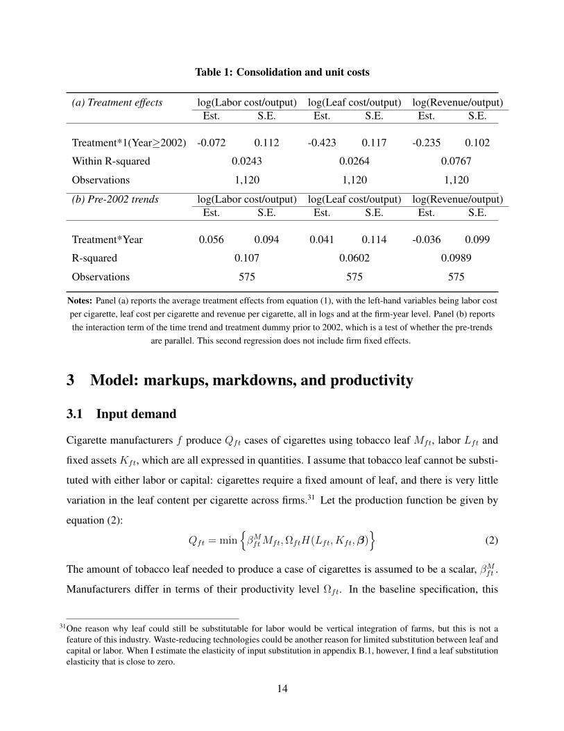
Table 1: Consolidation and unit costs

(a) Treatment effects log(Labor cost/output) log(Leaf cost/output) log(Revenue/output)Est. S.E. Est. S.E. Est. S.E.

Treatment*1(Year≥2002) -0.072 0.112 -0.423 0.117 -0.235 0.102

Within R-squared 0.0243 0.0264 0.0767

Observations 1,120 1,120 1,120

(b) Pre-2002 trends log(Labor cost/output) log(Leaf cost/output) log(Revenue/output)Est. S.E. Est. S.E. Est. S.E.

Treatment*Year 0.056 0.094 0.041 0.114 -0.036 0.099

R-squared 0.107 0.0602 0.0989

Observations 575 575 575

Notes: Panel (a) reports the average treatment effects from equation (1), with the left-hand variables being labor costper cigarette, leaf cost per cigarette and revenue per cigarette, all in logs and at the firm-year level. Panel (b) reportsthe interaction term of the time trend and treatment dummy prior to 2002, which is a test of whether the pre-trends

are parallel. This second regression does not include firm fixed effects.

3 Model: markups, markdowns, and productivity

3.1 Input demand

Cigarette manufacturers f produce Qft cases of cigarettes using tobacco leaf Mft, labor Lft and

fixed assets Kft, which are all expressed in quantities. I assume that tobacco leaf cannot be substi-

tuted with either labor or capital: cigarettes require a fixed amount of leaf, and there is very little

variation in the leaf content per cigarette across firms.31 Let the production function be given by

equation (2):

Qft = minβMftMft,ΩftH(Lft, Kft,β)

(2)

The amount of tobacco leaf needed to produce a case of cigarettes is assumed to be a scalar, βMft .

Manufacturers differ in terms of their productivity level Ωft. In the baseline specification, this

31One reason why leaf could still be substitutable for labor would be vertical integration of farms, but this is not afeature of this industry. Waste-reducing technologies could be another reason for limited substitution between leaf andcapital or labor. When I estimate the elasticity of input substitution in appendix B.1, however, I find a leaf substitutionelasticity that is close to zero.

14

productivity term is assumed to be a scalar, but this can be generalized.32 Firms use a production

technology H(.) in labor and capital with common parametrization β. I assume H(.) is twice

differentiable in both labor and capital. In the baseline model, there is no measurement error in

output.33 Equation (2) nests production functions in which all inputs are substitutable: the input

requirement βMft would then be zero, and leaf would be an additional subtitutable input in H(.).

I assume that manufacturers produce a single product, cigarettes, at a price Pft.34 Cigarettes are

vertically differentiated across firms, with an unobserved, firm-level quality index ζft. This quality

level is assumed to be exogenous to the manufacturers. In section 4.1, I discuss more in detail how

endogenous quality choices would affect identification of the model. I remain agnostic about the

cigarette demand function faced by the manufacturers and about competition downstream.

Assumption 1. — Cigarette quality ζft is exogenous from the point of view of each individual

manufacturer f .

Input markets Leaf is sold at a monthly frequency without the use of forward contracts. I

therefore assume that tobacco leaf is a variable input: it is chosen in the same time period as when

it is used. I also assume that tobacco leaf is a static input, which means that it only affects current

profits. This rules out adjustment costs or inventories. Labor is assumed to be a variable and static

input as well. Cigarette manufacturing factories rely mainly on production workers, for which

these assumptions are more likely to hold compared to white-collar workers.35 This is not crucial

to the model, which can be easily extended to allow for violations of the static input assumption

due to hiring or firing costs. Capital is, in contrast, dynamic and fixed: the capital stock at time t

can only be changed at time t− 1 through investment I. It depreciates at a rate η > 0:

Kft = ηKft−1 + Ift−1

The prices of leaf and labor are WMft and WL

ft. The extent of oligopsony power of a manufac-

32I discuss evidence against important differences in factor-augmenting productivity in this industry in appendix B.2.33I extend the model to allow for measurement error in output in appendix D.2.34The model can be generalized to a multi-product setting using De Loecker et al. (2016), but this is not of first-order

importance for the tobacco industry as cigarettes make up for 90% of sales on average.35The NBS surveys does not distinguish production from non-production workers, but 70% of US cigarette manufactur-

ing employees and 65% of the wage bill were production workers, and hence variable, in 1997 (U.S. Census Bureau,1997)

15

turer f over an input V ∈ L,M is parametrized by the inverse input supply elasticity ψVft:

ψVft ≡∂W V

ft

∂Vft

VftW Vft

+ 1 ≥ 1

If a manufacturer has oligopsony power over input V , the input price W V increases if more inputs

are purchased, meaning that ψVft > 1. If the price of an input V is exogenous to a manufacturer,

this implies that ψVft = 1. I specify a full model of the input supply functions and input market

competition in section 3.3.

Manufacturer decisions Variable profits are defined as Πft ≡ PftQft − WMftMft − WL

ftLft.

The usual assumption in the ‘cost-side’ approach to markup identification is that firms choose

inputs to minimize their costs, given a certain level of output. Given that intermediate inputs are

non-substitutable, however, their level can only be changed by also changing output.36 I therefore

assume that firms choose the output level that maximizes their current variable profits:

maxQft

(PftQft −WM

ftMft −WLftLft

)(3)

Assumption 2. — Firms choose their output in each period in order to maximize their current

variable profits Πft.

The profit maximization assumption can be questioned: it is often suggested that state-owned

enterprises (SOEs) have non-profit objectives, such as generating local employment (Lu and Yu,

2015). In the tobacco industry, however, Peng (1996) notes that cigarette manufacturers have

“the purpose of making profits” and “often bargain with each other for better deals”.37 Next, leaf

prices were in theory regulated by the government. In reality, however, manufacturing firms had

considerable pricing power on leaf markets from the 1980s onwards. Conflicts between peasants

and manufacturers over leaf prices are frequent, and farmers show up at a purchasing point without

knowing leaf prices on beforehand Peng (1996).38 Next, the assumption that firms can change their

input prices by choosing their output levels can be questioned as well, as leaf prices are officially

regulated. Manufacturing firms bypass these regulations, however, by gaming quality grades and

36This also implies that changes in oligopsony power affects the optimal output level, which I verify in section 4.3.37In appendix B.5, I extend the model to allow for objective functions other than profit maximization.38More details on leaf pricing strategies in the Chinese setting are in appendix B.6.

16

by controlling local STMA boards. I refer to appendix B.6 for a more detailed discussion of these

institutional features.

3.2 Markups and markdowns

The profit maximization problem implies the following first order condition, which has marginal

revenue on the left hand side and marginal costs λft on the right.

∂(PftQft)

∂Qft︸ ︷︷ ︸Marginal revenue

=∂(WM

ftMft +WLftLft)

∂Qft︸ ︷︷ ︸Marginal cost

≡ λft

Marginal costs do not depend only on input prices and output elaticities of inputs, but also on the

slope of the input supply curves ψVft. The reason for this is that increasing output endogenously

increases input prices as well if the input supply curves are upward-sloping:

λft = WLftψ

Lft

∂Lft∂Qft

+WMft ψ

Mft

∂Mft

∂Qft

Markups The markup ratio µ is the ratio of factory-gate prices over marginal costs: µft ≡ Pftλft

.

Substituting the marginal cost expression into the markup formula results in equation (4a), with

the revenue shares of each input being denoted as αVft ≡VftW

Vft

PftQft

, with V ∈ L,M.

µft =(αLftβLft

ψLft + αMftψMft

)−1

(4a)

This markup expression looks different compared to the typical markup expression from De Loecker

and Warzynski (2012), in which it is the ratio of an output elasticity over a revenue share, for two

reasons. First, equation (4a) has an additive structure, because of the complementarity of labor

and intermediate inputs. Each variable input cannot be changed without changing the other input

as well. Second, the markup expression contains the input price elasticities ψLft and ψMft because

these enter the marginal cost curve, as was explained before.

Special cases The markup expression in equation (4a) nests previous markup models. I discuss

three special cases that were used in the prior literature. First, suppose all inputs have exogenous

prices and are mutually substitutable. In that case, the non-substitutable input revenue share is

17

by definition zero, αMft = 0, and the input supply functions are flat: ψVft = 1 , ∀V . The markup

expression then simplifies to the formula of De Loecker and Warzynski (2012):

µft =βLftαLft

(4b)

Next, consider a setting in which all inputs are substitutable, but in which input prices are

endogenous. The markup is now expressed as the output elasticity of a variable input divided by

its revenue share and divided by its inverse supply elasticity. This corresponds to the expression

from Morlacco (2017).

µft =βLft

αLftψLft

(4c)

Finally, assume that all input prices are exogenous, but that there is a non-substitutable input

M : αMft > 0 but (ψVft) = 1, ∀V . The markup is given by equation (4c), which corresponds to

expression from De Loecker and Scott (2016).

µft =(αLftβLft

+ αMft

)−1

(4d)

Markdowns The inverse supply elasticity ψVft has the interpretation of an input price ‘markdown

ratio’. Re-arranging marginal costs in function of the input price elasticity of leaf ψMft gives the

following expression:

ψMft =

M.P.︷︸︸︷λft −

(M.C. of labor︷ ︸︸ ︷WLftψ

Lft

∂Lft∂Qft

)WMftMft

Qft︸ ︷︷ ︸Leaf cost per cigarette

The parameter ψMft hence indicates the extent to which the marginal benefit of tobacco leaf to

the manufacturer, which is the marginal product of cigarettes minus the marginal cost of labor,

exceeds the leaf cost per cigarette. If ψMft = 2, this implies that tobacco farmers receive 50% of

their marginal benefit to the cigarette manufacturer. In the literature, the markdown is often also

defined as a ‘markdown wedge’ δMft , which is the extent to which the leaf price is marked down

18

below its marginal benefit. This wedge is the following function of the markdown ratio:

δMft ≡λft −WL

ftψLft∂Lft∂Qft− WM

ftMft

Qft

λft −WLftψ

Lft∂Lft∂Qft

=ψMft − 1

ψMft

For the purpose of clarity, I will only report and discuss the markdown ratio ψMft , and refer to this

ratio as ‘the markdown’. The markdown ratio has the advantage of being scaled similarly to the

markup ratio µ, with a support on [0,∞] and a value of one that corresponds to exogenous prices.

Moreover, the product of ψMft and µft has the interpretation of a variable profit margin. This means

that firms can operate at a positive variable profit even if the markup is below one: there is a wedge

both between the product price and marginal costs, and between marginal costs and input prices.

Identification In the typical production-cost dataset, the revenue shares αMft and αLft are ob-

served. If all input prices are exogenous, identification of the production function suffices to iden-

tify the markup, as can be seen in equations (4b) and (4d). If input prices are endogenous, both

markups and markdowns can still be identified by only identifying the production function if all

inputs are substitutable, and if there is at least one variable input of which the price is exogenous.

This can be seen from equation (4c): markdowns can be found by dividing each markup that is

obtained using an input with an endogenous price by the markup that is expressed using the input

with the exogenous price. In the general case with both non-substitutable inputs and endogenous

input prices of equation (4a), however, the unknown parameters are the markup µft, the mark-

downs ψMft and ψLft, and the output elasticity of labor βLft. Only knowing βLft is insufficient to

identify the markup: the wedge between the output elasticity of an input and its revenue share can

be due to both market power upstream or downstream.

There are three potential identification strategies to still identify markups from markdowns.

A first possibility is to identify the markdowns ψLft and ψMft by applying the ‘demand approach’

from empirical industrial organization to the input supply side. The input supply elasticities ψMft

and ψLft can be identified using input price and quantity data, a functional form assumption on

the input supply functions, and a model of how manufacturers compete on their input markets.

In combination with the output elasticity βLft, which can be identified following the production

function literature, this leads to identification of the markup µft without having to impose a model

of demand for cigarettes and of how manufacturers compete downstream. A second possibility

19

is to impose a model of how firms compete on the wholesale market and on cigarette demand,

in order to identify the markup µft. If the production function is identified as well, it is possible

to recover the input supply elasticity of at most one input without taking a stance on the supply

function of, and competition for, that input. This approach requires observing wholesale cigarette

prices and product characteristics, and ideally also retail prices. Finally, one could also combine

supply models for each input with a demand model for cigarettes, and remain agnostic about the

production function.

The optimal identification strategy depends both on which data are available, and on the nature

of competition on input and product markets. In the context of tobacco manufacturing, I choose to

combine an input supply model with a production model and to remain agnostic about cigarette de-

mand and competition downstream. Leaf supply is easier to model than cigarette demand because

the latter is inherently dynamic due to addiction. Moreover, the vertical structure of the cigarette

market, with wholesalers and retailers, is harder to model than leaf and labor markets, where there

are no independent intermediaries. Cigarette markets are, finally, geographically not as delineated

as leaf markets.

3.3 Input supply

In this section, I impose a model of input supply and of how manufacturers compete on their input

markets, in order to identify the markdowns ψLft and ψMft . The labor and capital supply models

are simple: I assume that manufacturing worker wages are exogenous to manufacturers and that

capital markets are perfectly competitive, which means that ψLft = 1. These assumptions are not

strictly necessary, but I impose them because labor wages did not adjust much in response to the

consolidation, and both the markets for manufacturing workers and capital do not share the leaf

markets’ institutional feature of being geographically isolated due to transportation restrictions.

For leaf supply, I rely on a discrete choice model with differentiated firms in the tradition

of Berry (1994).39 Farmers j sell tobacco leaf on an isolated market i in year t to at most one

manufacturing firm f ∈ Fit, with f = 0 indicating the outside option of not selling to any firm.

I assume each firm operates in exactly one market and that farmers sell their entire production

to a single firm, which makes sense as there were 8 million tobacco farms but merely 350 firms

39Azar et al. (2019) is a contemporaneous paper which also applies Berry (1994) to the context of input markets, butwith a focus on employees and using a different type of data.

20

in 1999 (FAO, 2003). A farmer j derives a utility from selling to firm f , which depends on the

leaf price WMft , observed firm characteristics Xft, latent characteristics ξft, cigarette quality ζft,

and a firm-farmer specific utility term νjft. Examples of manufacturer characteristics that enter

farmer utility could be state ownership, which is observed, or the distance between the factory

and a major highway, which is latent. An example of the farmer-manufacturer specific utility

shock νjft could be accidental encounters between farmers and manufacturing employees that

facilitate trading relationships. The utility derived from the outside option is normalized to zero.

The cigarette quality scalar ζft enters farmer utility as higher quality leaves are costlier to grow.

High-quality leaf is required to produce high-quality, high-price cigarettes. Quality levels were

assumed to be exogenous in assumption 1.

Ujft = γWWMft + γXXft + ξft + ζft + νjft

I assume that farmers periodically choose which manufacturer to sell to by maximizing their static

utility. They may not choose the manufacturer that offers the highest price because of the non-

price characteristics that enter the utility function. In the baseline model, I assume that there is

no heterogeneity in the coefficients γW and γX : all farmers hold the same preferences over leaf

prices and manufacturer characteristics. I also assume that the farmer-firm specific utility term νjft

follows an i.i.d. type-I distribution, which means that if firm f is particularly attractive to a certain

farmer today, but not to other farmers, this does not contain information about its attractiveness to

this same farmer in the future. Both these assumptions are reasonable in the context of Chinese

tobacco because there is not much of a relationship between the farmers and the manufacturers

other than transacting money: it is hence likely that farmers mainly care about the leaf price they

get and about the cost of transporting leaf to the firm. Farmer choices are assumed to be static. The

elasticities that are recovered are, hence, short-run elasticities.

Assumption 3. — The farmer-manufacturer utility shock νjft follows an extreme-value type-I

distribution.

Competition on leaf markets I follow the usual differentiated Bertrand model, which assumes

that manufacturing firms simultaneously choose tobacco leaf prices each period in order to max-

imize their profits. This seems contradictory to the production model, which assumed that firms

21

choose their profit-maximizing output levels. Leaf prices are, however, a function of leaf quantities

through the leaf supply function, and cigarette and leaf quantities are proportional due to the non-

substitutability of leaf. The assumption in the production model that firms simultaneously choose

output levels is hence equivalent to the assumption that they simultaneously choose leaf prices.40

The leaf market share of firm f in year t is denoted as Sft =Mfjt∑

r∈FitMfrt

. Assuming that a pure

strategy interior equilibrium exists, and making use of the distributional assumption about νjft, the

first order condition for every firm can be rewritten as follows (Berry, 1994):

Sft =exp(γWWM

ft + γXXft + ξft + ζft)∑r∈Fit exp(γWWM

rt + γXXrt + ξrt + ζrt)

Dividing this share by the market share of the outside option S0t, of which the utility is nor-

malized to zero, and taking logarithms leads to equation (5), which can be estimated.

sft − s0t = γWWMft + γXXft + ξft + ζft (5)

The leaf price markdown ψMft is a function of input prices, input market shares, and the price

valuation coefficient γW :

ψMft ≡( ∂Sft∂WM

ft

WMft

Sft

)−1

+ 1 =(γWWM

ft (1− Sft))−1

+ 1 (6)

I choose to impose the strong assumptions about substitution elasticities and functional forms in

the leaf supply model because the former can be defended in the context of this industry, and

because the data set is of a small size. These assumptions can, however, be relaxed.41

4 Empirical analysis

4.1 Production function

Taking the logarithm of the production function, equation (2), results in equation (7a). As tobacco

leaf is assumed to be non-substitutable and a linear function of the number of cigarettes, it does

40I show this in appendix D.1.41One could, for instance, allow for random coefficients, as in Berry et al. (1995).

22

not enter the estimable production function.42 The production coefficients β need to be identified.

qft = h(lft, kft,β) + ωft (7a)

Product differentiation Cigarettes are differentiated products, with important quality differ-

ences. Output is observed in physical units, which solves the ‘output price bias’ described in

De Loecker et al. (2016). Labor inputs are observed in units as well, but potentially with error:

rather than observing the total hours worked lft, I observe the number of employees lft. Capital

is measured in monetary values kft, rather than in physical units kft, so any variation in capital

prices due to differences in technological sophistication are latent as well. If these latent hours

worked and input quality differences are correlated with cigarette quality, this induces an ‘input

price bias’ (De Loecker et al., 2016). This is likely to be the case for the tobacco industry. The

luxury cigarette segments, which are mainly used as gifts, have features which take more labor

hours, such as handcrafted packs. I follow De Loecker et al. (2016) by adding a function a(.) of

wages per worker and cigarette prices to the production function to address this input price bias.43

Although tobacco leaf is differentiated in terms of quality levels as well, this does not induce input

price bias because leaf does not enter the estimable production function.

qft = h(lft, kft,β) + a(pft, wLf,t) + ωft (7b)

Identification In order to identify the production function, I impose timing assumptions on

firms’ input choices, as proposed by Olley and Pakes (1996). Let the productivity transition be

given by the AR(1) process in equation (8b), with an unexpected productivity shock υft.44

ωft = g(ωft−1) + υft (8a)

42The usual caveat applies that it could be optimal for firms to diverge from equation (7a) by setting intermediate inputsto zero if material prices become too high, or output prices too low (Gandhi et al., 2020). Given that intermediateinputs enter the production function linearly, however, this would imply that firms do not produce at all, at which pointthey no longer enter the dataset.

43I refer to De Loecker et al. (2016) for a formal model and discussion of input price bias.44One could object that this equation of motion already rules out that the consolidation affected total factor productivity,

as was its official goal (Braguinsky et al., 2015; De Loecker, 2013). As an extension, I specify a law of motion forproductivity that allows for such endogeneity of productivity in appendix C.2, with very similar results.

23

In section 3.1, it was assumed that labor is a variable and static input, while capital is fixed

and dynamic. Labor is hence assumed to be chosen at time t, after the productivity shock υft is

observed by the firm, while capital investment is chosen at time t−1, before the productivity shock

is observed. Cigarette and worker quality, which are proxied by cigarette prices and wages, were

already assumed to be strictly exogenous from the point of view of the manufacturers. These timing

assumptions lead to the following exclusion restrictions: the productivity shock is orthogonal to

current capital usage, coal prices and wages, and to lagged labor usage.45

E[υft|(lfr−1, kfr, pfr, w

Lfr)]r∈[2,...,t]

= 0

The usual approach in the literature is to invert the intermediate input demand function to recover

the latent productivity level ωft, which can be used to construct the productivity shock υft using the

productivity law of motion (Levinsohn and Petrin, 2003; Ackerberg et al., 2015). This approach

hinges on productivity being the only latent serially correlated input demand shifter. Input demand

varies, however, due to markup and markdown variation as well. The approach with input inversion

can still be used when making additional parametric assumptions about the distribution of markups

and markdowns.46 Another possibility is to impose more structure on the productivity transition

process. Following Blundell and Bond (2000), the productivity transition can be rewritten as a

linear function with serial correlation ρ, equation (8b). By taking ρ differences of equation (8b),

one can express the productivity shock υft as a function of estimable coefficients without having

to invert the input demand function.

ωft = ρωft−1 + υft (8b)

The key benefit of this linearization is that it does not impose any structure on the distribution of

markups and markdowns across firms and over time. This comes at the cost of ruling out a richer

productivity transition function g(.), and of not coping with selection bias due to endogenous en-

try and exit. As is often noted in the literature, however, moving to an unbalanced panel already

45In theory, one could also add the future values for P and WL as instruments, but this would come at the cost ofreducing the size of the data set.

46I refer to appendix C for a discussion.

24

alleviates most concerns of selection bias.47 Exit in the industry was, moreover, mainly the result

of being subject to the consolidation treatment, which is assumed to be exogenous to the manufac-

turers anyway. Considering that this paper seeks to answer how markups and markdowns evolve

over time across different groups of firms, the dynamic panel approach hence seems to have the

more attractive set of assumptions, which is why I use it as the baseline identification strategy. In

appendix C, I discuss how the results change when using the control function approach with input

inversion of Ackerberg et al. (2015).

Estimation In the baseline specification, I use a Cobb-Douglas specification for both the h(.) and

a(.) functions: h(lft, kft) = βLlft + βK(kft) + β0 and a(wLft, pft) = βWwLft + βPpft.48 Rewriting

the moment conditions above, and only using the lags up to one year, the moment conditions are

given by equation (9).49

E[(qft − ρqft−1)− β0(1− ρ)− βK(kft − ρ(kft−1))− βL(lft − ρlft−1)

− βW (wLft − ρwLft−1)− βP (pft − ρpft−1)|(lf−1, kft, kft−1, wLft, w

Lft−1, pft, pft−1)

]= 0 (9)

4.2 Input supply function

Identification Next, I turn to the identification of the input supply function, equation (5). Leaf

pricesWMft and quantitiesMft are not observed separately in the data, as usual. I impose, however,

that manufacturers do not differ in terms of leaf content, βMft = βM .50 This allows recovering the

leaf price up to a constant by dividing leaf expenditure by the number of cigarettes produced:

WMft =

WMftMft

QftβM .

As the manufacturers know that the latent manufacturer characteristics ξft affect the utility

of the suppliers, they take this into account when setting their leaf prices. In order to separately

identify input demand and supply, an input demand shifter can be used as an instrument for input

prices. I rely on manufacturing productivity ωft, which was estimated in the previous section, as an

instrumental variable. As productivity enters the input demand function, it is by definition relevant.

47Cfr. Olley and Pakes (1996), De Loecker et al. (2016).48In appendix B.3, I estimate a translog production function instead.49In theory, one could use more lags, but this further reduces the data set, which is already small.50Additional brand-level data reveal very little variation in leaf contents per cigarette across manufacturers. I discuss the

consequences of leaf content heterogeneity in appendix B.4.

25

The exclusion restriction is that the productivity term does not enter the supplier utility function,

meaning that it is orthogonal to the supply function residual ξft + ζft, which includes both latent

manufacturer ‘attractiveness’ ξft and cigarette quality ζft.51

E[(ξft + ζft)(ωft,Xft)] = 0

The moment condition above implies two key assumptions about leaf supply. First, farmers

do not care how efficient the manufacturing firms are which they are selling to, conditional on the

leaf price and on observable manufacturer characteristics. Productivity differences between manu-

facturers can have many reasons, such as differences in managerial ability. As the farmers are not

employed by the manufacturers, but only interact with these firms through monetary transactions

on leaf markets, it seems reasonable that the farmers do not care about how productive their buyers

are conditional on the price they receive. One threat to the validity of this assumption could be

that suppliers prefer to sell repeatedly to the same buyers. This is the case in many industries that

are characterized by incomplete contracts or weak contract enforceability.52 Search or switching

costs on the seller side could be another driver of why repeated interaction would be valuable.53

In all these cases, sellers would prefer a more productive buyer as it is less likely to exit in the

future, even if offering a lower price. In the Chinese tobacco industry, however, this is not likely

to be a major concern because leaf markets do not make use of long-term contracts. Moreover,

as was mentioned before, exit is mainly driven by government policies, which are assumed to be

exogenous to individual manufacturers, rather than by productivity differences.

A second assumption that follows from the moment condition is that conditional on cigarette

prices, cigarette quality is independent from total factor productivity. As was mentioned earlier,

higher-quality cigarettes could require more labor and capital inputs, which would be reflected in

a lower physical productivity level. Cigarette prices are, however, included in the utility function,

and were already assumed to proxy for cigarette quality when identifying the production function.

51Productivity is by definition uncorrelated with the farmer-utility specific utility term νjft, which was already assumedto be i.i.d. across manufacturers and over time.

52The literature on vertical relationships in developing countries has emphasized the importance of relational contractsand repeated interaction (Macchiavello and Morjaria, 2015).

53When applying the same model for manufacturing labor markets, more caution is needed. There are many reasons whyemployees would prefer to work for highly productive firms, even if these offer lower wages, such as career dynamicsor better working conditions.

26

The identification challenge from differentiated products is hence the same for the production

function and the leaf supply function, and if the price control solves this problem for the production

function, it should do so for the leaf supply function as well. Moreover, using the brand-level data

on product characteristics reveals that the physical productivity of cigarette manufacturers does not

correlate significantly with any product characteristic or quality indicator.54 Finally, the variation

in leaf cost shares could be due to endogenous quality choices, which were abstracted from in the

model. If this were true, there would be both a leaf price markdown and a quality markdown. In

order to reconcile falling leaf cost shares, though, quality would have had to drop sharply over the

time period studied, whereas consumer surveys report that Chinese cigarette quality improved over

time (Hu, 2008).

Estimation I estimate equation (5) using 2SLS with the manufacturing productivity residual Ωft

as an instrument for the leaf price. In order to calculate the leaf market share, the outside option

needs to be defined: how many tobacco farmers could have been farming tobacco, but chose not

to do so? As there is barely any crop switching towards or from tobacco leaf (Li et al., 2012), I

model the outside option of tobacco farming as being employed in non-agricultural occupations. I

therefore set the outside option market share equal to the share of the population that works in non-

agricultural sectors, which is observed from the population census. The problem is, however, that

I do not have this data for all prefectures in the data set, which reduces the number of observations

to 956. In order to keep the full data set, I therefore set leaf markets at the province-level for

the estimation of the leaf supply function, at which level the outside option has a market share of

36.7% on average. In appendix B.7, I use both prefecture- and province-level market definitions

to estimate the markdown, with very similar conclusions about the effects of the consolidation.

I include three manufacturer characteristics in the vector of supply shifters Xft. First, I control

for cigarette prices, as they are a proxy for quality. Second, I control for manufacturer ownership

types, in order to proxy political pressure: farmers may derive a different utility from selling to

manufacturers that are state-owned rather than private. Finally, I include prefecture dummies to

control for the geographical differences.

In order to estimate the leaf supply function, the productivity residuals from the production

function are needed. I therefore estimate the production function and leaf supply function sequen-

54This evidence is shown in appendix table A5(b).

27

tially, and bootstrap the entire estimation procedure. I use a block bootstrap that resamples entire

firm time series with 50 iterations.

4.3 Results

The estimated output elasticities are in table 2(a). The estimates using the dynamic panel approach

are in the right column, and are 0.591 and 0.592 for labor and capital. These estimates are respec-

tively lower and higher compared to the OLS estimates, as usual.55 Both specifications have a scale

parameter that is significantly above one, which implies increasing returns to scale.

The estimates of the leaf supply function, equation (5), are in table 2(b). The OLS estimate

for the leaf price coefficient in the supply curve, γW , is negative, but does not take into account

that leaf prices are endogenous to latent manufacturer characteristics. When using the instrumental

variables approach, the leaf price coefficient becomes 0.547. The standard error is large, but does

not imply that the leaf price coefficient is insignificant. The bootstrapped standard errors show

that the leaf price coefficient lies above 0.15 with a probability of 95%.56 The leaf supply curve

is hence upward-sloping. In order to interpret its magnitude, it has to be transformed into a leaf

supply elasticity, which I do below. The first stage regression has an F-statistic of 188, so the

instrument is strong.

Markups and markdowns I calculate the leaf price markdown using equation (6) and the esti-

mated leaf supply coefficients. Combined with the output elasticity of labor βL, which is estimated,

and the revenue shares αLft and αMft , which are observed, markups can be inferred using equation

(4a). I include the markdown and markup estimation in the block bootstrapping procedure. Se-

lected moments of the markup and markdown distributions are in table 3.57 The average markdown

ratio is 5.307 , which implies that farmers who sell leaf to the average manufacturer receive around

a fifth of what they would receive in the absence of oligopsony power. The 90% confidence inter-

val lies between 1.239 and 11.864, so markdowns are significantly above one at the 5% level. The

average firm therefore has oligopsony power on the tobacco leaf market. The median manufacturer

has a leaf price markdown ratio of 4.379, which means that farmers who sell to this median firm

55In appendix C.1, I estimate the model using the control function approach with input demand inversion of Ackerberget al. (2015).

56The difference between the confidence interval and the standard error may be due to non-normally distributed leafsupply residuals.

57Both distributions are winsorized at the 1th and 99th percentiles.

28

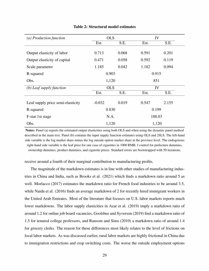
Table 2: Structural model estimates

(a) Production function OLS IVEst. S.E. Est. S.E.

Output elasticity of labor 0.713 0.068 0.591 0.201

Output elasticity of capital 0.471 0.058 0.592 0.119

Scale parameter 1.185 0.042 1.182 0.094

R-squared 0.903 0.915

Obs. 1,120 851

(b) Leaf supply function OLS IVEst. S.E. Est. S.E.

Leaf supply price semi-elasticity -0.032 0.019 0.547 2.155

R-squared 0.830 0.199

F-stat 1st stage N.A. 188.03

Obs. 1,120 1,120

Notes: Panel (a) reports the estimated output elasticities using both OLS and when using the dynamic panel methoddescribed in the main text. Panel (b) contains the input supply function estimates using OLS and 2SLS. The left-handside variable is the log market share minus the log outside option market share at the province level. The endogenous

right-hand side variable is the leaf price for one case of cigarettes in 1000 RMB. I control for prefecture dummies,ownership dummies, product dummies, and cigarette prices. Standard errors are bootstrapped with 50 iterations.

receive around a fourth of their marginal contribution to manufacturing profits.

The magnitude of the markdown estimates is in line with other studies of manufacturing indus-

tries in China and India, such as Brooks et al. (2021) which finds a markdown ratio around 5 as

well. Morlacco (2017) estimates the markdown ratio for French food industries to be around 3.5,

while Naidu et al. (2016) finds an average markdown of 2 for recently hired immigrant workers in

the United Arab Emirates. Most of the literature that focuses on U.S. labor markets reports much

lower markdowns. The labor supply elasticities in Azar et al. (2019) imply a markdown ratio of

around 1.2 for online job board vacancies, Goolsbee and Syverson (2019) find a markdown ratio of

1.5 for tenured college professors, and Ransom and Sims (2010) a markdown ratio of around 1.4

for grocery clerks. The reason for these differences most likely relates to the level of frictions on

local labor markets. As was discussed earlier, rural labor markets are highly frictional in China due

to immigration restrictions and crop switching costs. The worse the outside employment options

29

of farmers, the higher markdowns should be. I refer to appendix D.7 for correlations between the

markdown estimates and firm and market characteristics.

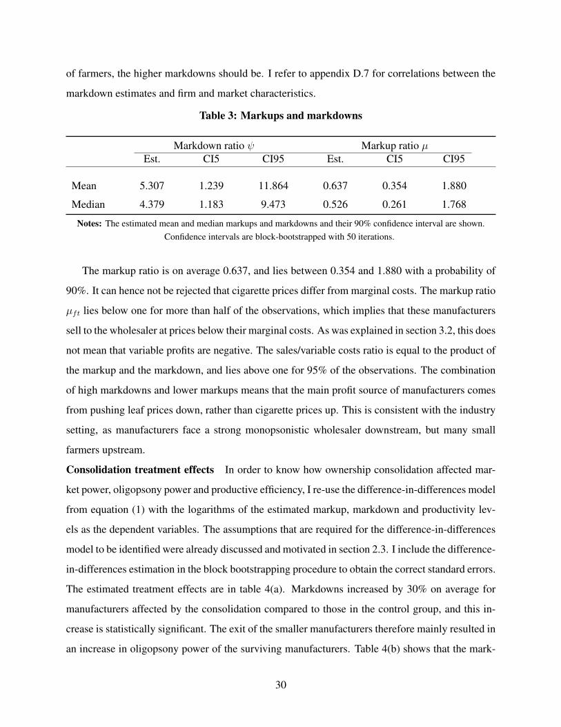
Table 3: Markups and markdowns

Markdown ratio ψ Markup ratio µEst. CI5 CI95 Est. CI5 CI95

Mean 5.307 1.239 11.864 0.637 0.354 1.880

Median 4.379 1.183 9.473 0.526 0.261 1.768

Notes: The estimated mean and median markups and markdowns and their 90% confidence interval are shown.Confidence intervals are block-bootstrapped with 50 iterations.

The markup ratio is on average 0.637, and lies between 0.354 and 1.880 with a probability of

90%. It can hence not be rejected that cigarette prices differ from marginal costs. The markup ratio

µft lies below one for more than half of the observations, which implies that these manufacturers

sell to the wholesaler at prices below their marginal costs. As was explained in section 3.2, this does

not mean that variable profits are negative. The sales/variable costs ratio is equal to the product of

the markup and the markdown, and lies above one for 95% of the observations. The combination

of high markdowns and lower markups means that the main profit source of manufacturers comes

from pushing leaf prices down, rather than cigarette prices up. This is consistent with the industry

setting, as manufacturers face a strong monopsonistic wholesaler downstream, but many small

farmers upstream.

Consolidation treatment effects In order to know how ownership consolidation affected mar-

ket power, oligopsony power and productive efficiency, I re-use the difference-in-differences model

from equation (1) with the logarithms of the estimated markup, markdown and productivity lev-

els as the dependent variables. The assumptions that are required for the difference-in-differences

model to be identified were already discussed and motivated in section 2.3. I include the difference-

in-differences estimation in the block bootstrapping procedure to obtain the correct standard errors.

The estimated treatment effects are in table 4(a). Markdowns increased by 30% on average for

manufacturers affected by the consolidation compared to those in the control group, and this in-

crease is statistically significant. The exit of the smaller manufacturers therefore mainly resulted in

an increase in oligopsony power of the surviving manufacturers. Table 4(b) shows that the mark-

30

down trend was not significantly different between the control and treatment group prior to 2002.

Although markdown levels were higher for the firms in the control group, this difference was en-

tirely due to the larger size of firms in markets that were already concentrated prior to the start of

the policy. Controlling for size, markdowns were initially not significantly different between the

treatment and control group.58

Table 4: Consolidation treatment effects

(a) Treatment effects log(Markdown) log(Markup) log(Productivity)Est. S.E. Est. S.E. Est. S.E.

Treatment*1(Year≥ 2002) 0.259 0.121 -0.084 0.098 -0.066 0.082

R-squared 0.804 0.775 0.848

Obs. 1,120 1,120 1,120

(b) Pre-2002 trends log(Markdown) log(Markup) log(Productivity)Est. S.E. Est. S.E. Est. S.E.

Treatment*Year if Year< 2002 -0.010 0.043 -0.070 0.059 -0.165 0.066

R-squared 0.105 0.0156 0.133

Obs. 581 581 581

Notes: Panel (a) reports the estimated treatment effects from equation (1) with the logarithms of the markdown ratio,markup ratio and productivity as the dependent variable. Controls include firm and year fixed effects. Panel (b)estimates the pre-trends in the three dependent variables prior to the intervention in 2002. Standard errors are

block-bootstrapped with 50 iterations.

In contrast to markdowns, cigarette markups fell by 8% for firms in consolidated markets com-

pared to the control group, although this drop was not statistically significant. The results in panels

4(b)-(c) show that markups were similar and moved in parallel between both groups before 2002.

Imposing prefecture-level markets may, however, be a source of misspecification for the estimated

markup changes, as cigarette markets are not limited to the prefecture level. I therefore re-estimate

the difference-in-differences model at the province-level in table A6(a). When using this wider

market definition, manufacturing markups fell by 18% due to the consolidation, and this change is

significantly below zero.

58Pre-intervention markdown, markup and productivity levels are compared in table A11(a)-(b), both when controllingfor size and when not.

31

The fact that factory-gate price markups fall in response to increasing concentration is, at first

sight, less intuitive than the rise of leaf price markdowns. One has to keep in mind, however, that

the wholesaler, which is a monopsonist, is likely to have buyer power over factory-gate cigarette

prices, both before and after the consolidation. As manufacturing profits increased due to the drop

in leaf prices after the consolidation, it is natural that the wholesaler used its own bargaining power

to push down cigarette prices, and hence appropriate a part of the increased industry profits. In

appendix D.6, I formalize this argument using a simple bargaining model with double marginal-

ization.

Average productivity growth after 2002 was not significantly different between the treatment

and control group. Some caution is necessary when interpreting this result, though, as the pre-

trends in productivity are not parallel: productivity growth was significantly lower for firms in the

treatment group prior to the reform. This is not entirely surprising given that the central motivation

for the consolidation was to address lackluster productivity growth among the smaller producers.

Finally, the fact that the consolidation did not seem to increase productivity within firms over time

on average is not informative about the effects of the consolidation on aggregate productivity,

which I examine in the next section.

5 Aggregate consequencesI end the paper by discussing the aggregate consequences of the ownership consolidation at the

industry level. I focus both on its effects on the distribution of income, in section 5.1, and on

economic growth, in section 5.2.

5.1 Distributional consequences

The urban-rural income gap has risen sharply in China over the past two decades (Yang, 1999;

Ravallion and Chen, 2009). The tobacco industry, in which factory workers live mainly in urban

areas and tobacco farmers in rural areas, was no exception to this trend. While the average wage

of factory workers grew on average by 14.5% per year between 1999 and 2006, tobacco leaf prices

fell by 11%. In this section, I quantify the extent to which the consolidation of the cigarette

manufacturers contributed to this margin of inequality by increasing oligopsony power on leaf

markets, but not on manufacturing labor markets. The difference-in-differences model assumes

that leaf prices would have evolved similarly for firms in the control group and treatment groups

32

from 2002 onwards in the absence of the consolidation. I rewrite the difference-in-differences

equation (1) to have interaction terms between the treatment dummy and all time dummies:

log(WMft ) =

2006∑n=2000

(θ1nI(t = n) + θ2

nI(t = n)Zft

)+ θ3Zft + θ4 + υMft

The predicted leaf price in year t is WM,1ft = exp(θ1

t + θ2t + θ3 + θ4) for firms in the treatment group,

and WM,0ft = exp(θ1

t + θ4) for firms in the control group. The counterfactual leaf prices without

consolidation are denoted as WM,1ft and WM,0

ft for firms in the treatment and control group. For

firms in the treatment group, the leaf price would follow the evolution of leaf prices in the control

group from 2002 onwards. For firms in the control group, nothing would change: WM,0ft = WM,0

ftWM,1ft = exp(θ1

t + θ3 + θ4) if t ≥ 2002

WM,1ft = WM,1

ft if t < 2002

Results I calculate the average predicted leaf price per year both in reality and in the counterfac-

tual without consolidation by weighting the predicted prices for the treatment and control groups

by the number of firms in each group. In figure 4, I plot the ratio of the average leaf price over

the average wage in reality (the solid line) and in the counterfactual world without consolidation

(the dashed line). Both series are normalized at 1 in 2001. In reality, wages quadrupled relatively

to leaf prices between 2001 and 2006. In the absence of the consolidation, however, wages would

have merely doubled compared to leaf prices. Manufacturing wages outgrew farmer wages at a

fast pace outside the tobacco industry as well, as manufacturing productivity growth skyrocketed

during the 2000s. These results suggest, however, that increased market power due to the consol-

idation contributed to an important extent to the increased widening between manufacturing and

farmer wages in the tobacco industry.

Caveats The analysis above is a partial equilibrium exercise, and hence comes with a number

of caveats. First, it ignores entry and exit of farmers: higher entry and/or lower exit of farmers in

response to higher leaf prices could have suppressed the rise in leaf prices in the absence of the

consolidation. Second, tobacco represents a large share of economic activity in some prefectures,

so changing leaf prices are likely to have affected equilibrium prices and wages in other sectors as

33

Figure 4: Consolidation and income inequality

01

23

4W

age/

Leaf

pric

e (2

001=

1)

1998 2000 2002 2004 2006Year

Wage/Leaf price, reality Wage/Leaf price, counterfactual

Notes: The solid lines plot change in average manufacturing wages and leaf prices compared to2002 (normalization: 2002=0). The dashed line plots the counterfactual leaf price evolution inthe counterfactual scenario in which the exit thresholds were not enforced.

well. Finally, besides tobacco leaf prices, farm productivity and agricultural input costs matter as

well for farm profits. Aggregate producer statistics from the Food and Agriculture Organization

(FAO) show, however, that farm sizes remained constant and yields per acre grew by merely 1.8%

per year during this time period, which was not enough to compensate falling leaf prices.59

5.2 Output and productivity growth

The effects of the consolidation on average manufacturer productivity could be very different

from its effects on aggregate productivity . Similarly to other types of market power, oligop-

sony power leads to deadweight losses and allocative inefficiency, and hence to lower aggre-

gate productivity and output.60 I test this using the decomposition of Olley and Pakes (1996).

Prefecture-level aggregate productivity is denoted Ωit, and is weighted by the number of workers:

Ωit ≡∑

f∈Fit

(ΩftLft∑f∈Fit

(Lft)

). Average prefectural productivity is denoted as Ωit. I estimate how

both aggregate and average productivity were affected by the consolidation by estimating equation

(1) at the prefecture level. As shown in table 5(a), the average productivity level did not change

due to the consolidation, whereas aggregate productivity fell by 23%.

Under the assumptions of the classical oligopsony model used in this paper, higher oligopsony

power should lead to lower equilibrium amounts of cigarettes produced. This is a testable implica-

59Source: FAO statistical database, accessed through http://www.fao.org/faostat/en/ on October 2, 2019.60See (Asker et al., 2019; Edmond et al., 2018) for evidence on the effects of oligopoly power on allocative efficiency.

34

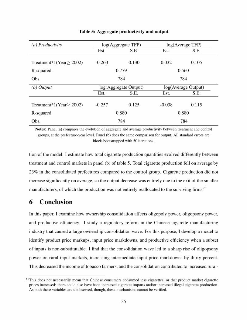
Table 5: Aggregate productivity and output

(a) Productivity log(Aggregate TFP) log(Average TFP)Est. S.E. Est. S.E.

Treatment*1(Year≥ 2002) -0.260 0.130 0.032 0.105

R-squared 0.779 0.560

Obs. 784 784

(b) Output log(Aggregate Output) log(Average Output)Est. S.E. Est. S.E.

Treatment*1(Year≥ 2002) -0.257 0.125 -0.038 0.115

R-squared 0.880 0.880

Obs. 784 784

Notes: Panel (a) compares the evolution of aggregate and average productivity between treatment and controlgroups, at the prefecture-year level. Panel (b) does the same comparison for output. All standard errors are

block-bootstrapped with 50 iterations.

tion of the model: I estimate how total cigarette production quantities evolved differently between

treatment and control markets in panel (b) of table 5. Total cigarette production fell on average by

23% in the consolidated prefectures compared to the control group. Cigarette production did not

increase significantly on average, so the output decrease was entirely due to the exit of the smaller

manufacturers, of which the production was not entirely reallocated to the surviving firms.61

6 ConclusionIn this paper, I examine how ownership consolidation affects oligopoly power, oligopsony power,

and productive efficiency. I study a regulatory reform in the Chinese cigarette manufacturing

industry that caused a large ownership consolidation wave. For this purpose, I develop a model to

identify product price markups, input price markdowns, and productive efficiency when a subset

of inputs is non-substitutable. I find that the consolidation wave led to a sharp rise of oligopsony

power on rural input markets, increasing intermediate input price markdowns by thirty percent.

This decreased the income of tobacco farmers, and the consolidation contributed to increased rural-

61This does not necessarily mean that Chinese consumers consumed less cigarettes, or that product market cigaretteprices increased: there could also have been increased cigarette imports and/or increased illegal cigarette production.As both these variables are unobserved, though, these mechanisms cannot be verified.

35

urban inequality in the tobacco industry. Manufacturing markups fell, in contrast, which can be

rationalized using a bargaining model with double marginalization. I find, finally, no evidence

for the consolidation to have led to a productivity gain at the average firm, and even find that it

lowered aggregate productivity. This contrasts sharply with the policy objectives of the industry

consolidation program, which was to increase the industry’s productivity. This paper demonstrates

that in order to fully understand the consequences of changes in market concentration on both

economic growth and income inequality, it is crucial to consider its joint effects on both markups,

markdowns and productivity.

References

Ackerberg, D., K. Caves, and G. Frazer (2015). Identification properties of recent productionfunction estimators. Econometrica 83(6), 2411–2451.

Asker, J., A. Collard-Wexler, and J. De Loecker (2019). (Mis) allocation, market power, and globaloil extraction. American Economic Review 109(4), 1568–1615.

Autor, D., D. Dorn, L. F. Katz, C. Patterson, and J. Van Reenen (2017). Concentrating on the fallof the labor share. American Economic Review: Papers and Proceedings 107(5), 180–85.

Azar, J., S. Berry, and I. Marinescu (2019). Estimating labor market power.

Berger, D. W., K. F. Herkenhoff, and S. Mongey (2019). Labor market power. Technical report,National Bureau of Economic Research.

Berry, S., J. Levinsohn, and A. Pakes (1995). Automobile prices in market equilibrium. Econo-metrica 64(4), 841–890.

Berry, S. T. (1994). Estimating discrete-choice models of product differentiation. RAND Journalof Economics, 242–262.

Blundell, R. and S. Bond (2000). GMM estimation with persistent panel data: an application toproduction functions. Econometric reviews 19(3), 321–340.

Braguinsky, S., A. Ohyama, T. Okazaki, and C. Syverson (2015). Acquisitions, productivityand profitability: Evidence from the Japanese cotton spinning industry. American Economic Re-view 105(7), 2086–2119.

Brandt, L., J. Van Biesebroeck, and Y. Zhang (2012). Creative accounting or creative destruc-tion? Firm-level productivity growth in Chinese manufacturing. Journal of Development Eco-nomics 97(2), 339–351.

Brooks, W. J., J. P. Kaboski, Y. A. Li, and W. Qian (2021). Exploitation of labor? Classicalmonopsony power and labor’s share. Journal of Development Economics, 102627.

36

Brown, J. D., J. S. Earle, and A. Telegdy (2006). The productivity effects of privatization: Lon-gitudinal estimates from Hungary, Romania, Russia, and Ukraine. Journal of Political Econ-omy 114(1), 61–99.

Card, D., A. R. Cardoso, J. Heining, and P. Kline (2018). Firms and labor market inequality:Evidence and some theory. Journal of Labor Economics 36(S1), S13–S70.

Chatterjee, S. (2019). Market power and spatial competition in rural india. Working Paper 2019/04,Cambridge INET.

Chen, Y., M. Igami, M. Sawada, and M. Xiao (2018). Privatization and productivity in china.Available at SSRN 2695933.

Covarrubias, M., G. Gutierrez, and T. Philippon (2020). From good to bad concentration? usindustries over the past 30 years. NBER Macroeconomics Annual 34(1), 1–46.

De Loecker, J. (2013). Detecting learning by exporting. American Economic Journal: Microeco-nomics 5(3), 1–21.

De Loecker, J., J. Eeckhout, and G. Unger (2020). The rise of market power and the macroeco-nomic implications. Quarterly Journal of Economics 135(2), 561–644.

De Loecker, J., P. Goldberg, A. Khandelwal, and N. Pavcnik (2016). Prices, markups and tradereform. Econometrica 84(2), 445–510.

De Loecker, J. and P. T. Scott (2016). Estimating market power: evidence from the us brewingindustry. Working Paper 22957, National Bureau of Economic Research.

De Loecker, J. and F. Warzynski (2012). Markups and firm-level export status. American EconomicReview 102(6), 2437–2471.

Doraszelski, U. and J. Jaumandreu (2019). Using cost minimization to estimate markups. Mimeo.

Edmond, C., V. Midrigan, and D. Y. Xu (2018). How costly are markups? Technical report,National Bureau of Economic Research.

FAO (2003). Issues in the global tobacco economy: Selected case studies. In FAO CommodityStudies, Volume 1810-0783. Food and Agriculture Organization of the United Nations.

Gandhi, A., S. Navarro, and D. A. Rivers (2020). On the identification of gross output productionfunctions. Journal of Political Economy 128(8), 2973–3016.

Goodchild, M. and R. Zheng (2018). Early assessment of China’s 2015 tobacco tax increase.Bulletin of the World Health Organization 96(7), 506–512.

Goolsbee, A. and C. Syverson (2019). Monopsony power in higher education: a tale of two tracks.Technical report, National Bureau of Economic Research.

Grieco, P., J. Pinkse, and M. Slade (2017). Brewed in North America: Mergers, marginal costsand efficiency. International Journal of Industrial Organization 59(2018), 24–64.

37

Hall, R. E. (1986). Market structure and macroeconomic fluctuations. Brookings Papers on Eco-nomic Activity 2(1986), 285–322.

Hsieh, C.-T. and Z. Song (2015). Grasp the large, let go of the small: The transformation of thestate sector in China. Working Paper 21006, NBER.

Hu, T., Z. Mao, M. Ong, E. Tong, M. Tao, H. Jiang, K. Hammond, K. Smith, J. de Beyer, andA. Yurekli (2006). China at the crossroads: the Economics of tobacco and health. Tobacco Con-trol 15(1), 37–41.

Hu, T.-w. (2008, 01). Tobacco control policy analysis in china: Economics and health.

Jarosch, G., J. S. Nimczik, and I. Sorkin (2019). Granular search, market structure, and wages.Technical report, National Bureau of Economic Research.

Kroft, K., Y. Luo, M. Mogstad, and B. Setzler (2020). Imperfect competition and rents in laborand product markets: The case of the construction industry. Technical report, National Bureau ofEconomic Research.

Lamadon, T., M. Mogstad, and B. Setzler (2019). Imperfect competition, compensating differ-entials and rent sharing in the us labor market. Technical report, National Bureau of EconomicResearch.

Levinsohn, J. and A. Petrin (2003). Estimating production functions using inputs to control forunobservables. Review of Economic Studies 70(2), 317–341.

Li, V., Q. Wang, N. Xia, S. Tang, and C. Wang (2012). Tobacco crop substitution: pilot effort inChina. American Journal of Public Health 102(9), 1660–1663.

Lu, Y. and L. Yu (2015). Trade liberalization and markup dispersion: evidence from China’s WTOaccession. American Economic Journal: Applied Economics 7(4), 221–253.

Macchiavello, R. and A. Morjaria (2015). The value of relationships: evidence from a supplyshock to kenyan rose exports. American Economic Review 105(9), 2911–45.

Manning, A. (2011). Imperfect competition in the labor market. In Handbook of labor economics,Volume 4, pp. 973–1041. Elsevier.

Miller, N. H. and M. C. Weinberg (2017). Understanding the price effects of the millercoors jointventure. Econometrica 85(6), 1763–1791.

Minale, L. (2018). Agricultural productivity shocks, labour reallocation and rural–urban migrationin China. Journal of Economic Geography 18(4), 795–821.

Morlacco, M. (2017). Market power in input markets: theory and evidence from French manufac-turing. Technical report.

Naidu, S., Y. Nyarko, and S.-Y. Wang (2016). Monopsony power in migrant labor markets. Journalof Political Economy 124(6), 1735–1792.

38

Nargis, N., R. Zheng, S. S. Xu, G. T. Fong, G. Feng, Y. Jiang, Y. Wang, and X. Hu (2019).Cigarette affordability in China, 2006–2015: findings from International Tobacco Control Chinasurveys. International journal of environmental research and public health 16(7), 1205.

Naughton, B. (2007). The Chinese Economy: Transitions and Growth. Cambridge, MA: MITPress.

Nevo, A. (2001). Measuring market power in the ready-to-eat cereal industry. Econometrica 69(2),307–342.

O’Connor, R., Q. Li, W. E. Stephens, D. Hammond, T. Elton-Marshall, K. M. Cummings, G. A.Giovino, and G. T. Fong (2010). Cigarettes sold in China: Design, emissions and metals. TobaccoControl 19(2), 47–53.

Olley, S. and A. Pakes (1996). The dynamics of productivity in the telecommunications equipmentindustry. Econometrica 64(6), 1263–1297.

Peng, Y. (1996). The politics of tobacco: relations between farmers and local governments inChina’s southwest. The China Journal 36, 67–82.

Prager, E. and M. Schmitt (2021). Employer consolidation and wages: Evidence from hospitals.American Economic Review Forthcoming.

Ransom, M. R. and D. P. Sims (2010). Estimating the firm’s labor supply curve in a “new monop-sony” framework: schoolteachers in Missouri. Journal of Labor Economics 28(2), 331–355.

Ravallion, M. and S. Chen (2009). China’s (uneven) progress against poverty, pp. 65–111. Rout-ledge.

Rossi-Hansberg, E., P.-D. Sarte, and N. Trachter (2018). Diverging trends in national and localconcentration. Technical report, National Bureau of Economic Research.

Song, F., J. Zhao, and S. M. Swinton (2011). Switching to perennial energy crops under uncertaintyand costly reversibility. American Journal of Agricultural Economics 93(3), 768–783.

Sumner, D. A. and J. M. Alston (1987). Substitutability for farm commodities: the demand for ustobacco in cigarette manufacturing. American Journal of Agricultural Economics 69(2), 258–265.

Tortarolo, D. and R. Zarate (2018). Measuring imperfect competition in product and labor markets.Mimeo, UC Berkeley.

U.S. Census Bureau (1997). Cigarette manufacturing. 1997 economic census - industry series, USCensus Bureau.

Wang, J. (2013). State-Market Interaction in China’s Reform Era: Local State Competition andGlobal Market-building in the Tobacco Industry. Routledge Contemporary China Series. Rout-ledge.

Yang, D. T. (1999). Urban-biased policies and rising income inequality in China. AmericanEconomic Review: Papers and Proceedings 89(2), 306–310.

39

Appendix - For Online Publication

A Data

A.1 Production and cost data

I use the NBS above-scale industrial survey (ASIF). I refer to Brandt et al. (2012) for a detailed

description of the data. I keep all firms with CIC codes 1610, 1620 and 1690. The data were

cleaned in accordance with the procedures described in Brandt et al. (2012): I deflate all monetary

variables (profits, revenues, intermediate input expenditure, wages, and export revenue) using the

industry output and input deflators.

A.2 Quantity data

Production quantities are recorded at the product-firm-year level by the NBS between 2000 and

2006. 99% of the observations are measured in numbers, with the unit of measurement being

cigarette cases, which contain 50,000 cigarettes in China. The remaining observations have tons as

their unit of measurement. I recalculate from tons to cases by using the standard weight of 1 gram

per cigarette, which implies that one ton is equivalent to 20 cases. In 2004, the NBS changed its

measurement unit from cases of 50,000 cigarettes to cases of 10,000 cigarettes for most, but not

all firms. Fortunately, the quantity data contains the values of output both during the current and

past calendar year. By comparing these lagged quantities with the quantities in the previous year,

I bring all values before and after 2004 to the same unit of observation, which is cases of 50,000

cigarettes. Next, I sum these production quantities across products (different types of cigarettes)

to the firm-year level. Using the lagged variables in 2000, I extend the range for which quantities

are observed to the period 1999-2006.

I use the NBS firm identifiers to merge the quantity data to the ASIF balance-sheet data. I

remove outliers in cigarette and leaf prices by winsorizing the 1st and 99th percentiles, and deleted

observations with negative intermediate input expenditure. I restrict the panel to 1999-2006, as

quantities are not observed in 1998 and 2007. This cleaning reduces the data set to 2,025 obser-

vations, covering 470 firms over 8 years. Keeping firms with observed quantities only reduces the

sample size to 1,120 observations and 254 firms. This selected sample covers 80% of total revenue

40

in the raw data set.

A.3 Additional data sets

I retrieve county-level population data from the 2000 population census through the Harvard Data-

verse.62 The population census contains many variables, of which I use the total county population,

the unemployed population, the number of immigrants per county, and the population by educa-

tional attainment. I also obtain brand-level cigarette characteristics from O’Connor et al. (2010)

for a subset of manufacturing firms in 2009, such as the leaf content per cigarette and other char-

acteristics which affect the smoking experience. This data set is observed for only 13% of the

observations, but covers 29% of total revenue. I use this data only in an extension, not in the base-

line model. I link the brands in O’Connor et al. (2010) to the manufacturers in the data set. As

firm sales are not decomposed into brands, I have to aggregate from the brand to the firm-level. I

do so by taking simple averages across brands.

A.4 Summary statistics

Table A1 contains a selection of summary statistics on the 1,120 firms in the cleaned dataset.

The average manufacturing firm earns a revenue of $110 million (in 1998 US dollars) and sells

430,000 cases per year. The average factory-gate price for a case of 50,000 cigarettes is $530,

so the factory-gate price for a pack of 20 cigarettes is on average $0.212. Using retail price data

from Nargis et al. (2019), this means that factory-gate prices were on average around 25% of retail

prices, and the difference between both includes wholesale margins, retail margins, transport costs

and sales taxes. The average firm made an accounting profit of $13 million, and 10% of the firms

operate at a loss. One out of four firms export, but these exports account on average for merely 1%

of their revenue. The average prefecture in the dataset has a population of 1.2M. The average firm

employs 1209 employees, has a capital stock that is worth $ 50 million, and spends $ 3.6 million

and $ 37 million on wages and intermediate inputs.

62Accessed on-line through https://dataverse.harvard.edu/dataverse/chinacensus.

41

B Revisiting the assumptions

B.1 Intermediate input substitutability

Throughout the paper, it has been assumed that tobacco leaf cannot be substituted with either labor

or capital. Tobacco leaf may be substitutable with capital to a limited extent, for instance due to

waste reducing technologies.63 The elasticity of substitution between tobacco leaf and the other

inputs can, however, be estimated. Let the cigarette production no longer take the Leontief form

from equation (2), but the following CES production function instead:

Qft =

((βMM

σM−1

σM

ft + βLLσM−1

σM

ft

) σM

σM−1

)βML

KβK

ft Ωft

The substitution elasticity σM parametrizes the extent to which labor and tobacco leaf can be

substituted. I still impose that the elasticity of substitution between the variable inputs and capital

is equal to one, which I relax in section B.2. Solving the first order conditions for the profit

maximization problem that was described earlier, and assuming that wages are exogenous, results

in equation (10a). Manufacturers use relatively more labor compared to tobacco leaf if wages are

lower, if the output elasticity of labor compared to leaf is higher, and if manufacturers have more

oligopsony power over tobacco leaf.

lft −mft = σM(wMft − wLft

)+ σM

(ln(βL)− ln(βM)

)+ σM ln(ψMft ) (10a)

Leaf prices can no longer be recovered from the Leontief production function, and are hence

latent. Equation (10a) hence has to be estimated using intermediate input expenditure WMM ,

using equation (10b). Moreover, the number of workers Lft are observed, rather than hours worked

Lft. The only observed variable in the right-hand side of equation (10b) is the log labor wage wLft.

lft − (mft + wMft ) = −σMwLft + (σM − 1)wMft + σM(

ln(βL)− ln(βM))

+ σM ln(ψMft ) (10b)

63Another reason why intermediate inputs could be substitutable with labor, even if leaf and labor are non-substitutable,would be vertical integration between cigarette factories and farms. This is, however, not a feature of the Chinesetobacco industry (Peng, 1996; FAO, 2003; Wang, 2013).

42

The latent variation in intermediate input prices could reflect quality differences between cigarettes.

The input price bias that was explained earlier again applies: higher quality cigarettes are likely

to require higher quality, high-wage workers, which leads to an endogeneity problem because it

makes wages correlated with leaf prices. An instrument for the labor wage is hence needed to esti-

mate equation (10b). I rely on the average export share of revenue and average export participation

of other cigarette manufacturers within the same prefecture as instruments for wages. Even if ex-

porting accounts for only a small fraction of cigarette sales, shocks to international demand shift

labor demand, but plausibly not labor supply. The exclusion restriction is that export participation

and behavior in other manufacturing industries did not affect either leaf market oligopsony power

or the production function coefficients in the cigarette manufacturing industry. Leaf markets are

domestic, and productivity was assumed to be Hicks-neutral anyway. The estimated elasticity of

substitution between labor and tobacco leaf is in the first column of table A2, and is -0.002. It is

hence close to the value of zero which is assumed in the baseline model, even if it is estimated

imprecisely.64

Substitutable leaf model Suppose we would have erroneously assumed that tobacco leaf is sub-

stitutable. How would this affect the markup and markdown estimates compared to the baseline

model in which materials are non-substitutable? Let the production function be given by the gross

output Cobb-Douglas production function in labor, capital and materials in equation (11a).

qft = βMmft + βLlft + βKkft + ωft (11a)

If all inputs are substitutable, the markup estimate µ is given by µft =βL

αLft, using equation (4b),

with βL being the estimated output elasticity of labor in the substitutable leaf model. The estimated

leaf price markdown ψMft in the substitutable leaf model is equal to the ratio of the markup of the

variable of which the price is endogenous over the markup of the input of which the price is

exogenous (Morlacco, 2017):

ψMft =βM

βL

αLftαMft

64The elasticity of substitution that is close to zero contrasts with some of the prior literature, such as Sumner and Alston(1987). These approaches did, however, use an input demand approach which rules out oligopsony power on factormarkets.

43

It is clear that the estimated markup and markdown from the substitutable leaf model are dif-

ferent from those derived from the Leontief model. The direction in which they differ is, however,

not obvious. The estimated markup in the substitutable leaf model, µft is an overestimate of the

true Leontief markup µft if:βL

αL>

βL

αL + βLψMftαMft

If the estimated output elasticity of labor would be the same for the substitutable and non-substitutable

leaf model, then the markup from the substitutable leaf model always overestimates the markup

from the Leontief model. The reason for this is that this model does not take into account that

the marginal cost of labor also depends on the input price elasticity of materials due to the com-

plementarity between labor and materials. Marginal costs are hence underestimated, and markups

overestimated. It is however likely that the estimated labor output elasticity will be lower in the

substitutable leaf model, as materials are added as an additional production input. Whether the

markup from the substitutable leaf model is an over- or underestimate of the actual markup hence

depends on which of both biases dominate.

I estimate the substitutable leaf model using the same dynamic panel identification approach as

used in the main text. The estimates are reported in the first column of table A3. Both the output

elasticity of labor and capital are lower compared to the non-substitutable leaf model. The markup

is estimated to be 5.3, whereas the markdown ratio is estimated to be 0.754. Both estimates have

large standard errors, but using the bootstrapped confidence intervals, the markup is estimated to

be significantly larger than 2.5 at a 95% probability, while the markdown is significantly smaller

than 2.8 at a 95% probability and not significantly different from one. The substitutable leaf model

hence finds that there is no oligopsony power on leaf markets, but high market power on cigarette

markets. This result is much less intuitive than the baseline results, as farmers are small and

operating on frictional markets, whereas the wholesaler is very large and a monopolist.

After comparing the estimated markup and markdown levels, I now compare the estimated

consolidation treatment effects between the substitutable and non-substitutable leaf model. The

results are in the first column of table A3(c). Markups are estimated to have increased by 42% and

markups decreased by 15% in response to consolidation. These estimates have the same direction

of the effects in the non-substitutable leaf model, but are larger in their absolute value. Total factor

44

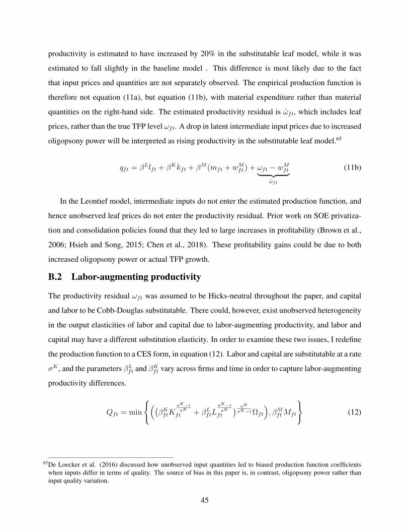
productivity is estimated to have increased by 20% in the substitutable leaf model, while it was

estimated to fall slightly in the baseline model . This difference is most likely due to the fact

that input prices and quantities are not separately observed. The empirical production function is

therefore not equation (11a), but equation (11b), with material expenditure rather than material

quantities on the right-hand side. The estimated productivity residual is ωft, which includes leaf

prices, rather than the true TFP level ωft. A drop in latent intermediate input prices due to increased

oligopsony power will be interpreted as rising productivity in the substitutable leaf model.65

qft = βLlft + βKkft + βM(mft + wMft ) + ωft − wMft︸ ︷︷ ︸ωft

(11b)

In the Leontief model, intermediate inputs do not enter the estimated production function, and

hence unobserved leaf prices do not enter the productivity residual. Prior work on SOE privatiza-

tion and consolidation policies found that they led to large increases in profitability (Brown et al.,

2006; Hsieh and Song, 2015; Chen et al., 2018). These profitability gains could be due to both

increased oligopsony power or actual TFP growth.

B.2 Labor-augmenting productivity

The productivity residual ωft was assumed to be Hicks-neutral throughout the paper, and capital

and labor to be Cobb-Douglas substitutable. There could, however, exist unobserved heterogeneity

in the output elasticities of labor and capital due to labor-augmenting productivity, and labor and

capital may have a different substitution elasticity. In order to examine these two issues, I redefine

the production function to a CES form, in equation (12). Labor and capital are substitutable at a rate

σK , and the parameters βLft and βKft vary across firms and time in order to capture labor-augmenting

productivity differences.

Qft = min

((βKftK

σK−1

σK

ft + βLftLσK−1

σK

ft

) σK

σK−1 Ωft

), βMftMft

(12)

65De Loecker et al. (2016) discussed how unobserved input quantities led to biased production function coefficientswhen inputs differ in terms of quality. The source of bias in this paper is, in contrast, oligopsony power rather thaninput quality variation.

45

Capital substitutability Still assuming profit-maximizing manufacturers, and deriving the first

order conditions, the equation to estimate the elasticity of substitution between labor and capital

is given by (13). There are two differences with equation (10b), which was used to estimate the

elasticity of substitution between leaf and labor. First, the capital market is assumed to be perfectly

competitive, so there is no markdown over capital prices that enters the residual. Second, there is

heterogeneity in the output elasticities of labor and capital, which reflects differences in labor-

augmenting productivity.

lft − (kft + wKft) = −σKwLft + (σK − 1)wKft − σK(

ln(βKft)− ln(βLft))

(13)

I estimate equation (13) using the same BLP instruments that were used in section B.1. The

estimated elasticity of substitution between labor and capital is in the right column of table A2,

and it estimated to be 0.918. This is very close to the elasticity of substitution of one imposed in

the baseline model.

Directed technical change Next, I test whether the consolidation induced factor-biased tech-

nical change. If the factor-augmenting productivity levels βLft and βKft changed in response to

the consolidation, for instance because consolidated firms upgraded their production technology,

this would threaten the interpretation of the markup and markdown results: the output elasticities

of labor and capital would not be invariant to the consolidation. From equation (13), it is clear

that the capital-labor ratio would then have to change in response to the consolidation. I test this

by estimating the difference-in-differences equation (1) with the capital stock per employee ratio

kft +wKft− lft as the left-hand side variable. The results are in table A4. The change in the capital

stock per employee was not significantly different between the firms in the treatment and control

group. The consolidation hence did not lead to factor-biased technical change.

B.3 Translog production function

The labor-capital substitution elasticity that was estimated in the previous section supports the

Cobb-Douglas assumption for the labor-capital term H(.) in the production function. In this sec-

tion, I nevertheless use a more flexible translog specification for H(.) as a robustness check. The

46

corresponding functional form of h(.) in logarithms is given by:

h(Lft, Kft) = βLlft + βKkft + βLK lftkft + β2Ll2ft + β2Kk2ft

I use the same identification approach as in the main specification. The moment conditions from

equation (9) are now adapted to:

E[υft|(lfr−1, kfr, lfr−1kfr, k

2fr, l

2fr−1, pfr, w

Lfr)]r∈[2,...,t]

= 0

I still include the instruments only up to one time lag, as in the baseline model. The resulting

estimates are in the right column of table A3. They are very similar to the baseline estimates.

B.4 Heterogeneous intermediate input requirements

The tobacco leaf content per cigarette, βMft , was assumed to be constant across firms and time. I

revisit this assumption using data on product characteristics for a sub-sample of firms. Variation

in cigarette characteristics, such as the leaf content per cigarette and filter density, is very limited

across manufacturers, as shown in table A1. The average manufacturer uses 683 mg of tobacco leaf

per cigarette of 1000 mg, and the standard deviation of this content is merely 30 mg. The entire

distribution of leaf contents lies between 630 and 750 mg. This range is much too small to explain

the observed decline in the leaf share of revenue. Moreover, as long as product characteristics are

similar between the control and treatment groups, they do not affect the difference-in-difference

estimates. Table A5(a) compares all product characteristics between the treatment and control

groups. Both groups did not differ in any of the observable characteristics, and barely any of the

variation in product characteristics is explained by the treatment dummies. Table A5(b) estimates

how markups, markdowns and productivity vary with the observable product characteristics. None

of the variables of interest correlates significantly with any of the product characteristics.

B.5 Non-profit maximizing firms

Assumption 2 stated that manufacturers maximize their per-period variable profits. As was dis-

cussed earlier, various industry sources confirm that cigarette manufacturers compete against each

other on their input markets and have incentives to lower their costs. More in general, Chen et al.

(2018) offers a detailed discussion and nuanced defense of the profit maximization assumption for

47

Chinese SOEs. Still, Chinese firms, and especially those that are state-owned, may optimize a

different objective function, such as ‘achieving social stability’ through high and countercyclical

employment (Li et al., 2012). In this section, I discuss two ways in which such size objectives can

enter the manufacturer’s profit function, and how this affects the model estimates.

Output size objective A first deviation from profit maximization could be that manufacturers

value being large, and are willing to sacrifice some profits to achieve higher output. This changes

marginal costs MCft: the additional cost of producing more is lower if manufacturers value being

large. Let the altered marginal costs be denoted MCft =MCftςft

. Manufacturers with a preference

for producing a lot have a parameter ςft > 1, and the more outspoken this preference is, the

larger ςft. Consistently with the markup expression used before, the true markup is now given by

µft = ςftPftMCft

. If manufacturers value being large rather than profitable, the true markup µft will

hence be larger than the estimated markup µ =PftMCft

. The reason for this underestimation is that

the cost minimization model infers large input usage as an indication of low markups, whereas in

reality, this is due to a preference towards large size. The same holds for the markdown ψMft : if

manufacturers value a large size, they will set higher input prices, even if they could drive input

prices further down by fully exerting their oligopsony power. The estimated markdown is hence

downward-biased if firms have a preference for being large.

Input size objective Now suppose that manufacturers specifically want to employ a lot of man-

ufacturing workers, but do not have such preferences for farming employment (or the other way

around). In this case, the true input price WLft is different from the measured input price. If manu-

facturers value employing many workers, the true price of labor is lower than the observed wage:

WLft = WL

ftςLft with ςLft < 1. As manufacturers do not choose labor and tobacco leaf separately, this

has the same effects on markup and markdown estimates as a different marginal cost. Marginal

costs are linear in both input prices, as shown in appendix D.3. If firms have a preference for em-

ploying many workers, the true markup and markdown are hence again an underestimate of their

true values.

Interpreting the consolidation treatment effects In sum, firm objectives that diverge from

static profit maximization lead to biased markup and markdown estimates. Even if these diverging

objectives would apply to this industry, this is not necessarily problematic for interpreting the esti-

mated consolidation treatment effects. First of all, only differences between manufacturers matter:

48

98% of the market is under some type of state control, so large differences in objective functions

are not that likely. Secondly, even if manufacturers differ in their objectives, this is not a problem if

their objective function is stable over time: such differences get absorbed in the manufacturer fixed

effects that were included in the difference-in-differences model. Finally, even if manufacturers’

objectives would change over time, this is fine as long as changes in manufacturers’ objectives are

uncorrelated to the consolidation treatment. It is unclear why the exit of competing manufacturers

would change the objective function of the incumbent firms.

B.6 Regulated leaf prices and pricing decisions

In theory, leaf prices and quantities were regulated in China until 2015, meaning that prices per

quality grade were determined by provincial STMA boards (Wang, 2013; Peng, 1996). In practice

there were, however, many ways in which manufacturers could choose leaf quantities and prices.

First of all, manufacturers can choose leaf prices by gaming the official quality grade to which

farmers’ leaves are attributed, as mentioned by (Peng, 1996). More formally, denote ζft the sub-

jective grade communicated by manufacturing firm f to its farmers, whereas the actual quality

grade is ζft. As leaf prices are a direct function of the subjective grade, WM(ζft), choosing the

subjective grade corresponds to choosing the leaf price, holding the true quality grade ζft fixed.

Second, the official grade-price schedules were determined by provincial STMA boards, but

these were populated by executives of the CNTC cigarette factories: the decentralized branches of

the industry regulator and manufacturing firms were de facto the same organization (Wang, 2013).

Firms can therefore adjust the official local leaf price per grade schedule through the decentralized

STMA boards. This does not imply that manufacturers could game all STMA regulations: the

policies set by the central STMA board, such as the consolidation policy, were not subject to the

authority of local STMA boards.

B.7 Leaf market definitions

Changing market definition in treatment effects Defining leaf markets is key to define which

firms are subject to the consolidation and which firms are not. In the main text, leaf markets were

defined at the prefecture level when constructing these treatment indicators. In table A6(a), I com-

pare the results when defining the treatment indicators using both province-level and prefecture-

level market definitions. Markdowns are estimated to increase by 26% when using the province

49

level treatment indicator, which is similar to the increase of 30% when defining treatment effects

at the prefecture level. The pattern of increasing markdowns hence holds across the various market

definitions. The fact that the estimate is the highest at the county level is not surprising: closer

manufacturers are likely to be closer competitors on leaf markets. As was explained before, the

markup drop is larger and significant at the province-level. The productivity change after the con-

solidation is, finally, not significantly different from zero across all different market definitions.

Changing market definition in the markdown expression Leaf markets also need to be defined

when estimating the markdown. In the baseline model, province-level market shares were used,

because the number of observations falls when defining narrower markets. In table A6(b), I com-

pare the estimated treatment effects when using prefecture-level and province-level market shares

to construct the markdown expression, and to define the treatment and control groups. Markdowns

are now estimated to increase by 46%, rather than by 30%, while the estimated markup change is

similar to the original specification.

C Production function identification: alternatives

C.1 Control function approach

In the main text, I combined the timing assumptions of Ackerberg et al. (2015) with the dynamic

panel approach of Blundell and Bond (2000), which relies on differencing out the persistent part

of the productivity residual. An alternative identification strategy is to rely on an inverted input

demand function to control for the latent productivity scalar (Olley and Pakes, 1996; Levinsohn and

Petrin, 2003; Ackerberg et al., 2015). In this section, I use this alternative identification approach.

Choice of the flexible input Intermediate inputs are usually used as the flexible input for the

first stage inversion. Oligopsony power over these intermediate inputs is problematic if interme-

diate inputs are substitutable with the other inputs. Persistence in oligopsony power would then

induce serial correlation in intermediate input prices, which are not observed separately from input

quantities, and hence violate the assumptions of Ackerberg et al. (2015).66 If intermediate inputs

are not substitutable and enter the production function with fixed proportions, as is the case in this

paper, intermediate input prices can be backed out by taking the ratio of material expenditure over

66Moreover, substitutable intermediate inputs would be subject to the identification problem for gross output productionfunctions highlighted by Gandhi et al. (2020).

50

output quantities, assuming that the intermediate input requirement is constant across firms and

time. I therefore use tobacco leaf as the flexible input for the first-stage inversion, and include the

leaf price as an argument in the first-stage regression, as explained below.

Input demand I derive the leaf demand function in appendix D.4. Leaf demand depends on the

cigarette price, the leaf price, and all other input prices and quantities. All these variables are either

observed or imputed from the data. Leaf demand also depends on the output elasticities of labor

and capital, the leaf requirement per cigarette, the markup, the markdown, and on productivity,

which are all latent.

mft = m(Pft,WMft ,W

Lft, Lft, Kft, β

L, βK , βM , ωft, µft, ψMft )

The leaf requirement βM and output elasticities βL and βK are assumed to be the same for all

firms and time periods. Markups, markdowns and productivity vary, however, flexibly across

firms and time. Without making further assumptions on the distributions of at least two of these

three variables, the scalar unobservable assumption is violated, and Ackerberg et al. (2015) is not

identified. High input demand can, namely, be due to high productivity, low markups, and/or low

markdowns.67

Ackerberg et al. (2015) can still be used if we impose additional assumptions on the markup

and markdown distributions. I impose a logit demand system for cigarettes similar to the one

assumed for leaf supply. Markdowns are still given by equation (6). Denoting the price elasticity

of demand as γP , which is assumed to be constant across firms and time, and the cigarette market

share as SQft, markups are given by:

µft =(γPPft(1− SQft)

)−1

+ 1

All variation in markups and markdowns is then captured by the observed cigarette and leaf prices

and the cigarette and leaf market shares. A similar assumption was made in De Loecker et al.

(2016) for settings in which there is only imperfect competition downstream. I therefore include the

leaf price WMft , cigarette price Pft, and market shares sft = (sQft, sft) in the first stage regression,

67Doraszelski and Jaumandreu (2019) make a similar point for markups, but does not allow for endogenous input prices.

51

which is given by equation (14). In contrast to the baseline model, there is now measurement error

in output εqft.

qft = φt(lft, kft, wMft , w

Lft, pft, sft) + εqft (14)

Productivity can now be recovered as a function of data and the estimable parameters, using

the same functional form assumptions that were made in the main text.

ωft = φft − h(lft, kft,β)− a(wLft, pft)

Moment conditions I retain the AR(1) equation of motion for productivity from equation (8b).

The productivity innovation υft is given by the difference between productivity and its expected

value from the equation of motion.

υft = ωft − E(ωft|ωft−1

)Keeping the timing assumptions from the main text, the moment conditions to identify β are

given by:

E[υft(lft−1, kft, wft, pft)

]= 0

When estimating this model, I use a third-order polynomial in all the inputs for the first-stage

regression. I block-bootstrap the standard errors with 50 iterations.

Results In table A7, I compare all estimates between the dynamic panel model from the main

text and the control function approach outlined above. The output elasticities are in panel A7(a).

The output elasticity of labor and capital are respectively higher and lower when using the control

function approach (‘ACF’) compared to the dynamic panel approach (‘BB’), but are not signifi-

cantly different from each other. The markdown and markup levels, in panels A7(b)-(c), are very

similar between both approaches, but the markdown estimates have much larger standard errors

when using ACF. The reason why markups are not very different in spite of the output elasticity of

labor being almost 50% higher is that labor costs are a small fraction of total variable input costs,

and are hence weighted with a small weight in the markup expression, (4a). The consolidation

treatment effects in panels A7(d)-(f) are very similar between both approaches, and lead to the

same conclusions about the effects of ownership consolidation.

52

ACF (2015) without first stage inversion Under the assumptions that intermediate inputs are

not substitutable and come in fixed proportions, and that intermediate input requirements βMft are

constant across firms and time, Ackerberg et al. (2015) suggest a simpler identification strategy

that does not require inverting the intermediate input demand function. One could simply back out

measurement error εqft up to a constant without having to invert the input demand conditions:

qft −mft = log(βM) + εqft

This approach is, however, not possible when intermediate input prices are both latent and en-

dogenous due to oligopsony power. Intermediate input prices are not separately identified from

measurement error, and are serially correlated if intermediate input market competition is persis-

tent:

qft −mft − wMft = log(βM)− wMft + εqft

C.2 Different productivity transition equations

The equation of motion for productivity implicitly rules out that the consolidation affected total

factor productivity, although such productivity gains were the official objective of the consoli-

dation policy. As an extension, I therefore allow the consolidation treatment dummies to affect

productivity directly. In contrast to Braguinsky et al. (2015); De Loecker (2013), which alter the

law of motion for productivity, I add the indicator of whether the firm was subject to the consol-

idation as an input to the production function. I assume that log productivity ωft has an AR(1)

component ωft, and a part that depends on whether the firm is in a consolidated market or not,

which is captured by the vector of dummies Zft:

ωft = βZZft + ωft

As was assumed in the main text, firms cannot choose whether they are subject to the consolida-

tion or not, so the variables Zft are exogenous. The equation of motion for the residual part of

productivity that is not explained by the consolidation follows equation (8b):

ωft = ρωft−1 + υft

53

The estimates of this alternative model are in table A8. The output elasticities of labor and capital

are very similar to those in the main specification in table 2. In line with the treatment effect

estimates in the main text, the consolidation did not lead to an increase in productivity, and even

slightly decreased firm productivity.

D Additional results and derivations

D.1 Quantity and price choices

When formulating the profit maximization problem in equation (3), it was assumed that firms

choose the output level that maximizes current profits. This problem can be rewritten as firms

choosing the leaf price which maximizes profits. From the production function, equation (2), we

know that output and leaf usage are proportional:

Qft = βMftMft

By inverting the inverse leaf supply function (5), leaf usage becomes a function of the firm’s leaf

priceWMft , quality ζft, and other characteristicsXft and ξft. Moreover, leaf usage is also a function

of these same variables of the firm’s competitors, which are indexed as −f :

Qft = βMftM(WMft , ζft, ξft,Xft,W

M−ft, ζ−ft, ξ−ft,X−ft, ;ψ

Mft )

By choosing its leaf price WMft , the firm therefore controls its output level Qft as well.

D.2 Measurement error

The model can be extended to allow for measurement error in output. Let the production function

be re-defined as follows, with the log of measurement error being εqft. I assume that this measure-

ment error is i.i.d. distributed across firms and over time.

Qft = minβMftMft,ΩftH(Lft, Kft,β)

exp(εqft)

54

The production function in logs becomes:

qft = h(lft, kft,β) + ωft + εqft

Rewriting the production function to take into account unobserved input quality differences gives:

qft = h(lft, kft,β) + a(pft, wLf,t) + ωft + εqft

The moment condition using the dynamic panel approach becomes:

E[υft + εqft − ρεqft−1|(lfr−1, kfr, pfr, w

Lfr)]r∈[2,...,t]

= 0

Using the dynamic panel approach, measurement error εqft and total factor productivity ωft are

not separately identified. If there would be measurement error in output, all statements in the

text about productivity hence apply to the sum of log productivity and log measurement error.

Furthermore, leaf prices are observed with error if quantities are observed with error: WMft =

WMftMft

QftβM exp(εqft). The productivity decomposition exercise, finally, also contains measurement

error in output:

Ωit ≡∑f∈Fit

(Ωft exp(εqft)

Fit

)

Ωit ≡∑f∈Fit

(Ωft exp(εqft)Lft∑f∈Fit(Lft)

)

D.3 Markup and markdown expressions

In this section, I derive the markup formula in equation (4a). Taking the first order derivative of

variable costs results in the following expression for marginal costs MCft:

MCft = WLft

∂Lft∂Qft

ψLft +WMftMft

Qft

ψMft

Substituting the revenue shares αVft ≡VftW

Vft

PftQft

for V ∈ L,M and βLft ≡∂Qft

∂Lft

LftQft

gives:

55

MCft =αLftPft

βLftψLft + αMftPftψ

Mft

Finally, dividing prices by marginal costs yields equation (4a).

D.4 Input demand function

I now derive the leaf demand function, which is used when identifying the production function

using Ackerberg et al. (2015) in appendix C.1. Using the maximization problem from equation

(3), the first order condition is:

∂Pft∂Qft

Qft + Pft −WLft

∂Lft∂Qft

−WMft

∂Mft

∂Qft

−∂WM

ft

∂Mft

∂Mft

∂Qft

Mft = 0

Using the Cobb-Douglas function in labor and capital for H(.), the optimal output level Q∗ft is

equal to:

Q∗ft =[(Pftµft−WMft

βMftψMft)βLω

1

βL

ft KβK

βL

ft

1

WLft

] βL

1−βL

From the production function, it can be seen that the optimal leaf level is equal to M∗ft =

Q∗ftβMft

.

In short notation, intermediate input demand is hence a function of cigarette and input prices,

capital, the output elasticities of labor and capital and the leaf input requirement, and of total factor

productivity, the markup and the markdown.

mft = m(Pft,WMft ,W

Lft, Kft, β

L, βK , βMft , ωft, µft, ψMft )

D.5 Market structure and leaf prices

In table A9, I regress log leaf prices log(WMft ) on dummies that indicate the presence of one,

two or three manufacturers at the province, prefecture, and county level. There is no systematic

relationship between leaf prices and market structure at the province and county levels. At the

prefecture level, however, leaf prices are 60% lower when there is just one manufacturer, 46%

lower when two manufacturers, and 40% lower with three manufacturers, compared to prefectures

with four or more firms. This is additional evidence for oligopsony power in this industry.

56

D.6 Bargaining model between manufacturers and wholesalers

The drop in factory-gate cigarette prices and manufacturer markups in reaction to increased market

concentration downstream is less intuitive than the rise of leaf price markdowns. This fact can,

however, be explained using a bargaining model with double marginalization. Let the factory-gate

cigarette price Pft be the outcome of a Nash bargaining game between each manufacturer and the

wholesaler. Let Γf ∈ [0, 1] denote the share of the total surplus received by the manufacturer: if

Γft is zero, the wholesaler gets all the surplus, if it is one, the manufacturer does, and if it is one

half, they get an equal share. Denoting the wholesale price of a cigarette produced by manufacturer

f as PWft , and total manufacturing costs as TCft ≡ WM

ftMft +WLftLft + Ift, the Nash product is

given by equation (15a).

Γft( PWft Qft − PftQft︸ ︷︷ ︸

Wholesaler’s profit

) = (1− Γft)( PftQft − TCft︸ ︷︷ ︸Manufacturer’s profit

) (15a)

Rewriting equation (15a) for the factory-gate cigarette price results in equation (15b), with average

manufacturer costs ACft ≡ TCftQft

.

Pft =(

1− Γft

)ACft + ΓftP

Wft (15b)

Factory-gate price change First, consider the effect of the consolidation on factory-gate cigarette

prices, by taking the first derivative of equation (15b) with respect to the consolidation dummy

Zft. The first term is negative: the consolidation leads to lower average manufacturer costs, as leaf

prices fall. The second term can be positive: the decrease in the number of manufacturers could

lead to higher bargaining power by the manufacturers downstream, which implies a higher Λ. The

third term is likely to be zero: wholesale market structure was not affected by the consolidation.

∂Pft∂Zft

=(

1− Γft

)∂ACft∂Zft︸ ︷︷ ︸

<0

+∂Γft∂Zft

(PWft − ACft)︸ ︷︷ ︸

>0

+ Γft∂PW

ft

∂Zft︸ ︷︷ ︸=0

Equation (15c) gives the condition under which the consolidation led to lower cigarette prices:

the drop in manufacturer average costs should be larger in absolute value than the increase in

57

bargaining power by the manufacturer on the wholesale market. As was shown in table 1(a),

factory-gate cigarette prices fell in response to the consolidation, which suggests that the condition

in equation (15c) holds in the tobacco industry setting.

∂Pft∂Zft

< 0⇔ (1− Γft)∂ACft∂Zft

< −∂Γft∂Zft

(PWft − ACft) (15c)

Manufacturer markup change Next, rewriting equation (4a), the manufacturer markup is given

by:

µft =Pft

WLftLft

βLQft+

WMft ψ

Mft

βM

The numerator of the markup expression, factory-gate cigarette prices, fell due to the consolida-

tion. Marginal labor costs, in the denominator, remained constant. The marginal cost of tobacco

leafWMft ψ

Mft

βMalso did not change much: although leaf prices fell by 35%, as shown in table 1(a),

leaf markdowns increased by 30%. As factory-gate cigarette prices fell, whereas manufacturer

marginal costs remained constant, manufacturing markups fell as well. As was explained earlier,

this does not mean that the manufacturing profits fell: manufacturers earn profits both from the

wedge between cigarette prices and marginal costs, and from the wedge between marginal costs

and leaf prices. Manufacturer variable profits increased as long as the increase in the leaf price

markdown was higher than the drop in the cigarette price markup.

D.7 Markdown and markup drivers

Which firm and county characteristics explain variation in markups and markdowns? In table A10,

I report some correlations. Leaf markdowns are larger in prefectures with one or two cigarette

firms, which is consistent with the classical oligopsony model. Markdown ratios are somewhat

higher in prefectures with a higher unemployment rate. Oligopsony power pushes down employ-

ment, and a high unemployment rate may also indicate less appealing outside options to farm-

ers, which contributes to the exertion of oligopsony power by cigarette factories. Markdowns are

higher in smaller firms, while markups are higher for larger firms. Taxes as a fraction of revenue

are higher for firms with high markdowns, which may indicate that the government extracts a part

of the oligopsony rents.

58

Table A1: Summary statistics

Mean S.D. Obs

Revenue (million $) 109.71 206.17 1120

Quantity (thousand cases) 429.56 546.42 1120

Price per case ($) 529.61 1308.14 1120

Profit (million $) 13.27 48.25 1120

Wage bill (million $) 3.58 6.26 1120

Material expenditure (million $) 36.92 53.97 1120

Capital stock (million $) 49.87 76.90 1120

Employees 1208.60 1096.89 1120

Export dummy 0.23 0.42 1120

Export share of revenue 0.01 0.05 1120

Prefecture population (millions) 1.19 1.39 1120

Leaf content per cigarette (mg) 683.46 31.55 181

Filter density (mg/ml) 112.79 3.62 181

Notes: A case contains 50,000 cigarette sticks. Prices are factory-gate prices. Revenue, prices, profits, and inputexpenditure are denoted in 1998 US dollars.

59

Table A2: Input substitution elasticities

Labor and leaf Labor and capitalEst. S.E. Est. S.E.

Elasticity of substitution -0.002 0.291 0.918 0.210

1st stage F-stat 39.24 39.24

R-squared 0.281 0.465

Obs. 1,120 1,120

Notes: This table reports the substitution elasticities between labor and materials, estimated using equation (10b),and between labor and capital, estimated using equation (13). Controls include ownership and CIC product dummies,

year dummies, export dummy and the export share of revenue, and log prices. Both the average export share ofrevenue and average export participation of other cigarette manufacturers within the same prefecture as used as

instruments for wages.

60

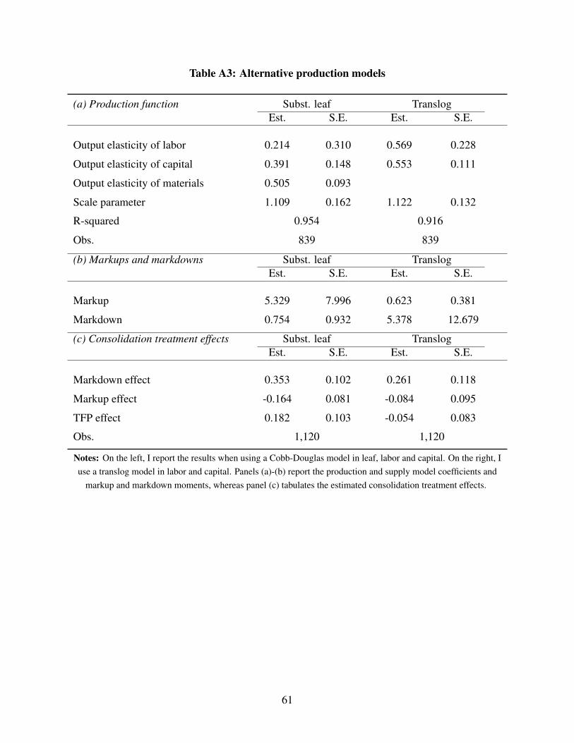
Table A3: Alternative production models

(a) Production function Subst. leaf TranslogEst. S.E. Est. S.E.

Output elasticity of labor 0.214 0.310 0.569 0.228

Output elasticity of capital 0.391 0.148 0.553 0.111

Output elasticity of materials 0.505 0.093

Scale parameter 1.109 0.162 1.122 0.132

R-squared 0.954 0.916

Obs. 839 839

(b) Markups and markdowns Subst. leaf TranslogEst. S.E. Est. S.E.

Markup 5.329 7.996 0.623 0.381

Markdown 0.754 0.932 5.378 12.679

(c) Consolidation treatment effects Subst. leaf TranslogEst. S.E. Est. S.E.

Markdown effect 0.353 0.102 0.261 0.118

Markup effect -0.164 0.081 -0.084 0.095

TFP effect 0.182 0.103 -0.054 0.083

Obs. 1,120 1,120

Notes: On the left, I report the results when using a Cobb-Douglas model in leaf, labor and capital. On the right, Iuse a translog model in labor and capital. Panels (a)-(b) report the production and supply model coefficients and

markup and markdown moments, whereas panel (c) tabulates the estimated consolidation treatment effects.

61

Table A4: Factor-biased technological change

log(Capital/employee)Est. S.E.

Treatment*1(Year≥2002) 0.025 0.041

Within R-squared 0.0914

Observations 1,120

Notes: This table estimates the effect of the ownership consolidation on the capital stock per employee, which is anindicator for labor-augmenting technological change. Firm fixed effects are controlled for.

62

Table A5: Product characteristics

(a) Comparisons log(Leaf weight) log(Filter density) log(Rod density)Est. S.E. Est. S.E. Est. S.E.

Treatment -0.001 0.013 0.007 0.008 -0.012 0.013

Obs. 286 286 286log(Paper permeability) 1(Ventilation)Est. S.E. Est. S.E.

Treatment -0.001 0.045 -2.190 2.179

Obs. 286 286(b) Correlations log(Markdown) log(Markup) log(TFP)

Est. S.E. Est. S.E. Est. S.E.

log(Leaf weight) -1.783 1.713 2.800 2.963 -4.477 3.448

1(Ventilation) 0.009 0.016 -0.002 0.023 0.031 0.040

log(Rod density) 2.555 2.640 -1.266 3.741 3.541 6.172

log(Filter density) -0.538 2.178 3.493 2.478 -1.434 4.749

log(Paper perm.) 0.252 0.858 0.226 0.701 -0.642 1.261

Obs. 181 181 181

Notes: Panel (a) compares the cigarette contents between the treatment and control groups. Panel (b) reports thecorrelations between markups, markdowns, productivity and cigarette characteristics. Standard errors are

block-bootstrapped with 50 iterations.

63

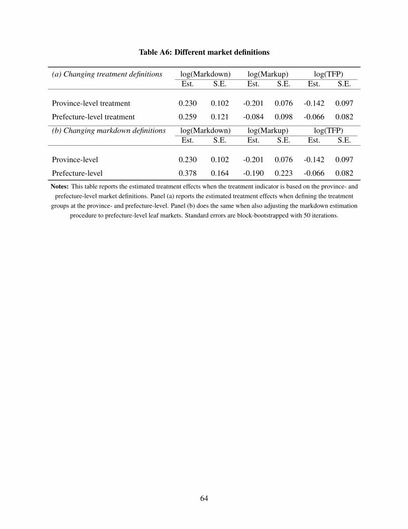
Table A6: Different market definitions

(a) Changing treatment definitions log(Markdown) log(Markup) log(TFP)Est. S.E. Est. S.E. Est. S.E.

Province-level treatment 0.230 0.102 -0.201 0.076 -0.142 0.097

Prefecture-level treatment 0.259 0.121 -0.084 0.098 -0.066 0.082

(b) Changing markdown definitions log(Markdown) log(Markup) log(TFP)Est. S.E. Est. S.E. Est. S.E.

Province-level 0.230 0.102 -0.201 0.076 -0.142 0.097

Prefecture-level 0.378 0.164 -0.190 0.223 -0.066 0.082

Notes: This table reports the estimated treatment effects when the treatment indicator is based on the province- andprefecture-level market definitions. Panel (a) reports the estimated treatment effects when defining the treatment

groups at the province- and prefecture-level. Panel (b) does the same when also adjusting the markdown estimationprocedure to prefecture-level leaf markets. Standard errors are block-bootstrapped with 50 iterations.

64

Table A7: Comparing ACF (2015) and Blundell-Bond (2000)

(a) Production function BB ACFEst. S.E. Est. S.E.

Output elasticity of labor 0.591 0.201 0.820 0.319

Output elasticity of capital 0.592 0.119 0.482 0.184

Scale parameter 1.182 0.094 1.302 0.144

(b) Markdowns BB ACFEst. S.E. Est. S.E.

Mean 5.307 3.237 5.396 17.874

Median 4.379 2.483 4.449 3.346

(c) Markups BB ACFEst. S.E. Est. S.E.

Mean 0.637 0.478 0.643 0.353

Median 0.526 0.475 0.527 0.614

(d) Markdown treatment effect BB ACFEst. S.E. Est. S.E.

Treatment*1(Year≥ 2002) 0.259 0.121 0.261 0.145

(e) Markup treatment effect BB ACFEst. S.E. Est. S.E.

Treatment*1(Year≥ 2002) -0.084 0.098 -0.082 0.115

(f) TFP treatment effect BB ACFEst. S.E. Est. S.E.

Treatment*1(Year≥ 2002) -0.066 0.082 -0.062 0.082

Notes: This table compares markdowns, markups, and all treatment effects between the Blundell-Bond (2000)model, on the left, and ACF (2015) on the right. Standard errors are block-bootstrapped with 50 iterations.

65

Table A8: Production function with consolidation as input.

log(Output)Est. S.E.

Output elasticity of labor 0.567 0.060

Output elasticity of capital 0.586 0.047

Treatment*1(Year≥2002) -0.070 0.032

Treatment -0.157 0.082

1(Year≥2002) 0.077 0.062

R-squared 0.917

Obs. 839

Notes: This table shows the production function estimates when inserting the consolidation treatment variables asproductivity shifters in the production function. Standard errors are block-bootstrapped with 50 iterations.

66

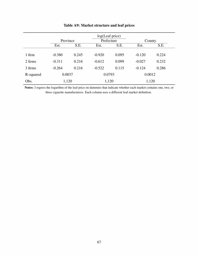
Table A9: Market structure and leaf prices

log(Leaf price)Province Prefecture County

Est. S.E. Est. S.E. Est. S.E.

1 firm -0.380 0.245 -0.920 0.095 -0.120 0.224

2 firms -0.311 0.216 -0.612 0.099 -0.027 0.232

3 firms -0.264 0.216 -0.522 0.115 -0.124 0.286

R-squared 0.0037 0.0793 0.0012

Obs. 1,120 1,120 1,120

Notes: I regress the logarithm of the leaf price on dummies that indicate whether each market contains one, two, orthree cigarette manufacturers. Each column uses a different leaf market definition.

67

Table A10: Market power correlations

log(Markdown) log(Markup)Est. S.E. Est. S.E.

1(SOE) -0.023 0.172 -0.064 0.172

log(Revenue) -0.090 0.038 0.164 0.026

log(Unemp. rate) 0.123 0.086 -0.196 0.082

log(Tax/Sales) 0.259 0.110 -0.093 0.087

log(Migration rate) -0.065 0.100 0.124 0.100

log(No schooling rate) -0.043 0.109 -0.019 0.105

1(# Firms = 1) 0.459 0.198 -0.356 0.195

1(# Firms = 2) 0.281 0.153 -0.151 0.155

1(# Firms = 3) 0.203 0.154 -0.220 0.155

R-squared 0.176 0.204

Obs. 776 776

Notes: This table regresses log markdowns and log markups on a selection of firm and market characteristics.Markets defined at the prefecture level.

68

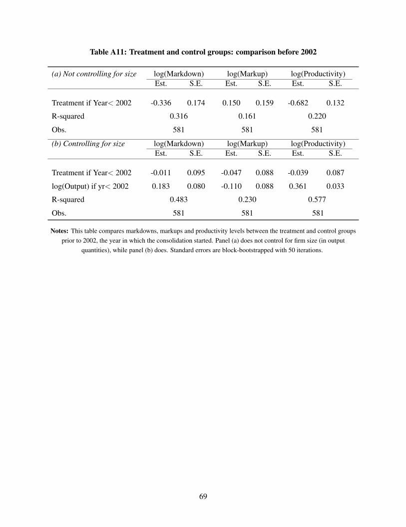
Table A11: Treatment and control groups: comparison before 2002

(a) Not controlling for size log(Markdown) log(Markup) log(Productivity)Est. S.E. Est. S.E. Est. S.E.

Treatment if Year< 2002 -0.336 0.174 0.150 0.159 -0.682 0.132

R-squared 0.316 0.161 0.220

Obs. 581 581 581

(b) Controlling for size log(Markdown) log(Markup) log(Productivity)Est. S.E. Est. S.E. Est. S.E.

Treatment if Year< 2002 -0.011 0.095 -0.047 0.088 -0.039 0.087

log(Output) if yr< 2002 0.183 0.080 -0.110 0.088 0.361 0.033

R-squared 0.483 0.230 0.577

Obs. 581 581 581

Notes: This table compares markdowns, markups and productivity levels between the treatment and control groupsprior to 2002, the year in which the consolidation started. Panel (a) does not control for firm size (in output

quantities), while panel (b) does. Standard errors are block-bootstrapped with 50 iterations.

69

Figure A1: Annual firm size distributions, pre-consolidation.

02.

000e

-06

4.00

0e-0

66.

000e

-06

Pro

babi

lity

dens

ity

0 100000 200000 300000 400000Annual output in cases

1999 20002001

Notes: This graph plots the distribution of the number of cigarette cases produced per firm in 1999, 2000and 2001, for firms producing less than 400,000 cases. There is no evidence for ‘bunching’ just above theexit threshold of 100,000 cases or the merger threshold of 300,000 cases, so self-selection into the groupjust above these tresholds is unlikely.

70