market value measures: duration analysis and …...want to hear about book value; they want to hear...

1997 VALUATION ACTUARY SYMPOSIUM PROCEEDINGS

SESSION 17

Market Value Measures: Duration Analysis and Economic Surplus

Frederick W. Jackson, Moderator

David N. Becker

Cindy L. Forbes

Douglas A. George

M A R K E T VALUE MEASURES: DURATION ANALYSIS AND E C O N O M I C SURPLUS

MR. F R E D E R I C K W. JACKSON: For some time now, we've had market value measures having

asset/liability management uses. Duration is a measure that's used to provide information to

portfolio managers about the interest rate sensitivity of their financial instruments. It 's also used on

the liability side. The definition of duration is the percentage change in market value given a 100-

basis-point shift in interest rates. We're going to talk a good bit about duration. Economic value

surplus is also a very commonly used market value measure. It's the difference between the market

value of assets and liabilities. Despite the widespread use of these different market value measures,

there remains a great deal of controversy surrounding their use. There has been a lot written on their

appropriate and inappropriate uses. Market value measures are actively traded in the investment

community. We don't have a similar type of situation on the liability side of the balance sheet.

Everybody knows about the treatment of Financial Accounting Standard (FAS) 115 where there's

different accounting treatment in the Annual Statement for assets classified as held to maturity

versus available for sale or actively traded. The fact that there is really no comparable treatment for

liabilities seems ludicrous. At Session 1, Donna Claire mentioned that there is some more noise

coming out of the FASB to revisit these issues.

What I 'm going to do now is introduce our panel. I think we'll have lively presentations fi'om them.

We are fn'st going to hear from Doug George. Doug is a partner at Avon Consulting Group. He has

done quite a bit on liability management issues, and he's a regular speaker at these sessions. Cindy

Forbes is vice president of risk management at ManuLife. She's responsible for asset/liability

management and market risk management. Our last speaker who 's going to wrap it up is David

Becker. Most of you are familiar with David, who is the chief actuarial officer and appointed

actuary for Lincoln National. He is a leader in research in this area. I 'm going to turn the session

over to Doug now.

MR. DOUGLAS A. GEORGE: As Rick mentioned, this topic is subject to quite a bit of debate

within our profession. The usefulness, or lack thereof, of market value type measures is quite a bit

379

1997 VALUATION ACTUARY SYMPOSIUM

controversial. I think there are some very knowledgeable people who will tend to swear by book

value type approaches and others swear more by market-value approaches. I think that says

something about these issues. It says that there is no black and white answer when it comes down

to book value versus market value. I think the real answer is that there are advantages and

disadvantages to both, and maybe finding those and making sure you're aware of those is the best

way to deal with these issues.

I want to begin by addressing book and market value measures in general. I ' ll present some of the

advantages and disadvantages and then get into some of the misconceptions that I believe surround

market value type measures. Let's discuss book value versus market value. I guess the bottom line

question is which one is the reality? I think some of the different measures are realistic in some

ways and unrealistic in others. We start with statutory measures, and statutory measures are

obviously designed for solvency. There's an inherent level of conservatism built into our statutory

reserving and our accounting. We have statutory reserves and policy reserves. We have interest

maintenance reserve (IMR) and asset valuation reserve (AVR) that we layer on top of this. We have

risk-based capital requirements on top of that as well. The nature of statutory accounting is really

to be conservative to make sure that companies maintain solvency. So they're not going to be

completely realistic when it comes down to the true economic picture of a block of business or a

company.

When we go to GAAP measures, I think you could say that GAAP does a little bit better job or gets

a little bit closer to economic reality, but perhaps it doesn't quite get there. You have FAS 60

business where we have provisions for adverse deviations that are built into our assumptions so that

they are slightly conservative, and not completely realistic. We also have assumptions that are

locked in so that if the nature of a block changes, the projections and the forward projections on the

business don' t really change, so the expectations on the business don't change. You have FAS 97

business where we do have a locking, but I think many of us, in our FAS 97 business, don' t unlock

when we should. Many of us have gotten to a point where we have a certain set of assumptions that

380

M A R K E T VALUE M E A S U R E S

we use for FAS 97 and for GAAP, but they are not quite the realistic assumptions that we expect for

that block of business. So the GAAP projections still aren't capturing the reality.

As Rick mentioned, we have FAS 115 where we have the assets marked to market and our liability

is staying at book value. I think this sort of inconsistent treatment makes the result very unrealistic.

If we move to market values, the intent would be to try to get a truer picture, but then we run into

other concerns that pertain to assumptions. Market values of liabilities are built around assumptions.

They're built around policyholder behavior assumptions of which none of us are completely sure.

They're built around projections of the liabilities as if they're assets. We treat them as securities and

use discount methods that come up with the present value. There's a big controversy over what the

appropriate discount rate is. Since there is no active market for trading liabilities and products, we

wonder whether we can get the appropriate discount rate. We can't reconcile it, we can't tag it, and

we can't calibrate it to a current market value since we don't know what the market value is.

Let 's move on to volatility. Volatility is a big concem with market values. Our book value is

designed to produce a steady, stable pattern of earnings and performance if it can. The people that

are looking at it from the outside really like to see a stable and steadily increasing pattern of

earnings, but market values just don't behave in that way. We get a lot of volatility, we get a lot of

ups and downs, and that type of pattern is just undesirable from an earnings standpoint.

Finally, there's communication with our investment people. Our investment people don't want to

understand book values or maybe they just claim they don't understand them. They really don't

want to hear about book value; they want to hear about market value. It 's tough to go to our

investment people and say, "Well, we have a single premium deferred annuity (SPDA) block that's

very interest sensitive, and we have a universal life block that is less sensitive. We also have a

traditional block that's not very sensitive, so please invest accordingly." You really need some sort

of measures and some sort of guidance for your investments behind blocks of business. Market

values, durations, and convexities can provide this method of communication, and if we ' re going

381


to really do asset/liability management, we really do need to get that communication going with the

investment people.

Let me give you a few quick examples of some market value versus book value calculations. I 'm

starting with a cash-flow-testing example so this is something that's very familiar to us. I 'm going

to show you some results from an actual block of SPDAs from the 1996 cash-flow testing. This is

a real case study, that shows some real "hot" SPDA money. We have a very simple definition of

economic surplus. This is our cash-flow-testing definition for market value of assets less our cash

value of liabilities. In Chart 1, we start with a positive economic surplus coming out of the box, and

interest rates in previous years have been decreasing so we have an unrealized capital gain that's

built up inside our asset portfolio. In cash-flow testing, we start with a zero statutory surplus, and

that's due to cash-flow testing. It looks like it's a little bit positive, but I think that's just an error

because we've been using a September 1996 start date and we're looking at the end of 1996 start

value on the charts so the starting statutory accounting is plus a zero on all these cases. Over the ten

years, we earned some spreads on the business and that produced statutory earnings. We earned our

normal spread or what I call our normal spread because we have a nice friendly interest rate scenario

and that produces earnings.

We also earned a higher yield and a higher spread due to the unrealized capital gains in the asset

portfolio. Over time, those gains are released in the form of higher spreads and flow through to

statutory earnings so that increases the earnings as well. By the end of the tenth year, the statutory

surplus is increasing and the economic surplus is at about the same spot. The economic surplus is

slightly higher because we used the cash value rather than a statutory reserve as the definition of

liability. The general idea is the economic surplus and statutory surplus ended up in the same spot,

and the economic surplus really was part of a driver for bringing the statutory surplus up. The

economic surplus showed me the direction that the statutory surplus is going, and the economic

surplus started out at a higher level, and it slowly released that surplus into statutory surplus over

time. You could buy that argument or maybe not. On the other hand, I have some nice statutory

382


earnings here and they really produce my statutory surplus. So maybe this argument doesn't work

so well under our level interest rate scenario or maybe we shouldn't be so worded about it.

C H A R T 1

Level Interest Rates (Scenario 1)

U~

O I N

m * D

:S

180

140

100

60

20

-20

-60

-100

-140 I I I I I I I I I I

1996 1997 1998 1999 2000 2001 2002 2003 2004 2005

Statutory Surplus

Economic Surplus

Statutory Earnings . t

If we move to our pop-up scenario (Chart 2), we get a little different picture. Right off the bat,

we've had an instantaneous pop up of 3%, and our economic surplus dropped from $70 million to

about -$80 million. Initially, we get positive statutory earnings for a couple of years, and this is due

to the lapses that we get and the extra interest-sensitive lapses under our pop-up scenario. We

receive surrender charges on that business, and much of that business is still within the surrender

period so we still achieve some statutory earnings. When we get to the middle years of the

projection, and while the surrender charge effect is wearing off, we're in a position to credit a higher

rate on our liabilities than we can earn on our assets. We're getting negative spreads here, and the

statutory surplus or statutory earnings goes down accordingly. In the last couple of years, most of

our assets have rolled over and are now earning higher rates. Since they're eaming higher rates,

383


we're back in a position where we're starting to achieve some positive spreads. Statutory earnings

slowly get positive towards the end of the projection.

The economic surplus, on the other hand, pops down to the - $80 million, and slowly, as time goes

on, the asset portfolio rolls over and economic surplus begins to creep up. By the end of the

projection, our two values are very close to each other. Actually we failed the scenario in this case

because we end up at the end of the ten years and we're still in a negative position. The point is, the

statutory earnings in this case were an invalid predictor for the first couple of years. We were in a

position where the business, through shock interest rates, had deteriorated quite rapidly fight off the

bat, and our statutory earnings gave us the wrong impression. They were the wrong signal, whereas

the economic surplus showed us what the right signal was. It showed us that our position had

deteriorated quite a bit, and slowly, over time, it improves, but the statutory earnings were really

misleading.

180

140

100

60 C O --'- 20 l i

u~ -20

-60

-100

-140

CHART 2

Immediate Pop-Up (Scenario #4)

m

i l l i

- ¢ • *

i i I i i i i i i i

1996 1997 1998 1999 2000 2001 2002 2003 2004 2005

Statutory Surplus i i

Economic Surplus e

Statutory Earnings

384

MARKET VALUE MEASURES

In Chart 3, I 've shown scenario number three with the rising and falling. In this case, we have

positive statutory earnings for three years and as interest rates slowly rise, we can still achieve some

small spreads. We also get some interest-sensitive lapses, and once again earn those surrender

charges so we get some statutory earnings. In the middle years, rates have gone too high so we're

back to a position where we have the negative spreads and the statutory earnings to reflect that.

Finally, at the end, interest rates come back down, much of our portfolio has rolled over and is now

earning higher rates. We're in a position where we're earning very big spreads and the statutory

earnings bounced back up again. We have our economic surplus as well, which gives you the more

direct picture of what's happening and is virtually related to interest rate movement. If you look at

this closely, you can see that the economic surplus had become a predictor for where the statutory

surplus is going. If you looked at the economic surplus like a moving average and a time lag on the

economic surplus, you could see how you could get a line very similar to that statutory surplus. The

statutory surplus is basically following the economic surplus line, but it is doing so with a time delay

and in a moving average type of fashion. So while the statutory surplus and the statutory earnings

gave you the wrong signal for the first couple of years, the economic surplus is giving you a much

quicker signal as to where your business is going and what's really going on underneath.

180

CHART 3

Rising then Falling Rates (Scenario #3)

140

100

- 1 4 0 ~ 1996 1997 1998 1999 2000 2001 2002 2003 2004 2005

385

Statutory Surplus

Economic Surplus

Statutory Earnings A


My conclusion, in terms of economic measures and book measures, is that you need a combination

of the two, and the market value gives you a truer picture of what's really going on and what's

underlying your business and the real health of your business. On the other hand, the book value

measure shows you the constraints that your business has. We do live in a world where we have

accounting, risk-based capital, reserving, as well as the present constraints on our portfolios and how

we manage our business. We can't ignore book values; on the other hand, they don't give us the true

picture that the market value measures give you.

I showed a demonstration where I looked at economic measures and book value measures in terms

of outlining and analyzing alternative investment strategies at Session 4. My general approach is

to try to use a combination. The ways you put the market value measures to use should be decided

by how much asset/liability risk you're taking in your business. If you have no asset/liability risk

in your business, the market value measures don't give you much extra value, and they don't really

show you anything that you don't know. For example, let's say you sell a five-year GIC, a bullet

GIC, and you buy a five-year zero-coupon bond to back it. The market value measures are going

to move up and down when interest rates move in the same fashion. In my ideal world, you can

actually earn a profit by selling this and you can cover your expenses as well. You're not going to

gain anything by doing market value measures, and you're not going to see anything in the business

that you haven't already seen. You're perfectly matched and you're not taking any asset/liability

risk. In this case, you're not really going to need the market value measures, but as you move into

lines of business and assets and liabilities, where you are taking asset/liability risk, that's where the

market value measures become more important, and that's where they can really show you the real

health of your underlying business.

In the remainder of my time, I want to talk a little bit about some misconceptions of market value

analysis. One is that it's the same as duration matching. I 've heard a lot of people over the years

make comments like, "Things will be fine if we could just get our assets and our liabilities matched.

If we could have our durations matched, we'd really be in good shape." I don't necessarily buy that

386


as the optimal position. Duration matching is ideal in a lot of ways and for obvious reasons, but it

may not be the best position for our companies to be in.

Let 's discuss duration matching misunderstandings. First is using a MacCauley and modified

duration. Many of us do tend to use some of these numbers, but they just aren't appropriate for

interest-sensitive assets and liabilities. They work fine if there is no interest sensitivity and interest

rate risk; however, when we have option-laden instruments, they just don't give you the right

answer. Another misconception is liability length. I 've heard some people talk about having a

universal life portfolio with a duration of close to ten, and an SPDA portfolio with durations of five.

I think these people haven't done the analysis to see what the real durations are. They're not

defective durations because I think it's probably optimistic to think that durations are out that far.

Another misconception is the accuracy of a liability duration. If duration is 2.73, I 'm guilty of

making that assumption too because I do these calculations for people and that's what I tell them.

You're probably better off saying it's about 2.5-3 because that's probably the real level of accuracy

that we have when doing these duration calculations. So you don't want to read too much into them.

Finally, another misconception I've seen is to match duration, without heavily considering the other

risks that are involved. Many people will match duration but not think much about convexity or key

rate duration, for example. I think convexity is probably the one we're most guilty of ignoring.

Chart 4 shows a price behavior curve and what your assets and liabilities might look like. Here I 've

matched my duration above my zero point. My current yield curve and both my assets and my

liabilities have a duration of four, but I haven't matched convexities. As soon as interest rates move,

my durations are out of line. They are out of line by quite a bit, so I haven't really considered my

other risks. Recently, many of us have been guilty of this type of approach and have taken more

convexity risk. I know that as we've squirmed over the last year or two to get that extra yield out

of our portfolio, many people have taken on a lot more mortgage-backed securities (MBSs) and more

collateralized mortgage obligations (CMOs). They're really getting a lot of convexity risk in their

portfolio. Under a big interest rate move, this convexity risk can really come back to hurt you.

387


CHART 4

Price Curve

°%= o° A s s e t s ~

L,abll,t,e

=%

o.

I 0

D=4

D=4

Let's go back to duration matching. Chart 5 shows the average yield curve fi~om the last ten years.

Perhaps you have considered your convexity risk and your other risks. Or perhaps you didn't and

you just want to be duration matched, and you think that that's the fight position to be in. I 'll argue

that maybe that's not right and it probably isn't correct for most insurance companies. There are

many theories as to why the yield curve is upward sloping. I categorize them into two general

groups: one is based on the yield curve being a predictor of future interest rates. This is more otten

known as the pure expectations theory where we have market forces that buy and sell at different

positions on the yield curve. If there was any arbitrage opportunity in the yield curve, the market

would take care of it and the yield curve would move until there was no arbitrage opportunity

because this yield curve and any yield curve has an interest rate prediction embedded in it. I f you

follow the forward rates implied by that yield curve, you will see a prediction for future interest

rates.

So this first grouping of theories really says that's the prediction that the market believes will

happen. Since I don't want to try to make a guess that's different than the market, I should be

duration matched because I 'm buying into that prediction. The second group doesn't believe that.

388


The second group finds another reason why the yield curve is upward sloping, and I think there are

a number of theories such as market segmentation and liquidity theory. Also, just having a term

premium that's built into the yield curve might cause people to demand a higher return for taking

the extra risk of going out longer on the yield curve.

C H A R T 5

Average Yield Curve (1987-97)

9%

8%

7%

6%

5% 0 5 10 15 20 25 30

Let me show you what the applied forward rate is for this yield curve (Chart 6). This is a short-term

forward rate that's implied by that yield curve. So if that were the yield curve today, this would be

the prediction of short-term forward rates. Over the first year or two, the yield curve predicts that

the short term rate goes from about 5.6% up to 7.5% or so. For the rest of the 30 years, the

prediction goes up to about 8.5% or so. This is the prediction that's embedded in that yield curve.

389

1997 V A L U A T I O N A C T U A R Y S Y M P O S I U M

9%

C H A R T 6

Implied Short-Term Forward Rates

8%

7%

6%

5%

Time

When we say we need the duration match, we're implicitly saying that we buy into this interest rate

prediction. I don' t want to go longer out on the yield curve and pick up that extra yield that comes

with going longer because I feel like interest rates are going to move in this direction. Let me give

you an example.

Table 1 shows the rate relationship o f that average yield curve and the forward rates that it predicts.

The one-year term rate has a spot o f 6.14%, and the two-year term rate has a spot o f 6.62%. So that

produces a one-year forward rate or the one-year rate forward one year from now o f 7.10%

Term

T A B L E 1

Rate Relationship

Spot

6.14 6.62 6.87

Term

2 4 6

Spot

6.62 7.07 7.40

Forward

7.10 7.52 7.94

390


How can we use this? Well, say I have a cash flow that I need to pay one year from now. My first

choice is to duration match and go out and buy an instrument on the one year part of the yield curve.

I can earn 6.14%. My second choice is to buy the two-year term rate and get 6.62%. After the first

year, I must pay this cash flow. What most of us tend to do is rely on new premiums coming in to

pay this cash flow, and we continue to keep the instrument that was on our books and just earn what

we think is the higher rate. Alternatively, you could sell the instruments at that point in time and pay

your cash flow. Then you can take either a capital gain or loss. Let's look at what the opporttmities

are of doing those different things, and let's look at the capital gain and loss since that's more the

pure example of the real economics.

If you buy that two-year instrument and interest rates don't move, then you've won because you

bought out and you're earning 6.62%. One year goes by and you pay off your one-year debt and

then you sell the instrument. Not only do you earn the extra yield (the extra 50 or so basis points

over the fast year), but you sell the instrument at that point for a capital gain because you've got an

instrument that yields 6.62%. It's now a one-year instrument because one year has gone by, and the

one-year term rate is only 6.14%. So not only did you get the extra 50 basis points for the first year,

but you received a capital gain as well. Naturally, if interest rates go down, you wouldn' t do that,

and that's the game that most of us have been playing for the last ten or twelve years. Interest rates

have been coming down, and we 've been mismatching duration. We've been going very long and

we've been winning real big. You can't continue to do that forever because interest rates cannot go

down forever, but that is how the industry has made a lot of money for the last few years.

Finally, interest rates can go up and that's obviously where your risk is, but the forward rate shows

you how far interest rates have to go before you lose by taking this bet. I f you buy that two-year

instrument and rates go up to 7.1% over that one-year period, you still haven't lost by going out and

buying the two-year instrument. You bought that two-year instrument, you earned your 6.62% for

the first year, and if you sold it at that point in time, you would have to sell it for a capital loss. The

capital loss would exactly offset the difference between the 6.62% and the 6.14%, so from an

economic standpoint, you'd be indifferent about doing this. So interest rates would actually have

391


to go higher than the 7.1% in order for you to lose if you play this game. I picked what is probably

the easiest example to show this. As you go further out on the yield curve, this relationship gets

tougher to win. Interest rates have to move less over a longer period of time than 1%. For instance,

if you go down to the three-year and six-year rate, you get about the same relationship, but in the

equivalent example, you'd have to bet on the interest rate staying within 1% of the starting rate for

over a three-year period rather than over a one-year period. The bottom line is this is the game that

we play, and we can win it, but we do need to be careful. As you go farther out on the yield curve,

it gets a little bit tougher. The advantages aren't as big as they were in the example I pointed out.

In today's interest rate environment, the yield curve is somewhat flatter than it has been historically.

This game is definitely getting tough and that's why we are moving towards taking more convexity

risk.

When all is said and done, I think Chart 7 is the kind of profile that we ' re faced with. When I say

a duration match approach, I mean a full hedge position because that's what I think many of us mean

when we say we need to be duration matched. We really mean we think we should be fully hedged.

We want our assets and liabilities to go up and down in unison with the way the interest rates move.

Oftentimes we end up in a position where we can do that, but we really don't get the expected return

that we need. Many times we end up with some degree of mismatch that is going to be the optimal

position where we can get an expected return that's decent or at least reasonable with an appropriate

level of risk.

If you continue to go farther out on the yield curve and mismatch too much, you're going to end up

in a position where you can get a higher expected return. The degree of risk that you're taking is just

too high to keep playing that game. This is what many of us do. We have a mismatch in our

asset/liability portfolios, and whether we realize it or not, it's there for most of us. We're somewhere

around this mismatch point were we have a reasonable degree of mismatch. Hopefully we haven't

taken too much risk to the point of threatening the solvency of our company. We take the risk

because of the nature of our industry. We are in a very highly competitive industry; we can afford

to take this risk, and we do take it. Because we can afford it and our competitors can afford it, we

392


need to do it in order to keep up with them. I think it's part of the lesson of modem portfolio theory

that you really need to diversify your risks; duration risk is one of them. We have a number of other

ways that we take risk, and the best thing that most of us can do is try to diversify among the

different categories and among the different ways that we take risk as companies. You want to

spread your risk out, and that's really the lesson to be learned and that's the position of our industry

today. Take risk, spread it out, quantify it so you know you are not taking too much. Keep tabs on

it. This applies to duration as well as other risks and this is why duration matching is not usually

the optimal risk/reward profile.

C H A R T 7

Risk/Reward Profile

E

u~

Large Mismatch

M a t c ~

Risk

MS. CINDY L. FORBES: I think that Rick asked me to speak so I could be the controversial one

on the panel. Rick knows from our work on the SOA Asset/Liability Management Principles Task

Force that I 'm a strong proponent of economic values as being the driver. He also knows that Dave

is a strong proponent of statutory income and that Dave's position is more in line with other U.S.

393


actuaries. My comments today are going to start with a discussion of why I don't believe statutory

should be the driver; then I'll carry on with a high-level overview of how I would select asset/

liability management tools and techniques based upon the problem I 'm trying to solve. I believe

very much that the problem you're trying to solve drives the measures you use. Because not every

problem is a nail, you need to have more than a hammer in your toolkit.

I think you'll find that both Dave and I are rather passionate about our views. I think that's because

we have somewhat different belief systems and belief systems always lead to passion. So to begin

with, why are our views different? My company and I have a very strong belief that it's our job to

maximize the long-term economic value of the company. The economic value in our definition isn't

necessarily market value; it's how much money you have left after you pay off for your liabilities

given whatever investment strategy you're following for both the basic liabilities as well as for

surplus. Now that doesn't mean that we completely ignore the emergence of statutory income. We

recognize that there are very real internal and external constraints that we have to take into

consideration. The first one that we look at, and that is quite real to us, is earnings volatility. We

recognize that external stakeholders do not reward you for having extreme earnings volatility year

to year. There is a premium that is given to companies who demonstrate stable earnings over time.

We take that into account in our analysis. Capital availability is another constraint, as reflected in

minimum regulatory capital ratios. Internal return on equity (ROE) or return on assets (ROA)

targets are further examples of constraints.

You must also consider the timing of net statutory income emergence. For example, in Canada,

realized and unrealized stock gains are amortized into income at 15% per year. Thus increasing

stock holdings results in a drag on statutory income as the dividend income on the stock plus the

amortized gain is less than a bond return. Therefore, another constraint we impose when solving for

an appropriate investment strategy is the reduction in statutory income initially.

The actuarial paradigm in Canada is very much based on economic value. We build up reserves

starting with best-estimate assumptions for all of the parameters underlying the valuation of a

394


liability. This is similar to a gross premium valuation. Then for each assumption or experience

variable, we add a provision or margin for adverse deviation. This results in a direct link between

our reserves and the economic value of the company. Our margins for adverse deviation represent

the present value of future statutory income on the in-force business.

My position is not that statutory income is irrelevant but that the objective function for asset/liability

management purposes should be to maximize economic value subject to a number of constraints,

of which statutory income is but one.

I believe this because the constraints and statutory income impacts across lines of business will tend

to offset each other, and therefore you will get a suboptimal total result if you optimize each piece

using statutory income or the emergence of statutory income as the objective fimction. We feel very

strongly that if, in our analysis, we identify an investment strategy that creates long-term value for

the company but impairs stastutory income to a significant degree, we should look very hard for

ways to manage our affairs to obtain the best of both, i.e., capture the value without impairing

statutory income.

So I think the primary reason I don't agree wholeheartedly with Dave is because I don't like to

constrain my decision set by just looking at what drives statutory income; I want to look at the full

range of outcomes. Then, if I have a strategy that gives me as good a return from a point of view

of statutory income but gives me more economic value, I want to look at that and see what I can do

to unlock some of that hidden value in my statutory results. There are a number of ways you can

manage your balance sheet to unlock hidden value. Leverage and selected asset sales are common

tools available.

Second, optimizing your investment strategy based on statutory income and the release of regulatory

capital causes decisions to be based on, in essence, arbitraging the rules embedded in statutory

accounting and RBC. Personally, I don't believe that these rules are sufficiently well grounded for

395


me to run my business by finding solutions that optimize these results. Statutory accounting and

RBC rules are not in tune with economic reality.

Let 's take a company that has gross premium reserves that are a certain percentage of total assets.

It has a certain amount of its assets tied up to support statutory margins. It has set aside some money

to cover the interest valuation reserve (IVR), the asset valuation reserve (AVR), and the interest

maintenance reserve (IMR), and it has a certain amount of required statutory surplus, i.e., surplus

in excess of that required to meets its target RBC. You must have assets that are appropriate to

match your liabilities for your gross premium reserves, and you must take into account the fact that

you're going to have to set aside assets to support statutory margins. However the investment policy

for assets supporting statutory margins may be invested more aggressively, especially if you feel the

statutory results for the line of business are excessive. Assets also need to be set aside to cover the

AVR and the IMR. However the IMR simply is set up to hold back capital gains realized on bond

trading -- gains largely due to changes in interest rate levels. Required surplus is a cost of doing

business. However the target RBC level is somewhat soft. This is hardly a driver of asset strategy.

Would you not do an investment strategy that provides superior economic value because it drives

you from a 250 RBC to 230? There is a cost to a lower RBC ratio, but it 's not a hard constraint.

That's why I prefer to look at the problem across the entire balance sheet. If I have an investment

strategy that penalizes statutory income emergence or my capital ratio but provides enhanced

economic value, I see what options I have to manage around it. Keep in mind that statutory income

versus economic value is only a timing difference. For that reason, you must always run your model

until all the business lapses, in order to ensure all timing differences reverse.

In summary, we believe that it's our job to get the maximum value out of our balance sheet, and we

should not be driven by externally imposed constraints. We look at them seriously, but we try not

to have them be the drivers of our business decisions.

Now I want to talk about what kind of tools to use for different kinds of asset/liability management

problems, and there are three kinds of problems that I see running through all kinds of ALM work.

396


The first is a common one: either reevaluate the strategy you have or look at a strategy for a new line

of business. Second, you have your strategy, but your asset managers want to know how to invest

new cash flows or disinvest to pay liability obligations. A related problem is evaluating the

performance of your asset managers. The third kind of problem is setting risk limits. How much

risk will you let your managers take on your behalf, and will you tell them and senior management

how much risk they actually have on the books relative to their limits. I 'm going to start by talking

about the kind of tools you use when you're developing investment strategies and what the

considerations are.

When evaluating an investment strategy for a line of business, the tool you need is an asset model

that develops the terminal value of the business under different investment strategies. Outputs from

the model should include annual statutory income and required capital in addition to terminal value.

This assumes that you have a line of business that has a certain amount of optionality either on the

asset side, the liability side, or both. If you have a fixed stream of liability payments, obviously you

can just match up your assets to your liabilities.

The second kind of problem is investment direction and benchmarks. As I said, this means how do

I invest and how do I disinvest? When has the investment manager done a good job for me? The

challenge here is having congruency between the investment manager (believing that he has done

a good job) and the company (actually having achieved superior economic value). There are always

compromises. It's just like on the accounting side where you're looking at whether or not you

should be marking your liabilities to market value using asset techniques. The bottom line is, you

always run into problems because liabilities are like assets. They're not assets. As a result, you're

always forced to make assumptions and go into a world where it's not clear how you should be

translating the liabilities into asset terms or the assets into liability terms.

Solutions to the investment direction and benchmark problems range from total rate of return

measures based on external benchmarks such as Lehman Brothers to internally created benchmarks

that match the liabilities. You need to choose an internally created benchmark if the profile of the

397


liabilities is such that you can't find a suitable extemal benchmark, for example. Intemally created

benchmarks have their drawbacks. You have to set asset return assumptions. For example, will you

be investing your internal benchmark in corporate A bonds, or will you be investing in triple B

bonds? What are the spreads over Treasuries for those kinds of bonds? Can your asset managers

find those kinds of bonds on a particular day? Clearly manpower is an issue as well. Creating

internal benchmarks takes time and effort to maintain, and there's always a timeliness issue. You

have a new liability profile and then you have to update your benchmark profile before your asset

managers can take any action. These are the kinds of issues you have to deal with when you're

selecting or creating benchmarks, but it's important that you give it a lot of thought because

obviously you want to have the goals of your managers congruent with the overall goals of the

business.

Another way of approaching investment benchmarks and benchmark direction is simply to use a

spread model, reward your managers for achieving a certain spread over the liability required rate

or over Treasuries, for example. That may align both the asset and liability side with the short-term

objectives of the business, but it may not incent them to manage credit or option risk proactively.

The final method is simply rewarding managers on the present value of the spread earned on the

assets to the liabilities. It does take into account the entire impact of an investment decision but

values the impact on a liability basis.

Problems specific to external indices include: a) how they are only able to match overall duration

of liabilities, and b) profile of how external indices change over time with market issuance. Internal

benchmarks require you to take the liabilities and translate them into assets. That's not necessarily

difficult, but it is time consuming and it certainly takes more manpower. It also is assumption

driven. If you have liabilities that have a lot of embedded options, you probably can't find notional

assets that are going to replicate the liability profile.

The obvious problem with using a spread approach to rewarding your investment managers is that

clearly they can arbitrage you. If you're rewarding them solely based on this year's income -- this

398


year's spread over what's required for the liabilities -- expect them to go out and look for assets with

lots of embedded options that they get paid for that you're not capturing appropriately. So if you

go with any kind of spread approach, you better have something that looks at how they're doing on

a market value basis, at least at a gross level, to make sure they're not arbitraging you.

The next comment is want to make really applies to almost every approach. Unless you're giving

the asset manager a full cash-flow profile to manage to, you will have some exposure to nonparallel

yield curve movements. The problem is intensified if either the assets or liabilities have embedded

options since statistics such as duration will be much more volatile for these types of portfolios.

The third ALM problem is, I have my strategy, I've translated it into how I want my asset managers

to invest to a benchmark but now they want to know how far away they are from their benchmark.

Further, senior management wants to know how much interest rate risk they have on their balance

sheet. Clearly you can use partial duration measures if assets and liabilities don't have a lot of

embedded options.

Another choice is value at risk (VAR). VAR is a powerful tool for setting interest rate risk limits

and for monitoring your exposure relative to those limits. The advantage of value-at-risk is that it

summarizes your exposure into a single number which is very nice for senior management. Senior

management likes single numbers because they're easy to understand. That is also the negative side

of value-at-risk. It's really not enough just to produce a value-at-risk number and ship it out to

portfolio managers and senior management as well because they need to understand under what

scenarios, for example, get you into trouble. They need to have something more than just a single

number to understand their risk profile. Therefore, for your investment managers, value-at-risk

measures should be supplemented with duration, partial duration, and scenario analysis.

Finally, one other approach to communicating interest rate risk is to translate the "gap" into the sales

and/or purchases of government bonds needs to close the gap to zero. This is a measure of interest

rate risk your bond managers can readily relate to.

399


MR. DAVID N. BECKER: As motivation for the importance of the topic of this session, please

consider the following example.

The Problem

Assume that an insurance company receives $500 million in single premium deferred annuity

deposits on January 1, 19x. The insurance company can either invest the funds in five-year bonds

at 6.0% or 30-year bonds at 7.5%. If the first bond is purchased, they will take a spread of 1.5% and

credit 4.5%; if the second bond is purchased, they will take a spread of 1.75% and credit 5.75%. In

the first situation, the company will report approximately $7.5 million in GAAP earnings, and in the

second, $8.8 million in GAAP earnings. The company decides to invest in the 30-year bond and

report higher earnings and have a more competitive position in the market.

If, on January 2 of the following year, the yield curve were to shift up 300 basis points, all

policyholders surrendered and the surrenders were funded by selling the bonds, then the company

would report a loss of about $95 million. If they had invested in the five-year bond, the loss would

have been approximately $10 million because the five-year bond has much less price sensitivity to

interest rate changes than the 30-year bond does.

Three questions are in order. First, did the company really earn the $8.8 million in 19x? Second,

did the company realize the interest rate risk that they took to be able to report $8.8 million in GAAP

income? Third, shouldn't the reported earnings be risk adjusted, i.e., reflect the risk assumed by

disclosing it or by actually risk adjusting the earnings?

Consider two mutual fund managers, A and B. Even i fA's total return exceeds B's total return, A's

results may not be superior to B i fA took proportionately more risk, e.g., the beta of A's portfolio

was significantly higher than that of B's portfolio. Note that if the A and B both follow the

disclosure requirements of the Association for Investment Management and Research, then the risk

profiles would have to be disclosed.

400


The problem is that current accounting systems do not provide all the information that is useful in

understanding the reported earnings of a firm. What is needed is an appropriate metric that would

enable the firm to analyze its risk/reward posture, assess the impact of different strategies (e.g.,

liability management or investment management) on that posture, allocate capital efficiently, and

report earnings that actually reflect the risks assumed.

Two paradigms have been suggested to answer that question. Each paradigm has a different

objective function or metric. This presentation describes both of them and issues that surround them.

Included with this session are two papers that describe in more detail the specifics of the items

discussed broadly here. These two papers appeared in Risks and Rewards, and follow this session

chapter as Appendix I and II.

Fair Value of Liabilities

This paradigm is also known by the phrase "market value of liabilities," "option pricing method,"

and "direct method." The paradigm is completed by defining the "fair value of surplus" (FVS) to

be the fair value of assets less the fair value of liabilities.

The method is based on the analogy of liabilities to fixed-income securities, i.e., assume that

liabilities may be thought of as being exactly like fixed-income securities and apply option pricing

theory to them. The resulting objective function is that the fair value of surplus is the present value

of asset cash flows less the present value of liability cash flows as of the date of valuation.

This paradigm has several drawbacks. First, there is inherent ambiguity in the definition of the fair

value of a liability. This occurs because there is no secondary market for liabilities in the same sense

as there is for assets. In the secondary market for assets, option pricing models can be calibrated

based on actual traded bonds, i.e., the secondary market price is an input to the model and the desired

spread-to-Treasuries can be solved for. This spread can then be used for discounting option pricing

models for valuing bonds for which there is no market price. But with no secondary market for

liabilities, there is no secondary market price for liabilities and no spread can be solved for; so an

401


arbitrary choice must be made for the spread-to-Treasuries that is added to the risk-free rate in

discounting liability cash flows.

As a result of the above, the fair value of liabilities is a relative value, not an absolute value. There

could be incomparability between different blocks or between different companies. Different

choices of spread for discounting liability cash flows lead to different fair values of liabilities and

different option-adjusted durations for liabilities. Such arbitrary choices range from 0 spread or a

fixed spread, to a spread reflecting the credit quality of claims' paying ability of the insurance

company, the spread on the assets supporting the liability or a cost-of-funds spread. As an example,

one study of a multibillion dollar block of SPDAs using these different, but not unreasonable,

choices for the spread led to a series of option-adjusted durations for the block. The ratio of the

longest duration to the shortest was seven. Which one is "true?" Which one would you give to your

investment professionals as a guide for investing?

Not only are such computations inherently ambiguous but they also lead to micro managing the

assets and liabilities with ambiguous information.

Second, option pricing models require several assumptions (shown below) which are not typically

satisfied in the liability framework. This is not surprising given the absence of a true second market

for liabilities.

Assumptions:

1. Unlimited borrowing/lending at the risk-free rate;

2. Markets are complete, i.e., all possible securities exist (which is obviously false given no

secondary market);

3. Securities are infinitely divisible;

4. Markets trade continuously with no transaction costs, taxes, or restrictions on short sales;

5. Information is freely available to investors and investors are "price takers" acting rationally

on all available information and prefer more wealth to less; and

402


6. No riskless arbitrage is possible.

It is only prudent to examine the actual applicability of the theory to the situation where these

assumptions fail to hold.

Third, the objective function of this method is not consistent with the value of a security from

finance theory. The value of a security is the risk-adjusted present value of the security's free cash

flows. If the security is the ownership of a firm (or block of liabilities and supporting assets), then

the free cash flows are the shareholder dividends payable by the firm (or block). The free cash flows

depend on how the firm (block) is managed over time; it cannot be captured by a snapshot of

existing asset cash flows less liability cash flows at a single point in time.

Fourth, it ignores certain relevant cash flows and the cost of capital. The direct method does not

consider federal income taxes, taxes on realized gains and losses, and shareholder dividends. It does

not reflect the cost of capital required to prudently manage the business or that required by regulators

and/or rating agencies.

Fifth, the direct method has structural difficulties with certain liabilities. For example, universal life

can have negative, zero or small positive option-adjusted durations. That creates difficulty when

communicating with investment professionals. Liabilities with renewal premiums pose a challenge.

Should one treat the renewal premium flow as a deduction from liability cash flows or as an addition

to asset cash flows? If one follows the latter, what spread do you use to discount the renewal

premiums. The two approaches result in different durations of liabilities. How does one proceed?

A part of the difficulty with this method is that it views the firm from a liquidation perspective and

computes a pseudo-liquidation value. The word "pseudo" is used as all asset fair values are not

realistically known and, as indicated, the fair values of liabilities are ambiguous. A liquidation

perspective, in itself, is meaningful only for a firm whose product or service has the property that

indicates the financial consequences of the transaction are fully known in a short period of time. It

403


is less meaningful for a firm where the financial consequences of the transaction require a long

period of time to unfold, as is the case with an insurance enterprise.

Option Adjusted Value of Distributable Earnings (OAVDE)

This method is also known as "discounted distributable earnings" (DDE), "actuarial appraisal

method" and "indirect method." It is unfortunate that the American Academy of Actuaries task force

labeled the FVL method the "option pricing method" and this method the "actuarial appraisal

method." That labeling is pejorative, and it unintentionally suggests that the former method is

"good" as it is an "option pricing method" and the latter is "bad" as it is not. But this method as

implemented by this speaker utilizes option pricing theory. The real issue is not one of "option

pricing" or not; it is one of the choice of objective function.

For this paradigm the objective function is the risk-adjusted present value of the firm's flee cash

flows. The fair value of liabilities then becomes the difference between the fair value of assets and

OAVDE. Specific information about the computation of this quantity can be found in the paper,

"The Objective (Function) of Asset/Liability Management" in Appendix I to this session; but it

might be simplistically described as a stochastic dividend discount model. The present value of free

cash flows along any given path is referred to as the discounted distributable earnings or DDE for

that path. The average over all paths is the OA VDE.

The definition of OAVDE is consistent with the finance theoretic definition of the value of a

security. OAVDE reflects all cash flows and the cost of capital. There are no interpretive problems

with any liability or liability feature. It reflects the interaction of assets and liabilities and all the

behaviors that are present in the firm, i.e., borrower behavior, policyholder behavior, management

behavior (liability management and investment management), and competitor behavior.

Secondary markets exist for the buying; selling of blocks of insurance and their supporting assets;

companies and a significant reinsurance market exists. OAVDE analysis seeks not to unrealistically

404


micro manage assets and liabilities but facilitates finding robust strategies for the management of

the block. The discount rate can be either the firm's cost of capital or its hurdle rate.

This method can be used to analyze and track the value of the fu-m and its sensitivity to changes in

the environment, to track the risk/reward posture of the firm (block), to analyze strategies, to allocate

capital, and to provide a basis for risk-adjusted earnings. The two of these will be illustrated in this

session. For a complete treatment of these issues please refer to the book, The Fair Value of

Insurance Liabilities, and "The Value of the Firm: The Option Adjusted Value of Distributable

Earnings" written by me and presented at the Society of Actuaries/New York University seminar on

the fair value of liabilities. It can be obtained by writing to me.

As an aside, it should be noted that for an insurance enterprise in the United States, the shareholder

dividends are limited by state statute. Therefore this constraint must be reflected in the definition

of free cash flows. It is not a matter of "good" or "bad;" it is just the way it is. But due to this

limitation, it is often believed that the objective function is statutory income. This is not the case.

This issue is discussed in detail in the paper referred to earlier.

The risk/return analysis is described in detail in the paper "Measuring and Communicating Risk/

Return Performance" included as Appendix II to this session. The abbreviated version proceeds as

follows. For each stochastic path, find the internal rate of return that discounts the pathwise free

cash flows to a given "price." The set ofpathwise IRRs can be analyzed statistically. The mean of

this distribution is the expected return and the risk measure is the second lower partial moment

(semivariance) of the IRRs. It is important to use the second lower partial moment as the

distribution of IRRs is significantly negatively skewed for insurance free cash flows. The results can

be plotted in a risk/return diagram where the risk (square root of the second lower partial moment)

is plotted on the horizontal axis and the expected return is plotted on the vertical axis.

Let us consider an example of strategy analysis. It is based on real data. The liabilities are a

combination of GICs and payout annuities (deferred paid-up and immediate annuities). The

405


liabilities are to be split into homogeneous groups, i.e., GICs and payout annuities. The challenge

is to determine the best allocation of initial assets so as to maximize the value of the payout

annuities. For this example, three initial asset allocation strategies are considered: allocate assets

to the payout annuity liability portfolio in accordance with average life (a proxy for duration);

allocate based on yield considerations only; and allocate based on a combination of average life and

yield criteria. The reinvestment strategy is the same in each case and reflects the character of the

long-term nature of the payout annuities.

Chart 8 presents a cumulative probability distribution (cdf) of the pathwise DDEs for the payout

annuities for each of the initial asset allocation strategies. It can be seen from the graph that both

the yield-only and the average life/yield strategies result in superior present values of DDE in

roughly 85% of the distribution. The average life strategy is superior in only 15% of the distribution.

DDE

150 i 100

50-

0

-50

-100 0

CHART 8

Deferred Paid-up Annuity Distribution of DDEs by Initial Asset Allocation

0.2 0.4 0.6 0.8 Cumulative Probability

Average Life

AvgL;e/~Yield '

Yield

406


Furthermore, of the two superior strategies, the combination of yield and average life is a better

performer than the yield only as the performance of the yield/average life strategy is only slightly

less than that of yield only for 85% of the distribution, but it is markedly superior in the 15% tail of

the distribution.

Given these three initial asset allocation strategies, it is fair to conclude that the yield/average life

initial asset allocation strategy is the best of the three. This is, perhaps, counterintuitive to the

traditional notion of duration matching which would suggest that the best strategy would be to

allocate by average life. Note that the overall slope of the cumulative distribution function is the

least negative for the average life asset allocation. In a sense, it takes more volatility out of the

results than either of the other two initial asset allocation strategies. It does so at a significant

reduction in the level results over the entire probability distribution. In some sense, it reduces the

risk (a flatter graph) but at the expense of a great deal of upside potential over a wide range of

present value of DDEs.

This example illustrates what information and value might be missed by relying only on FVL/FVS

and duration matching approaches (snapshot oriented) that ignore the future management of the

business revealed by OAVDE/DDE analysis.

Chart 9 indicates, through the use of"current" and "prior" cumulative probability distributions of

DDE, how one can compare performance fi'om one time period to another for a given block of

liabilities and their supporting assets. Instead of"current" and "prior" the two cdfs might have been

generated by two different strategies. In this case, one can use the graph to identify the superior

strategy.

These graphs contain a wealth of information, but to fully interpret them, one must have the

corresponding statistical information and be familiar with how to interpret that information. It is

possible that it is uncertain how to interpret the graph by itself. An example of this is provided in

Chart 10.

407


$ Millions

60 ,

CHART 9

Changes Over Time Discounted Distributable Earnings

Current Period vs. Prior Period

4o

Prior 20

0

-20

-40 0

Current . . . .

0.2 0.4 0.6 0.8 Cum ulative Probability

CHART 10

Interpreting Changes Discounted Distributable Earnings

Current Period vs. Prior Period

$ Millions 80

60

40

20

0

-20

-40 0

Currant . =

~ e e m ~ m m m .

Prior

I

0.2 T i P

0.4 0.6 Cumulative Probability

0.8

408


An analysis that simplifies the inherent amount of numerical data presented and provides the

essential information content of the study is the risk/return diagram. The basic diagram is shown

in Chart 11.

When performing a prior/current study, a movement of the prior to the current that is up and left is

unambiguously favorable as the current risk is lower and the current return is higher. A movement

to the lower right is unambiguously unfavorable as risk has increased and return has decreased.

Charts 12 and 13 illustrate these ideas.

CHART 11

Risk/Return Diagram Expected Return %

25

20

15

10

Return

I t I ~ I 51 2 6 7 Risk

Risk f

3 4 5 % (2nd L o w e r Part ial Momen t )

Expected Return %

25

CHART 12

Risk/Return Diagram II

20

15

10

Lower risk, higher return

II

I I I Lower risk, lower return

I , I

2 3 Risk

Higher risk, higher return

l I

P

4 % (2nd Lower Partial Moment)

Higher risk, lower return

5 6

409


Expected Return %

14.2

CHART 13

Risk/Return Diagram Current Period vs. Prior Period

14

13.8

13.6

13.4

13.2

13

12.8 2.2

Current

r I I i i

2.4 2.6 - 2.8 3.2 Risk % (2nd Lower Part ial Momen t )

Prior [

3

There is a problem with movements to the upper right or to the lower left. The problem with an

upper right movement is that while retum has increased, so has risk; in a lower left movement, risk

has declined, but so has return. How does one decide if the change is beneficial or not?

This can be answered by computing the return-to-risk ratio, i.e., the ratio of the expected retum to

the square root of the second low partial moment. This ratio can be interpreted as the return per unit

risk assumed. If the ratio increases or stays the same, then one has at least the same return per unit

risk as before so the situation has improved or stayed the same. If the ratio has declined, then the

return per unit risk is lower and the situation has deteriorated. The ratio should not be used if the

numerator is negative.

The risk/return diagram and return/risk ratio can be used to evaluate different strategies and to

evaluate the sensitivity to various underlying assumptions, e.g., interest rate shifts and tilts, changes

in volatility of rates, changes in base lapse rates or dynamic lapse behavior. This approach has been

found to be very discriminating in resolving ambiguous situations in DDE cumulative distribution

functions. It has also been very effective in evaluating the effectiveness of hedge strategies, e.g.,

interest rate caps.

410


At this point, I would like to respond to some of Cindy's observations. Cindy would follow the first

paradigm, i.e., the fair value of liabilities and fair value of surplus. It is important to note that this

is a liquidation view of the value of the firm, not a risk-adjusted present value of the firm's fi:ee cash

flows view.

Cindy is concerned that the OAVDE method uses statutory income as its objective function. As was

noted earlier, the OAVDE model is a form of the dividend discount model. A dividend discount

model reflects the flee cash flows of the security, i.e., the firm itself or a block of business. As a

matter of law, in the United States, the shareholder dividends (free cash flows) will be influenced

by statutory accounting. The timing of the availability of cash that can be paid as a shareholder

dividend really does affect the value of a security or firm in the real world. If a strategy for

managing the business causes free cash flows to be deferred from being paid for a long enough

period of time, so that the extra free cash flow received later does not compensate the shareholders

for the cost of capital employed, then it is a less desirable strategy, other things being equal (e.g., risk

posture).

Cindy is concerned that using the OAVDE method could result in suboptimization at the firm level

where the FVL/FVS method would not. It does not seem that the choice of objective function is the

issue with suboptimization. The issue of suboptimization is rather one of aggregating lines of

business or not aggregating lines of business.

Cindy observes that using OAVDE might cause a superior long-term investment strategy to be

overlooked. She would view the emergence of statutory earnings issue as a constraint and would

look for ways to capture that value that would not give up much in the way of emergence of statutory

income. But, if a way can be found that captures the value of an investment strategy and still results

in no significant impact on emergence of statutory income, then that will be a successful strategy in

the OAVDE objective function. It does not seem that this concern is a problem for OAVDE

analysis.

411


Cindy believes that the FVL/FVS objective function allows one to unlock hidden value in the

balance sheet. If there is hidden value in the balance sheet, and such value could compensate beyond

the cost of capital limitation noted earlier, then it is likely that the current strategy for managing the

business is suboptimal. There are financial techniques, including financial reinsurance, and

investment alternatives that would permit that value to emerge in the free cash flows to the

shareholder.

FROM TIlE FLOOR: I would just like to ask the panel how they see these various measurements

taking place in both the reinsurance market and the acquisitions of blocks of business. For many of

the negotiations we get involved in, the motivation is more or less a combination of competitive

pressures and just intuitive feel for the blocks rather than any consistent strategy where there's an

agreement reached between two parties as to the real value.

MR. BECKER: Let me attempt to summarize. In a real life transaction, you have two parties each

utilizing information other than the analytical characteristics that we've talked about. How does that

factor into the decision-making process?

First of all, a company might have a hurdle rate of 12% or 13%. Suppose an opportunity arises and

the type of analysis presented today suggests that you should pay $300 million. But, it may be

believed that it is simply important enough to get this block of business or buy this company and,

as a result, you need to pay $350 million or $400 million. That doesn't mean you shouldn't do the

transaction. You can use the method to determine what the return would be if you paid $400 million.

You say that there may be other nonquantifiable values to this transaction. The issue is, i fI don't

realize those values, then I'm really getting a return of 8%. What you will present to management

is that given a price of $400 million, you're only going to get 8% if you don't realize those other

values. Will management be comfortable with that? Note that what you really get is a probability

distribution of results and not one number.

412


Another example might be a firm for sale for $350 million. You recognize that if you model the

business the way it is being managed today, its value will be $300 million. But you have the

administration system from heaven and you know that if you use your administrative system, the

value of this organization might be $400 million. Now the question is, should you pay them more

than $300 million? This is an interesting example. The value of the business to the current owners,

given the way they're managing the business, is only $300 million. But the value to you, given the

way you would manage it, is $400 million. The question you have to ask yourself is, do you want

to pay another party for behavior you have to deliver on? If you buy the company for $400 million,

you're going to have to make sure you really do have the administration system from heaven. That's

a decision you have to make. Another insight is that the $400 million is an upper bound to what you

should pay.

In general, you should model the transaction given the full scope of the strategy of how you would

manage the business. This would reflect administrative issues, risk-based capital levels, investment/

disinvestment strategies, tax strategies, liability management strategies, etc. This can serve as an

upper bound to an intrinsic estimate of the fair value of the finn.

413

APPENDIX I

The following article, "The Objective (Function) of Asset/Liability Management" by David N.

Becker is reprinted from the March 1998 issue of Risk and Rewards, the newsletter of the Investment

Section of the Society of Actuaries.

415

THE OBJECTIVE (FUNCTION) OF ASSET/LIABILITY MANAGEMENT

David N. Becker, PhD, FSA, CFA

Two paradigms have been identified for use in asset/liability management. These two paradigms differ in the choice of objective function and the framework for analysis, i.e. one is a simulation of the firm as an external observer, e.g_. shareholder, would view it and the other is a "still life" at a given moment from an internal viewpoint. These two perspectives, clearly, are very different. It is useful and important for the user to understand exactly what each measures in order to apply it meaningfully. The two paradigms are referenced as "OAVDE Analysis" and "Market Value Analysis" or "Fair Value Analysis".

OAVDE Analysis

Let the company be a US stock life insurance company. If the discussion is referencing a block of business, let the block be part of a US stock life insurance company.

Be careful to distinguish between the viewpoint of the company, i.e. internal view of the company, and the viewpoint of the shareholder of the company, which is external. The shareholder view is the only one that matters for this discussion.

"Cash" to the shareholder means free cash flows, i.e. amounts of money that are available to be paid as shareholder dividends or used to fund new business. Cash that is received by the company (internally) but isn't FREE as described above (for any reason whatsoever) isn't "cash" from the shareholders' point of view. While free cash flows are "pretax" to the shareholder, the free cash flows are after income taxes and capital gains taxes have been paid at the company level.

From finance theory the intrinsic value (or fair value) of a security is the risk adjusted present value of the security's free cash flows. (Copeland and Weston)

Recall from finance theory (Copeland and Weston) that a dollar of shareholder dividend is equivalent to that dollar withheld and reinvested in new business if the new business earns the cost of capital of the company. So there is no loss of generality in assuming all free cash flows are paid as shareholder dividends. Price appreciation of a security derives from anticipation of higher future dividends from internal reinvestment of free cash flows in projects earning the cost of capital. Thus price appreciation is already reflected in the "cash only" stream of free cash flows.

It is a FACT that in the US there are state regulations that specify that a stock life insurance company may not pay a shareholder dividend greater than its statutory net income (SNI). Regulations also mandate various liabilities (policy reserves, deficiency reserves, interest maintenance reserves, asset valuation reserves) and a minimum level of required surplus, e.g. risk based capital (RBC) at the company action level. These regulations affect the amount of capital employed to support the company or block on which a return must be earned.

416

Prudent management, however, may decide to hold a higher level of RBC; for example, a scientifically determined RBC formula based on a statistical confidence level acceptable to management may indicate a higher level of RBC than the company action level. Additionally, the RBC target may be dictated by the desire to maintain a given NAIC RBC percentage, a given Best's rating, S&P rating, Moody's rating or Duff& Phelps rating. However determined, the choice of the RBC level to be maintained is decided by prudent management.

Combining the regulatory constraint on shareholder dividends with a prudent RBC level results in a formula for free cash flows (FCF) for period t for a bock of business in a US stock life insurance company. This is:

F C F t = S N I t - A t ( R B C ) .

The term distributable earnings is used to describe these free cash flows.

If a complete financial model of the block, i.e. liabilities, supporting assets, statutory accounting rules and federal income tax requirements, policyholder behavior, borrower behavior, competitor behavior and company management behavior (interest crediting rate policy, other non-guaranteed element policy, reinvestment and disinvestment) is built, then this model coupled with a scenario of future yield curves allows one to project the distributable earnings that would emerge each period into that future for the block of business managed as prescribed. The present value of the periodic distributable earnings is referred to as the discounted distributable earnings for that scenario. If scenarios are generated in a stochastic manner with each scenario assigned a probability, then the probability weighted arithmetic average of the discounted distributable earnings by scenario is called the option adjusted value of distributable earnings (OAVDE). OAVDE is the objective function to optimize.

OAVDE represents the intrinsic value or fair value of the "security" (block of business and supporting assets) whose free cash flows are the shareholder dividends that can be paid to the security's owner(s) after taking into account the exercise of embedded options in both the assets and liabilities over possible future interest rates.

It is important to note that this value is the result of a simulation of the overall management and resulting financial performance of the business into the future. It explicitly includes reinvestment and disinvestment decisions.

Is the limitation on free cash flows/distributable earnings imposed by regulation arbitrary? Yes. Is it real? Yes! Why? Because it does affect the availability of free cash flows to shareholders and it is the free cash flows to shareholders that determines the intrinsic or fair value of the security.

Does this have a legitimate meaning to a mutual company? Yes. The internal rate of return on distributable earnings represents the maximum growth rate of the mutual company that can be funded from internal sources.

417

How does this fit with regard to a publicly traded US company that is a non insurance company? In general, a publicly traded US company is only affected by GAAP accounting. Under GAAP accounting it is possible for a company to have negative earnings, be borrowing money and still be able to pay a shareholder dividend. (It may or may not be prudent to do so.) It is not even required that the company still have positive surplus after the shareholder dividend is paid as long as there remains a positive balance of"paid in capital". Therefore, under GAAP there is only the most modest limitation on paying shareholder dividends. Management discretion is virtually unlimited.

What about an otherwise similar life insurance company in another jurisdiction, e.g. Canada? In this situation management would have to develop an agreed upon choice of objective function. Such objective function would have to reflect the cost of capital that supports the business, all internal cash flows (including taxes), any limitations that the jurisdiction places on the payment of shareholder dividends and a prudent release of capital. If the limitations are as loose as in US GAAP, then management would have to determine a prudent basis upon which shareholder dividends would be paid and couple it with a prudent risk based capital requirement.

But doesn't this mean that the value of an otherwise similar Canadian stock life insurance company could be different from the US stock life insurance company? Yes. Why? Because the timing of the free cash flows to the shareholders of each company could be different. Is timing that relevant to this issue? Absolutely. Besides the direct negative impact of higher capital requirements consider the fact that if, due to timing implications of these requirements, funds in the US company must be paid out later, then the investment income earned by those funds while held internally to the company will be taxed at the company level. Only the affertax income, which has a lower return than the company's cost of capital as these funds are invested in typical fixed income and equity securities, is then available to be paid to shareholders in the future. So there are real differences due to timing; and these differences are further impacted by taxes internally to the company. This is why timing differences, capital requirements and taxes at the insurance company level have a significant impact on the intrinsic or fair value of the company.

The validity of this approach is confirmed by the methodologies that arose during the 1980's from the merger/acquisition market. (For example, see the candidate readings from the Association for Investment Management and Research for CFA Level I and Level II exams.) These methods attempt to model the relevant aspects of the business and create an objective function that represents what the company can actually pay to the owners. It is true that the LBO (leveraged buy-out) specialists tend to take a very aggressive view of what can be paid out. The price the prospective owner will pay reflects the aggressiveness of the objective function for shareholder dividends.

The cash flows that are important are the cash flows to shareholders, not the cash flows that are internal to the company, which may or may not be payable to shareholders at the time the company receives them or at all. Free cash flows, i.e. distributable earnings, are the basis for economic value.

418

Using OAVDE as the objective function enables management to analyze the company's risk/return profile from period to period, to assess if the increase in return compensates them for additional risk and to identify superior strategies, i.e. how better to manage the business (reinvest, disinvest, credit interest, etc.), from the perspective of optimizing value for shareholders. OAVDE can also be the foundation for an option adjusted economic value-added accounting system.

An issue sometimes raised is the choosing of a discount rate for OAVDE analysis. Since OAVDE represents the fair value of the security the discount rate should be chosen equal to the investors return requirement. This could be a specific hurdle rate. Another choice is that of the cost of capital for the company. (The life insurance industry has had a stable cost of capital for some time. There is research by Ernst & Young, McKinsey & Co., etc. on this topic.) For an acquisition, different choices of hurdle rate provide information to the user about the upper bound on what should be paid in order to insure the desired return.

A constant discount rate (cost of capital or hurdle rate) can beused. Alternatively, one can express the rate as a spread-to-Treasuries. One method to estimate the spread is to using the CAPM to uncover an equity risk premium. Multi-factor models, e.g. using such variables as price/earnings and price/book, can also be used. Expressing the return requirement in the form of a spread is preferable as the use of a fixed rate can overstate or understate value depending on the interest rate paths.

When discounting the pathwise distributable earnings one should use the classical discounting method only if there are no changes in algebraic sign in the distributable earnings. If there are, then the method developed in my paper "A Geneialized Profits Released Model for the Measurement of Return on Investment for Life Insurance", Transactions, Vol. XL (1988), Part I, pp. 61-114, should be used. The main result of this paper is really a theorem on capital budgeting. The paper uses the flat rate approach for presentation; but it is easily restated for the spread-to-Treasuries approach by substituting the risk free rate plus the spread in place of the fiat rate. If this method is not used, then in certain cases the OAVDE value is overstated.

"Market Value Analysis" or "Fair Value Analysis"

The objective function under this approach is simply the "market" (i.e. fair) value of existing assets (FVA) less the "market" (i.e. fair) value of existing liabilities (FVL) at the date of valuation. This is sometimes referred to as the "market value of surplus", "fair value of surplus" (FVS) or "economic surplus."

This objective function is a "pure cash" definition and ignores any cost of capital. It represents cash fi'om the internal view of the company, not the external or shareholder view of the company. This definition is pretax at the company level, i.e. it does not reflect federal income taxes or taxes on realized capital gains and losses.

Similar to value-at-risk (VAR) measures this objective function can be used to create a relative

419

measure of risk; and it has limitations similar to VAR measures. But this objective function is not an adequate tool for determining risk/return profile (as neither are VAR measures) or for identifying robust strategies for optimizing the value of the firm as it is an internal view of cash and not an external or shareholder view. Below are described some problems with "fair value of liability" and its associated "fair value of surplus."

First, there are epistemologieal difficulties with the "fair value of liabilities." For fixed income securities option pricing models are calibrated by using observable prices for known securities in the secondary market. This calibration is the spread-to-Treasuries that reproduces the market prices of the known securities. This spread can then be used with the option pricing model to estimate the fair value of an security whose market value is unobservable but having cash flow characteristics similar to that of the security whose market value is observable.

There does not exist, however, a secondary market for insurance liabilities in the same manner as for assets. (Note: the buying/selling of blocks of insurance among insurance companies is NOT a secondary market for liabilities in the same sense as for assets. Insurance companies buy the liabilities plus the supporting assets in exchange for the stream of distributable earnings that will emerge over time.) No market, then no market values. So no unambiguous choice of spread. Therefore some arbitrary choice must be made.

The choices for spread include: zero spread; fixed positive spread; spread that reflects the debt rating and/or claims paying ability/insurance financial strength rating of the company; option adjusted spread of the supporting assets; cost of funds spread, i.e. the spread that discounts future liability cash flows to the initial net cash received at the inception of the block.

The above analysis indicates that FVL is a relative number at best. It can be used for period-to- period comparisons; but it doesn't have an absolute meaning. If the FVL is a relative number, then the option adjusted duration of liabilities computed from it is also a relative number. The degree of relativity can be seen from considering the following example.

For a multi-billion dollar block of deferred annuities the FVL was estimated using option pricing techniques and applying different spreads from 0 to 250 basis points in 50 basis point increments. This range of spreads reflects reasonable choices for spreads as identified above. The resulting FVLs were used to compute the duration of liabilities for the various choices of spread. The ratio of the longest resulting duration to the shortest was slightly over 7. This means, for example, if the shortest duration was 0.5, then the longest was 3.5! If one is managing interest rate risk by matching durations, then what value from 0.5 to 3.5 do you tell your investment professionals to use? Individuals using different choices for spread will invest differently, each believing that he/she is minimizing risk.

Second, what does matching durations have to do with optimizing the value to the shareholders? The answer is that it may or may not have anything to do with optimizing the value to shareholders. In my paper "The Value of the Firm: The Option Adjusted Value of Distributable Earnings" (presented at the joint Society and New York University seminar held on the fair value

420

of liabilities) I presented an example of how the wrong decision would be made in hedging a SPDA by using FVL and FVS instead of OAVDE. The problem is that the objective function inherent in FVS = FVA - FVL is the wrong objective function for measuring the value of a firm. Therefore, using FVS as the objective function would only optimize the value of the firm by chance and could sub-optimize the value of the firm.

Third, FVL/FVS analysis is not a simulation. FVS is a "snapshot" at a moment in time, i.e. FVS = FVA - FVL. FVA is a "time 0" number. It is not a simulation. The assets and liabilities are computed on a standalone basis; the interaction of the asset cash flows and liability cash flows is ignored. Therefore, one does not need to know the strategy for reinvesting or disinvesting in order to compute FVS. To determine the free cash flows of the company one must know the entirety of how the block/company will be managed into the future.

A further limitation in regard to FVL/FVS analysis not being a simulation is that it otten leads to total reliance on some form of duration matching for investment strategy. In doing so it fails to encompass the trade offbetween risk and return, the costs ofrebalancing and the fact that a simulation of future environments might uncover investment strategies more robust to ongoing changes in the economic environment. This occurs as duration matching reflects a single period frame of reference and not a multi-period frame.

Fourth, FVL/FVS analysis is not robust with regard to products or product features. FVL seems to have theoretical problems when applied to pure risk products. For example, consider an ART policy with annual premiums adequate to compensate for benefits, acquisition costs, expenses, taxes, profit, etc. Under these circumstances FVL < 0. This is the result of treating future premiums as negative liability cash flows and suggests that the present value of renewal premiums should be considered as an asset.

FVL when applied to universal life can produce very small, zero or negative durations of liabilities. This issue makes it difficult to duration match assets and liabilities or even to explain why one would. The anomaly is often dismissed by stating that derivatives can have negative or small positive durations. That is not an explanation or justification.

FVL/FVS analysis has difficulties even when applied to investment only products which have renewal premiums. Part of the ambiguity stems from the aforementioned issue as to whether the renewal premiums are treated as reductions to liability cash flows or as asset cash flows. The very fact that this ambiguity exists suggests there is a fundamental problem.

If one assumes renewal premiums are reductions in liability outflows, then they are discounted at the liability spread. I f renewal premiums are assumed to be asset cash flows, then at what spread should they be discounted? In the latter case an argument can be made that the spread should be zero as the premium flow is assumed with certainty to be received by the company (subject to policyholder behavior assumptions); after all, the liability outflows assume the premiums were made subject to the same policyholder behavior assumptions.

421

If the latter assumption is made then a large part of the assets will be the present value of renewal premiums. In the early to middle years of such a product the assets will be dominated by the renewal premium asset. If duration matching is used, then it might riot be effective as the invested assets are the smaller part of the total assets whose duration will be most influenced by the renewal premium asset. If the renewal premium are offsets to liability outflows, then the duration of liabilities is reduced and problems similar to that for universal life or pure risk products occur. Again, duration matching becomes ambiguous.

The issue with renewal premiums may be reflective of the issue that FVL/FVS analysis is a "time 0" analysis. Renewal premiums, like reinvestment and disinvestment, are aspects of a total simulation.

It has been observed that IF there were a true secondary market for liabilities, then market efficiency would force a convergence of the results of these two paradigms. But there is no true secondary market for liabilities; and it is highly uncertain that one would ever develop. (Please see Appendix C of the paper "The Value of the Firm: The Option Adjusted Value of Distributable Earnings" for a discussion on this.) Also, all the assumptions behind efficient markets would have to be reasonably true. It is instructive to carefully examine each of those assumptions as to its validity for a secondary market, if one existed, and the impact on the convergence assertion between these two paradigms if each isn't valid. Such an examination shows the tenuousness of stretching the analogy between fixed income securities and insurance liabilities too far.

It is unfortunate that these two paradigms have been referred to in the literature as the "actuarial appraisal method" (OAVDE) and the "option pricing method" (FVL). Both of these methods can be implemented using option pricing theory; they differ in the critical choice of objective function. This terminology confuses the real issue and introduces value laden overtones.

This situation has even lead to the attempt to embed the OAVDE approach within a market value context by expressing the discounted distributable earnings as the sum of the market value of required surplus, a tax-adjusted "market value of assets less liabilities" plus a tax adjustment. The more complete expressions of this approach have epistemological and mathematical difficulties. But putting aside these issues there is the fact that the approach redefines the "market value of liabilities" to include the distributable earnings via a "cost of capital" variable, which redefinition is not consistent with the fair value of liabilities paradigm. The result, even if all the epistemological issues and mathematics could be successfully resolved, then becomes the assertion that the discounted distributable earnings equals the discounted distributable earnings. This may further obscure the issues.

In contrast, OAVDE focuses on external or free cash flows; thus it is a measure of the value of the firm enabling the assessment of risk AND return and their trade off. OAVDE analysis is a simulation; thus facilitating the identification of robust strategies. OAVDE analysis can be comprehensively and meaningfully applied to all products and all product features.

422

APPENDIX II

The following article, "Measuring and Communicating Risk/Return Performance" by David N.

Becker was reprinted from the September 1997 issue of Risk and Rewards, the newsletter of the

Investment Section of the Society of Actuaries.

423

MEASURING AND COMMUNICATING RISK/RETURN PERFORMANCE

David N. Becker, PhD, FSA, CFA

A very important problem is how to identify and quantify interest rate risk. Even if the technical experts of your firm understand this, there is still a hurdle to overcome: How do you communicate it to senior management and the board of directors? Deep down what management wants to know is: how big a bet they are taking; are they being fairly compensated for the bet; how sensitive is the bet; how are the odds changing over time; and can we make the odds more favorable?

Stated somewhat more formally these are: what is the risk/return posture of the firm; how is that posture changing over time; how sensitive is that posture to changes in interest rates; and are there management actions that can be taken to improve that posture. Such questions need to be answered both for individual blocks of business and for the finn as a whole.

Two items are required: a proper metric and a presentation format. The metric must be firmly anchored to the actual financial position of the firm for consistency and comparability over time. The presentation format must communicate the information in the metric in a manner that is familiar to financial, investment and operational officers. This article presents a metric and presentation format that the author believes moves the industry a long way in achieving this goal.

A key goal of management is the maximization of the value of the firm within the feasible decision space of the firm. This suggests that the starting place is here. The value of any firm is the risk- adjusted present value of the firm's free cash flows, i.e. shareholder dividends. These are amounts that can be distributed freely and are not needed to provide for a prudent level of surplus in support of existing liabilities and associated assets. From first principle's of finance, the legal limitation on shareholder dividends in an insurance enterprise and the choice of an appropriate level of prudence in the management of the business, the free cash flow of an U. S. insurance enterprise is the aflenax statutory net income less the change in required surplus. As these are amounts that may be distributed freely to shareholders the quantity is referred to as distributable earnings. And, generally, the value of the firm is the risk-adjusted present value of distributable earnings. This quantity reflects all of the cash flows of the firm including federal income tax and reflects the cost of capital from holding policy and claim reserves, interest maintenance reserves, asset valuation reserves and required surplus.

Note that the present value of distributable earnings is not the same as the present value of asset cash flows less the present value of liability cash flows, sometimes called "economic surplus". That value does not reflect all relevant cash flows nor the cost of capital.

In order to project the future distributable earnings one needs a comprehensive financial model that includes liabilities, assets and the firm's expense and capital structure. Key assumptions include mortality/morbidity, lapse, expenses and several behavioral assumptions. These

424

behavioral assumptions relate to borrower behavior (e.g. calls, prepayments, puts), policyholder behavior (e.g. interest sensitive driven lapses and other policy option exercise), and company behavior relating to setting interest crediting rates, non-guaranteed elements, reinvestment and disinvestment assumptions. Borrower behavior is a function of market interest rates and the characteristics of each asset while policyholder behavior is a function of the interest credited and an assumed "competitor" interest crediting rate on similar liabilities available in the market.

With this structure it is possible to compute for a given future interest rate path the present value of distributable earnings along that path. The present value is the discounted distributable earnings (DDE) for the given path. For a robust random sample of future paths it is possible to produce a probability distribution of discounted distributable earnings. The mean of this probability distribution is referred to as the option adjusted value of distributable earnings (OAVDE). One can test this value for changes in the level and volatility of interest rates and shape of the yield curve, sensitivity to assumptions used in the model and to evaluate alternative management strategies. OAVDE can be computed at successive points in time to see how value is changing.

In addition, the cumulative probability distribution of a set of DDEs can be plotted to observe the total set of outcomes. This graph can be recomputed to reflect the tests described above and inferences can be drawn from the changes in the graph.

Actuarial and financial science bring us the right stuff. But the interpretation of the OAVDE values and the cumulative distribution functions are difficult and not easily communicated without material time and effort. For example, see Figure 1 which displays the cumulative probability distribution function of a block of interest sensitive business for two points in time, prior and current. How does one explain that things are better? Or how much better? In this case it is clear that the situation has improved.

$ Millions 60

40

20

0

-20

-40

Discounted Distributable Earnings Current Period -v~- Pnor Period

. . . . . . . . . . . . . . . . . Current

P r i o r - ~ ,

i i

0.2 0.4 0'.6 o18 C~rnulabve Probability

Figure 1 But consider Figure 2, where a revised current period graph is generally higher but ultimately drops below the prior. How would one know if things were better or worse without being an expert in statistics generally and knowledgeable about finance in particular?

425

The key quantity for a firm's value is distributable earnings. Any new format must remain based on DDE to be consistent with the finance theoretic basis of the value of the finn. In the analysis above the risk-adjusted discount rate was specified and the distributable earnings were discounted at that rate to provide a price or valuation for each path; this leads to an OAVDE value. Note that the risk adjusted rate should reflect stochastic risks not modeled and interest rate model misspeeifieation risk.

Alternatively, starting with a given price or valuation amount one could determine for each path the return on investment that would result from the future stream of distributable earnings along that path. The resulting set of rates of return could then be analyzed in a manner similar to that for portfolio analysis, i.e. a risk/return diagram with the expected return plotted against the standard deviation of the returns. Figure 3 is an example ofthis type of display.

The perfect quantity for the "price" or valuation amount is the unamortized investment in the block, i.e. the block's accumulated distributable earnings. This quantity is not typically available; but there is a suitable proxy for it. The proxy value is the GAAP equity for the block as of the date of

Discounted Distributable Earnings Current Period -vs- Prior Period

$ Millions 8O

60 . . Current

o'.2 o'.. o16 o'8 Curnulatwe probability

Figure 2

Expectsd R~um % 25

Risk/Return Diagram

20

15

10

5

4

Return

I Risk

Risk % ( ~ t a n ~ Deviation)

Figure 3

valuation. This quantity represents the firm's current investment in the block on a GAAP basis. GAAP equity is defined as the sum of the required surplus, the unamortized deferred acquisition costs, the statutory reserve and the interest maintenance reserve associated with the assets supporting the block less the sum of the GAAP benefit reserve and the GAAP deferred tax liability. This quantity, the unamortized investment in the block, can be used as the "price" in computing the return. This also provides for consistency and comparability over time.

Certain GAAP accounting requirements may cause the determination of GAAP equity to be volatile, e.g. Financial Accounting Standard 115. If this is the case, then the GAAP equity used as the price should be computed without regard to such accounting pronouncements. Thus, for example, the unamortized deferred acquisition costs should be computed without FAS 115. It is important that the method for quantifying GAAP equity be applied consistently. Adjustments

426

should also be made if the equity would fluctuate significantly due to the firm's decision on accounting policy. This may be handled by simply recomputing the prior period risk/return diagram with a revised GAAP equity.

The risk/return diagram serves as the basis for presentation of interest rate risk analysis to management. It is possible to display the change in position from one period to the next, to show the degree of interest rate sensitivity and to show the change in risk/return posture due to a change in the firm's strategy, e.g. a change in investment strategy, the overlay of a derivative hedge or a change in interest rate crediting.

Expected Return % 25,

RIsldRetum Diagram

20

15

10

5

Lower' risk, higher return

I]

III

L ~ . r l s k , lower ~ t u m

2 3

Higher rfi~k, higher return

t '

H~her ~ , lower ~ m

Risk % (Standard DeriSion)

To illustrate, consider Figure 4. Assume Figure 4 that the point in the middle of the graph represents the current risk/return position. These represent the four quadrants into which the risk/return position might move. In general, the movement of the risk/return position to the upper left (quadrant II) is favorable as it indicates an increase in return and a decrease in risk. A movement downward and to the right (quadrant IV) is unfavorable as it indicates a reduction in return and an increase in risk. But what about movements upward to the right (quadrant I) and downward to the left (quadrant III)? A change in risk/return position to quadrant I or III is ambiguous. In the first case there is an increase in return, but it isn't clear that the increase in return compensates the firm for the increase in risk. A similar situation exists for quadrant KI where return decreases but the risk decrease may or may not be worth the reduced level of return. If the risk/return diagram is to solve the communication difficulty, then this ambiguity must be removed.

Theoretically, there is a complete solution to this problem. If one can develop a utility function for the firm, then it is possible to unambiguously rank order any two risk/return positions. Practically, there has been little success in determining a utility function for a firm. Perhaps an absolute solution is beyond our grasp; but a relative solution is not. What is required is a relative measure on which to assess the merit of the current position to the prior position or the merit of the risk/return position after a change in strategy to that prior to the change. The measure is the Sharpe ratio.

The Sharpe ratio for a security or a portfolio equals the ratio of the difference between the security's/portfolio's expected return less risk free rate to the standard deviation of the return. It represents the security's or portfolio's excess return per unit risk. Formulaicly, it is given by

Sharpe's ratio = ( r - risk free rate ) / Or , w h e r e r is the security's or portfolio's expected return. z

427

This ratio can be combined with a movement into quadrants I or III to provide an assessment of the change in risk/return position. If there is a movement into quadrant I or III and if the Sharpe ratio of the new risk/return position is equal to or larger than that of the prior position, then the risk/return posture has improved. If the Sharpe ratio has declined, then the risk/return posture has worsened.

Essentially, this says that if, for example, there has been an increase in both return and risk but the Sharpe ratio equals or exceeds the former value, then there has been an increase in return with no decrease in excess return per unit risk (if the Sharpe ratios are equal) and possibly an increase in the excess return per unit risk (if the Share ratio after exceeds that of before). This is clearly favorable. A similar result holds for a decrease in return and risk with a Sharpe ratio that does not decrease.

If the Sharpe ratio decreases it implies that if return and risk have increased, then there is a reduction in excess return per unit risk; so one is worse off as one assumed more risk than warranted by the excess return compared to the prior case. Similarly for decreases in return and risk; too much return was sacrificed for the reduction in risk.

The change in Sharpe's ratio is consistent with movements into quadrants II and IV by definition assuming an abnormally large change in the risk free rate does not occur.

Thus the risk/return position analysis can be reduced to these few simple rules:

If return is up and risk down, then one is in a more favorable position. If return is down and risk is up, then one is in a less favorable position. If return and risk are both up, then one is in a more favorable position if the Sharpe ratio has increased or remained the same, else one is in a less favorable position. If return and risk are both down, then one is in a more favorable position if the Sharpe ratio has increased or remained the same, else one is in a less favorable position.

An example will serve to illustrate the tool. The block of business consists of deferred annuities and supporting assets valued at two successive points in time. These are referred to as "Prior" and "Current". Figure 5 displays the results for the block. Clearly the risk/return position of the block has improved.

Suppose senior management has asked what the sensitivity of the new (current) risk/return position is to an upward or downward shift in interest rates. This question is answered in Figure 6.

Risk/Return Diagram Current Period -vs- Prior Penod

Expected Ret~m % 14.2.

14- Current 13.8 13.6~- 13 4[- 13.2l-

lZ~ 2'.4 2~.6 218' Risk % (Standard Deviation)

Prior 3.2

Figure 5

428

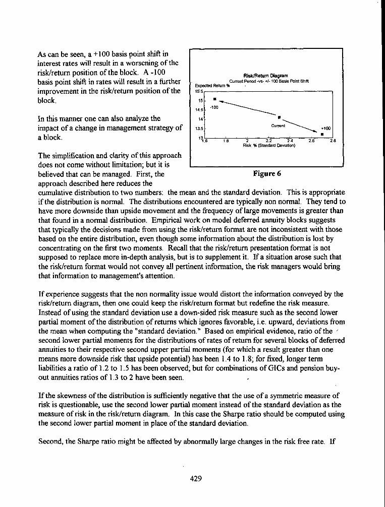
As can be seen, a +100 basis point shift in interest rates will result in a worsening of the risk/return position of the block. A -100 basis point shift in rates will result in a further improvement in the risk/return position of the block.

In this manner one can also analyze the impact of a change in management strategy-of a block.

The simplification and clarity o£this approach does not come without limitation; but it is believed that can be managed. First, the approach described here reduces the

Risk/Return Diagram CucTeOt Penod -vs- +1- 100 Basis Point Shdt

Expected Return % 155,

14.5 -1013

t,41 • n ~ 13.5 Curre

131.6 118 :2 2:2 2'4 2'.6 Risk % (Standard De',,qat~on

+100

8

Figure 6

cumulative distribution to two numbers: the mean and the standard deviation. This is appropriate if the distribution is normal. The distributions encountered are typically non normal. They tend to have more downside than upside movement and the frequency of large movements is greater than that found in a normal distribution. Empirical work on model deferred annuity blocks suggests that typically the decisions made from using the risk/return format are not inconsistent with those based on the entire distribution, even though some information about the distribution is lost by concentrating on the first two moments. Recall that the risk/return presentation format is not supposed to replace more in-depth analysis, but is to supplement it. I fa situation arose such that the risk/return format would not convey all pertinent information, the risk managers would bring that information to management's attention.

If experience suggests that the non normality issue would distort the information conveyed by the risk/return diagram, then one could keep the risk/return format but redefine the risk measure. Instead of using the standard deviation use a down-sided risk measure such as the second lower partial moment of the distribution of returns which ignores favorable, i.e. upward, deviations from the mean when computing the "staJadard deviation." Based on empirical evidence, ratio of the I second lower partial moments for the distributions of rates of return for several blocks of deferred annuities to their respective second upper partial moments (for which a result greater than one means more downside risk that upside potential) has been 1.4 to 1.8; for fixed, longer term liabilities a ratio of 1.2 to 1.5 has been observed; but for combinations of GICs and pension buy- out annuities ratios of 1.3 to 2 have been seen.

If the skewness of the distribution is sufficiently negative that the use of a symmetric measure of risk is questionable, use the second lower partial moment instead of the standard deviation as the measure of risk in the risk/return diagram. In this case the Sharpe ratio should be computed using the second lower partial moment in place of the standard deviation.

Second, the Sharpe ratio might be affected by abnormally large changes in the risk free rate. If

429

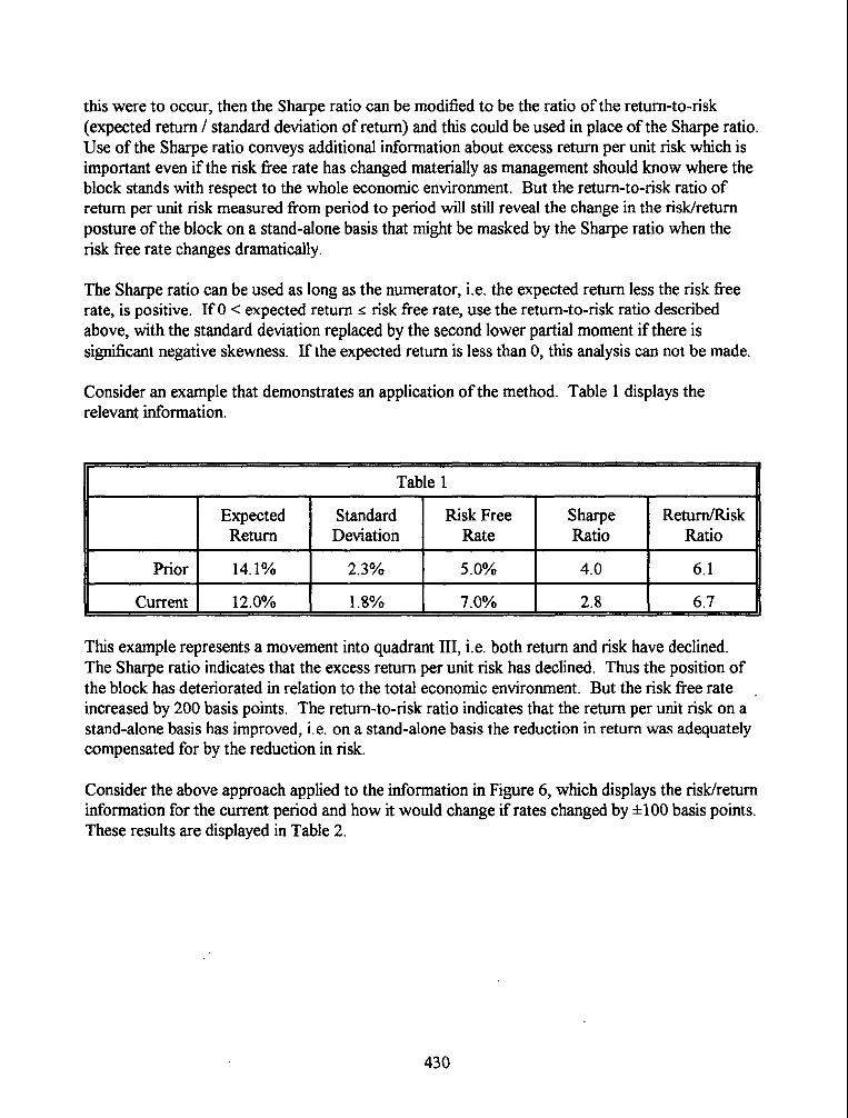
this were to occur, then the Sharpe ratio can be modified to be the ratio of the return-to-risk (expected return / standard deviation of return) and this could be used in place of the Sharpe ratio. Use of the Sharpe ratio conveys additional information about excess return per unit risk which is important even if the risk free rate has changed materially as management should know where the block stands with respect to the whole economic environment. But the return-to-risk ratio of return per unit risk measured from period to period will still reveal the change in the risk/return posture of the block on a stand-alone basis that might be masked by the Sharpe ratio when the risk free rate changes dramatically.

The Sharpe ratio can be used as long as the numerator, i.e. the expected return less the risk free rate, is positive. If0 < expected return < risk free rate, use the return-to-risk ratio described above, with the standard deviation replaced by the second lower partial moment if there is significant negative skewness. If the expected return is less than 0, this analysis can not be made.

Consider an example that demonstrates an application of the method. Table 1 displays the relevant information.

, , i i , , i i i i , , , , , ,

Table 1

Expected Standard Risk Free Sharpe Return/Risk Return Deviation Rate Ratio Ratio

Prior 14.1% 2.3% 5.0% 4.0 6.1 | | | | |

Current 12.0% 1.8% 7.0% 2.8 6.7 I I

This example represents a movement into quadrant III, i.e. both return and risk have declined. The Sharpe ratio indicates that the excess return per unit risk has declined. Thus the position of the block has deteriorated in relation to the total economic environment. But the risk free rate increased by 200 basis points. The return-to-risk ratio indicates that the return per unit risk on a stand-alone basis has improved, i.e. on a stand-alone basis the reduction in return was adequately compensated for by the reduction in risk.

Consider the above approach applied to the information in Figure 6, which displays the risk/return information for the current period and how it would change if rates changed by +100 basis points. These results are displayed in Table 2.

430

Expected Return

Table 2

Sharpe Ratio

Standard Deviation

Risk Free_ Rate

Return/Risk Ratio

2.7

-100 Shift 15.2% i 1.7°/o - 4.0o/0 6.6 8.9 | | | | |

Current 14.1% i 2.3% 5.0%- 4.0 6.1

+100 Shift ' 13.2% ,' 2.7% ' 6.0% ' 1 4.9 4.9

Note that both the Sharpe ratio and the return/risk ratio move consistently with the movements of the risk/return pairs.

Two papers by this author would be useful to those working in this area. The first ("A Generalized Profits Released Model for the Measurement of Return on Investment for Life Insurance", Society of Actuaries Transactions, Vol. XL (1988), part I, pp. 61-114) relates to the proper method for discounting distributable earnings in situations where the classical net present value algorithm fails to give economically meaningful results. The second paper ("The Value of the Firm: The Option Adjusted Value of Distributable Earnings") was part of the joint Society of Actuaries and New York University research seminar on the fair value of liabilities held in December, 1995. A copy of the second paper is available from the author upon written request sent to the author's yearbook address.

431

market value measures: duration analysis and …...want to hear about book value; they want to hear...

Documents