markov chains, lamp models and reverse-engineering
TRANSCRIPT

Markov Chains, LAMP Models and Reverse-Engineering

LAMP Models
Ravi Kumar, Maithra Raghu, Tamas Sarlos and Andrew Tomkins
[Ref: WWW 2017]

Problem setting
We consider models of sequences of outputs– Output ‘d’ can depend on earlier ‘d’ anywhere in history– Dependence on history can be learned
What if output ‘c’ is often (eventually) followed by output ‘d’?
a b b c d e b a c d cd ?

Example: Science Fiction Novels

Example: Science Fiction Novels

Example: Science Fiction Novels

Example: Science Fiction Novels
Many other examples:

Simplest approach: consider most recent element
a b b c d e b a c d cd ?Most recent letter most predictive. Following c: { a:100, b:200, c:1273, d:11 }
Can write Pr[next letter | current letter] as matrix:
First-order Markov Model MM1(W):
W =
0
BB@
0.5 0.1 0.1 0.30 0.8 0.15 0.05.06 0.13 .8 .0070.1 0.1 0.1 0.7
1
CCA
xnew = WTxold

But is this enough?
Generally, looking at more history should provide better modelsApproaches to long-range dependencies:– High-order or variable-order Markov models– Deep network sequence models– Point processes– Many others
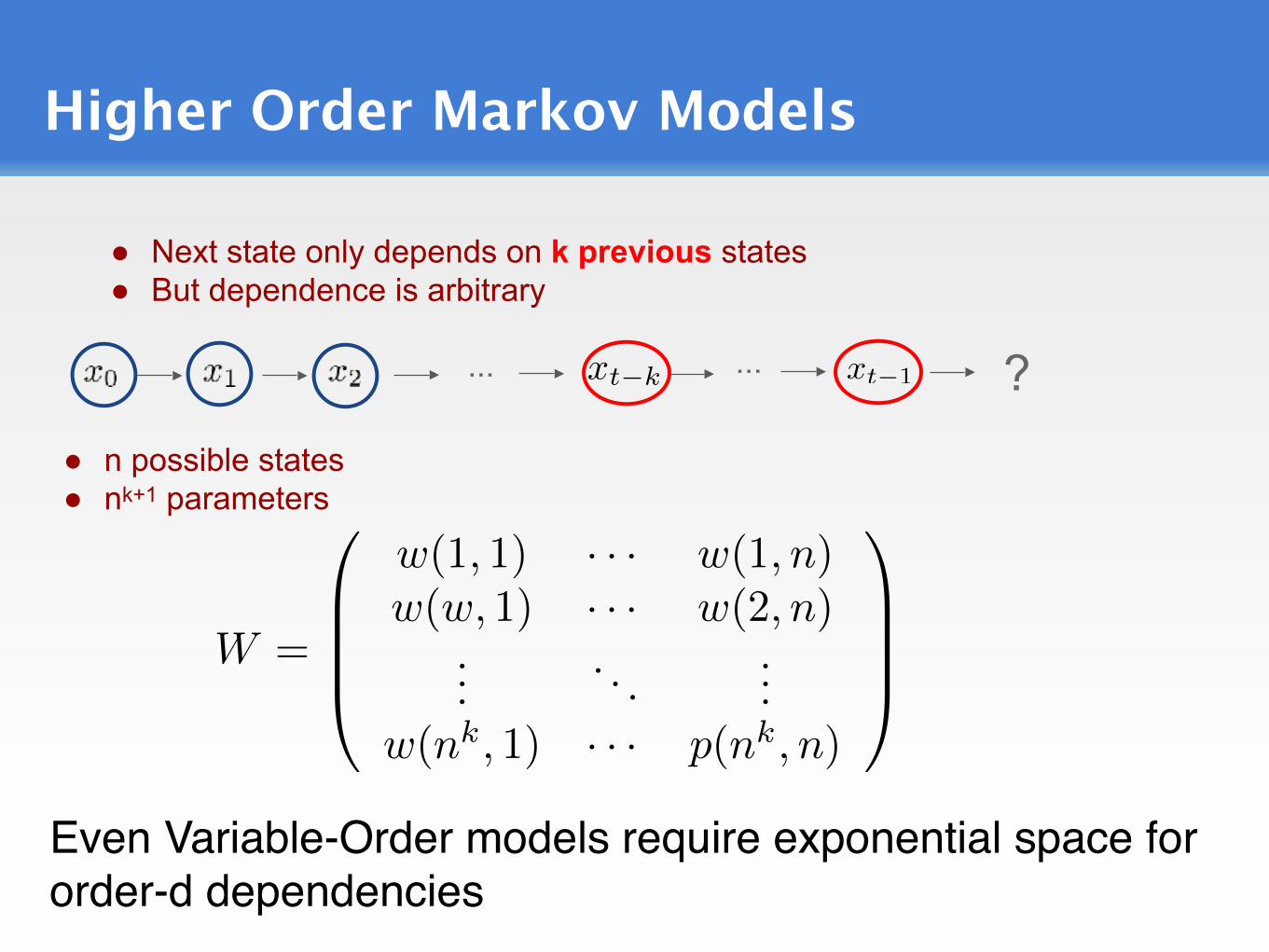
Higher Order Markov Models
● n possible states ● nk+1 parameters
● Next state only depends on k previous states ● But dependence is arbitrary
... ?...
W =
0
BBB@
w(1, 1) · · · w(1, n)w(w, 1) · · · w(2, n)
.... . .
...w(nk, 1) · · · p(nk, n)
1
CCCA
Even Variable-Order models require exponential space for order-d dependencies
xt�1xt�k

Deep Neural Network Models
Recurrent neural networks ● (Generating Sequences with RNNs, Graves, 2014)
● LSTMs (Long-Short Term Memory)
● Complex non-linear relations between previous states
Concerns ● Slow to train ● Requires lots of data

Introduction to recency weighting
Significant body of work on models of re-consumption, based on extensions of Simon’s copying model [Simon’55]:

Introduction to recency weighting
Significant body of work on models of re-consumption, based on extensions of Simon’s copying model [Simon’55]:
a b b c d e b a c d cd ?
weights w
w(1) w(2) w(3) w(4) w(5) w(6) w(7) w(8) w(9) w(10) w(11) w(12)
w(2) w(5) w(8)
Pr[d is consumed next] ~ + +

Combining Recency-Weighting with Markov
Extending the same idea to Markov models:Next state is a mixture
Joe’s Family Fun
Barn
Mortons Steak House
Shakey’s Pizza Parlor
Ruth’s Chris ??
w(1) w(2) w(3) w(4)

Linear Additive Markov Process (LAMP)
Definition of LAMPk(w, W)
● W stochastic (transition) matrix ● Vector w with k weights
Pr[Xt = xt|x0, . . . , xt�1] =kX
i=1
wiWT~1xt�i
Total parameter complexity: NNZ(W) + kMust learn both matrix W and history distribution wWe use alternating minimization — details in paper

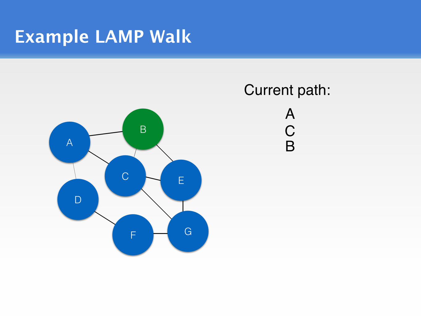
Example LAMP Walk
AB
D
F
EC
G
ACurrent path:

Example LAMP Walk
AB
D
F
EC
G
ACurrent path:
Move from

Example LAMP Walk
AB
D
F
EC
G
ACurrent path:
Move from

Example LAMP Walk
AB
D
F
EC
G
ACurrent path:
C

Example LAMP Walk
AB
D
F
EC
G
ACurrent path:
CMove from

Example LAMP Walk
AB
D
F
EC
G
ACurrent path:
CMove from
Example LAMP Walk
AB
D
F
EC
G
ACurrent path:
CB

Example LAMP Walk
AB
D
F
EC
G
ACurrent path:
CB Move from

Example LAMP Walk
AB
D
F
EC
G
ACurrent path:
CB Move from

Example LAMP Walk
AB
D
F
EC
G
ACurrent path:
CBE

Example LAMP Walk
AB
D
F
EC
G
ACurrent path:
CB
Move from
E

Example LAMP Walk
AB
D
F
EC
G
ACurrent path:
CB
Move from
E

Example LAMP Walk
AB
D
F
EC
G
ACurrent path:
CBEG

Example LAMP Walk
AB
D
F
EC
G
ACurrent path:
CB
Move from
EG

Example LAMP Walk
AB
D
F
EC
G
ACurrent path:
CB
Move from
EG

Example LAMP Walk
AB
D
F
EC
G
ACurrent path:
CBEGD

Expressivity and Evolution of LAMP
1. LAMPk(w,W) cannot be approximated by MMk-1
2. LAMPk(w,W) is a subset of MMk

Expressivity and Evolution of LAMP
1. LAMPk(w,W) cannot be approximated by MMk-1
2. LAMPk(w,W) is a subset of MMk
Time 0
State distribution of LAMP at different timesteps:
⇡0

Expressivity and Evolution of LAMP
1. LAMPk(w,W) cannot be approximated by MMk-1
2. LAMPk(w,W) is a subset of MMk
Time 0
State distribution of LAMP at different timesteps:
⇡0
Time 1
⇡0W

Expressivity and Evolution of LAMP
1. LAMPk(w,W) cannot be approximated by MMk-1
2. LAMPk(w,W) is a subset of MMk
Time 0
State distribution of LAMP at different timesteps:
⇡0
Time 1
⇡0W
Time 2
⇡0W2
⇡0W

Expressivity and Evolution of LAMP
1. LAMPk(w,W) cannot be approximated by MMk-1
2. LAMPk(w,W) is a subset of MMk
Time 0
State distribution of LAMP at different timesteps:
⇡0
Time 1
⇡0W
Time 2
⇡0W2
⇡0W
Time 3
⇡0W3
⇡0W2
⇡0W

Expressivity and Evolution of LAMP
1. LAMPk(w,W) cannot be approximated by MMk-1
2. LAMPk(w,W) is a subset of MMk
Time 0
State distribution of LAMP at different timesteps:
⇡0
Time 1
⇡0W
Time 2
⇡0W2
⇡0W
Correct random variable: exponent at time t = Evolution: pick exponent from previous k (according to w), add 1 to it.
et
[See also Wu and Gleich (arXiv)]
Time 3
⇡0W3
⇡0W2
⇡0W
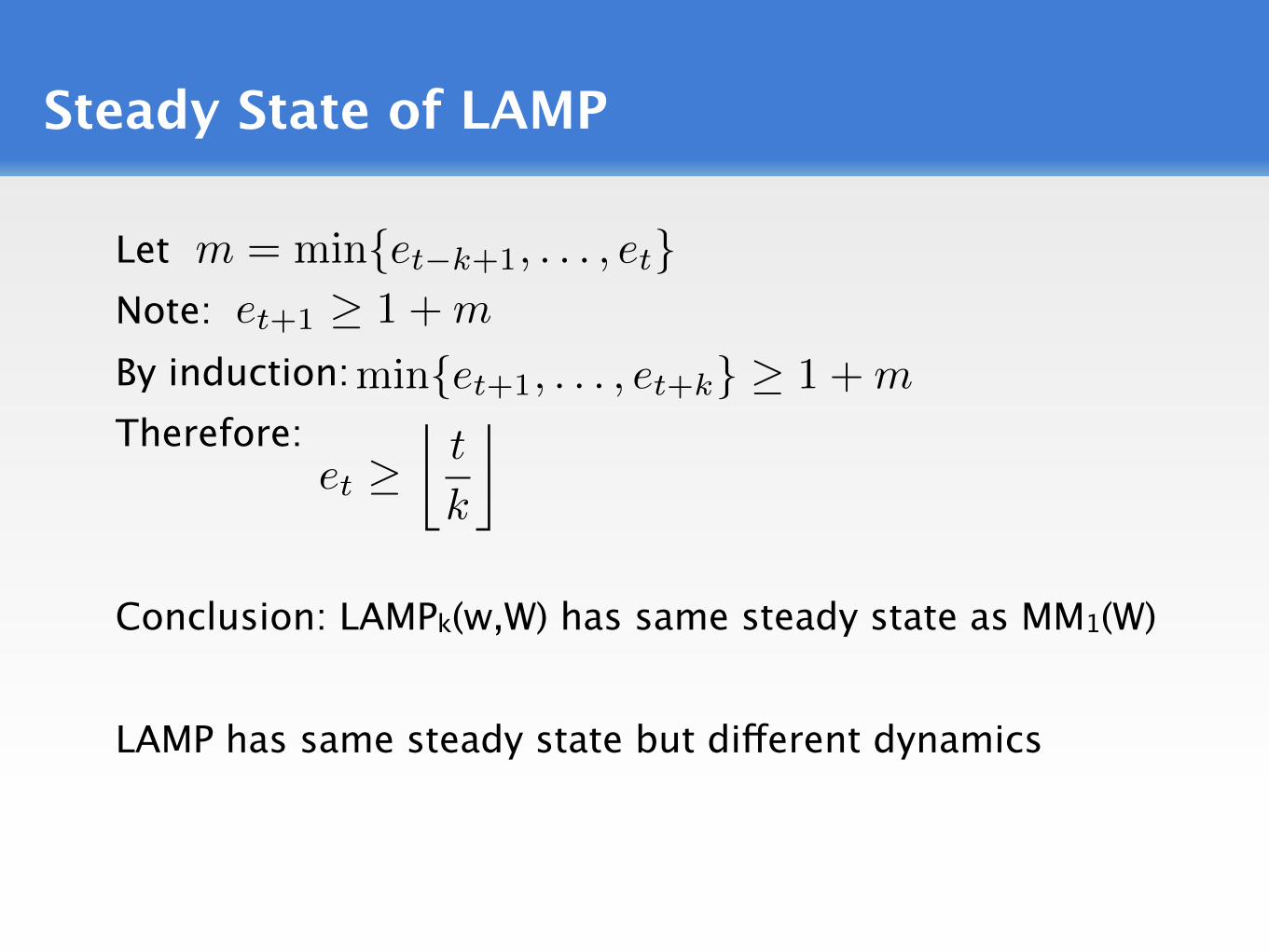
Steady State of LAMP
LetNote:By induction:Therefore:
Conclusion: LAMPk(w,W) has same steady state as MM1(W)
LAMP has same steady state but different dynamics
et+1 � 1 +m
et ��t
k
⌫
m = min{et�k+1, . . . , et}
min{et+1, . . . , et+k} � 1 +m

Exponent Processes
is a stopping time, when this sum first crosses t
But this is just a renewal process!
Theorem: By Strong Law of Large Numbers for Renewal Processes:
Look back from exponent at time t
Time: t�H(t)PI=1
Wi . . . t�W1 �W2 t�W1 t
State: ⇡0 . . . ⇡0W et�2 ⇡0W et�1 ⇡0W et
limt!1
H(t) = tE(w)

LAMP Mixing
● Can derive concentration bounds
● Gives strong statements on mixing time of LAMP, based on mixing of underlying first-order MM

Data for Evaluation
Wikispeedia

Experiments: Total Perplexity
BrightKite
Reuters
LastFM
Wikispeedia
Observations ● In general, N-grams
and Kneyser-Ney N-grams struggle to use higher order information without overfitting
● Exception is Reuters (text data) which these models have been designed to do better on

Experiments: learned weight distribution
● LAMP learns weight decay where useful (BrightKite)
● If history isn’t useful (Wikispeedia), then turns into First Order Markov Chain
BrightKite Wikispeedia

Experiments
● LAMP does better than LSTM on some datasets (e.g. BrightKite)
● Better or equal performance on other datasets (e.g. LastFM) with similar amounts of training time ○ With 20x training time, LSTM does better
● LSTM does better on text data (better at using text statistics, similar to N-grams)
Comparison with LSTMs

Reverse Engineering a Markov Chain
Ravi Kumar, Andrew Tomkins, Sergei Vassilvitskii and Erik Vee
[Ref: WSDM 2015]

Random Walks & Markov Chains
Markov Chains in Data Analysis:– Simple, yet capture a lot of interactions– Typically: compute & use the stationary distribution– Beautiful theory with great applications
Examples:– PageRank: Random surfer stationary distribution– Translation: Use language models to build phrases – ...

A Recommendation Chain

A Recommendation Chain
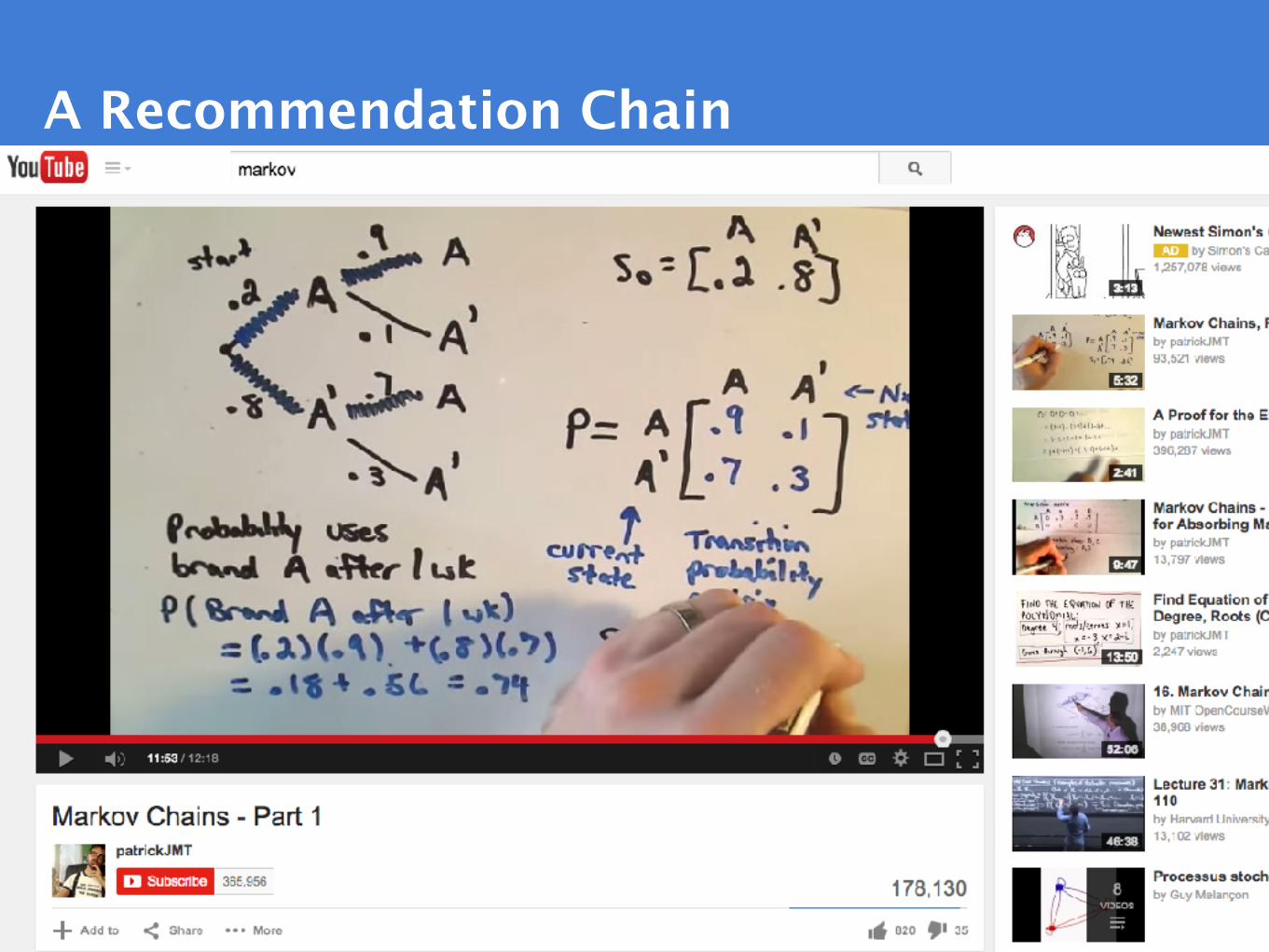
A Recommendation Chain
A Recommendation Chain

A Recommendation Chain

A Recommendation Chain
stationary distribution

A Recommendation Chain
Example:– Items: videos– Stationary Distribution: view counts
Why are some videos more popular:– Better (higher quality) videos– More frequently recommended
Today:– Disentangle these two reasons

Inverting a Markov Chain
Problem: – Given a stationary distribution, find the Markov Chain that generated
it.
Given:– Graph – Distribution
Output:– Transition Matrix that generated it
⇡
G
M

Feasibility
Feasibility:– Not always feasible
A B
⇡A = 1/3 ⇡B = 2/3
⇡

Feasibility
Feasibility:– Not always feasible
Definition:– A directed graph is consistent if there is a flow that preserves the
steady state. – Any strongly connected graph with self loops is consistent
Theorem:– For any consistent graph, there exists a Markov chain with as its
stationary distribution.
A B
⇡A = 1/3 ⇡B = 2/3
⇡

Constraints
The problem is under-constrained:– constraints– variablesn
m� n � n

Constraints
The problem is under-constrained:– constraints– variables
Approaches– [Tomlin `03]: MaxEnt objective on variables (regularization)
n
m� n � n

Constraints
The problem is under-constrained:– constraints– variables
Approaches– [Tomlin `03]: MaxEnt objective on variables (regularization) – [Today] Limit the degrees of freedom
– For each vertex let be its score. The Markov Chain is the function of the scores
– Scores express “quality” or “attractiveness”
n
vi si
m� n � n

From Scores to Transitions
Transition probability depends on:– Score of the destination– Parameter of the edge
C
B
A
D
MA!C
scwAC

Simplest Example
Weighted Random Walk:– All of the edge weights are set to 1– Transition probability proportional to the score
C
B
A
DMA!C =
sCsB + sC + sD

Simplest Example
Weighted Random Walk:– All of the edge weights are set to 1– Transition probability proportional to the score
– Transition probabilities are context dependent:
C
B
A
DMA!C =
sCsB + sC + sD
C
B
A
D
sB = 100
sC = 10
sD = 1
MA!C = 0.09

Simplest Example
Weighted Random Walk:– All of the edge weights are set to 1– Transition probability proportional to the score
– Transition probabilities are context dependent:
C
B
A
DMA!C =
sCsB + sC + sD
C
B
A
D
sB = 100
sC = 10
sD = 1
MA!C = 0.09
F
MF!C = 0.91

From Scores to Transitions
Transition probability depends on:– Score of the destination– Parameter of the edge– Call this function
Formally:
C
B
A
D
MA!C / f(sC , wAC)
MA!C =f(sC , wAC)
f(sC , wAC) + f(sB , wAB) + f(sD, wAD)
f
MA!C
scwAC

From Scores to Transitions
Transition probability depends on:– Score of the destination– Parameter of the edge– Call this function
Formally:
Sanity Check on :– Continuous in – Monotone in
C
B
A
D
MA!C / f(sC , wAC)
f
MA!C
sc
f
s
s
wAC

From Scores to Transitions
Transition probability depends on:– Score of the destination– Parameter of the edge– Call this function
Formally:
Sanity Check on :– Continuous in – Monotone in – Unbounded in :
C
B
A
D
MA!C / f(sC , wAC)
f
MA!C
sc
f
s
ss
wAC
lims!1
f(s, w) ! 1
limsc!1
MA!C = 1

Simplest Example
Weighted Random Walk:– All of the edge weights are set to 1– Transition probability proportional to the score
C
B
A
DMA!C =
sCsB + sC + sD

More Examples
Weighted Random Walk:– All of the edge weights are set to 1– Transition probability proportional to the score
Seeking Similar Content:– Edge weight: similarity between two nodes
–
C
B
A
DMA!C =
sCsB + sC + sD
MA!C / wAC · sC

More Examples
Weighted Random Walk:– All of the edge weights are set to 1– Transition probability proportional to the score
Seeking Similar Content:– Edge weight: similarity between two nodes–
Overall:– Decide whether items are popular due to high scores (attract all of the
incoming traffic) or due to location (attract a little bit from many locations)
C
B
A
DMA!C =
sCsB + sC + sD
MA!C / wAC · sC

Main Theorem
Given:– A consistent input– Monotone, continuous and unbounded function
There exists:– A unique set of scores– So that is the stationary distribution induced by – Moreover, the scores can be found in polynomial time
G,⇡
f
s1, . . . , sn⇡ f

Main Theorem
Given:– A consistent input– Monotone, continuous and unbounded function
There exists:– A unique set of scores– So that is the stationary distribution induced by – Moreover, the scores can be found in polynomial time
G,⇡
f
s1, . . . , sn⇡ f
up to scaling

Main Theorem
Given:– A consistent input– Monotone, continuous and unbounded function
There exists:– A unique set of scores– So that is the stationary distribution induced by – Moreover, the scores can be found in polynomial time
G,⇡
f
s1, . . . , sn⇡ f
up to scaling
up to (1± ✏)
Definitions
– Fix a set of scores and permutation s ⇡

Definitions
– Fix a set of scores and permutation s
C
B
A
D
E
1
1 1 1
1
1/3
2/27
4/27
1/9
1/3
⇡

Definitions
– Fix a set of scores and permutation – Let be the expected mass at
starting with using
–
svi
s
C
B
A
D
E
1
1 1 1
1
1/3
2/27
4/27
1/9
1/3⇡qi(s)
⇡

Definitions
– Fix a set of scores and permutation – Let be the expected mass at
starting with using
–
svi
s
⇡qi(s)
C
B
A
D
E
1
1 1 1
1
1/3
2/27
4/27
1/9
1/3
1/9
1/9
1/9
1/3 1/3
⇡

Definitions
– Fix a set of scores and permutation – Let be the expected mass at
starting with using
– Call a node underweight if
svi
s
⇡qi(s)
C
B
A
D
E
1
1 1 1
1
1/3
2/27
4/27
1/9
1/3
1/9
1/9
1/9
1/3 1/3
qi(s) < (1� ✏)⇡i
⇡

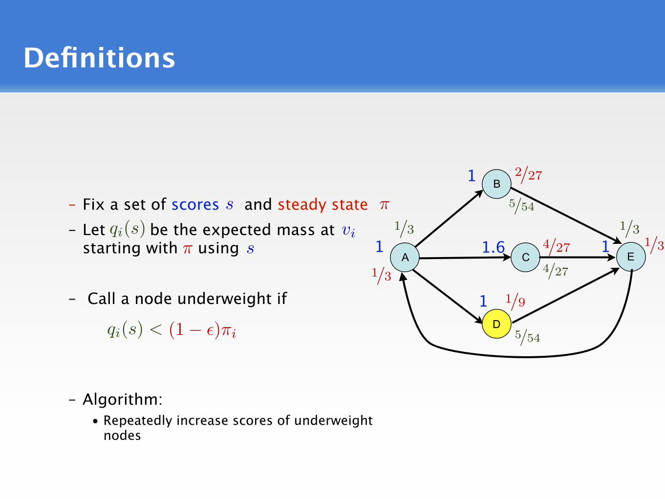
Definitions
– Fix a set of scores and steady state – Let be the expected mass at
starting with using
– Call a node underweight if
– Algorithm:• Repeatedly increase scores of underweight
nodes
svi
s
⇡qi(s)
C
B
A
D
E
1
1 1 1
1
1/3
2/27
4/27
1/9
1/3
1/9
1/9
1/9
1/3 1/3
qi(s) < (1� ✏)⇡i
⇡
Definitions
– Fix a set of scores and steady state – Let be the expected mass at
starting with using
– Call a node underweight if
– Algorithm:• Repeatedly increase scores of underweight
nodes
svi
s
⇡qi(s)
C
B
A
D
E
1
1 1.6 1
1
1/3
2/27
4/27
1/9
1/31/3 1/3
qi(s) < (1� ✏)⇡i
⇡
4/27
5/54
5/54

Definitions
– Fix a set of scores and steady state – Let be the expected mass at
starting with using – Call a node underweight if
Algorithm:– Start with – For
• For each :• If underweight:
Set• else: Set
svi
s
⇡qi(s)
qi(s) < (1� ✏)⇡i
s0i = 1/n
t = 1, . . .vi 2 V
vi
sti = st�1i
⇡
sti : qi(st�1�i , sti) = (1� ✏/2)⇡i

Definitions
Guaranteed to exist because f is monotone, continuous, unbounded & G is consistent
Note: scores never decrease
If q is ever below , it will always stay below
⇡
– Fix a set of scores and steady state – Let be the expected mass at
starting with using – Call a node underweight if
Algorithm:– Start with – For
• For each :• If underweight:
Set• else: Set
svi
s
⇡qi(s)
qi(s) < (1� ✏)⇡i
s0i = 1/n
t = 1, . . .vi 2 V
vi
sti = st�1i
⇡
sti : qi(st�1�i , sti) = (1� ✏/2)⇡i

Proof of Convergence
Key Lemma: – There is an explicit bound such that for all .M sti M i, t

Proof of Convergence
Key Lemma: – There is an explicit bound such that for all .
Proof Sketch:– Consider a set of scores that grows without bound– These scores all must be underweight (these are the only scores that
increase) – Not all scores can be underweight (sum of underweight scores below
1) – The scores growing without bound are taking all of the probability
mass from those bounded – By consistency, this demand must be met, a contradiction.
M sti M i, t
Proof of Convergence
Key Lemma: – There is an explicit bound such that for all .
Finishing the Proof:– Scores increase multiplicatively by factor of
– is bounded by
– Overall: iterations suffice.
M sti M i, t
M
✓n2W
✏pmin
◆n
O
✓n2
✏log
nW
✏pmin
◆
(1 + ✏/2)

But Does it Work...
Experimental Evaluation:– Dataset: empirical transitions – Input: Transition graph and the steady state distribution– Output: Transition probabilities– Metrics: LogLikelihood or RMSE
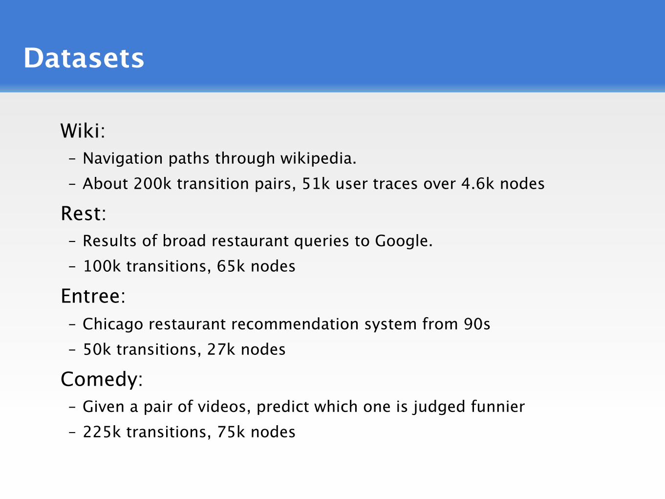
Datasets
Wiki:– Navigation paths through wikipedia. – About 200k transition pairs, 51k user traces over 4.6k nodes
Rest:– Results of broad restaurant queries to Google. – 100k transitions, 65k nodes
Entree:– Chicago restaurant recommendation system from 90s– 50k transitions, 27k nodes
Comedy:– Given a pair of videos, predict which one is judged funnier– 225k transitions, 75k nodes

Baselines
Popularity:– Transition proportionally to the steady state distribution (score = pi)
Uniform:– Uniform over out-edges
Pagerank:– Transition proportionally to the node pagerank
Temperature:– MaxEnt regularization approach
Inversion:– Our algorithm

Results
RMSE Prediction:
Popularity Uniform PageRank Tempe-rature Inversion
Wiki 1 0.65 0.83 0.65 0.57
Rest 1 1.17 1.39 1.21 0.59
Entree 1 0.69 1.01 0.56 0.42
Comedy 1 0.65 0.9 0.78 0.36

Convergence
-1
-0.95
-0.9
-0.85
-0.8
-0.75
-0.7
-0.65
0 5 10 15 20 25 30 35 0.55
0.6
0.65
0.7
0.75
0.8
0.85
0.9
0.95
1
Log li
kelih
ood
RM
SE
Iteration
Performance on WIKI
Log likelihoodRMSE

The End