Markov Renewal Programming by Linear Fractional ProgrammingAuthor(s): Bennett FoxReviewed work(s):Source: SIAM Journal on Applied Mathematics, Vol. 14, No. 6 (Nov., 1966), pp. 1418-1432Published by: Society for Industrial and Applied MathematicsStable URL: http://www.jstor.org/stable/2946249 .Accessed: 13/09/2012 22:34

Your use of the JSTOR archive indicates your acceptance of the Terms & Conditions of Use, available at .http://www.jstor.org/page/info/about/policies/terms.jsp

.JSTOR is a not-for-profit service that helps scholars, researchers, and students discover, use, and build upon a wide range ofcontent in a trusted digital archive. We use information technology and tools to increase productivity and facilitate new formsof scholarship. For more information about JSTOR, please contact support@jstor.org.

.

Society for Industrial and Applied Mathematics is collaborating with JSTOR to digitize, preserve and extendaccess to SIAM Journal on Applied Mathematics.

http://www.jstor.org

SIAM J. APPL. MATH Vol. 14, No. 6, November, 1966

Printed in U.S.A.

MARKOV RENEWAL PROGRAMMING BY LINEAR FRACTIONAL PROGRAMMING*

BENNETT FOXt

Abstract. Markov renewal programming is treated by linear fractional program- ming. Particular attention is given to the resolution of tied policies that minimize expected cost per unit time. The multichain case is handled by a decomposition ap- proach.

1. Introduction. Markov renewal programming can be described graph- ically in terms of networks consisting entirely of "branch" nodes jointed together by directed arcs with stochastic lengths.

Consider an are (i, j). It carries a vector of labels (Ltj, , ,LJ), where Lj = (pkj, ij, Ckj). Here, if of the mi alternatives available at node i

action k is taken, pkj is the probability of a transition from node i to node j, Fkj is the distribution (assumed nondegenerate at zero) of the lengtlh of are (i, j), which can be interpreted as the time to traverse the are, and C'j is the cost incurred if the transition i --j actually occurs. In general, C,, de- pends on the length t of are (i, j). An important special case is Czj(t) = ak + bkjt; here knowledge of the mean are length suffices for our purposes, except when ties occur. We assume that there are n nodes and that the setsN = {1, *,nl and M {, =I *, ml}, i E N, are finite. The nodes (under any policy) form an imbedded Markov chain assumed ergodic unless stated otherwise; i.e., the state does not depend on the path by which the node was reached and there exists a path (perhaps indirect) between any two nodes. The latter condition implies that all nodes communicate, ruling out in particular absorbing nodes. An extension to nonergodic im- bedded chains is given in ?8 and ?9.

We take as objective function expected cost per unit time; see ?2 for a precise definition. Tied policies that minimize expected cost per unit time are resolved by examining the asymptotic expected discounted cost as the discount rate a -0; details are given in ?7 and ?9. (With continuous dis- counting at rate a, a loss incurred at time x is discounted by the factor G'x.

Jewell [15] gives a precise formulation of the discouinting case and also con- siders the case a -> 0. We treat the latter case from a different viewpoint and obtain results beyond those of Jewell.)

I thank Eric Denardo for helpful comments.

2. Existence of a stationary optimal policy. If each decision, given the current node is independent of the history of previous nodes, transition

* Received by the editors November 29, 1965, and in finlal revised form April 14, 1966.

t The RAND Corporation, Santa Monica, Califorinia.

1418

MARKOV RENEWAL PROGRAMMING 1419

times, and decisions, then the correspondinig policy is called stationary. To justify the formulation of the problem that we give in the next section, we need to show that there is a stationary policy that minimizes expected cost per unit time, defined as

?(7r) = lim sup L(t; 7)

where Lj( t; 7r) is the expected cost up to time t using a policy 7r when starting at node j.

First, we need some definitions. A policy is a-optimal if it minimizes ex- pected discounted loss over an infinite horizon when continuously discount- ing at rate a. A policy is pure if it is nonrandoiiiized. We assume that ex- pected one-stage discounted loss,

QI t

JdFkij( t) Je ax dx Ck (x I t),

exists finitely for all a > 0 and all i, j, k, where Ckj(X I t) is a function of bounded variation (all t < oo ) denoting the loss up to time x during a transition i -> j of length t, when action k at state i is taken; kj(t I t) = Ckj(t). THEOREM 1. For each a > 0, a pure stationary a-optimnal policy exists.

Among the policies that minimize expected cost per unit time, there is a pure stationary one.

Proof. The first assertion follows immediately from a result of Denardo; see Theorem 5 and the discussion of Example 4 in [7]. Since there are only a finite number of pure stationary policies, it follows that there is a sequence Iail} > 0+ and a pure stationary policy a such that a is ai-optimal, i = 1, 2, * . . From the results of Jewell [15], it follows that starting from node j under a stationary policy p, the expected discounted loss Rj( a; p) has the form gp/a + 0(1) and is the Laplace-Stieltjes transform of Lj( t; p) evaluated at a; hence by standard Abelian and Tauberian theorems (see, e.g., [20, p. 181 and p. 192]), we have for any policy 7r and any starting node j,

?(7r) ? lim sup aiRj(aei; 7r) ? lim sup axRj(a i; a) = g = (a) j-iOO i-oo

showing that a minimizes expected cost per unit time. As the proof shows, with a stationary policy p, we can replace

lim sup Lj(t; p)/t by lim Lj(t; p)/t (which exists) in the definition of ?(p). For a nonergodic imbedded chain, essentially the same proof (cf. (36)) shows that the assertions of the theorem still hold, except that the expected cost per unit time then depends on the starting node.

1420 BENNETT FOX

3. Problem formulation. Denoting the stationary probability of being at node i, given that a transition has just been completed, by ri and the probability of choosing the kth alternative at node i by dik , we have ( 1) Z djkp'jprj=w, Jd k E N,

i,k

(2) Eiwi =1, (3) =k dik 1, i E N, ( 4) ri , dik >_ O, i E N, 7c E 31it With the substitutioni (cf., e.g., [10])

(5) Xik =7i dik i E N, k E Mi, (1)-(4) become

(6) ZXikPIj - X jk= 0, j - N, i,k k

(7) EXik 1; Xik _ 0 i N, ji-M, i,k

with

(8) dik = xik/ xij, iN, E c kE MI.

The denominator in (8) is rir, which is positive since the imbedded chain was assumed ergodic.

We restrict ourselves to infinite horizon problenms with one of the following objectives:

(i) minimize expected cost per transitioin; (ii) minimize expected cost per unit time.

The corresponding objective functions are, respectively, (cf. [10] and [15J)

(9) mmin XikYi , i,k

(10) mlml Z XikYi l/ E XikVik i,k i,k

where

(11) 7,t = Z pij ij, i E N, ic E Mi (expected oile-stage loss),

(12) vi' = i pVi'i, i E N, k C Mi (expected one-stage duration),

00

(13) i = f C(j(t) dFij(t), i, E N, lkE AEIi,

(14) vij = f t dFij(t), i, i E N, k C Mli.

MARKOV RENEWAL PROGRAMMING 1421

We see that (9) anid (10) are not equivalent in general; an important exception occurs when all the v'j are equal, as in an inventory problem with periodic review. On the other hand, with many maintenance problems the mean transition times between distinct pairs of nodes are different. In this situation, problem (ii) appears to be the more natural one to attack, and thus (10) is the appropriate objective functionl. We assume that 0 < vtj < 0o for alli,j, k.

The linear programming formulation of problem (i) via (6)-(7), (9), (11), and (13) is well known; see, e.g., Derman [10]. For problem (ii), we get an analogous linear fractional programming formulation via (6)-(7), (1,0), and (11)-(14).

4. Reduction to a linear program. The subject of linear fractional programming is dealt with in [4], [11], [12], [14], [16], and [18]. We shall follow Charnes and Cooper [4], although it is possible that one of the other approaches leads to a more efficient algorithm.' As a first step, note that the denominator in (10) is positive and the feasible solution set is non- empty and bounded. Hence, for problem (ii) we obtain the following equiva- lent linear program:

( 15 ) mmin Z Yik-N' ,k

subject to

(16) ZYikP}U ZYjk 0, J CS, i,k k

(17) Y t=0, i,k

(18) E YikVi= 1, i,k

(19) YikitB 0x iEN, kEMi, with

(20) Xik = Yik/t,

and S = { 1, ... , n- 1}. We have dropped the (redundant) constraint cor- responding to the nth of the relations (6). It can be shown [4] that t > 0; in fact, (17) is redundant. In view of (8) and (20),

(21) dik = yik/Z yi iG N, kIE Mi. i

I It has recently been shown that the approaches in [4] and [181 are equivalent. See [221.

1422 BENNETT FOX

The dual program is

(22) max g

subject to n-I

(23)~~~~~~~~~~ i Cr SIkxM (23)~~~~~~~~~~~~~~~~~~~~~~~~~~~~~~~~~~~~~~~~~~~~~~v v- 2., vjp8b + z + gv <wYX iCS,kC x j=1

n-1 (24) - Vjpkj + z + gVkc < YnI k CM

(25) -z < 0

with no sign restrictions on g or the vu . Since it is clearly optimal to take z = 0, (23)-(25) reduce to

(26) g < (_y.k+ Zvijpk i u)/ k iCY k CE Mi7

where we set Vn = 0. In this form, the dual program has a marked re- semblance to Jewell's policy iteration algorithm [15]. If all the vkj are equal, then Jewell's algorithm reduces to Howard's algorithm [13]; in this case, the relation of the dual linear program to the policy iteration routine is well known; see, e.g., [2], [9], and [19]. Jewell's algorithm amounts to applying the dual simplex method (see, e.g., [5]) to the dual program, except that multiple substitutions are allowed. The dual simplex method can be abbrevi- ated for this application by always working with a reduced basis in which no slack variables appear.

We remark that in the case of discounting, d'Epenoux [5] gives a linear programming formulation, later generalized by Denardo [7], that can be adapted to the present case. Denardo [7] gives a policy improvemen-t routine that contains the one in Jewel [15] as a special case. For the discounting case, it is not assumed that the imbedded chain is ergodic.

5. Reduction to a pure strategy. Note that the primal program has n + I constraints. Hence, there is a solution with at most n + 1 variables positive, one of which must be t, [4]. By (5) and (20) this implies that there is a solution with at most n of the dik positive. By (3), this implies that, for each i, there is exactly one k, say k(i), such that dik(i) = 1 and dik = 0, k # k(i); a proof by contradiction is immediate. Thus, we have proved:

THEOREM 2. The simplex method applied to the primal program produces a pure optimal strategy.

COROLLARY. In any basic solution, yik > 0 if and only if dik = 1. 2 It follows that the primal is nondegenerate. Hence cycling cannot occur.

MARKOV RENEWAL PROGRAMMING 1423

In practice, we may be able to guess a fairly good pure strategy. Setting those yik = 0 for which dik = 0, the remaining Yik and t can be obtained using (16)-(18). Note that the set of positive yik and t form a basic feasible solution to the primal program that can be used to initiate "phase two" of the simplex method. The primal is easier than the dual to solve initially because the former has far fewer contraints. For large scale problems, de- composition should be considered; see [5] and [21]. Whether or not our approach leads to a more efficient computational scheme than the policy iteration approach ( [13], [15] ) is an open question. Note that policy iteration in geineral requires block pivoting [5] whereas for the simplex method ordi- nary pivoting suffices.

6. Sensitivity analysis. For sensitivity analysis, the relations (26) should be quite useful. Relatively simple calculations show how a marginal change in a pij, ij , or yk affects the value of max g, which equals the minimum expected cost per unit time by the fundamental duality theorem; see, e.g., [5]. To perform the calculations, we may obtain v1, , vn_1 from

( 27 ) vi - E Vjpkji) = y -q gvk(i) ipN, j

with v- = 0 and k(i) an optimal action at node i. In practice, most linear programming codes have a provision for outputting the simplex multipliers; thus, v1, * , vn-1 can be obtained as a byproduct of the primal solution.

7. Ties and near-optimal policies. Provided that the (mild) conditions (47) of Appendix 1 hold, Jewell [15] has shown that, when continuously discounting at rate a, the expected present value Ri( a) of the overall loss starting in state i is, with a approaching zero (and following a fixed policy):

(28) J?i(a) = g/a + wi + o(l), i C N,

where wi, the bias term for state i, can be computed from the formulas in Appendix 1. Only wn need be computed using these formulas, since (cf. [15]) we have:

LEMMA 1.

(29) Wi = Wn + vi i E S.

Proof. n

Ri(a) = yi(a) + , pij5ij(a)Rj(a), j=l

where -yi( a) is the expected discounted one-stage loss and bij( a) is the Laplace-Stieltjes transform of Fij evaluated at a. For a > 0 and i, j G N,

1424 BENNETT FOX

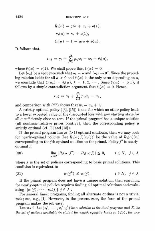
Ri(a) = ga/ + wi + o(l),

'Yi(a) = yi + o(l),

bij(a) = 1 - avij + o(a).

It follows that n

vig = Yi + Zp ijWj - Wi + Oi(a), j=1

where Oi(a) = o(1). We shall prove that Oi(a) = 0. Let {ak} be a sequence such that al = a and Iak} - 0+. Since the preced-

ing relation holds for all a > 0 and Oi( a) is the only term depending on a, we conclude that Oi(ak) = Oi(a), k = 1, 2, * . . Since O*(a) = o(1), it follows by a simple contradiction argument that 6j(a) = 0. Hence

n

vi g = 'Yi + Z piWj - X

and comparison with (27) shows that wi = Wn + Vi . A strictly optimal policy ([3], [15]) is one for which no other policy leads

to a lower expected value of the discounted loss with any starting state for all a sufficiently close to zero. If the primal program has a unique solutiorl (all nonbasic relative prices positive), then the corresponding policy is strictly optimal (cf. [3] and [15]).

If the primal program has m (> 1) optimal solutions, then we lmay look for nearly-optimal policies. Let Ri(a; j)[wi(j)] be the value of Ri(a)[wi] correspondinig to the jth optimal solution to the primal. Policy j* is niearly- optimal if

(30) lim [Ri(a; j*) -Ri(a;j)] < 0, i C N, j C J, a-o+

where J is the set of policies corresponding to basic primal solutions. This condition is equivalent to

(31) wi(j*) _ wi(j), i C N, j C J.

If the primal program does not have a unique solution, then searching for nearly-optimal policies requires finding all optimal solutions and evalu- ating { [wl(j), e * * , Wn(j)]:j J} E

For general linear programs, finding all alternate optima is not a trivial task; see, e.g., [1]. However, in the present case, the form of the primal program makes the job easy.

LEMMA 2. Let (v1o, - - * X Vn?; g0) be a solution to the dual program and Ki be the set of actions available in state i for which equality holds in (26); for any

MARKOV RENEWAL PROGRAMMITNG 1425

element of the Cartesian product K = X iENKi the same values (v10 * * vn0; 9 0) are obtained from (27).

Proof. The result is an imimediate conise(uence of the definition of K. Noting that a policy can be described in terms of a vector (a1, a. ),

where ai is the action taken in state i, we have: THEOREm 3. The set of (pure, stationary) policies that minimize expected

cost per unit time is K; i.e., J = K. Proof. All alternate optima lie on the face of the constraint set that is on

the hyperplane

EYikY i = g . i,k

A vertex of the constraint set is on this face if and only if all elements of the corresponding basis have relative price zero with respect to the mul- tipliers (vl0, ... * vn-1). Strict inequality holds in (26) on the complement of K, implyinig that the relative prices in the primal on the complement of K are positive for any primal basis corresponding to an element of K. By the lemma, the relative prices on K are zero. Combining these facts shows that K is the set of primal solutions.

Another result that follows easily from the lemma is the following. THEOREM 4. A nearly-optim7al policy exists. Proof. By Lemma 2 and Theorem 3, the vector of relative values of the

bias terms in (28) is the same for all j E J. Hence, it suffices to compare the bias terms Wn(j) for j E J; a minimum is attained for some j* since J is a finite set.

It is not known whether a strictly optimal policy exists in general. For the discrete case, Blackwell [3] has shown that such a policy does exist, but his (nonconstructive) method of proof does not extenid to the con- tinuous discounting case. It is clear that a strictly optimal policy, if it exists, must also be nearly-optimal. Hence, if there is a unique nearly- optimal policy, no better policy exists; in fact, it is easily shown that it is strictly optimal. In case of multiple nearly-optimal policies, there is ap- parently no general way to discover which (if any) are strictly optimal.

8. Nonergodic imbedded chain. I. For a fixed policy, if the imbedded chain is not ergodic, there are in ergodic subehains plus a set T consisting of t transient states. We assume that the ergodic subehains are the same for all policies. (De Cani [6], following Howard [13], heuristically derives a general algorithm, where one must keep track of the ergodic subehains at each step.)3 For each ergodic subehain, we solve a primal program of the

3There is a lacuna in Howard's proof that his algorithm converges to an optimal policy. His argument leaves open the possibility of cycling through a fixed periodic sequence of policies producing the same set of transient states, with the actions in

1426 BENNETT FOX

type already considered. Call the minimal loss rate for the ith subehain gi and the corresponding set of states Ei . In this section, if there is more than one policy that minimizes expected cost per unit time, the tied policies are not resolved. That problem is dealt with in the next section.

To avoid trivialities, we assume that t > 0. With expected loss per unit time as objective function, the losses and transition times in the transient states are immaterial; hence, we set these losses equal to zero and the transition times equal to one. To the original set of transient states, we adjoin n + 1 additional states so , si, ... , Sm with the loss in si equal to gi , i > 0. The loss is zero in the absorbing state so . Computing the transition prob- abilities { qkj} for the t + m + 1 state chain in the obvious manner, we have

fE pi*j, i E Ty,j= si,i 1>* ..ml |j'GE Bi

(32) q., j = )P1, ,j C

1, i = Si, j = se , it 0, 1, * m,

0, otherwise.

Using either the linear fractional program of Derman [10] or the policy improvement algorithm of Blackwell [3], the best actions to take in the transient states can now be found. This can be viewed as the master prob- lem in a decomposition scheme with m independent subproblems.

9. Nonergodic imbedded chain. II. The preceding formulation of the multichain case is satisfactory, provided that there is a unique policy that minimizes expected cost per unit time. We shall give an algorithm that re- solves ties. In the sequel, gj [wj] is the loss rate (bias term) for state j.

First, we have (for a fixed policy) for all i E N and all a > 0,

(33) Ri(a) = yi(a) + Ai(a) + BR(a),

where

(34) Ai(a) = E piii(a)Rj(a), jET

(35) Bi(a) = E pij[gJa - vijgj + wi] + o(1), j T

the last equation following from Jewell's result (28) for ergodic chains. We number the states so that the first t states are transient.

Let g = (g , , gt)', w - (w , , we), x = (xi , . , xt), y = (Yi , * * *, yt), R(a) = (Ri(a), R, t(a))', and e = (1, ... , 1)', the ergodic states remaining unchanged. It turns out that cycling cannot occur. Elsewhere, a proof of this fact and a linear programming formulation for the general multichain case will be presented (joint work with E. V. Denardo).

MARKOV RENEWAL PROGRAMMING 1427

the prime denioting transpose. With Q the submatrix of { pij} correspondiing to the transient states, we have:

THEOREM 5.

(36) R(a) = g/a + w + eo(l),

(37) g = (I -Q)-x, (38) w- (I-Q)-ly,

where

(39) xi= Epijgj i ET, jf T

n

(40) Yi= i- E ip fjgj + E pijwj, i e T. j=t ji T

Proof. To show (36), suppose that f( a) is an additional term appearing in the asymptotic expansion of R (a) but that f(a) $ eo(1). Without loss of generality, we may assume that f(a) does not contain a linear combina- tion of the preceding terms. Since (33) is satisfied for all a > 0, (I - Q) *f(a) = 0. It is well known that (I - Q) is nonsingular (see, e.g., [17]). Hence f(a) = 0.

Since (33) is satisfied for all a > 0, a simple contradiction argument shows that the terms in a-' cancel. This proves (37). The proof of (38) is similar.

We define a policy o- to be nearly [strictly] optimal if for every policy p the corresponding matrix {gi - gi- , wi - wi} has every row lexicographically [5] nonnegative [positive]; e.g., o- is nearly optimal if and only if for every policy p and all i E N, giP > gia and gip = giq imply wip > wi,. We shall show how to find the nearly optimal policie (which exist).

Let a policy p be decomposed into (4, 6), where 4 [6] is the set of decisions corresponding to the transient [ergodic] states. With Q(O) the submatrix of pij(p) } corresponding to the transient states and for i f T denoting the

lexicographically minimal pair (gi, wi) by (gi0, wi?), we define a pair of operators on t-dimensional Euclidean space; let

(41) H1(g; 4) = Q(O)g + t('),

(42) H2(w; 4, g) = Q(4)w + O(4),

where 4 E MT = XiETMi, and for i E T,

(43) P)I E = Zp.(i)g 0 if T

(P (i) (i) () V () 0_ (44) [o(4,)] i = - Z ptJ !Xgj- ,pX [Vijgw - ]. jET j( T

It is easily checked that both H1 and H2 satisfy the conditions of Theorem 4

1428 BENNETT FOX

in [7]; e.g., with the metric d(x, y) = maxiET xi- yi 1, H1N and H2N are contraction mappings for some N since QN(0) ->0 for all 4 and MT is a fi- nite set. In fact, it can be shown that there is a c < 1 such that Qt(0))e < ce.) Hence, the operator

(45) A1(g) =min Hd(g; ) OEM7T

has a unique fixed point, say go. Similarly, with Go the (nonempty) set of minimizers of Hj(g0; k),

(46) A2(w) = minH2(W i; 9 4 ) OE GO

has a unique fixed point, say w?. Let Wo be the set of minimizers of H2(w0; X, go). From the preceding remarks, we have:

THEOREM 6. Let If be the components of a nearly optimal policy correspondZ- ing to the ergodic states. If a' - W?, the policy (o-', I") is nearly optimnal.

The first step is to find (gP, ' 0) for i i T. With m ergodic subehains, this requires solving m subproblems of the type already considered.5 Two appli- cationis of the policy improvement routine in [7] then yield the set of nearly optimal policies in a finite number of steps.6' Using A1 in the first application G'1 is found. Next, using A2 , we get W?. Alternatively, Go can be found using the results of Derman or Blackwell, as outlined in the preceding section.

It can be shown [7] that Go = X iEOTG and Wo = X TWI, where GP = {+(i): 4 E Go} anid WV = {4(i): 4 E W?}. This result complements Theorem 3.

To see that a nearly optimal policy exists in the general case where the ergodic subehains depend on the policy, it suffices to note that there is a pure stationary policy a- and a sequence {ai} ->O+ such that a- is ai-optimal, i 1 2, I . , which implies that Igo wo} is lexicographically minimal.

Appendix 1. Computation of the bias terms. Initially, we assume that we have a fixed policy with an ergodic imbedded chain and drop the super-

4If there is a single ergodic subehain and we seek the optimal actions for the tran- sient states, finding (gli, v,0) for i { T su-ffices by Lemma 1, Lemma 2, and Theorem 3. In this case, the minimal loss rate for every state is the same; we need to calculate the bias terms only to break ties (if any) in the ergodic states. With more than one ergodic subehain, the relative values of the bias terms within each ergodic subehain no longer suffice to break ties in the transient states.

5 If the original problem has a subehain structure that depends onl the policy, but all policies (fouind usinig a general mutltichain algorithm) that produce miinimal loss rates for every starting states have the same subehain structure, ties canl be broken in like manlner.

6 As an alternative to policy improvement, [7] contains a mathematical program- ming formulation, which in our case reduces to a linear progra,m.

MARKOV RENEWrAL PROGRAMMING 1429

script k. Under the conditionis

(i) j = t2 dFij(t) < oo i, E N, (47) n G t

(ii) -a:, < Xj 5 Pik f dFjk(t)f x dx Cjk(X t) < 0 k=l O

Jewell [15] lhas shown that (28) holds with the bias term given by

(48) wi = + ? [A2(/ )2 ij xj (2) Miii

where, with Pi(2) defined analogously to vi, n

(49) ,u;; = (=/7ri) I Pk,

n na n ('50) 42 = (17lrj) (2) + 2 ir Pink inj

i=l __m=1 i=1

n

(51) Aii- E Pik Ikj + Viz k=1 k#j

The expression for Xj looks different in form from the corresponding expres- sion in [15], but integration by parts shows that they are equivalent.

Let {Yik(i), t: i C N} be the solution to the primal program. Then, (48) aind (49) become, respectively,

n (52) JJ = [l/Y]k(i x Yik(i) Vi,

n ~~n n (53) AU = [l/zIjk(j)j Yik(i)V' + 2EE Yki r.

Having founid explicit expressions for ljj and g42), it remains to solve the systenm (51), which reduces to n relationis of the form

(54) BjAj

where

Iii = (Ali * A*nj)',

V = (PI j, . . ., Vn)17

with Bj an n X n matrix obtained by replacing column j of the matrix f pij} of transition probabilities by zeros and subtracting the result from the identity matrix. Using a proof similar to that of an analogous theorem in

1430 BENNETT FOX

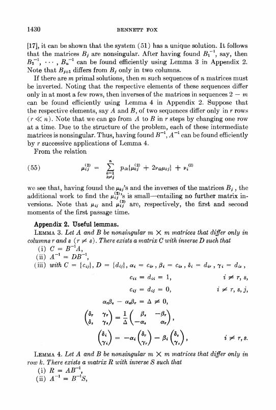
[17], it can be shown that the system (51) has a unique solution. It follows that the matrices Bj are nonsingular. After having found Bi-', say, then B271 ... , B,J1 can be found efficiently using Lemma 3 in Appendix 2. Note that Bj+i differs from Bj only in two columns.

If there are m primal solutions, then m such sequences of n matrices must be inverted. Noting that the respective elements of these sequences differ only in at most a few rows, then inverses of the matrices in sequences 2 - m can be founid efficiently using Lemma 4 in Appendix 2. Suppose that the respective elements, say A and B, of two sequences differ only in r rows (r << n). Note that we can go from A to B in r steps by changing one row at a time. Due to the structure of the problem, each of these intermediate matrices is nonsingular. Thus, having found B-1, A-' can be found efficiently by r successive applications of Lemma 4.

From the relation n

(2) A2 Vi2 (55) =j Z pPik 4k + 2Yikjk } ? (i

kHj

we see that, having found theM,ik's and the inverses of the matrices Bj, the additional work to find the Au 's is small-entailing no further matrix in- versions. Note that ,ij and ju() are, respectively, the first and second moments of the first passage time.

Appendix 2. Useful lemmas. LEMMA 3. Let A and B be nonsingular m X m matrices that differ only in

columns r and s (r # s). There exists a matrix C with inverse D such that (i) C= B-=A, (ii) A-' = DB-= (iii) with C = {cj}, D = IdijJ, xai = Cir, /3i = ci,, b, = dir , yi = ds

Cii = dii = 1, i $ r, s,

cij =d ij = O, r, s, j,

aOrf3s - a.813. = A , ?

{at YrA I As _# r

(7i - (7T) - ' ) is ar, S.

LEMMA 4. Let A and B be nonsingular m X m matrices that differ only in row k. There exists a matrix R with inverse S such that

(i) R =AB- (ii) A-1 =B-s

MARKOV RENEWAL PROGRAMMING 1431

(iii) with R = {rij} and S = fsij},

ri= = 1, i 5 k,

rij = sij = 0, i # k, j,

rkk $? 0,

Skk = l /rkk X

Skj = -rkj/rkk , j k 1.

The straightforward proofs are omitted.

REFERENCES [1] M. L. BALINSKI, An algorithm for finding all vertices of convex polyhedral sets,

this Journal, 9 (1961), pp. 72-88. [2] , On solving discrete stochastic decision problems, Naval Supply System

Research Study 2, Mathematica, Princeton, 1961. [3] D. BLACKWELL, Discrete dynamic programming, Ann. Math. Statist., 33 (1962),

pp. 719-726. [4] A. CHARNES AND W. W. COOPER, Programming with linear fractional func-

tionals, Naval Res. Logist. Quart., 9 (1962), pp. 181-186. [5] G. B. DANTZIG, Linear Programming and Extensions, Princeton University

Press, Princeton, 1963. [61 J. S. DE CANI, A dynamic programming algorithm for embedded Markov chains

when the planning horizon is at infinity, Management Sci., 10 (1964), pp. 716-733.

[7] E. V. DENARDO, Contraction mappings in the theory underlying dynamic program- ming, SIAM Rev., to appear.

[81 F. D'fPENOUX, Sur un probleme de production et de stockage dans l'aleatoire, Rev. Franqaise Rech. Oper., 14 (1960), pp. 3-16.

[9] GUY DE GHELLINCK, Les problemes de dgcisions s6quentielles, Cahiers Ceentre Ptudes Rech. Oper., 2 (1960), pp. 161-179.

[10] C. DERMAN, On sequential decisions and Markov chains, Management Sci., 9 (1962), pp. 16-24.

[111 W. DINKELBACH, Die Maximierung eines Quotienten zweier linearer Functionen unter linearen Nebenbedingungen, Z. Wahrscheinlichkeitstheorie, 1 (1962), pp. 141-145.

[12] W. S. DORN, Linear fractional programming, IBM Research Report RC 830, 1962.

[13] R. A. HOWARD, Dynamic proqramming and Markov processes, John Wiley, New York, 1963.

[14] J. R. ISBELL AND W. H. MARLOW, Attrition games, Naval Res. Logist. Quart., 3 (1965), pp. 71-93.

[15] W. S. JEWELL, Markov-renewal programming. I and II, Operations Res., 11 (1963), pp. 938-971.

[16] H. C. JOKSCH, Programming with linear fractional objective functions, Naval Res. Logist. Quart., 11 (1964), pp. 197-204.

[17] J. G. KEMENY AND J. L. SNELL, Finite Markov Chains, Van Nostrand, Princeton, 1960.

1432 BENNETT FOX

[181 B. MARTOS, Hyperbolic programming, Naval Res. Logist. Quiart., 11 (1964), pp. 135-156. (Transl. from Magyr Tud. Akad. Mat. Kutat6 Tnt. K6zl., 5 (1960), pp. 383-406.)

[191 H. WEDEKIND, Primal- und Dual-Algorithmen zur Optimierung von Markov- Prozessen, Unternehmensforschung, 8 (1964), pp. 128-135.

[20] D. V. WIDDER, The Laplace Transform, Princeton ITniversity Press, Prince- ton, 1946.

[21] P. WOLFE AND G. B. DANTZIG, Linear programming in a Mlarkov chain, Opera- tions Res., 10 (1962), pp. 702-710.

[22] H. W.XGNER AND J. S. C. YUAN, Algorithmic equivalence in linear fractional pro- gramming, Tech. Rep. 17, Graduate School of Business, Stanford Uni- versity, Stanford, 1966.