6.082 Fall 2006 1 of 28 Lab #5

Massachusetts Institute of Technology Dept. of Electrical Engineering and Computer Science

Fall Semester, 2006 6.082 Introduction to EECS 2

Lab #5: Digital Modulation

Goal:.................................................................................................................................... 2 Instructions:......................................................................................................................... 2 PreLab:................................................................................................................................ 3

A. Sigma-Delta Encoding ............................................................................................... 4 B. Upsampling and Interpolation for Data Transmission ............................................... 6 C. Eye Diagrams and Constellation Diagrams ............................................................. 10

1. Eye Diagrams........................................................................................................ 11 2. Constellation Diagrams......................................................................................... 15

Lab Exercises (2pm – 5pm, Wed., October 18, 2006):..................................................... 19 A. Viewing the Received Spectrum.............................................................................. 19 B. “Building” the Analog Receiver .............................................................................. 21 C. “Building” the Digital Receiver ............................................................................... 23

Check-off for Lab 5 .......................................................................................................... 27 Postlab............................................................................................................................... 28

6.082 Fall 2006 2 of 28 Lab #5

Goal: Basic understanding of digital modulation concepts and associated characterization methods (such as eye diagrams and constellation diagrams). The use of Sigma-Delta techniques to achieve a 2-bit/symbol data stream from a 16-bit input data stream will also be included in the exercises. Instructions:

1. Download the Prelab5 files from the 6.082 website and place them at an appropriate location on a computer with Matlab (either an Athena terminal or your own computer). In this document, we will refer to these files being in directory ~/Prelab5, though you can place them wherever you wish.

2. Be sure to complete the Prelab in its entirety before lab on Wednesday. You will need the knowledge gained from the Prelab to do the Lab exercises.

3. Complete the activities for Wednesday’s lab (see below) and get checked off by one of the TAs before leaving. You may work either in pairs or by yourself while in lab.

4. Complete the Postlab and turn in on Friday, Oct 20.

6.082 Fall 2006 3 of 28 Lab #5

PreLab: Lab 5 will focus on receiving digitally modulated data sent wirelessly from a separate transmitter to your USRP board, and then recovering the information by using various Matlab functions. In this Prelab, we will examine several operations that are used to encode, examine, and retrieve the information in digital form. As such, you will gain insight on how the transmitter works, and will also understand some of the basic tools and methods required for properly extracting the received information within lab. This information will, in turn, provide you with the basic insight and tools you need to set up a receiver in the lab itself. The figure below illustrates the overall communication link that we will be exploring. Let us first focus on the time-domain view shown in the figure. A high resolution input (corresponding to music) is first sent into a Sigma-Delta modulator in order to encode the signal as a 2-bit digital sequence. That signal is then sent into a transmitter which modulates it to a 457 MHz carrier and then radiates it out of an antenna. The receiver demodulates the signal recovered from its antenna, and then ideally reproduces the 2-bit/symbol digital sequence sent by the transmitter. To recover the music, the 2-bit/symbol digital sequence is sent through a lowpass filter.

Time Domain

Frequency Domain

Σ−∆

Digital Σ−∆Modulator

16-bit 2-bit

Input Filtered

Output

Digital Input

Spectrum

Filtered Output

Spectrum

Quantization

Noise

Receive

(Ideal communication link)

Transmit

As represented by the frequency domain view in the above figure, the digital communication link ideally passes the digital 2-bit sequence from the transmitter input to receiver output without modification. However, even in this ideal scenario, we note that we do not obtain a perfect reproduction of the original music waveform. This issue is seen in the fact that the Sigma-Delta encoding process adds quantization noise to the signal. If we had very high bandwidth in the link, we could make the over-sampling ratio of the Sigma-Delta encoding high as well so that the quantization noise could be reduced to insignificant levels after filtering without disturbing the original signal. Unfortunately, the bandwidth offered by the USRP transmit/receive system will be too small to afford

6.082 Fall 2006 4 of 28 Lab #5

such a high over-sampling ratio. It will therefore be important to understand the tradeoffs involved in using the Sigma-Delta encoding process for this lab. Note that Sigma-Delta encoding is typically only a first step in creating a digital signal from a corresponding analog signal. In later labs, we will explore additional steps which are taken to compress the digital signals with little perceptual degradation. Such compression allows more signals to be packed into a given amount of spectrum, and therefore is of high importance in achieving practical wireless systems.

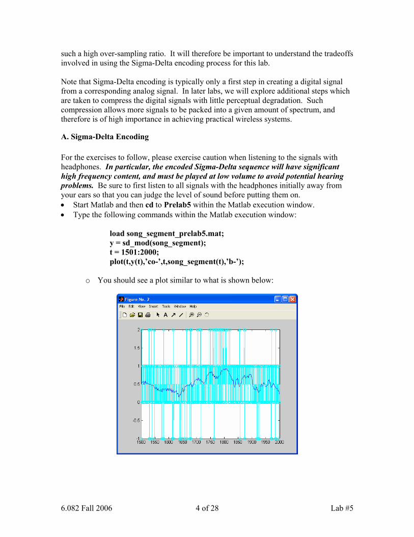
A. Sigma-Delta Encoding For the exercises to follow, please exercise caution when listening to the signals with headphones. In particular, the encoded Sigma-Delta sequence will have significant high frequency content, and must be played at low volume to avoid potential hearing problems. Be sure to first listen to all signals with the headphones initially away from your ears so that you can judge the level of sound before putting them on. • Start Matlab and then cd to Prelab5 within the Matlab execution window. • Type the following commands within the Matlab execution window:

load song_segment_prelab5.mat; y = sd_mod(song_segment); t = 1501:2000; plot(t,y(t),’co-’,t,song_segment(t),’b-’);

o You should see a plot similar to what is shown below:

6.082 Fall 2006 5 of 28 Lab #5

o The above waveforms indicate how the digital encoding of the 2-bit sequence generated by the Sigma-Delta modulator compares to the original music waveform.

• To get a better sense of the properties of the 2-bit Sigma-Delta generated sequence, let us now examine its frequency domain content by typing the following in Matlab:

f = (0:length(y)-1)*250e3/3/length(y) - 250e3/6; plot(f,abs(fftshift(fft(y-mean(y)))))

o You should see a plot similar to what is shown below. The energy content at low frequencies corresponds to the original music waveform, and the energy content at higher frequencies corresponds to the `shaped’ quantization noise created by the Sigma-Delta encoding process. Notice from the Matlab code above that the sample rate is Fs = 250kHz/3 (i.e., 83.3 kHz).

• We now seek to recover the original music signal by lowpass filtering the 2-bit Sigma-Delta output sequence. We will do so with three different filter bandwidths in order to understand key tradeoffs in this operation. As such, type the following commands in Matlab:

lowpass1 = fir1(100,0.08); % bandwidth of 0.08*Fs/2 lowpass2 = fir1(100,0.12); % bandwidth of 0.12*Fs/2 lowpass3 = fir1(100,0.15); % bandwidth of 0.15*Fs/2

y_filt1 = filter(lowpass1,1,y); y_filt2 = filter(lowpass2,1,y); y_filt3 = filter(lowpass3,1,y);

6.082 Fall 2006 6 of 28 Lab #5

• Now play each of the above filtered waveforms on the headphones one by one and compare the sound of each. Be sure to adjust the computer headphone volume properly before placing the headphones directly on your ears. Be especially careful if you want to listen to the unfiltered signal y – it has much high frequency content that can be harmful to listen to at even moderately loud levels.

soundsc(y_filt1,250e3/3) ; ………. soundsc(y_filt2,250e3/3); ………. soundsc(y_filt3,250e3/3);

• The above experiment should reveal the tradeoff between retaining signal content and removing quantization noise when filtering the Sigma-Delta output sequence. In particular, a low bandwidth (i.e., lowpass1) achieves high removal of quantization noise but also removes signal content. A high bandwidth (i.e., lowpass3) achieves high retention of signal content by also passes significant quantization noise. It is somewhat subjective what bandwidth to choose to achieve the best compromise – lowpass2 seems a reasonable candidate.

• As a closing comment on the above exercises, note that the second order Sigma-Delta modulation routine was implemented as a Matlab mex function (i.e., sd_mod.dll) in order to achieve fast computation speed. For those interested, the following Matlab code corresponds to an equivalent implementation to that mex function (though it will execute much more slowly):

function [out] = sd_mod(in) e = 0; prev_e = 0; for i = 1:length(in) u = in(i) – 1.85*e + prev_e; out(i) = floor(u); prev_e = e; e = out(i) - u; end

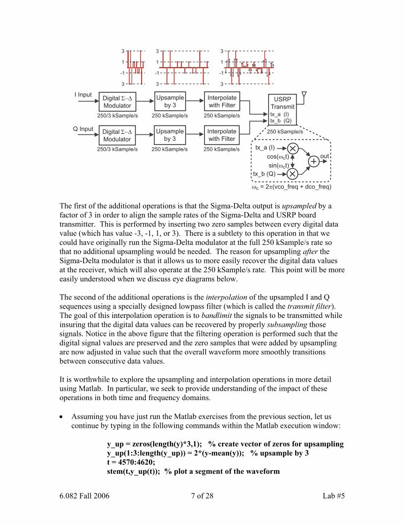
B. Upsampling and Interpolation for Data Transmission The figure below shows a more detailed view of how the digital transmitter will be implemented in code for this lab. The I and Q inputs will correspond to two different songs. The Sigma-Delta modulators are used to create 2-bit/symbol digital signals that represent the two input songs. The ouputs of the Sigma-Delta modulators are then sent through two additional operations before being sent to the USRP board for transmission, as now discussed.

6.082 Fall 2006 7 of 28 Lab #5

USRP

Transmittx_a (I)

tx_b (Q)

250 kSample/s

3

1

-1

3

3

1

-1

3

3

1

-1

3

Digital Σ−∆Modulator

250/3 kSample/s

Upsample

by 3

Interpolate

with Filter

250 kSample/s 250 kSample/s

I Input

Digital Σ−∆Modulator

250/3 kSample/s

Upsample

by 3

Interpolate

with Filter

250 kSample/s 250 kSample/s

Q Input

cos(ωct)

sin(ωct)

tx_a (I)

tx_b (Q)

out

ωc = 2π(vco_freq + dco_freq)

The first of the additional operations is that the Sigma-Delta output is upsampled by a factor of 3 in order to align the sample rates of the Sigma-Delta and USRP board transmitter. This is performed by inserting two zero samples between every digital data value (which has value -3, -1, 1, or 3). There is a subtlety to this operation in that we could have originally run the Sigma-Delta modulator at the full 250 kSample/s rate so that no additional upsampling would be needed. The reason for upsampling after the Sigma-Delta modulator is that it allows us to more easily recover the digital data values at the receiver, which will also operate at the 250 kSample/s rate. This point will be more easily understood when we discuss eye diagrams below. The second of the additional operations is the interpolation of the upsampled I and Q sequences using a specially designed lowpass filter (which is called the transmit filter). The goal of this interpolation operation is to bandlimit the signals to be transmitted while insuring that the digital data values can be recovered by properly subsampling those signals. Notice in the above figure that the filtering operation is performed such that the digital signal values are preserved and the zero samples that were added by upsampling are now adjusted in value such that the overall waveform more smoothly transitions between consecutive data values. It is worthwhile to explore the upsampling and interpolation operations in more detail using Matlab. In particular, we seek to provide understanding of the impact of these operations in both time and frequency domains. • Assuming you have just run the Matlab exercises from the previous section, let us

continue by typing in the following commands within the Matlab execution window: y_up = zeros(length(y)*3,1); % create vector of zeros for upsampling y_up(1:3:length(y_up)) = 2*(y-mean(y)); % upsample by 3 t = 4570:4620; stem(t,y_up(t)); % plot a segment of the waveform

6.082 Fall 2006 8 of 28 Lab #5

You should see a plot as shown below. Note that the Sigma-Delta output has now been modified to include two zero samples between every digital value.

• Let us now examine the fft of the upsampled signal by typing: f = (0:length(y_up)-1)*250e3/length(y_up) - 250e3/2; plot(f,abs(fftshift(fft(y_up)))) The resulting plot should appear as shown below:

6.082 Fall 2006 9 of 28 Lab #5

o A very important characteristic of upsampling is seen in the above fft plot, namely that the expansion of the samples in time leads to a compression of the frequency content of the resulting upsampled signal. In particular, notice that the above fft waveform corresponds to 3 shifted replicas of the fft of the original (i.e., non-upsampled) signal. Intuitively, we do not need to retain the newly added frequency content in order to keep all of the relevant information about the signal. In fact, since we do not want to use more spectrum than needed when transmitting the signal, it makes sense to consider filtering out the added frequency content. This provides motivation for doing interpolation, as now discussed.

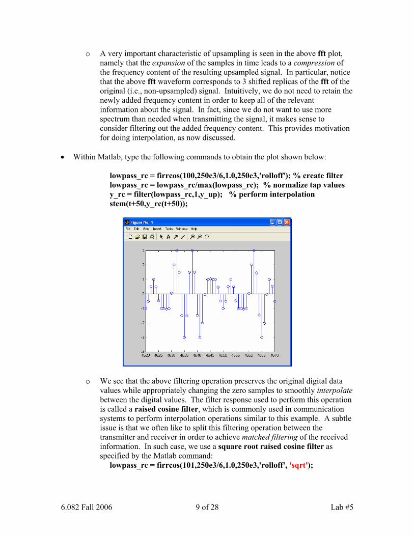
• Within Matlab, type the following commands to obtain the plot shown below: lowpass_rc = firrcos(100,250e3/6,1.0,250e3,'rolloff'); % create filter lowpass_rc = lowpass_rc/max(lowpass_rc); % normalize tap values y_rc = filter(lowpass_rc,1,y_up); % perform interpolation stem(t+50,y_rc(t+50));

o We see that the above filtering operation preserves the original digital data values while appropriately changing the zero samples to smoothly interpolate between the digital values. The filter response used to perform this operation is called a raised cosine filter, which is commonly used in communication systems to perform interpolation operations similar to this example. A subtle issue is that we often like to split this filtering operation between the transmitter and receiver in order to achieve matched filtering of the received information. In such case, we use a square root raised cosine filter as specified by the Matlab command:

lowpass_rc = firrcos(101,250e3/6,1.0,250e3,'rolloff', 'sqrt');

6.082 Fall 2006 10 of 28 Lab #5

instead of the raised cosine filter used above. In fact, we will actually make use of the square root raised cosine filter for both the transmitter and receiver in lab. These issues are discussed in more detail in advanced classes such as 6.011.

• Let us now examine the impact of the above operation in the frequency domain by

typing the Matlab command: plot(f,abs(fftshift(fft(y_rc)))) You should see a plot as shown below:

o We see that the interpolation operation filtered out much of the high frequency content, therefore achieving a more compact spectrum for the transmitted signal. We could have, in fact, filtered the signal even more while still preserving its key information. In the case of commercial applications, we would certainly do so since available spectrum is scarce. However, more aggressive filtering leads to more difficult recovery of the digital values at the receiver (due to higher sensitivity when trying to appropriately subsample the received waveform), and so we shall stick with less aggressive filtering in this lab in order to simplify implementation of the receiver. We will explore this issue further as we discuss eye diagrams below.

C. Eye Diagrams and Constellation Diagrams In order to efficiently examine waveforms associated with digital communication systems, it is desirable to add two useful tools to our arsenal. Eye diagrams are applied to the upsampled/interpolated signals discussed in the previous section and are used to

6.082 Fall 2006 11 of 28 Lab #5

provide an intuitive picture of how accurately we can recover the digital data values from subsampling such signals. Constellation diagrams are applied to the resulting subsamples, and provide us with a complementary view of the accuracy of the digital data recovery process.

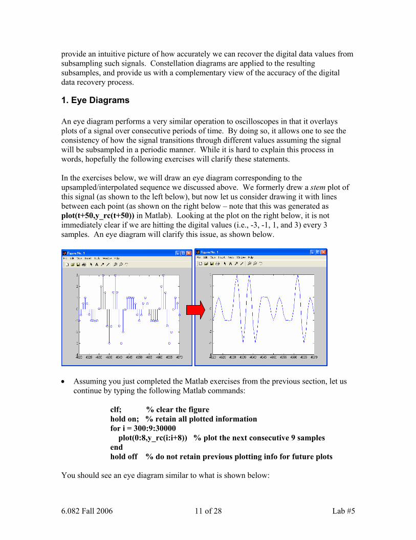
1. Eye Diagrams An eye diagram performs a very similar operation to oscilloscopes in that it overlays plots of a signal over consecutive periods of time. By doing so, it allows one to see the consistency of how the signal transitions through different values assuming the signal will be subsampled in a periodic manner. While it is hard to explain this process in words, hopefully the following exercises will clarify these statements. In the exercises below, we will draw an eye diagram corresponding to the upsampled/interpolated sequence we discussed above. We formerly drew a stem plot of this signal (as shown to the left below), but now let us consider drawing it with lines between each point (as shown on the right below – note that this was generated as plot(t+50,y_rc(t+50)) in Matlab). Looking at the plot on the right below, it is not immediately clear if we are hitting the digital values (i.e., -3, -1, 1, and 3) every 3 samples. An eye diagram will clarify this issue, as shown below.

• Assuming you just completed the Matlab exercises from the previous section, let us continue by typing the following Matlab commands:

clf; % clear the figure hold on; % retain all plotted information for i = 300:9:30000 plot(0:8,y_rc(i:i+8)) % plot the next consecutive 9 samples end hold off % do not retain previous plotting info for future plots You should see an eye diagram similar to what is shown below:

6.082 Fall 2006 12 of 28 Lab #5

o To understand the above diagram, first notice that the code consecutively plots every nine samples while preserving all previous plots. We know that the upsampled/interpolated waveform y_rc should have a digital value (i.e., either -3, -1, 1, or 3) every 3 samples. Looking at the above diagram, notice that at sample offsets of 0, 3, and 6, we do indeed see values that are restricted to these four possibilities. The sample points between these sample offsets correspond to the interpolated values that provide smooth progression between the digital values.

o Examination of the above eye diagram allows us to intuitively see the accuracy of recovering the digital data values by subsampling and slicing the y_rc waveform. We know that we want to subsample by a factor of 3, and we also want to slice in amplitude to decide which digital value occurred. The eye diagram indicates what sampling offset and slicing levels are appropriate. As an example, consider the sample offset and slicing levels shown below:

6.082 Fall 2006 13 of 28 Lab #5

0 1 2 3 4 5 6 7 8-4

-3

-2

-1

0

1

2

3

sample offset

am

plit

ud

e

Sample offset = 3

Slicing level = 2

Slicing level = 0

Slicing level = -2

o The above diagram reveals that we can very accurately determine whether the

digital value was -3, -1, 1, or 3 by using a sample offset of 3 and slice levels of -2, 0, and 2. As an example if the given sample value is below -2, we can be confident that the value is actually -3. If the given sample is between 0 and 2, we can be confident the value is actually 1. Note that we have equivalent results if we use a sample offset of 0 or 6, as well.

o Consider the alternative sample offset and slicing levels show below:

0 1 2 3 4 5 6 7 8-4

-3

-2

-1

0

1

2

3

sample offset

am

plit

ude

Sample offset = 4

Slicing level = 1.5

Slicing level = 0

Slicing level = -1.5

o As seen above, choosing a sample offset of 4 makes prevents accurate estimation of digital values since some of their corresponding trajectories fail to stay on their given side of the slicing level. As an example, we see that a slicing level of 1.5 is the best we can do to choose between a 1 or 3 value, but some trajectories from each of these values meet at the slicing level. As a result, one would expect that the wrong value would often be chosen in such cases, which would, in turn, lead to significant bit errors.

o In practice, a receiver would be able to choose sample offsets across a range of values that are not restricted to be integer in value. The above eye diagram

6.082 Fall 2006 14 of 28 Lab #5

reveals that the digital values can be retrieved for sample offsets that nearly span the range from 2 to 4. Therefore, in this case, the receiver is allowed a reasonable range of margin in choosing its sample offset, which thereby simplifies its design.

• The eye diagram is a useful tool to allow us to evaluate the impact of using a different

interpolation filter with respect to the ease of retrieving the digital values from the upsampled/interpolated signal. Let us continue with our Matlab exercises by performing filtering of our previously generated upsampled signal, y_up, with a raised cosine filter of lower bandwidth:

lowpass_rc = firrcos(100,250e3/6,0.3,250e3,'rolloff'); % new filter lowpass_rc = lowpass_rc/max(lowpass_rc); % normalize tap values y_rc = filter(lowpass_rc,1,y_up); % perform interpolation plot(f,abs(fftshift(fft(y_rc))))

o You should see an fft plot similar to what is shown below. Note that we have significantly reduced the spectral bandwidth of the upsampled/interpolated signal compared to the example in the previous section, which would be very advantageous for making the best use of available spectrum when transmitting. However, there is a cost to the reduced bandwidth with respect to retrieving the digital information from the signal, which is best explained by looking at the associated eye diagram of this new upsampled/interpolated signal.

o Now plot the eye diagram using the same set of Matlab commands used previously to achieve a similar plot to what is shown below:

% plot eye diagram as before clf; hold on;

6.082 Fall 2006 15 of 28 Lab #5

for i = 300:9:30000 plot(0:8,y_rc(i:i+8)) end hold off;

o Examination of the above plot reveals that the eye diagram is now much more closed than before. In particular, we notice that the range of possible sample offsets for accurate recovery of the digital values is much more restricted than in our previous example. When non-ideal effects of the communication channel and receiver are included (such as noise and additional filtering), the eye will further close and make recovery of the digital values even more challenging. Therefore, the receiver will need to be much more complex to properly retrieve the desired digital information from a more bandlimited signal.

o Thus far we have considered only one channel, but typical wireless communication systems have two channels (i.e., I and Q). In such case, analysis using eye diagrams requires one eye diagram per channel.

2. Constellation Diagrams Constellation diagrams allow an intuitive assessment of the ability to recover the digital data values from a received waveform after it has been sampled. In truth, eye diagrams provide all of the information conveyed by constellation diagrams and more since they also show the impact of different sample offsets. However, the value of constellation diagrams is in their simplicity, especially in viewing the effectiveness of a receiver in recovering the digital data values from both I and Q channels. We will explain this tool further through the use of Matlab exercises to follow. • Continuing with the Matlab exercises from above, let us first sample the previously

generated y_rc signal and then plot the resulting values to form the constellation

6.082 Fall 2006 16 of 28 Lab #5

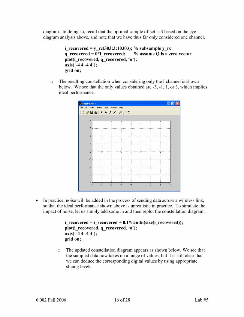
diagram. In doing so, recall that the optimal sample offset is 3 based on the eye diagram analysis above, and note that we have thus far only considered one channel.

i_recovered = y_rc(303:3:10303); % subsample y_rc q_recovered = 0*i_recovered; % assume Q is a zero vector plot(i_recovered, q_recovered, ‘o’); axis([-4 4 -4 4]); grid on;

o The resulting constellation when considering only the I channel is shown below. We see that the only values obtained are -3, -1, 1, or 3, which implies ideal performance.

• In practice, noise will be added in the process of sending data across a wireless link, so that the ideal performance shown above is unrealistic in practice. To simulate the impact of noise, let us simply add some in and then replot the constellation diagram:

i_recovered = i_recovered + 0.1*randn(size(i_recovered)); plot(i_recovered, q_recovered, ‘o’); axis([-4 4 -4 4]); grid on;

o The updated constellation diagram appears as shown below. We see that the sampled data now takes on a range of values, but it is still clear that we can deduce the corresponding digital values by using appropriate slicing levels.

6.082 Fall 2006 17 of 28 Lab #5

o To get a better understanding of the meaning of the above constellation diagram, plot the sampled i_recovered signal in time to obtain the plot shown below. Comparing this waveform to the above constellation diagram highlights the fact that the constellation diagram simply corresponds to a record of all possible values obtained for the sampled data stream over the entire time considered.

plot(i_recovered, ‘o’);

• It is much more common to consider both I and Q channels when forming the

constellation diagram. In order to do this exercise efficiently, we will create a fake Q

6.082 Fall 2006 18 of 28 Lab #5

signal by simply sampling the y_rc signal at a later sample offset than used to create the above I signal.

q_recovered = y_rc(603:3:10603) + 0.1*randn(size(i_recovered)); plot(i_recovered, q_recovered, 'o');

o The resulting I/Q constellation diagram should appear similar to what is shown below. We see from the diagram that we can faithfully determine the actual digital values for both I and Q channels through appropriate setting of slicing levels. In addition, it should be intuitive that higher noise levels will cause the deviations from the ideal values to increase. At a high enough noise level, it will no longer be possible to recover the actual digital value with certainty, and bit errors will result.

6.082 Fall 2006 19 of 28 Lab #5

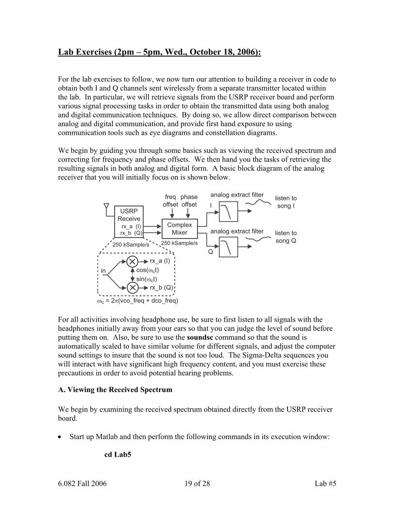
Lab Exercises (2pm – 5pm, Wed., October 18, 2006): For the lab exercises to follow, we now turn our attention to building a receiver in code to obtain both I and Q channels sent wirelessly from a separate transmitter located within the lab. In particular, we will retrieve signals from the USRP receiver board and perform various signal processing tasks in order to obtain the transmitted data using both analog and digital communication techniques. By doing so, we allow direct comparison between analog and digital communication, and provide first hand exposure to using communication tools such as eye diagrams and constellation diagrams. We begin by guiding you through some basics such as viewing the received spectrum and correcting for frequency and phase offsets. We then hand you the tasks of retrieving the resulting signals in both analog and digital form. A basic block diagram of the analog receiver that you will initially focus on is shown below.

USRP

Receiverx_a (I)

rx_b (Q)

250 kSample/s

Complex

Mixer

250 kSample/s

cos(ωct)

sin(ωct)

rx_a (I)

rx_b (Q)

in

ωc = 2π(vco_freq + dco_freq)

freq

offset

phase

offset I

Q

listen to

song I

listen to

song Q

analog extract filter

analog extract filter

For all activities involving headphone use, be sure to first listen to all signals with the headphones initially away from your ears so that you can judge the level of sound before putting them on. Also, be sure to use the soundsc command so that the sound is automatically scaled to have similar volume for different signals, and adjust the computer sound settings to insure that the sound is not too loud. The Sigma-Delta sequences you will interact with have significant high frequency content, and you must exercise these precautions in order to avoid potential hearing problems.

A. Viewing the Received Spectrum We begin by examining the received spectrum obtained directly from the USRP receiver board. • Start up Matlab and then perform the following commands in its execution window: cd Lab5

6.082 Fall 2006 20 of 28 Lab #5

system(‘initialize_usrp.exe’); %% initializes USRP board edit monitor_receive.m

o You should see a Matlab script as shown below. In essence, this script simply performs a loop operation in which data is obtained from the USRP receiver board and its fft computed and plotted. The USRP is set to downconvert signals that are centered at 457 MHz (i.e., vco_freq + dco_freq). The signal rx_a corresponds to the received I channel, and the signal rx_b corresponds to the received Q channel. We combine these signals into a complex signal, rx_a + j*rx_b, before plotting the corresponding fft. The use of a complex signal allows a more accurate picture of the signal spectrum (since it allows its fft to be non-symmetric about positive and negative frequencies, as we will see below). Also, complex notation will simplify the frequency and phase offset correction to be done in the next section.

vco_freq = 452e6; dco_freq = 5e6; adc_gain = 0; %% range is 0 to 20 dB mixer_gain = -30; %% range is -30 to 40 dB record_length = 50e3; f = (0:(record_length-1))*250e3/record_length – 250e3/2; for i = 1:1000 [rx_a,rx_b] = rf_receive(vco_freq, dco_freq, adc_gain, mixer_gain, record_length); plot(f,db(abs(fftshift(fft(rx_a+j*rx_b))))); axis([-125e3 125e3 -80 40]); drawnow end

• Execute the monitor_receive script in Matlab. You should see an fft plot similar to what is shown below. Note that the fft plot is not symmetric about positive and negative frequencies, and you can see that there is an offset in frequency if you look closely.

6.082 Fall 2006 21 of 28 Lab #5

o Note that the above spectrum consists of the desired analog signal, quantization noise, and two pilot tones which will be used to estimate the frequency and phase offset.

• Consider disconnecting and then re-connecting the antenna on the USRP receive

board while examining the received spectrum. This simple exercise should help convince you that you are indeed receiving the shown signal in a wireless manner.

B. “Building” the Analog Receiver Let us now “build” the analog receiver shown previously and repeated below, which essentially consists of a complex mixer and lowpass filters. The goal is to listen to the two songs which are embedded within the I and Q channels of the received signal. We will provide a template for this receiver within which you will need to fill in some missing pieces.

USRP

Receiverx_a (I)

rx_b (Q)

250 kSample/s

Complex

Mixer

250 kSample/s

cos(ωct)

sin(ωct)

rx_a (I)

rx_b (Q)

in

ωc = 2π(vco_freq + dco_freq)

freq

offset

phase

offset I

Q

listen to

song I

listen to

song Q

analog extract filter

analog extract filter

6.082 Fall 2006 22 of 28 Lab #5

• Within Matlab, examine the starting template of the analog receiver by typing: edit analog_receiver.m

o You should see the file shown below: vco_freq = 452e6; dco_freq = 5e6; adc_gain = 0; %% range is 0 to 20 dB mixer_gain = -30; %% range is -30 to 40 dB num_records = 20; record_length = 50e3; rx_a = zeros(1,num_records*record_length); rx_b = zeros(1,num_records*record_length); %%% receive data from USRP receiver board for i = 1:num_records [rx_a_s,rx_b_s] = rf_receive(vco_freq, dco_freq, adc_gain, mixer_gain, record_length); rx_a((1+(i-1)*record_length):(i*record_length)) = rx_a_s; rx_b((1+(i-1)*record_length):(i*record_length)) = rx_b_s; end %%% create time vector for use below t = (1:length(rx_a))/250e3; %%% calculate static frequency offset and time-varying phase offset [freq_offset,phase_offset] = calc_freq_and_phase_offset(rx_a,rx_b); %%% shift input in frequency and phase rx_demod = (rx_a + j*rx_b).*exp(j*(2*pi*(???)*t - ???)); %%% filter out quantization noise analog_extract_filt = fir1(100,???); i_analog_data = filter(analog_extract_filt,1,???); q_analog_data = filter(analog_extract_filt,1,???); %%% listen to a given channel soundsc(i_analog_data,250e3); • Fill in the missing items and execute the script in Matlab. Repeat until you

successfully hear the songs on both I and Q channels. At that point, call over a TA or instructor so that they can check you off on completing the analog receiver.

6.082 Fall 2006 23 of 28 Lab #5

C. “Building” the Digital Receiver Although the analog receiver is certainly functional, we can improve the performance of the receiver by making use of the fact that we can remove noise by retrieving the original digital values through appropriate subsampling and slicing. In this section you will build a digital version of the receiver, look at its corresponding eye diagrams and constellation diagrams, and then listen to the corresponding songs on the I and Q channels. We will simplify your task in doing so by providing some key Matlab functions and a starting Matlab script. However, you will need to figure out how to use and place those functions appropriately within the script. A basic view of the digital receiver is shown below. The initial portion is the same as the analog receiver, which is followed by matched filters on the I and Q channels which consist of square root raised cosine filters. The output of the matched filters, i_raw and q_raw, are sent into digital processing blocks which appropriately subsample and slice the data in order to produce signals i_sliced_data and q_sliced_data (which ideally match the original digital data sequences created by the Sigma-Delta modulator on the transmitter). The analog information is then extracted by the sliced data sequences by filtering out the quantization noise. Since the slicing operation in the digital processing section removes noise added by the wireless channel and receiver, the resulting audio quality should be improved compared to the analog version of the receiver.

USRP

Receiverx_a (I)

rx_b (Q)

250 kSample/s

Complex

Mixer

250 kSample/s

cos(ωct)

sin(ωct)

rx_a (I)

rx_b (Q)

in

ωc = 2π(vco_freq + dco_freq)

freq

offset

phase

offset I

Q

listen to

song I

listen to

song Q

analog extract filter

analog extract filter

matchedfilter

matchedfilter

Digital

receiver

operations

i_sliced_data

q_sliced_data

i_raw

q_raw

In order to assist you in performing the required digital receiver operations, several useful Matlab functions have been included in the Lab5 folder that you have been working in:

• [out] = sample_and_normalize_data(in) • [out] = slice_sampled_data(in) • plot_eye_diagram(in_i, in_q, start_symbol, num_symbols);

o For this exercise, start_symbol=10000 and num_symbols=10000 To examine the Matlab code corresponding to each of the above functions, simply edit their corresponding file (i.e., edit sample_and_normalize_data.m) within Matlab. Note

6.082 Fall 2006 24 of 28 Lab #5

that you will not need to change the code for any of the functions – examination of their content will simply help you to understand the operations they perform. • Within Matlab, edit digital_receiver.m to see the file shown below: vco_freq = 452e6; dco_freq = 5e6; adc_gain = 0; %% range is 0 to 20 dB mixer_gain = -30; %% range is -30 to 40 dB num_records = 20; record_length = 50e3; rx_a = zeros(1,num_records*record_length); rx_b = zeros(1,num_records*record_length); %%% receive data from USRP receiver board for i = 1:num_records [rx_a_s,rx_b_s] = rf_receive(vco_freq, dco_freq, adc_gain, mixer_gain, record_length); rx_a((1+(i-1)*record_length):(i*record_length)) = rx_a_s; rx_b((1+(i-1)*record_length):(i*record_length)) = rx_b_s; end %%% create time vector for use below t = (1:length(rx_a))/250e3; %%% calculate static frequency offset and time-varying phase offset [freq_offset,phase_offset] = calc_freq_and_phase_offset(rx_a,rx_b); %%% shift input in frequency and phase rx_demod = (rx_a + j*rx_b).*exp(j*(2*pi*(???)*t - ???)); %% this matched filter does not precisely match transmit filter, but %% is instead chosen for easy subsampling implementation below matched_filt = firrcos(100,250e3/4,0.7,250e3,'rolloff','sqrt'); %%% filter by matched filter i_raw = filter(matched_filt,1,???); q_raw = filter(matched_filt,1,???); %%%%%%% digital receiver operations %%%%%%% %%%%%%%%%%%%%%%%%%%%%%%%%%

6.082 Fall 2006 25 of 28 Lab #5

%%% filter out quantization noise analog_extract_filt = fir1(100,???); i_analog_data = filter(analog_extract_filt,1,i_sliced_data); q_analog_data = filter(analog_extract_filt,1,q_sliced_data); %%% listen to a given channel soundsc(i_analog_data,250e3); • Your first task is to fill in the missing parameters to allow you to compute i_raw and

q_raw. Once you have produced these signals, display their eye diagram to see the quality of your received signal. You should see eye diagrams similar to the ones shown below. If you do not, you may want to re-run the receive code several times. If that fails, you have likely messed something up in your script. Once you have a reasonable looking eye diagrams for the I and Q channels, call over a TA or instructor so that they can check you off on this portion of the lab.

• Now perform the digital processing steps needed to obtain a constellation diagram.

You should see something similar to what is shown below. Once you have the constellation diagram, call over a TA or instructor so that they can check you off on this portion of the lab.

6.082 Fall 2006 26 of 28 Lab #5

• Finally, fill in the digital processing code to produce signals i_sliced_data and

q_sliced_data. Plot the constellation diagrams of these signals and also listen to them in the headphone after you have filtered out the quantization noise. Call over a TA or instructor to check off this portion of the lab once you are done.

6.082 Fall 2006 27 of 28 Lab #5

Check-off for Lab 5

___________________________________ __________________________________ Student Name Partner Name Analog receiver:

Successfully extracted I/Q songs: ___________________________

Digital receiver:

Successfully obtained I/Q eye diagrams: ___________________________

Successfully obtained constellation diagram: ___________________________ Successfully extracted I/Q songs: ___________________________

6.082 Fall 2006 28 of 28 Lab #5

Postlab Answer the following questions individually and turn into class on Friday, Oct 20.

1. Given that a Sigma-Delta sequence has been used to encode a song: a. What operation needs to be done to extract the song content so that you

can listen to it? b. What sort of tradeoffs are involved in that operation?

2. In the Prelab, we stated that you needed to upsample and interpolate the Sigma-Delta sequence before sending it to the USRP transmit board.

a. Why was upsamping required? b. Why was interpolation required? c. Would you need to do either of these operations if you only wanted to do

analog modulation? Why? 3. When choosing a transmit filter:

a. Is it better to choose a low bandwidth or high bandwidth if the receiver complexity can be high? Why?

b. Is it better to choose a low bandwidth or high bandwidth if the receiver complexity must be low? Why?

4. What advantages does digital modulation have over analog modulation? 5. Why is it necessary to subsample and slice the received signal when doing digital

demodulation? 6. What desirable characteristics do you look for in an eye diagram when trying to

recover the original digital data stream at the receiver? 7. What desirable characteristics do you look for in a constellation diagram when

trying to recover the original data stream at the receiver? 8. Did you see evidence of bit errors when doing the digital demodulation? What

particular tool or test made this issue clear? 9. In the lab, what practical issues on the USRP board caused the frequency and

phase offset which needed to be removed?