massively parallel domain decomposition...

Massively Parallel Domain DecompositionPreconditioner for the High-Order Galerkin Least

Squares Finite Element Method

Masayuki Yano

Massachusetts Institute of TechnologyDepartment of Aeronautics and Astronautics

January 26, 2009

M. Yano (MIT) Qualifier Examination January 26, 2009 1 / 67

Outline

1 Introduction

2 High-Order Galerkin Least Squares

3 Balancing Domain Decomposition by Constraint

4 Results

5 Conclusion and Future Work


Outline

1 Introduction



4 Results



Motivation

Discretization RequirementsDiscretization should support

High-Order: Simulation of unsteady flows with multiple scalesbenefits from higher-order methods

Turbulence (DNS/LES)Acoustics / wave propagationEven in steady aerodynamics, high-order methods are moreefficient in terms of error/DOF [Barth, 1997][Venkatakrishnan, 2003]

Unstructured Mesh: Handling complex geometries

Selected Previous Work on High-Order MethodsHigh-order schemes have been designed for various frameworks

Finite difference [Lele, 1992]Finite volume [Barth, 1993][Wang, 2004]Finite element [Babuska, 1981][Patera, 1984]


Motivation

Example: High-Order Discretization

Drag convergence for NACA0012 [Fidkowski, 2005]

Decay of turbulent kinetic energyin LES modeling [Kosovic, 2000]

High-order schemes can significantly improve time to achieveengineering required accuracy.


Motivation

Massively Parallel AlgorithmsModern supercomputers are massively parallel (1000+ procs).Parallelization is essential for problems of practical interests.

Flow over large, complex geometriesUnsteady simulations (e.g. DNS/LES)

Trend of High Performance Computing in Past 15 Years

1994 1996 1998 2000 2002 2004 2006 200810

8

1010

1012

1014

1016

FLO

PS

Statistics from Top500.org

Cart3D

FUN3DJNWT

#1#500Average

1994 1996 1998 2000 2002 2004 2006 200810

0

102

104

106

Pro

cess

ors

Statistics from Top500.org

Cart3DFUN3D

JNWT

LargestSmallestAverage


Motivation

High-Performance Computing in Aeronautics

Typical large jobs remain in O(100) procs.

Range of scales present in viscous flows requires implicit solvers

“The scalability of most of [CFD] codes tops out around 512 cpus...” [Mavriplis, 2007]Exceptions:

FUN3D inviscid matrix-free Newton-Krylov-Schwarz solver using2048 procs [1999]Cart3D inviscid multigrid-accelerated Runge-Kutta solver using2048 procs [2005]NSU3D RANS multigrid solver with line implicit solver in boundarylayers using 2048 procs [2005]

Need highly scalable implicit solver to take advantage of the futurecomputers with 10,000+ procs.


Objectives and Approaches

Objectives1 High-order discretization on unstructured mesh2 Highly scalable solution algorithm for massively parallel systems

Approaches1 Galerkin Least Squares (GLS)

Study behavior of high-order GLS discretization.Use h/p scaling artificial viscosity for subcell shock capturing.

2 Domain Decomposition (DD) PreconditionerSolve Schur complement system using preconditioned GMRESbased on DD.Test the preconditioner for high-order discretization ofadvection-dominated flows.


Outline

1 Introduction



4 Results



Galerkin Least Squares Discretization

BackgroundStabilized FEM for advection-dominated flows

SUPG developed by Hughes [1982]; analyzed by Johnson [1984]

SUPG extended to GLS by Hughes [1989]

GLS Discretization for Advection-DiffusionDifferential operator and bilinear form

Lu ≡ β · ∇u −∇ · (ν∇u) = f

a(u, φ) = (β · ∇u, φ)Ω + (ν∇u,∇φ)Ω, ∀u, φ ∈ V ⊂ H1(Ω)

Find u ∈ V s.t.

a(u, φ) + (Lu, τLφ)Ω,Th= (f , φ)Ω + (f , τLφ)Ω,Th

, ∀φ ∈ V

where (·, ·)Ω,Th =∑

K

∫

K · · dK and τ ∼(

h, Pe ≫ 1

h2, Pe ≪ 1.


Stabilization Matrix

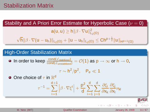
Stability and A Priori Error Estimate for Hyperbolic Case (ν = 0)

a(u,u) ≥ h‖β · ∇u‖2L2(Ω)

√h‖β · ∇(u − uh)‖L2(Ω) + ‖u − uh‖L2(Ω) ≤ Chp+ 1

2‖u‖Hp+1(Ω)

High-Order Stabilization Matrix

In order to keep cond(Lstabilized)cond(Lunstabilized)

= O(1) as p → ∞ or h → 0,

τ ∼ h2/p2, Pe ≪ 1

One choice of τ in Rd

τ−1 =

d+1∑

i=1

∣

∣

∣β · ∇ξi

∣

∣

∣+

p2

d

d∑

i=1

d∑

j=1

∂ξi

∂xk

∂ξj

∂xlνkl


Outline

1 Introduction



4 Results



Domain Decomposition Preconditioners

MotivationPerformance of ILU degrades with number of processors evenwith line partitioning [Diosady, 2007].

Data parallelism alone is not sufficient to obtain good performancein massively parallel environment (1000+ procs.)

Selected Previous Work (Elliptic)Bourgat proposesNeumann-Neumann method forSchur complement system [1988].

Mandel improves scalability withBalancing DD [1993].

Dorhmann extends BDD to BDDC[2003].


Schur Complement System

Discrete Harmonic Extension (Elliptic Equation)Decompose Ω into non-overlapping domains Ωi and defineΓi = ∂Ωi \ ∂Ω and Γ = ∪N

i=1Γi . Decompose Vh ⊂ H1(Ω) into

Vh(Ω \ Γ) = v ∈ Vh : v |Γ = 0Vh(Γ) = v ∈ Vh : a(v , φ) = 0,∀φ ∈ Vh(Ω \ Γ)

Vh(Γ) is called the space of discrete harmonic extensions.

Variational ProblemFind u = u + u ∈ Vh(Ω \ Γ) ⊕ Vh(Γ) s.t.

a(u, ψ) = (f , ψ)Ω, ∀ψ ∈ Vh(Ω \ Γ)

a(u, φ) = (f , φ)Ω, ∀φ ∈ Vh(Γ)

u requires local Dirichlet solves

u requires global interface solve

Ωi

Ωk

Ωj

Γ


Schur Complement System

Schur Complement Operator

Schur complement operator S : Vh(Γ) → Vh(Γ)′ defined by

〈Sv , φ〉 = a(v , φ), ∀v , φ ∈ Vh(Γ)

where, 〈·, ·〉 : W ′ × W → R s.t. 〈F , v〉 ≡ F (v), ∀F ∈ W ′,∀v ∈ W .

Schur Complement Problem

Find u ∈ Vh(Γ) s.t.

〈Su, φ〉 = (f , φ)Ω , ∀φ ∈ Vh(Γ)

Forming S is expensive; action of S on v ∈ Vh(Γ) is computed vialocal Dirichlet solves and minimal communication.

Problem solved using a Krylov space method (e.g. GMRES)

Scalable preconditioner needed to accelerate convergence


BDDC Spaces

Features of BDDCEquipped with a coarse space that

makes subdomain problems wellposedprovides global communication

Example of primal constrainsValues at corners of Ωi

Averages on the edges of Ωi

SpacesVh(Γ) = global discrete harmonic extension

⊕Ni=1Vh(Γi) = collection of local discrete

harmonic extensions

(i.e. discontinuous across Γ)

Vh(Γ) = v ∈ ⊕Ni=1Vh(Γi) :

v continuous on primal constraints

Vh(Γ)

⊕Ni=1Vh(Γi)

Vh(Γ)M. Yano (MIT) Qualifier Examination January 26, 2009 16 / 67

BDDC Spaces

Vh(Γ)

Dual and Primal Spaces

Decompose Vh(Γ) into ⊕iVh,∆(Γi) andVh,Π(Γ).

Dual problems are decoupled

Primal problem has DOF of O(N)

Dual Space (∆):Vh,∆(Γi) = v ∈ Vh(Γi) :

v = 0 on primal constraint

Primal Space (Π):Vh,Π(Γ) = v ∈ Vh(Γ) :

X

Ni=1ai(v |Ωi , φ∆|Ωi ) = 0,

∀φ∆ ∈ ⊕Ni=1Vh,∆(Γi)


BDDC Preconditioner

Primal and Dual Schur Complement

Primal Schur complement: SΠ : Vh,Π(Γ) → V ′h,Π(Γ)

〈SΠvΠ, φΠ〉 =∑

Ni=1ai(v |Ωi , φ|Ωi ), ∀vΠ, φΠ ∈ Vh,Π(Γ)

Local dual Schur complement: S∆,i : Vh,∆(Γi) → V ′h,∆(Γi )

〈S∆,iv∆,i , φ∆,i〉 = ai(v∆,i , φ∆,i) ∀v∆,i , φ∆,i ∈ Vh,∆(Γi)

BDDC Preconditioner

M−1BDDC =

∑

Ni=1RT

D,i(Tsub,i + Tcoarse)RD,i

where Tsub,i = RTΓ∆,iS

−1∆,iRΓ∆,i and Tcoarse = RT

ΓΠS−1Π RΓΠ

Condition Number Estimate for Coercive, Symmetric a(·, ·)κ(M−1

BDDCS) ≤ C(1 + log2 (H/h))


Robin-Robin Interface Condition (IC)

BackgroundAdaptation of N-N condition to nonsymmetric bilinear form

Proposed by Achdou for BDD [1997]

Applied to FETI [Toselli, 2001] and BDDC [Tu, 2008]

Robin-Robin IC

Subtract∫

Γi

12β · niuφ from interfaces.

Modified local bilinear form is

ai(u, φ) = (ν∇u,∇φ)Ωi+ 1

2 (β · ∇u, φ)Ωi− 1

2 (β · ∇φ,u)Ωi

+ 12 (u, vβ · n)∂Ωi∩∂ΩN

ai(·, ·) is positive in local space Vh(Ωi): ai(u,u) ≥ ν|u|H1(Ωi ).

Resulting IC on Γi is Robin type(

ν∇u − 12β)

· n = 0 on Γi


Outline

1 Introduction



4 Results



Poisson Equation

Poisson Equation ObjectivesTest scaling with :

Number of subdomains

Size of subdomain

p for different primal constraints

Solution Partitioning Examples

0 0.2 0.4 0.6 0.8 10

0.1

0.2

0.3

0.4

0.5

0.6

0.7

0.8

0.9

1

0 0.2 0.4 0.6 0.8 10

0.1

0.2

0.3

0.4

0.5

0.6

0.7

0.8

0.9

1


Poisson Equation

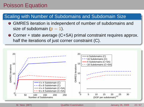
Scaling with Number of Subdomains and Subdomain SizeGMRES iteration is independent of number of subdomains andsize of subdomain (p = 1).

Corner + state average (C+SA) primal constraint requires approx.half the iterations of just corner constraint (C).

0 50 100 150 200 2500

5

10

15

20

Number of Subdomains

GM

RE

S it

erat

ions

4 x 4 Subdomain (C)8 x 8 Subdomain (C)4 x 4 Subdomain (C+SA)8 x 8 Subdomain (C+SA)

0 5 10 15 20 25 300

5

10

15

20

(DOF per subdomain)1/2

GM

RE

S it

erat

ions

4 Subdomains (C)16 Subdomains (C)4 Subdomains (C+SA)16 Subdomains (C+SA)


Poisson Equation

Scaling with pPoisson equation solved on unstructured mesh ∼ 8000 elem.

Number of iterations nearly independent of p when C+SA primalconstraints are used.

Size of Primal ProblemCorners only: ≈ Nsubdomain

Corners + Edge StateAverage: ≈ 3 × Nsubdomain

0 20 40 60 80 100 1200

5

10

15

20

25

30

35

40


GM

RE

S it

erat

ions

p = 1 (C)p = 4 (C)p = 1 (C+SA)p = 4 (C+SA)


Advection Diffusion: Boundary Layer

Boundary Layer Equation ObjectivesStudy effect of:

interface conditions (Neumann-Neumann vs. Robin-Robin)

τ scaling (h2 vs. h2/p2)

Solution (ν = 10−3) Anisotropic Mesh and Partitioning

0 0.2 0.4 0.6 0.8 10

0.1

0.2

0.3

0.4

0.5

0.6

0.7

0.8

0.9

1

0 0.2 0.4 0.6 0.8 10

0.1

0.2

0.3

0.4

0.5

0.6

0.7

0.8

0.9

1



Interface Conditions (IC)Robin-Robin IC performs significantly better thanNeumann-Neumann IC in advection dominated cases.

Interface conditions are identical as ν → ∞.

10−6

10−4

10−2

100

0

20

40

60

80

100

ν

GM

RE

S it

erat

ions

diffusionadvection

N−N (p=1)R−R (p=1)

10−6

10−4

10−2

100

20

40

60

80

100

120

140

ν

GM

RE

S it

erat

ions

diffusionadvection

N−N (p=1)R−R (p=1)

Nsubdomain = 16 Nsubdomain = 64



τ Matrix Scaling

Performance of preconditioner degrades for p > 1 if τ ∼ h2 indiffusion dominated cases.

With τ ∼ h2/p2, the preconditioner performs similar to p = 1 case.

10−6

10−4

10−2

100

0

5

10

15

20

25

30

35

ν

GM

RE

S it

erat

ions

diffusionadvection

p=1p=3, τ

v~h2

p=3, τv~h2/p2

Nsubdomain = 64


Outline

1 Introduction



4 Results



Conclusion and Future Work

ConclusionBDDC preconditioner shows good scalability for:

Both diffusion-dominated and advection-dominated flows withRobin-Robin interface conditionAll ranges of interpolation order p with proper choices of τ andprimal constraints

Future WorkExtension to 3D

Inexact solvers for subdomain problems

Complex geometries and highly anisotropic mesh


Questions

Supplemental Slides

Instability of the Standard Galerkin Method

DiscretizationAdvection-diffusion equation

Lu ≡ β · ∇u −∇ · (ν∇u) = f

Galerkin: Find u ∈ V ⊂ H1(Ω) s.t.

a(u, φ) = (f , φ)Ω, ∀φ ∈ V

where a(u, φ) =∫

Ω φβ · ∇u + ν∇φ · ∇u.

Stability and A Priori Error Estimate

a(u,u) ≥ ν‖∇u‖2L2(Ω) = ν|u|2H1(Ω)

ν|u − uh|H1(Ω) ≤ Chp‖u‖Hp+1(Ω)

Not coercive in H1(Ω) as ν → 0.

1D Boundary Layer

0 0.2 0.4 0.6 0.8 10

0.1

0.2

0.3

0.4

0.5

0.6

0.7

0.8

0.9

1

Pe = βh2ν = 1/4

0 0.2 0.4 0.6 0.8 10

0.2

0.4

0.6

0.8

1

1.2

1.4

1.6

1.8

Pe = 5


Stabilized Finite Element Methods

Stabilized Methods for Advection-Dominated FlowsStreamline-Upwind Petrov-Galerkin (SUPG) [Hughes 1982]

Galerkin Least-Squares (GLS) [Hughes 1989]

Residual Free Bubbles (RFB) [Brezzi 1994]

Variational Multiscale based on local Green’s function [Hughes1995]


Finite Element vs. Finite Volume

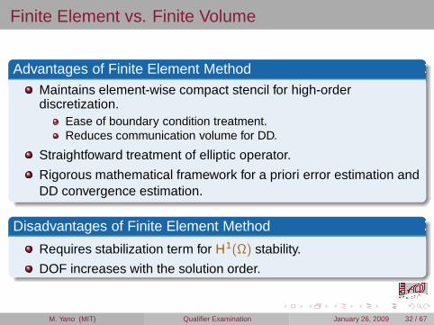
Advantages of Finite Element MethodMaintains element-wise compact stencil for high-orderdiscretization.

Ease of boundary condition treatment.Reduces communication volume for DD.

Straightfoward treatment of elliptic operator.

Rigorous mathematical framework for a priori error estimation andDD convergence estimation.

Disadvantages of Finite Element Method

Requires stabilization term for H1(Ω) stability.

DOF increases with the solution order.


High-Order Galerkin Basis

Basis Function TypesThree types of basis functions (in 2D): Node, Edge, Element.

Basis type defined by its support.

The continuity constraint must be enforced on nodal and edgebasis during assembly.

Node Edge Element


High-Order Galerkin: Matrix Storage

Object-based Block StorageJacobian stored blockwise, with the varying size of blocks

Matrix converted to CRS format before solved with UMFPACK

Jacobian of 3 × 3 Mesh (18 elem, p = 5, arbitrary basis)

0 50 100 150 200 250

0

50

100

150

200

250

nz = 7186

0 50 100 150 200 250 300 350

0

50

100

150

200

250

300

350

nz = 26460

Galerkin DG (with compact lifting)


Comparison with Discontinuous Galerkin

Features (common to DG)High-order discretization on unstructured mesh

H1(Ω) stability for advection-dominated flows

Advantages (compared to DG)Straightforward treatment of elliptic operators (no lifting required)

Fewer DOF required to represent a solution in H1(Ω)

DisadvantagesPotentially expensive calculation of stabilization terms

Absence of block-wise compact stencil (more complexpreconditioning strategy required)


High-Order SUPG vs. GLS

p-Refinement with Traditional τ

If h ≫ ν/‖β‖, SUPG p-refinement fails to converge.

Asymptotic convergence rates as h → 0 are identical(‖e‖H1(Ω) ∼ hp)

0.7 0.75 0.8 0.85 0.9 0.95 10

0.2

0.4

0.6

0.8

1

1.2

p=1p=3p=5p=7exact

0.7 0.75 0.8 0.85 0.9 0.95 10

0.2

0.4

0.6

0.8

1

1.2

p=1p=3p=5p=7exact

SUPG GLSSolution to advection-diffusion equation (h = 0.1, ν/‖β‖ = 0.01)


High-Order SUPG vs. GLS

p-Refinement with High-Order Modified τ

With the high-order modified τ , both SUPG and GLS p-refinementconverge to the exact solution.

GLS converges much rapidly than SUPG with p.

0.7 0.75 0.8 0.85 0.9 0.95 10

0.2

0.4

0.6

0.8

1

1.2

p=1p=3p=5p=7exact

0.7 0.75 0.8 0.85 0.9 0.95 10

0.2

0.4

0.6

0.8

1

1.2

p=1p=3p=5p=7exact

SUPG GLSSolution to advection-diffusion equation (h = 0.1, ν/‖β‖ = 0.01)


Shock Capturing

BackgroundArtificial viscosity can regularize underresolved features.

Method applied to DG by Persson [2006] and Barter [2007] toachieve subcell shock capturing.

Resolution Indicator and h/p-Scaling Artificial Viscosityhigh-order resolution indicator based on orthogonal polynomialexpansion [Persson, 2006]

Se =(u − Πp−1u,u − Πp−1u)K

(u,u)K, u ∈ Pp(K )

where Πp−1 is the L2(K ) projection onto Pp−1(K ).

If log10(Se) ≥ s0, add piecewise constant viscosity ν ∼ h/p to theelement.


Shock Capturing: Result

Burger’s EquationBurger’s equation solved on ≈ 450 element mesh.

∂

∂x

(

12

u2)

+∂u∂y

+ ∇ · (νartificial(u)∇u) = 0

0 0.5 1 1.50

0.5

1

1.5

Solution (p = 5) Resolution Indicator


Euler Equation: Gaussian Bump

FormulationSymmetric form using Hughes’ entropy variables [1986]

V =

(−s + γ + 1γ − 1

− ρEp,

ρui

p, − ρ

p

)

The governing equation becomesA0V,t + AiV,xi = 0

where A0 is SPD and Ai is symmetric (Kij is SPSD for N-S).

Gaussian Bump: Pressure and Partitioning


Euler Equation: Gaussian Bump

Euler EquationBDDC with R-R IC performs well for Euler equation.

With N-N IC, 400+ GMRES iteration required for 32 subdomains.

0 20 40 60 80 100 1200

10

20

30

40

50

60


GM

RE

S it

erat

ions

20 elem/subdom (p=1)20 elem/subdom (p=3)80 elem/subdom (p=1)

Average of GMRES iterations required for last three Newton steps


Parallel Scalability of ILU

Scalability of ILU for DG Discretization [Diosady 2007]Navier-Stokes equation

Partitioning based on line connectivity

Line-ordered ILU with p-Multigrid within each subdomain

0 2 4 6 8 10 12 14 160

100

200

300

400

500

600Linear Iterations vs. Number of Processors

Number of Processors

Line

arIte

ratio

ns

NoneLines

0 2 4 6 8 10 12 14 160

2

4

6

8

10

12

14

16Speed Up vs Number of Processors

Number of Processors

Spe

edup

NoneLines

Iterations vs. Processors Parallel Speed-Up


Schur Complement for Non-Self-Adjoint Operator

Discrete Harmonic Extension (Non-Self-Adjoint)

Decompose Vh ⊂ H1(Ω) into

Vh(Ω \ Γ) = v ∈ Vh : v |Γ = 0Vh(Γ) = v ∈ Vh : a(v , φ) = 0,∀φ ∈ Vh(Ω \ Γ)V ∗

h (Γ) = ψ ∈ Vh : a(w , ψ) = 0,∀w ∈ Vh(Ω \ Γ)

Find u = u + u ∈ Vh(Ω \ Γ) ⊕ Vh(Γ) s.t.

a(u, φ) = (f , φ)Ω, ∀φ ∈ Vh(Ω \ Γ)

a(u, ψ) = (f , ψ)Ω, ∀ψ ∈ V ∗h (Γ)

Schur Complement Operator

Schur complement S : Vh(Γ) → V ∗h (Γ)′ s.t.

〈Sv , ψ〉 = a(v , ψ), ∀v ∈ Vh(Γ), ∀ψ ∈ V ∗h (Γ)


Neumann-Neumann Preconditioner

Local Spaces and Local Schur Complement

Decompose Vh(Ωi) ⊂ H1(Ωi) of Ωi intoVh(Ωi \ Γi) = vi ∈ Vh(Ωi ) : v |∂Ωi = 0Vh(Γi ) = vi ∈ Vh(Ωi) : ai(vi , φ) = 0, ∀φ ∈ Vh(Ωi \ Γi)Local Schur complement: Si : Vh(Γi ) → Vh(Γi)

′

〈Sivi , φi〉 = ai(vi , φi), ∀vi , φi ∈ Vh(Γi)

Interpolation and Weighting Function

Interpolation: RTi : Vh(Γi) → Vh(Γ) s.t.

⊕Ni=1RT

i Vh(Γi) = Vh(Γ)

Weighting Function: Di ∈ Vh(Γi) s.t.

Di = 1/(# of Ωi sharing DOF on Γ)

Note, v =∑

Ni=1RT

i Div |Ωi ,∀v ∈ Vh(Γ)

Vh(Γ)

⊕Ni=1Vh(Γi )


Neumann-Neumann Preconditioner

Neumann-Neumann (N-N) Preconditioner

Precondition S by applying S−1i : V ′(Γi) → V (Γi) on each Ωi and

interpolate the result back to V (Γ)

M−1NN =

∑

Ni=1RT

i DiS−1i DiRi

For ai(u, φ) = (∇u,∇φ)Ωi , application of S−1i corresponds to

solving a local problem with Neumann interface condition on Γi

(∇u) · n = 0 on Γi


NNS) ≤ CH2 (1 + log(H/h))2


Balancing Domain Decompositions

Problems of Neumann-Neumann PreconditionerLocal Schur complement Si may be singular

Limited scalability due to lack of coarse space

Coarse SpaceIntroduce coarse space Vh,0 that

makes subdomain problems well-posed

provides global communication

DOFcoarse = O(N)

Examples of DD with a Coarse SpaceBDD: Balancing Domain Decomposition [Mandel, 1993]

BDDC: BDD by Constraints [Dohrmann, 2003]


Balancing Domain Decomposition

Balancing Domain Decomposition

Define a coarse space: Vh,0(Ω) = span

RTi δ

†i

, Kernel(Si) ⊂ Vh,0

Define projection P0 : Vh(Ω) → Vh,0(Ω), P0 = RT0 S−1

0 R0S

Apply Neumann-Neumann preconditioner to balanced problem

M−1BDD = RT

0 S−10 R0 + (I − P0)

(

∑

Ni=1RT

i DiS−1i DiRiS

)

(I − P0)

Examples of DD with a Coarse SpaceBDD: Balancing Domain Decomposition [Mandel, 1993]

Vh,0 = ⊕Ni=1Kernel(Si).

Apply multiplicative coarse correction such that residual ofsubdomain problem is in range(Si ). (i.e. ’balanced’ problem)

BDDC: BDD by Constraints [Dohrmann 2003]Vh,0 = Ψi, harmonic extensions satisfying primal constraints.Solve additive coarse and constrained subdomain problems.


Comparison of Primal and Dual SubstructuringMethods

Primal TypePreconditions the Schur complement system by solving Neumannproblems using the flux jumps.

Neumann-Neumann method [Bourgat 1988]

Balancing Domain Decomposition (BDD) [Mandel, 1993]

BDD by Constraints (BDDC) [Dohrmann 2003]

Dual TypePreconditions the flux equations by solving Dirichlet problems usingfunction jumps.

Finite Element Tearing and Interconnecting (FETI) [Farhat 1991]Dual-Primal FETI (FETI-DP) [Farhat 2001]

Spectrum of BDDC and FETI-DP preconditioned operators areidentical [Mandel 2005][Li 2005]


BDDC Spaces

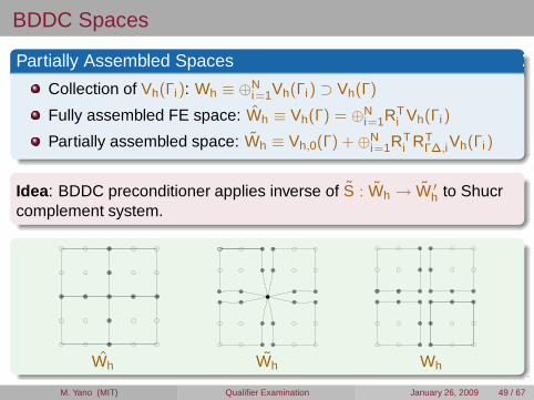
Partially Assembled Spaces

Collection of Vh(Γi): Wh ≡ ⊕Ni=1Vh(Γi) ⊃ Vh(Γ)

Fully assembled FE space: Wh ≡ Vh(Γ) = ⊕Ni=1RT

i Vh(Γi)

Partially assembled space: Wh ≡ Vh,0(Γ) + ⊕Ni=1RT

i RTΓ∆,iVh(Γi)

Idea: BDDC preconditioner applies inverse of S : Wh → W ′h to Shucr

complement system.

Wh Wh Wh


Schur Complement System: Matrix Form

Schur ComplementDecompose local stiffness matrix and load vector into

A(i) =

(

A(i)II A(i)

IΓ

A(i)ΓI A(i)

ΓΓ

)

and f (i) =

(

f (i)I

f (i)Γ

)

Schur complement system is given by

SuΓ = g

where

S =

N∑

j=1

R(j),T S(j)R(j), S(j) = A(j)ΓΓ − A(j)

ΓI

(

A(j)II

)−1A(j)

IΓ

g =

N∑

j=1

R(j),T g(j), g(j) = f (j)Γ − A(j)

ΓI

(

A(j)II

)−1f (j)I


Application of Schur Complement

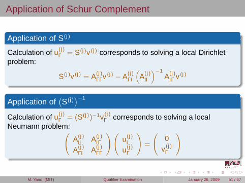
Application of S(j)

Calculation of u(j)Γ = S(j)v (j) corresponds to solving a local Dirichlet

problem:

S(j)v (j) = A(j)ΓΓv (j) − A(j)

ΓI

(

A(j)II

)−1A(j)

IΓ v (j)

Application of(

S(j))−1

Calculation of u(j)Γ = (S(j))−1v (j)

Γ corresponds to solving a localNeumann problem:

(

A(j)II A(j)

IΓ

A(j)ΓI A(j)

ΓΓ

)(

u(j)I

u(j)Γ

)

=

(

0v (j)Γ

)


BDDC: Coarse Correction

Coarse CorrectionCoarse-level correction operator is given by

Tcoarse = Ψ(ΨT SΨ)−1ΨT

whereΨ ≡

(

Ψ(1),T , · · · ,Ψ(N),T)T

∈ RDOF(⊕Vh(Γi ))×Nprimal

Coarse Basis

The local coarse basis, Ψ(i) is the harmonic extension to Ωi thatsatisfies the primal constraints, i.e.

(

S(i) C(i),T

C(i) 0

)(

Ψ(i)

Λ(i)

)

=

(

0

R(i)Π

)

where C(i) enforces primal constraints and Λ(i) is Lagrange multiplier.


BDDC: Subdomain Correction

Subdomain CorrectionSubdomain correction is given by

Tsub =N∑

i=1

(

R(i),TΓ 0

)

(

S(i) C(i),T

C(i) 0

)−1(

R(i)Γ0

)

Provides subdomain corrections for which all coarse level, primalvariables vanish.

Primal constraints ensure the local problem is invertible.


BDDC: Change of Basis

Idea [Klawonn, 2004]Change basis functions on interface to make primal constraintsexplicit.

Removes the need for the Lagrange multipliers as primalcontinuity constraints are satisfied by construction.

Example: State AverageChange of basis ψk → ψl such that

Dual Variables:∫

edge ψl(ξ)dξ = 0, l = 1, . . . ,n − 1Primal Variable: ψn(ξ) = 1, ∀ξ ∈ edge

Let TCOB be the weighting matrix that maps from ψ to φ, then newstiffness matrix is

Aψ,ij = a(ψi , ψj ) = (T TCOBAφTCOB)i ,j


Abstract Additive Schwarz Preconditioner

AssumptionConsider symmetric, coercive a(·, ·) : V → V and ai(·, ·) : Vi → Vi .Assume ∃C0, ω, E = (ǫij)

Ni ,j=1 such that

Stable Decomposition

∀v ∈ V ,∃vi ∈ Vi :∑

Ni=0ai(vi , vi) ≤ C0a(v , v)

Local Stability

∀i = 1, . . . ,N,∀vi ∈ Vi : a(vi , vi ) ≤ ωai(vi , vi)

Strengthened Cauchy-Shwarz Inequality

∀i , j = 1, . . . ,N,∀ui ∈ Vi ,∀vj ∈ Vj : |a(ui , vj)| ≤ ǫij

√

a(ui ,ui)a(vj , vj )

Conditioner Number Estimate [Dryja, 1995]

κ ≤ C0ω (1 + ρ(E))


BDDC Condition Number Estimate

Rayleigh Quotient

Applying Rayleigh quotient formula to the inner product 〈MBDDC·, ·〉,

λmin

(

M−1BDDCS

)

= minv 6=0

〈Sv , v〉minv=RT

D RTΓΠvΠ+

PNi=1 RT

D,iRTΓ∆,i v∆,i

vΠ∈Vh,Π(Γ),v∆,i∈Vh,∆(Γi )

(

〈SΠvΠ, vΠ〉 +∑N

i=1〈S∆,i v∆,i , v∆i 〉)

λmax

(

M−1BDDCS

)

= maxv 6=0

〈Sv , v〉minv=RT

D RTΓΠvΠ+

PNi=1 RT

D,iRTΓ∆,i v∆,i


(

〈SΠvΠ, vΠ〉 +∑N

i=1〈S∆,i v∆,i , v∆i 〉)


Eigenvalues: Lower Bound

Schur Complement on Vh(Γ)

〈Sv , φ〉 =∑

Ni=1ai (v |Ωi , φ|Ωi ) , ∀v , φ ∈ Vh(Ω)

Derivation

〈SΠvΠ, vΠ〉 +∑

Ni=1〈S∆,i v∆,i , v∆,i〉 = 〈SvΠ, vΠ〉 +

∑

Ni=1ai (v∆,i , v∆,i)

= 〈SvΠ, vΠ〉 + 〈Sv∆, v∆〉= 〈S(vΠ + v∆), (vΠ + v∆)〉 = 〈Sv , v〉

〈Sv , v〉 ≥ minv=RT

D RTΓΠvΠ+

PNi=1 RT

D,iRTΓ∆,i v∆,i


(

〈SΠvΠ, vΠ〉 +N∑

i=1

〈S∆,iv∆,i , v∆i 〉)

λmin

(

M−1BDDCS

)

≥ 1


Eigenvalues: Upper Bound

Derivation

〈Sv , v〉 ≤ 2[〈SRTD RT

ΓΠvΠ,RTD RT

ΓΠvΠ〉+ 〈S(

∑

Ni=1RT

D,iRTΓ∆,iv∆,i), (

∑

Ni=k RT

D,k RTΓ∆,k v∆,k )〉]

. 〈SRTD RT

ΓΠvΠ,RTDRT

ΓΠvΠ〉 +∑

Ni=1〈S(RT

D,i RTΓ∆,iv∆,i), (R

TD,i R

TΓ∆,iv∆,i)〉

For symmetric, coercive bilinear form with p = 1,

〈SRTD RT

ΓΠvΠ,RTD RT

ΓΠvΠ〉 . (1 + log2(H/h))〈SΠvΠ, vΠ〉〈S(RT

D,iRTΓ∆,iv∆,i), (RT

D,iRTΓ∆,iv∆,i)〉 . (1 + log2(H/h))〈S∆,i v∆,i , v∆,i〉

Thus,〈Sv , v〉 .

„

1 + log2„

Hh

««

minv=RT

D RTΓΠvΠ+

PNi=1 RT

D,i RTΓ∆,i v∆,i


〈SΠvΠ, vΠ〉 +NX

i=1

〈S∆,iv∆,i , v∆i 〉

!

λmax

(

M−1BDDCS

)

≤ C(

1 + log2(H/h))


BDDC: GMRES Convergence Estimate

GMRES Residual Bound [Eisenstat, 1983]

Let c anc C2 be such that

c0〈u,u〉 ≤ 〈u,Tu〉〈Tu,Tu〉 ≤ C2

0〈u,u〉

Then,‖rm‖‖ro‖

≤(

1 − c20

C20

)m/2

Advection-Diffusion Convergence Estimate [Tu, 2008]With state and flux average as primal constraints, BDDC (R-R)satisfies

c0 = 1 − CH(H/h)(1 + log(H/h))

C0 = C(1 + log(H/h))4


Nonlinear Equation Solution Scheme

Discrete form using Galerkin Method

MhdUh

dt+ Rh(Uh(t)) = 0

Time Stepping Scheme

Um+1h = Um

h −(

1∆t

Mh +∂Rh

∂Uh

)−1

Rh(Umh )

For steady problems ∆t → ∞.

Linear SystemAhxh = bh must be solved at each time step

A =1∆t

Mh +∂Rh

∂Uhx = ∆Um

h b = −Rh(Umh )


Parallel GLS Solver

GLS Solver FeaturesMany ideas borrowed from ProjectX (Discontinuous Galerkinsolver developed at ACDL since 2002)

High-order GLS discretization on unstructured mesh

h/p-scaling artificial viscosity for shock capturing.

Parallel communication via MPI

Local direct solve using UMFPACK

Equation set: Poisson, advection-diffusion, Burger, Euler

∼ 70,000 lines of C code


BDDC Spaces

Primal and Dual Spaces

Decompose Vh(Γ) = (Vh,Π(Γ)) ⊕ (⊕Ni=1Vh,∆(Γi))

Local Dual: Vh,∆(Γi ) = v ∈ Vh(Γi ) : v = 0 on primal constraintPrimal: Vh,Π(Γ) = v ∈ Vh(Γ) :

∑

Ni=1ai (v |Ωi , φ∆|Ωi ) = 0,

∀φ∆ ∈ ⊕Ni=1Vh,∆(Γi)

Dual space Vh,∆(Γ) = ⊕Ni=1Vh,∆(Γi ) is completely localized

Primal space has DOF of O(N)

Primal and Dual Schur Complement

Primal Schur complement: SΠ : Vh,Π(Γ) → V ′h,Π(Γ)

〈SΠvΠ, φΠ〉 =∑

Ni=1ai(v |Ωi , φ|Ωi ), ∀vΠ, φΠ ∈ Vh,Π(Γ)

Local dual Schur complement: S∆,i : Vh,∆(Γi) → V ′h,∆(Γi )

〈S∆,iv∆,i , φ∆,i〉 = ai(v∆,i , φ∆,i) ∀v∆,i , φ∆,i ∈ Vh,∆(Γi)


BDDC Preconditioner

Injections and Averaging Operator

RTΓΠ : Vh,Π(Γ) → Vh(Γ)

RTΓ∆ : Vh,∆(Γi) → Vh(Γ)

RTD,i : Vh(Γ) → Vh(Γ) s.t. v =

∑ Ni=1RT

D,iv |Ωi ,∀v ∈ Vh(Γ)

BDDC PreconditionerBDDC preconditioner is given by

M−1BDDC =

∑

Ni=1RT

D,i(Tsub,i + Tcoarse)DiRD,i

where Tsub,i = RTΓ∆,iS

−1∆,iRΓ∆,i and Tcoarse = RΓΠS−1

Π RTΓΠ


BDDCS) ≤ C(1 + log2 (H/h))


Galerkin Least Squares Discretization

BackgroundSUPG developed by Hughes [1982]; analyzed by Johnson [1984]

SUPG extended to GLS by Hughes [1989]

GLS Discretization

Find u ∈ V ⊂ H1(Ω) s.t.

a(u, φ) + (Lu, τLφ)Ω,Th= (f , φ)Ω + (f , τLφ)Ω,Th

, ∀φ ∈ V

where (·, ·)Ω,Th =∑

K

∫

K · · dK and τ ∼(

h, Pe ≫ 1

h2, Pe ≪ 1.

Stability and A Priori Error Estimate for Hyperbolic Case (ν = 0)

a(u,u) ≥ h‖β · ∇u‖2L2(Ω)

√h‖β · ∇(u − uh)‖L2(Ω) + ‖u − uh‖L2(Ω) ≤ Chp+ 1

2‖u‖Hp+1(Ω)


Stabilization Matrix

High-Order Stabilization Matrix

In order to keep cond(Lstabilized)cond(Lunstabilized)

= O(1) as p → ∞ and h → 0,

τ ∼ h2/p2, Pe ≪ 1

One choice of τ in Rd

τ−1 =d+1∑

i=1

∣

∣

∣β · ∇ξi

∣

∣

∣+

p2

d

d∑

i=1

d∑

j=1

∂ξi

∂xk

∂ξj

∂xlνkl

Topics Studied in High-Order GLSComparison of SUPG and GLS

Subcell-shock capturing using h/p scaling artificial viscosity andresolution based shock indicator

GLS for highly anisotropic mesh


BDDC Preconditioner

Features of BDDCEquipped with a coarse space (primal space) that provides globalcommunication and makes subdomain problems well-posed.

Operates on partially assembled space: Vh(Γ)

Vh(Γ) = v ∈ L2(Ω) : v ∈ ⊕Ni=1Vh(Γi)

and v is continuous on primal constraintsExamples of primal constraints

Values at the corners of Ωi

State averages on the edges of Ωi

Vh(Γ) Vh(Γ) ⊕Ni=1Vh(Γi)


BDDC Spaces

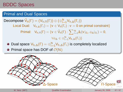
Primal and Dual Spaces

Decompose Vh(Γ) = (Vh,Π(Γ)) ⊕ (⊕Ni=1Vh,∆(Γi))

Local Dual: Vh,∆(Γi ) = v ∈ Vh(Γi ) : v = 0 on primal constraintPrimal: Vh,Π(Γ) = v ∈ Vh(Γ) :

∑

Ni=1ai (v |Ωi , φ∆|Ωi ) = 0,

∀φ∆ ∈ ⊕Ni=1Vh,∆(Γi)

Dual space Vh,∆(Γ) = ⊕Ni=1Vh,∆(Γi ) is completely localized

Primal space has DOF of O(N)

∆-Space Π-Space


massively parallel domain decomposition...

Documents