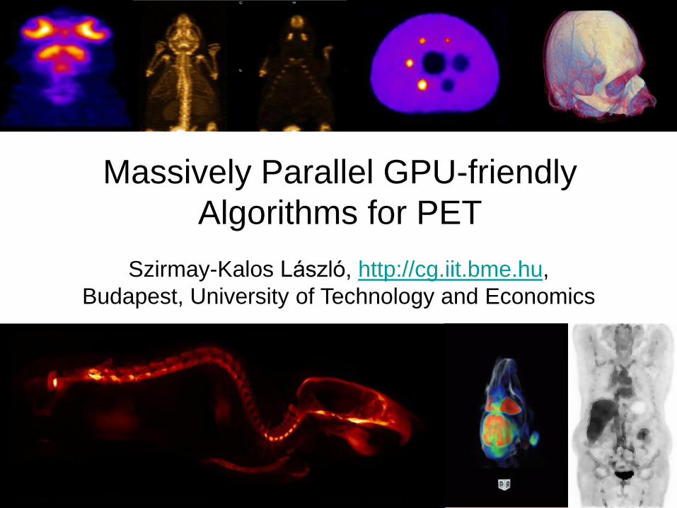
Massively Parallel GPU-friendly

Algorithms for PET

Szirmay-Kalos László, http://cg.iit.bme.hu,

Budapest, University of Technology and Economics

(GP)GPU: CUDA (OpenCL)

Multiprocessor N

Multiprocessor 2

Multiprocessor 1

Scalar

Processor

1

Shared memory

Scalar

Processor

M

Cache

Device memory

Instruction

Execution

Unit

• Massively parallel:

#threads > 104

• Independence:

synchronization and

write collisions should

be avoided

• SIMD: conditional

statements are not

welcome

• Coalesced memory

access

PET physics

Line Of Response

(LOR)

P

e-

e+PN

MedisonanoScan PET AnyScan PET

Maximum-likelihood reconstruction

x1 x2

x3 x4

Expected number of hits:

Maximize the probability of

the measurement data y:

A11

A13

A12

A14

xAy ~

414313

2121111~

xAxA

xAxAy

)}(~|Pr{maxarg xyyx

Iterative solution

Activity in voxels

Correction

Physics

Simulation

Measured

valuesExpected

values

Computational challenges

• Numbers of LORs and voxels: hundred millions!

• System matrix A: 1016 elements (PetaBytes)

– Probability that a positron of a voxel is detected by a LOR

– Patient dependent

– Not sparse if accurate simulation is needed

– Do not store, estimate on-the-fly

• Matrix elements are high dimensional integrals

– Monte Carlo quadrature

– Reuse of computation

– High performance (parallel) computational platform

• Minimize the effect of estimation error

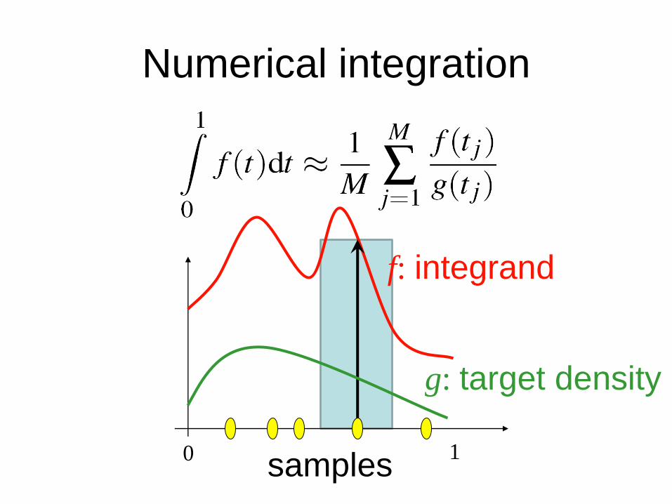
Numerical integration

0 1

f: integrand

g: target density

samples

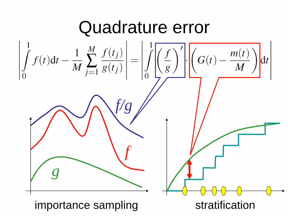
Quadrature error

f

g

f/g

importance sampling stratification

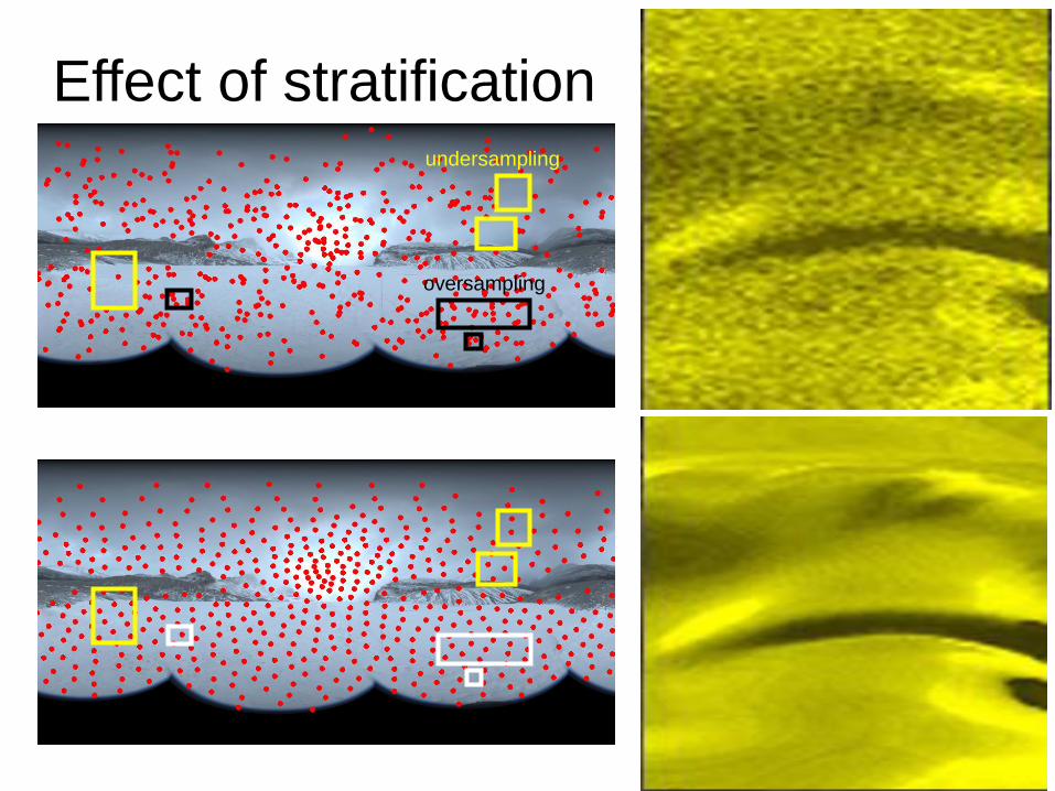
Effect of stratificationundersampling

oversampling

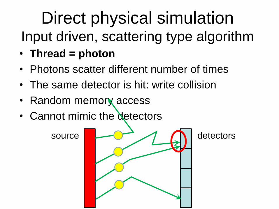
Direct physical simulationInput driven, scattering type algorithm• Thread = photon

• Photons scatter different number of times

• The same detector is hit: write collision

• Random memory access

• Cannot mimic the detectors

source detectors

GPU friendly approachOutput driven, gathering type

• Thread = importon

• SIMD: grouping importons

• No write collision: LOR-driven

• Cannot mimic the source

source detectors

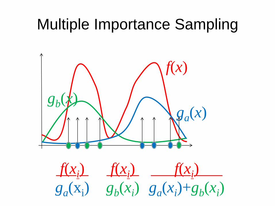
Multiple Importance Sampling

f(x)

ga(x)gb(x)

f(xi)

ga(xi)

f(xi)

gb(xi)

f(xi)

ga(xi)+gb(xi)

Direct gamma photon contribution

Detector

module 1

Detector

module 2

voxel

LOR

vvx dd )(

5D Integration

• Accuracy for given

sample number

• Cost of a sample

l

Output- or LOR-driven sampling

Detector

module 1

Detector

module 2

LOR

lwuGD

Nlg

),(),(

2

ray

1

Pros:

• Gathering

• Thread coherence

• Texture coherence

• Uniform on detectors

• Low-cost samples

due to reuse

Cons:

• Cannot mimick activityl

l

u

w

Input or voxel-driven sampling

Detector

module 1

Detector

module 2

LOR

Pros:

• Can mimick activity

Cons:

• Write collisions

• Less coherence

vxD

ullxNlg

d)cos(

)(),(

2

voxel

2

l

u

Multiple Importance Sampling

voxel voxel

+

lwuGD

Nlg

),(),(

2

ray

1

),(),(),( 21

lglglg

vxD

ullxNlg

d)cos(

)(),(

2

voxel

2

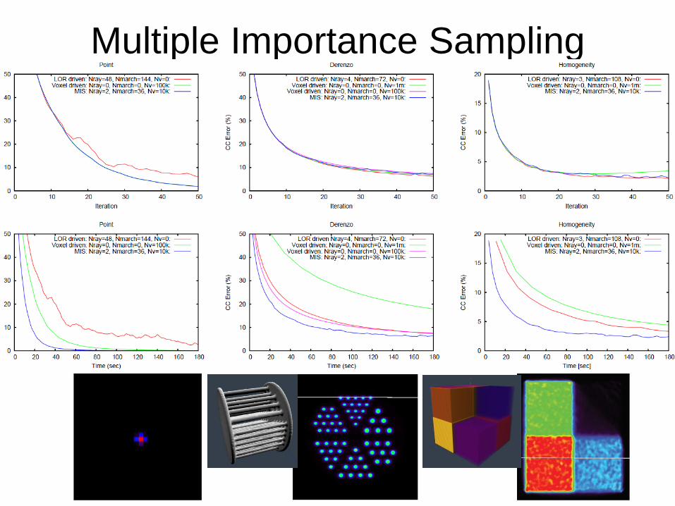
Multiple Importance Sampling

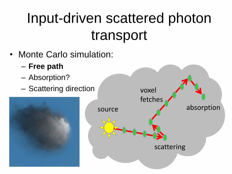
Input-driven scattered photon

transport

• Monte Carlo simulation:

– Free path

– Absorption?

– Scattering direction

source absorption

voxelfetches

scattering

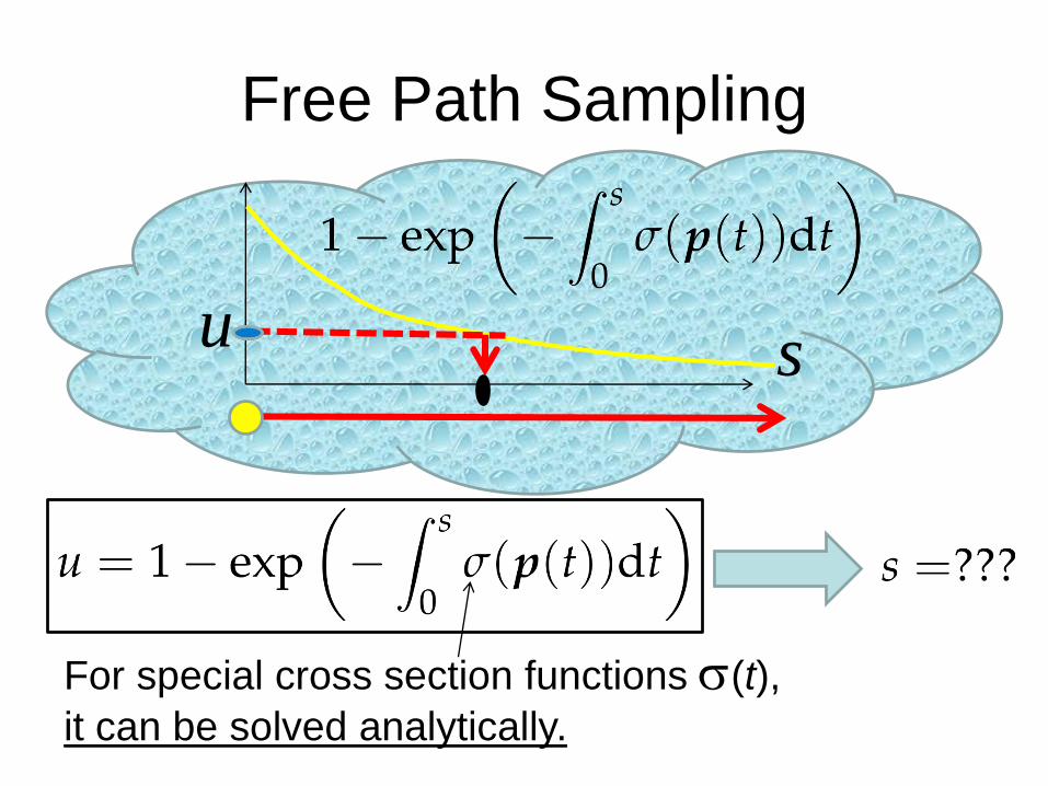
u s

Free Path Sampling

For special cross section functions (t),

it can be solved analytically.

Ray marching

• Complexity grows with the resolution

• Slow in high resolution low density media

)exp(1 si

i

u

Mix virtual particles to obtain a density

that can be solved analytically

photon

Virtual

collision

Real

collision

Virtual particleReal material

particle

40963 effective resolution

64 billion sample points

Output-driven single-scattered

photon transport with reuse

1z

1s

2s

1. Scattering points 2. Ray marching between

scattering points and detectors

1s

2s

1z

2z

3. Combination

1s

2s

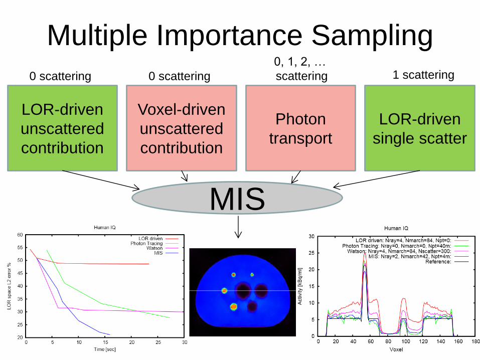
Multiple Importance Sampling

LOR-driven

unscattered

contribution

Voxel-driven

unscattered

contribution

Photon

transport

LOR-driven

single scatter

0 scattering 0 scattering

0, 1, 2, …

scattering 1 scattering

MIS

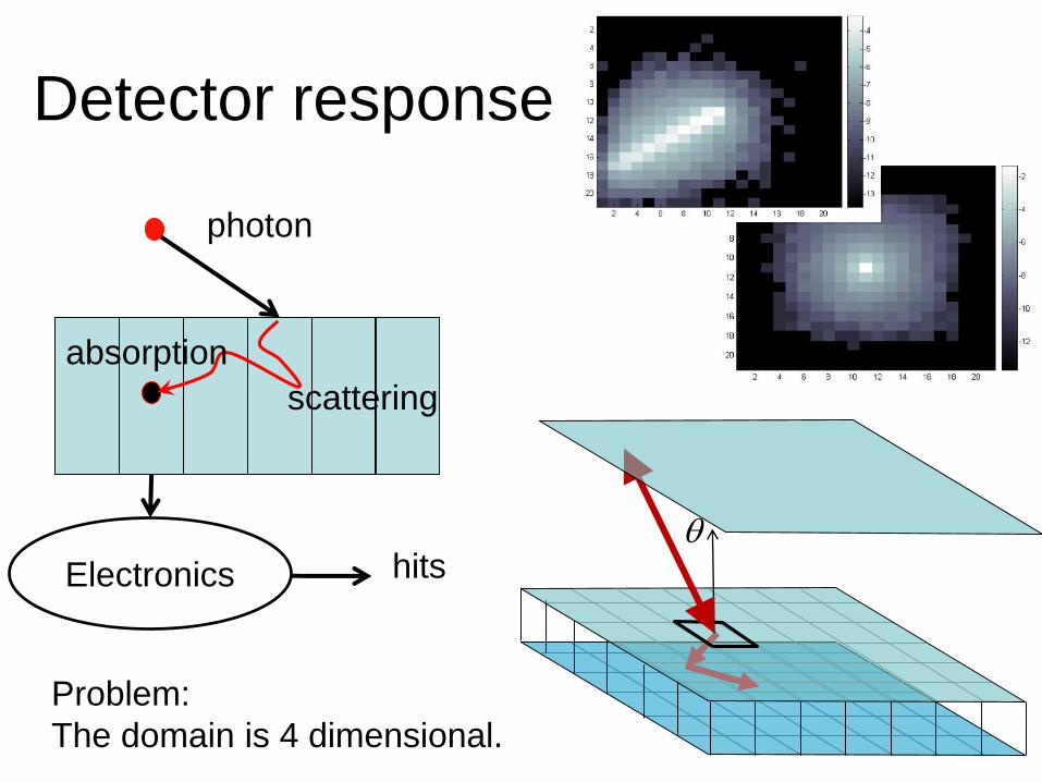
Detector response

photon

scattering

absorption

Electronics hits

Problem:

The domain is 4 dimensional.

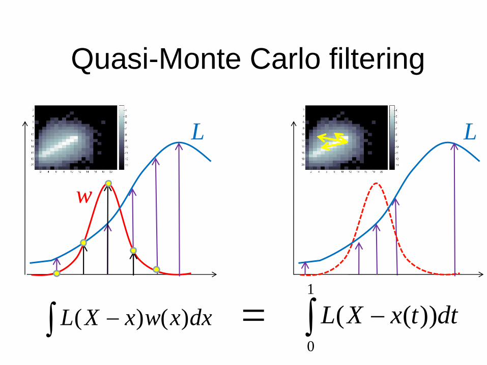
dxxwxXL )()(

1

0

))(( dttxXL

L

w

L

=

Quasi-Monte Carlo filtering

Detector Scattering Compensationw

ith

ou

t

with

Measured

values

voxels

Correction

Physics

Simulation

)()( xAy nn ~

Expected

values

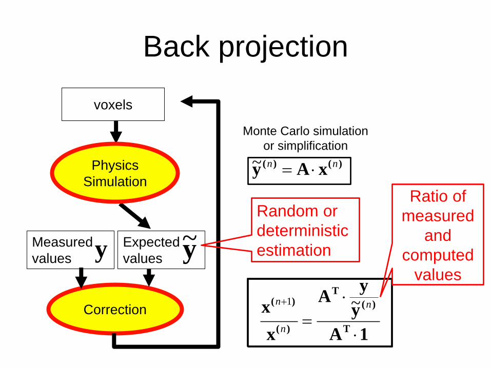
Back projection

Monte Carlo simulation

or simplification

Random or

deterministic

estimation

1A

y

yA

x

xT

)(

T

)(

)(

n

n

n ~1

y~y

Ratio of

measured

and

computed

values

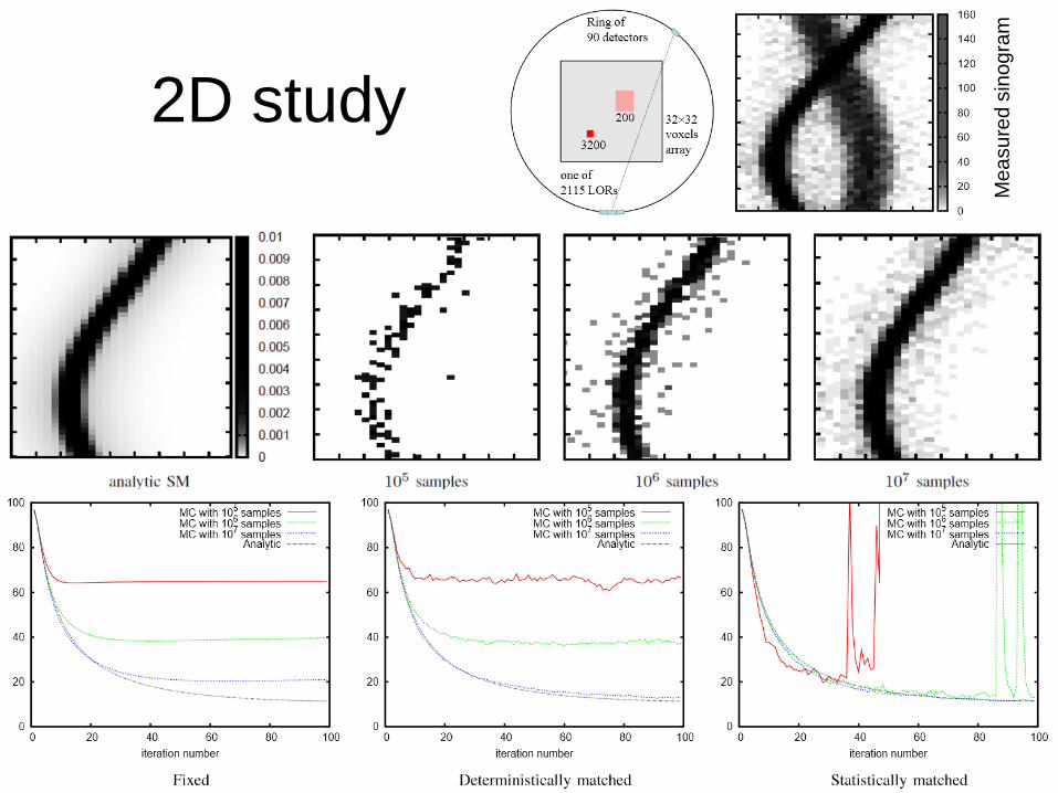
2D study

Me

asu

red

sin

og

ram

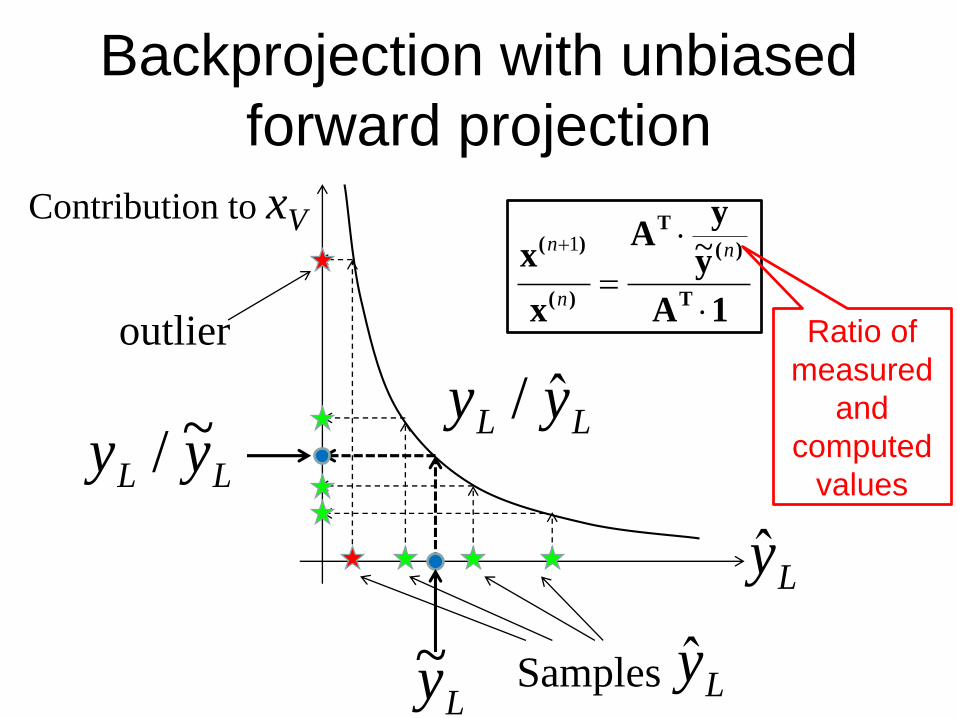
Backprojection with unbiased

forward projection

Contribution to xV

Samples

outlier1A

y

yA

x

xT

)(

T

)(

)(

n

n

n ~1

Ly~

Ly

Ly

LL yy ˆ/LL yy ~/

Ratio of

measured

and

computed

values

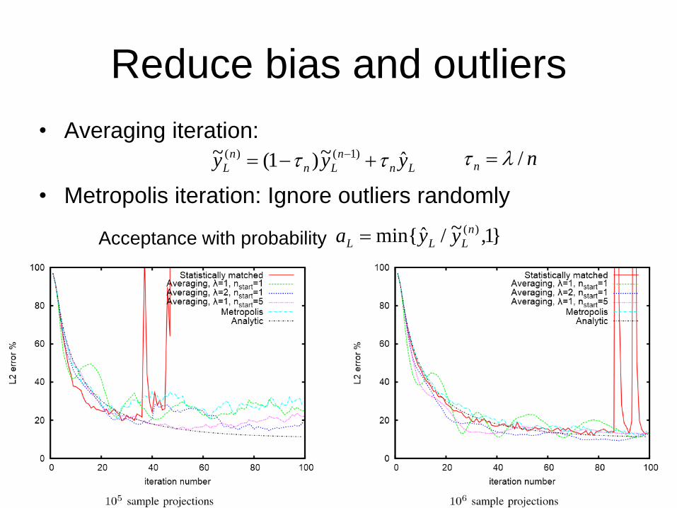
Reduce bias and outliers

• Averaging iteration:

• Metropolis iteration: Ignore outliers randomly

Acceptance with probability

nn / Ln

n

Ln

n

L yyy ˆ~)1(~ )1()(

}1,~/ˆmin{ )(n

LLL yya

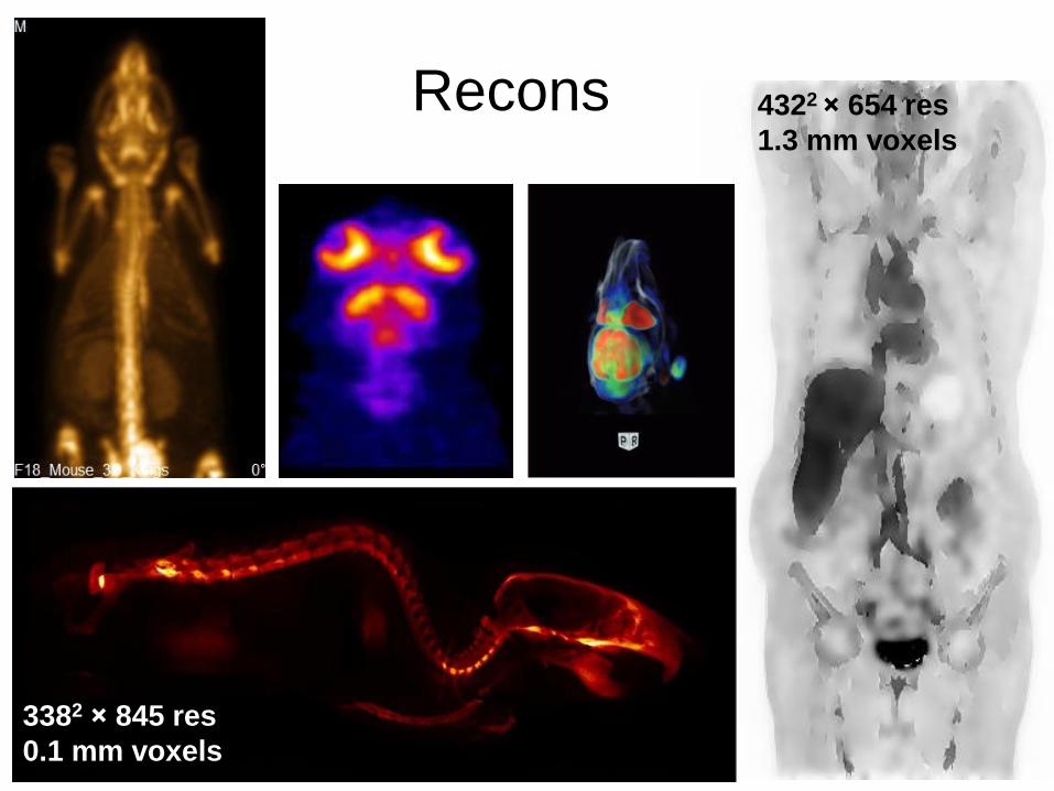
Recons

3382 × 845 res

0.1 mm voxels

4322 × 654 res

1.3 mm voxels

Conclusions

• GPU is an effective tool for computing tens

of thousands of parallel threads having no

conditionals and collisions.

• The problem must be interpreted and

solved to keep this requirement in mind.

• Randomization (Monte Carlo) can help

structure the problem in this way.