master of business administration bachelor of chemical ...683425/s42824822_phd... · a thesis...

1

Dynamic Analysis of Dense Medium Circuits

Nerrida Julienne Catherine Scott

Master of Business Administration

Bachelor of Chemical Engineering

Bachelor of Business Administration

A thesis submitted for the degree of Doctor of Philosophy at

The University of Queensland in 2017

Sustainable Minerals Institute

Julius Kruttschnitt Mineral Research Centre

2

Abstract

Dense Medium Cyclone (DMC) geometry and DMC performance have been widely

explored in the past. Some investigations have been made into the dynamic changes that

take place over a DMC circuit while the plant is running, however this has been limited by

the lack of on-line plant data. Understanding of the dynamics of the whole DMC circuit

requires further enquiry. This includes, following changes in medium density, medium to

coal ratio, %non-magnetics, velocities and pressures, classification and sizing of the

magnetite, the effects of bleeds and wing tank dynamics.

Plant operators typically run coal preparation plants to a set of conditions stipulated based

on mine yield/ash predictions, steady-state measurements and design parameters without

a full knowledge of how dynamic changes affect the DMC circuit. Essentially, they operate

the plant on a macro level, controlling tonnage, volume, and density cut point to align with

variations in plant feed. Furthermore, technology has limited operators’ ability to see the

subtle changes that occur in the dense medium, for example, when the circuit is unstable.

This project addresses those issues and should therefore be able to advance knowledge

in the area of dynamic analysis of dense medium cyclone circuits.

3

Declaration by author

This thesis is composed of my original work, and contains no material previously published

or written by another person except where due reference has been made in the text. I

have clearly stated the contribution by others to jointly-authored works that I have included

in my thesis.

I have clearly stated the contribution of others to my thesis as a whole, including statistical

assistance, survey design, data analysis, significant technical procedures, professional

editorial advice, and any other original research work used or reported in my thesis. The

content of my thesis is the result of work I have carried out since the commencement of

my research higher degree candidature and does not include a substantial part of work

that has been submitted to qualify for the award of any other degree or diploma in any

university or other tertiary institution. I have clearly stated which parts of my thesis, if any,

have been submitted to qualify for another award.

I acknowledge that an electronic copy of my thesis must be lodged with the University

Library and, subject to the policy and procedures of The University of Queensland, the

thesis be made available for research and study in accordance with the Copyright Act

1968 unless a period of embargo has been approved by the Dean of the Graduate School.

I acknowledge that copyright of all material contained in my thesis resides with the

copyright holder(s) of that material. Where appropriate I have obtained copyright

permission from the copyright holder to reproduce material in this thesis.

4

Publications during candidature

Scott,N., Holtham,P., Firth,B., O’Brien,M., (2013) On-line Simulation & Dynamic Analysis

of Dense Medium Cyclone Circuits., International Coal Preparation Congress, 2013,

Istanbul, Turkey.

Firth,B., O’Brien,M., Holtham,P., Scott,N., Hu,S., Dixon,R., Burger,A., (2014) Dynamic

Impacts of Plant Feed and Operating practices on a Dense Medium Cyclone (DMC)

Circuit, 15th Australian Coal Preparation Conference Proceedings 14-18th Sept 2014,

Gold Coast, Australia

Firth, B., Holtham,P., O’Brien, M., Hu,S., Dixon,R., Burger, A., Scott,N., Linkage of

Dynamic Changes in DMC Circuits to Plant Conditions, ACARP Report C50152, Australian

Coal Association Research Program, February 2013.

Scott,N., Wood,C., Holtham,P., O’Brien,M., Firth,B., (2015) Integration of Plant Residence

Time Measurement Into a Dynamic Model of a Coal Dense Medium Circuit, Coal Prep

2015, April 27-29th2015, Lexington, Kentucky, USA.

O’Brien,M., Firth,B., Holtham,P., Hu,S., Scott,N., Burger,A., Optimisation and Control of

Dense Medium Cyclone Circuits, International Coal Preparation Congress, July 2016, St

Petersburg, Russia

Publications included in this thesis

No publications included

5

Contributions by others to the thesis

A collaborative body of work has been ongoing between the University of Queensland and

CSIRO and a series of these ACARP sponsored projects preceded this project. The

technical and plant data collected was predominantly obtained by CSIRO/UQ coordinated

sampling campaigns in which I actively took part. Data was also collected from CSIRO

and UQ developed instruments and the New Acland plant instrumentation. Results of this

research have been shared amongst these organisations, however, some data remains

the property of CSIRO and New Acland mine and due to confidentiality cannot be

specifically detailed in this thesis.

I would like to acknowledge the assistance of CSIRO in providing laboratory resources,

training and technical support, and also the assistance of New Acland Coal Handling and

Preparation Plant for supporting access to their site for this research to take place. Their

assistance in finding and providing plant production information has been invaluable.

Collaborative efforts between CSIRO, UQ and New Acland are gratefully acknowledged,

particularly the assistance of Dr Peter Holtham, Dr Bruce Firth and Mr Michael O’Brien and

technical support from their team. Parallel research conducted by CSIRO in other ACARP

projects has been beneficial to this PhD.

I would also like to acknowledge the technical support of Partition Enterprises and

members of my fellow student cohort who assisted with RFID tracer testing and the

collection of standard tracers at the New Acland mine. Partition Enterprises also assisted

this PhD thesis by providing RFID tracer times collected from their instruments.

Statement of parts of the thesis submitted to qualify for the award of another degree

None

6

Acknowledgements

I would like to acknowledge the support of the following people and organisations:

My parents, Yvonne and Eric Scott – whom without their steadfast support through the ups

and downs, I could not have embarked nor continued on this journey. My brothers, Roger

and Stuart have also offered great moral support. Luke, my son, who was two years old

when I started this journey and who kindly offered to fix my simulation model at age 4 by

tickling my computer and purportedly doing magic has now reached the tender age of 7

years and has grown more than 30 centimetres in height since I started. His continual

streams of questions, amusing and insightful conversations have inspired me to keep on

learning and acquiring new knowledge, whatever my stage or circumstances in life.

Australian Coal Association Research Programme – Who generously funded the various

CSIRO / JKMRC research projects that contributed to this PhD and who also funded my

PhD Scholarship. ACARP continue to be wonderful supporters of coal processing

research in Australia. I would also like to specifically acknowledge the amazing support of

Roger Wischusen, Anne Mabardi, Peter Newling, Phil Enderby and Nicole Youngman.

The ACARP Coal Preparation committee have also offered amazing support and valuable

guidance along my journey, in particular Phil Enderby, Dion Lucke, Frank Mercuri, Kevin

Rowe, Rebecca Fleming and Dr David Osborne.

Mr David Wiseman (LIMN), whom I first met during my work at Rio Tinto when using LIMN

software, and who was a wealth of information on computer modelling and dynamic

simulation. David offered wonderful guidance on the best approaches, as well as assisting

in engaging external support from software supplier, Kenwalt Australia P/L. Kenwalt

supported my project through the offering of SysCAD software for the model. Despite not

using this software in the final model, the SysCAD software provided valuable insight and

proved to be a good tool for modelling, particularly in the processing industries where it

originated.

AusIMM – who provided a grant of $2000 to enable the hiring of a mini-bus to transport

JKMRC students to the New Acland mine site, and who thereby allowed some students to

see a coal mine and processing facility for their first time. It also gave me the opportunity

to mentor students and teach them about coal processing while working with industry

7

experts such as Dr Chris Wood, Mr Michael O’Brien and the CSIRO team. The JKMRC

students were instrumental in providing assistance with density tracer tests onsite.

Dr Chris Wood (Partition Enterprises) and Mr Ray Wood (Partition Enterprises) who

provided tracers and RFID equipment for the tracer testwork. Chris and Ray have been

extremely helpful and it has been an absolute pleasure to conduct this research work with

them and also assist them with the testing of their innovative new technology.

The University of Queensland, who facilitated my PhD studies at their institution and who

contributed to part of my travel expenses to assist me to attend the 2015 Coal Prep

conference in Lexington, Kentucky.

Current and former JKMRC staff - Mr Graham Sheridan, Dr Gary Cavanough, Mr Jon

Worth, Mrs Karen Holtham, and Professor Tim Napier-Munn who offered valuable support

and technical advice, particularly in the early stages of the project. Mr John Wedmaier

who designed and built the apparatus to support the JKMRC probes installed under the

screens at New Acland.

My former work colleagues: Mr Darren Thompson, Mr James Pollack and Mr Harvey

Crowden, who helped me to embark on the coal processing journey. Miss Rebecca

Fleming, Mr Adam Higham and Mr Diego Dal Molin, with whom I continued the journey

during my time at Rio Tinto and who have been a great support since.

My colleagues in the coal preparation industry of whom there are too many to name

individually, have often provided useful pieces of information and insights that have helped

me.

New Acland Mine and Coal Handling and Preparation Plant for supporting access to their

site for this research to take place. New Acland CHPP production and maintenance

teams, assisted in many ways. Much time was devoted, even during busy production

runs, to providing context to control room operation and assistance with isolations and

equipment support during trials. In particular I would like to thank Mr Robert Rashleigh, Mr

Rick Balsamo, Mr Andy Scouller, Mr Paul Kruger, and Mr Kristof McDonald. Their

assistance with plant access, Health, Safety & Environmental authorisation support, and in

finding and providing plant production information has been invaluable.

8

Last but not least I would like to thank my PhD Supervisors and the research team at

CSIRO. I have been extremely privileged to have worked with this team of people:

- My Principal Supervisor, Dr Peter Holtham, has been amazing. Peter has

encouraged me to push through those many moments when the obstacles

seemed insurmountable, and I admire his meticulous attention to detail. It has

been both a pleasure and an honour to work with Peter, even when it involved

complete rewriting of chapters! Peter’s support with modelling has also been

invaluable.

- My co-supervisor, Dr Bruce Firth, who has provided wonderful support

throughout the project with his incredible depth of technical coal processing

knowledge and experience. Bruce also facilitated laboratory and office access

at CSIRO with the assistance of Mike O’Brien. With experience also come

many anecdotes and stories shared from the past, which I thoroughly enjoyed

listening to.

- Mr Mike O’Brien, who has been the CSIRO ACARP Project leader, as well as

coordinating site trial work, has a great deal of knowledge in both coal

processing and sample analysis. Mike has provided many aspects of technical

support to this project and I am truly grateful for his generosity of both time and

sharing of his knowledge. Mike was also instrumental in providing laboratory

support from his team to this and the other CSIRO/UQ combined projects.

- The CSIRO Coal Preparation team, Dr Shenggen Hu, Mr Ian Hutchinson, Dr

Philip Ofori, Dr Graham O’Brien, Mr Robert Dixon, Mr Andrew Taylor, Mr Clint

McNally and Mr Adrian Berger all deserve a special mention for their ongoing

support and assistance during the project.

9

Keywords

DMC, Dense Medium Cyclone, Coal, Processing, Simulation, dynamic modelling,

separation, beneficiation, Coal Preparation, CHPP.

Australian and New Zealand Standard Research Classifications (ANZSRC)

ANZSRC code: 090407 Process Control and Simulation, 50%

ANZSRC code: 091404 Mineral Processing/Beneficiation, 40%

ANZSRC code: 090403 Chemical Engineering Design, 10%

Fields of Research (FoR) Classification

FoR code: 0914 Resources Engineering and Extractive Metallurgy, 50%

FoR code: 0904 Chemical Engineering, 50%

10

TABLE OF CONTENTS

Contents

TABLE OF CONTENTS 10

LIST OF FIGURES AND TABLES 12

LIST OF ABBREVIATIONS AND NOMENCLATURE USED IN THE THESIS 15

1. STATEMENT OF CONTRIBUTIONS TO KNOWLEDGE 16

2. LITERATURE REVIEW 17

2.1 INTRODUCTION 17 2.2 SEPARATION TECHNIQUES 19 2.3 THE DEVELOPMENT OF THE DENSE MEDIUM PROCESS 20 2.4 THE DENSE MEDIUM CYCLONE 23 2.5 EMPIRICAL MODELS 29 2.6 PRACTICAL APPLICATION OF DMC MODELS 43 2.7 DENSITY TRACERS 48 2.8 THE MEDIUM 50 2.9 DENSE MEDIUM CIRCUITS 60 2.10 CIRCUIT INSTRUMENTATION AND CONTROL 65 2.11 MODELLING AND SIMULATION 70 2.12 LITERATURE REVIEW FINDINGS 76 3.1 PROCESS DESCRIPTION 78 3.2 OUTLINE OF EXPERIMENTAL RESEARCH 81 3.3 EXPERIMENTAL RESULTS 86 3.4 EXPERIMENTAL WORK CONCLUSIONS 128

4. DEVELOPMENT OF THE NEW ACLAND DMC CIRCUIT DYNAMIC MODEL 132

4.1 INTRODUCTION 132 4.2 MODEL CONSTRUCTION 133 4.3 DETAILED PROCESS DESCRIPTION FOR INDIVIDUAL UNIT OPERATIONS 140 4.4 OUTCOMES FROM MODEL DEVELOPMENT 156 4.5 MODEL ANALYSIS AND VALIDATION 156 4.6 MODEL VALIDATION CONCLUSIONS 176

5 CONCLUSIONS, APPLICATIONS AND FURTHER WORK 177

5.1 CONCLUSIONS 177 5.2 APPLICATIONS OF THE DYNAMIC MODEL 183 5.3 RECOMMENDATIONS FOR FURTHER WORK 186

6 REFERENCES 188

11

7 APPENDICES 195

7.1 APPENDIX 1: MAIN SCRIPT FROM MATLAB DYNAMIC MODEL 196 7.2 APPENDIX 2: GRAPH OUTPUTS FROM DYNAMIC MODEL 222 7.3 APPENDIX 3: FUNCTIONS FROM MATLAB DYNAMIC MODEL 226 7.4 APPENDIX 4: PUBLISHED PAPERS 266 7.5 APPENDIX 5: STANDARD DEVIATIONS FROM TRACER RESIDENCE TIMES 267

12

List of Figures and Tables Figure 2.1 Cost of lost coal sales based on a coal sale price estimate of $50/t for a DMC circuit with poor operation causing a 1% yield loss. ____________________________________________________________________________ 18 Table 2.1: Typical cyclone dimension design trends compared with Dutch State Mines (DSM) original recommendations (De Korte and Engelbrecht, 2007) ____________________________________________________________________ 26 Table 2.2: DMC Sizes. As dense medium cyclones increase in diameter, both capacity and top size increase, thereby providing opportunities for capacity expansion with fewer equipment items. Below dimensions are for Multotec cyclones. (de Korte and Engelbrecht 2007) ____________________________________________________________ 26 Figure 2.2: Particle size versus imperfection for South African cyclones (mostly 610mm) suggesting that a breakaway size may exist. (de Korte and Engelbrecht 2007))________________________________________________________ 27 Figure 2.3: Organic efficiency versus Ep for various percentages of near gravity material. (de Korte and Engelbrecht, 2007) __________________________________________________________________________________________ 28 Figure 2.4 (a, b and c): The JKMRC Wood model calculation spreadsheet with input parameters and calculated results. (Crowden et al., 2013) The model predicts the cut point, medium splits between underflow and overflow, flow rates, and a partition curve. _____________________________________________________________________________ 32 Figure 2.5 Flow of model equations in the Wood Model. (Crowden et al. 2013, p145) __________________________ 36 Table 2.3: Recommended drainage capacities for multislope screens _______________________________________ 39 Figure 2.6: (after Firth et al. 2014, p150) Observation of underflow density RhoU, Overflow density RhoO, Feed medium density RhoFN and the calculated cut point estimate RD50est following a density change from 1.32 to 1.4. _ 45 Figure 2.7: (after Firth et al. 2014, p151) Differential measured for the situation described in the previous figure. Offset can also be seen to move by 0.04 RD upwards. _________________________________________________________ 45 Figure 2.8: after Firth et al. (2014) Increase in feed medium density in a low relative density range. ______________ 46 Figure 2.9: after Firth et al. (2014,p159) The effect on DMC circuit with a feed medium density decreased at 14:00hrs from 1.38RD to 1.34RD. ___________________________________________________________________________ 48 Figure 2.10: The difference in apparent viscosity when medium is contaminated versus fresh medium for a diamond operation. (Rayner 1999) __________________________________________________________________________ 51 Figure 2.11: Correct medium magnetite samples from New Acland analysed using a Malvern laser particle sizer. Size distribution fractions for the various samples __________________________________________________________ 56 Figure 2.12: Correct medium magnetite samples from New Acland analysed using a Malvern laser particle sizer. Particle size vs. d10 to d90 _________________________________________________________________________ 57 Figure 2.13: Correct medium magnetite samples from New Acland analysed using a Malvern laser particle sizer. (O’Brien and Taylor, 2013) Size partition curve _________________________________________________________ 57 Figure 2.14: Crowden et al. (2013, p3), Stability at low densities compared with magnetite grade and non-magnetics concentration. ___________________________________________________________________________________ 59 Figure 2.15: Traditional Stamicarbon Dense Medium Cyclone Circuit design for coal. (Osborne, 1988, p266) ________ 60 Figure 2.16: Typical modern rising density system design for coal (Crowden, et al. 2013) _______________________ 61 Figure 2.17 The New Acland Plant 2 DMC circuit is shown pictorially below: The single stage magnetic separator is fed directly from the dilute sump and return concentrated magnetite is directly added to the correct medium sump. ____ 63 Figure 2.18: Comparison of % non-magnetic material in the correct medium after a plant start up over time. (Firth et al. 2014) ________________________________________________________________________________________ 69 Figure 3.1 The New Acland Dense Medium Circuit plant 2. ________________________________________________ 78 Figure 3.2: An elevation view of the piping layout for the bleed split to the dilute sump in the correct medium line. __ 80 Figure 3.3: %Non-Magnetics measured on the day of the good density change trial ___________________________ 86 Figure 3.4: 26th March 2014 Plant conditions ___________________________________________________________ 88 Table 3.1: Chronology for 26th March 2013 ____________________________________________________________ 90 Figure 3.5: 26th March 2014 Plant conditions and Non-magnetics analysis. __________________________________ 91 Figure 3.6: The density set point was raised from 1.427 up to 1.6. This caused a high requirement for magnetite in the system. _________________________________________________________________________________________ 92 Figure 3.7: 25th March 2014. Plant feed tonnage and non-magnetics. ______________________________________ 93 Table 3.2: Chronology for 25th March 2014 ____________________________________________________________ 94 Figure 3.8: Density response to feed off events and to the density change. ___________________________________ 95 Figure 3.9: Relationship between bleed and feed off events with non-magnetics ______________________________ 96 Figure 3.10: Relationship between bleed and non-magnetics. When bleed was fully opened on two separate occasions on the same day, the level of non-magnetics dropped. ___________________________________________________ 98

13

Figure 3.11: Desliming spray test period is marked by the vertical line. An increase in non-magnetics of 2.2% was observed after the change. _________________________________________________________________________ 99 Figure 3.12: Normal route for coal particles. __________________________________________________________ 101 Figure 3.13: % Non-magnetics (by weight) in the correct medium samples taken during the first day of tracer testing (Test 1) 24/10/2013 (Scott et.al. 2015) ______________________________________________________________ 102 Figure 3.14: %Non-magnetics (by weight) in the correct medium samples taken during the second day of testing at New Acland. (Test 2) 7th April 2016 (O’Brien 2016). ___________________________________________________ 103 Table 3.3: Standard 32mm Tracer Results Test 1 ______________________________________________________ 104 Table 3.4: Standard 32mm Tracer Results Test 2 ______________________________________________________ 104 Table 3.5: Results of 13mm RFID Tracer test 1 ________________________________________________________ 105 Table 3.6: Results of 13mm RFID Tracer test 2 ________________________________________________________ 106 Table 3.7: Comparison of cut point and Ep for the 13mm and 32mm tracers in both tests. ____________________ 106 Figure 3.15: A comparison of the tracer tests for 13mm and 32mm tracers on the two test days. _______________ 107 Figure 3.16: The DMC circuit and the associated feed and collection points for the tracers in the Residence time tests. ______________________________________________________________________________________________ 110 Table 3.8: A summary of the residence times through various parts of the circuits. ___________________________ 111 Table 3.9: Delays used in the Dynamic Model (seconds) _________________________________________________ 112 Figure 3.17: The pathways for a rafting coal particle. (Yellow / red paths) _________________________________ 114 Figure 3.18: A pictorial view of the pathways for coal particles including rafting coal. _________________________ 115 Figure 3.19: Possible routes for the medium. __________________________________________________________ 116 Table 3.10: Tracer times from de-sliming screen to drain and rinse screen oversize for both days of the testwork ___ 117 Figure 3.20: Relative transit times for different density particles to travel from the desliming screen to the drain and rinse screen coarse launders. This data is combined from both of the test days. _____________________________ 118 Table 3.11: Tracer times from DMC outlets to the drain and rinse screen oversize ____________________________ 119 Table 3.12: Tracer times for travel from drain and rinse underpan (drain side) to the drain and rinse screen oversize. 119 Figure 3.21: Individual RFID Tracer results for travel to the various drain and rinse screens from the drain side underpans _____________________________________________________________________________________ 120 Table 3.13: Timings from the feed belt weightometer to the drain and rinse screens __________________________ 121 Figure 3.22: Tracer particle times from the feed belt weightometer to the drain and rinse screens via the DMC circuit. ______________________________________________________________________________________________ 121 Table 3.14 Residence times for particles leaving the magnetic separator and travelling to the drain and rinse screens. ______________________________________________________________________________________________ 122 Figure 3.23: Particle tracer time vs. Tracer density for particles travelling to the Drain and Rinse Screens from the concentrate launder of the magnetic separator _______________________________________________________ 122 Table 3.15 Residence times for particles leaving the Desliming water sump and travelling to the drain and rinse screens. _______________________________________________________________________________________ 123 Figure 3.24 Particle residence time vs. Tracer density for particles travelling to the Drain and Rinse Screens from the Desliming Water Sump. ___________________________________________________________________________ 124 Table 3.16: Tracer times for travel from the feed to the secondary crusher/sizer to the drain and rinse screen oversize. ______________________________________________________________________________________________ 124 Figure 3.25: Particle residence time vs. Tracer density for particles travelling from the crusher feed to the drain and rinse screens. ___________________________________________________________________________________ 125 Table 3.17: Tracer times for travel from the feed to the overflow side of the wing tank to the drain and rinse screen oversize. _______________________________________________________________________________________ 126 Figure 3.26: Particle residence time vs. Tracer density for particles travelling from the Wing Tank Overflow to the drain and rinse screens. _______________________________________________________________________________ 126 Fig 4.1: Material balance (Himmelblau 1989 eq.6.1,p628) _______________________________________________ 134 Figure 4.2: Material balance excluding generation and consumption ______________________________________ 134 Figure 4.3: Matlab design used a main script with supporting functions in separate files which were called from the script. _________________________________________________________________________________________ 136 Figure 4.4: The dynamic model process flow __________________________________________________________ 137 Figure 4.5: A visual representation of how the delays work in the model. ___________________________________ 137 Figure 4.6: Model Architecture. The overall structure of the dynamic model is described in the above diagram. ____ 138 Table 4.1: A full list of the delays for the dense medium circuit are below: __________________________________ 139 Table 4.2: Size Distribution ________________________________________________________________________ 140 Table 4.3: Washability data _______________________________________________________________________ 140 Figure 4.7: Plant schematic ________________________________________________________________________ 141 Figure 4.8: Figure showing a typical density control for a dynamic model. __________________________________ 145 Figure 4.9: Schematic of wing tank cross-section for coal feed off (1,000 m3/h medium) Crowden et.al.(2013) _____ 146

14

Figure 4.10: Schematic of wing tank cross-section for coal feed on (800 m3/h medium + 200 m3/h solids) (Crowden et.al. 2013) _____________________________________________________________________________________ 146 Figure 4.11 Inputs and outputs to the Wing Tank function _______________________________________________ 148 Figure 4.12 Elevation sketch of the 100mm bleed line tee off the main correct medium line. ___________________ 154 Figure 4.13 Matlab density (minutes 1=60s, 2=120s, 3=180s, 4=240s, 5=300s, 6=360s, 7=420s). Plant feed variation was switched off in this particular instance. __________________________________________________________ 157 Figure 4.14: Plant data from 25/3/2014 showing plant response to an upwards stepwise density set point change. _ 157 Figure 4.15: Dynamic model density response was too fast. ______________________________________________ 158 Figure 4.16 Dynamic Model Density response was adjusted to give a more realistic time for density change. ______ 158 Figure 4.17: Plant start up condition at time zero with a density set point rise at 5000s and dynamic model response compared against set point. _______________________________________________________________________ 159 Figure 4.18: Plant data from 26/03/2014 showing plant response to a downwards density set point change ______ 160 Figure 4.19 Dynamic model was adjusted to resemble the drop in density in the plant ________________________ 161 Figure 4.20: Typical pressure response (red) during plant events. Two feed off periods occurred during this particular test work. (25/3/2014) ___________________________________________________________________________ 162 Figure 4.21: Pressure curve from the dynamic model. The curve is similar to the plant start up after the feed off events in the previous graph (at 12:57:36PM). ______________________________________________________________ 163 Figure 4.22: Another example of DMC pressure modelled from start-up. In this case, the time scale is longer. At 5000s a density change upward occurred. _________________________________________________________________ 163 Figure 4.23: Build-up of % non-magnetics from plant start up condition ____________________________________ 164 Figure 4.24: Build-up of non-magnetics in the dynamic model from start-up. (Density change at 5000s) __________ 164 Figure 4.25: Wing Tank and seal leg levels. Seal level is in overflow condition. _______________________________ 166 Figure 4.26: Wing tank overflow from the seal leg into the correct medium sump. After the initial flows at start-up, flow steadies. ___________________________________________________________________________________ 167 Figure 4.27: The drain and rinse underpans drain back to the correct medium sump. There is an initial delay until feed comes on. Flow then steadies. _____________________________________________________________________ 167 Figure 4.28: Coal and medium flows from the desliming screen to the wing tank. At startup there is an initial surge. It is thought that this surge relates to a slight mis-match in delay times in the model. __________________________ 168 Figure 4.29: Coal and medium flows to the DMC ______________________________________________________ 168 Figure 4.30 Flowrates into and out of the DMC _______________________________________________________ 169 Figure 4.31 – The level in the correct medium sump helps to absorb the surge coming from the wing tank seal leg. _ 169 Figure 4.32: The medium to coal ratio is approximately 4:1 which is within expected range. ___________________ 170 Figure 4.33: Plant flowrates for Correct medium and magnetite. __________________________________________ 170 Figure 4.34: Flows from magnetic separator concentrate stream back to the correct medium sump. _____________ 170 Figure 4.35: Fresh magnetite addition from the magnetite pit ____________________________________________ 171 Figure 4.36 Automatic water addition valve for density adjustment ______________________________________ 171 Figure 4.37 Flow from the rinse underpan of the drain and rinse screen to the dilute sump. ____________________ 172 Figure 4.38 Bleed to the dilute has been set as a fixed value with a small delay. ______________________________ 172 Figure 4.39 Flow rate of clarified water make-up into the dilute sump to maintain level. In practice some centrifuge effluent would also be present. _____________________________________________________________________ 173 Figure 4.40: The level in the dilute sump from start – up condition. _______________________________________ 173 Figure 4.41: The magnetic separator is fed from the dilute sump. This pump is set to deliver based on the head in the dilute sump. ____________________________________________________________________________________ 173 Figure 4.42 The differential is a measure of the difference between overflow and underflow density. The drop in differential can be seen also in the non-magnetics graph below and corresponds to the density change at 5000s. __ 175 Figure 4.43 Corresponding non-magnetics concentration _______________________________________________ 175 Figure 4.44: Corresponding change in density setpoint. Figs 4.42 and 4.43 show the change in non-magnetics and differential for comparison. _______________________________________________________________________ 175

15

List of Abbreviations and Nomenclature used in the thesis

Abbreviation Definition

CSIRO Commonwealth Scientific and Industrial Research Organization

DMC Dense Medium Cyclone

DMB Dense Medium Bath

UQ The University of Queensland

Ep Ecart Probable

JKMRC Julius Kruttschnitt Mineral Research Centre

SMI Sustainable Minerals Institute

ad Air Dried moisture basis

Density

RD Relative density

SG Specific Gravity

ROM Run of Mine

RFID Radio Frequency Identification

RD50 Cut Point of the cyclone

EIS Electrical Impedance Spectroscopy

D&R Drain and Rinse Screen

CHPP Coal Handling and Preparation Plant

LIMN An abbreviation of the LIMNTM trademark for LIMN the Flowsheet

Processor software developed by David Wiseman

MATLAB Matlab trademark software

SysCAD SysCAD trademark software

Empirical formulae nomenclature are detailed with each equation.

16

1. Statement of Contributions to Knowledge

The subject matters that comprise original contributions to this field of knowledge are

briefly outlined below:

The development of a dynamic model of the New Acland dense medium cyclone

circuit which, supported through experimental results and existing empirical

models, predicted the behaviour of a dense medium circuit.

The inclusion of dense medium non-magnetics concentration in the dynamic

model, predicted using a breakage model.

The use of novel instrumentation and measurement techniques to collect

experimental data for the dynamic model, in particular:

o The use of RFID density tracers to measure residence times of particles

of various densities as they travel through the parts of a coal preparation

plant and the dense medium circuit.

o This technique led to the discovery that 13mm RFID tracer particles of

differing densities flow through the medium circuit with variable residence

times, however particles travelling through the coal sections of the circuit

demonstrated little variation in residence time.

o Residence times from the RFID tracer work were then used to predict

delays in the model.

o The parallel comparison of 32mm standard density tracers and 13mm

RFID density tracers and the discovery that a cut point reversal existed

with the above particle sizes on the 1300mm DMC. The 13mm tracers

had a lower cut point than the 32mm tracers which is contrary to

conventional expectations. The observations were also confirmed when a

literature review of a thesis by Wood (1990) demonstrated similar effects.

It was therefore determined that one of the original causes postulated by

Wood was able to be ruled out as no float sink chemicals were present,

therefore eliminating chemical absorption as a possible cause.

17

2. Literature Review

2.1 Introduction

The subject of this thesis is a dynamic analysis of dense medium circuits. The intention of

the research was to utilise dynamic modelling and plant data to describe circuit behaviours

in the dense medium circuit at New Acland coal mine. New Acland is a fairly typical

example of a coal wash plant treating coarse coal via the DMC and fine coal using spirals

and therefore this dynamic model is potentially applicable to other coal mines with a similar

plant configuration.

In Australia, it is estimated that over 55% of Australian black coal is washed in dense

medium cyclones Kempnich (2000). In a typical Coal Handling and Preparation Plant

(CHPP) using dense medium cyclones, it is reasonable to assume that between, 40-70%

of the coal fed to the plant would likely be processed by the DMC circuit. For a plant

processing 10 million Run of Mine (ROM) tonnes per annum of coal, and 60% of feed

entering the DMC circuit, six million tonnes would be processed by dense medium

cyclones. At a coal price of $50/tonne, a 1% yield loss due to inefficient operation of this

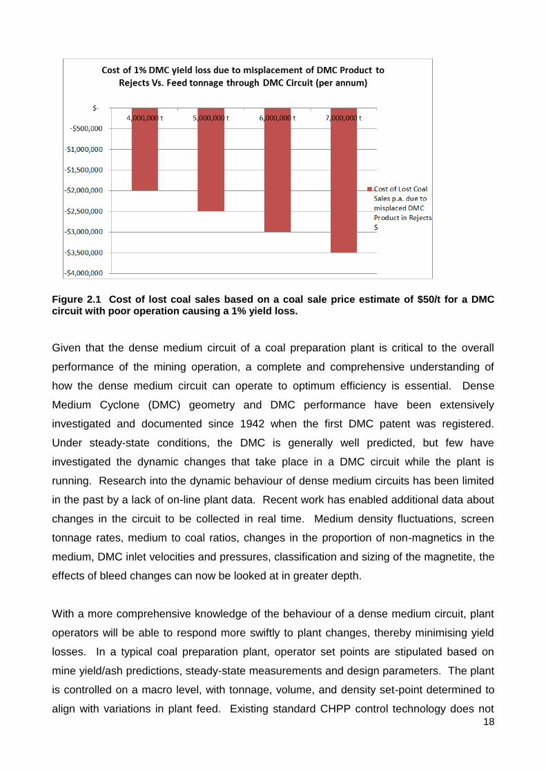
circuit would represent $3 million per year in lost sales. Figure 2.1 shows the potential lost

value in a Dense Medium Cyclone circuit through poor operation for a 10 million ROM

(Run of Mine) tonne per annum plant. The relative proportions of feed tonnes going to the

DMC circuit per annum and the cost of lost coal sales are compared. This is a simplistic

view and only considers lost sales due to misplaced tonnes to rejects. Consideration of

real value lost should also include the cost of mining, processing and storage of the

misplaced rejects.

18

Figure 2.1 Cost of lost coal sales based on a coal sale price estimate of $50/t for a DMC circuit with poor operation causing a 1% yield loss.

Given that the dense medium circuit of a coal preparation plant is critical to the overall

performance of the mining operation, a complete and comprehensive understanding of

how the dense medium circuit can operate to optimum efficiency is essential. Dense

Medium Cyclone (DMC) geometry and DMC performance have been extensively

investigated and documented since 1942 when the first DMC patent was registered.

Under steady-state conditions, the DMC is generally well predicted, but few have

investigated the dynamic changes that take place in a DMC circuit while the plant is

running. Research into the dynamic behaviour of dense medium circuits has been limited

in the past by a lack of on-line plant data. Recent work has enabled additional data about

changes in the circuit to be collected in real time. Medium density fluctuations, screen

tonnage rates, medium to coal ratios, changes in the proportion of non-magnetics in the

medium, DMC inlet velocities and pressures, classification and sizing of the magnetite, the

effects of bleed changes can now be looked at in greater depth.

With a more comprehensive knowledge of the behaviour of a dense medium circuit, plant

operators will be able to respond more swiftly to plant changes, thereby minimising yield

losses. In a typical coal preparation plant, operator set points are stipulated based on

mine yield/ash predictions, steady-state measurements and design parameters. The plant

is controlled on a macro level, with tonnage, volume, and density set-point determined to

align with variations in plant feed. Existing standard CHPP control technology does not

19

allow operators to see the subtle changes that occur in the dense medium, for example,

when the circuit is unstable. The measurement of non-magnetics in the medium has

shown some interesting relationships to DMC circuit stability, highlighting the need for a

thorough understanding of the medium changes that occur while the plant is in operation.

Better measurement, coupled with empirically derived models developed in past research

over the last 40 years, have enabled more accurate predictions to be used in a dynamic

model. It is important to note that the intention of this research was not to rework existing

empirical models, nor was it to develop new empirical models for DMC operation. Rather,

the purpose was to bring together the most useful and industry tested empirical models for

each unit operation and to establish a dynamic model for accurate plant prediction using

plant data for verification.

2.2 Separation Techniques

There have been numerous techniques employed over time to separate coal from its

surrounding mineral matter. Early coal sorting was done by hand and the use of water jigs

were employed. The modern Baum or ROM jig is still in use in some applications due to

its ability to remove stone effectively. Jig applications in Australia are becoming less

frequent due to the increase in size ranges treatable by DMC and also due to the relatively

high amount of near gravity material in Australian coals. Near gravity material is defined

as the material that lies within 0.02 relative density of the cut point, and the cut point refers

to the density fraction of coal in which approximately 50% of the coal will go to product and

50% to reject. This near gravity material can significantly affect the efficiency of the

separation equipment. When compared with water based processes, regardless of jig or

water washing cyclone type, the dense medium processes have been found to be superior

in separating the coal when there is a high presence of near gravity material. The use of

jigs are still considered practical in situations where a stone separation is made to the

feed, thereby releasing downstream capacity for additional processing loads, however the

prominence of jigs in the Australian coal industry is dwindling.

Historically the early dense medium processes in the coal industry used dense medium

baths as they allowed high throughput. As dense medium cyclones have become larger in

diameter, the need for separate top-size and mid-size processing has diminished. Baths

are also limited because Australian coals do not universally liberate well at a bath top size

of 100 millimetres. In many cases Australian coals liberate at or below 50 millimetre top

20

size. This is not the case for other coals such as those in North America where a higher

degree of liberation is possible at sizes over 100 millimetres. Ultimately it is the capital

cost, operational costs, coal characteristics and footprint that will determine the decision as

to which option to use. Nowadays, a DMC can process 100 millimetre top-sized particles

and can also process well below 10 millimetre top size efficiently, therefore eliminating the

need for an additional process to handle the mid-sized coals. There are still cases where

a bath is suitable and can upgrade a plant’s capacity at relatively low cost, however DMCs

have generally surpassed baths in Australia due to their versatility for a wide range of coal

types and size ranges. Furthermore, the use of centrifugal forces in a DMC increases the

sharpness of separation when compared to a bath for high near gravity situations. By far

the most dominant coarse coal processing equipment option utilised in Australia is the

dense medium cyclone as will be discussed later.

2.3 The Development of the Dense Medium Process

The principle of dense medium separation is based on fine grains in suspension in water

that behaves like a heavy fluid. In the presence of this heavy fluid called the “medium”,

material of lower density floats, and the material of higher density sinks. (Osborne, 1988)

Coal dense mediums are typically comprised of a suspension of magnetite, water, fine

coal and clays. The coal product floats as it is at a lower relative density compared to the

medium. Heavier rock and clay materials sink relative to the medium density. The

existence of significant amounts of near gravity material in a processing plant can lead to

misplacement of coal and rejects during the separation. While today, magnetite is widely

used as the main component of the medium for coal separation, this was not always the

case. Other fluids were previously trialled for early dense mediums.

In 1858, Henry Bessemer pioneered the first dense medium separator using metal chloride

salts in a cone shaped vessel. (Wood,1990, Davis,1987). One of the first separators to be

trialled in coal washing was the Chance cone in 1917, which used a slurry of sand and

water as the medium. (Scott, 1988) When in 1939, Dutch State Mines used a loess

suspension as a separating medium and utilised a hydrocyclone as a thickener for the

loess suspension, it was discovered that the overflow pipe occasionally blocked with

floating coal. Essentially the hydrocyclone was acting as a dense medium washer using

the loess suspension as the dense medium. (Davis, 1987) This led to the development of

the modern dense medium cyclone by Dutch State Mines.

21

The first dense medium baths that were developed used clay or loess as a medium

(Williamson and Davis, 2002). The disadvantage of utilising clay or loess, was similar to

the other organic liquids and metal salts previously tried. The difficulty and high cost of

medium regeneration prevented widespread adoption (Davis, 1987). Magnetite and

ferrosilicon were preferred due to their higher densities and strong magnetic recovery

advantages. It was not until 1922 that the first use of magnetite medium for coal cleaning

occurred on an experimental basis, and not until 1938 that magnetite was used

commercially as a medium. (Napier-Munn et al., 2013) It is here where a divergence

occurred between use of clays such as Loess and the use of magnetite and ferrosilicon.

The focus for Dutch State Mines in developing the dense medium was to find an easily

recoverable medium. Once magnetite and ferrosilicon came into widespread use, clays

were viewed as contamination and the emphasis was heavily placed on their removal

using magnetic separators. Recent research in to the role of non-magnetics in the

medium suggested that this insistence on contamination removal may have also had some

detrimental effects. This will be discussed later in Section 2.8.

The use of magnetite marked a key difference between dense medium applications in the

coal industry when compared with iron ore and diamonds. As the relative density and

composition of the dense medium required for coal was lower than for heavier minerals,

magnetite was able to be used in place of ferrosilicon. Coal dense medium processes

typically operate in the relative density range of 1.30 to 1.80. (Osborne 1988) Magnetite is

used as the dense medium and it has a density in the range of 4.2-5.1. The floats material

in the case for iron ore and diamonds is the reject as the density of the ore product is

higher than its surrounding in-situ mineral matter whereas the floats material for coal is the

product. For heavier minerals, ferrosilicon is used instead of magnetite when a higher

density range of operation is required, and sometimes a combination of the two are used.

Large diameter DMCs have permitted the use of coarser grades of media than in the past.

A reduction in the rate of loss of finer magnetite has been a major benefit, however, the

use of coarser grades is contingent on the DMC maintaining medium stability. At the lower

densities targeted for coal, the viscosity of the dense medium is rarely an issue in

Australia, though medium stability is significant. Other coal types, such as those in North

America may exhibit more frequent viscosity problems. While most coal plants are

22

designed to continually clean non-magnetics from the circuit, too little non-magnetic

material can also be detrimental to the stability of a circuit.

The early research in to the use of loess as a medium was abandoned due to the difficulty

of medium recovery, however, natural clay bands in the coal seam could be considered as

a potential medium stability enhancer in a dense medium cyclone or bath circuit in the

future. Recent research by Firth et al. (2011) has revealed that the presence of clays and

other fine non-magnetic material in the medium can be instrumental in determining its

stability. This is particularly the case when operating at a density target below 1.4RD

(Relative Density). This is currently an area of ongoing research. In the drive to maintain

high levels of production, and to rid coarse coal circuits of clay contamination, an

opportunity to acknowledge the benefits of the natural medium created by clays and fine

materials in the suspension of a cyclone may have been missed. This will be discussed

further in Section 2.8.

The effect of medium stability on the control of the dense medium cyclone circuit has been

an interesting subject of recent research. The New Acland coal mine in the Clarence

Moreton basin of South Queensland has provided some interesting data with numerous

instruments installed in the dense medium circuit. Coupled with regular sampling audits,

the CSIRO in conjunction with The University of Queensland have been collating data on

how a circuit responds to various changes, including the changing levels of non-magnetic

material in the medium. The outcome of this work will enable greater knowledge of circuit

behaviour and better control system design for faster response to stability issues in the

circuit.

The following sections will discuss the evolution of the dense medium cyclone, the role of

the medium and aspects of control of the dense medium cyclone circuit.

23

2.4 The Dense Medium Cyclone

In 1942, the first Dense Medium Cyclone was patented by Driessen, Krijgsman and

Leeman. Although the first design patent did not include a vortex finder, this feature was

added to the patent a few years later. (Wood, 1990) Dutch State Mines realised the

transferability of their invention to other minerals such as iron ore and diamonds, and in

1955 dense medium cyclones were first used in diamond processing (Napier-Munn,

Bosman and Holtham 2013). By 1960, there were twenty-three dense medium cyclones in

operation worldwide. (Wood, 1990) The modern DMC varies only slightly from the original

1960s designs by Stamicarbon. Some higher capacity designs have evolved, but many

manufacturers still adhere closely to the original DSM specifications (de Korte and

Engelbrecht 2007) The original handbook, entitled “The Heavy Medium Cyclone Washery

for Minerals and Coal” (Stamicarbon 1969) detailed key design parameters for the dense

medium circuit and is still referred to today. More recent additions have also been made to

the handbook, with the most recent being in 1994 (Cresswell, 2005). By 1980

approximately 370 DMC plants had been built and 270 of these were in the coal industry.

In Australia, by 1990, over 100 million tonnes of coal were processed by DMC (Wood,

1990) and today, the majority of wet processing coal plants in Australia use DMCs as a

key component.

Materials of construction such as alumina tile linings and ‘Ni-hard’ cast bodies have

improved dense medium cyclone component wear rates. Changed cyclone inlet designs

such as tangential, involute and scrolled evolute have advanced the flow patterns in the

DMC. Application of computational fluid dynamics has been used to improve flow patterns

and consequently wear rates for the redesigned inlets. In recent years, with the increased

use of DMCs in high volume commodities such as coal and iron ore, higher capacity and

larger diameter cyclones have emerged. Currently in the coal industry in Australia, the

largest DMCs in operation are 1500mm in diameter.

Although dense medium cyclones have existed since the 1940s, there have been only

minor adjustments to their design. Entry designs such as evolute entry have enabled

more consistent wear profiles when compared with the more traditional tangential entry

designs. The barrel and lower cone lengths have been varied from traditional DSM

designs in some cases to increase residence time in the cyclone, and higher capacity units

24

have also been developed. Essentially though, the structure and fundamental design of

the dense medium cyclone remains the same as it did 70 years ago.

Advances in dense medium processing have been more pronounced in the circuit design

area rather than in the DMC itself. The introduction of gravel pumps and variable speed

drives have improved the stability of operation, (Crowden, et al.,2013). Nucleonic gauges

and better tuning of process control loops have enhanced the control aspects of dense

medium processing. There have also been improvements to the magnetic separator

designs, (Cresswell 2005). Co-current separators have been replaced by counter-current,

and the strength of magnets has increased, thereby reducing the need for auxiliary

magnetic separators to do a second stage recovery. There are now new designs using

radial magnets and self-levelling magnetic separators. All of these advances have

enhanced the recovery of magnetite from the circuit while at the same time, efficiently

removing non-magnetics from the medium. Screening technology has also advanced with

the development of multi-slope screens (sometimes called “banana screens”) and static

“flume” screens. Screens are now larger with higher capacities, and screen panels have

also gone through various design improvements. Density tracers have also enabled better

monitoring of circuit performance without the need to wait several weeks for a result to be

returned from the laboratory, (Cresswell, 2005).

Despite worldwide improvements in dry sorting technology, dense medium cyclones

remain an efficient means of separating coal. Dry sorting technologies such as optical,

laser and X-Ray transmission sorting are unlikely to be widely adopted in Australia due to

their low capability for processing the high levels of near-gravity material normally present

in Australian coals. The presence of sticky clays that require desliming is also a limiting

factor. (Cresswell, 2005). It is likely that dry sorting technologies may be used as a pre-

treatment step at the front-end of a process to remove stone from the plant feed thereby

boosting overall CHPP capacity, however dense medium processes will remain integral in

future plant development.

The use of dense medium baths is less prevalent in Australia than overseas. In Australia,

approximately 11% of black coal (versus 20% overseas) is processed via dense medium

baths. (Kempnich, 2000) The presence of significant quantities of near-gravity coal and

the tendency of Australian coals to liberate at smaller top-sizes than in the USA, may be

the primary driver for this trend. As larger DMCs can now process at top-sizes of 100mm,

25

the need for dense medium baths has become less common in Australian new plant

designs, and plant upgrades often result in a switch to large DMCs.

Increases in cyclone diameter in recent years has prompted additional research into

cyclone efficiency. Original Dutch State Mines design parameters did not cater for larger

DMC sizes. The increased diameters have enabled treatment of coarser particles,

therefore generating higher throughput per unit. Larger DMCs have also in some cases,

eliminated efficiency drawbacks of running a biased Y-piece distributor adjoining two

DMCs in parallel. The introduction of gravel pumps that can handle larger top-size

particles has also played an enabling role in the evolution of larger DMCs. Clarkson and

Holtham (1998) noted that inefficiencies created by poor distribution of the slurry between

parallel modules can be equally as important as the intrinsic unit process efficiency. There

can also be efficiency losses associated with twin DMC pairs that are not geometrically

identical due to uneven wear, or different internal profiles. Where one DMC does not

operate at the same RD50 as its twin, misplaced coal will result. The author recalls one

such situation where a maintenance team thought that money could be saved by replacing

the single DMCs when individually worn instead of the entire DMC pair, with drastic

efficiency consequences. In plants where DMC maintenance is not tightly controlled with

metallurgical supervision, it is often preferable to replace twin DMCs with a single, larger

sized DMC, thereby eliminating the temptation to not replace the pair with identical twins,

and also eliminating the Y-piece bias effects. The benefits of better (lower) Eps for smaller

diameter DMCs are quickly negated if twin units operate at different cut-points. Larger

DMCs also allow easier entry for inspection and repair (Davidson, 2000).

26

Table 2.1: Typical cyclone dimension design trends compared with Dutch State Mines (DSM) original recommendations (De Korte and Engelbrecht, 2007)

Parameter DSM Recommendations Current Manufacturing Trends

Cyclone Diameter Up to 1500mm

Inlet Size 0.2 x cyclone diameter 0.2, 0.25 or 0.3 x cyclone diameter

Vortex Finder Diameter 0.43 x cyclone diameter 0.43 or 0.50 x cyclone diameter

Barrel Length 0.5 x cyclone diameter 0.5 to 2.5 x cyclone diameter

Spigot Diameter 0.3 x cyclone diameter 0.3 to 0.4 x cyclone diameter

Table 2.2: DMC Sizes. As dense medium cyclones increase in diameter, both capacity and top size increase, thereby providing opportunities for capacity expansion with fewer equipment items. Below dimensions are for Multotec cyclones. (de Korte and Engelbrecht 2007)

Standard-capacity Cyclones High-capacity Cyclones

Cyclone

diameter

Maximum

particle size

Coal Feed Maximum

particle size

Coal Feed

mm mm t/h mm t/h

510 34 54 51 99

610 41 81 61 145

660 44 97 66 175

710 47 114 71 207

800 53 149 80 270

900 60 196 94 355

1000 67 249 100 454

1150 77 351 115 638

1300 87 468 130 854

1450 97 608 145 1108

As cyclone diameter increases, centrifugal acceleration decreases, (Mengelers, 1982).

However, for coarser particles, the efficiency of a large diameter cyclone is equal or better

27

than that of a dense medium bath due to the presence of centrifugal acceleration which

creates increased g-forces inside the cyclone. The three product DMCs in use in coal

wash plants in China and South Africa are designed to utilise the ease of separation of a

large proportion of the feed in the inlet and first part of the DMC body to separate off a first

product, and diverting the middlings stream into a second cyclone-shaped chamber. This

early separation of coal in the inlet and entry to the DMC body is also observable in the

typical wear patterns of a DMC where considerable wear is present in the first revolution

after entry. Wear then reduces until the rejects reach the spigot where wear again

increases. The early removal of easily separated material allows more time for the near-

gravity material to separate without the increased particle interactions.

For finer sized particles, a breakaway size is thought to exist. Engelbrecht and Bosman

(1994) identified a potential drop in efficiency of minus 4mm particles in large cyclone

separators and a shift in cut density as cyclone diameter is increased (de Korte and

Engelbrecht 2007). Below the breakaway size, it is thought that efficiency deteriorates and

a shift in cut density will also occur (Crowden et al. 2013). Figure 2.2 demonstrates the

concept of breakaway size. De Korte and Engelbrecht (2007) noted that although a

breakaway size may exist, the perceived drop off in efficiency obtained in dense medium

cyclones is still much better than the efficiency of a water-based process such as a spiral

or teeter-bed separator (TBS).

Figure 2.2: Particle size versus imperfection for South African cyclones (mostly 610mm) suggesting that a breakaway size may exist. (de Korte and Engelbrecht 2007))

28

Anecdotally, there is considerable conjecture among Australian coal preparation experts,

as to whether the breakaway size issue really exists, or whether its appearance results

from sampling difficulties in plants. Finer coals can adhere to surfaces and not wash off at

the desliming screen, thereby being carried over into the coarse fraction. Sizing of screen

apertures can vary the bottom size of the coarse coal fraction, and misplaced coarse

material, particularly if flat in shape, can slip through screen apertures. The sample

treatment and analysis need to take into account the screen aperture size and possible

material misplacement of this size fraction. In addition to the potential for errors in

sampling around the screen cut point, Clarkson et al. (2002) found that over a series of

studies of larger DMC operations that processed particles larger than 1.0mm, no

significant degradation in performance (in terms of Ep) was found. Clarkson et al. also

found that there was no discernible difference in the +4mm and -4mm by 1mm size

fractions in terms of Ep performance. They suggested that other changes to plant

conditions and designs, such as operating at high medium to coal ratios to mitigate the

effects of high near gravity material could influence cyclone efficiency.

The presence of near gravity material can greatly influence the efficiency of separation of a

cyclone as shown in Figure 2.3 below.

Figure 2.3: Organic efficiency versus Ep for various percentages of near gravity material. (de Korte and Engelbrecht, 2007)

29

Clearly with higher proportions of near gravity material, determining the correct cut-point

(RD50) for the cyclone is critical to achieving the target yield and organic efficiency for a

particular coal.

As knowledge of dense medium cyclones and their efficiency parameters have evolved, so

have research and development of empirical models to describe DMC behaviour under

plant conditions. The following section outlines the most recent research into empirical

model development and also highlights some of the models that have been widely relied

upon in the coal industry for some time.

2.5 Empirical Models

Much of the previous work relating to dense medium cyclone modelling has been achieved

with steady state models based on empirical derivations. Wood et al. (1989), looked at

various aspects of dense medium cyclone operation from an empirical perspective. Past

experimental data and literature were utilized to develop a series of sub-models consisting

of empirically derived relationships between a number of measured parameters. (Figure

2.4) The eight sub-models in the Wood model considered medium behaviour as an

important parameter in predicting partitioning performance. The models also considered

unstable operation and factors influencing surging. 5mm tracers were used under “no

load” conditions to determine the partitioning performance without the presence of coal

feed or contamination in a pilot plant at the JKMRC (Wood, et al. 1989). The JKMRC

Wood Model has been widely used by coal industry practitioners as a predictor of DMC

performance. Under standard plant conditions, without surging or unusual events, and

with DSM Handbook design parameters for the cyclone, this model provides reasonable

predictions. As newer cyclone designs deviate from DSM standard designs, and

diameters increase beyond the limits provided by the experimental data used to derive the

Wood model, empirical model parameters may need to be modified.

30

Sub Description Symbol Value Units Sub Description Symbol Value Units Predicted Partition Curves sub-models 7 and 8, using Whiten partition curves

Model Model

No. FEED CHARACTERISTICS No. MEDIUM FLOWS per cyclone, if operating with medium alone Original - as in thesis

The Task SM2.1 medium split to u/f Quz/Qfz 0.101 - +4mm -4+2mm -2+1mm -1+0.5mm

circuit Feed rate (adb) 800 t/h SM2.2 underflow rate Quz 71 m³/h ρ50 1.298 1.321 1.352 1.414

product ash required 7.0 % SM2.3 overflow rate Qoz 632 m³/h Ep(75-25) 0.004 0.013 0.026 0.052

M:C in feed (minimum) 3.75 -

Washability Data - preliminary estimate MEDIUM FLOWS per cyclone, if operating with medium plus coal

feed coal density 1.45 RDU SM2.4 underflow rate (increases with sinks loading) Qum 86 m³/h

RD for target ash 1.36 RDU SM2.5 overflow rate Qom 537 m³/h

yield at target ash 62.0 % feed rate (also increases, improving M:C in feed) 623 m³/h

floats density at target ash 1.30 RDU SM2.6 medium split to u/f Qum/(Qum+Qom) 0.138 m³/h

Estimates of Flows of Feed Coal, Floats and Sinks

Mass Flows Check Point - medium-to-coal ratios

floats 496 tph feed recommended to be >4 4.5

sinks 304 tph overflow recommended to be > 3 5.6

Volume Flows underflow recommended to be > 2 2.0

feed coal 552 m³/h

floats 382 m³/h MAGNETITE SIZE and MEDIUM DENSITIES

sinks 170 m³/h Magnetite size intercept Prr 31.0 microns Modified - incorporating Pivot phenomenon, which has not been fully assessed against coal data

feed slurry for target M:C 2621 m³/h +4mm -4+2mm -2+1mm -1+0.5mm

Medium Densities in RD units ρ50 1.298 1.314 1.336 1.379

DMC SELECTION (DSM design) \ Do = 0.43 Dc and Di equiv is 0.20 Dc feed (prelim estimate) ρfm 1.21 Ep(75-25) 0.004 0.013 0.026 0.052

cyclone diameter Dc 1.000 m SM3 underflow ρum 1.642

vortex finder diameter Do 0.430 m Sm4 overflow ρom 1.143

spigot diameter Du 0.320 m differential (u/f - o/f) 0.249 (3)

inlet head (cyclone diameters) Head 9.0 Dc

inlet head (m of slurry) 9.0 m CUTPOINTS, RETENTION and VALUES OF Ep (75-25) in RD units

SM1 feed slurry flow Qf 704 m³/h SM5 Cutpoint for +4mm particles ρ50A 1.298 (2)

cyclones Required 3.73 (1) SM6 Retention Upper Limit (treat as indicator only) Rmax 1.389

Retention Range (treat as indicator only) 0.091 (4)

Decision Point(1) Round the number up to an integer commensurate with Check Point

preferred plant layout, or enter an alternative Dc. (2) Is the cutpoint where we want it? If not, adjust ρ fm to bring cutpoint

number of cyclones to be used 4 within 0.002 RDU of target.

For a single cyclone True Ep levels may be smaller than can be adequately resolved by float/sink techniques or even

SM1 feed coal solids Qfs 138 m³/h by tracers. They may or may not be as small as indicated here.

floats coal solids Qos 95 m³/h

sinks solids Qus 43 m³/h

(4) If retention range > 0.15 RDU and topsize >20mm there is danger of

surging with loss of yield. Take steps to reduce it.

(3) If differential > 0.4 RDU there may be retention which can progress to

surging and loss of yield.

0

25

50

75

100

1.2 1.4 1.6 1.8 2.0 2.2

% t

o R

ejec

t St

ream

RD

Wood Model - Partition Curves (Original)

+4mm

-4+2mm

-2+1mm

-1+0.5mm

0

25

50

75

100

1.2 1.4 1.6 1.8 2.0 2.2

% t

o R

ejec

t St

ream

RD

Wood Model - Partition Curves (with Pivot)

+4mm

-4+2mm

-2+1mm

-1+0.5mm

Figure 2.4a

31


Model Model
















feed coal 552 m³/h

























0

25

50

75

100

1.2 1.4 1.6 1.8 2.0 2.2

% t

o R

eje

ct S

tre

am

RD


+4mm

-4+2mm

-2+1mm

-1+0.5mm

0

25

50

75

100

1.2 1.4 1.6 1.8 2.0 2.2

% t

o R

eje

ct S

tre

am

RD


+4mm

-4+2mm

-2+1mm

-1+0.5mm

Figure 2.4b

32


Model Model
















feed coal 552 m³/h

























0

25

50

75

100

1.2 1.4 1.6 1.8 2.0 2.2

% t

o R

ejec

t St

ream

RD


+4mm

-4+2mm

-2+1mm

-1+0.5mm

0

25

50

75

100

1.2 1.4 1.6 1.8 2.0 2.2

% t

o R

ejec

t St

ream

RD


+4mm

-4+2mm

-2+1mm

-1+0.5mm

Figure 2.4c

Figure 2.4 (a, b and c): The JKMRC Wood model calculation spreadsheet with input parameters and calculated results. (Crowden et al., 2013) The model predicts the cut point, medium splits between underflow and overflow, flow rates, and a partition curve.

The Wood model was developed specifically for coal washing DMCs with diameters up to

710mm (Wood, 1990; Clarkson and Wood, 1991). The first equation in the Wood model

33

(Scott et al., 2013) uses cyclone dimensions and inlet pressure to predict the total

volumetric flow of medium and raw coal combined entering the DMC:

17.0

46.030.251087.2

o

ucf

D

DHeadDQ 1

where Dc, Du, Do are the cyclone, spigot and vortex finder diameters respectively in mm, and

Head is the inlet pressure in ‘diameters’. fQ is in the units m3hr-1

Once the volumetric flowrate of the feed is known, the second equation calculates the

fractional flow split of slurry (reject plus medium) to the spigot where Qu/Qf. This assumes

that there are low loadings of reject and Qu is the volumetric flowrate to underflow for

coarse rejects and medium combined in m3hr-1:

16.4

46.031.029.9

o

uc

f

u

D

DHeadD

Q

Q 2

This flow split is then used to predict the underflow medium density u in Equation 3:

CMDHead

Q

Qcf

f

uffu

f

:

5.011028.7 145.0562.034.1

]194.0[

3

)07.2(

3where f is the feed medium density, p is the medium grind size in microns (the

Rosin-Rammler intercept), and M:C is the volumetric feed medium to coal ratio. (Scott et al.,

2013)

34

With the medium split and underflow medium density now predicted, Equation 4 calculates

overflow density. The factor 1.52 in equation 4 below compensates for error in the flow

split equation due to cyclone head and sinks loading:

o f 1.52 f

f QuQ f

u

1QuQ f

4

The corrected cut point 50c for coarse particles (plus 4mm) is calculated using the feed,

overflow and underflow medium densities:

50c f 0.1250.154u 0.215o 5

If there is particle retention in the coarse fraction, then this is can be used to approximate

the minimum density of retention, Rmin. (Wood, 1990)

The sixth sub-model estimates the relative density range for retention of particles in the

cyclone. This relationship serves as a guide for cyclones with a feed topsize (dmax) of 0.04

to 0.05 times the cyclone diameter. Rmin is the minimum density of retention. (Wood,

1990)

PCM

HeadD

D

D

d

c

u

c

f 01.0:

2.0*02.0383.059.0 R- R minmax

6

Equation 7 predicts the separation density (cut point, 50d) and equation 8 the Ecart

Probable (Epd) for particles of any size:

50d 50c 0.06741

d1

10

7

Epd 0.033350cd 8

where d is the particle size (square mesh) in millimetres, and the factor 1/10 in equation 6

implies that the mean size of coarse particles is 10 mm.

35

Equation 8 generally predicts extremely low Eps for coarse particles, and is often

‘corrected’ by a factor to give values more in-line with those obtained experimentally

(Wood, 1990).

Once the 50 and Ep are determined, the modified Whiten equation (equation 9) is used to

generate a partition curve. The form of the equation means that a symmetrical S-shaped

curve is produced, with the high and low density tails constrained to give partition numbers

of 100 and 0 respectively. If DMC operating conditions are such that tails exist, eg coal lost

to reject, this model will not reflect actual DMC performance. (Scott et al, 2013)

PN 100

1 e1.0986

50

Ep

9

Figure 2.5 below demonstrates the process flow for the use of the Wood model.

36

Figure 2.5 Flow of model equations in the Wood Model. (Crowden et al. 2013, p145)

37

The JKMRC/Wood model (Wood et al. 1989) has proven to be a suitable predictor of DMC

behaviour under standard conditions, and is often used in practice due to its simplicity.

The model developed by Dunglison (1999) at the JKMRC also provides a good prediction

based on verification from experimental data, however, it is significantly more complex

than the Wood Model and was not widely published, thereby leading to its reduced use. It

does however, have broader application to iron ore, diamonds and larger dense medium

cyclones.

Dunglison (1999) extended the existing JKMRC models and developed a robust

quantitative mathematical DMC model which incorporated past work by Wood (1990), and

expanded it to include larger diameter cyclones greater than one metre. The Dunglison

Model also increased the applicability of the existing model by applying it to heavier

density applications such as diamonds. The model predicted the characteristic partition

curves, flow rates, medium splits and product densities. The Dunglison model utilised

elements of the Concha and Christiansen (1986) model and the pulp split model

developed by Schubert and Neese (1973). Its complexity is considerably higher than that

of the Wood model, though it is still readily implemented in an Excel spreadsheet or similar

software. Medium viscosity used in the Concha and Christiansen model, is considerably

more important in applications such as diamonds and iron ore where ferro-silicon medium

is used at higher densities, however for coal, viscosity is not normally an issue. Scott et al.

(2013) ran a side-by-side online comparison of the Wood and Dunglison models using one

hour of coal plant data and observed that the differences between the two models were

relatively minor. Ep comparisons were similar with the mean cut point over one hour

differing by 0.001 relative density point between the two models. While the Dunglison

model consistently predicted slightly lower overflow densities and slightly higher overflow

medium densities when compared with the Wood model, the cut point differences between

the Wood and Dunglison models were negligibly small. Experimental results from

sampling taken on the same day revealed that the predicted yield results aligned well with

the measured yields with a difference of 0.9%. Although this difference would be of

considerable significance over time, the other DMC predictions suggested that the

comparison was satisfactory. (Scott et al. 2013) In the case of the plant under study as

part of this PhD thesis, the benefit of online instrumentation measuring underflow and

overflow density over time has meant that this difference, however slight, in underflow and

overflow density model predictions can be ignored. In addition, the low focus on viscosity

negates the need for a more complex model. The author therefore recommends using the

38

Wood model, with its reduced complexity and direct applicability to coal applications, along

with online instrumentation measuring overflow and underflow density as part of the

dynamic model.

Prediction of separation density (RD50) and Efficiency (Ep) have also been investigated by

Hu and Firth (2010). They utilised measured medium densities of the feed, overflow and

underflow streams to predict RD50 and Ep without the need for float sink analysis. A

modified suspension-partition model was used to derive the following three equations to

describe medium density and RD50 for a conventional DMC.

9

10

11

Where Hm is the middle point of the effective separation region for the medium;

Ht is the DMC radius;

ρm is the density of the medium which is a linear function of the radial distance from the

wall, y;

ρf is the medium density of the feed;

ρo is the medium density of the overflow;

ρu is the medium density of the underflow;

and RD50c is the separation cut point.

The Partition number, PN is given by Equation 12:

12

Where αc,S and αc,H are the mean values of αc (the volume fraction of particles) in the

ranges of HS and Ht’ respectively and where HS and Ht’ are parameters in the suspension-

partition model. (Ht’ is the radius of the DMC and Hs is the particle separation boundary).

39

They found that these models generally fitted the partition curves for the plant data used,

with close agreement with the tracer test results. It was determined that the results

showed a sufficiently close indication for use in on-line monitoring. A comparison of

accuracy of the Hu and Firth (2010) model and the Wood model has not been made here,

however it appears that either model would work for the purpose of the dynamic model for

typical Australian coals provided that the DMC is of conventional design. If the DMC were

to deviate from DSM design geometry conventions, it would be necessary to modify the

equations.

Desliming Screen Models

Various other models are useful in determining a dynamic model of a coal dense medium

circuit. Desliming screen designs follow various rules of thumb outlined in the DSM

Handbook and as specified by McKay (1984), and drainage capacities for multi-slope

screens were experimentally determined in ACARP report C7048 (Crowden et al. 2013).

Table 2.3 represents the best estimates of drainage rates for multi-slope de-sliming

screens based on this research.

Table 2.3: Recommended drainage capacities for multislope screens

From Crowden et al. (2013, p52) Nine modules from six plants were studied as part of ACARP study C7048 and screen apertures from 0.5mm to 1.4mm wedge wire were considered.

Aperture mm (wedge wire) Drainage m3/h/m2

0.5 20

1.0 65

1.4 80

Screen loadings are generally determined using the DSM Handbook formula as follows:

13

Where C is t/h per m width, da is average grain size in mm, and pr is the RD of an average

particle

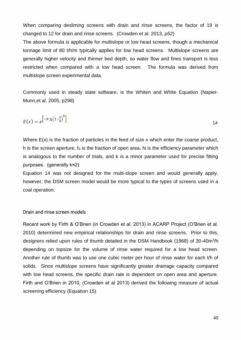
40

When comparing desliming screens with drain and rinse screens, the factor of 19 is

changed to 12 for drain and rinse screens. (Crowden et al. 2013, p52)

The above formula is applicable for multislope or low head screens, though a mechanical

tonnage limit of 80 t/h/m typically applies for low head screens. Multislope screens are

generally higher velocity and thinner bed depth, so water flow and fines transport is less

restricted when compared with a low head screen. The formula was derived from

multislope screen experimental data.

Commonly used in steady state software, is the Whiten and White Equation (Napier-

Munn,et al. 2005, p298)

14

Where E(x) is the fraction of particles in the feed of size x which enter the coarse product,

h is the screen aperture, f0 is the fraction of open area, N is the efficiency parameter which

is analogous to the number of trials, and k is a minor parameter used for precise fitting

purposes. (generally k≈2)

Equation 14 was not designed for the multi-slope screen and would generally apply,

however, the DSM screen model would be more typical to the types of screens used in a

coal operation.

Drain and rinse screen models

Recent work by Firth & O’Brien (in Crowden et al. 2013) in ACARP Project (O’Brien et al.

2010) determined new empirical relationships for drain and rinse screens. Prior to this,

designers relied upon rules of thumb detailed in the DSM Handbook (1968) of 30-40m3/h

depending on topsize for the volume of rinse water required for a low head screen.

Another rule of thumb was to use one cubic meter per hour of rinse water for each t/h of

solids. Since multislope screens have significantly greater drainage capacity compared

with low head screens, the specific drain rate is dependent on open area and aperture.

Firth and O’Brien in 2010, (Crowden et al 2013) derived the following measure of actual

screening efficiency (Equation 15)

41

15

Where Pa is the partition number for actual screening efficiency, Rf is the proportion of

water originally in the feed that reports to the oversize flow stream, and Ap is the screen

aperture for N attempts of a particle passing through the screen. represents particle size

Specific Drain Rate was determined from a study in 2000 by Meyers et al. where a strong

relationship between solids drain rate and volume drain was found. The key relationship

identified was that the main factor influencing transport through the particle bed was

hydraulic, and not stratification. From this, the specific drain rate formula (O’Brien et al.

2002) was derived in equation 16.

16

Where SDR is the specific drain rate (m3/h/m2), C1 and C2 are constants, Q is the

volumetric flow rate of the medium or water and underflow solids per m2 of screen, Ap is

the screen aperture width (mm), OA is the Open Area fraction, and ThiC is the volume

fraction of coarse coal in the feed. (Crowden et al. 2013)

From the specific drain rate equation, the relative medium drain rate (RMDR) is

determined by dividing the equation by the volumetric flow rate of the medium or water and

underflow solids per square metre of screen. Firth and O’Brien 2010 showed that Rf for

the drain section could be described by another relationship which gives an estimate of the

final drain section moisture level given that the drain rate is reasonable.

17

As a rule of thumb, it is generally assumed that the rinse section final moisture level is

around 20% by mass of the oversize stream. (Crowden et al. 2013)

Magnetic Separator Models

Numerous models have been developed to describe the dilute circuit of a dense medium

plant. Often a figure of 99.8% recovery of magnetite is quoted for modern magnetic

separators. This is usually based on the level of magnetite loss in the tailings stream.

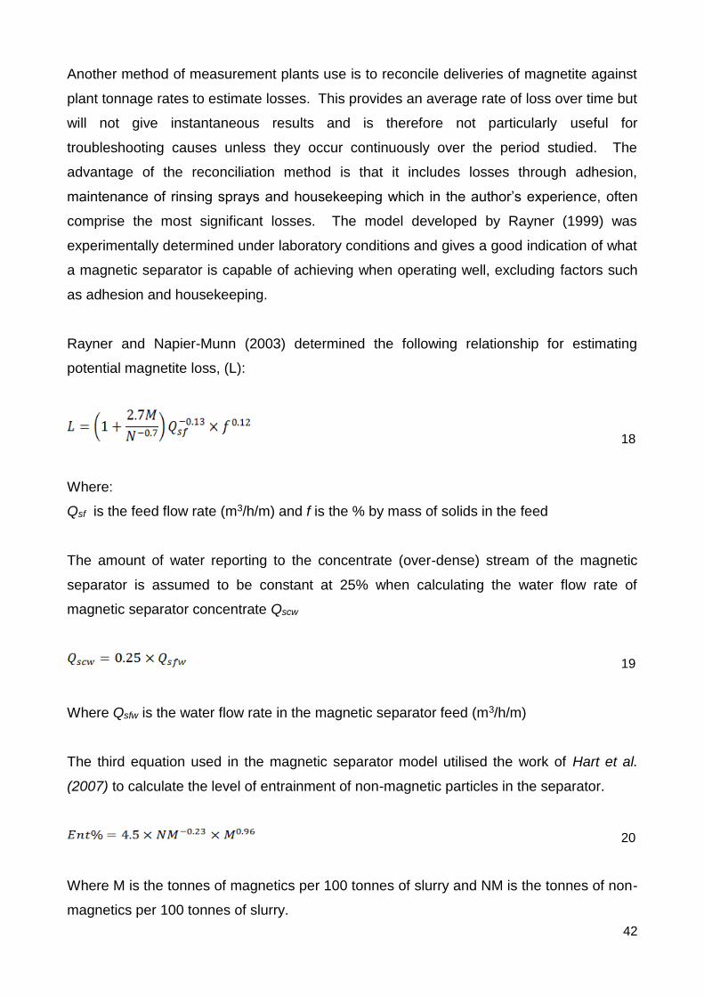
42

Another method of measurement plants use is to reconcile deliveries of magnetite against

plant tonnage rates to estimate losses. This provides an average rate of loss over time but

will not give instantaneous results and is therefore not particularly useful for

troubleshooting causes unless they occur continuously over the period studied. The

advantage of the reconciliation method is that it includes losses through adhesion,

maintenance of rinsing sprays and housekeeping which in the author’s experience, often

comprise the most significant losses. The model developed by Rayner (1999) was

experimentally determined under laboratory conditions and gives a good indication of what

a magnetic separator is capable of achieving when operating well, excluding factors such

as adhesion and housekeeping.

Rayner and Napier-Munn (2003) determined the following relationship for estimating

potential magnetite loss, (L):

18

Where:

Qsf is the feed flow rate (m3/h/m) and f is the % by mass of solids in the feed

The amount of water reporting to the concentrate (over-dense) stream of the magnetic

separator is assumed to be constant at 25% when calculating the water flow rate of

magnetic separator concentrate Qscw

19

Where Qsfw is the water flow rate in the magnetic separator feed (m3/h/m)

The third equation used in the magnetic separator model utilised the work of Hart et al.

(2007) to calculate the level of entrainment of non-magnetic particles in the separator.

20

Where M is the tonnes of magnetics per 100 tonnes of slurry and NM is the tonnes of non-

magnetics per 100 tonnes of slurry.

43

The equations described in this section assisted in determining balances around the unit

operations in the dynamic model. They were used in conjunction with the material balance

and washability data to determine the performance of the circuit. The critical distinction

between this and prior work was that the breakdown of components into non-magnetics,

magnetics, coal and water has not been fully explored previously. The influence of the

level of non-magnetics on the circuit over time with various perturbations has not

previously been dynamically modelled, and the availability of new instruments enabled

better circuit measurement.

2.6 Practical Application of DMC Models

Practical realities of coal processing plants introduce additional variation due to imperfect

maintenance practices, lack of comprehensive information, variations in operator

practices, varying levels of medium contamination, seam and working section variation,

regularity of feed-off events (stoppages), continuous variation in feed quality and the

degree of high near gravity material present. In this environment it is difficult to develop

empirical models that hold over a range of operating conditions.

Under plant conditions, dynamics can play a significant part in the final efficiency

outcomes. Yields and recovery are often affected by dilution, weightometer error, varying

size distributions and circuit loadings. The influence of medium contamination on coarse

coal DMC circuit efficiencies and throughput has been partially explored by O’Brien et al.

(2013), and Firth et al. (2013) and research is ongoing. Differing manual operator input

decisions made at the time of production can also influence yields, often without the cause

of the yield change being visible to the operator from the control panel. Ongoing

monitoring of plant conditions using on-line or real-time data provides an opportunity to

present the realities of plant dynamics and overlay the prediction of theoretical DMC

models to use as a guide to where plants may be deviating from ideal operation.

Where plants operate under relatively standard, stable conditions, the Wood Model

provides a simplistic yet reasonably accurate guide to the efficiency of a plant. Coupled

with density tracer tests, plant metallurgists can obtain a virtually instantaneous indicator of

their plant efficiency on any particular day. Dynamic measurements of DMC underflow

and overflow medium densities provide a useful comparison and a guide to the stability of

44

the circuit. More difficult is the measurement of medium to coal ratios. In general, CHPP

instrumentation such as feed weightometers are not sufficient to provide an accurate

measure if consideration is given to the constant variation in raw coal sizing, and the

coarse versus fines circuit split at the desliming screen. However, CSIRO equipment is

available and can be retrofitted onto a screen to analyse screen motion and measure

mass flow across the screens. Provided that it has been calibrated, this gives a more

accurate measure of screen yields and therefore coal flowrates. The medium flowrates

can be estimated based on pump curves and using the density gauge also as a guide.

Analysis of online results showing differential and offset pose an interesting challenge.

Often it is assumed that plant conditions are relatively stable once a plant has been

operating on a particular seam for some time. In practice, the concentration of non-

magnetic material in the circulating medium can raise or lower depending on bleed rates

and momentary feed-off events. The offset, which is commonly assumed to be constant

when making calculations around a DMC circuit, can change, and the relative density can

vary considerably from the cut point despite the nucleonic gauge indicating that no change

has occurred. Recent research by Firth et al. (2014) has indicated that the prediction of

differential by measurement of overflow and underflow densities is linked with stability of

the circuit. Where the level of non-magnetics in the medium drops to a relatively low level,

the traditional plant indicator of nucleonic density lacks the ability to show this instability.

In their work, Firth et al. (2014) observed that the underflow density behaved differently to

the overflow density over time leading to an observed higher differential and consequent

circuit instability. Figure 2.6 below showed a typical Australian coal DMC circuit operating

in a low density range of 1.32-1.42. It can be observed from this figure that following an

increase in the density set point by the plant operator, the circuit became unstable and the

underflow density RhoU rose while the nucleonic density gauge (RhoFN) remained steady.

Figure 2.7 demonstrates the same example with the differential and offset moving when

the underflow density rises.

45

Figure 2.6: (after Firth et al. 2014, p150) Observation of underflow density RhoU, Overflow density RhoO, Feed medium density RhoFN and the calculated cut point estimate RD50est following a density change from 1.32 to 1.4.

Figure 2.7: (after Firth et al. 2014, p151) Differential measured for the situation described in the previous figure. Offset can also be seen to move by 0.04 RD upwards.

46

An explanation for the circuit instability observed is proposed below.

Figure 2.8: after Firth et al. (2014) Increase in feed medium density in a low relative density range.

Corresponding underflow density becomes unstable when a rapid density change upwards is coupled with an increased bleed of medium to the dilute circuit. The correct medium sump level is controlled by the operator via a bleed valve to transfer correct medium to the dilute circuit. Water additions to the correct medium sump are automatically controlled via a feedback loop to the nucleonic density gauge (RhoFN).

A density change upwards occurred at approximately 11:00hrs. (Figure 2.8) This

corresponded with an increase in the level of bleed to the dilute circuit to reduce the sump

47

volume. The bleeding to the dilute would have caused a change to the level of non-

magnetics in the circuit and as the circuit was operated at a relatively low density (1.32-

1.4), the underflow density began to rise markedly in comparison with the overflow density.

The cut point estimate (RD50est) which was calculated, was also seen to rise slightly as

the underflow density increased. This was despite the nucleonic gauge density (RhoFN)

remaining steady during this time. The calculated differential rose to 0.55 which is outside

the range for stable operation and indicated the potential for retention and surging in the

DMC.

Figure 2.9 on the following page is an example of a coal DMC circuit where the feed

medium density was decreased at 14:00 hours, by 0.04RD. The underflow medium

density increased due to an overflowing correct medium sump level. The overflowing

sump acted as a bleed to the dilute circuit, thereby losing non-magnetics. The increase in

underflow density changed the differential to 0.4. While the nucleonic gauge (RhoFN) was

steady at 1.34RD, the estimated cut point (RD50est) moved upwards from 1.40RD to

1.44RD. This situation could have significant yield implications for a coal washery.

48

Figure 2.9: after Firth et al. (2014,p159) The effect on DMC circuit with a feed medium density decreased at 14:00hrs from 1.38RD to 1.34RD.

Estimated separation density remained unchanged and not 0.04RD below due to an increase in underflow density and consequently differential.

2.7 Density Tracers

One of the most effective tools developed to assist plant process engineers to assess their

circuit efficiency on any given day is the density tracer. These simple, typically cube

shaped, plastic resin particles cover a range of densities and allow a partition curve to be

49

generated, thereby giving a relatively instantaneous indication of dense medium circuit

health. The use of density tracers as an alternative to traditional float sink analysis (ISO

Standard 7936:1992 Hard coal – Determination and presentation of float and sink

characteristics) provides a cost effective and fast turnaround solution of determination of

cyclone efficiency. Davis (1987), used specially prepared 5 millimetre density tracers in a

200mm gravity fed cyclone to monitor a magnetite medium and medium viscosity under

pilot plant conditions to assess DMC efficiency at two different densities and two spigot

sizes. He measured the viscosity continuously using an on-line viscometer and used

varying amounts of montmorillonite clay addition. This research did not investigate relative

densities below 1.4, and only high swelling clays were considered. More will be discussed

regarding viscosity effects in Section 2.8 - The Medium.

Recent advances by the Council for Science and Industrial Research (CSIR) in South

Africa and collaborative work by Wood (2012), and Virginia Tech and also a separate

study have developed the use of transponder technology for online monitoring of density

separation efficiency (Wood et al. 2014). Radio frequency Identification (RFID) density

tracers were developed to measure DMC efficiency with fewer people required to

administer the test (Honaker, et al. 2007). RFID tracer technology was utilized as part of

the research discussed here and is outlined under the Experimental Work section of this

thesis. The purpose of RFID Tracer use for this research was to determine residence

times in and transfer times between vessels within the plant. Tracers are a consumable

item and are relatively low in cost when compared with float-sink alternatives. Residence

times of coarse particles in vessels have been previously achieved using the smart rock

technology developed by the CSIRO in a previous ACARP Project. The requirement to

recover 100% of the smart rocks however, is considered too difficult to practically achieve

in the plant. Smart rocks are by comparison, more expensive to replace than the radio

frequency tracer technology. The company Metso has also developed an RFID tracer

product which can trace coal particles from the mine to the port. These blast and crusher

resistant tracers are comprised of only one density (approximately 1.3), however they

serve a useful purpose in tracking mining batches through the processing plant to the port.

50

2.8 The Medium

Medium Composition

The medium is a slurry mixture of magnetite, water, fine coal and clays. Ideally a medium

should be stable but of relatively low viscosity (Rayner, 1999). At high densities, viscosity

can be a problem, however at low densities, some level of stabilisation of the medium

prevents coarser solids from settling out from the dense medium. In the case of low

stability of a dense medium, and particularly where high near gravity coal also exists, there

is a tendency for retention to occur in the cyclone and the magnetite to classify in the

dense medium cyclone. If a high differential exists between overflow and underflow

densities of the medium, then surging can occur. (Crowden et al. 2011)

Medium stability and the efficiency of clay removal at New Acland CHPP has been the

subject of further investigation by Firth et al. (2011), O’Brien et al. (2008) and O’Brien et al,

(2013). Firth et al. (2011) found that the major factors influencing the settling behaviour of

the medium were the volume fraction of non-magnetic material and the mean size of the

magnetic particles.

Further definition of the medium has been developed with respect to size distribution. It

was found that the constituents of the medium are as follows (Firth et al, 2011):

clay with a nominal size of about 0.010mm

magnetite with a nominal size of 0.040mm

fine coal with a nominal size of 0.080mm, and

small coal with a nominal size of 0.450mm.

Firth et al. (2011) also determined that for the sites studied, medium stability became more

significant for plants operating at relative densities below 1.4. They concluded that small

coal was not considered to be part of the medium while fine coal was. It was considered

that material below 200 microns could be considered to be part of the medium while

particles greater than 200 microns were not. (Firth et al. 2011) Material that is part of the

medium is significant in terms of influencing medium stability, while material that is not part

of the medium will affect overall medium density but not greatly influence medium stability.

51

Medium viscosity and stability

For many dense medium plants, removal of contamination (non-magnetics) in the medium

is critical because the clays can accumulate in the circuits. This is a known problem with

dense medium circuit performance and is important in diamonds, iron ore, and other high

density dense medium applications. The primary reasoning behind removal of non-

magnetic contamination in dense medium circuits is related to viscosity. Iron ore,

diamonds and other high density applications of dense medium circuits suffer from

excessive viscosity related to the presence of clays and other contamination in the

medium. (Napier-Munn and Scott, 1990) Figure 2.10 demonstrates the difference in

apparent viscosity at higher densities when comparing fresh medium with contaminated

medium.

Figure 2.10: The difference in apparent viscosity when medium is contaminated versus fresh medium for a diamond operation. (Rayner 1999)

The densities used in the graph were for much higher densities than for those used in coal. It not clear from this data whether the relationship still holds for coal densities, however a flattening of the apparent viscosity line at lower densities is visible on this graph.

The inclusion of a demagnetising coil in these cases was found to be beneficial in reducing

viscosity, however, in Australian coal plants, the presence of demagnetising coils to

remove magnetic flocculation is extremely rare. Napier-Munn and Scott also listed

medium density, solids density, particle size distribution, particle shape and fine

contamination as other factors influencing medium viscosity. Viscosity is also sensitive to

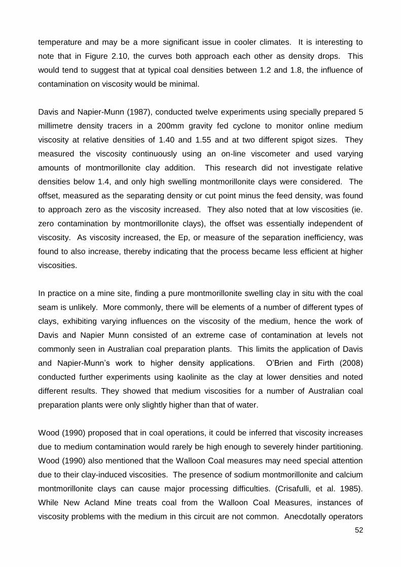
52

temperature and may be a more significant issue in cooler climates. It is interesting to

note that in Figure 2.10, the curves both approach each other as density drops. This

would tend to suggest that at typical coal densities between 1.2 and 1.8, the influence of

contamination on viscosity would be minimal.

Davis and Napier-Munn (1987), conducted twelve experiments using specially prepared 5

millimetre density tracers in a 200mm gravity fed cyclone to monitor online medium

viscosity at relative densities of 1.40 and 1.55 and at two different spigot sizes. They

measured the viscosity continuously using an on-line viscometer and used varying

amounts of montmorillonite clay addition. This research did not investigate relative

densities below 1.4, and only high swelling montmorillonite clays were considered. The

offset, measured as the separating density or cut point minus the feed density, was found

to approach zero as the viscosity increased. They also noted that at low viscosities (ie.

zero contamination by montmorillonite clays), the offset was essentially independent of

viscosity. As viscosity increased, the Ep, or measure of the separation inefficiency, was

found to also increase, thereby indicating that the process became less efficient at higher

viscosities.

In practice on a mine site, finding a pure montmorillonite swelling clay in situ with the coal

seam is unlikely. More commonly, there will be elements of a number of different types of

clays, exhibiting varying influences on the viscosity of the medium, hence the work of

Davis and Napier Munn consisted of an extreme case of contamination at levels not

commonly seen in Australian coal preparation plants. This limits the application of Davis

and Napier-Munn’s work to higher density applications. O’Brien and Firth (2008)

conducted further experiments using kaolinite as the clay at lower densities and noted

different results. They showed that medium viscosities for a number of Australian coal

preparation plants were only slightly higher than that of water.

Wood (1990) proposed that in coal operations, it could be inferred that viscosity increases

due to medium contamination would rarely be high enough to severely hinder partitioning.

Wood (1990) also mentioned that the Walloon Coal measures may need special attention

due to their clay-induced viscosities. The presence of sodium montmorillonite and calcium

montmorillonite clays can cause major processing difficulties. (Crisafulli, et al. 1985).

While New Acland Mine treats coal from the Walloon Coal Measures, instances of

viscosity problems with the medium in this circuit are not common. Anecdotally operators

53

have indicated that at high density set-points, above 1.6RD, they sometimes experience

blockages in the plant rejects system, however this may not necessarily be due to the

proportion of non-magnetics in the medium. The plant has been designed to efficiently

strip out non-magnetic contamination material from the dense medium circuit to avoid a

recirculating clay load within the plant. It appears that the recommendations made by

Crisafulli et al. 1985, of direct feeding, adding water at the feeder breaker to move clays

beyond the ‘sticky’ region, and minimising raw coal storage, have been followed in this

plant design. Through the work of O’Brien et al. (2013) on New Acland medium samples,

it has been demonstrated that the plant non-magnetics levels are generally low. This

could mean that the magnetic separators are over-compensating by removing too much of

the stabilising contamination in the medium. Davis and Napier-Munn (1987) did note that

in coal washing in which the volume solids concentration of feed medium was relatively

low, typically 7-18%, classification of the medium in the cyclone played a predominant role

in determining the product medium density whereas for diamonds and other higher density

operations, sedimentation was the major factor.

Viscosity is an interesting point of contrast between the work of these researchers. The

narrow range of tests applied, the different clays selected, and comparison with real plant

situations provide some insight into why these differences exist. It appears that there are

instances where viscosity can play a part in coal washing, however, instances are not

widely acknowledged and certainly not widely measured in plant operations. Extreme

cases occasionally present to a plant, however, often processing difficulties are attributed

to other causes such as blocked chutes, or sticky clays without consideration of the minute

by minute differences in efficiency that could potentially be caused by viscosity effects.

For the purposes of modelling the coal plant at New Acland, the Wood model is the most

appropriate choice, however the Dunglison model could be applied in future dynamic

models for coal and other minerals if more online viscosity information were to become

available.

Medium rheology, stability and viscosity have been extensively explored by Davis and

Napier Munn (1987) and also by He and Laskowski (1993). The former identified a

reduction in efficiency with increasing clay contamination due to medium rheology. He and

Laskowski highlighted the influence of stability, separation cut-point and differential and

investigated the effects of different particle sizes on medium properties. The density

differential between the cyclone underflow and overflow is thought to characterise medium

54

stability. He and Laskowski (1993) tested a number of grades of magnetite and found that

for the same medium density, the density differential was higher for coarser grades of

magnetite. In coal applications, typical DSM guidelines are for finer magnetite to be used

in lower density applications and coarser grades in higher density applications.

In day to day operations, the importance of the medium is often overlooked. Plants are

given tools to manage density, pressures and levels, however, the medium composition is

not a visible measure and can therefore be easily ignored. Despite the importance of

relative proportions of non-magnetics in the medium, online measurement has not been

available to plant operators and metallurgists in the past. Plant operators have relied upon

other metrics such as density and DMC pressure to give indications of how the circuit is

performing without visual indication of the density differential. When the density differential

exceeds 0.4, DMC surging is more likely to occur (Crowden et al, 2013) Evidence of

surging in the presence of very low percent non-magnetics has not been measured except

on reject weightometers which are notoriously high in error (commonly +2%) and may not

be able to distinguish a surging event against the background of plant noise. In some

cases, DMC surges can be observed visually on the primary reject drain and rinse

screens. Apart from visual inspections, surging DMCs are difficult to detect unless they

drastically affect the product quality readings. Product and reject weightometers can be

affected by surging centrifuges which may mask or confuse the issue. Similarly, variations

in feed from one haul truck to the next can generate fluctuations on weightometers that

resemble surging. With new instrumentation at the New Acland plant, surges have been

detectable by use of accelerometers on the product and reject drain and rinse screens as

well as by observation of the density differential between drain and rinse screen under-

pans for product and reject screens.

Medium Recovery and stability

Recovery of medium in a coal DMC circuit can be critical to plant profitability. Large losses

of magnetite are costly and considerable efforts are employed by plant metallurgists to

stem losses of magnetite through the various possible sources. Masinja (1992) identified

sources of medium losses in dense medium plants, and in particular, developed an

empirical model for adhesion losses – where medium adheres to the coal or ore on the

screens. Considerable losses of magnetite were also noted by Masinja (1992) in coal

plants where a high rate of stoppages occurred. Given that an appropriately sized, well

55

designed and maintained modern magnetic separator is over 99.8% efficient, (Norrgran,

2010) the recovery of magnetite is less important in relation to the focus of this study. In

the author’s experience, for a magnetic separator that is properly installed and maintained,

much of the magnetite losses can be attributed to housekeeping, floor sump overflows,

and poor operation of drain and rinse screen sprays.

Rayner (1999) developed an empirical model for magnetic separators, however, non-

magnetic contamination was included as a percentage of feed solids. He recommended

further work that considered the influence of different size distributions of non-magnetics.

Rayner noted that it was the finest solids which most greatly influenced the rheology of the

medium. Dunglison (1999) also noted that the concentration of solids influences the

rheology of the medium. Likely sources of the fine solids are from recirculating loads, coal

breakage and de-slimed coal and mineral matter present in the feed that carry over into

the coarse circuit.

Stabilising the medium

In addition to finer magnetite, the clays and fine coal present in the medium are also

stability enhancers. Too much medium contamination by non-magnetics can occur in iron

ore and diamonds processing leading to high viscosity in the medium. This has generated

a widespread fear of viscosity causing damaging ramifications for processing in coal

applications. Whereas in iron ore and diamonds DMC operations removal of

contamination is done to reduce viscosity, in Australian coals, viscosity is significantly less

important. There are, of course, exceptions, and in the case of bentonite clay types, the

high swelling characteristics can induce viscosity effects at very low concentrations. In

some coal plants on certain seams, this can be a reason to bleed more medium to the

dilute circuit. It is, however, possible to go too far. Circuits can lose stability by bleeding

excessive amounts of non-magnetics from the system via the dilute circuit and plants then

compensate for this by adding finer magnetite. This results in higher operating costs.

It is commonplace in Australian coal plants to select a finer grade of magnetite to combat

instability problems in a circuit. The difficulty of using finer magnetite is that the highest

losses of magnetite often occur in the finer size ranges. This was confirmed by Davis and

Lyman (1983) who showed that magnetite losses in separator tailings were finer than in

the feed when new magnetite was used in the circuit, and when very dilute feeds were

56

presented to the magnetic separator. Consequently, a plant may invest in finer magnetite

only to have it rapidly lost due to overflowing sumps, surface adhesion on rinse screens,

inadequate coal rinsing, poor housekeeping, or surging volumes in the magnetic

separator.

Medium samples are thought to vary in size distribution according to fresh feed additions

of magnetite, however, analysis of some magnetite samples from New Acland coal

preparation plant by O’Brien and Taylor (2013) revealed that the sizing of the magnetite in

the correct medium remained largely the same regardless of new magnetite additions.

This is shown in Figures 2.11, 2.12 and 2.13 below.

Figure 2.11: Correct medium magnetite samples from New Acland analysed using a Malvern laser particle sizer. Size distribution fractions for the various samples

Individual samples show very high correlation. (O’Brien and Taylor, 2013).

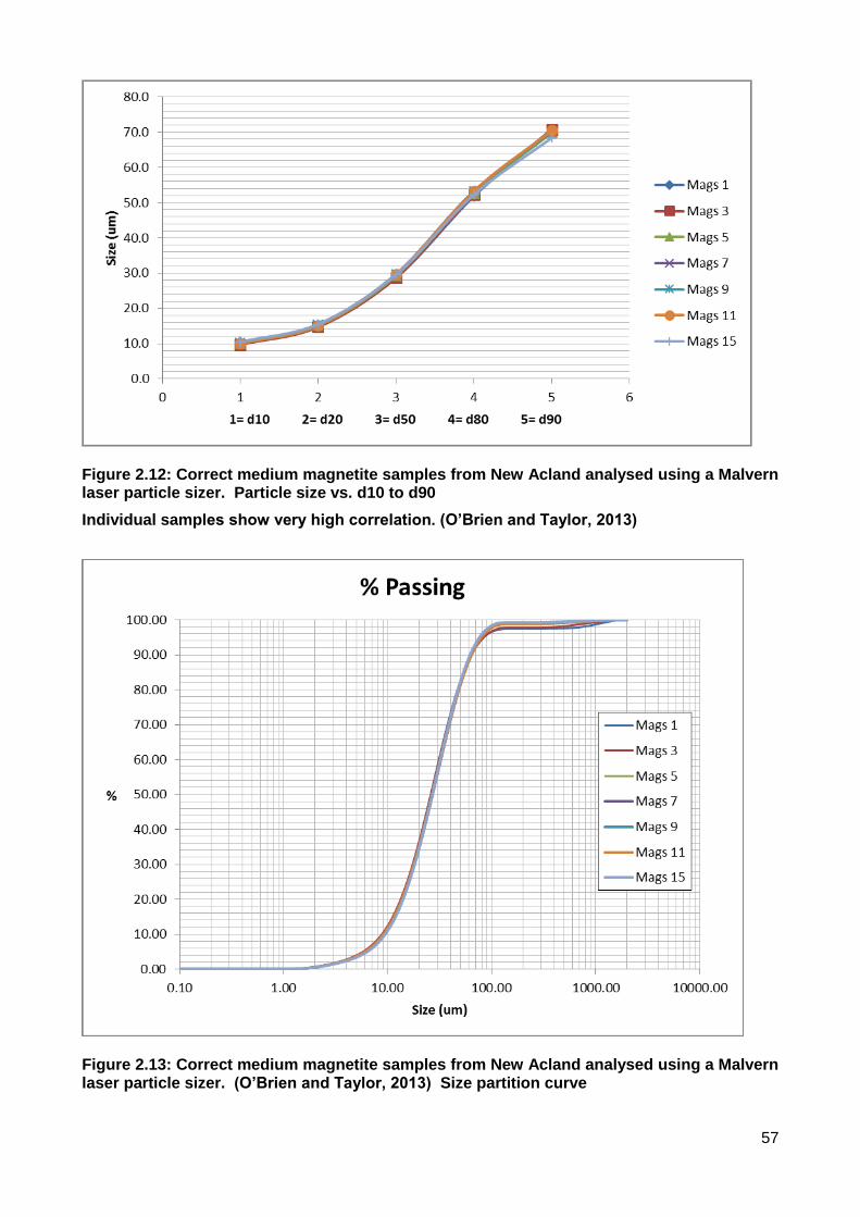
57

Figure 2.12: Correct medium magnetite samples from New Acland analysed using a Malvern laser particle sizer. Particle size vs. d10 to d90

Individual samples show very high correlation. (O’Brien and Taylor, 2013)

Figure 2.13: Correct medium magnetite samples from New Acland analysed using a Malvern laser particle sizer. (O’Brien and Taylor, 2013) Size partition curve

58

A possible reason suggested for the lack of variation in magnetite sizing was that there

could have been an immediate loss of non-magnetics and finer magnetite particles within

the first revolution through the magnetic separators and therefore, the finer magnetite

additions may not be generating the expected stability in the circuit. (O’Brien,et al. 2013)

It is proposed that while expensive finer magnetite has the effect of stabilising a medium,

the same effect may be available from the free clays which are so efficiently removed from

the system by the magnetic separators. Plants could potentially utilise natural clays

inherent in the raw coal feed to enhance DMC circuit operation to create a similar effect to

the traditional use of Loess as a medium. In this case, however, recovery of the clays

would not be an issue because the feed would continually refresh non-magnetic material

into the circuit. Maintaining and controlling the level of non-magnetics in a circuit when

targeting low density cut points may generate the same stability benefits at significantly

lower cost. Achieving this in practice however, may be more difficult. Non-magnetics are

currently not measured on an on-line basis although work in this area is progressing.

Level control in a DMC circuit is also affected by sump volumes and capacity at a variety

of differing densities. The correct medium bleed to the dilute is often used by plant

operators to control volume in the correct medium sump. Practical application therefore,

may require a shift in design to enable greater volumes to be handled in sumps and

possibly the reintroduction of an additional over-dense sump into the circuit. This could be

tested using a dynamic model.

The Role of Non-magnetic Material in the Medium

Recent work by O’Brien et al (2013) studied the levels of non-magnetics in the coal

medium at New Acland plant. While this particular plant is able to operate relatively well

with below 20% non-magnetics in the dense medium circuit, stability begins to become

apparent when low density regions (below 1.4 RD) are targeted and low levels of non-

magnetics are present in the system. At densities below 1.4, it is recommended by

O’Brien et al (2013), that the level of non-magnetics be at approximately 20%w/w or

greater. This has the effect of reducing the differential between the overflow medium and

underflow medium densities. It has been identified that the density differential should be

kept in the range of 0.2 to 0.5 (Collins et al. 1983), though above 0.4, instability can occur.

This parameter agrees with recent plant experience at New Acland where circuit instability

was noted at a density differential of above 0.4.

59

Figure 2.14 demonstrates the danger zones where stability of a DMC may be affected by

low concentration of non-magnetics and magnetite sizing.

Figure 2.14: Crowden et al. (2013, p3), Stability at low densities compared with magnetite grade and non-magnetics concentration.

In situations where instability occurs in a coarse coal dense medium cyclone, the addition

of fine clays and fine coal or finer magnetite in the size range 0 to 150 microns has the

effect of improving medium stability. Typical ranges recommend a % non-magnetics by

weight of approximately 20% (Crowden et al, 2013), although in the specific case of our

test site, New Acland, typical non-magnetics concentrations are closer to 15%. This is

potentially a cause of instability when operating at low densities.

It is postulated that as an alternative to using finer magnetite, some degree of clay

contamination could be utilised to enhance stability. What remains is determining a means

of controlling the level of contamination so that it does not exceed an efficient operating

threshold. Instruments for measuring the amount of contamination are still in their infancy.

The magnetic susceptibility meter developed by Cavanough et al. (2008) at the JKMRC

and the EIS instrument developed CSIRO are showing great promise, but a true measure

may not be available for some time. This does not mean that an alternative cannot be

used in the meantime. Measurement of under-pan densities on the drain side of the

product and reject screens give an indication of the density differential (the difference

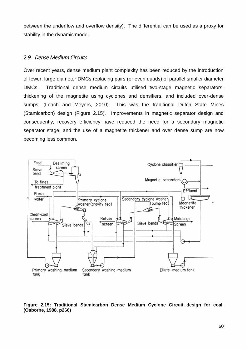
60

between the underflow and overflow density). The differential can be used as a proxy for

stability in the dynamic model.

2.9 Dense Medium Circuits

Over recent years, dense medium plant complexity has been reduced by the introduction

of fewer, large diameter DMCs replacing pairs (or even quads) of parallel smaller diameter

DMCs. Traditional dense medium circuits utilised two-stage magnetic separators,

thickening of the magnetite using cyclones and densifiers, and included over-dense

sumps. (Leach and Meyers, 2010) This was the traditional Dutch State Mines

(Stamicarbon) design (Figure 2.15). Improvements in magnetic separator design and

consequently, recovery efficiency have reduced the need for a secondary magnetic

separator stage, and the use of a magnetite thickener and over dense sump are now

becoming less common.

Figure 2.15: Traditional Stamicarbon Dense Medium Cyclone Circuit design for coal. (Osborne, 1988, p266)

61

Modern control loops are often set up as a rising density system where water addition is

made via a control valve at the exit of the correct medium sump and controlled by a

feedback loop from the nucleonic density gauge in the same line (Figure 2.16). The

advantage of this design is the fast response time for density adjustments. The

opportunity to directly add magnetite into the correct medium sump from the magnetic

separators reduces the need for an over dense sump, and hence results in a smaller plant

footprint. (Leach and Meyers, 2010)

Figure 2.16: Typical modern rising density system design for coal (Crowden, et al. 2013)

The system used at New Acland CHPP is a rising density system (Figure 2.17). No over-

dense sump or magnetite thickening circuit exists. Fresh magnetite is pumped directly into

the correct medium sump, and return magnetite, recovered from the magnetic separators,

also flows directly into the correct medium sump. Density adjustment occurs at the exit of

the correct medium sump via a clarified water control valve linked by a feedback loop to

62

the nucleonic density gauge further down the correct medium line. Coal is mixed with

correct medium at the oversize launder of the desliming screen and enters the DMC wing

tank. It is then pumped directly into the dense medium cyclone. The dilute sump takes

feed from the bleed valve on the correct medium line and also from the rinse side of the

drain and rinse screens and includes centrifuge effluent and floor sump effluent. The

dilute sump is pumped to the magnetic separator and concentrated magnetite returns

directly back to the correct medium sump.

63

Wingtank Feed

MagSep Effluent (Nonmags)

MagSep Feed

DMC_FEED

Correct Medium Bleed

DMC Reject

MagSep Concentrate

Floor Sump

Pump

Correct Medium Sump

Magnetic Separator

Product Drain & Rinse

Reject D&R

Screen

MagSep Feed Pump

DMC Wing Tank

DMC

SPLITTER

Magnetite Pit

Water Header

Coarse Feed

To Fines Circuit

Feed

Deslime Screen

Water to Deslime

DMC Floats

Fresh Magnetite

Water to Mag Pit

Water to MagSep Feed

Hose to Floor Sump

Reject

Product

Floor_Sump Water

Water to Reject D_R

Correct Medium

Drain return

Figure 2.17 The New Acland Plant 2 DMC circuit is shown pictorially below: The single stage magnetic separator is fed directly from the dilute sump and return concentrated magnetite is directly added to the correct medium sump.

64

Coal plant design is often influenced by the need to handle clays. The use of selective

thin-seam coal mining practices can alleviate some clay contamination in the feed,

however, in the case of Walloon coal measures, at New Acland and in the Clarence-

Moreton Basin coal region, it is not uncommon for the non-coal material to be layered

within the coal bands, therefore making total removal almost impossible. (Crisafulli, et al.

1985) “The major problem… is the distinct degradable shale bands interbedded within the

coal as thin litholitic markers usually no more than 150mm thick. These degradable bands

are composed mainly of montmorillonite with minor amounts of kaolinite and quartz.”

(Crisafulli, et al. 1985) Because these clay types tend to rapidly degrade upon

atmospheric exposure after mining, every effort is made to process the coal rapidly at New

Acland mine to avoid breakdown into highly dispersed binding clays. The New Acland coal

plant is designed with water introduced at the ROM to avoid stickiness in the feeder-

breaker, and no raw coal stockpiles exist.

The New Acland CHPP has two single-stage plants, the first is a Jig, DMC and spirals

circuit, and the second, known as Plant 2, is a DMC and spirals circuit. The JKMRC and

CSIRO instruments that have been set up to monitor the dense medium circuit have been

installed in Plant 2. Raw coal feed to Plant 2 is transferred by conveyor from the feeder

breaker into a secondary and tertiary sizing station at the rate of 550 tph. The coal

passing through the sizer drops directly into a sump and is pumped with water addition

(from clarified water and magnetic separator effluent) to the desliming screen. This design

is uncommon. Generally, the coal would be conveyed dry until it enters the plant directly

above the desliming screen. As sticky clays are prominent in this coal basin, handling

issues in the materials handling system can be reduced by adding water to the system at

an earlier point. Anecdotally, operators at the plant have described finding large clay balls

on the desliming screen. The 1.4mm aperture desliming screen separates the coarse coal

into the DMC circuit, and the fine coal passes to the spirals circuit. The beneficiated

coarse coal product is then dewatered via a basket centrifuge and conveyed to trucks

which transfer the coal to the rail system. Coarse rejects is combined with Plant 1 rejects

and returned to the mine via a rejects bin.

65

2.10 Circuit Instrumentation and Control

Density Control

Gaining a more comprehensive understanding about optimal operation of dense medium

cyclone circuits is critical to maximising profitability of coal mines, particularly in light of

falling coal prices. A collaborative effort between CSIRO and the JKMRC on ACARP

Project C17037 - Joint Evaluation of Monitoring Instrumentation for Dense Medium

Cyclones led to the successful commissioning of new instruments in the New Acland coal

preparation plant. These instruments comprised accelerometers, Electrical Impedance

Spectrometers (EIS) and magnetic susceptibility probes, and provide real-time, on-line

measurements. This range of data is the first of its kind to become available in the

Australian Coal Industry and has the potential to become the new benchmark for future

coal plants worldwide. The accumulation of long-range data is also an industry first and

provides the opportunity to look at coal plant dynamics over a long period of time rather

than relying only on spot-audits for verification.

The most common form of medium density measurement in modern CHPP is the

nucleonic density gauge. A significant drawback with this instrument is the presence of a

hazardous radioactive source which presents a risk to personnel. Nucleonic gauges are

generally reliable and require little maintenance (Cavanough 2008). Concern over the

risks of a radioactive hazard have prompted alternatives to the Nucleonic gauge to be

investigated. Cavanough et al. (2008) developed a medium density measurement device

that used magnetic susceptibility to determine density of the medium in the drain and rinse

screen underpans. This type of apparatus has been in place at New Acland Coal mine for

the past three years and has proven to be a very robust piece of equipment. Another

instrument installed at the site was developed by Sheridan (2011), and was capable of

measuring the density of a slurry circulating in a DMC unit at the overflow and underflow

points. This Through-Tile Density Meter instrument, measured the combined medium and

coal density in the DMC overflow with the presence of an air core. This device used the

Hall Effect, capitalising on the presence of magnetic material in the slurry.

Other non-nucleonic devices available include the differential pressure technique which

utilises a measure of differential pressure on a tester leg. (Cavanough 2008). Zhang

(2010) developed a Heavy Medium Suspension Density-Viscosity detection device which

66

essentially used differential pressure and was non-nucleonic. Firth et al, (2010) developed

Electrical Impedance Spectrometers (EIS) which provided measurements of the medium

density and composition. These instruments have been in place at New Acland in various

locations in the Dense Medium Circuit and have provided useful online data about the

circuit behaviour. In addition to the density measurement devices at New Acland, other

additional instrumentation was installed. Screen motion analysers based on

accelerometer technology were used for measuring screen health as well as mass flows

over screens, and a Cross-Correlation Flowmeter was installed in the DMC feed line from

the wing tank. (Firth 2010) By combining these instruments with the existing standard

CHPP nucleonic gauge and a SCADA control system, the information enabled more in-

depth measurement of circuit behaviour than had been previously accomplished in the

past.

There have been some drawbacks to monitoring coal dense medium circuits using existing

standard plant instrumentation. Traditionally, plants used density measurement and

controlled sump volumes and DMC pressure to obtain a satisfactory operating circuit.

Pumps were either single speed or variable speed drives, with current trends gravitating

towards variable speed drives to maintain DMC pressures. This introduced another

dynamic variable to the system. Mineral Matter (commonly referred to as Ash)

measurements were manually fed back to the control room and adjustments to density set

point on the DMC circuit were made to change the ash result. The time taken for samples

to be analysed caused a lag to occur before a plant correction was made. During the time

period that a sample was being analysed, the plant may have processed a number of

thousands of tonnes of coal. In many plants where ash was critical, sampling was

conducted on an hourly or two hourly basis, but some plants only sampled on a 12 hourly

basis. In this period, the amount of coal processed could have been as high as 10000

tonnes between ash adjustments. Some plants were less concerned with controlling ash

and were able to blend to achieve a satisfactory product, however others required the

density to be tightly controlled. Attempts to address this problem were mostly focused

around installation of on-line ash gauges, however, these have been met with limited

success in the coal industry, and in most successful cases, on-line ash gauges have been

installed in single seam operations with minimal variation. The author has not yet

encountered a coal processing plant that has been able to exclusively rely on an online

ash gauge for the purposes of plant density control.

67

Outside of the limited instrumentation provided in most plants, little is known about how a

circuit changes with variations in feed, and in particular, how the medium varies in a

dynamic sense. Recent work by Addison (2010) has enabled a better understanding.

Addison installed additional nucleonic density gauges around a circuit to monitor feed,

overflow and underflow density and to look at the relationship between measuring density

with coal present in the stream and without coal present in the stream. Typical circuits in

the USA have a draft tube arrangement where medium and coal are present where the

nucleonic gauge sits and this has been found to give different measurements when

compared to wing tank arrangements such as those present in many Australian coal

plants. With a wing tank arrangement, the medium is measured separately to the medium

and coal slurry.

Addison (2010) looked at responses to changes in plant feed, and in particular, to low

yielding versus high yielding coals at Tom’s Creek mine in Virginia, USA. Critically,

Addison identified that when high amounts of reject material were present in the coal

medium mix, the nucleonic density measurement for a coal and medium slurry was

significantly different from a nucleonic density measurement for a medium-only slurry. It

was proposed that the presence of a large amount of reject material in the medium had an

influence on the density reading as the nucleonic gauge interpreted the presence of large

amounts of high density rock as over-dense medium. Addison recommended that future

plant designs include a means of measuring the ‘true’ density of the medium without coal

present as is typically done with Wing tank design plants. Addison also recommended the

recombination of return medium streams from drain and rinse screen under-pans (product

and reject) and using this stream to analyse medium density.

The use of nucleonic gauges as in Addison’s work led him to conclude that gauges should

be installed on the medium return lines, however current installations of JKMRC and

CSIRO instruments at New Acland have advantages over nucleonic technology as they do

not require changes to head-room due to their compact nature, and they are non-

radioactive. Addison did not consider the role that non-magnetics may play in the

stabilization of the medium circuit.

Phillips (2010) performed a steady-state desktop analysis using a spreadsheet to compare

advantages and disadvantages of heavy media circuit control. He looked in particular at

bleed and sump volume fluctuations. He mentioned the importance of focusing on density

68

rather than correct medium sump level and he noted that the sump level should be allowed

to fluctuate so that density can be better controlled. Phillips looked at both a rising and

falling density systems for comparison. The rising density system is commonly in use in

modern plants as it allows faster response time to density fluctuation by means of an

automatic water valve at the inlet to the correct medium pump. This is the same system

that is in place at New Acland. Phillips profiled the effects of upsets on the dense medium

circuit, such as feed changes, adjustments of the bleed, higher water addition with the

feed, and the difference between the addition of density control water with and without the

bleed operating. He found that the operation of the bleed could assist with reducing the

requirement of density control water. His analysis of changes in feed size distribution

found that a finer feed could lead to subsequent short-term overloading of the magnetic

separator with a subsequent loss of magnetite. Phillips did mention the effect of non-

magnetics on influencing density, stating that when the plant feed is off, the rapid drop in

density could be partially attributed to a loss in non-magnetics by bleeding to the magnetic

separator. His consideration of the effect of non-magnetics however, was fleeting and was

focused on high media viscosity and poor separation, not on medium stability. His study

was essentially a steady state balance and apart from a few test conditions, it did not

examine dynamic changes with time.

Plants are typically designed with minimal capital expenditure and minimal footprint in

mind. This drives sumps to be designed for minimum volume capacity. The outcome is

that during extremes of plant operation, there is little room for error. Tight constraints on

sump capacities exacerbate the influence of volume on plant control. In the operator’s

drive to limit spillage and avoid the plant feed cutting off due to insufficient sump volume,

levels in sumps are typically maintained within a specified range. The bleed valve to the

dilute sump is often used for the purpose of adjusting correct medium sump level. By

operating the bleed valve in this manner, the volume in the sump will change, however, the

level of non-magnetics can also drop without the operator’s knowledge. There exists a

trade-off between operating for stable volume and for optimum density. The key lever in

plant performance is of course, density, and as Phillips (2010) states in his study,

positioning the bleed system manually and letting the sump level float provides a tighter

density control than if the focus were to be on controlling the bleed for sump level.

When a density change is required, volume control becomes critical. For instance, if the

density is lowered, additional water will automatically be introduced into the system,

69

thereby increasing the level in the correct medium tank. If there is insufficient room in the

correct medium sump, the operator will likely increase the bleed to reduce level. Firth et

al. (2014) explored the effects of non-magnetics levels during plant operation from start-up

conditions. When the bleed is opened, the operator is generally unaware that the open

bleed can leave insufficient non-magnetic material in the correct medium, because the

control system does not show them that the level of non-magnetics is dropping. Although

the density of the medium may respond relatively quickly, within say, ten minutes, the non-

magnetics concentration can take some time to recover. Figure 2.18 demonstrates the

time taken for a coal circuit to recover from a plant shutdown with non-magnetics levels

experimentally determined.

Figure 2.18: Comparison of % non-magnetic material in the correct medium after a plant start up over time. (Firth et al. 2014)

In this particular case, it took more than sixty minutes before the non-magnetics level

stabilised. In some cases, if the correct medium bleed to the dilute circuit is left at a high

rate, the system may not recover and non-magnetics could reach a level where the system

becomes unstable and the DMC surges.

70

2.11 Modelling and Simulation

In recent times the constant challenge to improve business profitability has driven an

increased demand for dynamic modelling expertise. The availability of online

instrumentation and connection into plant control systems have enabled more inputs to be

analysed and interpreted. Models developed in the past, while still relevant today, were

constructed with less available information and in older programming languages such as

Fortran. The process layouts of the plants studied at that time were also somewhat

different from the more modern designs. The improved capability of current modelling

software has broadened the potential for more in-depth analysis in dynamic computer

models. Plant designers have historically used steady state modelling for design and

construction purposes, however insights from online instrumentation could be extremely

valuable, particularly in terms of designing for changing circumstances in a coal plant such

as a seam change. While steady state models assume many constants, in practice, many

of these parameters shift in real time. The ability to see the magnitudes of the shifts and

the downstream effects can be better observed using dynamic modelling. The following

section will review existing models and modelling methods in common use and review the

reasons why a dynamic model is required in this project.

In 1982, Lyman et al. developed a dynamic model of a DMC circuit at Westcliff Collieries.

The research included interfacing of plant control system instruments with a computer to

log plant data. The model divided the dense medium circuit into individual units of

operation and performed calculations around each unit. A number of important

assumptions were made in this model. It was found by experiment that sumps behaved as

variable volume plug flow devices. The DMC was found to have virtually no residence

time and was therefore modelled as a pipe. The drain and rinse screens were assumed to

have perfect recovery of magnetite on the rinse section with a second assumption that the

coarse screened material moisture content at the desliming screen was the same as the

moisture content at the drain and rinse screens. The volume of medium carried on the

coal from draining to rinsing was calculated as a function of coal surface area and rinse

water rates were held constant. The magnetic separator model used was determined

based on earlier work by Davis (1981). His model used an experimentally determined

percentage recovery based on the mass flow to the magnetic separator. Stream splitters

71

were assumed to have no delay and were designed as a pre-determined proportional split

of the incoming stream.

This early work was critical to control system design, particularly with respect to modelling

locations for water addition points into the correct medium for improved density control.

The research of Lyman et al (1982) was further developed to form part of Askew’s (1983)

Fortran model. While Askew was also involved in Lyman et al.’s earlier work, he modelled

an additional site, Buchanan Borehole Colliery in his later research. These circuits were

not identical to the New Acland design, and in some cases were two-stage operations with

a primary and secondary product. Askew’s research into water locations for density

control led to the simulated change to the design of water addition to the dense medium

circuit at Buchanan Borehole Colliery being successfully implemented in the plant, with

resulting improvements in density response time.

Both of the dynamic models used by Lyman et al. and Askew were structured using

discrete volume elements of data expressed in an array format, with each volume parcel

containing specific properties. At each time step, a volume parcel was moved into the pipe

or unit of operation, and another parcel of equal volume removed. Multiple components in

each stream were dealt with by creating dummy pipes in parallel. Throughout the time

steps, each volume parcel retained its properties and the time taken for the parcel to reach

the exit of that particular unit of operation was determined based on the variation in

flowrate into the unit. All elements were considered to be full with the exception of the first

and last elements (inlet and outlet) which had a combined volume equal to one full

element. The properties in each volume exiting the unit were calculated from previous

volume parcels. This volume parcel concept has been adopted for the development of the

new dynamic model.

The key deficiency in Askew and Lyman’s research was that the modelling of components

did not consider the behaviour of non-magnetic components in the medium, but rather,

simply modelled magnetite and water. The unit operations modelled used simplified

models that required tuning to plant data, and it was acknowledged that further

improvements could be made to the unit operation models in future research. Since this

research was completed in the 1980’s, considerable advances in empirical models have

occurred, leading to better prediction of plant behaviour and new opportunities for dynamic

modelling.

72

Following on from Askew’s work, Wiseman et al. (1987) developed, and tested a dynamic

model of a coal preparation plant and verified the data using plant audits and an on-line

ash gauge. The model comprised menu driven operation to select unit operation models

from a library. In addition to DMCs, other types of coarse coal processing equipment were

also modelled. The dynamic model also extended beyond the coarse coal circuit to include

other aspects of CHPP operation such as size classification, fine coal and feed

washability. It was noted that computer memory was a limitation of the research, and this

drove innovative solutions to handling of washability data for streams using arrays and

mathematical models. Unit operation empirical models available for this research were still

limited and have been considerably improved since this time.

The body of research by Wiseman et al. (1987) is still useful as a general model and

formed the basis for JKSimMet and JKSimCoal steady state models. The work of

Wiseman also led to the development of LIMN steady state software. It is now very

common for CHPP designers and coal producers to use LIMN as their standard software

package. The advantage of LIMN for coal use is its user-friendly structure in a familiar

Microsoft Excel software program. More simulation software such as JKSimMet and

JKSimFloat exist for metalliferous applications, but the need for this level of complexity in

coal has not yet been identified. Many other steady-state modelling software options exist

and are applicable to the coal industry. The use of LIMN has prevailed over the past

twenty years due to its ease of use and coal-specific design. LIMN however, does not

have a dynamic modelling component. Dynamic models of coal plants have been fewer in

number, and their use has been relatively limited. There is, a general growing interest in

dynamic modelling in the coal industry at the moment. Its potential to model from mine to

port with multiple complex variants allows great flexibility and insight into a coal operation.

The interest in dynamic modelling has led to further research by Meyer (2010). Meyer

dynamically modelled and verified a coal preparation plant at Leeuwpan Colliery in South

Africa using Matlab Simulink. His approach was from a process control perspective and he

did not appear to have the benefit of a coal preparation background, and therefore was

reliant on the plant metallurgist for practical input. Meyer and Craig (2011) then developed

a steady state partition curve from the dynamic model. The use of a dynamic model to

create a steady state model also seemed somewhat superfluous from a coal processing

73

viewpoint given that many steady state models already existed and provided good

predictions.

Meyer derived equations for the dynamic model from first principles and used verification

from spot audits, however, it is surprising that Meyer did not fully utilise historical empirical

models such as (Wood et al, 1989 and Wood, 1990) that were experimentally determined

for relatively small DMCs based on significantly more coal data than that used by Meyer

(2010). The fine coal DMC circuit studied at Leeuwpan had significant complexity, and

some areas of the model were simplified. For instance, in Meyer (2010) the medium

components were not considered in the model, and the dynamic model simulated

underflow and overflow densities based on the work of He and Laskowski (1993) rather

than measuring actual values in the Leeuwpan Colliery. The work of He and Laskowski

was conducted in a laboratory environment and therefore may not have provided a close

fit to data from the South African coal wash plant itself.

Meyer and Craig (2014) then extended the model to encompass the coarse coal DMC

circuit and to create a steady state model. The testwork completed for the coarse coal

circuit simulation looked at only two plant validation cases; one where the plant feed was

varied but the medium density was held constant, and the other where the medium density

was varied and the tonnage held constant. Meyer noted that the degree of influence from

the two verification audits was far greater for the medium density variation than from the

tonnage variation. It has however been widely acknowledged in the coal industry for some

time that a medium-based model (Wood et al. 1989) is appropriate for a dense medium

cyclone circuit as the medium has a strong influence on DMC behaviour. This has been

further supported by more recent work by Firth et al. (2014).

A number of factors were assumed by Meyer to be constant due to lack of information, for

example, the coarse material feed rate to a module was calculated as the difference

between the primary screen feed and the oversize feed, feed rates to the circuit were

weighted based on weightometer readings from the total plant feed which incorporated

significant noise. Meyer also assumed that the volumetric flowrates of the feed, between

underflow and overflow were constant before and after a step was introduced to the

medium density or feed rate. He used product yield and product quality data from the

Leeuwpan Coal plant to determine whether or not there was an opportunity to improve or

optimize the process control system. Product yield data however, was hampered by

http://et.al/

http://et.al/

74

weightometer inaccuracy and the lack of measurement points within the actual DMC

circuit. The feed rate of coal to the DMC mixing box was not measured and therefore

estimations had to be made based on screen splits using expected particle size

distribution rather than from in-plant sampling. Similarly, the density of the mix was not

measured and DMC inlet pressure was used for indication, however other factors such as

sump level changes, surges or uneven feed of coal from de-sliming screens and pump

cavitation could have influenced the values. Medium density was measured but medium

behaviour was not modelled.

A simulated output of overflow and underflow densities was modelled, but Meyer (2010)

proposed that the increase in differential was due to the feed being reduced, ie. a change

in medium to coal ratio. Meyer did not delve further into this and quite likely would not

have realised that the increase in differential could have been related to the loss of non-

magnetics from the system via the bleed line if tonnage dropped but bleed levels remained

constant. The change in differential also seemed to track the water and magnetite model

where the water valve closed while density was increased which logically would have

resulted in a gradual increase in magnetite concentrate returning from the magnetic

separator into the correct medium without a corresponding increase in non-magnetics as

plant feed rate dropped. Meyer’s work from 2010 was verified with only one audit, and the

latter work in 2014 with an additional two audits, only one of which used a change in

medium density. This verification may therefore not hold across all plant situations.

While components of the feed were considered by Meyer according to the principle of

conservation of mass, these were limited to ash, sulphur, moisture, medium and fixed

carbon components without detailing medium constituents such as non-magnetics. It was

found that the model did closely approximate the results found in the spot verification

audits, most data points of which were taken from the control system. Meyer's recent work

highlights the lack of adequate information and measurement systems available in dense

medium circuits and in coal preparation plants in general. He recommended further work

on a longer-term basis to do additional verification of his model.

In the above research efforts, a lack of adequate online information hampered research

efforts. Verification was by snapshot audits due to a lack of long range data. The models

did not attempt to model non-magnetic components in the medium. Accurate

measurement of changes to the dense medium proved difficult due to the absence of

75

sufficient instrumentation. By comparison, the New Acland instruments adopted for this

project allowed the modelling work to be advanced as the in-stream monitoring of drain

and rinse screen underflows, the correct medium, screen mass flow rates and DMC feed

flow rates could be incorporated with traditional plant instrumentation to obtain a far more

comprehensive understanding of what happens over time. Previous modelling efforts also

focused on smaller diameter DMCs whereas the New Acland DMCs, being a larger

1300mm diameter, yielded considerably more large DMC data for modelling.

The use of a dynamic model for coal preparation has not become commonplace, largely

due to the high level of complexity and cost required to set up the models. For

engineering design purposes, steady state modelling has provided sufficient

approximations to achieve a satisfactory design. The advantage of dynamic simulation

however, is the ability to achieve optimisation of control circuits and to make incremental

adjustments for the plant to perform at optimum levels for a higher proportion of the time.

The incremental losses from poor instantaneous performance can compound into

significant yield losses over time. Capturing these incremental gains can greatly enhance

profitability.

Non-coal examples of dynamic modelling include alumina and petrochemicals. SysCAD

was used at the Yarwun Alumina Refinery in Gladstone for both plant design and

operations, the latter use including the training of control room operators on a simulator.

This has proven to be a very useful mimic of the real plant operation. Pilot tests can be

run using dynamic models without the high cost of plant trials or without potentially

dangerous consequences of a plant incident occurring. The Yarwun example has given

the author confidence that the dynamic model’s potential as a training tool and for testing

control system changes will be extremely valuable. Similar examples exist in

petrochemicals for operator training systems and dynamic models for advanced process

control.

76

2.12 Literature Review Findings

Although dynamic models have been built in the past for Coal Handling and Preparation

Plants, most notably Lyman et al. (1982), Askew (1983), Wiseman et al. (1987) and Meyer

(2010), modelling of changes in the coal medium and non-magnetics have not been

sufficiently studied. Development of dynamic models has been limited in the past by a

lack of available plant data, computer memory and processing capability. Currently

available technology allows far greater processing power and software capability. Novel

instruments installed at the New Acland CHPP allow information to be collected that was

previously unavailable. New experimental procedures using RFID density tracer

technology provide additional plant data such as residence times for individual particles.

Empirical models for DMC circuits such as those detailed in Crowden et al. (2013) have

been significantly improved since early modelling work was done and a wider range of

plant information is now able to be collected. Recent studies of changes in DMC medium

composition within and between plants (O’Brien, et al. 2013) have shown that the level of

non-magnetics influences medium stability when targeting a low density cut-point and

therefore has an influence on plant behaviour. This new knowledge of non-magnetics will

also be integrated into a dynamic model.

The outcome of this research will be a dynamic model of the New Acland dense medium

circuit which, supported through experimental results and existing empirical models, better

explains the behaviour of a dense medium circuit. The model will utilise existing empirical

relationships that are accepted by industry as providing reasonable predictions of plant

behaviour. Non-magnetics concentration in the medium will be predicted using a

breakage model and results will then be verified against past plant event data collected

during the experimental work stage.

This research differs from past research efforts in that novel instrumentation and

techniques have been used to collect experimental data, and the inclusion of medium

components to predict the proportion of non-magnetics in the medium has not previously

been attempted. Changes that result from fluctuations in magnetite additions, density

adjustments and the bleed valve which diverts non-magnetics to the magnetic separators

77

can also be incorporated into the dynamic model. The dynamic model can then be used to

guide operators to better understand DMC circuit behaviour.

A dynamic model will provide coal producers with critical drivers for optimal dynamic DMC

circuit performance and operator training. Plant observations and physical measurements

will be used alongside on-line data to verify the model. Samples of the medium, analysed

for %non-magnetics will be incorporated into the dynamic model. Benefits derived from

this project include potential improvement of plant profitability through better utilisation and

optimal operation of dense medium circuits and improved understanding of dense medium

circuit fluctuations.

78

Experimental Work

3.1 Process Description

Numerous site visits to the New Acland coal handling and preparation plant (CHPP) were

conducted over the course of the research. Some visits were for the purpose of plant

observation and discussion with plant personnel. This provided valuable insight into the

circuit operation and limitations. Other visits were on designated test dates with sampling

and subsequent analysis. The author would like to acknowledge the work of the control

room operators who obligingly operated the plant to test the various case conditions. The

New Acland plant consisted of two separate modules. The focus of the PhD was on Plant

2 dense medium circuit. A schematic of the plant 2 dense medium circuit is shown in

Figure 3.1.

Concentrate

Correct Medium

Wing Tank

Dilute

Desliming

Reject Product Product

Water

Bleed

To Magnetic Separator

Effluent

DMC

To Desliming Water sump

Gauge

Raw coal Feed

Figure 3.1 The New Acland Dense Medium Circuit plant 2.

79

Plant 2, which processes approximately 550 tph of raw coal, is comprised of a single-stage

DMC circuit treating the deslimed coarse material which is minus 50mm by 1.4mm w/w

(wedge wire) material. The minus 1.4mm w/w material reports to the spirals circuit. The

plant does not have a flotation circuit and thus, the minus 150 micron material reports

directly to the thickener. The deslimed coarse raw coal is mixed with medium after the

desliming screen and enters the coal side of the wing tank. The wing tank is split into two

parts, the coal side which pumps to the DMC, and the seal leg side which overflows back

to the correct medium sump. The two sides of the tank are separated by an orifice plate

and normal operation is for medium to flow downwards through the orifice plate from the

seal side into the coal side. The drained medium returns to the wing tank via the seal side,

and a portion of this overflows into the correct medium sump. The wing tank coal side

pumps to the DMC and the overflow reports to the product drain and rinse screen. The

underflow of the DMC reports to the reject drain and rinse screen.

The coarse coal product is then centrifuged and sent to the stockpile. The coarse rejects

are transported to the rejects bin and are then transferred back to the mining pit waste

area. The underflow from the drain and rinse screens is split with the drain sides

combining and returning to the seal leg of the wing tank, while the rinse underpans are

combined and sent to the dilute sump which then pumps to the magnetic separator. The

effluent of the magnetic separator returns to the desliming water sump at the start of the

process. The concentrated magnetite from the magnetic separator is returned to the

correct medium sump. Within the dense medium circuit, a rising density system exists.

The outlet of the correct medium sump has a water addition valve which is controlled in a

feedback loop to the nucleonic gauge which is situated further down the correct medium

line. When the medium density is too high, the water addition valve opens to dilute the

medium density. When density is too low, the water addition valve shuts.

A bleed line exists in the correct medium line between the automatic water addition valve

and the nucleonic gauge (Figure 3.2). The butterfly valve on the bleed is controlled

manually by the control room operator. The bleed line runs directly to the dilute sump.

Controlling the bleed valve enables the operator to control volume in the correct medium

sump, but also enables non-magnetic material to be removed from the medium in the

magnetic separator, thereby concentrating the medium density. The bleed line is a

nominal 100mm diameter pipe which rises approximately 500mm directly above the

80

correct medium pipe which is 330mm diameter and oriented in a horizontal plane. There

are three elbows in the line from the pump to the bleed take-off therefore segregation due

to bends is possible. As the bleed take off is on the top of the correct medium pipe

approximately 1500mm from the preceding elbow, particles could also segregate in the

horizontal pipe allowing lighter density floating particles to flow up into the bleed line. The

installation of the nucleonic gauge on a horizontal plane is also not ideal.

100mm

diameter

0.3m

1.5m

3.6m

elevation

from

pump

outlet

on

ground

floor

Three elbows between

pump and bleed line

Butterfly Bleed Valve

Correct Medium Line

330mm diameter

Nucleonic Gauge

Figure 3.2: An elevation view of the piping layout for the bleed split to the dilute sump in the correct medium line.

Prior research by O’Brien et.al. (2013) has demonstrated that the level of non-magnetics in

the medium is important and therefore, the function of the bleed valve is integral to

successful DMC circuit operation. The program of experimental work outlined below has

incorporated monitoring of the bleed valve in order to assist with developing a dynamic

plant simulator.

81

3.2 Outline of Experimental Research

The literature review has identified a number of areas in which further research is

warranted. It was established that there is a need to better understand the behaviour of

non-magnetics during various plant events. Depending on seam variation and mining

method, the plant feed can vary widely, triggering a wide range of plant operating set

points. For instance, a plant feed change could lead to a change in density target from

1.30RD to 1.60RD, or a step down by a similar amount. This plant feed variation, coupled

with technical marketing product ash requirements, can necessitate multiple density set

point changes per day. The broad range of plant feeds at New Acland mine means that

changing the density set point is a regular occurrence. The corresponding plant

responses to large and small changes, as well as incremental changes, has not been

widely documented. Quantifying the cumulative yield impacts of density changes is

expected to lead to generation of ideas for better circuit control and management and a

consequential reduction in yield losses. In terms of non-magnetics, it is only through the

collaborative work with CSIRO that plant responses are now being measured.

Measurement of the changes in non-magnetics aligned with plant events will also assist in

better plant control, and will provide vital data for the dynamic model.

A number of tests were devised to assess plant behaviour under changing plant

conditions. The difference between a single step change and an incremental change in

density, and the difference between an increase and a decrease in density need to be

assessed based on the plant response. Similarly, the effect of an unstable environment,

with overflowing sumps, and the plant operating at its density extremes would yield useful

information about how the plant copes and how long it takes to return to stable operation.

Finally, the observations made of the New Acland plant during the course of this research

and the related body of collaborative work has suggested that the operation of the bleed is

often done for volume control, not for metallurgical control and that the effect of the bleed

operation on non-magnetics concentration in the medium needs to be further quantified.

Reviews of prior research did not reveal the time taken for coal particles to travel through

the coal washery, nor how long some particles may linger in the dense medium circuit. A

82

test therefore needed to be devised to determine residence time for the model. Using

recently developed technology radio frequency identification (RFID) density tracer

technology, a new application was found. If the RFID density tracers, each with individual

identifier tags, were timed as they travelled through the circuit, it would be possible to

achieve residence times for each individual particle. This information could then feed into

the dynamic model as a delay or time-lag measurement. The presence of two different

sized tracer particles, 13mm RFID tracers and 32mm standard tracers also offered an

opportunity to investigate the relative differences between particle size, cut-point and

efficiency by developing partition curves.

A number of test cases were established for data collection at New Acland site. These

cases were determined from specific events observed in previous instrument data

collection. A summary of the test cases is given below:

Case A: Good density change.

This test intended to ascertain how the plant would respond in a stable situation where a

controlled density change occurred with minimal instability. This test also considered a

controlled bleed volume to ensure that the non-magnetics remained relatively constant. A

plant with well controlled levels in sumps and no feed interruptions was also required for

this test. The test then aimed to follow what happened to the density and the

concentration of non-magnetics when plant was initially in a stable condition and a

controlled change occurred.

Test: Following a stable transition of density in the dense medium circuit, collect correct

medium samples at 10 min intervals for an hour and then for 20min intervals for 2 hrs

thereafter. Analyse for the proportion (dry weight %) non-magnetics, density, and particle

size.

Case B: Unstable Volume.

When plants are operating at a low density set point, a situation can arise where volumes

are unstable. The amount of water in the system is too high and the sumps overflow. The

cause of this, is the inability of the circuit to rid itself of excessive magnetite in the system.

83

If there is a high level in the correct medium sump due to a change from high density to

low density, the water valve on the correct medium sump compensates for the

concentrated magnetite being added back into the correct sump from the dilute circuit.

This can lead to an overflow situation, however the overflows return magnetite to the dilute

which recycles back into the correct sump via the magnetic separator, thereby leading to

further water addition. It can take some time for the plant to regain stable sump levels

after this type of density change, particularly if the previous density set point was high.

This test aimed to look at the plant response to such a change in terms of the level of non-

magnetics and the time for the density to reach set point. The test also looked at the effect

of changing bleed levels during this type of situation.

Test: High level in the correct medium sump and a high level in the dilute sump before

density drop. Open Bleed to 100%. Collect correct medium samples at 10 min intervals

for an hour and then for 20min intervals for 2 hrs thereafter. Analyse for the proportion

(dry weight %) non-magnetics, density, and particle size.

Case C: Stepwise density change:

While normally a density change would be done in one single step, eg. 1.3 to 1.4, or from

1.4 to 1.6, it was noticed that some operators prefer to step the density up in increments.

The effect of stepping up in increments compared with a standard single step was tested

using this case.

Test: Measure the time for the circuit to recover from a density change (Rise / Fall) after a

large step change in density. Do the same for a change in small increments. Collect

correct medium samples at 10 min intervals for an hour and then for 20min intervals for 2

hrs thereafter. Analyse for the proportion (dry weight %) non-magnetics, density, and

particle size.

Case D: The low density stability test:

The intention of this test was to investigate the behaviour of the circuit in a low density

situation where there was an unstable level of non-magnetics in the medium. Testing of

the case required certain conditions to be present in the plant. The plant would need to be

operating below a density of 1.40RD, and there needed to be a relatively low level of non-

84

magnetics in the system. In essence, a high differential, and potential surging situation.

The test was then intended to add back non-magnetics into the system and measure the

effect.

Test: Running on a low density set point, open bleed fully. Collect correct medium

samples at 10 min intervals for an hour and then add non-magnetics to the system by

adding thickener underflow. Measure Collect correct medium samples at 10 min intervals

for an hour and then for 20 minute intervals for approximately 2 hours thereafter. Analyse

for the proportion (dry weight %) non-magnetics, density, and particle size.

In practice, the aims of this particular test were only partially achieved due to plant

conditions not being ideal at the time. While a low density target was achieved, the plant

had significant quantities of non-magnetics present in the medium and was therefore not

running at a high differential at the time.

Case E: Desliming sprays response test:

The intended aim of this case was to assess the plant response when an increased

amount of clay slimes entered the dense medium circuit due to reducing the spray water

on the desliming screen. Reducing sprays on the desliming screen had the effect of

diverting some slimes adhering to the coarse coal over into the dense medium circuit. The

effect of the change on the proportion of non-magnetics in the medium was then

monitored.

Test: Running on a low density set point, open bleed fully, hose in magnetite, Collect

correct medium samples at 10 min intervals for an hour and then add non-magnetics to the

system by turning off desliming sprays. Collect correct medium samples at 10 min

intervals for an hour and then for 20min intervals for 2 hours thereafter. Analyse for the

proportion (dry weight %) non-magnetics, density, and particle size.

Case F: Tracer testing and determination of residence times in the DMC circuit

Partitioning Test: Insert a range of densities of 13mm and 32mm tracer sizes into the DMC

circuit and compare partition performance.

This case was intended to measure both partitioning performance and the time taken for

coarse coal particles to travel through the dense medium circuit. The full range of standard

85

tracer densities were inserted concurrently with the RFID tracers at the desliming screen.

These were collected at the drain and rinse screens either via the antenna detection or by

manual collection in the case of the standard tracers.

Residence Time Test: Insert a selection of 13mm RFID tracers at various densities into the

dense medium circuit to analyse times for coarse particles to travel through the various

sections of the DMC and dilute circuits.

As the RFID tracers contained a variety of densities, it was possible to measure the effect

of density on residence time, both in the coal and medium circuits. Tracers of three

different densities; one high, one low, and one density close to the medium density were

inserted. The RFID tracers were inserted in a number of locations throughout the dilute

and correct medium circuits and were detected using the antennas on the drain and rinse

screens. This gave information about the relative times taken for particles to travel

through the different routes in the DMC and dilute circuits.

86

3.3 Experimental Results

The outcomes of the various cases studied are detailed below:

Case A: Good density change.

Test: A stable transition of density in the dense medium circuit

On 14th June 2013 and 24th October 2013, correct medium density was monitored. The

24th October 2013 also coincided with a tracer test run. On the 14th June event, the level

of non-magnetics was monitored and the figure 3.3 below demonstrates the results.

Figure 3.3: %Non-Magnetics measured on the day of the good density change trial

The following dot-points give a chronology of events:

At t=0mins, which was 10 mins prior to the density change, a sample was taken of

the medium

At t=6 mins, the density was raised from 1.367 to 1.410 on the control panel

At t=14 mins, The bleed valve which bleeds correct medium to the dilute was fully

opened for one minute and then closed at 40% (previously it was 30%)

At t=31 mins density was decreased from 1.410 to 1.398

Between 40mins and 42mins the plant feed dropped off and then recovered

87

In Figure 3.3, the level of non-magnetics decreased as the bleed level was increased. The

increase in density target would have also required additional magnetite which would have

had low levels of non-magnetics associated in the fresh magnetite feed. This suggests

that the choice of 40% open was too high and led to a loss of non-magnetics over time.

The loss of non-magnetics was then exacerbated by the feed off event at the 40 minute

mark. The differential of the cyclone remained steady however, and was well within the

normal operating range (approximately 0.2). Despite the plant operation of the density

change being done carefully, the reduction in non-magnetics was still quite pronounced

with an increase in bleed valve opening. This indicated that the magnetic separators have

the ability to rapidly change the amount of non-magnetics present in the medium, and also

that feed off events can be severely detrimental to % non-magnetics. While this is a stable

operation case, if the density target had been around 1.3, then the system potentially could

have had a wider differential. This case also highlights that it can take a considerable

period of time for non-magnetics to build up again in the system. In this particular case,

the non-magnetics had still not reached its original level after sixty minutes.

88

Case B: Unstable Volume.

Test: A high level in the correct medium sump and a high level in the dilute sump before a

density drop. Open the bleed valve to 100%.

On the 26th March 2014 the plant was found to be operating at 1.35 density and the

density set point was lowered to 1.30 at 87 minutes. A chronology of events is given in

Table 3.1. The plant had run on the previous day and night on a density set point of 1.6,

so considerable amounts of magnetite and non-magnetics were thought to still be in the

system at the time of sampling. The level of non-magnetics in the medium at the start of

the trial was found to be 14.7%. During the trial period, DMC feed pressure remained

relatively steady apart from a slight adjustment following the density change. (Figure 3.4)

Plant feed rate was variable due to normal weightometer variability, however the average

feed rate remained the same until approximately 200 minutes after which it increased by

about twenty tonnes per hour. This was a considerable length of time after the density

change occurred.

Figure 3.4: 26th March 2014 Plant conditions

Plant feed tonnage was relatively continuous during the trial at 500tph and increased by approximately 20tph from approximately 200 minutes. A density change downwards was observed at 96 minutes from 1.35 to 1.30. The correct medium sump was at maximum level.

89

Samples were taken of the correct medium from 10:30am in intervals of ten to twenty

minutes. During this time, the bleed was opened to 100% on two occasions, one at each

density set point. In both cases, the level in the correct medium sump dropped

corresponding to the opening of the bleed. The level in the correct medium sump

gradually recovered to 100% full at which point the dilute sump also returned to an

overflowing state. In the time that the bleed was fully open, the level of non-magnetics

dropped from 14.7% to 11.8% when operating on a density of 1.35, and in the second

case at a density of 1.30, the level of non-magnetics dropped from 12.1% to 11.4%. It is

thought that this second drop was less in magnitude because the system had not had

sufficient time to recover from the previous density change and from the earlier opening of

the bleed prior to the density change. This confirms expectations that the fully open bleed

would be expected to remove non-magnetics from the correct medium under normal

operation.

When the density was lowered to 1.30, (Figure 3.5) it was clear that the plant had difficulty

maintaining control at such a low density. This was partly due to the fact that the night

before, the plant had built up excess magnetite in the sumps from operating at a density of

1.6. Excess magnetite was visible in the floor sump area and suggested that the system

could not effectively rid itself of the excess magnetite while the sumps continued to

overflow. This was because the correct medium sump overflowed to the floor sump, the

floor sump pumped back into the dilute sump which then overflowed back to the floor

sump. In addition, the concentrated magnetite continued to return to the correct medium

sump via the magnetic separators which were fed from the dilute sump pump. As the

system was already struggling to achieve a sufficiently low density, the continual flow of

concentrated magnetite meant that more water was continually being added to the system

to compensate for the increasing density. This further exacerbated the existing water

balance problem. In this particular low density case, the sump control issues suggested

that it would have been useful to have a splitter box so that excess concentrated magnetite

could be returned back to the magnetite pit or to an over-dense system rather than into the

correct medium sump which generated more water addition to sumps that were already full

in order to control the density.

The non-magnetics was also somewhat unstable. Although there was a noticeable drop in

non-magnetics once the bleed was fully opened at 138 minutes, this drop in non-

90

magnetics did not sustain once the correct sump and dilute sumps began to both overflow.

The level of non-magnetics then began to once again gradually build up in the system. A

visual observation during sampling indicated that the medium did not rapidly settle out of

solution when placed in a clear measuring cylinder suggesting that the medium was still

quite stable despite the low density set point.

The results of this test case were analysed and it was found that the level of non-

magnetics dropped for both density set points when the bleed fully opened but once the

dilute and correct sumps began overflowing at the lower density, the level of non-

magnetics began to recover slightly. Once the bleed valve was returned to the normal

operating level of 20%, non-magnetics increased in the system by almost 2% to a level of

just under 13.7% (Figure 3.5). This was some time after the density change had occurred

and it is possible that the plant was beginning to return to a steady state. No surging of

the DMC was noticeable at any time during the plant trial. The overflowing nature of the

sumps during the trial at low density meant that the magnetite in the floor sump was

continually recycling back through the system, leading to difficulties achieving density and

volume control in the plant.

Table 3.1: Chronology for 26th March 2013

Relative

time Timeline for 26/03/2014

0 mins Plant operating at a density of 1.35. Bleed at normal level of 30% open. Non-magnetics was

14.71% before any changes were made.

5 mins Bleed was opened to 100% on request (not normal operating procedure)

10 mins Correct medium sump ceased overflowing to the floor sump (flows to dilute)

20 mins Bleed was closed fully (note butterfly valve still leaks when fully closed). Dilute sump was

overflowed briefly (<5mins). Correct medium sump level dropped to 90%

25 mins Correct medium sump resumed overflowing to floor sump (flows to dilute)

37 mins Density set point dropped to 1.30, bleed remained closed.

79 mins Bleed opened to 100% on request (not normal operating procedure)

81 mins Correct medium sump ceased overflowing until 12:56pm when it again overflowed.

102 mins

Bleed valve was cycled by operator. Correct medium sump continued to overflow despite bleed

valve being fully open. Valve was checked for blockage but no complete blockage was found.

Partial blockage suspected.

131 mins Bleed valve returned to 20% open by operator. (normal operation)

140 mins Plant tonnage increased slightly by approximately 10 tonnes per hour.

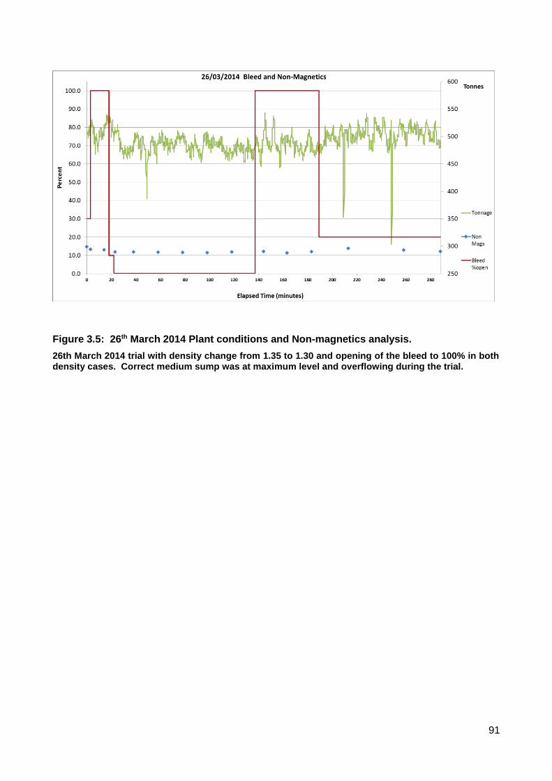
91

Figure 3.5: 26th March 2014 Plant conditions and Non-magnetics analysis.

26th March 2014 trial with density change from 1.35 to 1.30 and opening of the bleed to 100% in both density cases. Correct medium sump was at maximum level and overflowing during the trial.

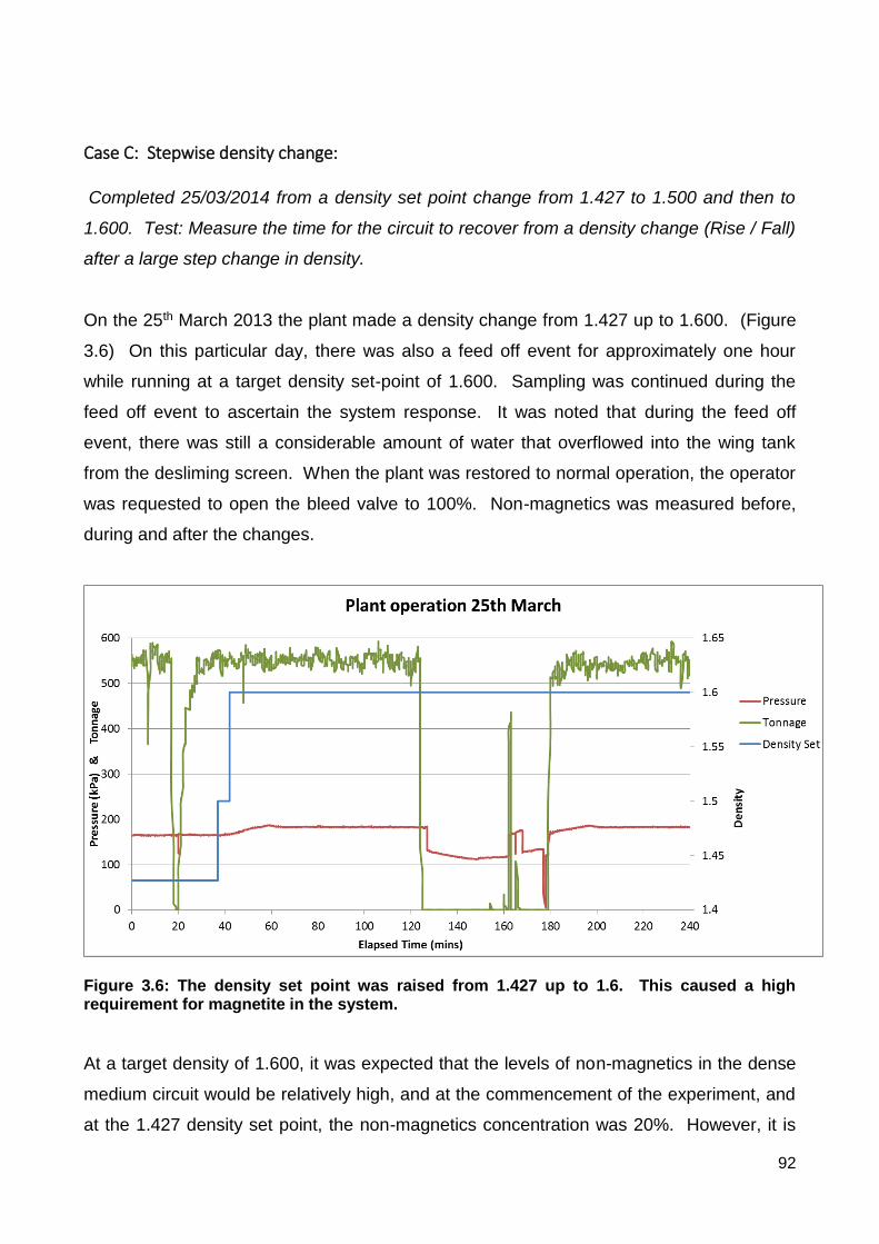
92

Case C: Stepwise density change:

Completed 25/03/2014 from a density set point change from 1.427 to 1.500 and then to

1.600. Test: Measure the time for the circuit to recover from a density change (Rise / Fall)

after a large step change in density.

On the 25th March 2013 the plant made a density change from 1.427 up to 1.600. (Figure

3.6) On this particular day, there was also a feed off event for approximately one hour

while running at a target density set-point of 1.600. Sampling was continued during the

feed off event to ascertain the system response. It was noted that during the feed off

event, there was still a considerable amount of water that overflowed into the wing tank

from the desliming screen. When the plant was restored to normal operation, the operator

was requested to open the bleed valve to 100%. Non-magnetics was measured before,

during and after the changes.

Figure 3.6: The density set point was raised from 1.427 up to 1.6. This caused a high requirement for magnetite in the system.

At a target density of 1.600, it was expected that the levels of non-magnetics in the dense

medium circuit would be relatively high, and at the commencement of the experiment, and

at the 1.427 density set point, the non-magnetics concentration was 20%. However, it is

93

known from past experiments that non-magnetics can be depleted when a feed off event

occurs, particularly if the dilute circuit continues to remove non-magnetics from the system

while no fresh coal feed is entering the circuit. A chronology of events is given in Table

3.2. In figure 3.7 the drop in non-magnetics concentration can clearly be seen to

correspond with the two feed off events observed.

Figure 3.7: 25th March 2014. Plant feed tonnage and non-magnetics.

Density change and a feed off (coal off) event occurred. The density change from 1.427 to 1.600 occurs at 37 mins. Feed off events are clearly visible when the blue line dropped to zero.

Some indications of volumetric flows were also gained on this day because the desliming

screen sprays were closed for two minutes and then reopened with a resulting change in

flowrates to the dilute circuit. The level of the dilute sump clearly changed rapidly during

this period. Within two minutes, the dilute sump volume filled from 40% to 100%. The

reason for the fast filling of the dilute sump related to the clarified water line design. The

water to the desliming screen branched off the same clarified water main as the rinse

water to the drain and rinse screens. As the valve to the desliming screen was closed,

water normally intended for the desliming screen instead diverted to the rinse screens

which drain directly to the dilute sump. This result indicated that the water balance is

extremely sensitive in this plant design. The desliming system response experiment is

discussed later in Case E.

94

Table 3.2: Chronology for 25th March 2014

Elapsed Time

Event

0 mins Pre density change. Correct medium sump (CMS) at 96%, Density at 1.427, Plant feed rate 560tph, pressure 164kPa, bleed 30% open, non-magnetics 20.1%, actual density was 1.427.

15 mins New coal type in ROM. approx. 15 mins till change filters through. Actual density was 1.431

17 mins Feed off. CMS dropped from 96% to 82% during feed off event. Bleed remained at 30% open. Actual density was 1.428

25 mins Feed on again. Bleed closed, CMS 82%, non-magnetics 15.5%, actual density was 1.435

37 mins Density changed up to 1.500 from 1.427, Bleed opened 100%, CMS at 94%, non-magnetics16.2%, actual density was 1.425

42 mins Density changed up from 1.500 to 1.600 actual density was 1.4701. Bleed 100% open, CMS 77%, Dilute overflowing by 10:39am.

47 mins Bleed changed to 20%, Density set point 1.600, CMS 55%, Pressure 172kPa, non-magnetics was 14.3%, actual density was 1.536

58 mins Bleed changed to 10%, CMS 42%, Pressure 185 kPa, Actual density was 1.633, non-magnetics was 9.6%

67 mins Bleed changed to 15% open, CMS 46%, tonnage approx. 550tph, DMC pressure 182kPa, actual density was 1.596, non-magnetics was 10.39%

77-79 mins Desliming sprays manually turned off for 2 mins then turned on again. Dilute sump rose from 40% to 100%(overflowing) during this 2 minute period. Non-magnetics was 10.7% before the change and 12.9% after the change, Actual density was 1.602

124 mins Feed off due to conveyor tracking problem. CMS 43%, DMC pressure was 184kPa, non-magnetics was 12.1% just prior to the plant feed going off. Actual density was 1.599

127 mins Bleed fully closed. Pressure dropped to 131 kPa, CMS at 34%, feed still off, Actual density was 1.600

132 mins Bleed opened to 50% to control volume, CMS at 100% overflowing, feed still off, non-magnetics at 12:10pm was 9.52%, actual density was 1.407

137 mins Bleed changed to 10% open, CM sump stopped overflowing, Operator also backed off desliming spray volumes to reduce overflow of water into the coarse launder feeding the wing tank. Feed still off, actual density was 1.386

144 mins Bleed changed to 50% open. Feed still off, actual density was 1.407

151 mins Bleed dropped to 10%, CMS at 58%. Feed still off.

153 mins Bleed opened to 50%, CMS at 48%, actual density was 1.486

154 mins Bleed closed to 10% again. CMS 41%, actual density was 1.504

155 mins Bleed closed completely (0%), CMS 36%, actual density was 1.529

156 mins Bleed opened to 50%, CMS 36%, actual density was 1.561

161 mins Bleed closed completely (0%), CMS 26%. feed still off. non-magnetics measured at 12:50pm was 3.3%, actual density was 1.618

165 mins

CM sump level had reached 22.3% with the bleed closed and then proceeded to climb with the bleed still closed until 12:55pm. Possibly the operator may have opened the desliming sprays again leading to water entering the wing tank. There was a corresponding drop in density from 1.60 to 1.44 which indicates that water entered the system while the bleed valve was closed. The CMS level must be above 30% to start the plant. feed still off, Actual density was 1.628, but non-magnetics was very low (3.3% at 12:50pm)

168 mins Feed ON at 501 tph and building to 550tph target, Bleed opened to 20%, CMS at 42%, DMC pressure at 170kpa, density target was 1.600 but actual density was 1.438

169 mins Bleed dropped to 10%, CMS 42%, density target remained at 1.600 but actual density was 1.505, feed tonnes 523 tph, pressure 170kPa,

179 mins

Target density of 1.6 reached, bleed at 10%, Pressure 181kpa, tonnage 550tph, CMS 36%, actual density 1.595 This was a total of 11 mins run at an average of 18% yield loss due to slow time to reach density. (approximately 17 tonnes of product lost to rejects),

180 mins Bleed dropped to 5%, (CMS level too low, operator had to preserve volume in the Correct sump to keep the plant running), feed tonnage 560tph, DMC pressure 181kPa, actual density 1.605, non-magnetics at 1:10pm was measured at 7.8%

198 mins hose in floor sump for 5 mins (approx. 200 l/min), actual density was 1.598, non-magnetics measured at 1:30pm was 10.9% and at 1:50pm was 13.1%

233 mins (3h:53m)

Bleed remained at 5%, CMS 39.5%, density 1.600, trial period ended. Non-magnetics at 2:00pm was measured as 15.9%, and actual density was at set point of 1.600.

95

The density response is detailed in Figure 3.8 below. The time taken for the density to

reach set point after the density change was 11 minutes. The yield loss of product

averaged 6.7% over this time which equated to approximately 6.8 tonnes of misplaced

coal.

The time taken for the density to stabilise after the second feed off event was also 11

minutes. It is estimated that during the period following the reintroduction of feed, the yield

loss of product averaged 17% which equated to approximately 18 tonnes of misplaced

coal.

While in isolation these losses may not seem significant, the frequency of these type of

losses can be high, leading to an accumulation of yield losses over time. The speed of the

density recovery could be enhanced by enabling faster addition and removal of magnetite

from the system when a density change is needed. Operators are constrained by volume

in the current situation and therefore cannot easily speed up the density response,

particularly in the event of an unplanned situation such as the feed going off.

Figure 3.8: Density response to feed off events and to the density change.

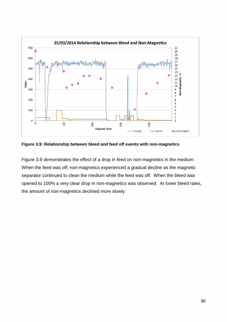
96

Figure 3.9: Relationship between bleed and feed off events with non-magnetics

Figure 3.9 demonstrates the effect of a drop in feed on non-magnetics in the medium.

When the feed was off, non-magnetics experienced a gradual decline as the magnetic

separator continued to clean the medium while the feed was off. When the bleed was

opened to 100% a very clear drop in non-magnetics was observed. At lower bleed rates,

the amount of non-magnetics declined more slowly.

97

Case D: The low density stability test:


correct medium samples at 10 min intervals for an hour and then add non-magnetics.

On 26/03/2014 the plant was operated at 1.30RD however, on observation, the medium

visually appeared to be stable. It is thought that this was due to the previous night shift

operating the plant at a target density of 1.6 and the higher levels of residual non-

magnetics in the system. In general the plant volumes were unstable on this day and it

was determined that it was not an ideal day to run this test. Observation of the desliming

spray test and the bleed operation and the effects on non-magnetics levels in the other

case tests (eg. 25/3/2014) demonstrated that non-magnetics can be quickly lost from a

system, but also quickly regained if the desliming sprays are turned off for a short period.

On this day, it can be seen that the level of non-magnetics in the circulating medium

responded well in the first test at 1.35RD, but after the density change at the 85 minute

mark, from 1.35RD to 1.30RD, the sump levels reached overflow (Figure 3.10a and

3.10b). Essentially, there was too much magnetite in the system and the plant did not

have a means of removing the excess. The non-magnetics did not respond as

significantly on the second occasion that the bleed was open, and in fact, went up after a

short drop. It was noted that the correct medium sump was overflowing to the dilute via

the floor sump part way through the second 100% bleed open test, which effectively meant

that the bleed was occurring via the overflow on the correct sump. In this situation,

operation of the bleed valve was ineffectual. As sump levels were already out of control in

the plant circuits it is not surprising that the level of non-magnetics in circulation didn’t

respond clearly to an opening of the bleed in the second test. Under a more controlled

sump level, it is expected that the outcome would have been different and that a more

pronounced drop in non-magnetics would have been evident. It is important to note that

this situation was a fairly extreme density change and the reasons for the plant sumps

overflowing primarily related to the design limitations of a plant without an overdense

storage system.

98

Figure 3.10a: Relationship between bleed and non-magnetics. When bleed was fully opened on two separate occasions on the same day, the level of non-magnetics dropped. The correct medium sump was full during the majority of the test work, however the drop in level can be seen when the bleed was initially opened fully. Figure 3.10b below shows the density and density set point during the same period.

Figure 3.10b: Relationship between density and %non-magnetics on the test day. The setpoint was dropped from 1.35 to 1.3 and non-magnetics remained relatively steady during the density change. This particular day was one where there had been a very high density setpoint of 1.6 overnight and the plant showed evidence of excess magnetite in the system.

99

Case E: Low density stability desliming sprays response test:


correct medium samples at 10 min intervals for an hour and then add non-magnetics to the

system by turning off the desliming sprays.

On 25th March, 2014 the desliming sprays were turned off, however the density setpoint

was high because of production requirements to operate at a higher density.

Nevertheless, a decision was made to proceed. During this period, there was no water

spraying on the desliming screen which meant that less of the fine material would pass

through the screen to the fines circuit. A proportion of the fine material, including non-

magnetics, instead overflowed the desliming screen into the coarse launder and then into

the wing tank. The desliming spray response test at New Acland revealed that the build

up of non-magnetics was rapid, however, the corresponding build-up of water in the dilute

circuit due to the spray water diverting across to the drain and rinse screens meant that it

was not feasible to continue. An increase in non-magnetics of 2.2% was observed after

the sprays had been turned off for two minutes (Figure 3.11). This increase was thought

to be due to the increase in fines entering the dense medium circuit. The desliming spray

water entered the dilute via the drain & rinse screen sprays and the dilute sump rose from

40% full to 100% full and overflowing within 2 minutes.

Figure 3.11: Desliming spray test period is marked by the vertical line. An increase in non-magnetics of 2.2% was observed after the change.

100

Test of using de-sliming sprays to control non-magnetics was abandoned after 2 minutes

due to the rapid water balance response for this particular plant. (Figure 3.11) Despite the

rapid response at New Acland, it is possible that some of the older plant designs may have

a slower water balance response. The author recalls seeing de-sliming screens running

without sprays on at other CHPP plants in the past. The results of this test suggest that

non-magnetic material from the de-sliming screen will rapidly improve non-magnetics

content in the medium, however, an alternative means of adding non-magnetics, such as

recycling a portion of thickener underflow or magnetic separator effluent may impact less

on the water balance.

101

Case F: Partition Testing and Determination of Residence Times for coarse particles in various sections of a DMC circuit:

Test: This case comprised two tests, both using cubic density tracers. A partition test

which compared standard 32mm tracers with 13mm RFID tracers was done. A residence

time test using a selection of radio frequency identification (RFID) tracers at various

densities to analyse times for coarse particles to travel through the various sections of the

DMC circuit was also completed on two separate test dates.

The Partition Tests

Figure 3.12 below demonstrates the normal route for a coarse coal particle travelling

through the DMC circuit.

Concentrate

Correct Medium

Wing Tank

Desliming

Reject

Product Product

Feed Weightometer

DMC

B

Figure 3.12: Normal route for coal particles.

Tracers are dispensed at the desliming screen and flow into the coarse launder. The tracer particles then enter the wing tank with the coal and are pumped to the DMC which then outflows onto the three drain and rinse screens where they are detected, or in the case of standard tracers, are manually collected.

102

For the two test days, tracers were dispensed at the de-sliming screen and detected at the

product and reject drain and rinse screens using a fixed antenna on the coarse launder of

each screen. As each RFID tracer had a unique identifier number, the travel time of each

individual particle as it travelled through the circuit could be measured. As tracer particles

also had a unique density, the partition curve could be determined for this route. Standard

density tracers were manually collected from the screens whereas the antennae on the

drain and rinse screens detected the RFID tracers. On both of the chosen test days, the

plant showed good stability with a differential calculated to be 0.21 on the first day, and

0.20 on the second test day. A differential below 0.4 would suggest that surging or

retention in the DMC was highly unlikely to occur. This was confirmed when it was

observed during the test that no retained particles were retrieved at the end of the test.

Figures 3.13 and 3.14 below show the percent (dry w/w) non-magnetics in the medium on

the test days. This was measured by comparing the relative masses of dried magnetics

and non-magnetics (expressed as a percentage) after running through a Davis Tube. This

indicates that the level of non-magnetics was at a sufficient level to avoid retention and did

not vary widely during the test.

Figure 3.13: % Non-magnetics (by weight) in the correct medium samples taken during the first day of tracer testing (Test 1) 24/10/2013 (Scott et.al. 2015)

103

Figure 3.14: %Non-magnetics (by weight) in the correct medium samples taken during the second day of testing at New Acland. (Test 2) 7th April 2016 (O’Brien 2016).

Non-magnetics levels were higher on this day, possibly due to a high rejects loading but the differential was only slightly lower than for the first test day.

Yields between the two test days were quite different. The first test had a yield of 45%

whereas the second test had a yield of 30%. The low second test yield created a high

degree of difficulty with recovering standard tracers from the reject screen due to a high

bed depth of over 100mm. The RFID tracers by comparison, were recoverable in higher

numbers during the second test as the antennae were able to detect tracers in spite of the

high bed depth. Partition curves were produced for the route from the desliming screen to

the drain and rinse screens. A discussion of the first test was also given in Scott et.al.

(2015). Both types of tracers were dispensed side by side onto the de-sliming screen and

tracers were collected on the two product drain and rinse screens and on the reject drain

and rinse screen. In the collection launders at the end of the drain and rinse screen,

Partition Enterprises placed RFID antennas to count individually labelled 13mm RFID

Tracers. The expectation from this partition test comparison of different sized tracers was

that results from both tests would be relatively similar for the given sets of plant conditions,

with the 13mm cut point being higher than the 32mm cutpoint. Tables 3.3 and 3.4 show

the recoveries for the standard tracers.

104

Table 3.3: Standard 32mm Tracer Results Test 1

Number of

Tracers

Tracer Density

Collected on

Product Screen

Collected on Reject

Screen

Missed Recovered Proportion to Product

Proportion to Reject

30 1.41 29 0 1 29 100 0

30 1.43 28 0 2 28 100.0 0.0

30 1.45 28 0 2 28 100.0 0.0

30 1.47 28 0 2 28 100.0 0.0

30 1.49 28 0 2 28 100.0 0.0

30 1.5 30 0 0 30 100.0 0.0

30 1.51 29 0 1 29 100.0 0.0

30 1.52 30 0 0 30 100.0 0.0

30 1.53 28 0 2 28 100.0 0.0

30 1.54 28 0 2 28 100.0 0.0

30 1.55 30 0 0 30 100.0 0.0

30 1.56 22 4 4 26 84.6 15.4

30 1.57 16 13 1 29 55.2 44.8

30 1.58 4 22 4 26 15.4 84.6

30 1.59 0 30 0 30 0.0 100.0

30 1.6 0 29 1 29 0.0 100.0

30 1.62 0 27 3 27 0.0 100.0

30 1.64 0 24 6 24 0.0 100.0

30 1.66 0 30 0 30 0.0 100.0

30 1.68 0 27 3 27 0.0 100.0

30 1.77 0 24 6 24 0.0 100.0

Table 3.4: Standard 32mm Tracer Results Test 2

Number of

32mm Tracers

Tracer Density

Collected on

Product Screen

Collected on Reject

Screen



30 1.32 30 0 0 30 100.0 0.0

30 1.35 30 0 0 30 100.0 0.0

30 1.40 28 0 2 28 100.0 0.0

30 1.41 29 1 0 30 96.7 3.3

30 1.42 25 4 1 29 86.2 13.8

30 1.43 21 7 2 28 75.0 25.0

30 1.44 17 11 2 28 60.7 39.3

30 1.45 5 23 2 28 17.9 82.1

30 1.46 0 27 3 27 0.0 100.0

30 1.47 0 26 4 26 0.0 100.0

30 1.48 0 20 10 20 0.0 100.0

30 1.49 0 22 8 22 0.0 100.0

30 1.50 0 25 5 25 0.0 100.0

30 1.55 0 25 5 25 0.0 100.0

30 1.59 0 25 5 25 0.0 100.0

105

The 13mm RFID tracers had recoveries that were relatively low in Test 1. Approximately

60% of tracers were recovered or detected. Interference due to the close proximity of the

screens influenced this result. Care was taken during set up of the second test to avoid

interference and hence recoveries were considerably improved in spite of the higher bed

depth. The problem of interference was remedied in the second test run and recovery

time was also lengthened to allow for slower travelling tracers to be recovered.

Consequently, the second test run had significantly better recovery rates for the 13mm

tracers. (Table 3.5 and 3.6)

Table 3.5: Results of 13mm RFID Tracer test 1

Number of

Tracers

Tracer Density

Collected on Product

Screen

Collected on Reject

Screen



30 1.32 17 0 13 17 100 0

30 1.48 22 0 8 22 100.0 0.0

30 1.49 23 0 7 23 100.0 0.0

30 1.5 17 1 12 18 94.4 5.6

30 1.51 22 0 8 22 100.0 0.0

30 1.52 19 2 9 21 90.5 9.5

30 1.53 18 3 9 21 85.7 14.3

30 1.54 11 9 10 20 55.0 45.0

30 1.55 7 12 11 19 36.8 63.2

30 1.56 3 17 10 20 15.0 85.0

30 1.57 5 14 11 19 26.3 73.7

30 1.58 0 20 10 20 0.0 100.0

30 1.59 2 19 9 21 9.5 90.5

30 2 0 18 12 18 0.0 100.0

106

Table 3.6: Results of 13mm RFID Tracer test 2

Number

of

Tracers

Tracer

Density

Collected

on Product

Screen

Collected

on Reject

Screen

Missed Recovered Proportion

to Product

Proportion

to Reject

30 1.3 28 1 1 29 96.6 3.4

30 1.32 28 2 0 30 93.3 6.7

30 1.35 27 3 0 30 90.0 10.0

30 1.38 24 6 0 30 80.0 20.0

30 1.40 23 7 0 30 76.7 23.3

30 1.41 18 11 1 29 62.1 37.9

30 1.42 12 17 1 29 41.4 58.6

30 1.43 5 24 1 29 17.2 82.8

30 1.44 3 25 2 28 10.7 89.3

30 1.45 0 29 1 29 0.0 100.0

30 1.46 0 30 0 30 0.0 100.0

30 1.47 0 28 2 28 0.0 100.0

30 1.48 1 27 2 28 3.6 96.4

30 1.49 0 30 0 30 0.0 100.0

30 1.50 0 30 0 30 0.0 100.0

30 1.59 0 30 0 30 0.0 100.0

Results of the standard 32mm tracer tests indicated that the cut point of the cyclone was

operating higher than for the 13mm RFID tracers. This was an unexpected result. Figure

3.15 is a graph of both partition curves showing the discrepancy in results. A comparison

of cut point is given in table (Table 3.7)

Table 3.7: Comparison of cut point and Ep for the 13mm and 32mm tracers in both tests.

Test 1 RD50 Ep

Test 2 RD50 Ep

13mm 1.55 0.013

13mm 1.419 0.021

32mm 1.57 0.007

32mm 1.44 0.007

107

Figure 3.15: A comparison of the tracer tests for 13mm and 32mm tracers on the two test days.

A cut point difference was noted on both occasions with the 13mm tracers demonstrating a lower cut point than the 32mm tracers.

108

The low detection rate of the 13mm RFID tracers in Test 1 and the relatively low

recoveries for the standard 32mm tracers were not ideal, but were sufficient for reliable

determinations of cutpoint and Ep values. Results of the standard 32mm tracer test 1

indicated that the cut point of the cyclone was operating close to 1.57 when measured

using the 32mm tracers and around 1.55 with the 13mm RFID tracers. The estimated Ep

was 0.007 for the 32mm versus 0.013 for the 13mm tracers. The partition curve for the

RFID tracer Test 2 suggested that the Ep of 0.021 was unusually high and that the cut

point was 1.419. This could have been due to the fact that the DMC body was well worn

and yields were low. The partition curve for the Standard 32mm tracers suggested that

the Ep of 0.007 was similar to the previous testwork. The cut point for the Standard 32mm

tracers was calculated to be 1.44. This again demonstrated that there was a cut point

difference between the 13mm RFID tracers and the 32mm standard tracers. The

difference in cut point would normally be expected to be higher for the smaller particles

than the larger particles, however in this case, the cut point for the smaller particles was

lower. This confirms that the same effect was visible in both tests.

Discussion of Partition Testing:

Possible reasons for the cut point reversal have been proposed by others, most notably

Wood (1990). He observed a number of cases which did not exhibit the usual progressive

increase of cutpoint with decreasing particle size. In these cases, the lowest cutpoint was

for an intermediate size fraction such as -8mm by +4mm. In those instances, cutpoints for

coarser coal or for 32mm tracers were slightly higher. Wood (in Crowden et.al. 2014)

conjectured reasons for this relating to porosity of coal and absorption of float sink

chemicals, however in the case of density tracers, no chemicals are required. Another

reason suggested by Wood was that there could be more resistance to large particles

flowing into the vortex finder where annular depth of slurry may be only 20mm and that this

could pose more of a challenge than the ease of exit via the apex of the cyclone.

Tracers used in previous research by I.A. Scott, (1988) were found to be differently shaped

to the tracers used in standard density tracer testing in coal plants. The tracers used by

Scott were flat, shale-like particles, rough shaped and appeared to have been put through

a crusher. The majority of particles were wide but flat in shape, which could have led to

109

differences in their behaviour in a DMC. This may suggest that particle shape could have

had a role to play in determining the cut points of the particles, however drawing firm

conclusions would require further work.

Prediction of residence times in a coal preparation plant.

The new design of RFID density tracers enabled a novel method to be used to determine

particle residence times in various parts of the DMC circuit. The method involved timing

RFID tracers passing through the circuit both during partition testing and also when

inserting into other parts of the circuit. The RFID density tracers were inserted in the

following locations (Figure 3.16):

• plant feed weightometer

• crusher feed at the end of the feed conveyor

• de-sliming water sump which feeds the de-sliming wing tank under the crusher

• de-sliming screen coarse launder (used for the partition testing)

• DMC outlets

• drain and rinse screen under-pans

• magnetic separator concentrate

• wing tank overflow

Other routes chosen for the RFID tracers were not used for producing partition curves due

to the relatively lower number of densities and tracers used. The number of insertion

points were changed slightly for the second day of testing in order to gain more information

about the medium circuit. The insertion points at the DMC overflow and underflow were

removed from the second test and additional tracers were instead added at the crusher

feed, the desliming water sump and the wing tank overflow. A summary of the residence

times through various parts of the circuits are given in table 3.8

110

Concentrate

Correct Medium

Wing Tank

Dilute

Desliming


Water

Bleed


Effluent

DMC


Gauge

Figure 3.16: The DMC circuit and the associated feed and collection points for the tracers in the Residence time tests.

Red dots denote tracer insertion points and green dots denote RFID tracer detection antenna locations

111

Table 3.8: A summary of the residence times through various parts of the circuits.

(Times are in mm:ss format)

Test Residence time From Residence time to Average Min Max

A Desliming Screen Drain & Rinse Screen 01:01 00:36 02:11

B DMC Overflow / Underflow Drain & Rinse Screen 00:20 00:15 00:26

C&D Drain Underpan Drain & Rinse Screen 02:36 00:43 29:06

E Feed Weigher Drain & Rinse Screen 02:25 02:00 03:27

F Mag Separator Concentrate Drain & Rinse Screen 09:50 01:10 39:36

G Deslime Water Sump Drain & Rinse Screen 08:37 02:09 35:51

H Crusher Feed Drain & Rinse Screen 01:55 01:36 02:25

I Wing Tank Overflow (to CM) Drain & Rinse Screen 06:53 01:23 31:48

The summary of residence times was used to estimate delays in the various parts of the

circuit in the dynamic model. As can be seen in table 3.8, particles that were inserted into

one piece of equipment did not necessarily take the same time to travel through the

system. The broad range of times for each test suggested that the data was multi-modal

and that some particles took different routes or settled out during transit. A discussion on

standard deviation is detailed in Appendix 5. The test ran for 40 minutes in total after

which any remaining particles that had not yet passed the antennae were considered lost.

Recovery rates were high, however it is believed that some particles could still have been

in transit at the 40 minute cut-off time. Further discussion of the routes taken is outlined

below, however for the purposes of dynamic modelling, the above table was sufficient for

use in the model to input delays. Table 3.9 is the model delay table. Consideration has

been made to the multiple routes possible within the DMC circuit and to some extent the

delays can be adjusted within a range. In many cases, the shortest particle residence time

was taken to ensure that the particle had not taken multiple routes of the system before

being detected.

112

Table 3.9: Delays used in the Dynamic Model (seconds)

Delay Description Delay time (s)

Bleedsplit_delta Dead time from correct sump to bleed valve 15

Deslime_delta Dead time from bleed valve to deslime 7

Wing_delta Dead time from deslime to wing tank 6

DMC_delta Dead time from feed to DMC 15

Drain_delta Dead time from combined drain to wing tank 12

Rinse_delta Dead time from combined rinse to wing tank 12

from_Dil_delta Dead time from dilute sump to mag seps 28

MSCon_delta Dead time from mag sep cons to correct sump 12

Bleed_delta Dead time from bleed valve to dilute sump 6

Tracer Routes

The following is a description of the possible routes that a tracer particle may take from

each entry point to its ultimate destination at the drain and rinse screen coarse launder.

Despite the normal route for coal particles being via the wing tank to the DMC, there are

circumstances where the coal does not follow this route, an example of this is rafting coal.

Inside the wing tank, the separation between the coal side and the seal leg side is via an

orifice plate. When rafting occurs in the wing tank, coal travels up through the orifice plate

into the seal leg of the wing tank, and then overflows instead of flowing down into the DMC

pump. Rafting occurs when there is an insufficient downward flow in the wing tank to

prevent low density coal particles from floating. If the orifice flow is reversed, then rafting

can occur up into the seal leg. As there is no oversize protection on the correct medium

sump, the coal particles are able to travel back to the desliming screen coarse launder or

travel into the dilute sump via the bleed valve on the correct medium line. The bleed valve

is a butterfly valve and although it may appear to be fully closed, operators have noted that

occasionally rafted coal particles can get stuck in the valve causing the valve to pass when

closed. The impact of coal particles in the dilute sump is that the magnetic separator may

see particles of larger size. A 20mm square mesh oversize protection exists on the

113

magnetic separator underpan, however particles travelling through the magnetic separator

underpan could still be of reasonable size to pass through the 20mm mesh. During the

RFID tracer tests, the bleed valve was closed during addition to the correct medium lines,

however, the time that some particles took to pass through the system was significantly

longer than expected. It is therefore quite possible that some of the 13mm RFID tracer

particles could have passed through the magnetic separator underpan, either due to a

bleed valve that didn’t fully close despite reading 0% open on the control room screen, or

alternatively, due to the bleed being opened too early after the test. In general the bleed

was closed for approximately five minutes. Based on the previous test work, this seemed

to be a reasonable number to use. It was discovered in the second RFID tracer test,

however, that some particles can take considerably longer to exit the circuit. Figure 3.17

below shows possible alternate routes for coarse coal particles due to rafting.

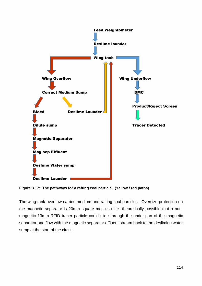
114

Feed Weightometer

Deslime launder

Wing tank

Wing Overflow Wing Underflow

Correct Medium Sump DMC

Product/Reject Screen

Bleed Deslime Launder

Dilute sump Tracer Detected

Magnetic Separator

Mag sep Effluent

Deslime Water sump

Deslime Launder

Figure 3.17: The pathways for a rafting coal particle. (Yellow / red paths)

The wing tank overflow carries medium and rafting coal particles. Oversize protection on

the magnetic separator is 20mm square mesh so it is theoretically possible that a non-

magnetic 13mm RFID tracer particle could slide through the under-pan of the magnetic

separator and flow with the magnetic separator effluent stream back to the desliming water

sump at the start of the circuit.

115

Concentrate

Correct Medium

Wing Tank

Dilute

Desliming

Reject

Product Product

Water

Bleed

Gauge


Effluent

Feed Weightometer

DMC

Figure 3.18: A pictorial view of the pathways for coal particles including rafting coal.

116

The pathway in which the medium travels through the DMC circuit is slightly different to

that of the normal coal particles. Figure 3.19 shows the possible pathways for the medium

to travel through the DMC circuit. The pathway of the medium also includes the dilute

circuit as a bleed from the correct medium line and the rinsed medium ensures that there

is a build-up of water in the system which needs to be removed via the magnetic

separators. The magnetic separators also strip non-magnetic material out of the system

via the dilute circuit.

Correct Medium Sump

Wing Overflow

Deslime launder

Wing tank Bleed

Wing Underflow Dilute sump

DMC

Drained Medium Magnetic Separator

Product/Reject Screen Rinsed Medium

Mag separator Concentrate

Coarse Product

Figure 3.19: Possible routes for the medium.

The medium that follows the coal pathway will travel to the desliming screen coarse

launder from the correct medium sump. It then passes through the wing tank and enters

the DMC feed pump. Once through the DMC, the medium splits onto product and reject

drain and rinse screens and a proportion of the medium will drain through, remaining

medium will either wash through to the rinse underpan or carry over into the coarse

launder with the product. The return drain medium enters the wing tank seal leg where

either it passes through the orifice plate in the wing tank and follows the coal pathway, or it

overflows into the correct sump. From the correct sump, medium is either diverted to the

bleed line across to the dilute sump or is pumped to the desliming screen coarse launder.

The return rinse medium flows to the dilute sump and is processed via the magnetic

separator which returns concentrate directly into the correct medium sump.

117

For the residence time tracer test work, each RFID tracer had a unique identification label.

Times were able to be tracked for each individual tracer and then compiled into a

summarised data set. Below is a detailed analysis of individual circuits within the plant. In

some cases only small quantities of RFID tracers were detected. The data was however

sufficient to give an indication of times taken for coarse particles to travel through the

circuit. Of particular interest also is the data which varies widely between individual

particles which indicates that some particles may have travelled a different path to others.

The multi-modal nature of the distributions suggested that there was little value in

measuring standard deviations as it was difficult to determine exactly which route the

particle took. What was clear, was that there was not one data set, but multiple sets of

data for a specific insertion point. The travel time depended on the amount of time the

particles settled out in the system, or the number of times that the particles circulated in

the medium before joining the coal stream at the wing tank.

Desliming Screen to Drain and Rinse Screens

Test A was the route followed for the conventional tracer testwork and was done

concurrently with the standard tracers. Tracers were dropped into the circuit at the

desliming screen and travelled into the DMC wing tank. They were then pumped through

the DMC and detected on the product and reject drain and rinse screens. Table 3.10

Table 3.10: Tracer times from de-sliming screen to drain and rinse screen oversize for both days of the testwork


A Desliming Screen Drain & Rinse Product 1 00:57 00:37 01:41

Desliming Screen Drain & Rinse Product 2 01:00 00:36 01:56

Desliming Screen Drain & Rinse Rejects 01:02 00:43 02:11

Desliming Screen Drain & Rinse Overall 01:01 00:36 02:11

When data from test A was compared by density, the following graph (Fig 3.20) was

generated. Attempts to identify a trend in the data indicated that there was very low linear

correlation of the density of the particles against the time taken to pass through the circuit.

It is important to note however, that this data was collected only for particles travelling

118

between the desliming screen and the drain and rinse screens with virtually no opportunity

for hold-up in the system apart from the possibility of rafting in the wing tank. It is thought

that rafting was unlikely to have occurred on the two test days as the density target was

not significantly high. Process operators have commented that rafting usually occurs

when targeting a high density of over 1.60RD.

The correlation between density and travel time was low for this short route, which

suggests that density does not have a strong influence on travel time for the coal through

the DMC circuit. Relative travel times of particles in the medium recovery circuit are

discussed later.

Figure 3.20: Relative transit times for different density particles to travel from the desliming screen to the drain and rinse screen coarse launders. This data is combined from both of the test days.

From the above table and figure 3.20, it can reasonably be concluded that when there is a

single, short route to be taken through the circuit with a low chance of segregation of

particles in vessels, there is not a density effect on residence time.

119

DMC overflow and underflow to the Drain and Rinse Screens This test involved dispensing tracers at the outlets of the DMC and collecting them on the

drain and rinse screens. Tracers travelled only a small distance, but this test gave an

indication of how long it took for a coal particle to travel down the screen. (Table 3.11)

Table 3.11: Tracer times from DMC outlets to the drain and rinse screen oversize


B DMC Overflow/Underflow Drain & Rinse Screen 00:20 00:15 00:26

Drain underpans to the Drain and Rinse Screens

This test involved dispensing tracers into the correct medium (drain) side of the drain and

rinse underpans and collecting them on the drain and rinse screen oversize. Particles

travelled through the seal leg side of the wing tank and then either joined the DMC feed or

overflowed into the correct medium sump. The results of this test showed a broad scatter

indicating that some tracer particles took a different route through the circuit. (Table 3.12).

Table 3.12: Tracer times for travel from drain and rinse underpan (drain side) to the drain and rinse screen oversize.


C&D Drain underpan Drain and Rinse Screen 02:36 00:43 29:06

Closer inspection of the results indicated that density did not necessarily determine the

residence time of the tracer particles. In one case, two particles of identical density of 1.34

took vastly different times to reach the end point. (Figure 3.21) This suggests that DMC

retention was not to blame for the slower particle arrival. A possible reason was that the

slower tracer could have overflowed from the wing tank seal leg into the correct medium

sump and then returned to the de-sliming screen before being pumped back to the DMC

via the wing tank. However, a more plausible explanation in this particular case is that

there was observed silting of magnetite occurring in the drain and rinse screen under-pan,

and that dispensing tracers into the side edge of the under-pan may have resulted in a

slower transit due to the silt build up. In hindsight, the better location for dispensing the

tracers would have been to find the exit point for the drain, however the difficulty of access

to the under-pan made this particular test difficult under any circumstances. There is

120

insufficient data to draw a concrete conclusion that density does not have an effect for this

particular part of the test, it does, however, give an indication of possible pathways that a

particle may take.

Figure 3.21: Individual RFID Tracer results for travel to the various drain and rinse screens from the drain side underpans

In the case of the particles of higher densities (around 2.00), the times to reach the drain

and rinse screen were considerably more consistent, suggesting that the pathway of the

heavier particles was less interrupted. This test was, however, deemed unreliable due to

the silting in the underpan.

Feed belt weightometer to drain and rinse screens

This test involved inserting tracers at the feed belt weightometer and collecting them on

the drain and rinse screens. The tracers travelled the full length of the plant, passing

through the secondary and tertiary crushers into a feed sump and then onto the desliming

screen. The tracers then entered the DMC circuit travelling with the coal, and were

collected on the drain and rinse screens as per the other tests. This test gave an

121

indication of the time taken for a change to be registered on the weightometer and the time

taken for the plant to respond. (Table 3.13)

Table 3.13: Timings from the feed belt weightometer to the drain and rinse screens


E Feed Weigher Drain and Rinse Screen 02:25 02:00 03:27

The average time for tracer particles to reach the drain and rinse screens from the

weightometer was 2 minutes, 25 seconds. This indicated that despite particles travelling

through a minimum of three sumps and a sizing station during their journey, they were still

relatively consistent in the time taken to reach the end of the screens. It also suggests that

coal particles do not have a long residence time in the plant. (Figure 3.22)

Figure 3.22: Tracer particle times from the feed belt weightometer to the drain and rinse screens via the DMC circuit.

122

Magnetic Separator concentrate to the Drain and Rinse Screens

This test involved inserting the tracers at the magnetic separator concentrate product side

and detecting the tracers at the drain and rinse screens. The shortest time for a tracer to

flow from the magnetic separator to the drain and rinse screens was 70 seconds. This

suggests that the particle travelled directly into the correct medium pump and flowed to the

wing tank without any detours. This data point gives a useful measure of delay time for

this section of the circuit. (Table 3.14) Figure 3.23 shows that some particles took

considerably longer to exit the circuit, with some taking up to 39 minutes to circulate. It is

possible that the 39 minute particle could have taken several trips around the circuit or it

could have settled out somewhere before being dislodged. From the data it is not possible

to know which of these possibilities occurred.

Table 3.14 Residence times for particles leaving the magnetic separator and travelling to the drain and rinse screens.


F Magnetic Separator Drain and Rinse Screen 09:50 01:10 39:36

Figure 3.23: Particle tracer time vs. Tracer density for particles travelling to the Drain and Rinse Screens from the concentrate launder of the magnetic separator

123

Desliming Water Make-up Sump to the Drain and Rinse Screens

This test involved inserting the tracers at the desliming water make-up sump which exists

under the secondary sizing station. Water from this sump is pumped into the desliming

wing tank (desliming screen feed sump) and mixes with the sized raw coal before being

pumped to the desliming screen. This sump is significant as effluent from the magnetic

separator is pumped to this location and coarser particles will re-enter the DMC circuit via

the desliming screen. Results of this test indicated that the average particle took over 8

minutes to transfer through the DMC circuit from this location, and some took up to 35

minutes. (Table 3.15) The long lead time is a possible reason why some tracers were not

recovered after 40 mins. If particles travelled across to the dilute sump via the bleed, they

would likely have travelled in the magnetic separator effluent stream back to the de-sliming

water sump, thereby greatly extending their time in the circuit. In the de-sliming water

sump, where the slurry is mostly diluted to water, the densest particles took the longest

amount of time to travel through the system (Figure 3.24). This makes sense given that a

particle with a density around 2.00 would normally sink in water. It is possible that the

denser particles could have settled quickly to the bottom of the de-sliming sump before

eventually being stirred up by mixing action.

Table 3.15 Residence times for particles leaving the Desliming water make-up sump and travelling to the drain and rinse screens.


G Deslime Water Sump Drain and Rinse Screen 08:37 02:09 35:51

124

Figure 3.24 Particle residence time vs. Tracer density for particles travelling to the Drain and Rinse Screens from the Desliming Water Make-up Sump.

Crusher feed to the Drain and Rinse Screens This test involved inserting the tracers at the feed to the secondary sizing station before

the plant. The coal from this point enters the de-sliming wing tank and is pumped to the

de-sliming screen where it follows the coal through the DMC circuit. Times for particles to

travel through this circuit were consistently under two and a half minutes, suggesting that

no particles took alternate routes through the plant. (Table 3.16 and Figure 3.25)

Table 3.16: Tracer times for travel from the feed to the secondary crusher/sizer to the drain and rinse screen oversize.


H Crusher Feed Drain and Rinse Screen 01:55 01:36 02:25

125

Figure 3.25: Particle residence time vs. Tracer density for particles travelling from the crusher feed to the drain and rinse screens.

Wing Tank Overflow to the Drain and Rinse Screens

This test involved inserting the tracers at the overflow exit of the wing tank where it travels

into the correct medium sump. This was intended to give an indication of time in the

correct medium sump. Times varied widely and from this, it can be concluded that the

medium circuit residence times can be considerably longer than the coarse coal travel

path. Particles taking 1 minute 23 seconds to exit the circuit are assumed to have entered

the correct medium pump very shortly after being dropped into the overflow, and then were

pumped directly to the DMC wing tank. (Table 3.17) Particles which took a longer period

of time could have settled out in the correct medium sump, or have been pumped via the

bleed across to the dilute circuit before eventually re-entering the circuit with the raw coal

at the de-sliming screen. (Figure 3.26) Interestingly, particles of all densities took the short

route, but only the heaviest and lightest density particles took the longer periods of time to

exit the circuit.

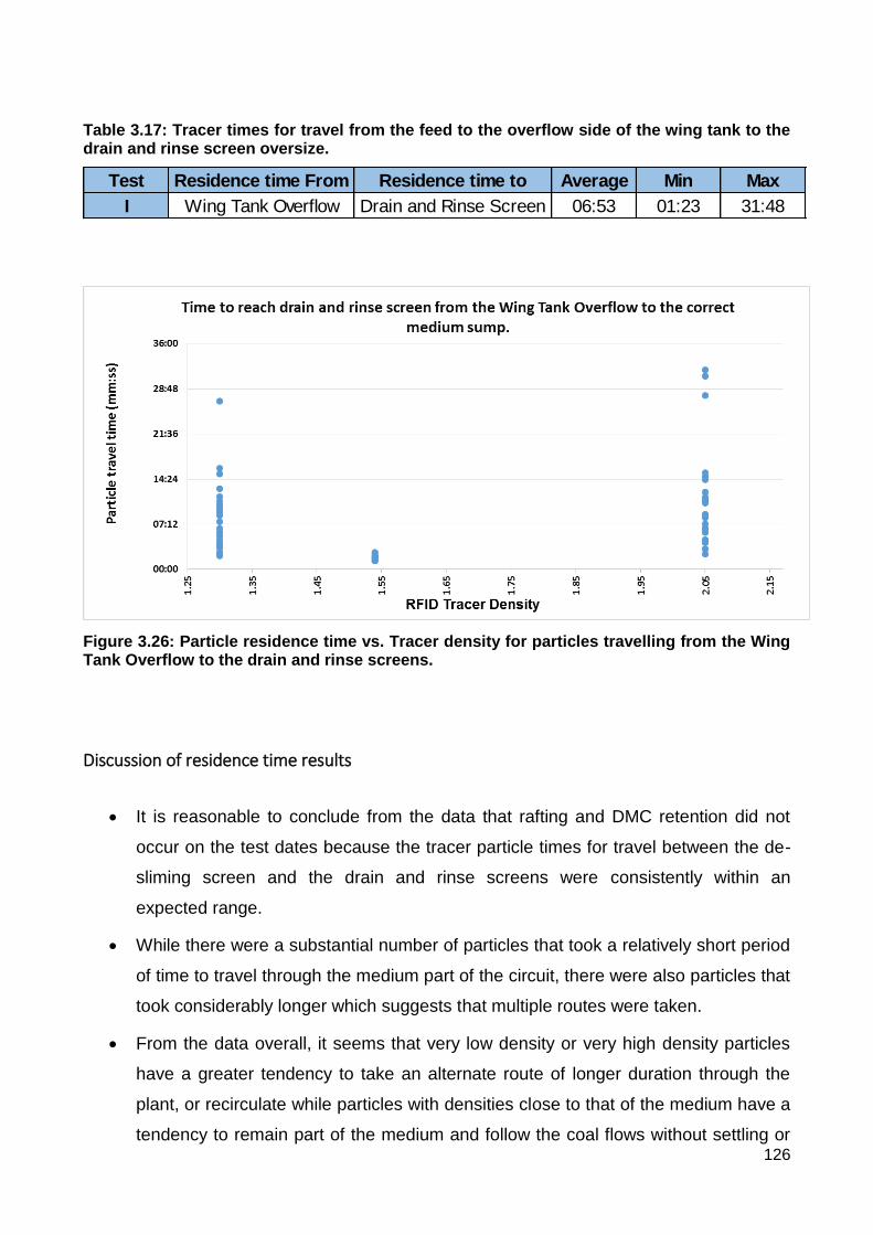
126

Table 3.17: Tracer times for travel from the feed to the overflow side of the wing tank to the drain and rinse screen oversize.


I Wing Tank Overflow Drain and Rinse Screen 06:53 01:23 31:48

Figure 3.26: Particle residence time vs. Tracer density for particles travelling from the Wing Tank Overflow to the drain and rinse screens.

Discussion of residence time results

It is reasonable to conclude from the data that rafting and DMC retention did not

occur on the test dates because the tracer particle times for travel between the de-

sliming screen and the drain and rinse screens were consistently within an

expected range.

While there were a substantial number of particles that took a relatively short period

of time to travel through the medium part of the circuit, there were also particles that

took considerably longer which suggests that multiple routes were taken.

From the data overall, it seems that very low density or very high density particles

have a greater tendency to take an alternate route of longer duration through the

plant, or recirculate while particles with densities close to that of the medium have a

tendency to remain part of the medium and follow the coal flows without settling or

127

floating. An explanation of medium flow observations from the above residence

time tests is proposed in Reason 1 and 2 below.

Reason 1: Lighter particles floating into the bleed stream

o The design of the bleed line which branches off from the main correct

medium line may be a cause of segregation of the medium. The main

correct medium line is horizontal just after a right angled bend and then the

bleed line runs vertically upwards from the top of the correct medium line.

There is an opportunity for particles to begin to settle in the horizontal plane

before reaching the bleed line. Particles of lighter density could have an

increased tendency to migrate up into the bleed line whereas heavier

particles would be more inclined to flow along the bottom of the horizontal

pipe.

Reason 2: Silting in the Correct Medium sump and in underpans.

o The explanation of why heavier particles might take longer to arrive at their

destination is thought to be due to build-up of heavier particles, or “silting” of

material in the correct medium sump and in the underpans of the drain and

rinse screens. As the correct medium sump operates at a higher density

than the medium measured at the nucleonic gauge, and has no mechanical

agitation, it is proposed that the multiple streams of higher density magnetite

entering the sump create flow interruptions in the sump leading to a silting up

of material in the sump.

128

3.4 Experimental work Conclusions

The experimental work conducted as part of this PhD Thesis is a sub-component of an

ongoing body of research by CSIRO and the University of Queensland (JKMRC). Analysis

of non-magnetics concentration and other sampling and data collection was done in

parallel with this test work. Plant observations and regular interactions with CHPP

personnel have provided unique insights into the operation of the DMC circuit under

varying conditions. The comparisons of density tracers of two different particle sizes has

provided an interesting comparison of cut point. In the partition tests, the expectation of

smaller particles being of higher cut point did not occur. The density tracers were then

used in a new experiment to determine residence times of individual particles in the DMC

circuit. This data has enabled realistic delays to be determined for use in the dynamic

model. The experimental work completed has highlighted that there are still further areas

to investigate in relation to particle and medium behaviour in a DMC circuit. The findings

of the experimental work are summarised below:

Summary of Experimental Work Findings

Case A: Good density change

After a density increase during stable operation, the level of non-magnetics was

found to reduce with an increase in correct medium bled to the dilute circuit.

A feed off event which occurred during the trial demonstrated a rapid loss of non-

magnetics from the medium, suggesting that the amount of non-magnetics in the

coarse coal circuit is strongly affected by the feed.

Despite a low differential (stable medium) and a carefully orchestrated good density

change, the medium took over an hour to recover back to the level of non-

magnetics before the density change.

Case B: Unstable Volume

When operating at a high level in the correct medium sump, and at a low density set

point, the plant demonstrated difficulty in maintaining a sufficiently low density due

to excess magnetite. This suggested that an alternative means of removing

129

concentrated magnetite such as an over-dense or magnetite pit return line was

needed as an alternative to returning magnetite to the correct medium sump.

When the correct medium sump and the dilute sump were in an overflow situation,

the level of non-magnetics also became difficult to control. An initial drop in non-

magnetics was noticed upon opening of the bleed to 100%, and a slight recovery of

non-magnetics was noted when the bleed was closed down to 20%.

In a situation of unstable volume, it is difficult for the plant operator to achieve stable

density operation. Volume control becomes a predominant issue at the expense of

non-magnetics and density control.

Case C: Stepwise density change

A step-wise density change resulted in a slower density response when compared

with a single change in density.

The level of non-magnetics dropped markedly when the feed was left off for an

extended period of time. Density also dropped.

The level of non-magnetics dropped when the bleed was opened, and began rising

when the bleed was closed.

After start up, the level of non-magnetics took over 60 minutes to return to prior

levels despite operating on a high relative density.

Time taken to reach density was slower when the amount of non-magnetics was

low and the plant feed had been off for a considerable time. Yield losses were

estimated at 17% over 11 minutes.

Case D: Low density stability

Non-magnetics levels did not respond as well when sumps were in an overflow

situation, however a drop in non-magnetics was noticeable when the bleed was

opened.

Stability at low density was impacted by volume control due to excess magnetite.

Due to the fact that the plant had run at very high density just prior to the low

density change, the medium was very stable on the test date and no surging events

occurred.

Case E: Desliming sprays response test

Closing the desliming sprays had the effect of rapidly increasing the level of non-

magnetics in the medium.

130

The rate of build-up of non-magnetics was 2% over 2 minutes.

The use of desliming sprays to control non-magnetics was not feasible for this

particular plant design due to the sensitivity of the water balance, however the

concept may work for other designs.

Ultimately another means of adding non-magnetics to the medium such as

thickener underflow may need to be investigated.

Case F: Tracer Testing

The prediction of cut point for different sized tracer particles showed an unusual cut

point reversal between the 13mm RFID and 32mm standard tracers. This was

observed on three separate occasions and it was concluded that the effect was

real. The observations were also confirmed when a literature review of a thesis by

Wood (1990) demonstrated similar effects. It was also determined that the original

cause postulated by Wood was incorrect as no float sink chemicals were present in

the case of the tracer tests at New Acland, therefore eliminating chemical

absorption as a possible cause. Other possible reasons could relate to DMC

geometry or particle shape, but more testwork would be needed to determine other

causes.

RFID residence time testing of coal particles travelling through the dense medium

yielded valuable information on time delays within the circuit and assisted with

model development.

Times measured for tracers to travel through the DMC circuit were surprisingly

short, with the times from the desliming screen through the DMC to the drain and

rinse screens ranging from thirty-six seconds to just over two minutes. There was

no significant difference based on the density of the coal particle for this pathway

and rafting and DMC retention were not evident.

The time for a coal particle to travel from the weightometer to the drain and rinse

screens ranged between two minutes and three and a half minutes. This

highlighted the rapid response of the circuit to changes in feed.

A density effect was noticed for particles travelling in the medium streams. The time

taken for particles to travel through the medium differed for denser tracers when

compared with low-density particles and with particles of near gravity. This was

concluded to be the result of settling out of some of the heavier particles from the

131

medium, and floating of some of the low density particles up into the bleed stream.

Particles that were close to the cut point had a strong tendency to flow as part of the

medium and not segregate out, resulting in shorter time travel.

132

4. Development of the New Acland DMC Circuit Dynamic Model

4.1 Introduction

For many years, steady state models have been used in process plant design. These

simplified models have sufficed for developing capacity constraints for a coal handling and

preparation plant. Designers then relied upon bore core data, commissioning

measurements and process control instrumentation to ensure that the built processing

plant operated within the design parameters established in the steady state models. The

disadvantage of a steady state model is that cases may arise where efficiency is lost

because of upsets in the plant that are undetectable unless tracked over time. For

example, a drop in wing tank level may lead to surging of the dense medium cyclone or

pumping inefficiencies that cause a short term loss of product into the rejects stream. In a

steady state model this case would be difficult to incorporate, however in a dynamic

model, time delays, and sump level effects are all included. Similarly, for components in a

stream that change due to continual changes in feed quality or particle distribution, it is not

easy to model as a steady state case other than with a basic mass balance. Dynamic

modelling is also particularly useful for analysing plant start-up or shut-down events where

delays may exist in the time it takes for material to reach each unit operation.

In the front end engineering design stage, a number of feeds or blended feeds are passed

through a steady state model to establish the extremities of the plant capacity

requirements and to predict yields. A plant that fluctuates from 15% fine coal in the feed to

40% fine coal in the feed would have a significant impact on the fines circuit in terms of

capacity, and this can be modelled by putting both cases through a steady state model.

This allows a snapshot in time to be analysed against other cases. Steady state systems

are applicable when a simplified system is required or when little change occurs over time.

A dynamic model, by comparison, is time-based, and has the capability to consider the

incremental effects on the circuits when the plant is running. A dynamic model can identify

opportunities for the control system to react faster and to alleviate plant upsets due to a

133

change in feed condition. The disadvantage of a dynamic model is that complexity can be

high and this often drives the choice of a simpler steady state model.

The development of the dynamic model for the New Acland site followed a number of

stages. LIMNTM and Microsoft Excel were initially used to create a steady state model of

the dense medium circuit. LIMN is widely used in the coal industry as well as in other

dense medium processes such as iron ore but is not capable of dynamic modelling at this

time, so the choice of dynamic modelling software was made on the basis of functionality

and compatibility with Microsoft Excel. Two options were considered in the software

selection process for a dynamic model. SysCADTM, a process flowsheet and modelling

software developed by Kenwalt, and MATLABTM, a mathematical programming software

developed by Mathworks. Early attempts to model in SysCAD indicated that considerable

customisation and work-arounds would be required, and although this software was well

supported, a decision was made to use Matlab which could be completely tailored for the

purpose.

Matlab is a mathematical programming language that utilises matrices and vectors to

shorten code length. Its power is derived from the ability to manipulate large arrays of

data in a few short lines of code. The program can combine functions, algorithms and

matrices, solve complex equations and simplify other code languages using matrices and

vectors. Matlab can also plot functions, create graphical user interfaces and interface with

programs written in other languages code including C, C++, Java, Fortran and Python.

The powerful toolboxes contained in Matlab-Simulink can be utilised for chemical

engineering applications such as process control and automation. The capability of Matlab

to take input tags from site equipment and upload data from excel spreadsheets is also

extremely useful. While Matlab is not an intuitive programming language, it was decided

that the functionality and potential to build in additional options into Matlab without the

need to go through a program development step through third party support was an

advantage.

4.2 Model Construction

The construction of the dynamic model began with a process of identification of the

empirical models to be used with each unit operation. During the process of model

134

development, regular visits were made to New Acland Plant to confirm specific piping and

design requirements for the model. Residence time information was also collected while

onsite for later use in dynamic modelling. The specific test work carried out using density

tracers is detailed in the Experimental Work chapter of this thesis. Calculations for

residence times from plant measurements were inputted as time delays in the dynamic

model. Where insufficient information existed, logical assumptions were made.

The inputs to the dynamic model consisted of four individual components: coal, water,

magnetite and non-magnetics. This was done so that each component could be traced

through each section of the circuit. The overall masses and volumes were also tallied at

each stage of the model so that each unit operation balanced. The basis used throughout

the model was volumetric flowrate, in cubic metres per second, with conversions to mass

flow rate as necessary to suit specific empirical models. The most current and widely used

DMC models were found in Crowden et.al. (2013). A Microsoft Excel mass balance of the

DMC circuit enabled basic flows to be tested and verified against plant data.

In general terms, a material balance comprises the following equation:

₌ - + -Accumulationor depletion within the

system

INPUTSTransport into the

system through the system boundary

OUTPUTSTransport out of

the system through the system

GENERATIONwithin the

system

CONSUMPTION within the

system

Fig 4.1: Material balance (Himmelblau 1989 eq.6.1,p628)

In the coal preparation case, the material balance could initially be assumed in terms of

gross tonnes or volume, and that no generation or consumption occurs. Although some

breakage of larger particles does occur in the coal preparation plant circuits, this may

initially be discounted for simplification. The equation was then simplified to:

₌ -Accumulationor depletion within the

system

INPUTSTransport into the

system through the system boundary

OUTPUTSTransport out of

the system through the system

Figure 4.2: Material balance excluding generation and consumption

135

The balance could then be increased in detail to include individual stream components,

namely magnetics, non-magnetics, coal and water. In practice, some breakdown of clays

and particle size degradation due to breakage does occur in the circuits. This breakage

has the effect of influencing the build-up of non-magnetics in the dense medium circuit.

On an individual component balance level, this could be taken into account if wet tumbled

coal data results and dry tumbled results were compared. As an alternative, a slimes

factor could be applied, where breakage is assumed as a percentage of the total based on

practical estimation from typical plant data. For this model, the ‘slimes factor’ method was

used. In addition to the slimes factor, a slimes fraction was added to account for the

proportion of non-magnetic slimes in the raw coal.

The Matlab dynamic simulation model was developed with a number of functions as

separate files feeding into the main script in Matlab. Figure 4.3 shows the design of the

Matlab simulation. The script also included global variables and these variables were

used by both the supporting functions and by commands in the main script. Due to their

multiple uses, they have been represented as a separate ring in figure 4.3, however, in

practice, they are integrated into the script and function files and are not a separate file in

themselves.

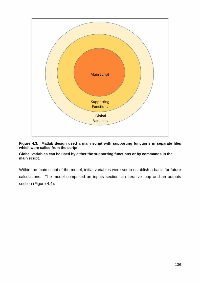
136

Main Script

SupportingFunctions

Global Variables

Figure 4.3: Matlab design used a main script with supporting functions in separate files which were called from the script.

Global variables can be used by either the supporting functions or by commands in the main script.

Within the main script of the model, initial variables were set to establish a basis for future

calculations. The model comprised an inputs section, an iterative loop and an outputs

section (Figure 4.4).

137

Figure 4.4: The dynamic model process flow

Empirical formulae for the unit operations were placed inside the loop. The loop

essentially consisted of an operator selected run-time length of which each iteration step

represented one second of plant time. The iterations stepped through for the length of the

run-time, each time recalculating the material balance inside each unit operation. This

design was based on the work of Askew (1983). Delays in the plant were represented as

a table of values from 1 to n where the new value replaced the first value in the table and

consequently displaced the nth value where the nth value is the total time of the delay.

(Figure 4.5)

1 2 3 4 5 6 7 ... n

Input Cell Output Cell

New Data

Data delayed by time 'n'

Figure 4.5: A visual representation of how the delays work in the model.

For example, for a delay of 15 seconds, the data will have to shift 15 spaces across (15

seconds). The delays in the plant were determined using RFID tracers and this is

described in the Experimental Work section. The output of the model took the format of

storage files used for plotting of trends of the data to view and ensure that the behaviour of

the components and unit operations were typical of real plant situations. Figure 4.6 shows

138

the empirical relationships used in the model for each unit operation within the DMC

circuit.

ITERATIVE LOOP

Desliming Screen (Whiten model)

INPUTS Correct Medium (Tank geometry) OUTPUTS

Plant Feed Wing Tank (Tank geometry) Product coal

Magnetite DMC (JKMRC-Wood Model) Coarse rejects

Water Coarse Product and Reject (JKMRC-Wood Model) Effluent

Drain and rinse Screens (Firth & O'Brien Model) Magnetite losses

Dilute & Floor sumps (Tank geometry) Non-magnetics losses

Magnetic Separators (Rayner model)

Figure 4.6: Model Architecture. The overall structure of the dynamic model is described in the above diagram.

The model outputs from each unit operation were checked using a “black box” method. In

this method, all items within each unit operation were considered to be inside a box, and

only input and output streams from that box were balanced. This was done for each unit

to verify that the model would balance. These individually tested unit operations were then

combined into the simulation model.

Once the overall mass balance and volume balances were established for each unit

operation in the DMC circuit, each stream was split into individual components of coal,

water, magnetite and non-magnetics. The non-magnetics was defined as fine clays and

small coal material that formed part of the medium and this was experimentally measured

using a Davis tube on samples of medium, and then weighing the dried samples of

magnetics and non-magnetics and obtaining a dry mass% split. Representation of

components was achieved using the format of a multicomponent vector [coal, water,

magnetite, non-magnetics, total-stream]. This multicomponent vector format was very

useful because it improved the ease of transfer of components through the unit operations

without the need to create dummy streams or to write separate equations for each

individual component, and it therefore considerably shortened the number of lines of code.

139

For the dynamic material balance, the time for material to reach one part of a circuit will

differ from another part of the circuit, and therefore, system delays need to be built into the

model. System delays were calculated as functions in MatlabTM. The residence times for

particles travelling through the circuit were measured using RFID tracers and were used

as inputs for the delay functions. The delays and their descriptions are detailed in table

4.1.

Table 4.1: A full list of the delays for the dense medium circuit are below:

Delay Description Delay time (s)

Bleedsplit_delta Dead time from correct sump to bleed valve 15

Deslime_delta Dead time from bleed valve to deslime 7

Wing_delta Dead time from deslime to wing tank 6

DMC_delta Dead time from feed to DMC 15

Drain_delta Dead time from combined drain to wing tank 12

Rinse_delta Dead time from combined rinse to wing tank 12

from_Dil_delta Dead time from dilute sump to mag seps 28

MSCon_delta Dead time from mag sep cons to correct sump 12

Bleed_delta Dead time from bleed valve to dilute sump 6

These delays formed part of the initial set up of the model before the first iteration. Initial

volumes in the sumps and initial process parameters were also scripted prior to the

iteration loop. These included setting density controls, wing tank, correct medium and

dilute sump levels, setting initial stream compositions, feed tonnage, drain and rinse

screen conditions, raw coal size distribution, washability data and desliming screen

partition to the coarse stream. The length of the simulation was given by the variable

sim_time, expressed in seconds. This variable was able to be changed to reflect longer or

shorter run times. The number of iterations was then simply set as i=1 to ‘sim_time’.

The size distribution used for the dynamic model testing was entered into the model script

as size_consist= [37, 18, 10, 6, 3, 1.4, .7, .46; 23.4, 43.1, 18.0, 8.6, 3.3 2.0, 0.8, 0.8];

This is represented in Table 4.2.

140

Table 4.2: Size Distribution

Size (mm) 37 18 10 6 3 1.4 0.7 0.46

Mass (g) 23.4 43.1 18.0 8.6 3.3 2.0 0.8 0.8

Washability data used for the model was uploaded as a separate .csv file. The washability

data used for the dynamic model testing is shown in Table 4.3 below. This washability

data can easily be replaced by renaming a new file in the same format:

Table 4.3: Washability data

Density Mass Ash

1.28 17.10 9.5

1.33 10.57 16.7

1.38 9.79 23.8

1.43 8.25 29.5

1.48 7.72 34.6

1.51 1.38 38.8

1.54 0.94 38.7

1.56 0.19 39.5

1.59 0.64 40.3

1.61 1.36 41.4

1.64 4.26 44.1

1.66 3.82 48.0

1.69 2.94 51.1

1.75 4.52 56.1

1.85 3.73 62.3

1.95 8.83 67.7

2.10 13.95 76.8

This size and washability data was based on a typical thermal coal from New Acland.

Future work could include a graphical user interface which allows the user to upload

various different formats for size and washability data.

4.3 Detailed Process Description for Individual Unit Operations

The following schematic diagram may be useful when reading the process descriptions.

(Figure 4.7)

141

Concentrate

Correct Medium

Wing Tank

Dilute

Desliming


Water

Bleed


Effluent

DMC


Gauge

Raw coal Feed

Figure 4.7: Plant schematic

Raw Coal Feed

Raw coal feed to the plant was determined by simulating the weightometer fluctuations

using a random feed deviation. It was known that feed variation on this particular plant

was significant due to the size of material passing over the weightometer. A deviation of

10 tonnes per hour was considered to be well within the operating range and a 20 tph

deviation was possible. The feed deviation was also able to be set to zero to mimic a plant

without feed noise. This enabled easier testing of model parameters.

feed = mean_feed + feed_dev * randn(1)

where mean_feed is the nominal tonnage per hour

feed_dev is the deviation in tonnage per hour

randn(1) is a random number generator between zero and one.

142

The feed calculation was then converted to a volumetric flowrate (m3/s) using the mean

coal density. The slimes component of the feed was calculated by multiplying the coal

volume in cubic metres per second by the proportion of slimes in the raw coal

(slimes_frac). Once the total volume was calculated by adding the volume of screen water

to the feed, the raw coal vector was then compiled:

raw_coal = [vol_coal_ps vol_screen_water 0 vol_slimes total_vol]

where: - The component vector format is [coal, water, magnetite, non-magnetics,

total] and the raw coal stream has a zero magnetite component.

The Desliming Screen

For the purpose of this dynamic simulation model, the boundary of the process is drawn at

the desliming screen coarse launder after the fines fraction and the majority of water has

been removed. Raw coal pumps to the desliming screen from the desliming wing tank

which takes the sized coarse coal and slurries it with clarified water and return water from

the magnetic separators. The slurry is fed to the desliming screen with additional clarified

water sprayed onto the screen deck. Apertures on the desliming screen deck are

nominally set at 1.4mm and the value of the aperture variable d50c can be changed to test

different screen panels. Undersize coal drops in to the desliming screen underpan and is

transported to the fine coal circuit via the desliming cyclone feed sump. The majority of

the water on the desliming screen passes through the apertures and enters the fines

circuit. A small proportion adheres to the coarse coal and enters the DMC circuit. The raw

coal size distribution is split on a dry basis according to the Whiten partition equation in the

dynamic model. The volume of wash water was initially determined based on the process

flow diagram for the plant.

At the desliming screen launder, correct medium is added. This stream comprises

magnetite, non-magnetics and water, with the coarse fraction of the coal from the

desliming screen and remaining screen water combining before entering the DMC wing

tank. The fraction of medium from the correct medium sump that returns to the desliming

screen launder is determined by a bleed fraction. The simulation has been built with a

density set point change to observe the effect on the system. The bleed fraction is also

set using transport delay functions to account for the differing residence times for transport

143

within the system. The proportion of medium to the desliming screen is calculated by

splitting the stream using the bleed fraction (a pre-set variable) and subtracting the bleed

stream (Bleed) from the main correct medium stream (to_Bleedvalve). If there is no flow,

the streams are automatically set to zero using a logical ‘if’ statement.

Density Measurement and Control

In the line feeding correct medium to the coarse launder of the desliming screen

(to_Deslime), a nucleonic gauge measures the stream density. (Figure 4.7) Measurement

of the medium density via this gauge works in a feedback loop to control the clarified water

control valve at the inlet to the correct medium pump. As the density moves above the set

point, the water valve opens to dilute the medium down to a lower density. If density falls

below the set point, the water valve will remain closed until the density builds up again in

the system. This rise in density normally occurs through the continual return of magnetic

material from the magnetic separators and also through periodic manual fresh magnetite

additions. In the MatlabTM programme, the medium density measurement is simulated by

setting an initial value for the density (RD_old) and then calculating a new stream density

based on the volumes and component densities expressed as a vector.

In the CHPP control room, the operator dials in a set-point in the SCADA computer

system. The operator would typically change density set point in the event of an adverse

laboratory result for ash outside of specification, or if there was a change in feed or

product type. In a simulation, the density set point can be constrained to operate between

1.20RD and 1.80RD in line with normal plant practical limits. Due to washability

characteristics of Australian coals, few plants exceed 1.70RD and it is rarely achievable to

target a density below 1.25RD. Of course if this were to change in future, the constraint

could be altered to suit.

To calculate the new value of the nucleonic gauge, a density is calculated around the base

of the correct medium sump outlet using the mass and volume. In order to achieve this

balance, other streams must be calculated first so that the composition and volumes of the

stream leaving the correct medium sump is known. Let’s assume for a moment that this

has been calculated and that the density of the stream leaving the correct sump is now

known. The adjustment of water additions at the control valve at the base of the correct

144

medium sump is controlled using a base amount of water with the error changing based on

the difference between the nucleonic gauge reading and the density set-point. If the error

is greater than zero, then this means that the real measured density is higher than the set-

point and therefore the water valve will open. In practical terms, if the measured medium

density is lower than the set-point, then the water valve would automatically close, so a

logical statement is required to ensure that if the error was less than zero, then the water

valve would remain closed. Water control to the correct medium is then determined by

setting up a proportional integral controller. This has been represented by the function

“Pi2” in the model. This calculates a process variable (PV) as follows:

PV = Kp * Error + Ki * Int

Where Kp is the proportional gain, Ki is the integral gain and Int is the integral sum

The value for controller gain makes adjustments for a lag in the readings for density and

would only be adjusted during commissioning or calibration of the unit. It will not be

changed by the control room operator. The PV value is then used in the main script for the

water control algorithm;

control_water = auto_water_base + auto_water .* PV

where auto_water_base is a base quantity of water and auto_water is the additional

amount to allow for controlling density.

This control_water variable is then limited to set to zero if the density is already at set

point. The value of the stream from the correct medium sump is then adjusted to account

for the water addition:

from_CM= from_CM + control_water

where from_CM is the volumetric flow from the correct medium sump

Figure 4.8 is a typical example of a density control system response.

145

0 100 200 300 400 500 600 7001.2

1.4

1.6

1.8

2

Wood Model Onstream Densities

Time, s

RD

DMC Underflow Density

DMC Overflow Density

Nucleonic Density

Density Set Point

0 100 200 300 400 500 600 700

0.6

0.65

0.7

0.75Onstream Density Differential

Time, s

Diffe

ren

tial

Differential

Figure 4.8: Figure showing a typical density control for a dynamic model.

The nucleonic density (blue line) is tracking the set-point (black line).

In this figure, the Nucleonic density gauge, (blue line) is seen to track the density set point

(black line). As the nucleonic gauge senses the density difference as the set point is

dropped, the automatic water valve opens leading to a dilution of the medium and a

consequent lowering of the density. As the nucleonic gauge senses the density difference

as the set point is raised, the automatic water valve closes, allowing the concentration of

magnetics to gradually increase by the addition of higher density concentrated magnetite

from the magnetic separators.

Modelling and simulation of the wing tank

A wing tank is a tank designed to consistently feed medium and coal to the DMC pump at

the desired head to supply sufficient velocity for a sharp separation in the cyclone. The

wing-side (or coal-side) of the wing tank was called this because in older designs, it was

shaped like a wing or tailrace running into the side of the tank. Nowadays, the wing

portion of the tank is typically superseded by a cylindrical pipe open to atmosphere at the

desliming screen end. Wing tanks are designed to continuously overflow so that head to

the pump is kept at a constant level when coal is being delivered to the DMC. When no

coal is present, the wing tank will typically operate just below the overflow. Figure 4.9 and

4.10 below demonstrates the coal off and coal on situations for a wing tank.

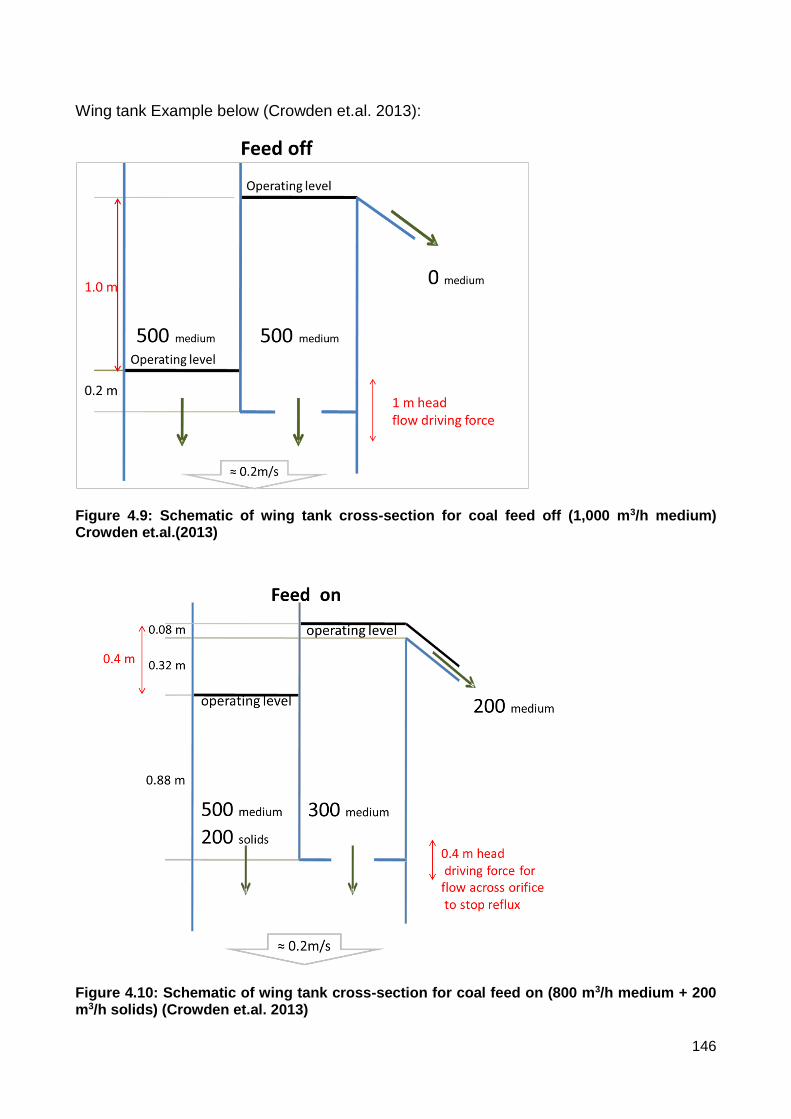
146

Wing tank Example below (Crowden et.al. 2013):

Figure 4.9: Schematic of wing tank cross-section for coal feed off (1,000 m3/h medium) Crowden et.al.(2013)

Figure 4.10: Schematic of wing tank cross-section for coal feed on (800 m3/h medium + 200 m3/h solids) (Crowden et.al. 2013)

147

The wing tank must meet two key objectives. Firstly, it must be capable of operating at a

constant level while receiving incoming feed solids and medium. Achieving a constant

level allows the DMC to be fed at a constant flowrate and pressure. In some plants this is

achieved by the use of a splitter box before the wing tank to separate excess medium off

into the correct medium sump (Crowden et.al. 2013). In other plants such as New Acland,

the excess medium is allowed to enter the seal side of the wing tank and then overflow at

the seal leg of the wing tank with the overflow feeding into the correct medium sump.

Variable speed pumps are also common in plants to balance out minor variances in wing

tank level to provide a more consistent feed to the DMC.

The key objective is to have a uniform downward flow rate to the DMC feed pump of

approximately 0.2 m/s. This reduces the tendency of more buoyant particles to raft inside

the wing tank, while being sufficiently low in velocity to avoid entraining air. (Crowden et.al.

2013) Maintaining a consistent downward flowrate means that coarse feed entering the

wing tank follows a direct path to the pump inlet. The profile of a wing tank is typically tall

and narrow to ensure a direct path to the pump and promote plug flow. Although flows

inside the wing tank are turbulent, it was noted by Askew (1983) that wing tank flows

resemble that of variable volume plug flow devices. This notion is supported by the RFID

residence time data collected in the New Acland plant. (as detailed in Chapters 3.3 and

3.4) Very little variation in travel times existed between the de-sliming screen and the

drain and rinse screens for particles following the same route as a piece of coal through

the wing tank and DMC.

The wing tank was modelled in a function outside of the main script called

wing_tankVec.m. The Wing tank function was a relationship between the feed to the wing

tank, the volumetric feed to the DMC and the volumes in the wing tank on the coal and

seal leg sides. Initially a boundary was assumed around the entire wing tank. Inputs to

the wing tank included initial volumes of the coal and seal sides of the tank, the coal and

medium flowrate into the wing tank from the desliming screen (to_wing) and the drained

medium returning from the drain side of the drain and rinse screens (from_DR_drain). The

drain was also multiplied by a splitter factor (y) which accounted for any proportion of

drained medium that was split to the coal side of the wing tank. In the New Acland case

study, y=1. The volumetric flow rate of the DMC feed pump at the base of the wing tank

was also considered (DMCfeedvol). Outputs of the wing_tankVec.m function included the

148

wing tank overflow (W_overflow) which flows from the seal leg to the correct medium

sump, the tank level and the seal level. (Figure 4.11)

Figure 4.11 Inputs and outputs to the Wing Tank function

The wing tank function calculated the levels in the wing tank and in the seal leg using a

spline equation which was based on the tank geometry (height to volume relationship) and

then used this to calculate the orifice flowrate and head in the wing tank. An orifice plate

which separated the coal side of the wing tank from the seal leg was considered in these

calculations due to its influence on relative head in the two sides of the tank. Under

normal operation, medium flows from the seal leg into the coalside of the wing tank to

deter rafting of coal into the overflow. The differential head between the coal-side and the

seal-side of the wing tank is significant in driving the flows through the orifice plate and

therefore determining the orifice velocity. The flow rate through an orifice is calculated as

follows (Crowden et.al. 2013):

Flow rate through an orifice

Q = C x a x SQRT( 2 x g x H)

Q Flow rate m3/s

H Head m

a Area of orifice opening in m2

g gravity constant 9.8 m/s2

C= 0.9 smooth, rounded, tube running fullC= 0.8 tube running fullC= 0.6 submerged square profile circular hole orificeC= 0.6 sharp lipped circular orifice

Example - orifice with C= 0.8, area 0.05m2 head H =1.0 m of fluid

Flow = Q = 0.8*0.05*SQRT(2*9.8*1)

Then convert Q in m3/s to m

3/h

Flow velocity through the wing tank orifice must be much greater than

0.2 m/s to avoid reflux.

21

149

For the New Acland CHPP dynamic model, the orifice calculation was modified to account

for flow direction through the orifice. To do this, a flow direction factor, k, was added and

this was influenced by whether the differential head (DeltaP) was positive or negative:

Qorifice = k* C * a * sqrt(2*g*abs(DeltaP)) 22

Where:

Qorifice – the flowrate through the orifice (m3/s)

dorifice = 0.310 metres (orifice hole diameter)

a = area of the orifice plate hole and is calculated as the area of a circle of

diameter, dorifice.

C = 0.6 for a submerged square profile circular hole (New Acland case)

g = 9.81 m/s2

DeltaP = is the differential head between the seal level and the coal-side tank

level

DeltaP = (seal_level) – (Wtank_level)

k = is the flow direction through the orifice plate. If the coal-side tank level is

higher than the seal seal-side level, Delta P is less than zero and therefore, k

will be -1. If flow is positive, ie. in the normal direction, k is +1.

As the square root of a negative number will result in an error, the absolute

value of Delta P was used in the orifice flow equation and the k value moved

outside of the square root part of the equation.

From the orifice flowrate, the velocity through the orifice can also be calculated as follows:

Vel_orifice (m/s) = Qorifice / a 23

Ideally the velocity through the orifice should exceed 0.2 m/s to prevent rafting. Under

normal operation, the seal level will typically be higher than the coal-side tank level.

During feed off conditions, that is, when no raw coal feed is present, the circulating

medium in the wing tank should be sufficient to maintain a seal level where medium is just

touching the overflow, ie. virtually zero overflow. (Crowden et.al. 2013) The coal-side tank

level is typically higher than the height of the orifice plate when running. The orifice plate

sizing is normally adjusted during commissioning to ensure that wing tank levels are

maintained during operation which in turn ensures a continuous head delivered to the

DMC pump. (Crowden, et.al. 2013)

150

Although the DMC feed pump is capable of variable speed operation, the pump speed at

New Acland is set as constant by the control room operator during normal running. Minor

adjustments may be made as the pump wears, and when grade changes require higher or

lower DMC pressures. The operator alters the pump speed until the desired pressure is

reached, and then leaves it unchanged until a new coal type comes through the plant.

When feed is added to the wing tank, there is sufficient free space designed into the coal-

side to accommodate the coal and medium. This additional coal increases the level of the

coal-side and therefore decreases the differential head between the seal side and coal

side. (Crowden, et.al. 2013) The correct medium and dilute pumps are also typically fixed

at constant speed. This means that the flowrate into and out of the wing tank changes by

the amount of returning medium and the amount of coarse feed entering the tank.

Once the orifice flowrate has been determined, the new seal volume (Sealvol) and wing

tank volume (Tankvol) could be determined by doing a mass balance around both sides of

the tank, considering the orifice to be one of the streams:

Sealvol= Sealvol_old + from_DR_drain .* y – Qorifice

This is the calculation of seal volume with zero overflow.

Tankvol = Tankvol_old + to_wing + (1-y)*from_DR_drain - DMCfeedvol +

Qorifice

A provision was made here for a plant where a splitter box exists above the wing tank to

divide the drain flows between the coal and seal sides of the wing tank, however, in the

New Acland case, one hundred percent of the flow was to the seal side (y=1).

The overflow from the seal side of the wing tank to the correct medium sump was then

determined using tank geometry to set limits. If the seal volume was below the volume of

the overflow, the W_overflow was set to zero cubic metres per second. If the seal volume

was greater or equal to the overflow volume, the following formula determined the overflow

rate:

W_overflow = (y .* from_DR_drain - Qorifice)

Once the overflow flowrate was determined, the new seal volume was able to be

calculated by considering the drainage flowrate from the drain and rinse screens, the flow

through the orifice and the wing tank overflow.

151

Sealvol= Sealvol_old + y*from_DR_drain - Qorifice - W_overflow

The wing tank function outputs return the values of seal level, wing tank level and overflow

volumetric flowrate back to the main script. The medium to coal ratio is then calculated in

the main script and also the DMC pressure based on the head from the wing tank.

A clean_coal function is used to partition the raw coal based on its washability for an

initially pre-determined value for d50c (cutpoint) and Ep. Here, the Whiten Partition model

has been used. The washability data uploads from a .csv file. This format was chosen to

enable multiple washability data sets to be used. The Ep and d50c values will change and

update as the model iterates through the set number of iterations. It should be noted that

Ep values determined by plant experiment or tracer test may differ from the Ep values in

the empirical model. This is a common issue when relating the JKMRC Wood model back

to plant data and is often the reason for an adjusted Ep. The clean coal function outputs

the mass of partitioned clean coal, volume of clean coal and clean coal density back into

the main script. The volume pumped from the wing tank (DMCfeedvol) then considers the

clean coal density to calculate mass flowrates from the partition model.

As the coal circulates through the dense medium circuit, some breakdown of clays and

small coal occurs. This is accounted for using a slimes factor. The size consistency of the

slimes is predetermined using a slimes factor multiplied by the size distribution of the raw

coal feed. An assumption has been made in the model that 2% of the raw coal breaks

down and becomes an integral component of the medium. The new size distribution is

adjusted according to the slimes factor in each iteration. This is important for the model as

in practice, a build-up of contamination, or non-magnetics will occur, particularly if the

bleed to the dilute is closed. This level of non-magnetics changes and affects the stability

of the medium. As the vectors in the model are component vectors split by coal, water,

magnetics and non-magnetics, it is possible to change the components using the slimes

factor calculation.

Drain and Rinse Screens

The drain and rinse screens are modelled based on Firth and O’Brien’s medium recovery

models Crowden et.al (2013). These models calculate the medium drain rates and fines

recovery for the screens using the flowrates calculated and product by size data adjusted

for slimes breakdown. Information about screen apertures, open area and screen

152

dimensions are required for this part of the model. The calculation of the amount of water

reporting to the oversize flow stream, Rf and the number of presentations of the particles

to the screen deck surface is determined. The effect of the N value is to influence the

curvature of the partition curve. As a screen wears, the amount of undersize reporting to

the drain will increase. The percentage of material reporting to the drain (drain_percent) is

then used in the main script. This is calculated for all drain screens, product and reject,

and enables determination of the drained medium returning to the wing tank.

Drain = Pdrain +Rdrain

from_DR = Comb_Drain_delay (Drain,Drain_delta)

The latter relationship is a function that uses the delays calculated from residence time

testing to determine the stream from the drain and rinse back to the wing tank seal leg.

The remaining medium not reporting to the drain side is accounted for by difference and is

sent to the rinse side of the drain and rinse screens. A similar calculation is used for the

rinse screen model, however the amount of rinse water added is also taken into account.

The function “Rinsepd2” performs the calculation of partition of the rinse section of the

drain and rinse screen and then returns the values for the product rinse volume, the

amount of water and rinse water to the dilute back to the main script. The size distribution

is then used to partition solids on the rinse screen. The proportion of rinsed medium to the

dilute is then calculated for each screen. The clean coal and reject leaving the end of the

rinse screens is then determined, accounting for some adhesion losses of magnetite on

the coarse material entering the launders.

The final calculation sums the rinse medium flowing to the dilute as follows:

Rinse_to_dil = PRDilute + RRDilute

where PRDilute is calculated using the RinsePD2 function and RRDilute is

calculated using the RRinse function and both represent the rinsed medium flows from the

drain and rinse screens to the dilute sump. Once again, a delay is added

(Comb_Rinse_delay) to account for time taken for flows to reach the dilute sump. The

reject coarse entering the coarse launder is also accounted for by difference with adhesion

losses taken into account.

153

Correct Medium Sump Balance

Once drain and rinse flows have been calculated, the correct medium sump balance can

be done. The geometry of the correct medium sump is a conical bottomed vessel with a

total volume of 35 cubic metres. The incremental changes in volume with respect to

height have been calculated based on the tank geometry and with the use of the Matlab

spline function on the conical section, the tank level can be determined from tank volume.

For the cylindrical section, a regression equation was determined to accurately predict the

height per unit volume. Once the slurry level in the sump reaches the bottom of the

overflow, the program calculates the volume of excess slurry as the overflow amount after

accounting for inputs and outputs to the tank.

To account for dynamic changes with time, the old volume (Sump_vol = CMvol_old) is

recorded from the previous value and this is then added to by applying the volume balance

around the sump for the next increment. The function for this calculation is

CorrectSumpVec. In order to complete this calculation an initial value of flow from the

magnetic separator is assumed. Similarly, the pumping rate from the Magnetite Pit

(from_Mpit) is also assumed. The calculated volume is then recorded as the new value for

Sumpvol and the next iteration commences. The level in the correct medium sump from

the spline equation is then used to calculate the pump head for the correct medium pump.

The Correct sump volume is then updated as follows:

Sump = CMVol_old + from_MagSeps + W_overflow + from_Mpit

CM_Vol = CMVol_old + from_MagSeps + W_overflow + from_Mpit – from_CM

where from_CM is the proportion of the sump pumped out in m3/s

and W_overflow is the overflow from the wing tank

The overflow of the correct medium sump is calculated only if the level exceeds the height

of the overflow pipe. This is calculated as the difference in the volume (CM_vol) and the

pumpout volume (from_CM).

The pipework exiting the correct medium sump has an automatic water addition valve

before the pump and then the line splits after the pump into a bleed stream into the dilute

sump, and a feed stream to the desliming screen. The function of this auto water valve

154

(control_water) has been described earlier and the water stream (control_water) combines

with the water pumped from the correct medium sump (from_CM) to create a larger stream

This variable is still called “from_CM” but as it is later in the code, the variable updates with

the new figure.

Due to the location of the 100mm diameter bleed line on the top of the horizontal 600mm

diameter correct medium pipe (Figure 4.12), it is theoretically possible that some settling in

the pipe may result in lower density material preferentially entering the bleed line, however

this cannot be determined without further sampling.

100mm

diameter

0.3m

1.5m

3.6m

elevation

from

pump

outlet

on

ground

floor

Three elbows between

pump and bleed line

Butterfly Bleed Valve

Correct Medium Line

330mm diameter

Nucleonic Gauge

Figure 4.12 Elevation sketch of the 100mm bleed line tee off the main correct medium line.

Occasional blockages due to rafting coal suggest that the flowrate through the wing tank

orifice is not always sufficient. For the purposes of the model, the same composition is

assumed for the correct medium line and the bleed tee off point. This is important to note

because the nucleonic gauge is situated downstream and is also in a horizontal section of

pipe. Calculation of the bleed stream to the dilute sump is achieved using a manual input

155

variable which splits the correct medium stream by a set proportion. The bleed to dilute

line (Bleed_to_Dil) is calculated to include a delay for transport time. The dilute sump

balance is then able to be determined.

The Dilute Sump

The dilute sump is a cylindrical vessel with a conical bottom and a total volume of nine

cubic metres. The geometry of the sump was determined from the construction drawings

and was used to calculate the volume in a similar manner to the correct medium sump

calculation. A spline equation was then used to determine sump level for a specific

calculated volume. This spline calculation is part of the DiluteSumpVec function which

uses inputs of return rinse medium (Rinse_to_dil), make-up water (Clarif_water), and floor

sump contents (Floor_drain). An initial volume (DilVol_old) is set and this value is

replaced with each new iteration. Since the floor sump pumps its material onto the end of

the rejects screen and into the underpan, which flows back to the dilute sump, it was

assumed that the floor sump pumps directly into the dilute sump for the purpose of the

model. Further, it was noted that in an overflow situation, both the dilute and the correct

medium sumps would flow into the floor sump and then back into the dilute sump and

therefore, the floor sump could be considered as part of the dilute sump system for the

purpose of modelling the dilute sump balance.

The dilute sump function outputs are tank level (Diltank_level), dilute sump overflow

volume (Dil_overflow), new sump volume (Dil_Vol), and the pumpout rate to the magnetic

separators taking into account any transport delays (from_Dil). Since magnetic separators

typically do not cope well with surges in flow or inconsistent levels, the pump would

normally be run at a fixed speed to ensure consistent flow.

Magnetic Separators

The magnetic separator section of the model is calculated in a separate function,

MagSepVec2 which is based on Firth and O’Brien’s work in Crowden et al. (2013). A

magnetic separator concentrate and tailings stream have been determined from this

function. These streams return to the correct medium sump and to the desliming water

make-up sump respectively. The proportion of magnetite losses and removal of non-

magnetics can be calculated also using this function. Some difficulties were experienced

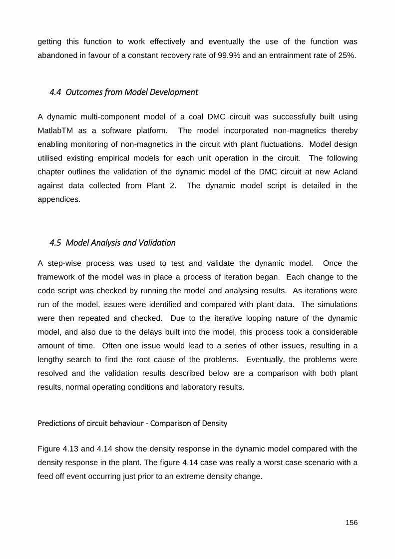
156

getting this function to work effectively and eventually the use of the function was

abandoned in favour of a constant recovery rate of 99.9% and an entrainment rate of 25%.

4.4 Outcomes from Model Development

A dynamic multi-component model of a coal DMC circuit was successfully built using

MatlabTM as a software platform. The model incorporated non-magnetics thereby

enabling monitoring of non-magnetics in the circuit with plant fluctuations. Model design

utilised existing empirical models for each unit operation in the circuit. The following

chapter outlines the validation of the dynamic model of the DMC circuit at new Acland

against data collected from Plant 2. The dynamic model script is detailed in the

appendices.

4.5 Model Analysis and Validation

A step-wise process was used to test and validate the dynamic model. Once the

framework of the model was in place a process of iteration began. Each change to the

code script was checked by running the model and analysing results. As iterations were

run of the model, issues were identified and compared with plant data. The simulations

were then repeated and checked. Due to the iterative looping nature of the dynamic

model, and also due to the delays built into the model, this process took a considerable

amount of time. Often one issue would lead to a series of other issues, resulting in a

lengthy search to find the root cause of the problems. Eventually, the problems were

resolved and the validation results described below are a comparison with both plant

results, normal operating conditions and laboratory results.

Predictions of circuit behaviour - Comparison of Density

Figure 4.13 and 4.14 show the density response in the dynamic model compared with the

density response in the plant. The figure 4.14 case was really a worst case scenario with a

feed off event occurring just prior to an extreme density change.

157

0 100 200 300 400 500 600 7001.2

1.4

1.6

1.8

2

Wood Model Onstream Densities

Time, s

RD

DMC Underflow Density

DMC Overflow Density

Nucleonic Density

Density Set Point

0 100 200 300 400 500 600 700

0.6

0.65

0.7

0.75Onstream Density Differential

Time, s

Diffe

ren

tial

Differential

Figure 4.13 Matlab density (minutes 1=60s, 2=120s, 3=180s, 4=240s, 5=300s, 6=360s, 7=420s). Plant feed variation was switched off in this particular instance.

Figure 4.14: Plant data from 25/3/2014 showing plant response to an upwards stepwise density set point change.

19 mins

3 mins

158

Figure 4.15: Dynamic model density response was too fast.

The density controller gain was adjusted until it resembled the plant in figure 4.14

Figure 4.16 Dynamic Model Density response was adjusted to give a more realistic time for density change.

5 mins

159

Figure 4.17: Plant start up condition at time zero with a density set point rise at 5000s and dynamic model response compared against set point.

Figure 4.17 above shows the densities of the medium and set points from an initial start up

condition. At start-up, delays are significant in influencing flows to various parts of the

circuit. This also influences the action of the automatic water valve density adjustment.

Modelling of faster methods to achieve stable density operation after start-up (eg. an

overdense sump) would be a useful future application of the dynamic model.

Figure 4.18 shows another density response to a drop in density. In this situation the

density response is faster, dropping from 19 minutes to 5 minutes. By comparison, the

dynamic model appears to respond relatively well, albeit a little slower than the plant

situation (Figure 4.19a) however this is somewhat dependent on the gap that the density

needs to move. Opening the bleed while changing density resulted in a longer time than

when the bleed was closed. This is discussed further in the discussion around Fig 4.24

The speed of density movement can be adjusted to match plant outputs using the

autowater controller. Fig 4.19b shows a different density change and the response was

faster at the higher density range.

160

Figure 4.18: Plant data from 26/03/2014 showing plant response to a downwards density set point change

Figure 4.19a Dynamic model was adjusted to drop the density in the plant from 1.35 to 1.30

5 mins

11 min

161

Figure 4.19b Dynamic model was adjusted for a different density drop in the plant. Here, the response of the controller is faster, partly due to the higher operating density range.

4.3 mins

162

Predictions of circuit behaviour - Comparison of DMC Pressure

In addition to the density parameter, the model also considered the DMC pressure. This is

usually in the form of a gauge located in the feed line to the DMC, and often within one

metre of the DMC unit. The figures 4.20 to 4.22 below show the plant results compared

with the dynamic model result for pressure. On the 25th March the plant feed was turned

off on two occasions, the latter occasion being for a prolonged period of time. The causes

of the feed off periods in this case were unrelated to the dense medium circuit. One of the

conveyors had to be shut down due to a tracking issue which took some time to rectify. As

a result of the lengthy outage, density (Fig 3.8) and non-magnetics concentration (Fig 3.9)

initially dropped considerably. Upon re-starting from the feed off condition, it took time for

the density to build up and for non-magnetics to re-establish in the system. Had the

control room operator reduced the amount of water flowing off the desliming screen into

the wing tank, the density could have been maintained at a higher level, thereby reducing

the amount of time for density to recover. Similarly, the bleed could have been closed to

reduce loss of non-magnetics while the plant feed was offline. Note the pressure response

to the short plant feed outage (t = 20minutes, Fig 4.20) was considerably more rapid than

the response for the longer feed outage (t = 180 minutes, Fig 4.20).

Figure 4.20: Typical pressure response (red) during plant events. Two feed off periods occurred during this particular test work. (25/3/2014) The causes of the feed off periods in this case were unrelated to the dense medium circuit. One of the conveyors had to be shut down due to a tracking issue which took some time to rectify.

163

Figure 4.21: Pressure curve from the dynamic model. The curve is similar to the plant start up after the feed off events in the previous graph (at 180 mins Fig 4.20).

Figure 4.22: Another example of DMC pressure modelled from plant start-up. In this case, the time scale is longer. Note: pressure change at 5000s (83mins) was due to a density set point change upward in the model.

Predictions of circuit behaviour - Comparison of Non-magnetics

The level of non-magnetics in the correct medium was expected to change over time, both

with removal of non-magnetics by bleeding out of the correct medium into the dilute, and

also through breakdown of clays in the raw coal feed. This was simulated using a slime

factor (essentially an allowance for breakage) in the dynamic model. Plant data collected

and analysed for percent non-magnetics aligns with the dynamic model responses. Figure

164

4.23 below shows a comparison of % non-magnetic material in the correct medium after a

plant start up over time (4.23a) with the plant model dynamic response (4.23b). (Firth

et.al. 2014).

Figure 4.23a: Build-up of % non-magnetics from plant start up condition (Firth et.al 2014). (Timescale conversions: 20 mins = 1200 seconds, 4500s = 75minutes)

Figure 4.23b: Build-up of non-magnetics in the dynamic model from start-up. (Density change at 5000s, bleed opened at 4400s)

While the dynamic model response is slightly faster, this can vary with the amount of bleed and the

relative amounts of non-magnetics at the start. The model reaction to opening the bleed is shown

in Figure 4.24 a and b. If an operator opens the bleed, non-magnetics can be lost as rapidly as it is

generated through breakage, or, as was demonstrated in the plant experiments, non-magnetics

165

could be lost at a faster rate than it was generated. Figure 4.24c shows the effect on the dynamic

model of also adding magnetite with the bleed open. (with the same conditions as in 4.24a and b.)

Figure 4.24a: Bleed opened fully at 5000 seconds. 4.24c is the response from the model.

Figure 4.24b: Model response to bleed being opened fully at 5000 seconds. Note the drop off in the amount of non-magnetics in the circuit.

166

Figure 4.24c: Model response to bleed being opened fully at 5000 seconds with magnetite addition at 6500 seconds. Note the additional drop off in the amount of non-magnetics in the circuit once magnetite is added. This is in line with expectations.

Predictions of circuit behaviour - Comparison of Plant Results

In order to compare typical plant operating parameters, the plant process flow drawings

(PFD’s) were analysed. It was noted that the plant typically operates at 500 to 550 tonnes

per hour of raw coal feed unless there is a problem which requires the plant to operate at a

lower rate, for example, a constrained thickener. Much of the experimental data collected

was at the 550 tph operating rates, however, the PFDs indicated that the plant name-plate

capacity was lower. Despite this difference in tonnage, it was felt that the PFDs gave a

reasonable estimate of flowrate ratios through the plant for the purpose of designing the

dynamic model.

The wing tank level and seal level can be seen in the first graph of Figure 4.25. It would

normally be expected that the seal level would exceed the height of the wing (coal) side in

the wing tank and this is demonstrated in the graph. It is also clear that the seal in the

tank has reached its normal overflow condition (Figure 4.26).

Figure 4.25: Wing Tank and seal leg levels. Seal level is in overflow condition.

167

Figure 4.26: Wing tank overflow from the seal leg into the correct medium sump. After the initial flows at start-up, flow steadies.

Figure 4.27: The drain and rinse underpans drain back to the correct medium sump. There is an initial delay until feed comes on. Flow then steadies.

The flows of drain-side medium returning from the drain and rinse screen to the seal leg of

the wing tank are visible in figure 4.27 above. There is some initial instability, but flows

quickly smooth out.

168

Figure 4.28: Coal and medium flows from the desliming screen to the wing tank. At startup there is an initial surge. It is thought that this surge relates to a slight mis-match in delay times in the model.

Figure 4.28 shows the coal and medium flows from the desliming screen to the wing tank.

Although on normal plant startup there may be an initial surge, it is not expected to be of

this magnitude. It is thought that fluctuations in the automatic water addition and a mis-

match in delays are responsible for the apparent surge of medium on the graph. Delays

were measured between the desliming screen and the drain and rinse screens and

between the correct medium sump entry point and the drain and rinse screens, however

some interpolation of the results was necessary to determine the delay times for smaller

sections of the circuit. The accuracy of the delays could therefore be considered to be

less precise for the sections around the wing tank. The coal and medium from the deslime

graph in Fig 4.28 can be seen to reflect the wing tank overflow in figure 4.26. It can be

seen that the majority of the surge carries over into the seal leg and overflows the wing

tank. The seal leg essentially has a smoothing effect on the circuit and by the time the

coal and medium arrives at the DMC, the flows have smoothed out considerably. Figure

4.29 and Figure 4.30.

Figure 4.29: Coal and medium flows to the DMC

169

Figure 4.30 Flowrates into and out of the DMC

Flowrates into the DMC were smooth despite a surge in medium coming from the desliming screen into the wing tank. This graph also shows the DMC underflow and DMC overflow flowrates of medium and coal travelling to the drain and rinse screens. The surge is smoothed out using the seal leg overflow on the wing tank.

The level in the correct medium sump is also fairly steady (Figure 4.31) and the surge

assists in filling the correct medium sump.

Figure 4.31 – The level in the correct medium sump helps to absorb the surge coming from the wing tank seal leg.

During start up, the medium to coal ratio is initially unstable but steadies to hover around

4:1 which is within the normal range for good operation. (Figure 4.32)

170

Figure 4.32: The medium to coal ratio is approximately 4:1 which is within expected range.

Figure 4.33: Plant flowrates for Correct medium and magnetite.

The initial surge in correct medium pumped from the correct medium sump (Fig 4.33) is

related to the automatic water addition valve on the base of the sump.

Figure 4.34: Flows from magnetic separator concentrate stream back to the correct medium sump.

171

The graphs in Figure 4.33 and 4.34 above can be seen to reflect the correct medium

flowrate and additions of concentrated magnetite from the magnetic separators. During

the test run, magnetite from the magnetite pit was also added to the circuit in Figure 4.35

below. This was used to stabilise upward density adjustments.

Figure 4.35: Fresh magnetite addition from the magnetite pit

This magnetite addition occurred at start up and just prior to the upward density change at 5000 seconds. This was found to assist with shortening the time of the density adjustment. In practice, this is done regularly by operators prior to upward density set point changes.

To assist with density control, a water addition control valve exists at the base of the

correct medium sump and is controlled using a feedback control system based on the

density set point. When the density is detected as too high, the water valve is opened to

compensate by adding water to the system. The function of the auto water valve is shown

in the figure 4.36 below. It is clear that in the initial start-up, this water valve causes the

surge in the medium flows (Figure 4.33). Introduction of an increased delay or better

tuning of the proportional integral controller may help to alleviate this initial plant surge.

Figure 4.36 Automatic water addition valve for density adjustment

172

The automatic water valve on the base of the correct medium sump is controlled using a feedback loop to the nucleonic gauge. There is considerable instability initially which leads to a surge in medium at start-up.

Predictions of circuit behaviour - Dilute circuit operation

Dilute sump operation is demonstrated by the figures 4.37 to 4.41 below. Rinse water

from the drain and rinse screens flows back to the dilute sump and flows are generally

steady. The bleed to the dilute was set as a constant value after a short delay. The

operators in the plant normally operate this valve to moderate volume.

Figure 4.37 Flow from the rinse underpan of the drain and rinse screen to the dilute sump.

Figure 4.38 Bleed to the dilute has been set as a fixed value with a small delay.

173

Figure 4.39 Flow rate of clarified water make-up into the dilute sump to maintain level. In practice some centrifuge effluent would also be present.

Figure 4.40: The level in the dilute sump from start – up condition.

Figure 4.41: The magnetic separator is fed from the dilute sump. This pump is set to deliver based on the head in the dilute sump.

174

Predictions of circuit behaviour - Comparison of the Component Balance

The component balance for each unit operation was checked to ensure that all streams in

and out and all components were consistent. This was done on a unit by unit basis as the

model was developed. Any discrepancies in the balances were corrected as the model

was built. The differential was a measure of circuit stability and can be seen in figure 4.42

below. It relates directly to the proportion of non-magnetics in the medium. Initially the

differential is higher but as the level of non-magnetics climbs, the differential drops. Figure

4.43 and 4.44 have been added to indicate the corresponding differential changes with

changing density set point. As is evident from the graphs below, the differential remained

within in the stable region below 0.5, though was relatively high.

175

Figure 4.42 The differential is a measure of the difference between overflow and underflow density. The drop in differential can be seen also in the non-magnetics graph below and corresponds to the density change at 5000s.

Figure 4.43 Corresponding non-magnetics concentration

Figure 4.44: Corresponding change in density setpoint. Figs 4.42 and 4.43 show the change in non-magnetics and differential for comparison.

176

4.6 Model Validation Conclusions

The dynamic model developed has demonstrated the ability to realistically predict typical

plant behaviour. Sump levels, DMC pump pressures, density changes and flowrates have

been successfully replicated, as has the build-up of non-magnetics in the medium. Sump

levels were shown to fluctuate and the medium to coal ratio controlled within a reasonable

range. The verification of the dynamic model has shown that the model generally

describes circuit behaviour and that the model will be able to be used for prediction of

behaviour as well as for operator training. Residence times for particles from the RFID

tracer work were used to predict delays in the model.

As the structure of the dynamic model is still in its rudimentary form, the opportunity exists

to take this modelling work further. The addition of more user friendly features such as a

graphical user interface would be helpful as would the opportunity to incorporate or

substitute in different unit operations. Future refinements would benefit from using this

model to analyse a range of different coal washabilities. As most coal producers are

familiar with Excel but not with Matlab, the option of an excel spreadsheet seems

reasonable as a future addition.

177

5 Conclusions, Applications and Further Work

5.1 Conclusions

For convenience, the conclusions have been drawn in the order of appearance in this

thesis.

It was identified through an extensive literature review that:

Past research into dynamic models has been limited by a lack of available plant

data, computer memory and processing capability. Empirical models for DMC

circuits such as those detailed in Crowden et al. (2013) have been significantly

improved since early modelling work was done and a wider range of plant

information is now able to be collected.

Dynamic modelling of changes in the coal medium composition has not been

sufficiently studied. Recent studies of changes in DMC medium composition

(O’Brien, et al. 2013) have shown that the level of non-magnetics influences

medium stability when targeting a low density cut-point and therefore has an

influence on plant behaviour.

Novel instruments in use at the New Acland CHPP provided information that was

previously unavailable.

Advancements in RFID density tracer technology created an opportunity for

additional plant data such as residence times for individual density tracer particles

to be collected using a novel method.

To address the research deficiencies identified, a programme of experimental work was

devised and a dynamic model was developed. Plant observations and physical

measurements were conducted as part of the experimental work phase of the research

and were later used to verify the model. Findings as a result of this experimental work are

detailed below:

178

Plant work involved the testing of a number of cases. The findings of each case are listed

below:

Case A: Good density change

o After a density increase during stable operation, the level of non-magnetics

was found to reduce with an increase in correct medium bled to the dilute

circuit.

o A feed off event which occurred during the trial demonstrated a rapid loss of

non-magnetics from the medium, suggesting that the amount of non-

magnetics in the coarse coal circuit is strongly affected by the feed.

o Despite a low differential (stable medium) and a carefully orchestrated good

density change, the medium took over an hour to recover back to the level of

non-magnetics before the density change.

Case B: Unstable Volume

o When operating at a high level in the correct medium sump, and at a low

density set point, the plant demonstrated difficulty in maintaining a sufficiently

low density due to excess magnetite. This suggested that an alternative

means of removing concentrated magnetite such as an over-dense or

magnetite pit return line was needed as an alternative to returning magnetite

to the correct medium sump.

o When the correct medium sump and the dilute sump were in an overflow

situation, the level of non-magnetics also became difficult to control. An

initial drop in non-magnetics was noticed upon opening of the bleed to 100%,

and a slight recovery of non-magnetics was noted when the bleed was

closed down to 20%.

o In a situation of unstable volume, it is difficult for the plant operator to

achieve stable density operation. Volume control becomes a predominant

issue at the expense of non-magnetics and density control.

Case C: Stepwise density change

o A step-wise density change resulted in a slower density response when

compared with a single change in density.

179

o The level of non-magnetics dropped markedly when the feed was left off for

an extended period of time. Density also dropped.

o The level of non-magnetics dropped when the bleed was opened, and began

rising when the bleed was closed.

o After start up, the level of non-magnetics took over 60 minutes to return to

prior levels despite operating on a high relative density.

o Time taken to reach density was slower when the amount of non-magnetics

was low and the plant feed had been off for a considerable time. Yield

losses were estimated at 17% over 11 minutes.

Case D: Low density stability

o Non-magnetics levels did not respond as well when sumps were in an

overflow situation, however a drop in non-magnetics was noticeable when

the bleed was opened.

o Stability at low density was impacted by volume control due to excess

magnetite.

o Due to the fact that the plant had run at very high density just prior to the low

density change, the medium was very stable on the test date and no surging

events occurred.

Case E: Desliming sprays response test

o Closing the desliming sprays had the effect of rapidly increasing the level of

non-magnetics in the medium.

o The rate of build-up of non-magnetics was 2% over 2 minutes.

o The use of desliming sprays to control non-magnetics was not feasible for

this particular plant design due to the sensitivity of the water balance,

however the concept may work for other designs.

o Ultimately another means of adding non-magnetics to the medium such as

thickener underflow may need to be investigated.

Case F: Tracer Testing

180

o Recently developed RFID density tracers were used to measure the

residence times of individual particles travelling through the DMC circuit.

This novel method of measuring residence time had not been previously

done.

o RFID residence time testing of coal particles travelling through the dense

medium yielded valuable information on time delays within the circuit and

assisted with model development.

o Times measured for tracers to travel through the DMC circuit were

surprisingly short, with the times from the desliming screen through the DMC

to the drain and rinse screens ranging from thirty-six seconds to just over two

minutes. This route was representative of large coal particles travelling

through the circuit. There was no significant difference based on the density

of the coal particle for this pathway.

o The time for a coal particle to travel from the weightometer to the drain and

rinse screens ranged between two minutes and three and a half minutes.

This highlighted the rapid response of the circuit to changes in feed.

o The time taken for particles to travel through the medium differed for denser

tracers of the same size when compared with low-density particles and with

particles of near gravity. This was concluded to be the result of settling out

of heavier particles from the medium, and floating of lighter particles out of

the medium. Particles that were close to the cut point had a strong tendency

to flow as part of the medium and not segregate out. This resulted in shorter

time travel for near gravity particles. Particles of very high and very low

density took up to 39 minutes to travel through the circuit.

o The prediction of cut point for different sized tracer particles showed an

unusual cut point reversal between the 13mm RFID and 32mm standard

tracers. This was observed on three separate occasions and it was

concluded that the effect was real. The observations were also confirmed

when a literature review of a thesis by Wood (1990) demonstrated similar

effects. It was also determined that the original cause postulated by Wood

was incorrect as no float sink chemicals were present in the case of the

181

tracer tests at New Acland, therefore eliminating chemical absorption as a

possible cause.

The outcomes of the experimental work were used to develop and verify a dynamic model

of the New Acland dense medium circuit. The model used existing empirical relationships

that are accepted by industry as providing reasonable predictions of plant behaviour. Non-

magnetics concentration in the medium was predicted using a breakage model and results

were verified against past plant event data collected during the experimental work stage.

The development of a dynamic model of a coal dense medium circuit was facilitated by the

use of novel plant instrumentation at New Acland, advances in RFID technology, the

collection of a broad range of data from plant events, and an in-depth investigation by

CSIRO into medium behaviour. The findings from the modelling work are detailed below:

The construction of a multi-component dynamic model of a coal DMC circuit was

successfully achieved and a breakage model was incorporated into the dynamic

model enabling monitoring of non-magnetics in the circuit.

The dynamic model was able to achieve realistic predictions of plant behaviour.

This was demonstrated using the examples of density, non-magnetics and DMC

pressure. Sump levels were shown to fluctuate and the medium to coal ratio

controlled within a reasonable range.

The model was tested on a limited range of washability data, however could be

expanded to other washability data sets in future.

The verification of the dynamic model has shown that the model generally describes

circuit behaviour and that the model will be able to be used for prediction of circuit

behaviour as well as for operator training.

This research differs from past research efforts in that novel instrumentation and

techniques have been used to collect experimental data, and the inclusion of medium

components to predict the proportion of non-magnetics in the medium has not previously

been attempted. Changes that result from fluctuations in magnetite additions, density

adjustments and the bleed valve which diverts non-magnetics to the magnetic separators

can also be incorporated into the dynamic model. Benefits derived from this project

182

include improvements to plant operation through better use of dense medium circuits and

improved understanding of dense medium circuit fluctuations. Potential applications of this

model and future research areas are identified in the following chapters.

183

5.2 Applications of the Dynamic Model

The research undertaken as part of this PhD was done with a goal of generating a net

improvement for coal CHPPs. Improvements in yield and combustible recovery are

always sought after and this has been kept in mind in the design of experiments. Fast

density changes can reduce yield loss from misplaced coal, however as the time period of

yield loss is small during a density change, losses may not be noticeable unless data on

coarse product and reject mass flowrates is recovered in real time from instruments. Non-

magnetics is unseen in the dense medium, and operators cannot easily control it without

knowing what drives it. A plant operator can observe DMC surging event by visually

monitoring the rejects screen loadings and product weightometers, but may not realise that

the cause of the surging may relate to unstable medium or a lack of non-magnetics. If a

surge is observed in real time, changes can be made to the level of non-magnetics to

better stabilize the medium. Clearly, there are opportunities to recover coal that are being

lost due to either a lack of instrumentation, or a lack of knowledge of what is happening in

real time.

The dynamic model can help to identify opportunities to recover coal by simulating real

plant events and allowing the operator or plant metallurgist to see what happens to various

outputs in response. The applications of this model as a tool are for education purposes,

but also for control system and plant improvement. Designers can use a dynamic model

to try different design improvements or plant layouts. In Australia, we are fortunate that

many dense medium plants across the country are fairly similar in design. Some may

have slightly different circulation routes of the medium, but essentially there are similarities

that can lead to a more routine application of the research across the industry. The plant

at New Acland was a single stage DMC and spirals circuit, with the absence of flotation.

Some plants that process hard coking coals, such as those in the Bowen Basin, have

multiple stages, and flotation. In future, it would be beneficial to apply the model to a more

complex plant and include the finer circuits.

Dense medium circuits have evolved over the years from falling density systems with over-

dense sumps and magnetite thickening circuits, to the present day rising density systems

with faster response and considerably fewer items of larger capacity equipment. Certainly

there has been a saving in terms of capital with these newer designs, but the metallurgical

184

cost of this change has not been entirely clear. The observations made at New Acland

CHPP suggest that at very low operating density set points, the plant experienced

difficulties in removing magnetite from the circuit. This led to an overflow situation in the

correct medium and dilute circuits where excess water was added by the automatic water

valve to compensate for the concentrated magnetite being added back into the correct

medium by the magnetic separators. This was a case of a rising density system working

against itself. The operators’ normal solution to the problem was to plan in advance for a

density drop by removing any build-up of excess magnetite from floor sumps and to lower

sump levels in the hours prior to the downward density change. In the case observed, an

extreme density change from 1.6 to 1.35 was noted. This change proved too much for the

system to cope with, and the resulting overflowing of sumps to the CHPP floor

demonstrated the relative merits of over-dense storage for returning concentrated

magnetite. Trialling the return of over-dense magnetite to the magnetite pit or into an

additional over-dense sump could be done using the dynamic model before any capital is

spent on equipment.

Given that magnetic separators are now far more efficient leading to the virtual elimination

of auxiliary magnetic separators from circuits, the amount of equipment required to support

an overdense system in a modern rising density plant is likely to be far less than for a

falling density plant. Magnetite thickeners have been largely eradicated in favour of

cyclone thickeners, or direct feed of magnetic separator concentrate into the correct

medium stream. Diverting the magnetic separator concentrate stream to the magnetite pit

may be the simplest solution, allowing the operator to hold back some magnetite when

orchestrating a density change downwards, or to quickly add concentrated magnetite to

rapidly bring the density up. In some cases, the solution may lie in a splitter arrangement

where plants can divert excess magnetite back into the magnetite pit when targeting a low

density. The most economical method of trialling the change would be to assess

performance using the dynamic model. If the dynamic model was able to demonstrate that

the change would be of benefit, then plant design for either a pilot or full scale trial could

commence.

A key benefit that should be seen from dynamically modelling an over-dense system would

be the relative reduction in the time required to achieve the target density. It has been

established from the experimental data, that a single density change rather than an

incremental change reduces the time taken to reach a target density. Where a density

185

change up occurs, capacity to add extra concentrated magnetite via an over-dense system

would suggest that the density response could be achieved faster, thereby losing minimal

yield during the adjustment period.

A cheap interim solution to achieving rapid density change might include installation of an

air-sparge in the base of the correct medium sump to assist with better mixing of the

medium in the sump. This again could be tested using RFID tracers and modelling the

change in delay times.

The control of non-magnetics during a density change was found to be achieved by turning

off the de-sliming sprays. Before implementing an engineering change to add dense

medium non-magnetics in metered amounts, the build-up of non-magnetics could be

simulated in the dynamic model. Research work by CSIRO is currently underway to add

non-magnetics back into a dense medium circuit and the outcomes of this work could feed

into dynamic modelling.

The use of RFID tracers to measure partition performance of the coal was a great

advancement on existing tracer technology. Whereas a small army of seven or more

volunteers were required to run a standard tracer test, the RFID tracers were able to be

achieved using one to two experienced people. Recent work at other sites has led to

development of permanent antennae designs which enable the plant metallurgist to run

regular checks on their coal types. This is a remarkable change from the industry status

quo. Novel application of the RFID tracers for residence time measurement could also be

applied to a much broader context. The RFID technology could be used to track coal

quality by following batches from specific strip, block and seam locations in the mine

deposit through to the port. This would enable ports to keep track of coal types and their

origins by means of mounting antennas over conveyors. Similar uses could be applied to

the rail lines where batches or individual rail wagons could be tracked and then modelled

in a dynamic model.

Dynamic modelling and RFID technology could be further used to link with geological

modelling to provide the CHPP with instant feed washability information. Identification of

bottlenecks and lead times in the supply chain could be accurately determined using RFID

technology to assist with observations.

186

5.3 Recommendations for Further Work

The development of a dynamic model of a dense medium cyclone circuit has led to many

opportunities for further work. This research modelled a single DMC circuit for a thermal

coal operation. Scope exists to expand the modelling work into other plants with

secondary DMC’s and also plants that operate within other density ranges. The dynamic

model could be refined with the inclusion of other unit operations and a graphical user

interface. Further testing at other sites would assist in tuning the model.

Other enhancements could include the addition of an over-dense system and use of the

model integrate bore core washability data for a particular mine. Long term use of Matlab

may be difficult due to its high cost to industry participants, and it may be better to adapt

the model into other software options such as a macro operated Microsoft Excel product,

or a C++ program in future.

The level of non-magnetics measured during plant experiments as part of this and other

ACARP projects suggests that it would be very useful to have an online non-magnetics

gauge in place. Similarly, the under-pan density gauges have proven sufficiently robust to

be installed in other plants and to be used for measurement of differential and therefore

medium stability. The installation of a computer console in the plant control room which

reads tags from the plant instruments could allow the operator to look at online washability

using the dynamic model and to identify early warnings when the dense medium cyclone is

becoming unstable.

The Walloon coal measures are well known for their problematic clay types (Crisafulli,

1985) and more detailed studies characterising clay types in the medium would yield

useful knowledge on rheology which could be used in the model. Scope exists to further

experiment with non-magnetics and their use as a stability modifier by comparison with

using a finer grade of magnetite. This change could have significant operational cost

savings.

RFID tracer experiments undertaken as part of this PhD identified a discrepancy in cut

points close to the top-size of the DMC. It was found that this effect was repeated in a

187

number of cases. Further investigation and interrogation of the Pivot Phenomenon

developed in earlier work by I.A.Scott (1988) on the relationship between particle size and

cut-point, particularly when close to the designed top-size of the larger DMCs would be

worthwhile, particularly since the diameters of current DMC’s could be up to fifteen times

the DMC diameters used in Scott’s experimental work.

Dynamic modelling coupled with RFID technology also has significant potential for use in

the coal chain logistics and mine planning. It could be used for tracking batches from the

pit or tracking rail wagons.

188

6 References

Addison, C.B. (2010) Development of a Multi-Stream Monitoring and Control System for

Dense Medium Cyclones. Masters Thesis, Feb 3, 2010, Virginia Polytechnic Institute and

State University, Blacksburg, Virginia,

Askew, H. Dynamic Simulation and Automatic Control of Dense Medium Circuits.

H.Askew. Thesis (1983) The University of Queensland

Cavanough, G.L., Holtham,P.N., and Powell, T.M. (2008) Medium Density Measurement

without the need for a Gamma Ray Source. Australian Coal Preparation Society,

Conference 2008.

Clarkson, C., Edward, D., Davidson, J., Lahey, A., (2002) Analysis of Large Diameter

Cyclone Plant Performance, 9th Australian Coal Preparation Conference, Yeppoon, Oct

2002

Clarkson, C., and Holtham, P. (1988) Efficiency of Large Diameter Dense Medium

Cyclones, Australian Coal Review, April 1988.

Clarkson, C.J. and Wood, C.J., (1991) A model of dense medium cyclone performance. In

Proc. 5th Australian Coal Preparation Conf., Ed. P.J Lean, 1991, pp. 65-79

Collins,B., Turnbull, T., Wright,R., and Ngan,W., Separation Efficiency in Dense Medium

Cyclones, Trans. Inst. Min. Met. Sec. C, 92, C38-C51 (1983) - Secondary citation from

(He and Laskowski 1993)

Crisafulli,P., Le Page, A., Stockton, N., The Effects of Clay Contamination on the Handling

and Preparation of Walloon Coals, 1985, Third Australian Coal Preparation Conference,

Wollongong, NSW.

Crowden, H. 2011. Private correspondence

189

Crowden,H. et. al. (2013) ACARP Report C19047 Dense Medium Cyclone Handbook,

Authors, Crowden, H., Atkinson, B., Clarkson, C., Firth, B., O’Brien, M., Wiseman, D.,

Wood, C., pp ii, 98, p171

Cresswell, M. (2005) DMS Powders 9th Technical Dense Medium Symposium, “A selected

review of DMS Application and Engineering Design Practice”, Bateman Minerals Ltd.)

Davidson, J. (2000) Large Heavy Medium Cyclones The Theiss Experience – When

should they be used? Thiess internal correspondence.

Davis.J.J (1981) A study of magnetic recovery using wet drum magnetic separators at

West Cliff washery, B.Sc.(Hons) Thesis, The University of Queensland

Davis,J. and Lyman,G., (1983) Magnetite recovery using a Wet Drum Separator, Proc.

AusIMM, V287, pp51-60

Davis, J.J., (1987) A Study of Coal Washing Dense Medium Cyclones PhD thesis, The

University of Queensland

Davis,J.J., Napier-Munn, T.J., The Influence of medium Viscosity on the Performance of

Dense Medium Cyclones in Coal Preparation, Proc. 3rd International Conference on

Hydrocyclones, Oxford, England, 1987

de Korte, G.J., and Engelbrecht, J. (2007) Dense Medium Cyclones in Designing the Coal

Preparation Plant of the Future, Edited by Arnold, B.J., Klima, M.S. and Bethell, P.J.,

Society for Mining , Metallurgy and Exploration, Inc. (SME), Colorado, USA.,(pp 62,64,69,)

Dunglison, M.E and Napier-Munn, T.J “A New General Model of the Dense Medium

Cyclone” The Australian Coal Preparation Society Queensland Branch Symposium,

Emerald (1999), Julius Kruttschnitt Mineral Research Centre, The University of

Queensland.

Dunglison, M.E. (1999) A General Model of the Dense Medium Cyclone, PhD Thesis,

Julius Kruttschnitt Mineral Research Centre, The University of Queensland.

190

Engelbrecht, J.A. (1990) The effect of changes in cyclone design variables on dense

medium separation, Proc. Samancor Dense Medium Conference, Cairns, 1990.

Engelbrecht and Bosman (1994) Design Criteria for an Improved Large Diameter Dense

Medium Cyclone, Fifth Samancor Symposium on Dense Medium Separation, 1st - 2nd

September, 1994, Bongani Sun Lodge, Eastern Transvaal, Sth Africa.

Firth, B., Holtham,P., O’Brien,M., Hu,S., Dixon, R., Burger, A., Sheridan, G., Joint

Evaluation of Monitoring Instruments for Dense medium Cyclones – ACARP Project

C17037, November, 2010.

Firth, B., O’Brien,M., McNally, C., Influencing Factors for Dense Medium Cyclones,

ACARP Project C18040, Australian Coal Association Research Programme, February

2011.






Circuit, 15th Australian Coal Preparation Conference Proceedings 14-18th Sept 2014, Gold

Coast, Australia

He, Y.B., Laskowski, J.S. (1993) Effect of Dense Medium Properties on the Separation

Performance of a Dense Medium Cyclone, Minerals Engineering, Vol7, no.2/3, PP 209-

221, 1994.

Himmelblau, D.M. (1989) Basic Principles and Calculations in Chemical Engineering,

Prentice-Hall International, USA. (pp 628)

Honaker, R.Q., Luttrell, G.H., and Bethell, P. (2007) Status of Current Coal Preparation

Research, Designing the Coal Preparation Plant of the Future, 2007, Society for Mining ,

Metallurgy, and Exploration, Inc. (SME), Colorado, USA, pp 182

191

Hu,S and Firth,B (2010) Prediction of Operating Performance of Dense Medium Cyclones

from Medium Densities, 13th Australian Coal Preparation Conference, Mackay, Qld, 12th to

17th September, 2010

Kempnich, R. (2000) “Coal Preparation – a World View, Proceedings, 17th International

Coal Preparation Exhibition and Conference, Lexington, Kentucky, USA, Keynote Address.

Leach,K.R., and Meyers,A.D. Impact of Drain Rate on Density and Level Control in Dense

Medium Cyclone Circuits, SME, 2010.

Lyman, G.J. Askew,H. Wood,C,J. Davis J.J. “Dynamic Modelling of Dense Medium

Cyclone Washing Circuits”, North West Queensland Branch Mill Operators’ Conference,

September 1982, Australian Institute of Mining and Metallurgy.

Masinja, J. H., Mathematical Models of Dense Medium Adhesion (1992) The University of

Queensland, JKMRC PhD Thesis.

Mengelers, J. The influence of Cyclone Diameter on Separating Performance and

Economy, (1982) IX International Coal Preparation Congress, New Delhi

Meyer, E.J. The Development of Dynamic Models for a Dense Medium Separation Circuit

in Coal Beneficiation. (2010) University of Pretoria

Meyer, E.J. and Craig, I.K. Coal dense medium speartion dynamic and steady-state

modelling for process control, (2014), Minerals Engineering, 65, 2014, 98-108.

Meyer, E.J. and Craig, I.K. (2010) The development of dynamic models for a dense

medium separation circuit in coal beneficiation, Minerals Engineering, 23, 2010, pp791-

805

Meyer, E.J. and Craig, I.K. (2011) Development of a Steady-State Partition Curve from a

Dense Medium Cyclone Dynamic Model in Coal Beneficiation, 18th IFAC World Congress,

Milano, Italy, Aug 28-Sept 2nd, 2011

192

Napier-Munn, T.J., Morrell,S., Morrison,R.D., Kojovic,T. (2005), Mineral Comminution

Circuits – Their Operation and Optimisation, Julius Kruttschnitt Mineral Research Centre,

Queensland, Australia

Napier-Munn, T.J. and Scott, I.A. (1990) The effect of Demagnetisation and ore

contamination on the viscosity of the Medium in a Dense Medium Cyclone Plant, 1990,

Minerals Engineering, Vol 3, No. 6, PP. 607-613, Great Britain.

Napier-Munn, T., Bosman, J., and Holtham, P., “Innovations in Dense Medium Separation

Technology” SME Conference, 2013, Denver, Colorado – (not published as part of the

proceedings)

Norrgran, D. Wet Drum Magnetic Separators for Heavy Media Application, Society for

Mining, Metallurgy & Exploration, Inc. (SME) 2010.

O’Brien, M., Firth, B., Quality of Dense Medium, ACARP Project C15053, Australian Coal

Association Research Program, February 2008.

O’Brien, M., Firth, B., McNally, C., Taylor, A., ACARP Project C20051 – The Effect of

Dynamic Changes in Medium Quality in Coal Processing, February 2013.

O’Brien,M., and Taylor, A., (2013) - private correspondence regarding magnetite sizing.

O’Brien, M. (2016) Private correspondence regarding test results for non-magnetics.

Osborne, D.G., (1988) Coal Preparation Technology, Vol 1. pp199-206, Graham &

Trotman Ltd., London

Phillips, D.I., An evaluation of Heavy Media Control Circuits Society for Mining,

Metallurgy, and Exploration Inc. (SME), 2010.

Rayner, J.G., The Development of Process Models of the Wet Drum Magnetic Separator,

1999, Julius Kruttschnitt Mineral Research Centre, The University of Queensland, PhD

Thesis, Brisbane.

193

Scott, I.A. (1988) A Dense Medium Cyclone Model based on the Pivot Phenomenon, The

University of Queensland, PhD Thesis.



Istanbul, Turkey.




Sheridan, G. Magnetic field based non-contact measurement of the concentration of

magnetite in slurry, 2011, The University of Queensland, Masters Thesis

Stamicarbon (Anon), Guide to the calculation of H.M. Cyclone and W.O. Cyclone Plants,

(December 1985), Stamicarbon bv, The Netherlands

Stamicarbon (Anon), The Heavy Medium Cyclone Washery for Minerals and Coal (1969),

Stamicarbon nv, The Netherlands

Williamson, M.M., and Davis, J.J., (2002), Cleaning Coarse and Small Coal Dense

Medium Processes, in Swanson, A.R., (Ed.), Australian Coal Preparation Monograph

Series, Vol 111, Part 8, pp. 3-4,

Wiseman, D.M., McKee, D.J., Lyman, G.J. (1987) Dynamic Simulation of Coal Preparation

Circuits and Control Systems, NERD&D Project No. 839, JKMRC, University of Qld, Sept

1987.

Wood, C.J (1990) A Performance Model for Coal-Washing Dense Medium Cyclones, PhD

Thesis, Julius Kruttschnitt Mineral Research Centre, University of Queensland, p202,

Wood,C.J. (1990), Coal-Washing Dense Medium Cyclones. A JKMRC Handbook for

Operators and Plant Designers. Julius Kruttschnitt Mineral Research Centre, Brisbane,

Australia

194

Wood, C.J., Davis,J.J., and Lyman,G.J., 1989, Towards a Medium Behaviour Based

Performance Model for Coal-Washing Dense Medium Cyclones, Coal Preparation, Vol 7,

pp183-197, Gordon and Breach Science Publishers, United Kingdom.

Wood, C.J. (2012) Personal conversation

Wood, C.J., Wood, R.F., and Hicks,M.W. (2014) Radio-Detectable Density Tracers:

Experience to Date, Fifteenth Australian Coal Preparation Conference, 14th – 18th

September 2014, Gold Coast, Queensland, Australia.

Zhang, W. Development and Application of HM Suspension Density-Viscosity Detection

Device., Society for Mining, Metallurgy & Exploration Inc. (SME), 2010.

195

7 Appendices

196

7.1 Appendix 1: Main Script from Matlab Dynamic Model

%SIMVEC DYNAMIC MODEL OF A DENSE MEDIUM CYCLONE CIRCUIT

MAIN SCRIPT

close all;

clear;

clc;

global DMC_delay

global Drain_delay

global Rinse_delay

global from_Dil_delay

global MSCon_delay

global Bleedsplit_delay

global Deslime_delay

global Bleed_delay

global to_Wing_delay

global WashData;

%--------------------------------------------------------------------------

%

% INITIAL SET UP FOR FIRST ITERATION

%

%--------------------------------------------------------------------------

% DMC & MEDIUM DENSITY & CONTROL

head = 9.0; % DMC head m

RD = 1.45; % start up medium density

RD_old = RD;

RD_SP = RD;

197

RDX_old = 1.45; % this is a test density measurement

Kp = 6000; % RD control proportional gain 3000

Ki = 6000; % RD controller integral gain 5000

Isum = zeros(1,10); % integral sum

auto_water_base = [0 0.001 0 0 0.001]; % always added water 3.6 m3/hr

auto_water = [0 0.001 0 0 0.001]; %

M2C = 4.0; % medium to coal ratio by volume

%--------------------------------------

% WING TANK

y=1; % fraction from DR screen to seal side

from_DR = [0 0 0 0 0]; % m3/s

DMCfeedvol = [0 0 0 0 0]; % m3/s

to_wing = [0 0 0 0 0]; % m3/s

W_overflow = [0 0 0 0 0]; % no overflow

tankvol_old = [1 5.3050 0.7670 0 7.072]; % 7 m3, 1.48 RD

sealvol_old = [0 0.8737 0.1263 0 1.0]; % 1 m3, 1.48 RD

Wtank_level = 2.704; % coal side level at orifice level m

%--------------------------------------

% CORRECT MEDIUM SUMP

CMvol_old = [0 3.5 2.5 0 6.0]; % correct sump vol 6.65 m3

Mag_sep_CV = [0 0 0 0 0]; % overdense Mag Sep conc

from_Mpit = [0 0 0 0 0]; % magnetite addition

CM_overflow = [0 0 0 0 0]; % no overflow (to floor) m3/s

bleed_frac = 50; %50/35 % CM bleed, 0 - 60 m3/hr

from_CM =[0 0.1548 0.0236 0 0.1791]; %% medium from CM sump

%

%--------------------------------------

% DILUTE MEDIUM SUMP

198

DilVol_old = [0 6.5644 0.1167 0 6.5711]; % dil sump vol, 1.20 RD

Rinse_to_dil = [0 0 0 0 0]; % dilute from mag seps m3/s

Floor_drain = [0 0 0 0 0]; % no floor drain on startup

Clarif_water = [0 0.032 0 0 0.032]; %.032 % inc all other water in 79m3/hr

.022

%--------------------------------------

% DRAIN & RINSE SCREENS

drain_area_prod = 8.88; % drain area of each product screen m2

drain_area_rej = 7.4; % drain area reject screen m2

drain_ap = 1.4; % screen aperture in mm

PRinse_water = 90; % product rinse water m3/h (for 2 screens)115

RRinse_water = 40; % reject rinse water m3/hr 55

Rinse_areaP = 6.0; % area of product rinse screen

Rinse_areaR = 4.0; % area of reject rinse screen

adh_loss = 0.0025; % magnetite adhesion loss

%-------------------------------------

% TRANSPORT DELAYS

Bleedsplit_delay = zeros(5,60)';% from CM to bleed valve

to_Wing_delay = zeros(5,60)'; % from deslime screen to wing tank delay

DMC_delay = zeros(5,60)'; % feed to DMC

Drain_delay = zeros(5,60)'; % combined drain to wing tank

Rinse_delay = zeros(5,60)'; % combined rinse to dilute sump

from_Dil_delay = zeros(5,60)'; % from the dilute to the mag seps

MSCon_delay = zeros(5,60)'; % from mag sep con to correct sump

Deslime_delay = zeros(5,60)'; % from bleed valve to deslime

Bleed_delay = zeros(5,60)'; % from bleed valve to dilute sump

Bleedsplit_delta = 15; % dead time from correct to bleed valve

199

Deslime_delta = 7; % dead time from bleed valve to deslime

Wing_delta = 6; % dead time from deslime to wing tank

DMC_delta = 15; % dead time feed to DMC

Drain_delta = 12; % dead time combined drain to wing tank

Rinse_delta = 12; % dead time combined rinse to dilute sump

from_Dil_delta = 28; % dead time dilute sump to mag seps

MSCon_delta = 12; % dead time from mag sep con to correct

Bleed_delta = 6; % dead time from bleed valve to dilute sump

% Values measured from RFID Tracer Residence Time Tests:

%Delay Description Delay time(s)

%-----------------------------------------------------------------------

%Bleedsplit_delta Dead time from correct sump to bleed valve 15

%Deslime_delta Dead time from bleed valve to deslime 7

%Wing_delta Dead time from deslime to wing tank 6

%DMC_delta Dead time from feed to DMC 15

%Drain_delta Dead time from combined drain to wing tank 12

%Rinse_delta Dead time from combined rinse to wing tank 12

%from_Dil_delta Dead time from dilute sump to mag seps 28

%MSCon_delta Dead time from mag sep cons to correct sump 12

%Bleed_delta Dead time from bleed valve to dilute sump 6

%-----------------------------------------------------------------------

%-------------------------------------

% RAW COAL

% row 1 is mean size (mm), row 2 is mass % retained

size_consist=[37, 18, 10, 6, 3, 1.4, .7, .46;

23.4, 43.1, 18.0, 8.6, 3.3 2.0, 0.8, 0.8];

mean_feed =450; %305 mean feed rate tph

feed_dev = 10; % feed variation +/- 10 tph

mean_coal_density = 1.45; % mean raw coal density t/m3

slimes_factor = 0.02; % proportion of coarse that breaks to slimes

200

slimes_frac = 0.008; % proportion of slimes in raw coal

WashData = csvread('NACWashData.csv');

%-------------------------------------

% DESLIME SCREEN

% Whiten deslime screen model, pre-compute partition numbers

% screen cut size 1.4 mm w/w

d50c_size = 1.4;

alpha = 5.0;

dd50c=size_consist(1,:)/d50c_size;

PN=(exp(alpha*dd50c)-1)./(exp(alpha*dd50c)+exp(alpha)-2);

vol_screen_water=0.01; % m3/s wash water with O/S = 36 m3/hr

%--------------------------------------------------------------------------

sim_time =8000; % 14400seconds of simulation

%--------------------------------------------------------------------------

%

% MAIN LOOP

%

%##################################################################

########

for i = 1:sim_time

if i > 5000

% bleed_frac = 45;

RD_SP = 1.5;

end

if i > 50

from_Mpit = [0 0.002 0.001 0 0.003];

201

end

if i > 450

from_Mpit = [0 0 0 0 0];

end

if i > 4400

from_Mpit = [0 0.002 0.001 0 0.003];

end

if i > 5400

from_Mpit = [0 0 0 0 0];

end

% get feed tonnes, screen, convert to tonnes/s & m3/s

feed = mean_feed + feed_dev*randn(1);

OStonnes=sum(feed*PN.*(size_consist(2,:)/100)); % tonnes/hr

coal_vol = OStonnes/mean_coal_density; % m3/hr

vol_coal_ps = coal_vol/3600; % m3/s

vol_slimes = vol_coal_ps * slimes_frac;

% assemble raw coal vector

total_vol = vol_coal_ps + vol_screen_water; % add slimes

raw_coal = [vol_coal_ps vol_screen_water 0 vol_slimes total_vol];

% medium from correct sump up to bleed valve after dead time

to_Bleedvalve = BleedValve_delay(from_CM, Bleedsplit_delta);% dead time

if to_Bleedvalve(5) > 0

B = (bleed_frac/3600) .* to_Bleedvalve(1:4) ./ to_Bleedvalve(5);

Bleed= [B bleed_frac/3600];

202

to_Deslime = to_Bleedvalve - Bleed;

else

to_Deslime = [0 0 0 0 0];

Bleed = [0 0 0 0 0];

end

% Measure density after bleed valve

[RD] = Nucleonic(to_Deslime, RD_old);

RD_old = RD;

% then up to deslime screen, with dead time

Medium = DeslimeStream_delay(to_Deslime, Deslime_delta);

% raw coal added to medium

to_wing = raw_coal + Medium;

% coal & medium to wing tank, with dead time

to_wing = Wing_delay(to_wing, Wing_delta);

%----------------------------------------------------------------------

%

% WING TANK & DMC

%

%----------------------------------------------------------------------

% use the Wood DMC model to calculate DMC feed vol given current head

[Qf, ufsplit, Qu, Qo, ufRD, ofRD, d50c]= DMC(head, RD, M2C);

% given that Qf determine the total head from the pump curve

203

H_in = -0.0039 * Qf + 24.2; % pump curve fit, for water

% given these components of the head (tank level varies), calculate

% a new DMC head

static_head = 13.0; % m from Metso data

friction_head = 1.2; % m from Metso data

head = H_in - static_head - friction_head + Wtank_level;

DMCfeedvol(5) = Qf/3600;

DMCfeedvol(1:4) = (tankvol_old(1:4) ./ tankvol_old(5))...

.* DMCfeedvol(5);

DMCFeed = DMCfeedvol;

[DMCfeedvol]= DMC_feed_delay (DMCFeed, DMC_delta); % dead time

if DMCfeedvol(5) > 0; % feed reached DMC yet?

[Wtank_level,seal_level,W_overflow,tankvol_old,sealvol_old]=...

wing_tankVec(to_wing,from_DR,DMCfeedvol,tankvol_old,sealvol_old,y);

% check wing tank balance BW

BW = to_wing + from_DR - W_overflow - DMCfeedvol;

BW(BW<0.000001)=0;

M2C = (Qf-coal_vol) / coal_vol; % update M2C with known vols

pressure = 1000 * head * 1.3 * RD /101.94; % pressure in kPa

% partition the raw coal

[yield,cc_vol,cc_density] = clean_coal(d50c, 0.001); % est Ep 0.001

204

product_vol = DMCfeedvol(1) * yield / 100; % m3/s

reject_vol = DMCfeedvol(1) * (1 - yield / 100); % m3/s

product_mass = product_vol * cc_density; % t/s

reject_mass = DMCfeedvol(1) * mean_coal_density - product_mass;

reject_density = reject_mass / reject_vol; % t/m3

ufRD; %DMC underflow RD

ofRD; %DMC overflow RD

%----------------------------------------------------------------------

%

% SLIMES BREAKDOWN

%

%----------------------------------------------------------------------

slimes1 = size_consist(2,1:6) * slimes_factor;

slimes2 = size_consist(2,1:6) - slimes1;

newslimes = 100 - sum(slimes2);

new_size_consist = [slimes2 , 0.2*newslimes, 0.8*newslimes];

%----------------------------------------------------------------------

%

% PRODUCT & REJECT DRAIN SCREENS

%

%----------------------------------------------------------------------

% 1. PRODUCT DRAIN SCREEN

% DMC overflow vector & total medium: water, mags, slimes

Qo_comps(1) = product_vol;

Qo_comps(2:4) = DMCfeedvol(2:4) .* (1 - ufsplit);

Qo_comps(5) = sum(Qo_comps(1:4));

Qo_med = sum(Qo_comps(2:4)); % medium is water, mags, slimes

if Qo_med == 0 % check for zero on startup

Qo_med = 0.001; % keep just positive

205

end

% product by size so we can screen it

product_by_sizeM = (product_mass .* new_size_consist/100); % mass

product_by_sizeV = product_by_sizeM ./ cc_density; % coal vol

[PDrain_percent, PRf, PN] = ...

Drainpd2(Qo_med, drain_area_prod, drain_ap, 0.15, product_mass);

% partition coal, oversize to rinse, undersize to drain medium

PNPD = PRf + (1-PRf) .* (size_consist(1,:)./ drain_ap) .^ PN;

PNPD(PNPD > 1) = 1 ; % limit PN to 1

Pdrain_OS = product_by_sizeV .* PNPD;

Pdrain_US = product_by_sizeV - Pdrain_OS;

% drain the product medium

Pdrain(1) = sum(Pdrain_US);

Pdrain(2) = Qo_comps(2) * (PDrain_percent/100);

Pdrain(3) = Qo_comps(3) * (PDrain_percent/100);

Pdrain(4) = Pdrain_US(8) + Qo_comps(4)*(PDrain_percent/100);

Pdrain(5) = sum(Pdrain(1:4));

% leaving what does not drain to go to the product rinse screen

QoRinse(1) = sum(Pdrain_OS);

QoRinse(2) = Qo_comps(2) - Pdrain(2);



QoRinse(5) = sum(QoRinse(1:4));

%----------------------------------------------------------------------

206

% 2. REJECT DRAIN SCREEN

% DMC overflow vector & total medium: water, mags, slimes

Qu_comps = DMCfeedvol - Qo_comps;

Qu_med = Qu_comps(5);

if Qu_med == 0 % check for zero on startup

Qu_med = 0.001; % keep just positive

end

% reject by size so we can screen it

reject_by_sizeM = (reject_mass .* new_size_consist/100); % mass

reject_by_sizeV = reject_by_sizeM ./ reject_density;

[RDrain_percent, RRf, RN] = ...

Drainrej2(Qu_med, drain_area_rej, drain_ap, 0.15, reject_mass);

% partition reject on reject drain screen

PNRD = RRf + (1-RRf) .* (size_consist(1,:)./ drain_ap) .^ RN;

PNRD(PNRD > 1) = 1; % limit PN to 1

Rdrain_OS = reject_by_sizeV .* PNRD;

Rdrain_US = reject_by_sizeV - Rdrain_OS;

% drain the reject medium

Rdrain(1) = sum(Rdrain_US);

Rdrain(2) = Qu_comps(2) * (RDrain_percent/100);

Rdrain(3) = Qu_comps(3) * (RDrain_percent/100);

Rdrain(4) = Rdrain_US(8) + Qu_comps(4) * (RDrain_percent/100);

Rdrain(5) = sum(Rdrain(1:4));

% leaving what does not drain to go to the reject rinse screen

207

QuRinse(1) = sum(Rdrain_OS);

QuRinse(2) = Qu_comps(2) - Rdrain(2);



QuRinse(5) = sum(QuRinse(1:4));

%----------------------------------------------------------------------

% asssemble combined drain medium vector & delay it

Drain = Pdrain + Rdrain;

from_DR = Comb_Drain_delay (Drain, Drain_delta);

%----------------------------------------------------------------------

% 3. PRODUCT RINSE

Qo_medR = sum(QoRinse(2:4)) * 3600; % m3/hr

[Prod_rinse_vol,PRinse_W_2dil, water_OS, NPR] = Rinsepd2(Qo_medR, ...

PRinse_water, product_mass, Rinse_areaP); % m3/hr

% partition solids on product rinse screen

PNPR = (size_consist(1,:) ./ drain_ap) .^ NPR;

PNPR(PNPR > 1) = 1;

PRinse_OS = Pdrain_OS .* PNPR;

PRinse_US = Pdrain_OS - PRinse_OS;

% drain the product rinse medium

PRDilute(1) = sum(PRinse_US); %sum(PRinse_US(1:7));

208

PRDilute(2) = PRinse_W_2dil / 3600;

PRDilute(3) = QoRinse(3) * (1-adh_loss); % 0.5% adhesion loss

PRDilute(4) = PRinse_US(8); %QoRinse(4);

PRDilute(5) = sum(PRDilute(1:4));

% final clean coal product off the screen

RProduct(1) = sum(PRinse_OS);

RProduct(2) = water_OS;

RProduct(3) = QoRinse(3) * adh_loss; % there's the adhesion loss

RProduct(4) = 0;

RProduct(5) = sum(RProduct(1:4));

% BP is a check the coal volume balances in all size fractions

% from the cyclone across the drain then rinse

% BPC is a check the 4 components by volume balance

BP = product_by_sizeV-Pdrain_US-PRinse_OS-PRinse_US; % coal bal check

BP(BP<0.000001)=0;

BPC = Qo_comps-Pdrain-PRDilute-RProduct;

BPC(BPC<0.000001)=0;

%----------------------------------------------------------------------

% 4. REJECT RINSE

Qu_medR = sum(QuRinse(2:4)) * 3600; % m3/hr

[Rej_rinse_vol, RRinse_W_2dil, water_US, NRR] = RRinse(Qu_medR, ...

RRinse_water, reject_mass, Rinse_areaR); % m3/hr

PNRR = (size_consist(1,:) ./ drain_ap) .^ NRR;

PNRR(PNRR > 1) = 1;

209

RRinse_OS = Rdrain_OS .* PNRR;

RRinse_US = Rdrain_OS - RRinse_OS;

% drain the reject rinse medium

RRDilute(1) = sum(RRinse_US);

RRDilute(2) = RRinse_W_2dil / 3600;

RRDilute(3) = QuRinse(3) * (1-adh_loss); % 0.5% adhesion loss

RRDilute(4) = RRinse_US(8);

RRDilute(5) = sum(RRDilute(1:4));

% final reject off the end of the screen

RReject(1) = sum(RRinse_OS);

RReject(2) = water_US;

RReject(3) = QuRinse(3) * adh_loss;

RReject(4) = 0;

RReject(5) = sum(RReject(1:4));

% BR is a check the reject volume balances in all size fractions

% from the cyclone across the drain then rinse

% BRC is a check the 4 components by volume balance

BR = reject_by_sizeV-Rdrain_US-RRinse_OS-RRinse_US;

BR(BR<0.000001)=0;

BRC = Qu_comps-Rdrain-RRDilute-RReject;

BRC(BRC<0.000001)=0;

% now the total vector of rinse to dilute sump and delay it

Rinse_to_dil = PRDilute + RRDilute;

[Rinse_to_dil] = Comb_Rinse_delay (Rinse_to_dil, Rinse_delta);

210

%----------------------------------------------------------------------

%

% CORRECT MEDIUM SUMP

%

%----------------------------------------------------------------------

[CMtank_level, CM_overflow, CMVol, from_CM] =...

CorrectSumpVec(CMvol_old, Mag_sep_CV, W_overflow, from_Mpit);

CMvol_old = CMVol; % update sump volume

% [RDX] = Nucleonic(from_CM, RDX_old)

% RDX_old = RDX;

% check correct sump balance

BCC = W_overflow + Mag_sep_CV + from_Mpit - from_CM;

BCC(BCC<0.000001)=0;

[PV, Int] = PI2(RD, RD_SP, Kp, Ki, Isum); % density control

if i<5

control_water=0; %% medium from CM sump

end

control_water = auto_water_base + auto_water .* PV;

control_water(control_water < 0) = 0; % limit to 0

if i > 2000 % don't limit during start

control_water(control_water > 0.01) = 0.01; % limit water

end

if i<15

from_CM =[0 0.1548 0.0236 0 0.1791]; %% medium from CM sump

end

from_CM= from_CM + control_water; % auto water addition

211

%----------------------------------------------------------------------

%

% DILUTE MEDIUM SUMP

%

%----------------------------------------------------------------------

% divert the bleed stream

Bleed_to_Dil = Bleed;

% bleed to dilute sump after dead time

[Bleed] = BleedStream_delay(Bleed_to_Dil, Bleed_delta);

[Diltank_level, Dil_overflow, Dil_Vol, from_Dil]=...

DiluteSumpVec(DilVol_old, Rinse_to_dil, Bleed,...

Floor_drain, Clarif_water);

DilVol_old = Dil_Vol;

% pump dilute to mag seps after dead time

Dil_to_MagSeps = from_Dil;

[from_Dil] = MagSeps_feed_delay(Dil_to_MagSeps, from_Dil_delta);

% check the dilute balance

BDC = Rinse_to_dil + Bleed + Clarif_water - from_Dil;

BDC(BDC<0.000001)=0;

%----------------------------------------------------------------------

%

% MAGNETIC SEPARATORS

%

212

%----------------------------------------------------------------------

[Mag_sep_CV, Mag_sep_TV] = MagSepVec2(from_Dil);% con & tails m3/hr

Mags_to_correct = Mag_sep_CV;

% mag sep con to correct sump after dead time

[Mag_sep_CV] = MagSepC_delay(Mags_to_correct, MSCon_delta);

%----------------------------------------------------------------------

aa(i) = Wtank_level;

bb(i) = seal_level;

cc(i) = CMtank_level;

dd(i) = Diltank_level;

ee(i) = M2C;

ff(i) = from_CM(5)*3600 ;

gg(i) = (1-bleed_frac)* from_CM(5) * 3600;

hh(i) = Bleed(5) * 3600;

jj(i) = to_wing(5) * 3600 ;

kk(i) = DMCfeedvol(5) * 3600;

ll(i) = from_DR(5) * 3600;

mm(i) = from_Dil(5) * 3600;

nn(i) = RD;

oo(i) = Rinse_to_dil(5) * 3600;

pp(i) = pressure;

qq(i) = W_overflow(5)*3600;

ss(i) = from_Mpit(5) * 3600;

tt(i) = control_water(5)*3600;

uu(i) = Qo;

vv(i) = Qu;

ww(i) = Mag_sep_CV(5) * 3600;

xx(i) = 100 * (from_CM(4)*1.5)/((from_CM(3)*4.8) + (from_CM(4)*1.5)); %

medium contamination

213

zz(i) = Clarif_water(5)*3600;

magsloss = (RReject(3) + RProduct(3) + Mag_sep_TV(3)) * 4800 / ...

(OStonnes / 3600); % instantaneous kg/tonne

za(i) = ofRD; %DMC Overflow Density

zb(i) = ufRD; %DMC Underflow Density

zc(i) = RD; %Medium Density

zd(i) = RD_SP; %Setpoint for density

ze(i) = ufRD-ofRD; %ufRD-ofRD = differential

end

end

RESULT = [from_CM; Bleed; to_Deslime; to_wing; DMCfeedvol; W_overflow;...

from_Mpit; from_DR; Rinse_to_dil; Clarif_water; from_Dil; ...

Mag_sep_CV; Mag_sep_TV];

RESULT2 = [PRinse_US; PRinse_OS; RRinse_US; RRinse_OS;...

Pdrain_US; Pdrain_OS; Rdrain_US; Rdrain_OS];

csvwrite('SimResult.dat', RESULT);

csvwrite('SimResult2.dat', RESULT2);

%__________________________________________________________________

________

%Set Positions for figure1

fig1 = figure;

set(0,'Units','pixels') ;

scnsize = get(0,'ScreenSize');

position = get(fig1,'Position');

outerpos = get(fig1,'OuterPosition');

borders = outerpos - position;

edge = -borders(1)/2;

pos1 = [edge,...

(scnsize(4)* (2/3)-500),...

scnsize(3) - edge,...

scnsize(4)-40];

214

set(fig1,'OuterPosition',pos1)

% DMC PLOTS

%figure;

subplot(2,2,1)

plot(kk, 'r')

axis([0 sim_time 0 1500])

hold

plot(uu, 'g')

plot(vv, 'b')

h = legend ('Coal & medium to DMC','OF to D&R', 'UF to D&R','Location','best');

set(h,'Interpreter','none')

xlabel('Time, s')

ylabel ('m^3/h')

title('Flowrates into and out of the DMC')

subplot(2,2,2)

plot(nn, 'k')

axis([0 sim_time 1.2 1.8])

hold

plot(za, 'g')

plot(zb, 'b')

plot (zd,'m')

h = legend ('Medium density','RD DMC overflow', 'RD DMC underflow','Density

Setpoint','Location','best');


xlabel('Time, s')

ylabel ('RD')

title('Medium Density')

215

subplot(2,2,3)

plot(pp, 'r')

h = legend ('DMC pressure','Location','best');



xlabel('Time, s')

ylabel ('kPa')

title('DMC pressure')

subplot(2,2,4)

plot(ze, 'g')

h = legend ('Differential','Location','best');


axis([0 sim_time 0 0.5])

xlabel('Time, s')

ylabel ('Differential')

title('Differential')

% WING TANK PLOTS

fig2 = figure;







pos1 = [edge,...

(scnsize(4)* (2/3)-500),...


scnsize(4)-40];


216

%figure;

subplot(3,2,1)

plot(aa, 'r')


hold

plot(bb,'g')

h = legend ('Wing tank level', 'seal level',2,'Location','best');


xlabel('Time, s')

ylabel ('Level, m')

title('Levels in Wing Tank and Seal Leg')

subplot(3,2,2)

plot(ll, 'b')

h = legend ('Drain medium from screens','Location','best');



xlabel('Time, s')

ylabel ('m^3/h')

title('Medium draining from Drain & Rinse Screen Underpans')

subplot(3,2,3)

plot(jj, 'c')

h = legend ('Coal & medium from deslime','Location','best');



xlabel('Time, s')

ylabel ('m^3/h')

title('Coal & Medium flows from Deslime Screen to Wing tank')

subplot(3,2,4)

plot(qq, 'b')

h = legend ('Overflow to correct sump','Location','best');


217


xlabel('Time, s')

ylabel ('m^3/h')

title('Wing Tank Overflow to Correct Medium Sump')

subplot(3,2,5)

plot(kk, 'b')

h = legend ('Coal & medium to DMC','Location','best');



xlabel('Time, s')

ylabel ('m^3/h')

title('Coal & Medium flows to DMC')

subplot(3,2,6)

plot(ee, 'g')

h = legend ('Medium to coal ratio','Location','best');



xlabel('Time, s')

ylabel ('M:C')

title('Medium to Coal Ratio')

%--------------------------------------------------------------------------

% CORRECT SUMP PLOTS

%figure

fig3 = figure;







218

pos1 = [edge,...

(scnsize(4)* (2/3)-500),...


scnsize(4)-40];


subplot(3,2,1)

plot(cc, 'r')

h = legend ('Correct sump level','Location','best');



xlabel('Time, s')

ylabel ('Level, m')

title('Level in the Correct Medium Sump')

subplot(3,2,2)

plot(ww, 'k')

h = legend ('Con from Mag Seps','Location','best');



xlabel('Time, s')

ylabel ('m^3/h')

title('Magnetic Separator Concentrate Stream')

subplot(3,2,3)

plot(qq, 'g')

h = legend ('Overflow from wing tank','Location','best');



xlabel('Time, s')

ylabel ('m^3/h')

title('Wing Tank Overflow')

219

subplot(3,2,4)

plot(ss, 'k')

h = legend ('from magnetite pit','Location','best');



xlabel('Time, s')

ylabel ('m^3/h')

title('Fresh Magnetite from Pit')

hold

subplot(3,2,5)

plot(ff, 'b')

h = legend ('Correct medium out','Location','best');



xlabel('Time, s')

ylabel ('m^3/h')

title('Correct Medium outlet flowrate')

subplot(3,2,6)

plot(tt, 'g')

h = legend ('Auto water addition','Location','best');



xlabel('Time, s')

ylabel ('m^3/h')

title('Automatic water addition valve for density adjustment')

%--------------------------------------------------------------------------

% DILUTE SUMP PLOTS

%figure

fig4 = figure;

220







pos1 = [edge,...

(scnsize(4)* (2/3)-500),...


scnsize(4)-40];


subplot(3,2,1)

plot(oo, 'r');

h = legend ('Rinse to dilute','Location','best');



xlabel('Time, s')

ylabel ('m^3/h')

title('Rinse to dilute flowrate')

subplot(3,2,2)

plot(hh, 'b')

h = legend('Bleed to dilute','Location','best');



xlabel('Time, s')

ylabel ('m^3/h')

title('Bleed to dilute flowrate')

subplot(3,2,3)

plot(mm, 'g')

h = legend('Pumped from dilute','Location','best');

221



xlabel('Time, s')

ylabel ('m^3/h')

title('Feed to Magnetic Separator from Dilute Sump')

subplot(3,2,4)

plot(zz, 'r');

h = legend('Clarified to dilute','Location','best');



xlabel('Time, s')

ylabel ('m^3/h')

title('Clarified water addition to dilute sump')

subplot(3,2,5)

plot(dd, 'g');

h = legend('Dilute level','Location','best');



xlabel('Time, s')

ylabel ('Level, m')

title('Dilute Sump Level')

subplot(3,2,6)

plot(xx, 'k');

h = legend('Medium contamination','Location','best');



xlabel('Time, s');

ylabel ('% non-magnetics')

title('Medium %Non-magnetics Concentration')

% END OF MAIN SCRIPT

%--------------------------------------------------------------------------

Dynamic Analysis of Dense Medium Circuits – Nerrida Scott

222

7.2 Appendix 2: Graph outputs from Dynamic Model


223


224


225

7.3 Appendix 3: Functions from Matlab Dynamic Model

function [delayed_output]= BleedStream_delay(in1, in2) % this is the delay between the bleed valve and the dilute sump global Bleed_delay Bleed = in1; % input vector delta = in2; % delay seconds if delta == 0 delayed_output = Bleed; else delayed_output = Bleed_delay(delta,:); Bleed_delay(2:delta,:) = Bleed_delay(1:delta-1,:) ; Bleed_delay(1,:) = Bleed; end %--------------------------------------------------------------------------

Published with MATLAB® R2015b

http://www.mathworks.com/products/matlab

function [delayed_output]= BleedValve_delay(in1, in2)

% this is the delay between the correct medium & bleed valve

global Bleedsplit_delay

Bleed = in1; % input vector

delta = in2; % delay seconds

if delta == 0

delayed_output = Bleed;

else

delayed_output=Bleedsplit_delay(delta,:);

Bleedsplit_delay(2:delta,:) = Bleedsplit_delay(1:delta-1,:) ;

Bleedsplit_delay(1,:)= Bleed;

end

%--------------------------------------------------------------------------



function[cc_mass,cc_vol,cc_density] = clean_coal(d50, Ep)

global WashData

PN_coal=100./(1+exp(1.0986*(WashData(:,1)-d50)/Ep));

cc_mass_vec = PN_coal.*WashData(:,2)/100; % clean coal by density

cc_mass = sum(cc_mass_vec); % yield mass %

cc_vol = sum(cc_mass_vec./WashData(:,1)); % yield vol %

cc_density = cc_mass/cc_vol; % clean coal mean RD



function [delayed_output]= Comb_Drain_delay (in1, in2)

% this is the delay between the combined drains and the wing tank

global Drain_delay

Drain = in1; % input vector


if delta == 0

delayed_output = Drain;

else

delayed_output=Drain_delay(delta,:);

Drain_delay(2:delta,:) = Drain_delay(1:delta-1,:);

Drain_delay(1,:)=Drain;

end

%--------------------------------------------------------------------------



function [delayed_output]= Comb_Rinse_delay (in1, in2)

% this is the delay between the combined rinse and the dilute sump

global Rinse_delay

Rinse = in1; % input vector


if delta == 0

delayed_output = Rinse;

else

delayed_output = Rinse_delay(delta,:);

Rinse_delay(2:delta,:) = Rinse_delay(1:delta-1,:);

Rinse_delay(1,:) = Rinse;

end

%--------------------------------------------------------------------------



function [CMtank_level, overflow, CM_Vol, from_CM]=...

CorrectSumpVec(in1, in2, in3, in4)

%--------------------------------------------------------------------------

%

% CORRECT SUMP

%

% The correct medium sump is cyclindrical in shape. It has a lower cone

% with a volume of 10.351 m3 and a height of 2.182 m. The cylindrical

% portion of the sump has a height of 2.438 m. The total height is 4.62 m

% with an overflow weir 0.25m below the top edge ie at a height of 4.37 m.

% The internal diameter is 3.8 m.

% See Sedgman drawing M97-6-3-1115

% input: in1: vector of CMVol_old in m3 [C W M NM T]

% in2: vector from mag seps m3/s [C W M NM T]

% in3: vector of wing tank overflow m3/s [C W M NM T]

% in4: vector from magnetite pit m3/s [C W M NM T]

%

% output: sump level (CMTank_level) m

% vector overflow onto the floor m3/s [C W M NM T]

% updated tank volume CMVol_old m3 [C W M NM T]

% pumped out of tank (from_CM) m3 [C W M NM T]

%

%--------------------------------------------------------------------------

% get the inputs, constrain positive

CMVol_old = in1; % current volume in the CM tank m3

CMVol_old(CMVol_old < 0) = 0;

from_MagSeps = in2; % input to tank m3

from_MagSeps(from_MagSeps <0) = 0;

W_overflow = in3; % overflow from wing tank seal side m3/s

W_overflow(W_overflow < 0) = 0;

from_Mpit = in4; % makeup magnetite volume m3/s

from_Mpit(from_Mpit < 0) = 0;

% sump lower cone, height versus volume from TankVols.xls

ht= [0.073 0.145 0.218 0.291...

0.364 0.436 0.509 0.582...

0.655 0.727 0.800 0.873...

0.946 1.018 1.091 1.164...

1.236 1.309 1.382 1.455...

1.527 1.600 1.673 1.746...

1.818 1.891 1.964 2.037...

2.109 2.182];

vol=[0.041 0.093 0.156 0.232...

0.321 0.425 0.545 0.682...

0.838 1.013 1.209 1.426...

1.666 1.930 2.219 2.535...

2.878 3.249 3.650 4.083...

4.547 5.044 5.575 6.142...

6.745 7.387 8.067 8.787...

9.548 10.351];

% correct pump Q vs H from CorPump.xls

Q_CM = [1.38 58.71 104.60 144.94 176.60 203.37 232.43 260.35 285.31...

315.24 340.28 366.46 392.08 430.32 472.31 496.86 528.01 560.21...

592.01 623.72];

H_CM = [5.51 5.58 5.59 5.60 5.53 5.45 5.32 5.20 5.05 4.87 4.66 4.42...

4.21 3.79 3.31 3.05 2.75 2.30 1.89 1.50];

Sump_vol = CMVol_old(5);

if Sump_vol < 10.351 % still in the lower cone

% interpolate height from volume, data pre-computed in TankVols.xls

CMtank_level = spline(vol,ht,Sump_vol);

elseif Sump_vol > 10.351;

% upper cylinder, so calculation now easy

CMtank_level = 2.182 + (Sump_vol - 10.351)/(pi*3.8^2/4);

end

% use level & pump curve to calculate volume pumped out (from_CM)

% pump curve Q in m3/hr, H in m

CMfixed_head = 7;

CM_head = CMfixed_head - CMtank_level;

Q = spline(H_CM, Q_CM, CM_head);

if Q <= 0

Q = 0;

end

from_CMT = Q / 3600; % change to m3/s

% update correct sump volume with inputs

Sump = CMVol_old + from_MagSeps + W_overflow + from_Mpit;

if Sump(5) <= 0

from_CM =[0 0 0 0 0];

else

from_CM = (Sump ./ Sump(5)) .* from_CMT; % proportion to pumped out

end

CM_Vol = CMVol_old + from_MagSeps + W_overflow + from_Mpit - from_CM;

CM_Vol(CM_Vol< 0) = 0; % don't let sump vol go neg

if CMtank_level >= 4.370

overflow = CM_Vol - from_CM; % overflow to floor

CMtank_level = 4.370;

else

overflow = [0 0 0 0 0];

end



function [delayed_output]= DeslimeStream_delay(in1, in2)

% this is the delay between the bleed valve and the dilute sump

global Deslime_delay

Deslime = in1; % input vector


if delta == 0

delayed_output = Deslime;

else

delayed_output=Deslime_delay(delta,:);

Deslime_delay(2:delta,:) = Deslime_delay(1:delta-1,:) ;

Deslime_delay(1,:)= Deslime;

end

%--------------------------------------------------------------------------



function [Diltank_level, overflow, Dil_Vol, from_Dil]=...

DiluteSumpVec(in1, in2, in3, in4, in5)

%--------------------------------------------------------------------------

%

% DILUTE SUMP

%

% The dilute medium sump is cyclindrical in shape. It has a lower cone

% with a volume of 1.521 m3 and a height of 1.092 m. The cylindrical

% portion of the sump has a height of 3.358 m. The total height is 4.450 m

% with an overflow weir 0.25 m below the top edge ie at a height of 4.20 m.

% The internal diameter is 1.8 m.

% See Sedgman drawing M97-6-3-1116

% input: in1: vector of DilVol_old in m3

% in2: vector of dilute from rinse screens m3/s C W M NM

% in3: vector of bleed from CM sump m3/s C W M NM

% in4: vector of floor drain water m3/s C WM NM m3/s

% in5: vector of makeup clarified water for level control m3/s

%

% output: sump level (DilTank_level) m

% vector of overflow onto the floor m3/s

% updated tank volume DilVol m3

% vector of dil pumped out to mag seps m3/s

%

%--------------------------------------------------------------------------

% get the inputs all vectors of components [C W M NM T]

DilVol_old = in1; % current volume in the CM tank m3

DilVol_old(DilVol_old < 0) = 0;

Dil_from_DR = in2; % from rinse tank m3/s

Dil_from_DR(Dil_from_DR < 0) = 0;

bleed = in3; % bleed from CM sump m3/s

bleed(bleed < 0) = 0;

floor_drain = in4; % floor drain m3/s

clarif_water = in5; % clarified water for level control m3/s

Dil_diam = 1.8; % sump diameter m

% sump lower cone, height versus volume from TankVols.xlx

ht = [0.109 0.218 0.328 0.437...

0.546 0.655 0.764 0.874...

0.983 1.092 ];

vol = [0.062 0.140 0.234 0.348...

0.482 0.638 0.818 1.025...

1.258 1.521];

% dilute pump Q vs H from DilPump.xls

Q_Dil = [0.21 49.28 78.89 116.05 166.28 199.59 235.10 266.38 311.88...

351.42 381.08 413.02 444.87 476.32 510.38 546.09 577.95...

607.10 647.82 690.57 750.77 800.73];

H_Dil = [13.24 13.37 13.46 13.40 13.41 13.23 13.18 12.94 12.71 12.44...

12.09 11.70 11.41 11.06 10.73 10.32 9.88 9.58 8.99 8.40...

7.58 6.93];

Sump_vol = DilVol_old(5);

if Sump_vol < 1.521 % still in the lower cone

% interpolate height from volume, data pre-computed in TankVols.xls

Diltank_level = spline(vol,ht,Sump_vol);

elseif Sump_vol > 1.521

% upper cylinder, so calculation now easy

Diltank_level = 1.092 + (Sump_vol - 1.521)/(pi*Dil_diam^2/4);

end

if Diltank_level >= 4.20 % sump overflow level m

Diltank_level = 4.20; % max height of sump m

elseif Diltank_level < 0;

Diltank_level = 0.0;

end

% use level & pump curve to calculate volume pumped out (from_Dil)

% pump curve Q in m3/hr, H in m

% pump efficiency versus clear water 0.963

Dfixed_head = 13.7; % based on Metso data

Dil_head = Dfixed_head - Diltank_level;

Q = spline(H_Dil, Q_Dil, Dil_head);

if Q < 0

Q = 0;

end

from_Dil(5) = Q / 3600; % change to m3/s

% update dilute sump volume totals

Sump = DilVol_old + Dil_from_DR + bleed + floor_drain...

+ clarif_water; % sump contents in components

if Sump(5) <= 0

from_Dil = [0 0 0 0 0];

else

from_Dil = (Sump ./ Sump(5)) .* from_Dil(5); % proportion to pumped out

end

Dil_Vol = DilVol_old + Dil_from_DR + bleed + floor_drain...

+ clarif_water - from_Dil;

Dil_Vol(Dil_Vol< 0) = 0;

% check for overflow to floor

if Diltank_level >= 4.20

overflow = Dil_Vol - from_Dil; % overflow to floor

else

overflow = 0.0;

end



function[Qf, ufsplit, Qu, Qo, ufRD, ofRD, d50c]= DMC(head, RD, M2C)

% fixed DMC data

diam=1300; % cyclone diameter (mm)

do=559; % vortex finder diameter

du=520; % spigot diameter

p=37; % magnetite grind

%--------------------------------------------------------------------------

%check head, RD & M2C

if head < 0 || head > 15

head = 9;

end

if RD < 1.2

RD = 1.2;

elseif RD > 1.8

RD = 1.8;

end

if M2C < 2

M2C = 2;

end

%--------------------------------------------------------------------------

%

% WOOD DMC MODEL

%

%--------------------------------------------------------------------------

Qf =(2.87*10^-5*diam^2.3*head^0.46*(du/do)^0.17); % Qf m3/hr

ufsplit =9.29*diam^-0.31*head^-0.46*(du/do)^4.16; % Qu/Qf

Qu =Qf*ufsplit; %

Qu m3/hr

Qo =Qf - Qu; %

Qo m3/hr

ufRD = RD+0.00728*(RD*ufsplit^(0.194*(RD-2.07))....

-RD)*p^1.34*head^0.562*diam^-0.145*(1-0.5/M2C); % UF RD

ofRD = RD-1.52*(RD-(RD-ufsplit*ufRD)/(1-ufsplit)); % OF RD

d50c = RD + 0.125 + 0.154*ufRD - 0.215*ofRD; % d50c

%--------------------------------------------------------------------------



function [delayed_output]= DMC_feed_delay (in1, in2)

% this is the delay between the wing tank & DMC

global DMC_delay

DMC_feed = in1; % input vector


if delta == 0

delayed_output = DMC_feed;

else

delayed_output=DMC_delay(delta,:);

DMC_delay(2:delta,:) = DMC_delay(1:delta-1,:);

DMC_delay(1,:)=DMC_feed;

end

%--------------------------------------------------------------------------



function[Drain_percent, Rf, N] = Drainpd2(in1, in2, in3, in4, in5)

%--------------------------------------------------------------------------

%

% PRODUCT DRAIN SCREEN MODEL

%

%--------------------------------------------------------------------------

% This model uses Firth and O'Brien's empirical model detailed in Chapter

% 12 of the Dense Medium Cyclone Handbook, Crowden et.al. 2013

% Note calcs in empirical formula are in m3/hr

%

% constants: C1 = 87 altered from DMC handbook

% C2 = 0.12

% ThiC = 0.15

%

% inputs: in1 the DMC medium overflow (ie for 2 screens)

% in2 drain area of each screen m2

% in3 aperture of screen in mm

% in4 open area fraction

% in5 coarse in feed to drain screen tph

%

% outputs: per cent of medium draining through

% Rf fines recovery

% N number of presentations to screen deck

%--------------------------------------------------------------------------

Q_OF = in1;

drain_area_pd = in2;

aperture = in3;

OA = in4;

Coarse = in5;

% constants

C1 = 87.0 ; % 105 in the Firth model;

C2 = 0.12;

ThiC = 15;

% calculation for 1 of 2 screens

Q_OF = Q_OF / 2; %flowrate to overflow

Qprime = Q_OF/drain_area_pd; %Q'= flow to drain per m^2 screen

if Qprime == 0 % check not zero during startup

Qprime = 0.001;

end

SDR_pd = (C1 *Qprime^0.5 * aperture^0.5 * OA^0.5)/ exp(C2 * ThiC);

Drain_percent = 100 * (SDR_pd * drain_area_pd) / Qprime;

%product drain specific drain rate and drain %

if Drain_percent > 90.0

Drain_percent = 90.0;

end

Rf = 1 - Drain_percent / 100; %fines recovery

N = 0.67 * Qprime ^0.66 / (Coarse / drain_area_pd) ^0.62; %number of presentations to

screen



function[Drain_percent, Rf, N] = Drainrej2(in1, in2, in3, in4, in5)

%--------------------------------------------------------------------------

%

% REJECT DRAIN SCREEN MODEL

%

%--------------------------------------------------------------------------



% Note calcs in empirical formula are in m3/hr

%

% constants: C1 = 105

% C2 = 0.12

% ThiC = 0.15

%

% inputs: in1 the DMC medium overflow (ie for 2 screens)

% in2 drain area of each screen m2

% in3 aperture of screen in mm

% in4 open area fraction

%

% outputs: per cent of medium draining through

% Rf fines recovery

% N number of presentations to screen deck

%--------------------------------------------------------------------------

Q_UF = in1;

drain_area_rej = in2;

aperture = in3;

OA = in4;

Coarse = in5;

% constants

C1 = 60.0 ; %105;

C2 = 0.12;

ThiC = 15;

Qprime = Q_UF/drain_area_rej;

if Qprime == 0 % check not zero during startup

Qprime = 0.001;

end

SDR_rej = (C1 *Qprime^0.5 * aperture^0.5 * OA^0.5)/ exp(C2 * ThiC);

Drain_percent = 100 * (SDR_rej * drain_area_rej) / Qprime;

if Drain_percent > 90.0

Drain_percent = 90.0;

end

Rf = 1 - Drain_percent / 100;

N = 0.67 * Qprime ^0.66 / (Coarse / drain_area_rej) ^0.62;



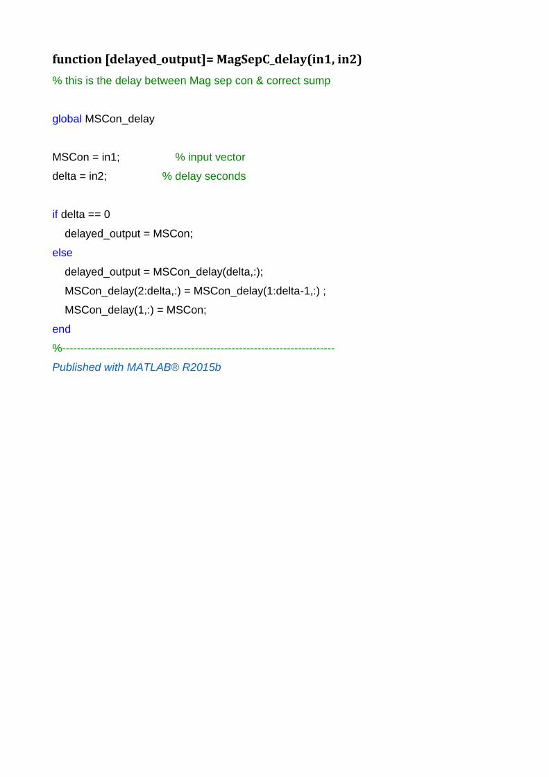
function [delayed_output]= MagSepC_delay(in1, in2)

% this is the delay between Mag sep con & correct sump

global MSCon_delay

MSCon = in1; % input vector


if delta == 0

delayed_output = MSCon;

else

delayed_output = MSCon_delay(delta,:);

MSCon_delay(2:delta,:) = MSCon_delay(1:delta-1,:) ;

MSCon_delay(1,:) = MSCon;

end

%--------------------------------------------------------------------------



function [delayed_output]= MagSeps_feed_delay(in1, in2)



from_Dil = in1; % input vector


if delta == 0

delayed_output = from_Dil;

else

delayed_output = from_Dil_delay(delta,:);

from_Dil_delay(2:delta,:) = from_Dil_delay(1:delta-1,:);

from_Dil_delay(1,:) = from_Dil;

end

%--------------------------------------------------------------------------



function[Mag_sep_CV, Mag_sep_TV] = MagSepVec2(Mag_sep_FV)

%--------------------------------------------------------------------------

%

% MAGNETIC SEPARATOR MODEL

%

%--------------------------------------------------------------------------

%

% Inputs: feed component vector [C W M NM T]

% Outputs: component vectors for concentrate & tails [C W M NM T]

Density_vector = [1.5 1.0 4.80 1.5]; % component densities

Mag_sep_feedV = Mag_sep_FV(5); % total m3/s

if Mag_sep_feedV <= 0

Mag_sep_feedV = 0.001;

end

Mag_sep_compsM =Mag_sep_FV(1:4) .* Density_vector(1:4); % CWMN mass t/s

Mag_sep_feedT = sum(Mag_sep_compsM); % total tps

if Mag_sep_compsM (4) <= 0

Mag_sep_compsM (4) = 0.001;

end

if Mag_sep_feedT <= 0

Mag_sep_feedT = 0.001;

end

M2NM = Mag_sep_compsM(3) / Mag_sep_compsM(4); % mags to non-mags

if M2NM <= 0

M2NM = 0.001;

end

Mass_pcS = 100*(Mag_sep_compsM(3) + Mag_sep_compsM(4))...

/ Mag_sep_feedT; % m% solids in feed

if Mass_pcS > 20

Mass_pcS = 20;

end

%Mag_losspc = (1 + 2.7 * M2NM ^-0.7) * (Mag_sep_feedV*3600)^-0.13...

% * Mass_pcS^0.12;

Mags_recpc = 99.9; %100 - Mag_losspc;

%NM_entrain = (4.5 * (100 * Mag_sep_compsM(4)/ Mag_sep_feedT)^-0.23) * ...

% (100 * Mag_sep_compsM(3) / Mag_sep_feedT)^0.96; % entrain %

NM_entrain = 25.0;

% assemble mag product vector & total m3/hr

Mag_sep_CV(1) = Mag_sep_FV(1) * 0.25;

Mag_sep_CV(2) = Mag_sep_FV(2) * 0.25;

Mag_sep_CV(3) = Mag_sep_FV(3) * Mags_recpc/100;

Mag_sep_CV(4) = Mag_sep_FV(4) * NM_entrain/100;

Mag_sep_CV(5) = sum(Mag_sep_CV(1:4));

% assemble mag tails vector & total m3/hr

Mag_sep_TV = Mag_sep_FV - Mag_sep_CV;



function [delayed_output]= MSCon_delay(in1, in2)

% this is the delay between Mag sep con & correct sump

global MSCon_delay

yo

MSCon = in1; % input vector


delayed_output=MSCon_delay(delta,:)

MSCon_delay(2:delta,:) = MSCon_delay(1:delta-1,:)

MSCon_delay(1,:)=MSCon

%--------------------------------------------------------------------------



function[RD]=Nucleonic(in1, in2)

% inputs: in1 vector of components of correct medium output C W M NM T

% in2 RD from last measurement

%

% outputs: new RD

%

%--------------------------------------------------------------------------

time_c =0.01; % filter time constant

density_vec = [1.5 1 4.8 1.5]; % component densities

to_Deslime = in1;

RD_old = in2;

if to_Deslime(3) <= 0 % check there is magnetite

to_Deslime(2) = 2; % in start up delay

to_Deslime(3) = 0.3; % so force an RD of 1.5ish

to_Deslime(5) = 2.3;

end

Massvec = to_Deslime(1:4) .* density_vec ; % component masses

RD_calc = sum(Massvec) / to_Deslime(5); % sum the masses / volume

RD = time_c * RD_calc + (1 - time_c) * RD_old; % filter



function[PV, Isum] = PI2(in1, in2, in3, in4, in5)

MV = in1; % measured RD

MV(MV <= 0)= 1.52; % default startup measured RD

SP = in2; % RD setpoint

Kp = in3; % proportional gain

Ki = in4; % integral time

Isum = in5; % integral

Error = MV - SP; % error

shift_Isum = Isum(1:9); % push the Isum vector down one

Isum(1) = Error;

Isum(2:10) = shift_Isum;

Int = sum(Isum)/10; % integral sum

PV = Kp * Error + Ki * Int; % control output



function[Rinse_vol, Rinse_W_2dil, water_OS, N] = Rinsepd2(in1, in2, in3,

in4)

%--------------------------------------------------------------------------

%

% RINSE SCREEN MODEL

%

%--------------------------------------------------------------------------



%

% inputs: in1 the medium vol to rinse m3/hr

% in2 total volume of rinse water m3/hr

% in3 coarse particles to rinse screen tph

% in4 area of rinse screen m2

%

% output: rinse volume m3/hr

%

%--------------------------------------------------------------------------

Q_to_rinse = in1; % vol of medium to rinse screen

Rinse_water = in2; % volume of rinse water used m3/hr

Coarse = in3; % tonnage of coarse particles to rinse tph

Rinse_area = in4; % area of rinse screen m2

% per cent mass (of the overflow stream) of the rinse water remaining

% with coarse particles

rem_water = 20; % can be adjusted but typical of end screen moisture %

% calculation, this is for two screens

water_OS = (Coarse * rem_water/100)/(1 - rem_water/100);

Rinse_W_2dil = Rinse_water - water_OS;

Rinse_vol = Q_to_rinse + Rinse_water - water_OS; % m3/hr through screen

N= (0.67 *((Q_to_rinse + Rinse_water)/Rinse_area)^0.66)/...

(Coarse / Rinse_area)^0.62;



function[Rinse_vol, Rinse_W_2dil, water_US, N] = RRinse(in1, in2, in3, in4)

%--------------------------------------------------------------------------

%

% RINSE SCREEN MODEL

%

%--------------------------------------------------------------------------



%

% inputs: in1 the medium vol to rinse m3/hr

% in2 total volume of rinse water m3/hr

% in3 coarse particles to rinse screen tph

% in4 area of rinse screen m2

%

% output: rinse volume m3/hr

%

%--------------------------------------------------------------------------

Q_to_rinse = in1; % vol of medium to rinse screen

Rinse_water = in2; % volume of rinse water used m3/hr

Coarse = in3; % tonnage of coarse particles to rinse tph

Rinse_area = in4; % area of rinse screen m2

% per cent mass (of the overflow stream) of the rinse water remaining

% with coarse particles

rem_water = 20; % can be adjusted but typical of end screen moisture %

water_US = (Coarse * rem_water/100)/(1 - rem_water/100);

Rinse_W_2dil = Rinse_water - water_US;

Rinse_vol = Q_to_rinse + Rinse_water - water_US; % m3/hr through screen

N= (0.67 *((Q_to_rinse + Rinse_water)/Rinse_area)^0.66)/...

(Coarse / Rinse_area)^0.62;

function [delayed_output]= to_MagSeps (in1, in2)



from_Dil = in1; % input vector


delayed_output=from_Dil_delay(delta,:);

from_Dil_delay(2:delta,:) = from_Dil_delay(1:delta-1,:);

from_Dil_delay(1,:)=from_Dil;

%--------------------------------------------------------------------------



function [delayed_output]= to_Wing_delay(in1, in2)



to_Wing = in1; % input vector


delayed_output=to_Wing_delay(delta,:);

to_Wing_delay(2:delta,:) = to_Wing_delay(1:delta-1,:) ;

to_Wing_delay(1,:)= to_Wing;

%--------------------------------------------------------------------------



function [delayed_output]= Wing_delay(in1, in2)



to_Wing = in1; % input vector


if delta == 0

delayed_output = to_Wing;

else

delayed_output=to_Wing_delay(delta,:);

to_Wing_delay(2:delta,:) = to_Wing_delay(1:delta-1,:) ;

to_Wing_delay(1,:) = to_Wing;

end

%--------------------------------------------------------------------------



function[Wtank_level,seal_level,W_overflow,Tankvol,Sealvol]=...

wing_tankVec(in1,in2,in3,in4,in5,in6)

% inputs 1 - 5 are vectors [C W M NM T]

% inputs: in1 (to_wing) coal & medium from deslime m3/s

% in2 (from_DR_drain) drain medium from DR screens m3/s

% in3 (DMCfeedvol) the volume pumped out based on the head m3/s

% in4 (tankvol_old) the existing volume in the coal side m3

% in5 (sealvol_old) the existing volume in the seal side m3

% in6 fraction of drain medium to seal side

%

% outputs: tank_level level on coal side m

% seal_level level on seal side m

% W_overflow overflow to CM sump m3/s vector [C W M NM T]

% updated tankvol_old m3/s vector [C W M NM T]

% update sealvol_old m3/s vector [C W M NM T]

%

%--------------------------------------------------------------------------

dorifice=0.31; % orifice diameter in metres

a = (pi * dorifice^2)/4; % a = orifice opening area in m^2

C=0.6; % constant for round orifice

g=9.81; % acceleration due to gravity

to_wing = in1;

to_wing(to_wing < 0) = 0;

from_DR_drain = in2;

from_DR_drain(from_DR_drain < 0) = 0;

DMCfeedvol = in3;

DMCfeedvol(DMCfeedvol < 0) = 0;

Tankvol_old = in4;

Tankvol_old(Tankvol_old < 0) = 0;

Sealvol_old = in5;

Sealvol_old(Sealvol_old < 0) = 0;

y = in6;

% get height in coal side from volume (relative to tank bottom)

V = [0.000 0.100 0.200 0.300 0.400 0.500 0.600 0.700 0.800 0.900 1.000...

1.022 1.042 1.101 1.164 1.228 1.295 1.364 1.434 1.507 1.582 1.659...

1.737 1.817 1.899 1.983 2.069 2.156 2.245 2.335 2.427 2.521 2.616...

2.654 2.660 2.757 2.854 2.951 3.049 3.146 3.243 3.340 3.437 3.535...

3.632 3.729 3.826 3.923 4.021 4.118 4.215 4.312 4.409 4.507 4.604...

4.701 4.798 4.895 4.993 5.090 5.187 5.284 5.381 5.479 5.576 5.673...

5.770 5.867 5.965 6.062 6.159 6.256 6.353 6.451 6.548 6.645 6.742...

6.839 6.898];

H = [0.000 0.086 0.171 0.257 0.343 0.429 0.514 0.600 0.686 0.772 0.857...

0.876 0.893 0.941 0.987 1.031 1.074 1.116 1.156 1.196 1.234 1.271...

1.308 1.344 1.379 1.413 1.446 1.479 1.512 1.543 1.574 1.605 1.635...

1.647 1.650 1.700 1.750 1.800 1.850 1.900 1.950 2.000 2.050 2.100...

2.150 2.200 2.250 2.300 2.350 2.400 2.450 2.500 2.550 2.600 2.650...

2.700 2.750 2.800 2.850 2.900 2.950 3.000 3.050 3.100 3.150 3.200...

3.250 3.300 3.350 3.400 3.450 3.500 3.550 3.600 3.650 3.700 3.750...

3.800 3.830];

Sump_vol = Tankvol_old(5);

Sump_vol(Sump_vol > 6.898) = 6.898;

Wtank_level = spline(V, H, Sump_vol);

% get height in seal side from seal volume (relative to tank bottom)

Seal_vol = Sealvol_old(5);

if Seal_vol<=0

seal_level=2.701; % height to base of seal leg

elseif Seal_vol>0 && Seal_vol<=3.043; % partially full

seal_level = (Seal_vol + 3.8909)/1.44;

elseif Seal_vol > 3.043

seal_level = 4.815; % max height of seal leg

end

%----------------------------------------------------------------------

% ORIFICE CALCULATION

% Delta P equals the height of seal leg minus tank level

% if DeltaP is negative then flow reverses UP the seal leg

DeltaP = seal_level - Wtank_level; % pressure drop across the orifice

if DeltaP < 0

k=-1;

else

k=1;

end

% vol flow rate through the orifice plate in the seal leg, m3/s

Qorifice(5) = k * C * a * sqrt(2*g*abs(DeltaP));

%----------------------------------------------------------------------

% WING TANK LOGIC

% fill the wing tank, Tankvol is the coalside volume, Sealvol is the

% seal leg side volume

Seal = Sealvol_old + from_DR_drain .* y; % seal side components

Qorifice = (Seal ./ Seal(5)) .* Qorifice(5); % components

Sealvol= Sealvol_old + from_DR_drain .* y - Qorifice;

Tankvol = Tankvol_old + to_wing + (1-y)*from_DR_drain ...

- DMCfeedvol + Qorifice ;

% seal side overflowing?

if Sealvol(5) < 1.742

W_overflow = [0 0 0 0 0]; % not overflowing

elseif Sealvol(5) >= 1.742 % overflowing

W_overflow = (y .* from_DR_drain - Qorifice);

end

Sealvol= Sealvol_old + y*from_DR_drain - Qorifice - W_overflow;

%--------------------------------------------------------------------------



7.4 Appendix 4: Published Papers



Istanbul, Turkey.



Circuit, 15th Australian Coal Preparation Conference Proceedings 14-18th Sept 2014,

Gold Coast, Australia







O’Brien,M., Firth,B., Holtham,P., Hu,S., Scott,N., Burger,A., Optimisation and Control of

Dense Medium Cyclone Circuits, International Coal Preparation Congress, July 2016, St

Petersburg, Russia

7.5 Appendix 5: Standard Deviations from Tracer Residence Times

Additional results below were included for the tracer residence times. The standard deviations are included here, however it is important to note that in some cases, the value of this measurement is low. In situations where more than one pathway could be taken by a particle, the standard deviation was high. This makes logical sense because the data in those cases is multi-modal and it is reasonable to expect high variation given that the routes taken aren’t necessarily the same.

Test Residence time From Residence time to Average Min Max SD

A Desliming Screen Drain & Rinse Product 1 00:57 00:37 01:41 0.0001

Desliming Screen Drain & Rinse Product 2 01:00 00:36 01:56 0.0002

Desliming Screen Drain & Rinse Rejects 01:02 00:43 02:11 0.0002

Desliming Screen Drain & Rinse Overall 01:01 00:36 02:11 0.0002 For the desliming screen the standard deviation was as follows and suggested that there is low variation in travel times of the data. For the other areas tested, standard deviations ranged as follows:


B DMC Overflow/Underflow Drain & Rinse Screen 00:20 00:15 00:26 0.00003 This standard deviation suggested that there is low variation in travel times of the data. In reality, the particles travelled a total of approximately 10 metres with no chance of deviation.


C&D Drain underpan Drain and Rinse Screen 02:36 00:43 29:06 0.0029 Tracers were placed in drain under-pans and collected at the coarse overflow launder on the drain and rinse screens. These particles followed the medium and substantial variation was evident in the data.


E Feed Weigher Drain and Rinse Screen 02:25 02:00 03:27 0.0002 These tracer particles entered at the feed weightometer and followed the coal through the process. There was little opportunity for particles to be delayed and all appear to have gone straight through the DMC without deviating into the medium stream.


F Magnetic Separator Drain and Rinse Screen 09:50 01:10 39:36 0.0070

These particles entered at the concentrate launder of the magnetic separator and then routed through the correct medium sump. Some particles took considerable time to flush through the system suggesting that they may have stayed with the medium for quite a long time before joining the coarse coal. The standard deviations reflect this variation.


G Deslime Water Sump Drain and Rinse Screen 08:37 02:09 35:51 0.0072 Particles placed into the Deslime water make-up sump appeared to have taken varied routes or held up in the system before entering the coarse coal pathway. The likelihood that particles just settled out and sat in the bottom of this tank for a while cannot be discounted as the relative density of the fluid (water) to the particles is considerably different. As a consequence, standard deviation was poor and the minimum and maximum times also suggest wide variation from one particle to the next.


H Crusher Feed Drain and Rinse Screen 01:55 01:36 02:25 0.0002 Predictably, these particles followed the coarse coal route, having been introduced to the coal stream at the feed to the crusher. Standard deviation is relatively low as there is very little chance of particles not following the coal stream unless they were to raft up into the seal leg of the wing tank and overflow to the correct medium sump. On the day of the testwork, it is suggested that rafting in the wing tank was highly unlikely and no evidence of rafting was found.


I Wing Tank Overflow Drain and Rinse Screen 06:53 01:23 31:48 0.0046 Particles entering at the wing tank overflow mimicked the action of a rafting particle. They were placed in the overflow which reported to the correct medium sump and these particles had multiple routes which they could follow. Judging by the minimum time, some particles went straight through the correct medium pump and directly back to the wing tank, however others to a far longer route, either settling out in the correct medium sump, or following the bleed line across to the dilute sump before returning in a water stream back to the start of the process. (The magnetic separator effluent line returns to the deslime water make-up sump.) Standard deviations were poor in this case which is not surprising.

master of business administration bachelor of chemical ...683425/s42824822_phd... · a thesis...

Documents