master thesis 08042014 - final public
TRANSCRIPT

Name: Jesse Leeuwendal First supervisor: Ir. Henk Kroon Student nr.: s0145203 Second supervisor: Dr. Berend Roorda Study: Ind. Engineering & Management Date: March 2013
Master Thesis – Public Version
Analysing & Forecasting Nordic Electricity Prices Utilizing technical and fundamental analyses to develop long-‐term
forecasts for the system price
March 2013 Jesse Leeuwendal


Analysing & Forecasting Nordic Electricity Prices Utilizing technical and fundamental analyses to develop long-‐term forecasts for the system price
Author: Jesse Leeuwendal Study: Master Financial Engineering and Management University of Twente Student number: s0145203 Telephone: 06-‐23917689 E-‐mail: [email protected] Organisation: Address: Supervisors X: Supervisors University: Ir. Henk Kroon
Lecturer at the University of Twente Dr. Berend Roorda
Associate Professor of Financial Engineering at the University of Twente
Date of publication: 27-‐03-‐2013


5
Preface This master thesis is the result of my internship at the Structured Finance Energy Origination department of X, London, United Kingdom. This research was part of my graduation assignment for my Master study Financial Engineering & Management at the University of Twente. For conducting this research and presenting this report, I would like to specially thank the following people: Dhr. Henk Kroon for supervising the process of my internship and providing useful feedback to successfully fulfil this assignment; for being my supervisor at X, providing feedback on my thesis and by aiding and involving me in the business of originating and structuring renewable energy projects in Europe; for originating my internship and providing guidelines and assistance during the process of conducting this research, while in the meantime involving me in several business deals; My brother Jorn Leeuwendal for introducing me to X, reviewing this research and providing useful insights in the business of renewable energy project financing; My girlfriend, friends and family who supported my during the 6 months abroad and provided the necessary ‘quality’ time when they came over to pay a visit to London; and all employees of the Structured Finance Energy Origination and Portfolio Management department of X for their help during the past 6 months and for making it a very pleasant and extremely learning experience.
Jesse Leeuwendal, 27 March 2013 Sint Nicolaasga, The Netherlands


INDEX
EXECUTIVE SUMMARY .................................. 9 SAMENVATTING ........................................... 11 CHAPTER 1 – INTRODUCTION ................. 13 CHAPTER 2 – THEORETICAL BACKGROUND ............................................... 15 2.1 RENEWABLE ENERGY PROJECT FINANCE . 15 2.2 SWEDISH & NORWEGIAN MARKET ............ 16 2.2.1 Nordic Electricity market ............... 16 2.2.2 Generation Nordic market ............. 17 2.2.3 Renewable Energy projects in Norway and Sweden ..................................... 18
2.3 CONCLUSION .................................................. 19 CHAPTER 3 – RESEARCH PROBLEM ....... 21 3.1 PROBLEM STATEMENT ................................. 21 3.2 RING FENCING / LIMITATIONS ................... 22
CHAPTER 4 – LITERATURE REVIEW ...... 23 4.1 ELECTRICITY PRICE BEHAVIOUR ............... 23 4.2 KEY FACTORS ................................................. 24 4.3 ELECTRICITY PRICE FORECASTING LITERATURE .......................................................... 25 4.4 CONCLUSION .................................................. 27
CHAPTER 5 – MODEL METHODOLOGY . 29 5.1 FORECAST METHODOLOGY ......................... 29 5.2 FORECAST MODELS ....................................... 29
CHAPTER 6 – MODEL FRAMEWORK ...... 33 6.1 TECHNICAL ANALYSIS .................................. 33 6.1.1 Data evaluation ................................... 33 6.1.2 Statistical Analysis of Prices .......... 33 6.1.3 Conclusion .............................................. 36
6.2 FUNDAMENTAL ANALYSIS ........................... 36 6.2.1 Data Evaluation .................................. 36 6.2.2 Hypotheses ............................................. 36 6.2.3 Analysis ................................................... 37 6.2.4 Conclusion .............................................. 41
CHAPTER 7 – FRAMEWORK APPLICATION ................................................ 43 7.1 APPROACH ..................................................... 43 7.2 TECHNICAL FORECAST MODELS ................ 44 7.2.1 Models presentation ......................... 44 7.2.2 Models forecast ................................... 46
7.3 FUNDAMENTAL FORECAST MODELS ......... 46 7.3.1 Models presentation ......................... 47 7.3.2 Models forecast ................................... 48
7.4 MERGED FORECAST MODELS ...................... 49 7.4.1 Models presentation ......................... 49 7.4.2 Models forecast ................................... 50
7.5 CONCLUSION .................................................. 51 CHAPTER 8 – PROJECT FINANCING PERSPECTIVE ................................................ 53 8.1 SCENARIOS ..................................................... 53 8.2 EXTERNAL FACTORS FORECAST ................. 53 8.2.1 Oil .............................................................. 54 8.2.2 Interconnection .................................. 54 8.2.3 Demand .................................................. 55
8.3 MODEL APPLICATION ................................... 56 8.4 CONCLUSION .................................................. 58
CHAPTER 9 – CONCLUSION, DISCUSSION & RECOMMENDATIONS .............................. 59 9.1 CONCLUSIONS ................................................ 59 9.1.1 Analysis ................................................... 59 9.1.2 Forecast .................................................. 60
9.2 DISCUSSION .................................................... 60 9.3 RECOMMENDATIONS .................................... 62
REFERENCES .................................................. 65 APPENDICES .................................................. 69


9
Executive Summary The goal of this research is to gain knowledge about the behaviour of the electricity price in Norway and Sweden. The gained knowledge is used to support to decision process in originating and structuring renewable energy projects in these countries. In order to do so, the key factors influencing the electricity price in these countries are analysed and forecasting models are developed to predict future electricity prices over a 15-‐year time period. Due to the long-‐term nature of renewable energy project financing, the analysis and forecast of electricity prices is based on monthly prices. The different monthly electricity prices in Norway and Sweden are statistically analysed during 2000-‐2012. First conclusion is that the so-‐called system price is a good indicator for all other prices and is therefore the only price to be further analysed and forecasted in this research. The system price is subject to high volatility, non-‐normality, daily, weekly and yearly seasonal cycles and price spikes. Furthermore, the system price is mean-‐reverting, indicating that the price reverts back to its mean over time. To analyse which key factors influence the system price, the research utilises time-‐series analysis to construct several models, which try to replicate the historical behaviour of the system price. Based on literature research and discussions with experts, several external factors are indicated to have potential influence on the electricity price. The time-‐series analysis and examination of the performance of the constructed models leads to the conclusion that the main external key factors influencing the system price in Norway and Sweden are: 1) Oil; 2) Electricity demand; and 3) Interconnection of electricity between the Nordic and non-‐Nordic countries. Besides these external factors, the historical electricity prices of one and two months in the past also have a significant influence on the current monthly electricity price. The time-‐series analysis develops multiple models replicating the behaviour of the system price. The best performing model is utilised to construct a 15-‐year out-‐of-‐data forecast for the system price, i.e. for the years 2013 till 2027. This model is based on an ARMA structure and utilises the historical electricity price of one month in the past and the external factors oil, demand and interconnection to construct a 15-‐year monthly electricity price forecast. The forecast includes four different scenarios, leading to the conclusion that the electricity price in 2027 will be between the low scenario (circa €18,-‐ per MWh) and the medium scenario (circa €40,-‐ per MWh). Note that these prices are not indexed by inflation. Furthermore, three out of the four scenarios indicate a stable or declining trend for the system price over the upcoming 15 years. The analysis and forecast of the electricity prices in Norway and Sweden develop valuable knowledge for X. The model forms a suitable alternative for simulation forecasting models. The analysis and forecasting model can support future renewable energy project financing opportunities in Norway and Sweden by offering in-‐depth knowledge about the market and the electricity price in order to make informed decisions. An overview of all conclusions and recommendations can be found in chapter 9, page 59.


11
Samenvatting Het doel van dit onderzoek is om kennis te vergaren omtrent het gedrag van de elektriciteitsprijs in Noorwegen en Zweden. Deze kennis kan worden gebruikt ter ondersteuning van het proces van het ontwikkelen en het financieel structureren van duurzame energie projecten in deze landen. Om dit te bewerkstelligen wordt er onderzocht welke factoren de elektriciteitsprijzen in Noorwegen en Zweden beïnvloeden en worden er voorspellingsmodellen ontwikkeld om de toekomstige elektriciteitsprijzen te berekenen over een periode van 15 jaar. Vanwege het lange-‐termijn karakter van duurzame energie project financiering zijn de analyse en voorspelling van elektriciteitsprijzen gebaseerd op maandelijkse prijzen. De verschillende maandelijkse elektriciteitsprijzen in Noorwegen en Zweden zijn statistisch geanalyseerd gedurende 2000-‐2012. De eerste conclusie is dat de zogenoemde ‘system price’ een goede indicator is voor alle andere prijzen en vandaar als enige verder wordt geanalyseerd en voorspeld in dit onderzoek. De ‘system price’ is erg volatiel, heeft geen normale verdeling, is onderhevig aan dagelijkse, wekelijkse en jaarlijkse cycli en heeft prijspieken. Ook heeft de ‘system price’ een bepaalde gemiddelde waarde en heeft het de neiging terug te gaan naar deze gemiddelde waarde. Dit onderzoek maakt gebruik van tijdreeks analyse om te bepalen welke factoren de ‘system price’ beïnvloeden en om verschillende modellen te ontwikkelen welke het historische gedrag van de ‘system price’ proberen te benaderen. Gebaseerd op literatuur onderzoek en discussies met experts zijn er verscheidene externe factoren aangemerkt welke een significante invloed zouden kunnen hebben op de elektriciteitsprijs. De tijdreeks analyse en het onderzoeken van de prestaties van de ontwikkelde modellen leiden tot de conclusie dat de volgende externe factoren een significante invloed op de ‘system price’ in Noorwegen en Zweden hebben: 1) Olie; 2) Vraag naar elektriciteit; 3) Import en export van elektriciteit tussen Noorse landen en niet-‐Noorse landen. Naast deze externe factoren hebben ook de historische elektriciteitsprijzen van één en twee maanden in het verleden een significante invloed op de huidige maandelijkse elektriciteitsprijs. De tijdreeks analyse ontwikkelt meerdere modellen welke het gedrag van de ‘system price’ benaderen. Het best presterende model wordt gebruikt om een voorspelling te doen voor de ‘system price’ over 15 jaar, d.w.z. over een periode van 2013-‐2027. Dit model is gebaseerd op een ARMA structuur en maakt gebruikt van de historische elektriciteitsprijs van één maand in het verleden en de externe factoren olie, elektriciteitsvraag en import / export van elektriciteit. De voorspelling bestaat uit vier verschillende scenario’s welke leiden tot de conclusie dat de elektriciteitsprijs in 2027 tussen het lage scenario (circa €18,-‐ per MWh) en het middelste scenario (circa €40,-‐ per MWh) zal liggen. Deze prijzen zijn niet geïndexeerd met inflatie. Daarnaast vertonen drie van de vier scenario’s een stabiele of dalende trend voor de ‘system price’ over de aankomende 15 jaar. De analyse en voorspelling van de elektriciteitsprijzen in Noorwegen en Zweden hebben waardevolle kennis ontwikkel voor X. Het model vormt een geschikt alternatief voor simulatie voorspellingsmodellen. De analyse en het voorspellingsmodel kunnen toekomstige kansen voor het financieren van duurzame energie projecten ondersteunen door het aanbieden van kennis over de markt en de elektriciteitsprijs zodat geïnformeerde beslissingen gemaakt kunnen worden. Een overzicht van alle conclusies en aanbevelingen is te vinden in hoofdstuk 9, pagina 59.


13
Chapter 1 – Introduction This master thesis is executed on behalf of X, London. X is the leading universal bank in the north of X. It supports inter alia the public sector in municipal financing and assumes the responsibilities of a central bank for the savings in this part of X. X’s headquarters are situated in X and as an internationally operating commercial bank it also has offices in significant financial and trading centres such as London, New York and Singapore. The problem this research focuses on is identified by X’s Structured Finance Energy Europe department. Structured Finance Energy Europe is a financer of projects in the area of renewable energy. Their extensive know-‐how of this market is based upon a large and long existing renewable energy portfolio. The department provides the following services with a bi-‐national team in Hanover and London, with similar units in New York and Singapore:
1. Advisory: Support their customers in diverse issues right from the earliest phases of the project;
2. Arranging: X is a lead financer in the area of renewable energies and has diverse mandates as the lead arranger and leader of bank consortiums;
3. Structuring: Specially tailored financing to each customer’s own needs in order to optimise the entire financing structure under consideration of all aspects.
The aim of this research is to support the Structured Finance Energy department of X to understand the volatility of the electricity prices in the Nordic market, as further explained in chapter 3. This will be done by analysing and forecasting the electricity price in the Nordic markets. An in-‐depth analysis and long-‐term forecast of electricity prices give X guidelines to tackle this problem by offering insight in the behaviour and future development of the price. The contribution of this research with regard to similar investigations is that it focuses on long-‐term analysing and forecasting of an electricity price. Instead on investigating the behaviour of daily or weekly prices, this research aims to analyse the monthly prices. Based on this analysis long-‐term forecast models are presented, predicting the electricity price over a 15-‐year period. This is done by a technical and fundamental analysis and corresponding econometric models. The few other long-‐term forecasting investigations utilise simulation models to achieve a similar goal. The research is organised as follows: Chapter two introduces the Norwegian and Swedish electricity markets and the business of renewable energy project finance. These topics are discussed briefly (and by no way comprehensively), but offer a common knowledge to comprehend the remainder of the research. Chapter three introduces the research problem and the relevant literature in addressing this problem is discussed in chapter four, focussing on electricity price behaviour and electricity price forecasting literature. Chapter five explains the methodology adopted by this research for analysing and forecasting the electricity price. The technical and fundamental analyses are introduced in chapter 6 and utilised in chapter 7 to construct multiple forecasting models and to determine the forecasting ability of these models. In chapter 8 the best performing model will be used to forecast the electricity price over a 15-‐year period. Conclusions, a discussion and recommendations are presented in chapter 9.


15
Chapter 2 – Theoretical Background This chapter will provide the necessary background information to understand the research problem and therefore the remainder of the research. The topics introduced here are renewable energy project finance and the Norwegian and Swedish electricity market. The introduction in chapter 1 about X and the aim of this research clarify the inclusion of just the two topics of renewable energy project finance and the Norwegian and Swedish electricity market.
2.1 Renewable Energy Project Finance There are two distinctive features of the business of the Structured Finance Energy Origination department in which this research finds its origination, i.e. Renewable Energy and Project Finance. In this paragraph both topics will be briefly discussed, thereby developing a common, basic knowledge of the background of the research problem.
Renewable Energy Renewable energy generation is electricity generated by making use of infinite, natural resources, opposite to non-‐renewable sources such as fossil fuels. These non-‐renewable sources are consumed more rapidly than they are created and draw on finite resources that will eventually seize to exist. Renewable energy generation uses sources such as the sun, wind, rain, waves and the earth. Since X focuses on wind and solar technologies, only a short summary of these renewable techniques is provided below. The sun’s energy can be used for heating but also for generating electricity. The main technologies for transforming sunlight towards electricity are concentrated solar power (CSP) and photovoltaic solar cells (PV) integrated in so-‐called solar panels. These techniques can be used on a small scale (e.g. several solar panels on rooftops of houses) or on a large scale. Over the last few years the cost of photovoltaic solar cells has decreased while the efficiency has increased significantly making the technology more competitive with conventional electricity sources. PV is seen by X as one of the most mature and proven renewable energy technologies and is therefore one of the technologies it engages in. Most projects X finances utilise another renewable energy technology, being wind power. Wind power makes use of wind turbines to convert the energy of the wind into some other sort of energy, e.g. kinetic energy. Wind power is in fact also indirectly powered by the sun, i.e. the sun’s heat drives the wind that produces energy that is captured with wind turbines (Kaygusuz & Kaygusuz, 2002). The wind power that this research is focused on is on the wind power technology transforming the wind power into electricity. These turbines can be situated on land (onshore wind) or in a lake or sea (offshore wind). Whilst onshore wind is a mature and proven technology, offshore wind is still subject to more risks and obstacles. In order to stimulate their development and secure their participation in a new restructured electricity industry, support mechanisms have been created for renewable energy generation projects (Falconett & Nagasaka, 2010). The two most prominent support mechanisms are: 1) Feed-‐in-‐Tariffs; 2) Renewable Energy Certificates. Feed-‐in-‐Tariffs involve an obligation for electric utility companies to purchase the electricity produced by renewable energy generators at a tariff determined by the public authorities and guaranteed for a specific period of time (e.g. 15-‐20 years) (Menanteau, Finon, & Lamy, 2003). This scheme is successfully employed in countries such as Germany, France and Denmark. In a Renewable Energy Certificates scheme a fixed quota of electricity sold by suppliers on the electricity market has to be generated by renewable energy technologies. The suppliers comply with this obligation by buying renewable energy certificates. These Renewable Energy Certificates are issued to the renewable energy generators and since the suppliers are obliged to meet the quota, there is demand for these certificates. So the renewable energy generator benefits from generating renewable energy in two ways: By selling the electricity on the

16
network at the market price, and by selling certificates on the green certificates market (Menanteau et al., 2003).
Project Finance Project financing is, as the term indicates, basically the financing of projects. These projects could be of any kind, e.g. infrastructure projects such as schools, hospital and bridges or renewable energy projects, such as wind farms and solar parks. The specific aspect of project financing is that it is based on non-‐recourse or semi-‐recourse financing. This means that the financing is based upon the projected cash flows of the project rather than the balance sheet of underlying sponsors. In other words, the cash flows of the project should be able to repay the loan and accompanying interest on itself. It is called non-‐recourse because the loan is only secured by the project itself and in case of a default the lender’s recovery is limited to that collateral. To protect the other assets of a sponsor from a default of the project, it is common in project finance to create a special purpose vehicle (SPV) for each project. Stable cash flows form the basis for project finance and are formed by the operational revenues and costs of a renewable energy project. Revenues basically consist of the price paid per megawatt hour (MWh) times the produced electricity, plus additional revenues generated by the support mechanisms explained earlier. The costs vary per project and consist among others of operation and maintenance (O&M) contracts, land leases and insurance costs. It is common in renewable energy project finance that several costs are fixed for multiple years, e.g. by a 10 or 15-‐year O&M contract and long-‐term land lease contracts. To secure revenues, Power Purchase Agreements1 (PPA) are used to guarantee that produced electricity will be sold. Since lenders are not keen on market price risk, the tenor of provided loans usually depends on the tenor of the underlying contracts, which determine the cash flows for the future years. It is common in project finance that the tenor of the loan is shorter than the lifetime of the project and the applicable support mechanism in order to include a buffer. In general, the cash flows of the projects should be predictable in order for lenders to provide the financing.
2.2 Swedish & Norwegian market The main markets of interest for this research are the Swedish and Norwegian market. Both electricity markets are part of the Nordic electricity market, along with the Danish and Finnish electricity market. The electricity price is determined using a Nordic wide exchange market called Nord Pool. Since these markets are all combined, the remainder of this paragraph will mainly deal with the Nordic market in general instead of the Norwegian and Swedish markets on its own. When it is deemed necessary, additional information about the distinctive markets is provided.
2.2.1 Nordic Electricity market Norway and Sweden participate in the Nordic electricity market. This market was set up between 1991 and 2000 when the electricity markets of Denmark, Finland, Norway and Sweden were opened for competition in generation and retailing. One of the reasons for this was the widely held believe that increased competition would raise power industry efficiency to the benefit of the customers, provided that there are sufficient competitors in the market. The Nordic electricity consumption is relatively high compared to other countries. This is due to the high level of electric heating in combination with cold winters and a relatively high proportion of energy intensive industry (NordREG, 2012). This is especially the case for the Swedish, Norwegian and Finnish markets. The Nordic electricity grid has multiple connections to other countries. It is part of the transmission network in North-‐Western Europe and it combines the whole Nordic market to one synchronous power system (NordREG, 2012). The interconnection links run to Germany, Poland, Estonia, Russia and the Netherlands.
1 Contracts between generator and off taker including a certain price paid per MWh supplied for a fixed number of years.

17
Nord Pool The Nord Pool power exchange is the key trading institution in the Nordic electricity market. It is an ‘energy only’ spot market at which hourly electricity prices are determined in single price auctions (Amundsen & Bergman, 2006). The Nord Pool was the first international power market in the world and was established by Norway in 1993. In 1996 the Swedish and Norwegian markets merged into one market, while Finland, West Denmark and East Denmark joined the market in 1998, 1999 and 2000 respectively (Torghaban, Zareipour, & Le, 2010). Trading at Nord Pool is voluntary. Despite this voluntary character, the trade volumes at the Nord Pool have increased steadily over the past years and the total volume at Nord Pool traded in 2011 was about 78% of the total Nordic electricity consumption (NordREG, 2012). The other part is traded on a bilateral basis between generators and suppliers. The Nord Pool consists of three sub-‐markets, being the day-‐ahead market Elspot, the intra-‐day market Elbas and the financial market Eltermin. In the Elspot sub-‐market electricity is traded for the next day. In Elbas participants from Norway, Finland, Sweden, Denmark, Germany and Estonia can trade for the upcoming day after the Elspot market has closed (NordREG, 2012). At Nord Pool’s Eltermin forwards, futures and options are traded, such that buyers and generators can hedge the system price risk (Amundsen & Bergman, 2006). At the Elspot sub-‐market there is a distinction between the so-‐called ‘system price’ and ‘area prices’. At each hour a market-‐clearing price is determined based on the bids made by sellers and buyers of the electricity. The market-‐clearing price is called the system price and is based on the assumption that interconnection capacities are sufficient and therefore no bottlenecks are found in the transmission grid (Bergman, 2003). However, when one or several interconnectors become congested, the equilibrium area prices are computed using information about the location of the bidding units. These area prices then differ from the system price. In total there are six different areas in Norway, four areas in Sweden, two in Denmark and one area in Finland. This research focuses on the system price of the Elspot sub-‐market. One reason is that the system price forms the basis for the other area prices and is therefore a good indicator for these prices. Additional reasons for choosing the system price are discussed in chapter 6. Please keep in mind that the system price is the price determined by the equilibrium point between demand and supply independent of potential grid congestions and forms the basis for financial trades in the market.
2.2.2 Generation Nordic market The Nordic market has a variety of generation sources, being hydro, wind, nuclear and thermal power (NordREG, 2012). The figures of the generation capacity in the Nordic market are summarised in table 1. Hydro plays an important role in the generation of power since it represents almost all generation capacity in Norway, half of the generation capacity in Sweden, and more than 50% of the total Nordic generation capacity (NordREG, 2012). The second largest generation source in the Nordic market is thermal power generation consisting of Combined Heat and Power (CHP) plants. As the name suggests, these plants provide as well heat to houses / industries as electricity. It accounts for 31% of the total Nordic market power generation and acts as a so-‐called ‘swing-‐production’. This means that this capacity is used to balance the total production during the seasons when the level of hydropower generation in Norway and Sweden is low (NordREG, 2012). The fuels used for the CHP plants are coal, oil, gas and biofuels. The third largest power generation source is nuclear power. It has a share of 12% of the total Nordic generation capacity. Nuclear power plants are only situated in Sweden and Finland. The final part of 7% of the total generation capacity is provided by wind power, which has increased continuously during the last couple of years. The capacity in Sweden has grown by almost 34% in 2011 compared to 2010 and a lot of projects for new wind power generation are planned for the upcoming years (NordREG, 2012). The total installed generation capacity in the Nordic market is 98.414 MW and the total power generated during 2011 was 370 TWh (NordREG, 2012). Compared to 2010, approximately 3TWh was produced less in 2011 due to a decrease in demand. The Nordic Market Report

18
(2012) indicates weak economic outlook and warmer weather as reasons for the decrease in demand.
Denmark Finland Norway Sweden Nordic Region
Installed capacity (total) 13,540 16,713 31,714 36,447 98,414 Nuclear Power -‐ 2,716 -‐ 9,363 12,079 Other Thermal Power 9,582 10,651 1,062 7,988 29,283
Condensing Power 1,590 2,155 -‐ 1,623 5,368 CHP, District Heating 7,118 4,300 -‐ 3,551 14,969 CHP, Industry 674 3,362 -‐ 1,240 5,276 Gas Turbines etc. 200 834 -‐ 1,574 2,608
Hydro Power 9 3,149 30,140 16,197 49,495 Wind Power 3,949 197 512 2,899 7,557
Table 1: Installed Electricity Generation Capacity in the Nordic Region Source: NordREG (2012)
2.2.3 Renewable Energy projects in Norway and Sweden Besides high integration of hydro generation in Norway & Sweden, the markets also have numerous renewable energy projects of interest for X (mainly wind). A short overview of renewable energy projects financed in the past is provided in this part and the support mechanism in Norway and Sweden is introduced.
Projects Market research indicated that 700+ wind farms have been developed or are in the pipeline in Sweden alone (The Windpower, 2012). They range from small, single turbines (<1mw) to big wind farms (>100mw). Further research has been conducted to determine underlying assumptions and financial conditions on which these projects are structured. However, this specific data is not widely available. A bit of information about six projects has been retrieved from Project Finance Magazine (2012). Some interesting aspects of these projects are summarised below, although it should be noted that the information cannot be verified and validated:
1. Two projects financed in 2010 had a debt : equity ratio of 100 : 0, meaning that there is no equity invested in the project itself;
2. Several projects were financed by funds that were granted by a government or governmental institution. Together with low leverages (circa 65%), conservative wind assumptions (P95), and the inclusion of cash sweeps and high distribution lock-‐ups reduced the market risk for the lenders;
3. It is certain that at least one lender of a project used X as their market consultant. X has financed one project in Sweden in the past. The reasons for not having long term PPAs is that utilities also do not know how the price will develop and they are even more risk-‐averse than banks. Besides, the Nord Pool is very liquid so it is easy to trade electricity. The off-‐takers look at the futures being traded on this liquid market and since futures do not extend 5 years, they do not want to offer longer PPAs than this period. This research will develop alternative models for X to forecast the electricity price in Norway and Sweden.

19
Support System Norway and Sweden have a combined Renewable Energy Certificate Market. The certificates traded at this market are called Tradable Green Certificates (TGC) and are an example of the Renewable Energy Certificates introduced in paragraph 2.1. Producers of renewable energy receive a certificate for each MWh they produce. By selling these certificates, the producers receive an extra income in addition to the revenue made by selling the electricity itself. Producers are entitled to electricity certificates for a maximum period of 15 years. The system aims to promote the development of renewable electricity production and is technology neutral (Swedish Goverment, 2006). This latter means that cheap hydro generating technologies get the same amount of green certificates per produced MWh as more expensive technologies such as wind and solar. The cheaper renewable energy production technologies therefore have an advantage over the more expensive alternatives, which is also concluded by Unger and Ahlgren (2005). To create demand for these certificates, the governments have set a quota obligation. The quota obligation is an annual obligation for electricity suppliers to hold electricity certificates corresponding to their sale and use of electricity during the year (Swedish Goverment, 2006). The receivers of the certificates do not have the obligation to sell their certificates. They are allowed to ‘bank’ their certificates and sell them in future years. The banking of certificates can provide the demand elasticity to level out price fluctuations (Kildegaard, 2008). There is however a risk of oversupply of certificates due to overinvestment in renewable energy projects and/or a too low quota obligation. Oversupply results in a prolonged depression of certificates prices until the excess capacity is utilised (Kildegaard, 2008). In the Norwegian and Swedish market an oversupply of TGCs has been the case over the last few years.
2.3 Conclusion Opportunities for financing renewable energy projects were and are present in Norway and Sweden. The regimes are developed to protect the consumers for high electricity prices and are not developed to support the implementation of renewable energy. This stems from the fact that there is no floor price2 for the wholesale electricity price and for the price of tradable green certificates. In comparison, the support regime in Germany lets the consumer pay an extra price for electricity to support the renewable energy development directly. Based on historic deals the projects in this market already have lower leverage than commonly seen in renewable energy finance, i.e. 65% vs. 80-‐85%. Current market situations are expected to be similar to this lower range. Even though, the short-‐term PPAs expose the lender to market price risk. This research aims to analyse the behaviour of the market price and the key factors influencing the price and to develop a suitable forecast.
2 Minimum price determined by government or market to ensure fixed minimum revenue for projects.


21
Chapter 3 – Research Problem The previous chapter has provided the background information for the problem statement of this research. The problem X has encountered is stated in this chapter and a short explanation of how the problem will be tackled is given. The chapter ends with ring fencing and the limitations of the research. An important part of grasping the project context of this research is to understand the business the Structured Finance Energy department is participating in, i.e. project finance of renewable energy projects. As explained in chapter 2, project finance relies on the cash flows of the project itself. These cash flows are predicted by financial modelling at X and form the basis for the debt structuring. Along with the fact that the debt structuring is based on the cash flows, is that the financing is subject to tight covenants. These tight covenants translate in little room for error. Changes in cost and revenue assumptions in the financial model of a project have an impact on the cash flows and therefore the debt structuring of a project. Changes therefore impact the ability of a project to meet its liabilities with regard to repaying the lenders. The project financing of renewable energy with its specific characteristics is called ‘the product’ in the remainder of this research. The market subject to this research is the other part of the project context, i.e. Norway & Sweden. There are several specific features of these markets that have a big influence for project financing. First of all, there is a tradable green certificate system in place in order to support the development of renewable energy. The price of these certificates is very volatile and there is no floor price in place. Secondly, the electricity price in the markets is perceived as being very volatile. While it is common in most markets to have long term PPAs available (e.g. 15-‐20 years), that take away the complete or part of the volatility in the prices, in Norway & Sweden only PPAs for 5 years are available. To conclude, the Swedish & Norwegian markets have volatile electricity and certificate prices resulting in volatile revenues of renewable energy projects. As a consequence the cash flows of the projects are volatile.
3.1 Problem Statement Combining the context of project finance and of the markets, it can be seen that there is a mismatch: The traditional structure of project finance, with its long tenor, non-‐recourse, low margins (i.e. little room for error) does not suite a market in which the revenues are very volatile, which can result in too low cash flows for the project to meet its liabilities. This leads to the following problem statement: The current product (project finance of renewables) is not suitable for the Swedish & Norwegian
market. Instead of focussing on developing the product itself, the goal of this research is to gain insight in the electricity price behaviour. This is separated in two goals:
1. Analyse the key factors in Norway and Sweden that determine the electricity price behaviour;
2. Forecast the electricity price in Norway and Sweden for a long-‐term period in the future. Key factors influencing the electricity price provide insight in the volatility of the price. This developed knowledge will be used to forecast the electricity price in Norway and Sweden by developing different forecasting models. The data of these models can be used to determine if the risk of project financing in Sweden and Norway is acceptable and to develop a product that can be applied in these markets. Since project finance is very project specific it is impossible to develop a general product suitable for all Norwegian and Swedish projects. The development of a product itself is not the aim of this research. It merely provides the basic knowledge about the electricity price for X useful in future decision processes.

22
3.2 Ring fencing / Limitations This research is limited in its focus and its application. Reasons for doing so is to ensure that the research is relevant for the user and feasible to conduct in the given time period. This paragraph describes and explains the limitations of the research. First of all, the focus is only on the electricity price. The electricity price contributes the main part of the revenues of a project in the specific markets. The Tradable Green certificates have specific characteristics and their behaviour differs from the electricity price significantly. Therefore the developed models in this research are not applicable to the certificate prices and these prices are outside the scope of the research. This research only focuses on Norway and Sweden, because: 1) Most of the projects offered at X are situated in Sweden; 2) Norway has just joined the Tradable Green Certificate market of Sweden (thereby unifying both markets); 3) both governments have high goals with regard to development of renewable energy and its share in their energy production mix; 4) the countries have a positive economic outlook; and 5) Risk diversification (which of course is not country specific). The other markets of the Nordic region are outside the scope of this research. A criterion of the analysis and forecasting aspect of this research is that it should be understandable. Understandable in the sense that the developed models should be clearly defined and easy to use. In order to meet this criterion, the models are limited to simple time series models such as ARMA and GARCH models (see chapter 5 for model explanation). The fundamental factors incorporated in the developed models should also be understandable, in the sense that reasonable assumptions can be made about future values of these external factors. Based on this criterion, not all factors identified in the literature review in chapter 4 have been taken into account, such as: Technology development / break-‐through; Regulatory changes; Large scale climatic events; Market power manifestation; Media; Political Views and National Security Measures are left out. For instance, technology development does not satisfy the criterion of having reasonable future assumptions for this factor, because it could for instance be the case that fusion technology has a break-‐through within a couple of years and completely transforms the market. Or the government decides to stop supporting the renewable energy projects. Such developments are unpredictable and reasonable assumptions cannot be made, leading to not including these factors in this research. There could be many other external factors that influence the electricity price in this market, but the limitation of this research is that it focuses on understandable, reasonable predictable factors that are suggested by literature or expected by the researcher to have a significant impact on the price, the so-‐called key factors. Break-‐downs of the current electricity generators in both markets also impact the electricity price. For instance, in 2011 the nuclear power plants in Sweden only functioned on 25% of their capacity for a significant period of time, thereby increasing the prices in the area. However, such production stops are impossible to model and therefore are not taken into account. Besides, due to the long-‐term character of project financing, production stops are less relevant since they only have an impact to a specific period and not to the whole tenor of the loan. Finally, only the system price is analysed and forecasted in this research. One of the reasons is that the system price is a good indicator of the electricity prices in Norway and Sweden. Also, focussing on the system price reduces the amount of developed models and standardises the development process. This choice is further enlightened in chapter 6.

23
Chapter 4 – Literature review This chapter provides an overview of literature about the behaviour and analysis of electricity prices and about forecasting of electricity prices. This literature will provide an overview of the key factors that influence the electricity prices and the forecasting models that are developed to forecast electricity prices and thereby provides guidelines for the development of own forecasting models later on in this research. In recent years the interest in the behaviour and dynamics of electricity prices has raised significantly. This is mainly due to deregulation in the electric power markets around the world. It is widely believed that deregulation and thereby increased competition will raise power industry efficiency to the benefit of customers (Amundsen & Bergman, 2006). Under regulation, price variation was minimal and under the strict control of regulators, who determined prices largely on the basis of average costs. Therefore the focus was mainly on demand forecasting, as prices were held constant (Knittel & Roberts, 2005). Restructuring removed price controls, encouraged market entry and as a consequence increased price volatility (Knittel & Roberts, 2005). The electricity markets of Denmark, Finland, Norway and Sweden were opened up for competition in generation and retailing and integrated into a single Nordic Electricity market, inspired by this believe of increased competition and induced by the first EU electricity market directive (Amundsen & Bergman, 2006). Deregulation shifted the focus from demand forecasting to electricity price and volatility forecasting. To gain insight in these topics, the literature review is divided into two segments:
1. Electricity Price Behaviour 2. Electricity Price Forecasting
4.1 Electricity Price Behaviour A list of characteristics of the Nordic electricity prices is presented in this paragraph. This list is based on an extensive literature review on research conducted to analyse the behaviour of electricity prices. A summary of this literature review is provided as well in this paragraph. It is concluded that the Nordic electricity price has the following characteristics:
- High volatility - Mean-‐reversion - Non-‐normality - Daily, weekly and yearly seasonal cycles - Spikes (extreme values)
Eberlein and Stahl (2003) analyse the daily series of 25 different spot prices using Levy models and develop a generalised hyperbolic model that describes the distribution of the prices quite precisely, including the specific characteristics of prices, like for example fat tails. Even though the model is based on daily prices, it is also suitable for different time horizons since the distribution of the prices is known. Other models have been used to fit a model to the electricity price series, for instance by analysing the Nord Pool daily spot system price with a focus on the Hurst exponent and long range correlations (Erzgräber et al., 2008) or by characterizing the probability density functions of daily electricity log-‐returns and of the underlying shocks of the Nord Pool market, with a main focus on price shocks during the day (Bottazzi, Sapio, & Secchi, 2005). Weron, Simonsen, and Wilman (2004) also address the issue of modelling the spot electricity system price. For the long term they make use of a wavelet decomposition technique and conclude that the annual cycle can be quite well approximated by a sinusoid with a linear trend. Knittel and Roberts (2005) compare characteristics of hourly electricity prices with equities and other commodities. They conclude that statistical models developed for the purpose of modelling equity prices fail to provide a reasonable description of the data generation process of

24
electricity prices. They develop and test multiple models that try to describe the daily dynamics of electricity prices and conclude that any modelling effort should take into account the following characteristics of the price series: 1) mean-‐reversion; 2) time of day effects; 3) weekend/weekday effects; 4) seasonal effects. Robinson and Baniak (2002) investigate the effect of the functioning of the contract market for electricity on the volatility of spot prices and conclude that the generators are able to influence the level of prices, while this aspect may not be included in researches on the strategic behaviour of the UK’s larges electricity generators. Gianfreda (2010) analyses the volatility of wholesale electricity markets. She concludes price features the following characteristics on a daily level: mean-‐reversion, seasonality, volatility clustering, extreme values and inverse leverage effect. A significant relation between volatility and volume effects has been proved on empirical basis, while the link can be positive or negative depending on the intrinsic structure of individual markets. Simonsen, Weron, and Mo (2004) present a detailed empirical study of the statistical properties of the Nordic Spot market. Dynamics of daily spot system prices are analysed and they find spikes, fat-‐tails, seasonality, mean-‐reverting characteristics and negative correlation between volatility and spot system price. Simonsen (2005) studies daily dynamics of Nord pool, measuring 16% daily logarithmic volatility. Other daily features are volatility clustering, log-‐normal distribution, long-‐range correlations, cyclical behaviour in time-‐dependent volatility and that volatility depends on the price itself. Other researches focus on the volatility in electricity markets or the Nord Pool specific. For instance Y. Li and Flynn (2004) measure price volatility by price velocity, which is the daily average of the absolute value of price change per hour. This measure is used because they believe it more closely resembles what consumers consider when they look at power price markets. Different markets are compared and the Nord Pool is, based on daily price velocities, stable. Zareipour, Bhattacharya, and Cañizares (2007) use intraday, trans-‐day and weekly historical volatility and velocity concepts to develop various volatility indices for the Ontario electricity market and reveal that the Ontario’s electricity market prices are among the most volatiles in the world. Trans-‐day and trans-‐week volatilities are even higher than intraday volatilities. Other researches measure the volatility and/or stability of the Nord Pool based on daily prices (Bask, Liu, & Widerberg, 2007; Erzgräber et al., 2008) and it is concluded that the Nord Pool is quite stable compared to other markets, but still very volatile.
4.2 Key factors This paragraph presents an overview of the key factors identified in literature that influence the electricity prices in the Nord Pool. Aggarwal, Saini, and Kumar (2009) provide an extensive summary of 40 factors that potentially influence electricity prices in markets all over the world. Not all these factors are necessary to explain the behaviour of the electricity price. Based on eigenvalues Wolak (2000) concludes that over 75% of the total variation in daily Nord Pool electricity prices is explained by the first principal component. It only takes three factors to explain more than 90% of the total variation. The factors that might have a significant impact on the electricity price in the Nord Pool are summarized below:
1. Hydro reservoir level 2. Rainfall / Precipitation 3. Electricity demand 4. Temperature 5. Non-‐working days 6. Historical electricity prices 7. Fuel prices 8. Availability of generation
9. Network congestion 10. Management rules of market 11. Bidding behaviour 12. Market power 13. Regulatory changes 14. Large scale climate events 15. Media
One of the most important factors is regarded to be the hydro reservoir level, due to the fact that over 50% of the Nordic power generation capacity is hydropower (see chapter 2). The high share of controllable hydropower in the system makes it easy to regulate the generation on

25
short notice. Hence, the spot price of Nord Pool varies less over the day than what can be seen in pure thermal systems. However, the seasonal price fluctuations tend to be higher, due to the variations in inflow to the reservoirs. The price volatility is therefore high in the Scandinavian power market (Botterud, Bhattacharyya, & Ilic, 2002). Average summer prices are significantly below average winter prices within the day and within the week, this also reflects the view that water scarcity is a major determinant of the prices in Nord Pool (Wolak, 2000). Some researches indicate that the first derivative (i.e. variations from one period to another period) of the hydro reservoir level is more correlated with the electricity price than the hydro reservoir level itself (Torbaghan, 2010; Torghaban et al., 2010). Linked to this is the observation of Strozzi et al. (2008) who argue that the variation of the prices in the Nord Pool system is more correlated with the variations in precipitation in Norway and Sweden. However, they conclude that weather conditions are not able to explain all features in the time series. Also, since there is no accurate weather forecast for long-‐term horizons, it would be more convenient to develop models capable of predicting the price independent of weather data (Torghaban et al., 2010). The demand for electricity also plays an important role in price formation (Botterud et al., 2002). The daily and weekly periodicities in demand are caused by human activity (i.e. different consumption during the day and during the week). Annual periodicity is however a consequence of the climate (i.e. temperature variation during the year) (Simonsen et al., 2004). The human activity factor can be translated in the factor of non-‐working days and weekends (Torbaghan, 2010). The demand for electricity is lower when people are free compared to when people are working (Duarte, Fidalgo, & Saraiva, 2009). According to Torbaghan (2010) the most important factor in predicting the price in almost any market is the price of the previous period. It contains information on market characteristics, especially regarding to those that vary slowly from one month to the next, such as financial conditions. Another viewpoint is provided by an analysis of Bask and Widerberg (2009). They analyse the relationship between the market structure and the stability and volatility of electricity prices in Nord Pool with an (λ, σ2)-‐analysis. It is concluded that volatility most often has decreased when the market expanded and the degree of competition has increased. Benini, Marracci, Pelacchi, and Venturini (2002) conclude that fuel prices, availability of generating units, network congestion and management rules of any specific electricity market have an impact on the electricity price. A potential other factor is bidding behaviour at different load levels (Bottazzi et al., 2005). The price spikes are mainly a result of supply shocks. They are triggered by increased demand and/or the short-‐term disappearance of major productions facilities, or transmission lines, due to failure or maintenance, or by central market players taking advantage of their market power (Simonsen et al., 2004). Baquero (n.d.) adds that the Columbia market (similar to the Nordic market since it is highly reliable on hydro generation) has been affected by occasional regulatory changes, large scale climatic events, market power manifestations, media news, political views, fuel prices, and availability, neighbour countries demand, national security measures and net availability.
4.3 Electricity Price Forecasting Literature Analysis of the electricity price behaviour and its key factors forms the basis for forecasting the price. This paragraph provides an overview of the forecasting methodologies developed and/or described by other researches. Based on the read literature, a distinction should be made between short-‐term, medium-‐term and long-‐term forecasting. Short-‐term forecasting focuses on hourly and daily forecasts. Medium-‐term forecasting deals with weekly till 1-‐year forecast, while long-‐term forecasting is for time horizons beyond one year. Besides, the different forecasting models can be divided in three general types of market models (Sterman, 1988):
1. Optimisation models (game theory models) 2. Econometric models (time series models) 3. Simulation models

26
The main models identified in the literature for forecasting electricity prices are econometric or simulation models. Econometrics means the measurement of economic and it originally involved statistical analysis of economic data (Sterman, 1988). Econometric modelling includes three stages, i.e. specification, estimation and forecasting. First the structure of the system is specified by a set of equations. Then the values of the parameters are estimated based on historical data. The values of the parameters are also called coefficients that relate changes in one variable to changes in another. Finally, the output of the estimation is used to make forecasts about the future performance of the model (Sterman, 1988). Different forecasting econometric models are assessed by Weron (2008) for short-‐term forecasting of electricity prices. GARCH, NIG, alfa-‐stable and non-‐parametric innovations models are assessed but the conclusion is drawn that not one model is outperforming the others. Grossi, Gianfreda, and Gozzi (n.d.) characterise the dynamics of electricity spot volatility in an ARMA-‐GARCH framework using daily information. They perform medium-‐term (6 months) daily forecasting based on this model with good forecasting performance. Tashpulatov (2011) constructs an AR-‐ARCH model to determine the impact of introduced institutional changes and regulatory reforms on price and volatility dynamics. Other models used for short-‐term forecasting are artificial neural network models (ANN models) and are employed in researches for forecasting medium-‐term electricity prices (Baquero, n.d.) or short-‐term electricity price forecasting (Lalitha, Sydulu, & Kiran Kumar, 2012). C. Li (n.d.) models the monthly electricity price of Sweden with different periodic autoregressive models and uses these models to forecast one year of monthly prices. The best model achieves a Mean Square Error of 178.52. The model developed in this research in chapter 7 and used to forecast the electricity price in chapter 8 achieves a Mean Square Error of around 95 when forecasting the monthly prices over a period of 5 years3. The purpose of a simulation model is to replicate the real world as much as possible so that its behaviour can be studied. By creating a representation of the system the model can be used to perform experiments that are impossible, unethical or too expensive in the real world (Sterman, 1988). Consultancy firms have built extensive simulation models incorporating numerous external factors to replicate the real world as much as possible and to forecast electricity prices in different countries around the world . Also Niemeyer (2000) uses a simulation model (externally provided, called the EPRI model) to estimate the medium and long-‐term volatility of electricity prices in order to value real power options. Hybrid models also exist. Hamm and Borison (2006) conduct long-‐term forecasting of electricity prices based on a combination of an econometric and a simulation model and combine it with expertise information. Torghaban et al. (2010) develop an auto regressive model that includes stochastic factors as hydro reservoir and non-‐working days per month and call it a hybrid model to predict one year future electricity prices. Main key factors they indicate are weather and financial data including hydro reservoir levels, historical prices and the non-‐working days per month. Their model does a good job in predicting the next year’s prices with a MAPE of 9.67%4. Vehviläinen and Pyykkönen (2005) develop a model for medium-‐term forecasting that combines the favourable sides of both econometric and simulation models where the fundamentals affecting the spot prices are modelled as stochastic factors that follow statistical processes. Palmgren (2008) develops a model based on technical and fundamental analysis of daily electricity prices in the Nordic countries. The models consisting of both technical and fundamental aspects perform the best when forecasting the electricity prices for two separate weeks.
3 The Mean Square Error is not used as an evaluation measure in this research in ch 7. In order to verify the Mean Square Error of the developed model, the performance output is provided in Appendix Z. 4 Compared to a MAPE of 18.22% over a 5-‐year time period of the model developed in chapter 7 and used to forecast in chapter 8.

27
4.4 Conclusion It is concluded from the literature review that most forecasting research is focussed on short-‐term forecasting of electricity prices. Therefore, most models are not relevant for the research problem described in chapter 3. Table 2 provides an overview of the literature that developed forecasting models divided by the differences in forecasting periods and model types. Forecast Period Econometric Model Simulation Model Hybrid Model
Short-‐term Lalitha, Sydulu & Kiran Kumar (2012); Weron (2008) -‐ Palmgren (2008)
Medium-‐term Grossi, Gianfreda & Gozzi (n.d.); Baquero (n.d.); Li (n..d) Niemeyer (2000) Torghaban et al. (2010);
Vehviläinen and Pyykkönen (2005)
Long-‐term -‐ X (2011); Y (2012) Hamm & Borison (2006)
Table 2: Summary of literature that developed forecasting models based on forecasting period and model type None of the researched literature performs a long-‐term forecast, except for the X & Y reports and Hamm and Borison (2006). Based on the limitations of the research discussed in paragraph 3.2 and the indicated models in the literature research, this research will focus on developing technical, fundamental and merged models based on time-‐series modelling (i.e. econometric model). Thereby, this research develops a model that, based on the literature review, is not yet developed and fills the gap in table 2 for the long-‐term econometric forecasting model. Depending on how the external factors are included in the developed merged model, the research could also wind up constructing a long-‐term hybrid forecasting model. As the aim of this research is to develop easy to use and understandable forecasting models, only a limited amount of key factors that can explain the behaviour of the electricity price will be taken into account. Based on the literature and on discussions with other parties a selection of key factors is made, which will be further described in paragraph 6.2. The analysis and forecast will be based on monthly electricity prices due to the long-‐term nature of project finance. Due to its long-‐term nature the short-‐term volatility (daily and weekly) are not relevant for the projects revenues and therefore for the lenders risk assessment. The time-‐series models provide an own insight in the volatility and behaviour of the electricity price in order to construct a long-‐term forecast. It however remains the question whether long-‐term forecasting is even feasible. As Granger and Jeon (2007) conclude it is very difficult to construct reliable long-‐term forecasts since the occurrence of future major breaks is the main reason that simple statistical long-‐term forecasts are of poor quality.


29
Chapter 5 – Model Methodology The literature review provides the information to construct the forecasting models in this research. First, the forecast methodology will be explained in this chapter. Thereafter the foundation of the forecasting models is introduced.
5.1 Forecast Methodology The forecasting of the electricity price in this research consists of several steps. These steps form the logical flow through the rest of the research and structure the process of forecasting the system price. Figure 1 illustrates the process, divided into four different sections. The first section creates a framework based on the theoretical background provided in chapters 2, 3 and 4 and includes the technical and fundamental analysis of the system price. This framework will then be used in the second part to forecast the system price over a certain period of time. These forecasts are separated in technical forecasts, based on technical models, and fundamental forecasts, based on fundamental models and merged models, which are a combination of both. This forecasting section is used to determine the ability of the different models to forecast the system price over a relevant historic period. The third section selects the best forecasting model of section two and calibrates the inputs so that the model and the inputs can be used to forecast the system price over a period of time in the future. This third section forecasts an out-‐of-‐data sample instead of forecasting the price during a historic period of time as done in section two. The final part of the research will reflect on the model application in project finance of renewable energy by discussing the usability and limitations of the model and includes final comments in the conclusion and discussion.
Figure 1: Forecasting Methodology
5.2 Forecast models Based on the literature review and limitations of this research two ways of analysing and forecasting the electricity price are used in this research. The first is to use time series analysis to specify and estimate the behaviour of prices based on historical prices, which will be used to forecast the series in the future. This approach is indicated as the technical analysis and forecast. The Box-‐Jenkins methodology will be applied to conduct the technical analysis and forecast. This methodology was developed by Box and Jenkins (1970) and consists of the following steps (Makridakis & Hibon, 1998):
1. Determine if the series is stationary in both the mean and variance; 2. Use autocorrelation and partial autocorrelation to determine the appropriate
autoregressive and moving average (ARMA) models; 3. Estimate the parameters of the model; 4. Diagnostically check the residuals of the regression to determine if they are white noise.
The stationary assumption is a condition that has to be met in order for the methodology to be applicable. The second way of predicting electricity prices is by using time series analysis to determine which external factors had an influence on the system price in the past. This analysis is referred

30
(1)
to as fundamental analysis and it is used to forecast the system price based on the expected behaviour of influential external variables. Instead of focussing on either one of the suggested models, this research incorporates analyses and forecasts of both models. Furthermore, the research regards both models not as substitutes but as compliments and therefore also includes merged models combining the technical and fundamental aspects, as is also conducted by Palmgren (2008). When applying the time series tools a two-‐step approach will be used:
1. Model identification and selection 2. Parameter estimation
The first step identifies the model based on the technical or fundamental time series analysis, combining the first two steps of the Box-‐Jenkins methodology. The second step estimates the models to fit the historical behaviour of the system price as best as possible and evaluates the regression and the residuals. This step corresponds to the final two steps of the Box-‐Jenkins methodology. The technical analysis and fundamental analysis are discussed more extensively below.
Technical Analysis The technical analysis is based on the assumption that all information is reflected in the price itself and that the historic performance of the price can be used to predict the future prices. Thus, the technical analysis only focuses on the historical system price itself and does not include any other variable. For the technical analysis, the Box-‐Jenkins methodology will be used. The use of the Box-‐Jenkins methodology structures the process in developing the forecasting model due to the clear separation of steps in the methodology and is validated when prices are mean-‐reverting (which is already confirmed in the literature review – chapter 4). The Box-‐Jenkins methodology applies different autoregressive and moving average processes (ARMA) to find the model that fits the behaviour of the system price the best. An ARMA model consists of p autoregressive terms and q moving average terms. The ARMA(p, q) model is given by (Alexander, 2001):
𝑦! = 𝑐 + 𝛼!𝑦!!! + 𝛼!𝑦!!! +⋯+ 𝛼!𝑦!!! + 𝜀! + 𝛾!𝜀!!! +⋯+ 𝛾!𝜀!!! 𝑤ℎ𝑒𝑟𝑒 𝜀!~𝑖. 𝑖.𝑑. (0,𝜎!)
Where C is an intercept, Y is the system price, ε is the error term and Yt-‐i and εt-‐I are the AR and MA processes respectively. The α and γ are the coefficients for the AR and MA processes which are estimated in the second step of the earlier mentioned two-‐step approach. Mean-‐reversion (or stationary) should be complied with when identifying and selecting the models. Furthermore, the variance of the error terms should also be constant, better known as homoscedasticity. If the variance is not homoscedastic, it is called heteroscedastic. Hetero means unequal and scedasticity means spread / variance. Therefore, heteroscedasticity means unequal variance in the time series that is being analysed. When this is the case, the selected ARMA models should account for this by modelling the variance using an autoregressive conditional heteroscedasticity model (ARCH) or by using robust standard errors in the estimation. When an ARCH model is used to fit the time series of the system price, an extra equation is formulated for the variance. As will be shown later on, the best model to take heteroscedasticity into account for the system price is the exponential generalised ARCH model (EGARCH), which transforms the technical analysis into equation 2 (Eviews, 2010b):

31
(2)
(3)
(4)
𝑦! = 𝑐 + 𝛼!𝑦!!! + 𝛼!𝑦!!! +⋯+ 𝛼!𝑦!!! + 𝜀! + 𝛾!𝜀!!! +⋯+ 𝛾!𝜀!!! 𝑤ℎ𝑒𝑟𝑒 𝜀!~𝑖. 𝑖.𝑑. (0,𝜎!)
𝑤𝑖𝑡ℎ log 𝜎!! = 𝜔 + 𝜑!log (𝜎!!!!!
!!!
) + 𝜃!
!
!!!
𝜀!!!𝜎!!!
+ 𝜗!𝜀!!!𝜎!!!
!
!!!
Note that the variance of the residuals is dependent on the variance and error terms of the previous periods. A more detailed explanation of the EGARCH model is provided in Appendix A. Once it is confirmed that the time series is mean-‐reverting, the autoregressive and moving average processes have to be determined, i.e. how many lags impact the current system price. To determine this, the time series autocorrelation (ACF) and partial autocorrelation (PACF) are examined. A guideline for distinguishing the processes is given in the table 3:
Time Series ACF PACF
AR(p) Infinite: decays towards zero Finite: disappears after lag p MA(q) Finite: disappears after lag q Infinite: decays towards zero
ARMA(p,q) Infinite: damps out Infinite: decays towards zero Table 3: Autocorrelation and Partial Autocorrelation characteristics of AR(p), MA(q) and ARMA(p,q) models
Source: Kozhan (2010) A difficult process to discover is an ARMA process since not one of the correlation types disappears after a certain lag. Therefore, the Box-‐Jenkins methodology suggests that models above ARMA(3,3) should not be taken into account. The performance of the different models will be measured by examining each models adjusted R-‐squared (adj. R2) statistic, the Akaike criterion (AIC) and the Schwarz criterion (BIC). The adjusted R2 measures the success of the regression in predicting the values of the dependent variable within the sample. The statistic ranges from zero to one where one indicates that the regression fits perfectly (Eviews, 2010b). The AIC and BIC are methods that measure the fit of the regression where the model with the lowest either AIC or BIC is preferred.
Fundamental Analysis The fundamental analysis is based on the assumption that external factors, i.e. other than the historical values of the prices itself, are able to explain the behaviour of the system price. The literature review indicated an extensive list of external factors that influence electricity prices. The system price is regressed over external factors selected in paragraph 6.2 separately and over a combination of them. This regression is denoted by the following equation:
𝑦! = 𝑐 + 𝛽𝑥!,!+ 𝛽!𝑥!,! +⋯+ 𝛽!𝑥!,! + 𝜀! 𝑤ℎ𝑒𝑟𝑒 𝜀!~𝑖. 𝑖.𝑑. (0,𝜎!)
Where C is an intercept, Y is the system price, ε is the error term and X represents the influential external factors. The β are the coefficients to be estimated. In case of an EGARCH specification, the variance of the error term is also modelled by the following equation:
log 𝜎!! = 𝜔 + 𝜑!log (𝜎!!!!!
!!!
) + 𝜃!
!
!!!
𝜀!!!𝜎!!!
+ 𝜗!𝜀!!!𝜎!!!
!
!!!
Depending on which model is used, different parameter estimation methods can be used for the technical and fundamental regressions. For the ARMA models the parameters will be estimated by Ordinary Least Squares. This method summarises the squared differences between the data points in the time series and the estimated regression line and estimates the coefficients of the regression equation in order to minimise the squared differences. When the errors are heteroscedastic this method is still consistent but inefficient and the standard errors of the

32
(5)
estimation output are no longer relevant. Instead, so-‐called robust standard errors should be applied, such as the Heteroscedasticity Consistent Covariance developed by White (1980). By doing so the standard errors and therefore the probability of significance of the estimations is valid. The specification for the ARMA models in equations 1 and 3 do not change when applying the robust standard errors. When heteroscedasticity is considered by applying an EGARCH model, the models are estimated by the log-‐likelihood function. The function provides a general, open-‐ended tool for estimating a wide class of specifications of the models by maximizing the likelihood function with respect to the parameters (Eviews, 2010b). In other words, it chooses the values for the model parameters that make that data more likely than any other values of the parameters would make them (Palmgren, 2008). When both the technical and fundamental models are combined, the basis for the merged models arises. The merged model is shown by the following equation:
𝑦! = 𝑐 + 𝛼!𝑦!!! + 𝛼!𝑦!!! +⋯+ 𝛼!𝑦!!! + 𝛽!𝑥!,! + 𝛽!𝑥!,! +⋯+ 𝛽!𝑥!,! + 𝜀! + 𝛾!𝜀!!! +⋯+ 𝛾!𝜀!!! , 𝑤ℎ𝑒𝑟𝑒 𝜀!~𝑖. 𝑖.𝑑. (0,𝜎!)
𝑜𝑟 𝑖𝑓 𝐸𝐺𝐴𝑅𝐶𝐻, 𝜀!~𝑖. 𝑖.𝑑. (0, ℎ!)
The variance of ARMA models is constant and denoted by σ2, while the variance of the EGARCH model is not constant, but is derived by equation 4. When referring to an EGARCH equation, the remainder of this research will use h2 to indicate the variance of an EGARCH model that is estimated by using equation 4. This method is already applied in the equation above.

33
Chapter 6 – Model Framework The aim of this chapter is to develop the framework for the construction of a forecasting model for the Nordic electricity price. The framework combines the technical and fundamental analysis. The technical analysis is discussed first and is followed by the fundamental analysis. In each analysis, the data used for the analysis is evaluated first to determine which data can be used. Thereafter the actual analysis takes place.
6.1 Technical Analysis As discussed in the literature review (chapter 4), several researches have been conducted in analysing and forecasting (Nordic) electricity prices using technical analysis. In contrast to most of these researches, this research focuses on monthly electricity prices (see paragraph 4.4 for reasoning). Therefore the dynamics of electricity prices concluded in the literature review, i.e. high volatility, price spikes, non-‐normality, mean-‐reversion and seasonal cycles, cannot be taken for granted. This technical analysis aims to analyse and verify the dynamics of the monthly electricity prices, which will be used for the construction of forecasting models later on.
6.1.1 Data evaluation Historical prices of the Nordic electricity prices are retrieved from the Nord Pool Spot website (Nord Pool Spot, 2012). The database reaches back till 1996 for prices in Swedish Krona or Norwegian Kroner and till 2000 for prices in Euros. Several considerations have to be taken into account to determine which data should be used. First of all, the Nord Pool as it is today reached its state in 2000 when East Denmark entered the market as final participant. Even though its influence based on trading volumes has grown during the last years, the basic components (i.e. the participants) have remained the same since 2000. Secondly, the settlement prices are denominated in Euros from 2006 onwards, also being the currency X uses to calculate the projects in Norway and Sweden. Finally, when the research discusses the fundamental and merged forecasting models, the fundamental data becomes relevant. Since this data is only available from 2000 on it does not justify including the years 1996-‐1999 in the technical analysis. All in all, this means that prices from the period January 2000 till December 2012 are most suitable for the technical analysis, totalling to 156 observations.
6.1.2 Statistical Analysis of Prices There are several different prices for electricity in Norway and Sweden divided over different areas. These differences are due to potential transportation costs and congestion costs. The researcher believes that the system price will be a good indicator for prices in Norway and Sweden. The focus on the system price is in line with literature from the literature review (chapter 4) focussed on forecasting electricity prices in the Nordic market. Focussing on one price instead of multiple area prices also simplifies the identification, estimation and selection of the forecasting models to be constructed later on in this research. To verify whether the system price is a good indicator for the other area prices, the prices are analysed statistically. The descriptive statistics for the different prices are given in table 4. The table indicates that the mean and median values for all the prices are nearly the same. Also it should be noted that the standard deviation is relatively high for all Nordic prices. Differences among the prices arise in the maximum and minimum values. These are due to congestions problems in the grid. Another conclusion that can be drawn is that not one price is normally distributed, since the probability values are all very low (near zero). Therefore the null hypothesis of the Jarque-‐Bera test (see Appendix B) of a normal distribution is rejected at a 1% significance level.

34
SYSTEM BERGEN KR.SAND MOLDE OSLO TR.HEIM TROMSO SWEDEN5 Mean 34.28 33.23 33.19 35.44 33.52 35.43 35.22 35.52 Median 31.44 30.61 30.61 31.67 30.61 31.67 31.53 31.99 Maximum 81.65 82.50 75.23 96.06 82.83 96.06 93.99 93.99 Minimum 6.35 5.36 5.36 5.14 5.36 5.14 5.14 7.91 Std. Dev. 14.53 14.89 14.58 15.92 15.30 15.92 15.63 15.60 Skewness 0.77 0.75 0.66 1.02 0.83 1.02 0.98 1.08 Kurtosis 3.46 3.55 3.23 4.43 3.67 4.43 4.41 4.44 Jarque-‐Bera 16.79 16.72 11.73 40.00 20.65 40.03 38.06 43.23 Probability 0.00 0.00 0.00 0.00 0.00 0.00 0.00 0.00
Table 4: Descriptive statistics of Nordic Electricity Prices in Norway and Sweden Source: Nord Pool Spot (2012)
A visualisation of the behaviour of the electricity can help to determine which characteristics are present. Graph 1 shows the development of the system price during 2000-‐2012. The hypothesis of seasonality in prices, price spikes and volatility clustering can be verified in this graph by looking at the behaviour of the historical prices. Volatility clustering can be seen at e.g. the period January 2008 – January 2009. Also note that prices tend to be higher in winter than during the summer, for instance in 2003, 2008, 2010, 2011 and 2012. An explanation could be that the demand in the winter is higher since, as mentioned in chapter 2, a lot of houses in the Nordic countries use electric heating to stay warm in the cold winters. Also price spikes can be found in the graph. Although the price spikes are not as extreme as the daily or weekly spikes observed by other researches, the prices in some months are clearly higher than others (e.g. January 2003 & January 2011). Reasons for this could be system outages, over-‐ or under filled hydro reservoirs, demand, interconnection with non-‐Nordic countries, increase in prices of gas, coal and oil etc. Further discussion on these external factors will be presented in the fundamental analysis (paragraph 6.2). For instance, the high electricity price in December 2002 -‐ January 2003 was concluded by Bergman (2003) to be due to unusually low precipitation.
Graph 1: Historical System Price between 2000 and 2012
Source: Nord Pool Spot (2012) To construct forecast models it is important to know whether the system price is mean-‐reverting. Mean-‐reverting means that a time series has a tendency to move towards its mean. Thus, the time series has a tendency to decline when the current value is above the mean and to rise when the current value is below the mean (CFA, 2009). If this is the case, the Box-‐Jenkins methodology can be used.
5 There are 4 different areas in Sweden since 2011. During 2000-‐2011 there was only 1 area and therefore one price in Sweden, hence this research uses the historic data of this price.
€ 0 € 10 € 20 € 30 € 40 € 50 € 60 € 70 € 80 € 90
jan-00 jan-01 jan-02 jan-03 jan-04 jan-05 jan-06 jan-07 jan-08 jan-09 jan-10 jan-11 jan-12
System Price 2000-2012

35
(7)
(6)
To analyse if the system price is in fact mean-‐reverting a unit-‐root test is used. More specifically, a Dickey-‐Fuller test is used to determine if the system price is mean-‐reverting or not. The basic goal of the test is to examine the null hypothesis of 𝛼 = 1 (not mean-‐reverting) in:
𝑦! = 𝛼𝑦!!! + 𝜀! Against the one-‐sided alternative hypothesis 𝛼 < 1 (mean-‐reverting). The results of the test indicate that the system price of the Nordic countries is mean-‐reverting since the p-‐value is very small (see Appendix C). Also a Dickey-‐Fuller test is performed on the natural logarithm of the system price. Reason for using the logarithm value is that it could improve the forecasting results by transforming the residuals of a linear regression into a normal distribution. Since a normal distribution has a mean of zero, the residuals will lie around zero and thereby decrease the residual errors and increase the forecasting performance of the model. However, when performing the Dickey-‐Fuller test it is indicated that the null hypothesis of not mean-‐reverting is not rejected at a significance level of 5% (see Appendix D). A solution to this problem would be to take the first difference of the logarithm values. However, since the system price itself is mean-‐reverting and the implication of using the first difference of the logarithm values would make the research itself and the application of the forecast model less intuitive and less easy to work with, the research will use the ‘normal’ electricity prices. The final step in the technical analysis is to check whether an ARCH model might be suitable for describing the behaviour of the electricity price. ARCH models can enhance the forecasting ability of the model when the distribution of electricity prices has fat tails and volatility clustering is present (Kozhan, 2010). Since the system price exhibits these characteristics, a test of the presence of heteroscedasticity is justified (as explained in chapter 5). Ignoring heteroscedasticity in the errors may result in a loss of efficiency (Eviews, 2010b). In order to check for heteroscedasticity several test are conducted on the residuals of an auxiliary regression. The first test is a correlogram of squared residuals. If the residuals are homoscedastic, the autocorrelation and partial autocorrelation should be zero at all lags and the Q-‐statistics should be not significant. As can be seen in Appendix E, all autocorrelation and partial autocorrelation are zero and therefore this test indicates that there is no ARCH in the residuals. The second test is the ARCH LM Test. This test was motivated by the observation in many financial time series that the magnitude of residuals appeared to be related to the magnitude of the recent residuals (Eviews, 2010b). The test runs the following regression:
𝑒!! = 𝛽! + 𝛽!𝑒!!!!
!
!!!
+ 𝑣!
Where e is the residual. From this regression two statistics are returned with the null hypothesis of homoscedasticity. Since the probability of the test for both statistics is not significant at 5% the null hypothesis of homoscedasticity is not rejected (see Appendix F). A third test is White’s Heteroscedasticity Test. It tests the null hypothesis of homoscedasticity against the alternative hypothesis of heteroscedasticity of an unknown, general form. The test statistic is computed by an auxiliary regression where the squared residuals are regressed on all cross products of the regressor. The test is described also as a general test for model specification, since the null hypothesis assumes that the errors are both homoscedastic and independent of the regressor, and that the linear specification of the model is correct (Eviews, 2010b). When the test is applied to the system price during 2000-‐2012, the null hypothesis is rejected on a 5% significance level (see Appendix G). Therefore, when constructing the models in chapter 7 they should account for possible heteroscedasticity in the residuals.

36
6.1.3 Conclusion The technical analysis of the electricity prices has led to the focus on the system price only. The system price experiences volatility clustering, seasonality and price spikes. Furthermore, it is proven that the system price is mean-‐reverting, thereby validating the use of the Box-‐Jenkins methodology for constructing the models later on in this research. The heteroscedasticity tests were not conclusive but do indicate that non-‐constant variance in the errors is potentially present. This latter should be accounted for in the forecasting models.
6.2 Fundamental Analysis The fundamental analysis determines which external factors influence the system price. In general the price is a function of supply and demand in the market. Instead of using these factors directly this research tries to incorporate underlying factors that determine the supply and demand in Norway and Sweden. The relationship between the different external factors and the system price will be investigated separately in this chapter and later on, when constructing the forecasting models, all factors will be combined.
6.2.1 Data Evaluation The data that is used for the fundamental analysis is extracted from several sources. While figures about electricity demand are publically available via the various National Statistics websites of the different Nordic countries (ENS, 2012; Eurostat, 2012; SCB, 2012; SSB, 2012; STAT, 2012), data about surrounding electricity markets, prices of oil, gas and coal and the level of water in the hydro reservoirs had to be extracted from Bloomberg (2012). Nord Pool Spot (2012) has provided the historical data for the level of electricity interconnection between Nordic and non-‐Nordic countries. All data for the external factors is in monthly figures matching the monthly electricity prices. Data retrieved from Bloomberg ranges from January 2000 till December 2012, except for the EEX data that ranges from June 2000 till December 2012. Another limitation to the dataset is that the data for demand figures ranges from January 2000 till October 2012. Therefore, when investigating the relationship between the EEX and the electricity price, the dataset shall be set to June 2000 till December 2012, and for investigating the relationship between the demand factor and electricity price to January 2000 till October 2012.
6.2.2 Hypotheses The literature review (chapter 4) indicated the following external factors that influence the Nordic electricity price:
1. Hydro reservoir level 2. Rainfall / Precipitation 3. Electricity demand 4. Temperature 5. Non-‐working days 6. Historical electricity prices 7. Fuel prices 8. Availability of generation
9. Network congestion 10. Management rules of market 11. Bidding behaviour 12. Market power 13. Regulatory changes 14. Large scale climate events 15. Media
Based on the aim and limitations of this research (see chapter 3) only several of these factors have been chosen to investigate, being fuel prices, demand and hydro reservoir level. The historical electricity prices are included in the technical analysis and are not included in this fundamental analysis. The factors numbered from 8 till 15 above are excluded because it is concluded that it is difficult or impossible to make reasonable assumptions about the future development of these factors. For instance, regulatory changes and bidding behaviour cannot be predicted. Due to the unpredictability of weather conditions, rainfall and temperature factors are also not included in the fundamental analysis but are captured by the hydro reservoir level and electricity demand factors respectively. The electricity demand factor also captures the non-‐working days factor, since there is a linear relation between the two as described in the

37
(8)
(9)
literature review. An external factor not mentioned in the literature review is the exchange of electricity between the Nordic market with non-‐Nordic countries. Exchange and interconnection between markets has the power to balance markets and thereby influence the price, i.e. decrease the price in the market with high prices and increase the price in markets with low prices. To capture this factor, the research includes as well neighbouring electricity markets as the net import of electricity (called interconnection) as final external factors. Hypotheses are formulated about the impact of the factors on the system price. This will be helpful when constructing the forecasting models later on. In table 5 the different key factors and hypotheses have been summarised. Each factor is described and analysed in paragraph 6.2.3 as well as the reasons for including the specific factor. The hypotheses will be tested separately to see if there is a linear statistical relationship between the factors and the system price. Factor Hypothesis Neighbouring Electricity Markets Higher prices in surrounding markets lead to higher electricity
prices Interconnection between non-‐Nordic and Nordic countries
Higher net import of electricity leads to higher electricity prices
Marginal Costs Higher marginal costs lead to higher electricity prices Demand Higher demand leads to higher electricity prices Hydro reservoir levels Higher reservoir levels lead to lower electricity prices
Table 5: Hypotheses about influence of external factors on system price
6.2.3 Analysis The linear relationship between each external factor and the system price will be investigated in this part. Each external factor will be described and it will be explained why the factor has been included in the research.
Neighbouring Electricity Markets The inclusion of electricity prices of markets surrounding the Nord Pool market is justified because of the historical exchange of electricity between these markets and the potential future increase of this exchange. Exchange of electricity occurs for instance when somewhere is a lack of supply of electricity. Exchanging electricity between markets balances the markets out. With the future European Super Grid6 in the pipeline this balancing act might increase in power and a system price for whole Europe could be achieved. There are only two surrounding electricity markets: The European Energy Exchange (EEX) in Germany and the Amsterdam Power Exchange – European Energy Derivatives Exchanges (APX-‐ENDEX) in Amsterdam. As mentioned, Bloomberg provided the monthly prices for the APX-‐ENDEX and EEX for the period of January 2000 till December 2012 and June 2000 till December 2012 respectively. The Nordic countries also exchange electricity with Russia but unfortunately no suitable power exchange or other useful electricity price indicator is present to investigate. Both energy markets are separately regressed against the system price. Consequently there are two equations describing the linear regressions:
𝑆𝑦𝑠𝑡𝑒𝑚 𝑃𝑟𝑖𝑐𝑒 = 𝑐 + 𝛾𝐸𝐸𝑋 + 𝜀 𝑤ℎ𝑒𝑟𝑒 𝜀 ∼ 𝑖. 𝑖.𝑑. 0,𝜎!
𝑜𝑟 𝑖𝑓 𝐸𝐺𝐴𝑅𝐶𝐻, 𝜀!~𝑖. 𝑖.𝑑. (0, ℎ!)
𝑆𝑦𝑠𝑡𝑒𝑚 𝑃𝑟𝑖𝑐𝑒 = 𝑐 + 𝛾𝐴𝑃𝑋 𝐸𝑁𝐷𝐸𝑋 + 𝜀 𝑤ℎ𝑒𝑟𝑒 𝜀 ∼ 𝑖. 𝑖.𝑑. 0,𝜎!
𝑜𝑟 𝑖𝑓 𝐸𝐺𝐴𝑅𝐶𝐻, 𝜀!~𝑖. 𝑖.𝑑. (0, ℎ!)
6 A pan-‐European electricity grid, which networks the participating countries and renewable energy sources together, allowing power transmission to be aggregated. So when e.g. the wind is blowing over a farm on the Supergrid, the neighbouring cables will carry its power where it is most needed (Gordon, 2006).

38
(10)
The results of the regressions are presented in table 6. The standard errors confirm that there is a linear relationship between both the EEX and the APX-‐ENDEX with the system price, as well in the ARMA as in the EGARCH models. The Beta coefficients are positive thereby confirming the hypothesis that higher electricity prices in surrounding markets lead to higher electricity prices in the Nordic market. However, the low adjusted R2 indicates that there is a large unexplained variation. Especially the EGARCH models do a bad job in fitting the behaviour of the system price, indicated by the negative adj. R2. Thus it is concluded that neighbouring electricity markets are not able to explain the system price on its own.
ARMA Probability EGARCH Probability
EEX Beta coefficient 0.289 (0.073) 0.000 0.065
(0.020) 0.001
Adjusted R2 0.128 n/a -‐0.078 n/a
APX-‐ENDEX Beta coefficient 0.219 (0.069) 0.002 0.043
(0.012) 0.000
Adjusted R2 0.072 n/a -‐0.071 n/a Table 6: Regression output APX-‐ENDEX and EEX
Interconnection between Nordic and non-‐Nordic countries With interconnection is meant the net import of electricity of the Nordic countries with non-‐Nordic countries. As mentioned before electricity is exchanged between Nordic countries and other markets, which could impact the electricity price in the Nordic countries. The factor interconnection has a link with the factor neighbouring electricity markets, because both factors try to capture the concept of interconnectivity between the electricity markets. One solution is found at looking at surrounding markets, the other solution by looking at the interconnectivity itself. To measure interconnectivity the total net amount of electricity that is imported by the Nordic Countries from non-‐Nordic Countries is used. This figure fluctuates per month and could be positive or negative (i.e. in the case of net export). Since all the figures of the separate Nordic countries are added to one total net import electricity figure, there is only one regression model:
𝑆𝑦𝑠𝑡𝑒𝑚 𝑃𝑟𝑖𝑐𝑒 = 𝑐 + 𝛾𝐼𝑛𝑡𝑒𝑟𝑐𝑜𝑛𝑛𝑒𝑐𝑡𝑖𝑜𝑛 + 𝜀 𝑤ℎ𝑒𝑟𝑒 𝜀 ∼ 𝑖. 𝑖.𝑑. 0,𝜎!
𝑜𝑟 𝑖𝑓 𝐸𝐺𝐴𝑅𝐶𝐻, 𝜀!~𝑖. 𝑖.𝑑. (0, ℎ!) The standard errors in table 7 indicate that there is a linear relationship between interconnection and the system price, because the null hypothesis of the Beta coefficient being zero is rejected for both models. Also the hypothesis that higher net imports of electricity will increase the electricity price in the Nordic countries is confirmed. For a single factor, the adjusted R2 is quite high in the ARMA model, especially compared to the other external factors. However, the negative adjusted R2 of the EGARCH model indicates that based on this specification interconnection is not able to explain the behaviour of the system price. So although the models contradict, it should be concluded that interconnection on itself cannot fully explain the behaviour of the system price.
ARMA Probability EGARCH Probability
Interconnection Beta coefficient 0.009 (0.001) 0.000 0.004
(0.0003) 0.000
Adjusted R2 0.310 n/a -‐0.001 n/a Table 7: Regression output Interconnection
Marginal Costs The hypothesis about marginal costs states that higher marginal costs for electricity production will result in higher electricity prices. To determine the marginal costs it is important to look at the market itself, which is described in chapter 2. The electricity in the Nordic market is produced mainly by hydropower, nuclear energy and wind generation. These sources of

39
(11)
(12)
(13)
electricity generations however have low marginal costs and above all a good indicator for their marginal costs is missing. Therefore it is decided to not take the marginal costs of these sources into account. The second largest power source, being thermal power generation, offers relevant indicators in the form of the fuel sources it uses. As a consequence, to determine whether there is a linear relationship between marginal costs and the system price, benchmarks for oil, coal and gas have to be chosen. The benchmark for oil is the Brent Crude benchmark, which is one of the major trading classifications in the world. Reason for including this benchmark is that it is primarily used in Europe and it sources from different fields in the North Sea, which is geographically close to the Nordic countries (Palmgren, 2008). For the coal benchmark the McCloskey North-‐West Europe Steam Coal Market has been utilised. This marker reflects the market value for any origin of standard bituminous material that is delivered into North-‐West Europe (IHS, 2012). The benchmark for gas is the National Balancing Point (NBP) in the United Kingdom. It is the most liquid gas hub in Europe (comparable to the Henry Hub in the United States). The trading and prices at the NBP have a major influence on price paid for gas in Europe (Fabini, 2012). One common reason for choosing the benchmarks described above is due to the availability of historical prices dating back to 2000, ensuring that there are enough observations for the regressions. There is no relevant benchmark for the price of biofuels, hence this source of fuel for thermal power is also not taken into account. Since there are three separate sources that drive the marginal costs, each fuel source is regressed against the system price. It could for instance be the case that gas prices do impact the system price but coal prices do not. Based on the above, the regression models are as follows:
𝑆𝑦𝑠𝑡𝑒𝑚 𝑃𝑟𝑖𝑐𝑒 = 𝑐 + 𝛾𝑜𝑖𝑙 + 𝜀 𝑤ℎ𝑒𝑟𝑒 𝜀 ∼ 𝑖. 𝑖.𝑑. 0,𝜎!
𝑜𝑟 𝑖𝑓 𝐸𝐺𝐴𝑅𝐶𝐻, 𝜀!~𝑖. 𝑖.𝑑. (0, ℎ!)
𝑆𝑦𝑠𝑡𝑒𝑚 𝑃𝑟𝑖𝑐𝑒 = 𝑐 + 𝛾𝑐𝑜𝑎𝑙 + 𝜀 𝑤ℎ𝑒𝑟𝑒 𝜀 ∼ 𝑖. 𝑖.𝑑. 0,𝜎!
𝑜𝑟 𝑖𝑓 𝐸𝐺𝐴𝑅𝐶𝐻, 𝜀!~𝑖. 𝑖.𝑑. (0, ℎ!)
𝑆𝑦𝑠𝑡𝑒𝑚 𝑃𝑟𝑖𝑐𝑒 = 𝑐 + 𝛾𝑔𝑎𝑠 + 𝜀 𝑤ℎ𝑒𝑟𝑒 𝜀 ∼ 𝑖. 𝑖.𝑑. 0,𝜎!
𝑜𝑟 𝑖𝑓 𝐸𝐺𝐴𝑅𝐶𝐻, 𝜀!~𝑖. 𝑖.𝑑. (0, ℎ!) The results of the regressions are shown in table 8. Based on the standard errors all marginal costs sources are significant in both models. Also note that the hypothesis about increasing marginal costs leading to increasing electricity prices is confirmed indicated by the positive Beta coefficients. Again, the ARMA models fit the data of the system price better than the EGARCH models. However the marginal costs are not able to explain the behaviour of the system price by itself.
ARMA Probability EGARCH Probability
Oil Beta coefficient 0.287 (0.054) 0.000 0.234
(0.024) 0.000
Adjusted R2 0.163 n/a 0.076 n/a
Coal Beta coefficient 0.313 (0.056) 0.000 0.437
(0.023) 0.000
Adjusted R2 0.197 n/a 0.098 n/a
Gas Beta coefficient 0.253 (0.061) 0.000 0.073
(0.014) 0.000
Adjusted R2 0.141 n/a -‐0.022 n/a Table 8: Regression output Marginal Costs

40
(14)
Demand As indicated in the literature review there are factors describing electricity demand in the Nordic countries, such as weather conditions (i.e. specifically temperature) and non-‐working days. However, as indicated by Torghaban et al. (2010) it is preferred not to include weather conditions in a forecasting model. A reason for not including weather conditions is that it is impossible to predict the weather. This aspect becomes important in chapter 8 where a long term forecast will be made based on predicted values of the external factors. Since weather conditions are not included it also does not make sense to include other external factors describing the demand in the Nordic countries, since weather is indicated as the main factor in explaining the electricity demand. Instead of factors describing demand, the factor demand itself is included in this research. It consists of the net demand of all Nordic countries on a monthly basis from January 2000 till October 2012. The figures for the last two months of 2012 will only become available in March 2013 and due to time restrictions will therefore be left out of the equation. Compared to weather conditions, the demand shows pretty predictable behaviour as can be seen in graph 2. The demand is higher in the winter and lower during the summer. Since the Nordic market is one market there is no need for distinction between the electricity demands per country and thus the regression model is as follows:
𝑆𝑦𝑠𝑡𝑒𝑚 𝑃𝑟𝑖𝑐𝑒 = 𝑐 + 𝛾𝑑𝑒𝑚𝑎𝑛𝑑 + 𝜀 𝑤ℎ𝑒𝑟𝑒 𝜀 ∼ 𝑖. 𝑖.𝑑. 0,𝜎!
𝑜𝑟 𝑖𝑓 𝐸𝐺𝐴𝑅𝐶𝐻, 𝜀!~𝑖. 𝑖.𝑑. (0, ℎ!) The results of the regression are shown in table 9. The standard errors indicate that electricity demand is significant in explaining the behaviour of the system price. Also the positive Beta coefficients confirm the hypothesis that an increase in demand leads to higher electricity prices. The adjusted R2 are however low and thus it is concluded that demand on its own cannot explain the behaviour or the system price.
ARMA Probability EGARCH Probability
Demand Beta coefficient 0.690 (0.264) 0.010 0.640
(0.098) 0.000
Adjusted R2 0.047 n/a 0.031 n/a Table 9: Regression output Demand
Hydro Reservoir Levels The final external factor is the level of water in the hydropower reservoirs in the Nordic market. Inclusion of this factor is justified since over 50% of electricity is generated by hydropower in this market (as described in chapter 2). The level of reservoir is measured in MWh, i.e. the amount of water in the reservoirs expressed in the total amount of electricity it can produce. As indicated in the literature review the first difference of the hydro reservoir level might explain the behaviour of electricity prices better than the hydro reservoir level itself. The
20
25
30
35
40
45
Demand (in TWh)
Graph 2: Historical demand Nordic Countries 2000-‐2012
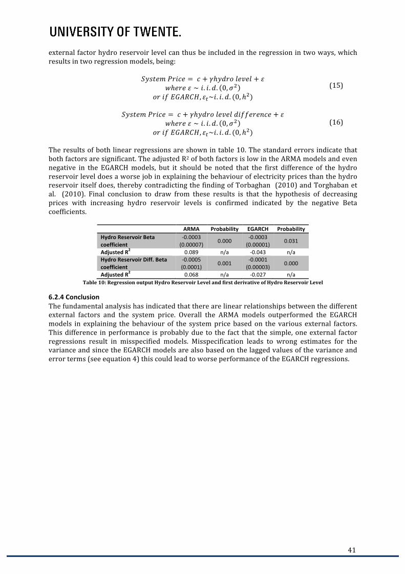
41
(15)
(16)
external factor hydro reservoir level can thus be included in the regression in two ways, which results in two regression models, being:
𝑆𝑦𝑠𝑡𝑒𝑚 𝑃𝑟𝑖𝑐𝑒 = 𝑐 + 𝛾ℎ𝑦𝑑𝑟𝑜 𝑙𝑒𝑣𝑒𝑙 + 𝜀 𝑤ℎ𝑒𝑟𝑒 𝜀 ∼ 𝑖. 𝑖.𝑑. 0,𝜎!
𝑜𝑟 𝑖𝑓 𝐸𝐺𝐴𝑅𝐶𝐻, 𝜀!~𝑖. 𝑖.𝑑. (0, ℎ!)
𝑆𝑦𝑠𝑡𝑒𝑚 𝑃𝑟𝑖𝑐𝑒 = 𝑐 + 𝛾ℎ𝑦𝑑𝑟𝑜 𝑙𝑒𝑣𝑒𝑙 𝑑𝑖𝑓𝑓𝑒𝑟𝑒𝑛𝑐𝑒 + 𝜀 𝑤ℎ𝑒𝑟𝑒 𝜀 ∼ 𝑖. 𝑖.𝑑. 0,𝜎!
𝑜𝑟 𝑖𝑓 𝐸𝐺𝐴𝑅𝐶𝐻, 𝜀!~𝑖. 𝑖.𝑑. (0, ℎ!) The results of both linear regressions are shown in table 10. The standard errors indicate that both factors are significant. The adjusted R2 of both factors is low in the ARMA models and even negative in the EGARCH models, but it should be noted that the first difference of the hydro reservoir level does a worse job in explaining the behaviour of electricity prices than the hydro reservoir itself does, thereby contradicting the finding of Torbaghan (2010) and Torghaban et al. (2010). Final conclusion to draw from these results is that the hypothesis of decreasing prices with increasing hydro reservoir levels is confirmed indicated by the negative Beta coefficients.
ARMA Probability EGARCH Probability Hydro Reservoir Beta coefficient
-‐0.0003 (0.00007) 0.000 -‐0.0003
(0.00001) 0.031
Adjusted R2 0.089 n/a -‐0.043 n/a Hydro Reservoir Diff. Beta coefficient
-‐0.0005 (0.0001) 0.001 -‐0.0001
(0.00003) 0.000
Adjusted R2 0.068 n/a -‐0.027 n/a Table 10: Regression output Hydro Reservoir Level and first derivative of Hydro Reservoir Level
6.2.4 Conclusion The fundamental analysis has indicated that there are linear relationships between the different external factors and the system price. Overall the ARMA models outperformed the EGARCH models in explaining the behaviour of the system price based on the various external factors. This difference in performance is probably due to the fact that the simple, one external factor regressions result in misspecified models. Misspecification leads to wrong estimates for the variance and since the EGARCH models are also based on the lagged values of the variance and error terms (see equation 4) this could lead to worse performance of the EGARCH regressions.


43
Chapter 7 – Framework Application The aim of this chapter is to utilise the knowledge gained in the previous chapter to construct forecasting models. Three forecasting models are developed, i.e. a technical model, a fundamental model and a merged model. The development of these models is presented in this chapter and it is determined which model provides the best forecast over a known period of time and therefore should be used to perform the out-‐of-‐data forecast in chapter 8.
7.1 Approach To construct the forecasting models it is necessary to align the data and to present evaluation measures that can measure the forecasting performance of the different models. This is further discussed below.
Data Evaluation To determine the performance of the forecasting models it is necessary to compare the forecasted values of the models with actual values. Therefore, the data should be split into a so-‐called training period and a forecasting period. The training period is used to estimate the models while the forecasting period is used for testing the forecasting ability of the models. There are two limitations to the forecasting period. First, the period cannot be too long (e.g. 10 years), since then the training period would be too short to estimate the model and approach the behaviour of the system price correctly. Secondly, the forecasting period should not be too short since it then would become irrelevant for project financing, dealing with long-‐term financing (i.e. 10-‐20 years). To cope with both limitations, the training period is set to 2000-‐2007 (8 years) and the forecasting period to 2008-‐2012 (5 years). A training period of 8 years is regarded to be sufficient to capture the behaviour of the system price while a forecasting period of 5 years gives a bit of an insight in the performance of the models and is regarded as long-‐term forecasting as mentioned in the literature review (chapter 4). Due to the limitations of the fundamental dataset, there is a difference between the periods used in the technical and the fundamental forecast models. The technical forecast model will use the data from January 2000 till December 2007 for the training period and the data from January 2008 till December 2012 for the forecasting period. Since 5 months of data are missing at the beginning of 2000 and 2 months of data at the end of 2012 for some external factors, the fundamental model will use the data from June 2000 till December 2007 for the training period and the data from January 2008 till October 2012 for the forecasting period. This means that the fundamental models will be based on fewer observations than the technical model, but since it is only a difference of 7 observations the impact should be limited.
Forecasting methods There are two different approaches that can be used to forecast the system price during the forecasting period, i.e. dynamic and static forecasting. Dynamic forecasting calculates dynamic, multi-‐step forecasts starting from the first period in the forecast sample. The values used for forming the forecasts are the previously forecasted values for the lagged dependent variable (i.e. the system price) (Eviews, 2010b). The choice to use dynamic forecasting is only available when an ARMA structure is present in the model. Therefore this can only be used for the technical models and the merged models, as will be discussed later on. The second method is static forecasting. Static forecasting calculates a sequence of one-‐step ahead forecasts using the actual values of the lagged dependent variable instead of the forecasted values. Static forecasts are more accurate than dynamic forecasts since they use the actual value in forming the forecast (Eviews, 2010b). In this research both methods will be applied. The static forecasting is more accurate, while the dynamic forecasting is more interesting for the purpose of this research. This is because the constructed model is used in chapter 8 to forecast the system price over a period of time in which there are no actual values known (out-‐of-‐data sample). Therefore it is relevant to

44
(17)
(18)
(19)
(20)
(21)
(22)
determine the performance of the different models under dynamic forecasting which calculates its forecasts on lagged forecasted dependent variables instead of actual values.
Forecast Evaluation All forecasting models constructed in this chapter are evaluated by several measures in order to compare their performance. The following measures have been chosen (Eviews, 2010b):
𝑀𝐴𝐸: 𝑦! − 𝑦!
!
!!!
/𝑛
𝑀𝐴𝑃𝐸: 100𝑦! − 𝑦!𝑦!
!
!!!
/𝑛
𝑇ℎ𝑒𝑖𝑙 𝐼𝑛𝑒𝑞𝑢𝑎𝑙𝑖𝑡𝑦 𝐶𝑜𝑒𝑓𝑓𝑖𝑐𝑖𝑒𝑛𝑡: (𝑦! − 𝑦!)!/𝑛!
!!!
𝑦!!/𝑛!!!! + 𝑦!!/𝑛!
!!!
𝐵𝑖𝑎𝑠 𝑃𝑟𝑜𝑝𝑜𝑟𝑡𝑖𝑜𝑛: ( 𝑦!!
!!!𝑛 − 𝑦)!
(𝑦! − 𝑦!)!/𝑛!!!!
Variance 𝑃𝑟𝑜𝑝𝑜𝑟𝑡𝑖𝑜𝑛: (𝑠! − 𝑠!)!
(𝑦! − 𝑦!)!/𝑛!!!!
Covariance 𝑃𝑟𝑜𝑝𝑜𝑟𝑡𝑖𝑜𝑛: 2(1 − 𝑟)𝑠!𝑠!(𝑦! − 𝑦!)!/𝑛!
!!!
MAE and MAPE stand for Mean Absolute Error and Mean Absolute Percentage Error respectively and are used as relative measures to compare forecasts for the same series across different models. The smaller the error, the better the ability of the model to forecast. The disadvantage of both measures is that they do not have an upper limit, which can be a problem due to the high volatility of electricity prices (Palmgren, 2008). To overcome this problem the Theil Inequality Coefficient is calculated. This value always lies between zero and one, where zero indicates a perfect fit. The bias, variance and covariance proportions are derived from the mean squared forecast error. The bias proportion tells how far the mean of the forecasts is from the mean of the actual series. The variance proportion indicates how far the variation of the forecast is from the variation of the actual series. The covariance proportion finally measures the remaining unsystematic forecasting errors (Eviews, 2010b). If the forecast of a model is good, the bias and variance proportions should be small so that most of the bias should be concentrated on the covariance proportion, because the three proportions always add up to one.
7.2 Technical Forecast Models In the technical analysis it was shown that the prices are subject to yearly seasonality, that prices are mean-‐reverting and that they have quite a high volatility. These characteristics of the system price will be taken into account in constructing technical forecast models.
7.2.1 Models presentation As mentioned in chapter 5 this research will use a two-‐step approach in constructing the forecasting models. The first step is to identify and select the right model based on an analysis similar to the technical analysis in chapter 6. The only difference is that the data now runs till

45
(23)
(24)
December 2007 instead of the end of 2012 due to the split in the training period and the forecasting period described in paragraph 7.1. The second step is to estimate the model.
Models identification and selection For the Box-‐Jenkins methodology to be valid, it is necessary that the time series to be analysed is mean-‐reverting (Enders, 1994). Since the data used to identify and estimate the models now ranges from 2000 till 2007, once again a unit-‐root test has to be applied to the dataset in the form of an augmented Dickey-‐Fuller test. The results of the test indicate that the null hypothesis of not mean-‐reverting is rejected as can be seen in Appendix H. This means that is it still valid to use the Box-‐Jenkins methodology. Furthermore, it should be tested whether heteroscedastic characteristics are present. Again an auxiliary regression is used to perform the three residual diagnostic tests described in the technical analysis (paragraph 6.1). The ARCH LM test indicates that the null hypothesis of homoscedasticity cannot be rejected. However, the White test and Correlogram of Squared Residuals do not reject the null hypothesis of homoscedasticity and therefore the models should account for this (see Appendix I). In order to do so, different ARCH models and ARMA models with robust standard errors are tested. The added value of these latter models is that they are easier to understand and to apply, which will enhance its application. Of the different ARCH models, the EGARCH specification was chosen since it performed the best over two separate testing periods (see Appendix J). Following the Box-‐Jenkins methodology it is valid to develop a model with AR and MA processes for the system price, hence the correlogram of the system price is examined. The correlogram contains information on the autocorrelation and partial correlation and is needed to identify the ARMA processes (see Appendix K). To identify the best model the Akaike and Schwarz criteria are used. Models till AR(6) have been included in the analysis since the correlogram indicates potentially significant lags at that height. Based on the correlogram and the Akaike and Schwarz criteria in total 14 ARMA models and 15 EGARCH models have been specified, presented in Appendix L. The models with the lowest Akaike and Schwarz criteria are the AR(1,2) model and EGARCH(1,1) model with an AR(1,2) process both and intercept. The AR(1,2) model is specified by equation 23 and the EGARCH(1,1) model by equation 24:
𝑦! = 𝑐 + 𝛽!𝑦!!! + 𝛽!𝑦!!! + 𝜀! 𝑤ℎ𝑒𝑟𝑒 𝜀!~𝑖. 𝑖.𝑑. (0,𝜎!)
𝑦! = 𝑐 + 𝛽!𝑦!!! + 𝛽!𝑦!!! + 𝜀!
𝑤ℎ𝑒𝑟𝑒 𝜀!~𝑖. 𝑖.𝑑. (0, ℎ!)
𝑎𝑛𝑑 ℎ! 𝑖𝑠 𝑑𝑒𝑟𝑖𝑣𝑒𝑑 𝑏𝑦: log 𝜎!! = 𝜔 + 𝜑! log 𝜎!!!! + 𝜃!𝜀!!!𝜎!!!
+ 𝜗!𝜀!!!𝜎!!!
Where C is an intercept, Yt is the system price, Yt-‐1 is the AR(1) process, Yt-‐2 is the AR(2) process, εt is the error term and the β’s are the coefficients of the AR processes that are estimated in the next part. Note that the EGARCH model has an equation for the variance itself and that the estimated variance derived from this equation is denoted by h2.
Models estimation The parameters of the ARMA model are estimated using Ordinary Least Squares (OLS) and the parameters of the EGARCH model by the Maximum Likelihood function. The estimation outputs can be found in Appendix M. The adjusted R2 and Akaike and Schwarz criteria are provided in table 11.
ARMA EGARCH
Adjusted R2 0.81 0.80 Akaike criterion 6.34 5.92 Schwarz criterion 6.42 6.11 Table 11: Technical models estimation output

46
The adjusted R2 indicates that the models fit the data reasonably well but that there is also room for improvement. Based on the Akaike and Scwharz criterion the EGARCH model is preferred above the ARMA model, due to the lower values for these criteria. The moderate performance of the models could be caused by the limited amount of observations. Another cause could be model misspecification. Therefore several residual tests are conducted. First test is to check the correlogram of the residuals to see whether there is correlation between the residuals indicating model misspecification. Based on the correlogram of residuals, not one correlation is indicated as significant and therefore it is concluded that there is no correlation in the residuals for both models (see Appendix N). Second test for the residuals is to determine if they are normally distributed. In order to do so the histograms and Jarque-‐Bera tests are performed which can be found in Appendix O. The histograms and the Jarque-‐Bera tests indicate that the residuals are not normally distributed for the ARMA model, but are for the EGARCH model. Non-‐normality of the residuals leads to higher errors compared to normal distributed residuals (as discussed in chapter 6), leading to the fact that the ARMA model performs worse than the EGARCH model. To overcome this issue the data series can be transformed by taking the natural logarithm of the series or the difference of the natural logarithm but that would make the model specification and forecasting less intuitive while still not transforming the residuals of the ARMA model into a normal distribution (see Appendix P).
7.2.2 Models forecast The identified and estimated technical models are applied in this paragraph to forecast the system price. As mentioned in paragraph 7.1, the aim is to forecast the system price during the testing period of January 2008 till December 2012. Both dynamic and static forecast methods have been used to determine the forecasting performance of the technical models. The results are presented in table 12 including the forecast evaluation measures described in paragraph 7.1.
Mean Abs. Error Perc.
Mean abs. Error
Theil Inequality
Bias Proportion
Variance Proportion
Covariance Proportion
ARMA Dynamic 27.988 13.096 0.230 0.406 0.383 0.211 ARMA Static 17.599 6.953 0.105 0.050 0.004 0.946 EGARCH Dynamic 30.048 14.187 0.250 0.464 0.277 0.259 EGARCH Static 16.147 6.432 0.099 0.049 0.016 0.935
Table 12: Forecast Evaluation of technical forecasting models As expected the dynamic forecasts perform worse than the static forecasts for both models. This is indicated by a higher MAPE, MAE and Theil Inequality. Also note that the bias, variance and covariance proportions ad up to one and that the static forecasts errors are mainly due to the covariance proportion, thereby indicating that they are better forecasts than the dynamic forecasts. The bias proportion for the dynamic forecasts reveals that the mean of the forecast series is far from the mean of the actual system price. This is overcome by the static forecast by using the actual values for the lagged dependent variable used in the forecast. Also note that the EGARCH model performs better in static forecasting but worse in dynamic forecasting compared to the ARMA model. This is probably because the EGARCH incorporates more lagged independent variables (i.e. in the variance equation).
7.3 Fundamental Forecast Models In the fundamental analysis hypotheses have been identified for various external factors on how they might impact the system price. It was concluded that all factors on its own did not have a strong linear relationship with the system price. In this part the research will analyse the combined effect of multiple fundamental factors on the electricity price and determine which combined fundamental factors can forecast the price the best.

47
(25)
(26)
7.3.1 Models presentation For the fundamental forecasting models also the two-‐step approach is used. The first step is to identify and select the right model based on analysis of the different regressions. The second step is to estimate the model and to analyse the model’s performance in fitting the historical behaviour of the electricity price.
Models identification and selection The selection of the best fundamental model is done in several steps. First, all external factors are included in the regression. The only limitation is that the factor hydro and the factor hydro_diff cannot be in the same regression since the latter is a derivative of the first. Even though the interconnectivity of the Nordic market is captured by as well the surrounding electricity markets as the interconnection in MWh, both factors can be included in the same regression. This is because it is believed there is no relevant correlation between the factors due to the fact that interconnection in MWh also includes other markets and that prices at the EEX and APX-‐ENDEX are also influenced by other factors than the Nord Pool system price. Based on a first regression, the second step is to examine the standard errors for each variable leading to the removal of external factors that are not indicated as significant. This is done as long as there are non-‐significant factors and as long as by removing them the adjusted R2 increases. The Beta coefficients of the variables are also examined to see whether they confirm the hypotheses, although this does not lead to the removal of significant factors when their Beta coefficient does not correspond to the specific hypothesis. This approach has led to two fundamental forecasting models (ARMA: equation 25; EGARCH: equation 26):
𝑦! = 𝛽!𝐺𝑎𝑠 + 𝛽!𝑂𝑖𝑙 + 𝛽!𝐷𝑒𝑚𝑎𝑛𝑑 + 𝛽!𝐼𝑛𝑡𝑒𝑟𝑐𝑜𝑛𝑛𝑒𝑐𝑡𝑖𝑜𝑛 + 𝛽!𝐶𝑜𝑎𝑙 + 𝜀! 𝑤ℎ𝑒𝑟𝑒 𝜀 ∼ 𝑖. 𝑖.𝑑. 0,𝜎!
𝑦! = 𝛽!𝐺𝑎𝑠 + 𝛽!𝑂𝑖𝑙 + 𝛽!𝐷𝑒𝑚𝑎𝑛𝑑 + 𝛽!𝐼𝑛𝑡𝑒𝑟𝑐𝑜𝑛𝑛𝑒𝑐𝑡𝑖𝑜𝑛 + 𝛽!𝐸𝐸𝑋 + 𝜀!
𝑤ℎ𝑒𝑟𝑒 𝜀!~𝑖. 𝑖.𝑑. (0, ℎ!)
𝑎𝑛𝑑 ℎ! 𝑖𝑠 𝑑𝑒𝑟𝑖𝑣𝑒𝑑 𝑏𝑦: log 𝜎!! = 𝜔 + 𝜑! log 𝜎!!!! + 𝜃!𝜀!!!𝜎!!!
+ 𝜗!𝜀!!!𝜎!!!
Both models incorporate the factors gas, oil, demand and interconnection. The difference is that the first incorporates coal, while the second incorporates the factor EEX. Note that, while it is believed that the level of hydro reservoirs impacts the system price, both fundamental models do not incorporate this external factor since both factors turned out to be non-‐significant in the regressions.
Models estimation The estimation of the fundamental models is done similar to the technical analysis. Table 13 presents the Beta coefficients of each external factor for both models and includes the adjusted R2 and Akaike and Schwarz criteria. The Beta coefficients follow the same notation as in equations 25 and 26, i.e. β1 is the coefficient estimate of gas, β2 for the oil etc.
α β1 β2 β3 β4 β5 β6 Adj. R2 Akaike Scwharz
ARMA -‐ 0.1211 (0.0394)
0.5044 (0.0715)
0.2823 (0.0916)
0.0145 (0.0015)
-‐0.2202 (0.0804) -‐ 0.745 6.668 6.801
EGARCH -‐ 0.0692 (0.0195)
0.2987 (0.0437)
0.2161 (0.0356)
0.0092 (0.0004) -‐ 0.0624
(0.0229) 0.592 6.253 6.501
Table 13: Fundamental Models Estimation Output Note: All estimate coefficients are significant at a 5% significance level.
Notice that most of the signs of the Beta coefficients match the hypotheses stated in the fundamental analysis (paragraph 6.2.2). For instance, the Beta coefficients for demand are positive, thereby indicating that when the demand increases the electricity price will increase.

48
€ 10
€ 20
€ 30
€ 40
€ 50
€ 60
€ 70
€ 80
€ 90
jan-08 jul-08 jan-09 jul-09 jan-10 jul-10 jan-11 jul-11 jan-12 jul-12
Forecast performance Fundamental Model
EGARCH Fundamental Static System Price Graph 3: Forecast Fundamental Model and System Price during 2008-‐2012
Notice also that some Beta coefficients are very small (e.g. the interconnection). This is because the used figures for the interconnection factor are much higher than the electricity price itself. The Beta coefficient of coal is the opposite of what the hypothesis stated. Because removal of the coal factor decreases the adj. R2 of the ARMA model, it is decided to keep the coal factor included. Lastly, note that the ARMA model fits the data better than the EGARCH model, indicated by the higher adjusted R2, but that the EGARCH model is better specified indicated by the lower Akaike and Schwarz criteria. In both cases, the adjusted R2 has increased significantly compared to the fundamental analysis of each factor on its own but is lower than the technical analysis. Also the Akaike and Schwarz criteria are worse than the technical analysis.
7.3.2 Models forecast The estimated fundamental models will now be used to forecast the system price between January 2008 and October 2012. The evaluation measures introduced in paragraph 7.1 are used to determine the performance of the models. Only a static forecast is performed with the fundamental models, since they do not include lagged independent variables. The results are presented in table 14. Based on the covariance proportion, the ARMA model is preferred above the EGARCH model, indicating that the misfit of the forecast is a result of unsystematic errors, while the MAPE, MAE and Theil Inequality all prefer the EGARCH model.
Mean Abs. Error Perc.
Mean abs. Error
Theil Inequality
Bias Proportion
Variance Proportion
Covariance Proportion
ARMA 19.743 8.524 0.133 0.160 0.036 0.804 EGARCH 17.208 7.257 0.116 0.353 0.084 0.563
Table 14: Forecast Evaluation of Fundamental Forecast Models To provide more insight in the performance of the forecasts, graph 3 presents the forecast of the fundamental EGARCH model compared to the system price over the period January 2008 till October 2012. From the graph it can be concluded that the fundamental model performs significantly worse during the period July 2008 and April 2009. After this period, the fundamental model fits the system price much better. Exclusion of the period between July 2008 and April 2009 would improve the forecast. Even though the period should not be excluded. The system price does not behave different in this period compared to other periods and therefore the reason for the misfit in year 2008 is attributable to the fundamental model itself. To exclude the year 2008 therefore does not improve the knowledge about the forecasting performance of the fundamental model, but instead might lead to wrong conclusions about the forecasting performance of the fundamental model.

49
(27)
(28)
(29)
(30)
7.4 Merged Forecast models The merged forecasting models incorporate both the technical and fundamental aspects. The technical forecasting models have so far proven to be superior over the fundamental forecasting models. This paragraph will investigate the performance of merged forecasting models.
7.4.1 Models presentation Since the data of fundamental factors is slightly limited due to the missing values for the first five months in 2000 of the EEX, the dataset from June 2000 till December 2007 is used for the training period. When the EEX is however indicated as non-‐significant the dataset is extended to incorporate the first five months of 2000. The two-‐step approach will also be used for developing the merged models.
Models identification and selection The merged models are a combination of the ARMA structure of the technical models and the fundamental factors of the fundamental models. The appropriate ARMA structure is found by investigating the correlogram and as in the technical analysis AR(1,2) models are the preferred models. To include the fundamental factors several statistic indicators are used. First of all the standard error for each factor in the regressions is checked to determine if the variable is significant or not. When the factor is indicated as non-‐significant it is removed from the regression. The adjusted R2 is examined before and after the removal of the external factor. This process is repeated until there is no further increase in the adjusted R2. The Akaike and Schwarz criteria are also investigated to determine whether exclusion of each non-‐significant factor decreases the criteria (thereby increasing the performance of the models). Finally, when determining which factors to exclude also the Beta coefficients are investigated to see if they correspond to the hypotheses set up in the fundamental analysis. This approach has led to four merged forecasting models, being the ARMA models in equation 27 and 28, and the EGARCH models in equation 29 and 30:
𝑦! = 𝛼 + 𝛽!𝑦!!! + 𝛽!𝑦!!! + 𝛽!𝑂𝑖𝑙 + 𝛽!𝐼𝑛𝑡𝑒𝑟𝑐𝑜𝑛𝑛𝑒𝑐𝑡𝑖𝑜𝑛 + 𝜀! 𝑤ℎ𝑒𝑟𝑒 𝜀 ∼ 𝑖. 𝑖.𝑑. 0,𝜎!
𝑦! = 𝛽!𝑦!!! + 𝛽!𝑦!!! + 𝛽!𝑂𝑖𝑙 + 𝛽!𝐼𝑛𝑡𝑒𝑟𝑐𝑜𝑛𝑛𝑒𝑐𝑡𝑖𝑜𝑛 + 𝛽!𝐷𝑒𝑚𝑎𝑛𝑑 + 𝜀!
𝑤ℎ𝑒𝑟𝑒 𝜀 ∼ 𝑖. 𝑖.𝑑. 0,𝜎!
𝑦! = 𝛽!𝑦!!! + 𝛽!𝑦!!! + 𝛽!𝑂𝑖𝑙 + 𝛽!𝐼𝑛𝑡𝑒𝑟𝑐𝑜𝑛𝑛𝑒𝑐𝑡𝑖𝑜𝑛 + 𝛽!𝐻𝑦𝑑𝑟𝑜_𝑑𝑖𝑓𝑓 + 𝜀! 𝑤ℎ𝑒𝑟𝑒 𝜀 ∼ 𝑖. 𝑖.𝑑. 0, ℎ!
𝑦! = 𝛼 + 𝛽!𝑦!!! + 𝛽!𝑦!!! + 𝛽!𝑂𝑖𝑙 + 𝛽!𝐼𝑛𝑡𝑒𝑟𝑐𝑜𝑛𝑛𝑒𝑐𝑡𝑖𝑜𝑛 + 𝛽!𝐺𝑎𝑠 + 𝛽!𝐻𝑦𝑑𝑟𝑜 + 𝜀!
𝑤ℎ𝑒𝑟𝑒 𝜀 ∼ 𝑖. 𝑖.𝑑. 0, ℎ! All models incorporate oil and interconnection. The first ARMA model has an intercept, and this intercept is replaced by the demand factor in the second ARMA model. The EGARCH models incorporate hydro factors. The differences are explained by the lagged independent variables applicable in the EGARCH models. For both the ARMA and EGARCH model, models are included without an intercept, since the believe is that an extra external factor is preferred above an intercept, because it gives more insight in which factors influence the system price.
Models estimation Like the previous models, the merged forecasting models are estimated using Ordinary Least Squares and Maximum Likelihood. Compared to the fundamental models, the merged models have excluded the factors coal and EEX. This is due to the inclusion of the ARMA structure. The external factors that are consistently included in all the merged models are oil and interconnection. The results of the models estimation are depicted in table 15a. The Beta

50
coefficients correspond to the equations above, i.e. β1 is the estimate coefficient of the AR(1) process, β2 for the AR(2) process etc.
α β1 β2 β3 β4 β5 β6 β7 β8
ARMA 1 15.7606 (3.8703)
1.1790 (0.1479)
-‐0.4273 (0.1394)
0.2908 (0.0965)
0.0065 (0.0011) -‐ -‐ -‐ -‐
ARMA 2 -‐ 1.0918 (0.1278)
-‐0.3508 (0.1227)
0.3866 (0.0885)
0.0068 (0.0012)
0.3484 (0.0981) -‐ -‐ -‐
EGARCH 1 -‐ 1.1939 (0.1108)
-‐0.3137 (0.1098)
0.2353 (0.0438)
0.0042 (0.0005) -‐ -‐ -‐ -‐0.0001
(4.1E-‐05)
EGARCH 2 27.7640 (3.8641)
1.1636 (0.0852)
-‐0.3217 (0.0967)
0.1140 (0.0550)
0.0042 (0.0003) -‐ 0.0357
(0.0090) -‐0.0001 (3.3E-‐05) -‐
Table 15a: Merged Models Estimation Output Note: All estimate coefficients are significant at a 5% significance level.
Adj. R2 Akaike Scwharz ARMA 1 0.867 6.010 6.145 ARMA 2 0.865 6.030 6.166 EGARCH 1 0.853 5.491 5.763 EGARCH 2 0.853 5.387 5.685
Table 15b: Merged Models Estimation Output Evaluation Measures Notice from the results in table 15b that based on the Akaike and Schwarz criteria the merged models fit the data better than the fundamental and the technical models. Also the Adjusted R2 increased compared to the earlier models, indicating a better performance. Of the four merged models, the models with an intercept fit the data better than the models without an intercept. Despite this difference, all four models are included in the forecasting section to determine their forecasting performance. To check if the models are not misspecified the same tests as in the technical model analysis are conducted. The correlograms of the models indicate that there is no correlation between the residuals (Appendix Q). The homoscedastic null hypothesis of the ARCH LM tests is not rejected for all models (Appendix R). Based on these findings the models are not misspecified. However, the residuals of both ARMA models are not normally distributed, based on the histograms and Jarque-‐Bera tests (Appendix S). As mentioned in the technical model part this increases the errors of the model.
7.4.2 Models forecast The merged models are now used to forecast the system price. The dataset has slightly changed compared to the fundamental models. Since the EEX is not included in the merged forecasting models, the starting point of the training period can be set to January 2000. This change does not affect the ranking of the models based on the Akaike and Schwarz criteria, thus the models selected earlier remain the best models to forecast with. Because the forecasts are dependent on the lagged dependent variables both the dynamic and static forecast are applied. The results of the forecasts can be found in table 16.
Mean Abs. Error Perc.
Mean abs. Error
Theil Inequality
Bias Proportion
Variance Proportion
Covariance Proportion
ARMA 1 Dynamic 18.465 7.899 0.130 0.231 0.314 0.455 ARMA 1 Static 16.068 6.256 0.096 0.028 0.008 0.964 ARMA 2 Dynamic 18.218 7.189 0.116 0.100 0.230 0.670 ARMA 2 Static 15.214 5.810 0.092 0.012 0.016 0.971 EGARCH 1 Dynamic 24.777 8.655 0.126 0.031 0.070 0.899 EGARCH 1 Static 15.355 5.757 0.092 0.001 0.005 0.995 EGARCH 2 Dynamic 20.702 9.624 0.161 0.409 0.362 0.229 EGARCH 2 Static 15.077 5.988 0.092 0.032 0.005 0.963
Table 16: Forecast Evaluation of Merged Forecast Models

51
Also in these results the static models outperform the dynamic models. The main difference between the static and the dynamic models is that the errors in the static forecasts are mainly due to unsystematic forecasting errors while in the dynamic forecasting models they are due to a mismatch between the means and the variances of the forecasted series and the actual values of the system price. To visualise the difference in performance, the dynamic and static forecasts of ARMA model 2 are presented in graph 4 alongside the system price during the forecast period. What can be seen from the graph is that the static forecast is more volatile, following the system price, while the dynamic forecast is less volatile and therefore performing less.
The results in table 16 finally also indicate that the dynamic ARMA model 2 without an intercept and with three external factors, being oil, demand and interconnection, outperforms the other dynamic forecasts based on the MAPE, MAE and Theil Inequality Coefficient. Also the covariance proportion is quite significant, indicating a good forecast, although it is not as high as the value for the dynamic EGARCH model 1 and off course the static forecasts.
7.5 Conclusion The analysis and forecasting models have shown that static models in general are better performing than the dynamic forecasting models. In chapter 8 a dynamic forecast is developed for the upcoming 15 years. For choosing the best model to do so, only dynamic forecasting models are therefore applicable. An overview of the performance of the technical and merged dynamic forecasting models is provided in table 17. The fundamental forecasting models are only based on static forecasts so therefore do not comply with the dynamic criterion. However, they are included in table 17 so that they can be compared to the other models. Of the dynamic models it is concluded that the merged models outperform the technical models, especially the ARMA merged models. These models perform better or (almost) equal to the static fundamental forecast, but since the latter are based on actual values instead of forecasted values this comparison is not reasonable. It only indicates the robust performance of the merged ARMA models.
€ 10
€ 20
€ 30
€ 40
€ 50
€ 60
€ 70
€ 80
€ 90
jan-08 jul-08 jan-09 jul-09 jan-10 jul-10 jan-11 jul-11 jan-12 jul-12
Forecast Performance Merged Model
System Price ARMA Merged Model 2 Dynamic ARMA Merged Model 2 Static
Graph 4: Static and Dynamic Forecast of Merged Model and System Price during 2008-‐2012

52
(31)
Mean Abs. Error Perc.
Mean abs. Error
Theil Inequality
Bias Proportion
Variance Proportion
Covariance Proportion
MERGED MODELS ARMA 1 Dynamic 18.465 7.899 0.130 0.231 0.314 0.455 ARMA 2 Dynamic 18.218 7.189 0.116 0.100 0.230 0.670 EGARCH 1 Dynamic 24.777 8.655 0.126 0.031 0.070 0.899 EGARCH 2 Dynamic 20.702 9.624 0.161 0.409 0.362 0.229
FUNDAMENTAL MODELS ARMA Static 19.743 8.524 0.133 0.160 0.036 0.804 EGARCH Static 17.208 7.257 0.116 0.353 0.084 0.563
TECHNICAL MODELS ARMA Dynamic 27.988 13.096 0.230 0.406 0.383 0.211 EGARCH Dynamic 30.048 14.187 0.250 0.464 0.277 0.259
Table 17: Forecast Evaluation of Dynamic Merged Forecast Models Note: The best performing model is highlighted in blue (ARMA 2 Dynamic Model)
Choosing the best dynamic model is objective as well as subjective. Based on the lowest MAPE, MAE and Theil inequality coefficient the ARMA merged model 2 performs the best, while based on the covariance proportion the EGARCH merged model 1 is preferred. The ARMA merged model 2 is however favoured due to the following reasons:
- It has a significant covariance proportion, indicating a good forecast (objective); - The first 3 evaluation measures (MAPE, MAE and Theil) indicate the model as the best
performing model (objective); - The model is easier to understand and to implement in chapter 8 than the EGARCH
models, due to the lack of a separate equation for the variance in the error term (subjective).
So the model that is regarded as the best forecasting model based on the forecasting period January 2008 – October 2012 and that will be used in chapter 8 is denoted by the following equation:
𝑦! = 𝛽!𝑦!!! + 𝛽!𝑦!!! + 𝛽!𝑂𝑖𝑙 + 𝛽!𝐼𝑛𝑡𝑒𝑟𝑐𝑜𝑛𝑛𝑒𝑐𝑡𝑖𝑜𝑛 + 𝛽!𝐷𝑒𝑚𝑎𝑛𝑑 + 𝜀! 𝑤ℎ𝑒𝑟𝑒 𝜀 ∼ 𝑖. 𝑖.𝑑. 0,𝜎!

53
Chapter 8 – Project Financing Perspective In this chapter the best performing model of chapter 7 is used to perform a long-‐term (15 year) out-‐of-‐data system price forecast. Long-‐term forecasting is relevant for renewable energy project finance since the revenues over this period should be determined and forecasted. As mentioned in chapter 3, the electricity price contributes the main part of the revenues, while selling the tradable green certificates generates the other small part of the revenues. Forecasting over a long period is very difficult and is completely dependent on the inputs that are used in order to perform the forecast. Instead of performing one, fixed forecast, the approach taken in this research is to establish multiple forecasts based on several scenarios. These different scenarios represent realistic assumptions and indicate how the system price in the Nordic countries will develop based on different assumptions. The first paragraph will introduce the different scenarios while the second paragraph will develop the forecasts of the external factors. The forecasts of the external factors are needed to forecast the system price in the third paragraph. The final paragraph will finalise this chapter with a short conclusion.
8.1 Scenarios The scenarios developed in this paragraph should include feasible assumptions for the three external factors included in the forecasting model and should provide useful information on how the system price can develop in the upcoming years. These criteria lead to the development of four different scenarios: a high, medium, low and alternative scenario, denoted in table 18. The first scenario assumes an increase in the oil price, an increase in the net import of electricity of the Nordic countries and an increase in demand. Since all the external factors have a positive Beta coefficient, these so-‐called high assumptions will lead to a higher system price. This first scenario is called the high scenario. The same goes for the second and third scenario where respectively moderate and low assumptions will be used to determine the future system price. These scenarios are called the medium and low scenario respectively. The alternative 4th scenario assumes a medium oil price, a low / negative import of electricity and a medium development of demand in the Nordic countries over the upcoming years. This fourth scenario is added since the other three scenarios are not regarded to capture all realistic future developments. The oil assumption is considered to be conservative, as will be explained later on. The low interconnection assumption is based on an International Energy Agency report indicating that the Nordic countries will become a net exporter of electricity in the upcoming years (IEA, 2013). The moderate demand seems reasonable, since in industrialised nations the demand is expected to remain unchanged or decrease due to governmental incentives to increase efficiency and cut CO2 emissions (Brown, Bolte, Zunder, & Meibeyer, 2012). The development, forecast and values for the different external factors under the different scenarios of high, medium and low will be discussed in paragraph 8.2.
Scenario Oil Interconnection Demand High High High High Medium Medium Medium Medium Low Low Low Low Alternative Medium Low Medium
Table 18: Scenarios for System Price Forecasting
8.2 External Factors forecast Based on the historical behaviour of the external factors, high, medium and low forecasts are developed for the different factors. The assumptions made for these forecasts are subjective but are supported by literature and opinions of experts. The subjective assumptions can be changed to develop new and/or more realistic scenarios, but are suitable for this research since the goal is to develop indications of how the system price might develop in the future based on reasonable assumptions.

54
8.2.1 Oil The underlying value used for oil is the Brent Crude Oil index. The development of the Brent Cure Oil index is depicted in graph 5. It can be seen that the price is described by a random walk, since the price follows random steps and does not have a mean or a clear trend. In other words, it is impossible to determine the future value of the Brent Crude Oil index. A unit-‐root test confirms that the index is a random walk by not rejecting the null hypothesis of non-‐stationary time series (see Appendix T). A way of dealing with a random walk is to generate a simulation model based on historic data and construct a future random walk. But as the name states, a random walk is random indeed and each simulation will have different predicted values. Therefore, instead of random values this research assumes different stable prices for the different scenarios for the oil price, i.e. a high stable price for the high scenario and low / medium prices for the low / medium scenarios respectively. These fixed prices are completely subjective. The low and medium fixed prices are lower than the current price of oil and it is assumed that in the upcoming years the price will decrease with 10% annually until the fixed price is reached. This has led to the following future values of the Brent Crude index over the next 15 years:
2012m12 2013 -‐ X X -‐ 2027 High 83.82 80 80 Medium 83.82 83.82*0.9X 60 Low 83.82 83.82*0.9X 40
Table 19: Scenarios for Brent Crude Oil Index Forecasting (in Euros) The X in table 19 denotes the year where the fixed prices of €60 and €40 of respectively the medium and low scenario are hit. For the medium scenario this is the year 2016 and the low scenario 2020. Thereafter, the fixed price is assumed to remain stable over the upcoming years.
8.2.2 Interconnection The interconnection factor denotes the net import of electricity of the Nordic countries from non-‐Nordic countries (such as Russia, the Netherlands and Germany). A unit-‐root test indicates that the time series of this factor during 2000-‐2012 is stationary (see Appendix U) and the histogram and Jarque-‐Bera test indicates that the null hypothesis of a normal distribution cannot be rejected (see Appendix V). Therefore, the mean and standard deviation of the time series will be used to determine the different scenarios for the interconnection values in the future. As denoted in Appendix V, the mean of the series is 421 MWh and the standard deviation is 928 MWh. The mean will be
€ 0
€ 20
€ 40
€ 60
€ 80
€ 100
Brent Crude Index
Graph 5: Historical Prices Brent Crude Oil Index
Graph 6: Historical Values of Net Interconnection between Nordic and non-‐Nordic Countries
-2000
-1000
0
1000
2000
3000 Interconnection (in MWh)

55
(32)
(33)
used for the medium scenario and will be fixed over the forecasting period. For the low scenario, the mean minus twice the standard deviation is taken for the last year (2027) and for the high scenario the mean plus twice the standard deviation. This ensures that the ultimate values lie in the 95% confidence interval of the series of the interconnection values. The difference of both extreme values and the mean is divided by the total number of periods till December 2027 leading to a linear 11 MWh annual increase / 9 MWh annual decrease value for the high / low scenario. This is denoted by table 20:
Mean St. Dev 2012m12 2013 -‐ 2026 2027 High 421 927 268 421+(11*(X-‐2013)) 2277 Medium 421 927 268 421 421 Low 421 927 268 421-‐(9*(X-‐2013)) -‐1434
Table 20: Scenarios for Interconnection Forecasting (in MWh)
8.2.3 Demand As described in the Fundamental Analysis (paragraph 6.2) the historical demand shows a clear seasonal cycle. This research uses exponential smoothing which provides an easy way of determining the seasonal cycles and forecasting the future values of the demand in the Nordic countries. For exponential smoothing, this research makes use of the Holt-‐Winter – Additive method. This method is appropriate for series with a linear time trend and additive seasonal variation. Since a trend will be included in the forecast, i.e. to incorporate future decrease or increase of interconnection depending on the scenario used, this method is chosen. The smoothed series 𝑧! is given by (Eviews, 2010a):
𝑧!!! = 𝑎 + 𝑏𝑘 + 𝑐!!! Where a and b are the permanent component and trend respectively and c is the additive seasonal factor. More information about exponential smoothing and the recursions of the three coefficients can be found in Appendix W. The historic demand and the smoothed series over the period January 2000 – October 2012 is given in graph 7 below:
The smoothed series fits the historic data of demand very well and therefore seems appropriate to use in forecasting the future values of demand. Forecasts of the exponential smoothed series are computed by:
𝑧!!! = 𝑎 𝑡 + 𝑏 𝑡 𝑘 + 𝑐!!!!!"
20
25
30
35
40
45
2000 2001 2002 2003 2004 2005 2006 2007 2008 2009 2010 2011 2012
Demand (in TWh)
Exp. Smoothing Series Demand (in TWh) Graph 7: Historical Values of Electricity Demand in Nordic Countries

56
(34)
The forecasted smoothed series is used as the medium scenario for the demand. The high scenario is based on the same series but assumes a 2% annual growth. The low scenario does the opposite and incorporates a 2% annual decrease in demand. The total reduction in electricity demand is however limited. Based on a report of the Danish Energy Analyses (n.d.) ambitious energy saving targets in Nordic countries could lead to a maximum 10% reduction every 10 years from 2010 onwards. Since the forecast is over 15 years, this leads to a maximum reduction of 15%. Therefore, the low scenario assumes 2% annual reduction in electricity demand until the maximum reduction is achieved, i.e. in year 2019. Thereafter the mean of the demand will be stable and seasonable fluctuations will still be present. In comparison, a recent study only assumes a total reduction in electricity demand of 8% until 2050 in the Nordic region (Danish Energy Analyses, 2013). Instead of a table, the different scenarios are depicted in graph 8 since this is easier to understand. Note that the seasonal fluctuations are also impacted by the increase or decrease in the high and low scenarios.
8.3 Model application Now that insight in the future values of the external factors that impact the system price is gained, the system price during the same period of time can be forecasted. In order to do so, the best performing forecasting model of chapter 7 should be estimated based on the complete historic data. Because demand is one of the external factors in the model (lacking data of November and December in 2012), the data used to estimate the model is January 2000 till October 2012. The outcome of the estimation concludes that the AR(2) (denoted by 𝛽!𝑦!!! in equation 31) process is no longer significant (see Appendix X). By excluding the AR(2) process, the adj. R2 increases and the Akaike and Schwarz criteria decrease, thereby indicating that the new model fits the data better than the previous one. The exclusion is a bit controversial since it was determined in chapter 7 that the model with the AR(2) process performed the best in forecasting the system price. When the new model is used to forecast the system price during January 2008 till October 2012, the model performs even slightly better. However, the residual diagnostics of the estimation of this model during the period January 2000 – December 2007 indicate that there was still correlation in the residuals, hence this model was not chosen in the previous historic forecast. The new estimation and residual diagnostics do not indicate any correlation in the residuals and since the forecasting performance of the new model is proven to be better than the earlier suggested model, the research will use the following model in forecasting the system price during January 2013 till December 2027:
𝑦! = 𝛽!𝑦!!! + 𝛽!𝑂𝑖𝑙 + 𝛽!𝐼𝑛𝑡𝑒𝑟𝑐𝑜𝑛𝑛𝑒𝑐𝑡𝑖𝑜𝑛 + 𝛽!𝐷𝑒𝑚𝑎𝑛𝑑 + 𝜀! 𝑤ℎ𝑒𝑟𝑒 𝜀 ∼ 𝑖. 𝑖.𝑑. 0,𝜎!
Note that this model is exactly the same as equation 31, which denotes the best performing forecasting model of chapter 7, except that the AR(2) process (denoted by 𝛽!𝑦!!! in equation 31) is excluded. In other words, based on the estimation of the model from 2000 till 2012, it is concluded that the system price of two months in the past no longer has a significant influence on the current system price. The external factors have remained the same.
15 20 25 30 35 40 45 50 55 60
2013
2014
2015
2016
2017
2018
2019
2020
2021
2022
2023
2024
2025
2026
2027
Demand (in TWh)
High Medium Low Graph 8: Forecast Scenarios Electricity Demand in Nordic Market

57
A problem for linear regression can be that the independent factors of the model have a high degree of correlation between each other. This problem is referred to as multi-‐collinearity and can distort the model estimation procedure (Alexander, 2001). To check if the forecasting model depicted in equation 34 is subject to multi-‐collinearity, the intercorrelations between the independent factors is determined and the Variance Inflation Factors are calculated (see Appendix Y). Both checks indicate that the model does not suffer from multi-‐collinearity. Now that the model is calibrated and forecasts of the external factors under different scenarios are provided, forecasts can be made for the system price in the upcoming 15 years. All four scenarios are forecasted and depicted in graph 9. The dashed lines in each forecast are the trend lines for each specific forecast:
The different scenarios show predictable behaviour. The system price in the low scenario drops during the forecast reaching a low value near €18,-‐ per MWh. The medium scenario stays flat (except for the seasonal fluctuations) and has a mean near the €40,-‐ per MWh. The high scenario increases significantly and reaches values near the €65,-‐ per MWh. Finally, the alternative scenario is a bit below the medium scenario. This is mainly due to the low assumption this scenario has for the interconnection, indicating that the Nordic countries will have a net export of electricity in the future. The alternative scenario is regarded as the most likely scenario while still being conservative. This because of the following reasons: 1) The medium oil assumption is regarded as quite low, since it is generally believed that oil prices will go up in the future due to increased scarcity of this fuel source; 2) Because in the past 12 years there is no trend in the electricity demand, the medium assumption (also lacking a trend) for the future demand seems to be the most likely; 3) The low assumption in the alternative scenario for interconnection is supported by the International Energy Agency as mentioned in paragraph 8.1, indicating that the Nordic market will be a net exporter of electricity in the future; 4) Furthermore, the correlations between these three external factors indicate that there is a negative correlation between oil and interconnection (Appendix Y). In other words, when oil prices go up, the interconnection value would go down. This is also the case in the alternative scenario where the oil assumption is higher (i.e. medium) than the interconnection assumption (i.e. low).
€ 0
€ 10
€ 20
€ 30
€ 40
€ 50
€ 60
€ 70
€ 80
2013 2014 2015 2016 2017 2018 2019 2020 2021 2022 2023 2024 2025 2026 2027
System Price Forecasts 2013-2027
High Medium Low Alternative Poly. (Alternative) Graph 9: 4 Scenario Forecasts of the System Price during 2013-‐2027
Note: Prices are not indexed by inflation

58
8.4 Conclusion The best performing model of chapter 7 is utilised in this chapter to forecast the system price over a period of 15 years in the future. Four different scenarios for future values of the underlying key factors, being demand, oil and interconnection, are introduced and the analysis of the key factors led to assumptions for the future values of these key factors. Based on these scenarios and assumptions, the future system price is determined. The high scenario indicates that the system price might increase steadily over the next 15 years to a level of circa €65,-‐ per MWh. The three other scenarios (i.e. medium, alternative and low) however show a stable or declining trend for the future system price. The alternative is regarded as being the most likely scenario with a declining trend over the next 15 years to a level of circa €27,-‐ per MWh in 2027. All in all, the model is able to predict future system prices based on reasonable assumptions forming a suitable and useable alternative.

59
Chapter 9 – Conclusion, Discussion & Recommendations The aim of this research was to develop an own view on the electricity prices in Norway and Sweden by analysing the behaviour of electricity prices. This is achieved by determining the key factors that influence the price and by forecasting the electricity price over a 15-‐year period. The conclusions of the analysis and forecast are presented separately in the first paragraph of this chapter. The second paragraph provides a discussion about the limitations and use of this research. Final recommendations can be found in the third paragraph.
9.1 Conclusions The analysis of the electricity prices in Norway and Sweden was based on the system price of the Nord Pool market exchange and on the whole Nordic market. The conclusions in this paragraph are thus only applicable for the system price. The goal of this research was separated in chapter 3 in two separate goals:
1. Analyse the key factors in Norway and Sweden that determine the electricity price behaviour;
2. Forecast the electricity price in Norway and Sweden for a long-‐term period in the future. The conclusions of this research are divided based on these two goals. Part 9.1.1 presents the conclusions with regard to the goal of analysing the behaviour and determining the key factors influencing the electricity price. Part 9.1.2 provides conclusions based on the 15-‐year system price forecast.
9.1.1 Analysis The technical analysis led to the conclusion that the system price is not a random walk. Instead, based on the conducted unit-‐root tests, the hypothesis of non-‐mean-‐reverting is rejected. This means that when the electricity price is below the mean it has a tendency to revert back to its mean (thus increase) and vice versa when the price is above its mean. Further research needs to be conducted to determine the mean of the price and to discover if there is a trend or not. The fundamental analysis indicated that only a few factors have a significant impact on the electricity price. The key factors that have a significant impact on the current monthly electricity price are oil, interconnection, demand and the electricity price of one month and two months in the past. Hydro reservoir levels do not have a significant impact on the electricity price. Reasons for this could be that the impact of hydro levels is captured by the other external factors. For instance, hydropower is part of the supply side of electricity, which is partly captured by interconnection. Furthermore, it is believed that supply of electricity is not price elastic but demand elastic. In other words, the supply of electricity depends on the demand, since generators will only produce when offtakers want to buy the electricity. In contrast, the supply of electricity does not depend on the price of electricity, because generators will not produce electricity when there is no demand even if the prices are high, because they are unable to sell the electricity. A final reason for hydro levels not having a significant impact on the system price can be found in the role of the thermal power plants in the Nordic market. As mentioned in paragraph 2.2.2, the thermal power plants act as swing production facilities, meaning that this capacity is used to balance the total production during the seasons when the level of hydropower generation in Norway and Sweden is low. Since oil is regarded as having a significant impact on the system price and is one of the fuels used for the CHP plants, this factor might indicate the indirect impact hydro levels have on the system price. Furthermore, instead of having a significant impact on the electricity price, it is expected that the hydro reservoir levels and generation might have a bigger impact on the certificates price. However, this is outside the scope of the research. A final conclusion from the analysis is that interconnection has a positive impact on the electricity price. That is, when the net import is positive, the price will go up and vice versa. The reason for this is that the Nordic market will only export more electricity than it imports when
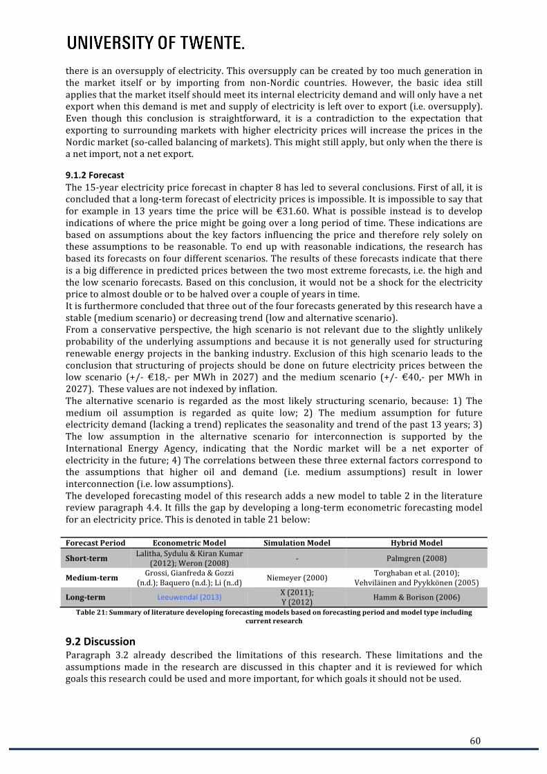
60
there is an oversupply of electricity. This oversupply can be created by too much generation in the market itself or by importing from non-‐Nordic countries. However, the basic idea still applies that the market itself should meet its internal electricity demand and will only have a net export when this demand is met and supply of electricity is left over to export (i.e. oversupply). Even though this conclusion is straightforward, it is a contradiction to the expectation that exporting to surrounding markets with higher electricity prices will increase the prices in the Nordic market (so-‐called balancing of markets). This might still apply, but only when the there is a net import, not a net export.
9.1.2 Forecast The 15-‐year electricity price forecast in chapter 8 has led to several conclusions. First of all, it is concluded that a long-‐term forecast of electricity prices is impossible. It is impossible to say that for example in 13 years time the price will be €31.60. What is possible instead is to develop indications of where the price might be going over a long period of time. These indications are based on assumptions about the key factors influencing the price and therefore rely solely on these assumptions to be reasonable. To end up with reasonable indications, the research has based its forecasts on four different scenarios. The results of these forecasts indicate that there is a big difference in predicted prices between the two most extreme forecasts, i.e. the high and the low scenario forecasts. Based on this conclusion, it would not be a shock for the electricity price to almost double or to be halved over a couple of years in time. It is furthermore concluded that three out of the four forecasts generated by this research have a stable (medium scenario) or decreasing trend (low and alternative scenario). From a conservative perspective, the high scenario is not relevant due to the slightly unlikely probability of the underlying assumptions and because it is not generally used for structuring renewable energy projects in the banking industry. Exclusion of this high scenario leads to the conclusion that structuring of projects should be done on future electricity prices between the low scenario (+/-‐ €18,-‐ per MWh in 2027) and the medium scenario (+/-‐ €40,-‐ per MWh in 2027). These values are not indexed by inflation. The alternative scenario is regarded as the most likely structuring scenario, because: 1) The medium oil assumption is regarded as quite low; 2) The medium assumption for future electricity demand (lacking a trend) replicates the seasonality and trend of the past 13 years; 3) The low assumption in the alternative scenario for interconnection is supported by the International Energy Agency, indicating that the Nordic market will be a net exporter of electricity in the future; 4) The correlations between these three external factors correspond to the assumptions that higher oil and demand (i.e. medium assumptions) result in lower interconnection (i.e. low assumptions). The developed forecasting model of this research adds a new model to table 2 in the literature review paragraph 4.4. It fills the gap by developing a long-‐term econometric forecasting model for an electricity price. This is denoted in table 21 below: Forecast Period Econometric Model Simulation Model Hybrid Model
Short-‐term Lalitha, Sydulu & Kiran Kumar (2012); Weron (2008) -‐ Palmgren (2008)
Medium-‐term Grossi, Gianfreda & Gozzi (n.d.); Baquero (n.d.); Li (n..d) Niemeyer (2000) Torghaban et al. (2010);
Vehviläinen and Pyykkönen (2005)
Long-‐term Leeuwendal (2013) X (2011); Y (2012) Hamm & Borison (2006)
Table 21: Summary of literature developing forecasting models based on forecasting period and model type including current research
9.2 Discussion Paragraph 3.2 already described the limitations of this research. These limitations and the assumptions made in the research are discussed in this chapter and it is reviewed for which goals this research could be used and more important, for which goals it should not be used.

61
Since the research only focuses on the system price, the conclusions about key factors influencing the electricity price only hold for the system price. The analysis and model of this research can thus not be used to forecast area prices. Instead of focussing on the system price, the research could instead have differentiated between the different areas prices in Norway and Sweden. Analyses based on these different area prices might lead to other conclusions and forecasting models due to e.g. country specific generation capacity. Specific analyses and forecasts for electricity prices in certain areas could be valuable assets when project finance opportunities arise in these areas. However, the focus on the system price was preferred because the system price forms the basis for the area prices and is thus a reasonable indicator for the area prices. Furthermore, since it is uncertain where future business opportunities might arise, all area prices should have been analysed and forecasted, potentially leading to multiple forecasting models. The focus on the system price limits the analysis to one price and results into one forecasting model, making the conclusions, forecasting model and recommendations easier to implement. The limited availability of historical values of the area prices, the unified Nordic electricity market and single exchange market (Nord Pool) further support the choice of analysing and forecasting the general system price instead of all area prices. As discussed in chapter 3 only (sort of) predictable, understandable factors are included in this research. This leads to the exclusion of factors that might have an impact on the electricity prices in the future. For instance, technology development: it might be the case that nuclear energy is dismantled in the Nordic market over the next 10 years and replaced by more expensive generation sources. Even though the marginal costs do not have a significant impact on the electricity price based on this research, a change in marginal cost due to this change in generation capacity might result in marginal costs having a significant impact on prices. Including less understandable and/or predictable factors in the analysis and forecast of the system price might improve the knowledge about the market and the electricity price. However, more research is needed to analyse which other factors influence the system price and how these factors behave and will behave. Recommendation 4 denotes this suggestion in paragraph 9.3. Even though that this suggestion might improve the forecasting model, reason for not including these unpredictable factors was that the goal of this research was to develop a transparent model that is easy to implement. The assumptions for the 15-‐year forecasts in chapter 8 are deliberately simple. The dynamics of the external factors are simplified. For instance, the oil and interconnection assumptions are in reality much more volatile than the linear assumptions included in the forecast. More insight in the underlying key factors and their behaviour will improve the knowledge about the electricity prices in Norway and Sweden and the reliability of the future prices calculated by the forecasting model. The simple assumptions are a limitation of this research and further research is needed as suggested in paragraph 9.3. The assumptions in this research for the long-‐term forecasts are kept simple in order to develop understandable, indicative forecasts based on reasonable scenarios, to gain insight in which key factors influence the (future) system price. Also do the forecasts not include the potential effects of the future electricity price on the price itself. For instance, when the prices become too low, it could be the case that generators stop producing electricity because it is no longer economically viable to do so (see Germany during the summer shutting down coals plants due to the oversupply of solar energy). This might result in prices to go up again for instance by increased import of electricity. On the other hand, if prices rise significantly, counter measures in the form of extra demand reductions might occur, having a negative impact on the electricity price. Not including the potential effects of the future electricity price on the price itself is again a limitation of this research and is subject to the fact that the assumptions for the key factors are deliberately simple. More extensive analysis of these key factors might lead to knowledge about the impact of the future electricity price on the price itself. Since the forecast in this research only aims to be an indicator for future values of the system price and limited time was available for conducting this research, these more extensive analyses are left out. The models developed in this research are regarded as simple time-‐series models. Alternative models could be developed to forecast the system price, such as artificial neural network models

62
(ANN models) or models based on wavelet decomposition techniques. These models might provide better forecasting performance than the models developed in this research. The choice for developing the simple ARMA and EGARCH time-‐series models is however justified by the criteria that the model should be transparent and useful. Furthermore, the inclusion of external factors in ARMA and EGARCH models is relatively straightforward, facilitating the analyses and forecasts of the fundamental and merged models of this research. Final point of discussion is that the forecasting model developed in this research should not form the only base for future electricity prices for structuring renewable energy projects. The research and model follow a different approach than other market consultants and thereby provide a different view and insight on electricity prices. It does not replace other forecasts, but instead should be seen as complimentary information to make informed decisions.
9.3 Recommendations Based on the goal, conclusions and limitations of this research, multiple recommendations are suggested. The first two recommendations focus on further developing and using the developed system price forecasting model of this research. Recommendations 3 till 6 indicate ideas for further research. Recommendation 1: Use developed model to perform free new forecasts The merged model used in chapter 8 to forecast the system price under different scenarios should be used to get indications of where the system price will go in the future. The user of the model can develop their own scenarios with regard to the three underlying key factors (i.e. demand, oil and interconnection) to forecast the future system price. An advantage of using this model is that the model is transparent (i.e. it is easy to understand how the model works and what the impact of the underlying key factors is) and free to use. It should however be noted that this model is based on the training period between 2000 and 2012 and therefore should not be used to perform forecasts starting from a starting date later than a couple of years after 2013. This restriction limits the possibility that the developed model becomes inapplicable and that market changes have deteriorated the performance of the model significantly. Recommendation 2: Analyse underlying external factors The main goal of this second recommendation is to indicate that the forecasting model of this research could be enhanced when the underlying factors are analysed more thoroughly. The future behaviour of these prices / values determine the future system price significantly (see different scenarios and system price forecast in chapter 8). Therefore a deeper understanding of the behaviour of these external factors leads to a better understanding of the development of the future system price and therefore to a better forecast. Instead of using the simple deterministic models developed in chapter 8 of this research for the underlying external factors incorporated in the model (i.e. demand, oil and interconnection), the user could improve the model by developing more sophisticated and/or stochastic models for the external factors. Recommendation 3: Analyse the mean and trend of the system price As mentioned in paragraph 9.1, one of the conclusions of this research is that the system price is mean-‐reverting. This means that the price has a tendency to revert back to its mean. The mean of the system price is relevant for the user since it indicates the average electricity price over a long period of time in the past and thereby indicates what the mean might be in the future. This research however does not indicate what the value is of this mean and if the mean is subject to a trend or not. Further research should be conducted to analyse the mean and the trend of the system price. Such an analysis is useful in that it provides more knowledge about the market and the electricity price and thereby adds to the necessary information to make educated decisions in future financing opportunities.

63
Recommendation 4: Analyse future market development and excluded key factors The literature review (chapter 4) suggested that there might be other factors influencing the system price that are outside the scope of this research. Further research should be conducted to determine which other factors have a significant impact on the system price and based on this analysis, new forecasting models can be developed. Also more insight should be gained in the development of the Nordic market in the future. Although it is (nearly) impossible to predict market changes, it is possible to construct reasonable assumptions about e.g. future build-‐out of electricity generators (wind, hydro, nuclear, thermal power plants etc.), potential changes to the support system for renewable energy projects and about the impact of a trans-‐European Super Grid (as introduced in paragraph 6.2.3). Including other external factors that influence the system price and analysing the future development of the Nordic market might lead to different conclusions and other forecasting models than constructed in this research. Recommendation 5: Analyse and forecast tradable green certificate price Besides the electricity price renewable energy projects also generate revenue by selling the tradable green certificates (as described in chapter 2). To predict the future cash flows of the renewable energy projects, the behaviour of the price of these certificates should therefore also be analysed. Such an analysis can be used to develop a model able to forecast the price of these certificates. This adds to the knowledge about future revenues and thus cash flows of projects in Norway and Sweden, necessary to structure and finance these projects.
Recommendation 6: Analyse if inflation is applicable to electricity price or not Another topic to be analysed is whether the electricity price in general should be indexed by inflation over the future years of a renewable energy project or not. It is common practice in renewable energy project finance to do so, but there are some voices in the market stating that electricity prices are actually not subject to inflation. Indexing electricity prices with 2% on an annual basis accumulates to almost 35% of the revenues in 15 year of the lifetime of a project. Indexing electricity prices or not thus impacts the revenues of renewable energy projects significantly and research about the relation between inflation and electricity prices should be conducted.


65
References Aggarwal, S.K., Saini, L.M., & Kumar, A. (2009). Electricity price forecasting in deregulated
markets: A review and evaluation. International Journal of Electrical Power & Energy Systems, 31(1), 13-‐22.
Alexander, C. (2001). Market Models -‐ A Guide to Financial Data Analysis. Chichester, England: John Wiley & Sons Ltd.
Amundsen, E.S., & Bergman, L. (2006). Why has the Nordic electricity market worked so well? Utilities Policy, 14(3), 148-‐157.
Baquero, L.A. (n.d.). ANN modeling of electric energy spot prices. Bask, M., Liu, T., & Widerberg, A. (2007). The stability of electricity prices: estimation and
inference of the Lyapunov exponents. Physica A: Statistical Mechanics and its Applications, 376, 565-‐572.
Bask, M., & Widerberg, A. (2009). Market structure and the stability and volatility of electricity prices. Energy Economics, 31(2), 278-‐288.
Benini, M., Marracci, M., Pelacchi, P., & Venturini, A. (2002). Day-‐ahead market price volatility analysis in deregulated electricity markets. Paper presented at the Power engineering Society Summer Meeting IEEE 2002.
Bergman, L. (2003). European electricity market integration: the Nordic experiences. Paper presented at the Research Symposium European Electricity Markets, The Hague, The Netherlands.
Bloomberg. (2012). Historical Data of External Factors such as: Hydro Reservoir Level, EEX & APX-‐ENDEX Prices, Marginal Costs. Retrieved on December 20th, 2012, from a Bloomberg Terminal.
Bottazzi, G., Sapio, S., & Secchi, A. (2005). Some statistical investigations on the nature and dynamics of electricity prices. Physica A: Statistical Mechanics and its Applications, 355(1), 54-‐61.
Botterud, A., Bhattacharyya, A.K., & Ilic, M. (2002). Futures and spot prices -‐ an analysis of the Scandinavian electricity market. Paper presented at the Proceedings of the 34th Annual North American power Symposium (NAPS 2002), Tempa, USA.
Box, G., & Jenkins, G. (1970). Time series analysis: Forecasting and control. San Francisco: Holden-‐Day.
Brown, T., Bolte, M., Zunder, I., & Meibeyer, K. (2012). Industry Portfolio Report -‐ Energy May 2012. Industry Portfolio Report NordLB.
CFA. (2009). Book 1 -‐ Ethical and Professional Standards, Quantative Methods, and Economics. Chartered Financial Analyst Study Books, K. Schweser (Ed.)
Danish Energy Analyses. (2013). Nordic Energy Technology Perspectives: Pathways to a Carbon Neutral Energy Future: Danish Energy Analyses Institute.
Danish Energy Analyses. (n.d.). Nordic electricity supply and demand in a changing climate: Danish Energy Analyses Institute.
Duarte, A.F., Fidalgo, J.N., & Saraiva, J.T. (2009). Forecasting electricity prices in spot markets—One week horizon approach. Paper presented at the IEEE Bucharest PowerTech, 2009.
Eberlein, E., & Stahl, G. (2003). Both sides of the fence: a statistical and regulatory view of electricity risk. Energy and Power Risk Management, 8(6), 32-‐36.
Enders, W. (1994). Applied Econometric Time Series. New York: John Wiley & Sons, Inc. ENS. (2012). Danish Energy Agency. Retrieved on December 31st, 2012, from http://www.ens.dk Erzgräber, H., Strozzi, F., Zaldívar, J.M., Touchette, H., Gutiérrez, E., & Arrowsmith, D.K. (2008).
Time series analysis and long range correlations of Nordic spot electricity market data. Physica A: Statistical Mechanics and its Applications, 387(26), 6567-‐6574.
Eurostat. (2012). European Statistics. Retrieved on December 7th, 2012, from http://www.epp.eurostat.ec.europa.eu

66
Eviews. (2010a). Eviews 7 User's Guide 1. Quantative Micro Software, LLC. Retrieved from http://www.eviews.com on December 15th, 2012.
Eviews. (2010b). Eviews 7 User's Guide 2. Quantative Micro Software, LLC. Retrieved from http://www.eviews.com on December 14th, 2012.
Fabini, C. (2012). Price forecasts in the european natural gas markets. (Master Thesis), University of St. Gallen.
Falconett, I., & Nagasaka, K. (2010). Comparative analysis of support mechanisms for renewable energy technologies using probability distributions. Renewable Energy, 35(6), 1135-‐1144.
Gianfreda, A. (2010). Volatility and volume effects in European electricity spot markets. Economic Notes, 39(1‐2), 47-‐63.
Gordon, S. (2006). Supergrid to the rescue. Power Engineer, 20(5), 30-‐33. Granger, C.W.J., & Jeon, Y. (2007). Long-‐term forecasting and evaluation. International Journal of
Forecasting, 23(4), 539-‐551. Grossi, L., Gianfreda, A., & Gozzi, G. (n.d.). Realized volatility models for electricity markets. Hamm, G., & Borison, A. (2006). Forecasting long-‐run electricity prices. The Electricity Journal,
19(7), 47-‐57. IEA. (2013). Nordic energy technology perspectives -‐ Pathways to a carbon neutral energy future:
International Energy Agency. IHS. (2012). Coal Information & Insight: IHS McCloskey. Retrieved on December 31st, 2012, from
http://www.ihs.com Kaygusuz, K., & Kaygusuz, A. (2002). Renewable energy and sustainable development in Turkey.
Renewable Energy, 25(3), 431-‐453. Kildegaard, A. (2008). Green certificate markets, the risk of over-‐investment, and the role of long-‐
term contracts. Energy Policy, 36(9), 3413-‐3421. Knittel, C.R., & Roberts, M.R. (2005). An empirical examination of restructured electricity prices.
Energy Economics, 27(5), 791-‐817. Kozhan, R. (2010). Financial Economectrics. de Volkskrant. Retrieved from
http://www.devolkskrant.nl/studieboeken on December 5th, 2012. Lalitha, S.V.N.L., Sydulu, M., & Kiran Kumar, M. (2012). Different ANN models for short-‐term
electricity price forecasting. Energy and Power, 2(1), 1-‐9. Li, C. (n.d.). Modeling and forecasting monthly electricity price of Sweden with periodic
autoregressive models. (D-‐level thesis in Statistics), Dalarna University, Sweden. Li, Y., & Flynn, P.C. (2004). Deregulated power prices: comparison of volatility. Energy Policy,
32(14), 1591-‐1601. Makridakis, S., & Hibon, M. (1998). ARMA models and the Box–Jenkins methodology. Journal of
Forecasting, 16(3), 147-‐163. Menanteau, P., Finon, D., & Lamy, M.-‐L. (2003). Prices versus quantities: choosing policies for
promoting the development of renewable energy. Energy Policy, 31(8), 799-‐812. Niemeyer, V. (2000, 4-‐7 Jan. 2000). Forecasting long-‐term electric price volatility for valuation of
real power options. Paper presented at the Proceedings of the 33rd Annual Hawaii International Conference on System Sciences -‐ 2000.
Nord Pool Spot. (2012). Monthly Elspot Prices. Retrieved on December 7th, 2012, from http://www.nordpoolspot.com
NordREG. (2012). Nordic Market Report 2012 -‐ Development in the Nordic Electricity Market:
NordREG -‐ Nordic Energy Regulators. O’brien, R.M. (2007). A caution regarding rules of thumb for variance inflation factors. Quality &
Quantity, 41(5), 673-‐690.

67
Palmgren, B. (2008). Forecasting Nordic electricity prices -‐ Utilizing a technical and fundamental analysis to develop a framework for forecasting electricity prices in Denmark, Finland, Norway and Sweden. (Master Thesis), Aarhus University, Sweden.
Project Finance Magazine. (2012). Project Finance BenchBase. Retrieved on December 7th, 2012,
from http://www.projectfinancemagazine.com. Robinson, T., & Baniak, A. (2002). The volatility of prices in the English and Welsh electricity pool.
Applied Economics, 34(12), 1487-‐1495. SCB. (2012). Statistics Sweden. Retrieved on December 31st, 2012, from http://www.scb.se Simonsen, I. (2005). Volatility of power markets. Physica A: Statistical Mechanics and its
Applications, 355(1), 10-‐20. Simonsen, I., Weron, R., & Mo, B. (2004). Structure and stylized facts of a deregulated power
market. SSB. (2012). Statistics Norway. Retrieved on December 31st, 2012, from http://www.ssb.no STAT. (2012). Statistics Finland. Retrieved on December 14th, 2012, from http://www.stat.fi Sterman, J.D. (1988). A Skeptic's Guide To Computer Models. Strozzi, F., Gutiérrez, E., Noè, C., Rossi, T., Serati, M., & Zaldívar, J.M. (2008). Measuring volatility
in the Nordic spot electricity market using Recurrence Quantification Analysis. The European Physical Journal-‐Special Topics, 164(1), 105-‐115.
Swedish Goverment. (2006). Renewable Electricity with Green Certificates. Swedish Ministry Of Sustainable Development.
Tashpulatov, S.N. (2011). Estimating the Volatility of Electricity Prices: The Case of the England and Wales Wholesale Electricity Market: The Center for Economic Research and Graduate Education -‐ Economic Institute, Prague.
The Windpower. (2012). Wind Turbines and Wind Farms Database. Retrieved on December 7th, 2012, from http://www.thewindpower.net
Torbaghan, S.S. (2010). Data Driven Medium Term Electricity Price Forecasting in Ontario Electricity Market and Nord Pool. (Master Thesis), Chalmers University of Technology, Göteborg, Sweden.
Torghaban, S., Zareipour, H., & Le, T. (2010). Medium-‐term electricity market price forecasting: A data-‐driven approach. Paper presented at the 42nd North American Power Symposium 2010, Arlington, USA.
Unger, T., & Ahlgren, E.O. (2005). Impacts of a common green certificate market on electricity and CO2-‐emission markets in the Nordic countries. Energy Policy, 33(16), 2152-‐2163.
Vehviläinen, I., & Pyykkönen, T. (2005). Stochastic factor model for electricity spot price—the case of the Nordic market. Energy Economics, 27(2), 351-‐367.
Weron, R. (2008). Forecasting wholesale electricity prices: A review of time series models.
Financial markets: principles of modelling, forecasting and decision-‐making, 71-‐82. Weron, R., Simonsen, I., & Wilman, P. (2004). Modeling highly volatile and seasonal markets:
evidence from the Nord Pool electricity market. H. Takayasu (edn.), The Application of Econophysics, Springer, Tokyo, 182-‐191.
Wolak, F.A. (2000). Market Design and Price Behavior in Restructured Electricity Markets: An International Comparison. In A. Faruqui & K. Eakin (Eds.), Pricing in Competitive Electricity Markets (Vol. 36, pp. 127-‐152): Springer US.
Zareipour, H., Bhattacharya, K., & Cañizares, C.A. (2007). Electricity market price volatility: The case of Ontario. Energy Policy, 35(9), 4739-‐4748.


69
Appendices
List of Appendices
Appendix A – EGARCH Model Page 70 Appendix B – Jarque-‐Bera Test Page 71 Appendix C – Dickey-‐Fuller Test System Price 2000-‐2012 Page 72 Appendix D – Dickey-‐Fuller Test Log System Price 2000-‐2012 Page 73 Appendix E – Correlogram of Squared Residuals System Price 2000-‐2012 Page 74 Appendix F – ARCH LM Test System Price 2000-‐2007 Page 75 Appendix G – White Test System Price 2000-‐2012 Page 76 Appendix H – Dickey-‐Fuller Test System Price 2000-‐2007 Page 77 Appendix I – Heteroscedasticity Tests System Price 2000-‐2007 Page 78 Appendix J – Comparison ARCH Models Page 80 Appendix K – Correlogram of System Price 2000-‐2007 Page 81 Appendix L – Summary of ARMA and EGARCH Models Page 82 Appendix M – Estimation Output Technical Models Page 83 Appendix N – Correlogram of Residuals Technical Models 2000-‐2007 Page 84 Appendix O – Histogram of Residuals Technical Models 2000-‐2007 Page 85 Appendix P – Histogram of Residuals Technical Model Log Price 2000-‐2007 Page 86 Appendix Q – Correlogram of Residuals Merged Models 2000-‐2007 Page 87 Appendix R – ARCH LM Test Merged Models 2000-‐2007 Page 89 Appendix S – Histogram of Residuals Merged Models 2000-‐2007 Page 91 Appendix T – Dickey-‐Fuller Test Brent Crude Oil Index 2000-‐2012 Page 93 Appendix U – Dickey-‐Fuller Test Interconnection 2000-‐2012 Page 94 Appendix V – Histogram of Interconnection 2000-‐2012 Page 95 Appendix W – Exponential Smoothing Page 96 Appendix X – Estimation Output Merged Model with AR(2) Process 2000-‐2012 Page 97 Appendix Y – Multi-‐collinearity Page 98 Appendix Z – Forecasting Output ARMA Merged Model 2 Dynamic 2008-‐2012 Page 99

70
Appendix A – EGARCH Model The EGARCH model stands for Exponential GARCH model. It is one of the extensions of the basic GARCH model and allows for the signs of the residuals or shocks to have an effect on the conditional volatility. Therefore, it captures a stylized fact of financial volatility that bad news (negative shocks) tends to have a larger impact on the volatility than good news (positive shocks) (so-‐called leverage effect) (Eviews, 2010b). The specific conditional variance of an EGARCH model is given by the following equation:
log 𝜎!! = 𝜔 + 𝜑!log (𝜎!!!!!
!!!
) + 𝜃!
!
!!!
𝜀!!!𝜎!!!
+ 𝜗!𝜀!!!𝜎!!!
!
!!!
Where the first factor is a constant factor 𝜔; the second factor is summarizing the log values of the previous conditional variances from previous periods 𝑗 = 1 𝑡𝑖𝑙𝑙 𝑞 (where q depends on how many lags are included). The conditional variances are denoted by 𝜎𝒕!𝒋! ; the third factor summarizes the absolute values of the previous residuals of the regression divided by the previous conditional variances from the previous periods 𝑖 = 1 𝑡𝑖𝑙𝑙 𝑝 (where p depends on how many lags how many lags are included). The previous residuals are denoted by 𝜀!!! . The final factor summarizes the values of the previous residuals of the regression divided by the previous conditional variances from the previous periods 𝑘 = 1 𝑡𝑖𝑙𝑙 𝑟 (where r depends on how many lags are included). The 𝜑! , 𝜃! 𝑎𝑛𝑑 𝜗! for the second, third and fourth factor respectively are estimated by the regression. Note that the left-‐hand side of the equation is the log of the conditional variance, implying that the leverage effect is exponential. The EGARCH model used in this research only includes one lag of each factor described above. Therefore, the equation of the conditional variance simplifies to the equation below due to the fact that the sum functions disappear:
log 𝜎!! = 𝜔 + 𝜑! log 𝜎!!!! + 𝜃!𝜀!!!𝜎!!!
+ 𝜗!𝜀!!!𝜎!!!

71
Appendix B – Jarque-‐Bera Test The Jarque-‐Bera test is used for normality testing. It tests whether the sample data has a skewness and kurtosis similar to a normal distribution. The statistic is computed as follows:
Jarque − Bera = N6
S! +K − 3 !
4
where N is the number of observations, S is the sample skewness and K is the kurtosis. The reported probability is the probability that a Jarque-‐Bera statistic exceeds the observed value under the null hypothesis. A small probability value leads to the rejection of the null hypothesis of a normal distribution.
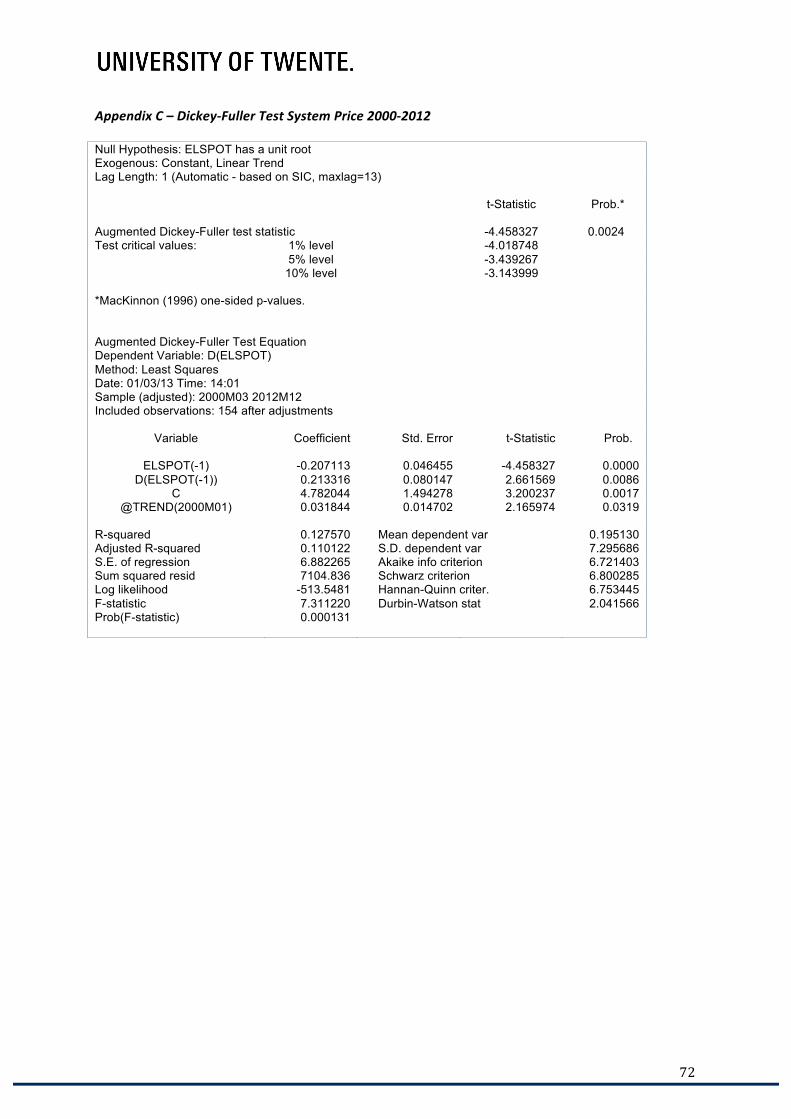
72
Appendix C – Dickey-‐Fuller Test System Price 2000-‐2012 Null Hypothesis: ELSPOT has a unit root Exogenous: Constant, Linear Trend Lag Length: 1 (Automatic - based on SIC, maxlag=13)
t-Statistic
Prob.*
Augmented Dickey-Fuller test statistic -4.458327 0.0024 Test critical values: 1% level -4.018748
5% level -3.439267
10% level
-3.143999
*MacKinnon (1996) one-sided p-values.
Augmented Dickey-Fuller Test Equation Dependent Variable: D(ELSPOT) Method: Least Squares Date: 01/03/13 Time: 14:01 Sample (adjusted): 2000M03 2012M12 Included observations: 154 after adjustments
Variable
Coefficient
Std. Error
t-Statistic
Prob.
ELSPOT(-1) -0.207113 0.046455 -4.458327 0.0000 D(ELSPOT(-1)) 0.213316 0.080147 2.661569 0.0086
C 4.782044 1.494278 3.200237 0.0017 @TREND(2000M01)
0.031844
0.014702
2.165974
0.0319
R-squared 0.127570 Mean dependent var 0.195130 Adjusted R-squared 0.110122 S.D. dependent var 7.295686 S.E. of regression 6.882265 Akaike info criterion 6.721403 Sum squared resid 7104.836 Schwarz criterion 6.800285 Log likelihood -513.5481 Hannan-Quinn criter. 6.753445 F-statistic 7.311220 Durbin-Watson stat 2.041566 Prob(F-statistic)
0.000131

73
Appendix D – Dickey-‐Fuller Test Log System Price 2000-‐2012 Null Hypothesis: LOG_ELSPOT has a unit root Exogenous: Constant, Linear Trend Lag Length: 0 (Automatic - based on SIC, maxlag=13)
t-Statistic
Prob.*
Augmented Dickey-Fuller test statistic -3.435549 0.0504 Test critical values: 1% level -4.018349
5% level -3.439075
10% level
-3.143887
*MacKinnon (1996) one-sided p-values.
Augmented Dickey-Fuller Test Equation Dependent Variable: D(LOG_ELSPOT) Method: Least Squares Date: 01/03/13 Time: 14:02 Sample (adjusted): 2000M02 2012M12 Included observations: 155 after adjustments
Variable
Coefficient
Std. Error
t-Statistic
Prob.
LOG_ELSPOT(-1) -0.143401 0.041740 -3.435549 0.0008 C 0.441614 0.128533 3.435792 0.0008
@TREND(2000M01)
0.000742
0.000418
1.772966
0.0782
R-squared 0.072402 Mean dependent var 0.006281 Adjusted R-squared 0.060196 S.D. dependent var 0.196653 S.E. of regression 0.190642 Akaike info criterion -0.457676 Sum squared resid 5.524334 Schwarz criterion -0.398771 Log likelihood 38.46987 Hannan-Quinn criter. -0.433750 F-statistic 5.932008 Durbin-Watson stat 1.787016 Prob(F-statistic)
0.003306

74
Appendix E – Correlogram of Squared Residuals System Price 2000-‐2012

75
Appendix F – ARCH LM Test System Price 2000-‐2012 Heteroskedasticity Test: ARCH
F-statistic 1.445728 Prob. F(1,151) 0.2311 Obs*R-squared
1.450985
Prob. Chi-Square(1)
0.2284
Test Equation: Dependent Variable: RESID^2 Method: Least Squares Date: 01/10/13 Time: 18:30 Sample (adjusted): 2000M04 2012M12 Included observations: 153 after adjustments
Variable
Coefficient
Std. Error
t-Statistic
Prob.
C 43.16996 10.05337 4.294077 0.0000 RESID^2(-1)
0.097377
0.080986
1.202384
0.2311
R-squared 0.009484 Mean dependent var 47.78578 Adjusted R-squared 0.002924 S.D. dependent var 115.0987 S.E. of regression 114.9304 Akaike info criterion 12.33952 Sum squared resid 1994557. Schwarz criterion 12.37913 Log likelihood -941.9729 Hannan-Quinn criter. 12.35561 F-statistic 1.445728 Durbin-Watson stat 2.018847 Prob(F-statistic)
0.231097

76
Appendix G – White Test System Price 2000-‐2012 Heteroskedasticity Test: White
F-statistic 3.307069 Prob. F(5,148) 0.0073 Obs*R-squared 15.47657 Prob. Chi-Square(5) 0.0085 Scaled explained SS
42.99554
Prob. Chi-Square(5)
0.0000
Test Equation: Dependent Variable: RESID^2 Method: Least Squares Date: 01/10/13 Time: 18:24 Sample: 2000M03 2012M12 Included observations: 154 Collinear test regressors dropped from specification
Variable
Coefficient
Std. Error
t-Statistic
Prob.
C 58.48572 12.20446 4.792160 0.0000 GRADF_01*GRADF_02 32.13983 10.71273 3.000154 0.0032 GRADF_01*GRADF_03 -18.08344 10.58969 -1.707647 0.0898
GRADF_02^2 -0.079905 0.088120 -0.906780 0.3660 GRADF_02*GRADF_03 0.122187 0.194274 0.628944 0.5304
GRADF_03^2
-0.068633
0.117146
-0.585879
0.5588
R-squared 0.100497 Mean dependent var 47.57824 Adjusted R-squared 0.070109 S.D. dependent var 114.7509 S.E. of regression 110.6553 Akaike info criterion 12.28890 Sum squared resid 1812200. Schwarz criterion 12.40722 Log likelihood -940.2452 Hannan-Quinn criter. 12.33696 F-statistic 3.307069 Durbin-Watson stat 2.036230 Prob(F-statistic)
0.007340

77
Appendix H – Dickey-‐Fuller Test System Price 2000-‐2007 Null Hypothesis: ELSPOT has a unit root Exogenous: Constant, Linear Trend Lag Length: 1 (Automatic - based on SIC, maxlag=11)
t-Statistic
Prob.*
Augmented Dickey-Fuller test statistic -4.221746 0.0061 Test critical values: 1% level -4.058619
5% level -3.458326
10% level
-3.155161
*MacKinnon (1996) one-sided p-values.
Augmented Dickey-Fuller Test Equation Dependent Variable: D(ELSPOT) Method: Least Squares Date: 01/03/13 Time: 17:31 Sample (adjusted): 2000M03 2007M12 Included observations: 94 after adjustments
Variable
Coefficient
Std. Error
t-Statistic
Prob.
ELSPOT(-1) -0.221789 0.052535 -4.221746 0.0001 D(ELSPOT(-1)) 0.438771 0.094616 4.637393 0.0000
C 4.287876 1.512695 2.834595 0.0057 @TREND(2000M01)
0.049736
0.024368
2.041048
0.0442
R-squared 0.254852 Mean dependent var 0.351915 Adjusted R-squared 0.230014 S.D. dependent var 6.362040 S.E. of regression 5.582619 Akaike info criterion 6.318814 Sum squared resid 2804.907 Schwarz criterion 6.427040 Log likelihood -292.9843 Hannan-Quinn criter. 6.362529 F-statistic 10.26045 Durbin-Watson stat 1.977213 Prob(F-statistic)
0.000007

78
Appendix I – Heteroscedasticity Tests System Price 2000-‐2007 ARCH LM Test: Heteroskedasticity Test: ARCH
F-statistic 1.385327 Prob. F(1,91) 0.2423 Obs*R-squared
1.394545
Prob. Chi-Square(1)
0.2376
Test Equation: Dependent Variable: RESID^2 Method: Least Squares Date: 01/15/13 Time: 11:20 Sample (adjusted): 2000M04 2007M12 Included observations: 93 after adjustments
Variable
Coefficient
Std. Error
t-Statistic
Prob.
C 27.61302 10.28661 2.684365 0.0086 RESID^2(-1)
0.122481
0.104062
1.176999
0.2423
R-squared 0.014995 Mean dependent var 31.47686 Adjusted R-squared 0.004171 S.D. dependent var 94.21001 S.E. of regression 94.01333 Akaike info criterion 11.94602 Sum squared resid 804304.1 Schwarz criterion 12.00049 Log likelihood -553.4900 Hannan-Quinn criter. 11.96801 F-statistic 1.385327 Durbin-Watson stat 2.059833 Prob(F-statistic)
0.242265
White Test: Heteroskedasticity Test: White
F-statistic 2.627647 Prob. F(5,88) 0.0291 Obs*R-squared 12.21095 Prob. Chi-Square(5) 0.0320 Scaled explained SS
51.02964
Prob. Chi-Square(5)
0.0000
Test Equation: Dependent Variable: RESID^2 Method: Least Squares Date: 01/15/13 Time: 11:20 Sample: 2000M03 2007M12 Included observations: 94 Collinear test regressors dropped from specification
Variable
Coefficient
Std. Error
t-Statistic
Prob.
C 31.32176 12.05907 2.597361 0.0110 GRADF_01*GRADF_02 36.75306 13.46501 2.729525 0.0077 GRADF_01*GRADF_03 -25.44303 13.46021 -1.890241 0.0620
GRADF_02^2 -0.085131 0.097050 -0.877192 0.3828 GRADF_02*GRADF_03 0.043348 0.200759 0.215923 0.8295
GRADF_03^2
0.053215
0.121713
0.437217
0.6630
R-squared 0.129904 Mean dependent var 31.22063 Adjusted R-squared 0.080466 S.D. dependent var 93.73506 S.E. of regression 89.88472 Akaike info criterion 11.89663 Sum squared resid 710975.1 Schwarz criterion 12.05897 Log likelihood -553.1418 Hannan-Quinn criter. 11.96221 F-statistic 2.627647 Durbin-Watson stat 2.068163 Prob(F-statistic)
0.029113

79
Correlogram of Squared Residuals System Price 2000-‐2007:

80
Appendix J – Comparison ARCH Models Four different ARCH models have been estimated during the periods 2000-‐2007 and 2000-‐2012. The regressions are analysed based on the correlation in the residuals, the hypothesis for the residuals to have a normal distribution and on the fit of the models with historical electricity prices based on the adjusted R2, Akaike and Schwarz criteria. Over the first period, the EGARCH model is preferred due to the highest adj. R2 (together with the PARCH model) and the lowest Akaike and Schwarz criteria (see table below). Period: 2000-‐2007 Correlation
Residuals Jarque-‐Bera Adj. R2 Akaike Schwarz
GARCH No 0.80 0.79 5.97 6.13 EGARCH No 0.68 0.80 5.92 6.11 PARCH No 0.76 0.80 5.92 6.13 C-‐GARCH No 0.00 0.80 6.03 6.25
Over the second period, the GARCH and C-‐GARCH models have correlations in their residuals and therefore are misspecified. The EGARCH model is preferred above the PARCH model due to its lower Akaike and Schwarz criteria and due to the observation that one factor in the volatility equation of the PARCH model is not significant with an alpha-‐level of 0.20. Period: 2000-‐2012 Correlation
Residuals Jarque-‐Bera Adj. R2 Akaike Schwarz
GARCH Yes 0.10 0.76 6.43 6.55 EGARCH No 0.11 0.76 6.38 6.51 PARCH No 0.27 0.76 6.37 6.53 C-‐GARCH Yes 0.07 0.76 6.39 6.54
Concluding, when an ARCH model is used, the research should use an EGARCH model.

81
Appendix K – Correlogram of System Price 2000-‐2007

82
Appendix L – Summary of all ARMA and EGARCH models
ARMA MODELS Model Intercept AR(p) MA(q) Adj.R2 Akaike Schwarz Model 1 C AR(1) AR(2) -‐ 0.81 6.34 6.42 Model 2 C AR(1) MA(1) 0.81 6.35 6.43 Model 3 C AR(1) AR(2) AR(5) -‐ 0.80 6.38 6.49 Model 4 C AR(1) AR(2) AR(5) AR(6) -‐ 0.79 6.40 6.54 Model 5 -‐ AR(1) MA(1) 0.80 6.42 6.47 Model 6 C AR(1) AR(2) AR(4) AR(5) AR(6) -‐ 0.79 6.42 6.59 Model 7 C AR(1) AR(2) AR(3) AR(4) AR(5) AR(6) -‐ 0.79 6.44 6.64 Model 8 -‐ AR(1) AR(2) -‐ 0.79 6.45 6.50 Model 9 -‐ AR(1) AR(2) AR(5) -‐ 0.78 6.45 6.53 Model 10 -‐ AR(1) AR(2) AR(3) AR(5) -‐ 0.78 6.47 6.58 Model 11 -‐ AR(1) AR(2) AR(3) AR(4) AR(5) -‐ 0.78 6.49 6.63 Model 12 C AR(1) -‐ 0.78 6.51 6.56 Model 13 -‐ AR(1) AR(2) AR(3) AR(4) AR(5) AR(6) -‐ 0.77 6.52 6.69 Model 14 -‐ AR(1) -‐ 0.77 6.54 6.57
EGARCH MODELS
Model Intercept AR(p) MA(q) Adj. R2 Akaike Schwarz Model 1 C AR(1) AR(2) -‐ 0.80 5.92 6.11 Model 2 C AR(1) MA(1) 0.79 5.93 6.12 Model 3 -‐ AR(1) MA(1) 0.79 5.96 6.12 Model 4 -‐ AR(1) AR(2) -‐ 0.78 5.96 6.12 Model 5 C AR(1) AR(2) AR(4) AR(5) -‐ 0.78 5.93 6.18 Model 6 C AR(1) AR(4) -‐ 0.77 5.92 6.11 Model 7 C AR(1) AR(2) AR(4) AR(5) AR(6) -‐ 0.77 5.95 6.23 Model 8 C AR(1) AR(4) AR(5) -‐ 0.77 5.91 6.13 Model 9 C AR(1) -‐ 0.76 5.95 6.09 Model 10 C AR(1) AR(2) AR(3) AR(4) AR(5) AR(6) -‐ 0.76 5.97 6.28 Model 11 -‐ AR(1) AR(2) AR(4) AR(5) AR(6) -‐ 0.76 6.07 6.32 Model 12 -‐ AR(1) AR(2) AR(4) AR(5) -‐ 0.75 6.03 6.25 Model 13 -‐ AR(1) AR(2) AR(3) AR(4) AR(5) AR(6) -‐ 0.75 6.09 6.37 Model 14 -‐ AR(1) AR(4) -‐ 0.75 6.01 6.17 Model 15 -‐ AR(1) AR(4) AR(5) -‐ 0.75 6.01 6.20

83
Appendix M – Estimation Output Technical Models ARMA Model: Dependent Variable: ELSPOT Method: Least Squares Date: 01/15/13 Time: 10:59 Sample (adjusted): 2000M03 2007M12 Included observations: 94 after adjustments Convergence achieved after 3 iterations White heteroskedasticity-consistent standard errors & covariance
Variable
Coefficient
Std. Error
t-Statistic
Prob.
C 30.55628 3.724039 8.205143 0.0000 AR(1) 1.244886 0.144657 8.605787 0.0000 AR(2)
-0.413978
0.135477
-3.055699
0.0029
R-squared 0.815305 Mean dependent var 29.59532 Adjusted R-squared 0.811246 S.D. dependent var 13.07120 S.E. of regression 5.678898 Akaike info criterion 6.342786 Sum squared resid 2934.739 Schwarz criterion 6.423955 Log likelihood -295.1109 Hannan-Quinn criter. 6.375572 F-statistic 200.8519 Durbin-Watson stat 1.947173 Prob(F-statistic)
0.000000
Inverted AR Roots
.62-.16i
.62+.16i
EGARCH Model: Dependent Variable: ELSPOT Method: ML - ARCH (Marquardt) - Normal distribution Date: 01/18/13 Time: 14:33 Sample (adjusted): 2000M03 2007M12 Included observations: 94 after adjustments Convergence achieved after 35 iterations Bollerslev-Wooldridge robust standard errors & covariance Presample variance: backcast (parameter = 0.7) LOG(GARCH) = C(4) + C(5)*ABS(RESID(-1)/@SQRT(GARCH(-1))) + C(6) *RESID(-1)/@SQRT(GARCH(-1)) + C(7)*LOG(GARCH(-1))
Variable
Coefficient
Std. Error
z-Statistic
Prob.
C 28.12984 3.076999 9.141971 0.0000 AR(1) 1.059560 0.094161 11.25259 0.0000 AR(2)
-0.193521
0.089765
-2.155862
0.0311
Variance Equation
C(4) 0.367875 0.246824 1.490436 0.1361 C(5) 0.531729 0.275946 1.926930 0.0540 C(6) 0.433890 0.156379 2.774610 0.0055 C(7)
0.734045
0.073755
9.952427
0.0000
R-squared 0.803264 Mean dependent var 29.59532 Adjusted R-squared 0.798940 S.D. dependent var 13.07120 S.E. of regression 5.861083 Akaike info criterion 5.920202 Sum squared resid 3126.058 Schwarz criterion 6.109596 Log likelihood -271.2495 Hannan-Quinn criter. 5.996703 Durbin-Watson stat
1.577065
Inverted AR Roots
.82
.23

84
Appendix N – Correlogram of Residuals Technical Models 2000-‐2007 ARMA Model: EGARCH Model:

85
Appendix O – Histogram of Residuals of System Price Regression 2000-‐2007 ARMA Model:
EGARCH Model:

86
Appendix P – Histogram of Residuals Technical Model Log System Price 2000-‐2007 ARMA Model:

87
Appendix Q – Correlogram of Residuals Merged Models 2000-‐2007 ARMA Model 1: ARMA Model 2:

88
EGARCH Model 1: EGARCH Model 2:

89
Appendix R – ARCH LM Test Merged Models 2000-‐2007 ARMA Model 1: Heteroskedasticity Test: ARCH
F-statistic 1.198252 Prob. F(1,91) 0.2766 Obs*R-squared
1.208672
Prob. Chi-Square(1)
0.2716
Test Equation: Dependent Variable: RESID^2 Method: Least Squares Date: 03/20/13 Time: 16:28 Sample (adjusted): 2000M04 2007M12 Included observations: 93 after adjustments
Variable
Coefficient
Std. Error
t-Statistic
Prob.
C 19.22583 7.766415 2.475509 0.0152 RESID^2(-1)
0.113954
0.104101
1.094647
0.2766
R-squared 0.012996 Mean dependent var 21.67930 Adjusted R-squared 0.002150 S.D. dependent var 71.78709 S.E. of regression 71.70986 Akaike info criterion 11.40440 Sum squared resid 467949.7 Schwarz criterion 11.45887 Log likelihood -528.3048 Hannan-Quinn criter. 11.42640 F-statistic 1.198252 Durbin-Watson stat 2.041544 Prob(F-statistic)
0.276560
ARMA Model 2: Heteroskedasticity Test: ARCH
F-statistic 0.733588 Prob. F(1,91) 0.3940 Obs*R-squared
0.743715
Prob. Chi-Square(1)
0.3885
Test Equation: Dependent Variable: RESID^2 Method: Least Squares Date: 03/20/13 Time: 16:31 Sample (adjusted): 2000M04 2007M12 Included observations: 93 after adjustments
Variable
Coefficient
Std. Error
t-Statistic
Prob.
C 20.15418 7.761105 2.596818 0.0110 RESID^2(-1)
0.089384
0.104360
0.856497
0.3940
R-squared 0.007997 Mean dependent var 22.11297 Adjusted R-squared -0.002904 S.D. dependent var 71.41851 S.E. of regression 71.52214 Akaike info criterion 11.39916 Sum squared resid 465502.9 Schwarz criterion 11.45363 Log likelihood -528.0610 Hannan-Quinn criter. 11.42115 F-statistic 0.733588 Durbin-Watson stat 2.024570 Prob(F-statistic)
0.393973

90
EGARCH Model 1: Heteroskedasticity Test: ARCH
F-statistic 0.000105 Prob. F(1,90) 0.9918 Obs*R-squared
0.000107
Prob. Chi-Square(1)
0.9917
Test Equation: Dependent Variable: WGT_RESID^2 Method: Least Squares Date: 01/19/13 Time: 12:21 Sample (adjusted): 2000M05 2007M12 Included observations: 92 after adjustments
Variable
Coefficient
Std. Error
t-Statistic
Prob.
C 1.017642 0.191106 5.325000 0.0000 WGT_RESID^2(-1)
0.001079
0.105282
0.010250
0.9918
R-squared 0.000001 Mean dependent var 1.018738 Adjusted R-squared -0.011110 S.D. dependent var 1.511046 S.E. of regression 1.519417 Akaike info criterion 3.696030 Sum squared resid 207.7765 Schwarz criterion 3.750851 Log likelihood -168.0174 Hannan-Quinn criter. 3.718156 F-statistic 0.000105 Durbin-Watson stat 1.979324 Prob(F-statistic)
0.991844
EGARCH Model 2: Heteroskedasticity Test: ARCH
F-statistic 0.521349 Prob. F(1,91) 0.4721 Obs*R-squared
0.529772
Prob. Chi-Square(1)
0.4667
Test Equation: Dependent Variable: WGT_RESID^2 Method: Least Squares Date: 01/19/13 Time: 12:21 Sample (adjusted): 2000M04 2007M12 Included observations: 93 after adjustments
Variable
Coefficient
Std. Error
t-Statistic
Prob.
C 1.087563 0.184187 5.904685 0.0000 WGT_RESID^2(-1)
-0.075621
0.104731
-0.722045
0.4721
R-squared 0.005696 Mean dependent var 1.010667 Adjusted R-squared -0.005230 S.D. dependent var 1.445435 S.E. of regression 1.449210 Akaike info criterion 3.601184 Sum squared resid 191.1189 Schwarz criterion 3.655649 Log likelihood -165.4551 Hannan-Quinn criter. 3.623176 F-statistic 0.521349 Durbin-Watson stat 1.988095 Prob(F-statistic)
0.472118

91
Appendix S – Histogram of Residuals Merged Models 2000-‐2007 ARMA Model 1:
ARMA Model 2:

92
EGARCH Model 1:
EGARCH Model 2:

93
Appendix T – Dickey-‐Fuller Test Brent Crude Oil Index 2000-‐2012 Null Hypothesis: OIL_GRAPH has a unit root Exogenous: Constant Lag Length: 0 (Automatic - based on SIC, maxlag=13)
t-Statistic
Prob.*
Augmented Dickey-Fuller test statistic -0.999764 0.7525 Test critical values: 1% level -3.476143
5% level -2.881541
10% level
-2.577514
*MacKinnon (1996) one-sided p-values.
Augmented Dickey-Fuller Test Equation Dependent Variable: D(OIL_GRAPH) Method: Least Squares Date: 01/26/13 Time: 13:42 Sample: 2001M01 2012M12 Included observations: 144
Variable
Coefficient
Std. Error
t-Statistic
Prob.
OIL_GRAPH(-1) -0.017629 0.017633 -0.999764 0.3191 C
1.278520
0.946295
1.351079
0.1788
R-squared 0.006990 Mean dependent var 0.406181 Adjusted R-squared -0.000003 S.D. dependent var 4.394993 S.E. of regression 4.395000 Akaike info criterion 5.812604 Sum squared resid 2742.875 Schwarz criterion 5.853851 Log likelihood -416.5075 Hannan-Quinn criter. 5.829364 F-statistic 0.999528 Durbin-Watson stat 1.677365 Prob(F-statistic)
0.319125

94
Appendix U – Dickey Fuller Test Interconnection 2000-‐2012 Null Hypothesis: INTERCONNECTION has a unit root Exogenous: Constant Lag Length: 0 (Automatic - based on SIC, maxlag=13)
t-Statistic
Prob.*
Augmented Dickey-Fuller test statistic -3.440121 0.0110 Test critical values: 1% level -3.472813
5% level -2.880088
10% level
-2.576739
*MacKinnon (1996) one-sided p-values.
Augmented Dickey-Fuller Test Equation Dependent Variable: D(INTERCONNECTION) Method: Least Squares Date: 01/26/13 Time: 14:17 Sample (adjusted): 2000M02 2012M12 Included observations: 155 after adjustments
Variable
Coefficient
Std. Error
t-Statistic
Prob.
INTERCONNECTION(-1) -0.143068 0.041588 -3.440121 0.0007 C
62.02371
42.38471
1.463351
0.1454
R-squared 0.071796 Mean dependent var 1.608032 Adjusted R-squared 0.065729 S.D. dependent var 496.8626 S.E. of regression 480.2559 Akaike info criterion 15.19933 Sum squared resid 35288801 Schwarz criterion 15.23860 Log likelihood -1175.948 Hannan-Quinn criter. 15.21529 F-statistic 11.83443 Durbin-Watson stat 2.046963 Prob(F-statistic)
0.000750

95
Appendix V – Histogram of Interconnection 2000-‐2012

96
Appendix W – Exponential Smoothing Exponential smoothing provides a simple method for adaptive forecasting and is an effective way of forecasting when only few observations are available (Eviews, 2010a). For the Demand forecast in chapter 8 the Holt-‐Winters method is used, where the smoothed series is given by:
𝑧!!! = 𝑎 + 𝑏𝑘 + 𝑐!!! It consists of three parameters where a the intercept (permanent component) b trend c additive seasonal factor t end of the estimation sample k future periods The first three parameters are computed by the following recursions:
𝑎 𝑡 = 𝜌 𝑧! − 𝑐! 𝑡 − 𝑠 + (1 − 𝜌)(𝑎 𝑡 − 1 + 𝑏 𝑡 − 1 ) 𝑏 𝑡 = 𝜏 𝑎 𝑡 − 𝑎 𝑡 − 1 + 1 − 𝜏𝑏(𝑡 − 1) 𝑐! 𝑡 = 𝜃(𝑧! − 𝑎 𝑡 + 1 − 𝜃𝑐!(𝑡 − 𝑠) Where 0 < 𝜌, 𝜏, 𝜃 < 1 are the damping factors and s is the seasonal frequency. In this case s = 12 indicating monthly seasonality. The 𝜌, 𝜏 𝑎𝑛𝑑 𝜃 are estimated by the exponential smoothing function in Eviews. Forecasts of this exponential smoothing method are computed by:
𝑧!!! = 𝑎 𝑡 + 𝑏 𝑡 𝑘 + 𝑐!!!!! Where the seasonal factors are used form the last s estimates (Eviews, 2010a).

97
Appendix X – Estimation Output Merged Model with AR(2) Process 2000-‐2012 Dependent Variable: ELSPOT Method: Least Squares Date: 01/21/13 Time: 17:14 Sample (adjusted): 2000M03 2012M10 Included observations: 152 after adjustments Convergence achieved after 11 iterations White heteroskedasticity-consistent standard errors & covariance
Variable
Coefficient
Std. Error
t-Statistic
Prob.
OIL 0.336354 0.067085 5.013821 0.0000 DEMAND 0.464002 0.093154 4.980994 0.0000
INTERCONNECTION 0.007393 0.001368 5.403140 0.0000 AR(1) 0.774802 0.094443 8.203948 0.0000 AR(2)
-0.060009
0.091138
-0.658441
0.5113
R-squared 0.834092 Mean dependent var 34.47882 Adjusted R-squared 0.829578 S.D. dependent var 14.52476 S.E. of regression 5.996144 Akaike info criterion 6.452452 Sum squared resid 5285.201 Schwarz criterion 6.551922 Log likelihood -485.3863 Hannan-Quinn criter. 6.492860 Durbin-Watson stat
1.991708
Inverted AR Roots
.69
.09

98
Appendix Y – Multi-‐collinearity Intercorrelations: One check for multi-‐collinearity is to look at the intercorrelations between the explanatory, independent variables. If these are too high, multi-‐collinearity can distort the model estimation procedure. Although there are no formal tests for multi-‐collinearity, a rule of thumb is that the intercorrelations should not be greater than the adjusted R2 from the whole regression (Alexander, 2001). The intercorrelations of explanatory variables of the merged model in chapter 8 are provided in the table below:
Interconnection Oil System Price (-‐1) Demand Interconnection 1.00 -‐0.30 0.50 0.10 Oil -‐0.30 1.00 0.38 -‐0.01 System Price (-‐1) 0.50 0.38 1.00 0.21 Demand 0.10 -‐0.01 0.21 1.00
The adjusted R2 of the merged model is 0.87 (see table 15b). Since the intercorrelations are lower than this value, they indicate that there is no multi-‐collinearity in this model. Variance Inflation Factor: The Variance Inflation Factor (VIF) is widely used as a measure of the degree of multi-‐collinearity of a independent variable with the other independent variables in a regression model (O’brien, 2007). The VIF is calculated by the following equation:
𝑉𝐼𝐹 = 1
(1 − 𝑅!!)
The 𝑅!! represents the proportion of variance in the ith independent variable that is associated with the other independent variables (O’brien, 2007). In other words, it represents how well a regression over the other independent variables fits the data of the ith independent variables. In order to determine the 𝑅!!, several regressions have to be run. The results of the different regressions are provided in the table below, together with the calculated VIF values:
R2 VIF
Demand -‐4.61 0.18
AR(1) 0.57 2.31
Interconnection 0.52 2.08
Oil 0.41 1.71
O’brien (2007) states that different rules of thumb for values of VIF are mentioned in the literature, ranging from 4 to higher values. When these values are exceeded, it is an indication that there is multi-‐collinearity in the model. Since the VIF values of the four regressions all do not exceed the most conservative limit for VIF of 4, it is concluded that the merged model used for forecasting in chapter 8 does not suffer from multi-‐collinearity.

99
Appendix Z – Forecasting Output ARMA Merged Model 2 Dynamic 2008-‐2012 The Mean Squared Error of the developed model is calculated by taking the square of the Root Mean Squared Error value of the evaluation output given below: