master thesis analytical prediction of …oa.upm.es/44651/1/tfm_sergio_sanz_solaesa.pdf · kth...
TRANSCRIPT

Universidad Politecnica de Madrid
Escuela Tecnica Superior de Ingenieros Industriales
Departamento de Ingenierıa Energetica
KTH Royal Institute of Technology
School of Industrial Engineering and Management
Department of Machine Design
MASTER THESIS
ANALYTICAL PREDICTION OF TURBOCHARGER COMPRESSORPERFORMANCE: A COMPARISON OF LOSS MODELS WITH NUMERICAL DATA
Author:Sergio Sanz Solaesa
Coordinator at KTH:Bertrand Kerres
Coordinator at UPM:Ruben Abbas Camara
September 2016


ABSTRACT.
One-dimensional models predict the performance of centrifugal compressor in short time, being a helpful
design tool in the early design stages. They assume uniform flow through the compressor. Conservation
of mass, momentum and energy and some empirical loss correlations are applied to estimate the real
outputs.
In this thesis, this one-dimensional approach is applied to model a turbocharger compressor. Two differ-
ent models are implemented. They consist of an impeller, a vaneless diffuser and a volute. The model
stage outputs, pressure ratio and efficiency, are compared with experimental data. Then, both models
are further investigated by comparing their losses prediction with validated Reynolds-Averaged Navier-
Stokes (RANS) data.
The implemented models are taken from literature. They use the same vaneless diffuser and volute ap-
proach, but different impeller loss sets. The next impeller losses are studied: incidence, skin friction,
choking, jet-wake mixing, blade loading, hub to shroud, tip clearance, shock and distortion losses. The
vaneless diffuser outlet is calculated using a one-dimensional numerical solution to the underlying dif-
ferential equations. For the volute, a set of empirical losses is used. The losses from the CFD are also
measured by entropy rise calculations. Due to the complexity of this model, not all the losses can be
independently extracted. Incidence, choking, skin friction, blade loading and jet-wake mixing losses are
measured along the impeller. Besides, vaneless diffuser and volute losses are also obtained.
Results show relative total pressure ratio errors less than 5% in 49 points in a total of 77 predicted
operation conditions. 69 points are estimated with a relative error less than 10%. CFD still gives better
predictions, especially at low tip speeds. However, at high tip speeds one-dimensional gives similar
accuracy. The one-dimensional and CFD losses comparison shows largest differences in the vaneless
diffuser and volute models. Some strengths and weaknesses of the impeller losses are revealed, being
possible future improvements.
I


ACKNOWLEDGEMENTS.
First, I would like to thank Bertrand Kerres for giving me this opportunity and for his support in all the
way. I have learned a lot working with you. Also, I would like to thank Ruben Abbas for supervising my
thesis from Spain. Thanks for all the comments and corrections given.
I would like to express my gratitude to my family, specially thanks to my parents Adolfo and Monica
and my sister Marıa. Without you I could not have lived this experience and your support helped me in
those moments I needed.
How can I forget all the people I have met in Stockholm. Thank you all for being here. However, there
are some people that deserve to have an special mention. Lappis Roots people, I will never forget the
amazing times I have lived with all of you. This is just the beginning. Mention apart demand Juan, as
I have been with you almost every minute I have spent in Sweden. Thank you for all your support, for
hosting me and helping me to make the format of this Thesis.
By last, I would like to thanks my Spanish friends, as this master thesis is just the last step of a career
that started long time ago, where you have been always with me.
For those of you that helped me directly or indirectly, many thanks.
III


TABLE OF CONTENTS
ABSTRACT I
ACKNOWLEDGEMENTS III
TABLE OF CONTENTS V
LIST OF FIGURES VII
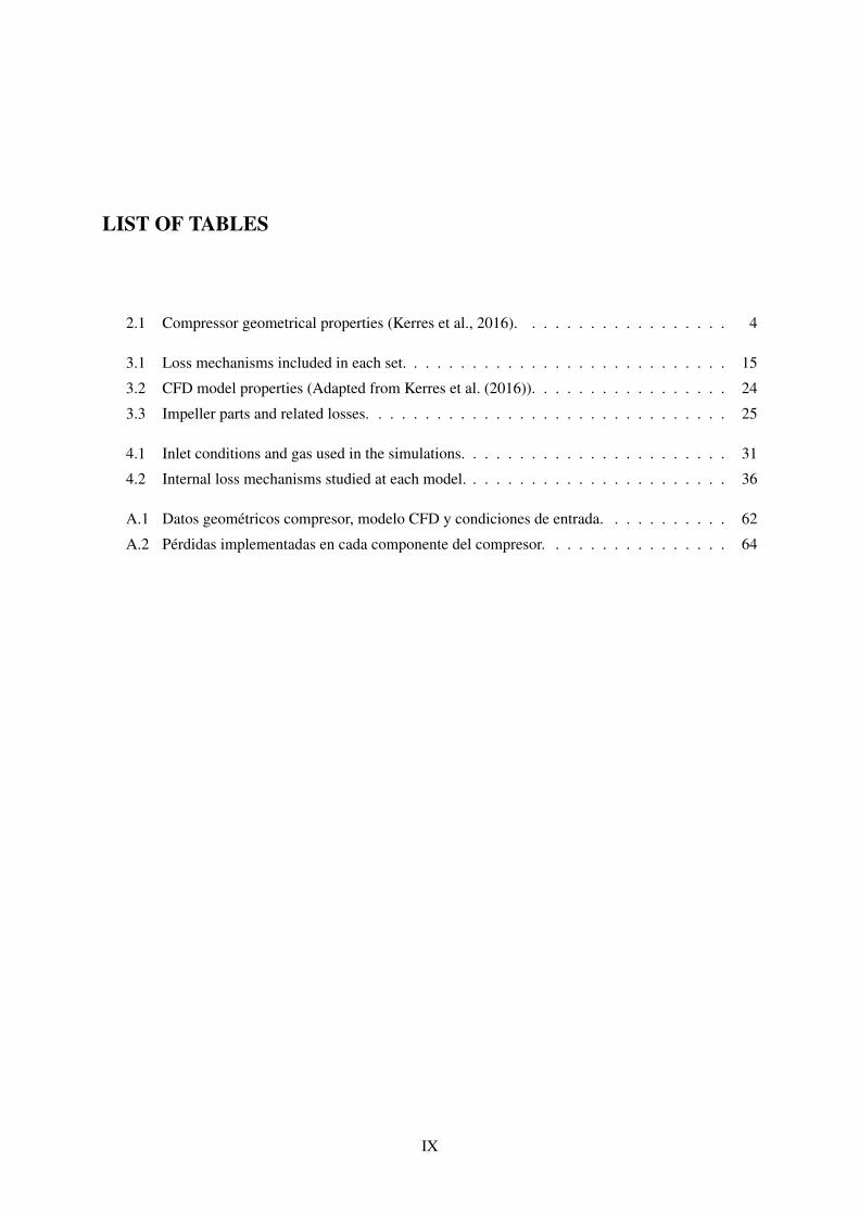
LIST OF TABLES IX
NOMENCLATURE X
1 INTRODUCTION. 11.1 Background. . . . . . . . . . . . . . . . . . . . . . . . . . . . . . . . . . . . . . . . . . 1
1.2 Purpose. . . . . . . . . . . . . . . . . . . . . . . . . . . . . . . . . . . . . . . . . . . . 2
1.3 Methodology. . . . . . . . . . . . . . . . . . . . . . . . . . . . . . . . . . . . . . . . . 2
2 FRAME OF REFERENCE. 32.1 Turbochargers: operating principle and components. . . . . . . . . . . . . . . . . . . . 3
2.2 Principles of compressor analysis. . . . . . . . . . . . . . . . . . . . . . . . . . . . . . 4
2.2.1 Blade work input coefficient. . . . . . . . . . . . . . . . . . . . . . . . . . . . . 8
2.3 One-dimensional centrifugal compressor model. . . . . . . . . . . . . . . . . . . . . . . 10
3 IMPLEMENTATION. 113.1 One-dimensional analysis. . . . . . . . . . . . . . . . . . . . . . . . . . . . . . . . . . 11
3.2 Impeller model. . . . . . . . . . . . . . . . . . . . . . . . . . . . . . . . . . . . . . . . 12
3.2.1 Aungier set of losses. . . . . . . . . . . . . . . . . . . . . . . . . . . . . . . . . 14
3.2.2 Oh et al.’s set of losses. . . . . . . . . . . . . . . . . . . . . . . . . . . . . . . . 19
3.3 Vaneless diffuser model. . . . . . . . . . . . . . . . . . . . . . . . . . . . . . . . . . . 20
3.4 Volute model. . . . . . . . . . . . . . . . . . . . . . . . . . . . . . . . . . . . . . . . . 22
3.5 CFD losses. . . . . . . . . . . . . . . . . . . . . . . . . . . . . . . . . . . . . . . . . . 24
3.5.1 Impeller losses. . . . . . . . . . . . . . . . . . . . . . . . . . . . . . . . . . . . 24
3.5.2 Vaneless diffuser and volute losses. . . . . . . . . . . . . . . . . . . . . . . . . 28
4 ANALYSIS AND RESULTS. 31
V

4.1 Overall stage predictions. . . . . . . . . . . . . . . . . . . . . . . . . . . . . . . . . . . 31
4.2 Impeller performance and losses prediction. . . . . . . . . . . . . . . . . . . . . . . . . 35
4.2.1 Blades work. . . . . . . . . . . . . . . . . . . . . . . . . . . . . . . . . . . . . 35
4.2.2 Internal losses. . . . . . . . . . . . . . . . . . . . . . . . . . . . . . . . . . . . 36
4.2.3 External losses. . . . . . . . . . . . . . . . . . . . . . . . . . . . . . . . . . . . 47
4.3 Vaneless diffuser performance and losses prediction. . . . . . . . . . . . . . . . . . . . 49
4.4 Volute performance and losses prediction. . . . . . . . . . . . . . . . . . . . . . . . . . 50
4.5 Losses breakdown. . . . . . . . . . . . . . . . . . . . . . . . . . . . . . . . . . . . . . 52
5 CONCLUSIONS AND FUTURE WORK. 555.1 Conclusions. . . . . . . . . . . . . . . . . . . . . . . . . . . . . . . . . . . . . . . . . . 55
5.2 Future work. . . . . . . . . . . . . . . . . . . . . . . . . . . . . . . . . . . . . . . . . . 56
APPENDICES 59
A RESUMEN EN ESPANOL DEL TRABAJO. 59A.1 Introduccion y objetivos. . . . . . . . . . . . . . . . . . . . . . . . . . . . . . . . . . . 59
A.1.1 Introduccion y marco de referencia. . . . . . . . . . . . . . . . . . . . . . . . . 59
A.1.2 Objetivos. . . . . . . . . . . . . . . . . . . . . . . . . . . . . . . . . . . . . . . 61
A.2 Implementacion. . . . . . . . . . . . . . . . . . . . . . . . . . . . . . . . . . . . . . . 62
A.2.1 Modelos unidimensionales. . . . . . . . . . . . . . . . . . . . . . . . . . . . . 62
A.2.2 Calculo de perdidas en el modelo CFD. . . . . . . . . . . . . . . . . . . . . . . 63
A.3 Analisis de resultados. . . . . . . . . . . . . . . . . . . . . . . . . . . . . . . . . . . . 66
A.3.1 Prediccion analıtica del rendimiento del compresor. . . . . . . . . . . . . . . . . 66
A.3.2 Suma de perdidas en cada componente. . . . . . . . . . . . . . . . . . . . . . . 68
A.3.3 Perdidas en el rotor. . . . . . . . . . . . . . . . . . . . . . . . . . . . . . . . . . 69
A.4 Conclusiones y lıneas futuras. . . . . . . . . . . . . . . . . . . . . . . . . . . . . . . . 71
REFERENCES 73
VI

LIST OF FIGURES
2.1 Turbocharger (Adapted from NASA). . . . . . . . . . . . . . . . . . . . . . . . . . . . 3
2.2 Centrifugal ompressor geometry. . . . . . . . . . . . . . . . . . . . . . . . . . . . . . . 4
2.3 Velocity triangles at the impeller inlet and outlet. . . . . . . . . . . . . . . . . . . . . . 5
2.4 Impeller control volume (Adapted from Kerres et al. (2016)). . . . . . . . . . . . . . . . 5
2.5 h-s diagram of a centrifugal compressor. . . . . . . . . . . . . . . . . . . . . . . . . . . 7
2.6 Compressor map (Adapted from Kerres (2014)). . . . . . . . . . . . . . . . . . . . . . . 8
3.1 Flow chart of the iterative calculation. . . . . . . . . . . . . . . . . . . . . . . . . . . . 12
3.2 Impeller calculation order applying Aungier pressure loss coefficients. . . . . . . . . . . 14
3.3 Impeller calculation order applying Oh et al. enthalpy loss coefficients. . . . . . . . . . . 14
3.4 Volute geometry. . . . . . . . . . . . . . . . . . . . . . . . . . . . . . . . . . . . . . . 23
3.5 Entropy field function. . . . . . . . . . . . . . . . . . . . . . . . . . . . . . . . . . . . 25
3.6 h-s diagram along an impeller part. . . . . . . . . . . . . . . . . . . . . . . . . . . . . . 26
3.7 h-s diagram between impeller inlet and outlet. . . . . . . . . . . . . . . . . . . . . . . . 27
3.8 Entropy field function. . . . . . . . . . . . . . . . . . . . . . . . . . . . . . . . . . . . 28
3.9 Vaneless diffuser and volute sections. . . . . . . . . . . . . . . . . . . . . . . . . . . . 29
4.1 Total pressure ratio. . . . . . . . . . . . . . . . . . . . . . . . . . . . . . . . . . . . . . 32
4.2 Relative TPR error between experimental measurements and 1D results. . . . . . . . . . 33
4.3 Total-to-total adiabatic efficiency. Red dashed lines = ±10% . . . . . . . . . . . . . . . 34
4.4 Dimensionless blades work coefficient prediction. . . . . . . . . . . . . . . . . . . . . . 35
4.5 Slip factor. . . . . . . . . . . . . . . . . . . . . . . . . . . . . . . . . . . . . . . . . . . 36
4.6 Internal loss coefficient. . . . . . . . . . . . . . . . . . . . . . . . . . . . . . . . . . . . 37
4.7 Incidence loss coefficient. . . . . . . . . . . . . . . . . . . . . . . . . . . . . . . . . . . 38
4.8 Inlet flow and blade angle. . . . . . . . . . . . . . . . . . . . . . . . . . . . . . . . . . 39
4.9 Skin friction loss coefficient. . . . . . . . . . . . . . . . . . . . . . . . . . . . . . . . . 39
4.10 Blade loading loss coefficient. . . . . . . . . . . . . . . . . . . . . . . . . . . . . . . . 40
4.11 Blade loading loss coefficient predicted by the one-dimensional models (without adding
hub-to-shroud losses). . . . . . . . . . . . . . . . . . . . . . . . . . . . . . . . . . . . . 41
4.12 Mixing loss coefficient. . . . . . . . . . . . . . . . . . . . . . . . . . . . . . . . . . . . 42
4.13 Entropy field at impeller tip. Negative values are reached since entropy is calculated by
comparing to a reference point. . . . . . . . . . . . . . . . . . . . . . . . . . . . . . . . 43
VII

4.14 Wake area ratio. . . . . . . . . . . . . . . . . . . . . . . . . . . . . . . . . . . . . . . . 43
4.15 Choking loss coefficient. . . . . . . . . . . . . . . . . . . . . . . . . . . . . . . . . . . 44
4.16 Tip clearance loss coefficient. . . . . . . . . . . . . . . . . . . . . . . . . . . . . . . . . 45
4.17 Shock loss coefficient. . . . . . . . . . . . . . . . . . . . . . . . . . . . . . . . . . . . 46
4.18 Distortion loss coefficient. . . . . . . . . . . . . . . . . . . . . . . . . . . . . . . . . . 46
4.19 External loss coefficient. . . . . . . . . . . . . . . . . . . . . . . . . . . . . . . . . . . 47
4.20 External losses in one-dimensional models. . . . . . . . . . . . . . . . . . . . . . . . . 48
4.21 Reverse mass flow percentage. . . . . . . . . . . . . . . . . . . . . . . . . . . . . . . . 48
4.22 Vaneless diffuser loss coefficient. . . . . . . . . . . . . . . . . . . . . . . . . . . . . . . 49
4.23 Volute funnel recovery coefficient. . . . . . . . . . . . . . . . . . . . . . . . . . . . . . 50
4.24 Volute cone loss coefficient. . . . . . . . . . . . . . . . . . . . . . . . . . . . . . . . . 51
4.25 Pressure loss coefficients in 1D volute funnel models. . . . . . . . . . . . . . . . . . . . 51
4.26 Losses breakdown (U2 = 0.62N0). . . . . . . . . . . . . . . . . . . . . . . . . . . . . . 53
4.27 Losses breakdown (U2 = 1.14N0). . . . . . . . . . . . . . . . . . . . . . . . . . . . . . 53
4.28 Losses breakdown (U2 = 1.41N0). . . . . . . . . . . . . . . . . . . . . . . . . . . . . . 53
A.1 Turbocompresor (Adaptado de NASA). . . . . . . . . . . . . . . . . . . . . . . . . . . 60
A.2 Geometrıa de un compresor centrıfugo. . . . . . . . . . . . . . . . . . . . . . . . . . . 60
A.3 Algoritmo de calculo en cada componente. . . . . . . . . . . . . . . . . . . . . . . . . . 63
A.4 Diagrama h-s para calculo de perdidas del rotor en el modelo CFD. . . . . . . . . . . . . 65
A.5 Volumenes de control tomados en el rotor. . . . . . . . . . . . . . . . . . . . . . . . . . 66
A.6 Ratio de presion total en cada modelo y experimental. . . . . . . . . . . . . . . . . . . . 67
A.7 Suma de perdidas internas a lo largo de cada componente. . . . . . . . . . . . . . . . . . 68
A.8 Perdidas en el rotor. . . . . . . . . . . . . . . . . . . . . . . . . . . . . . . . . . . . . . 70
VIII
LIST OF TABLES
2.1 Compressor geometrical properties (Kerres et al., 2016). . . . . . . . . . . . . . . . . . 4
3.1 Loss mechanisms included in each set. . . . . . . . . . . . . . . . . . . . . . . . . . . . 15
3.2 CFD model properties (Adapted from Kerres et al. (2016)). . . . . . . . . . . . . . . . . 24
3.3 Impeller parts and related losses. . . . . . . . . . . . . . . . . . . . . . . . . . . . . . . 25
4.1 Inlet conditions and gas used in the simulations. . . . . . . . . . . . . . . . . . . . . . . 31
4.2 Internal loss mechanisms studied at each model. . . . . . . . . . . . . . . . . . . . . . . 36
A.1 Datos geometricos compresor, modelo CFD y condiciones de entrada. . . . . . . . . . . 62
A.2 Perdidas implementadas en cada componente del compresor. . . . . . . . . . . . . . . . 64
IX

NOMENCLATURE
Latin letters.A Area
AR Area ratio
B Fractional area blockage
C Absolute velocity
Cr Throat contraction ratio
D Divergence parameter
D f Diffusion factor
I Work input term
L Length
M Mach number
PR Pressure ratio
Qc Corrected flow coefficient
R Gas constant
Re Reynolds numbers
Ro Rothalpy
SP Sizing parameter
T Temperature
U Tangential velocity
W Relative velocity
Z Number of blades
a Speed of sound
b Width
c f Skin friction coefficient
cp Specific heat capacity at constant pressure
d Diameter
dh Hydraulic diameter
e Wall roughness
fc Correction factor
fDF Disk friction factor
h Specific enthalpy
X

m Meridional coordinate
m Mass flow
p Pressure
r Radius
s Specific entropy
scl Blade-shroud clearance
t Bale width
y Distance from the wall
w Specific work
Greek lettes.Ωc Corrected angular speed coefficient
α Absolute flow angle to tangential direction
αc Flow angle to axial direction
β Relative flow angle to tangential direction
βb Blade angle to tangential direction
γ Heat capacity ratio
δ Boundary layer thickness
ε Radius ratio
εwake Wake area ratio
κm Streamline curvature
λ Enthalpy loss coefficient
λ dis Distortion factor
µ Viscosity
η Adiabatic efficiency
ρ Density
σ Slip facor
φ Flow coefficient
χ Wake mass flow ratio
ω Rotational speed
ω Dimensionless pressure loss coefficient
Subscripts.0 Total quantity
1 Impeller inlet
2 Impeller outlet
3 Diffuser outlet
4 Volute cone inlet
XI

5 Volute cone outlet
∞ Perfect guidance case
FB Full Blade
SB Splitter Blace
cl Blade-shroud clearance
ext External
h Hub
int Internal
m Meridional component
u Tangential component
r Relative quantity
s Isentropic condition
t Blade tip
th Throat parameter
0 Total quantity
Superscripts.() Average
()∗ Sonic conditions
()dc Design conditions
()L Loss
Acronyms.CFD Computational Fluid Dynamics
RANS Reynolds-averaged Navier–Stokes
XII

Chapter 1
INTRODUCTION.
1.1 Background.
Since the first turbocharger was invented in 1925 by the Swiss engineer Alfred Buchi, their importance inengines has been always growing. Nowadays, turbochargers are assembled in a lot of engines, from smallcommercial engines to racing F1 engines. The reason why turbochargers have become so important isthe downsizing trend.
Engine downsizing means making the engines smaller but keeping the same or even increasing the poweroutput. Higher efficiencies are obtained by downsizing due to the reduction of thermal and friction losses.These higher efficiencies reduces the fuel consumption and the emissions which are the main goalsbehind the downsizing process. To do it, modern technologies, such as turbocharging, direct injectionor variable timing valve, are added in the engine. This trend is very present nowadays and it can beseen how six-cylinder engines are replacing the eight ones, four-cylinders are replacing the six ones and,recently, the new three-cylinder engines are replacing fours (Squatriglia, 2016).
Turbocharging is one of the most common techniques used by manufacturers to achieve the enginedownsize. The aim of turbocharging is to increase the mass of air introduced into the cylinder duringthe intake stroke. More air means that more fuel can be burnt, increasing the power output per cycle.Furthermore, efficiencies are higher using turbocharges since the exhaust gas energy is used instead ofbeing lost as in atmospheric engines.
A design challenge is to design a engine-turbocharger system with a high level of matching in all rangeof different regimes. Therefore it is always desirable to obtain a mathematical model of it. Since aturbocharger consists of a turbine and a compressor, a model of each component need to be developedand coupled. These mathematical models allow to understand the system behaviour and performance,without needing too many expensive and long experiments.
This thesis describes an example of compressor model implementation. Nowadays, Computational FluidDynamics (CFD) software can run complex 3D models, getting accurate predictions. However, thesesimulations require long computational times and very expensive hardware. Since several decades ago,analytical models have been developed. These models make some assumptions that allows to predictwhole compressor maps in short times. Moreover, they need a relatively low number of input parameters.Therefore, they are a useful tool during the design process of the centrifugal compressor, and furthermore,in the design of the turbocharger and turbocharger-engine system.
1

ANALYTICAL PREDICTION OF TURBOCHARGER COMPRESSOR PERFORMANCE
Thanks to the studies carried out in the last decades, in the open literature it is possible to find differentmethodologies and correlations to develop analytical compressor models. In this thesis, two of thoseanalytical models are implemented and compared with experimental and numerical data.
1.2 Purpose.
The main goal of this thesis is the implementation of an analytical centrifugal compressor performanceprediction and to compare its results with numerical and experimental data. To do it a turbochargercompressor is used as reference. It consists of a impeller, a vaneless diffuser and a volute. Therefore,those are the modelled components.
To verify the validity of the model, its results are compared with experimental data, measuring the qualityof the compressor outputs predictions.
Finally, to further understand the model, another goal of the thesis is to compare the model losses withvalidated RANS data. The CFD model and simulations are already done and they are not a part of thisstudy. However, it is a task of this study to extract the losses from the CFD. This comparison shouldyields some conclusions about the strengths and weaknesses of the model.
1.3 Methodology.
Among the possible one-dimensional models that will be described in Chapter 2, the single-zone ap-proach is chosen since in the open literature it is possible to find several methodologies and correlationsto carry it out. Two different single-zone models are implemented in this thesis.
• The methodology described by Aungier (2000), which has been validated by hundreds of differentcompressor stages. Approaches and losses sets for all the compressor components are providedand, therefore, it is a very complete model.
• The impeller losses set provided by Oh et al. (1997), who provides this set after comparing 144different combinations of impeller losses with experimental data. The impeller loss correlationsused in this comparison are based on the work done by many authors.
Both models are implemented in MATLAB c© owing to its proper features to programme and calculateengineering and scientific problems. They are deeper explained in Chapter 3.
Once the model are implemented, the comparison with experimental data is done by calculating therelative error of the total pressure ratio and adiabatic efficiency in all the predicted points.
Finally, the model losses are compared with a validated CFD model. This model is done in STAR-CCM+ c©. Due to the complexity of the flow, some assumptions are done to independently measure somelosses. Then, the comparison is done by analysing the trend and values range of each loss across thewhole compressor map.
2

Chapter 2
FRAME OF REFERENCE.
2.1 Turbochargers: operating principle and components.
A brief description of how turbocharger works is explained in the next paragraphs. In the literature canbe easily found many books about them, such as Payri and Desantes (2011).
Turbochargers are turbine-driven forced induction devices that increase engine efficiency and poweroutput. A turbocharger consists of a centrifugal compressor and a radial turbine joined by a commonshaft (Figure2.1). Exhaust gasses of the engine flow through the turbine. The turbine uses the thermalfluid energy to drive the compressor through the common shaft. Then, the compressor takes atmosphericair, increases its pressure and sends it to the engine’s intake. Since the air pressure and density are higherthe amount of air that is introduced in the engine is larger. Therefore, the engine can generate more powerthrough the combustion of more air and fuel. Efficiency also increases due to the higher compressionratio reached.
TURBINE
CENTRIFUGAL
COMPRESSOR
COMMON
SHAFT
Figure 2.1: Turbocharger (Adapted from NASA).
3

ANALYTICAL PREDICTION OF TURBOCHARGER COMPRESSOR PERFORMANCE
Because of this thesis is focused on the centrifugal compressor, just this component is described in depth.Figure 2.2 shows the main parts of a compressor. First the impeller is rotating thanks to the power appliedon the shaft and the fluid flows across it. The impeller blades have a specific passage between them thatincreases the fluid pressure and reduces its relative velocity. After leaving the impeller, the flow goes intothe diffuser which further increases its pressure and decelerates it more. The diffuser can be vaneless orvaned, although vaneless diffusers are more common in turbochargers due to their wider operation range.Finally, the flow goes through the volute where pressure rises more and the velocity is adapted to the exitrequirements.
ω
ω
VOLUTE
VANELESS
DIFFUSER
VOLUTE
CONE
VOLUTE
FUNNEL
IMPELLER
HUB
BLADE
PASSAGE
IMPELLER
SHROUD
IMPELLER
BLADE
Figure 2.2: Centrifugal ompressor geometry.
The compressor analysed in this thesis is a compressor for a passenger car turbocharger. Its main geo-metrical properties are summarizes in Table 2.1.
Table 2.1: Compressor geometrical properties (Kerres et al., 2016).
Compressor geometryExducer diameter 52.5mmNumber of full blades 6Number of splitter blades 6Diffuser Area Ratio AR=0.708Mass flow coefficient φ dc=0.094Work coefficient ϕdc=0.622Blade Mach number Mdc
2 =1.09
2.2 Principles of compressor analysis.
In this section, a brief study of the principles of compressors is carried out. This analysis can be foundin many turbomachinery book. The books of Cumpsty (2004) and Korpela (2011) have been the maintheoretical references used in this study.
The interaction between the blades and the flow is the essential process of the compressor operation. Bythis interaction, the work is transferred from the blades to the flow. It is convenient to study the flowvelocity at the inlet and at the outlet in order to obtain the work applied on the shaft. To do it, velocitytriangles are developed examining the flow in a stationary frame and in a moving one that rotates at the
4

CHAPTER 2. FRAME OF REFERENCE.
same angular speed as the impeller. Fig. 2.3 shows these velocity triangles of a backswept centrifugalimpeller assuming that the inlet flow has no radial component and, at the outlet, it has no componentin the axial direction. The absolute velocities in the stationary frame are denoted by C, while relativevelocities by W and the speed due to the rotation of the moving frame by U. Besides, the angles that theabsolute and relative velocities form with the tangential direction are denoted by α and β respectively.These flow angles are called absolute and relative flow angles. Subscripts u and m respectively denotetangential and meridional components.
C1
β1
α1
U1
W1
(a) Inlet velocities.
Cm2
α2β2
W2 C2
U2
(b) Outlet velocities.
Figure 2.3: Velocity triangles at the impeller inlet and outlet.
Considering now the flow through the impeller as shown in Fig. 2.4 and taking a control volume thatincludes both the impeller and the fluid, it is possible to calculate the work transferred. To obtain it,angular momentum balance is applied and the torque input on the shaft is
Cm1
Cu1
Cm2
τ
Cu2
Figure 2.4: Impeller control volume (Adapted from Kerres et al. (2016)).
τ = m(r2Cu2− r1Cu1) (2.1)
m being the mass flow, r2 and r1 the mean outlet and inlet radius and Cu the tangential velocity. Multi-plying the torque by the angular speed ω and dividing it by the mass flow, the power input per unit massis
w = ω(r2Cu2− r1Cu1) (2.2)
5

ANALYTICAL PREDICTION OF TURBOCHARGER COMPRESSOR PERFORMANCE
Finally, taking into account that the blade speed (U) is equal to U = rω , Formula 2.2 can be recasted andit leads to Euler equation of turbomachinery is obtained.
w =U2Cu2−U1Cu1 (2.3)
Experiments show that some phenomena, such as slip or inlet distortion, decrease the real blade inputwork comparing to the Euler’s formula. Analytical approaches introduce some empirical factor to modelthem. They are explained subsequently in Section 2.2.1.
It is important to continue the analysis going into the thermodynamic involved. It will allow to relate thepower input and flow velocities with the fluid properties (mainly temperature and pressure).
The first law of thermodynamics is applied to the same volume control than before. Since turbomachineryflows are almost adiabatic and the potential energy variation in gas flows can be neglected, the work inputper unit mass is
w = h2 +12
C22−h1 +
12
C21 (2.4)
being h the static enthalpy. Defining the stagnation enthalpy (h0) as the sum of the static enthalpy and
the kinetic energy (h0 = h+12
C2), Equation 2.4 can be simplified as follows.
w = h02−h01 (2.5)
It is seen how the work applied on the shaft is absorbed by the fluid increasing its stagnation enthalpy.Through the Euler equation and Equation 2.4, the next equation is obtained.
Ro = h2−U2Cu2 = h1−U1Cu1 (2.6)
The parameter Ro is called rothalpy. It is seen that is constant across the impeller. Rearranging Formula3.2 leads to
h2−h1 =12(U2
2 −U21 )+
12(W 2
1 −W 22 ) (2.7)
Equation 2.7 shows how static enthalpy and pressure rise can be achieved across the impeller by twomethods: a) increasing the centrifugal effect (first term) or b) decelerating the relative flow (secondterm) (Korpela, 2011). While the deceleration process produces some losses, the pressure rise by thecentrifugal effect (U2 > U1) is a loss-free process. This fact has favoured the developed of centrifugalcompressors due to reasonable large efficiencies can be reached even without high aerodynamic perfor-mance. The flow at the exit of the impeller has usually large absolute velocity and that is why a diffuseris needed afterwards. The diffuser decelerates the flow further increasing the pressure more. Finally, thevolute continues decelerating and rising the pressure. It is convenient to analyze the whole process in ah-s diagram. Figure 2.5 shows it. Label 1 and 2 represent the impeller inlet and outlet, while label 3 in-dicates the diffuser outlet and label 5 the volute outlet. Label 4 is reserved in this thesis to a intermediatevolute point.
The diagram shows both the adiabatic process line (from 1 to 5) and the isentropic process line (from 1to 5s). Comparing the work input with the necessary work to reach the same exit pressure but followingan isentropic process, the total-to-total efficiency can be defined as
ηtt =ws
w=
h03s−h01
h03−h01(2.8)
6

CHAPTER 2. FRAME OF REFERENCE.
Δht
01
02
p02
p01
h
s
h02=h03 =h05
h01
Δhs
03
p03 p05
05
05s
Figure 2.5: h-s diagram of a centrifugal compressor.
This efficiency in centrifugal compressor is usually between 0.70-0.85 (Campbell, 1992).
Apart from the h-s diagram, the compressor map is also useful to characterize the compressor perfor-mance. It usually shows the pressure ratio as a function of the flow. Efficiency and constant speed curvesare also plotted. Corrected coefficients of the flow and angular speed are used and they are defined below.
Qc = Q
√T0r
T01Ωc = Ω
√T0r
T01
These corrected coefficients come from the flow coefficient (φd =m√
RT01
p01d2 ) and the blade Mach number
(ωd√γRT01
)for compressive flows. These last non-dimensional coefficients are used in the similitude stud-
ies of turbomachinery, which are powerful tools to compare the performance of two turbomachines or toforecast the performance of a turbomachine from its prototype’s outputs (Korpela, 2011). Corrected co-efficients are not dimensionless since they are derived from the flow coefficient and blade Mach numberbut particularizing for a specific fluid and compressor design. Therefore, corrected coefficient are usedto compare different working conditions of the same compressor.
Figure 2.6 shows an example of a compressor map. It is seen that there are two regions where thecompressor can not operate in normal conditions. Above the surge line, the blades will stall and aphenomena called surge may appear. Even though there are different types of stall, their consequencesare much less severe than the surge ones. In centrifugal compressors it is possible to operate under stableconditions with stall present, although the efficiency and pressure rise are lower (Cumpsty, 2004). On thecontrary, surge generally produces an unstable and unacceptable operation with high flow and pressureoscillations and reverse flows. Apart from this oscillations, surge usually produces vibration and anaudible sound that make it easily detectable. However, this vibration may reach excessive amplitudesand frequencies causing catastrophic effects on the whole system (Boyce et al., 1983). After many yearsof research on this field, there is still a great controversy about the cause and relation between stalland surge. Moreover, divergence of these results is increased due to surge and stall patterns have been
7

ANALYTICAL PREDICTION OF TURBOCHARGER COMPRESSOR PERFORMANCE
demonstrated to be quite diverse from one compressor to another (Zheng and Liu, 2015). In the otherside of the compressor map, when the mass flow reaches very high values, the flow is chocked and it isnot possible to increase further the mass flow causing a sharp drop of the constant speed lines.
SURGE LINE
CHOKE LINE
Isoefficiency
Speed line (Ωc)
Corrected volumetric flow coefficient (Qc)
Pre
ssu
re R
ati
o
Figure 2.6: Compressor map (Adapted from Kerres (2014)).
2.2.1 Blade work input coefficient.
IB denotes the dimensionless blade work input coefficient. It is derived from Euler’s formula (Equation2.3).
IB =Cu2/U2−U1Cu1/U22 (2.9)
If the flow was perfectly guided by the blades, Cu2 would be equal to Cu2∞ =U2−Cm cotβ2b (see Figure2.39. However, the real tangential flow velocity is slightly less than that. This loss is called slip. Itis caused by the relative eddy rotation in a direction opposite to the impeller that appears to remainsthe flow irrotational in the absolute frame of reference. Therefore, a perfect blade guidance can not beconsidered and a slip factor σ is introduced in the analytical study. It is described as
σ =Cu2
Cu2∞
(2.10)
8

CHAPTER 2. FRAME OF REFERENCE.
This slip factor has been investigated for several decades and a large number of correlations have beendeveloped, such as the provided by Stodola (1945), Busemann (1928), Wiesner (1967) or the recentmodel done by Qiu et al. (2007). Wiesner’s model is used in this thesis as it is done by Aungier (2000).Following this model, the slip factor is described as
σ = 1−sinαC2
√sinβ2b
z0.7 (2.11)
where z denotes the number of vanes. The impeller usually has splitter blades. In those cases, the numberof blades are corrected by Z = ZFB +ZSBLSB/LFB.
Following the work done by Busemann (1928) and Wiesner (1967), (Aungier, 2000) introduces a cor-rection procedure that considered the slip factor as constant up to a certain radius ratio (εLIM). At largerε , slip ratio sharply falls. Therefore, slip ratio is calculated as follows.
ε = r1/r2
σ∗ = sin(19+0.2sinβ2b)
εLIM =σ −σ∗
1−σ
σ = 1−sinαC2
√sinβ2b
Z0.7 ; ε ≤ εLIM
σCOR = σ
1−(
ε− εLIM
1− ε
)√β2b/10 ε > εLIM
(2.12)
On the other hand, (Aungier, 2000) also provides a distortion factor (λ dis) that accounts for the impellertip blockage (B2). Both parameters are related as follows.
λdis =
11−B2
(2.13)
Aungier (1995) offers an empirical correlation to calculate B2 that fits a wide range of compressor per-formance. This correlation is
b2 = ωSFpv1
pv2
√W1dh
W2bh+[0.3+
b22
L2B]A2
Rρ2b2
ρ1LB+
sCL
2b2(2.14)
where pv = p0− p and AR = A2 sinβ2b/(A1 sinβth).
Therefore, taking into account Equation 2.9, the slip factor (σ ) and the tip distortion factor (λ dis), theblade work input coefficient is described as (Aungier, 2000).
IB = σ(1−λdis
φ2 cotβ2b)−U1Cu1/U22 (2.15)
9

ANALYTICAL PREDICTION OF TURBOCHARGER COMPRESSOR PERFORMANCE
2.3 One-dimensional centrifugal compressor model.
Thanks to the researches done in the last decades, several one-dimensional approaches have been devel-oped to estimate centrifugal compressor performance. These analytical models make different assump-tions to provide a whole compressor map prediction in short time. Depending on the assumptions made,one-dimensional models can be classified by the number of flow zones studied, as shown in Harley et al.(2013), Schneider et al. (2015) or Kerres et al. (2016). Therefore, one-dimensional models can be dividedinto the next three categories: zero-zone, single-zone and two-zone analyses.
Zero-zone approach can be applied at the earliest design stage but it shows the lowest level of detail. Anexample of this model is the recent analysis implemented by Casey and Robinson (2013). It assumesthat compressors for the same purpose have similar design and performance. Therefore, it comparesthe dimensionless flow coefficient, work coefficient and blade Mach number at the design point withthe coefficients of another similar compressor whose map is completely known. Then, the whole mapof the studied compressor is estimated by extrapolating all the off-design conditions from the referencecompressor map and the relation between the dimensionless coefficients.
Single-zone models go further and they focus on the main stream line. Assuming uniform flow at everysection, conservation of mass, momentum and energy are applied. Rothalpy conservation is also appliedin the impeller in order to estimate the work input. Finally, some experimental correlation losses areintroduced to calculate the real flow conditions. Therefore, this approach needs more geometry informa-tion than zero-zone models but the level of detail reached is higher, being possible to separately studyeach component performance. In order to implement single-zone models, several loss sets have beendeveloped during the last decades, such as the sets of Galvas (1974), Aungier (1995), Oh et al. (1997) or(Gravdahl and Egeland, 1999).
Finally, two-zone approach is based on the jet-wake flow profile at the impeller tip. The reference isthe study done by Dean and Senoo (1960). Jet flow appears at the pressure blade surface and it isassumed to be loss-free. Therefore, all the losses are concentrated in the high entropy wake flow thatappears close the suction surfaces. Both flows are separately calculated, applying conservation of mass,momentum and energy to each one. Loss correlations similar than the single-zone sets are applied tothe wake. Finally, a jet-wake mixing process is computed. Additional input data is required in thesemodels comparing to the zero- and single-zone approaches. Specially, some relations to estimate the jetand wake areas are needed. The most common methodologies are based on the definition of the massflow fractions or the velocity ratio as proposed by van den Braembussche (2013). Schneider et al. (2015)provides a two-zone turbocharger compressor model by applying a constant velocity ratio of 0.2. On theother hand, Oh et al. (2001) develops a two-zone model based on an empirical correlation that relates thewake mass flow fraction to the wake area fraction.
As it was said in Section 1.3, the single-zone models carried out by Aungier (2000) and Oh et al. (1997)are the ones implemented in this thesis. The reasons are already explained in Section 1.3.
10

Chapter 3
IMPLEMENTATION.
3.1 One-dimensional analysis.
Due to the development of one-dimensional compressor’s model that has been carried out during the lastdecades, some different procedures and losses set have been built up. As it was said before, this thesisis focused on the methodology developed by Ronald H. Aungier (2000) and Oh et al. (1997). They havebeen implemented in MATLAB c© owing to its proper features to programme and calculate engineeringand scientific problems.
Following the modularity that is characteristic of these procedures, each component is separetaly mod-elled. To develop the full compressor’s model they are connected in series afterwards. Thus, the outletsof one component are the inlets of the next one as in a real compressor. This modularity leads into alarge flexibility since several different compressor’s setups can be analyzed just changing the compo-nents added and the order in which they are connected.
To model each component, the geometry data and the model of the losses that affect along it are needed.The losses models are usually experimental correlations due to the difficulty to explain them by theo-retical equations. Besides, it will be seen in the next sections how these experimental correlation areusually a function of the conditions at the component outlet. Since the outlet conditions are obviously afunction of the losses too, an iterative procedure is needed. Therefore, each component’s performance iscalculated as follows.
• First, the thermodynamic conditions and velocity triangles at the inlet are obtained. In the case ofthe impeller, inlet conditions are equal to inlet compressor conditions. In the other components,as it was said before, inlet conditions are equal to the conditions at the outlet of the componentbefore.
• Then, outlet meridional velocity is guessed. In the case of the impeller, flow coefficient (Φ =m
ρ2A2U2) is guessed.
• After that, thermodynamic, fluid and turbomachinery equations are applied to calculate all thelosses coefficients. Once the pressure losses are known, outlet conditions are obtained.
• Then, it is checked if there is convergence of mass flow. If the error is not small enough, theoutlet meridional velocity or the flow coefficient is updated and the process is done again untilconvergence is reached.
• Finally,in the case of the impeller, external losses are applied as an enthalpy increment at constantpressure and the outlet conditions are updated.
11

ANALYTICAL PREDICTION OF TURBOCHARGER COMPRESSOR PERFORMANCE
Figure 3.1 shows this iterative procedure, similar to the one presented by Aungier (2000). It can be seenhow the analysis finishes when ’choke’ condition is reached. This condition is more general than realaerodynamic choke, e.g. when impeller efficiency is lower than 10% (Aungier, 2000). Even though vane-less diffuser can be calculated by the same iterative process, Aungier (1993) proposes a one-dimensionalperformance analysis based on four governing differential equations. Therefore, this iterative solutionwill be applied at the impeller and volute. The vaneless diffuser calculation will be explained later.
Geometry
Inlet conditions
Working conditions
Compute inlet absolute
and relative conditions.
Compute outlet ideal
relative conditions
(Aungier).
Tip Mass
Balance?
Compute blades work and
internal losses.
Compute tip absolute
flow.
Guess meridional velocity
/ tip flow coefficient
Choke?
Adjust mer.
veloticy / tip flow
coeff.
Compute External LossesCompute tip absolute
flow.
End
End
End
No
Yes
Yes
No
ImpellerNo impeller
Figure 3.1: Flow chart of the iterative calculation.
3.2 Impeller model.
Since Aungier describes the losses by pressure loss coefficients while Oh et al. described them byenthalpy losses there is a slight different between both calculations. On one hand, Aungier’s impelleranalysis is mostly carried out on a rotating frame of reference that rotates at the rotor speed. Therefore,several relations between the relative and static conditions must be known. The first one is based on thefact that static enthalpy is the same in both frames of reference. It leads to Equation 3.1.
h = h0r−W 2
2= h0−
C2
2(3.1)
The subscript r means relative property. Defining the relative Mach number as Mr =Wa
and takinginto account Equation 3.1 and isentropic relations between the static and total relative conditions, thefollowing equations are obtained (Aungier, 1995).
T0r = T [1+γ−1
2M2
r ] (3.2)
p0r = p[1+γ−1
2M2
r ]
γ
γ−1 (3.3)
12

CHAPTER 3. IMPLEMENTATION.
Through the last equations, thermodynamic equations and velocity diagrams all the impeller conditionsat the inlet can be easily known.
To calculate the outlet properties, once a flow coefficient is guessed, the isentropic outlet relative condi-tions are computed by the proper isentropic relations, equation of state, velocity diagrams and conserva-tion of rothalpy, Ro, across the impeller. Rothalpy is defined as the difference between the total enthalpyand angular momentum and its conservation in a relative frame of reference leads to the next equation.
Ro = h0−ωrCu = const.
h02r = h01r +(U22 −U2
1 )/2 (3.4)
Non-isentropic outlet properties are obtained afterwards. To do it, the outlet relative total pressure iscalculated by Equation 3.5 (Aungier, 1995).
p02r = p02r,s− fc(p01r− p1)∑i
ωi (3.5)
where ωi are the different pressure loss coefficients that will be explained later. fc is a correction factorneeded to remain the entropy rise unchanged. It is defined as follows.
fc =ρ02rT02r
ρ01rT01r(3.6)
The discharge relative total temperature is easily calculated by Equation 3.4. Besides, the outlet totaltemperature is obtained by Euler’s formula (Equation 2.3) that leads to
T02 = T01 +IBU2
2cp
(3.7)
Once the outlet relative total conditions are known, total and static absolute conditions are computed byapplying isentropic relations, equation of state and velocity diagrams.
On the other hand, the Oh et al. model is carried out mainly in the stationary frame of reference. There-fore, the isentropic outlet total enthalpy is calculated first by guessing an outlet flow coefficient, comput-ing the blades work coefficient and applying the sum of all the enthalpy losses as follows.
h02,s = h01 + IBU22 −∑
i∆hL
i (3.8)
Isentropic and non-insentropic outlet total temperature are directly computed by Equations 3.8 and 3.7respectively, dividing them by the specific heat capacity. Discharge total pressure is then given by
p02 = p01
(T02,s
T01
)( γ
γ−1
)(3.9)
The rest of total and static outlet conditions are calculated by isentropic relations, equations of state andvelocity diagrams.
Once mass flow convergence is reached, parasitic work terms (Ii =∆hext
0
U22
), such as the disk friction
work or the recirculation work, are computed and applied at constant pressure in both models. Finally,
13

ANALYTICAL PREDICTION OF TURBOCHARGER COMPRESSOR PERFORMANCE
tip conditions are adjusted to this new enthalpy. Figure 3.2 and 3.3 show the different thermodynamicpoints that are involved within these processes and the order in which they are calculated. Not all the
Δhb=IBU22
b
02
p02
p01
h
s
h02
h0b
h01
Δhext
1
4
5
(a) Stationary frame of reference.
Δhr=(U22-U1
2)
b
02
p02r
h
s
h02r
h0br
1
3
bs
2
P02r,s
p01rh01r
(b) Relative frame of reference.
Figure 3.2: Impeller calculation order applying Aungier pressure loss coefficients.
Δhb=IBU22
b
02
p02
p01
h
s
h02
h0b
h01
Δhext
1
3
4
2
ΣΔhint
Figure 3.3: Impeller calculation order applying Oh et al. enthalpy loss coefficients.
internal losses that are taken into account at one losses set are implemented in the other set. Table 3.1summarizes the losses included at each model. Both sets are explained in the next sections,
3.2.1 Aungier set of losses.
Incidence loss. At the leading edge, the flow is adjusted to the blade angle causing a pressure loss. Thisloss can be modelled as (Aungier, 2000).
ωinc = 0.8[1−Cm1/(W1 sin(β1b)]2 +[ZFBtb1/(2πr1 sin(β1b))]
2 (3.10)
ZFB being the number of full blades and tb1 the blade thickness at the inlet.
The overall incidence loss is calculated by a weighted average of its value at the hub, mean and shroud.To calculate the values at the hub and shroud, Cm1 must be corrected applying Equations 3.11. The mean
14

CHAPTER 3. IMPLEMENTATION.
Table 3.1: Loss mechanisms included in each set.
Aungier’s set Oh et al.’s setInternal Losses
Incidence x xSkin friction x x
Blade-loading x xWake-mixing x x
Clearance x xHub-to-shroud x
Choking xSupercritical Mach x
Distortion xExternal losses
Disk friction x xRecirculation x x
Leakage x x
value is weighted 10 times as heavy as the hub and shroud values (Aungier, 2000).
Cmh1 =Cm1[1+κm1b1/2]
Cmt1 =Cm1[1−κm1b1/2] (3.11)
where κm denotes the streamline curvature.
Choking loss. When the Mach number at the throat approximates values of 1.0, some losses are causedbecause of the proximity to the choke conditions. To model these losses, first a contraction ratio correla-tion is calculated in order to model the aerodynamic blockage at the throat (Aungier, 2000).
Cr =√(A1 sinβ1b/Ath); Cr ≤ 1− (A1 sinβ1/Ath−1)2 (3.12)
The choking loss is modelled as
X = 11−10CrAth/A∗
ωCH = 0; X ≤ 0
ωCH = 0.5(0.05X +X7); X ≥ 0(3.13)
where A∗ denotes the area for which sonic conditions would be reached. Dixon and Hall (1961) providesthe next equation to calculate the impeller critical area.
mA∗
= ρ01a01(2+(γ−1)U2
2 /a201
γ +1)
γ +12(γ−1) (3.14)
15
ANALYTICAL PREDICTION OF TURBOCHARGER COMPRESSOR PERFORMANCE
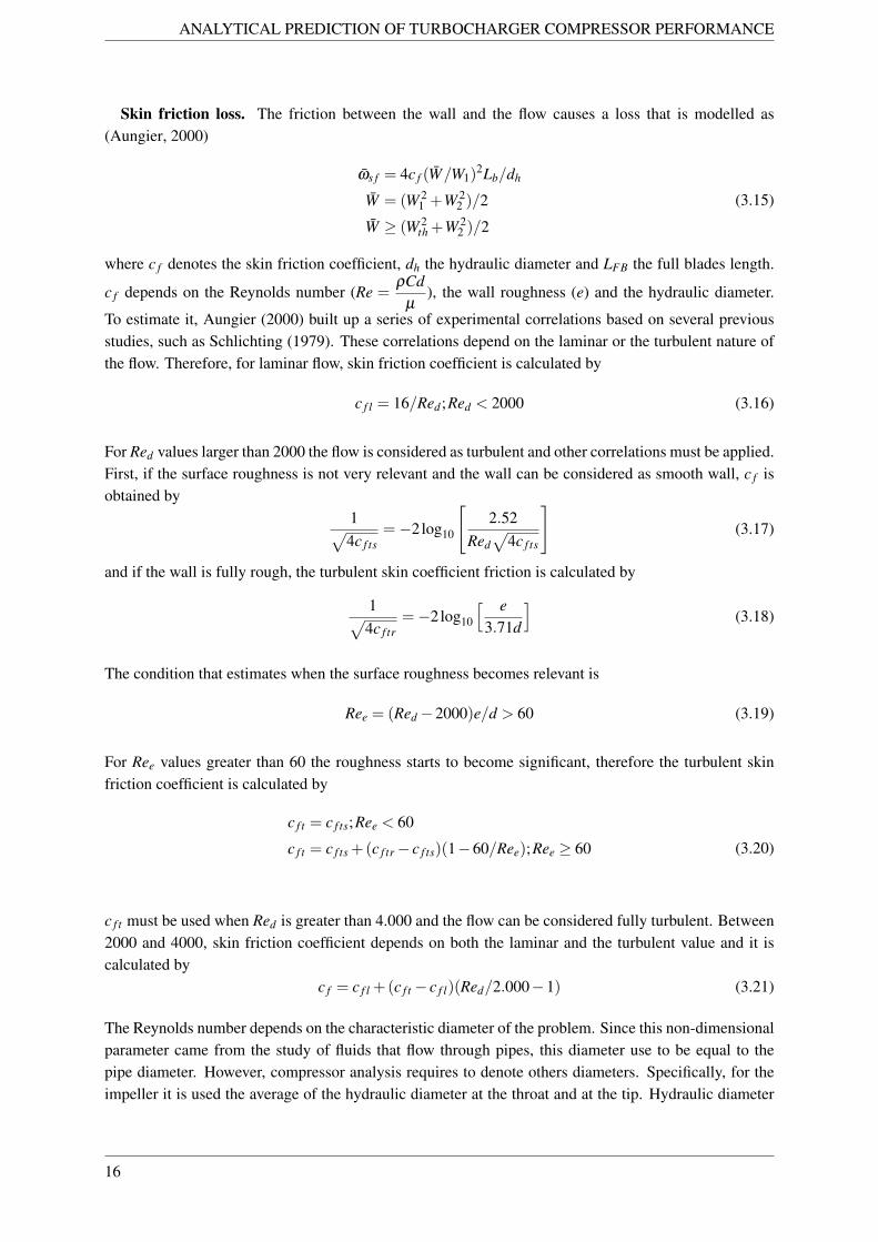
Skin friction loss. The friction between the wall and the flow causes a loss that is modelled as(Aungier, 2000)
ωs f = 4c f (W/W1)2Lb/dh
W = (W 21 +W 2
2 )/2
W ≥ (W 2th +W 2
2 )/2
(3.15)
where c f denotes the skin friction coefficient, dh the hydraulic diameter and LFB the full blades length.
c f depends on the Reynolds number (Re =ρCd
µ), the wall roughness (e) and the hydraulic diameter.
To estimate it, Aungier (2000) built up a series of experimental correlations based on several previousstudies, such as Schlichting (1979). These correlations depend on the laminar or the turbulent nature ofthe flow. Therefore, for laminar flow, skin friction coefficient is calculated by
c f l = 16/Red ;Red < 2000 (3.16)
For Red values larger than 2000 the flow is considered as turbulent and other correlations must be applied.First, if the surface roughness is not very relevant and the wall can be considered as smooth wall, c f isobtained by
1√4c f ts
=−2log10
[2.52
Red√
4c f ts
](3.17)
and if the wall is fully rough, the turbulent skin coefficient friction is calculated by
1√4c f tr
=−2log10
[ e3.71d
](3.18)
The condition that estimates when the surface roughness becomes relevant is
Ree = (Red−2000)e/d > 60 (3.19)
For Ree values greater than 60 the roughness starts to become significant, therefore the turbulent skinfriction coefficient is calculated by
c f t = c f ts;Ree < 60
c f t = c f ts +(c f tr− c f ts)(1−60/Ree);Ree ≥ 60 (3.20)
c f t must be used when Red is greater than 4.000 and the flow can be considered fully turbulent. Between2000 and 4000, skin friction coefficient depends on both the laminar and the turbulent value and it iscalculated by
c f = c f l +(c f t − c f l)(Red/2.000−1) (3.21)
The Reynolds number depends on the characteristic diameter of the problem. Since this non-dimensionalparameter came from the study of fluids that flow through pipes, this diameter use to be equal to thepipe diameter. However, compressor analysis requires to denote others diameters. Specifically, for theimpeller it is used the average of the hydraulic diameter at the throat and at the tip. Hydraulic diameter
16

CHAPTER 3. IMPLEMENTATION.
is defined as
dh = 4(cross− sectional area)(wetted perimeter)
(3.22)
Blade loading loss. Due to the pressure gradient in the blade-to-blade direction, secondary flows areproduced. These flows cause losses and they also may yield to impeller stall. The blade loading loss ismodelled by (Aungier, 2000)
ωbl = (∆W/W1)2/24 (3.23)
where ∆W is∆W = 2πd2U2IB/(ZLFB) (3.24)
Hub-to-shroud loading loss. This loss is similar to the blade loading loss, but it is caused by the pressuregradient in the hub-to-shroud direction. Its effects are similar and it is modelled by (Aungier, 2000)
ωHS = (κm ¯bW/W1)2/6
κm = (αC2−αC1)/LFB
b = (b1 +b2)/2
ω = (W1 +W2)/2
(3.25)
Distortion loss. Accounts for the mixing of the distorted meridional flow and the free stream flow.Following an abrupt expansion loss (Benedict et al., 1966), this loss is modelled by
ωλ = [(λ dis−1)Cm2/W1]2 (3.26)
Wake mixing loss. Aungier (1995) proposes that this loss caused by the mixing of the blade wake flowand the free steam flow can also be predicted by an abrupt expansion. First, the velocity at which theflow is separated must be predicted. It is calculated by Equations 3.27 where D f ,eq denotes an equivalentdiffusion factor and it is defined as D f ,eq =Wmax/W2. Wmax denotes the maximum relative reached in theblade passage and it is equal described as Wmax = (W1 +W2 +∆W )/2. ∆W is the average blade velocitydifference and it is estimated by ∆W = 2πd2IB/(ZLFB).
WSEP =W2; D f ,eq < 2
WSEP =W2D f ,eq/2; D f ,eq ≥ 2 (3.27)
The velocities before and after mixing are calculated as follows.
Cm,wake =√
W 2SEP−W 2
U
Cm,mix =Cm2A2/(πd2b2) (3.28)
Finally, the loss coefficient is estimated by
ωmix = [(Cm,wake−Cm,mix)/W1]2 (3.29)
17

ANALYTICAL PREDICTION OF TURBOCHARGER COMPRESSOR PERFORMANCE
Clearance gap leakage loss. Loss caused in open impeller due to the fluid that flows though the clear-ance between the blades and the shroud. It is modelled as (Aungier, 2000)
ωcl = 2mcl∆pcl/(mρ1W 21 ) (3.30)
where mcl and ∆pcl are the mass leakage flow and the pressure gradient across the gap respectively. Tocalculate both parameters, Aungier (1995) provides the next correlations. First, the leakage flow velocityis estimated as
Ucl = 0.816√
2∆pcl/ρ2 (3.31)
where the factor 0.816 is derived by assuming an abrupt expansion and an abrupt contraction later whenthe fluid flows through the blades clearance. The leakage flow is predicted by
mcl = ρ2sCLZLLBUcl (3.32)
s being the blade-shroud clearance. The pressure gradient is estimated as
∆pcl =m(r2Cu2− r1Cu1)
ZrbLB
r = (r1 + r2)/2
b = (b1 +b2)/2(3.33)
Supercritical Mach number loss. Shocks appears on the blade suction surface when the flow reachessupersonic conditions. When it happens, losses are generated and boundary layer separation may happen.Supercritical Mach number loss coefficient is described as (Aungier, 2000)
ωcr = 0.4[(M′1−M′cr)Wmax/W1]2 (3.34)
where M′cr is the inlet Mach number when sonic conditions are reached at the midpassage suction surface.It is predicted by (Aungier,1995)
M′cr = M′1W ∗/Wmax (3.35)
Disk friction loss. The friction between the impeller and the fluid that flows through the clearance gapscauses an external loss. This leads in a increment of input work which is not used to raise the fluidpressure. Nece and Daily (1960) provides the next equation to predict disk friction losses.
IDF =∆hL
0DF
U22
= fd fρr2
2U2
4m
ρ = (ρ1 +ρ2/2
fd f = 2.67/Re0.5d f ; Red f < 3 ·105
fd f = 0.0622/Re0.2d f ; Red f ≥ 3 ·105
Red f =U2r2/ν2
(3.36)
Recirculation loss. Some impellers show a significant raise in work input when working at low mass
18

CHAPTER 3. IMPLEMENTATION.
flow. This is caused by fluid that flow back into the impeller tip (Aungier, 2000). Aungier (1995) modelsthis loss by an empirical correlation as follows.
IRC = (D f ,eq/2−1)(Wu2/Cm2−2cotβ2); IRC ≥ 0
D f ,eq =Wmax/W2 (3.37)
D f ,eq is the equivalent diffusion factor provided by Lieblen (1959). It is developed for axial compressorbut it can be generalized to impellers. Lieblen predicts blade stall and thus flow recirculation whenD f ,eq > 2.
Leakage loss. The leakage flow that passes through the blade-shroud gap losses energy and it is reener-gized again. Aungier (2000) describes this loss assuming that half of the leakage flow suffers this processand provides the next correlation.
IL = mclUcl/(2U2m) (3.38)
where mcl and ∆pcl can be calculated by Equations 3.31 and 3.32.
3.2.2 Oh et al.’s set of losses.
As shown in Table 3.1, all the losses of this set are also implemented in Aungier’s set. That is why eachloss origin is not be explained again and just the formulas are shown below.
Incidence loss. Conrad et al. (1980) provides the next formula which is used in this set.
∆h0inc = fincW 2
u12
(3.39)
where finc is a value between 0.5 and 0.7 as recommended by the author.
Skin friction loss. This loss model is based on the work done by Jansen (1967) and it is described asfollows.
∆hL0s f = 2c f
LFB
dhW 2
W =C1t +C2 +W1t +2W1h +3W2
8(3.40)
where the subscripts t and h denote the values at the impeller inlet tip and hub respectively.
Blade loading loss. This loss is modeled following the next formula developed by Coppage et al. (1956).
∆hL0bl = 0.05D2
FU22 (3.41)
D f being the diffusion factor described as
D f = 1−W2
W1+
0.75∆heuler/U22
(W1t/W2) [(Z/π)(1−d1t/d2)+2(d1t/d2)](3.42)
19

ANALYTICAL PREDICTION OF TURBOCHARGER COMPRESSOR PERFORMANCE
Clearance gap leakage loss. Jansen (1967) described this loss as:
∆hL0cl = 0.6
sCL
b2Cu2
√4π
b2Z
(r2
1t − r21h
(r2− r1t)(1+ρ2/ρ1)
)Cu2Cm1 (3.43)
Wake mixing loss. Wake and jet mixing loss is modeled following the work done by Johnston and Dean(1966).
∆hL0mix =
11+ tan2 α2
(1− εwake−b∗
1− εwake
)2 C22
2(3.44)
εwake is the wake area ratio (A2wake/A2geo)at the impeller tip. To estimate it, two-zone modelling literaturehas been used. Specifically,the methodology described by Oh et al. (2001) has been implemented . εwake
is estimated by an iterative solution adopting Japikse’s diffusion factor ((Japikse, 1996)) to calculatethe jet relative velocity and the empirical correlation χ = 0.93ε2
wake + 0.07εwake, where χ denotes thewake mass flow fraction. First, χ is guessed to be a value from 0.15 to 0.25 as recommended by theauthor. Then, jet conditions are calculated by the estimated diffusion factor and assuming conservationof rothalpy. Finally, εwake is computed and χ after it by the empirical correlation. If the differencebetween the initial guessed χ and this last χ is lesser than a certain tolerance, solution is declared asconverged. If it is not, the process is repeated again starting from the last value of χ obtained.
Disk friction loss. This external loss is the same than in Aungier’s set being described by Equation 3.36.
Recirculation loss. Oh et al. (1997) describes this external loss as follows.
IRC = 8 ·10−5 sinh(3.5α32 )D
2f (3.45)
where D f is calculated by Equation 3.42
Leakage loss. This external loss is modeled by the correlation presented by Aungier (2000) which hasbeen explained before (Equation 3.38).
3.3 Vaneless diffuser model.
Aungier (1993) provides a one-dimensional analysis for vaneless diffusers. It is also valid for any otherannular passage that may be used in a compressor stage or passages used to connect different stages. Itis based on typical one-dimensional analysis that apply the main fluid conservation equations. However,this analysis was improved by the author by adding some terms based on an comparison with experi-mental data. Aungier (1993) claims that the result is an analysis that reach even better results that someprevious three-dimensional method predictions (e.g. Aungier (1988)).
This analysis consists of applying the next four differential equations (Equations 3.46 to 3.47) along thevaneless diffuser, therefore, iterative solutions are not needed.
2πρbCm(1−B) = m (3.46)
bCmd(rCu)
dm=−rCCuc f (3.47)
1ρ
d pdm
=C2
usin(αC)
r−Cm
dCm
dm−
CCuc f
b− dID
dm− IC (3.48)
h0 = h+0.5C2 (3.49)
20

CHAPTER 3. IMPLEMENTATION.
where m is the meridional coordinate, B the area blockage, ID the diffusion loss term and IC denotes thecurvature losses.
Diffusion losses are based on the work done by Reneau et al. (1967) in classical diffusers. Aungier(1993) uses this work describing the vaneless diffuser as an analogy of classical diffuser but adding someempiric factors. The following equations are from this source.
dID
dm=−2(p0− p)(1−E)
1ρC
dCdm
(3.50)
E is a empirical diffusion factor described as
E = 1; D≤ 0
E = 1−0.2(D/Dm)2; 0 < D < Dm
E = 0.8√
Dm/D; D≥ Dm(3.51)
Dm and D are divergence parameters taken from the analogy with classical diffuser analysis. They arecalculated by
D =− bC
dCdm
(3.52)
Dm = 0.4(
b2
L
)0.35
(3.53)
If at any point the diffuser divergence angle exceeds the value of 9, a second estimation of ID is carriedout related to this excessive meridional gradient.
ID = 0.65(p0− p)[1− (rb)m/(rb)]/ρ (3.54)
where (rb)m = (rb)1[1+ 0.16m/b1]. The larger diffusion local loss between Equation 3.50 and 3.54 isapplied at tha point. On the other hand, curvature loss term is empirically described as (Aungier, 1993)
IC = κm(p0− p)Cm/(13ρC) (3.55)
where κm denotes the stream sheet curvature which is given by (Aungier, 1993)
κm =−∂αC
∂m(3.56)
Curvature loss is not significant in vaneless diffuser but it is always important to take into account whenmodelling other components such as crossover bends.
Finally, c f is calculated as it is done in the impeller (Equations 3.16 to 3.21) and the area blockage (B)is estimated by guessing a 1/7th power law for the boundary layer velocity profile. This boundary layermodel defines the boundary layer velocities as follows
Cm =Cme(y/δ )1/7
Cu =Cue(y/δ )1/7(3.57)
where the subscript e denotes the values at the boundary layer edge, y means the distance from the wall
21
ANALYTICAL PREDICTION OF TURBOCHARGER COMPRESSOR PERFORMANCE
and δ is the boundary layer thickness. Taking into account these velocity profiles, blockage area isestimated then by integrating the mass flow across the passage. It leads to (Aungier, 1993)∫ b
0ρCmdy = ρbCme[1− (2δ )/(8b)] = ρbCme(1−B)
B = 2δ/(8b)(3.58)
Therefore, the boundary layer thickness must be known to estimate B. Aungier (1993) provides a methodto predict δ . Integrating the angular momentum flux across the passage (similarly than Eq.3.58) leads to
rCu = rCue[1− (2δ )/(4.5b)] (3.59)
If rCue is known, Equation 3.59 provides a method to estimate δ along the vaneless diffuser since rCue
must remain constant (Aungier, 1993). At the diffuser inlet, conditions are known since they are equalthan at the impeller outlet that have been computed before. Taking again the 1/7th power law and assum-ing a simple flat plate turbulent boundary layer for the impeller boundary layer (Aungier, 1993), δ at theimpeller outlet and thus at the diffuser inlet is estimated by
δ2 = 0.373Re−1/52 LFB (3.60)
Re2 being the Reynolds number at the impeller outlet. Therefore, once δ2 is known, rCu and thus δ andB can be calculated along the passage during the calculation process based on integrating the Equations3.46-3.49.
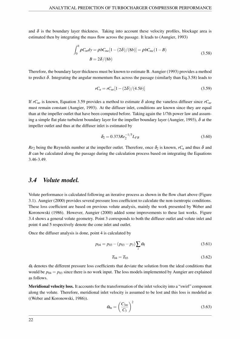
3.4 Volute model.
Volute performance is calculated following an iterative process as shown in the flow chart above (Figure3.1). Aungier (2000) provides several pressure loss coefficient to calculate the non-isentropic conditions.These loss coefficient are based on previous volute analysis, mainly the work presented by Weber andKoronowski (1986). However, Aungier (2000) added some improvements to these last works. Figure3.4 shows a general volute geometry. Point 3 corresponds to both the diffuser outlet and volute inlet andpoint 4 and 5 respectively denote the cone inlet and outlet.
Once the diffuser analysis is done, point 4 is calculated by
p04 = p03− (p03− p3)∑i
ωi (3.61)
T04 = T03 (3.62)
ωi denotes the different pressure loss coefficients that deviate the solution from the ideal conditions thatwould be p04 = p03 since there is no work input. The loss models implemented by Aungier are explainedas follows.
Meridional velocity loss. It accounts for the transformation of the inlet velocity into a “swirl” componentalong the volute. Therefore, meridional inlet velocity is assumed to be lost and this loss is modeled as((Weber and Koronowski, 1986)).
ωm =
(C3m
C3
)2
(3.63)
22

CHAPTER 3. IMPLEMENTATION.
4
3
5
ω
Figure 3.4: Volute geometry.
Tangential velocity loss. Ideal conditions must verify conservation of angular momentum. If angularmomentum decreases across the volute, a tangential velocity loss is implemented that is described as((Weber and Koronowski, 1986)).
ωu = 0.5r3C2
u3
rrC2u4
[1− 1
SP2
](SP≥ 1)
ωu =r3C2
u3
rrC2u4
[1− 1
SP
]2
(SP < 1)(3.64)
being SP the sizing parameter, given by
SP =
(r3Cu3
r4C4
)(3.65)
Skin friction loss. It accounts for the losses caused by the frictional losses and it is described as((Aungier, 2000))
ωs f = 4c f (C4/C3)2L/dh
L = π(r5 + r6)/2
dh =√
4A4/π
(3.66)
L being the average flow path length. Finally, once point 4 is known, outlet cone conditions are computedby ((Aungier, 2000)).
C5A5 =C4A4
p05 = p04− (p03− p3)ωEC
T05 = T04
(3.67)
where ωEC is the exit cone loss described as follows (Aungier, 2000).
23

ANALYTICAL PREDICTION OF TURBOCHARGER COMPRESSOR PERFORMANCE
Exit cone loss.ωEC = [(C4−C5)/C3]2 (3.68)
3.5 CFD losses.
The CFD simulations are run in STAR-CCM+ and they use steady-state RANS calculations, see Sund-strom et al. (2015). Table 3.2 shows the main properties of the numerical setup.
Table 3.2: CFD model properties (Adapted from Kerres et al. (2016)).
Numerical setupDomains Inlet pipe, impeller, vaneless diffuser, volute and outlet pipeGrid type, size Polyhedral + prism layer, 1.1 ·106
Walls Adiabatic, Wall functionTurbulence RANS, SST k−omegaRot.-stat. interf. Mixing planeSolver 2nd order implicit coupledBoundary cond. Inlet: Mass flow
Outlet: Pressure
3.5.1 Impeller losses.
After several decades of research studies, impeller loss mechanisms are not fully understood yet. Thecomplex flow involved and the wide range of different working conditions that may appear (from highlyunsteady conditions as surge to supersonic conditions that leads to choking) make very hard to indepen-dently analyze each internal loss. For example if the flow is supersonic at the impeller inlet, shock wavesmay appear at the same place than the losses caused by the incidence angle and the well-known frictionalloss. Therefore, to independently estimate the impeller losses from the CFD some assumptions need tobe done. Besides, not all the implemented losses in the one-dimensional models have been investigated.The present study is focused on incidence, skin friction, choking, blade-loading and wake-mixing losses.Future works could go further and investigate other losses such as tip clearance losses or recirculationlosses.
The main assumption of this study is to divide the impeller passage into four different parts and relateeach loss to a single part. Though this assumption is clearly reasonable with some losses, it is not veryaccurate to others. For example incidence loss is related to the inlet part, where it must only appear andthus results may not diverge a lot from reality. On the other hand, even blade loading loss is supposedto be more significant after the throat due to the larger pressure gradients, it must also appear before thethroat . However, all assumptions will be motivated.
Figure 3.5 (a) shows how impeller passage is divided into four different parts (A-D) limited by fivedifferent sections (i-v) where the flow properties are measured. Figure 3.5 (b) shows those sections inthe CFD model. Though each part will be explained below in depth, Table 3.3 summarizes where eachone is located and which losses are measured along it.
Harley (2013) measures the total losses along the impeller but as a sum, without distinguishing betweeneach internal loss and external losses. However, this study follows a methodology similar to it, measuringjust the inlet and outlet properties and then calculating the losses as the deviations from the ideal condi-tions. Each loss, either internal or external loss, is described as an entropy rise. Figure 3.6 shows how it
24

CHAPTER 3. IMPLEMENTATION.
Incidence
Blade
Loading
Shock
Jet-Wake
Mixing
i ii
iv
v
iii
(a) Schematic (Courtesy of Kerres et al. (2016)). (b) CFD model.
Figure 3.5: Entropy field function.
Table 3.3: Impeller parts and related losses.
Part Location Related lossesA Impeller inlet - Throat Incidence, skin frictionB Throat ChokingC Throat - Impeller tip Blade loading, skin frictionD After impeller tip Wake mixing
is done. First, points i and o are fully determined from the CFD by computing the mass flow averages oftotal absolute pressure and temperature at the inlet and outlet planes. Point b denotes the conditions theflow would have if external losses were null. To locate it, Euler’s formula is applied. Mass flow averagevalues of rwCu are calculated at the inlet and outlet planes. The difference between both values is thetotal blades work (∆h0b = hb− hi). Assuming that external losses are applied at a constant pressure asdone in the one-dimensional models, the entropy rise associated to the external losses is obtained by thethermodynamic relation
T ds = dh− vd p (3.69)
Since pressure is constant,
∆sext = cp ln(To
Tb) (3.70)
On the other hand, the entropy rise between b and i is caused by the internal losses. Applying relation3.69 from i to b, it leads to
∆sint = cp ln(
Tb
Ti
)−R ln
(pb
pi
)(3.71)
However, internal and external losses in centrifugal compressors and pumps are mainly described as
adiabatic head (enthalpy) loss coefficients (λi =∆hL
02
U22
), where subscript 2 refers to the impeller tip.
25

ANALYTICAL PREDICTION OF TURBOCHARGER COMPRESSOR PERFORMANCE
Δh0b
ΔSint ΔSext
0i
b
0o
p0o
p0i
h
s
h0o
h0b
h0i
Figure 3.6: h-s diagram along an impeller part.
Therefore, these entropy rises are converted into head loss coefficient by
λi =T02∆sint
U22
(3.72)
Figure 3.7 shows the h-s diagram at the impeller tip. Since compressive effects are present in centrifugalcompressor and head loss is not a state point parameter, it would be an error to directly calculate theenthalpy loss coefficient in each part (Aungier, 1995). However the entropy rise must remain unchangedalong the impeller passage. Thus, working with entropy rises is more consistent than working withenthalpy losses. Each part will be deeper explained as follows, motivating why only some losses aremeasured in each part and describing how they are computed.
Part A. It starts at the impeller inlet and ends slightly before the throat. Though several internal lossescould appear along this part (tip clearance, blade-loading, shock waves,..) just incidence and skin frictionlosses have been taken into account. One-dimensional models describes the incidence loss as the largestone. It is reasonable to consider it as the main loss here due to its guessed larger value and since thisloss must only appear in this part, close to the inlet. Skin friction is also measured in part A because itis independently calculated by computing the skin friction factor (c f ) from the CFD and it is thus easilyseparable from the incidence loss.
To calculate the skin friction loss, it is applied the well-known equation to calculate the frictional enthalpylosses (Equation 3.73). The correction factor ( fc) provided by Aungier (Equation 3.6) is included in orderto calculate the equivalent head loss at the impeller tip. Then, the equivalent entropy rise is obtained byEquation 3.74 that is based on the definition of head loss.
∆hA0s f = fc(0.5ρre fV 2
re f )(4c fLA
Dh) (3.73)
26

CHAPTER 3. IMPLEMENTATION.
Δhb
Σ(Δsint) Σ(Δsext)
01
b
02
p02
p01
h
s
h02
h0b
h0i
Δhext
Δhint
Δhs
Figure 3.7: h-s diagram between impeller inlet and outlet.
∆sAs f = ∆hA
0s f /T02 (3.74)
where A denotes part A, LA is the blade length along this part and Dh is the hydraulic diameter that isestimated as the average between the inlet and the throat hydraulic diameters.
Once skin friction loss is known, the entropy rise caused by the incidence loss can be computed asfollows.
∆sinc = ∆sAint −∆sA
s f (3.75)
where ∆sAint is calculated by applying Equation 3.71 to this part
Part B. It is located at the throat, being limited by two planes very close to each other (d=2mm). Dueto the small size of this part, it is reasonable to consider that just choking losses (if choke exists) have asignificant effect in it. However, external losses have been calculated too. ∆sch is calculated by Equation3.71 that leads to
∆sch = cp ln(
T B0b
T0ii
)−R ln
(pB
0bp0ii
)(3.76)
being ii the inlet plane of this part and b the flow conditions just applying the blade work as it wasexplained before (Figure 3.6)
Part C. It extends from the throat until the impeller tip. Skin friction and blade loading are the onlyinternal losses measured in it. Skin friction is measured due to the same reason than in part A: it is easyto calculate independently. Why blade-loading is also related to this part instead of other internal lossesthat may appear, is motivated by:
• One-dimensional results point blade-loading as the second largest loss after incidence loss that hasbeen already measured before.
27

ANALYTICAL PREDICTION OF TURBOCHARGER COMPRESSOR PERFORMANCE
• It is reasonable to say that blade loading may mostly appear along this part since pressure gradientsare higher and the diffusion process after the throat make the boundary layer to grow. Therefore,the two origins of blade-loading losses mostly happen after the throat while other losses may notbe as concentrated in a single region as this loss.
How each loss is computed is similar than in Part A. First, the entropy rise caused by the external lossesand frictional forces are computed and then, blade loading loss is obtained.
Part D. It is related to wake-mixing loss. It starts at the impeller tip, where the jet and wake are clearlyidentified. It ends where the flow can be considered mixed-out. Since it is not at the same point atevery stage point, some approximation needs to be done. Jhonson and Dean (1966) investigate about thejet-wake flow. One of their conclusions was wake disappears in most of the cases at a radius 1.1 timeslarger than the impeller tip radius. Therefore, plane 5 is defined as a cylindrical section with a radiusequal to 1.13 · r2. Figure 3.8 are taken from the CFD and they show the entropy field at sections iv and vat a random stage point. It is seen how at plane 4 (impeller tip) wake is easily identified being an area ofhigher entropy while at plane 5 flow this entropy variation is much lesser. Once part D is fully defined,wake-mixing loss can be calculated. Since there are no blades along part D, work input is null and thusstagnation temperature must be constant. Applying Equation 3.69 to this conditions and assuming thereare no external losses, entropy rise is calculated by
∆smix =−R ln(
pv
piv
)(3.77)
where iv and v respectively denote the inlet and outlet planes of this part.
(a) Section iv (r2) (b) Section v (1.13r2)
Figure 3.8: Entropy field function.
3.5.2 Vaneless diffuser and volute losses.
Both vaneless diffuser and volute are components where there is no work input. Therefore, the stagnationtemperature is constant in them and entropy rise thus can be calculated by applying relation 3.69 that,under these conditions, leads to
∆si =−R ln(
po
pi
)(3.78)
where subscripts i and o denote the inlet and outlet plane of each component.
28

CHAPTER 3. IMPLEMENTATION.
Figure 3.9 shows the planes where properties have been measured. Sections 2 and 3 are the diffuserinlet and outlet sections 3 and 5 are the volute inlet and outlet. Plane 4 has been added in order toindependently study the losses along the volute scroll and volute cone.
Figure 3.9: Vaneless diffuser and volute sections.
29

Chapter 4
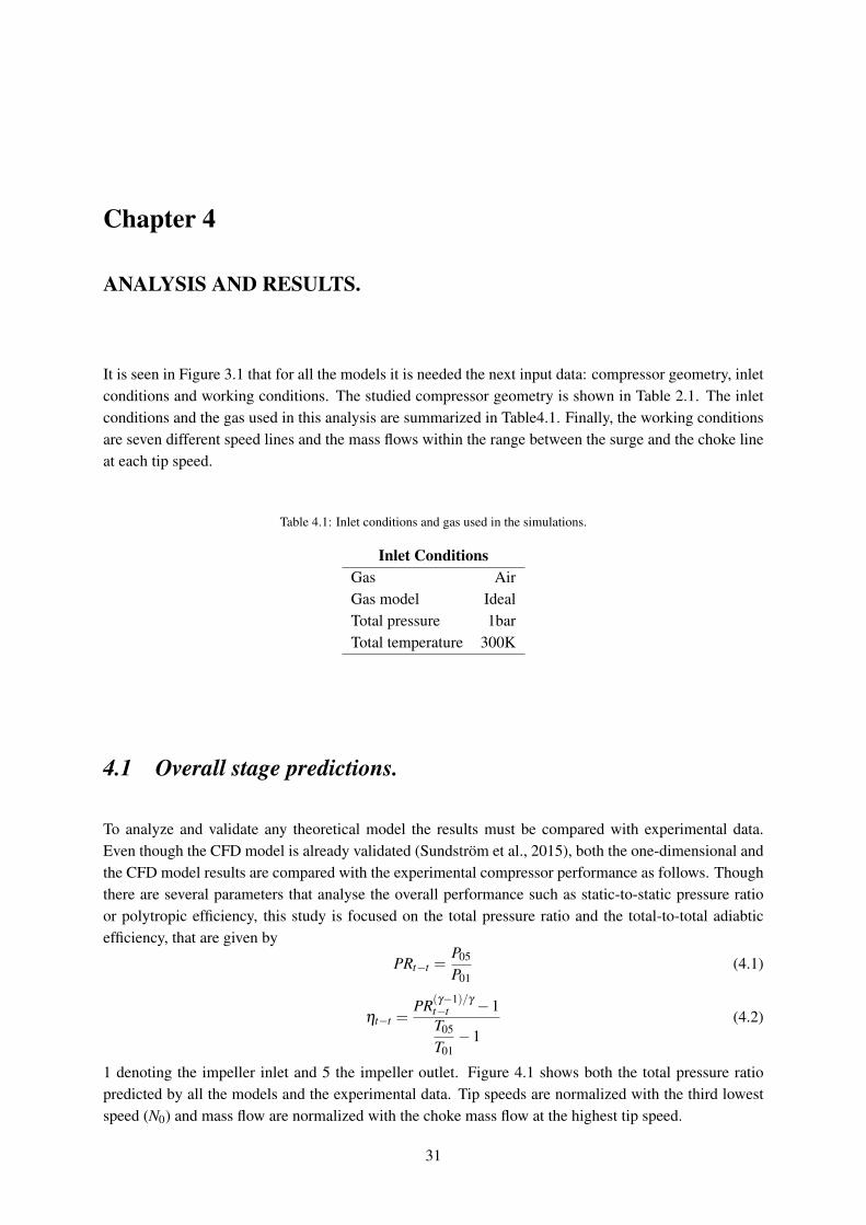
ANALYSIS AND RESULTS.
It is seen in Figure 3.1 that for all the models it is needed the next input data: compressor geometry, inletconditions and working conditions. The studied compressor geometry is shown in Table 2.1. The inletconditions and the gas used in this analysis are summarized in Table4.1. Finally, the working conditionsare seven different speed lines and the mass flows within the range between the surge and the choke lineat each tip speed.
Table 4.1: Inlet conditions and gas used in the simulations.
Inlet ConditionsGas AirGas model IdealTotal pressure 1barTotal temperature 300K
4.1 Overall stage predictions.
To analyze and validate any theoretical model the results must be compared with experimental data.Even though the CFD model is already validated (Sundstrom et al., 2015), both the one-dimensional andthe CFD model results are compared with the experimental compressor performance as follows. Thoughthere are several parameters that analyse the overall performance such as static-to-static pressure ratioor polytropic efficiency, this study is focused on the total pressure ratio and the total-to-total adiabticefficiency, that are given by
PRt−t =P05
P01(4.1)
ηt−t =PR(γ−1)/γ
t−t −1T05
T01−1
(4.2)
1 denoting the impeller inlet and 5 the impeller outlet. Figure 4.1 shows both the total pressure ratiopredicted by all the models and the experimental data. Tip speeds are normalized with the third lowestspeed (N0) and mass flow are normalized with the choke mass flow at the highest tip speed.
31
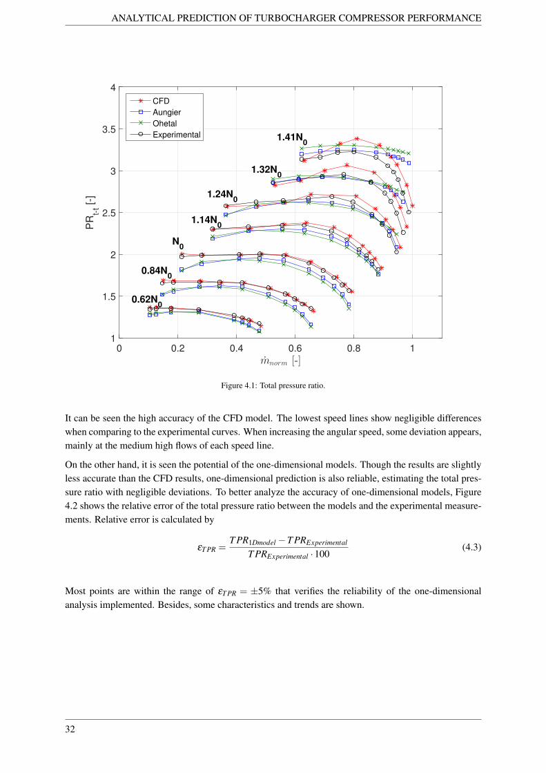
ANALYTICAL PREDICTION OF TURBOCHARGER COMPRESSOR PERFORMANCE
0 0.2 0.4 0.6 0.8 1
mnorm [-]
1
1.5
2
2.5
3
3.5
4P
Rt-
t [-]
CFD
Aungier
Ohetal
Experimental
1.24N0
1.32N0
1.41N0
1.14N0
N0
0.84N0
0.62N0
Figure 4.1: Total pressure ratio.
It can be seen the high accuracy of the CFD model. The lowest speed lines show negligible differenceswhen comparing to the experimental curves. When increasing the angular speed, some deviation appears,mainly at the medium high flows of each speed line.
On the other hand, it is seen the potential of the one-dimensional models. Though the results are slightlyless accurate than the CFD results, one-dimensional prediction is also reliable, estimating the total pres-sure ratio with negligible deviations. To better analyze the accuracy of one-dimensional models, Figure4.2 shows the relative error of the total pressure ratio between the models and the experimental measure-ments. Relative error is calculated by
εT PR =T PR1Dmodel−T PRExperimental
T PRExperimental ·100(4.3)
Most points are within the range of εT PR = ±5% that verifies the reliability of the one-dimensionalanalysis implemented. Besides, some characteristics and trends are shown.
32

CHAPTER 4. ANALYSIS AND RESULTS.
0 0.2 0.4 0.6 0.8 1
Normalized mass flow [-]
-25
-20
-15
-10
-5
0
5
10
15
20
25
30R
ela
tive
TP
R e
rro
r [%
]0.62 N
0
0.84 N0
N0
1.14 N0
1.24 N0
1.32 N0
1.41 N0
(a) Aungier’s losses set.
0 0.2 0.4 0.6 0.8 1
Normalized mass flow [-]
-25
-20
-15
-10
-5
0
5
10
15
20
25
30
Rela
tive T
PR
err
or
[%]
0.62 N0
0.84 N0
N0
1.14 N0
1.24 N0
1.32 N0
1.41 N0
(b) Oh et al.’s losset set.
Figure 4.2: Relative TPR error between experimental measurements and 1D results.
• At the lowest speed lines (0.62N0−N0) both set models results are very similar. An underestima-tion (εT PR < 0$) of the total pressure ratio is shown on those speed lines. Moreover, it can be seenhow this deviation increases towards the surge and the choke side of the map, reaching the highestdeviation (∼−15%) next to the choke line. A minimum close the design points is shown, reachingerror values of −3%.
• The predictions are reached at 1.14N0 and 1.24N0. Deviations are mostly minor than 5%. Under-estimations still predominates.
• At the highest speeds (1.34N0 and 1.41N0), high accuracy is still reached towards the surge line.However, prediction becomes worse towards the choke side of the map. It could be caused by ahigh underestimation of choking losses that leads to higher total pressure ratios. While Aungierprovides a model for this losses, Oh et al.’s set does not even model it. Therefore, it is reasonablethe even worse prediction of Oh et al.’s set. Besides, at the highest speed (1.41N0) both modelsoverestimate (εT PR > 0%) the pressure ratio along the whole line.
Total-to-total adiabatic efficiency is shown in Figure 4.3. The relative error of all the theoretical modelsare plotted too. CFD model results show almost a perfect match again. Only at the lowest speed line,deviations greater than 10% (red dashed lines) are reached. In general, it appears a slight overestimationthat is caused by the assumption of adiabatic walls introduced in the CFD model (Sundstrom et al., 2015)
One-dimensional predictions show larger deviation than the CFD model again. Both models still havesimilar results and an underestimation predominates. At the lowest speed lines (0.62N0−N0), the effi-ciency prediction worsens towards the choke line and error values of 40−50% are reached. On the otherhand, results are overestimated at high speed lines and close to the choke line. It could be caused by awrong choking loss prediction again.
The correct estimation of all the models show the reliability of these theoretical models. However, thereare some deviation trends that can be investigated. In the next sections, several internal and external lossis investigated and the reason of some of the weakest predictions are explained.
33

ANALYTICAL PREDICTION OF TURBOCHARGER COMPRESSOR PERFORMANCE
0 0.5 1
mnorm [-]
0.2
0.4
0.6
0.8
Experim
enta
l
ηt-
t [-]
0.62 N0
0.84 N0
N0
1.14 N0
1.24 N0
1.32 N0
1.41 N0
0 0.5 10.2
0.4
0.6
0.8
Aungie
r
ηt-
t [-]
0 0.5 1-60
-40
-20
0
20
ǫη [%
]
0 0.5 1
mnorm [-]
0.2
0.4
0.6
0.8
Oh e
t al.
ηt-
t [-]
0 0.5 1
mnorm [-]
-60
-40
-20
0
20
ǫη [%
]
0 0.5 10.2
0.4
0.6
0.8
CF
D
ηt-
t [-]
0 0.5 1-60
-40
-20
0
20
ǫη [%
]
Figure 4.3: Total-to-total adiabatic efficiency. Red dashed lines = ±10%
34

CHAPTER 4. ANALYSIS AND RESULTS.
4.2 Impeller performance and losses prediction.
4.2.1 Blades work.
The imparted work from the impeller to the fluid determines the compressor performance and limits theachievable total pressure ratio. Therefore, it is one of the main characteristics that must be investigatedin order to understand the compressor performance. Hence, theoretical models must correctly predict itin order to achieve accurate predictions.
It is reminded that dimensionless blades work coefficient is theoretically described by Euler’s formula as
IB = (U2Cu2−U1Cu1)/U22 (4.4)
and taking into account the slip factor (σ ) and the tip distortion factor (λ dis), one-dimensional modelsdescribe it as
IB = σ(1−λdis
φ2 cotβ2b)−U1Cu1/U22 (4.5)
Figure 4.4 shows the results of IB in all the models.
0 0.2 0.4 0.6 0.8 1
mnorm [-]
0.4
0.45
0.5
0.55
0.6
0.65
0.7
0.75
0.8
0.85
0.9
IB[-]
CFD
Aungier
Ohetal
Figure 4.4: Dimensionless blades work coefficient prediction.
It is seen how both one-dimensional losses set yield almost equal results as it was expected since totalpressure ratios estimated are very similar (Fig. 4.1). However, some differences between CFD andone-dimensional results are evident. Slip factor estimation might be a source of deviations. Wiesner’s(1967)REF! slip factor is used in the one-dimensional models. It is constant since it only depends ongeometry parameters. Figure 4.5 shows this estimated slip factor and the value from the CFD model.Only the results of some speed lines are plotted to make it more readable. At the speeds that are notplotted, slip factor takes similar values and trends.
35

ANALYTICAL PREDICTION OF TURBOCHARGER COMPRESSOR PERFORMANCE
It can be seen how CFD slip factor takes values from 0.82 to 0.97. Therefore, one-dimensional modelsare overestimating the slip effect (σ = 0.81). The same Wiesner model overestimation is shown atSchneider et al. (2015). At the lowest speed lines (0.62N0, 0.84N0 and N0), the IB differences betweenCFD and one-dimensional models are mainly caused by this slip factor variations. Towards the surgeline, slip factor difference is largest and thus IB difference too. There is a minimum difference of σ nextto the design point, being at that point minimum the variation of IB between CFD and one-dimensionalmodels. Towards the choke line, slip factor slightly grows and so does IB.
0 0.2 0.4 0.6 0.8 1
mnorm [-]
0.5
0.6
0.7
0.8
0.9
1
σ[−
]
0.62 N0
N0
1.24 N0
1.41 N0
One-dimensional
Figure 4.5: Slip factor.
However, at the highest speed lines, results are very different. Although CFD slip factor increases to-wards the choke side of the map, showing a sharp growth close to the choke line and Wiesner model stilloverestimates the slip effect, IB is now larger in the one-dimensional analysis than in the CFD model.
4.2.2 Internal losses.
Several internal losses are studied in each theoretical model. Similarly to Table 3.1, Table 4.2 summarizesthe internal losses predicted in each model. Though just five losses are studied in the CFD model, all theother losses should be included in those five in a certain way due to the calculation procedure followed.
Table 4.2: Internal loss mechanisms studied at each model.
Aungier’s set Oh et al.’s set CFD modelIncidence x x x
Skin friction x x xBlade-loading x x xWake-mixing x x x
Clearance x xHub-to-shroud x
Choking x xSupercritical Mach x
Distortion x
36

CHAPTER 4. ANALYSIS AND RESULTS.
Figure 4.6 shows the sum of all the internal losses in each model. Overall, a good match between all themodels is achieved. Specially, between CFD and Aungier model since it can be seen that losses are withinthe same range and they follow the same trend. In those models, along each speed line internal lossesincrease toward the surge and choke line and a minimum appears close to the design point as expecteddue to its higher efficiency. Besides, the increment close to the choke line is higher at the highest speedlines. It is explainable by the fact that choking losses are more significant when the impeller works athigher Mach rotational numbers. On the other hand, though Oh et al. set yields not very different values,it underestimates the losses in relation to the other models. Besides, the increment towards the chokeside of the map does not appear since choking losses are not implemented in this set.
Moreover, taking the CFD as the reference model due to its better overall predictions (Fig. 4.1 and 4.3),Aungier set slightly overestimates the internal losses, mainly at the highest speed lines. Each internalloss is independently investigated as follows.
0 0.2 0.4 0.6 0.8 1
mnorm [-]
0
0.05
0.1
0.15
0.2
0.25
0.3
λimp[-]
CFD
Aungier
Ohetal
Figure 4.6: Internal loss coefficient.
Incidence loss. Figure 4.7 shows the incidence loss coefficient in each model. A good match betweenall the model is again shown, mainly between Aungier and CFD models. Oh et al. gives less weight toincidence loss leading to the lower loss values.
Trend is similar for all the models: decreasing towards the choke side of the map. Since incidencelosses are caused by the flow adjustment to the inlet blade angle, they must follow the same trend thanthe absolute difference between the inlet flow angle (β1) and the blade angle (β1b). This difference iscalled the incidence angle. β1 mainly depends on the inlet conditions, inlet geometry and impeller speed.
37

ANALYTICAL PREDICTION OF TURBOCHARGER COMPRESSOR PERFORMANCE
Therefore, it is expected to take similar values for all the models. Effectively, Figure 4.8 shows β1 andβ1b. It can be seen how β1b−β1 decreases towards the choke line motivating the incidence loss trend.Oh et al. and Aungier models are shown together in one line since β1 takes exactly the same values.
0 0.2 0.4 0.6 0.8 1
mnorm [-]
0
0.05
0.1
0.15
λinc[-]
CFD
Aungier
Ohetal
Figure 4.7: Incidence loss coefficient.
Moreover, CFD incidence loss shows larger values. As it was explained in Chapter 3, other losses thatmay appear in impeller part A could be overestimating incidence losses. Besides, CFD incidence losscoefficients show a slight stabilization close to the choke line. At the highest speed lines, that stabilizationappears but there is a drop after it. Incidence losses should not stabilize until incidence angle was zero,when losses must be null since there is no flow adjustment. Figure 4.8 shows how incidence angle is notclose to zero at any operation point. Therefore, the stabilization must be caused by the growth of someother loss at this side of the map. Due to the fact that this effect happens close to the choke line, chokinglosses are probably the cause. Shock waves does not have to appear at the same point at every operationpoint as it happens in a converging-diverging nozzle (Korpela, 2011). CFD throat region was locatedby analyzing mainly the highest speed and highest mass flow points where shock waves are strongest.Therefore, it is reasonable that at lower speeds and even lower mass flows at a constant speed, shockwaves may start before than what it is considered as throat area and thus the losses produced by them areincluded in the incidence loss coefficient, being the reason of the shown stabilization.
38
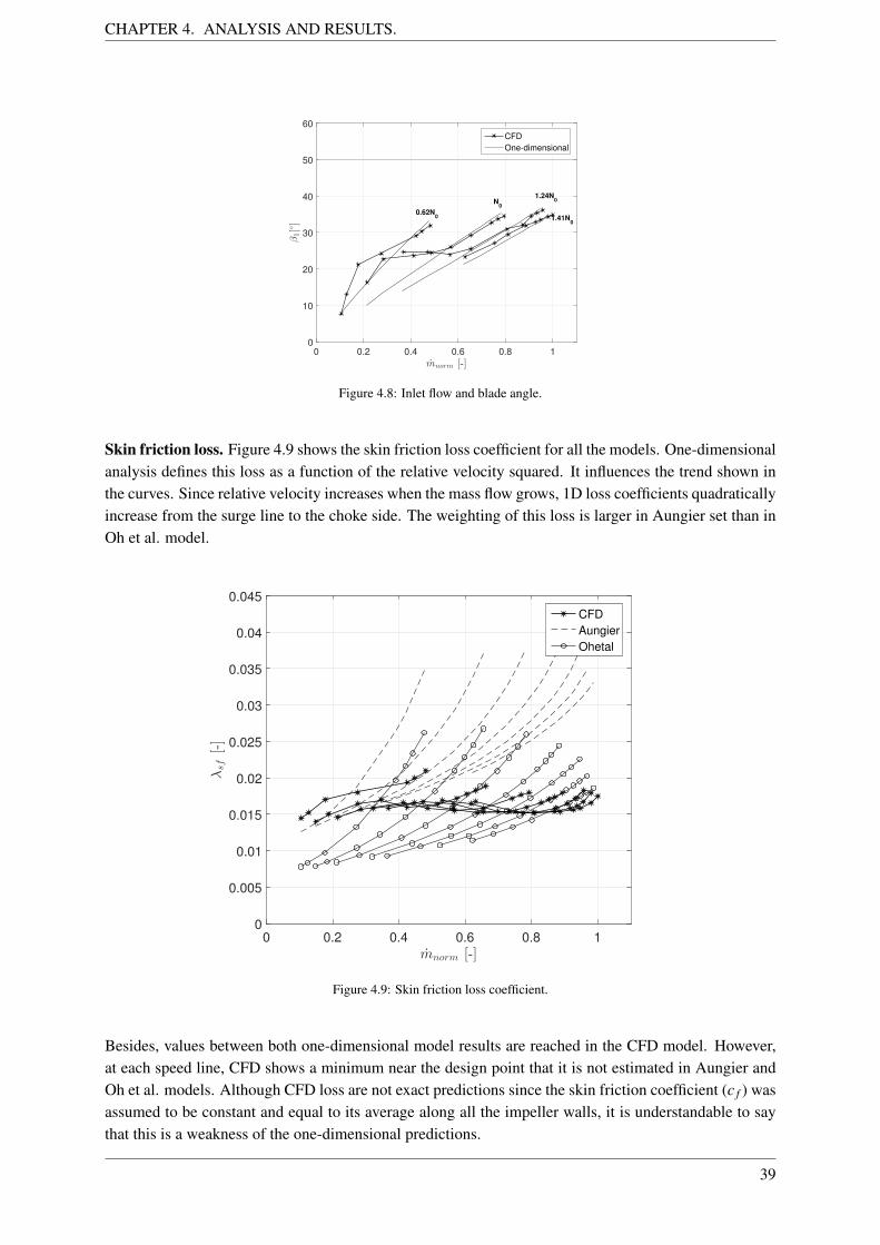
CHAPTER 4. ANALYSIS AND RESULTS.
0 0.2 0.4 0.6 0.8 1
mnorm [-]
0
10
20
30
40
50
60
β1[]
CFD
One-dimensional
0.62N0
N0
1.24N0
1.41N0
Figure 4.8: Inlet flow and blade angle.
Skin friction loss. Figure 4.9 shows the skin friction loss coefficient for all the models. One-dimensionalanalysis defines this loss as a function of the relative velocity squared. It influences the trend shown inthe curves. Since relative velocity increases when the mass flow grows, 1D loss coefficients quadraticallyincrease from the surge line to the choke side. The weighting of this loss is larger in Aungier set than inOh et al. model.
0 0.2 0.4 0.6 0.8 1
mnorm [-]
0
0.005
0.01
0.015
0.02
0.025
0.03
0.035
0.04
0.045
λsf[-]
CFD
Aungier
Ohetal
Figure 4.9: Skin friction loss coefficient.
Besides, values between both one-dimensional model results are reached in the CFD model. However,at each speed line, CFD shows a minimum near the design point that it is not estimated in Aungier andOh et al. models. Although CFD loss are not exact predictions since the skin friction coefficient (c f ) wasassumed to be constant and equal to its average along all the impeller walls, it is understandable to saythat this is a weakness of the one-dimensional predictions.
39

ANALYTICAL PREDICTION OF TURBOCHARGER COMPRESSOR PERFORMANCE
Since the CFD minimum comes from a minimum of c f , one-dimensional results could be refined byimproving the c f estimation.
Blade loading loss. The worst agreement is found in the blade loading losses. Figure 4.10 shows theblade-loading loss coefficient for all the models. Aungier curve is the sum of the blade-loading and thehub-to-shroud loss. Since the cause of both losses are similar, it is understandable to sum them. Besides,hub-to-shroud losses should be included in the CFD blade-loading losses as well, since it includes allthe losses that may appear after the throat except the skin friction loss. Oh et al. set does not model thelosses related to the pressure gradients in the hub-to-shroud direction.
0 0.2 0.4 0.6 0.8 1
mnorm [-]
-0.01
0
0.01
0.02
0.03
0.04
λbl[-]
CFD
Aungier
Ohetal
Figure 4.10: Blade loading loss coefficient.
Between the one-dimensional predictions, it is seen a large difference. Oh et al. losses monotonicallydecrease from the surge line towards the choke line. Aungier losses show a decrement from the surge lineto a point close to the design point where a minimum is found. Then, losses slightly increase towardsthe choke line. Besides, Aungier values are always higher than Oh et al. predictions. The reason ofthis difference is just the addition of the hub-to-shroud losses in the Aungier results. Figure 4.11 showsboth one-dimensional blade loading losses without taking into account the hub-to-shroud losses. It canbe seen how both models would have the same trend, though it is shown that Aungier predicted higherlosses than Oh et al set. The decreasing trend towards the choke line is caused since the diffusion processafter the throat increases when decreasing the mass flow. This leads to higher deceleration of the flowthat causes larger momentum losses since the boundary layer along the blades grows. The reason of thisthicker boundary layer is the higher adverse pressure gradient (Botha and Moolman, 2005).
40

CHAPTER 4. ANALYSIS AND RESULTS.
0 0.2 0.4 0.6 0.8 1
mnorm [-]
0
0.005
0.01
0.015
0.02
0.025
0.03
0.035
0.04λ
bl [
-]
Aungier
Oh et al.
Figure 4.11: Blade loading loss coefficient predicted by the one-dimensional models (without adding hub-to-shroud losses).
On the other hand, CFD losses (Figure 4.10) show a very irregular trend. Besides, even negative valuesare reached at the lowest tip speeds close to the surge line. These unrealistic values may be caused byback flow that alters the values. Later (Figure 4.21) it will be motivated the presence of this back flow. Atthose low speeds, the loss at the design point is similar than the value predicted by the Oh et al. model.However, the trend is the opposite: increasing from the surge line to the choke side of the map. At thehighest speeds the trend is different. From the surge line until close to the design point, losses slightlydecrease. Then, a minimum is reached and finally losses sharply increase towards the choke line. Thistrend is similar than Aungier prediction but with a much higher raise close to the choke line. Thereforesome conclusions arise from all these facts.
• At the lowest speed, CFD losses do not appear to be realistic. Therefore, the trend at the highest tipspeeds may be considered the reference. However, the sharp increment close to the choke line maybe unrealistic as well. It could be produced because some shock waves may appear at the suctionsurface and produce boundary layer separations. This is another source of losses and Aungiermodels it separately.
• Focusing on those regimes, Aungier estimates a similar trend but values are overestimated exceptat the highest mass flow points where shock waves appear to be altering CFD values.
• Since Oh et al. gives very weak predictions, it is seen the importance of modeling the hub-to-shroud losses as well.
41

ANALYTICAL PREDICTION OF TURBOCHARGER COMPRESSOR PERFORMANCE
Mixing loss. The jet-wake flow profile at the impeller tip leads to losses due to the later mixing process.Figure 4.12 shows the mixing loss coefficients predicted by the three models.
0 0.2 0.4 0.6 0.8 1
mnorm [-]
0
0.01
0.02
0.03
0.04
0.05
0.06
λmix[-]
CFD
Aungier
Ohetal
Figure 4.12: Mixing loss coefficient.
Oh et al. model yields the lowest results for this loss. Aungier gives more weight to mixing losses thanOh et al. but the trend it is the same: decreasing from the surge line towards the choke side of the map.On the other hand, though CFD results are similar than Aungier’s towards the surge side of the map,they present a minimum close to the design point. Then, CFD losses increase towards the choke line butwithout reaching as high values as in the surge side. This trend is explainable by taking into account thenext facts.
• Assuming constant wake area ratio (ε), the higher mass flow, the larger wake-mixing losses are(Botha and Moolman, 2005).
• However, it is shown in compressors that the wake area ratio decreases when increasing the massflow (Johnston and Dean, 1966)
To further study this loss, wake area ratio is measured at the impeller tip from the CFD. It is done bystudying the entropy at the impeller tip plane. Wake area must be a high entropy region while jet shouldshow lower values. Figure 4.13 (similar than Figure 3.8) shows this entropy variation from wake tojet. Following the work done by Schneider et al. (2015), wake area ratio is calculated from the CFD byassigning to the wake area the cells where s > s, being s the mass flow entropy average at the plane. Dueto the large entropy gradients between wake and jet, this method becomes not very sensitive to variation
42
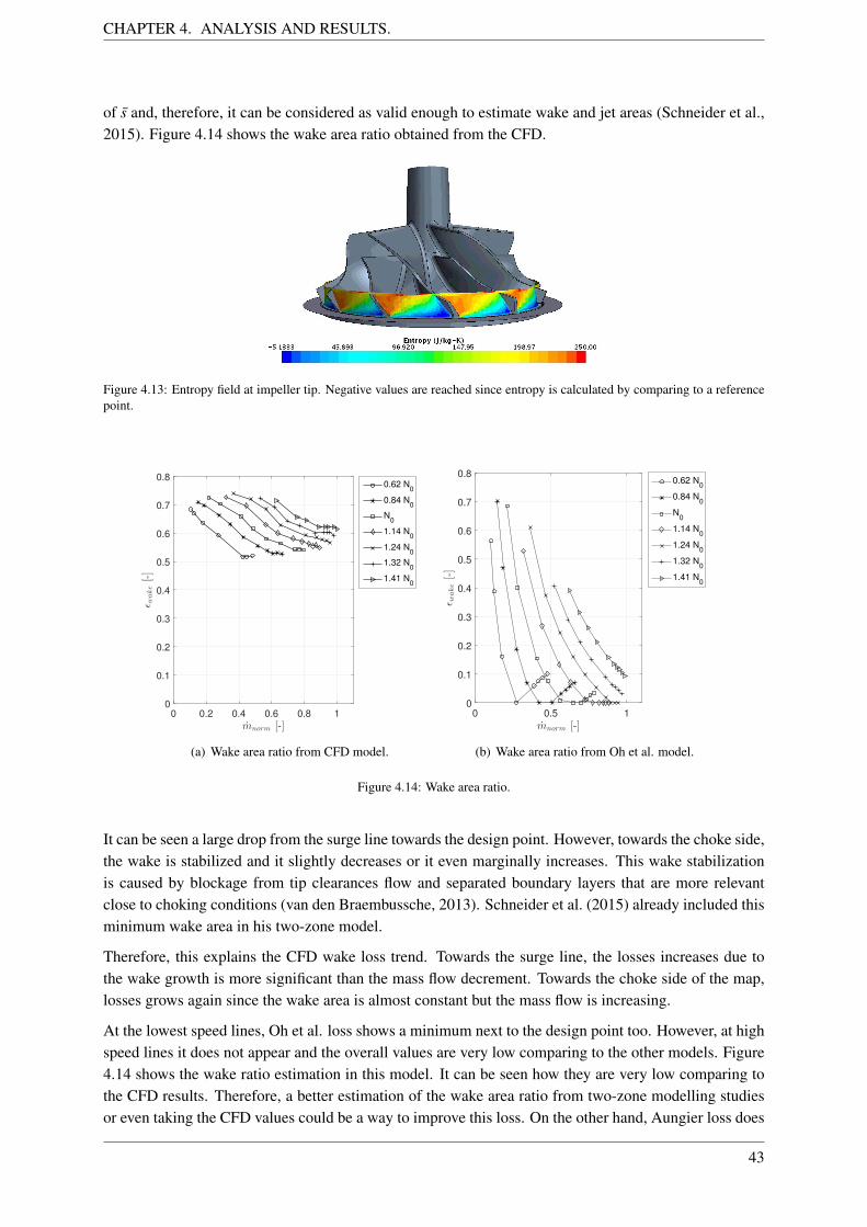
CHAPTER 4. ANALYSIS AND RESULTS.
of s and, therefore, it can be considered as valid enough to estimate wake and jet areas (Schneider et al.,2015). Figure 4.14 shows the wake area ratio obtained from the CFD.
Figure 4.13: Entropy field at impeller tip. Negative values are reached since entropy is calculated by comparing to a referencepoint.
0 0.2 0.4 0.6 0.8 1
mnorm [-]
0
0.1
0.2
0.3
0.4
0.5
0.6
0.7
0.8
ǫwake[-]
0.62 N0
0.84 N0
N0
1.14 N0
1.24 N0
1.32 N0
1.41 N0
(a) Wake area ratio from CFD model.
0 0.5 1
mnorm [-]
0
0.1
0.2
0.3
0.4
0.5
0.6
0.7
0.8
ǫwake[-]
0.62 N0
0.84 N0
N0
1.14 N0
1.24 N0
1.32 N0
1.41 N0
(b) Wake area ratio from Oh et al. model.
Figure 4.14: Wake area ratio.
It can be seen a large drop from the surge line towards the design point. However, towards the choke side,the wake is stabilized and it slightly decreases or it even marginally increases. This wake stabilizationis caused by blockage from tip clearances flow and separated boundary layers that are more relevantclose to choking conditions (van den Braembussche, 2013). Schneider et al. (2015) already included thisminimum wake area in his two-zone model.
Therefore, this explains the CFD wake loss trend. Towards the surge line, the losses increases due tothe wake growth is more significant than the mass flow decrement. Towards the choke side of the map,losses grows again since the wake area is almost constant but the mass flow is increasing.
At the lowest speed lines, Oh et al. loss shows a minimum next to the design point too. However, at highspeed lines it does not appear and the overall values are very low comparing to the other models. Figure4.14 shows the wake ratio estimation in this model. It can be seen how they are very low comparing tothe CFD results. Therefore, a better estimation of the wake area ratio from two-zone modelling studiesor even taking the CFD values could be a way to improve this loss. On the other hand, Aungier loss does
43

ANALYTICAL PREDICTION OF TURBOCHARGER COMPRESSOR PERFORMANCE
not depend on the wake area ratio and that explains why it correctly estimates this loss towards the surgeline comparing to the CFD results but not towards the choke side of the map. Thus, it could be a correctrefinement of this loss to add some dependency of the wake area.
Choking loss. Figure 4.15 shows the losses coefficient related to the shock waves that appear when someportion of the flow reaches supersonic conditions at the throat or close to it. Oh et al. does not model thisloss.
It can be seen that Aungier predicts only shock losses at the highest tip speeds whereas CFD results showlosses at all the tip speeds towards the choke line. At 1.24N0, Aungier reaches values similar to the CFDresults. However, at 1.32N0 and 1.41N0 Aungier predicts lower losses even though the tip speed is larger.It does not appear to be very realistic, since the faster tip speed the larger relative Mach number and thushigher choking losses may be expected.
On the other hand, at the highest tip speeds CFD choking loss increase towards the choke line. However,at lower speeds they present a minimum before the highest mass flow point. It is not expected and itmay be caused because not all the shock is included in the region taken as the throat, as it was explainedbefore (Incidence losses).
0 0.2 0.4 0.6 0.8 1
mnorm [-]
0
0.005
0.01
0.015
0.02
0.025
0.03
0.035
0.04
λch[-]
CFD
Aungier
1.41N0
1.24N0
1.32N0
Figure 4.15: Choking loss coefficient.
44

CHAPTER 4. ANALYSIS AND RESULTS.
Clearance loss. Flow leakage through the clearance between the blades and the shroud causes a lossthat is estimated in both one-dimensional models. Figure 4.16 shows the clearance loss coefficients. Itcan be seen the largest importance that Oh et al. gives to this loss comparing to Aungier. However, thetrend is equal in both models. At the highest tip speeds, loss increases when increasing the mass flow.At lower speeds a maximum appears before the choke line. This maximum moves towards the surge linewhen reducing the tip speed. This trend is explained by Botha and Moolman (2005) as follows.
• Clearance loss increases when the difference between the main flow velocity and the leakage flowvelocity grows. Since the larger mass flow, the larger main velocity is, clearance loss tends toincrease when mass flow grows.
• Besides, clearance loss also increases when the pressure difference over the blades is larger.
First point explains why the larger mass flow, the larger clearance losses are as it is shown at the highesttip speeds. However, after the design point, when increasing the mass flow, pressure ratio decreases.Taking into account the second point, towards the choke line leakage should decrease when increasingthe mass flow. Therefore, when the pressure difference variation is more significant than the incrementin the velocity difference, a maximum appears as it shown at lower tip speeds.
0 0.2 0.4 0.6 0.8 1
mnorm [-]
0
0.005
0.01
0.015
0.02
0.025
0.03
0.035
0.04
0.045
0.05
λcl[-]
Aungier
Oh et al.
Figure 4.16: Tip clearance loss coefficient.
Shock losses. Shock waves may appear in the blade suction at high rotating Mach number and high massflows. These shocks produce losses and boundary layer separations (Aungier, 1995). These losses arenos studied neither in the CFD model nor in the Oh et al. set. Figure 4.17 shows the results given by theAungier model.
45

ANALYTICAL PREDICTION OF TURBOCHARGER COMPRESSOR PERFORMANCE
0 0.2 0.4 0.6 0.8 1
mnorm [-]
0
0.005
0.01
0.015
0.02
0.025
0.03
0.035
0.04
0.045
0.05
λcr[-]
Aungier
Figure 4.17: Shock loss coefficient.
It can be seen that shock losses raises when increasing the tip speed and the mass flow as it was expected.However, it appears that this loss might be overestimated in our compressor. It is in the same orderof magnitude of some other relevant losses such as tip clearance and skin friction losses whereas otherstudies such as Harley et al. (2013) and Schneider et al. (2015)) describe this loss as negligible comparingto the others.
Distortion loss. Only in Aungier model it is studied the loss related to the distorted flow and the mainstream mixing at the impeller tip. Figure 4.18 shows the predicted loss coefficient. Losses increasetowards the choke side of the map. A quadratically trend is shown due to the directly relation betweenthe flow distortion and the skin friction (Aungier, 1995). However, the reached values are negligible,being 10 or 100 times lesser than the other losses.
0 0.2 0.4 0.6 0.8 1
mnorm [-]
0
0.001
0.002
0.003
0.004
0.005
0.006
0.007
0.008
0.009
0.01
λλ[-]
Aungier
Figure 4.18: Distortion loss coefficient.
46

CHAPTER 4. ANALYSIS AND RESULTS.
4.2.3 External losses.
Different types of parasitic works appear in centrifugal compressor. These external losses increase thework input but without raising the flow pressure. As it was explained in Chapter 3, one-dimensionalmodels study three different types of parasitic works: leakage, disk friction and recirculation. On theother hand, external losses are taken from the CFD as a whole.
Figure 4.19 shows the total external losses in all the models and Figure 4.20 shows each external lossestimated by one-dimensional models.
0 0.2 0.4 0.6 0.8 1
mnorm [-]
0
0.05
0.1
0.15
0.2
0.25
0.3
Iext[-]
CFD
Aungier
Ohetal
Figure 4.19: External loss coefficient.
Both one-dimensional models yield similar predictions and their curves are overlapped in Figures 4.19and 4.20. However, they do not match the CFD results. Towards the surge side of the map and speciallyat low tip speeds, one-dimensional analyses highly underestimate the losses. At those operation points,it is expected that recirculation losses predominate over the others. Figure 4.21 shows the back flowmeasured in the CFD at the impeller inlet. It is calculated as a percentage by dividing by the total massflow that goes downstream.
47

ANALYTICAL PREDICTION OF TURBOCHARGER COMPRESSOR PERFORMANCE
0 0.2 0.4 0.6 0.8 1
mnorm [-]
0
0.01
0.02
0.03
0.04
0.05
I L [
-]
Aungier
Oh et al.
(a) Leakage loss coefficient.
0 0.2 0.4 0.6 0.8 1
mnorm [-]
0
0.01
0.02
0.03
0.04
0.05
I R [
-]
Aungier
Oh et al.
(b) Recirculation loss coefficient.
0 0.2 0.4 0.6 0.8 1
mnorm [-]
0
0.01
0.02
0.03
0.04
0.05
I DF [
-]
Aungier
Oh et al.
(c) Disk friction loss coefficient.
Figure 4.20: External losses in one-dimensional models.
It can be seen that the relation between this back flow and the external losses. Therefore, the largestdifference between one-dimensional models and CFD appears to be caused by the high underestimationof the recirculation losses in our compressor.
0 0.2 0.4 0.6 0.8 1
mnorm [-]
0
5
10
15
20
25
30
35
40
mr[%
]
0.62 N0
0.84 N0
N0
1.14 N0
1.24 N0
1.32 N0
1.41 N0
Figure 4.21: Reverse mass flow percentage.
On the other hand, towards the choke side of the map one-dimensional external losses are higher than inthe CFD. It may be caused by an overestimation of the leakage loss since it is by far the most relevantexternal loss in one-dimensional models (Figure 4.20).
48
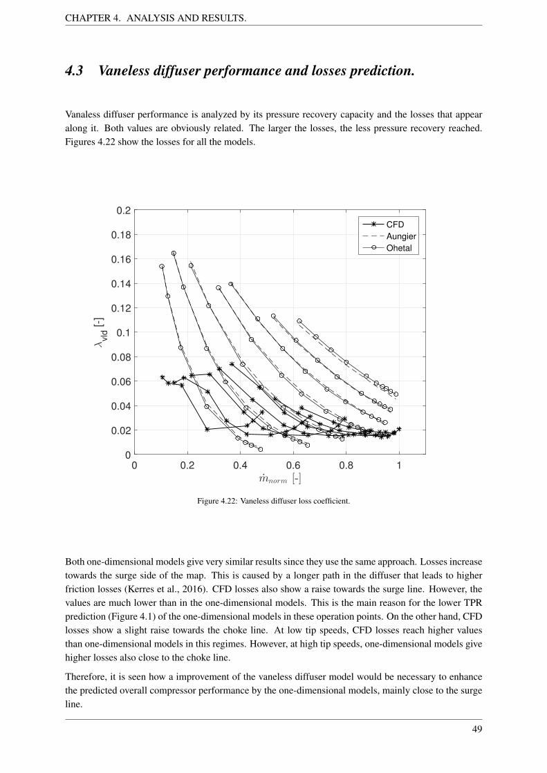
CHAPTER 4. ANALYSIS AND RESULTS.
4.3 Vaneless diffuser performance and losses prediction.
Vanaless diffuser performance is analyzed by its pressure recovery capacity and the losses that appearalong it. Both values are obviously related. The larger the losses, the less pressure recovery reached.Figures 4.22 show the losses for all the models.
0 0.2 0.4 0.6 0.8 1
mnorm [-]
0
0.02
0.04
0.06
0.08
0.1
0.12
0.14
0.16
0.18
0.2
λvld
[-]
CFD
Aungier
Ohetal
Figure 4.22: Vaneless diffuser loss coefficient.
Both one-dimensional models give very similar results since they use the same approach. Losses increasetowards the surge side of the map. This is caused by a longer path in the diffuser that leads to higherfriction losses (Kerres et al., 2016). CFD losses also show a raise towards the surge line. However, thevalues are much lower than in the one-dimensional models. This is the main reason for the lower TPRprediction (Figure 4.1) of the one-dimensional models in these operation points. On the other hand, CFDlosses show a slight raise towards the choke line. At low tip speeds, CFD losses reach higher valuesthan one-dimensional models in this regimes. However, at high tip speeds, one-dimensional models givehigher losses also close to the choke line.
Therefore, it is seen how a improvement of the vaneless diffuser model would be necessary to enhancethe predicted overall compressor performance by the one-dimensional models, mainly close to the surgeline.
49

ANALYTICAL PREDICTION OF TURBOCHARGER COMPRESSOR PERFORMANCE
4.4 Volute performance and losses prediction.
As it was explained in Chapter 3, volute is divided into two parts: volute funnel and volute cone. Figure4.23 and 4.24 show the losses of both parts in all the models. Both one-dimensional models use thesame volute funnel and cone model. Hence, both results are very similar and their curves are almostoverlapped in all the figures.
0 0.2 0.4 0.6 0.8 1
mnorm [-]
0
0.05
0.1
0.15
0.2
0.25
0.3
0.35
λvol−funnel[-]
CFD
Aungier
Oh et al.
Figure 4.23: Volute funnel recovery coefficient.
Volute cone losses are correctly predicted by the one-dimensional models (same trend and very similarvalues in overall) whereas funnel losses are highly overestimated. To better explain these differences,Figure 4.25 show all the estimated losses along the volute funnel model. Pressure loss coefficient areshown instead of λ coefficients. It is reminded that pressure loss coefficients are described as
wi =∆pL
i
p03− p3(4.6)
Skin friction appears to be negligible comparing to the other losses. CFD funnel loss shows a similartrend than tangential velocity loss coefficient. It is shown a minimum that coincide with the ”optimalvolute sizing point”, where the angular momentum is better conserved. Towards the surge line, CFDlosses increase due to diffusion losses and towards the choke line they also raises owing to the meridionalvelocity loss (Kerres et al, 2016). However, even though one-dimensional losses also increase towards thechoke line, their increment is much higher, showing the largest differences at those regimes. Therefore,taking into account Figure 4.25 again, the overestimation of the meridional velocity loss appears to bethe reason of the weak volute funnel prediction.
50

CHAPTER 4. ANALYSIS AND RESULTS.
0 0.2 0.4 0.6 0.8 1
mnorm [-]
0
0.02
0.04
0.06
0.08
0.1
λvol−cone[-]
CFD
Aungier
Oh et al.
Figure 4.24: Volute cone loss coefficient.
0 0.2 0.4 0.6 0.8 1
mnorm [-]
0
0.2
0.4
0.6
0.8
wm
[-]
Aungier
Oh et al.
(a) Meridional velocity loss coefficient.
0 0.2 0.4 0.6 0.8 1
mnorm [-]
0
0.2
0.4
0.6
0.8
wu[-]
Aungier
Oh et al.
(b) Tangential velocity loss coefficient.
0 0.2 0.4 0.6 0.8 1
mnorm [-]
0
0.2
0.4
0.6
0.8
wsf[-]
Aungier
Oh et al.
(c) Skin friction loss coefficient.
Figure 4.25: Pressure loss coefficients in 1D volute funnel models.
51

ANALYTICAL PREDICTION OF TURBOCHARGER COMPRESSOR PERFORMANCE
4.5 Losses breakdown.
A common way to further study all the losses is by breaking down them. Figures 4.26, 4.27 and 4.28show the losses breakdown for the lowest tip speed (U2 = 0.62N0), the medium speed (U2 = 1.14N0) andthe highest one (U2 = 1.41N0). They summarize all the losses studied in the previous sections. However,these graphs give a better understanding of which losses are more relevant at each regime. Besides, it isalso seen the difference between the total work input and the final useful work.
The white area below the coloured areas denotes the useful work, i.e. the work that is fully used toincrease the fluid pressure. Then, each coloured area shows the loss produced by each different source.Finally, the upper line (above External Losses in the CFD graphs or Leakage in the one-dimensionalmodels) denotes the total work consumed by the compressor. Moreover, the blades work is also visibleas the area below the last external loss. The losses that are negligible at each model, such as recirculationor distortion losses, are not discernible and therefore they are not pointed.
Even though all the losses have been already explained, some conclusion are extracted from these plots.
• Overall, most relevant losses are the external, incidence, vaneless diffuser and volute losses. Be-sides, largest differences between CFD and one-dimensional models are found in the externallosses, vaneless diffuser and volute.
• At low tip speeds, external losses show a sharp increase towards the surge large due to the backflow. This increment is not predicted by the one-dimensional models. This is the reason why atlow tip speeds and close to the surge line the work input calculated by the CFD is much largerthan the predicted by the one-dimensional models. However, efficiency is similar at those regimes(Figure 4.3). This is caused by a lower useful work in the one-dimensional models. The highoverestimation of the vaneless diffuser loss is the main reason of it.
At higher tip speeds, external losses and work input become more similar in all the models, beingeven higher in the one-dimensional models at the highest tip speed.
• Incidence loss is the largest impeller loss. As it was seen in Figure 4.7, it follows the same trendin all the models but being higher in the CFD. The weight of this loss slightly decreases whenworking at higher tip speeds.
• The total pressure ratio reached is defined by the area below the last impeller loss. This is inagreement with Figure 4.1. At low tip speeds, one-dimensional models underestimate this areagiving lower total pressure ratios but at the highest tip speed it is the opposite.
• Largest differences are found in the vaneless diffuser. Close to the surge large, it is the highest losspredicted by the one-dimensional losses at all the tip speeds. However, it is not the most relevantloss in the CFD model. It is even almost negligible at the highest tip speeds.
• Volute losses are in big disagreement between the models. Towards the surge line, it is similar inall the models at every speed. However, when increasing the mass flow at low tip speeds, one-dimensional models predict a sharply increment that leads to become this loss in the most relevant.CFD also shows a loss increment but much lower. At higher tip speeds, this increment is not assharp as before and volute losses are more similar between all the models.
52

CHAPTER 4. ANALYSIS AND RESULTS.
0.2 0.3 0.4
mnorm [-]
0
0.2
0.4
0.6
0.8
1λ
[-]
Volute
Diffuser Skin friction
Choking
Mixing
Blade Loading
Incidence
External Losses
(a) CFD.
0.2 0.3 0.4
mnorm [-]
0
0.2
0.4
0.6
0.8
1
λ [-]
Volute
Diffuser
Skin friction
Clearance
Blade Loading
IncidenceMixing
Disk friction
Leakage
(b) Aungier.
0.2 0.3 0.4
mnorm [-]
0
0.2
0.4
0.6
0.8
1
λ [
-]
Leakage
Volute
Diffuser
Clearance
Skin friction
Incidence
Blade Loading
Disk friction
Mixing
(c) Oh et al.
Figure 4.26: Losses breakdown (U2 = 0.62N0).
0.4 0.5 0.6 0.7 0.8
mnorm [-]
0
0.2
0.4
0.6
0.8
1
λ [-]
Volute
DiffuserSkin friction
Choking
Blade Loading
Mixing
Incidence
External Losses
(a) CFD.
0.4 0.5 0.6 0.7 0.8
mnorm [-]
0
0.2
0.4
0.6
0.8
1
λ [
-]
Mixing
Leakage
Blade Loading
Incidence
Disk friction
Skin friction
Clearance
Diffuser
Volute
Shock
Choking
(b) Aungier.
0.4 0.5 0.6 0.7 0.8
mnorm [-]
0
0.2
0.4
0.6
0.8
1
λ [-]
Volute
Leakage
Incidence
Blade Loading
Clearance
Skin frictionDiffuser
Mixing
Disk friction
(c) Oh et al.
Figure 4.27: Losses breakdown (U2 = 1.14N0).
0.7 0.8 0.9 1
mnorm [-]
0
0.2
0.4
0.6
0.8
1
λ [-]
External Losses
Incidence
Volute
ChokingSkin friction
Diffuser
Blade Loading
Mixing
(a) CFD.
0.7 0.8 0.9
mnorm [-]
0
0.2
0.4
0.6
0.8
1
λ [
-]
Volute
Diffuser
ClearanceShock
Skin friction
Blade LoadingIncidence
Disk friction
Leakage
Mixing
(b) Aungier.
0.7 0.8 0.9
mnorm [-]
0
0.2
0.4
0.6
0.8
1
λ [
-]
Volute
Skin friction
Clearance
Diffuser
Mixing
Blade LoadingDisk friction
Leakage
Incidence
(c) Oh et al.
Figure 4.28: Losses breakdown (U2 = 1.41N0).
53


Chapter 5
CONCLUSIONS AND FUTURE WORK.
5.1 Conclusions.
Centrifugal compressors are still a engineering challenge due to the complexity of the flow and thephenomena involved. Numerical solutions carried out in CFD software give very accurate performancepredictions, at least in a very wide range of regimes. However, this accuracy requires very complexmodels, long computation times and expensive hardware. In this thesis, it has been seen the potential ofthe much simpler analytical approaches to predict a turbocharger compressor performance. Specifically,two different one-dimensional models have been successfully implemented. They are based on the workdone by Aungier (2000) and Oh et al. (1997). Needing much less geometric input data and much shortercomputational times (∼ 60 seconds to calculate 77 operation points running in a 4 cores processor) thanCFD calculations, they correctly estimate the compressor performance prediction:
• Comparing with the compressor experimental measurements, the implemented one dimensionalmodels estimate the total pressure ratio with an absolute relative error less than 5% in 49 and 41operation points respectively of a total of 77 calculated regimes. Expanding the range, 69 and 61points are predicted with an absolute relative error less than 10%. The weakest total pressure ratioestimations are shown at the highest speed lines and close to the choke line, reaching a maximumrelative error of ∼ 25% in both models.
• Regarding the total-to-total adiabatic efficiency, Aungier model predicts 42 and 60 points withan absolute relative error less than 5% and 10% respectively, whereas Oh et al. model estimates40 and 55 points within those error ranges. The highest errors are reached at low tip speeds andtowards the choke line, taking a maximum value of 60%.
Hereafter, to better understand the advantages and weaknesses of our one-dimensional analysis, theresults were compared to numerical RANS simulations of the same compressor. Several losses weremeasured from the CFD by their entropy raise. The CFD impeller region was divided into four differentparts to measure the incidence, choking, blade-loading, mixing and blade-loading losses. The vanelessdiffuser and volute losses were directly calculated measuring the entropy rise between the inlet and theoutlet of each component. Some conclusions are taken from this analysis.
• Overall, the sum of the impeller internal losses is well predicted, specially by the Aungier model.It gives the same trend along the whole map but a slight losses overestimation is shown. Withinthe internal losses measured in the CFD, incidence losses appear to be the most significant lossesand, at the same time, they are the best predicted losses by the one-dimensional analysis. Skinfriction is also correctly estimated by the models. On the other hand, blade-loading losses shows abig disagreement between CFD and one-dimensional analysis. Choking and mixing losses do not
55

ANALYTICAL PREDICTION OF TURBOCHARGER COMPRESSOR PERFORMANCE
disagree as much as blade-loading losses do, but they differ either in trend or in magnitude at someregimes.
It is reminded that not all the impeller internal losses that are modeled in the one-dimensionalanalysis were measured in the CFD.
• External losses match at high tip speeds. However, at low tip speed and close to the surge line CFDlosses sharply increase that appears to be related to the back flow. This increment is not predictedby the one-dimensional models, giving an almost constant value along each speed line.
• The stationary components (vaneless diffuser and volute) show the largest differences between theone-dimensional analysis and CFD results. Vaneless diffuser is highly overestimated, speciallyclose to the choke line at every regime. On the other hand, though the volute cone losses are verysimilar between CFD and one-dimensional models, the losses along the volute funnel show a largedifference at low speeds and close to the choke line. It appears to be caused by a wrong predictionof the meridional losses. Therefore, both components have a lot of influence in the weakest overallpredictions.
Seeing these results, one-dimensional model can be considered a helpful and useful tool to investigate anddesign centrifugal compressor, specially in the early design stages. Low total pressure ratio and efficiencyerrors can be expected. Thereafter, CFD models allow to further understand all the phenomena, betterpredict the performance and test different three-dimensional geometries.
Finally, it has been seen how to compare ”loss by loss” CFD results with one-dimensional models gives afurther knowledge of the one-dimensional analysis. Even though CFD losses are very hard to be indepen-dently measured and some improvements are needed, it is a good methodology to detect the weaknessesof one-dimensional losses correlations and improve them without needing expensive experimental tests.
5.2 Future work.
Several future work could be carried out to go further in this kind of investigation. First, regarding theone-dimensional analysis, not all the components that can appear in a centrifugal compressor have beenimplemented (e.g. vaned diffusers or return channels). Aungier (2000) provides similar models than theones implemented in this thesis to some of those components. To take advantage of the high flexibilityand modularity that characterises these kind of analysis, all the components should be modeled. Then, awider range of compressor could be analysed with the same code, adding all the components that appearin the real compressor setup and connecting them in the correct order.
Besides, to even cover a wider range of centrifugal compressors, it would be a good practice to implementlosses set that yields well predictions when reaching total pressure ratios higher than∼ 4.2. Both Aungierand Oh et al. losses set are more focused on turbocharger compressor, where lower pressure ratios arereached.
The losses comparison between numerical solution and one-dimensional models yields more possiblefuture work. On one hand, it has been seen how the CFD impeller internal losses are measured in a waythat still shows some weaknesses. Therefore, some improvements could be carried out in that field suchas to measure more losses (e.g. tip clearance or shock losses) or to improve the measurement of somelosses that have been already investigated (e.g. a better location of the throat area).
On the other hand, the numerical and analytical comparison has also shown some one-dimensional pre-diction weaknesses. Specially, in the stationary components performance. The CFD losses of those
56
CHAPTER 5. CONCLUSIONS AND FUTURE WORK.
components can be considered trustworthy since no assumptions were done and the compressor perfor-mance is predicted with high accuracy at almost all the speed lines. Taking this results as the reference,it is seen a high deviation of the one-dimensional results. Therefore, future work could improve thosestationary component models. Several analytical models can be found in the literature e.g. the volutemodel carried out by van den Braembussche et al. (1999). Finally, some weaknesses in the impellerinternal losses correlations have been revealed such as a slip factor overestimation and the need of abetter mixing loss model that depends on the wake ratio. Therefore, future work can also be focused onenhance the impeller internal losses implemented.
57


Appendix A
RESUMEN EN ESPANOL DEL TRABAJO.
A.1 Introduccion y objetivos.
A.1.1 Introduccion y marco de referencia.
Desde hace varios anos, la tendencia de downsizing ha adquirido una gran relevancia en el campo delos motores de combustion interna alternativos. El efecto mas claro de esta tendencia es ver como losmotores de seis cilindros estan reemplazando a los de ocho, los de seis a su vez estan siendo sustituidospor los de cuatro y, muy recientemente, los motores de tres cilındricos estan desbancando a los de cuatro(Squatriglia, 2016).
El objetivo de esta tendencia es reducir la cilindrada del motor pero manteniendo la misma su potencia,o incluso aumentandola. Esta reduccion de tamano va acompanada de un aumento de eficiencia debido,entre otros factores, a las menores perdidas termicas y de friccion. Con este aumento de eficienia, el mo-tor reduce sus emisiones contaminantes, un factor de crucial importancia para mejorar la sostenibilidady poder cumplir con las presentes normativas que establecen los maximos de contaminacion posibles decualquier motor comercial. Entre las tecnologıas mas implantadas para cumplir con el downsizing seencuentran la sobrealimentacion del motor, la inyeccion directa o la distribucion de valvulas variable.
El presente estudio entra en el campo de la sobrealimentacion. La sobrealimentacion consiste en intro-ducir mas masa de aire en el cilindro durante la etapa de admision, y con ello aumentar la potencia atraves de la combustion de mas aire y combustible. Para aumentar la masa de aire, la sobrealimentacionse basa en aumentar su densidad de entrada. Ese es el objetivo del turbocompresor.
El turbocompresor esta formado por una turbina radial y un compresor centrıfugo que giran en torno aun eje comun. En la Figura A.1 se pueden ver estos componentes. Para conseguir aumentar la densidaddel aire de entrada al motor, los gases de escape son conducidos a la entrada de la turbina. La turbina esimpulsada por estos gases gracias a la gran energıa, principalmente termica, que aun tienen. Por tanto,la turbina trasmite la potencia al eje comun. El rotor del compresor recoge dicha potencia y la utilizapara comprimir el aire atmosferico. A la salida del compresor, el aire posee mayor presion y mayordensidad. A traves de la canalizacion necesaria, este aire presurizado es conducido a la entrada delcilindro, consiguiendo el objetivo deseado.
El presente trabajo se centra en el estudio analıtico del compresor, por ello solo este componente esanalizado a continuacion. El compresor centrıfugo esta compuesto por tres componentes principales:el rotor, el difusor y la voluta. En la Figura A.2 se muestra un esquema de su geometrıa. El rotor,impulsado por el eje, es la unica parte movil del compresor y esta compuesto por una serie de alabes.El aire es conducido a traves de ellos, aumentando su presion gracias al trabajo que estos imparten. Al
59

ANALYTICAL PREDICTION OF TURBOCHARGER COMPRESSOR PERFORMANCE
TURBINA
COMPRESOR
CENTRÍFUGO
EJE COMÚN
Figure A.1: Turbocompresor (Adaptado de NASA).
salir del rotor, el aire fluye a traves del difusor, donde aumenta mas aun su presion gracias a un procesode difusion. El difusor puede tener alabes o no. Finalmente, el aire cruza la voluta, aumentando massu presion. Ademas, la voluta dirige al aire para que tenga una direccion de salida compatible con elelemento al que este conectado a continuacion.
ω
ω
VOLUTA
DIFUSOR SIN
ÁLABES
SALIDA
CÓNICA DE
LA VOLUTA
VOLUTA
CUBO DEL
ROTOR
CONDUCTO
ENTRE
ÁLABES
CARCASA
DEL ROTOR
ÁLABE DEL
ROTOR
Figure A.2: Geometrıa de un compresor centrıfugo.
Durante el diseno de un compresor centrıfugo, es importante la obtencion de modelos matematicos quepuedan predecir su funcionamiento, y ası poder reducir el numero necesario de costosos prototipos ylargos ensayos. A dıa de hoy, mediante soluciones numericas realizadas a traves de modelos de Com-putational Fluid Dynamics (CFD) se pueden obtener precisas simulaciones del compresor centrıfugo.Sin embargo, debido a su gran complejidad, estos modelos requieren largos tiempos de computaciony costoso hardware. Por ello, gracias a la investigacion realizada durante las ultimas decadas, se handesarrollado diferentes modelos unidimensionales (1D) que predicen todo el mapa de funcionamientodel compresor en tiempos muy cortos. Ademas, estos modelos 1D requieren relativamente pocos datosacerca de la geometrıa del compresor. Todo ello los convierte en una potente y util herramienta duranteel proceso de diseno de compresores centrıfugos, principalmente en sus primeras fases.
Varios autores (Harley et al. (2013), Schneider et al. (2015) y Kerres et al. (2016)), clasifican los modelos1D en tres categorıas dependiendo de las zonas de flujo estudiadas: a) modelos cero onas, b) modelos deuna zona y c) modelos de dos zonas.
60
APPENDIX A. RESUMEN EN ESPANOL DEL TRABAJO.
Los modelos cero zonas solo requieren los coeficientes adimensionales de flujo, trabajo y el numeroMach del alabe en el punto de diseno. Estos coeficientes se comparan con los de otro compresor del cualtodo su mapa de funcionamiento sea conocido. Bajo la hipotesis de que los compresores fabricados parael mismo objetivo tienen diseno y rendimiento similar, obtienen el mapa adimensional del compresormediante la extrapolacion del resto de puntos a partir del mapa conocido del compresor de referencia yla proporcion entre sus coeficientes en el punto de diseno. El modelo realizado por Casey and Fesich(2010) es un ejemplo de este tipo de analisis.
Los modelos de una zona alcanzan un mayor nivel de detalle. Asumen el flujo uniforme en cada secciondel compresor. Bajo esta hipotesis, se aplican las ecuaciones de conservacion de masa, momento yenergıa al flujo a traves de cada componente del compresor. Ademas, para obtener las condicionesreales, se aplican diferentes correlaciones empıricas de perdidas. Ejemplos de estos modelos y diferentesconjuntos de correlaciones se pueden encontrar en los trabajos de Galvas (1974), Oh et al. (1997) o(Aungier, 2000).
Finalmente, los modelos de dos zonas se centran en el perfil de flujo central y estela caracterıstico dela salida del rotor. El flujo central, situado junto a la superficie de presion de cada alabe, posee mayorvelocidad y menor entropıa. Por ello, estos modelos lo asumen como flujo sin perdidas. Todas lasperdidas se concentran en la estela, que se encuentra junto a las superficies de succion y posee mayorentropıa que el flujo central. Bajo estas hipotesis, los modelos de dos zonas aplican las ecuaciones deconservacion a cada parte del flujo por separado. Ademas, en el calculo de las condiciones de la estelase aplican diferentes correlaciones de perdidas provenientes de los modelos de una zona. Ejemplos deestos modelos son los analisis realizados por (Oh et al., 2001) y Schneider et al. (2015).
Debido a que los modelos de una zona han sido los mas desarrollados hasta hoy, son los implementa-dos en este trabajo. En concreto, se han desarrollado dos modelos diferentes basados en los trabajos deAungier (2000) y Oh et al. (1997). La razon de esta eleccion es que (Aungier, 2000) proporciona uncompleto analisis en el que todos los componentes del compresor son modelados, incluyendo diferentescorrelaciones de perdidas para cada uno de ellos. Por otro lado, (Oh et al., 1997) realiza una amplia com-paracion entre diferentes correlaciones de perdidas del rotor, entre las que se encuentran correlacionesde muchos otros autores, proporcionando un conjunto optimo de modelos de perdidas.
A.1.2 Objetivos.
Los objetivos del presente trabajo son:
• Implementacion de dos modelos 1D de prediccion del rendimiento de un compresor centrıfugo.
• Analisis de los resultados mediante la comparacion con datos experimentales del mismo compre-sor. En concreto, se estudiara el error relativo en las estimaciones del ratio de presion y la eficienciaadiabatica del compresor.
• Comparacion de las perdidas obtenidas con los resultados obtenidos por simulaciones numericasbasadas en las ecuaciones de Reynolds-averaged Navier–Stokes (RANS) del mismo compresor.Estas simulaciones ya han sido realizadas y, por tanto, el desarrollo del modelo CFD no entra entrelas tareas de este proyecto. Sin embargo, sı que entra como parte de este estudio la busqueda deun metodo para extraer cada perdida individual del modelo CFD y la obtencion y analisis de estosresultados.
61

ANALYTICAL PREDICTION OF TURBOCHARGER COMPRESSOR PERFORMANCE
A.2 Implementacion.
En esta seccion se explican los principales aspectos de los modelos unidimensionales implementados asıcomo la metodologıa seguida para calcular las perdidas en el modelo CFD. En la Tabla A.1 se recogenlos datos geometricos mas relevantes del compresor modelado, ası como las condiciones de entrada delaire y el modelo de gas utilizado.
Table A.1: Datos geometricos compresor, modelo CFD y condiciones de entrada.
Geometrıa del compresor.Diametro exterior del rotor 52.5mmNumero de alabes completos 6Numero de alabes divisores 6Ratio de area de difusion AR=0.708Coeficiente de flujo masico φ dc=0.094Coeficiente de trabajo ϕdc=0.622Numero Mach del alabe Mdc
2 =1.09Propiedades del modelo numerico
Dominios Tuberıa de entrada, rotor, difusor, voluta y tuberıa de salidaTipo de mallado, tamano Poliedrico + capa prismas, 1.1 ·106
Paredes AdiabaticasTurbulencia RANS, SST k−omegaRot.-stat. interf. Plano de mezclaSolver 2nd order implicit coupledCond. contorno. Entrada:Flujo masico
Salida: PresionCondiciones de entrada.
Gas AireModelo de gas IdealPresion total 1barTemperatura total 300K
A.2.1 Modelos unidimensionales.
Los modelos analıticos han sido implementados en MATLAB c©. Siguiendo la modularidad que caracter-iza a los modelos 1D de una zona, cada componente es modelado por separado y luego son conectadosen serie segun el orden en el que aparezcan en el compresor real analizado. Como se dijo anteriormente,a lo largo de cada componente se aplican las ecuaciones de conservacion de masa, momento y energıay las diferentes correlaciones de perdidas. En el rotor, se aplica ademas la conservacion de rotalpıa paracalcular el trabajo de entrada. Debido al caracter empırico de los modelos de perdidas, estos dependen delas condiciones de salida que en un primer momento son desconocidas. Por lo tanto es necesario llevar acabo un calculo iterativo. En la Figura A.3 se presenta el algoritmo de calculo implementado.
62

APPENDIX A. RESUMEN EN ESPANOL DEL TRABAJO.
Geometría
Condiciones de entrada
Condiciones de trabajo
Choque?
Cálculo perdidas externas
FIN
FIN
FIN
No
Sí
Sí
No
RotorNo rotor
Cálculo de condiciones
absolutas y relativas de
entrada.
Cálculo de condiciones
ideales relativas de saluda
(Modelo de Aungier).
Asumir velocidad meridional
o coeficiente de flujo de salida
Cálculo trabajo de álabes
y pérdidas internas
Cálculo condiciones
absolutas de salida
Balance de flujo
másico de salida?
Acualizar velocidad
meridional o coefi-
ciente de flujo de
salida
Cálculo condiciones
absolutas de salida
Figure A.3: Algoritmo de calculo en cada componente.
Aunque el difusor tambien puede ser calculado siguiendo este metodo, Aungier (2000) proporcionaun camino alternativo basado en las ecuaciones de conservacion en su forma diferencial, que a su vezincluyen varios terminos para modelar las diferentes perdidas. Estas ecuaciones se aplican a lo largo delcompresor, resolviendolas mediante metodos numericos.
En la Tabla A.2 se recogen todas las perdidas analizadas en cada componente, ası como una brevedescripcion de su origen. Tambien, se indica entre los dos modelos implementados cual tiene en cuentacada perdida y cual no la modela. Los modelos del difusor y de la voluta son los mismos en ambosanalisis ya que Oh et al. (1997) solo proporciona el analisis del rotor. Por tanto, ambos componentes sonanalizados siguiendo el metodo de Aungier (2000).
Todas las correlaciones de las perdidas se pueden encontrar en el Capıtulo 3. Cabe destacar que Aungier(2000) proporciona las perdida en forma de coeficientes de perdida de presion, mientras que en lacoleccion de Oh et al. (1997) son descritas como perdidas de entalpıa medidas a la salida del rotor.Para hacer un estudio consistente y debido a que en la literatura es mas comun que las perdidas se de-scriban como decrementos de entalpıa, las perdidas de ambos modelos son convertidas en coeficientesadimensionales de perdida de entalpıa (λi), calculados con la siguiente formula.
λi =∆hL
0i
U22
(A.1)
A.2.2 Calculo de perdidas en el modelo CFD.
Para investigar mas a fondo los modelos de perdidas unidimensionales, se comparan las perdidas con lasdel modelo CFD. Sin embargo, es imposible hacer una comparacion de todas las perdidas internas porseparado, ya que en el modelo CFD es imposible valorar todas ellas independientemente debido a quemuchas de ellas actuan simultaneamente y en la misma zona del flujo.
Por ello, primero se comparan las suma de perdidas a lo largo de cada componente, lo que sı que es
63

ANALYTICAL PREDICTION OF TURBOCHARGER COMPRESSOR PERFORMANCE
Table A.2: Perdidas implementadas en cada componente del compresor.
Perdida Aungier Oh et al. OrigenROTOR
Incidencia x xDiferencia entre el angulo de entrada del alabe y del
flujo.Friccion x x Friccion entre el fluido y las paredes.
Holgura x xFlujo que fluye por la holgura entre los alabes y la
carcasa.
Mezcla x xMezcla entre la region central del flujo y la estela a
la salida del rotor.
Perfil x xCrecicimento de la capa lımite a lo largo del alabe y
gradiente de presion en la direccion de alabe aalabe.
Choque x Condiciones de choque alcanzadas en la gargantaNumeroMach su-percrıtico
xOndas de choque locales en la superficie de succiondel alabe que generan separaciones de la capa lımite
Distorsion xDistorsion del flujo a la salida por efectos viscosos
o bloqueosHub-to-shroud
xGrandiente de presion en la direccion del cubo
hacia la carcasa
Externas x xPerdidas externas que incluyen perdidas por fugas,
recirculacion o friccion del discoDIFUSOR
Friccion x x Friccion entre el fluido y las paredes.Difusion x x Perdidas asociadas al proceso de difusion.Curvatura x x Curvatura del difusor.
VOLUTAFriccion x x Friccion entre el fluido y las paredes.
Velocidadmeridional
x xPerdida de la componente meridional de la
velocidad debido a la trayectoria en remolino queadquiere el flujo en la voluta.
Velocidadtangencial
x x Perdida de momento angular.
Salidaconica
x xCambio de una trayectoria en remolino propia de lavoluta a una trayectoria lineal a lo largo del cono.
64

APPENDIX A. RESUMEN EN ESPANOL DEL TRABAJO.
facilmente calculable. Para ello se mide el incremento de entropıa a lo largo de cada componente me-diante el calculo del mass flow average de la temperatura total y presion total tanto a la entrada comosalida de cada componente. Posteriormente, se aplica la siguiente relacion termodinamica de Gibbs paracalcular el incremento de entalpıa.
T ds = dh− vd p ⇒ ∆si = cp ln(
T0o
T0i
)−R ln
(p0o
p0i
)(A.2)
significando los subındices i y o, entrada y salida respectivamente. Debido a que en el difusor y lavoluta no hay trabajo de entrada, la entalpıa total es constante y por ello el termino referente al cambiode temperatura es nulo. Una vez que el incremento de entalpıa es obtenido, se calcula un coeficienteequivalente de perdida de entalpıa a presion constante aplicado a la salida del rotor. Por tanto, loscoeficientes λi son calculados mediante
λi =∆hL
0i
U22
=T02∆si
U22
(A.3)
Cabe destacar que en el rotor, para diferenciar entre las perdidas internas y externas, se calcula un puntointermedio. En la Figura A.4 se muestra el diagrama h-s a lo largo del rotor. El punto b denota lascondiciones que tendrıa el flujo si no hubiese perdidas externas. Es calculado aplicando la ecuacionde Euler entre la entrada y la salida, es decir ∆hb = ω(r2Cu2− r1Cu1). Una vez el punto b es cono-cido, las perdidas internas y externas del CFD se calculan siguiendo el diagrama h-s y las ecuacionesanteriormente presentadas.
Δhb
Σ(Δsint) Σ(Δsext)
01
b
02
p02
p01
h
s
h02
h0b
h0i
Δhext
Δhint
Δhs
Figure A.4: Diagrama h-s para calculo de perdidas del rotor en el modelo CFD.
Una vez la suma de perdidas en cada componente es conocida, las perdidas internas del rotor son es-tudiadas independientemente. Para ello el rotor es dividido en cuatro volumenes de control diferentes,tal y como se representa en la Figura A.5. Posteriormente, se realizan las siguientes hipotesis: a) En elprimer volumen de control que se extiende desde la entrada del rotor hasta la garganta, el incrementode entropıa esta causado principalmente por las perdidas de incidencia. b) En la garganta, el incrementode entropıa es originado por las perdidas de choque, si es que estas aparecen. c) Desde la garganta al
65

ANALYTICAL PREDICTION OF TURBOCHARGER COMPRESSOR PERFORMANCE
borde final de los alabes, los gradientes de presiones en ambas direcciones son la principal fuente degeneracion de entropıa. Por ello, las perdidas de esta zona se comparan con la suma de las perdidas deperfil y hub-to-shroud de los modelos 1D. A la suma de ambas perdidas nos refiriremos a partir de ahoracomo perdidas de perfil, ya que las perdidas hub-to-shroud son solo incluidas en el modelo de Aungier(2000) d) Finalmente, entre la salida de los alabes (r2) y una seccion a (1.14r2) se puede considerar queel proceso de mezcla de la region central del y la estela es completo (Johnston and Dean, 1966) y elincremento de entropıa es asociado a las perdidas de mezcla. Ademas, en cada parte se substraen elincremento de entropıa debido a la friccion y perdidas externas.
Incidencia
Blade
Loading
Choque
Mezcla
i ii
iv
v
iii
Figure A.5: Volumenes de control tomados en el rotor.
Por tanto, se puede ver que no todas las perdidas internas del rotor modeladas en los analisis 1D sonmedidas. La comparacion se realiza por tanto para las perdidas de friccion, incidencia, choque, perfil ymezcla, ası como para las perdidas externas del rotor y la suma de perdidas del difusor y voluta.
A.3 Analisis de resultados.
A.3.1 Prediccion analıtica del rendimiento del compresor.
A continuacion, en la Figura A.6 se muestran los resultados del ratio de presion total predichos por losmodelos 1D, ası como los datos experimentales y del modelo CFD. Las lıneas de velocidad son nor-malizadas dividiendo entre la tercera velocidad mas baja (N0) y el flujo masico es tambien normalizadorespecto al flujo masico de choque en la maxima velocidad.
66

APPENDIX A. RESUMEN EN ESPANOL DEL TRABAJO.
0 0.2 0.4 0.6 0.8 1
mnorm [-]
1
1.5
2
2.5
3
3.5
4
PR
t-t [
-]CFD
Aungier
Ohetal
Experimental
1.24N0
1.32N0
1.41N0
1.14N0
N0
0.84N0
0.62N0
Figure A.6: Ratio de presion total en cada modelo y experimental.
Se puede ver como los resultados del modelo CFD son muy precisos a bajas velocidades. Sin embargo,a mayores velocidades, la prediccion es peor y se presenta una sobreestimacion en los puntos cercanosal punto de diseno. Sin embargo, el mayor error relativo es de tan solo un 6.1%, encontrado en la curvade mayor velocidad.
En cuanto a los modelos 1D, se puede ver que a bajas velocidades ambos proporcionan resultados muysemejantes, subestimando el ratio de presion experimental. Ambos modelos son menos precisos queel modelo CFD en estos regımenes. Sin embargo, a velocidades altas, el modelo de Aungier alanzaprecisiones semejantes a las del modelo CFD, mientras que el modelo de Oh et al. sobreestima losresultados. En estas velocidades se puede ver la incapacidad de ambos modelos para predecir la fuertecaıda de rendimiento en los puntos proximos a la lınea de choque.
De los 77 puntos de operacion simulados, los modelos de Aungier y Oh et al. presentan un error relativoen la estimacion del ratio de presion total menor a un 5% en 49 y 41 puntos respectivamente. Aumentandoel rango a errores menores del 10%, son 69 y 61 los puntos simulados por cada modelo que cumplendicha condicion.
En cuanto a la eficiencia, un estudio detallado se puede encontrar en el Capıtulo 4. En resumen, el modeloCFD vuelve a obtener mejores resultados, aunque ligeramente sobreestiman los valores experimentalesdebido, principalmente, a la hipotesis de paredes adiabaticas incluidas en el modelo (Sundstrom et al.,2015). En cuanto a los modelos 1D, predomina una subestimacion de la eficiencia . Sin embargo, cercade la lınea de choque a altas velocidades se observan fuertes sobreestimaciones, causadas por la malaprediccion de las perdidas de choque. El modelo de Aungier predice 42 y 60 puntos con un error relativomenor al 5% y 10% respectivamente. En cuanto al modelo de Oh et al., los puntos estimados dentro deesos lımites son 40 y 55 respectivamente.
67

ANALYTICAL PREDICTION OF TURBOCHARGER COMPRESSOR PERFORMANCE
A.3.2 Suma de perdidas en cada componente.
La Figura A.7 recoge la suma de perdidas internas a lo largo de cada componente en los modelos 1D ylas simulaciones RANS.
A la vista de los resultados en el rotor, se puede ver como el modelo de Aungier predice mejor susperdidas tomando como referencia los resultados numericos. Tanto en el modelo CFD como en el modelode Aungier la tendencia es la misma: los mayores valores se alcanzan cerca de la lınea de bombeo. Alaumentar el flujo masico a cada velocidad, las perdidas se reducen hasta alcanzar un mınimo proximoal punto de diseno. Finalmente, cerca de la lınea de choque las perdidas vuelven a aumentar debidoa los fenomenos supersonicos. Aunque la tendencia es la misma, Aungier sobreestima los valores delas perdidas, especialmente a altas velocidades. Por otro lado, el modelo de Oh et al. presencia unatendencia monotona decreciente debido a que no modela las perdidas de choque.
0 0.2 0.4 0.6 0.8 1
mnorm [-]
0
0.05
0.1
0.15
0.2
0.25
0.3
λimp[-]
CFD
Aungier
Ohetal
(a) Perdidas internas del rotor.
0 0.2 0.4 0.6 0.8 1
mnorm [-]
0
0.02
0.04
0.06
0.08
0.1
0.12
0.14
0.16
0.18
0.2
λvld
[-]
CFD
Aungier
Ohetal
(b) Perdidas en el difusor.
0 0.2 0.4 0.6 0.8 1
mnorm [-]
0
0.05
0.1
0.15
0.2
0.25
0.3
0.35
λvol−funnel[-]
CFD
Aungier
Oh et al.
(c) Perdidas en la voluta.
0 0.2 0.4 0.6 0.8 1
mnorm [-]
0
0.02
0.04
0.06
0.08
0.1
λvol−cone[-]
CFD
Aungier
Oh et al.
(d) Perdidas en el cono de salida de la voluta.
Figure A.7: Suma de perdidas internas a lo largo de cada componente.
68

APPENDIX A. RESUMEN EN ESPANOL DEL TRABAJO.
En el resto de componentes (difusor y voluta) ambos modelos presentan resultados muy semejantes yaque utilizan el mismo analisis, y las pequenas diferencias se deben solo a las diferentes condiciones a lasalida del rotor. En el difusor, se ve como los modelos 1D sobreestiman fuertemente las perdidas, convalores mayores que el doble de los obtenidos en el modelo CFD cerca de la lınea de bombeo. Ademas,las perdidas del modelo CFD presentan un mınimo, que no es predicho por los modelos analıticos.Resultados semejantes se pueden apreciar en el estudio realizado por Harley et al. (2013).
Finalmente en la voluta, tambien se pueden ver importantes sobreestimaciones. Aunque las perdidas enla salida conica son estimadas correctamente, con ligeras sobreestimaciones cerca de la lınea de choque,en el primer tramo de la voluta las predicciones son debiles. Principalmente cerca de la lınea de choquey a bajas velocidades los modelos 1D obtienen perdidas muy superiores a las numericas. Esto se debe alas elevadısimas perdidas de velocidad meridional modeladas por los estudios analıticos. En el capıtulo4 se explica mas en detalle el estudio de cada componente.
A.3.3 Perdidas en el rotor.
Finalmente, se realiza la comparacion de las diferentes perdidas del rotor obtenidas en el modelo CFD.En este resumen no se comentan los resultados del resto de perdidas que tienen en cuenta los modelos1D pero que no han sido obtenidas del modelo numerico. Este analisis se puede encontrar en el Capıtulo4 del presente trabajo.
La Figura A.8 muestra los resultados de las diferentes perdidas del rotor.
A continuacion, se detallan brevemente los puntos mas importantes extraıbles de esta comparacion demodelos.
• Las perdidas externas presentan una gran diferencia cerca de la lınea de bombeo y especialmente abajas velocidades. Este hecho se debe a las perdidas por el flujo inverso presente en estos puntos.Los modelos 1D tienen en cuenta este hecho, pero se puede ver como lo subestiman en gran nivel.
• Las perdidas de incidencia presentan a grandes rasgos la misma tendencia en todos los modelos:decrecimiento desde la lınea de bombeo a la lınea de choque. Sin embargo, los valores del CFDson los mas elevados, lo que puede estar originado por la accion de otras perdidas en el volumen decontrol asociado a las perdidas de incidencia. Ademas, comparando los valores de estas perdidascon el resto, se puede ver como son las mas relevantes en los puntos proximos a la lınea de bombeo,suponiendo en estos regımenes la mitad de las perdidas totales del rotor.
• En cuanto a las perdidas de friccion, todos los modelos toman valores semejantes, situandoselas perdidas del modelo CFD entre las de los modelos 1D. En estos ultimos modelos se muestraun crecimiento cuadratico en direccion a la lınea de choque, debido a la dependencia de estasperdidas con el cuadrado de la velocidad relativa, que a su vez es proporcional al flujo masico.En el modelo CFD, los mayores valores se alcanzan tambien en los puntos cercanos al choque,pero en las velocidades mas altas aparece un ligero mınimo proximo al punto de diseno de cadavelocidad.
• En cuanto a las perdidas de choque en la garganta, el modelo Oh et al. no las tiene en cuenta y espor ello que no es representado en la figura. El modelo de Aungier presenta solo valores no nulosen las mayores velocidades y junto a la lınea de choque, justamente donde las ondas de choque masfuerte son esperables. Sin embargo, en el modelo CFD aparecen perdidas en todas las velocidades,y con valores siempre superiores a las del modelo de Aungier.
69

ANALYTICAL PREDICTION OF TURBOCHARGER COMPRESSOR PERFORMANCE
0 0.2 0.4 0.6 0.8 1
mnorm [-]
0
0.05
0.1
0.15
0.2
0.25
0.3
Iext[-]
CFD
Aungier
Ohetal
(a) Perdidas externas del rotor.
0 0.2 0.4 0.6 0.8 1
mnorm [-]
0
0.05
0.1
0.15
λinc[-]
CFD
Aungier
Ohetal
(b) Perdidas internas de incidencia.
0 0.2 0.4 0.6 0.8 1
mnorm [-]
0
0.005
0.01
0.015
0.02
0.025
0.03
0.035
0.04
0.045
λsf[-]
CFD
Aungier
Ohetal
(c) Perdidas internas de friccion.
0 0.2 0.4 0.6 0.8 1
mnorm [-]
0
0.005
0.01
0.015
0.02
0.025
0.03
0.035
0.04
λch[-]
CFD
Aungier
1.41N0
1.24N0
1.32N0
(d) Perdidas internas de choque.
0 0.2 0.4 0.6 0.8 1
mnorm [-]
-0.01
0
0.01
0.02
0.03
0.04
λbl[-]
CFD
Aungier
Ohetal
(e) Perdidas internas de perfil.
0 0.2 0.4 0.6 0.8 1
mnorm [-]
0
0.01
0.02
0.03
0.04
0.05
0.06
λmix[-]
CFD
Aungier
Ohetal
(f) Perdidas internas de mezcla.
Figure A.8: Perdidas en el rotor.
• En las perdidas de perfil se muestra una gran diferencia entre todos los modelos. El modelode Aungier estima las mayores perdidas, presentando los valores mas altos cerca de la lınea debombeo y con un pequeno mınimo en el punto de diseno.
70

APPENDIX A. RESUMEN EN ESPANOL DEL TRABAJO.
El modelo de Oh et al. muestra una tendencia monotona decreciente desde la lınea de bombeo ala de choque. La causa de la diferencia entre los dos modelos es principalmente la adicion de lasperdidas de hub-to-shroud al modelo de Aungier y no en al de Oh et al., ya que este no las analiza.Estas perdidas hub-to-shroud son crecientes desde la lınea de bombeo a la lınea de choque, y porello la suma da lugar a la tendencia con un pequeno mınimo presente del modelo de Aungier.
Por otro lado, las perdidas de CFD presentan valores y tendencias muy irregulares. A velocidadesbajas se alcanzan incluso valores negativos, lo que es totalmente irreal. Sin embargo, a velocidadesmas altas se muestra una tendencia semejante en todas y parecida a la de Aungier. Sin embargo,el crecimiento junto a la lınea de choque es mucho mas drastico. Este hecho es causado por laaparicion en el volumen de control asociado a las perdidas de perfil de ondas de choque locales enla superficie de succion de los alabes. Recordemos que estas perdidas son modeladas por Aungier(Tabla A.2) por separado.
• Finalmente, las perdidas generadas por la mezcla de la region central del flujo y la estela a la salidapresentan tambien ciertas diferencias. El modelo de Aungier y el modelo CFD se asemejan juntoa la lınea de bombeo. Sin embargo, proximo al punto de diseno las perdidas CFD presentan unmınimo y luego crecen al aumentar el flujo masico. Este hecho es explicable por la estabilizaciondel area ocupada por la estela en estos puntos, lo que hace que las perdidas aumenten al aumentarel flujo masico. El modelo de Aungier no depende del area de la estela y por ello presenta unatendencia decreciente a lo largo de cada velocidad. Por otro lado, el modelo de Oh et al. sı quetiene en cuenta la cantidad de estela y por ello a las velocidades mas bajas sı que se observa unmınimo. Sin embargo, los valores son muy inferiores a los otros dos modelos en todos los puntosde operacion lo que es causado, precisamente, por una subestimacion del area de la estela.
En el Capıtulo 4 se muestra una explicacion en mucha mayor profundidad de la causa de las diferenciasde cada perdida entre los diferentes modelos.
A.4 Conclusiones y lıneas futuras.
Tras la correcta implementacion de los modelos y una vez realizadas las comparaciones y analisis es-tablecidos como objetivos, se pueden extraer las siguientes conclusiones:
• Aunque a bajas velocidades la prediccion del compresor obtenida por los modelos 1D sea menosprecisa que la de los modelo CFD, se puede ver igualmente como la mayorıa de los puntos son esti-mados con bajos errores relativos. Ademas el modelo de Aungier obtiene una precision semejantea los resultados numericos en velocidades altas.
• En cuanto a la comparacion de la suma de perdidas a lo largo de cada componente entre losmodelos 1D y CFD, se puede ver que el modelo de los componentes estacionarios (difusor yvoluta) son la mayor fuente de error relativo. En cuanto al rotor, la coleccion de Aungier estima lamisma tendencia aunque con valores ligeramente sobredimensionados. La coleccion de Oh et al.obtiene peores resultados para el compresor estudiado.
• Finalmente, la comparacion de perdidas internas del rotor de los modelos 1D y CFD se presentacomo un metodo que permite analizar maas en profundidad los modelos unidimensionales, viendolas ventajas y debilidades de los mismos. Ası se ve por ejemplo que las perdidas de incidencia estanbien modeladas en ambas soluciones analıticas, mientras que las perdidas de mezcla presentadaspor Aungier deben ser refinadas mediante la dependencia de estas respecto del flujo de estelaexistente y las perdidas de Oh et al. deben dar mas peso a estas perdidas.
71

ANALYTICAL PREDICTION OF TURBOCHARGER COMPRESSOR PERFORMANCE
Directamente de estas mismas conclusiones y de los analisis realizados se plantean varias lıneas futurasposibles.
• Se han modelado unicamente el rotor, un difusor sin alabbes y una voluta. Para completar la mod-ularidad y flexibilidad que ofrecen estos tipos de estudio, serıa necesario desarrollar el modelo dedifusores con alabes y canales de retornos que pueden aparecer conectando diferentes compresoresen serie. Aungier (2000) provee de modelos para ambos componentes. Una vez realizado esto,aumentarıa el rango de compresores que se podrıan modelar con el codigo implementado.
• En cuanto a la comparacion de la sumas de perdidas en cada componente, se plantea la necesidadde una mejora de los modelos estacionarios. En la literatura es posible encontrar otros enfoquesunidimensionales para modelar dichos componentes, como es el ejemplo del analisis de volutaspresentado por van den Braembussche et al. (1999).
• Finalmente, en cuanto a la comparacion de las perdidas internas del rotor se abren varios caminospara posibles investigaciones. Por un lado, un refinamiento en la metodologıa seguida para elcalculo de las perdidas en el modelo CFD podrıa permitir estimar mas fuentes de perdidas, comolas perdidas por holguras o las perdidas relacionadas a ondas de choque locales. Por otro lado,esta misma comparacion muestra la imprecision de las correlaciones de algunas perdidas, comopor ejemplo las de mezcla. Por ello, se plantea como camino una mejora de estos modelos.
72

REFERENCES
Aungier, R. (1988). A performance analysis for the vaneless components of centrifugal compressors.Flows In Non-Rotating Turbomachinery Components, ASME, 69:35–42.
Aungier, R. (1993). Aerodynamic design and analysis of vaneless diffusers and return channels. PaperNo. 93-GT-101, ASME, 1.
Aungier, R. (1995). Mean streamline aerodynamic performance analysis of centrifugal compressors.Journal of Turbomachinery, 117(3):360–366.
Aungier, R. (2000). Centrifugal Compressors: A Strategy for Aerodynamic Design and Analysis. ASMEPress, New York.
Benedict, R., Carlucci, N. A., and Swetz, S. D. (1966). Flow losses in abrupt enlargements and contrac-tions. Journal of Engineering for Power, 88:73–81.
Botha, B. and Moolman, A. (2005). Determining the impact of the different losses on centrifugal com-pressor design. The SA Mechanical Engineer R&D Journal, 21(3):23–31.
Boyce, M., Brown, R., Bohannan, W., Gaston, J., Meher-Homji, C., Meier, R., and Pobanz, N. (1983).Practical aspects of centrifugal compressor surge and surge control. In Proceedings of the 12th Tur-bomachinery S ni-posium, Purdue University, West Lafayette, IN., pages 147–173.
Busemann, A. (1928). The head ratio of centrifugal pumps with logarithmic spiral blades. ZAMM,8:372–384.
Campbell, J. (1992). Gass conditioning and processing, Volume 2:The Equipment Modules. CampbellPetroleum Series.
Casey, M. and Fesich, T. (2010). The efficiency of turbocharger compressors with diabatic flows. Journalof Engineering for Gas Turbines and Power, 132.
Casey, M. and Robinson, C. (2013). A method to estimate the performance map of a centrifugal com-pressor stage. Journal of Turbomachinery, 135(2):021034.
Conrad, O., Raif, K., and Wessels, M. (1980). The calculation of performance maps for centrifugalcompressors with vane-island diffusers. Performance prediction of centrifugal pumps and compres-sors; Proceedings of the Twenty-fifth Annual International Gas Turbine Conference and Exhibit andTwenty-second Annual Fluids Engineering Conference, New Orleans, La., pages 135–147.
Coppage, J. E., Dallenbach, F., Eichenberger, H., Hlavaka, G. E., and Knoernschild, E. M. (1956). Studyof supersonic radial compressors for refrigeration and pressurization systems. WADC.
Cumpsty, N. (2004). Compressor Aerodynamics. Krieger Publishing Company.
73

ANALYTICAL PREDICTION OF TURBOCHARGER COMPRESSOR PERFORMANCE
Dean, R. and Senoo, Y. (1960). Rotating wakes in vaneless diffusers. Journal of Basic Engineering,82(3):563–570.
Dixon, S. and Hall, C. (1961). Fluid Mechanics and Thermodynamics of Turbomachinery. Elsevier, 7thedition.
Galvas, M. (1974). Fortran program for predicting off-design performance of centrifugal compressors.Technical report, NASA Technical Note D-7487, NASA Lewis Research Center, Cleveland, Ohio,USA.
Gravdahl, J. T. and Egeland, O. (1999). Centrifugal compressor surge and speed control. IEEE ControlSystems, 7(5):567–579.
Harley, P., Spence, S., Filsinger, D., Dietrich, M., and Early, J. (2013). Assessing 1d loss models for theoff-design performance prediction of automotive turbocharger compressors. In ASME Paper GT2013-94262, Proceedings of the ASME Turbo Expo 2013, San Antonio, TX, USA, June 3-7.
Jansen, W. (1967). A method for calculating the flow in a centrifugal impeller when entropy gradients arepresent. Technical report, Institution of Mechanical Engineers, Royal Society Conference on InternalAerodynamics (Turbomachinery).
Japikse, D. (1996). Centrifugal Compressor Design and Performance. Concepts ETI.
Johnston, J. and Dean, R. (1966). Losses in vaneless diffusers of centrifugal compressors and pumps.Journal of Engineering for Power, 88(1):49–60.
Kerres, B. (2014). On engine improvements from a shift in the compressor surge line. Internal report,KTH Royal Institute of Technology, Stockholm, SE.
Kerres, B., Sanz, S., Sundstrom, E., and Mihaescu, M. (2016). A comparision of losses in a 0d/1d radialcompressor performance model with numerical data. Submitted to ETC12 Conference, 3-7 April2017, Stockholm, SE.
Korpela, S. (2011). Principles of Turbomachinery. Wiley and Sons, Hoboken, NJ.
Lieblen, S. (1959). Loss and stall analysis of compressor cascades. ASME Transactions, Journal of BasicEngineering, 81:387–440.
Nece, R. E. and Daily, J. W. (1960). Roughness effects on frictional resistance of enclosed rotating disks.Journal of Basic Engineering, 82:561.
Oh, H., Yoon, E., and Chung, M. (1997). An optimum set of loss models for performance predic-tion of centrifugal compressors. Proceedings of the IMechE, Part A: Journal of Power and Energy,211(4):331–338.
Oh, H., Yoon, E., and Chung, M. (2001). Systematic two-zone modelling for performance prediction ofcentrifugal compressors. Proceedings of the IMechE, Part A: Journal of Power and Energy, 216:75–87.
Payri, F. and Desantes, J. (2011). Reciprocatin internal combustion engines. Reverte and UniversidadPolitecnica de Valencia (UPV).
Qiu, X., Mallikarachchi, C., and Anderson, M. (2007). A new slip factor model for axial and radialimpellers. In GT2008-51349, Proceedings of the ASME Turbo Expo 2007, Montreal, Canada, 2007.
74

REFERENCES
Reneau, L. R., Johnston, J. P., and Kline, S. J. (1967). Performance and design of straight, two-dimensional diffusers. Journal of Basic Engineering, ASME, 89:141–150.
Schneider, M., Buhler, J., Hanna, M., S., L., and Schiffer, H.-P. (2015). Analytical loss prediction forturbocharger compressors. In Proceedings of the 11th European Conference on Turbomachinery Fluiddynamics and Thermodynamics, ETC11, Madrid, Spain, March 23-27.
Squatriglia, C. (2016). Three is the new four as engines downsize. Wired Magazine.
Stodola, A. (1945). Steam and Gas Turbines. McGraw-Hill, New York.
Sundstrom, E., Semlitsch, B., and Mihaescu, M. (2015). Centrifugal compressor: the sound of surge. InProceedings of the 21st AIAA/CEAS Aeroacoustics Conference, Dallas, TX.
van den Braembussche, R. (2013). Centrifugal Compressor Analysis and Design. Von Karman Insitutefor Fluid Dynamics.
van den Braembussche, R., Ayder, E., Hagelstein, D., Rautenberg, M., and Keiper, R. (1999). Improvedmodel for the design and analysis of centrifugal compressor volutes. Journal of Turbomachinery,ASME, 121:619–625.
Weber, C. and Koronowski, M. (1986). Meanline performance prediction of volutes in centrifugal com-pressors. In Proceedings of the 1986 International Gas Turbine Conference and Exhibition, Volume1: Turbomachinery, Dusseldorf, Germany, June 8-12.
Wiesner, F. (1967). A review of slip factors for centrifugal impellers. ASME Journal of Engineering forPower, 89:558–572.
Zheng, X. and Liu, A. (2015). Phenomenon and mechanism of two-regime-surge in a centrifugal com-pressor. Journal of Turbomachinery, ASME, 137.
75

