Master Thesis

A Cooperative Game Theory

Application in The Blackbird Broods

Food Allocation

Intan Sherlin

Master Thesis DKE 12-15

Thesis submitted in partial fulfillmentof the requirements for the degree of Master of Science

of Operations Research at the Department of KnowledgeEngineering of the Maastricht University

Thesis Committee:

Dr. F. ThuijsmanDr. J. Derks

Maastricht UniversityFaculty of Humanities and Sciences

Department of Knowledge EngineeringMaster Operations Research

July 1, 2012

Abstract

We study food allocation in bird broods from the perspective of cooperativegame theory. We want to explore whether or not food distribution data fit intothe known solution concepts of cooperative game theory. A first issue to behandled is the fact that in the bird brood data we only see the solutions, whilethe starting position, the game, is not immediately clear. As such we need toreconstruct the game from the solutions given. A second issue is that thereare many different solution concepts (e.g. Shapley value, nucleolus, etc) andwe want to analyze which of these fits best. Most interesting is to specificallyaddress the properties that lead to these solutions, because these would be mostuseful in finding a motivation for the specific solution concept found in nature.

Acknowledgement All my praise is due to Allah for His countless blessingsduring my years of living, that I am still able to use these hands in writing aMaster’s thesis, and for the brain that works fine to help me think.

I thank my supervisor Frank Thuijsman for introducing me to this researchtopic and for lending me Forbes’s book, which is very insightful and interestingat the same time. Also I thank Professor Scott Forbes, as I use his brood datain this research and his previous research results as a background of my thesis.And to my supervisor Jean Derks, who guided me through the programmingand modeling phase of this thesis. Without their generosity, this thesis did notexist.

I dedicate this thesis to my family: especially to my father Noftiman Nasir,to my mother Metty Rosita, to my sisters Rara, Mala, and Dinda, and to myhusband Zuhairi Sanofi. Their patience and support during the process are mymotivation to continue and finalize my thesis.

1

Chapter 1

Introduction

Presently there seems to be hardly any applications of cooperative game theoryin the field of biology. We want to survey what applications of cooperativegame theory in biology are presently known in the contemporary literature,and whether one of these has a connection to the problem of food allocation,because of the availability of a large dataset on blackbirds food distributionsgathered by Professor Scott Forbes and his team from Winnipeg University.The first subsection will give a brief description about the problem of birdbrood allocations, while the second subsection will provide the state of the artof applications of cooperative game theory within the field of biology.

1.1 Bird Broods Fair Allocation

Here we decribe the nature behind the bird broods fair allocation problem andexplain why we would like to relate it to the Cooperative Game Theory concept.

1.1.1 Birds vs Human: The Nature of Family

In the real world, where there will never be any certainty nor sufficient informa-tions about the future, parents hedge their bets in building unpredictable familylife. Parents often do not know in advance what resources will be available, andthus are investing in offspring in a climate of uncertainty. Setting the initialfamily size too large risks future food shortfalls; a family size too small mayresult in costs of lost opportunities if food proves plentiful. [16] Scott Forbes inhis book titled A Natural History of Families [1] mentions that there are somesimilarities (as well as differences) of birds and human especially in parenting.Both cases have a problem of what is called unholy parenting, where parents areprogrammed to provide less, while children often ask for more. In the end, theyare both left unsatisfied. However, study has shown that this is an equilibriumin nature, that it is, indeed, just how it should be.

Families are bound together and share common genetic interest, thus are

2

supposed to lower the barrier of cooperation and minimize the conflict, makingit an ideal model for the evolution of cooperation. However, conflict will stillexist and usually interest people the most. Forbes in his paper Sibling Symbiosisin Nestling Birds [2] gave the fact that a November 2006 search of the Web ofScience revealed 334 citations for the keywords ”nestling conflict” or ”nestlingcompetition”, and only 11 for ”nestling cooperation” or ”nestling mutualism”.It is either a parent-offspring conflict or a conflict between the offsprings, interms of food, shelter, space, warmth, etc.

Asymmetric sibling rivalry (Forbes and Glassey 2000), where stronger, oldersibs outcompete younger broodmates, is common in birds and mammals andusually stems from parental (usually maternal) manipulations of offspring mor-phology and behavior (Mock and Parker 1997; Hudson and Trillmich 2008). Itis generated by parents imposing handicaps upon some of their offspring whileconferring advantages to others: effectively, parents play favourites. For exam-ple, mothers may make some eggs or newborns bigger than others (Slagsvold etal. 1984; Rdel et al. 2008; Forbes and Wiebe 2010); or they may fortify someprogeny with extra hormones making them more successful in begging compe-titions (Groothuis et al. 2005; Sockman et al. 2006) or add immune systemcomponents and/or antioxidants, conferring resistance to pathogens or cellulardamage (Royle et al. 2001; Saino et al. 2002). But most importantly, mothersoften create age differences among contemporary progeny via birth or hatchingasynchrony (Lack 1947; Magrath 1990; Trillmich and Wolf 2008). All of theseparental manipulations serve to render some offspring more equal than others.[16]

In birds, hatching asynchrony (Glassey and Forbes 2002) creates a broodhierarchy dividing the progeny into castes of advantaged core and disadvantagedmarginal offspring (Mock and Forbes 1995; Forbes et al. 1997; Forbes 2011).Most often the core brood consists of two or more nestlings that are the samesize and age, the rough equivalent of multiple births in humans, and one or moremarginal offspring hatch one or more days after the core brood. Core progenyenjoy an advantage over their marginal counterparts in sibling competitions forlimited parental resources such as food, and generally exhibit higher growth andsurvival over the period of parental care. When food is short, marginal progenyare the first to perish, becoming victims of socially enforced starvation and/orsibling aggression (review in Mock and Parker 1997). This division into coreand marginal elements structures the avian family, and parents now make twochoices at the outset of breeding: what size of family to have, and how is thisfamily structured.

How about in human? In a movie inspired by the book of Jodi Picoult titledMy Sister Keeper, a girl named Anna plays a role as a saviour sibling; shewas born in order to dispute blood from her umbilical cord, or any other bodilysubstance needed (such as kidney), as a part of the treatment to save her siblingKate from death by cancer. The story points out parents’ dilemma of whetherit is morally correct to do whatever it takes to save a child’s life, even if it meansinfringing upon the rights of another child. The story succesfully shows what itmeans to be a good parent, good sister, and a good person in general. But how

3

to determine good? Just like how we determine what is fair; fair for whom andfair from whose point of view often give different results.

1.1.2 Why study Blackbirds?

The same thing also happens in blackbirds: not all offsprings are created equal,in other words, there is often a competitive asymmetry between the offsprings.Chick that is hatched last, often is the one to die first. It could be becauseparents, just like the story of Kate and Anna above, created core and marginaloffspring intentionally before giving birth; making the children have differentroles in life. This phenomenon is called parental favoritism: parents choosewhich children they hatch first, thus having bigger probability to survive com-pared to the siblings which will be hatched a day after. In the case of blackbirdswhich have in average one to five children during hatching, it is usually the casethat parents cannot nurture all the children and they know that one or someof them will die young. Then why would the parents still give birth to them ifparents already know the child will not survive after some period of time? Thatis another phenomenon called parental optimitism; a strategy where parentsset an initially optimistic family size and trim downward (brood reduction) asunfolding food conditions warrant.

Birds are long choosen to be the model system to study parental favoritismand parental optimitism. The dynamics are easiest to be observed in birds ingeneral, as they do not hide their progeny in unaccessible wombs (as in human)or out of sight (underwater, as generally seen in fish) [1]. Blackbirds, specifi-cally, compromise in many respected model system. They are easily accessibleand occur in very large number. They also nest close to the ground, enablingresearchers to directly check what happens. Previous research shows that inblackbirds, we can really see the difference between core and marginal offspringclearly as they do not seem to be disturbed by the camera put near their broods.Thus blackbirds are chosen to be object of this food allocation study.

Quoting Forbes, marginal nestlings of red-wing blackbirds lag behind theirlarger core siblings in both size and development through no fault of their own,and the manipulative parents may even compound their woes by giving an extradose of testosterone as a privilege to the core brood, making them more bel-ligerent at feeding time. Previous study shows an optimal intermediate solutionfor blackbirds, where the parents objective is to avoid broods being too small.Thus parents intentionally do two things to narrow the competitive edge be-tween core and marginal chicks by giving steroids preferentially to the marginalone, or making the last hacthlings larger.

As Forbes also illustrates in his book, yellow-headed blackbirds provide atidy illustration of parental optimism at work. They breed in prairie wetlandsaccross central North America. Male chicks are bigger than females, yielding aproblem when food is short as big bodies are more expensive to maintain. Thusparents often put one male in the core brood while any additional males areplaced in the marginal brood and can be easily eliminated when food resourceis scarce.

4

As a result of living in such an unpredictable world, parents already realizedthat they need a guarantee so that their broods will not be too small in riskof dying when situation gets worse (i.e. food resource is scarce or weather goesbad). By focusing on the core offspring while still having marginal one as aback-up plan, they could inrease the probability of success. Imagine if during abad season where food is very limited, parents only have one core chick and itstill dies even if they take really good care and give it all the food they have.By having at least one core and one marginal offspring, if something happensto the first one (fail to hatch or perish early), parents have an ’insurance’: theycould raise the second one. If something happens to the second during the badsituation, as long as the first one stays healthy, they give little to no care asthe second is marginal. Doing so, the marginal one already serves its role as afacilitation to the core, by being a layer where the core could huddle, preventingthem from heat or cold. The probability of both chicks being failed is of coursesmaller. These illustrations are known as the brood reduction policy in birds.

Being a smart parent, having at least one core and one marginal in a goodseason where food resource are abundant is also best for them as they could geta ’bonus’ by raising the marginal offspring, taking into account that even themarginal offspring gets less food than the core one, this food is already enoughfor the chick to stay alive. This core-marginal solution indeed gives parents themost incentives of all. Therefore bird parents routinely start with more progenythan will ever survive to independence, as eggs and embryos are cheap whilesubsequent parental care is much more costly.

1.1.3 Why Cooperative Game?

”Life histories are shaped by trade-offs. One key trade-off is the principle ofallocation. Resources are finite and compromises necessary.” -Scott Forbes, ANatural History of Families, 2005 [1]

Evolutionary biologists have a rich tradition of borrowing analytical toolsfrom economists to address a diverse array of problems in nature. Maximizingthe number of surviving offsprings (instead of maximizing offspring numbers) areusually the object of evolutionary game theory, as these children will continuethe family legacy. Larger broods are disfavored if such strategy leaves withmalnourished infant with poor prospects of survival. The results are fixed pie:there is only a fixed amount to be shared and in order for one person to win,the other must lose, while the pie size cannot be expanded. Problem is, how todivide this pie among the current broods, cooperatively and fairly?

In birds, where often food is the whole story, unequal allocation of resourcesis a consequence of parents playing favorites. This does not mean that it is notfair to the marginal chick getting less than the core one. Having, let’s say, fourchicks in one brood with two cores (one male, one female) and two marginals(one male, one female) during a bad situation where food is limited, we couldobserve what is the fair allocation of dividing a fixed amount of food to fourdifferent chicks (each with different role and characteristic). Moreover, we couldalso see whether in fact each chick could get what it is supposed to get based

5

on cooperative game solution concept, to be able to survive. If for example onemarginal male chick perishes in the end, we could check whether it is becauseof the chick cannot get sufficient amount of food than its fair shaire accordingto a specific solution concept.

The available bird broods data that are collected during earlier researchconducted by Scott Forbes in Canada, could be used to compare food sharingin bird broods using some known solution concept in cooperative games. Moreabout this brood data will be described in the next chapter.

1.2 Previous Studies

A study that has strong relation with our problem is described in Scott Forbesbook titled A Natural History of Families [1], as mentioned earlier in our problemdescription; especially on its second and third chapter. Therefore this thesis willuse similar terms and definitions as mentioned in the Forbes book.

1.2.1 Study on Bird Broods Fair Allocation Problem

Recent works by Forbes (2009) is using a financial tool to the study of parentalinvestment in birds, as normally the most important investment any organismmakes is in its offspring. A key dimension of any investment decision includinghow much to invest in offspring is how to balance risk and reward for whichportfolio theory offers a broad set of analytical tools [6]. A primary difficultyfor the biologist lies in how to translate the economic models to a biologicalsetting. The tool he used is called financial beta and is well-known to the studyof parental investment, derived from the capital asset pricing model of modernportfolio theory. Beta provides a measure of the volatility in price of an asset(e.g., a stock) in relation to the broader market or index of the market. Forbessuggested that the reproductive returns from individual brood structures (e.g.,mean fledging success in a given year) could be usefully equated to an individualasset, and that mean population reproductive success could be equated to themarket as a whole. [16]

There is other study conducted on 1995 by Alex Kacelnik, Peter A. Cotton,Liam Stirling, and Jonathan Wright [3] which use evolutionary game theory tostudy Food Allocation among Nestling Starlings, drawing attention on SiblingCompetition and the Scope of Parental Choice. Chick feeding in birds is oftenviewed as a prime example of evolutionary conflict. This is because the nestlingsmay benefit by inducing the parent to invest more in the current brood com-pared to future ones. In addition, each nestling should benefit by obtaininga greater fraction of the total brood provision than would be optimal for theparent. Current theory suggests that at evolutionary equilibrium, the intensityof signalling (i.e. begging) by the chicks should allow the parents to identifyeach chick’s needs and to allocate more food to the one that offers the steepestmarginal fitness gain per unit of parental resources (Godfray 1995). However,this study does not use any cooperative game concept.

6

1.2.2 Study on Cooperative Game in Biological Field

H. Peyton Young said in an interview written in a book titled Game Theory: 5Questions edited by Vincent F. Hendricks and Pelle Guldborg Hansen [4] thatone the most neglected topics and/or contributions in late 20th century gametheory is cooperative game theory. One reason, according to him, is that thetopics in economics where game theory made its earliest inroads now seem par-ticularly well-suited to the noncooperative approach. Another reason is becauseits practical applications have not been widely recognized even though generally,cooperative game theory is relevant to any situation where scarce resources areto be allocated fairly among a group of claimants. The last description is whatwe know as the concept of fair allocation.

Young mentioned one example of a fair allocation concept in biology ormedicine study is when doctor consider which transplant patient should be firstin line for the next kidney. He said that fairness must be judged in the contextof the problem at hand, where criteria for allotting transplant organs may bequite different from criteria that pertain to the allocation of legislative seats, andneither may be relevant to the allocation of offices in the workplace or dormitoryrooms at college. What is fair in one society, said Young, may not be deemedfair in another, because peoples expectations are conditioned by precedent, andprecedents accumulate through the vagaries of history.

Unlike evolutionary game theory which was originally inspired by biologicalapplications and thus has broad applications in the field of biology, cooperativegame theory has more practical applications in the field of economics wheretopics of fairly sharing costs or dividing profits are already familiar to the read-ers. Only lately in 21st century, there are some papers which address practicalapplications of cooperative game theory in biology, nevertheless none of themyet use the concept to study food allocation problem in bird broods.

A study conducted in 2007 by Claus-Jochen Haake, Akemi Kashiwada, andFrancis Edward Su [5] on phylogenetic trees was using one of the coopera-tive game theory solution concept: the Shapley value. Interestingly, the studyalso suggests a biological interpretation behind the concept. The idea is, ev-ery weighted tree corresponds naturally to a cooperative game that is called atree game, which assigns to each subset of leaves the sum of the weights of theminimal subtree spanned by those leaves. Here the leaves represent the species,and this assignment captures the diversity present in the coalition of speciesconsidered. This study also includes a brief discussion of the core of the treegame.

Aside from its use in phylogenetic trees, another use of cooperative gamein earlier biological literature are given by coalition game studies (i.e. coopera-tive plant breeding games, paper by Eran Binenbaum and Phil Pardey, 2005 [6];and cooperative bio-economic management of high seas fisheries problem, paperby Pedro Pintassilgo, 2002 [7]) and on building a classification model for dis-ease classification study (i.e. leukimia, paper by Atefeh Torkamana, NasrollahMoghaddam Charkarib, and Mahnaz Aghaeipourc, 2011 [8]). However, thesestudies might have minor connection on our topic of interest.

7

Chapter 2

Basics

To be able to model the problem of blackbird broods fair allocation, we wouldneed to explain which methods or techniques we use in order to derive ourresults. We also need to describe the brood datasets that we use for the exper-iments, and how we will use them. Here in this chapter, we will start by givingan example of fair allocation in cooperative games, and continue by introducingsome of the solution concepts such as the Shapley value and the Nucleolus. Wethen will explain some techniques we use in fitting the game from the knownsolutions. Finally, we will address the question of how we can convert the largesets of brood data to be interpreted within coalition concepts in a cooperativegame context.

2.1 Fair Allocation in Game Theory

Below we describe some examples that draw attention to the earlier study offair allocation and how these examples are connected in terms of finding onesingle solution that covers desirable properties of fair allocation problem usingan approach from game theory. Note that almost all examples and definitions inthis section are taken from the lecture notes on game theory by Frank Thuijsman[9].

2.1.1 A Bankruptcy Problem from the Talmud

”If a man who was married to three wives died and the kethubah of one was 100zuz, of the other 200 zuz, and of the third 300 zuz, and the estate was worthonly 100 zuz, then the sum is divided equally. If the estate was worth 200 zuzthen the claimant of the 100 zuz receives 50 zuz and the claimants respectivelyof the 200 and the 300 zuz receive each 75 zuz. If the estate was worth 300 zuzthen the claimant of the 100 zuz receives 50 zuz and the claimant of the 200 zuzreceives 100 zuz while the claimant of the 300 zuz receives 150 zuz. Similarly ifthree persons contributed to a joint fund and they had made a loss or a profit

8

then they share in the same manner.” -Rabbi Nathan in Kethuboth, Fol. 93a,Babylonian Talmud, I. Epstein, ed., 1935

Before the field of Game Theory was established in the second half of twenti-eth century, the above Mishna has been stated long time ago in the books thathold Jewish religious and legal decisions: the Babylonian Talmud. The lastsentence of the Mishna above has been specifically addressed by two mathemat-ical game theorists Robert J. Aumann and Michael Maschler from the HebrewUniversity of Jerusalem. They studied this fair allocation problem (later knownas the Bankruptcy Problem) using a game theory point of view [8]. They foundthat all informations from the Mishna (extracted into numbers in a table 2.1)corresponds exactly to the nucleolus of cooperative games that are related tothe problems of sharing respectively 100, 200, and 300 among the three wid-ows. In other words, one rule, involving the nucleolus from cooperative gametheory (which we will introduce later in the next section), is able to explain thesolutions given in the Mishna.

The story is popularly known as A Bankruptcy Problem from the Talmudand has been broadly used to describe a fair allocation problem within gametheoretical context. Such a surprise that the study about nucleolus itself isintroduced in 1969 by David Schmeidler, while the Mishna already ’use’ it as asolution concept of fair allocation problem without ’studying’ game theory yet.Note that we will define this nucleolus as well as other terms used in cooperativegame later in the next section to be able to understand the whole concept, whilenow we are focusing on getting the story first in mind.

Table 2.1: The Talmud table

Estate min(Claim,Estate)Claim 100 200 300 100 200 300A: 100 33.33 50 50 100 100 100B: 200 33.33 75 100 100 200 200C: 300 33.33 75 150 100 200 300

2.1.2 Contested Garment Principle

A similar example which has been found to be consistent with the Talmud tableabove [9] is the so-called contested garment problem, described as follows: ”twopersons hold a garment, one claims it all while the other claims a half. Thefirst one is awarded 3/4, the other gets 1/4.” An easy way to find the solutionis by visualizing it into a rectangle, in which person A claims the full rectangleand person B claims only the right-side half of it. What can we see? That bothpersons are fighting over this right-side only. Person B will not argue if personA receives the whole left-side half. Thus according to the Mishna, this right-sidethat both claims to have, should be divided equally. Thus it follows that A gets1/2 (the whole left-side half) plus 1/4 (half of a half), makes it in total of 3/4for A, while B receives 1/4.

Given the Talmud problems, we will notice that the amounts given to the

9

widows according to the Talmud table are all supported by this contested gar-ment (CG)-priciple. To put it more precisely, for any two women, the division oftheir joint amount among the two of them is the CG-solution of this two-personproblem [9]. In other words, the numbers in the Talmud table are consistentwith the CG-principle.

Moreover, Aumann and Maschler in their paper [10] have shown that for anybankcruptcy problem with any number of claimants, there is only one solution(among many solutions) that is consistent with the CG-principle. So if theMishna says that other amounts have to be shared in the same manner, then wehave to find a solution which is CG-consistent. Thus, they conclude, to sharean amount of 250 among our three widows A, B, C claiming 100, 200 and 300respectively, we have to find a solution (a, b, c) with properties:

1. a + b + c = 250;2. for A and B the CG-solution for sharing a + b is (a, b);3. for A and C the CG-solution for sharing a + c is (a, c);4. for B and C the CG-solution for sharing b + c is (b, c).

2.1.3 Seeing the Problem as Coalition Procedures

”Samuel says that the Mishna assumes that the claimants have power over eachother. More specific: The third woman can say to the second: ’You pay thefirst.’ The second woman can say to the first: You wanted 100? Take 50 andleave.’” -a statement taken from the Talmud [9]

Since it is quite puzzling to figure out what are the right numbers accord-ing to the CG-principle, fortunately Aumann and Maschler have provided usa sequential (coalitional) procedure to solve any bankruptcy problem for theCG-consistent solution, which can be retraced to a statement in the JerusalemTalmud above.

The statement refers to the cases where there is either 200 or 300 to share.Widows B and C are acting as a coalition claiming 500 against widow A whoclaims 100. Under these circumstances the CG-solution for sharing 200 wouldyield 150 for the coalition and 50 for widow A. When, next, widows B and Cshare 150 according to the CG-principle, then each of them gets 75. In a similarway one can derive the solution (50, 100, 150) for the 300 case. However, if wewere to use this procedure for the 100 case, then again widow A receives 50, butB and C are getting 50 together and would share it half-half. Hence the resultwould be (50, 25, 25) and A who is claiming the least, is getting the most. Thisis clearly not CG-consistent, because the total of 75 for A and B should alsohave been shared equally.

Therefore, one property to be taking care of in finding a CG-solution forany bankruptcy problem is: for any two claimants, the one claiming more willnever get less than the one claiming less. Therefore we have to be careful in thecoalitional procedure, making sure that the members of the coalition are notgoing to get less than the one who is leaving the coalition with lower claim.

Another property that also has to be taken into account in the procedure is:

10

A claimant with a lower claim should never lose more than a claimant with ahigher claim. In other words, the general procedure for finding a CG-consistentsolution for a bankruptcy problem is: small claimants get less and lose lessthan big claimants. It has been shown by Aumann and Maschler that thiscoalitional procedure always yields the CG-consistent solution. They also showthat this rule is self-dual, i.e. losses and gains are treated in precisely the sameway. One thing to be kept in mind is, we have to keep track that the individualclaimant is neither gaining too much, nor losing too much.

2.2 Modeling

In order to be able to understand the whole concept of cooperative game onwhich this fair allocation problem is based, we will provide some terminology anddefinitions ranging from the basic such as coalition, until the solution conceptslike Shapley Value and nucleolus.

2.2.1 Cooperative Game

An n-person cooperative game is defined by the set of players N =1,2,...,nand a function v which associates a non-negative real number v(S) to everysubset S of the grand coalition N. This v(S) expresses the value/worth of thecoalition, which is the amount that coalition S can achieve on its own effortwithout cooperating with those who are not in S.

As an example, below we show a 3-person cooperative game (person 1, 2,and 3 as players) with its possible coalitions.

Table 2.2: 3-person cooperative game

S ∅ 1 2 3 1,2 1,3 2,3 1,2,3v(S) 0 1 3 4 4 5 8 10

Question is, given the table above, how to share the worth 10 of the grandcoalition among the three of the players, ’fairly’? By examining their valuealone, we can easily notice that player 2 is stronger (has higher value) thanplayer 1 while player 3 is the strongest of all; yet it would not be that easy toassign the right allocation for each player.

Taking the Talmud table as an example, we will have three different 3-playerscooperative games of sharing 100, 200, and 300 worth of coalition; where in eachgame the players’ individual claims are 100, 200, and 300 respectively. How toput this value into such a coalition table? For this specific Talmud problem,Aumann and Maschler [10] identified the game by defining the worth of S as theamount that remains if the widow(s) not in S receive the claim first, leaving therest for the others. Note that no one can receives more than the estate. Doingso, as stated in [9], we arrive at the following games:

11

Table 2.3: (100 | 100,200,300) game

S ∅ 1 2 3 1,2 1,3 2,3 1,2,3v1(S) 0 0 0 0 0 0 0 100

Table 2.4: (200 | 100,200,300) game

S ∅ 1 2 3 1,2 1,3 2,3 1,2,3v2(S) 0 0 0 0 0 0 100 200

Table 2.5: (300 | 100,200,300) game

S ∅ 1 2 3 1,2 1,3 2,3 1,2,3v3(S) 0 0 0 0 0 100 200 300

In the first table, Table 2.4, each widow is claiming at least 100; which isthe same as what is available in the grand coalition. Thus, players outside Sare leaving nothing for players in S. This makes all the amounts become zeroexcept for the grand coalition. Another thing to be concerned is, if the widow(s)not in S claim more than the available amount, the worth of S would also thenbe zero.

We also know from Table 2.4 that v2(2, 3)=100 since it is the estate thatremains after subtracting the claim of widow 1 which is not in 2,3. In otherwords, player 1, not being in the coalition 2,3 would leave only 100 of theavailable 200 to coalition 2,3. The same explanation works for Table 2.5.

2.2.2 Solutions in Cooperative Game

Before we explain more on how to divide the value for all players in such a fairmanner, we shall describe how each solution concept is built in detail. Using thedefinitions from [9], a solution for a cooperative game is a method for sharingthe value of the grand coalition v(N) among the individual players. Since v(N)is achieved from cooperation of n players in which for each smaller coalition S,one might want to consider v(S): the individual contributions of each playerin establishing v(N). Solving problem on finding the right share (allocation)for their joint profit or loss is the same as finding the solution that is fairlyacceptable for such cooperative game.

It is obvious that each coalition S would prefer to get a share of at least v(S).Unfortunately it might not always be possible. Here we denote an allocationof v(N) to player 1, ..., n by x = (x1, ..., xn), where player i receives xi andx1+...+xn = v(N). Allocations in which xi ≥ v(i) for each player i are definedas individually rational, while allocations with x(S) =

∑i∈S xi ≥ v(S) for

each coalition S are called coalitionally rational. [17]For any cooperative game (N, v), we call the set of coalitionally rational

allocations as the core of a game, and denote it by C(N, v).

12

Since there may be a lot of possible solutions for the allocations, we focus onthe solution concepts which will give a one-point solution. Thus, the Shapleyvalue, the Utopia value, and the Nucleolus came up as they always give a uniqueallocation for any cooperative game. As one-point solution concepts, the threeconcepts have some special properties which will be explained separately below.

Solution 1: Shapley Value

Coined by Lloyd Shapley (1953), this one-point solution concept introduced inhis paper has some desirable properties called efficiency, anonimity, dummy, andaddivity. A solution is efficient if it assigns to every game an allocation in sucha way that the sum of every marginal contribution of each player will be equalto the value of the grand coalition.

The anonimity property is when the actual solution does not depend on thenames of the players involved. It would mean that if we switch the role betweenwho will become player 1 and who will be player 2, we want our solution to giveboth players as much as it would give them when they do not switch position.

If there is a player who does not contribute in any profit or loss of all coali-tions he is involved, i.e. always contribute the same amount v(i) to anycoalition, then he should receive that same amount v(i). This kind of playeris called a dummy player. Player i is dummy if, for any coalition S notcontaining i, we have v(S ∪ i) = v(S) + v(i).

The last one is the addivity property. A solution concept has this propertyif for any two games (N, v) and (N,w), the solution of (N, v +w) is the sum ofthe solutions of (N, v) and (N,w). To understand this property, we shall lookat two games [9] below as an example:

Table 2.6: 3-person game (N, v) and (N,w)

S ∅ 1 2 3 1,2 1,3 2,3 1,2,3v(S) 0 3 1 4 4 8 5 10

S ∅ 1 2 3 1,2 1,3 2,3 1,2,3w(S) 0 1 3 4 6 5 7 10

The additivity property applies if the solution of (N, v + w) is the sum ofthe separate solutions of (N, v) and (N,w).

Table 2.7: 3-person game (N, v + w)

S ∅ 1 2 3 1,2 1,3 2,3 1,2,3(v + w)(S) 0 4 4 8 10 13 12 20

Shapley (1953) in his paper titled ”A value for n-person games” [23]provides a simple procedure to illustrate how to divide the coalition value fairly.According to him, the above 3-person game (N, v) can be illustrates as thefollowing: Firstly, assume that player 1 enters the room and receives v(1),

13

followed by player 2 (joining player 1 in the same room) which accordinglyreceives the marginal contribution v(1, 2)−v(1), and so on, until finally thelast player n joins them altogether and receives v(1, 2, ..., n)− v(1, 2, ..., n−1). Doing these value calculations for every possible order in which playersenter the room, then taking the average values, will give us the unique/one-pointShapley solution (i.e. The Shapley value).

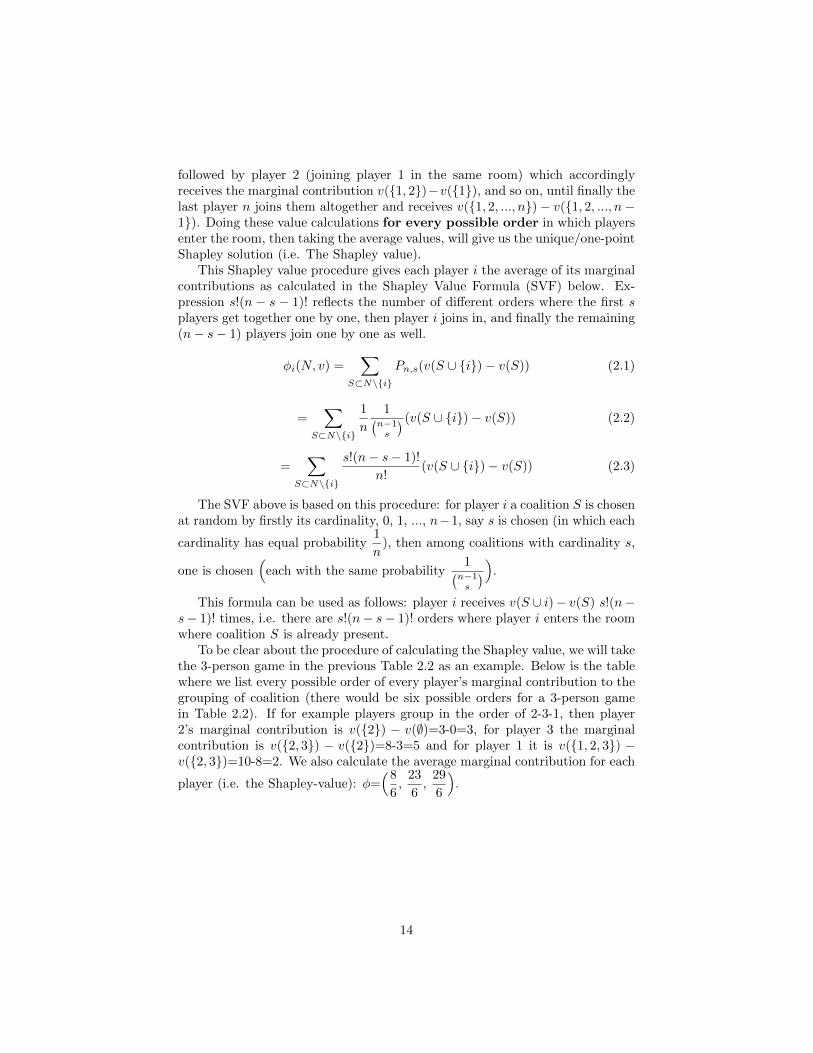
This Shapley value procedure gives each player i the average of its marginalcontributions as calculated in the Shapley Value Formula (SVF) below. Ex-pression s!(n − s − 1)! reflects the number of different orders where the first splayers get together one by one, then player i joins in, and finally the remaining(n− s− 1) players join one by one as well.

φi(N, v) =∑

S⊂N\i

Pn,s(v(S ∪ i)− v(S)) (2.1)

=∑

S⊂N\i

1

n

1(n−1s

) (v(S ∪ i)− v(S)) (2.2)

=∑

S⊂N\i

s!(n− s− 1)!

n!(v(S ∪ i)− v(S)) (2.3)

The SVF above is based on this procedure: for player i a coalition S is chosenat random by firstly its cardinality, 0, 1, ..., n−1, say s is chosen (in which each

cardinality has equal probability1

n), then among coalitions with cardinality s,

one is chosen(

each with the same probability1(n−1s

)).

This formula can be used as follows: player i receives v(S ∪ i)− v(S) s!(n−s− 1)! times, i.e. there are s!(n− s− 1)! orders where player i enters the roomwhere coalition S is already present.

To be clear about the procedure of calculating the Shapley value, we will takethe 3-person game in the previous Table 2.2 as an example. Below is the tablewhere we list every possible order of every player’s marginal contribution to thegrouping of coalition (there would be six possible orders for a 3-person gamein Table 2.2). If for example players group in the order of 2-3-1, then player2’s marginal contribution is v(2) − v(∅)=3-0=3, for player 3 the marginalcontribution is v(2, 3) − v(2)=8-3=5 and for player 1 it is v(1, 2, 3) −v(2, 3)=10-8=2. We also calculate the average marginal contribution for each

player (i.e. the Shapley-value): φ=(8

6,

23

6,

29

6

).

14

Table 2.8: Shapley value of the 3-person cooperative game

Possible orders 1 2 31-2-3 1 3 61-3-2 1 5 42-1-3 1 3 62-3-1 2 3 53-1-2 1 5 43-2-1 2 4 4

column sums 8 23 29φ 8

6236

296

Solution 2: Utopia Value

We now define the Utopia value of a cooperative n-person game, a one-pointsolution concept that is a part of a solution concept introduced by Stef Tijs(1981) [19] called the τ value. Let N be the set of all players and v(N) be thevalue of the grand coalition. Given nonempty coalition S ⊆ N and player i ∈ N ,let bi := v(N) − v(N \ i) be the utopia vector of player i, which expresses themarginal contribution of player i to the grand coalition.

This utopia vector b gives an intuitive upper limit to what a player mayexpect to obtain from participating in the game. Player i would like to receiveas much as his upper value, and he cannot hope for more than this value.Generally, every player will end up getting less than his utopia value, becausefor all interesting games, v(N) ≤ b1 + ...+ bn. If player i can get more than itsutopia vector bi, the other players might consider to throw i from the coalitionas they would be better off without i [21]. Therefore in a core allocation, noplayer can ever get a payoff that exceeds this upper value.

However, the utopia vector b may not be efficient: summing up all themarginal contributions

∑i∈S

bi of every player i ∈ N may not be equal to the

value of the grand coalition v(N). To satisfy the efficiency property, the valuethat is distributed to the players will be divided by the sum of all utopia vectorsfor all players in N . Thus we define the Utopia value in our procedure as follows:

UV (N, v) =( v(N)∑i∈N

bi

)b (2.4)

This utopia value is Shapley value-like, as its solution also has the additivityproperty. It also considers the marginal contributions, like the Shapley value.However, the utopia value takes only the marginal contribution regarding thegrand coalition into account, while the Shapley value also takes the marginalcontribution of all coalitions into account. Therefore this solution is simplerthan the Shapley value solution. [20]

15

Solution 3: Nucleolus

David Schmeidler (1969) in his paper ”The nucleolus of a characteristicfunction form game” [24] introduces the nucleolus as an alternative solutionfor cooperative games. The nucleolus is the set of individually rational alloca-tions that lexicographically minimizes the excess/dissatisfaction of all coalitions.Unlike the Shapley value, the nucleolus is a solution of a minimization problem[11]. It is unique but exists only when these individually rational allocationsexist; which in this case, if v(N) ≥

∑i∈N v(i). By definition, nucleolus will be

in the core of the game whenever the core is non-empty.Instead of applying a general axiomatization of fairness to a value function

defined on the set of all characteristic functions, we look at a fixed characteristicfunction v, and try to find an allocation x = (x1, ..., xn) that minimizes the worstinequity. That is, we ask each coalition S how dissatisfied it is with the proposedallocation x and we try to minimize the maximum dissatisfaction.

X is the nucleolus if and only if for all other allocations Z and all coalitionsT that are better off with Z (i.e.

∑i∈T

zi ≥∑i∈T

xi), there is a coalition T ′ that is

better off with X, and x-dissatisfaction of T ′ is at least as large as the one of T[25].

There is an intuitive procedure to find this nucleolus [9]. If the core isnon-empty, what we do is increasing the worth of all coalitions simultaneously,by the same amount, except for the empty set ∅ and the grand coalition N.This operation would make the new core become much smaller as we continueincreasing until a further increment would result in an empty new core. If inthe end a single point remains, then we got the nucleolus. Otherwise, if thereare two or more coalitions remain but we cannot increase any further withoutcreating an empty core (thus there are conflicting constraints), we then stopincreasing the worth of these conflicting coalitions and keep on increasing theworth of every other coalition. We proceed this way until finally, we have a coreconsisting of just one point, which is the nucleolus.

On the other hand, starting with an empty core, we simply decrease theworth of all coalitions simultaneously, again except for the emptyset and thegrand coalition, until we arrive at a game with a non-empty core. From thatmoment onwards, if we did not find a single point core, then we continue byincreasing the worth of the non-conflicting coalitions, until again some condi-tions are on the verge of conflicting each other. The increase of the worth ofconflicting coalitions is put on hold and we continue with the non-conflictingones till a single point core remains: the nucleolus.

The nucleolus is one of the allocations that minimizes the maximal excess, i.e.if for a game (N,v) an allocation x=(x1,...,xn) is being considered as a solution,then one might wish to measure the level of each coalition’s dissatisfaction withinthe possible solution. The difference between v(S ) and x (S ):=

∑i∈Sxi is taken

as a measure of the dissatisfaction for each coalition S, and is called the excesse(S,x ).

16

e(S, x) = v(S)− x(S) (2.5)

Note that each coalition would prefer a solution with the smallest excess aspossible.

The problem of minimizing the maximum of a collection of linear functionssubject to a linear constraint is easily converted to a linear programming prob-lem and can thus be solved by the simplex method, for example. After this isdone, one may have to solve a second linear programming problem to minimizethe next largest excess, and so on. However, it is beyond the scope of this thesis.

In our procedure that will be explained later in the next subsection, we applythe Prenucleolus solution, which is preferred by the math-oriented game theo-rists, instead of the nucleolus which is preferred by the game theorists. In mostcases, prenucleolus and nucleolus are considered the same. The difference withnucleolus is that there is no assumption of individually rational allocations whenprenucleolus is considered. In the nucleolus, we only consider the individuallyrational allocations by letting contribution for player i, xi ≥ v(i). While theprenucleolus only consider efficient allocations by looking at the contributionx ∈ RN for which

∑i∈N

xi = v(N).

Nucleolus and prenucleolus are overlapping in a class of nonnegative gameswhere this inequality v(T ) −

∑i∈T

v(i) ≤ v(S) −∑i∈S

v(i) holds [12] for the two

coalitions T ⊆ S. In our context, this inequality seems to hold. Therefore inthis thesis, we may say the nucleolus and prenucleolus are the same. To avoidconfusion, from now on we will call our solution concept as the Prenucleolus.

2.3 The Fitting Techniques

In the previous section, we already have three solution concepts in cooperativegame, namely the Shapley value, the Utopia value, and the Prenucleolus. To beable to reconstruct the game using the solution concepts given and the brooddata which will be explained in section 2.4, we need some techniques to beimplemented in our procedure of finding the best fitted game. Here we describehow can we make the game from the brood data that will be translated intosolutions, assuming this game is solved by the three solution concepts men-tioned earlier. To determine how good this game fits the solutions, we will alsointroduce an error measurement in this section.

2.3.1 Techniques on Shapley Value

As we mentioned before, Jean Derks [18] described three procedures in orderto find a fit for the brood data, making use of some mathematical conceptssuch as Balanced Contributions and Unanimity games. Below we will explainand examine how these approaches look like, then choose one of them to beimplemented in our brood data.

17

Firstly, let N be a fixed, finite set of players, and let Ω be a set of subsetsof N . Suppose for each coalition S ∈ Ω there is a payoff vector xS = (xSi )i∈S ,expressing the profits of the players in S when they decide to cooperate. Inother words, this xS is a set of solutions of a cooperative game. We address theproblem of how to find this corresponding cooperative game. Assuming thatthe payoffs follow the Shapley value distribution, the following approaches areconsidered.

Balanced Contributions

One approach is to assume some kind of fairness or balancedness that also holdsfor the Shapley value [26]. Consider a so-called payoff system Z = (zSi )S⊂N,i∈S .Z is said to be balanced if equation 3.2 below holds for all coalitions S andplayers i, j ∈ S.

zSi − zS\ji = zSj − z

S\ij (2.6)

The intuition behind this property is as follows: the amount zSi − zS\ji is

the loss player i experiences when player j decides to leave the coalition S; so,Z is balanced if each two players in any coalition attain the same loss when theother decide to leave the coalition.

Naturally, we may not be able to extend the above introduced collectionX = (xS)S∈Ω into a balanced payoff system Z but it is interesting to investigateconditions on Ω ensuring the existence of balanced extentions. This is, however,not pursued in this thesis.

Game-Fitting Procedure

For this procedural approach, we define a unanimity game for coalition S

US(T ) =

1 if S ⊆ T , T ⊆ N0 otherwise

(2.7)

These unanimity games U form a basis for the set of games that we will usein our procedure that will be explained in the next approach. In this unanimitygame, all players in S should be present in order to make the coalition T to bepowerful. The Shapley value for this unanimity game is given by:

φ(US) =

1

|S|if i ∈ S

0 otherwise(2.8)

Note that here we divide 1 with the number of players in S. We can see thatthe payoff vector φ(US) is now efficient.

Suppose that we fit the data and arrive at a game (N, v). How can weimprove the upcoming procedural approach in some sense ’better’. From theexisting game (N, v), we only consider new games (N, v + αu) with a scalar α,and u ∈ U , a finite, fixed set of games. As already mentioned before, here wetake U to be the set of unanimity games. For each unanimity game (N, uT ) we

18

first compute the weight αT for which the error is minimum, i.e. satisfying thisequation:

E(v + αTuT ) = minαE(v + αuT ). (2.9)

Then, choose coalition T with:

E(v + αTuT ) = minTE(v + αTuT ), (2.10)

and let v′ be v + αTuT .In other words, we only change the existing game (N, v) into a new game

(N, v′) in the direction of one unanimity game.We will explain more on this error E in the following subsection.

Error Measurement

After we compute the new game (N, v′) using the procedure above, we want tosee if this game is close to the game we are looking for. Firstly, we will define twomeasures of ’closeness’. The first measurement eD is where we compare eachbrood data points with each solution points of the Shapley value procedurein order to measure how well the game solutions fit the brood data we have.The second one is E(v), in which we measure how well the brood data fits thesolutions of the new game we found from the fitting procedure. Assume thatthe importance weights IS∈Ω, are provided from the brood data; the smallerthe error E(v), the closer we would like the value of the coalitions v(S) to ourpayoff vectors xS . The following error measure fulfills this property:

E(v) =

∑S∈Ω

IS

∣∣∣∑i∈S

xSi − v(S)∣∣∣∑

i∈SxSi∑

S∈Ω

IS(2.11)

Note that we firstly take the absolute error in order to avoid negative results inthe summation, then we take the mean by dividing this absolute error with thetotal of our payoff vectors. We then take the relative error by multiplying theabsolute error with the importance weights of every possible coalitions S in Ω.Finally we divide it with the sum of the importance weights, to get the totalerror measurement.

For the error measure eD, we calculate the difference between the new game(ySi∈S)

S∈Ωwith our payoff vector. This ySi is defined as the Shapley value

solution of the subgame v with weight w (see next subsection for this weightedversion), in which only players in S are taken into account. The error eD ismathematically define as follows:

eD =

∑S∈Ω

IS

√∑i∈S

(xSi − ySi )2

∑S∈Ω

IS(2.12)

19

We firstly take the square of the difference in order to avoid negative values,sum it over all players in S, then take the square root before multiplying it withthe sum of the importance. In the end, we also divide the result with the sumof all importance weights.

Here we take ySi =99

100xSi to be the new game in order to get the 1% average

of error as a value that we would like to achieve.The error E(v) is smallest among all games derived from v by adding a

weighted unanimity game. By repeating the game-fitting procedure above, forexample by starting with the zero game, we may arrive at a game with errorbelow a given level, or when the error change is below a specified level (forexample 0.0001 of the desired error level). This error E(v) is our focus on theexperiments later, as the smallest E(v) would bring us closer to the best fittedgame in which the value of the coalitions v(S) is close to our payoff vectors xS .

Weighted Shapley Value

If the resulting error is still high, and in order to capture the problem thatdifferent players evaluate the payoff differently, instead of using the unanimitygame in the above repeated procedure where the payoffs to the players aretreated equally, we may consider the weighted Shapley value approach [27]. Byassuming that there are (unknown) weights wi, i ∈ N , such that the payoff ofone unit is actually worth wi to player i, then we should consider the set ofallocations:

xw =( 1

w ixSi

)i∈S,S∈Ω

(2.13)

in the above approach.Let E(v) denotes the error and vw the game we get if we apply the repeated

procedure on xw. It can be proven that E(v) equals the error on vw, but insteadof the Shapley value the weighted Shapley value is chosen with weight systemwi.

In computing weights with a satisfactory error we may follow the same ideaas before. Let W = w1, ..., wK be a set of weight systems:for each weight system wk compute the weight αK , α:=0 to 1, for which

E(w + αkwk) = minαE(w + αwk). (2.14)

Then, choose index k with

E(w + αkwk) = minTE(w + αkw

k). (2.15)

and let w′ be w + αkwk.

Again, by repeating this procedure, for example by starting with weightswi = 1, i ∈ N , we may arrive at a game with desirable error.

Naturally, the weight systems in W may be chosen such that the neededcomputations are effectively implemented. However, no such W is known, andtherefore we propose the following procedure, with α a given positive number.

20

As long as there is a wk ∈ W such that E(v) > E(w + αwk) then change vinto w + αwk. If no improvements are observed then change α into a smallernumber, then repeat this procedure. The repetition can be maintained as longas computation time is available or the desirable error is reached.

2.3.2 Other Solution Concepts as Comparison

In order to compare the performance of the Shapley value procedure in ourbrood data, a similar fitting procedure is applied on the weighted version of theother two approaches (i.e. the Utopia value and the Prenucleolus). Note thatwe will not explain the techniques for these two other solution concepts as thesame approaches described for the Shapley value above are mimicked for bothUtopia value and Prenucleolus.

2.4 The Data and The Game Translation

In this section we will describe what are the data we have and how can wetranslate the raw data using the model and the techniques explained in theprevious sections, into something useful and insightful.

2.4.1 The Brood Data

The brood datasets that are used in this thesis have been collected by ProfessorScott Forbes for about ten years during his research in wetlands near Winnipeg,Manitoba, Canada. It is defined in Forbes book [1] that the core brood/chicksare the nestlings that are hatched together on the first day of the nestlingperiod; while nestlings that are hatched one or more days later are defined asthe marginal brood/chicks. The blackbird parents’ choice of hatching how manyeggs in the first day could be based on their experiences on the previous hatchingperiods, or on their instinct of the weather and food condition near the nest.They will hatch each one of the marginal every one day after the core. Thus,having 2 core chicks and 3 marginals will make the hatching periods of 4 daysin total (1 day for all the cores, 3 additional days for each marginal).

The raw data in Table 2.9 and Table 2.10 below enable us to find out howmany core and marginal children that the blackbirds could have in one brood,as well as how many broods are available for the specific number of core andmarginal chicks. We can also see how many chicks that are perished duringone week of measurement (starting from day 1 to day 8). These large datasetshave been compiled into good years and bad years period, which allow us to seewhether there is any difference on how parents allocate the food for the coreand marginal children during the good and the bad times.

Note that notation #eggs shows how many eggs are firstly available intotal before the hatching period. These eggs might be removed, broken, orperish early during a hatching failure, thus this total number can sometimesbe different with the number of hatchlings. Notation c in day 1, denotes the

21

number of core eggs (eggs that are hatched in day 1) inside one brood; whilenotation m denotes the number of marginal eggs (eggs that are left/not yethatched in day 1) in one brood. Notation #br shows how many broods thatare available in total. In day 8, c and m denote number of core and marginalchicks which survive within one week, while m1, m2, m3 denote the number ofmarginals that are hatched on the first, the second, and on the third day afterthe core. The total in day 8 shows how many chicks that are continue livingafter one week of feeding.

Table 2.9: The good years raw data

day 1 day 8#eggs c m #br c m m1 m2 m3 total

18 1 0 15 15 0 0 0 0 1559 1 1 29 27 27 27 0 0 53120 1 2 40 38 62 33 29 0 95218 1 3 55 54 124 52 48 24 17630 2 0 15 28 0 0 0 0 28236 2 1 78 134 56 56 0 0 186430 2 2 108 208 140 85 55 0 34575 2 3 15 29 26 14 9 3 5581 3 0 27 74 0 0 0 0 74292 3 1 73 196 33 33 0 0 224100 3 2 20 55 16 12 3 0 7132 4 0 8 27 0 0 0 0 2725 4 1 5 19 2 2 0 0 21

Table 2.10: The bad years raw data

day 1 day 8#eggs c m #br c m m1 m2 m3 total

6 1 0 6 6 0 0 0 0 640 1 1 20 22 17 16 1 0 35100 1 2 33 39 48 26 22 0 63116 1 3 29 46 56 27 22 6 6850 2 0 24 46 0 0 0 0 46153 2 1 51 104 35 34 0 0 121292 2 2 73 136 61 44 17 0 16855 2 3 11 19 13 9 3 1 2954 3 0 18 44 0 1 0 0 44331 3 1 83 201 25 25 0 0 19840 3 2 8 23 1 1 0 0 2228 4 0 7 21 0 0 0 0 2115 4 1 3 9 1 1 0 0 10

As we have seen in the above data, one brood can contain at maximum 4 corechicks, while on the other hand, it can also contain at maximum 3 marginals.

22

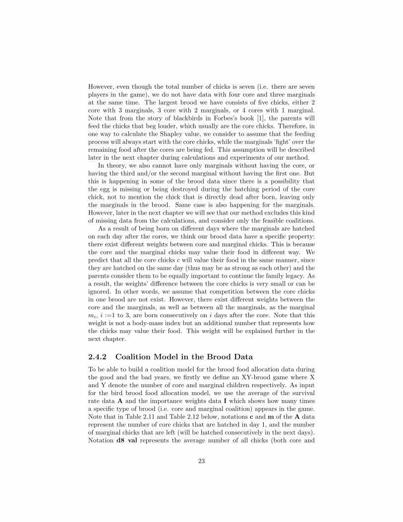
However, even though the total number of chicks is seven (i.e. there are sevenplayers in the game), we do not have data with four core and three marginalsat the same time. The largest brood we have consists of five chicks, either 2core with 3 marginals, 3 core with 2 marginals, or 4 cores with 1 marginal.Note that from the story of blackbirds in Forbes’s book [1], the parents willfeed the chicks that beg louder, which usually are the core chicks. Therefore, inone way to calculate the Shapley value, we consider to assume that the feedingprocess will always start with the core chicks, while the marginals ’fight’ over theremaining food after the cores are being fed. This assumption will be describedlater in the next chapter during calculations and experiments of our method.

In theory, we also cannot have only marginals without having the core, orhaving the third and/or the second marginal without having the first one. Butthis is happening in some of the brood data since there is a possibility thatthe egg is missing or being destroyed during the hatching period of the corechick, not to mention the chick that is directly dead after born, leaving onlythe marginals in the brood. Same case is also happening for the marginals.However, later in the next chapter we will see that our method excludes this kindof missing data from the calculations, and consider only the feasible coalitions.

As a result of being born on different days where the marginals are hatchedon each day after the cores, we think our brood data have a specific property:there exist different weights between core and marginal chicks. This is becausethe core and the marginal chicks may value their food in different way. Wepredict that all the core chicks c will value their food in the same manner, sincethey are hatched on the same day (thus may be as strong as each other) and theparents consider them to be equally important to continue the family legacy. Asa result, the weights’ difference between the core chicks is very small or can beignored. In other words, we assume that competition between the core chicksin one brood are not exist. However, there exist different weights between thecore and the marginals, as well as between all the marginals, as the marginalmi, i :=1 to 3, are born consecutively on i days after the core. Note that thisweight is not a body-mass index but an additional number that represents howthe chicks may value their food. This weight will be explained further in thenext chapter.

2.4.2 Coalition Model in the Brood Data

To be able to build a coalition model for the brood food allocation data duringthe good and the bad years, we firstly we define an XY-brood game where Xand Y denote the number of core and marginal children respectively. As inputfor the bird brood food allocation model, we use the average of the survivalrate data A and the importance weights data I which shows how many timesa specific type of brood (i.e. core and marginal coalition) appears in the game.Note that in Table 2.11 and Table 2.12 below, notations c and m of the A datarepresent the number of core chicks that are hatched in day 1, and the numberof marginal chicks that are left (will be hatched consecutively in the next days).Notation d8 val represents the average number of all chicks (both core and

23

marginals) which survive until one week of feeding (i.e. day 8). Notation m avshows the average of the marginal chicks’ survival rate which we will use to fillthe coalition value for the marginals later in our method, while each notations cval, m1 val, m2 val, and m3 val show the survival rate of each chick, startingfrom the core, the first marginal, until the third marginal chick respectively.

Table 2.11: Average of the Survival Rate for XY-brood type during the Goodyears

Ac m c val m av m1 val m2 val m3 val d8 val I1 0 1.000 1.000 161 1 0.931 0.931 0.931 1.862 291 2 0.950 0.838 0.892 0.784 2.626 401 3 0.982 0.765 0.963 0.889 0.453 3.287 552 0 0.933 1.867 152 1 0.859 0.747 0.747 2.465 782 2 0.963 0.688 0.794 0.514 3.234 1082 3 0.967 0.578 0.933 0.600 0.200 3.667 153 0 0.914 2.741 273 1 0.895 0.465 0.465 3.150 733 2 0.917 0.400 0.632 0.158 3.539 204 0 0.844 3.375 84 1 0.950 0.400 0.400 4.200 5

Table 2.12: Average of the Survival Rate for XY-brood type during the Badyears

Ac m c val m av m1 val m2 val m3 val d8 val I1 0 1.000 1.000 61 1 1.000 0.850 0.850 1.850 201 2 0.848 0.774 0.839 0.710 2.397 331 3 1.000 0.644 0.931 0.759 0.453 2.897 292 0 0.958 1.917 242 1 0.931 0.686 0.686 2.549 512 2 0.836 0.418 0.603 0.233 2.507 732 3 0.818 0.433 0.900 0.300 0.200 2.936 113 0 0.815 2.444 183 1 0.763 0.309 0.309 2.598 833 2 0.917 0.063 0.125 0.000 2.875 84 0 0.750 3.000 74 1 0.750 0.333 0.333 3.333 3

Having the coalitions S, what value can we choose to be the value of thecoalition v(S)? Since we have the average of the survival rate A for each off-springs in every XY-brood, taking into account its importance weight I (i.e. how

24

many times the XY-brood data occur), we can take these values as the value ofthe coalitions. But how to put the ’right’ value into the ’right’ coalition? Herewe propose a coalition procedure which we adapt from the Shapley value proce-dure in the previous subsection by seeing the problem as a coalitional procedureas shown in the example given in subsection 2.1.3.

1. Suppose we have an XY-brood game during either the good or the badyears, with maximum 7 players (i=1 to 7), consists of maximum 4 core(i=1 to 4) and maximum 3 marginal players (i:=5 to 7). Firstly we defineall possible coalitions of (X+Y) players where there are X core players andY marginals.

For example, if we take the good years 21-brood data where there are twocore players and one marginal player, it is possible to have coalitions ofevery single player, coalition between the core players, coalitions betweeneach core with the marginal, and coalition of all the three players. In otherwords, for the good years 21-brood, the possible coalitions of the 3 playersare: 1, 2, 5, 1,2, 1,5, 2,5, and 1,2,5.

2. We then re-translate every possible coalition into the number of core andmarginal players in a brood.

For example, coalition 1 and 2 is when we only have one core playerin a brood, without having any marginals; i.e. the 10-brood. Thus, for thesingle core player coalitions, we will consider the 10-brood game. Now wedo the same translations for the other coalitions: consider 20-brood gamefor the coalition between the core players 1,2, 11-brood game for thecoalitions of each core player with the marginal (i.e. 1,5 and 2,5), andsimply 21-brood game itself for the coalition of all three players 1,2,5.As an exception, for the marginal player coalition 5 in 21-brood data,we cannot take the 01-brood into account, since by definition, no marginalcan be hatched before having the core hatched. Thus we do not need toconsider this kind of brood in the procedure.

3. Now we continue by looking at Table 2.11 for the good years, and Table2.12 for the bad years, in order to see the average of the survival ratein the corresponding XY-brood data, which we need to consider for eachcoalition.

As an example, to fill in the coalition value v(S) of the single core playercoalitions 1 and 2, we take the average of the survival rate for thiscore chick in 10-brood, which is 1.000 (see c val on the table). For themarginal player coalition 5 which is an exception, we choose to take thesurvival rate of the marginal on its first appearence in the brood datasets,which is the m1 val value on table: 0.931. Note that this m1 val is equalto the m val as we only have one marginal in 10-brood game. For the20-brood, 11-brood, and 21-brood game, we take the corresponding totalaverage number of the chicks’ survival rate d8 val, which are 1.867, 1.862,and 2.465, respectively.

25

As a result, we then have this coalition table for the 21-brood game duringthe good years period:

Table 2.13: 21-brood game, good years

S 1 2 5 1,2 1,5 2,5 1,2,5v(S) 1.000 1.000 0.931 1.867 1.862 1.862 2.465

Note that we remove the emptyset coalition (∅) in the brood coalition tablesince in any case it would always take a zero value. Same procedure applies forevery XY-brood game.

26

Chapter 3

Experiments

Before adapting the brood data into a program, we think it is better to getthe feeling of how the brood data looks like; so that we know what is the bestchoice to implement this data into the program. Therefore in this chapter,firstly we will show how we do some calculations by hand on the Shapley valuesolutions for some XY-brood game in the good and the bad years data. Afterthat, we will provide some results of the experiments using Matlab for thethree solutions described in the previous chapter, namely the Shapley value, theUtopia value, and the Prenucleolus, using two different cooperation approachescalled the standard approach and the restricted approach. We will also showhow we translate the survival rate into some kind of utility functions and whichtranslation gives the best fit with the smallest minimum error. We are usingthe good and the bad years data that have been compiled by Professor ScottForbes, as well as random data for validation. Our focus is onto the Shapleyvalue, but we will compare its results with the other two solution concepts.

3.1 Calculations by Hand

Here in this section, we will show that for some cases of the brood data in thegood and the bad years period, it is possible to calculate the Shapley valuesolution by hand. However, the larger the data, the more we need a programwhich can easily find the solutions using the Shapley value solution concept, orthe other cooperative game solution concepts in a quite short period of time.

3.1.1 Calculating Shapley Value of the Good Years Data

As we can see in the brood data for the good years (Table 2.11), there are dataof 10-brood, 11-brood, 12-brood, 13-brood, 20-brood, 21-brood, 22-brood, 23-brood, 30-brood, 31-brood, 32-brood, 40-brood, and 41-brood. To get a feelingof these data we are having, we will calculate the Shapley value φ by hand forsome of the smaller broods data, to see if we can get something interesting as a

27

result.There are two different approaches that we use in our procedure of calcu-

lating the payoff vectors xS for the coalition S. The first one is the standardapproach. Remember that we have at maximum seven players (|N |=7), consistof at maximum 4 core players (i=1 to 4) and at maximum 3 marginal players(i:=5 to 7). Thus, we may consider seven different places for each different po-sitions of the players. In this standard approach, the core chicks can be placedin anywhere among the four first places while the marginals are placed consecu-tively in the three last places (in an increasing order). As the core may becomethe first, the second, the third, or the fourth player, it can be placed in anyof the four first places. Thus, we need to consider the same survival rates forall these four possible places of the core chicks in each XY-brood game; whilethe importance weights I for the corresponding core chicks are divided equallyamong the four possible places. Note that whichever chick chooses the firstplace will be considered as the first core, and so on.

To be clear about this representation, we convert Table 2.11 of the good yearsdata into a new table, Table 3.1, by defining an allocation xS as the averageof every chick’s survival rate in the corresponding XY-brood game, taking intoaccount the possible coalitions that can be made by all the players involved inthe game. For example, if we consider the good years 21-brood game using thestandard approach, we will have a set of possible coalitions which consists ofcoalition 1,2,5, 1,3,5, 1,4,5, 2,3,5, 2,4,5, and 3,4,5 since the twocore chicks can choose any of the four first places. Note that what we denote aspossible coalitions here are the places where the chicks exist.

The Table 3.1 below will show how many players involved in each coalitionof a specific XY-brood, what are the possible coalitions exist in a specific XY-brood, and what are the survival rates of each player involves in those specificcoalitions. Note that the numbers i:=1 to 7 in the table denote the players,where i=1 to 4 are core players and i:=5 to 7 are marginal players.

28

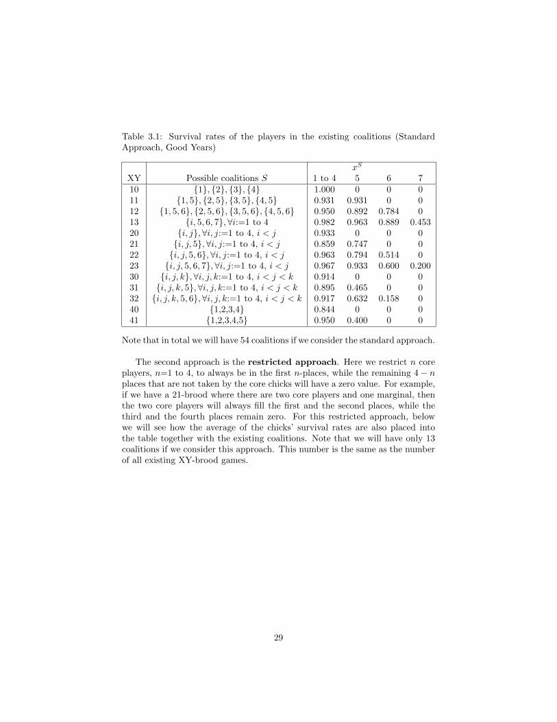
Table 3.1: Survival rates of the players in the existing coalitions (StandardApproach, Good Years)

xS

XY Possible coalitions S 1 to 4 5 6 710 1, 2, 3, 4 1.000 0 0 011 1, 5, 2, 5, 3, 5, 4, 5 0.931 0.931 0 012 1, 5, 6, 2, 5, 6, 3, 5, 6, 4, 5, 6 0.950 0.892 0.784 013 i, 5, 6, 7,∀i:=1 to 4 0.982 0.963 0.889 0.45320 i, j,∀i, j:=1 to 4, i < j 0.933 0 0 021 i, j, 5,∀i, j:=1 to 4, i < j 0.859 0.747 0 022 i, j, 5, 6,∀i, j:=1 to 4, i < j 0.963 0.794 0.514 023 i, j, 5, 6, 7,∀i, j:=1 to 4, i < j 0.967 0.933 0.600 0.20030 i, j, k,∀i, j, k:=1 to 4, i < j < k 0.914 0 0 031 i, j, k, 5,∀i, j, k:=1 to 4, i < j < k 0.895 0.465 0 032 i, j, k, 5, 6,∀i, j, k:=1 to 4, i < j < k 0.917 0.632 0.158 040 1,2,3,4 0.844 0 0 041 1,2,3,4,5 0.950 0.400 0 0

Note that in total we will have 54 coalitions if we consider the standard approach.

The second approach is the restricted approach. Here we restrict n coreplayers, n=1 to 4, to always be in the first n-places, while the remaining 4− nplaces that are not taken by the core chicks will have a zero value. For example,if we have a 21-brood where there are two core players and one marginal, thenthe two core players will always fill the first and the second places, while thethird and the fourth places remain zero. For this restricted approach, belowwe will see how the average of the chicks’ survival rates are also placed intothe table together with the existing coalitions. Note that we will have only 13coalitions if we consider this approach. This number is the same as the numberof all existing XY-brood games.

29

Table 3.2: Survival rates of the players in the existing coalitions (RestrictedApproach, Good Years)

xS

XY-brood S 1 2 3 4 5 6 710 1 1.000 0 0 0 0 0 011 1,5 0.931 0 0 0 0.931 0 012 1,5,6 0.950 0 0 0 0.892 0.784 013 1,5,6,7 0.982 0 0 0 0.963 0.889 0.45320 1,2 0.933 0.933 0 0 0 0 021 1,2,5 0.859 0.859 0 0 0.747 0 022 1,2,5,6 0.963 0.963 0 0 0.794 0.514 023 1,2,5,6,7 0.967 0.967 0 0 0.933 0.600 0.20030 1,2,3 0.914 0.914 0.914 0 0 0 031 1,2,3,5 0.895 0.895 0.895 0 0.465 0 032 1,2,3,5,6 0.917 0.917 0.917 0 0.632 0.158 040 1,2,3,4 0.844 0.844 0.844 0.844 0 0 041 1,2,3,4,5 0.950 0.950 0.950 0.950 0.400 0 0

After having the two tables above, we will explain two ways of calculatingthe Shapley value φ for 12-brood by hands. The first one is done for everypossible orderings of the grand coalition, while the second one is by removingthe orders that are assumed to be unfeasible before we start calculating thevalue. To understand how this calculation method works, we will denote a setof possible orders P as any possible orders of the chicks when they are beingfed by the parents: starting from the firstly fed chick, until every chick in thecorresponding XY-brood data is being fed. For example, order 1-5-6 in the 12-brood game means that the core chick is being fed at the first place, followedby the first and the second marginals consecutively.

As we have mentioned in the previous chapter,when blackbirds parents cometo the nest bringing the foods for their chicks, whichever chick that begs harderwill be fed first with usually the largest amount of food, and vice versa; chickthat is being fed last will get just the remainder. As food given from parentsis probably the only source of the chicks’ nutritions, at least until they areable to fly and look for another source of food, this food is very important forthem to survive. Therefore, we may logically assume that the chick’s order ofbeing fed will affect their survival rate. Using this assumption, it is possible tocalculate the Shapley value by taking the average of the chicks’ survival rate inthe corresponding brood data to be interpreted as the amount of food the chicksare getting from their parents which will help them to survive. An average of1.000 for a chick’s survival rate could be translated as: the chick is getting 100%of food that it needs to survive.

In order to calculate the Shapley value by hand using the translation above,we define the following allocation procedure:

30

1. Consider the XY-brood game during either the good or the bad yearsperiod under the restricted approach. Make a coalition table for the XY-brood game using the coalition procedure described in subsection 2.4.2.

As an example, now we consider the good years 12-brood game. Usingthe procedure that are explained before in section 2.4.2 and looking atTable 2.11 for the chicks’ average survival rate data during the good years,notice that we use the total sum of all chicks’ survival rate in 12-brood tofill in the value of the grand coalition, while the marginals’ average m avof the 11-brood and 12-brood are used to fill in the value of the coalition5 and 6, respectively. To fill in the value for coalition 1,5 and 1,6,we use the sum of the survival rate for core chick in 11-brood with the mav of 11-brood and 12-brood respectively. Finally, the sum of m1 and m2

survival rate of the 12-brood is used to fill in the value for coalition 5,6.Thus, we have a coalition table for the 12-brood game as follows:

Table 3.3: 12-brood game, good years

S 1 5 6 1,5 1,6 5,6 1,5,6v(S) 1.000 0.931 0.838 1.862 1.769 1.676 2.626

2. List every possible orders of the grand coalition that correspond to thisXY-brood data.

3. In order to be able to fill in the ’right’ value that every player will getaccording to their possible ordering, we adapt the same Shapley procedureas explained in the previous chapter. This way, we will divide the valueof the grand coalition ’fairly’ by considering the orders and the value thatare ’claimed’ by each coalition.

As an example, from Table 3.3, we know that player 1 in coalition 1is ’claiming’ an average of 1 for its survival rate, while player 5 and 6in coalition 5 and 6 are ’claiming’ an average of 0.931 and 0.838,respectively. If we take into account order 1-5-6 of the players in thegrand coalition, we will firstly allocate 1.000 for player 1; exactly thesame amount as what it claims. To decide how much should player 5 gets,we look at Table 3.3 and see that 1.862 is the value of coalition 1,5.Since we already give player 1 a value of 1.000, the remaining value of0.862 will be the amount which is given to player 5. Keep in mind thatthe sum of every player’s value needs to be equal to the value of the grandcoalition. Since a total of 1.862 has already been given to player 1 and 5,player 6 will get the remainder of the grand coalition value; which is 0.764.Doing the same procedures to every possible orders, we will get a Shapleyvalue calculation table as shown below. Note that notation φ denotes theShapley value of each player involved in the grand coalition.

31

Table 3.4: Shapley value of 12-brood game, good years

Possible orders Player TotalP 1 5 6

1-5-6 1.000 0.862 0.7641-6-5 1.000 0.857 0.7695-1-6 0.931 0.931 0.7645-6-1 0.950 0.931 0.7456-1-5 0.931 0.857 0.8386-5-1 0.950 0.838 0.838φ 0.960 0.879 0.786 2.626

4. Now we compare the values we got from observing the average survivalrates of each chick in the corresponding XY-brood data, which we denoteas Observ., to the Shapley values we got from calculation. In order to getthese observation values, we need to look at Table 3.2 (restricted approach)and find the average survival rate of each chick in the corresponding XY-brood.

For example, the observation values for player 1, player 5, and player6 in 12-brood game according to Table 3.2 are 0.950, 0.892, and 0.784,respectively. For easier comparison, we will add these observation valuesinto the Shapley value calculation table we made in the previous step,resulting this table below:

Table 3.5: Possible orders for 12-brood game, good years

Possible orders Player TotalP 1 5 6

1-5-6 1.000 0.862 0.7641-6-5 1.000 0.857 0.7695-1-6 0.931 0.931 0.7645-6-1 0.950 0.931 0.7456-1-5 0.931 0.857 0.8386-5-1 0.950 0.838 0.838φ 0.960 0.879 0.786 2.626

Observ. 0.950 0.892 0.784 2.626

5. Since there is almost no case in the blackbird broods where the marginalchicks are being fed before the core chicks, now we consider to leave outthe unfeasible orders from the Shapley value calculation table and consideronly the cases when the core chicks are being fed before the marginals. Wenow have a new Shapley value calculation table with a set of feasible ordersF instead of possible ones. Below is the new Shapley value calculationtable for the 12-brood game:

32

Table 3.6: Feasible orders for 12-brood game, good years

Feasible orders Player TotalF 1 5 6

1-5-6 1.000 0.862 0.7641-6-5 1.000 0.857 0.769φ 1.000 0.8595 0.7665 2.626

Observ. 0.950 0.892 0.784 2.626

Again, we compare the Shapley value φ with the observation value to seeif parental favoritism exists in the case of a specific XY-brood data.

Notice that in the case of 12-brood, the Shapley values φ for the core chicksthat we got in both cases are larger than the observation values. Thus there isno tendency of parents favoriting the core chicks according to this Shapley valuesolution in 12-brood. On the other hand, the Shapley value for the marginalsare almost always larger in the observations rather than in the calculation;except for the second marginal in the case of taking all possible orders P intocalculation. Thus we may say that in the good years 12-brood data, there isno indication of blackbirds parents playing favorites between the core and themarginal chicks.

Would it still be the case for every XY-brood game during the good years,or will the parents start favoriting the core chicks at some point? Note that thesame way of calculations can also be applied for every brood game, especiallythe smaller ones (with not more than three or four players in one brood).

Here we provide another example in the good years data using the aboveShapley value calculation procedure to see if parental favoritism could exist evenin the good years. Consider the 21-brood game under the restricted approachwhere there exists two core chicks as player 1 and 2, and one marginal as player5. Following the same Shapley value calculation procedure, ordering the chicksin 21-brood into order 1-5-2 means that we firstly give allocation for coalition1,3 (by giving allocation for chick 1 first from v(1, 5) and the rest for chick5), then lastly give the rest of the grand coalition value v(1, 5, 2) for chick 2after being reduced by v(1, 5).

Table 3.7 below will list all possible orders as well as the Shapley value forthe 21-brood game mentioned earlier in the previous chapter (see Table 2.13for all the possible coalition values of this 21-brood game). In the end, we alsocompare the value we got with our observation value for the 21-brood data (seethe corresponding average of the survival rate for each chick involves in the21-brood game from the A data). Note that the sum of the observed averageof all chicks’ survival rate in the corresponding game (see d8 val data in table2.11) is equal to the value of the grand coalition.

33

Table 3.7: Possible orders for 21-brood game, good years

Possible orders Player TotalP 1 2 5

1-2-5 1,000 0,867 0,5981-5-2 1,000 0,603 0,8622-1-5 0,867 1,000 0,5982-5-1 0,603 1,000 0,8625-1-2 0,931 0,603 0,9315-2-1 0,603 0,931 0,931φ 0,834 0,834 0,797 2,465

Observ. 0,859 0,859 0,747 2,465

From Table 3.7, we see that the marginal chick gets a little bit less than itsShapley value solution, while the cores get a little bit more in the observation. Itmeans that according to the Shapley value solution concept and by consideringevery possible orders of feeding the chicks in the good years 21-brood, we maysay that the parents are quite ’favoriting’ the core ones.

Now we will leave out the unfeasible orders and consider only the feasibleones. According to our assumption in subsection 2.4.1 that the parents willfeed the core chicks firstly before the marginals, we can interchange only theorder of the core chicks or the order of the marginals. Coalitions in which anymarginal is fed before any core are not feasible. Thus, erasing orders 1-5-2,2-1-5, 5-1-2, and 5-2-1 from our calculations will give us the table below:

Table 3.8: Feasible orders for 21-brood game, good years

Feasible orders TotalF 1 2 5

1-2-5 1,000 0,867 0,5982-1-5 0,867 1,000 0,598φ 0,9335 0,9335 0,598 2,465

Observ. 0,859 0,859 0,747 2,465

We can see in Table 3.8 that if we remove the unfeasible coalition ordersusing our assumption in subsection 2.2.1, the result is the other way around.Here the marginal gets much more in reality rather than what it suppose to getbased on the Shapley value solution that we calculate.

Now we are questioning about the bad years: would the parental favoritismalso appears in the bad years? And if so, would it happen even worse ratherthan in the good years? We will provide an answer to these questions in thenext section.

Interestingly, we can also check whether our Shapley value solutions for thetwo good years brood games above satisfy the property of a CG-solution asdescribed in subsection 2.1.3: the one who claims more, will never get less orlose less than the one who claims less. Therefore, we need to check these twoconditions on our Shapley value solutions:

34

1. Whether the one claiming more will always gets more than the one claim-ing less

2. And whether the one claiming more will always loses more than the oneclaiming less,

For the case of good years 12-brood game, from Table 3.3 we can see that solely,player 1, 5, and 6 are claiming 1.000, 0.931, and 0.838, respectively. This means,player 1 claims the most, while player 6 claims the least. When consideringall possible orders P, the Shapley value solutions are 0.960, 0.879, and 0.786,respectively. Since according to these solutions player 1 gets the most whileplayer 6 gets the least, the first property of the CG-solution is satisfied.

However, when we consider the lose (i.e. the difference between the claimand the reward) that every players have, player 1 loses 0.040, while player 5 and6 equally lose 0.052. The lose of player 1 who claims the most, is in fact smallerthan the lose of two other players who claim less. Thus, the second property isunfortunately not satisfied. Therefore, when considering all the possible ordersinto the calculation, this Shapley value solutions of the good years 12-broodgame is not a CG-solution. We can also easily check for the case of removingthe unfeasible orders, and may arrive at the same conclusion.

In the case of the good years 21-brood game, we also get the same conclusionswhen considering only the feasible orders into the Shapley value calculation.However, we get a different result when we consider all the possible orders.Claiming 1.000, 1.000, and 0.931 respectively according to Table 2.13, player1 and player 2 equally get 0.834, while player 5 gets 0.797 in their Shapleyvalue solutions. Claiming the most, player 1 and 2 lose 0.166, while player 5loses 0.134. We can easily see that this time, the two properties are satisfied.Thus, we may say that the Shapley value solutions of the good years 21-broodgame is a CG-solution when we consider all the possible feeding orders into thecalculation.

3.1.2 Calculating Shapley Value of the Bad Years Data

Before we give an example of Shapley value calculation that shows whetherthe parental favoritism exists even worse in the blackbird family during the badyears, we will provide two tables showing the chicks’ average survival rates usingthe two approaches: the standard and the restricted approach. Note that thesetwo tables are adapted from Table 2.12 in the same way as we adapt the tablefor the good years in the previous section.

35

Table 3.9: Survival rates of the players in the existing coalitions (StandardApproach, Bad Years)

xS

XY S 1 to 4 5 6 710 1, 2, 3, 4 1.000 0 0 011 1, 5, 2, 5, 3, 5, 4, 5 1.000 0.850 0 012 1, 5, 6, 2, 5, 6, 3, 5, 6, 4, 5, 6 0.848 0.839 0.710 013 1, 5, 6, 7, 2, 5, 6, 7, 3, 5, 6, 7, 4, 5, 6, 7 1.000 0.931 0.759 0.2020 i, j,∀i, j:=1 to 4, i < j 0.958 0 0 021 i, j, 5,∀i, j:=1 to 4, i < j 0.931 0.686 0 022 i, j, 5, 6,∀i, j:=1 to 4, i < j 0.836 0.603 0.233 023 i, j, 5, 6, 7,∀i, j:=1 to 4, i < j 0.818 0.900 0.300 0.10030 i, j, k,∀i, j, k:=1 to 4, i < j < k 0.815 0 0 031 i, j, k, 5,∀i, j, k:=1 to 4, i < j < k 0.763 0.309 0 032 i, j, k, 5, 6,∀i, j, k:=1 to 4, i < j < k 0.917 0.125 0.000 040 1,2,3,4 0.750 0 0 041 1,2,3,4,5 0.750 0.333 0 0

Table 3.10: Survival rates of the players in the existing coalitions (RestrictedApproach, Bad Years)

xS

XY S 1 2 3 4 5 6 710 1 1.000 0 0 0 0 0 011 1,5 1.000 0 0 0 0.850 0 012 1,5,6 0.848 0 0 0 0.839 0.710 013 1,5,6,7 1.000 0 0 0 0.931 0.759 0.20720 1,2 0.958 0.958 0 0 0 0 021 1,2,5 0.931 0.931 0 0 0.686 0 022 1,2,5,6 0.836 0.836 0 0 0.603 0.233 023 1,2,5,6,7 0.818 0.818 0 0 0.900 0.300 0.10030 1,2,3 0.815 0.815 0.815 0 0 0 031 1,2,3,5 0.763 0.763 0.763 0 0.309 0 032 1,2,3,5,6 0.917 0.917 0.917 0 0.125 0.000 040 1,2,3,4 0.750 0.750 0.750 0.750 0 0 041 1,2,3,4,5 0.750 0.750 0.750 0.750 0.333 0 0

With the same coalition procedure as described in subsection 2.4.2, we gotthis coalition table for the 21-brood game during the bad years period:

Table 3.11: 21-brood game, bad years

S 1 2 5 1,2 1,5 2,5 1,2,5v(S) 1.000 1.000 0.850 1.917 1.850 1.850 2.549

36

Moreover, using similar allocation procedure mentioned in the two examplesof the good years data earlier, we build a Shapley value calculation table for thebad years 21-brood data taking into account every possible orders of the playersas follows.

Table 3.12: Peasible orders for 21-brood game, bad years

Possible orders Player TotalP 1 2 5

1-2-5 1.000 0.917 0.6321-5-2 1.000 0.699 0.8502-1-5 0.917 1.000 0.6322-5-1 0.699 1.000 0.8505-1-2 1.000 0.699 0.8505-2-1 0.699 1.000 0.850φ 0.886 0.886 0.777 2.549

Observ. 0.931 0.931 0.686 2.549

Removing the unfeasible ones, we will get this result:

Table 3.13: Feasible orders for 21-brood game, bad years

Feasible orders TotalF 1 2 5

1-2-5 1.000 0.917 0.6322-1-5 0.917 1.000 0.632φ 0.9585 0.9585 0.632 2.549

Observ. 0.931 0.931 0.686 2.549

In the case of taking all possible orders of 21-brood data, the observationresults for the average of the core chicks’ survival rate are indeed higher, com-pare to the results from the Shapley value calculations. The other way aroundhappens for the marginals: if we consider all possible orders into account, themarginal’s survival rate is 12% higher in calculation rather than in reality.Therefore, we could say that marginal chicks in this case of bad years 21-brooddata, seem to be ’stronger’ in calculation rather than in the real world. In otherwords, the parental favoritism exists also in the bad year; and clearly is evenworse in the 21-brood game. However, taking the feasible orders show a littlebit different result.

We might want to see whether this is always the case for every bad yearsbrood data. However, calculating the same procedures by hand on every XY-brood data during the good and the bad years will be time consuming and notvery effective; especially when we arrive on the larger broods like 23-brood gameor 32-brood game. Therefore, we will later do computer experiments in orderto continue our investigations.

By looking at the three tables above and doing the same checking as inthe good years, we found that when we consider every possible orders into theShapley value calculation for the bad years 21-brood data, the two CG-solutionproperties are also satisfied.

37

3.1.3 Calculating the Weights

In the case of this brood data where there exist different weights between thecore and the marginal chicks (see subsection 2.4.1), we need to add differentweights wi and wj into the fairness equation, in a way that the payoff of oneunit is actually worth wi to player i. Notation wi denotes the weight of player i,which in this case is the core player in a specific coalition, with i=1 to 4, whilenotation wj denotes the weight of the marginal player j, with j:=5 to 7.

Adapting the fairness property mentioned in Formula 2.6 (subsection 2.3.1)by adding different weights to balance the strength between the two types ofthe chicks, such that the payoff of one unit is worth wi to player i, the balancedcontributions formula now becomes:

1

wi

(zSi − z

S\ji

)=

1

wj

(zSj − z

S\ij

)(3.1)

In our brood data, setting the weight of the core chick to be equal to onewill enable easier calculation for the strength of the marginal chick. We knowfrom the Shapley value calculation before that in most of the cases, there existsa parental favoritism phenomenon. As a results, the marginals may value thefood from the parents more than the core. Thus, the corresponding weights forthe marginals are predicted to be bigger than the weight of core. Note that thesame weight is assumed to apply for all the core chicks, as they may value theirfood in the same manner. Therefore we may express wi as wc, and wj as wm,m:=5 to 7, for easier notations.

Substituting our payoff function xS into the equation, and using the newnotations for the core and the marginal chick, we have an adapted balancednessformula for the brood data as follows:

1

wc

(xSc − xS\mc

)=

1

wm

(xSm − xS\cm

)(3.2)

Before we go into the computer experiments, we will try to find the corre-sponding weight for the chicks in each good years XY-brood game by hand. Wewill see later that calculating the weights for the marginal i chicks by hand doesnot arrive at a good single solution.

Let us start with the good years 21-brood game. We consider the restrictedapproach with coalitions S ∈ Ω, S = 1, 2, 1, 5, 1, 2, 1, 2, 5. We havea list of payoff vectors for specific coalitions in Table 3.2.

Following the formula above, we get equations for the core and the marginalin the good years 21-brood game as follows.

wc(xS5 − x

S\c5 ) = w5(xSc − xS\5c ) (3.3)

wc

(xc,c,55 − xc,55

)= w5

(xc,c,52 − xc,cc

)(3.4)

Normalizing on the weight of the core wc=1 and filling in the value of the payoffvectors for the corresponding player in the coalitions c, c, 5, c, 5, and c, c

38

by using the average of survival rates data in Table 3.2, we get this equation forthe good years 21-brood data:

(0.747− 0.931) = w5 × (0.859− 0.933) (3.5)

Solving the equation above yields solution w5 =2.865 as the weight of themarginal (i.e. player 5) in 21-brood, while the weights of the core players (i.e.player 1 and 2) are assumed to be always equal to one.

Now, we do the same thing for the 31-brood, to see if we could get the sameweight for player 5, w5, as calculated above.

wc(xS5 − x

S\c5 ) = w5(xSc − xS\5c ) (3.6)

wc

(xc,c,c,55 − xc,c,55

)= w5

(xc,c,c,5c − xc,c,c3

)(3.7)

(0.465− 0.747) = w5 × (0.895− 0.914) (3.8)

Solving the equation above yields solution w5 =14.8421 as the weight of themarginal (i.e. player 5) in the good years 31-brood, with weights of the coreplayers (i.e. player 1, 2, and 3) assumed to be equal to one. This value is indeednot the same as the value that we got before from Equation 3.5.

Below is the resume of the results if we continue calculating all the goodyears brood data in the same way, by hand:

Table 3.14: Resume of the Marginal Weights

XY-brood Marginal weight21-brood w5=2.4822-brood w6=-2.5961523-brood w7=-63.2531-brood w5=14.842132-brood w6=-16.181841-brood w5=-0.6132

Looking at the results in the table above, we see that we do not arrive ata single weighting solution for the same marginal chick. Not only that theresulting weights for every marginal w5 and w6 are different if we compare themfor each good years XY-brood data, but also a lot of negative weights poppedup. As a result, we need to restrict our Matlab implementation in order to avoidthis negative weights.

Perhaps there is a question why we only find the weight of the third marginalw7 in the good years 23-brood data, but not the weights for the other marginals?Because, if for example we want to find w5 and w6 from the 23-brood data, wethen need to consider coalition c, c, 6, 7 and coalition c, c, 5, 7 which do notexist/unfeasible since the (m + 1)-th marginal can not be hatched before them-th marginal, m:=1 to 2. In other words, for the cases like this, S \ c exists,but S \ m does not.

39

3.2 Implementation in Matlab

Jean Derks [18] implements the procedure at Matlab using the three solutions asdescribed in the previous chapter. With respect to the brood data A (survivalrates) and I (importance weights), we are trying to fit the optimal weightsfor the core and the marginal chicks, in order to get the fitted game with theminimum average of error. We denote datapack B, G, and Rd, respectively forthe bad years, the good years, and the random data.

3.2.1 Without preliminary condition

Knowing that we could not have a single solution for the weight of the marginalchicks in the good years datapack, we begin implementing procedure in Matlabin order to be able to find the best fitted game with smallest error as possible.

Below we show the result of our first experiment implementing only theShapley value solution on the good years data G and the bad years data B with1% average of error as a stopping criteria. Note that here we directly use thechicks’ survival rate as our payoff functions, and the search stops when reachingthe 1% average of error or when the error E(v) cannot be reduced anymore.Notation wi denotes the players, with i:=1 to 4 as the core players, and i:=5 to7 as the marginal players.

Table 3.15: The resulting weights using Shapley value solution, no restriction

DP E(v) w1 w2 w3 w4 w5 w6 w7

G 0.0899 0.0017 0.0017 0.0017 0.0017 0.3900 0.5654 0.0377B 0.0722 0.0437 0.0439 0.0437 0.0437 0.4174 0.2191 0.1885

Once we consider to implement a pre-determined direction in which we re-strict our solution so that any of the core chick in the data will always haveequal weight with the other core chicks. However, we do not do this in ourexperiments as from the table above we could obviously see that the weightsof the marginal chicks are much larger than the cores. Our assumption earlierin the previous chapter holds in this good years data: the core weights appearto be the same as they value the food from their parents in the same manner.There is only a very small difference in one of the core weight regarding the badyears data which can be ignored.

Furthermore, note that the resulting error for both cases are still quite high,while our aim is to find the best fit with the smallest average error. One way thatis worth to try in order to see if we can improve the results is, by translatingthe probability into some kind of utility function. We may see the averageof the chicks’ survival rate data as a probability, and consider to transformthis probability into some kind of utility function that is either concave orconvex. We could later see how the results are affected by these different utilitytranslations explained in the next subsection.

40

3.2.2 With convex and concave translations

As we already mentioned above, now the probability are transformed into utili-ties pa, with a := 1

3 ,12 , 1, 2, 3. If a < 1, the transformation follows a concavity

increase, while if a > 1, it follows the convexity increase. We are not consideringutility of p4 or more, and p1/4 or less as the translations seems to be not effectiveanymore (see Figure 3.2 for the illustration).

By definition, a function is concave if every line segment joining two pointson its graph does not lie above the graph at any point [22]. Symmetrically, afunction is convex if every line segment joining two points on its graph does notlie below the graph at any point (see pictures taken from [22] below).

Figure 3.1: Illustration of Concave and Convex Functions

Economists often assume that a firm’s production function is concave. Thefact that it is concave means that the increase in output generated by a one-unitincrease in the input is smaller when output is large than when it is small.That is, there are ”diminishing returns” to the input.

We predict that the utility function in our brood data is also concave, sincethe small increase on the food allocation for the marginals, for example, couldincrease the chick’s probability of survive a lot more, and might even save themfrom dying. In other words, the food is valued more by the marginals ratherthan the cores. If the parents simply ignore the marginal chicks which have avery small chance to survive by not giving them food at all, in the end there is amuch higher probability that the chick will be dead. On the other hand, givingmore food to the core chick who already has a high survival rate, does not givea different output as the core already has a great chance of surviving. Thus wethink that in this bird brood food allocation problem, the fitting is not linear.To see if our prediction is true, we will test on both translation’s directions,as well as the linearity translation, and note on which of these translations wearrive at the best fit.

In Figure 3.2 below, we show the illustration of how this utility transforma-tion works. We also show the utility p4 and p1/4 to illustrate that at this point,the concave transformation is being too close to 0 while the convex transfor-mation is starting to be too close to 1. Thus, we may say that it is not reallyeffective in our case to apply ’too much’ transformations by setting pa with

41

a < 1/3 or a > 3.

Figure 3.2: Convexity and Concavity Translation of Probability p

Using two different modeling approaches Appr, five different utility transfor-mations UT, three different solution concepts Sol, and three different datapacksDP, in total we are doing 90 experiments: 45 experiments for the standardapproach S, and another 45 for the restricted approach R. We will show the re-sults of the experiments for the standard approach using the bad years datapackB and the good years datapack G with the three solutions described earlier,namely the Shapley Value Sh, the Utopia Value Uv, and the Prenucleolus Pr.Notation wi, i:=1 to 4, and wj , j:=5 to 7 denote the weight of the core and theweight of the i-th marginal, consecutively. Notation E(v) and eD denote the twoerror measurements which we calculate by the formula mentioned in equation2.11 and equation 2.12. Note that we are more interested in the error E(v) tosee how close the brood data we have can fit the solutions of the new game wefound.

Standard Approach, Good and Bad years

Firstly we will apply the standard approach as explained in the previous chapter,and conduct thirty experiments for each different cases of the brood datapacks.Considering this standard approach, we assume only the weight of the first corechick to be equal to one, and divide the other weights of the chicks by the weightof the first core to enable easier weights comparison in the experiment results.Note that we may normalize one of the weights to one as the weights refer to

42

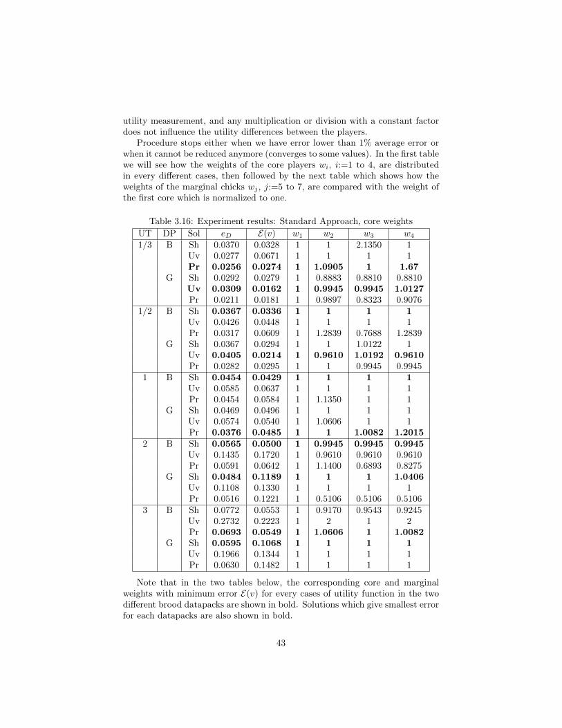
utility measurement, and any multiplication or division with a constant factordoes not influence the utility differences between the players.

Procedure stops either when we have error lower than 1% average error orwhen it cannot be reduced anymore (converges to some values). In the first tablewe will see how the weights of the core players wi, i:=1 to 4, are distributedin every different cases, then followed by the next table which shows how theweights of the marginal chicks wj , j:=5 to 7, are compared with the weight ofthe first core which is normalized to one.

Table 3.16: Experiment results: Standard Approach, core weights

UT DP Sol eD E(v) w1 w2 w3 w4

1/3 B Sh 0.0370 0.0328 1 1 2.1350 1Uv 0.0277 0.0671 1 1 1 1Pr 0.0256 0.0274 1 1.0905 1 1.67

G Sh 0.0292 0.0279 1 0.8883 0.8810 0.8810Uv 0.0309 0.0162 1 0.9945 0.9945 1.0127Pr 0.0211 0.0181 1 0.9897 0.8323 0.9076

1/2 B Sh 0.0367 0.0336 1 1 1 1Uv 0.0426 0.0448 1 1 1 1Pr 0.0317 0.0609 1 1.2839 0.7688 1.2839

G Sh 0.0367 0.0294 1 1 1.0122 1Uv 0.0405 0.0214 1 0.9610 1.0192 0.9610Pr 0.0282 0.0295 1 1 0.9945 0.9945

1 B Sh 0.0454 0.0429 1 1 1 1Uv 0.0585 0.0637 1 1 1 1Pr 0.0454 0.0584 1 1.1350 1 1

G Sh 0.0469 0.0496 1 1 1 1Uv 0.0574 0.0540 1 1.0606 1 1Pr 0.0376 0.0485 1 1 1.0082 1.2015

2 B Sh 0.0565 0.0500 1 0.9945 0.9945 0.9945Uv 0.1435 0.1720 1 0.9610 0.9610 0.9610Pr 0.0591 0.0642 1 1.1400 0.6893 0.8275

G Sh 0.0484 0.1189 1 1 1 1.0406Uv 0.1108 0.1330 1 1 1 1Pr 0.0516 0.1221 1 0.5106 0.5106 0.5106

3 B Sh 0.0772 0.0553 1 0.9170 0.9543 0.9245Uv 0.2732 0.2223 1 2 1 2Pr 0.0693 0.0549 1 1.0606 1 1.0082

G Sh 0.0595 0.1068 1 1 1 1Uv 0.1966 0.1344 1 1 1 1Pr 0.0630 0.1482 1 1 1 1

Note that in the two tables below, the corresponding core and marginalweights with minimum error E(v) for every cases of utility function in the twodifferent brood datapacks are shown in bold. Solutions which give smallest errorfor each datapacks are also shown in bold.

43

Table 3.17: Experiment results: Standard Approach, marginal weights

UT DP Sol eD E(v) w1 w5 w6 w7

1/3 B Sh 0.0370 0.0328 1 1.6700 2.1350 1.5894Uv 0.0277 0.0671 1 2 3 3Pr 0.0256 0.0274 1 1 2 4.6700

G Sh 0.0292 0.0279 1 1.1288 1.9891 0.9945Uv 0.0309 0.0162 1 0.9829 1.0894 1.8439Pr 0.0211 0.0181 1 1.4713 1.7621 3.6039

1/2 B Sh 0.0367 0.0336 1 2.0606 2.1294 1.0606Uv 0.0426 0.0448 1 2.0182 1 1Pr 0.0317 0.0609 1 1.5376 4.3203 2.1851

G Sh 0.0367 0.0294 1 1.0479 1.9220 0.9610Uv 0.0405 0.0214 1 2.0272 3.3362 1Pr 0.0282 0.0295 1 0.9945 1.9891 1.3018

1 B Sh 0.0454 0.0429 1 3 3.0905 1.0055Uv 0.0585 0.0637 1 2 3.0354 1.0606Pr 0.0454 0.0584 1 2.0082 1.0082 2.0182

G Sh 0.0469 0.0496 1 1.2621 3.6882 1Uv 0.0574 0.0540 1 3.0082 3.0406 3.1350Pr 0.0376 0.0485 1 2.1472 2.0406 1

2 B Sh 0.0565 0.0500 1 3.0240 2.9891 3.9782Uv 0.1435 0.1720 1 1.2533 2.0480 2.3587Pr 0.0591 0.0642 1 2.1936 0.9610 1.0390

G Sh 0.0484 0.1189 1 3 8.0606 4Uv 0.1108 0.1330 1 0.7708 3.3239 4.6563Pr 0.0516 0.1221 1 2.6782 2 1.1350

3 B Sh 0.0772 0.0553 1 1.1350 2.1622 1.8050Uv 0.2732 0.2223 1 1.9579 4.7700 1.8341Pr 0.0693 0.0549 1 2 1 3

G Sh 0.0595 0.1068 1 3 5.1350 1.2015Uv 0.1966 0.1344 1 2 1 1Pr 0.0630 0.1482 1 3.1405 3.7161 1

If we compare the results between each utility translation for both datapacks,we can clearly see that the concave translations (esp. p1/3) give the smallestminimum overall error E(v), thus is supporting our argument that concavity fitsbest with this brood data.

Taking the smallest minimum overall error E(v) of the bad years data B,which is 0.0274= 2.74% given by the Prenucleolus solution, we arrive at thesecore weights wi=(1, 1.0905, 1, 1.67) for each core chicks i=1 to 4, and marginalweights wj=(1, 2, 4.6700) for each marginals j=5 to 7 respectively, assumingthat the weight of the first core w1 is set to one. For the good years datawith the smallest minimum overall error E(v) of 0.0162=1.62% (given by thePrenucleolus solution), we get these weights wi=(1, 0.9945, 0.9945, 1.0127) for

44

each core chicks i=1 to 4 and wj=(0.9829, 1.0894, 1.8439) for each marginalsj=5 to 7.

Restricted Approach, Good and Bad years

We now apply the restricted approach R into our procedure and conduct anotherthirty experiments using this approach. Below are the result of the experiments,showing all the corresponding weights of the core and the marginal chicks foreach different cases of brood datapacks. Note that the cases with minimumerror E(v) for each datapack are shown in bold.

Table 3.18: Experiment results: Restricted Approach, core weights

UT DP Sol eD E(v) w1 w2 w3 w4

1/3 B Sh 0.0303 0.0156 1 1.0409 0.9420 1.8341Uv 0.0328 0.0164 1 1.3089 1.6700 1.0082Pr 0.0222 0.0184 1 1.0905 1 1.8172

G Sh 0.0256 0.0196 1 1.1134 0.9600 3.5387Uv 0.0248 0.0235 1 1.3008 1.0122 2.2867Pr 0.0301 0.0223 1 1 2.1194 1.1212

1/2 B Sh 0.0263 0.0245 1 1 1.2015 4Uv 0.0424 0.0278 1 1 2.0678 1Pr 0.0368 0.0271 1 1 1.8897 1.2920

G Sh 0.0353 0.0317 1 1.4489 2.6298 6.3283Uv 0.0371 0.0355 1 1.4713 1.1460 4.2077Pr 0.0344 0.0316 1 1 1 4.0488

1 B Sh 0.0600 0.0387 1 3.0100 2.5211 1.0272Uv 0.0531 0.0430 1 1.5000 1.5675 0.5000Pr 0.0396 0.0367 1 1 1 3.5811

G Sh 0.0582 0.0445 1 0.3851 0.3851 0.5009Uv 0.0423 0.0467 1 1.6700 1.0055 3.0612Pr 0.0535 0.0443 1 1 1 1.0788

2 B Sh 0.0486 0.0539 1 2 1 2.0905Uv 0.0741 0.0631 1 2 1 2.3512Pr 0.0792 0.0622 1 2.0000 1.0272 1.2015

G Sh 0.0599 0.0788 1 1.6700 2.6700 2Uv 0.0954 0.0872 1 1.3083 0.5222 0.5654Pr 0.0607 0.0639 1 1.2015 2 4.5023

3 B Sh 0.0360 0.0971 1 1.4489 1 1.2676Uv 0.0886 0.0994 1 1.1015 0.5269 1.5365Pr 0.1406 0.1056 1 1.5726 0.5237 2.0459

G Sh 0.1380 0.1147 1 1 1 1.0177Uv 0.1143 0.1449 1 0.3620 0.3190 0.3449Pr 0.0746 0.1548 1 0.5379 0.4933 0.4960

45

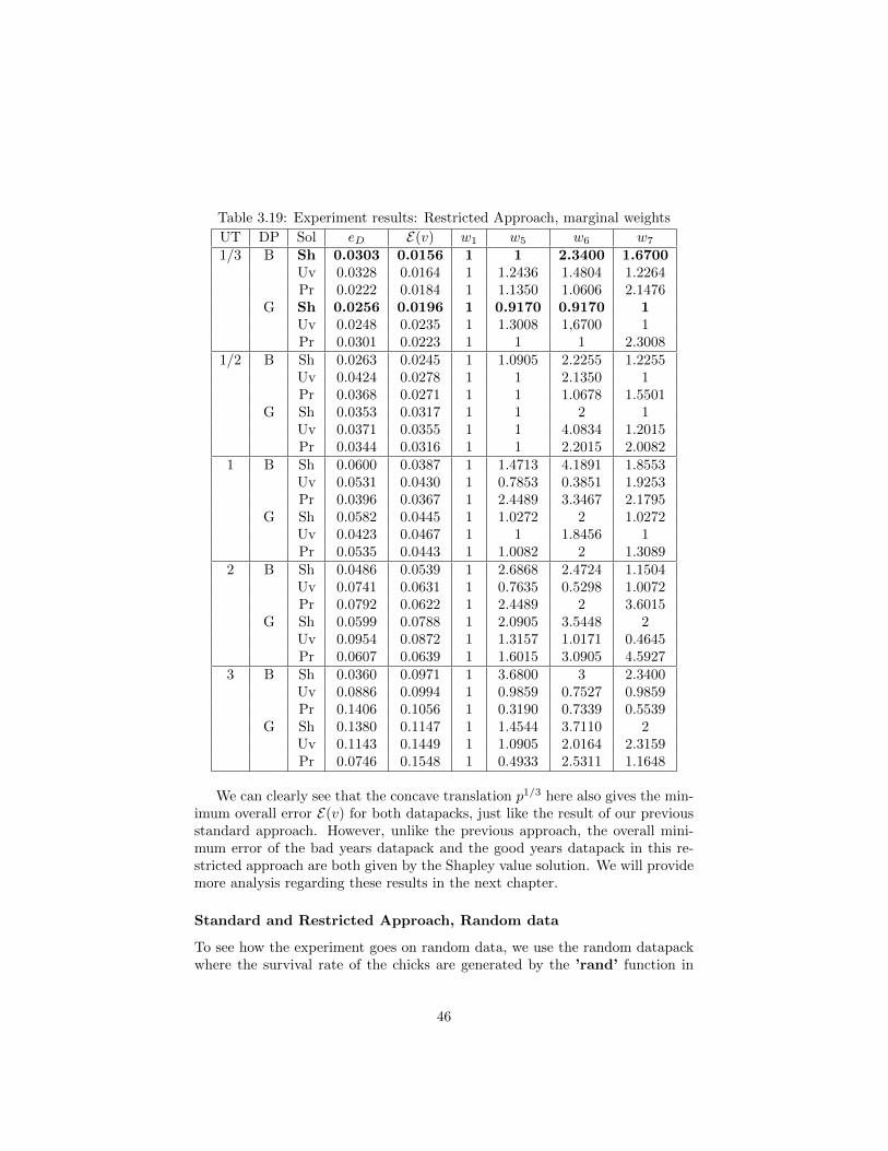
Table 3.19: Experiment results: Restricted Approach, marginal weights

UT DP Sol eD E(v) w1 w5 w6 w7

1/3 B Sh 0.0303 0.0156 1 1 2.3400 1.6700Uv 0.0328 0.0164 1 1.2436 1.4804 1.2264Pr 0.0222 0.0184 1 1.1350 1.0606 2.1476

G Sh 0.0256 0.0196 1 0.9170 0.9170 1Uv 0.0248 0.0235 1 1.3008 1,6700 1Pr 0.0301 0.0223 1 1 1 2.3008

1/2 B Sh 0.0263 0.0245 1 1.0905 2.2255 1.2255Uv 0.0424 0.0278 1 1 2.1350 1Pr 0.0368 0.0271 1 1 1.0678 1.5501

G Sh 0.0353 0.0317 1 1 2 1Uv 0.0371 0.0355 1 1 4.0834 1.2015Pr 0.0344 0.0316 1 1 2.2015 2.0082

1 B Sh 0.0600 0.0387 1 1.4713 4.1891 1.8553Uv 0.0531 0.0430 1 0.7853 0.3851 1.9253Pr 0.0396 0.0367 1 2.4489 3.3467 2.1795

G Sh 0.0582 0.0445 1 1.0272 2 1.0272Uv 0.0423 0.0467 1 1 1.8456 1Pr 0.0535 0.0443 1 1.0082 2 1.3089

2 B Sh 0.0486 0.0539 1 2.6868 2.4724 1.1504Uv 0.0741 0.0631 1 0.7635 0.5298 1.0072Pr 0.0792 0.0622 1 2.4489 2 3.6015

G Sh 0.0599 0.0788 1 2.0905 3.5448 2Uv 0.0954 0.0872 1 1.3157 1.0171 0.4645Pr 0.0607 0.0639 1 1.6015 3.0905 4.5927

3 B Sh 0.0360 0.0971 1 3.6800 3 2.3400Uv 0.0886 0.0994 1 0.9859 0.7527 0.9859Pr 0.1406 0.1056 1 0.3190 0.7339 0.5539

G Sh 0.1380 0.1147 1 1.4544 3.7110 2Uv 0.1143 0.1449 1 1.0905 2.0164 2.3159Pr 0.0746 0.1548 1 0.4933 2.5311 1.1648

We can clearly see that the concave translation p1/3 here also gives the min-imum overall error E(v) for both datapacks, just like the result of our previousstandard approach. However, unlike the previous approach, the overall mini-mum error of the bad years datapack and the good years datapack in this re-stricted approach are both given by the Shapley value solution. We will providemore analysis regarding these results in the next chapter.

Standard and Restricted Approach, Random data

To see how the experiment goes on random data, we use the random datapackwhere the survival rate of the chicks are generated by the ’rand’ function in

46

Matlab and are uniformly distributed in the interval [0,1]. The resulting errorsfor both approaches are shown in tables below:

Table 3.20: Experiment results: Standard Approach, random data

UT Sol E(v) eD1/3 Sh 0.0920 0.0862

Uv 0.1062 0.1309Pr 0.0762 0.0850

1/2 Sh 0.0242 0.06261Uv 0.0946 0.0934Pr 0.0215 0.0686

1 Sh 0.2101 0.1100Uv 0.2840 0.2337Pr 0.0725 0.0802

2 Sh 0.2555 0.2659Uv 0.7029 0.3539Pr 0.5768 0.3054

3 Sh 1.1263 0.3443Uv 13.1960 0.1501Pr 20.0752 0.3173

Table 3.21: Experiment results: Restricted Approach, random data

UT Sol E(v) eD1/3 Sh 0.0549 0.0690

Uv 0.1178 0.1003Pr 0.0726 0.0677

1/2 Sh 0.0560 0.0602Uv 0.1033 0.0849Pr 0.0718 0.0344

1 Sh 0.3683 0.1152Uv 0.6478 0.2361Pr 0.1618 0.1511

2 Sh 4.8517 0.2181Uv 15.9842 0.3801Pr 3.8706 0.2544

3 Sh 0.6727 0.2697Uv 0.4723 0.4718Pr 0.6913 0.2260

As shown in bold, we can easily see from Table 3.20 and 3.21 above that theoverall minimum errors on the random data hit below 5% in only two cases ofthe standard approach, and never on the restricted approach. As a result, theweights of the chicks on the random data become none of our interest since thetwo errors E(v) and eD are quite high in most of the cases.

47

Looking closely at the error E(v), notice that a different tendency appears inthese random dataset solutions compare to the brood datasets. The minimumE(v) error for the standard approach is achieved by p1/2 translation using thePrenucleolus solution, with error of 0.0215=2.15%, followed by the Shapleyvalue with error of 0.0242=2.42%. While the Utopia value solution seems tohave larger error with minimum of 0.0946=9.46%.

For the restricted approach, the concave utility function of p1/3 gives thesmallest error E(v) using the Shapley value solution with error of 0.0549=5.49%.However, this error is probably still quite large for the result to be consideredas a best fit.

In general, unlike the brood datapacks which has smallest minimum E(v)error under the p1/3 translation, both approaches on the random data givequite a high error under this p1/3 translation, ranging from 5.5% to 12%.

Interestingly, we can also highlight on the largest minimum E(v) error forthe standard approach which is given by the Prenucleolus solution under theconvex p3 translation, with 20.0752=2007.52% of overall error. While for therestricted approach, the largest minimum E(v) error is achieved by the Utopiasolution with a convex p2 translation, resulting 15.9842=1598% of error. Bothare naturally unacceptable. Therefore, we cannot say that the random data fitsany solution concepts mentioned in this thesis.

Note that in the first experiment with no restriction, we want to see whetherwe can achieve smaller error below 1%. However, this never occurs in any ofthe 90 experiments above; none of them stops at the 1% average of error.

3.3 Validation

When finding the best weight system using the standard approach, we validatethe resulting weights of the core chicks by taking a general direction instead of apredetermined one. Doing this will allow us to see if by any chance, the weightsof the core chicks will be the same or at least close to each other. Indeed, wefound from Table 3.16 and Table 3.18 that in almost all cases where the error issmall, the weights of the other core chicks appear to be the same as the weightof the first core chick, which we set to be equal to one. While in most caseswhere the error is quite small, the weights of the core chicks are close to one;i.e. almost the same with the weight of the first core.

Once, we had an experience with some strange results. The resulting weightsof the prenucleolus and the utopia solution concepts are not ’going in the samedirection’ as the results from our Shapley value solution: in any cases of thebrood data, almost all weights of the marginal broods are smaller than theweight of the core. Logically, the weights of the marginals will usually be largerthan the core as a results of parental favoritism where food is valued moreby the marginals rather than the core (see subsection 3.2.2 for the detailedexplanation).

In order to validate, we run our ’old’ codes which is made only for fitting thegame using the Shapley value solution concept (see [18] for different versions of

48

these fitting procedures), indeed we got the same tendency with our Shapleyvalue results: the weights of the marginals are almost always larger than thecore. Therefore, we check and correct our codes for the prenucleolus and utopiasolutions by adapting the same procedure with the Shapley value. Now ourresults for all the approaches seem to be more convincing as the marginal weightshave larger weights in most of the cases.

49

Chapter 4

Further Analysis

This chapter considers the analysis of the results from computational and bio-logical point of view, to see which properties seem to play a major role in thebrood data and which known solution concept fits best with the brood data.

4.1 Notations

To be able to read the tables mentioned in the analysis of this chapter, herewe provide again the same notations as we use in the previous chapter. Apprdenotes the modeling approach we are using, S for the Standard approach andR for the Restricted approach. DP denotes which datapack we are taking intoaccount, B for the Bad years data, G for the Good years data, and Rd for theRandom data. Notation Sol denotes what kind of solution concept we choose,Sh for the Shapley value, Uv for the Utopia value, and Pr for the Prenucleolus.Notation UT denotes which utility translation we are considering, either p1/3,p1/2, p1, p2, or p3. Notation E(v) denotes the minimum overall error, whichexpress how well the data fits the new fitted game, while eD denotes the errorwith respect to the data, expressing how well the game solutions fit the data.

4.2 Findings and Reasoning

We divide the findings we got from the experiments into seven different types ofanalysis, and explain the details of the analysis in seven different sections below.We will also give some reasonable arguments behind the results we found in theexperiments.

4.2.1 Smallest Error vs Utility Translation

As we have known from the results of our experiments in the previous chapter,smallest errors are reached by the concave p1/3 translation in all cases of thebrood data solutions with two different modeling approaches. Thus, we may

50

already say that the brood survival rate data in our case is better translatedwith concavity of p1/3. For a clear comparison on the minimum overall error forevery different cases of utility translations, see the table below. Note that theminimum overall error for two different approaches and datapacks are shown inbold.

Table 4.1: Smallest Error vs Utility Translation

E(v)Appr DP Sol p1/3 p1/2 p1 p2 p3

S B Sh 0.0328 0.0336 0.0429 0.0500 0.0553Uv 0.0671 0.0448 0.0637 0.1720 0.2223Pr 0.0274 0.0609 0.0584 0.0642 0.0549

G Sh 0.0279 0.0294 0.0496 0.1189 0.1068Uv 0.0162 0.0214 0.0540 0.1330 0.1344Pr 0.0181 0.0295 0.0485 0.1221 0.1482

R B Sh 0.0156 0.0245 0.0387 0.0539 0.0971Uv 0.0164 0.0278 0.0430 0.0631 0.0994Pr 0.0184 0.0271 0.0367 0.0622 0.1056

G Sh 0.0196 0.0317 0.0445 0.0788 0.1147Uv 0.0235 0.0355 0.0467 0.0872 0.1449Pr 0.0223 0.0316 0.0443 0.0639 0.1548

We can see from the table that the convex translation p2 hit 5% overall erroronly once with the Shapley value solution concept, and never with the othersolution concepts. While in the convex p3 translation, the minimum overallerror is always above 5% for any solution concepts.

Taking a close look into the results using the Shapley value solution conceptin the table above, we may notice that the more concave the utility translationpa (a = 1/3, 1/2, 1, 2, 3) is, the smaller the error. For the Utopia value andthe Prenucleolus solutions, sometimes the concave p1/2 translation gives smallererror than the concave p1/3 translation. However, concave translations in generalalways give smaller error than the convex ones.

Why concave translation fits best? As we have argued before in the previouschapter, if the food allocation for the marginal chick is increased a little bit more,for example from 0.3 to 0.4 gram, the chick’s probability of survive will increasea lot more, and it might even save them from dying. While if the core chick’ssurvival rate is already high, there is almost no difference if it is being fed alittle bit more; in any chance, most probably it will survive. In other words,the food is considered to be more valuable for the marginals rather than for thecore. This may explains why the concave translation fits best than the convexone.

4.2.2 Smallest Error vs Solution

The smallest overall error for the good years and the bad years data in thestandard approach are given by the Utopia value and the Prenucleolus solutions,

51

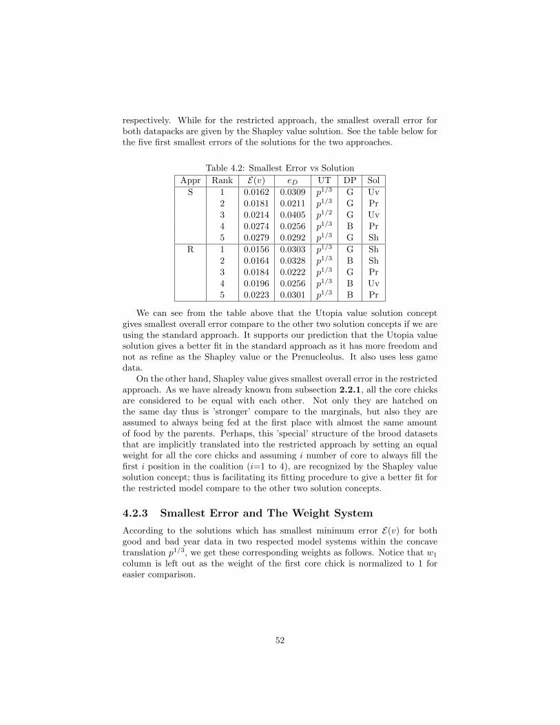
respectively. While for the restricted approach, the smallest overall error forboth datapacks are given by the Shapley value solution. See the table below forthe five first smallest errors of the solutions for the two approaches.

Table 4.2: Smallest Error vs Solution

Appr Rank E(v) eD UT DP Sol

S 1 0.0162 0.0309 p1/3 G Uv2 0.0181 0.0211 p1/3 G Pr3 0.0214 0.0405 p1/2 G Uv4 0.0274 0.0256 p1/3 B Pr5 0.0279 0.0292 p1/3 G Sh

R 1 0.0156 0.0303 p1/3 G Sh2 0.0164 0.0328 p1/3 B Sh3 0.0184 0.0222 p1/3 G Pr4 0.0196 0.0256 p1/3 B Uv5 0.0223 0.0301 p1/3 B Pr

We can see from the table above that the Utopia value solution conceptgives smallest overall error compare to the other two solution concepts if we areusing the standard approach. It supports our prediction that the Utopia valuesolution gives a better fit in the standard approach as it has more freedom andnot as refine as the Shapley value or the Prenucleolus. It also uses less gamedata.

On the other hand, Shapley value gives smallest overall error in the restrictedapproach. As we have already known from subsection 2.2.1, all the core chicksare considered to be equal with each other. Not only they are hatched onthe same day thus is ’stronger’ compare to the marginals, but also they areassumed to always being fed at the first place with almost the same amountof food by the parents. Perhaps, this ’special’ structure of the brood datasetsthat are implicitly translated into the restricted approach by setting an equalweight for all the core chicks and assuming i number of core to always fill thefirst i position in the coalition (i=1 to 4), are recognized by the Shapley valuesolution concept; thus is facilitating its fitting procedure to give a better fit forthe restricted model compare to the other two solution concepts.

4.2.3 Smallest Error and The Weight System

According to the solutions which has smallest minimum error E(v) for bothgood and bad year data in two respected model systems within the concavetranslation p1/3, we get these corresponding weights as follows. Notice that w1

column is left out as the weight of the first core chick is normalized to 1 foreasier comparison.

52

Table 4.3: Smallest Error and The Weight System

Appr DP E(v) eD w2 w3 w4 w5 w6 w7

S B 0.0274 0.0256 1.09 1 1.67 1.67 2.14 1.59G 0.0162 0.0309 0.99 0.99 1.01 1.13 1.99 0.99

R B 0.0164 0.0328 1.31 1.67 1.01 1 2.34 1.67G 0.0156 0.0303 1.04 0.94 1.83 0.92 0.92 1

What we want to see is whether the weights of all core chicks will be thesame (i.e. close to each other), at least in the standard approach where weallow anonimity between the core chicks. By dividing all the weights of theother chicks using the weight of the first core chick, we see that almost allthe other core weights are very close to 1 in the standard approach with thesmallest error. Interestingly, this is also the case for the restricted approach.Even though the first four players do not take similar position in the game,we see that similar assumption seems to hold for the restricted case, especiallywhen the error is small: the weights of the other core chicks are most of thetime close enough to 1.

However, we may see some unexpected values appearing on the weight of thecore and the marginal broods: some weights of the core chicks appear to be quitelarger than one, and some weights of the marginal chicks are a little bit smallerthan one. This is due to the fact that our search procedure is not ’perfect’.During the fitting of the weight, sometimes we end up in a local optima andthe procedure does not allow us to search further to find the best fit. Given thesearch procedure, we cannot do better. However, most of the time when erroris below 5%, this is usually not the case.

4.2.4 The Brood Data and The Weight System

Now we compare the weight system in different brood datapacks for the twoapproaches. We want to check whether the marginals have larger weights in thebad years compare to the good years, at least for the case where the averageerror is minimum. Note that the largest weights of the marginals are shown inbold.

Table 4.4: The Brood Data and The Weight System

Appr DP E(v) eD w5 w6 w7

S B 0.0274 0.0256 1.67 2.14 1.59G 0.0162 0.0309 1.13 1.99 0.99

R B 0.0164 0.0328 1 2.34 1.67G 0.0156 0.0303 0.92 0.92 1

We can easily see that in the case where the overall average error E(v) is min-imum, the marginal chicks have larger weights in the bad years rather than inthe good years. These results support our prediction that parental favoritismexists even worse during the bad years period.

53

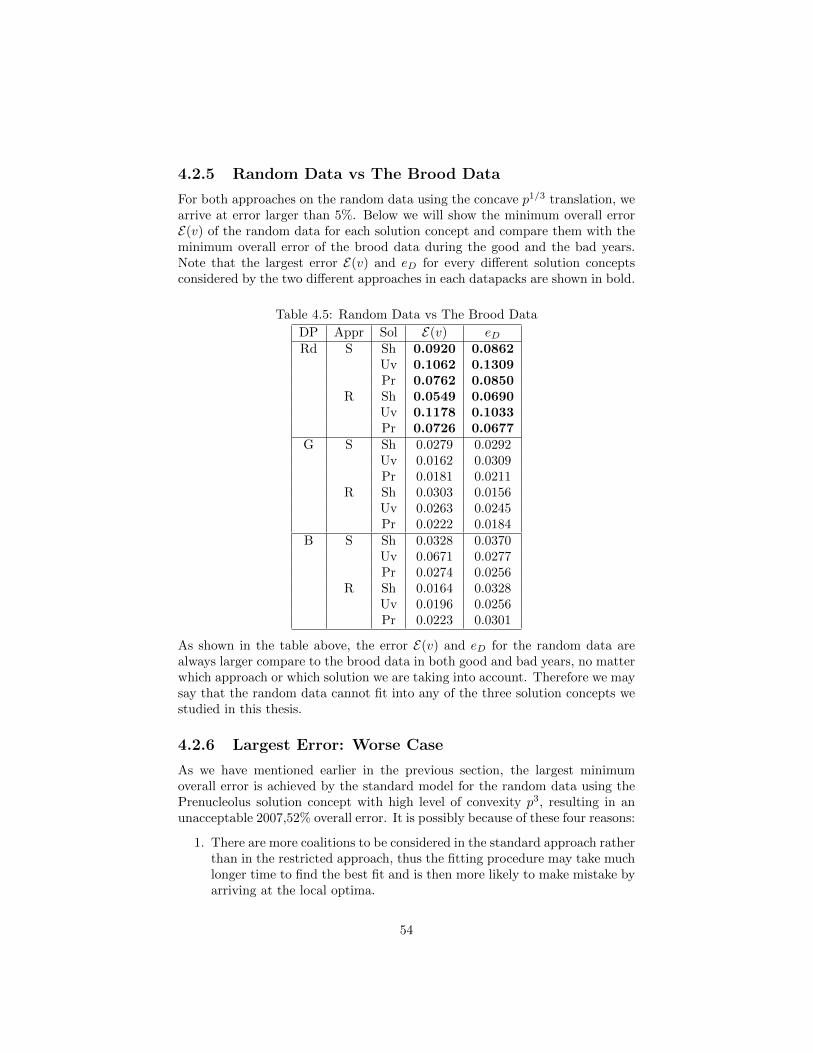
4.2.5 Random Data vs The Brood Data

For both approaches on the random data using the concave p1/3 translation, wearrive at error larger than 5%. Below we will show the minimum overall errorE(v) of the random data for each solution concept and compare them with theminimum overall error of the brood data during the good and the bad years.Note that the largest error E(v) and eD for every different solution conceptsconsidered by the two different approaches in each datapacks are shown in bold.

Table 4.5: Random Data vs The Brood Data

DP Appr Sol E(v) eDRd S Sh 0.0920 0.0862

Uv 0.1062 0.1309Pr 0.0762 0.0850

R Sh 0.0549 0.0690Uv 0.1178 0.1033Pr 0.0726 0.0677

G S Sh 0.0279 0.0292Uv 0.0162 0.0309Pr 0.0181 0.0211

R Sh 0.0303 0.0156Uv 0.0263 0.0245Pr 0.0222 0.0184

B S Sh 0.0328 0.0370Uv 0.0671 0.0277Pr 0.0274 0.0256

R Sh 0.0164 0.0328Uv 0.0196 0.0256Pr 0.0223 0.0301

As shown in the table above, the error E(v) and eD for the random data arealways larger compare to the brood data in both good and bad years, no matterwhich approach or which solution we are taking into account. Therefore we maysay that the random data cannot fit into any of the three solution concepts westudied in this thesis.

4.2.6 Largest Error: Worse Case

As we have mentioned earlier in the previous section, the largest minimumoverall error is achieved by the standard model for the random data using thePrenucleolus solution concept with high level of convexity p3, resulting in anunacceptable 2007,52% overall error. It is possibly because of these four reasons:

1. There are more coalitions to be considered in the standard approach ratherthan in the restricted approach, thus the fitting procedure may take muchlonger time to find the best fit and is then more likely to make mistake byarriving at the local optima.

54

2. It is hard to fit the random data since there is no specific structure, un-like the brood datasets which have some ’special’ properties that can becaptured by some of the solution concepts.

3. The Prenucleolus solution concept itself contains a lot of sophisticated tun-ing and balancing, unlike the Utopia value or the Shapley value solutionswhich have the additivity property that enables a fast fitting.

4. The utility translation is convex instead of concave; in which we alreadyprove that concave translations pa, a = 1/3, 1/2, usually give smallerminimum overall error E(v) rather than the convex translation pa, a =2, 3 or the linear case without translations.

4.2.7 Time Consumption

As an addition to the analysis, below we will show the largest time consumptionfor every solution concept in each brood datapack which we have not mention inthe previous chapter. Note that the two largest time consumptions (in seconds),each corresponds to the standard and the restricted approach, are shown in bold.

Table 4.6: Time Consumptions

Appr DP Sol UT timeS B Sh 3 596,6758815

Uv 1/2 1258,745863Pr 1 5482,497638

G Sh 2 1433,950145Uv 1 5436,586818Pr 1/3 6133,127812

R B Sh 1/2 6294,65302Uv 1/3 1433,452379Pr 2 4525,036143

G Sh 1 109,2940425Uv 2 4140,893783Pr 1/2 6470,758277

We see that the largest time consumptions in both approaches happen when weconsider the Prenucleolus solution, especially under the concave translations.

As an insight on the time consumption of the experiments, fitting usingthe Prenucleolus solution concept is much slower compare to the other solutionconcepts perhaps because the Prenucleolus does not have special properties likelinearity that can be explored in the implementation of the fitting procedure.

55

Chapter 5

Final Conclusion

In this last chapter we provide conclusions and future works of our research.

5.1 Conclusions

As Forbes (2011) said in his paper [16], survival to leave the nest is a usefulproxy to measure the evolutionary fitness. It shows a range of variation, fromthe virtually guaranteed survival of core offspring in small broods, to the nearcertain death of marginal offspring in large broods. Knowing the importance ofthis survival rate for the blackbird chicks, we conclude our research as follows:

• The modeling and calculation choices we made using the Shapley valuesolution concept have proved that parental favoritism does exist in mostcases of the brood data, especially during the bad years period.

• In general, property such as linearity in the Shapley value solution allowsa fast fitting in the brood data. The restricted structure of the brooddatasets also enables the Shapley value solution concept to give a reason-able fit within a reasonable time.

• Prenucleolus solution results are shown in various kind of experiments,perhaps because of the fact that it is a high profile solution where there arequite a lot of balancing in the procedure, i.e. fine tuning is sophisticated.

• If we want a simple, ’quick and dirty’ solution which also enable fastfitting with quite feasible solution, then Utopia value solution concept canbe considered as a choice.

• Whatever model of the brood data we are taking, the results of the ex-periments have some tendencies:

1. The weights of the marginals are usually larger than the cores, sincethe food is valued more by the marginals as a result of parentalfavoritism.

56

2. The concavity translations fit best as our brood data is not linear.Small increase on the food allocation for the marginals could increasethe chick’s probability of survive a lot more, while giving more foodto the core chick who already has a high survival rate does not give adifferent output as the core already has a great chance of surviving.

• The worst case of error is achieved by the standard model for the randomdata using the Prenucleolus solution concept with high level of convexityp3. Thus, the more complex the model, the harder it fits.

• To summarize the results of the experiments, we can say that the moreconcave the utility translation, the smaller the error, the better the gamefits the solutions, the more we can trust the resulting weight system.

Finally we conclude that we have been able to implement the Shapley valuesolution concept to tackle the bird brood food allocation problem, and compareits result with the other known solution concepts namely the Utopia value andthe Prenucleolus.

We also successfully translate the biological problem of blackbird food al-location into a cooperative game approach using various techniques known inliterature.

5.2 Future Works

Given a vast amount of brood data as well as a vast amount of results fromthe experiments, there are still a lot to be investigated further in this research.One can really discriminate among the approaches, the solutions, the utilityfunctions, and the datapacks that are used, and analyze the results for eachexperiment.

To get a better understanding, one might also change the solution conceptand examine the effects in the current situation. To some extent, we adaptedthe anonimity property of the Shapley value by applying weights. What willhappen if we furthermore play around with the dummy player property, or whenwe allow for restricted cooperation settings, as are seen in the Utopia value. Inall these cases we may arrive at more weight in the importance of the gamesolution properties in the interpretation of the data.

The fitting procedure may also be tuned in a different way. The appliedsettings were tuned only briefly and only in the Shapley value application. Amore sophisticated calibration might enable a fitting with smaller erroors, andthus with more reliable conclusions.

57

Bibliography

[1] S. Forbes, A Natural History of Families, Princeton University Press, 9May 2005

[2] S. Forbes, ”Sibling Symbiosis in Nestling Birds”, Auk 124, pp. 1-10, 2007

[3] A. Kacelnik, et al, ”Food allocation among nestling starlings: sibling com-petition and the scope of parental choice”, in The Royal Society B, Bio-logical Sciences, (London, U.K.), vol. 259, no. 1356, pp. 259-263, 22 March1995

[4] V.F. Hendricks and P.G. Hansen, ”Game The-ory: 5 Questions”, Automatic Press/VIP, April 2007http://www.gametheorists.com/Interviews/young.html

[5] C-J. Haake, A. Kashiwada, and F.E. Su, ”The Shapley value of phyloge-netic trees”, working papers, Bielefeld University, Institute of MathematicalEconomics, 2005, http://EconPapers.repec.org/RePEc:bie:wpaper:363

[6] E. Binenbaum and P.G. Pardey, ”Collective Action in Plant Breed-ing”, in Proc. 2005 annual meeting, Providence, RI, AmericanAgricultural Economics Association (New Name 2008: Agriculturaland Applied Economics Association), no. 19530, 24-27 July 2005,http://EconPapers.repec.org/RePEc:ags:aaea05:19530

[7] P. Pintassilgo, ”The New Member Problem in the Cooperative Man-agement of the Northern Atlantic Bluefin Tuna”, FEUNL Working Pa-per Series, Universidade Nova de Lisboa, Faculdade de Economia, 2000,http://EconPapers.repec.org/RePEc:unl:unlfep:wp373

[8] A. Torkaman, N.M. Charkari, and M. Aghaeipour, ”An approach forleukemia classification based on cooperative game theory”, Anal CellPathol, (Amsterdam, The Netherlands), vol. 34, no. 5, pp. 235-46, 2011

[9] F. Thuijsman, ”To play and to share; a brief introduction to game theory”,lecture notes, Maastricht University, Department of Knowledge Engineer-ing, 2011

58

[10] R.J. Aumann and M. Maschler, ”Game Theoretic Analysis of a BankruptcyProblem from the Talmud”, Journal of Economic Theory, no. 36, pp. 195-213, 1985

[11] A. Kar, M. Mitra, and S. Mutuswami, ”On the coincidence of the prenucle-olus and the Shapley value”, Mathematical Social Sciences, Elsevier, vol.57, no. 1, pp. 16-25, January 2009

[12] J. Derks, ”A cooperative game approach to the analysis of allocation se-quences”, discussion notes, Maastricht University, Department of Knowl-edge Engineering, 26 September 2008

[13] H. Wiese, ”Applied cooperative game theory: Dividends”, lecture notes,University of Leipzig, April 2010

[14] J.J.M. Derks and H.H. Haller, ”Weighted Nucleoli”, International Journalof Game Theory, no. 28, pp. 173-188, 1999

[15] J. Oswald, J. Derks, and H. Peters, ”Prenucleolus and Nucleolus of a Coop-erative Game: Characterizations by Tight Coalitions”, in Proc. 3rd Inter-national Conference on Approximation and Optimization in the Caribbean,(Puebla, Mexico), 8-13 October 1995

[16] S. Forbes, ”Parental preference for investment risk incites family strife”,Journal of Bioeconomics, Springer, (Netherlands), vol. 14(2), pp. 115-128,1 July 2012, http://dx.doi.org/10.1007/s10818-011-9122-0

[17] T.S. Ferguson, ”Game Theory”, electronic text, UCLA, Mathematics De-partment, 2008

[18] J. Derks, ”Cooperative Game Fitting Procedures”, Matlab toolbox pack-age, April 2012

[19] A.Ph. Rosenbusch, ”Fairness Considerations in Cooperative Games”, lec-ture notes, TU Darmstadt, Department of Mathematics, April 2011,http://tuprints.ulb.tu-darmstadt.de/2573/

[20] H. Keiding, ”Solution concepts for TU games: The τ -value”, lecturenotes, University of Copenhagen, Department of Economics, pp. 1-4,http://www.econ.ku.dk/keiding/underv/GameTheory/tijsrevEng.pdf

[21] S. Brnzei, ”State of the Art: Solution Concepts for Coalitional Games”,BRAIN (Broad Research in Artificial Intelligence and Neuroscience), vol.1, no. 2, University of Waterloo, David R. Cheriton School of ComputerScience, 2010

[22] M.J. Osborne, ”Mathematical methods for economic theory: a tutorial”,electronic tutorial, University of Toronto, Department of Economics, 28November 2011

59

[23] L.S. Shapley, A Value for n-Person Games, ”In Contributions to the Theoryof Games”, Annals of Mathematics Studies, vol. II, no. 28, pp. 307-317,H.W. Kuhn and A.W. Tucker, eds., Princeton University Press, 1953

[24] D. Schmeidler, ”The nucleolus of a characteristic function form game”, De-fense Technical Information Center, pp. 1-13, Hebrew University Jerusalem(Israel), Department of Mathematics, 1966

[25] J.J.M. Derks and H.M. Peters, ”Orderings, Excess Functions, and the Nu-cleolus”, Mathematical Social Sciences, no. 36, pp. 175-182, 1998

[26] R.v.d. Brink, ”Balanced consistency and balanced cost reduction for se-quencing problems”, Social Choice and Welfare, Springer-Verlag, vol. 38,no. 3, pp. 519-529, March 2012, http://dx.doi.org/10.1007/s00355-011-0533-6

[27] D. Monderer, D. Samet, and L.S. Shapley, ”Weighted Values and the Core”,International Journal of Game Theory, vol. 21, pp. 27-39, 1992

60