mastering excelimages.ruceci.com/pdfs/wtexfbook.pdf · · 2016-09-14mastering excel® functions...

Mastering Excel®

Functions & Formulas

© 2016 SkillPatha division of the Graceland College Center for Professional Development and Lifelong Learning, Inc.All rights reserved, including the right to reproduce this material or any part thereof in any manner.

Financial and Statistical Function Overview

Financial and Statistical Function Overview• Financial: PMT, FV, and RATE functions

• Statistical: AVERAGE, MAX, MIN, MODE, MEDIAN

• Others: STDEV, VAR, PERCENTILE, QUARTILE, RANK, LARGE

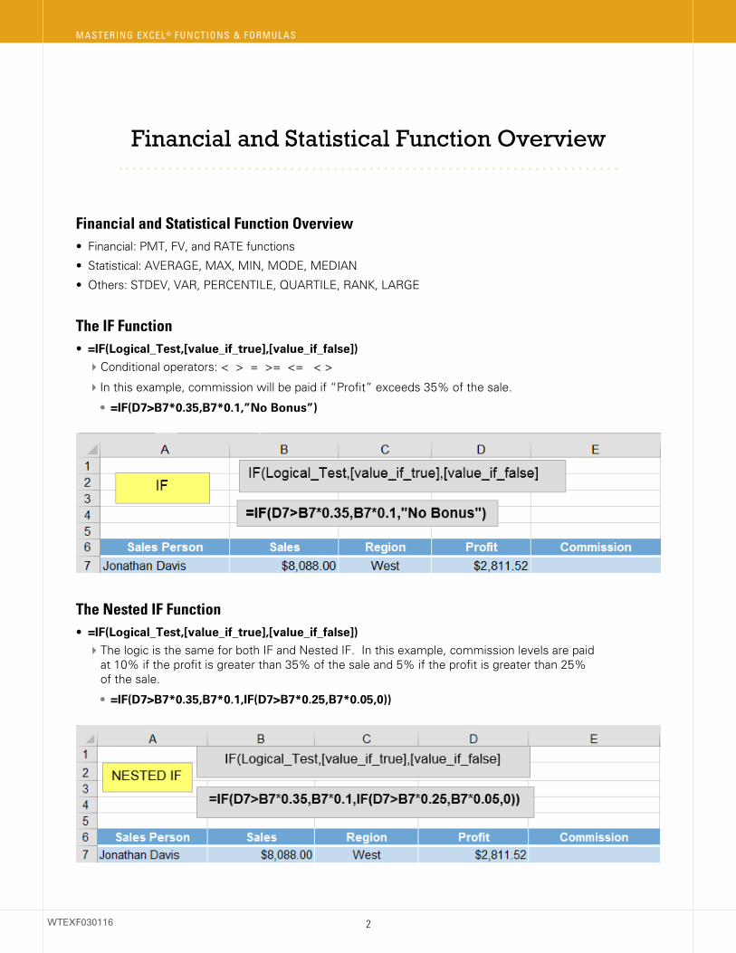
The IF Function• =IF(Logical_Test,[value_if_true],[value_if_false])

Conditional operators: < > = >= <= < >

In this example, commission will be paid if “Profit” exceeds 35% of the sale.

• =IF(D7>B7*0.35,B7*0.1,”No Bonus”)

The Nested IF Function• =IF(Logical_Test,[value_if_true],[value_if_false])

The logic is the same for both IF and Nested IF. In this example, commission levels are paid at 10% if the profit is greater than 35% of the sale and 5% if the profit is greater than 25% of the sale.

• =IF(D7>B7*0.35,B7*0.1,IF(D7>B7*0.25,B7*0.05,0))

2

MASTERING EXCEL ® FUNCTIONS & FORMULAS

WTEXF030116

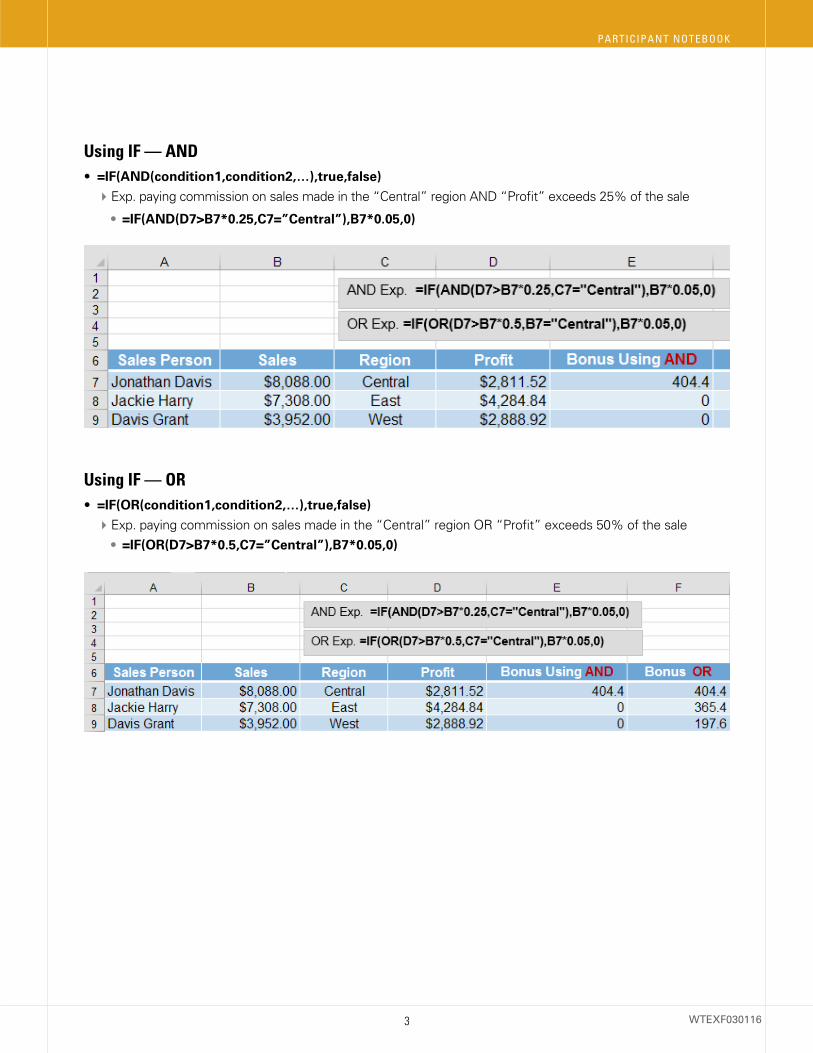
Using IF — AND• =IF(AND(condition1,condition2,…),true,false)

Exp. paying commission on sales made in the “Central” region AND “Profit” exceeds 25% of the sale

• =IF(AND(D7>B7*0.25,C7=”Central”),B7*0.05,0)

Using IF — OR• =IF(OR(condition1,condition2,…),true,false)

Exp. paying commission on sales made in the “Central” region OR “Profit” exceeds 50% of the sale • =IF(OR(D7>B7*0.5,C7=”Central”),B7*0.05,0)

3

PARTICIPANT NOTEBOOK

WTEXF030116

CHOOSEThe CHOOSE function allows you to insert data into a cell based on a table rather than having to manually insert the data.

The structure of the CHOOSE function is:

CHOOSE(index, value1, value2, value3…)

In this example, we are using CHOOSE to determine what level of award the salespeople receive based on their rank. This prevents us from having to manually determine the awards.

4


WTEXF030116

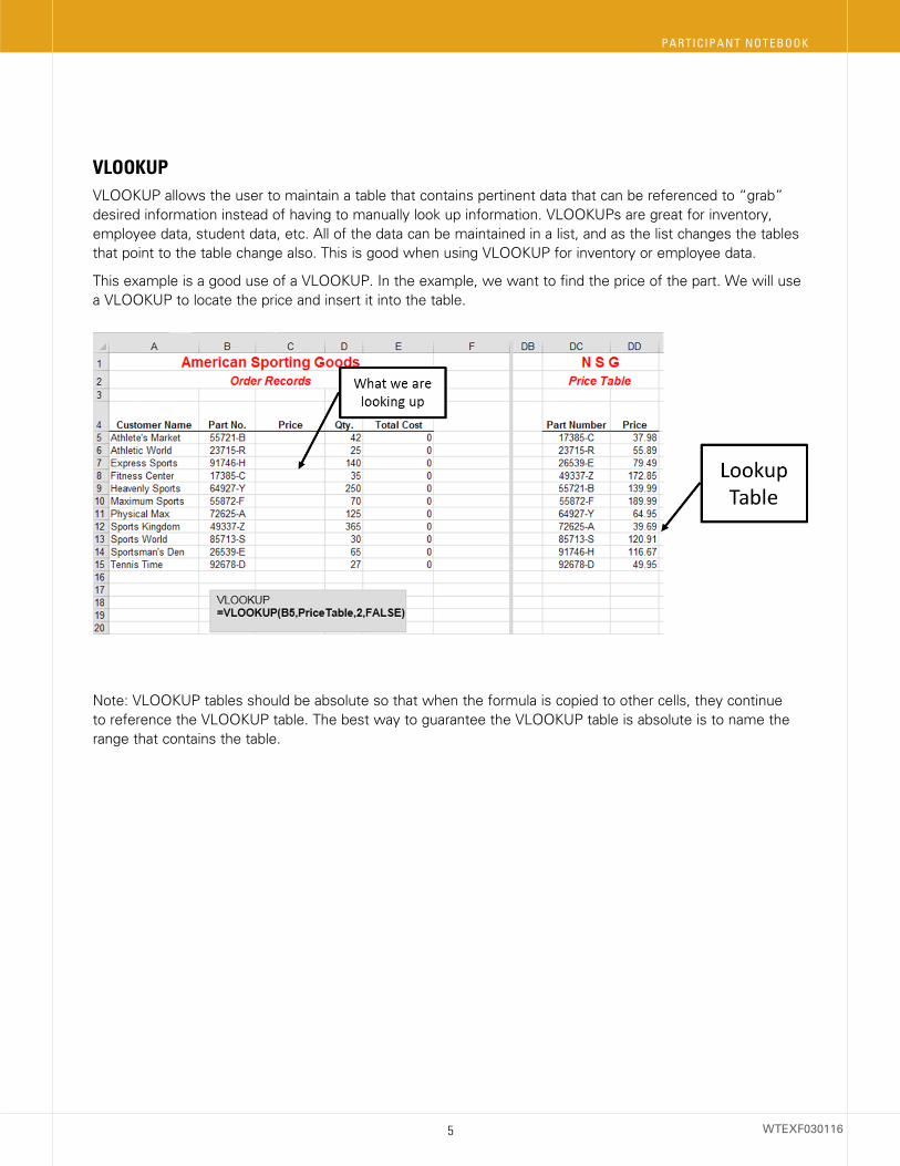
VLOOKUPVLOOKUP allows the user to maintain a table that contains pertinent data that can be referenced to “grab” desired information instead of having to manually look up information. VLOOKUPs are great for inventory, employee data, student data, etc. All of the data can be maintained in a list, and as the list changes the tables that point to the table change also. This is good when using VLOOKUP for inventory or employee data.

This example is a good use of a VLOOKUP. In the example, we want to find the price of the part. We will use a VLOOKUP to locate the price and insert it into the table.

Note: VLOOKUP tables should be absolute so that when the formula is copied to other cells, they continue to reference the VLOOKUP table. The best way to guarantee the VLOOKUP table is absolute is to name the range that contains the table.

5


WTEXF030116

The MATCH Function• MATCH Logic =MATCH(lookupValue,lookup_array,[matchType])

The MATCH function is used to find a specific position in a table array and returns a column or row number.

MATCH can be used to compare two lists to determine duplicate values, or new values. In the example below, MATCH was used to find returning students from one semester to the next. Two lists are being compared, and a row number will be returned where a match is found.

An IFERROR and IF statement were used to provide a text value of “RS” when a match was made, and “New Student” was returned when no match was found.

• =IFERROR(IF(MATCH(E4,$A$4:$A$12,0),”RS”),”NS”)

Match Type = 0

Returns the position in A4:A12 of the first value that exactly matches LookupValue

Values in the lookup table can be in any order.

Match Type = 1

Returns the position of the largest value in A4:A12 <= the LookupValue

Values in the lookup table must be in ascending order.

Match Type = -1

Returns the position of the smallest value in A4:A12 >= the LookupValue

Values in the lookup table must be in descending order.

6


WTEXF030116

The INDEX Function• =INDEX(array,row_number,column_Number)

• =INDEX(D3:M9,6,3) returns content of the cell at the intersection of the sixth row and third column of the range D3:M9.

Note: INDEX by itself is useful, but when combined with MATCH becomes very flexible.

INDEX and MATCH Together

• =INDEX(array,MATCH(lookup_value,lookup_array,[match_type]),[column_num])

• =INDEX(D2:M9,Match(A2,C2:C9,0),3)

• =INDEX(array, row_num,MATCH(lookupValue,Lookup_array, [matchType]))

• =INDEX(D2:M9,7,Match(A2,C2:C9,0))

Example: In the screen shot below, a value is interred in cell B15. The value in cell B15 is compared to a range of information in cells A4:A12. If a MATCH is found, a row number is given. To find the column number, a value is added to cell D15. This information is compared to the values shown in cells E3:K3. When an exact match is found, a column number is returned. Having both a row and column number, a weekly test score is displayed from the table D4:K12.

=INDEX(D4:K12,MATCH(D15,A4:A12,0),MATCH(B15,D3:K3,0))

7


WTEXF030116

Using COUNTIF and SUMIF

To count or sum a criteria range, use COUNTIF or SUMIF. In the example above, all sales that match the criteria are totaled. The name of the salesperson in Column M:M is compared to the names found in column B:B. When a match is found, the commission in column J:J is totaled and shown in the cell to the left of the name in column M:M

• SUMIF Logic =SUMIF(Range,Criteria,[SumRange])

• =SUMIF(B:B,F6,C:C)

Other COUNTIF and SUMIF Examples

• =COUNTIF(E2:E90,”=Colorado”) Counts how many cells in the range E2:E90 equal “Colorado”

• =COUNTIFS(E:E,”=Colorado”,G:G,100) Counts how often both entries in column E equal “Colorado” and column G = 100

• =SUMIF(K:K,”=Oregon”,J:J) Totals all column J values when the corresponding column K entry equals “Oregon”

• =SUMIFS(F:F,K:K,”=Ohio”,M:M,5) Totals all values in column F when the corresponding column K entry equals “Ohio” and the corresponding column M entry = 5

• =AVERAGEIF(K:K,”=Ohio”,J:J) Averages all column J values when the corresponding column K entry equals “Ohio”

• =AVERAGEIFS(F:F,K:K,”=Kentucky”,Q:Q,7) Averages all column F values when the corresponding column K entry equals “Kentucky” and the corresponding column Q entry = 7

8


WTEXF030116

Array Formulas

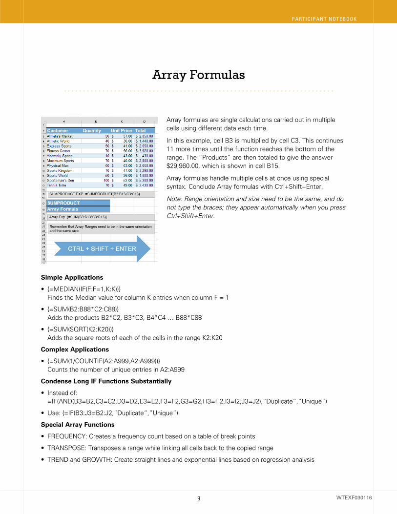
Array formulas are single calculations carried out in multiple cells using different data each time.

In this example, cell B3 is multiplied by cell C3. This continues 11 more times until the function reaches the bottom of the range. The “Products” are then totaled to give the answer $29,960.00, which is shown in cell B15.

Array formulas handle multiple cells at once using special syntax. Conclude Array formulas with Ctrl+Shift+Enter.

Note: Range orientation and size need to be the same, and do not type the braces; they appear automatically when you press Ctrl+Shift+Enter.

Simple Applications

• {=MEDIAN(IF(F:F=1,K:K))} Finds the Median value for column K entries when column F = 1

• {=SUM(B2:B88*C2:C88)} Adds the products B2*C2, B3*C3, B4*C4 … B88*C88

• {=SUM(SQRT(K2:K20))} Adds the square roots of each of the cells in the range K2:K20

Complex Applications

• {=SUM(1/COUNTIF(A2:A999,A2:A999))} Counts the number of unique entries in A2:A999

Condense Long IF Functions Substantially

• Instead of: =IF(AND(B3=B2,C3=C2,D3=D2,E3=E2,F3=F2,G3=G2,H3=H2,I3=I2,J3=J2),”Duplicate”,”Unique”)

• Use: {=IF(B3:J3=B2:J2,”Duplicate”,”Unique”)

Special Array Functions

• FREQUENCY: Creates a frequency count based on a table of break points

• TRANSPOSE: Transposes a range while linking all cells back to the copied range

• TREND and GROWTH: Create straight lines and exponential lines based on regression analysis

9


WTEXF030116

Date Formulas and Functions

Calculating Date/Time Differences and Future Dates

WEEKDAY

• =WEEKDAY(G3) Calculates day of the week for the date in cell A3 — returns a value of 1(Sunday) through 7 (Saturday)

NETWORKDAYS

• =NETWORKDAYS(“1/20/10”,”6/3/10”,F2:F8) Calculates the number of working days from 1/20/10 through 6/3/10, omitting any dates found in a list of holidays in cells F2:F8 — returns the value 95

WORKDAY

• =WORKDAY(“1/20/10”,100,F2:F8) Calculates the completion date based on a starting date of 1/20/10 for a project 100 days in length, but not counting the days indicated in F2:F8 — returns the date 6/11/10

10


WTEXF030116

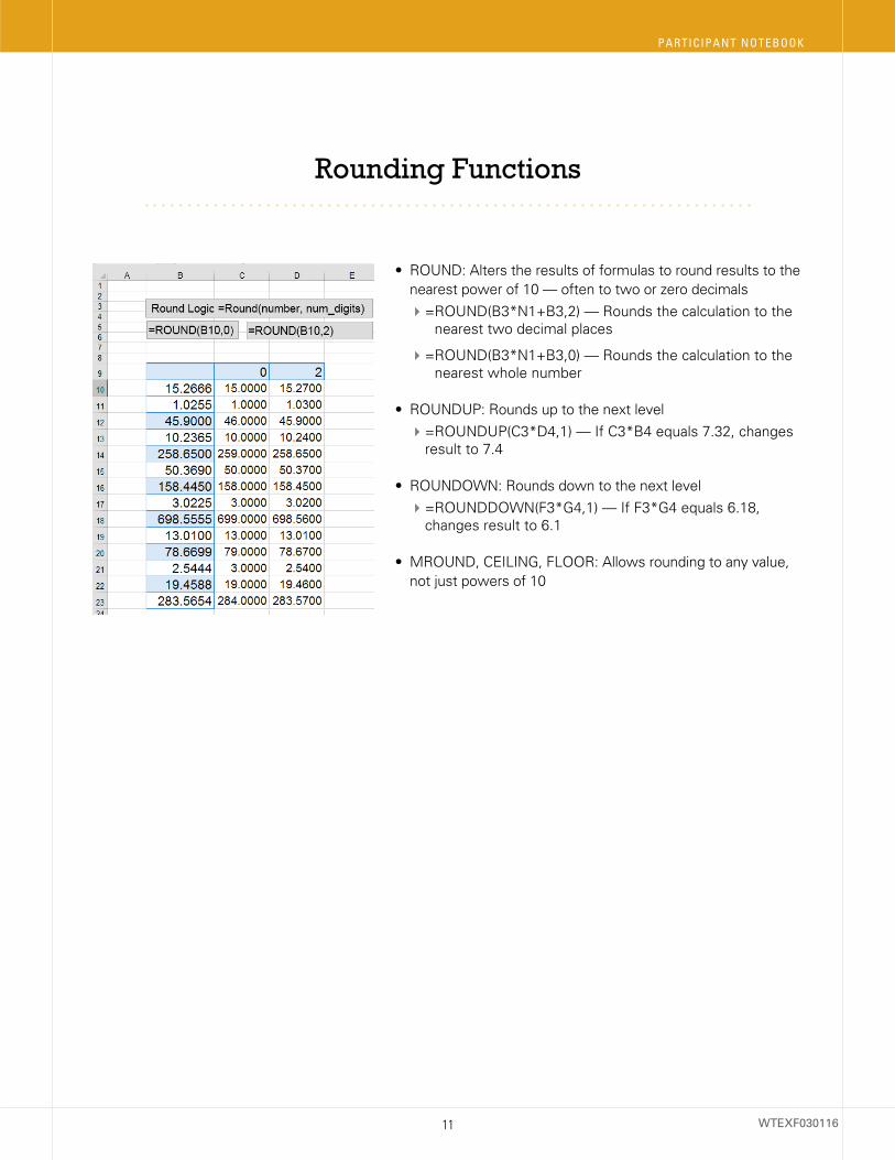
• ROUND: Alters the results of formulas to round results to the nearest power of 10 — often to two or zero decimals = ROUND(B3*N1+B3,2) — Rounds the calculation to the

nearest two decimal places

= ROUND(B3*N1+B3,0) — Rounds the calculation to the nearest whole number

• ROUNDUP: Rounds up to the next level =ROUNDUP(C3*D4,1) — If C3*B4 equals 7.32, changes

result to 7.4

• ROUNDOWN: Rounds down to the next level =ROUNDDOWN(F3*G4,1) — If F3*G4 equals 6.18,

changes result to 6.1

• MROUND, CEILING, FLOOR: Allows rounding to any value, not just powers of 10

Rounding Functions

11


WTEXF030116

1. TRIM: Eliminates leading and trailing spaces, as well as reducing multiple consecutive inner spaces to one space

• =TRIM(G3) — When G3 contains “North Dakota”, returns the text string “North Dakota”

2. PROPER: Returns text with the first letters of all words in uppercase, others in lowercase

3. UPPER: Returns text with all letters of all words in uppercase

4. LOWER: Returns text with all letters of all words in lowercase

5. Concatenation symbol (&): Puts together data from other cells and/or data strings

• =G3&”, “&H3 creates an entry consisting of the data from cell G3, then a comma and space, and then the data from H3.

Financial and Statistical Function OverviewFinancial Functions

• PMT: The loan payment function

• FV and RATE functions

Statistical Functions

• Popular functions: AVERAGE, MAX, MIN, MODE, MEDIAN

• Others: STDEV, VAR, PERCENTILE, QUARTILE, RANK, LARGE

Text Functions

12


WTEXF030116

Technical training only from our bookstore ...Training is our only business. That’s why our books and videos are uniquely focused on boosting your skills, expanding your capabilities and growing your career.

Our expert authors and presenters are professional trainers who don’t get bogged down in hype and fluff. They know how to zero in on the essentials, simplify complex subjects and not waste your time.

As a seminar participant, you always get the lowest price and fastest service because our resources are not sold through middlemen at discount stores, local booksellers or commercial Web sites.

B O O K S + S O F T W A R E + D V D S

Contact us: U.S./Canada 800-873-7545 • UK 0800 328 1140 • AUS 1800 145 231 • NZ 0800 447 301 Or visit us on the Web at www.ourbookstore.com

STAR12 is 365 DAYS of …

Peace of mind

Job help

Knowledge-packed seminars

Career development

Informative Webinars

Résumé boosters

Convenient on-line learning

Skill building

U N L I M I T E D T R A I N I N G Know that you have the resources and tools you need to achieve career success 365 days a year when you enroll in STAR12. With STAR12, you’ll get unlimited access to seminars, Webinars and on-line courses to help you do your job more effectively and efficiently. Put career success in your hands year round. Talk to your trainer to receive a special discount on STAR12, and enroll today!

VISIT JOINSTAR12.COM OR CALL 1-800-258-7246 FOR MORE INFORMATION

mastering excelimages.ruceci.com/pdfs/wtexfbook.pdf · · 2016-09-14mastering excel® functions...

Documents