matching models of the marriage market: theory and empirical
TRANSCRIPT

Matching models of the marriage market: theory andempirical applications
Pierre-André Chiappori Columbia University
Cemmap Masterclass, March 2011
P.A. Chiappori, Columbia () Matching modelsCemmap Masterclass, March 2011 1 /
20

Overview
Session 1: Background: Collective models of household behavior
Session 2: Matching models: theory (Part 1)
Session 3: Matching models: theory (Part 2)
Session 4: Matching models: applications
Session 5: Matching models: empirical applications (Part 1)
Session 6: Matching models: empirical applications (Part 2)
P.A. Chiappori, Columbia () Matching modelsCemmap Masterclass, March 2011 2 /
20

Overview
Session 1: Background: Collective models of household behavior
Session 2: Matching models: theory (Part 1)
Session 3: Matching models: theory (Part 2)
Session 4: Matching models: applications
Session 5: Matching models: empirical applications (Part 1)
Session 6: Matching models: empirical applications (Part 2)
P.A. Chiappori, Columbia () Matching modelsCemmap Masterclass, March 2011 3 /
20

Session 1
Background: Collective models of householdbehavior
P.A. Chiappori, Columbia () Matching modelsCemmap Masterclass, March 2011 4 /
20

Gains from marriage (what do we want to model?)
Ecclesiastes (4: 9-10) ; "Two are better than one, becausethey have a good reward for their toil. For if they fall, one willlift up the other; but woe to one who is alone and falls and doesnot have another to help. Again, if two lie together, they keepwarm; but how can one keep warm alone?"
P.A. Chiappori, Columbia () Matching modelsCemmap Masterclass, March 2011 5 /
20

Gains from marriage (what do we want to model?)
1 Sharing of public (non rival) goods. For instance, both partners canequally enjoy their children, share the same information and use thesame home.
2 Division of labor to exploit comparative advantage and increasingreturns to scale. For instance, one partner works at home and theother works in the market.
3 Home production. For example, coordinating child care, (which is apublic good for the parents).
4 Extending credit and coordination of investment activities. Forexample, one partner works when the other is in school.
5 Risk pooling. For example, one partner works when the other is sickor unemployed.
P.A. Chiappori, Columbia () Matching modelsCemmap Masterclass, March 2011 6 /
20

Modeling household behavior: the �unitary�framework
Drawbacks:
Contradicts individualism
Weak theoretical foundations
Samuelson: postulates a group utility W [U1, . . . ,US ]; W must beindependent of prices, wages, distribution factors,...Becker �rotten kid�: concludes that the group behaves as a singledecision maker.But: strong assumptions required:
Speci�c decision processTransferable utility and/or production functionIn a sense, assumes away most heterogeneity
Group as a �black box�
Group formation, dissolution,. . .Intragroup allocation ignored (inequality)�Power�issues ignored: income pooling (ex: targeting)
P.A. Chiappori, Columbia () Matching modelsCemmap Masterclass, March 2011 7 /
20

Modeling household behavior: the collective approach
Basic ideas:
Di¤erent individuals may have di¤erent preferences
Emphasis put on decision process
Hence: natural interpretation of �power�
Addresses issues of power redistribution: targeting, . . .
P.A. Chiappori, Columbia () Matching modelsCemmap Masterclass, March 2011 8 /
20

Modeling household behavior: the collective approach
General assumption: Pareto e¢ ciency
Justi�cations:
General principle (�no money left on the table�)Repeated interactionsCan be seen as a benchmark
Note, however, that commitment may be a problem
Basic insight:! powers summarized by Pareto weights
P.A. Chiappori, Columbia () Matching modelsCemmap Masterclass, March 2011 9 /
20

The collective approach: key concepts
Distribution factors:
Any factor that:- in�uences the decision process
- does not a¤ect preferences or budget sets
Examples: income, wealth ratios; control of land; background familyfactors; sex ratio; divorce laws; targeted bene�ts
Interpretation:
threat points in a bargaining contextsocial weight in a sociological interpretationstrategic position in a market contextetc.
P.A. Chiappori, Columbia () Matching modelsCemmap Masterclass, March 2011 10 /
20

The collective approach: main questions
Three main questions:
Testability (on demand data)
Identi�ability (recovering preferences and �power�); ! Distinctionidenti�ability/identi�cation
Theoretical underpinning: where do Pareto weights come from?
P.A. Chiappori, Columbia () Matching modelsCemmap Masterclass, March 2011 11 /
20

The collective approach: the setting
S agents; consumptions : public X 2 RN , private xs 2 Rn; note that(x1, ..., xS ) may not be observed.
Prices P, p; (group) income y ; intragroup production could beintroduced.
Distribution factors zk , k = 1, . . . ,K! could include individual incomes
Preferences : Us (X , x1, ..., xS ) (most general case)Particular cases:
�egoistic�: Us (X , xs )
�caring�: W shU1 (X , x1) , ...,US (X , xS )
iNote that: an allocation that is e¢ cient for caring is e¢ cient foregoistic as well
TU:Us (X , xs ) = F s
�As�X , x2s , ..., x
ns
�+ x1s b (X )
�P.A. Chiappori, Columbia () Matching models
Cemmap Masterclass, March 2011 12 /20

The collective approach: the setting
(Aggregate) market demand:
ξ = (X , x1 + ...+ xS )
as function of π = (P, p), y and possibly z ; budget constraint:
π0ξ = P 0X + p0 (x1 + ...+ xS ) = y
E¢ ciency: for all (p,P, y), there exist µ1, ..., µS withµ1 + ...+ µS = 1 such that (X , x1, . . . , xS ) solves:
maxX ,x1,...,xS
∑s
µsUs under the BC
or the more general version (with production):
maxX ,x1,...,xS
∑s
µsUs (P)
underΦ (X , x1 + ...+ xS ) = ξ and π0ξ = y
P.A. Chiappori, Columbia () Matching modelsCemmap Masterclass, March 2011 13 /
20

The collective approach: the setting
Key remark: in general, µ1, ..., µS depend on prices and incomes (anddistribution factors)
Therefore:
may de�ne household utility
UG (ξ, µ) = maxX ,x1,...,xS
∑s
µsUs s.t. Φ (X , x1 + ...+ xS ) = ξ
but it is price dependent.
Particular case: private goods only. Then e¢ ciency equivalent to theexistence of a sharing rule: there exists ρ = (ρ1, ..., ρS ) with∑ ρs = y such that xs solves
maxUs (xs ) st p0xs = ρs
Questions: testability and identi�cation
P.A. Chiappori, Columbia () Matching modelsCemmap Masterclass, March 2011 14 /
20

The collective approach: testability (price variations)
Normalization: y = 1; therefore Slutsky matrix S(π) = (Dπξ)�I � πξT
�Basic result (Browning-Chiappori 1998) :
Proposition
(The SNR(H � 1) condition). If the C 1 function ξ(π) solves problem(P), then the Slutsky matrix S(π) can be decomposed as:
S (π) = Σ (π) + R (π) (1)
where:
the matrix Σ (π) is symmetric and negativethe matrix R (π) is of rank at most H � 1.
Equivalently, there exists a subspace E (π) of dimension at least N + n� Ssuch that the restriction of S (π) to E (π) is symmetric, de�nite negative
P.A. Chiappori, Columbia () Matching modelsCemmap Masterclass, March 2011 15 /
20

The collective approach: testability (no price variation)
Engel curves: ξ i (y , z1, ..., zk )
De�nition of z-demands: assume there is at least one good j and oneobservable distribution factor, say z1, such that ξ j (y , z) strictlymonotone in z1. Then:
z1 = ζ(y , z�1, ξ j )
where z = (z1, z�1). Then substituting into the demand for good i 6= j :
ξ i (y , z1, z�1) = ξ i [y , ζ(y , z�1, ξ j ), z�1] = θij (y , z�1, ξj ).
P.A. Chiappori, Columbia () Matching modelsCemmap Masterclass, March 2011 16 /
20

The collective approach: testability (no price variation,BBC 2009)
PropositionA given system of demand functions is compatible with collectiverationality if and only if either K = 1 or it satis�es any of the following,equivalent conditions :i) there exist real valued functions Ξ1, .....,Ξn and µ such thatξ i (y , z) = Ξi [y , µ(y , z)] 8iii) household demand functions satisfy
∂ξ i/∂zk∂ξ i/∂zl
=∂ξ j/∂zk∂ξ j/∂zl
8i , j , k, l
iii) there exists at least one good j such that:
∂θij (y , z�1, ξj )
∂zk= 0 8i 6= j and k = 2, ..,K
P.A. Chiappori, Columbia () Matching modelsCemmap Masterclass, March 2011 17 /
20

The collective approach: identi�ability (C-E 2009)
Basic assumptions:
Egoistic preferences
Exclusion restrictions: for each agent s, there exists at elast onecommodity that s does not consume
Basic result (C-E 2009):
PropositionGenerically, the welfare relevant structure can be recovered
Moreover, in the absence of price variations, if all goods are private (orunder separability):
The sharing rule can be identi�ed up to a constant
Individual Engel curves can be recovered
Exclusion not needed!
P.A. Chiappori, Columbia () Matching modelsCemmap Masterclass, March 2011 18 /
20

The collective approach: empirical issues
Empirical tests:
various distribution factors (income, wealth ratios; control of land;background family factors; sex ratio; divorce laws; targeted bene�ts;...)various behavior: labor supply (CFL 2002), consumption ofgender-speci�c commodities (BBCL 1994), food consumption(Attanasio Lechene 2009), ...unitary restrictions generally rejected (income pooling)collective restrictions generally not rejected
Sex ratio: link with with the maket for marriage (Becker)
P.A. Chiappori, Columbia () Matching modelsCemmap Masterclass, March 2011 19 /
20

The collective approach: open issues
Dynamics and commitment
Risk and risk sharing
�Upstream�model: the collective model takes as given:
group compositiondecision process (Pareto weights)
! Questions:
group formation: who marries whom and why (and dissolution)?distribution of powers as an endogenous phenomenon
Basic tools:
bargaining theorymatching models (frictionless)search models (search frictions)
P.A. Chiappori, Columbia () Matching modelsCemmap Masterclass, March 2011 20 /
20

Matching models of the marriage market: theory andempirical applications
Pierre-André Chiappori Columbia University
Cemmap Masterclass, March 2011
P.A. Chiappori, Columbia () Matching modelsCemmap Masterclass, March 2011 1 /
43

Overview
Session 1: Background: Collective models of household behavior
Session 2: Matching models: theory (Part 1)
Session 3: Matching models: theory (Part 2)
Session 4: Matching models: applications
Session 5: Matching models: empirical applications (Part 1)
Session 6: Matching models: empirical applications (Part 2)
P.A. Chiappori, Columbia () Matching modelsCemmap Masterclass, March 2011 2 /
43

Session 2
Matching models: theory (1)
P.A. Chiappori, Columbia () Matching modelsCemmap Masterclass, March 2011 3 /
43

Background: The Collective Model
Takes as given:
group compositiondecision process (Pareto weights)
Questions:
group formation: who marries whom?distribution of powers as an endogenous phenomenon
Basic tools:
matching models (frictionless)search models (search frictions)bargaining theory
Here: emphasis on matching models; couples only; mostly TU
P.A. Chiappori, Columbia () Matching modelsCemmap Masterclass, March 2011 4 /
43

Transferable Utility (TU)
De�nitionA group satis�es TU if there exists monotone transformations of individualutilities such that the Pareto frontier is an hyperplane for all values ofprices and income.
In practice:
Quasi Linear (QL) preferences (but highly unrealistic)�Generalized Quasi Linear (GQL, Bergstrom and Cornes 1981):
us (qs ,Q) = Fs�As�q2s , ..., q
ns ,Q
�+ q1s bs (Q)
�with bs (Q) = b (Q) for all s
Note:
Ordinal propertyRestrictions on heterogeneityBut �acceptably�realistic
P.A. Chiappori, Columbia () Matching modelsCemmap Masterclass, March 2011 5 /
43

Properties of Transferable Utility (TU)
Unanimity regarding group�s decisions
clear distinction between aggregate behavior and intragroup allocationof power/resources/welfarehere: concentrate of �power�issues
Matching models: ! mathematical structure: optimal transportationmodels
P.A. Chiappori, Columbia () Matching modelsCemmap Masterclass, March 2011 6 /
43

Optimal Transportation Problems (Monge-Kantorovitch)
General Structure:
Complete, separable metric spaces X ,Y with measures F and GSurplus s (x , y) upper semicontinuousProblem: �nd a measure h on X � Y such that the marginals of h areF and G , and h solves
maxh
ZX�Y
s (x , y) dh (x , y)
Hence: linear programming
Dual problem: dual functions u (x) , v (y) and solve
minu,v
ZXu (x) dF (x) +
ZYv (y) dG (y)
under the constraint
u (x) + v (y) � s (x , y) for all (x , y) 2 X � Y
P.A. Chiappori, Columbia () Matching modelsCemmap Masterclass, March 2011 7 /
43

Optimal Transportation Problems (Monge-Kantorovitch)
General Structure:Complete, separable metric spaces X ,Y with measures F and G
Surplus s (x , y) upper semicontinuousProblem: �nd a measure h on X � Y such that the marginals of h areF and G , and h solves
maxh
ZX�Y
s (x , y) dh (x , y)
Hence: linear programming
Dual problem: dual functions u (x) , v (y) and solve
minu,v
ZXu (x) dF (x) +
ZYv (y) dG (y)
under the constraint
u (x) + v (y) � s (x , y) for all (x , y) 2 X � Y
P.A. Chiappori, Columbia () Matching modelsCemmap Masterclass, March 2011 7 /
43

Optimal Transportation Problems (Monge-Kantorovitch)
General Structure:Complete, separable metric spaces X ,Y with measures F and GSurplus s (x , y) upper semicontinuous
Problem: �nd a measure h on X � Y such that the marginals of h areF and G , and h solves
maxh
ZX�Y
s (x , y) dh (x , y)
Hence: linear programming
Dual problem: dual functions u (x) , v (y) and solve
minu,v
ZXu (x) dF (x) +
ZYv (y) dG (y)
under the constraint
u (x) + v (y) � s (x , y) for all (x , y) 2 X � Y
P.A. Chiappori, Columbia () Matching modelsCemmap Masterclass, March 2011 7 /
43

Optimal Transportation Problems (Monge-Kantorovitch)
General Structure:Complete, separable metric spaces X ,Y with measures F and GSurplus s (x , y) upper semicontinuousProblem: �nd a measure h on X � Y such that the marginals of h areF and G , and h solves
maxh
ZX�Y
s (x , y) dh (x , y)
Hence: linear programming
Dual problem: dual functions u (x) , v (y) and solve
minu,v
ZXu (x) dF (x) +
ZYv (y) dG (y)
under the constraint
u (x) + v (y) � s (x , y) for all (x , y) 2 X � Y
P.A. Chiappori, Columbia () Matching modelsCemmap Masterclass, March 2011 7 /
43

Matching Models under Transferable Utility
Becker-Shapley-Shubik (as opposed to Gale-Shapley)
Same general structure
Complete, separable metric spaces X ,Y with measures F and GSurplus s (x , y) upper semicontinuous
A matching consists of:
a measure h on X � Y such that the marginals of h are F and Gtwo functions u (x) , v (y) (�imputations�) such that
u (x) + v (y) = s (x , y) for all (x , y) 2 Supp (h)
Stability: the matching is stable if:
u (x) + v (y) � s (x , y) for all (x , y) 2 X � Y
Interpretation
P.A. Chiappori, Columbia () Matching modelsCemmap Masterclass, March 2011 8 /
43

Matching Models under Transferable Utility
Becker-Shapley-Shubik (as opposed to Gale-Shapley)
Same general structure
Complete, separable metric spaces X ,Y with measures F and GSurplus s (x , y) upper semicontinuous
A matching consists of:
a measure h on X � Y such that the marginals of h are F and Gtwo functions u (x) , v (y) (�imputations�) such that
u (x) + v (y) = s (x , y) for all (x , y) 2 Supp (h)
Stability: assume
u (x) + v (y) < s (x , y) for all (x , y) 2 X � Y
Interpretation
P.A. Chiappori, Columbia () Matching modelsCemmap Masterclass, March 2011 9 /
43

Matching Models under Transferable Utility
Becker-Shapley-Shubik (as opposed to Gale-Shapley)
Same general structure
Complete, separable metric spaces X ,Y with measures F and GSurplus s (x , y) upper semicontinuous
A matching consists of:
a measure h on X � Y such that the marginals of h are F and Gtwo functions u (x) , v (y) (�imputations�) such that
u (x) + v (y) = s (x , y) for all (x , y) 2 Supp (h)
Stability: the matching is stable if:
u (x) + v (y) � s (x , y) for all (x , y) 2 X � Y
Interpretation: �divorce at will�
P.A. Chiappori, Columbia () Matching modelsCemmap Masterclass, March 2011 10 /
43

Basic Result (duality)
We have the following:
TheoremA matching is stable if and only if it solves the surplus maximizationproblem
Consequence: existence; generic uniqueness of the measure underadditional conditions
Note that:
sets can be multidimensionalextends to hedonic models.
P.A. Chiappori, Columbia () Matching modelsCemmap Masterclass, March 2011 11 /
43

Basic Result (duality)
We have the following:
TheoremA matching is stable if and only if it solves the surplus maximizationproblem
Consequence: existence; generic uniqueness of the measure underadditional conditions
Note that:
sets can be multidimensional
extends to hedonic models.
P.A. Chiappori, Columbia () Matching modelsCemmap Masterclass, March 2011 11 /
43

Basic Result (duality)
We have the following:
TheoremA matching is stable if and only if it solves the surplus maximizationproblem
Consequence: existence; generic uniqueness of the measure underadditional conditions
Note that:
sets can be multidimensionalextends to hedonic models.
P.A. Chiappori, Columbia () Matching modelsCemmap Masterclass, March 2011 11 /
43

Hedonic Models
Structure:
Separable metric spaces X, Y, Z; measures F, GUtilities u(x,z) and c(z,y) upper semicontinuous;Problem: �nd a pricing function P(z) such that if:
x solves maxz u(x , z)� P(z)y solves maxz P (z)� c (y , z)
then markets clear
Basic property: equivalent to a matching with
s(x , y) = maxz(u(x , z)� c(y , z))
(see Chiappori-McCann-Neishem 2010)
Note that: n-dimensional; single crossing not needed; covexity notneeded.
P.A. Chiappori, Columbia () Matching modelsCemmap Masterclass, March 2011 12 /
43

Proof
Start from:
u(x) + v(y) � s (x , y) � u (x , z)� c (y , z) on X � Y � Z ,
hencec (y , z) + v (y) � u (x , z)� u(x) on X � Y � Z
andinfy2Y
fc (y , z) + v (y)g � supx2X
fu (x , z)� u (x)g on Z .
Take any P (z) such that
infy2Y
fc (y , z) + v (y)g � P (z) � supx2X
fu (x , z)� u (x)g on Z .
P.A. Chiappori, Columbia () Matching modelsCemmap Masterclass, March 2011 13 /
43

Supermodularity and assortative matching
One-dimensional:
s is supermodular if whenever x � x 0 and y � y 0 then
s (x , y) + s�x 0, y 0
�� s
�x , y 0
�+ s
�x 0, y
�Then stable matching is assortative; indeed, surplus maximization
Interpretation: single crossing (Spence - Mirrlees). Assume that s isC 1 then
s (x , y)� s�x 0, y
�� s
�x , y 0
�� s
�x 0, y 0
�and ∂s/∂x increasing in y ; if s is C 2 then
∂2s∂x∂y
� 0
Of course, similar results with submodularity (∂s/∂x decreasing in y)
In both case, ∂s/∂x monotonic in y ; if strict then injective
P.A. Chiappori, Columbia () Matching modelsCemmap Masterclass, March 2011 14 /
43

Supermodularity and assortative matching
Problem: both super- (or sub-) modularity and assortative matchingare typically one-dimensional
Generalization (CMcCN ET 2010):
De�nitionA surplus function s : X �Y �! [0,∞[ is said to be X�twisted if there isa set XL � X0 of zero volume such that ∂x s(x0, y1) is disjoint from∂x s(x0, y2) for all x0 2 X0 n XL and y1 6= y2 in Y .
Then the stable matching is unique and pure
De�nitionThe matching is pure if the measure µ is born by the graph of a function:for almost all x there exists exactly one y such that x matched with y .
! excludes �mixed strategies�
P.A. Chiappori, Columbia () Matching modelsCemmap Masterclass, March 2011 15 /
43

Counter example (C-McC-N 09)Transportation on a circle
P.A. Chiappori, Columbia () Matching modelsCemmap Masterclass, March 2011 16 /
43

Lake

Lake, students

Lake, students, schools

Counter example (C-McC-N 09)Transportation on a circle
Problem: allocate children to schoolsso as to minimize total transportation cost
Interpretation: matching with transfers (�tuition�)
Note that: single crossing cannot hold!
P.A. Chiappori, Columbia () Matching modelsCemmap Masterclass, March 2011 17 /
43

Counter example (C-McC-N 09)Transportation on a circle
Stable match:
P.A. Chiappori, Columbia () Matching modelsCemmap Masterclass, March 2011 18 /
43

Counter example (C-McC-N 09)Transportation on a circle
Stable match:
P.A. Chiappori, Columbia () Matching modelsCemmap Masterclass, March 2011 19 /
43

Application: marriage market
P.A. Chiappori, Columbia () Matching modelsCemmap Masterclass, March 2011 20 /
43

Application: marriage markets
Structure:
Men and women, respective income distributions F and G; mass 1 formen, r for womenTU; surplus s(x , y), derived from a collective modelIn general, TU implies s(x , y) supermodularExample (CIW07):
uh = Q�1+ qh
�uw = Q (a+ qw )
then
s (x , y) =(x + y + 1+ a)2
4Note that:
surplus depends on total income: s (x , y) = H (x + y)H convex (due to TU) therefore supermodularity
P.A. Chiappori, Columbia () Matching modelsCemmap Masterclass, March 2011 21 /
43

Application: marriage markets
Who marries whom? Assortative
Characterization: for any couple (x , y), the number of men withincome larger than x equals the number of women with income largerthan y :
1� F (x) = r (1� G (y))Therefore
x = φ (y) = F�1 [1� r (1� G (y))]
y = ψ (x) = G�1�1� 1
r(1� F (x))
�If r > 1 then y0 = ψ (0) �last married woman�
If r < 1 then x0 = φ (0) �last married man�
P.A. Chiappori, Columbia () Matching modelsCemmap Masterclass, March 2011 22 /
43

Matching with imperfectly transferable utility
General case: the Pareto frontier has the form
u = H (x , y , v) (1)
with H(0, 0, v) = 0 for all v . Here, H is decreasing in v and increasing inx and y .Two remarks:
stability can still be de�ned:
u (x) � H (x , y , v (y)) for all (x , y)
but no longer equivalent to surplus maximization
P.A. Chiappori, Columbia () Matching modelsCemmap Masterclass, March 2011 23 /
43

Session 3
Matching models: theory (2)
P.A. Chiappori, Columbia () Matching modelsCemmap Masterclass, March 2011 24 /
43

Sharing the surplus
Basic result:
Intramatch allocation of welfare is pinned downby the equilibrium conditions
P.A. Chiappori, Columbia () Matching modelsCemmap Masterclass, March 2011 25 /
43

Sharing the surplus
Stability impliesu (x) = max
y(s (x , y)� v (y))
therefore
u0 (x) =∂s∂x(x ,ψ (x)) and v 0 (y) =
∂s∂y(φ (y) , y)
and
u (x) = k +Z x
0
∂s∂x(t,ψ (t)) dt , v (y) = k 0 +
Z y
0
∂s∂y(φ (s) , s) ds
where k + k 0 given
Pinning down the constant: if r > 1 the �last married�womanreceives no surplus
Hence: endogeneize intrahousehold allocation
P.A. Chiappori, Columbia () Matching modelsCemmap Masterclass, March 2011 26 /
43

Sharing the surplus: application
Assume that s (x , y) = H (x + y), H convex. Then
u0 (x) = H 0 (x + ψ (x)) , v 0 (y) = H (φ (y) + y)
Application: �linear shift�: r = 1 and F (t) = G (αt � β) for someα < 1, β > 0
Satis�ed for instance if Lognormal distributions with same σ.P.A. Chiappori, Columbia () Matching models
Cemmap Masterclass, March 2011 27 /43

Example: shifting female income distribution
Then φ (y) = (y + β) /α and ψ (x) = αx � β; from
u0 (x) = H 0 ((α+ 1) x � β) ,
one gets
u (x) = K 0 +1
1+ αH (x + ψ (x))
and
v (y) = K +α
1+ αH (φ (y) + y)
where K +K 0 = 0
P.A. Chiappori, Columbia () Matching modelsCemmap Masterclass, March 2011 28 /
43
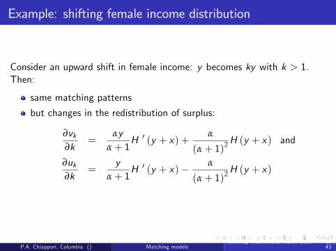
Example: shifting female income distribution
Consider an upward shift in female income: y becomes ky with k > 1.Then:
same matching patterns
but changes in the redistribution of surplus:
∂vk∂k
=αy
α+ 1H 0 (y + x) +
α
(α+ 1)2H (y + x) and
∂uk∂k
=y
α+ 1H 0 (y + x)� α
(α+ 1)2H (y + x)
P.A. Chiappori, Columbia () Matching modelsCemmap Masterclass, March 2011 29 /
43

Example: shifting female income distribution
Consider an upward shift in female income: y becomes ky with k > 1.Then:
same matching patterns
but changes in the redistribution of surplus:
∂vk∂k
=αy
α+ 1H 0 (y + x)
∂uk∂k
=y
α+ 1H 0 (y + x)
P.A. Chiappori, Columbia () Matching modelsCemmap Masterclass, March 2011 30 /
43

Example: shifting female income distribution
Consider an upward shift in female income: y becomes ky with k > 1.Then:
same matching patterns
but changes in the redistribution of surplus:
∂vk∂k
=αy
α+ 1H 0 (y + x) +
α
(α+ 1)2H (y + x) and
∂uk∂k
=y
α+ 1H 0 (y + x)� α
(α+ 1)2H (y + x)
P.A. Chiappori, Columbia () Matching modelsCemmap Masterclass, March 2011 31 /
43

Matching with imperfectly transferable utility
As above, stability implies that:
u (x) = maxyH(x , y , v (y))
where the maximum is actually reached for y = ψ (x) (or x = φ (y)).First order conditions imply that
∂H∂y(φ (y) , y , v (y)) + v 0 (y)
∂H∂v(φ (y) , y , v (y)) = 0.
or:
v 0 (y) = �∂H∂y (φ (y) , y , v (y))∂H∂v (φ (y) , y , v (y))
.
and
u0 (x) =∂H∂x(x ,ψ (x) , v (ψ (x)))
P.A. Chiappori, Columbia () Matching modelsCemmap Masterclass, March 2011 32 /
43

Matching with imperfectly transferable utility
Second order conditions:
∂
∂y
�∂H∂y(φ (y) , y , v (y)) + v 0 (y)
∂H∂v(φ (y) , y , v (y))
�� 0 8y .
Since
F (y , φ (y)) = 0 8ywhere
F (y , x) =∂H∂y(x , y , v (y)) + v 0 (y)
∂H∂v(x , y , v (y)) .
we have:∂F∂y+
∂F∂x
φ0 (y) = 0 8y ,
which implies that
∂F∂y� 0 if and only if
∂F∂x
φ0 (y) � 0.
P.A. Chiappori, Columbia () Matching modelsCemmap Masterclass, March 2011 33 /
43

Matching with imperfectly transferable utility
The second order conditions can hence be written as:�∂2H∂x∂y
(φ (y) , y , v (y)) + v 0 (y)∂2H∂x∂v
(φ (y) , y , v (y))�
φ0 (y) � 0 8y .(2)
Assortative matching: φ0 (y) � 0, which holds if
∂2H∂x∂y
(φ (y) , y , v (y)) + v 0 (y)∂2H∂x∂v
(φ (y) , y , v (y)) � 0 8y . (3)
Since v 0 (y) � 0, a su¢ cient (although obviously not necessary) conditionis that
∂2H∂x∂y
(φ (y) , y , v (y)) � 0 and ∂2H∂x∂v
(φ (y) , y , v (y)) � 0. (4)
Note: under TU, H (x , y , v (y)) = h (x , y)� v (y) and ∂2H∂x∂v = 0
P.A. Chiappori, Columbia () Matching modelsCemmap Masterclass, March 2011 34 /
43

Matching with imperfectly transferable utility
v
u
P
P’
Figure: The slope conditionP.A. Chiappori, Columbia () Matching models
Cemmap Masterclass, March 2011 35 /43

Matching with imperfectly transferable utility: an example
continuum of males (income x distributed over [a,A], cdf F )
continuum of females (income y distributed over [b,B ] cdf G ).
Linear shift case φ (y) = (y + β) /α and ψ (x) = αx � β
Number of female is almost equal to, but slightly larger than that ofmen
Male preferences: Cobb-Douglas
um = cmQ
Female preferences: perfect substitutes
uf (cf ) = �∞ if cf < c
= cf +Q if cf � c
In particular, if a woman is single, her income must be at least c ; thenher utility equals her income.
P.A. Chiappori, Columbia () Matching modelsCemmap Masterclass, March 2011 36 /
43

Matching with imperfectly transferable utility: an example
E¢ cient allocations:max cmQ
under the constraints
cm + cf +Q = x + y , uf = cf +Q � U
Remark: at any e¢ cient allocation:
cf = cU � ((x + y) + c) /2.
Pareto frontier:
um = H ((x + y) , uf ) = (uf � c) ((x + y)� uf ) , (5)
where uf � (x+y )+c2 ,and Q = uf � c , cm = (x + y)� uf .
P.A. Chiappori, Columbia () Matching modelsCemmap Masterclass, March 2011 37 /
43

3.0 3.2 3.4 3.6 3.8 4.0 4.2 4.4 4.6 4.8 5.0 5.20
1
2
3
4
u
v
Figure: Pareto frontier
P.A. Chiappori, Columbia () Matching modelsCemmap Masterclass, March 2011 38 /
43

Characterization
∂H (x + y , v)∂ (x + y)
= v � c , ∂H (x + y , v)∂v
= � (2v � (c + (x + y)))
therefore assortative matching since
∂2H (x + y , v)
∂ (x + y)2= 0 and
∂2H (x + y , v)∂ (x + y) ∂v
= 1
Moreover:
v 0 (y) =αv (y)� αc
2αv (y)� (α+ 1) y � (αc + β)> 0 (6)
P.A. Chiappori, Columbia () Matching modelsCemmap Masterclass, March 2011 39 /
43

2.0 2.2 2.4 2.6 2.8 3.0 3.2 3.4 3.6 3.8 4.0 4.2 4.4
2
4
6
8
x
Utilities
Figure: Husband�s and Wife�s Utilities, Public Consumption and the Husband�sPrivate Consumption (β = 0, α = .8)
P.A. Chiappori, Columbia () Matching modelsCemmap Masterclass, March 2011 40 /
43

Summary
matching as tractable way of modeling general equilibrium interactions
main advantage: explicit derivation of the sharing rule
TU: equivalent to linear programming
More general models are feasible
P.A. Chiappori, Columbia () Matching modelsCemmap Masterclass, March 2011 41 /
43

P.A. Chiappori, Columbia () Matching modelsCemmap Masterclass, March 2011 42 /
43

P.A. Chiappori, Columbia () Matching modelsCemmap Masterclass, March 2011 43 /
43

Matching models of the marriage market: theory andempirical applications
Pierre-André Chiappori Columbia University
Cemmap Masterclass, March 2011
P.A. Chiappori, Columbia () Matching modelsCemmap Masterclass, March 2011 1 /
18

Overview
Session 1: Background: Collective models of household behavior
Session 2: Matching models: theory (Part 1)
Session 3: Matching models: theory (Part 2)
Session 4: Matching models: applications
Session 5: Matching models: empirical applications (Part 1)
Session 6: Matching models: empirical applications (Part 2)
P.A. Chiappori, Columbia () Matching modelsCemmap Masterclass, March 2011 2 /
18

Session 4
Matching models: Applications
P.A. Chiappori, Columbia () Matching modelsCemmap Masterclass, March 2011 3 /
18

Applications: applied theory
Various applications:
Calibration: impact of female education on intrahousehold allocation
Abortion and female empowerment (CO JPE 2006)
Children and divorce (CW JoLE 2007)
Male and female demand for higher education (CIW AER 2009)
Dynamics: divorce and impact of divorce laws (CIW 10)
P.A. Chiappori, Columbia () Matching modelsCemmap Masterclass, March 2011 4 /
18

Motivation: education and marriage, US
P.A. Chiappori, Columbia () Matching modelsCemmap Masterclass, March 2011 5 /
18

Motivation: education and marriage, USEducation
P.A. Chiappori, Columbia () Matching modelsCemmap Masterclass, March 2011 6 /
18

Motivation: education and marriage, USEducation
P.A. Chiappori, Columbia () Matching modelsCemmap Masterclass, March 2011 7 /
18

Asymmetric reactions to increasing returns to education
Possible explanations:
1 Gender discrimination smaller for high incomes?2 Ability?3 Intrahousehold e¤ects
Returns to education have two components: market and intrahouseholdIf larger percentage of educated women, a¤ects matching patternsCost of not being educated are higher
P.A. Chiappori, Columbia () Matching modelsCemmap Masterclass, March 2011 8 /
18

P.A. Chiappori, Columbia () Matching modelsCemmap Masterclass, March 2011 9 /
18

P.A. Chiappori, Columbia () Matching modelsCemmap Masterclass, March 2011 10 /
18

The model
Two equally large populations of men and women to be matched.
Individuals live two periods; investment takes place in the �rst periodof life and marriage in the second period; investment in schooling islumpy and takes one period.
All agents of the same level of schooling and gender receive the samewage.
I (i) and J(j) are the schooling "class" of man i and woman j (1 ifuneducated, 2 if educated)
Transferable utility; marital surplus if man i marries woman j:
sij = zI (i )J (j) + θi + θj
withz11 + z22 > z12 + z21
P.A. Chiappori, Columbia () Matching modelsCemmap Masterclass, March 2011 11 /
18

The model
Investment in schooling is associated with idiosyncratic cost (bene�t),µi for men and µj for women.
θ and µ independent from each other and independent acrossindividuals; distributions F (θ) and G (µ).
Shadow price of woman j is uj , shadow price of man i is vi ; stability:
zI (i )J (j) + θi + θj � vi + uj
therefore
vi = max�maxj
�zI (i )J (j) + θi + θj � uj
�, 0�
uj = max�maxi
�zI (i )J (j) + θi + θj � vi
�, 0�
P.A. Chiappori, Columbia () Matching modelsCemmap Masterclass, March 2011 12 /
18

θ1V−2V−
b
mR
2 1mR V V+ −
µ
Investment,no marriage
Marriage, noinvestment
Marriage andinvestment
No marriage,no investment
P.A. Chiappori, Columbia () Matching modelsCemmap Masterclass, March 2011 13 /
18

The model
Proposition:
vi = VI (i ) + θi
uj = UJ (j) + θj
with
VI = maxJ(zIJ � UJ )
UJ = maxI(zIJ � VI )
P.A. Chiappori, Columbia () Matching modelsCemmap Masterclass, March 2011 14 /
18

The model
Theorem:
U1 + V1 = z11U2 + V2 = z22
and either strict assortative matching:
U1 + V2 � z21U2 + V1 � z12
or some people �marry down�. If more educated men:
U1 + V2 = z21 therefore U2 � U1 = z22 � z21,V2 � V1 = z21 � z11
whereas if more educated women:
U2 + V1 = z12 therefore U2 � U1 = z12 � z11,V2 � V1 = z22 � z21
P.A. Chiappori, Columbia () Matching modelsCemmap Masterclass, March 2011 15 /
18

The model
Equilibrium equations:
Example: # married men = # married women
F (V1)+
V2ZV1
G (Rm +V2� θ)f (θ)dθ = F (U1)+
U2ZU1
G (Rw +U2� θ)f (θ)dθ,
Example: # educated married men = # educated married women
F (V1) [1� G (Rm + V2 � V1)] = F (U1) [1� G (Rw + U2 � U1)]
Then calibration
P.A. Chiappori, Columbia () Matching modelsCemmap Masterclass, March 2011 16 /
18

Comparative statics
Compare an "old" regime a "new" regime.
In the old regime:lower returns to educationmore time to be spent at home ! specialization
New regime:higher returns to educationless time spent at home ! both genders demand education
Initial sources of asymmetry?statistical discrimination weaker against educated womendi¤erences in innate ability (Becker-Hubbard-Murphy)impact of birth control
Equilibrium mechanism ampli�es the shiftOld regime: some men marry down, marital returns of schooling higherfor menNew regime: just the opposite (�you can�t a¤ord to be a nurse�)
P.A. Chiappori, Columbia () Matching modelsCemmap Masterclass, March 2011 17 /
18

P.A. Chiappori, Columbia () Matching modelsCemmap Masterclass, March 2011 18 /
18

Matching models of the marriage market: theory andempirical applications
Pierre-André Chiappori, Columbia University
Cemmap Masterclass, March 2011
P.A. Chiappori, Columbia () Matching modelsCemmap Masterclass, March 2011 1 /
34

Overview
Session 1: Background: Collective models of household behavior
Session 2: Matching models: theory (Part 1)
Session 3: Matching models: theory (Part 2)
Session 4: Matching models: applications
Session 5: Matching models: empirical applications (Part 1)
Session 6: Matching models: empirical applications (Part 2)
P.A. Chiappori, Columbia () Matching modelsCemmap Masterclass, March 2011 2 /
34

Session 5
Matching models: empirical applications
Part 1: a semi-structural model
P.A. Chiappori, Columbia () Matching modelsCemmap Masterclass, March 2011 3 /
34

Motivation: education and marriage, US
P.A. Chiappori, Columbia () Matching modelsCemmap Masterclass, March 2011 4 /
34

Motivation: education and marriage, USEducation
P.A. Chiappori, Columbia () Matching modelsCemmap Masterclass, March 2011 5 /
34

Motivation: education and marriage, USEducation
P.A. Chiappori, Columbia () Matching modelsCemmap Masterclass, March 2011 6 /
34

Motivation: education and marriage, USMarital patterns
P.A. Chiappori, Columbia () Matching modelsCemmap Masterclass, March 2011 7 /
34

Motivation: education and marriage, USMarital patterns
P.A. Chiappori, Columbia () Matching modelsCemmap Masterclass, March 2011 8 /
34

Motivation: education and marriage, USMarital patterns
P.A. Chiappori, Columbia () Matching modelsCemmap Masterclass, March 2011 9 /
34

Motivation: education and marriage, USMarital patterns
Burtless (EER 1999): over 1979-1996:�The changing correlation of husband and wife earnings has tended toreinforce the e¤ect of greater pay disparity.�
Maybe 1/3 of the increase in household-level inequality (Gini) comesfrom rise of single-adult households and 1/6 from increasedassortative matching. Burtless again, US 1979-1996:�The Spearman rank correlation of husband and wife earningsincreased from .012 to .145�
P.A. Chiappori, Columbia () Matching modelsCemmap Masterclass, March 2011 10 /
34

Questions
1 Education: Why the asymmetric response between men and women?Possible answer (CIW, AER 2009): �Marital College Premium�! Is there evidence for a MCP?
2 Changes in matching patterns:
change in attitudes toward assortative matching?or only a mechanical consequences of the changes in populationcompositions?
3 Matching models: scope and empirical implementation
Basic tool: frictionless matching
Reference:
Choo and Siow (JPE 2003)Chiappori, Salanié and Weiss 2010
P.A. Chiappori, Columbia () Matching modelsCemmap Masterclass, March 2011 11 /
34

Questions
1 Education: Why the asymmetric response between men and women?Possible answer (CIW, AER 2009): �Marital College Premium�! Is there evidence for a MCP?
2 Changes in matching patterns:
change in attitudes toward assortative matching?
or only a mechanical consequences of the changes in populationcompositions?
3 Matching models: scope and empirical implementation
Basic tool: frictionless matching
Reference:
Choo and Siow (JPE 2003)Chiappori, Salanié and Weiss 2010
P.A. Chiappori, Columbia () Matching modelsCemmap Masterclass, March 2011 11 /
34

Questions
1 Education: Why the asymmetric response between men and women?Possible answer (CIW, AER 2009): �Marital College Premium�! Is there evidence for a MCP?
2 Changes in matching patterns:
change in attitudes toward assortative matching?or only a mechanical consequences of the changes in populationcompositions?
3 Matching models: scope and empirical implementation
Basic tool: frictionless matching
Reference:
Choo and Siow (JPE 2003)Chiappori, Salanié and Weiss 2010
P.A. Chiappori, Columbia () Matching modelsCemmap Masterclass, March 2011 11 /
34

Questions
1 Education: Why the asymmetric response between men and women?Possible answer (CIW, AER 2009): �Marital College Premium�! Is there evidence for a MCP?
2 Changes in matching patterns:
change in attitudes toward assortative matching?or only a mechanical consequences of the changes in populationcompositions?
3 Matching models: scope and empirical implementation
Basic tool: frictionless matching
Reference:
Choo and Siow (JPE 2003)
Chiappori, Salanié and Weiss 2010
P.A. Chiappori, Columbia () Matching modelsCemmap Masterclass, March 2011 11 /
34

Questions
1 Education: Why the asymmetric response between men and women?Possible answer (CIW, AER 2009): �Marital College Premium�! Is there evidence for a MCP?
2 Changes in matching patterns:
change in attitudes toward assortative matching?or only a mechanical consequences of the changes in populationcompositions?
3 Matching models: scope and empirical implementation
Basic tool: frictionless matching
Reference:
Choo and Siow (JPE 2003)Chiappori, Salanié and Weiss 2010
P.A. Chiappori, Columbia () Matching modelsCemmap Masterclass, March 2011 11 /
34

Empirical implementation
Basic issue: capturing imperfections (frictions) in the matching process
Various strategies:
Random matching (Shimer-Smith)
Search
Frictionless matching with unobservable components
P.A. Chiappori, Columbia () Matching modelsCemmap Masterclass, March 2011 12 /
34

Empirical implementation
Basic insight: unobserved characteristics (heterogeneity)! Gain g IJij generated by the match i 2 I , j 2 J:
g IJij = ZIJ + εIJij
where I = 0, J = 0 for singles, and εIJij random shock with mean zero.
Therefore: dual variables (ui , vj ) also random (endogenousdistribution)
Stability: constrained by the inequalities
ui + vj � g IJij for any (i , j)
! large number (one inequality per potential couple)
P.A. Chiappori, Columbia () Matching modelsCemmap Masterclass, March 2011 13 /
34

Empirical implementation
Crucial identifying assumption (Choo-Siow 2006)Assumption S (separability): the idiosyncratic component εij isadditively separable:
εIJij = αIJi + βIJj (S)
where E�αIJi�= E
hβIJj
i= 0.
Then:
Theorem
Under S, there exists U IJ and V IJ such that U IJ + V IJ = Z IJ and for anymatch (i 2 I , j 2 J)
ui = U IJ + αIJi
vj = V IJ + βIJj
General characterization: Galichon-Salanie (2011)
P.A. Chiappori, Columbia () Matching modelsCemmap Masterclass, March 2011 14 /
34

Galichon-Salanié 2011
Assume separability, let πIJ the proba that i 2 I marries j 2 J; thenSocial surplus is
Σ = 2∑i ,j
πIJZIJ + ε (nI , nJ ,π)
where ε is a �generalized entropy�
When α, β are extreme values, then
ε (nI , nJ ,π) = �∑I
∑J
πIJ lnπIJnI�∑
I∑J
πIJ lnπIJnJ,
Can be used for identi�cation
P.A. Chiappori, Columbia () Matching modelsCemmap Masterclass, March 2011 15 /
34

Empirical implementation
TheoremA NSC for i 2 I being matched with a spouse in J is:
U IJ + αIJi � U I0 + αI0i
U IJ + αIJi � U IK + αIKi for all K
In practice:
take singlehood as a benchmark (interpretation!)assume the αIJi are extreme value distributedthen logit and expected utility:
uI = E�maxJ
�U IJ + αIJi
��= ln
∑JexpU IJ + 1
!= � ln
�aI0�
Problem: can we compare the u across classes?
needed (marital college premium)but relies on a strong assumption (�What is the unit?�)
P.A. Chiappori, Columbia () Matching modelsCemmap Masterclass, March 2011 16 /
34

Empirical implementation
TheoremA NSC for i 2 I being matched with a spouse in J is:
U IJ + αIJi � U I0 + αI0i
U IJ + αIJi � U IK + αIKi for all K
In practice:take singlehood as a benchmark (interpretation!)
assume the αIJi are extreme value distributedthen logit and expected utility:
uI = E�maxJ
�U IJ + αIJi
��= ln
∑JexpU IJ + 1
!= � ln
�aI0�
Problem: can we compare the u across classes?
needed (marital college premium)but relies on a strong assumption (�What is the unit?�)
P.A. Chiappori, Columbia () Matching modelsCemmap Masterclass, March 2011 16 /
34

Empirical implementation
TheoremA NSC for i 2 I being matched with a spouse in J is:
U IJ + αIJi � U I0 + αI0i
U IJ + αIJi � U IK + αIKi for all K
In practice:take singlehood as a benchmark (interpretation!)assume the αIJi are extreme value distributed
then logit and expected utility:
uI = E�maxJ
�U IJ + αIJi
��= ln
∑JexpU IJ + 1
!= � ln
�aI0�
Problem: can we compare the u across classes?
needed (marital college premium)but relies on a strong assumption (�What is the unit?�)
P.A. Chiappori, Columbia () Matching modelsCemmap Masterclass, March 2011 16 /
34

Empirical implementation
TheoremA NSC for i 2 I being matched with a spouse in J is:
U IJ + αIJi � U I0 + αI0i
U IJ + αIJi � U IK + αIKi for all K
In practice:take singlehood as a benchmark (interpretation!)assume the αIJi are extreme value distributedthen logit and expected utility:
uI = E�maxJ
�U IJ + αIJi
��= ln
∑JexpU IJ + 1
!= � ln
�aI0�
Problem: can we compare the u across classes?
needed (marital college premium)but relies on a strong assumption (�What is the unit?�)
P.A. Chiappori, Columbia () Matching modelsCemmap Masterclass, March 2011 16 /
34

Empirical implementation
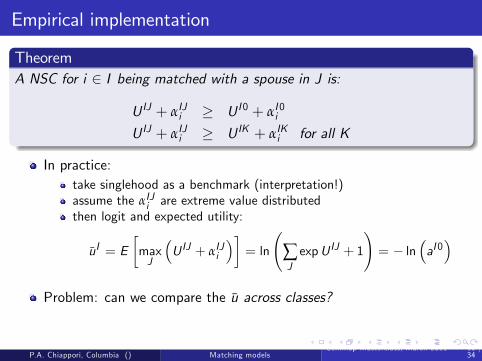
TheoremA NSC for i 2 I being matched with a spouse in J is:
U IJ + αIJi � U I0 + αI0i
U IJ + αIJi � U IK + αIKi for all K
In practice:take singlehood as a benchmark (interpretation!)assume the αIJi are extreme value distributedthen logit and expected utility:
uI = E�maxJ
�U IJ + αIJi
��= ln
∑JexpU IJ + 1
!= � ln
�aI0�
Problem: can we compare the u across classes?needed (marital college premium)
but relies on a strong assumption (�What is the unit?�)
P.A. Chiappori, Columbia () Matching modelsCemmap Masterclass, March 2011 16 /
34

Empirical implementation
TheoremA NSC for i 2 I being matched with a spouse in J is:
U IJ + αIJi � U I0 + αI0i
U IJ + αIJi � U IK + αIKi for all K
In practice:take singlehood as a benchmark (interpretation!)assume the αIJi are extreme value distributedthen logit and expected utility:
uI = E�maxJ
�U IJ + αIJi
��= ln
∑JexpU IJ + 1
!= � ln
�aI0�
Problem: can we compare the u across classes?needed (marital college premium)but relies on a strong assumption (�What is the unit?�)
P.A. Chiappori, Columbia () Matching modelsCemmap Masterclass, March 2011 16 /
34

Empirical implementation
Extension: heteroskedasticity
εIJij = σiαIJi + µjβ
IJj (1)
then
ui = U IJ + σI αIJi
vj = V IJ + µJ βIJj
and conditions become:
U IJ
σI+ αIJi � U I0
σI+ αI0i
U IJ
σI+ αIJi � U IK
σI+ αIKi for all K
P.A. Chiappori, Columbia () Matching modelsCemmap Masterclass, March 2011 17 /
34

Why does heteroskedasticity matter?
Homoskedastic version: marital college premium measured by thedi¤erence uI � uK (I = college, K = high school) and
uI � uK = ln�aK 0
aI0
�Intuition:
people marry if their (idiosyncratic) gain is larger than some threshold.homoskedastic: one-to-one mapping between the mean and thepercentage below the threshold
P.A. Chiappori, Columbia () Matching modelsCemmap Masterclass, March 2011 18 /
34

Why does heteroskedasticity matter?
Heteroskedastic version: now
uI � uK = σK ln�aK 0�� σI ln
�aI0�
and the one-to-one mapping is lost!
P.A. Chiappori, Columbia () Matching modelsCemmap Masterclass, March 2011 19 /
34

Covariates
αIJi = Xi .ζIJm + αIJi
βIJj = Yj .ζIJf + β
IJj
and
aIJ = Pr (i , characteristics Xi , matched with a female in J)
=exp
�U IJ + Xi .ζ
IJm
�∑K exp
�U IK + Xi .ζ
IKm
�+ exp
�U I0 + Xi .ζ
I0m
�!standard logit
P.A. Chiappori, Columbia () Matching modelsCemmap Masterclass, March 2011 20 /
34

Test and identi�cation: cross sectional data
Basic result:
homoskedastic model exactly identi�ed
heteroskedastic model not identi�ed
Argument (Choo-Siow 2006):
aIJ = Pr (i matched with a female in J)
=exp
�U IJ/σI
�∑K exp (U IK/σI ) + 1
therefore one-to-one correspondence between the aIJ (observed) and theU IJ/σI .
P.A. Chiappori, Columbia () Matching modelsCemmap Masterclass, March 2011 21 /
34

Test and identi�cation: dynamic data
Idea: structural modelM =�Z IJ , σI , µJ
�holds for di¤erent cohorts
c = 1, ...,T with varying class compositions. Then:
gij ,c = Z IJc + σI αIJi ,c + µJ βIJj ,c
with the identifying assumption:
Z IJc = ζ Ic + ξJc + ZIJ
Interpretation: trend a¤ecting the surplus but not the supermodularity
Z IJc � Z ILc � ZKJc + ZKLc = Z IJ � Z IL � ZKJ + ZKL
Normalizations
ζ I1 = ξJ1 = 0 so that ZIJ = Z IJ1 .
For any c > 1, the ζ Ic and ξJc are only de�ned up to a (common)additive constant, therefore ξ1c = 0 for all c .
P.A. Chiappori, Columbia () Matching modelsCemmap Masterclass, March 2011 22 /
34

Test and identi�cation: dynamic dataTest
Start from:
aIJc = Pr (i 2 I matched with a female in J at c) =exp
�U IJc /σI
�1+∑K exp (UKJc /σK )
De�ne pIJc = UIJc /σI , qIJc = V
IJc /µJ , then
pIJc = ln�
aIJc1�∑K aIKc
�and σI pIJc + µJ qIJc = ζ Ic + ξJc + Z
IJ
gives for all (I � 2, J � 2):
p1Jc � p11c = σI�pIJc � pI1c
�+ µJ
�qIJc � q1Jc
�� µ1
�qI1c � q11c
���Z IJ � Z I1 � Z 1J + Z 11
�P.A. Chiappori, Columbia () Matching models
Cemmap Masterclass, March 2011 23 /34

Test and identi�cation: dynamic dataTest
De�ne the vectors:
PIJ =�pIJ1 � pI11 , ..., pIJT � pI1T
�QIJ =
�qIJ1 � q1J1 , ..., qIJT � q1JT
�RIJ =
�p1J1 � p111 , ..., p1JT � p11T
�1 = (1, ..., 1)
Then for each pair (I � 2, J � 2):
RIJ = σI PIJ + µJ QIJ � µ1QI1 ��Z IJ � Z I1 � Z 1J + Z 11
�1
therefore:
RIJ belongs to the subspace generated by�PIJ ,QIJ ,QI1, 1
,
the coe¢ cient of PIJ (resp. QIJ ,resp. QI1) does not depend on J(resp. I , resp. is constant).
P.A. Chiappori, Columbia () Matching modelsCemmap Masterclass, March 2011 24 /
34

Test and identi�cation: dynamic dataIdenti�cation
From
RIJ = σI PIJ + µJ QIJ � µ1QI1 ��Z IJ � Z I1 � Z 1J + Z 11
�1
we (over)identify σI , µJ and�Z IJ � Z I1 � Z 1J + Z 11
�For c = 1:
σI pIJ1 + µJ qIJ1 = ZIJ
identi�es Z IJ
ThenσI pI1c + µ1 qI1c = ζ Ic + Z
I1 8I , 1, cidenti�es ζ Ic , and ξJc follows
In practice: minimum distance.
P.A. Chiappori, Columbia () Matching modelsCemmap Masterclass, March 2011 25 /
34

Data
American Community Survey, a representative extract of Census. The2008 survey has info on current marriage status, number of marriages,year of current marriage (633,885 currently married couples).
Born between 1943 and 1970 for men, 1945 and 1972
Three education classes: HS drop out, HS graduate, College andabove
Construct 28 �cohorts�; for each cohort, matrix of marriageproportions by classes (plus singles)
Age ! assumption: husband in cohort c marries wife in cohort c + 2
P.A. Chiappori, Columbia () Matching modelsCemmap Masterclass, March 2011 26 /
34
Results (1)
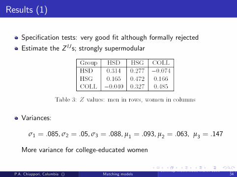
Speci�cation tests: very good �t although formally rejected
Estimate the Z IJ s; strongly supermodular
Variances:
σ1 = .085, σ2 = .05, σ3 = .088, µ1 = .093, µ2 = .063, µ3 = .147
More variance for college-educated women
P.A. Chiappori, Columbia () Matching modelsCemmap Masterclass, March 2011 27 /
34

Results: trends
Surplus of diagonal matches
P.A. Chiappori, Columbia () Matching modelsCemmap Masterclass, March 2011 28 /
34

Results: marital college premium
In principle, marital college premium has several components:
Marriage probabilitySpouse�s (distribution of) educationSurplus generatedDistribution of the surplus
Our estimates for women:
Year born 1945-47 1970-72Marriage Probability HS 94% Coll 89% HS 78% Coll 81%Coll Educated Spouse HS 39% Coll 84% HS 38% Coll 84%Surplus (Coll Husband) HS .258 Coll .473 HS -.10 Coll .286Share (Coll Husband) HS 47% Coll 51% HS 45% Coll 57%
P.A. Chiappori, Columbia () Matching modelsCemmap Masterclass, March 2011 29 /
34

Results: marital college premium
In principle, marital college premium has several components:
Marriage probability
Spouse�s (distribution of) educationSurplus generatedDistribution of the surplus
Our estimates for women:
Year born 1945-47 1970-72Marriage Probability HS 94% Coll 89% HS 78% Coll 81%Coll Educated Spouse HS 39% Coll 84% HS 38% Coll 84%Surplus (Coll Husband) HS .258 Coll .473 HS -.10 Coll .286Share (Coll Husband) HS 47% Coll 51% HS 45% Coll 57%
P.A. Chiappori, Columbia () Matching modelsCemmap Masterclass, March 2011 29 /
34

Results: marital college premium
In principle, marital college premium has several components:
Marriage probabilitySpouse�s (distribution of) education
Surplus generatedDistribution of the surplus
Our estimates for women:
Year born 1945-47 1970-72Marriage Probability HS 94% Coll 89% HS 78% Coll 81%Coll Educated Spouse HS 39% Coll 84% HS 38% Coll 84%Surplus (Coll Husband) HS .258 Coll .473 HS -.10 Coll .286Share (Coll Husband) HS 47% Coll 51% HS 45% Coll 57%
P.A. Chiappori, Columbia () Matching modelsCemmap Masterclass, March 2011 29 /
34

Results: marital college premium
In principle, marital college premium has several components:
Marriage probabilitySpouse�s (distribution of) educationSurplus generated
Distribution of the surplus
Our estimates for women:
Year born 1945-47 1970-72Marriage Probability HS 94% Coll 89% HS 78% Coll 81%Coll Educated Spouse HS 39% Coll 84% HS 38% Coll 84%Surplus (Coll Husband) HS .258 Coll .473 HS -.10 Coll .286Share (Coll Husband) HS 47% Coll 51% HS 45% Coll 57%
P.A. Chiappori, Columbia () Matching modelsCemmap Masterclass, March 2011 29 /
34

Results: marital college premium
In principle, marital college premium has several components:
Marriage probabilitySpouse�s (distribution of) educationSurplus generatedDistribution of the surplus
Our estimates for women:
Year born 1945-47 1970-72Marriage Probability HS 94% Coll 89% HS 78% Coll 81%Coll Educated Spouse HS 39% Coll 84% HS 38% Coll 84%Surplus (Coll Husband) HS .258 Coll .473 HS -.10 Coll .286Share (Coll Husband) HS 47% Coll 51% HS 45% Coll 57%
P.A. Chiappori, Columbia () Matching modelsCemmap Masterclass, March 2011 29 /
34

Results: marital college premium
In principle, marital college premium has several components:
Marriage probabilitySpouse�s (distribution of) educationSurplus generatedDistribution of the surplus
Our estimates for women:
Year born 1945-47 1970-72Marriage Probability HS 94% Coll 89% HS 78% Coll 81%Coll Educated Spouse HS 39% Coll 84% HS 38% Coll 84%Surplus (Coll Husband) HS .258 Coll .473 HS -.10 Coll .286Share (Coll Husband) HS 47% Coll 51% HS 45% Coll 57%
P.A. Chiappori, Columbia () Matching modelsCemmap Masterclass, March 2011 29 /
34

Results: marital college premium
Expected surplus: women
P.A. Chiappori, Columbia () Matching modelsCemmap Masterclass, March 2011 30 /
34

Results: marital college premium
Expected surplus: men
P.A. Chiappori, Columbia () Matching modelsCemmap Masterclass, March 2011 31 /
34

Results: marital college premium
In summary:
P.A. Chiappori, Columbia () Matching modelsCemmap Masterclass, March 2011 32 /
34

Results: implied intrahousehold resource allocation
Shares:
P.A. Chiappori, Columbia () Matching modelsCemmap Masterclass, March 2011 33 /
34

Conclusion
1 Frictionless matching: an interesting tool for empirical analysis,especially when not interested in frictions
2 Modelling: link with standard discrete choice models3 Identi�cation: dynamic data4 Advantages of a structural model:
Quantify the various e¤ectsSummarize them into a marital college premium
5 Main �nding: predictions of theoretical models con�rmed
P.A. Chiappori, Columbia () Matching modelsCemmap Masterclass, March 2011 34 /
34

Matching models of the marriage market: theory andempirical applications
Pierre-André Chiappori, Columbia University
Cemmap Masterclass, March 2011
P.A. Chiappori, Columbia () Matching modelsCemmap Masterclass, March 2011 1 /
22

Overview
Session 1: Background: Collective models of household behavior
Session 2: Matching models: theory (Part 1)
Session 3: Matching models: theory (Part 2)
Session 4: Matching models: applications
Session 5: Matching models: empirical applications (Part 1)
Session 6: Matching models: empirical applications (Part 2)
P.A. Chiappori, Columbia () Matching modelsCemmap Masterclass, March 2011 2 /
22

Session 6
Matching models: empirical applications
Part 2: reduced form models of multidimensionalmatching
P.A. Chiappori, Columbia () Matching modelsCemmap Masterclass, March 2011 3 /
22

Multidimensional matching
Theoretical models of matching under TU do not require aone-dimensional framework
Still in practice, most (if not all) empirical models are one-dimensional
Two types of approaches1 Multidimensional framework �reduces to�a single-dimensional one !Chiappori Ore¢ ce Quintana-Domeque 2009
2 �True�multidimensional model ! Chiappori Ore¢ ceQuintana-Domeque 2010
Additional dimension: continuous versus discrete characteristics
not important in theorybut crucial empirically....
Here: �True�multidimensional model, one continuous and one discrete trait
P.A. Chiappori, Columbia () Matching modelsCemmap Masterclass, March 2011 4 /
22

Multidimensional matching: the �single index�approach
Framework:
Populations of men and women.
Each potential husband characterized by:
observable characteristics Xi =�X 1i , ...,X
Ki
�unobservable characteristic εi 2 RS , centered and independent of X .all characteristics are continuous
Same for women: observable variables Yj =�Y 1j , ...,Y
Lj
�,
unobservable characteristics ηj 2 RS
P.A. Chiappori, Columbia () Matching modelsCemmap Masterclass, March 2011 5 /
22

Multidimensional matching: the �single index�approach
Key assumption:
Assumption I The �attractiveness�of male i (resp. female j) on themarriage market is fully summarized by a one-dimensional indexIi = I
�X 1i , ...,X
Ki , εi
�(resp. Jj = J
�Y 1j , ...,Y
Lj , ηj
�). Moreover, these
indices are separable in�X 1i , ...,X
Ki
�and
�Y 1j , ...,Y
Lj
�respectively; i.e.
Ii = i�I�X 1i , ...,X
Ki
�, εi
�and
Jj = j�J�Y 1j , ...,Y
Lj
�, ηj
�for some mappings i , j from RS+1 to R and I (resp. J) from RK (resp.RL) to R.
P.A. Chiappori, Columbia () Matching modelsCemmap Masterclass, March 2011 6 /
22
Multidimensional matching: the �single index�approach
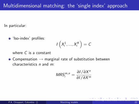
In particular:
�Iso-index�pro�les:I�X 1i , ...,X
Ki
�= C
where C is a constant
Compensation ! marginal rate of substitution betweencharacteristics n and m:
MRSm,ni =∂I/∂X n
∂I/∂Xm
P.A. Chiappori, Columbia () Matching modelsCemmap Masterclass, March 2011 7 /
22

Multidimensional matching: the �single index�approach
�Fully summarized�?
The joint density dµ�X 1, ...,XK ,Y 1, ...,Y L
�of observables among
married couples has the form:
dµ�X 1, ...,XK ,Y 1, ...,Y L
�= dν
hI�X 1, ...,XK
�, J�Y 1, ...,Y L
�ifor some measure dν on R2. Therefore:
The conditional distribution of�Y 1, ...,Y L
�given
�X 1, ...,XK
�only
depends on the value I�X 1, ...,XK
�(and same for men)
�Iso-attractiveness�: same conditional distribution of spouse�scharacteristics ! �iso-index�
Here: the subindex I , which only depends on observables, is asu¢ cient statistic for the distribution of characteristics of a man�sspouse (and same for women)
P.A. Chiappori, Columbia () Matching modelsCemmap Masterclass, March 2011 8 /
22

Multidimensional matching: the �single index�approach
In particular, one can (ordinally) non parametrically identify attractivenessindices. Indeed, for any characteristic s of the wife:
EhY s j X 1i , ...,XKi
i= φs
hI�X 1i , ...,X
Ki
�ifor some function φs . Then:
�iso-index�or �iso-attractiveness�pro�les:
EhY s j X 1i , ...,XKi
i= C 0
marginal rate of substitution between characteristics n and m:
MRSm,ni =∂I/∂X n
∂I/∂Xm=
∂E�Y s j X 1i , ...,XKi
�/∂X n
∂E�Y s j X 1i , ...,XKi
�/∂Xm
,
Over identifying restrictions: does not depend on s
Works for any moment
P.A. Chiappori, Columbia () Matching modelsCemmap Masterclass, March 2011 9 /
22
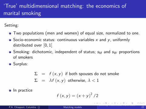
�True�multidimensional matching: the economics ofmarital smoking
Setting:
Two populations (men and women) of equal size, normalized to one.
Socio-economic status: continuous variables x and y , uniformlydistributed over [0, 1]
Smoking: dichotomic, independent of status; sM and sW proportionsof smokers
Surplus:
Σ = f (x , y) if both spouses do not smoke
Σ = λf (x , y) otherwise, λ < 1
In practicef (x , y) = (x + y)2 /2
P.A. Chiappori, Columbia () Matching modelsCemmap Masterclass, March 2011 10 /
22

�True�multidimensional matching: the economics ofmarital smoking
Basic remark:
The �twisted�condition does not hold.
Woman, index x0, non smoker:
∂xΣ = (x0 + y1) if she marries a non smoker with index y1∂xΣ = λ (x0 + y2) if she marries a smoker with index y2.
For any y2 2h(1�λ)x0
λ , 1i, if y1 = λy2 � (1� λ) x0, then the couples
(x0, y1) and (x0, y2) violate the twisted buyer condition; works for an openset of values x0 - namely x0 2
�0, λ1�λ
�.
Consequence:
The stable matching may not be pure.
P.A. Chiappori, Columbia () Matching modelsCemmap Masterclass, March 2011 11 /
22

�True�multidimensional matching: the economics ofmarital smoking
Particular case: if sM = sW then:
All smoking women marry smoking men, and conversely
All non smoking women marry non smoking men, and conversely
In words:
Even if λ very close to 1, fully discriminated submarkets
But: in practice,sM > sW
P.A. Chiappori, Columbia () Matching modelsCemmap Masterclass, March 2011 12 /
22

Main result
Proposition
Assume that λ � sMsM+1
. There exists four values X ,Y ,Y 0 and p, allbetween 0 and 1, such that:
For all x � X, a non-smoking woman with index x is matched withprobability 1 to a non-smoking husband with index
y =1� sW1� sM
x � sM � sW1� sM
� Y
and a smoking woman with index x is matched with probability 1 to asmoking husband with index
y 0 =sWsMx +
sM � sWsM
� Y 0
In particular, smoking men and non smoking women marry �down�,whereas non-smoking men and smoking women marry �up�.
P.A. Chiappori, Columbia () Matching modelsCemmap Masterclass, March 2011 13 /
22
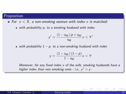
PropositionFor x < X, a non-smoking woman with index x is matched:
with probability p, to a smoking husband with index
y 0 =(1� sW ) p + sW
sMx < Y 0
with probability 1� p, to a non-smoking husband with index
y =(1� sW ) (1� p)
1� sMx < Y
Moreover, for any �xed index x of the wife, smoking husbands have ahigher index than non smoking ones - i.e., y 0 > y.
P.A. Chiappori, Columbia () Matching modelsCemmap Masterclass, March 2011 14 /
22

PropositionFor x < X, a smoking woman with index x is matched withprobability 1 to a smoking husband with index:
y 0 =(1� sW ) p + sW
sMx < Y 0
Finally, there are no couples in which the wife smokes and thehusband does not.
P.A. Chiappori, Columbia () Matching modelsCemmap Masterclass, March 2011 15 /
22

Women Men
X
Y
Y’
NS NSS S

0.0 0.1 0.2 0.3 0.4 0.5 0.6 0.7 0.8 0.9 1.00.0
0.1
0.2
0.3
0.4
0.5
0.6
0.7
0.8
0.9
x
u
Female utility (dashed = non smokers); sM = .25, sW = .2,λ = .8
P.A. Chiappori, Columbia () Matching modelsCemmap Masterclass, March 2011 17 /
22

0.0 0.1 0.2 0.3 0.4 0.5 0.6 0.7 0.8 0.9 1.00.0
0.1
0.2
0.3
0.4
0.5
0.6
0.7
0.8
0.9
1.0
y
v
Male utility (dashed = non smokers); sM = .25, sW = .2,λ = .8
P.A. Chiappori, Columbia () Matching modelsCemmap Masterclass, March 2011 18 /
22

Predictions
Non smoking husbands always marry a non smoking wife
Smoking husbands with a higher index (y 0 � Y 0) marry a high index,smoking wife with probability 1
Smoking husbands with a lower index (y 0 < Y 0) marry either asmoking or a non smoking wife with positive probability; moreover,both potential wives have the same quality index.
Similarly:
Smoking wifes always marry a smoking husband
Non smoking wifes with a higher index (x � X ) marry a high index,non smoking husband with probability 1
Non smoking wifes with a lower index (x < X ) marry either a smokingor a non smoking husband with positive probability; moreover, thesmoking husband is of higher quality than the non smoker.
P.A. Chiappori, Columbia () Matching modelsCemmap Masterclass, March 2011 19 /
22
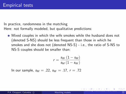
Empirical tests
In practice, randomness in the matchingHere: not formally modeled, but qualitative predictions:
Mixed couples in which the wife smokes while the husband does not(denoted S-NS) should be less frequent than those in which hesmokes and she does not (denoted NS-S) - i.e., the ratio of S-NS toNS-S couples should be smaller than:
r =sW (1� sM )sM (1� sW )
In our sample, sM = .22, sW = .17, r = .72
P.A. Chiappori, Columbia () Matching modelsCemmap Masterclass, March 2011 20 /
22

Empirical tests
Among couples with identical smoking habits, assortative matchingon socioeconomic status.
Non-smoking wives married with a smoking husband have a lowersocioeconomic status than those married with a non-smoking husband
Smoking husband married with a non-smoking wife have a lowersocioeconomic status than those married with a smoking wife.
When two (non smoking) women with the same (low) index marryrespectively a smoker and a non smoker, the non smoker should onaverage be of lower status than the smoker. In practice, smoking isnegatively correlated with status, especially for men. Still, we predictthat controlling for the wife�s �quality�, the smoking habit of thehusband should be less negatively correlated with his status.
P.A. Chiappori, Columbia () Matching modelsCemmap Masterclass, March 2011 21 /
22

Empirical results
P.A. Chiappori, Columbia () Matching modelsCemmap Masterclass, March 2011 22 /
22

II. Recently married: marital duration ≤ 4 years
Non-Smoking Wife Smoking Wife Non-Smoking Husband
71.66%
6.88%
Smoking Husband
12.17%
9.29%
Table A7: Observed Matching Husband’s age 24-36, Wife’s age 22-34. PSID 1999-2007. Weighed % I. Full sample
Non-Smoking Wife Smoking Wife
Non-Smoking Husband
74.74%
5.03%
Smoking Husband
11.43%
8.80%

Table 5: Sorting by education Husband’s age 24-34, Wife’s age 22-32. CPS 1996–2007. Both Non-Smokers Both Smokers
Wife’s
Education Husband’s Education
Wife’s Education
Husband’s Education
Spouse’s Education 0.633*** 0.694*** 0.458*** 0.442*** (0.013) (0.014) (0.035) (0.034) N 8710 8710 1150 1150 R2 0.47 0.47 0.27 0.28
Smoking Husband &
Non-Smoking Wife
Non-Smoking Husband &
Smoking Wife
Wife’s
Education Husband’s Education
Wife’s Education
Husband’s Education
Spouse’s Education 0.600*** 0.618*** 0.495*** 0.497*** (0.031) (0.036) (0.044) (0.041) N 1408 1408 767 767 R2 0.43 0.44 0.34 0.33 Note: All regressions include: own age, year and state fixed effects. Reference categories: 2007 and District of Columbia. Sampling weights are used. Robust standard errors. *** p-value < 0.01, ** p-value < 0.05, * p-value < 0.1

Table 6: Regression of Education by Smoking Status on Spouse’s Education and Smoking Behavior Husband’s age 24-34, Wife’s age 22-32. CPS 1996–2007. Wife’s Education Husband’s Education Non-Smoker Smoker Non-Smoker Smoker Spouse’s Education 0.630*** 0.473*** 0.684*** 0.556*** (0.012) (0.027) (0.013) (0.026) Spouse Smokes −0.141** −0.025 −0.209*** 0.160** (0.060) (0.086) (0.074) (0.076) N 10118 1917 9477 2558 R2 0.47 0.29 0.46 0.36 Note: All regressions include: own age, year and state fixed effects. Reference categories: 2007 and District of Columbia. Sampling weights are used. Robust standard errors. *** p-value < 0.01, ** p-value < 0.05, * p-value < 0.1

Table 7: Regression of Smoking Status on Education Husband’s age 24-34, Wife’s age 22-32. CPS 1996–2007. Men with NS Women Women with S Men (1) (2) (3) (4) Own Education −0.028*** −0.024*** −0.021*** −0.029*** (0.002) (0.002) (0.006) (0.007)
Test of Equality 0.0146 0.0341 (p-value)
Spouse’s Education -- −0.006** -- 0.014** (0.002) (0.006) N 10118 10118 2558 2558 R2 0.05 0.05 0.06 0.06 Note: All regressions include: own age, year and state fixed effects. Reference categories: 2007 and District of Columbia. Sampling weights are used. Robust standard errors. *** p-value < 0.01, ** p-value < 0.05, * p-value < 0.1

Table 8: Regression of Educational Difference on Smoking Status Men aged 24-34, Women aged 22-32. CPS 1996–2007.
ΔE = (Wife’s Education –
Husband’s Education)I(ΔE > 0)
Smoking Wife 0.341 0.157* (0.338) (0.090) Smoking Husband 0.819** 0.263*** (0.337) (0.089) Non-Smoking Wife × Non-Smoking Husband 0.476 0.185** (0.331) (0.088) Smoking Wife × Smoking Husband −0.659* −0.204** (0.351) (0.093) Mean of the dependent variable 0.17 0.31 N 12,035 12,035 R2 0.02 0.32 Note: All regressions include: wife’s age, husband’s age, year and state fixed effects. Reference categories: 2007 and District of Columbia. Sampling weights are used. Robust standard errors. *** p-value < 0.01, ** p-value < 0.05, * p-value < 0.1