Matching Weightsto Simultaneously Compare Three Treatment Groups:

a Simulation Study

Kazuki Yoshida, MD, MPH, MS*,

Sonia Hernandez-Dıaz, MD, DrPH, Daniel H. Solomon, MD, MPH,John W. Jackson, ScD, Joshua J. Gagne, PharmD, ScD,

Robert Glynn, PhD, Jessica M. Franklin, PhD

*Joint Doctor of Science StudentDepartments of Epidemiology & BiostatisticsHarvard T.H. Chan School of Public Health

677 Huntington Ave, Boston, MA 02115, USA

Last updated on June 22, 2016

Motivation

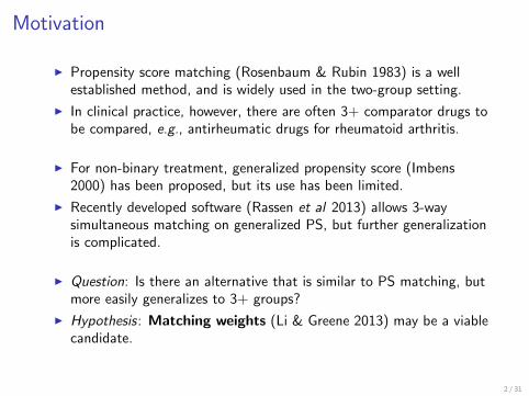
I Propensity score matching (Rosenbaum & Rubin 1983) is a wellestablished method, and is widely used in the two-group setting.

I In clinical practice, however, there are often 3+ comparator drugs tobe compared, e.g., antirheumatic drugs for rheumatoid arthritis.

I For non-binary treatment, generalized propensity score (Imbens2000) has been proposed, but its use has been limited.

I Recently developed software (Rassen et al 2013) allows 3-waysimultaneous matching on generalized PS, but further generalizationis complicated.

I Question: Is there an alternative that is similar to PS matching, butmore easily generalizes to 3+ groups?

I Hypothesis: Matching weights (Li & Greene 2013) may be a viablecandidate.

2 / 31

Matching weights definition

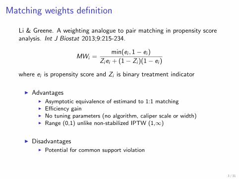
Li & Greene. A weighting analogue to pair matching in propensity scoreanalysis. Int J Biostat 2013;9:215-234.

MWi =min(ei , 1− ei )

Ziei + (1− Zi )(1− ei )

where ei is propensity score and Zi is binary treatment indicator

I AdvantagesI Asymptotic equivalence of estimand to 1:1 matchingI Efficiency gainI No tuning parameters (no algorithm, caliper scale or width)I Range (0,1) unlike non-stabilized IPTW (1,∞)

I DisadvantagesI Potential for common support violation

3 / 31

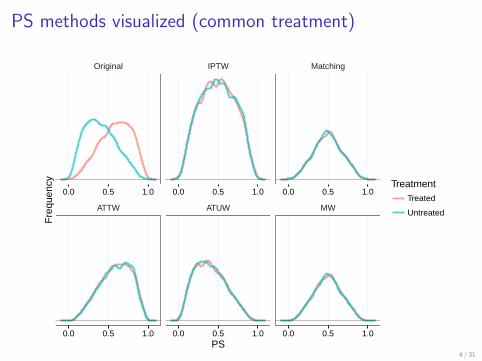
PS methods visualized (common treatment)

Original IPTW Matching

ATTW ATUW MW

0.0 0.5 1.0 0.0 0.5 1.0 0.0 0.5 1.0

0.0 0.5 1.0 0.0 0.5 1.0 0.0 0.5 1.0PS

Fre

quen

cy TreatmentTreated

Untreated

4 / 31

Comparing weighting methods

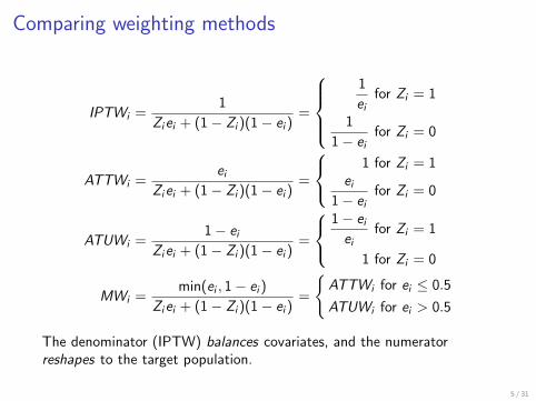
IPTWi =1

Ziei + (1− Zi )(1− ei )=

1

eifor Zi = 1

1

1− eifor Zi = 0

ATTWi =ei

Ziei + (1− Zi )(1− ei )=

1 for Zi = 1ei

1− eifor Zi = 0

ATUWi =1− ei

Ziei + (1− Zi )(1− ei )=

1− eiei

for Zi = 1

1 for Zi = 0

MWi =min(ei , 1− ei )

Ziei + (1− Zi )(1− ei )=

{ATTWi for ei ≤ 0.5

ATUWi for ei > 0.5

The denominator (IPTW) balances covariates, and the numeratorreshapes to the target population.

5 / 31

Extension of MW to K groupsI Define a propensity score (eki ) for each treatment category

(k ∈ {1, 2}) and redefine the treatment variable as Zi ∈ {1, 2}.

MWi =min(e1i , e2i )2∑

k=1

I (Zi = k)eki

=Smallest PS

PS of assigned treatment

I Use multinomial logistic regression for PS modelI Each subject has K propensity scores {e1i , e2i , ..., eKi}I K propensity scores sum to 1I Generalize the weights as

MWi =min(e1i , . . . , eKi )K∑

k=1

I (Zi = k)eki

6 / 31

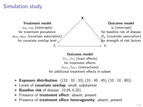
Simulation study

Ti

Xi

Yi

Outcome modelβT1, βT2 (main effects)

for treatment effectsβXT1, βXT2 (interactions)

for additional treatment effects in subset

Treatment modelα10, α20 (intercepts)

for treatment prevalenceα1X ,α2X (covariate association)

for covariate overlap level

Outcome modelβ0 (intercept)

for baseline risk of diseaseβX (covariate association)for strength of risk factors

I Exposure distribution: {(33 : 33 : 33), (10 : 45 : 45), (10 : 10 : 80)}I Levels of covariate overlap: small, substantialI Baseline risk of disease: {0.05, 0.20}I Presence of treatment effect: absent, presentI Presence of treatment effect heterogeneity: absent, present

7 / 31

Good overlap Poor overlap

●

●

●

●●

● ●

●●

●●

● ●

● ●

●●

● ●

●●

● ●

●

0

2000

4000

6000

U M Mw Ip U M Mw Ip

pExpo 33:33:33 10:45:45 10:10:80

Sample Sizes

X1 X4 X7

●

● ● ●

●

●● ●

●

●● ●

●

●●

●

●●

●

●

●●

●

●

● ● ●

●

●● ●

●

●● ●

●

●●

●

●

●●

●

●

●●

●

●

● ● ●

●

●● ●

●

●● ●

●

●●

●

●●

●

●

●●

●

0.0

0.1

0.2

0.3

0.4

0.5

0.0

0.1

0.2

0.3

0.4

0.5

Good overlap

Poor overlap

U M Mw Ip U M Mw Ip U M Mw Ipmethod

pExpo 33:33:33 10:45:45 10:10:80

Average Standardized Mean Differences

Modification (−)

1v0

Modification (−)

2v0

Modification (−)

2v1

Modification (+)

1v0

Modification (+)

2v0

Modification (+)

2v1

0.75

1.00

1.50

2.00

3.00

0.75

1.00

1.50

2.00

3.00

0.75

1.00

1.50

2.00

3.00

0.75

1.00

1.50

2.00

3.00

Null m

ain effectsN

ull main effects

Non−

null main effects

Non−

null main effects

Good overlap

Poor overlap

Good overlap

Poor overlap

U M Mw Ip U M Mw Ip U M Mw Ip U M Mw Ip U M Mw Ip U M Mw Ip

pExpo 33:33:33 10:45:45 10:10:80

pDis 0.05 0.2

Bias (Estimated Risk Ratio / True Risk Ratio)

Modification (−)

1v0

Modification (−)

2v0

Modification (−)

2v1

Modification (+)

1v0

Modification (+)

2v0

Modification (+)

2v1

●●●

●●●

●●● ●●●

●●● ●

●

●

●●●

●

●

●

●●●

●●●

●●●

●●●

●●● ●

●●

●●●

●

●

●

●●● ●●●

●●● ●●●

●

●

●

●

●

●●

●

●

●

●

●

●●● ●●●

●●● ●●●

●

●

●

●

●

●

●

●

●

●

●

●

●●● ●●●

●●● ●●●

●

●●

●

●

●

●●● ●●

●

●●● ●●●

●●● ●●●

●

●●

●

●

●

●●● ●

●

●

●●●

●●●

●●●

●●●

●●●

●

●●

●●●

●

●

●

●●●

●●●

●●●

●●●

●●●

●

●

●

●●●

●

●

●

●●● ●●●

●●● ●●●

●

●

●

●

●

●●

●●

●

●

●

●●● ●●●

●●● ●●●

●

●●

●

●

●

●

●

●

●

●

●

●●● ●●●

●●● ●●●

●●●

●

●

●

●●●●●

●

●●● ●●●

●●● ●●●

●●● ●

●

●

●●●

●●

●

0.0

0.5

1.0

1.5

0.0

0.5

1.0

1.5

0.0

0.5

1.0

1.5

0.0

0.5

1.0

1.5

Null m

ain effectsN

ull main effects

Non−

null main effects

Non−

null main effects

Good overlap

Poor overlap

Good overlap

Poor overlap

U M Mw Ip U M Mw Ip U M Mw Ip U M Mw Ip U M Mw Ip U M Mw Ip

pExpo 33:33:33 10:45:45 10:10:80

pDis ● 0.05 0.2

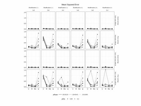
Mean Squared Error

Simulation: Summary results

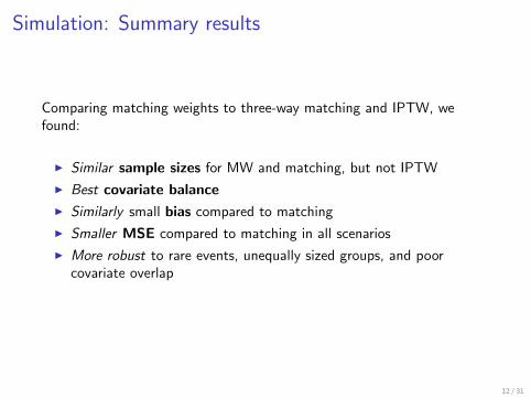
Comparing matching weights to three-way matching and IPTW, wefound:

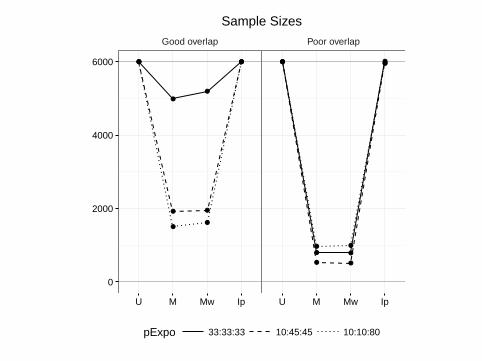
I Similar sample sizes for MW and matching, but not IPTW

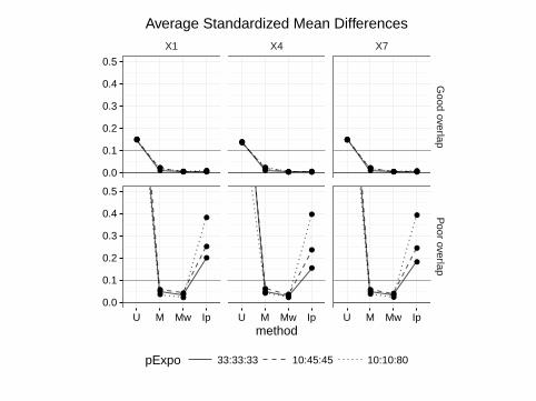
I Best covariate balance

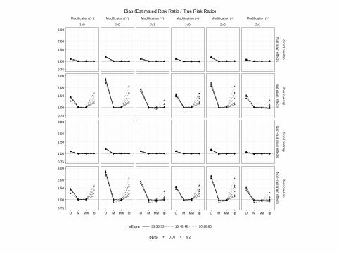
I Similarly small bias compared to matching

I Smaller MSE compared to matching in all scenarios

I More robust to rare events, unequally sized groups, and poorcovariate overlap

12 / 31

Conclusion

I MW has been suggested as a more efficient alternative to 1:1pairwise matching with a similar estimand (Li & Greene 2013).

I In the three treatment group setting, MW demonstrated similar bias,but smaller MSE compared to 1:1:1 three-way matching in asimulation study.

I Efficiency gain compared to 1:1:1 three-way matching was morenoticeable in scenarios in which the outcome events were rare,treatment groups were unequally sized, or covariate overlap waspoor.

I Compared to IPTW, MW was more stable in the poor covariateoverlap setting.

13 / 31

Acknowledgment

KY currently receives tuition support jointly from Japan StudentServices Organization (JASSO) and Harvard T. H. Chan School ofPublic Health (partially supported by training grants from Pfizer,Takeda, Bayer and PhRMA).

14 / 31

Additional slides with details follow

15 / 31

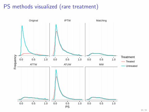
PS methods visualized (rare treatment)

Original IPTW Matching

ATTW ATUW MW

0.0 0.5 1.0 0.0 0.5 1.0 0.0 0.5 1.0

0.0 0.5 1.0 0.0 0.5 1.0 0.0 0.5 1.0PS

Fre

quen

cy TreatmentTreated

Untreated

16 / 31

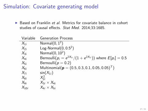
Simulation: Covariate generating model

I Based on Franklin et al. Metrics for covariate balance in cohortstudies of causal effects. Stat Med. 2014;33:1685.

Variable Generation ProcessX1i Normal(0, 12)X2i Log-Normal(0, 0.52)X3i Normal(0, 102)X4i Bernoulli(pi = e2X1i/(1 + e2X1i )) where E [pi ] = 0.5X5i Bernoulli(p = 0.2)X6i Multinomial(p = (0.5, 0.3, 0.1, 0.05, 0.05)T )X7i sin(X1i )X8i X 2

2i

X9i X3i × X4i

X10i X4i × X5i

17 / 31

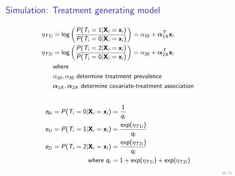
Simulation: Treatment generating model

ηT1i = log

(P(Ti = 1|Xi = xi )

P(Ti = 0|Xi = xi )

)= α10 + αT

1Xxi

ηT2i = log

(P(Ti = 2|Xi = xi )

P(Ti = 0|Xi = xi )

)= α20 + αT

2Xxi

where

α10, α20 determine treatment prevalence

α1X ,α2X determine covariate-treatment association

e0i = P(Ti = 0|Xi = xi ) =1

qi

e1i = P(Ti = 1|Xi = xi ) =exp(ηT1i )

qi

e2i = P(Ti = 2|Xi = xi ) =exp(ηT2i )

qi

where qi = 1 + exp(ηT1i ) + exp(ηT2i )

18 / 31

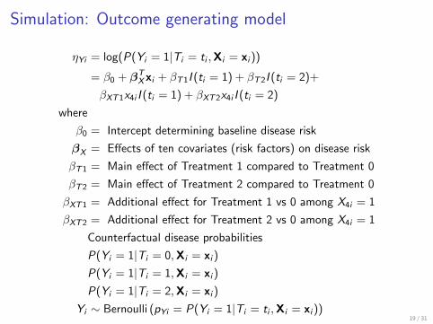
Simulation: Outcome generating model

ηYi = log(P(Yi = 1|Ti = ti ,Xi = xi ))

= β0 + βTX xi + βT1I (ti = 1) + βT2I (ti = 2)+

βXT1x4i I (ti = 1) + βXT2x4i I (ti = 2)

where

β0 = Intercept determining baseline disease risk

βX = Effects of ten covariates (risk factors) on disease risk

βT1 = Main effect of Treatment 1 compared to Treatment 0

βT2 = Main effect of Treatment 2 compared to Treatment 0

βXT1 = Additional effect for Treatment 1 vs 0 among X4i = 1

βXT2 = Additional effect for Treatment 2 vs 0 among X4i = 1

Counterfactual disease probabilities

P(Yi = 1|Ti = 0,Xi = xi )

P(Yi = 1|Ti = 1,Xi = xi )

P(Yi = 1|Ti = 2,Xi = xi )

Yi ∼ Bernoulli (pYi = P(Yi = 1|Ti = ti ,Xi = xi ))19 / 31

Simulation: Analyses

I All computation except 3-way matching was performed in R

I Multinomial logistic regression with all covariates as the propensityscore model.

I Matched analyses:I Three-way nearest neighbor algorithm implemented in the

pharmacoepi toolbox by Rassen et al generated matched “trios”.I Caliper for the matched trio triangle perimeter was defined as

0.6

√τ21+τ2

2+τ23

3where τ 2j = Var(e1|T=j)+Var(e2|T=j)

2.

I OLS linear regression was conducted in the matched dataset.

I Weighted analysis:I MW and stabilized IPTWI survey package was used to appropriately account for weighting in

the outcome log linear model.

20 / 31

Simulation: Assessment metrics

I Matched/weighted sample size

I Covariate standardized mean difference (SMD) averaged acrossthree contrasts

I bias in risk ratio

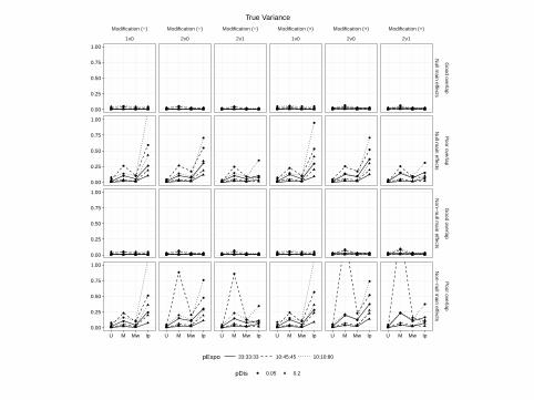
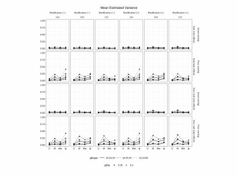
I Simulation and estimated variance of estimators

I Mean squared error of estimators

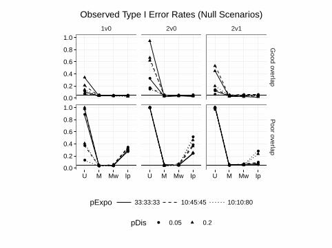
I False positive rates in null scenarios

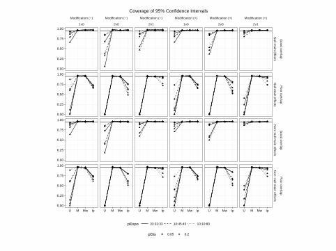
I Coverage probability of estimated confidence intervals

21 / 31

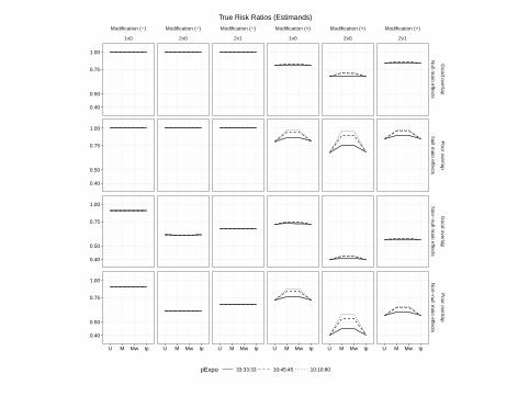
Modification (−)

1v0

Modification (−)

2v0

Modification (−)

2v1

Modification (+)

1v0

Modification (+)

2v0

Modification (+)

2v1

0.40

0.50

0.75

1.00

0.40

0.50

0.75

1.00

0.40

0.50

0.75

1.00

0.40

0.50

0.75

1.00

Null m

ain effectsN

ull main effects

Non−

null main effects

Non−

null main effects

Good overlap

Poor overlap

Good overlap

Poor overlap

U M Mw Ip U M Mw Ip U M Mw Ip U M Mw Ip U M Mw Ip U M Mw Ip

pExpo 33:33:33 10:45:45 10:10:80

True Risk Ratios (Estimands)

Modification (−)

1v0

Modification (−)

2v0

Modification (−)

2v1

Modification (+)

1v0

Modification (+)

2v0

Modification (+)

2v1

●●●

●●●

●●●

●●●

●●●

●

●

●

●

●●

●

●

●

●●●

●●●

●●●

●●●

●●●

●

●

●

●●●

●

●

●

●●● ●●●

●●● ●●●

●●●

●

●

●

●

●

●

●

●

●

●●● ●●●

●●● ●●●

●●●

●

●

●

●

●

●

●

●

●

●●● ●●●

●●● ●●●

●●●

●

●

●

●●● ●

●

●

●●● ●●●

●●● ●●●

●●●

●

●

●

●●● ●

●

●

●●●

●●●

●●●

●●●

●●●

●

●

●

●●●

●

●

●

●●●

●●●

●●●

●●●

●●●

●

●

●

●●●

●

●

●

●●● ●●●

●●● ●●●

●●●

●

●

●●

●

●

●

●

●

●●● ●●●

●●● ●●●

●●●

●

●

●

●

●

●

●

●

●

●●● ●●●

●●● ●●●

●●●

●

●

●

●●●

●

●

●

●●● ●●●

●●● ●●●

●●●

●

●

●

●●●

●

●

●

0.00

0.25

0.50

0.75

1.00

0.00

0.25

0.50

0.75

1.00

0.00

0.25

0.50

0.75

1.00

0.00

0.25

0.50

0.75

1.00

Null m

ain effectsN

ull main effects

Non−

null main effects

Non−

null main effects

Good overlap

Poor overlap

Good overlap

Poor overlap

U M Mw Ip U M Mw Ip U M Mw Ip U M Mw Ip U M Mw Ip U M Mw Ip

pExpo 33:33:33 10:45:45 10:10:80

pDis ● 0.05 0.2

True Variance

Modification (−)

1v0

Modification (−)

2v0

Modification (−)

2v1

Modification (+)

1v0

Modification (+)

2v0

Modification (+)

2v1

●●●

●●●

●●●

●●●

●●●

●

●

●

●●●

●

●

●

●●●

●●●

●●●

●●●

●●●

●

●

●

●●●

●

●

●

●●● ●●●

●●● ●●●

●●●

●

●

●

●

●

●

●

●●

●●● ●●●

●●● ●●●

●●●

●

●

●

●

●

●●

●●

●●● ●●●

●●● ●●●

●●●

●

●

●

●●● ●●

●

●●● ●●●

●●● ●●●

●●●

●

●

●

●●●

●●

●

●●●

●●●

●●●

●●●

●●●

●

●

●

●●●

●

●

●

●●●

●●●

●●●

●●●

●●●

●

●

●

●●●

●

●

●

●●● ●●●

●●● ●●●

●●●

●

●

●

●

●

●

●●●

●●● ●●●

●●● ●●●

●●●

●

●

●

●

●

●

●

●●

●●● ●●●

●●● ●●●

●●●

●

●

●

●●● ●

●

●

●●● ●●●

●●● ●●●

●●●

●

●

●

●●● ●

●

●

0.00

0.25

0.50

0.75

1.00

0.00

0.25

0.50

0.75

1.00

0.00

0.25

0.50

0.75

1.00

0.00

0.25

0.50

0.75

1.00

Null m

ain effectsN

ull main effects

Non−

null main effects

Non−

null main effects

Good overlap

Poor overlap

Good overlap

Poor overlap

U M Mw Ip U M Mw Ip U M Mw Ip U M Mw Ip U M Mw Ip U M Mw Ip

pExpo 33:33:33 10:45:45 10:10:80

pDis ● 0.05 0.2

Mean Estimated Variance

Modification (−)

1v0

Modification (−)

2v0

Modification (−)

2v1

Modification (+)

1v0

Modification (+)

2v0

Modification (+)

2v1

●●

●

●●

●

●●

●

●

●●

●

●●

●

●●

●●

●

●●

●

●●

●

●

●

●

●

●

●

●

●

●

●●●

●●●

●●●

●

●

●

●

●

●

●

●

●

●●●

●●●

●●●

●

●

●●

●

●

●

●

●

●●

●●●●

●●

●

●

●●

●

●●

●

●●

●●

●●●

●●●

●

●

●●

●

●●

●

●

●

●●

●

●●

●

●●

●

●

●●

●

●●

●

●●

●●

●

●●

●

●●

●

●

●

●

●

●

●

●

●

●

●●●

●●●

●●●

●

●

● ●

●

● ●

●

●

●●●

●●●

●●●

●

●

●●

●

●

●

●

●

●●

●

●●

●●●

●

●

●●

●

●●

●

●●

●●

●●●

●●●

●

●

●

●

●

●

●

●

●

●

0.00

0.05

0.10

0.15

0.20

0.25

0.00

0.05

0.10

0.15

0.20

0.25

0.00

0.05

0.10

0.15

0.20

0.25

0.00

0.05

0.10

0.15

0.20

0.25

Null m

ain effectsN

ull main effects

Non−

null main effects

Non−

null main effects

Good overlap

Poor overlap

Good overlap

Poor overlap

Est. True Boot. Est. True Boot. Est. True Boot. Est. True Boot. Est. True Boot. Est. True Boot.

pExpo 33:33:33 10:45:45 10:10:80

pDis ● 0.05 0.2

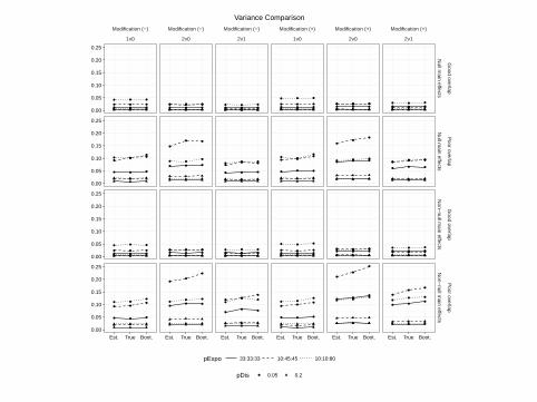
Variance Comparison

1v0 2v0 2v1

●●● ●●● ●●● ●●●

●

●

●

●●● ●●●

●

●●

●

●●

●●● ●●● ●●●

●●●

●●● ●●●

●

●

●

●●

● ●●● ●●● ●●●

●●●

●●● ●●● ●●

●

0.0

0.2

0.4

0.6

0.8

1.0

0.0

0.2

0.4

0.6

0.8

1.0

Good overlap

Poor overlap

U M Mw Ip U M Mw Ip U M Mw Ip

pExpo 33:33:33 10:45:45 10:10:80

pDis ● 0.05 0.2

Observed Type I Error Rates (Null Scenarios)

Modification (−)

1v0

Modification (−)

2v0

Modification (−)

2v1

Modification (+)

1v0

Modification (+)

2v0

Modification (+)

2v1

●●●

●●● ●●● ●●●

●

●

●

●●● ●●●

●

●

●

●●●

●●● ●●● ●●●

●

●

●

●●● ●●●

●

●

●

●

●●

●●● ●●● ●●●

●●●

●●● ●●●

●

●

●

●

●●

●●● ●●● ●●●

●●●

●●● ●●●

●

●

●

●●

● ●●● ●●● ●●●

●●●

●●● ●●● ●●

●

●●●

●●● ●●● ●●●

●●

●

●●● ●●● ●●

●

●●● ●●● ●●● ●●●

●

●

●

●●● ●●●

●

●

●

●●● ●●● ●●● ●●●

●

●

●

●●● ●●●

●

●

●

●●●

●●● ●●● ●●●

●●●

●●● ●●●

●

●

●

●●●

●●● ●●● ●●●

●●●

●●● ●●●

●

●

●

●●● ●●● ●●● ●●●

●

●

●

●●● ●●●●●

●

●●● ●●● ●●● ●●●

●

●

●

●●● ●●●

●●

●

0.00

0.25

0.50

0.75

1.00

0.00

0.25

0.50

0.75

1.00

0.00

0.25

0.50

0.75

1.00

0.00

0.25

0.50

0.75

1.00

Null m

ain effectsN

ull main effects

Non−

null main effects

Non−

null main effects

Good overlap

Poor overlap

Good overlap

Poor overlap

U M Mw Ip U M Mw Ip U M Mw Ip U M Mw Ip U M Mw Ip U M Mw Ip

pExpo 33:33:33 10:45:45 10:10:80

pDis ● 0.05 0.2

Coverage of 95% Confidence Intervals

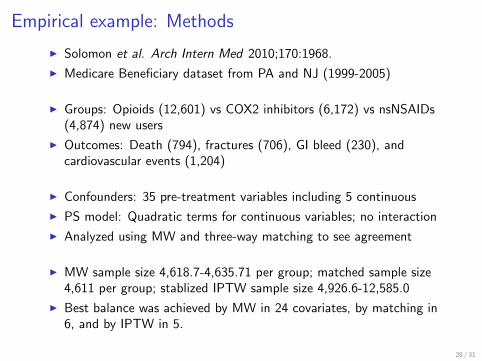
Empirical example: Methods

I Solomon et al. Arch Intern Med 2010;170:1968.

I Medicare Beneficiary dataset from PA and NJ (1999-2005)

I Groups: Opioids (12,601) vs COX2 inhibitors (6,172) vs nsNSAIDs(4,874) new users

I Outcomes: Death (794), fractures (706), GI bleed (230), andcardiovascular events (1,204)

I Confounders: 35 pre-treatment variables including 5 continuous

I PS model: Quadratic terms for continuous variables; no interaction

I Analyzed using MW and three-way matching to see agreement

I MW sample size 4,618.7-4,635.71 per group; matched sample size4,611 per group; stablized IPTW sample size 4,926.6-12,585.0

I Best balance was achieved by MW in 24 covariates, by matching in6, and by IPTW in 5.

28 / 31

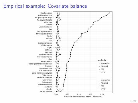
Empirical example: Covariate balance

●

●

●

●

●

●

●

●

●

●

●

●

●

●

●

●

●

●

●

●

●

●

●

●

●

●

●

●

●

●

●

●

●

●

●

Hepatic diseaseGender

ARB useAlzheimer disease

OsteoporosisHypertension

Parkinson's diseaseThiazide use

Bone meneral density testACE inhibitor useAntiepileptic use

DiabetesUpper gastrointestinal disease

HyperlipidemiaGout

Benzodiazepine useBeta blocker use

Back painSSRI use

AnginaH2 blocker use

Corticosteroid useFalls

PPI useStroke

Myocardial infarctionNo. physician visits

AgeLoop diuretic use

FractureWhite race

No. days in hospitalNo. prescription drugs

Antithrombotic useCharlson score

0.00 0.05 0.10 0.15 0.20Absolute Standardized Mean Difference

Methods● Unmatched

Matched

MW

IPTW

Unmatched

Matched

MW

IPTW

29 / 31

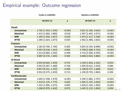
Empirical example: Outcome regression

Yoshida K et al. Matching Weights for Three-category Exposure 2/9/2016

- 1 -

Table 1. Comparison of hazard ratios for coxibs and opioids (nonselective NSAIDs as the reference)

by different methods and outcomes.

Coxibs vs nsNSAIDs

Opioids vs nsNSAIDs

HR [95% CI] p

HR [95% CI] p

Death

Unmatched 1.702 [1.293, 2.240] <0.001 2.821 [2.185, 3.642] <0.001 Matched 1.415 [1.060, 1.889] 0.018 1.997 [1.492, 2.671] <0.001 MW 1.393 [1.056, 1.837] 0.019 1.973 [1.517, 2.566] <0.001 IPTW 1.385 [1.024, 1.873] 0.035 1.962 [1.480, 2.601] <0.001

Fracture

Unmatched 1.181 [0.799, 1.746] 0.405 5.825 [4.195, 8.089] <0.001 Matched 0.947 [0.618, 1.453] 0.804 4.708 [3.308, 6.702] <0.001 MW 1.013 [0.684, 1.502] 0.948 4.733 [3.396, 6.595] <0.001 IPTW 0.887 [0.576, 1.365] 0.585 4.068 [2.814, 5.882] <0.001

GI bleed

Unmatched 0.933 [0.605, 1.439] 0.753 1.529 [1.034, 2.262] 0.033 Matched 0.932 [0.587, 1.480] 0.766 1.005 [0.615, 1.643] 0.984 MW 0.857 [0.551, 1.335] 0.496 1.108 [0.737, 1.668] 0.622 IPTW 0.916 [0.575, 1.459] 0.713 1.196 [0.793, 1.804] 0.394

Cardiovascular

Unmatched 1.603 [1.298, 1.979] <0.001 2.294 [1.882, 2.797] <0.001 Matched 1.419 [1.135, 1.775] 0.002 1.585 [1.255, 2.003] <0.001 MW 1.355 [1.096, 1.675] 0.005 1.626 [1.326, 1.995] <0.001 IPTW 1.268 [0.979, 1.642] 0.072 1.445 [1.125, 1.856] 0.004

Abbreviations: MW: matching weights; IPTW: inverse probability of treatment weights; Matched:

three-way matching; Coxibs: COX-2 selective inhibitors; nsNSAIDs: non-selective non-steroidal

anti-inflammatory drugs; HR: hazard ratio; CI: confidence interval.

Table 1

30 / 31

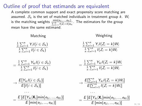
Outline of proof that estimands are equivalentA complete common support and exact propensity score matching areassumed. Sk is the set of matched individuals in treatment group k. Wi

is the matching weights min(e1i ,...,eKi )∑Kk=1 I (Zi=k)eki

. The estimators for the group

mean have the same estimand.

Matching

1n

∑ni=1 Yi I (i ∈ Sk)

1n

∑ni=1 I (i ∈ Sk)

=1n

∑ni=1 Yki I (i ∈ Sk)

1n

∑ni=1 I (i ∈ Sk)

→ E [Yki I (i ∈ Sk)]

E [I (i ∈ Sk)]

. . .

=E [E [Yki |Xi ]min(e1i , ..., eKi )]

E [min(e1i , ..., eKi )]

Weighting

1n

∑ni=1 Yi I (Zi = k)Wi

1n

∑ni=1 I (Zi = k)Wi

=1n

∑ni=1 Yki I (Zi = k)Wi

1n

∑ni=1 I (Zi = k)Wi

→E [∑n

i=1 Yki I (Zi = k)Wi ]

E [∑n

i=1 I (Zi = k)Wi ]

. . .

=E [E [Yki |Xi ]min(e1i , ..., eKi )]

E [min(e1i , ..., eKi )] 31 / 31