material and capacity requirements planning with dynamic

HAL Id: hal-00724885https://hal.archives-ouvertes.fr/hal-00724885

Submitted on 23 Aug 2012

HAL is a multi-disciplinary open accessarchive for the deposit and dissemination of sci-entific research documents, whether they are pub-lished or not. The documents may come fromteaching and research institutions in France orabroad, or from public or private research centers.

L’archive ouverte pluridisciplinaire HAL, estdestinée au dépôt et à la diffusion de documentsscientifiques de niveau recherche, publiés ou non,émanant des établissements d’enseignement et derecherche français ou étrangers, des laboratoirespublics ou privés.

Material and Capacity Requirements Planning withdynamic lead times.

Herbert Jodlbauer, Sonja Reitner

To cite this version:Herbert Jodlbauer, Sonja Reitner. Material and Capacity Requirements Planning with dy-namic lead times.. International Journal of Production Research, Taylor & Francis, 2011, pp.1.�10.1080/00207543.2011.603707�. �hal-00724885�

https://hal.archives-ouvertes.fr/hal-00724885

https://hal.archives-ouvertes.fr

For Peer Review O

nly

Material and Capacity Requirements Planning with dynamic

lead times.

Journal: International Journal of Production Research

Manuscript ID: TPRS-2010-IJPR-0906.R2

Manuscript Type: Original Manuscript

Date Submitted by the Author:

24-May-2011

Complete List of Authors: Jodlbauer, Herbert; FH-Studiengange Steyr, Operations Management Reitner, Sonja; FH-Studiengaenge Steyr, Operations Management

Keywords: MRP, CAPACITY PLANNING

Keywords (user): Material requirements planning, Dynamic lead times

http://mc.manuscriptcentral.com/tprs Email: [email protected]

International Journal of Production Research

For Peer Review O

nly

1

Material and Capacity Requirements Planning with dynamic lead

times

Herbert Jodlbauer*, Sonja Reitner

Department of Operations Management, Upper Austrian University of Applied

Sciences, Steyr, Austria

Wehrgrabengasse 1-3, 4400 Steyr, Austria, Tel.: +43 (0)7252 884-3810, Fax.: -3199

(Received XX Month Year; final version received XX Month Year)

Traditional MRP does not consider the finite capacity of machines and assumes fixed

lead times. This paper develops an approach (MCRP) to integrating capacity planning

into material requirements planning. To get a capacity feasible production plan different

measures for capacity adjustment such as alternative routeings, safety stock, lot splitting

and lot summarization are discussed. Additionally, lead times are no longer assumed to

be fixed. They are calculated dynamically with respect to machine capacity utilisation. A

detailed example is presented to illustrate how the MCRP approach works successfully.

Keywords: MRP, Material Requirements Planning, capacity planning, dynamic lead times

1. Introduction

Conventional enterprise resource planning (ERP) material planning methods are

based on material requirements planning (MRP), a production planning system

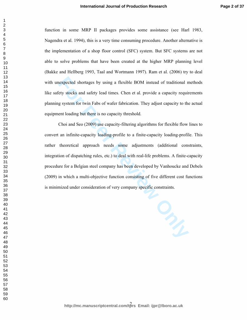
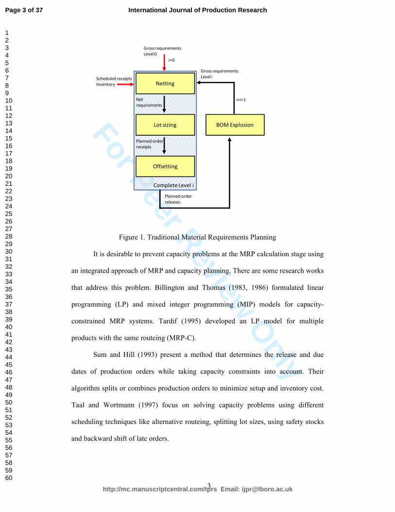
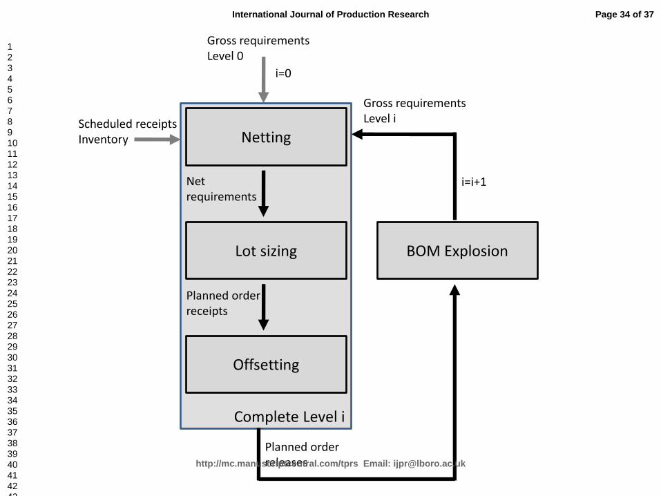
developed by Orlicky (1975). The MRP steps for each level in the bill of material

(BOM), beginning with the end items, are netting, lot sizing, offsetting and the BOM

explosion (see Figure 1). Two of the most important weak points of MRP are the

assumptions of infinite machine capacity and of production lead times which are

constant or depend on lot size, processing and setup time. In practice, lead times

depend on many factors such as machine utilization, lot size, inventory and

dispatching rules and are thus variable. Kanet (1986) shows that using fixed lead

times results in over-planning of inventory at every level.

Ignoring finite machine capacity leads to capacity infeasible schedules which

have to be revised by the user. Although the capacity requirements planning (CRP)

* Corresponding author. E-mail address: [email protected]

Page 1 of 37



123456789101112131415161718192021222324252627282930313233343536373839404142434445464748495051525354555657585960

For Peer Review O

nly

2

function in some MRP II packages provides some assistance (see Harl 1983,

Nagendra et al. 1994), this is a very time consuming procedure. Another alternative is

the implementation of a shop floor control (SFC) system. But SFC systems are not

able to solve problems that have been created at the higher MRP planning level

(Bakke and Hellberg 1993, Taal and Wortmann 1997). Ram et al. (2006) try to deal

with unexpected shortages by using a flexible BOM instead of traditional methods

like safety stocks and safety lead times. Chen et al. provide a capacity requirements

planning system for twin Fabs of wafer fabrication. They adjust capacity to the actual

equipment loading but there is no capacity threshold.

Choi and Seo (2009) use capacity-filtering algorithms for flexible flow lines to

convert an infinite-capacity loading-profile to a finite-capacity loading-profile. This

rather theoretical approach needs some adjustments (additional constraints,

integration of dispatching rules, etc.) to deal with real-life problems. A finite-capacity

procedure for a Belgian steel company has been developed by Vanhoucke and Debels

(2009) in which a multi-objective function consisting of five different cost functions

is minimized under consideration of very company specific constraints.

Page 2 of 37



123456789101112131415161718192021222324252627282930313233343536373839404142434445464748495051525354555657585960

For Peer Review O

nly

3

Netting

Lot sizing BOM Explosion

Offsetting

Gross requirements

Level 0

Gross requirements

Level i

i=i+1Net

requirements

i=0

Planned order

receipts

Planned order

releases

Scheduled receipts

Inventory

Complete Level i

Figure 1. Traditional Material Requirements Planning

It is desirable to prevent capacity problems at the MRP calculation stage using

an integrated approach of MRP and capacity planning. There are some research works

that address this problem. Billington and Thomas (1983, 1986) formulated linear

programming (LP) and mixed integer programming (MIP) models for capacity-

constrained MRP systems. Tardif (1995) developed an LP model for multiple

products with the same routeing (MRP-C).

Sum and Hill (1993) present a method that determines the release and due

dates of production orders while taking capacity constraints into account. Their

algorithm splits or combines production orders to minimize setup and inventory cost.

Taal and Wortmann (1997) focus on solving capacity problems using different

scheduling techniques like alternative routeing, splitting lot sizes, using safety stocks

and backward shift of late orders.

Page 3 of 37



123456789101112131415161718192021222324252627282930313233343536373839404142434445464748495051525354555657585960

For Peer Review O

nly

4

Pandey et al. (2000) point out that complex algorithms are often not easily

understood by the planner and so they have developed a less mathematically

complicated system for finite capacity MRP (FCMRP), which is executed in two

stages. First, capacity-based production schedules are generated and then, in a second

step, the algorithm produces an appropriate material requirements plan to satisfy the

schedules obtained from the first stage. The model is restricted to lot for lot as the

only possible lot sizing rule and there is a single resource for each part type.

Wuttipornpun and Yenradee (2004) study a FCMRP system where they use a

variable lead time for MRP depending on the lot size, processing and setup time.

After scheduling jobs they reduce capacity problems by using alternative machines if

possible and adjusting the timing of jobs (starting the jobs earlier or delaying them).

Limitations of this model are: Bottleneck machines produce only one part, lot-for-lot

is the only lot sizing rule which is allowed and there is no overlap of production

batches. A further development of this approach is TOC-MRP (Wuttipornpun and

Yenradee 2007). With similar limitations the TOC philosophy is adopted in FCMRP

which results in a better performance compared to FCMRP.

Commercially available FCMRP software uses two different approaches for

including finite capacity: pre/post-MRP analysis and finite capacity scheduling

(Nagendra and Das 2001). Neither of them resolves the capacity problem during the

MRP run itself. Additionally computational effort increases substantially and so Lee

et al. (2009) proposed parallelising the MRP process and using a computational grid

which can exploit idle computer capacity.

Kanet and Stößlein (2010) describe ‘Capacitated ERP’ (CERP) – a variation

of MRP that takes resource capacity into account before exploding requirements to

Page 4 of 37



123456789101112131415161718192021222324252627282930313233343536373839404142434445464748495051525354555657585960

For Peer Review O

nly

5

lower level components. The model is limited to one-stage production, single-level

BOM, single resource and no backorders.

The main approaches of MRP and capacity planning are summarized in Table

1. As you can see, considering finite capacity in Material Requirements Planning is an

old issue in production research but one which has not yet been solved satisfactorily.

Theoretical scheduling algorithms cause high calculating times for real word

problems and are not easy for planners to understand. MRP-CRP, MRP-SFC and

FCMRP approaches are also very time-consuming and attempt to solve the capacity

problem after an MRP run. Research contributions which try to integrate capacity

constraints into MRP are often limited to simple production environments.

Table 1. Main approaches of MRP and finite capacity planning

Approach References Limitations

Traditional MRP Orlicky (1975) fixed lead times, infinite capacity

MRP- CRP Harl (1983) identification of capacity problems after an MRP run, considerable participation of planner is

necessary

MRP-SFC Taal and

Wortmann (1997)

capacity problems are not solved on MRP level

FCMRP Pandey et al.

(2000)

capacity problems are not solved on MRP level,

lot sizing: only lot-for-lot, single resource for

each part type

Wuttipornpun and

Yenradee (2004)

capacity problems are not solved on MRP level,

lot sizing: only lot-for-lot, bottleneck machine:

one part type

Finite capacity

scheduling algorithms

Choi and Seo

(2009)

flexible flow line, theoretical approach,

constraints for real-life problems are missing

Vanhoucke and

Debels (2009)

company specific constraints

MRP and

integrated capacity

planning

Billington and

Thomas (1983)

mathematical programming formulation of the

problem, high computational effort for real-life

problems

Tardif (1995) same routeing for all products

Sum and Hill

(1993)

capacity-sensitive lot sizing with complex

algorithms (not easy for planners to understand,

high computational effort for real-life problems)

Taal and

Wortmann (1997)

fixed lead times

Kanet and

Stößlein (2010)

one-stage production, single-level BOM, single

resource, no backorders

Page 5 of 37



123456789101112131415161718192021222324252627282930313233343536373839404142434445464748495051525354555657585960

For Peer Review O

nly

6

This paper aims to modify traditional MRP in two directions:

(1) by integrating capacity planning in the MRP run at each level in the BOM.

(2) by using variable lead times

For capacity adjustment, different measures like alternative routeings, safety stocks,

adjusting lot sizes and adding capacity are applied in a predefined sequence. Lead

times are not predefined fixed parameters. They are calculated dynamically,

dependent on lot sizes, inventory and required machine capacity. The presented

approach can handle multiple products, multiple resources, multi-stage production

and multi-level BOM. There is no restriction concerning the lot sizing rule. As in

traditional MRP all lot sizing rules can be used. An advantage of this approach in

practice is that it is based on the well-known MRP methodology. Dynamic lead times

and finite capacity are integrated at every stage of the MRP run to reduce the

shortcomings of MRP.

The paper is organized as follows. The integration of capacity planning is described in

Section 2, where each step is explained in detail. Section 3 illustrates the approach

with a numerical example. The conclusions are stated in Section 4.

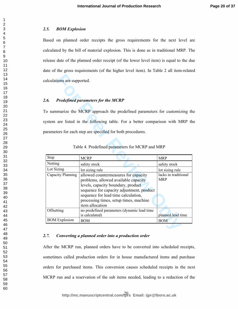
2. Integrating capacity planning into the concept of MRP

In this section the basic ideas of integrating capacity requirements planning as well as

capacity adjustment into material requirements planning (MRP) are presented.

In the traditional MRP approach the items in the bill of material (BOM) are

sorted in levels according to the rule that items consist only of items from a higher

level, whereby end items (that are not part of any other items) are placed at level 0

(low level code). In Figure 2 the steps of Material and Capacity Requirements

Page 6 of 37



123456789101112131415161718192021222324252627282930313233343536373839404142434445464748495051525354555657585960

For Peer Review O

nly

7

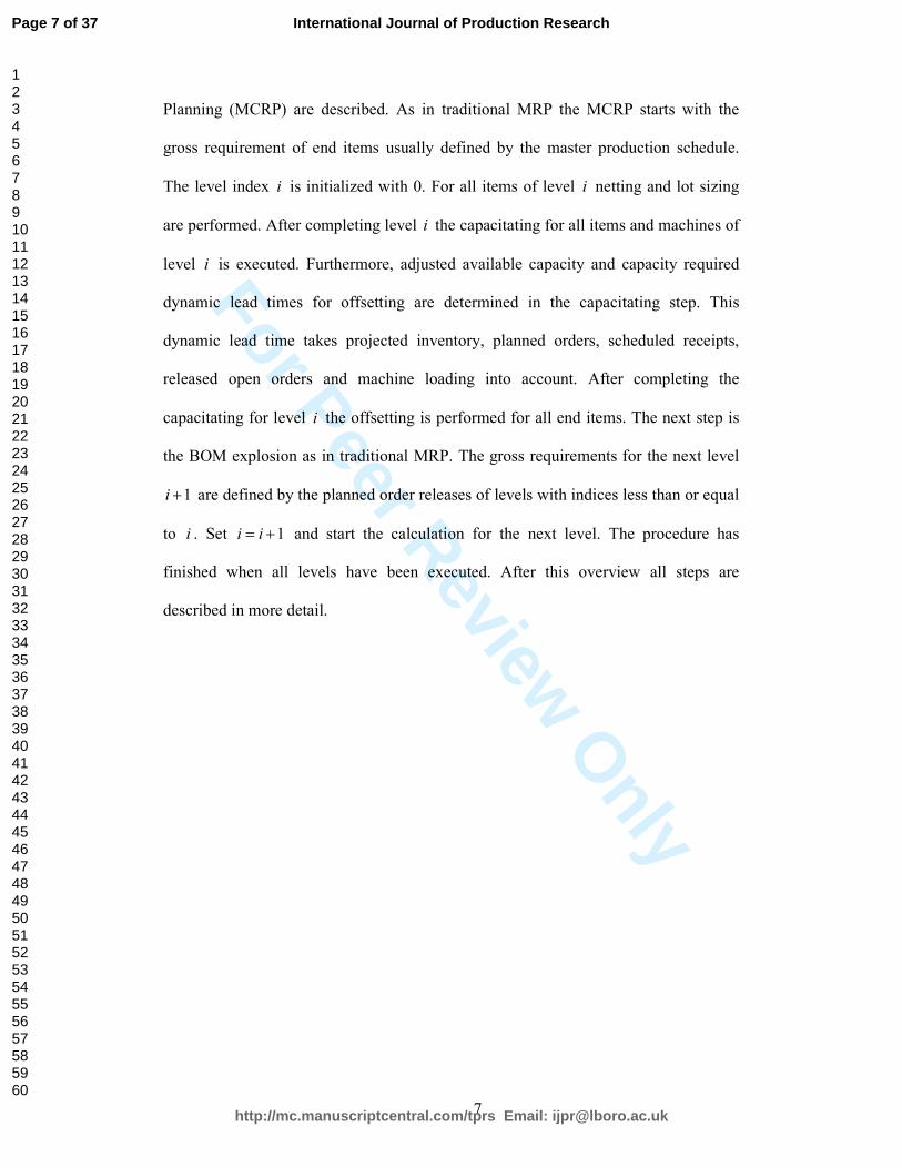
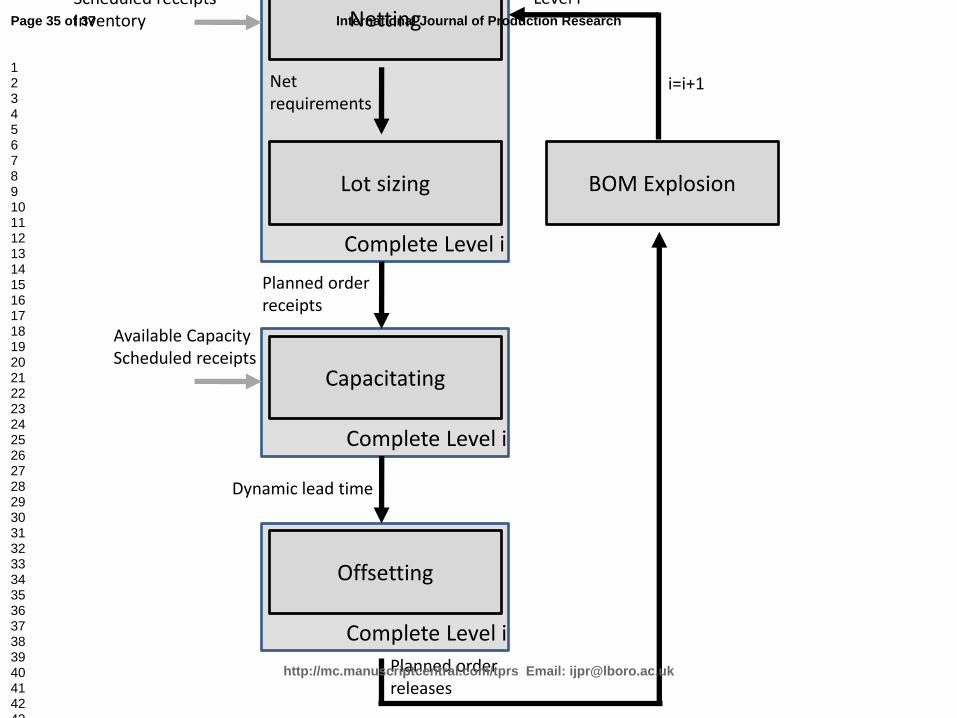
Planning (MCRP) are described. As in traditional MRP the MCRP starts with the

gross requirement of end items usually defined by the master production schedule.

The level index i is initialized with 0. For all items of level i netting and lot sizing

are performed. After completing level i the capacitating for all items and machines of

level i is executed. Furthermore, adjusted available capacity and capacity required

dynamic lead times for offsetting are determined in the capacitating step. This

dynamic lead time takes projected inventory, planned orders, scheduled receipts,

released open orders and machine loading into account. After completing the

capacitating for level i the offsetting is performed for all end items. The next step is

the BOM explosion as in traditional MRP. The gross requirements for the next level

1+i are defined by the planned order releases of levels with indices less than or equal

to i . Set 1= +i i and start the calculation for the next level. The procedure has

finished when all levels have been executed. After this overview all steps are

described in more detail.

Page 7 of 37



123456789101112131415161718192021222324252627282930313233343536373839404142434445464748495051525354555657585960

For Peer Review O

nly

8

Netting


Offsetting

Gross requirements

Level 0

Gross requirements

Level i

i=i+1Net

requirements

i=0

Planned order

receipts

Planned order

releases

Scheduled receipts

Inventory

Complete Level i

Capacitating

Dynamic lead time

Complete Level i

Complete Level i

Available Capacity

Scheduled receipts

Figure 2. Material and Capacity Requirements Planning (MCRP)

2.1. Netting

In the netting step, the net requirements are determined by taking into account the

gross requirements, scheduled receipts and inventory. The gross requirements for the

end items are predefined by the master production schedule. The gross requirements

for sub items are set by the bill of material explosion during MCRP. Scheduled

receipts are converted to planned order receipts and may be released or not released to

production. Sub items needed for scheduled receipts are allocated in stock or taken

from stock. Netting is performed as in traditional MRP. Net requirements are

calculated under consideration of projected inventory, safety stock and gross

requirements. A more sophisticated approach can take dynamic planned safety stocks

Page 8 of 37



123456789101112131415161718192021222324252627282930313233343536373839404142434445464748495051525354555657585960

For Peer Review O

nly

9

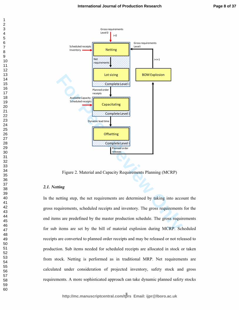
into account as Kanet et al. (2010) suggest in their work. Netting is supported by

Table 2.

Table 2. MCRP table for one item

Period 1 2 3 4 5 6 7 8 9 …

Gross requirements from MPS or see BOM explosion

Scheduled receipts see convert an order

Projected inventory see netting

Net requirement see netting

Planned order receipts see lot sizing

Calculated lead time ( ),j kl see capacity planning

Planned order releases see offsetting

2.2. Lot sizing

To trade off changeover cost against holding cost a lot sizing rule is applied. In this

approach all known lot sizing methods for MRP can be applied. If there are no

essential changeover costs or if enough excess capacity is available the Lot for Lot

strategy is recommended to reduce inventory (see Haddock and Hubicky 1989). In all

other cases dynamic rules, for instance Groff (see Groff 1979) or Fixed Order Period

(see Hopp and Spearman 2008) should be applied. The results of the lot sizing are the

due dates for the planned orders and the batch size of the orders (the two are called

planned order receipts). A planned order receipt of 10 items in period 5 means, that it

is planned to finish 10 items by the end of period 5. Lot sizing is also supported by

Table 2.

2.3. Capacity planning

This step is compared to MRP new and is applied for all items manufactured in-

house. Purchased parts, for which subcontracting in the sense of capacity buying is

performed, can be treated as parts manufactured in-house, whereby information of the

available capacity from the supplier is necessary. All other purchased items are

Page 9 of 37



123456789101112131415161718192021222324252627282930313233343536373839404142434445464748495051525354555657585960

For Peer Review O

nly

10

treated with predefined planned lead times as in traditional MRP (and no capacity

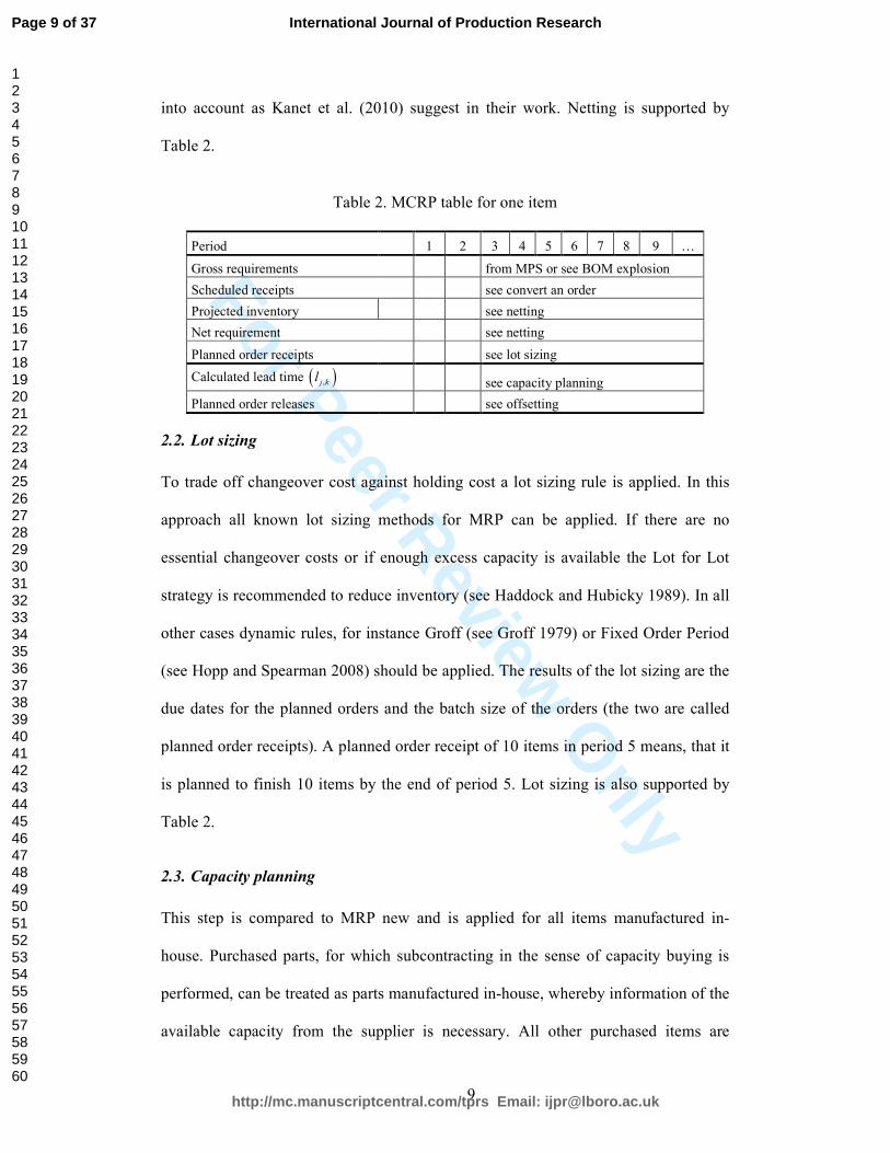
planning is performed). The capacity planning consists of two main steps: capacity

adjustment and calculation of the dynamic lead time and the release dates.

2.3.1. Capacity adjustment

The available capacity is based on shift models, working time and number of workers

and may be adjusted. Scheduled receipts are determined by the number of items and a

due date. The required capacity for scheduled receipts can be calculated under

consideration of lot sizes, processing times and set up times and will be referred to as

scheduled capacity receipts. In analogy the required capacities of planned order

receipts are referred to as planned capacity receipts. The cumulated values are

calculated by the sum over the time periods. The cumulated required capacity is

defined as the sum of the cumulated scheduled capacity receipts and the cumulated

planned capacity receipts. The free cumulated capacity is the difference between the

cumulated available capacity and the cumulated required capacity and must be non-

negative to ensure capacity feasibility. The calculation is supported by Table 3, the

explanation of the capacity envelope follows in the chapter 2.3.2.

Table 3. MCRP table for one capacity group

Period 1 2 3 4 5 6 7 8 9 …

Available capacity

Scheduled capacity receipts ( )capSR

Planned capacity receipts ( )capPO

Cumulated available capacity ( )ia

Cumulated required capacity ( )ir

Free cumulated capacity ( )−i ia r

Capacity envelope ( )ie

Page 10 of 37



123456789101112131415161718192021222324252627282930313233343536373839404142434445464748495051525354555657585960

For Peer Review O

nly

11

If the planned capacity receipts are higher than the net available capacity this is not

necessarily a reason for a capacity infeasible schedule because the scheduled capacity

receipts as well as the planned capacity receipts allocate the whole required capacity

to the due date (but it may be produced in earlier periods). To achieve capacity

feasibility, the cumulated available capacity must be high enough to cover the

cumulated required capacity.

If the cumulated required capacity is higher than the cumulated available

capacity, there is a capacity problem and no capacity feasible production schedule can

be found (see Hübl et al. 2009). The following countermeasures can be considered:

(1) Alternative routeings

(2) Relaxing safety stocks

(3) Applying lot splitting with consecutive processing

(4) Applying lot summarization

(5) Adjusting available capacity by adding capacity (over time, more staff, etc.)

(6) Accepting tardiness respectively by backlog or postponing gross requirement

in the master plan

The first measure for decreasing required capacity is choosing alternative routings

(see Taal and Wortmann 1997). Production orders, planned on the bottleneck resource

in overloaded periods, should be planned on alternative resources if it is possible to

unload the bottleneck resource. If the capacity of alternative resources is short, lot

splitting with simultaneous processing using alternative resources is suggested.

Measures (2), (3) and (4) require starting the netting and lot sizing with

changed parameters on the current level. For the further discussion let T be the latest

period at which a capacity problem is given (i. e. cumulated required capacity is

higher than the cumulated available capacity).

Page 11 of 37



123456789101112131415161718192021222324252627282930313233343536373839404142434445464748495051525354555657585960

For Peer Review O

nly

12

Relaxing safety stock is a measure which is also proposed by Taal and

Wortmann (1997) but with a lower priority than is used in this approach. It can easily

be performed by running the netting and lot sizing with safety stocks equal to zero as

long as the net requirements have an influence on the capacity problem. More

accurately, all net requirements which are combined to planned order receipts with

due dates before or equal to T should be calculated assuming safety stock to be zero.

All others should be calculated with the predefined safety stock. This postponement

can solve or improve the capacity problem, reduce the inventory and increase the

danger of stock outs because of unforeseen events (machine breakdown, scrap,

rework, demand fluctuation, etc.).

Lot splitting with consecutive processing is very useful if only short or no set

up time is required and net requirements of more than one period are combined to one

batch. To execute lot splitting, lot sizing is based on an adjusted rule for all batches

which combine net requirements with due dates before T and with due dates after T.

All these batches are divided into two lots. The first lot combines all net requirements

with due dates earlier than or equal to T and the second the remaining net

requirements. The second batch should be planned as late as possible to reduce

inventory. Lot splitting can solve or improve the capacity problem, reduce inventory

and increase change over costs.

Lot summarization can be useful if there is an essential change over time and

the same item is planned in different orders, all with due dates before T. In this case

all planned orders with due dates before or equal to T are combined to one new

planned order receipt. Lot summarization can solve or improve the capacity problem,

increase inventory and reduce changeover costs.

Page 12 of 37



123456789101112131415161718192021222324252627282930313233343536373839404142434445464748495051525354555657585960

For Peer Review O

nly

13

If the first four mentioned measures do not solve the capacity problem,

additional capacity (e.g. over time, more staff, additional shift, etc.) is needed within

the allowed and possible capacity boundaries. In general, this measure should solve

the capacity problem or the capacity problem has to be accepted, resulting in backlog.

Of course additional costs are thereby incurred.

If all measures do not solve the capacity problem, tardiness of at least one job

has to be accepted. In order to ensure a consistent procedure a reduction or a

postponement of gross requirements in the master plan is recommended whereby it is

necessary to start the whole procedure again at level zero. One way to find suitable

master plan orders (for reduction or postponement) is to apply pegging (see Hopp and

Spearman 2008). The following steps have to be performed: Step 1: Searching the due

date T1 of master plan orders which lies the furthermost in the future and is connected

with a planned order at the current level whose due date is earlier than or equal to T.

Step 2: Select master plan orders with due dates before T1 which are not important

(e.g. a stock order, customer acceptance of later delivery date, bad contribution

margin and no strategically unimportant order from a C customer, etc.) and in which

required capacity at the current level is greater than the missed capacity, and postpone

them until after T1 or delete them.

For the capacity adjustment a specific product sequence is defined. Depending

on the importance of different managerial goals, one of the following proposed

criteria can be chosen to build up the sequence.

• importance of service level (starting with the item with the least important

service level)

• holding cost (starting with the item with the highest holding cost per unit)

Page 13 of 37



123456789101112131415161718192021222324252627282930313233343536373839404142434445464748495051525354555657585960

For Peer Review O

nly

14

For measures (2) and (3) the sequence should be applied as defined above. For

measure (4) the sequence of the service level and the holding cost criteria should be

applied in the reversed order.

The described measures for capacity adjustment are applied in the order in

which they are listed above and for the products in the predefined sequence. If the

capacity problem is solved, then the capacity adjustment procedure has to be stopped.

If the measures applied to the current level do not lead to capacity feasibility, the

measures can be applied to lower levels. After applying these measures, we assume

that the cumulated required capacity is less than the cumulated available capacity.

Furthermore, if possible (e.g. at the end of the planning horizon) the available

capacity should be reduced.

2.3.2. Calculation of dynamic lead times and release dates

Now the second step in capacity planning is performed. This is the calculation of the

dynamic lead times and the release dates. The lead time calculation is based on a

predefined product sequence, starting with the item which should be produced as late

as possible. This can be a different sequence to the one used for capacity adjustment.

In order to build up the sequence one of the following criteria can be used:

• holding cost (starting with the item with the highest holding cost per unit)

This criterion reduces inventory holding costs.

• set up (starting with the item which should be produced last)

This criterion reduces changeover costs if set up times depend on the

sequence.

• tardiness (starting with the item with the lowest tardiness penalty cost)

This criterion reduces tardiness for items with the highest penalty costs.

Page 14 of 37



123456789101112131415161718192021222324252627282930313233343536373839404142434445464748495051525354555657585960

For Peer Review O

nly

15

The predefined sequence should be consistent over all levels supporting a first-in-

first-out principle along the routeing.

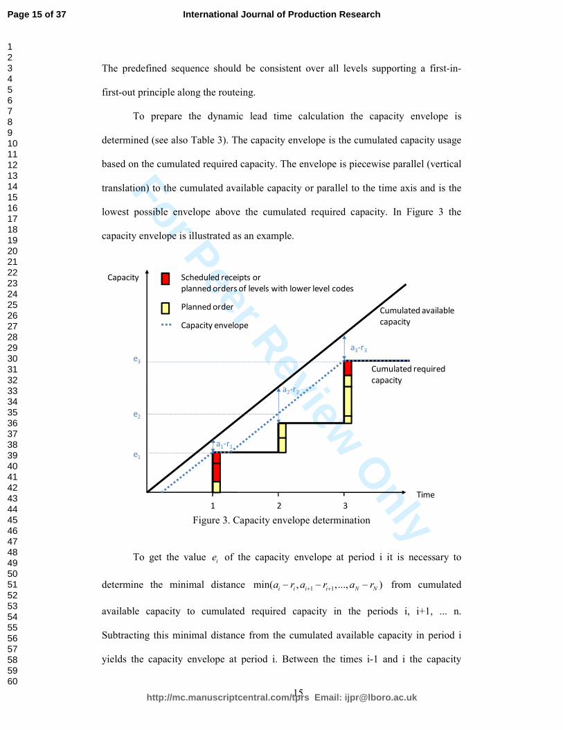
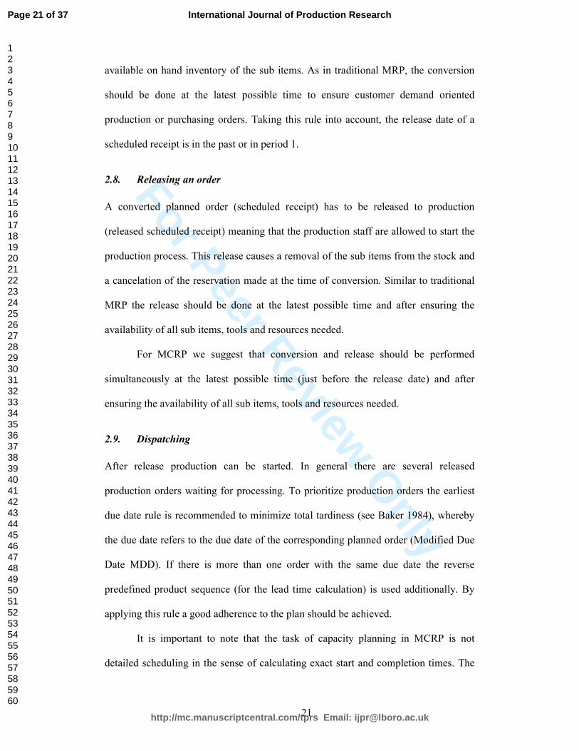
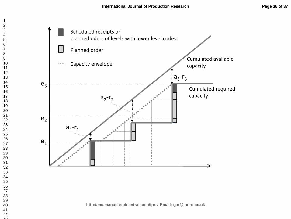
To prepare the dynamic lead time calculation the capacity envelope is

determined (see also Table 3). The capacity envelope is the cumulated capacity usage

based on the cumulated required capacity. The envelope is piecewise parallel (vertical

translation) to the cumulated available capacity or parallel to the time axis and is the

lowest possible envelope above the cumulated required capacity. In Figure 3 the

capacity envelope is illustrated as an example.

Scheduled receipts or

planned orders of levels with lower level codes

Planned order Cumulated available

capacity

Cumulated required

capacity

Capacity envelope

Capacity

Time

1 2 3

a1-r1

a2-r2

a3-r3

e2

e3

e1

Figure 3. Capacity envelope determination

To get the value ie of the capacity envelope at period i it is necessary to

determine the minimal distance 1 1min( , ,..., )+ +− − −i i i i N Na r a r a r from cumulated

available capacity to cumulated required capacity in the periods i, i+1, ... n.

Subtracting this minimal distance from the cumulated available capacity in period i

yields the capacity envelope at period i. Between the times i-1 and i the capacity

Page 15 of 37



123456789101112131415161718192021222324252627282930313233343536373839404142434445464748495051525354555657585960

For Peer Review O

nly

16

envelope is a piecewise linear function which is constant and equal to the value of the

capacity envelope in period i-1 or a linear function of which the slope is the difference

1−−i ia a between the cumulated available capacity values in period i and period i-1.

The major value of these two functions determines the value of the capacity envelope.

In the following formula the calculation of the envelope is defined.

( )( )( ) ] ]1 1

1 1

min( , ,..., )

( ) max , , for 1,

discrete time capacity envelope in period i

( ) continuous time capacity envelope with respect to time t

cumulated requi

i i i i i i N N

i i i i

i

i

e a a r a r a r

e t e e a a t i t i i

e

e t

r

+ +

− −

= − − − −

= + − − ∈ −

L

L

L red capacity in period i

cumulated available capacity in period i

number of periods in the planning horizon

ia

N

L

L

(1)

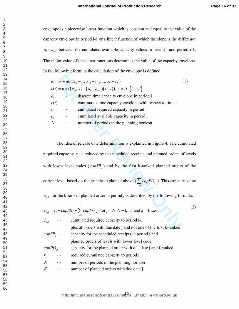
The idea of release date determination is explained in Figure 4. The cumulated

required capacity jr is reduced by the scheduled receipts and planned orders of levels

with lower level codes ( jcapSR ) and by the first k-ranked planned orders of the

current level based on the criteria explained above (1=

∑k

ji

i

capPO ). This capacity value

,j kc for the k-ranked planned order in period j is described by the following formula:

,

1

,

, for j , 1,...1 and 1,...

cumulated required capacity to period j-1

plus all orders with due date j and not one of the first k-ranked

capacity for the schedu

=

= − − = − =∑

L

L

k

j k j j ji j

i

j k

j

c r capSR capPO N N k K

c

capSR led receipts in period j and

planned orders of levels with lower level code

capacity for the planned order with due date j and i-ranked

required cumulated capacity to period j

number of per

L

L

L

ji

j

capPO

r

N iods in the planning horizon

number of planned orders with due date jLjK

(2)

Page 16 of 37



123456789101112131415161718192021222324252627282930313233343536373839404142434445464748495051525354555657585960

For Peer Review O

nly

17

Now the capacity value ,j kc is intersected with the capacity envelope ( )e t for

determining the lead time ,j kl and the release date ,j kt for the k-ranked planned order.

The next formula provides detailed information for calculating these two values.

,

,

1

, ,

,

,

,

calculated lead time of the k-ranked planned order with due date j

release date to the k-ranked planned order with due date j

cumulated required capacity to

j j k

j k

j j

j k j k

j k

j k

j k

e cl

a a

t j l

l

t

c

−

−=

−

= −

L

L

L period j-1

plus all orders with due date j and not one of the first k-ranked

cumulated available capacity to period j

capacity envelope in period j

j

j

a

e

L

L

(3)

Scheduled receipts or

planned orders of levels with lower level codes

Planned order

Cumulated required capacity

Capacity envelope

Capacity

Time1 2 3

c3,1

capSR3

capPO31

capPO32

capPO33

l3,1

t3,1

e3-c3,1

Release dates

e3

Figure 4. Release date determination

Page 17 of 37



123456789101112131415161718192021222324252627282930313233343536373839404142434445464748495051525354555657585960

For Peer Review O

nly

18

The determination of the lead time and the release date for the first-ranked order in

period 3 is visualized in Figure 4. For the release date calculation in the whole

planning horizon it is necessary to start at the furthermost future time period within

the planning horizon. If the release date of the first-ranked planned order of the last

period in the planning is determined, the capacity value is reduced by the next

planned order. This value is intersected with the capacity envelope and so on. If this

procedure is completed on the last due date, then the next earlier due date is chosen.

The scheduled capacity receipts are subtracted first and then the calculation of the

release date is performed with the predefined sequence again until all planned orders

are finished. The calculated lead time should be entered in Table 2. The release date

for the k-ranked planned order is the latest possible time when the available capacity

between the release date and the due date covers the capacity needed to produce the

first k-ranked planned orders as well as the scheduled receipts.

2.3.3. Building machine groups

The combination of several machines into one machine group is useful but

requires some adjustment of the calculation procedure for the dynamic lead time. If n

equivalent machines are combined into one group, the group available capacity is of

course the available capacity of the individual machine multiplied by n. But if an

order is produced only on one machine and is not split among several machines

simultaneously, the order processing time is not equal to required capacity over

available group capacity. We have to take into account the number of machines

combined into one machine group. Hence the correct calculation of the order

processing time is: order processing time is equal to required capacity multiplied by n

over available group capacity. Consequently, to determine the dynamic lead time for a

machine group the following steps should be performed:

Page 18 of 37



123456789101112131415161718192021222324252627282930313233343536373839404142434445464748495051525354555657585960

For Peer Review O

nly

19

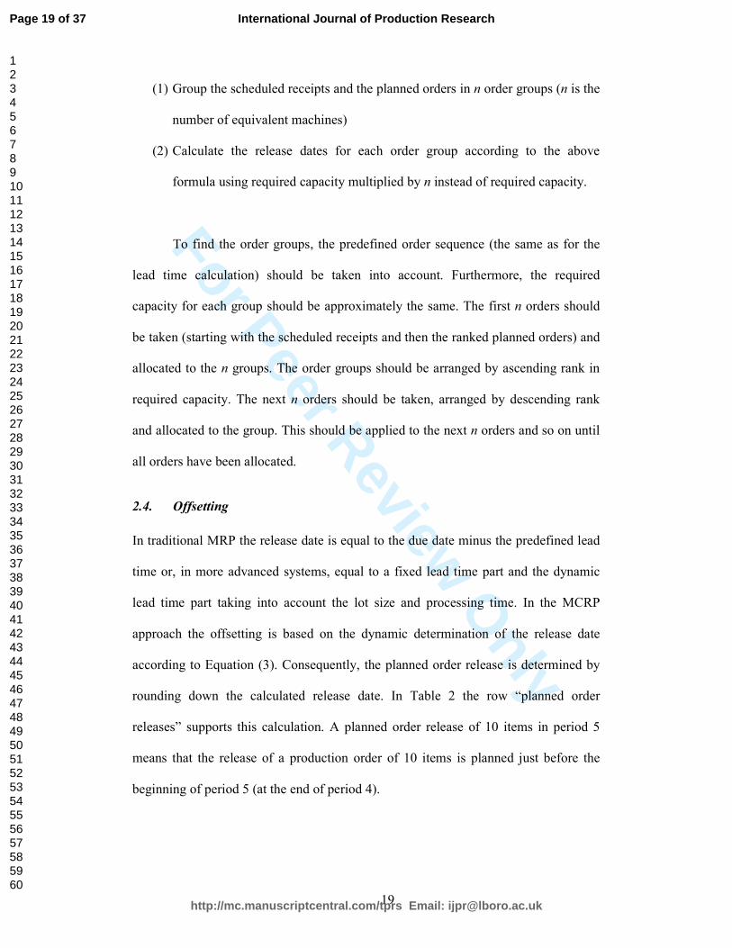
(1) Group the scheduled receipts and the planned orders in n order groups (n is the

number of equivalent machines)

(2) Calculate the release dates for each order group according to the above

formula using required capacity multiplied by n instead of required capacity.

To find the order groups, the predefined order sequence (the same as for the

lead time calculation) should be taken into account. Furthermore, the required

capacity for each group should be approximately the same. The first n orders should

be taken (starting with the scheduled receipts and then the ranked planned orders) and

allocated to the n groups. The order groups should be arranged by ascending rank in

required capacity. The next n orders should be taken, arranged by descending rank

and allocated to the group. This should be applied to the next n orders and so on until

all orders have been allocated.

2.4. Offsetting

In traditional MRP the release date is equal to the due date minus the predefined lead

time or, in more advanced systems, equal to a fixed lead time part and the dynamic

lead time part taking into account the lot size and processing time. In the MCRP

approach the offsetting is based on the dynamic determination of the release date

according to Equation (3). Consequently, the planned order release is determined by

rounding down the calculated release date. In Table 2 the row “planned order

releases” supports this calculation. A planned order release of 10 items in period 5

means that the release of a production order of 10 items is planned just before the

beginning of period 5 (at the end of period 4).

Page 19 of 37



123456789101112131415161718192021222324252627282930313233343536373839404142434445464748495051525354555657585960

For Peer Review O

nly

20

2.5. BOM Explosion

Based on planned order receipts the gross requirements for the next level are

calculated by the bill of material explosion. This is done as in traditional MRP. The

release date of the planned order receipt (of the lower level item) is equal to the due

date of the gross requirements (of the higher level item). In Table 2 all item-related

calculations are supported.

2.6. Predefined parameters for the MCRP

To summarize the MCRP approach the predefined parameters for customizing the

system are listed in the following table. For a better comparison with MRP the

parameters for each step are specified for both procedures.

Table 4. Predefined parameters for MCRP and MRP

Step MCRP MRP

Netting safety stock safety stock

Lot Sizing lot sizing rule lot sizing rule

Capacity Planning allowed countermeasures for capacity

problems, allowed available capacity

levels, capacity boundary, product

sequence for capacity adjustment, product

sequence for lead time calculation,

processing times, setup times, machine

item allocation

lacks in traditional

MRP

Offsetting no predefined parameters (dynamic lead time

is calculated) planned lead time

BOM Explosion BOM BOM

2.7. Converting a planned order into a production order

After the MCRP run, planned orders have to be converted into scheduled receipts,

sometimes called production orders for in house manufactured items and purchase

orders for purchased items. This conversion causes scheduled receipts in the next

MCRP run and a reservation of the sub items needed, leading to a reduction of the

Page 20 of 37



123456789101112131415161718192021222324252627282930313233343536373839404142434445464748495051525354555657585960

For Peer Review O

nly

21

available on hand inventory of the sub items. As in traditional MRP, the conversion

should be done at the latest possible time to ensure customer demand oriented

production or purchasing orders. Taking this rule into account, the release date of a

scheduled receipt is in the past or in period 1.

2.8. Releasing an order

A converted planned order (scheduled receipt) has to be released to production

(released scheduled receipt) meaning that the production staff are allowed to start the

production process. This release causes a removal of the sub items from the stock and

a cancelation of the reservation made at the time of conversion. Similar to traditional

MRP the release should be done at the latest possible time and after ensuring the

availability of all sub items, tools and resources needed.

For MCRP we suggest that conversion and release should be performed

simultaneously at the latest possible time (just before the release date) and after

ensuring the availability of all sub items, tools and resources needed.

2.9. Dispatching

After release production can be started. In general there are several released

production orders waiting for processing. To prioritize production orders the earliest

due date rule is recommended to minimize total tardiness (see Baker 1984), whereby

the due date refers to the due date of the corresponding planned order (Modified Due

Date MDD). If there is more than one order with the same due date the reverse

predefined product sequence (for the lead time calculation) is used additionally. By

applying this rule a good adherence to the plan should be achieved.

It is important to note that the task of capacity planning in MCRP is not

detailed scheduling in the sense of calculating exact start and completion times. The

Page 21 of 37



123456789101112131415161718192021222324252627282930313233343536373839404142434445464748495051525354555657585960

For Peer Review O

nly

22

objective is to support material requirements planning by ensuring capacity feasible

plans (because of the fact that cumulated available capacity is higher than cumulated

required capacity) and lowest possible inventory (because of shortest capacity feasible

lead times).

As a result of the planning procedure it may be possible that a production

order lies within another production order (release date A ≤ release date B ≤ due

date B ≤ due date A) with the same item produced. In this case the summarization of

the two orders is recommended.

2.10. Completing the order

After finishing an order the items should be booked to the inventory in real time and

the released scheduled receipt has to be deleted in real time. For orders which take a

long time it is useful to partly book the items to inventory and to simultaneously

reduce the scheduled receipts in order to ensure a realistic cumulated required

capacity. Backlog and orders which are late are added to the scheduled receipts in

period one.

3. Illustration of the concept

The following example is provided to show how the MCRP approach may be used. In

this example two end items A and B are considered. Item A consists of one item X

and one item Y. Item B is assembled from one item Y and one item Z. Table 5

delivers necessary input data for all items. The available capacity per period of the

two machines M0 and M1 is 420 TU. The predefined product sequence for capacity

adjustment and lead time calculation is A, B (for M0) and X, Y, Z (for M1).

Table 5. Input data for all items

Item A B X Y Z

Page 22 of 37



123456789101112131415161718192021222324252627282930313233343536373839404142434445464748495051525354555657585960

For Peer Review O

nly

23

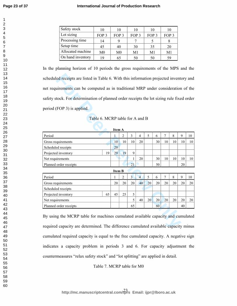
Safety stock 10 10 10 10 10

Lot sizing FOP 3 FOP 3 FOP 3 FOP 3 FOP 3

Processing time 14 9 7 5 8

Setup time 45 40 30 35 20

Allocated machine M0 M0 M1 M1 M1

On hand inventory 19 65 50 50 59

In the planning horizon of 10 periods the gross requirements of the MPS and the

scheduled receipts are listed in Table 6. With this information projected inventory and

net requirements can be computed as in traditional MRP under consideration of the

safety stock. For determination of planned order receipts the lot sizing rule fixed order

period (FOP 3) is applied.

Table 6. MCRP table for A and B

Item A

Period 1 2 3 4 5 6 7 8 9 10

Gross requirements 10 10 10 20

30 10 10 10 10

Scheduled receipts 20

Projected inventory 19 29 19 9

Net requirements 0 0 1 20 0 30 10 10 10 10

Planned order receipts 0 0 21 0 0 50 0 0 20 0

Item B

Period 1 2 3 4 5 6 7 8 9 10

Gross requirements 20 20 20 40 20 20 20 20 20 20

Scheduled receipts




By using the MCRP table for machines cumulated available capacity and cumulated

required capacity are determined. The difference cumulated available capacity minus

cumulated required capacity is equal to the free cumulated capacity. A negative sign

indicates a capacity problem in periods 3 and 6. For capacity adjustment the

countermeasures “relax safety stock” and “lot splitting” are applied in detail.

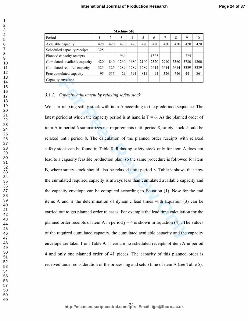
Table 7. MCRP table for M0

Page 23 of 37



123456789101112131415161718192021222324252627282930313233343536373839404142434445464748495051525354555657585960

For Peer Review O

nly

24

Machine M0

Period 1 2 3 4 5 6 7 8 9 10

Available capacity 420 420 420 420 420 420 420 420 420 420

Scheduled capacity receipts 325

Planned capacity receipts

964

1325

725

Cumulated available capacity 420 840 1260 1680 2100 2520 2940 3360 3780 4200

Cumulated required capacity 325 325 1289 1289 1289 2614 2614 2614 3339 3339

Free cumulated capacity 95 515 -29 391 811 -94 326 746 441 861

Capacity envelope

3.1.1. Capacity adjustment by relaxing safety stock

We start relaxing safety stock with item A according to the predefined sequence. The

latest period at which the capacity period is at hand is T = 6. As the planned order of

item A in period 6 summarizes net requirements until period 8, safety stock should be

relaxed until period 8. The calculation of the planned order receipts with relaxed

safety stock can be found in Table 8. Relaxing safety stock only for item A does not

lead to a capacity feasible production plan, so the same procedure is followed for item

B, where safety stock should also be relaxed until period 8. Table 9 shows that now

the cumulated required capacity is always less than cumulated available capacity and

the capacity envelope can be computed according to Equation (1). Now for the end

items A and B the determination of dynamic lead times with Equation (3) can be

carried out to get planned order releases. For example the lead time calculation for the

planned order receipts of item A in period j = 4 is shown in Equation (4) . The values

of the required cumulated capacity, the cumulated available capacity and the capacity

envelope are taken from Table 9. There are no scheduled receipts of item A in period

4 and only one planned order of 41 pieces. The capacity of this planned order is

received under consideration of the processing and setup time of item A (see Table 5).

Page 24 of 37



123456789101112131415161718192021222324252627282930313233343536373839404142434445464748495051525354555657585960

For Peer Review O

nly

25

( )4,1 4 41

4 4,1

4,1

4 3

1659 14 41 45 1040

1674 10101.5095

1680 1260

= − = − × + =

− −= = =

− −

c r capPO

e cl

a a

(4)

Table 8. MCRP table for A and B with relaxed safety stock

Item A

Period 1 2 3 4 5 6 7 8 9 10



Projected inventory 19 29 19 9 -11



Calculated lead time 0 0 0 1.5 0,0 0,0 1.4 0,0 0,0 0.4

Planned order releases 0 0 41 0 0 40 0 0 0 10

Item B

Period 1 2 3 4 5 6 7 8 9 10


Scheduled receipts




Calculated lead time 0 0 0 1.7 0,0 0,0 1.6 0,0 0,0 0.5


Table 9. MCRP table for M0 with relaxed safety stock

Machine M0

Period 1 2 3 4 5 6 7 8 9 10


Scheduled capacity receipts 325

Planned capacity receipts 1334 1275 405



Free cumulated capacity 95 515 935 21 441 861 6 426 846 861

Capacity envelope 414 834 1254 1674 2094 2514 2934 2934 2934 3339

The calculated dynamic lead times and explosion of the bill of material define the

gross requirements for the sub items and planned order receipts for X, Y and Z are

calculated in Table 10 in the same way as was performed for A and B.

Table 10. MCRP table for X, Y, Z

Item X

Period 1 2 3 4 5 6 7 8 9 10

Page 25 of 37



123456789101112131415161718192021222324252627282930313233343536373839404142434445464748495051525354555657585960

For Peer Review O

nly

26

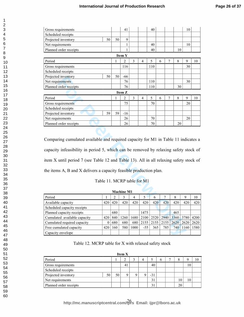
Gross requirements 41 40 10

Scheduled receipts

Projected inventory 50 50 9



Item Y

Period 1 2 3 4 5 6 7 8 9 10


Scheduled receipts

Projected inventory 50 50 -66



Item Z

Period 1 2 3 4 5 6 7 8 9 10


Scheduled receipts

Projected inventory 59 59 -16



Comparing cumulated available and required capacity for M1 in Table 11 indicates a

capacity infeasibility in period 5, which can be removed by relaxing safety stock of

item X until period 7 (see Table 12 and Table 13). All in all relaxing safety stock of

the items A, B and X delivers a capacity feasible production plan.


Machine M1

Period 1 2 3 4 5 6 7 8 9 10


Scheduled capacity receipts




Free cumulated capacity 420 160 580 1000 -55 365 785 740 1160 1580

Capacity envelope

Table 12. MCRP table for X with relaxed safety stock

Item X

Period 1 2 3 4 5 6 7 8 9 10


Scheduled receipts

Projected inventory 50 50 9 9 9 -31



Page 26 of 37



123456789101112131415161718192021222324252627282930313233343536373839404142434445464748495051525354555657585960

For Peer Review O

nly

27

Calculated lead time 0 0 0 0 0,6 0,0 0,0 0,4 0,0 0,0


Table 13. MCRP table for M1 with relaxed safety stock

Machine M1

Period 1 2 3 4 5 6 7 8 9 10


Scheduled capacity receipts






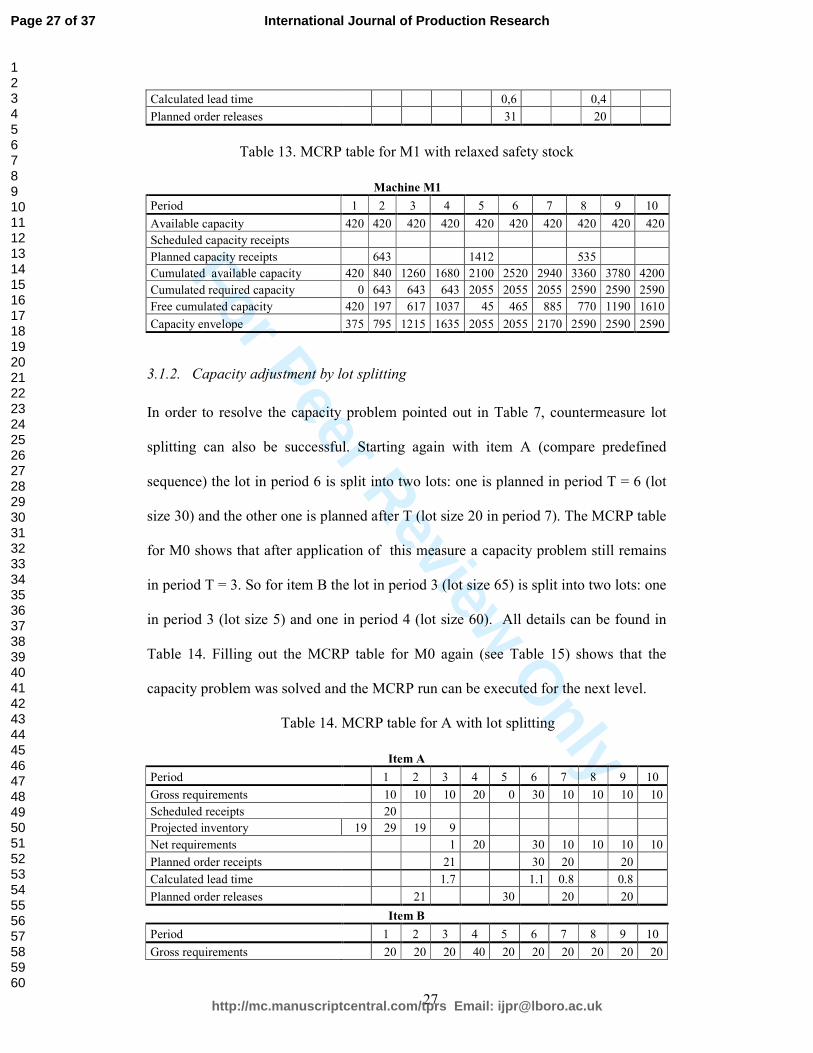
3.1.2. Capacity adjustment by lot splitting

In order to resolve the capacity problem pointed out in Table 7, countermeasure lot

splitting can also be successful. Starting again with item A (compare predefined

sequence) the lot in period 6 is split into two lots: one is planned in period T = 6 (lot

size 30) and the other one is planned after T (lot size 20 in period 7). The MCRP table

for M0 shows that after application of this measure a capacity problem still remains

in period T = 3. So for item B the lot in period 3 (lot size 65) is split into two lots: one

in period 3 (lot size 5) and one in period 4 (lot size 60). All details can be found in

Table 14. Filling out the MCRP table for M0 again (see Table 15) shows that the

capacity problem was solved and the MCRP run can be executed for the next level.

Table 14. MCRP table for A with lot splitting

Item A

Period 1 2 3 4 5 6 7 8 9 10






Calculated lead time 0 0 1.7 0,0 0,0 1.1 0.8 0,0 0.8 0,0


Item B

Period 1 2 3 4 5 6 7 8 9 10


Page 27 of 37



123456789101112131415161718192021222324252627282930313233343536373839404142434445464748495051525354555657585960

For Peer Review O

nly

28

Scheduled receipts 0 0 0 0 0 0 0 0 0 0




Calculated lead time 0 0 1.1 1.9 0,0 1.4 0,0 0,0 1.0 0,0


Table 15. MCRP table for M0 with lot splitting

Machine M0

Period 1 2 3 4 5 6 7 8 9 10


Scheduled capacity receipts 325 0 0 0 0 0 0 0 0 0

Planned capacity receipts 0 0 424 580 0 1045 325 0 725 0





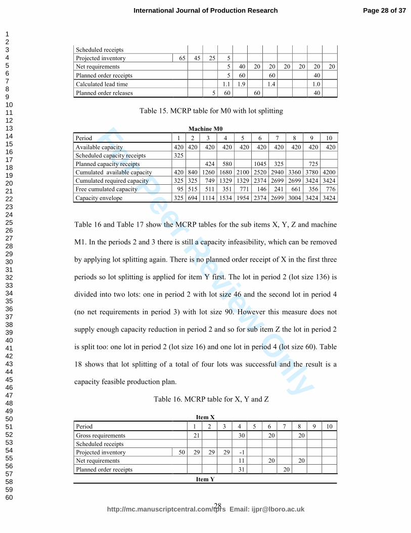
Table 16 and Table 17 show the MCRP tables for the sub items X, Y, Z and machine

M1. In the periods 2 and 3 there is still a capacity infeasibility, which can be removed

by applying lot splitting again. There is no planned order receipt of X in the first three

periods so lot splitting is applied for item Y first. The lot in period 2 (lot size 136) is

divided into two lots: one in period 2 with lot size 46 and the second lot in period 4

(no net requirements in period 3) with lot size 90. However this measure does not

supply enough capacity reduction in period 2 and so for sub item Z the lot in period 2

is split too: one lot in period 2 (lot size 16) and one lot in period 4 (lot size 60). Table

18 shows that lot splitting of a total of four lots was successful and the result is a

capacity feasible production plan.

Table 16. MCRP table for X, Y and Z

Item X

Period 1 2 3 4 5 6 7 8 9 10

Gross requirements 21

30

20

20

Scheduled receipts




Item Y

Page 28 of 37



123456789101112131415161718192021222324252627282930313233343536373839404142434445464748495051525354555657585960

For Peer Review O

nly

29

Period 1 2 3 4 5 6 7 8 9 10

Gross requirements 86 90 20 40 20

Scheduled receipts

Projected inventory 50 -36



Item Z

Period 1 2 3 4 5 6 7 8 9 10


Scheduled receipts

Projected inventory 59 -6




Machine M1

Period 1 2 3 4 5 6 7 8 9 10






Free cumulated capacity 420 -503 -83 90 375 455 705 790 1210 1630

Capacity envelope

Table 18. MCRP table for M1 with lot splitting

Machine M1

Period 1 2 3 4 5 6 7 8 9 10

Available Capacity 420 420 420 420 420 420 420 420 420 420




Cumulated required capacity 413 413 1645 1780 2120 2290 2625 2625 2625



4. Conclusion

In this paper an approach for coping with the finite capacity of machines in an MRP

procedure was developed (MCRP). An additional procedure, capacitating, was

inserted between the steps lot-sizing and offsetting to guarantee capacity feasible

production plans. To reach this result different measures for capacity adjustment have

been proposed and two of them (relaxing safety stock and lot splitting) have been

Page 29 of 37



123456789101112131415161718192021222324252627282930313233343536373839404142434445464748495051525354555657585960

For Peer Review O

nly

30

successfully applied in a detailed example. Additionally, lead times for offsetting are

calculated dynamically to take lot sizes, inventory and the required machine capacity

into account.

Some limitations of the proposed approach are the lack of stochastic influences and

the lack of a safety lead time which could be advantageous mainly to cope with

unreliability in supply (see van Kampen et al. 2010). A safety lead time can be

integrated easily by adding this time into the calculation of the dynamic lead time.

Furthermore there is no guarantee that the listed countermeasures lead to a capacity

feasible production plan. If the application of all countermeasures is not successful,

the master production schedule (MPS) has to be changed or otherwise tardiness of

some jobs has to be accepted.

On the other hand some managerial goals (e.g. increasing service level, reducing

holding costs, changeover costs or tardiness) can be influenced positively by choosing

adequate parameters. Integrating capacity planning in an MRP run can supersede or at

least reduce a time consuming revision of the schedules by the user.

In real world implementation most firms integrate traditional MRP in their ERP.

Because of the weaknesses of MRP (no capacity planning and fixed lead times) the

planners have to adapt the plans subsequently to ensure feasibility – this job list

adaption is in general a difficult and time consuming task. The suggested approach

has advantage over traditional MRP as well as MRP-CRP (Harl, 1983), MRP-SFC

(Taal and Wortmann, 1997) and FCMRP (Pandey et al., 2000). The capacity

planning is performed during the MRP-Run between lot sizing and offsetting, a load

depending lead time is calculated and therefore in more cases than in traditional MRP

capacity feasible planes are determined. Another further available development of

MRP is finite capacity scheduling algorithm (for instance Billington and Thomas,

Page 30 of 37



123456789101112131415161718192021222324252627282930313233343536373839404142434445464748495051525354555657585960

For Peer Review O

nly

31

1983; Sum and Hill, 1993; Cho and Seo, 2009) offered in Advanced Planning

Systems like Detailed Scheduling in SAP/APO. General scheduling algorithms are

not often used in industrial environments because of lack of understanding, missing

constraints for real-life problems, deviation of the deterministic model for the

stochastic real world and the long calculation times needed.

For further research material capacity requirement planning with dynamic lead

times should be implemented in simulation software to test more complex scenarios

and to compare the performance of MCRP with traditional MRP.

Page 31 of 37



123456789101112131415161718192021222324252627282930313233343536373839404142434445464748495051525354555657585960

For Peer Review O

nly

32

References

Baker, K., 1984. Sequencing rules and due-date assignments in a job shop.

Management Science, 30(9), 1093-1104.

Bakke, N. A. and Hellberg, R., 1993. The challenges of capacity planning.

International Journal of Production Economics, 30/31, 243-264.

Billington, P. J. and Thomas, L. J., 1983. Mathematical programming approaches to

capacity constraints MRP systems. Management Science, 29(10), 1126-1141.

Billington, P. J. and Thomas, L. J., 1986. Heuristics for multi-level lot-sizing with a

bottleneck. Management Science, 32(8), 1403-1415.

Chen, J. C., Fan Y.-C., Chen C.-W., 2009. Capacity requirements planning for twin

Fabs of wafer fabrication. International Journal of Production Research,

47(16), 4473-4496.

Choi, B. K. and Seo, J. C., 2009. Capacity-filtering algorithms for finite-capacity

planning of a flexible flow line. International Journal of Production Research,

47(12), 3363-3386.

Groff, G. K., 1979. A lot-sizing rule for time phased component demand. Production

and Inventory Management, 20, 47-53.

Harl, J. E., 1983. Reducing capacity problems in material requirements planning

system. Production and Inventory Management, 24(3), 52-60.

Haddock, J. and Hubicki, D. E., 1989. Which lot-sizing techniques are used in

material requirements planning? Production and Inventory Management

Journal, 30(3), 53-56.

Hopp, W. J. and Spearman, M. L., 2008. Factory Physics – Foundations of

Manufacturing Management. Chicago: Irwin.

Hübl, A., Altendorfer, K., Jodlbauer, H. and Pilstl J., 2009. Customer Driven Capacity

Setting. Advances in Production Management Systems APMS 2009

Proceedings, Bordeaux, France.

Kanet, J. J., 1983. Toward a better understanding of lead times in MRP systems.

Journal of Operations Management, 6(3), 305-315.

Kanet, J. J., Gorman, M. F. and Stößlein, M., 2010. Dynamic planned safety stocks in

supply networks. International Journal of Production Research, 48(22), 6859-

6880.

Kanet, J. J. and Stößlein, M., 2010. Integrating production planning and control:

towards a simple model for Capacitated ERP. Production Planning & Control,

21(3), 286-300.

Lee, H.-G., Park, N. and Park, J., 2009. A high performance finite capacitated MRP

process using a computational grid. International Journal of Production

Research, 47(8), 2109-2123.

Nagendra, P., Das, S. and Chao, X., 1994. Introducing capacity constraints in the

MRP algorithm. Proceedings of 1994 Japan – U.S.A. Symposium on Flexible

Automation – A Pacific Rim Conference, 213-216.

Nagendra, P. and Das, S., 2001. Finite capacity scheduling method for MRP with lot

size restrictions. International Journal of Production Research, 39(8), 1603-

1623.

Orlicky, J. A., 1975. Material Requirements Planning. New York: McGraw Hill.

Pandey, P. C., Yenradee, P. and Archariyapruek, S., 2000. A finite capacity material

requirements planning system, Production Planning & Control, 11(2), 113-

121.

Page 32 of 37



123456789101112131415161718192021222324252627282930313233343536373839404142434445464748495051525354555657585960

For Peer Review O

nly

33

Ram, B., Naghshineh-Pour, M. R. and Yu, X., 2006. Material requirements planning

with flexible bills-of-material. International Journal of Production Research,

44(2), 399-415.

Sum, C. C. and Hill, A. V., 1993. A new framework for manufacturing planning and

control systems. Decision Sciences, 24, 739-760.

Taal, M. and Wortmann, J. C., 1997. Integrating MRP and finite capacity planning.

Production Planning & Control, 8(3), 245-254.

Tardif, V., 1995. Detecting and correcting scheduling infeasibilities in a multi-level,

finite-capacity, production environment. Doctoral dissertation, Department of

Industrial Engineering and Management Sciences, Northwestern University,

Evanston, IL.

Van Kampen,T. J., van Donk, D. P. and van der Zee, D.-J., 2010. Safety stock or

safety lead time: coping with unreliability in demand and supply, International

Journal of Production Research, 48(24), 7463-7481.

Vanhoucke, M. and Debels, D., 2009. A finite-capacity production scheduling

procedure for a Belgian steel company. International Journal of Production

Research, 47(3), 561-584.

Wuttipornpun, T. and Yenradee, P., 2004. Development of finite capacity material

requirement planning system for assembly operations. Production Planning &

Control, 15(5), 534-549.

Wuttipornpun, T. and Yenradee, P., 2007. Performance of TOC based finite capacity

material requirement planning system for a multi-stage assembly factory.

Production Planning & Control, 18(8), 703-715.

Page 33 of 37



123456789101112131415161718192021222324252627282930313233343536373839404142434445464748495051525354555657585960

For Peer Review Only

Netting


Offsetting

Gross requirements Level 0

Gross requirements Level i

i=i+1 Net requirements

i=0

Planned order receipts

Planned order releases

Scheduled receipts Inventory

Complete Level i

Page 34 of 37



123456789101112131415161718192021222324252627282930313233343536373839404142434445464748495051525354555657585960


Netting


Offsetting

Gross requirements Level 0

Gross requirements Level i

i=i+1 Net requirements

i=0

Planned order receipts

Planned order releases

Scheduled receipts Inventory

Complete Level i

Capacitating

Dynamic lead time

Complete Level i

Complete Level i

Available Capacity Scheduled receipts

Page 35 of 37



123456789101112131415161718192021222324252627282930313233343536373839404142434445464748495051525354555657585960


Scheduled receipts or planned oders of levels with lower level codes

Planned order

Cumulated available capacity


Capacity envelope

e3

a3-r3

e2

e1

a1-r1

a2-r2

Page 36 of 37



123456789101112131415161718192021222324252627282930313233343536373839404142434445464748495051525354555657585960


Scheduled receipts or planned oders of levels with lower level codes

Planned order


Capacity envelope

Release dates

e3 e3-c3,1

l3,1

capSR3

capSR3

capSR3

capSR3

l3,1

Page 37 of 37



123456789101112131415161718192021222324252627282930313233343536373839404142434445464748495051525354555657585960

material and capacity requirements planning with dynamic

Documents