material qualification methodology for 2x2 biaxially
TRANSCRIPT

Advanced General Aviation Transport Experiments
Material Qualification Methodology for 2X2 Biaxially Braided RTM Composite
Material Systems AGATE-WP3.3-033048-116 October 2001 J. Tomblin, W. Seneviratne, Y. Ng National Institute for Aviation Research Wichita State University Wichita, KS 67260-0093 Ric Abbott Raytheon Aircraft Company Wichita, KS 67206-0085 Steve Stenard A&P Technology Cincinnati, OH 45245-1055
2
TABLE OF CONTENTS
ITEM PAGE 1.0 INTRODUCTION ……………………………………………………………. 3
1.1 Scope ……………………………………………………………….. 3 1.2 Field of Application ……………………………………………….. 3 1.3 Applicable Documents .……………………….……….………... 3 1.4 Abbreviations, Acronyms, and Definitions ……….…………... 4
2.0 APPLICABLE FAA REGULATIONS AND RECOMMENDATIONS....… 4
2.1 Applicable Federal Regulations…….……………………………. 5 2.2 Applicable Advisory Circular Recommendations.……………. 6
3.0 COMPOSITE TEST METHODS AND SPECIMEN GEOMETRY ……… 7
3.1 Specimen Manufacturing ………………………………………..… 8 3.2 Environmental Conditionings …………………………………… 14 3.3 Nonambient Testing ……………………………………………... 15 3.4 Specimen Geometry and Test Methods ……………………… 16
4.0 QUALIFICATION PROGRAM …………………………………………… 44
4.1 Introduction ……………………………………………………….. 44 4.2 General …………………………………………………………….. 44 4.3 Technical Requirements ………………………………………... 44 4.4 Material Qualification Program for Base Resin and Fiber … 45 4.5 Material Qualification Program for Cured Lamina Main Properties …………………………………………………… 46
5.0 DESIGN ALLOWABLE GENERATION ………………………………… 52
5.1 Introduction ……………………………………………………….. 52 5.2 Statistical Analysis ………………………………………………... 53 5.3 Material Performance Envelope and Interpolation…………... 70
APPENDIX A - Example Panel Size Requirements ……………………….. 82 APPENDIX B - Example Panel Manufacturing Procedure Using RTM .. 93 APPENDIX C - Combined Loading Compression (CLC) Proposed
Standard …………………………………………….…………102

3
1.0 INTRODUCTION The purpose of this qualification plan is to describe an acceptable program to substantiate that the materials and processes employed meet appropriate Federal Aviation Administration (FAA) requirements. These requirements apply to the original material qualification. Once certified, changes to the material, process, tooling and/or facility require a review and it may be required that some (or all) of these tests be repeated. 1.1 Scope
This plan gives specific information about the qualification program for a 2x2 biaxially braided composite material system that is manufactured using a Resin Transfer Molding (RTM) process. Specifically, this plan covers one-part resin systems which are premixed at the resin manufacturer and combined with a braided sock preform via a RTM process.
1.2 Field of Application
The qualification plan describes material qualification methodology for a 2x2 biaxially braided composite material system that is manufactured using a resin transfer molding (RTM) process. Additionally, this plan establishes testing methods and process controls necessary to certify composite materials used for airframe components under FAR Part 23 requirements. In some cases, unique characteristics of a material system or its application may require testing beyond that described in this document. In these situations, Aircraft Certification Offices (ACOs) may require additional testing to demonstrate compliance to the applicable Federal Aviation Regulations (FARs).
1.3 Applicable Documents
MIL-HDBK-17-1E,2D,3E - Military Handbook for Polymer Matrix Composites
SAE AMS 2980/0-5 - Technical Specification : Carbon Fiber Fabric Epoxy Resin Wet Lay-up Repair
FAA Code of Federal Regulations (CFR) 14 : Aeronautics and Space FAA Advisory Circular 20-107A : Composite Aircraft Structures
FAA Advisory Circular 21-26: Quality Control for the Manufacture of Composite Materials

4
1.4 Abbreviations, Acronyms and Definitions
ACO Aircraft Certification Office AMS Aerospace Material Specification
ANOVA analysis of variance ASTM American Society for Testing and Materials
CPT cured ply thickness CTD cold temperature dry DAR Designated Airworthiness Representative DMA dynamic mechanical analysis DSC differential scanning calorimetry ETD elevated temperature dry ETW elevated temperature wet FAA Federal Aviation Administration FAR Federal Aviation Regulations
FAW fiber areal weight FTIR Fourier transform infrared spectroscopy
FV fiber volume fraction HPLC high performance liquid chromatography MIDO Manufacturing Inspection District Office
MRB material review board NDI nondestructive inspection
NIST National Institute of Standards and Technology OEM Original Equipment Manufacturer QA quality assurance QC quality control RTD room temperature dry RTM resin transfer molding SACMA Suppliers of Advanced Composite Materials Association SAE Society of Automotive Engineers Tg glass transition temperature TOD Threshold of Detectibility A-Basis 95% lower confidence limit on the first population percentile B-Basis 95% lower confidence limit on the tenth population percentile

5
2.0 APPLICABLE FAA REGULATIONS AND RECOMMENDATIONS This qualification plan was developed as a means to show compliance with FAR Part 23 requirements. Specifically, this document provides material qualification methodology to show compliance with the following FAR Part 23 paragraphs: 2.1 Applicable Federal Regulations
FAR 23.601 General.
The suitability of each questionable design detail and part having an important bearing on safety in operations must be established by tests. FAR 23.603 Materials and Workmanship (a) The suitability and durability of materials used for parts, the failure
of which could adversely affect safety, must -
(1) Be established by experience or tests; (2) Meet approved specifications that ensure their having the
strength and other properties assumed in the design data; and
(3) Take into account the effects of environmental conditions such as temperature and humidity, expected in service.
(b) Workmanship must be of a high standard.
FAR 23.605 Fabrication Methods
(a) The methods of fabrication used must produce consistently sound structures. If a fabrication process (such as gluing, spot welding, or heat-treating) requires close control to reach this objective, the process must be performed under an approved process specification.
(b) Each new aircraft fabrication method must be substantiated by a
test program.
FAR 23.613 Material Strength Properties and Design Values

6
(a) Material strength properties must be based on enough tests of
material meeting specifications to establish design values on a statistical basis.
(b) Design values must be chosen to minimize the probability of
structural failure due to material variability. Except as provided in paragraph (e) of this section, compliance with this paragraph must be shown by selecting design values that ensure material strength with the following probability:
(1) Where applied loads are eventually distributed through a
single member within an assembly, the failure of which would result in loss of structural integrity of the component; 99 percent probability with 95 percent confidence.
(2) For redundant structure, in which the failure of individual
elements would result in applied loads being safely distributed to other load carrying members; 90 percent probability with 95 percent confidence.
(c) The effects of temperature on allowable stresses used for design in
an essential component or structure must be considered where thermal effects are significant under normal operating conditions.
(d) The design of the structure must minimize the probability of
catastrophic fatigue failure, particularly at points of stress concentration.
(e) Design values greater than the guaranteed minimums required by
this section may be used where only guaranteed minimum values are normally allowed if a "premium selection" of the material is made in which a specimen of each individual item is tested before use to determine that the actual strength properties of that particular item will equal or exceed those used in design.
2.2 Applicable Advisory Circular Recommendations The following FAA advisory circulars present recommendations for
showing compliance with FAA regulations associated with composite materials. These circulars are considered essential in certification process for composite aircraft components as well as for establishing quality control provisions for material receiving and manufacturing.
7
2.2.1 AC 20-107A - Composite Aircraft Structures
This advisory circular sets forth an acceptable, but not the only, means of showing compliance with the provisions of Federal Aviation Regulation (FAR), Parts 23, 25, 27, and 29 regarding airworthiness type certification requirements for composite aircraft structures, involving fiber reinforced materials, e.g., carbon (graphite), boron, aramid (Kevlar), and glass reinforced plastics. Guidance information is also presented on associated quality control and repair aspects.
2.2.2 AC21-26 – Quality Control for the Manufacture of Composite Structures
This advisory circular (AC) provides information and guidance concerning an acceptable means, but not the only means, of demonstrating compliance with the requirements of Federal Aviation Regulations (FAR) Part 21, Certification Procedures for Products and Parts, regarding quality control (QC) systems for the manufacture of composite structures involving fiber reinforced materials, e.g., carbon (graphite), boron, aramid (Kevlar), and glass reinforced polymeric materials. This AC also provides guidance regarding the essential features of QC systems for composites as mentioned in AC 20-107, Composite Aircraft Structure. Consideration will be given to any other method of compliance the applicant elects to present to the Federal Aviation Administration (FAA).
3.0 COMPOSITE TEST METHODS AND SPECIMEN GEOMETRY This section specifies the composite test procedures, specimen manufacturing procedures, panel size requirements, environmental conditioning and specimen geometry to be used in a typical material qualification by referring to existing standards. Drawings for each specimen’s geometry are provided with dimensions and tolerances for conformity purposes. Any specific additions or changes to the referenced test standard were also summarized. Although SAE AMS 2980/0-5 applies to field repair wet-layup systems, the general format of the qualification program has been adopted for this document. All specimens shall be fabricated according to the appropriate process specification to the geometry defined in this section and FAA conformity established by an FAA Manufacturing Inspection District Office (MIDO) employee or the FAA may delegate this to a Designated Airworthiness Representative (DAR). For the purposes of material properties qualification, each of the following paragraphs, serves as the engineering definition of the specimen in the same way as would a drawing.
8
3.1 Specimen Manufacturing
Detailed guidelines for manufacturing test panels for qualification testing are given in Appendix B specific to the RTM process.
3.1.1 Number of Specimens
The number of specimens required for qualification is dependent on the purpose for the material system. If a redundant load path exists within the design, a B-basis number may be used to substantiate the design allowable. If a single load path exists, an A-basis number may be required. Section 4 describes the specific number of tests required for each environmental test condition.
3.1.2 Panel Sizes and Quantity Requirement
Appendix A lists the required panel sizes for each test method as well as the anticipated number of specimens for each batch of material for both axial and transverse directions. Requirements for a statistically significant design allowable require three unique batches of material (see Section 4.5.1) with a total of six specimens per loading condition of each batch.
3.1.3 Panel Manufacturing
Appendix B details a manufacturing procedure, which may be used to produce the panels for the specimens required for qualification. Specific consumable items, such as release agent, may be substituted depending on the specific mold material and resin. A step-by-step RTM setup card must be prepared listing each step throughout the process (see Appendix B) for each panel. Panel ID along with the resin and fiber batch/lot ID’s must be included in this sheet. Operators MUST initial each step after performing the corresponding task. Any deviation from the card MUST be documented in the panel inspection sheet attached to the end of the RTM setup card. Mold temperature may be monitored and/or recorded throughout the cure cycle.

9
3.1.4 Batch Variability
Batch variability for B-basis requirements is obtained by combining resin and fiber batches during RTM as shown in Table 3.1.
Table 3.1 Batch Variability for B-basis batch requirements.
Resin (1) Resin (2)
Braid (A) Batch 1 N/A
Braid (B) Batch 2 Batch 3
As shown in Table 3.1, the batch variability depends on the fiber-resin combinations. For B-basis allowables two unique batches of braided fibers (Braid A and Braid B) and two unique batches of one-part resin systems (Resin 1 and Resin 2) are required. If the resin is a two-part system, Resin 1 and Resin 2 must be combinations of two unique sets of part A and part B as shown in Figure 3.1.
Figure 3.1 Batch variability for two-part resin systems.
Part A (1)
Resin (1)
Part B (1) Part A (2)
Resin (2)
Part B (2)
Braid (A) Braid (B) Braid (B)
BATCH 1 BATCH 2 BATCH 3

10
SPECIMEN SELECTION METHODOLOGY AND BATCHTRACEABILITY
PER ENVIRONMENTAL CONDITION AND TEST METHOD
MaterialBatch
PanelManufacturing& IndependentCure Process
Number ofSpecimens
Required perTest Method &Environment
BATCH 2
PANEL 4
3 spec.
PANEL 3
3 spec.
BATCH 3
PANEL 6
3 spec.
PANEL 5
3 spec.
BATCH 1
PANEL 2
3 spec.
PANEL 1
3 spec.
18 SPECIMENS TOTAL
Figure 3.2 B-basis specimen and batch traceability

11
3.1.5 Tabs
Where tabs are added to the specimen for the purpose of introducing loads, they shall be bonded to the specimen using epoxy adhesive that cures at a minimum of 100o F below the panel cure temperature. The intention of the 1000 F margin is to avoid altering the mechanical properties of the specimen. According to this rule, 3500 F cure prepreg systems may be bonded with tab material using film adhesives that cure at a maximum of 2500 F. 2500 F cure prepreg systems may be bonded with tab material using two-part epoxy paste adhesives that cure at a maximum of 1500 F. Strain compatible tabbing material should be used which commonly consists of glass or graphite woven fabric. Strain compatible tabbing material is defined as tabbing material that will yield acceptable specimen failure modes. In some cases, it is necessary to control adhesive bondline thickness to achieve acceptable specimen failure modes. Acceptable failure modes must be maintained within the specimens. The sub-panel reference edge should be used during the tabbing process to insure proper tab alignment.
3.1.6 Specimen Machining
Care should be used in cutting of sub-panels to maintain fiber orientation with respect to the reference edges as defined in section 3.1.3. To insure that this is maintained, a subpanel cut should always be based upon the original manufacturing panel reference edge. This may be accomplished by using locator pins or test indicators during cutting. The sub-panel reference edge should also be used as a reference for the sectioning of individual specimens. Precautions should be taken to insure that accumulation of fiber direction error does not exceed 0.250.
In general, specimens are sectioned from sub-panels using a water-cooled diamond saw with care taken not to overheat the specimen that may result in matrix charring. Specimens are then generally surface ground to final dimensions to achieve desired dimensional tolerances and surface finish.
All dimensional tolerances must be achieved according to the specifications provided in section 3.4 for each test method. In cases where dimensional tolerances are not met, the specimens may be reworked.

12
3.1.7 Specimen Selection
For each material or property, batch replicates should be sampled from at least two different test panels covering at least two independent processing cycles per section 3.1.3. Figures 3.2 present guidelines for specimen selection from each batch/panel. Specimens taken from each individual panel should be selected randomly. Test specimens should not be extracted from panel areas having indications of questionable quality either visually or as determined from non-destructive inspection techniques.
3.1.8 Specimen Naming
An individual specimen naming system should be devised to guarantee traceability to the original subpanel, panel, test method, test condition and batch. Evidence of traceability should be established by a FAA MIDO representative or designated DAR. Skewed lines may be drawn across each subpanel with a permanent marker or paint pen before specimen sectioning to allow subpanel or panel reconstruction after testing as shown in Figure 3.3. These may be very important when tracking outliers within the material data after testing.
Skewed Lines
Figure 3.3 Skewed lines drawn across subpanel used for reconstruction.
13
3.1.9 Strain Gage Bonding
ASTM E1237 should be used as a general guide for strain gage installation with the following certain recommendations specific to composite materials :
• Isopropyl alcohol should be used for any wet abrading or surface
cleaning. • 280 to 600 grit sandpaper should be used for abrading the surface,
taking care not to sever or expose any fibers. • If the adhesive used to bond the gage is to be post – cured, the curing
temperature must be at least 1000 F below the cure temperature of the prepreg system. This ensures that the adhesive cure cycle will not affect the mechanical properties that will be tested.
• Specimens that are humidity conditioned prior to testing should be gaged after the conditioning has taken place. Humidity aged specimens may be exposed to ambient conditions for a maximum of 2 hours for application of the gages.
• If soldering lead wiring, care must be taken not to burn the matrix of the test coupon.
• If possible, gage sizes should be selected such that the gage area is greater than three times the repetitive pattern of the braid. This may not be possible with some test methods; however, the gage area should be greater than a single repetitive pattern of the braid.
3.1.10 Specimen Dimensioning and Inspection
All dimensions to be used in the calculations of mechanical and physical properties should be recorded as specified in the respective figures. These dimensions must meet the dimensional requirements in appropriate drawing figures. All thickness measurements should be made with point or ball micrometers and all width measurements with calipers. The accuracy of all measuring instruments should be traceable to the National Institute for Standards and Technology (NIST). In the case of tabbed specimens, all measurements should be taken after the bonding of tabs and final specimen machining. For humidity aged specimens, all dimensioning should be recorded prior to environmental conditioning process. A minimum of one randomly selected specimen from each subpanel must be inspected for every dimensional requirement stated in appropriate figure. If the randomly selected specimen fails any one of the requirements, every specimen must be inspected for that dimensional requirement. The specimens that do not meet any dimensional requirement must be reinspected after rework has been accomplished. FAA Form 8130-9 must be used to indicate any deviation to FAA approved test plan.
14
3.2 Environmental Conditioning
Humidity aged specimens typically use accelerated conditioning to simulate the long-term exposure to humid air and establish a moisture saturation of the material. Accelerated conditioning of the specimens at 85 ± 5% relative humidity and 145 ± 5 oF will be used until moisture equilibrium is achieved. The environmental conditioning chamber must be calibrated using standards having traceability to the NIST or which have been derived from acceptable values of natural physical constants or through the use of the ratio method of self calibration techniques. ASTM D5229 and SACMA SRM 11 provide general guidelines regarding environmental conditioning and moisture absorption.
Specimens to be tested in the ‘dry’, as fabricated, condition should be exposed to ambient laboratory conditions until mechanical testing. Ambient laboratory conditions are defined as an ambient temperature range of 65 -75o F and a relative humidity range of 40-60%.
3.2.1 Traveler Specimens
In order to establish the effect of moisture with respect to the mechanical properties, specimens should be environmentally conditioned per section 3.2. Since the individual specimens may not be measured to determine the percentage of moisture content (due to size and tab effects), traveler coupons of (approximately 1" x 1" x specimen thickness) should be used to establish the weight gain measurements. Individual traveler specimens should be obtained from the representative panel from which the mechanical test specimens were obtained. One traveler specimen per qualification panel per batch is required.
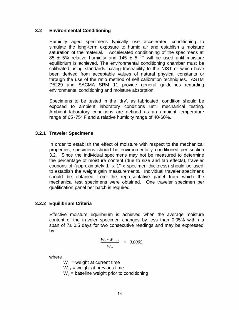
3.2.2 Equilibrium Criteria
Effective moisture equilibrium is achieved when the average moisture content of the traveler specimen changes by less than 0.05% within a span of 7± 0.5 days for two consecutive readings and may be expressed by
where
Wi = weight at current time Wi-1 = weight at previous time Wb = baseline weight prior to conditioning
0.0005 < WW - W
b
1 - ii

15
If the traveler coupons pass the criteria for two consecutive readings, the specimens may be removed from the environmental chamber and placed in a sealed bag along with a moist paper towel for a maximum of 14 days until mechanical testing. The specimens should be at room temperature (70 ± 5o F) for at least 12 hours prior to testing. Strain gauged specimens may be removed from the controlled environment for a maximum of 2 hours for application of gages in ambient laboratory conditions as defined in section 3.2. If the moisture diffusivity constant is not required, the samples do not require drying prior to conditioning.
3.3 Nonambient Testing
In order to quantify the effect of temperature with respect to mechanical properties, increased and decreased temperature testing is required (see section 4.3). This increased and decreased temperature testing is usually accomplished using an environmental testing chamber attached to the load frame.
3.3.1 Temperature Chamber
The temperature chamber used in the environmental testing should be capable of performing all required tests with an accuracy of ± 3o F of the required temperature. The chamber must be calibrated using standards having traceability to the NIST or which have been derived from acceptable values of natural physical constants or through the use of the ratio method of self-calibration techniques. The chamber should be of adequate size that all test fixtures and load frame grips may be contained within the chamber. The chamber should also be capable of a heating rate as to reach the desired test temperature within the times specified in the following sections.
3.3.2 Testing at Elevated Temperatures
Before beginning the testing, the temperature chamber and test fixture should be pre-heated to the specified temperature. For the maximum operational temperature, the chamber and fixture should be pre-heated to a temperature of 180o F (see Section 4.3).
Each specimen should be heated to the required test temperature as verified by a thermocouple in direct contact with the specimen gage section and protected from direct exposure to the airflow. The heat up time of the specimen shall not exceed 5 minutes. The test should start
1 0 2 +
− minutes after the specimen has reached the test temperature. During

16
the test, the temperature, as measured on the specimen, shall be the required test temperature ± 5o F.
3.3.3 Testing at Sub-zero Temperatures
Before beginning the testing, the temperature chamber and test fixture should be pre-cooled to the specified temperature. For the maximum sub-zero environment, the chamber and fixture should be pre-cooled to a temperature of -65o F (see Section 4.3).
Each specimen should be cooled to the required test temperature as verified by a thermocouple in direct contact with the specimen gage section. The test should start 1
0 5 +− minutes after the specimen has
reached the test temperature. During the test, the temperature, as measured on the specimen, shall be the required test temperature ± 5o F.
3.4 Specimen Geometry and Test Methods
Testing of braided composites materials encounter difficulties due to the development of inhomogeneous local displacement fields. Therefore, the standardized test methods for conventional tape laminates may not directly applicable to braided composites.
3.4.1 General
The test methods and specimen geometry presented in the following sections refer to the actual qualification procedures and test methods used to establish design allowables for a given RTM braided material system. The following referenced publications serve as the basis for this qualification plan. The applicable issue of the standard or recommendation at the time of publication of this qualification plan should be used. In the event a revision of the testing standard or recommendation occurs during the material qualification, the extent to which it affects this qualification plan should be investigated.
The test methods described in the following sections are intended to provide basic composite properties essential to most methods of analysis. These properties are considered to provide the initial base of the “building block” approach. Additional coupon level tests and subelement tests may be required to fully substantiate the full-scale design.

17
3.4.2 References 3.4.2.1 ASTM Standards
D3039-95 Tensile Properties of Polymer Matrix Composite Materials
D5379-93 Shear Properties of Composite Materials by the V-Notched Beam Method
D2344-89 Apparent Interlaminar Shear Strength of Parallel Fiber Composites by Short-Beam Method
D792-91 Density and Specific Gravity (Relative Density) of Plastics by Displacement
D2584-94 Ignition Loss of Cured Reinforced Plastics D2734-94 Void Content of Reinforced Plastics D3171-90 Fiber Content of Resin – Matrix Composites by Matrix
Digestion
3.4.2.2 SACMA Publications SRM 8-94 Short Beam Shear Strength of Oriented Fiber-Resin
Composites SRM 18-94 Glass Transition Temperature (Tg) Determination by
DMA of Oriented Fiber-Resin Composites
3.4.2.3 Other Documents
Combined Loading Compression (CLC) Proposed Standard (Appendix C)

18
3.4.3 Braided Material Forms
The mechanical behavior of braids hinge upon the fiber geometry. The geometry of a periodic textile can be conveniently illustrated in terms of a repeating pattern, referred as the Repeating Unit Cell or RUC (Figure 3.4).
The braid angle is the angle of the braided yarns measured relative to the axis parallel to the axis of the tube (braid direction). The braided preform is produced in a tubular shape. Usually, the diameter of the resulting braid is defined at the braid angle of ±45°. The braid angle can be changed between the tensile and compressive jam angles by stretching or compressing the braid.
When a braided layer is said to be oriented 0°, the braider yarns are not aligned with the 0° (see Figures 3.5-7). The orientation of the layer represents the direction of the braid axis.
Figure 3.4 Diamond shaped unit cell of a 2-D 2x2 biaxial braid.
Diamond Shape Unit Cell

19
3.4.3.1 The Repeating Unit Cell (RUC) of ±30° Braid
Figure 3.5 Repeating Unit Cell (RUC) of ±30° braid.
0° Direction (Braid
Direction)
+30° -30°
90° Direction
60°

20
3.4.3.2 The Repeating Unit Cell (RUC) of ±45° Braid
Figure 3.6 Repeating Unit Cell (RUC) of ±45° braid.
0° Direction
(Braid Direction)
90° Direction
-45° +45°

21
3.4.3.3 The Repeating Unit Cell (RUC) of ±60° Braid
Figure 3.7 Repeating Unit Cell (RUC) of ±60° braid.
Note that the ±60° braid RUC is a 90° rotation (in-plane) of the ±30° braid RUC. Therefore, the 90° properties of ±60° braid are equivalent to the 0° direction properties of ±30° braid and 0° properties of ±60° braid are equivalent to the 90° direction properties of ±30° braid.
0° Direction (Braid
Direction)
+60° -60°
90° Direction
30°

22
3.4.5 Mechanical Property Testing and Specimen Geometry
This section describes the specific specimen geometry used to produce each individual mechanical property. Specific dimensions and tolerances are provided for each specimen taken from the referenced test method(s) as well as requirements on the parallelism and perpendicularity. Requirements for the thickness of each specimen are provided and should be adjusted based upon the nominal cured ply thickness of the material system being qualified. Specific changes and/or additions to the referenced test methods are also presented.
For general guidelines with respect to specimen dimensions and tolerances, the following reference provides guidelines for interpreting the specimen geometry as shown for each test method and/or material type:
Dimensioning and Tolerancing, American Society of Mechanical Engineers National Standard, Engineering Drawing and Related Document Practices, ASME Y14.5M-1994.

23
3.4.5.1 Tensile Strength, Modulus and Poisson’s Ratio
ASTM D3039-95 Tensile Properties of Polymer Matrix Composite Materials
a. Specimen Geometry
a.1 ±30° Braid Angle – Strength, Modulus and Poisson’s Ratio
Figure 3.8 ±30° braid angle tension specimen.
24
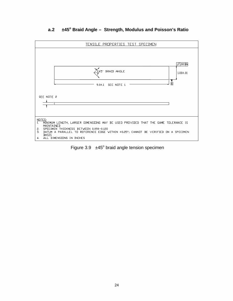
a.2 ±45o Braid Angle – Strength, Modulus and Poisson’s Ratio
Figure 3.9 ±45o braid angle tension specimen

25
a.3 ±60o Braid Angle – Strength, Modulus and Poisson’s Ratio
Figure 3.10 ±60o braid angle tension specimen
26
b. Laminate Layup and Recommended Thickness
0.150” ± 0.050” with a layup that yields a fiber volume fraction equivalent to the actual production parts.
c. Specific Additions and Changes to Referenced Test Method(s) :
c.1 Quality Control and Documentation Requirements
At least one randomly selected specimen per subpanel should be checked for all dimensional tolerances detailed on the specimen geometry figures. If the randomly selected specimen fails any one of the requirements, all specimens from that subpanel should be individually inspected for that dimension. If the specimens cannot be corrected to fall within the required tolerances, the impact of such deviation(s) must be investigated. Specimens with deviation(s) that will affect the test results must be discarded. Specimens with deviation(s) that will not affect the test results may be used provided that such deviations are documented on FAA Form 8130-9. A minimum of two width and thickness measurements must be recorded within the gage section of the specimen. The average width and thickness should be used for the final material property calculations.
c.2 Strain Gage
Perform strain gage application per section 3.1.9 as required per section 4 of this qualification plan. Upon testing system alignment verification, back-to-back strain gages are not required to verify percent bending.
c.3 Specimen Sampling
Specimen sampling should be selected randomly based upon the panel requirements delineated in Appendix A.
c.4 Recommended calculation of modulus of elasticity and
Poisson’s ratio Calculate the slope of a linear curve fit of the applicable data between the strain range given in Table 3 of ASTM D3039-95.
c.5 Environmental Conditioning
Perform specimen conditioning as outlined in section 3.2.

27
3.4.5.2 Compressive Strength and Modulus Combined Loading Compression (CLC) (see Appendix C for proposed standard)
a. Specimen Geometry
a.1 ±30o Braid Angle Compressive Strength and Modulus
Figure 3.11 ±30° braid angle compression strength and modulus
28
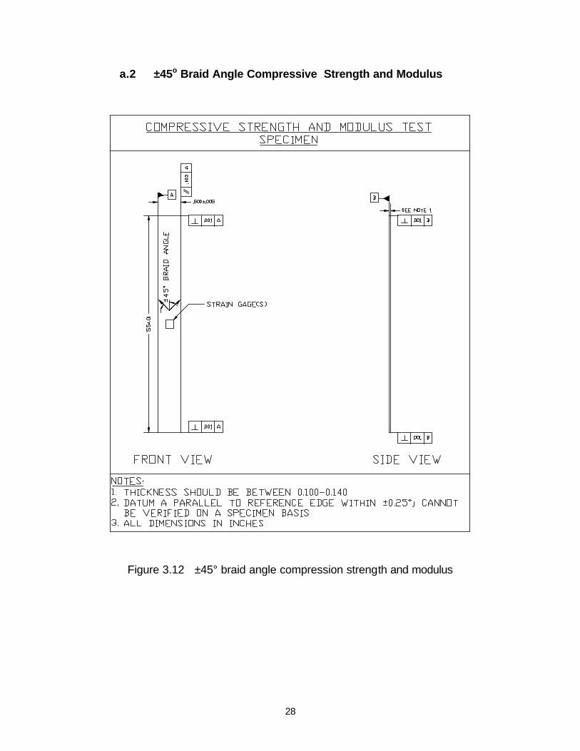
a.2 ±45o Braid Angle Compressive Strength and Modulus
Figure 3.12 ±45° braid angle compression strength and modulus

29
a.3 ±60o Braid Angle Compressive Strength and Modulus
Figure 3.13 ±60° braid angle compression strength and modulus

30
b. Laminate Layup and Recommended Thickness
0.150” ± 0.050” with a layup that yields a fiber volume fraction equivalent to the actual production parts.
c. Specific Additions and Changes to Reference Test Method(s): c1. Quality Control and Documentation Requirements
Due to the extreme sensitivity of this test method, all must be checked for all dimensional tolerances detailed on the specimen geometry figures. Particular attention should be addressed to parallelism and perpendicularity. At least one randomly selected specimen per subpanel must be checked for all dimensional tolerances on the specimen geometry. If the randomly selected specimen fails any one of the requirements, all specimens from that subpanel must be individually inspected for that dimension. If the specimens cannot be corrected to fall within the required tolerances, the impact of such deviation(s) must be investigated. Specimens with deviation(s) that will affect the test results must be discarded. Specimens with deviation(s) that will not affect the test results may be used provided that such deviations are documented on FAA Form 8130-9. A minimum of one width and thickness measurements must be recorded within the gage section of the specimen. The average width and thickness must be used for the final material property calculations.
c.2 Strain Gage
Perform strain gage application per section 3.1.9 as required per section 4 of this qualification plan. Back-to-back strain gages are not mandatory for modulus tests.
c.3 Sampling
Specimen sampling should be randomly selected based upon the panel requirements delineated in Appendix A.
c.4 Recommended calculation of modulus of elasticity
Calculate the slope of a linear curve fit of the applicable data between the 1000 – 3000 µε range as needed.
c.5 Environmental Conditioning
Perform specimen conditioning as outlined in section 3.2.

31
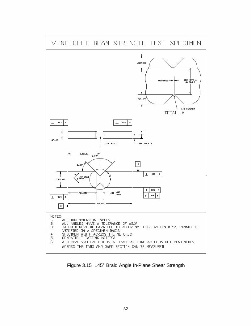
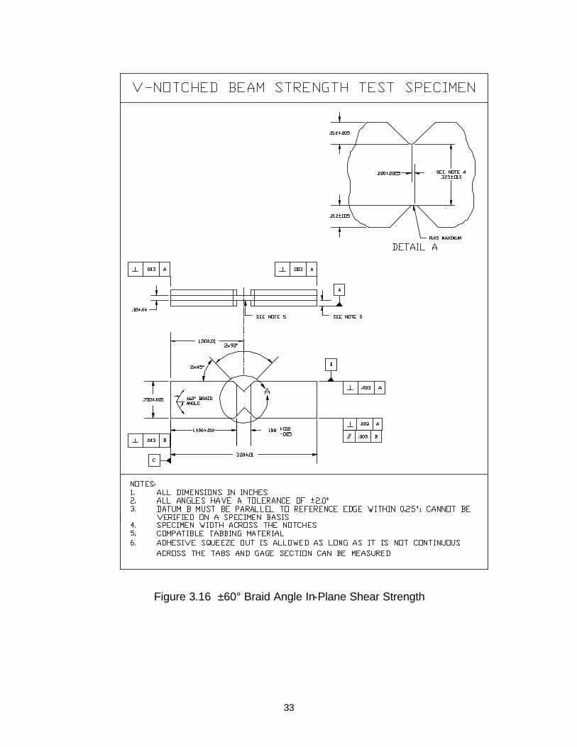
3.4.5.3 In-Plane Shear Strength and Modulus
ASTM D5379-93 Shear Properties of Composite Materials by the V-Notched Beam Method (Modified)
a. Specimen Geometry
a.1 In-Plane Shear Strength
Figure 3.14 ±30° Braid Angle In-Plane Shear Strength
32
Figure 3.15 ±45° Braid Angle In-Plane Shear Strength
33
Figure 3.16 ±60° Braid Angle In-Plane Shear Strength

34
a.2 In-Plane Shear Modulus
Figure 3.17 ±30° Braid Angle In-Plane Shear Modulus

35
Figure 3.18 ±45° Braid Angle In-Plane Shear Modulus

36
Figure 3.19 ±60° Braid Angle In-Plane Shear Modulus

37
b. Laminate Layup and Recommended Thickness 0.150” ± 0.050” with a layup that yields a fiber volume fraction equivalent to the actual production parts.
c. Specific Additions and Changes to Referenced Test Method(s) :
c.1 Quality Control and Documentation Requirements
At least one randomly selected specimen per subpanel should be checked for all dimensional tolerances detailed on the specimen geometry figures. If the randomly selected specimen fails any one of the requirements, all specimens from that subpanel must be individually inspected for that dimension. If the specimens cannot be corrected to fall within the required tolerances, the impact of such deviation(s) must be investigated. Specimens with deviation(s) that will affect the test results must be discarded. Specimens with deviation(s) that will not affect the test results may be used provided that such deviations are indicated in Form 8130-9. A minimum of one width measurement across the notches (see Figure 3.14 and 3.19, DETAIL A, NOTE 4) and two thickness measurements should be recorded within the gage section of the specimen. The average of these measurements should be used in the final material property calculations.
c.2 Strain Gage
Perform strain gage application per section 3.1.9 as required per section 4 of this qualification plan. Back-to-back strain gages are not mandatory for modulus tests if specimen thickness is adequate to prevent twisting of the specimen during testing. Sample specimens should be verified prior to beginning test plan to be twist-free.
c.3 Sampling
Specimen sampling should be randomly selected based upon the panel requirements delineated in Appendix A.
c.4 Recommended calculation of shear modulus
Calculate the slope of a linear curve fit of the applicable data between the strain range outlined on Table 1 of ASTM D5379-93.
38
c.5 Environmental Conditioning Perform specimen conditioning as outlined in section 3.2.
c.6 Tabs Tab surfaces may be ground flat after tab bonding operations if there is evidence of nonparallel tab surfaces that will cause the specimens to buckle prematurely.
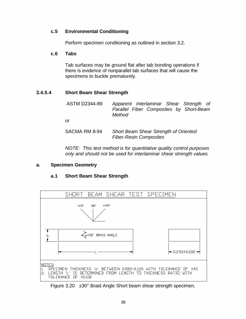
3.4.5.4 Short Beam Shear Strength
ASTM D2344-89 Apparent Interlaminar Shear Strength of Parallel Fiber Composites by Short-Beam Method
or
SACMA RM 8-94 Short Beam Shear Strength of Oriented Fiber-Resin Composites
NOTE: This test method is for quantitative quality control purposes only and should not be used for interlaminar shear strength values
a. Specimen Geometry
a.1 Short Beam Shear Strength
Figure 3.20 ±30° Braid Angle Short beam shear strength specimen.

39
Figure 3.21 ±45° Braid Angle Short beam shear strength specimen.
Figure 3.22 ±60° Braid Angle Short beam shear strength specimen.

40
b. Laminate Layup and Recommended Thickness
0.150” ± 0.050” with a layup that yields a fiber volume fraction equivalent to the actual production parts.
c. Specific Additions and Changes :
c.1 Quality Control and Documentation Requirements
At least one randomly selected specimen per subpanel should be checked for all dimensional tolerances detailed on the specimen geometry figures. If the randomly selected specimen fails any one of the requirements, all specimens from that subpanel must be individually inspected for that dimension. If the specimens cannot be corrected to fall within the required tolerances, the impact of such deviation(s) must be investigated. Specimens with deviation(s) that will affect the test results must be discarded. Specimens with deviation(s) that will not affect the test results may be used provided that such deviations are indicated in Form 8130-9. A minimum of one width and thickness measurements must be recorded. These measurements must be taken at the center of the specimen. The average of these measurements must be used in the final material property calculations.
c.2 Sampling
Specimens used for this test method are not required to follow the processing requirements delineated in section 3.1.3. Specimen sampling should be random selected based upon the requirements delineated in Appendix A.
c.3 Span and Specimen Length
Recommendations for support span and specimen lengths are delineated in Table 1 of D2344-89. However, these recommendations may be adjusted (and reported) to ensure proper failure modes.
Guidelines for the length are taken from ASTM D2344-89 in terms of the length-to-thickness ratio. For glass fibers, the length-to-thickness ratio should be 7 and for graphite fibers, the length-to-thickness ratio should be 6. The span may be adjusted to obtain proper failure modes.

41
3.4.6 Additional Test Methods 3.4.6.1 Fiber Volume Fraction 3.4.6.1.1 Fiberglass Laminates a. Procedure
ASTM D2584-94 Ignition Loss of Cured Reinforced Resins b. Specific Additions or Changes:
b.1 One sample should be tested per panel used for fabricating mechanical test coupons.
b.2 Specimens should be desiccated or oven-dried prior to taking initial weight measurement, instead of being exposed to the standard laboratory atmosphere.
3.4.6.1.2 Carbon or Graphite Laminates a. Procedure
ASTM D3171-90 Fiber Content of Resin – Matrix Composites by Matrix Digestion, Procedure B
b. Specific Additions or Changes:
b.1 One sample should be tested per panel used for fabricating mechanical test coupons.
b.2 Specimens should be desiccated or oven-dried prior to taking initial weight measurement, instead of being exposed to the standard laboratory atmosphere.
b.3 Procedure B is recommended due to the ease of process. Although procedures A and C are recommended for epoxy matrices, both require a high capital investment in equipment. Assessment as to the degree of digestion by the proposed method should be investigated prior to beginning test program for each matrix system.

42
3.4.6.2 Void Volume Fraction 3.4.6.2.1 Specimen Density a. Procedure
ASTM D792-91 Density and Specific Gravity (Relative Density) of Plastics by Displacement, Procedure A
b. Specific Additions or Changes:
b.1 One sample should be tested per panel used for fabricating mechanical test coupons.
b.2 Optimum results will be generated if samples tested for density are the same as those utilized for fiber volume fraction tests (Section 3.4.6.1).
b.3 Specimens should be desiccated or oven-dried prior to taking initial weight measurement, instead of being exposed to the standard laboratory atmosphere.
b.4 Upon immersing the specimens in water, the weight should be recorded immediately as the composite specimen will begin to absorb small amounts of water. If bubbles adhere to the sample, they should be removed immediately and the weight recorded soon thereafter.
3.4.6.2.2 Specimen Void Content a. Procedure
ASTM D2734-94 Void Content of Reinforced Plastics, Procedure A b. Specific Additions or Changes:
b.1 Although the test standard references only D2584-94, the void calculation is equally applicable to method D3171-90.
b.2 In order to avoid negative void content results, section 7.1 of D2734-94 should be strictly followed. Certified resin density measurements should be supplied from the material supplier, or procedure D792-91 should be used on a representative sample of cured neat resin in order to obtain the resin density value that is used in the void calculation.

43
3.4.6.3 Glass Transition Temperature a. Procedure
SACMA RM 18-94 Glass Transition Temperature (Tg) Determination by DMA of Oriented Fiber-Resin Composites
b. Specific Additions or Changes:
b.1 Fixture Type : Three-point bend b.2 Testing Frequency : 1 Hz b.3 Heating Rate : 5 ± 0.20 C per minute
b.4 Temperature range : test should begin from room temperature and
end at a temperature 50o C above Tg but below decomposition temperature.
b.5 Tg is determined from a logarithmic plot of the storage modulus as
a function of temperature. The Tg is determined to be the intersection of the two slopes from the storage modulus. Figure 3.23 depicts a typical plot and the Tg measurement.
Figure 3.23 Glass transition temperature determination from storage modulus.

44
4.0 Qualification Program 4.1 Introduction
This section outlines the specific number of tests required at each condition to substantiate a statistically-based design allowable for each material property. Unless noted, the following test procedures will be performed for each individual material system being qualified.
4.2 General
For a composite material system design allowable, several batches of material must be characterized to establish the statistically-based material property for each of the material systems. The definition of a batch of material for this qualification plan refers to a quantity of homogenous resin (base resin and curing agent) prepared in one operation with traceability to individual component batches as defined by the resin manufacturer. For this qualification plan, three batches of material will be required to establish a design allowable. In order to account for processing and panel-to-panel variability, the material system being qualified must also be representative of multiple processing cycles as delineated in section 3.1.3. For this qualification plan, each batch of material must be represented by a minimum of two independent processing/curing cycles.
4.3 Technical Requirements
In order to substantiate the environmental effects with respect to the material properties, several environmental conditions will be defined to represent extreme cases of exposure. The conditions defined as extreme cases in this qualification plan are listed as follows:
Cold Temperature Dry (CTD) - 65o F with an “as fabricated”
moisture content Room Temperature Dry (RTD) ambient laboratory conditions with
an “as fabricated” moisture content Elevated Temperature Dry (ETD) 180o F with an “as fabricated”
moisture content Elevated Temperature Wet (ETW) 180o F with an equilibrium moisture
weight gain in an 85% relative humidity environment per section 3.2

45
4.4 Material Qualification Program for Base Resin and Fiber
Table 4.1 describes the physical tests recommended for each batch of resin received from the material vendor. These tests should be traceable to each referenced test. These test methods are for the purpose of quality control in addition to specific values used in the normalization of material data (described in section 5.2). Some of the tests must be repeated in an incoming receiving inspection. Usually this retesting provides a verification of shipping to the airframe manufacturer and to establish that an error did not occur during shipment. In general, it should be noted that most of these properties significantly influence the producibility of the material system and commonly do not influence the resulting mechanical properties.
Listed in the Table 4.1 are suggestions taken from MIL-HDBK-17-1E for the acceptable test methods to produce each property. ASTM test methods are shown. The material vendor should describe the exact test method used for each property and such methods must comply with the test methods described in Table 4.1.
These chemical and physical tests also represent the properties of the prepreg system with the fibers and resin combined. The quality control procedures of the material vendor should be reviewed to ensure that quality control programs are in place for both the raw fiber and neat resin. The material vendor should submit these quality procedures to each manufacturer and be on file as part of the original qualification as well as part of quality assurance documentation for the airframe manufacturer.

46
Table 4.1 Recommended physical and chemical property tests to be performed by material vendor.
Test Method(s) No. Test Property
ASTM SACMA
No. of Replicates per Batch
1 Resin Content D 3529, C 613, D 5300 RM 23, RM 24 3
2 Volatile Content D 3530 - - - 3
3 Gel Time D 3532 RM 19 3
4 Resin Flow D 3531 RM 22 3
5 Fiber Areal Weight D 3776 RM 23, RM 24 3
6 IR (Infrared Spectroscopy) E 1252, E 168 - - - 3
7 HPLC (High Performance Liquid Chromatography) 1
- - - RM 20 3
8 DSC (Differential Scanning Calorimetry)
E 1356 RM 25 3
Notes : 1. Section 5.5.1 and 5.5.2 of MIL-HDBK-17-1E describes detailed
procedures that will be used when extracting resin from prepregs and performing HPLC tests.
4.5 Material Qualification Program for Cured Lamina Main Properties
The required number of material batches and replicates per batch are presented in the following sections. For the purpose of presentation, the following format was adopted to represent the required number of batches and replicates per batch:
# # x where the first # represents the required number of batches and the second # represents the required number of replicates per batch. For example, “3 x 6” refers to three batches of material and six specimens per batch for a total requirement of 18 test specimens.

47
Table 4.2 shows the cured lamina physical properties required to support the maximum operational temperature limit of the material system as well as specific data to be used in the statistical design allowable generation. Typically, the maximum operational limit for the material should have a margin that is at least 50o F below the wet glass transition temperature.
Fiber, resin and void fraction specimens are taken from each subpanel used for qualification to verify quality and to establish ranges for acceptable production.
Table 4.2 Cured lamina physical property tests.
Physical Property Test Procedure No. of Replicates per Batch
Fiber Volume ASTM D3171-901 or D2584-942 See note 3 Resin Volume ASTM D3171-901 or D2584-942 See note 3 Void Content ASTM D2734-944 See note 3 Cured Neat Resin Density ASTM D792-91 See note 5
Glass Transition Temperature (dry6) SACMA RM 18-94 3
Glass Transition Temperature (wet7) SACMA RM 18-94 3
Notes : 1 Test method used for carbon or graphite materials. 2 Test method used for fiberglass materials. 3 At least one test shall be performed on each panel manufactured for
qualification (see Appendix A and B). 4 Test method may also be applied to carbon or graphite materials. 5 Data should be provided by material supplier for each batch of material. 6 Dry specimens are “as fabricated” specimens that have been maintained
at ambient conditions in an environmentally controlled laboratory. 7 Wet specimens are humidity aged until an equilibrium moisture weight
gain is achieved per section 3.2.

48
4.5.1 ±30o Braid Qualification Requirements
Table 4.3 describes the number of tests required for each environmental condition along with the relevant test method to produce a design allowable corresponding to the 0° direction (braid direction). The format shown in each matrix is described in section 4.5. The temperature for each environmental condition is described in section 4.3.
Table 4.3 ±30o Braid qualification requirements for cured lamina main properties.
NO. OF SPECIMENS PER TEST CONDITION
FIGURE NO.
TEST
METHOD (REF.)
CTD1
RTD2
ETW3
ETD4
3.8
0o Tensile Strength
ASTM D3039-95 1x4
3x4
3x4
1x4
3.8*
0o Tensile Modulus, Strength and Poisson’s Ratio
ASTM D3039-95
1x2
3x2
3x2
1x2
3.11
0o Compressive Strength
Combined Loading Compression
1x4
3x4
3x4
1x4
3.11*
0o Compressive Strength & Modulus
Combined Loading Compression
1x2
3x2
3x2 1x2
3.14
In-Plane Shear Strength ASTM D5379-93**
1x4
3x4
3x4
1x4
3.17*
In-Plane Shear Modulus and Strength
ASTM D5379-93**
1x2
3x2
3x2 1x2
3.20
Short Beam Shear
ASTM D2344-89 --
3x6 -- --
* strain gages used during testing
** WSU modified in-plane shear test as per recommendations in ASTM D5379-93 Notes :
1 Only one batch of material is required (test temperature = -65 ± 5o F, moisture content = as fabricated5)
2 Three batches of material are required (test temperature = 70 ± 10o F, moisture content = as fabricated5)
3 Three batches of material are required (test temperature = 180 ± 5o F, moisture content = per section 3.2)
4 Only one batch of material is required (test temperature = 180 ± 5o F, moisture content = as fabricated5)
5 Dry specimens are “as fabricated” specimens that have been maintained at ambient conditions in an environmentally controlled laboratory.

49
4.5.2 ±45o Qualification Requirements
Table 4.4 describes the number of tests required for each environmental condition along with the relevant test method to produce a design allowable corresponding to the 0° direction (braid direction). For the 45o braid orientation, 0o and 90o directions are the equivalent. The format shown in each matrix is described in section 4.5. The temperature for each environmental condition is described in section 4.3.
Table 4.4 ±45° braid qualification requirements for cured lamina main properties.
NO. OF SPECIMENS PER
TEST CONDITION
FIGURE NO.
TEST
METHOD (REF.)
CTD1
RTD2
ETW3
ETD4
3.9
0o Tensile Strength
ASTM D3039-95 1x4
3x4
3x4
1x4
3.9*
0o Tensile Modulus, Strength and Poisson’s Ratio
ASTM D3039-95
1x2
3x2
3x2
1x2
3.12
0o Compressive Strength Combined Loading
Compression
1x4
3x4
3x4
1x4
3.12*
0o Compressive Strength & Modulus
Combined Loading Compression
1x2
3x2
3x2 1x2
3.15
In-Plane Shear Strength ASTM D5379-93**
1x4
3x4
3x4
1x4
3.18*
In-Plane Shear Modulus and Strength
ASTM D5379-93**
1x2
3x2
3x2 1x2
3.21
Short Beam Shear
ASTM D2344-89 --
3x6 -- --
* strain gages used during testing ** WSU modified in-plane shear test as per recommendations in ASTM
D5379-93 Notes : 1 Only one batch of material is required (test temperature = -65 ± 5o F, moisture content =
as fabricated5) 2 Three batches of material are required (test temperature = 70 ± 10o F, moisture content =
as fabricated5) 3 Three batches of material are required (test temperature = 180 ± 5o F, moisture content =
per section 3.2) 4 Only one batch of material is required (test temperature = 180 ± 5o F, moisture content =
as fabricated5) 5 Dry specimens are “as fabricated” specimens that have been maintained at ambient
conditions in an environmentally controlled laboratory.

50
4.5.3 ±60o Braid Qualification Requirements
Table 4.5 describes the number of tests required for each environmental condition along with the relevant test method to produce a design allowable corresponding to the 0° direction (braid direction). The format shown in each matrix is described in section 4.5. The temperature for each environmental condition is described in section 4.3.
Table 4.5 ±60o Braid qualification requirements for cured lamina main properties.
NO. OF SPECIMENS PER TEST CONDITION
FIGURE NO.
TEST
METHOD (REF.)
CTD1
RTD2
ETW3
ETD4
3.10
0o Tensile Strength
ASTM D3039-95 1x4
3x4
3x4
1x4
3.10*
0o Tensile Modulus, Strength and Poisson’s Ratio
ASTM D3039-95
1x2
3x2
3x2
1x2
3.13
0o Compressive Strength Combined Loading
Compression
1x4
3x4
3x4
1x4
3.13*
0o Compressive Strength & Modulus
Combined Loading Compression
1x2
3x2
3x2 1x2
3.16
In-Plane Shear Strength ASTM D5379-93**
1x4
3x4
3x4
1x4
3.19*
In-Plane Shear Modulus and Strength
ASTM D5379-93**
1x2
3x2
3x2 1x2
3.22
Short Beam Shear
ASTM D2344-89 --
3x6 -- --
* strain gages used during testing ** WSU modified in-plane shear test as per recommendations in ASTM
D5379-93 Notes : 1 Only one batch of material is required (test temperature = -65 ± 5o F, moisture content =
as fabricated5) 2 Three batches of material are required (test temperature = 70 ± 10o F, moisture content =
as fabricated5) 3 Three batches of material are required (test temperature = 180 ± 5o F, moisture content =
per section 3.2) 4 Only one batch of material is required (test temperature = 180 ± 5o F, moisture content =
as fabricated5) 5 Dry specimens are “as fabricated” specimens that have been maintained at ambient
conditions in an environmentally controlled laboratory.

51
4.5.4 Fluid Sensitivity Screening
Although epoxy-based materials historically have not been shown to be sensitive to fluids other than water or moisture, the influence of fluids other than water or moisture on the mechanical properties should be characterized. These fluids usually fall into two exposure classifications. The first class is considered to be in contact with the material for an extended period of time and the second class is considered to be wiped on and off (or evaporate) with relatively short exposure times.
To assess the degree of sensitivity of fluids other that water or moisture, Table 4.6 shows the following fluids, which will be used in this qualification plan.
Table 4.6 Fluid types used for sensitivity studies.
Fluid Type Specification
Exposure
Classification
Jet Fuel (JP-4) MIL-T-5624 Extended Period
Hydraulic Fluid (Tri-N-butyl phosphate ester) Laboratory Grade Extended Period
Solvent (Methyl Ethyl Ketone) Laboratory Grade Wipe On and Off
To assess the influence of various fluids types, a test method sensitive to matrix degradation will be used as an indicator of fluid sensitivity and compared with to the unexposed results at both room temperature dry and elevated temperature dry conditions. If significant differences occur between these results, the material systems must be reevaluated for possible fluid degradation other than water or moisture. Table 4.7 describes the fluid sensitivity-testing matrix with respect to the fluids defined in Table 4.6.

52
Table 4.7 Material qualification program for fluid resistance.
Fluid Type Test Method
Test Temp. (o F)
Exposure1
Number of Replicates2
Jet Fuel JP-4 ASTM D53793 180 See note 4 5 Hydraulic Fluid ASTM D53793 180 See note 5 5
Solvent ASTM D53793 Ambient See note 5 5
Notes : 1 Soaking in fluid at ambient temperature (immersion). 2 Only a single batch of material is required. 3 Shear strength only. 4 Exposure duration = 500 hours ± 50 hours 5 Exposure duration = 60 to 90 minutes
5.0 DESIGN ALLOWABLE GENERATION 5.1 Introduction
Upon completion of the mechanical test program and associated data reduction, the next step in the qualification procedure is to produce statistical design allowables for each mechanical property. Due to the inherent material property variability in composite materials, this variability should be acknowledged when assigning design values to each mechanical property. Although the statistical procedures presented in the following sections account for most common types of variability, it should be noted that these procedures may not account for all sources of variability.
Design allowables are determined for each strength property using the statistical procedures outlined in the following sections. In the case of modulus and Poisson’s ratio design values, the average value of all corresponding tests for each environmental condition should be utilized.
If strain design allowables are required, simple one-dimensional linear stress-strain relationships may be used to obtain corresponding strain design values. However, it should be noted that this process should approximate tensile and compressive strain behavior relatively well but may produce extremely conservative strain values in shear due to the nonlinear behavior. A more realistic approach for shear strain design

53
allowables is to use a maximum strain value of 5% (reference MIL-HDBK-17-1E, section 5.7.6).
5.2 Statistical Analysis
When compared to metallic materials, fiber reinforced composite materials exhibit a high degree of material property variability. This variability is due to many factors, including but not limited to: raw material and prepreg manufacture, material handling, part fabrication techniques, ply stacking sequence, environmental conditions, and testing techniques. This inherent variability drives up the cost of composite testing and tends to render smaller data sets than those produced for metallic materials. This necessitates the usage of statistical techniques for determining reasonable design allowables for composites.
5.2.1 Methodology
The statistical analyses and design allowable generation for both A and B basis values may be performed using the methodology presented by Shyprykevich1. In this data reduction method, the data from all environments, batches and panels are utilized jointly to obtain statistical information about the corresponding test condition. This approach utilizes essentially small data sets to generate test condition statistics such as population variability factors and corresponding basis values for pooling of test results for a specific failure mode across all test environments. This section describes an overview of this methodology as applied to a design allowable generated using the testing procedures presented in the qualification plan. For additional information regarding this methodology or statistical analyses in general, the reader is referred to either Shyprykevich1 or MIL-HDBK-17-1E, Chapter 8.
The data reduction methodology presented in this section requires several underlying assumptions in order to generate a valid design allowable. By pooling the data sets in the analysis method, the variability across environments should be comparable and the failure modes for each environment should not significantly change. The methodology presented also uses a normal distribution to analyze the data. If the assumption of normality is not acceptable, in general the Weibull distribution produces the most conservative basis values. If the variability or failure modes significantly change or if the assumption of normality is found to be violated, the traditional methods of MIL-HDBK-17 should be utilized.
1 REFERENCE : Shyprykevich, P., “The Role of Statistical Data Reduction in the Development of Design Allowables for Composites,” Test Methods for Design Allowables for Fibrous Composites : 2 nd Volume, ASTM STP 1003, C.C. Chamis, Ed., American Society for Testing and Materials, Philadelphia, PA, 1989, pp. 111-135.

54
The methodology to produce a design allowable (based upon testing completed via section 4.5 of this document) is presented through a step-wise process which assumes that all testing data for each condition and testing environment has been reduced and is in terms of failure stress. An assumption of normality is used in the method to reduce and model the behavior. The step-wise process then proceeds to determine a basis design allowable value (A or B) as follows:
(1) Normalize all relevant fiber dominated data via the procedures presented
in MIL-HDBK-17-1E, Section 2.4.3 (which is also given in section 5.2 of this document). This normalization procedure will account for variations in the fiber volume fraction between individuals specimens, panels and/or batches of material.
(2) For a single test condition (such as 0o compression strength), collect the
data for each environment being tested. Calculate the sample mean x and sample standard deviation s for each environment via
∑=
=n
iix
nx
1
1 (15)
2
1
2 )(1
1 ∑=
−−
=n
ii xx
ns (16)
For each environment, the environmental groupings must be checked for
any outliers per section 5.3.1.1 as well as for the assumption of normality per section 5.3.1.2. In addition, the variances of each environmental grouping should be checked for equality per section 5.3.1.3. If any outliers exist within each environmental grouping, the disposition of each outlier should be investigated via the procedures given in section 5.3.1.1.1. For the check of population normality, “engineering judgement” should be applied to verify that the assumption of normality is not significantly violated. If the assumption of normality is significantly violated, other statistical models should be investigated to fit the data. As stated above, the Weibull distribution provides the most conservative basis values. If the variance of each environmental grouping is significantly different as determined by the procedure described in section 5.3.1.3, traditional statistical methods of MIL-HDBK-17 should be utilized.
(3) Normalize the data in each environment by dividing the individual strength
by the mean strength for the corresponding environment. Normalizing will result in all data being close to a magnitude of 1.0. Pool all the normalized data together from each environment into one data set.

55
(4) For the pooled, normalized data set, calculate the number of samples n, the sample mean x and sample standard deviation s via eqn. (15) and (16). For the pooled data set, check for any outliers per section 5.3.1.1 as well as a visual comparison of the best normal fit and actual data per section 5.3.1.2. If any outliers exist within the pooled data set, the disposition of each outlier should be investigated via the procedures given in section 5.3.1.1.1. For the distributional check of normality, “engineering judgement” should be applied to verify that the assumption of normality is not significantly violated. If the assumption of normality is significantly violated, the other statistical models should be investigated to fit the data. In general, the Weibull distribution provides the most conservative basis value.
(5) Calculate the one-sided B-basis and A-basis tolerance factors for the
normal distribution that is based upon the number of samples in the pooled data set n. The B-basis tolerance factor (number of standard deviations), kB may be approximated by2
+−+≈
19.3
)( ln 520.0958.0 282.1 n
nek B (17)
The A-basis tolerance factor, kA may be approximated by
+−+≈
87.3
)( ln 522.0340.1 326.2 n
nek A (18)
Both approximations are accurate to within 0.2% of the tabulated values
for n greater than or equal to 16.
(6) Calculate the normal distribution B-basis allowable for the pooled data set using the pooled mean, standard deviation and tolerance factors via the equation
skxB B−= (19)
This number should essentially be a “knockdown” factor less than 1. For the A-basis value, replace kB with the value of kA obtained in step 5.
(7) Multiply the pooled basis values obtained in step 6 by the mean strength
calculated for each environment obtained in step 2. These values then become the basis values (A and B) for each individual environmental condition.
2 For additional information regarding these tolerance factors, the reader is referred to MIL-HDBK-17-1E, Chapter 8.

56
raw test data normalized by volume fraction(if needed)
collect data groupingby test environment
calculate sample meanand standard deviationfor each environment
check for outlier inenvironmental
groupings
check normalityassumption inenvironmental
groupings
normalize each environmental grouping by the correspondingsample mean
find normalized B & A basis for pooled databased upon the number of specimens,calculated KB and KA tolerance factors
multiply each environmental mean bythe normalized B & A basis to obtain
B & A basis values at each enviroment
check for equality ofvariances among
environmentalgroupings
check for outlier innormalized pooled
data
check normalityassumption in
normalized pooled data
calculate normalized pooledsample mean and standard
deviation
Figure 5.1 Step-wise data reduction procedure for design allowable generation.

57
A flow chart depicting this step-wise procedure is shown in Figure 5.1. An example of this procedure is given in section 5.3.2.
5.2.1.1 Test for Outliers
Once the strength data is generated for each testing condition, the data should be screened for outliers since these values can have a substantial influence on the statistical analysis. This screening may be done visually using graphical plots of the data as well as the quantitative procedure outlined below which is taken from MIL-HDBK-17, section 8.3.3. The data used for in the screening should be checked for outliers in both raw grouped data (by environment) as well as the normalized pooled data set.
The Maximum Normed Residual (MNR) method, as suggested by MIL-HDBK-17, is used for detecting outliers. The MNR test declares a value to be an outlier if it has an absolute deviation from the sample mean which, when compared to the sample standard deviation, is too large to be due to chance. This method can only detect one outlier at a time from a selected group or subgroup, hence once an outlier is detected, the outlier must be dispositioned (see section 5.3.1.1.1) and the analysis rerun to check for additional outliers.
Let x1, x2, … xn denote the data values in the sample of size n, and let x and s be the sample mean and standard deviation defined previously for the normal distribution. The MNR statistic is the maximum absolute deviation, from the sample mean, divided by the sample deviation
n1,2,...,i ,
max
=−
=s
xx
iMNR i (20)
The value obtained from this equation is compared to the critical value for the sample size n taken from Table 5.1. If the calculated MNR is smaller than the critical value, then no outliers are detected in the sample. If the MNR value is greater than the critical value, the data value associated with the largest value of xx i − is declared to be an outlier. If an outlier is detected, the disposition of the outlier should be investigated via the procedure described in section 5.3.1.1.1.

58
Table 5.1 Critical values (CV).
n CV n CV n CV n CV n CV- - 41 3.047 81 3.311 121 3.448 161 3.539- - 42 3.057 82 3.315 122 3.451 162 3.5413 1.154 43 3.067 83 3.319 123 3.453 163 3.5434 1.481 44 3.076 84 3.323 124 3.456 164 3.5455 1.715 45 3.085 85 3.328 125 3.459 165 3.5476 1.887 46 3.094 86 3.332 126 3.461 166 3.5497 2.020 47 3.103 87 3.336 127 3.464 167 3.5518 2.127 48 3.112 88 3.340 128 3.466 168 3.5529 2.215 49 3.120 89 3.344 129 3.469 169 3.55410 2.290 50 3.128 90 3.348 130 3.471 170 3.55611 2.355 51 3.136 91 3.352 131 3.474 171 3.55812 2.412 52 3.144 92 3.355 132 3.476 172 3.56013 2.462 53 3.151 93 3.359 133 3.479 173 3.56114 2.507 54 3.159 94 3.363 134 3.481 174 3.56315 2.548 55 3.166 95 3.366 135 3.483 175 3.56516 2.586 56 3.173 96 3.370 136 3.486 176 3.56717 2.620 57 3.180 97 3.374 137 3.488 177 3.56818 2.652 58 3.187 98 3.377 138 3.491 178 3.57019 2.681 59 3.193 99 3.381 139 3.493 179 3.57220 2.708 60 3.200 100 3.384 140 3.495 180 3.57421 2.734 61 3.206 101 3.387 141 3.497 181 3.57522 2.758 62 3.212 102 3.391 142 3.500 182 3.57723 2.780 63 3.218 103 3.394 143 3.502 183 3.57924 2.802 64 3.224 104 3.397 144 3.504 184 3.58025 2.822 65 3.230 105 3.401 145 3.506 185 3.58226 2.841 66 3.236 106 3.404 146 3.508 186 3.58427 2.859 67 3.241 107 3.407 147 3.511 187 3.58528 2.876 68 3.247 108 3.410 148 3.513 188 3.58729 2.893 69 3.252 109 3.413 149 3.515 189 3.58830 2.908 70 3.258 110 3.416 150 3.517 190 3.59031 2.924 71 3.263 111 3.419 151 3.519 191 3.59232 2.938 72 3.268 112 3.422 152 3.521 192 3.59333 2.952 73 3.273 113 3.425 153 3.523 193 3.59534 2.965 74 3.278 114 3.428 154 3.525 194 3.56635 2.978 75 3.283 115 3.431 155 3.527 195 3.59836 2.991 76 3.288 116 3.434 156 3.529 196 3.59937 3.003 77 3.292 117 3.437 157 3.531 197 3.60138 3.014 78 3.297 118 3.440 158 3.533 198 3.60339 3.025 79 3.302 119 3.442 159 3.535 199 3.60440 3.036 80 3.306 120 3.445 160 3.537 200 3.606

59
5.2.1.1.1 Dispositioning of Outliers
The rationale for dispositioning of outliers detected in the data set is taken from MIL-HDBK-17, section 2.4.4 and is primarily based upon engineering judgement so that outliers that should be retained are not casually discarded and those that should be deleted are not retained. The rationale presented attempts to separate variability apparent in the data that does not exist from material, processing parameter or environmental variability. These types of variability should be reflected in the data set and should be represented in the finalized basis value. Variability which exists from other sources, such as inferior specimen fabrication, processing parameters which fall outside the control limits, test fixture or machine deficiencies or a number of other factors both detectable and undetectable, may produce outliers in the data set and cause an unnecessary statistical penalties in the basis value. The purpose of this section is to provide some guidance to retain or delete the detected outliers.
When an outlier is detected, the first action should be to identify the cause through physical evidence. The following list is taken from MIL-HDBK-17 to give some examples of conditions that could be used as the basis for discarding outlier data:
(1) The material was out of specification (2) One or more panel or specimen fabrication parameters were outside
the specified tolerances (3) Test specimen dimensions or orientation were outside the specified
tolerance range (4) A defect was detected in the test specimen (5) An error was made in the specimen preconditioning (or conditioning
parameters were out of specified tolerance ranges) (6) The test machine and/or test fixture was improperly set up in some
specific and identifiable manner (7) The test specimen was improperly installed in the test fixture up in
some specific and identifiable manner (8) Test parameters (speed, temperature, etc.) were outside the
specified range (9) The test specimen slipped in the grips during the test (10) The test specimen failed in a mode other than the mode under test
(loss of tabs, unintended bending, failure outside the gage section, etc.)
(11) A test was purposely run to verify conditions suspected to have produced outlier data
(12) Data were improperly normalized
60
(13) A different failure mode that is still in the gage section (most specimens failed in interlaminar shear but one failed due to fiber matrix interface)
If the search for physical causes has been completed without success, engineering judgement should be used in assessing the outlier data. This section provides some guidelines in the case in which no physical determination exists but is not meant to provide rulings when data should be retained or deleted. In most cases, if the outlier's inclusion in the data set does not significantly affect calculated basis values, the outlier should simply be retained without further consideration.
In the case of a detected outlier given the step-wise process presented in section 5.3.1, two possibilities exist with respect to the corresponding data set (either environmentally grouped or pooled data): the outlier may be “high” or the outlier may be “low”. In the case in which an outlier (high or low) is detected with respect to the environmental grouping of the data but not with respect to the pooled data as described in section 5.3.1, in general, the outlier should be retained in the analysis. In the case in which the outlier is detected with respect to the environmental grouped data AND the pooled data, engineering judgement should be used in dispositioning the outlier.
Clearly, the easiest case to examine is the case in which a “high” outlier is detected. In the case of a “high” outlier, judgement should be used to consider whether the outlier is within the range of material capability. If the outlier is clearly outside the range of the material capability, the outlier should be deleted from the data set (particularly in the case of pooled data). In the case in which the “high” outlier is within the range of material capability, the outlier should be retained.
In the case of a “low” outlier without physical evidence, in general, the data should be retained. If the “low” outlier is seen to penalize the basis value severely, the FAA aircraft certification office should be consulted to discuss deletion of the outlier and possible causes for the outlier. In this case, additional testing may be required in order to substantiate this outlier deletion.
The Original Equipment Manufacturer (OEM) must take the responsibility to take real root cause corrective action to prevent the detected occurrence from affecting future production runs (i.e., if as a result of the investigation of outliers, it is determined that the fiber sizing was out of date, the OEM must insure that the problem will not reoccur in production). This may require changes in the quality control requirements or in the material specifications.

61
5.2.1.2 Normality Check
The normality of a given set of data may be verified visually by comparing the data distribution with the best-fit normal curve and using “engineering judgement” to check the fit of the distribution. The normality of the grouped data (data from different batches for same test environment) is checked as follows: The data from different batches are grouped together and sorted in an ascending order. The probability of survival at each value of the data is
1
1at survival ofy Probabilit+
−=n
ix i (21)
where n : total number of data points i : rank of the xi data value in the sorted/ordered list
xi : data value of rank “i” in the sorted/ordered list
The mean and standard deviation for the grouped data are then computed using rudimentary statistical techniques presented previously. The mean and the standard deviation are the parameters that define the normal distribution. Using this value of the mean and standard deviation, the probability of survival is computed at each data value using a standard normal distribution. The data values are then plotted against the respective probability of survival obtained using eqn. (21) and the normal distribution. The data are compared visually and the normality of the data is evaluated using engineering judgement.
The grouped data are then normalized with respect to the mean of the individual groups. The normalized groups are then pooled together and sorted and arranged in an ascending order. The probability of survival at each pooled normalized data value is computed using eqn (21). The mean and the standard deviation of the pooled normalized data are then used to compute the probability of survival using the standard normal distribution. The normalized data values are then plotted against their respective probability of survival obtained using eqn. (21) and the normal distribution. The data is compared visually and the normality of the data is evaluated using engineering judgement.
5.2.1.2 Equality of Variance
The equality of variances between the different grouped data must also be checked using Levene’s test [MIL-HDBK-17-1E, sec 8.3.5.2.1]. This test determines whether the sample variances for ‘k’ groups differ significantly which is an important assumption that must be validated to substantiate

62
the pooling across environments. The following steps are involved in performing this test.
(1) The data is transformed according to
|~| iijij xxw −= (22)
where:
wij is the transformed value of the jth data point in the ith group
xij is the original jth data point in the ith group ix~ is the median of the ith group
(2) Perform an F-test [MIL-HDBK-17-1E, sec 8.3.5.2.2] and compute the ‘F’ statistic. The ‘F’ statistic is given by
( ) ( )
( ) ( )∑∑
∑
= =
=
−−
−−=
k
i
n
jiij
k
iii
i
knww
kwwnF
1 1
1
2 1 (23)
where:
iw is the average of the ni values in the ith group w is the average of all the n observations (i.e of the pooled data) k is the number of groups
nI is the number of observations in the ith group
n is the total number of observations
(3) The F statistic obtained above is compared with the (1-α) quantile of the F-distribution having k-1 numerator and n-k denominator degrees of freedom. A typical value of α=0.05 is used. This statistic from the F-distribution is termed as Fcritical. The value for Fcritical may be obtained using an approximate formula:
( )
−++
−−
+= 6
31 2
34
31
1 2 exp2222 z
zz
Fcritical
σσ
σδ (24)
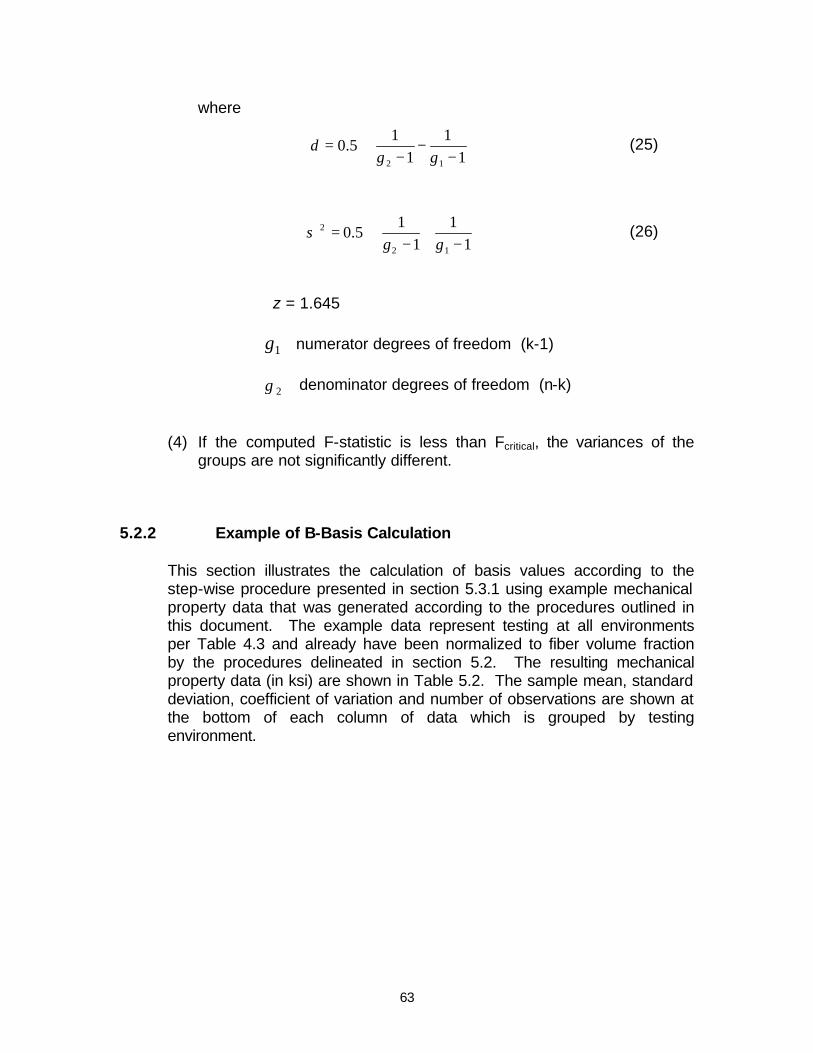
63
where
−−
−=
11
11
5.012 γγ
δ (25)
−+
−=
11
11
5.012
2
γγσ (26)
z = 1.645 1γ numerator degrees of freedom (k-1) 2γ denominator degrees of freedom (n-k)
(4) If the computed F-statistic is less than Fcritical, the variances of the groups are not significantly different.
5.2.2 Example of B-Basis Calculation
This section illustrates the calculation of basis values according to the step-wise procedure presented in section 5.3.1 using example mechanical property data that was generated according to the procedures outlined in this document. The example data represent testing at all environments per Table 4.3 and already have been normalized to fiber volume fraction by the procedures delineated in section 5.2. The resulting mechanical property data (in ksi) are shown in Table 5.2. The sample mean, standard deviation, coefficient of variation and number of observations are shown at the bottom of each column of data which is grouped by testing environment.
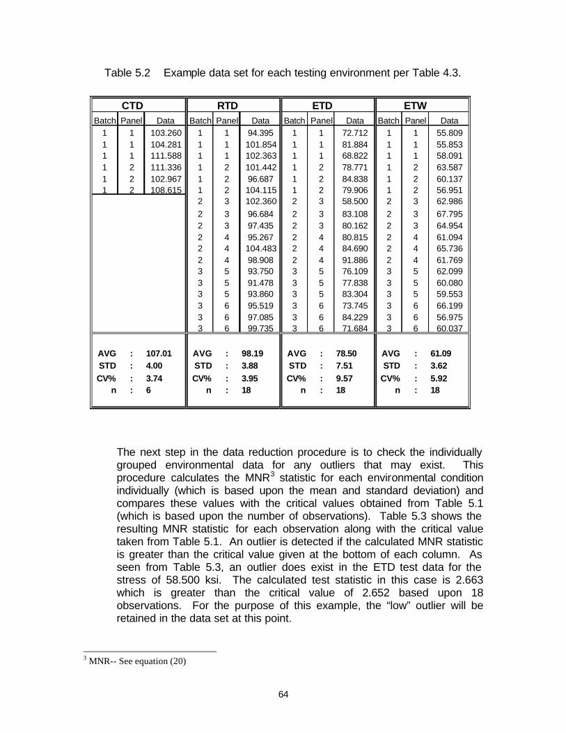
64
Table 5.2 Example data set for each testing environment per Table 4.3.
CTD RTD ETD ETWBatch Panel Data Batch Panel Data Batch Panel Data Batch Panel Data
1 1 103.260 1 1 94.395 1 1 72.712 1 1 55.8091 1 104.281 1 1 101.854 1 1 81.884 1 1 55.8531 1 111.588 1 1 102.363 1 1 68.822 1 1 58.0911 2 111.336 1 2 101.442 1 2 78.771 1 2 63.5871 2 102.967 1 2 96.687 1 2 84.838 1 2 60.1371 2 108.615 1 2 104.115 1 2 79.906 1 2 56.951
2 3 102.360 2 3 58.500 2 3 62.9862 3 96.684 2 3 83.108 2 3 67.7952 3 97.435 2 3 80.162 2 3 64.9542 4 95.267 2 4 80.815 2 4 61.0942 4 104.483 2 4 84.690 2 4 65.7362 4 98.908 2 4 91.886 2 4 61.7693 5 93.750 3 5 76.109 3 5 62.0993 5 91.478 3 5 77.838 3 5 60.0803 5 93.860 3 5 83.304 3 5 59.5533 6 95.519 3 6 73.745 3 6 66.1993 6 97.085 3 6 84.229 3 6 56.9753 6 99.735 3 6 71.684 3 6 60.037
AVG : 107.01 AVG : 98.19 AVG : 78.50 AVG : 61.09STD : 4.00 STD : 3.88 STD : 7.51 STD : 3.62CV% : 3.74 CV% : 3.95 CV% : 9.57 CV% : 5.92
n : 6 n : 18 n : 18 n : 18
The next step in the data reduction procedure is to check the individually grouped environmental data for any outliers that may exist. This procedure calculates the MNR3 statistic for each environmental condition individually (which is based upon the mean and standard deviation) and compares these values with the critical values obtained from Table 5.1 (which is based upon the number of observations). Table 5.3 shows the resulting MNR statistic for each observation along with the critical value taken from Table 5.1. An outlier is detected if the calculated MNR statistic is greater than the critical value given at the bottom of each column. As seen from Table 5.3, an outlier does exist in the ETD test data for the stress of 58.500 ksi. The calculated test statistic in this case is 2.663 which is greater than the critical value of 2.652 based upon 18 observations. For the purpose of this example, the “low” outlier will be retained in the data set at this point.
3 MNR-- See equation (20)

65
Table 5.3 Calculated MNR statistic for the environmentally grouped data.
Raw Data MNR Raw Data MNR Raw Data MNR Raw Data MNR103.260 0.936 94.395 0.977 72.712 0.771 55.809 1.460104.281 0.681 101.854 0.944 81.884 0.451 55.853 1.448111.588 1.144 102.363 1.075 68.822 1.289 58.091 0.830111.336 1.081 101.442 0.838 78.771 0.036 63.587 0.689102.967 1.010 96.687 0.387 84.838 0.844 60.137 0.265108.615 0.402 104.115 1.526 79.906 0.187 56.951 1.145
102.360 1.074 58.500 2.663 62.986 0.52396.684 0.388 83.108 0.614 67.795 1.85197.435 0.194 80.162 0.221 64.954 1.06695.267 0.753 80.815 0.308 61.094 0.000
104.483 1.621 84.690 0.824 65.736 1.28298.908 0.185 91.886 1.782 61.769 0.18693.750 1.143 76.109 0.318 62.099 0.27791.478 1.729 77.838 0.088 60.080 0.28093.860 1.115 83.304 0.640 59.553 0.42695.519 0.688 73.745 0.633 66.199 1.41197.085 0.285 84.229 0.763 56.975 1.13899.735 0.398 71.684 0.908 60.037 0.292
CTD
Critical Value Critical Value Critical Value Critical Value1.887 2.652 2.652 2.652
RTD ETD ETW
After the data is checked for outliers, a visual check should be performed on the environmentally grouped data to validate the assumption of normality following the procedures outlined in section 5.3.2. Figure 5.2 shows the data from Table 5.2 plotted against the standard normal curves for each environment tested. As seen in the figure, the normal model appears to closely represent the data across all represented environments and does not appear to cause any significant “engineering concerns”.

66
0 40 80 120 160Failure Stress (ksi)
0
0.2
0.4
0.6
0.8
1
Pro
bab
ility
of
Sur
viva
l
CTDRTDETDETWNormal Fit
Figure 5.2 Normalized fit of experimental data for each environment.
The next step in the data reduction process is the pooling of data across environments. The data from each environment is normalized using the sample mean from each environmental condition. Table 5.4 shows the resulting normalized data pooling all environments together. As seen from this method, all strength values then take-on a normalized value in the neighborhood of one. Also shown in Table 5.4 are the resulting mean, standard deviation, coefficient of variation and number of observations.

67
Table 5.4 Resulting pooled data after normalization procedure.
CTD RTD ETD ETWBatch Panel Data Batch Panel Data Batch Panel Data Batch Panel Data
1 1 0.965 1 1 0.961 1 1 0.926 1 1 0.9131 1 0.975 1 1 1.037 1 1 1.043 1 1 0.9141 1 1.043 1 1 1.042 1 1 0.877 1 1 0.9511 2 1.040 1 2 1.033 1 2 1.003 1 2 1.0411 2 0.962 1 2 0.985 1 2 1.081 1 2 0.9841 2 1.015 1 2 1.060 1 2 1.018 1 2 0.932
2 3 1.042 2 3 0.745 2 3 1.031
2 3 0.985 2 3 1.059 2 3 1.1102 3 0.992 2 3 1.021 2 3 1.0632 4 0.970 2 4 1.029 2 4 1.0002 4 1.064 2 4 1.079 2 4 1.0762 4 1.007 2 4 1.171 2 4 1.0113 5 0.955 3 5 0.970 3 5 1.0163 5 0.932 3 5 0.992 3 5 0.9833 5 0.956 3 5 1.061 3 5 0.9753 6 0.973 3 6 0.939 3 6 1.0843 6 0.989 3 6 1.073 3 6 0.9333 6 1.016 3 6 0.913 3 6 0.983
Pooled Average : 1.000Pooled Standard Dev. : 0.0649
Coeff. of Variation : 6.494Number of Observations : 60
Using the pooled data, the outlier and normality check is also conducted on the pooled data set. Table 5.5 shows the resulting MNR values for the pooled data set along with the critical value obtained from Table 5.1 (based upon 60 observations). As seen from table 5.5, the one outlier is still present in the data and will be retained for the purpose of this example. Figure 5.3 shows the visual check of the normal distribution with respect to the pooled data. As seen from Fig. 5.3, the normal model appears to closely represent the data across all pooled data and does not appear to cause any significant “engineering concerns”.
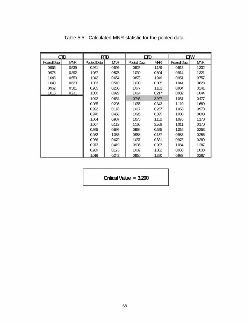
68
Table 5.5 Calculated MNR statistic for the pooled data.
Pooled Data MNR Pooled Data MNR Pooled Data MNR Pooled Data MNR0.965 0.539 0.961 0.595 0.923 1.189 0.913 1.3320.975 0.392 1.037 0.575 1.039 0.604 0.914 1.3211.043 0.659 1.042 0.654 0.873 1.949 0.951 0.7571.040 0.623 1.033 0.510 1.000 0.005 1.041 0.6280.962 0.581 0.985 0.236 1.077 1.181 0.984 0.2411.015 0.231 1.060 0.929 1.014 0.217 0.932 1.044
1.042 0.654 0.745 3.927 1.031 0.4770.985 0.236 1.055 0.843 1.110 1.6890.992 0.118 1.017 0.267 1.063 0.9730.970 0.458 1.026 0.395 1.000 0.0001.064 0.987 1.075 1.152 1.076 1.1701.007 0.113 1.166 2.558 1.011 0.1700.955 0.696 0.966 0.525 1.016 0.2530.932 1.053 0.988 0.187 0.983 0.2560.956 0.679 1.057 0.881 0.975 0.3890.973 0.419 0.936 0.987 1.084 1.2870.989 0.173 1.069 1.062 0.933 1.0381.016 0.242 0.910 1.390 0.983 0.267
Critical Value = 3.200
CTD RTD ETD ETW

69
0.6 0.8 1 1.2 1.4
Normalized Pooled Data
0
0.2
0.4
0.6
0.8
1
Pro
bab
ility
of
Sur
viva
lNormal FitPooled Data
Figure 5.3 Normalized fit of pooled data.
After the pooled data has been collected, the pooled sample mean and standard deviation may be computed (see Fig. 5.4). Using these values, the B and A basis values may be calculated for the pooled data. Using eqn. (17) - (18), the one sided tolerance limits may be calculated for a pooled sample size of 60. The values of these tolerance limits are
8066.26090.1
==
A
B
kk
which, combined with the sample mean and standard deviation, yield B and A basis values of [via eqn. (19)]
8177.08955.0
==
normal
normal
AB
Once these values are obtained, the B and A basis for each environmental condition may be obtained using the mean of each environment and the

70
pooled B and A basis values. Simple multiplication yields the B and A basis values for each environment as
Statistic
CTD RTD ETD ETW
B-Basis Value 95.827 87.930 70.298 54.711
A-Basis Value 87.504 80.293 64.192 49.959
It should be noted that even though A-basis numbers were calculated for this example, the number of specimens was more in accordance with the number recommended for B-basis calculations. For a less conservative A-basis allowable, the number of specimens can be increased to those given in Table 4.4.
5.3 Material Performance Envelope and Interpolation
Using the B-basis numbers generated in the previous example, a material performance envelope may be generated for the example material system by plotting these values as a function of temperature. Figure 5.5 shows the material performance envelope using the B-basis values generated in the previous example. As seen from Fig. 5.5, an envelope of material performance may be generated.
Since each specific aircraft application of the qualified material may have different Maximum Operational Limits (MOL) than those tested in the material qualification (which is usually the upper limit), some applications may require a reduced MOL. In this case, simple linear interpolation may be used to obtain the corresponding basis values at the new application MOL.

71
-100 -50 0 50 100 150 200
Temperature (o F)
20
40
60
80
100
120
B-B
asis
Str
eng
th V
alu
es (
ksi)
CTD
RTD
ETD
ETW
Material Performance Envelope
Figure 5.5 Material performance envelope.
This interpolation may be accomplished using the following simple relationships assuming TRTD < TMOL < TETD :
For the corresponding MOL “dry” basis value, the “interpolated” basis value using the qualification data is
( ) ( )
( )ETDRTD
MOLRTDETDRTDRTDMOL TT
TTBBBB
−−−
−=
(27)
where: BMOL = new application basis value interpolated to TMOL
BRTD = basis RTD strength value BETD = basis ETD strength value TRTD = RTD test temperature

72
TETD = ETD test temperature TMOL = new application MOL temperature
For the corresponding MOL “wet” basis value, the “interpolated” basis value using the qualification data is
( ) ( )
( )ETWCTD
MOLCTDETWCTDCTDMOL TT
TTBBBB
−−−
−=
(28)
where: BMOL = new application basis value interpolated to TMOL
BCTD = basis CTD strength value BETW = basis ETW strength value TCTD = CTD test temperature
TETW = ETW test temperature TMOL = new application MOL temperature
These equations may also be used for interpolated mean strengths as well as A-basis values with the appropriate substitutions. It should be noted that because unforeseen material property drop-offs with respect to temperature and environment can occur, extrapolation to a higher MOL should not be attempted without additional testing and verification. In addition, the interpolation equations shown above are practical for materials obeying typical mechanical behavior. In most cases, some minimal amount of testing may also be required to verify the interpolated values.
5.3.1 Interpolation Example
Using the basis values obtained in the previous example presented in section 5.3.2, this section provides an example of linear interpolations to a specific application environment less than the tested upper material limit used in qualification. Assuming a specific application environment of 150o F, Figure 5.6 depicts the linear interpolation of the B-basis design allowable to this environment. Using eqn. (27) and (28) along with the nominal testing temperatures (see Table 4.3), the interpolated basis values at 150o F become
ETD : BMOL = 75.106 ksi ETW : BMOL = 59.746 ksi

73
-100 -50 0 50 100 150 200
Temperature (o F)
20
40
60
80
100
120
B-B
asis
Str
en
gth
Val
ues
(ks
i)
CTD
RTD
ETD
ETW
Figure 5.6 Example of 150o F interpolation for B-basis values.
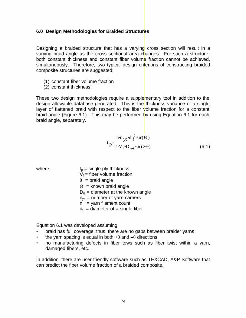
74
6.0 Design Methodologies for Braided Structures Designing a braided structure that has a varying cross section will result in a varying braid angle as the cross sectional area changes. For such a structure, both constant thickness and constant fiber volume fraction cannot be achieved, simultaneously. Therefore, two typical design criterions of constructing braided composite structures are suggested;
(1) constant fiber volume fraction (2) constant thickness
These two design methodologies require a supplementary tool in addition to the design allowable database generated. This is the thickness variance of a single layer of flattened braid with respect to the fiber volume fraction for a constant braid angle (Figure 6.1). This may be performed by using Equation 6.1 for each braid angle, separately.
(6.1)
where, tp = single ply thickness Vf = fiber volume fraction
θ = braid angle Θ = known braid angle DΘ = diameter at the known angle nyc = number of yarn carriers n = yarn filament count df = diameter of a single fiber
Equation 6.1 was developed assuming; • braid has full coverage, thus, there are no gaps between braider yarns • the yarn spacing is equal in both +θ and –θ directions • no manufacturing defects in fiber tows such as fiber twist within a yarn,
damaged fibers, etc. In addition, there are user friendly software such as TEXCAD, A&P Software that can predict the fiber volume fraction of a braided composite.
t pn n yc. d f
2. sin Θ( ).
2 V f. D Θ
. sin 2 θ.( ).

75
6.1 Thickness vs. Fiber Volume Fraction
Figure 6.1 Thickness vs. fiber volume fraction for a constant braid angle.
The thickness variances at ±30°, ±45° and ±60° braid angles are illustrated in Figure 6.2 for fiber volume fractions ranging from 30% to 70%. This illustration is for the 3.5” 6K 2-D 2X2 biaxial braided sleeve (208 yarn carriers). If the constant fiber volume fraction methodology is selected, in Figure 6.2, the vertical line passing through the selected fiber volume fraction will intersects the ±30°, ±45° and ±60° curves at the thickness of single layer corresponding to each braid angle. Similarly, if the constant thickness methodology is selected, the horizontal line passing through the selected thickness will intersects the ±30°, ±45° and ±60° curves at the fiber volume fraction of single layer corresponding to each braid angle.
6.2 Mechanical Property Distribution
Mechanical properties of a braid directly depend on the braid angle and the fiber volume fraction. In order to create a mechanical property database of braided composites, testing need to be conducted for different braid angles (i.e. ±30°, ±45° and ±60°) and fiber volume fractions (i.e. 49%, 57% and 65%). Therefore, two additional sub-matrices must be added to the test matrices shown in Table 4.3 through 4.5. One test batch of each low and high fiber volume fraction for the room temperature dry (RTD) testing must be conducted (Table 6.1). Instead of a single value at a particular fiber volume fraction, these two additional sub-matrices provide a distribution of the properties with respect to the selected fiber volume fraction range.
w x z
t P2
Vf (tp1)
w x z
t p1
Vf (tp2)

76
Figure 6.2 Single layer thickness variance of a 3.5” braid against the fiber volume fraction at ±30°, ±45° and ±60° braid angles.
0.00
0.01
0.02
0.03
0.04
0.05
0.06
0.20 0.30 0.40 0.50 0.60 0.70 0.80
Fiber Volume Fraction (%)
Sin
gle
Laye
r Thi
ckne
ss (i
n)
±30° & ±60°Braid±45° Braid
cons
tant
fibe
r vol
ume
fract
ion
constant thickness
3.5" Braid

77
Figure 6.3 Illustration of the material property extraction from the database for constant thickness methodology to obtain 0° tensile strength.
±30° Braid ±45° Braid ±60° Braid
σ30 (Vf1) σ45 (Vf2) σ60 (Vf3)
0
100
200
300
400
500
600
700
25 30 35 40 45 50 55 60 65
Braid Angle (deg)
Ten
sile
Str
engt
h (M
Pa)
σ30 (Vf1)
σ45 (Vf2)
σ60 (Vf3)
Mechanical Properties of Braid
Mechanical Properties of Structure
0
100
200
300
400
500
600
700
45 55 65 75
Fiber Volume Fraction (%)
Stre
ngth
(MPa
)
0
20
40
60
80
100
120
45 55 65 75Fiber Volume Fraction (%)
Stre
ngth
(MPa
)
0
50
100
150
200
250
300
45 55 65 75
Fiber Volume Fraction (%)St
reng
th (M
Pa)

78
Low fiber volume fraction can be obtained by removing a ply from the regular layup schedule and the high fiber volume fraction can be achieved by adding a ply to the regular layup schedule. Hence, the same mold can be used for panels with low, mid and high fiber volume fractions. Once the testing for the complete matrices are done for each braid angle, a distribution of each property with respect to the fiber volume fraction can be plotted as in Figure 6.4. The B-basis basis tolerance factor, kB, for the main test matrix with mid fiber volume fraction must be calculated as described in section 5.2.1. Then, the same tolerance factor must be used for both high and low fiber volume fraction test matrices (Figure 6.4).
Table 6.1 Complete test matrices development for a braided composite database.
Figure 6.4 B-basis design allowable calculation based on the statistical analysis.
TENSILE STRENGTH OF ±45° BRAID
25
27
29
31
33
35
37
45 50 55 60 65 70
Fiber Volume Fraction (%)
Stre
ngth
(ks
i)
Experimental
B-Basis
3 BatchesETW
1 BatchETD
1 Batch3 Batches1 BatchRTD
1 BatchCTD
High VfMid VfLow Vf
3 BatchesETW
1 BatchETD
1 Batch3 Batches1 BatchRTD
1 BatchCTD
High VfMid VfLow Vf
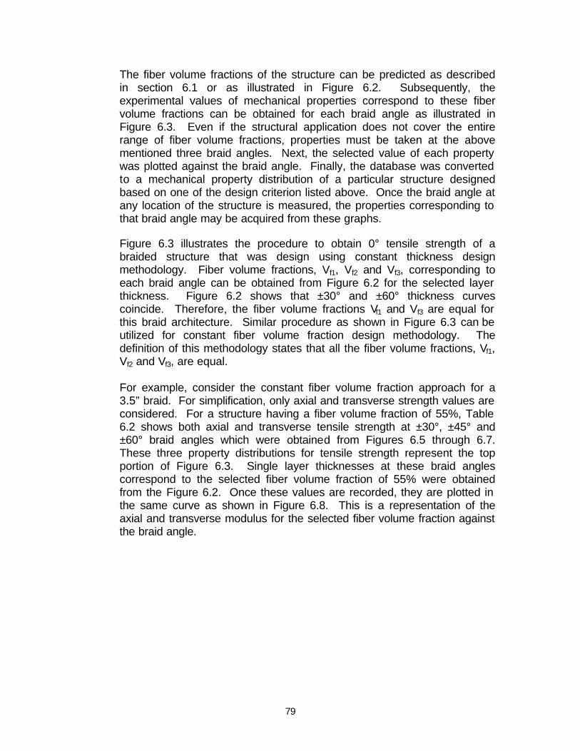
79
The fiber volume fractions of the structure can be predicted as described in section 6.1 or as illustrated in Figure 6.2. Subsequently, the experimental values of mechanical properties correspond to these fiber volume fractions can be obtained for each braid angle as illustrated in Figure 6.3. Even if the structural application does not cover the entire range of fiber volume fractions, properties must be taken at the above mentioned three braid angles. Next, the selected value of each property was plotted against the braid angle. Finally, the database was converted to a mechanical property distribution of a particular structure designed based on one of the design criterion listed above. Once the braid angle at any location of the structure is measured, the properties corresponding to that braid angle may be acquired from these graphs.
Figure 6.3 illustrates the procedure to obtain 0° tensile strength of a braided structure that was design using constant thickness design methodology. Fiber volume fractions, Vf1, Vf2 and Vf3, corresponding to each braid angle can be obtained from Figure 6.2 for the selected layer thickness. Figure 6.2 shows that ±30° and ±60° thickness curves coincide. Therefore, the fiber volume fractions Vf1 and Vf3 are equal for this braid architecture. Similar procedure as shown in Figure 6.3 can be utilized for constant fiber volume fraction design methodology. The definition of this methodology states that all the fiber volume fractions, Vf1, Vf2 and Vf3, are equal.
For example, consider the constant fiber volume fraction approach for a 3.5” braid. For simplification, only axial and transverse strength values are considered. For a structure having a fiber volume fraction of 55%, Table 6.2 shows both axial and transverse tensile strength at ±30°, ±45° and ±60° braid angles which were obtained from Figures 6.5 through 6.7. These three property distributions for tensile strength represent the top portion of Figure 6.3. Single layer thicknesses at these braid angles correspond to the selected fiber volume fraction of 55% were obtained from the Figure 6.2. Once these values are recorded, they are plotted in the same curve as shown in Figure 6.8. This is a representation of the axial and transverse modulus for the selected fiber volume fraction against the braid angle.

80
Figure 6.5 Axial and transverse tensile strength of ±30° braid.
Figure 6.6 Axial and transverse tensile strength of ±45° braid.
Figure 6.7 Axial and transverse tensile strength of ±60° braid.
0
5
10
15
20
25
30
35
40
45 55 65 75
Fiber Volume Fraction (%)
Str
en
gth
(ks
i)
Axial
Transverse
010
20304050
607080
90100
45 55 65 75
Fiber Volume Fraction (%)
Str
engt
h (k
si)
Axial
Transverse
0
20
40
60
80
100
45 55 65 75
Fiber Volume Fraction (%)
Stre
ngth
(ks
i)
Axial
Transverse

81
Table 6.2 Tensile strength properties for 3.5” braid at a fiber volume
fraction of 55%.
Braid Angle Single Layer Thickness (in)
Axial Tensile Strength (Msi)
Transverse Tensile Strength (Msi)
±30° 0.0205 78.6 14.0
±45° 0.0179 28.7 28.7
±60° 0.0205 14.0 78.6
Figure 6.8 Tensile strength vs. braid angle at the fiber volume fraction of 55%.
Once the braid angle at any location of the structure is measured, corresponding axial and transverse tensile strengths at that location are directly obtained from Figure 6.8. It is important to notice the thickness variance, when the constant fiber volume fraction methodology is followed (see Table 6.2). This procedure can be repeated for the rest of the properties.
0
15
30
45
60
75
90
25 35 45 55 65
Braid Angle (deg.)
Tens
ile S
treng
th (k
si.) Axial
Transverse

82
Appendix A
Example Panel Size Requirements

83
ASTM D3039 - Tensile Strength, Modulus, and Poisson’s Ratio
B-Basis Design Allowables for ±45° Braid in the 0° (warp) Direction
Required specimens are:
CD RTD HW HD
Strength 1x4 3x4 3x4 1x4
Strength, Modulus,
& Poisson’s Ratio
1x2 3x2 3x2 1x2
Recommended panel size:
Physical Test Strip
90°
0°
Subpanels 18.5”
10”
Preferred Reference Edge
Panel Dimensions
Layup Configuration: [0]n with a minimum thickness of 0.104”
Minimum Number of Panels:
Batch 1 2 3
Panels 3 2 2
Specimens 32 16 16
Number of Subpanels per Panel: 2

84
Combined Loading Compression – Compressive Strength and Modulus
B-Basis Design Allowables for ±45° Braid in the 0° (warp) Direction
Required specimens are:
CD RTD HW HD
Strength 1x4 3x4 3x4 1x4
Strength &
Modulus
1x2 3x2 3x2 1x2
Recommended Panel Size:
Physical Test Strip
90°
0°
Subpanels 18.5”
10”
Preferred Reference Edge
Panel Dimensions
Layup Configuration: [0]n with a minimum thickness of 0.104”
Minimum Number of Panels:
Batch 1 2 3
Panels 1 1 1
Specimens 32 16 16
Number of Subpanels per Panel: 3

85
ASTM D5379 – In-Plane Shear Strength and Modulus (Modified)
B-Basis Design Allowables for ±45° Braid
Required specimens are:
CD RTD HW HD
Strength 1x6 3x6 3x6 1x6
Modulus 1x2 3x2 3x2 1x2
Recommended Panel Size:
Physical Test Strip
90°
0°
Subpanels 18.5”
10”
Preferred Reference Edge
Panel Dimensions
Layup Configuration: [0]n with a minimum thickness of 0.104”
Minimum Number of Panels:
Batch 1 2 3
Panels 2 1 1
Specimens 44 22 22
Number of Subpanels per Panel: 4

86
ASTM D2344 - Short Beam Shear
B-Basis Design Allowables for ±45° Braid
Required specimens are:
CD RTD HW HD
Strength 3x6
Strength &
Modulus
Recommended Panel Size:
18.5”
10”
0°
90°
Preferred Reference Edge
Physical Test Strip
Subpanel
Panel Dimensions
Layup Configuration: [0]n with a minimum thickness of 0.104”
Minimum Number of Panels per batch: 1
Number of Subpanels per Panel: 1

87
ASTM D3039 - Tensile Strength, Modulus, and Poisson’s Ratio
B-Basis Design Allowables for ±60° Braid in the 0° (warp) Direction
Required specimens are:
CD RTD HW HD
Strength 1x4 3x4 3x4 1x4
Strength, Modulus,
& Poisson’s Ratio
1x2 3x2 3x2 1x2
Recommended panel size:
18.5”
12.5”
0°
90°
Preferred Reference Edge
Physical Test Strip
Subpanels
Panel Dimensions
Layup Configuration: [0]n with a minimum thickness of 0.104”
Minimum Number of Panels:
Batch 1 2 3
Panels 2 1 1
Specimens 32 16 16
Number of Subpanels per Panel: 2

88
ASTM D3039 - Tensile Strength, Modulus, and Poisson’s Ratio
B-Basis Design Allowables for ±60° Braid in the 90° (fill) Direction
Required specimens are:
CD RTD HW HD
Strength 1x4 3x4 3x4 1x4
Strength, Modulus,
& Poisson’s Ratio
1x2 3x2 3x2 1x2
Recommended panel size:
18.5”
12.5”
0°
90°
Preferred Reference Edge
Physical Test Strip
Subpanel
Panel Dimensions
Layup Configuration: [0]n with a minimum thickness of 0.104”
Minimum Number of Panels:
Batch 1 2 3
Panels 3 2 2
Specimens 32 16 16
Number of Subpanels per Panel: 1

89
Combined Loading Compression – Compressive Strength and Modulus
B-Basis Design Allowables for ±60° Braid in the 0° (warp) Direction
Required specimens are:
CD RTD HW HD
Strength 1x4 3x4 3x4 1x4
Strength &
Modulus
1x2 3x2 3x2 1x2
Recommended Panel Size:
Physical Test Strip
90°
0°
Subpanels 18.5”
12.5”
Preferred Reference Edge
Panel Dimensions
Layup Configuration: [0]n with a minimum thickness of 0.104”
Minimum Number of Panels:
Batch 1 2 3
Panels 1 1 1
Specimens 32 16 16
Number of Subpanels per Panel: 3
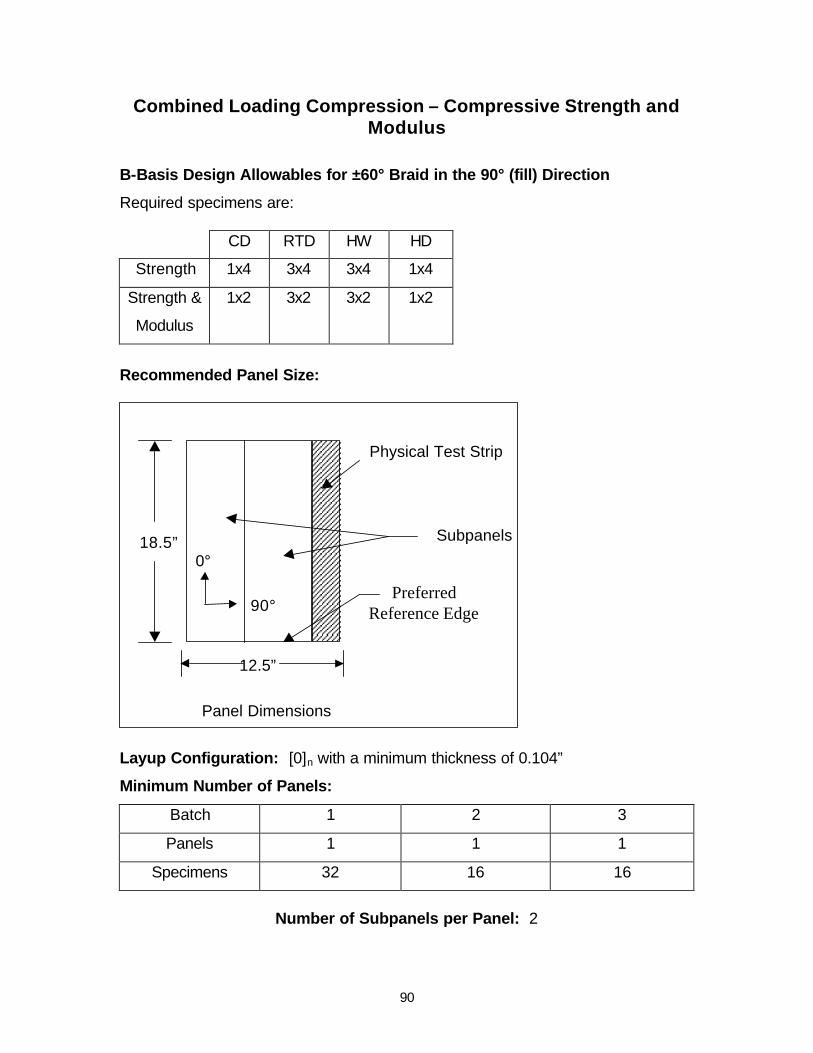
90
Combined Loading Compression – Compressive Strength and Modulus
B-Basis Design Allowables for ±60° Braid in the 90° (fill) Direction
Required specimens are:
CD RTD HW HD
Strength 1x4 3x4 3x4 1x4
Strength &
Modulus
1x2 3x2 3x2 1x2
Recommended Panel Size:
Physical Test Strip
90°
0°
Subpanels 18.5”
12.5”
Preferred
Reference Edge
Panel Dimensions
Layup Configuration: [0]n with a minimum thickness of 0.104”
Minimum Number of Panels:
Batch 1 2 3
Panels 1 1 1
Specimens 32 16 16
Number of Subpanels per Panel: 2

91
ASTM D5379 – In-Plane Shear Strength and Modulus
B-Basis Design Allowables for ±60° Braid
Required specimens are:
CD RTD HW HD
Strength 1x6 3x6 3x6 1x6
Modulus 1x2 3x2 3x2 1x2
Recommended Panel Size:
Physical Test Strip
90°
0°
Subpanels 18.5”
10”
Preferred Reference Edge
Panel Dimensions
Layup Configuration: [0]n with a minimum thickness of 0.104”
Minimum Number of Panels:
Batch 1 2 3
Panels 2 1 1
Specimens 44 22 22
Number of Subpanels per Panel: 4

92
ASTM D2344 - Short Beam Shear
B-Basis Design Allowables for ±60° Braid
Required specimens are:
CD RTD HW HD
Strength 3x6
Strength &
Modulus
Recommended Panel Size:
18.5”
12.5”
0°
90°
Preferred Reference Edge
Physical Test Strip
Subpanel
Panel Dimensions
Layup Configuration: [0]n with a minimum thickness of 0.104”
Minimum Number of Panels per batch: 1
Number of Subpanels per Panel: 1

93
Appendix B
Example Panel Manufacturing Procedure Using RTM

94
BRAIDED PANEL MANEUFACTURING IN RTM TOOL PREPERATION: B.1. The tool is cleaned with Acetone (CH3COCH3). B.2. Apply 4-5 coats of C mold sealer
• Soak a clean, lint free, 100% woven cloth with sealer (FREKOTE B-15) until it is wet, but not dripping.
• Starting at one end of the mold surface, wipe on a smooth, continues, wet film. (Only a thin wet film is required.) As the sealer dries rapidly, care should be taken not to wipe back over the area just coated once the solvents have flashed off.
• If coating a large area, the application cloth may require re-soaking several times to maintain the thin, wet film.
• Allow at least 20 to 30 minutes between each coat, at room temperature. • The final coating will cure within 24 hours at room temperature. The cure can be
accelerated by heating the mold at 200o F or above for 1 hour.
Figure B.1: Aluminum mold for the panel manufacturing.
B.3. Apply FREKOTE NC 44 ( or 770-NC) releasing agent
• Follow the same procedure as in step 2. • Apply 4 coats for the first time, and 2 coats per use of mold. • Wait 5 to 10 minutes between each coat.
B.4. The Silicon sealer (O-ring type) is placed inside the slot
• Apply a high temperature automotive Silicon sealer (VersaChem Mega Copper) on the surface of the slot (Figure B.1).
• Smear thin bead with scrap Silicon gasket. • Spray the sealer with water mist. • Wait for 10 minutes. • Insert the Silicon sealer into the slot. • Wait 2 to 3 hours for the silicon gasket to cure.
Female Mold Male Mold
Slot

95
LAYUP
Figure B.2: Cutting the preform to a given braid angle using an Aluminum cylinder.
B.5. Cut the braided Carbon layers (Must be performed in the Layup Room)
• Wear white cotton gloves. • Slide the braided sleeve through the appropriate aluminum cylinder. • Holding the end of the braid tight, pull the sleeve and lock the braid angle. • Using the green flashbreaker pressure sensitive tape, secure the braid angle as shown in
Figure B.2. • Cut the top tape along its centerline and separate the braided sleeve. • Slide the braided sock out of the aluminum cylinder.
(Make sure all the tapes are still attached to the sock.) • Cut the lengthwise tape in half and open the braid. • Repeat step 6 until the appropriate layers of braid are obtained.
Figure B.3: Cross-section of the mold
Aluminum Male Mold
Aluminum Female Mold
High Temperature Silicon Seal (O-Ring Type)
Braided Carbon Layers
Tape
Aluminum Cylinder
BraidedSleeve

96
B.6. Place the preform in the mold. • Trim the green tape if necessary. • Place each layer against the reference edge. • Make sure no ply wrinkling or foreign materials are present. • Make sure the fiber distortion is no more than ±5°. • Close the mold (Figure B.3).
RESIN INJECTION B.7.Place the Aluminum mold inside the 150 ton Twin Deck Pneumatic Press.
• Set the force to 200,000 lbs. and place the mold between the heated platens of the press (Figure B.4)
• Set the temperature to 340o F and insert the tool temperature thermocouple. • Wait until the tool temperature stabilizes at 340o F, before injecting the resin.
Figure B.4: Resin Transfer Molding Setup. B.8. Prepare the Heated RTM Pump for resin injection
• Connect the air pressure source to the RTM pump. • Remove PR 520 resin can from the refrigerated storage 24 hours before injecting it. • Make sure all air regulators and bleed-type valves are closed. • Open the air valve in main line. • Set Ram air regulator to 15-18 psi. (lower gage) • Set pump air regulator to 0 psi. (upper gage) • Set the Ram plate temperature and the Hose temperature to 200° F.
Regulated Air Pressure Source
Heated RTM Pump
Resin
150 TON TWIN DECK PNEUMATIC PRESS
Vacuum pump
Aluminum Mold
Top Platen
Bottom Platen
Needle Valve
Vent Valve
Clamp 1
Clamp 2
Heated Hose

97
B.9. Check the tool for vacuum integrity. • Connect one end of the high temperature tube (3 to 4 ft.) to the vacuum source and the
other end to the outlet of the mold. • Switch on the vacuum pump. • Insert the vacuum gage into the inlet of the mold. • Open the vacuum valve and hold it for 10 minutes. • Close the vacuum valve and wait for 5 minutes. • Decay rate must be less than 2 Hg/5 minutes. If the decay rate is higher than 2 Hg/5
minutes, check all the connections and/or repeat step 4 until the specified vacuum integrity is obtained.
• Remove the inlet vacuum gage and connect the heated hose to the inlet of the mold. • Turn the vacuum pump on.
B.10. Resin injection • Close the vent valve halfway. • Increase the initial injection pressure to 80 psi. • Open the ball valve and slowly open the needle valve. • Let the resin flow at the outlet until the bubbles are disappeared. • Clamp the outlet tube 6-inch. away from the mold, before the resin flow reaches the vent
valve. • Disconnect the tube from the vent valve. • Increase the injection pressure to 100 psi. • Decrease the Hose temperature to 160° F and turn off the Ram plate temperature. • Increase the press temperature to 370o F.
CURE PROFILE
B.11. Gel time
• Maintain the injection pressure between 75 and 125 psi. until 30 minutes after the tool temperature reaches 365° F.
• Clamp the injection line. • Turn off the Hose temperature. • Cut the injection tube between clamp 2 and the needle valve, and remove the heated
hose. • Mold must maintain the vacuum integrity throughout the procedure.
B.12. Cure the resin for 2 hours at 365°F.
• Tool must be at 365°F for 2 hours, after the gel time, for the complete cure. • After the cure cycle is complete, cool down the mold. (keep the press closed)
B.13. Remove the part.
• Open the press after the tool temperature is reached 200°F. • Remove the part, before it reaches the room temperature. • Write the panel ID, reference edge, and the 0° and 90° direction on the panel.
NOTE: The RTM setup card provided at the end of Appendix B is only an example for 2x2
biaxially braided carbon and PR520 one-part epoxy resin system. The cure profile and injection requirements may vary according to the resin system. The layup schedule may also be varied according to the panel thickness and the fiber volume fraction. The panel inspection sheet may also be altered based on the certification requirements. However, the same setup card format MUST be followed for all the panels manufactured.
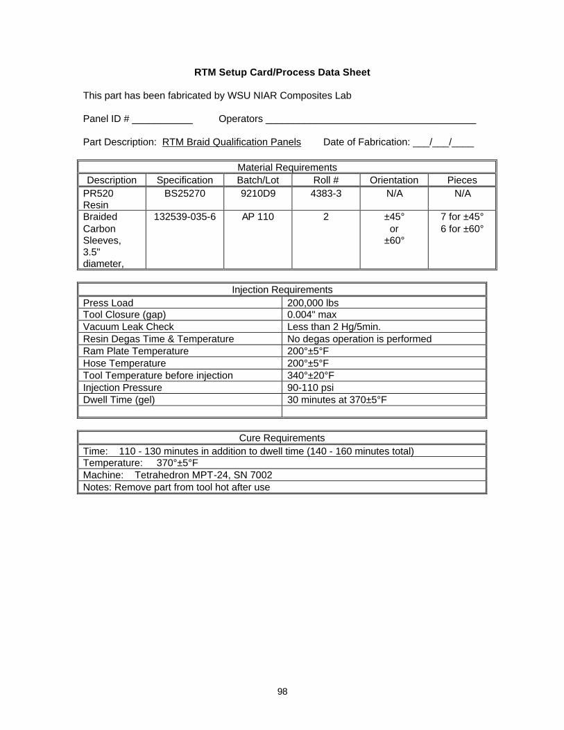
98
RTM Setup Card/Process Data Sheet This part has been fabricated by WSU NIAR Composites Lab Panel ID # ___________ Operators ______________________________________ Part Description: RTM Braid Qualification Panels Date of Fabrication: ___/___/____
Material Requirements Description Specification Batch/Lot Roll # Orientation Pieces
PR520 Resin
BS25270 9210D9 4383-3 N/A N/A
Braided Carbon Sleeves, 3.5" diameter,
132539-035-6 AP 110 2 ±45° or
±60°
7 for ±45° 6 for ±60°
Injection Requirements
Press Load 200,000 lbs Tool Closure (gap) 0.004" max Vacuum Leak Check Less than 2 Hg/5min. Resin Degas Time & Temperature No degas operation is performed Ram Plate Temperature 200°±5°F Hose Temperature 200°±5°F Tool Temperature before injection 340°±20°F Injection Pressure 90-110 psi Dwell Time (gel) 30 minutes at 370±5°F
Cure Requirements Time: 110 - 130 minutes in addition to dwell time (140 - 160 minutes total) Temperature: 370°±5°F Machine: Tetrahedron MPT-24, SN 7002 Notes: Remove part from tool hot after use

99
Manufacturing Procedure Initial
01) Remove PR520 resin from freezer 24 hours prior to use 02) Preheat the press to 340°F. Set the load at 200,000 lbs. 03) WASH YOUR HANDS. Clean the mold with nylon wedges and moistened cotton towels. Do not use acetone unless absolutely necessary because acetone will remove release agent from the mold. Apply a thin layer of MONO-COAT E300 release agent all surfaces of the mold. Allow at least 30 minutes for the release agent to cure at room temperature.
04) THIS STEP MUST BE PERFORMED IN THE LAYUP ROOM. WASH YOUR HANDS. Wear white cotton gloves. Using GREEN flashbreaker pressure sensitive tape to secure the braid angle in appropriate diameter aluminum mandrel; cut 6 layers using the 4.28 in diameter mandrel for the ±60° panels or 7 layers using the 3.5 in diameter mandrel for the ±45° panels. Check each appropriate box below when finished laying up each ply. Place the preform in the mold and close the mold.
±45° panel ±60° panel 1. 1. 2. 2. 3. 3. 4. 4. 5. 5. 6. 6. 7.
05) Attach the fittings to the mold. Place the mold in the press and check vacuum integrity. Decay rate must be less than 2 Hg/5minutes.
06) Make sure all air regulators and bleed-type air valves are closed 07) Set Ram air regulator to 15-18 psi (lower gauge) 08) Set Pump air regulator to 0 psi (upper gauge) 09) Set Ram plate temperature to 200°F 10) Set Hose temperature to 200°F 11) Connect heated hose to the tool Wait for the Hose to reach 200°F, Ram Plate to reach 200°F, and tool to reach 340°+20/-0°F
12) Increase the air pressure on upper gauge (pump) so that the digital output shows 75-125 psi (100 psi nominal).
13) Open ball valve (red lever) and slowly open the needle valve to adjust the desired flowrate.
14) Clamp the outlet when the resin appears in the outlet. Turn off vacuum pump and Ram Plate heater. Lower the Hose temperature to 160°F.
15) Increase press temperature to 375°F by advancing to segment 2 16) Wait for 30 minutes after the tool thermocouple reaches 365°F. The resin has reached gel point at this time. Record the endpoints below. During this time, the digital pressure reading must be at 75-125 psi.
Time Temperature (°F) Start Gel Gel Complete 17) Clamp injection line, turn off Hose heater, and disconnect Heated Hose from the tool.

100
18) Complete cure is attained 140-160 minutes after the tool thermocouple reaches 365°F (or 110-130 minutes after gel point). Record the endpoints below. Cool down press at 1°-8°F/minute after full cure.
Time Temperature (°F) Start Cure Cure Complete 19) Remove tool from the press after tool has cooled down to below 160°F 20) Using a silver color pen, write the Panel ID #, 0° and 90° directions on the panel.

101
Final Panel Inspection
Part Description: RTM Braid Qualification Panels Unit # __________________ Inspector: _______________________________ Date: __________________
Inspection Procedures and Requirements Initial
Verify that all the information in RTM Setup Card/Process Data Sheet has been filled out.
Verify that the cure profile (temperature) is according to RTM Setup Card/Process Data Sheet.
Verify that all temperature measuring devices have been calibrated and certified per BS23934
Verify that the part thickness is .120±.004 inches for ±45° panels or .119±.004 inches for ±60° panels. Measure the thickness using a ball-ball micrometers.
Verify that there is no resin starvation or dry area. Verify that there is no ply wrinkles. Verify that there is no abrasion, indentation, or scratches. Verify that there is no edge voids. Verify that there is no resin ridges higher than 0.003 inch Verify that there is no foreign material larger than 0.75 in2 Verify that there is no fiber distortion of more than ±5° Verify that there is no surface depression of more than 0.009 inch deep. Surface depression between 0.005 to 0.009 inch is acceptable up to 1.0 inch length. Surface depression of less than 0.005 inch is acceptable regardless of quantity and length.
Verify that the part warpage is less than 0.15 inch. Measurement is made at the highest point on the panel with the panel placed on a precision granite table.
Verify that panel (only the marked area) passes NDI requirements Any deviation from the above requirements must be recorded in the table below.
Deviations ________________________________________________________________________ ________________________________________________________________________ ________________________________________________________________________ ________________________________________________________________________ ________________________________________________________________________

102
Appendix C
Combined Loading Compression (CLC) Proposed Standard
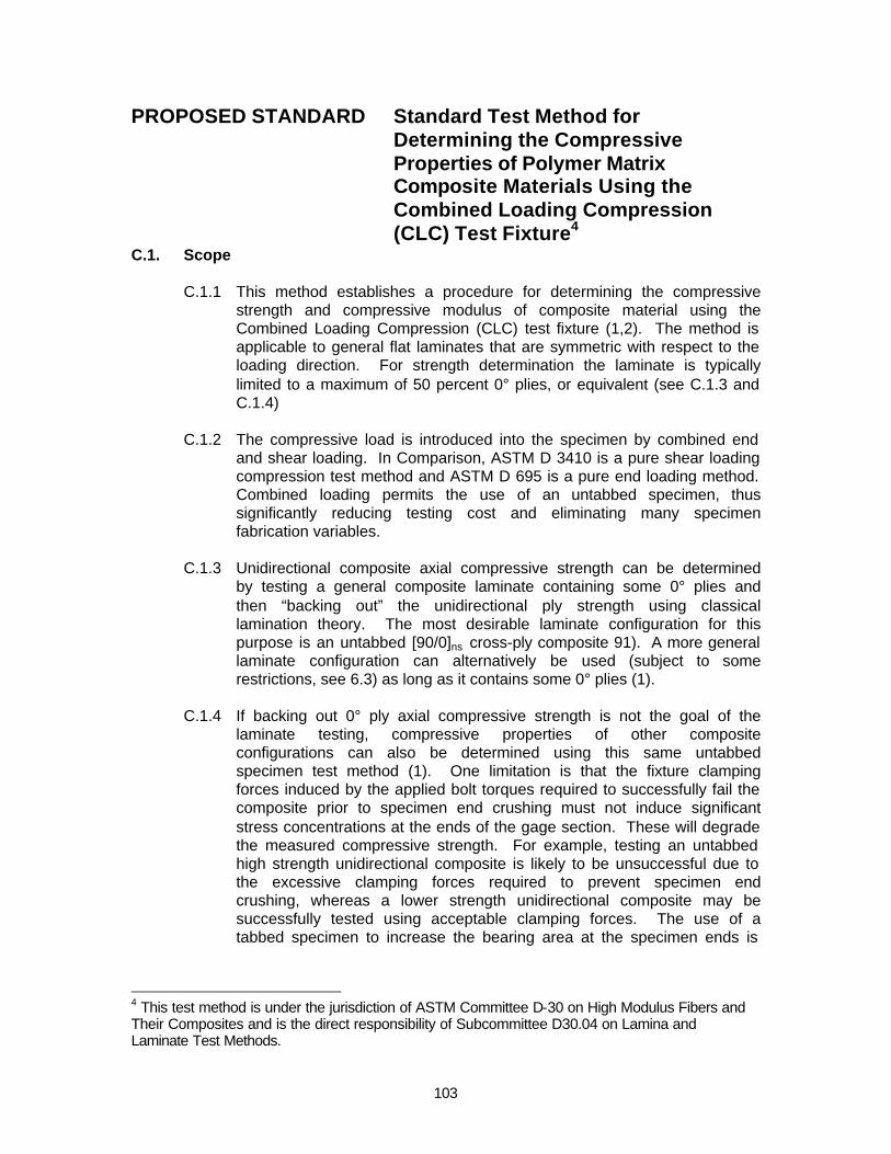
103
PROPOSED STANDARD Standard Test Method for Determining the Compressive Properties of Polymer Matrix Composite Materials Using the Combined Loading Compression (CLC) Test Fixture4
C.1. Scope
C.1.1 This method establishes a procedure for determining the compressive strength and compressive modulus of composite material using the Combined Loading Compression (CLC) test fixture (1,2). The method is applicable to general flat laminates that are symmetric with respect to the loading direction. For strength determination the laminate is typically limited to a maximum of 50 percent 0° plies, or equivalent (see C.1.3 and C.1.4)
C.1.2 The compressive load is introduced into the specimen by combined end
and shear loading. In Comparison, ASTM D 3410 is a pure shear loading compression test method and ASTM D 695 is a pure end loading method. Combined loading permits the use of an untabbed specimen, thus significantly reducing testing cost and eliminating many specimen fabrication variables.
C.1.3 Unidirectional composite axial compressive strength can be determined
by testing a general composite laminate containing some 0° plies and then “backing out” the unidirectional ply strength using classical lamination theory. The most desirable laminate configuration for this purpose is an untabbed [90/0]ns cross-ply composite 91). A more general laminate configuration can alternatively be used (subject to some restrictions, see 6.3) as long as it contains some 0° plies (1).
C.1.4 If backing out 0° ply axial compressive strength is not the goal of the
laminate testing, compressive properties of other composite configurations can also be determined using this same untabbed specimen test method (1). One limitation is that the fixture clamping forces induced by the applied bolt torques required to successfully fail the composite prior to specimen end crushing must not induce significant stress concentrations at the ends of the gage section. These will degrade the measured compressive strength. For example, testing an untabbed high strength unidirectional composite is likely to be unsuccessful due to the excessive clamping forces required to prevent specimen end crushing, whereas a lower strength unidirectional composite may be successfully tested using acceptable clamping forces. The use of a tabbed specimen to increase the bearing area at the specimen ends is
4 This test method is under the jurisdiction of ASTM Committee D-30 on High Modulus Fibers and Their Composites and is the direct responsibility of Subcommittee D30.04 on Lamina and Laminate Test Methods.
104
possible, but not desirable as tabs also induce unacceptable stress concentrations at the ends of the gage section.
C.1.5 This standard does not purport to address all of the safety problems, if
any, associated with its use. It is the responsibility of the user of the standard to establish appropriate safety and health practices and determine the applicability of regulatory limitations prior to use.
C.1.6 The values stated in either inch-pound units or SI units are to be regarded
separately as standard. Within the text the SI units are shown in brackets. The values stated in each system are not exact equivalents; therefore, each system must be used independently of the other. Combining values from the two systems may result in nonconformance with the standard.
Note 1 – Additional procedures for determining compressive properties of polymer matrix composites may be found in ASTM Test Methods D3410, D5467, and D695.
C.2. Reference Documents
C.2.1 ASTM Standards
D695 Test method for Compressive Properties of Rigid Plastics D888 Definitions of Terms Relating to Plastics D2734 Test Methods for Void Content of Reinforced Plastics D3171 Test methods for Fiber Content of Resin-Matrix Composites by
Matrix Design D3410 Test Methods for Compressive Properties of Polymer Matrix
Composite Materials with Unsupported Gage Section by Shear Loading
D3878 Terminology of High-Modulus Reinforced Fibers and their Composites
D5229 Test Method for Moisture Absorption Properties and Equilibrium Conditioning of Polymer Matrix Composite Materials
D5467 Test Method for Compressive Properties of Unidirectional-Polymer Matrix Composites Using a Sandwich Beam
E4 Practices for Load Verification of Testing Machines E6 Terminology Relating to Methods of Mechanical Testing E83 Practice for Verification and Classification of Extensometers E111 Test Method for Young’s Modulus, Tangent Modulus, and
Chord Modulus E122 Practice for Choice of Sample Size to Estimate a Measure of
Quality for a Lot or Process E132 Test Method for Poisson’s Ratio at Room Temperature E177 Practice for Use of the Terms Precision and Bias in ASTM
Test Methods E251 Test Methods for Performance Characteristics of Bonded
Resistance Strain Gages

105
E456 Terminology Relating to Quality and Statistics E1237 Practice for Installation of Bonded Resistance Strain Gages E1309 Guide for the Identification of Composite Materials in
Computerized Material Property Databases E1313 Guide for the Development of Standard Data Records for
Computerization of Material Property Databases E1434 Guide for the Development of Standard Data Records for
Computerization of Mechanical Test Data for High-Modulus Fiber-Reinforced Composite Materials
E1471 Guide for the Identification of Fibers, Fillers, and Core Materials in Computerized Material Property Databases
C.2.2 Other Documents:
ANSI Y14.5M-1982 ANSI/ASME B46.1-1985
C.3. Terminology
Terminology D3878 defines terms relating to high-modulus fibers and their composites. Terminology D883 defines terms relating to plastics. Terminology E6 defines terms relating to mechanical testing. Terminology E456 and Practice E177 define terms relating to statistics. In the event of a conflict between terms, Terminology D3878 Shall have precedence over the other terminology standards.
C.3.1 Descriptions of Terms Specific to the Standard:
C.3.1.1 nominal value, n-a value, existing in name only, assigned to a
measurable property for the purpose of convenient designation. Tolerances may be applied to a nominal value to define an acceptable range for the property.
C.3.1.2 orthotropic material, n-a material with a property of interest that,
at a given point, posses three mutually perpendicular planes of symmetry defining the principle material coordinate system for that property.
C.3.1.3 principal material coordinate system, n-a coordinate system with
axes that are normal to the planes of symmetry that exist within the material.
C.3.1.4 reference coordinate system, n-a coordinate system for
laminated composites used to define ply orientations. One of the reference coordinate system axes (normally the Cartesian x-axis) is designated the reference axis, assigned a position, and the ply principal axis of each ply in the laminate is referenced relative to the reference axis to define the ply orientation for that ply.

106
C.3.1.5 specially orthotropic, adj-a description of an orthotropic material as viewed in its principal material coordinate system. In laminated composites a specially orthotropic laminate is a balanced and symmetric laminate of the [0i/90j]ns family as viewed from the reference coordinate system, such that the membrane-bending coupling terms of the stress-strain relation are zero.
C.3.1.6 transition strain, etransition, n-the strain value at the mid-range of
the transition region between the two essentially linear portions for a bilinear stress-strain or strain-strain curve (a transverse strain-longitudinal strain curve as used for determining Poisson’s ratio).
C.3.2 Symbols:
3.2.1 A – cross-sectional area of specimen in gage section, 3.2.2 By – percent bending in specimen, 3.2.3 CV – sample of coefficient of variation, in percent, 3.2.4 Ex – modulus of elasticity in the test direction, 3.2.5 Fcu – ultimate compressive strength, 3.2.6 Gxz – through-thickness shear modulus of elasticity, 3.2.7 h – coupon thickness, 3.2.8 w – coupon width, 3.2.9 i, j, n – as used in a layup code, the number of repeats for a ply or
group of plies of material 3.2.10 l g – specimen gage length, 3.2.11 s – as used in a lay-up code, denotes that the preceding ply
description for the laminate is repeated symmetrically about its midplane,
3.2.12 n – number of specimens, 3.2.13 P – load carried by test specimen 3.2.14 Pf – load carried by test specimen at failure, 3.2.15 Pmax – maximum load to failure, 3.2.16 sn-1 – sample standard deviation, 3.2.17 w – coupon width, 3.2.18 xi – measured or derived property, 3.2.19 x – Sample mean (average), 3.2.20 ε – Indicated normal strain from strain transducer, 3.2.21 σc –Compressive normal stress, and 3.2.22 νc –Compressive Poisson’s ratio.
C.4. Summary of Test Method
The test fixture shown in Figure C.1 is used to test the untabbed, straight-sided composite specimen of rectangular cross section shown schematically in Figure C.2. The typical specimen is 5.5 in. (140 mm) long and 0.5 in. (12.7 mm) wide, having and unsupported (gage) length of 0.5 in. (12.7 mm) when installed in the fixture. This 0.5 in. (12.7 mm) gage length provides sufficient space to install bonded strain gages when they are required. The fixture, which subjects the

107
specimen to combined end- and shear-loading, is itself loaded in compression between flat platens in a universal testing machine. Load-strain data are collected until failure occurs (or until a specified strain level is achieved if only compressive modulus is being determined).
C.5. Significance and Use
This test method is designed to produce compressive property data for material specifications, research and development, quality assurance, and structural design and analysis. When specific laminates are tested (primarily of the [90/0]ns family, although other laminates containing a maximum of 50 percent 0° plies can be used), the data are frequently used to “back out” 0° ply strength, using lamination theory to calculate an 0° unidirectional lamina strength (1,2). Factors that influence the compressive response and should therefore be reported include the following: material, methods of material preparation and lay-up, specimen stacking sequence, specimen preparation, specimen conditioning, environment of testing, specimen alignment and gripping, speed of testing, time at temperature, void content, and volume percent reinforcement. Properties, in the test direction, that may be obtained from this test method include:
C.5.1 Ultimate compressive strength, C.5.2 Ultimate compressive strain, C.5.3 Compressive (linear or chord) modulus of elasticity, C.5.4 Poisson’s ratio in compression, and C.5.5 Transition strain
C.6. Interferences
C.6.1 Due to partial end loading of the specimen in this test method, it is important that the ends of the specimen be machined parallel to each other and perpendicular to the long axis of the coupon. Improper preparation may result in premature end crushing of the specimen during loading, potentially invalidating the test.
C.6.2 Erroneous compressive strengths will be produced due to Euler column
buckling if the specimen is too thin in relation to the gage length (see C.8.2). In such cases the specimen thickness must be increased or the gage length reduced. Buckling can usually only be detected by the use of back-to-back gages mounted on the faces of the specimen. It is not visually obvious, or by examining the specimen failure mode.
C.6.3 Continuous-fiber-reinforced laminates having more that 50% axially
oriented (0°) plies may require higher than acceptable fixture clamping forces to prevent end crushing. Excessive clamping forces induce local stress concentrations at the ends of the gage section that may produce erroneously low strength results (see C.9.2.11). Therefore, such specimens are considered nonstandard.
C.6.4 If the outermost plies of the laminate are oriented at 0°, the local stress
concentrations at the ends of the specimen gage section may lead to
108
premature failure of these primary load-bearing plies, producing erroneously low laminate strength results. This is particularly true for specimens with low numbers of plies, since then the outer plies represent a significant fraction of the total number of plies (1).
C.7. Apparatus and Supplies
C.7.1 Micrometers. 0.20 in. (5.1 mm) nominal diameter double ball for
measuring thickness and 0.25 in. (6.4 mm) diameter flat-flat for measuring width, suitable for reading to 0.0001 in. (0.0025 mm) accuracy.
C.7.2 Testing Machine. A calibrated testing machine shall be used which can
be operated at constant crosshead speed over the specified range. The test machine mechanism shall be essentially free from inertial lam at the crosshead speeds specified. The machine shall be equipped with an appropriate load-measuring device (e.g., a load cell). The accuracy of the test machine shall be in accordance with ASTM E 4.
C.7.3 Environmental Chamber. A chamber capable of enclosing the test fixture
and specimen while they are mounted in the testing machine, and capable of achieving the specified heating/coling rates, test temperatures and environments, shall be used when non-ambient conditions are required during testing.
C.7.4 Compression Fixture. The test fixture defined in Figre 1 shall be used.
Detailed drawings are available from ASTM. This fixture introduces a controllable ratio of end loading and shear loading into the specimen.
C.7.5 Data Acquisition Equipment. Equipment capable of recording load and
strain data is required. C.8. Test Specimen
The Combined Loading Compression (CLC) test specimen is a simple, untabbed, rectangular strip of the laminate to be tested, as shown in Figure C.2. Specimen dimensions and tolerances must be compliant with the requirements on Figure C.2. If the axial strain is to be measured (e.g., to monitor specimen bending, to determine the axial compressive modulus, or to obtain a stress-strain curve), two single-element axial strain gages or similar transducers are typically mounted back-to-back on the faces of the specimen, in the center of the gage section (see 10.2, 10.3). C.8.1 Specimen Width. The standard nominal width shall be 0.5 in. (12.7 mm).
However, other widths may be used, up to the maximum accommodated by the fixture (1.2 in., i.e., 30 mm), if required.
C.8.2 Specimen Thickness. The specimen thickness is arbitrary, but some
limitations must be imposed to preclude Euler column buckling of the specimen. Equation (C.1) may be used to estimate the minimum thickness to be used for the strength determinations, depending on a number of factors including gage length. The specimen can be thinner if
109
only modulus is being determined, as the required load range may then be significantly lower than the buckling load.
−
≥
cu
c
xz
cu
g
FE
GF
lh
2.119069.0
(C.1)
h = specimen thickness, in. (mm) l g = length of gage section, in. (mm) Fcu = expected ultimate compressive strength, psi (MPa) Ec = expected compressive modulus, psi (MPa) Gxz = through-the thickness (interlaminar) shear modulus,
psi (MPa)
Equation (C.1) may be rewritten as
xz
g
c
cr
GE
IA
EF2
22
2
2.1 π
π
+
=l
(C.2)
where:
Fcr = predicted Euler buckling stress, psi (MPa) A = specimen cross-sectional are, in.2 (mm2) I = minimum moment of inertia of specimen cross
section
Equation (C.2) can be used to estimate the applied stress Fcr on the test specimen at which Euler buckling is predicted to occur for the specific specimen configuration of interest. This value can then be compared to the expected compressive strength of the laminate.
A value of the laminate through-the thickness (interlaminar) shear modulus, Gxz, as required in Equations (C.1) and (C.2), may not be available in the form of experimental data. In this case, an estimate can be made using a simple rule-of-mixtures relation. For example, for a [90/0]ns laminate this value can be estimated as
9023012 VGVGGxz += (C.3)
where:
G12 = in-plane shear modulus of the 0° plies, psi (MPa) G23 = through-the-thickness (interlaminar) shear modulus V0 = volume fraction of 0° plies V90 = volume fraction of 90° plies
110
Corresponding relations can be derived for laminates of other configurations.
In lieu of making such calculations, simply assuming a value of G23 of approximately 0.60 Msi (4 Gpa) is a reasonable estimate for most polymer matrix composite materials tested at room temperature.
C.9. Test Procedure
C.9.1 Prior to Test
C.9.1.1 Inspect the CLC test fixture to ensure that the alignment rods/ball bushings are operating smoothly, and that the gripping and loading surfaces are not damaged and are free of foreign matter. The bolt threads and fixture threads shall also be clean and lubricated. A powdered graphite lubricant is suggested; oils can spread onto the thermal-sprayed surfaces of the fixture, promoting the accumulation of debris on them during subsequent testing.
C.9.1.2 For non-ambient temperature testing, preheat or precool the test chamber as required in the applicable specifications or test instructions.
C.9.1.3 Condition and store specimens in accordance with applicable specifications or test instructions.
C.9.1.4 Measure the specimen length, widths and thickness to a precision of 0.001 in. (0.0025 mm), recording the average of the three measurements. The width and the thickness measurements shall be made in the gage section of the specimen, taking care not to measure directly over the strain gage or gage adhesive.
C.9.2 Specimen Installation
C.9.2.1 Loosen the screws in both halves of the CLC test fixture
sufficiently to accommodate the specimen thickness to be tested.
C.9.2.2 Remove the upper half of the fixture from the lower half. Place the lower half of the fixture on a flat surface with the alignment rods pointing upward. It is helpful to perform this operation on a granite surface plate or similar hard flat surface.
C.9.2.3 A specimen centering strip of the appropriate width is useful for centering the specimen in the fixture. Place the centering strip against the two indexing pins in the lower half of the fixture.
C.9.2.4 Place the test specimen against the centering strip. Make sure that the end of the specimen is flush with the bottom surface of the fixture and in contact with the flat surface.
C.9.2.5 A second strip can be used as a “pusher strip”. Index the pusher strip against the edge of the specimen to hold it and the spacer strip against the indexing pins, while slightly tightening the four screws in the lower half of the fixture (“finger tight”).

111
C.9.2.6 Remove the pusher strip and the centering strip. C.9.2.7 Turn the upper half of the fixture upside down and place it on
the flat surface. C.9.2.8 Turn the lower half of the fixture upside down and insert its
alignment rods and the free end of the mounted specimen into the inverted upper half of the fixture. Make sure the end of the specimen is flush with the end of the fixture and in contact with the flat surface. If the upper half will not slide freely into the lower half, slightly loosen the two screws in the upper half that are closest to the gage section, while restraining the upper half so that is does not slide down too far and damage the strain gages or other transducers, if present.
C.9.2.9 Slightly tighten the four screws in the upper half of the fixture (finger tight).
C.9.2.10 Place the assembled fixture on its side with the screws on top. Torque all eight screws to 20-25 in.-lb (2.3-2.8 N-m), in three or four approximately equal increments, using a diagonal tightening pattern at each end so the fixture surfaces are uniformly clamped against the surfaces of the test specimen.
NOTE: The required torque may vary depending on the type of
material and the thickness of the specimen be tested. A torque of 20 to 25 in.-lb (2.3-2.8 N-m) has been found to be sufficient for most materials (1,2). IF the torque is too low the ends of the specimen will crush. If the torque is excessive, the high clamping force will induce detrimental stress concentrations in the specimen at the ends of the gage section and lead to premature failures. Thus, a torque just sufficient to prevent end crushing should be used. This may require several trials when testing an unfamiliar material. However, it has been shown that the acceptable range of torque is very broad (2).
Place the assembled fixture between the well-aligned, fixed (as
opposed to spherical-seat) flat platens of the testing machine. If the platens are not sufficiently hardened, or to simply protect the platen surfaces, a hardened parallel-surface ground plate can be inserted between each of the fixture and the corresponding platen.
C.9.2.11 If the strain gages or other transducers are being used, attach
the lead wires to the data acquisition apparatus.
C.9.3 Loading
Load the specimen in compression to failure at a rate of 0.05 in./min (1.3 mm/min), while recording load, displacement, and strain data. Loading time to failure should be 1 to 10 minutes. If only modulus is being determined, load the specimen to approximately 500 microstrain beyond the upper end of the strain range being used to determine modulus.

112
C.10. Validation
C.10.1 Inspect the tested specimen and note the type and location of the failure. For valid tests, final failure of the specimen will occur within the gage section, in the form of brooming, transverse or through-thickness shear, or longitudinal splitting. Delamination failures within the gage section are not valid. Acceptable failure modes are illustrated in ASTM D 3410. Minor end crushing prior to final failure in the gage section sometime occurs. If this end crushing arrests, and a valid gage section failure ultimately is achieved, end crushing does not invalidate the test. In general, failures that initiate elsewhere within the gripped length do not arrest and hence are not valid. Likewise, Euler buckling is not a valid failure mode. Euler buckling failures (due to induced bending or other instabilities) cannot be detected by inspection of the specimen during or after the test. Only the use of back-to-back strain gages or similar instrumentation provides a reasonable indication. Thus, when determining compressive strength, if an unfamiliar material or specimen geometry is being tested, or if excessive bending is suspected, back-to-back strain gages or similar instrumentation must be used to monitor bending during the test. Equation (C.4) can be used to calculate percent bending. Additional details are given in ASTM D 3410.
10021
21 ×+−
==εεεε
dingPercentBenBy (C.4)
where: ε1 = indicated strain from Gage 1 ε2 = indicated strain form Gage 2
The sign of the calculated Percent Bending indicates the direction in which the bending is occurring. This information is useful in determining if the bending is being induced by a systematic error in the test specimen, testing apparatus, or test procedure, rather than by random effects from test to test. Bending of the specimen can influence both compressive strength and compressive modulus.
C.10.2 Although extreme amounts of bending (greater than 40 to 50 percent) will
decrease the measured compressive strength, it has been found that as much as 30 to 40 percent bending may have no significant effect on the compressive strength value obtained (2). However, the presence of large amounts of bending does suggest some irregularity in specimen preparation or testing procedure. As a general guideline, less than 10 percent bending at failure is a practical goal for proper testing. The use of back-to-back strain gages on the first few specimens of a group provides a good indication of the general bending response of the group. However, it does not guarantee that all subsequent specimens of the group will fail at an acceptable level of bending. The use of back-to-back strain instrumentation on all specimens is the only way of insuring this.

113
However, if back-to-back strain instrumentation used on a representative sample of the specimens indicates acceptable percent bending and the absence of Euler buckling, and the compressive strengths of all specimens tested are similar, there is reasonable assurance that bending and buckling did not influence the results.
C.10.3 To determine the compressive modulus of the laminate, the laminate
stress must be measured at two specified strain levels, typically 1000 and 3000 microstrain (see C.11.2). If bending of the specimen is occurring at any strain level, the strains measured on the opposite faces of the specimen will not be equal. However, the average of these two values is the desired strain. Thus, back-to-back gages must be used to obtain this average. The amount of bending does not affect the average strain. However, just as in the discussion of compressive strength (see C.10.3), it is desirable to keep the percent bending to less than 10 percent, as a practical goal for proper testing.
Even if back-to-back strain gages are used on one or two specimens of a set and the percent bending is found to be acceptably low, it is not possible to guarantee that the percent bending will remain low during subsequent specimen tests. Thus, using only a single strain gage mounted on one face of the specimen offers no assurance that a reasonable compressive modulus will be obtained. Since a specimen of rectangular cross section (the long dimension being assumed in the plane of the laminate) will always bend (and buckle) out of the plane, one alternative to using back-to-back, face-mounted strain gages is to mount a single strain gage on one edge of the specimen. In this way the gage straddles the neutral axis of bending and the strain gradient due to bending is cancelled out. While compressive specimens are typically relatively thin, perhaps 0.080 in. 0.120 in. (2 mm to 3.0 mm) thick, it is possible to successfully mount a strain gage on the edge (3). As an alternative, an edge-mounted extensometer can be used in place of a strain gage. In fact, the CLC test fixture has a cutout on one face to facilitate the use of an extensometer.
C.11. Calculations
C.11.1 Compressive Strength. Calculate the compressive strength using the following equation:
bh
PF fcu = (C.5)
where: Fcu = compressive strength, psi (MPa) Pf = maximum load to failure, lb (N) w = specimen gage width, in. (mm) h = specimen gage thickness, in. (mm)

114
C.11.2 Compressive Modulus. A chord modulus is calculated over the range of 1000 to 3000 microstrain, and reported to three significant figures. Calculate this compressive modulus using the following equation:
( )whPP
E c
13
13
εε −
−= (C.6)
where: Ec = compressive modulus, psi (MPa)
P1 = load at actual strain nearest 1000 microstrain, lb (N) P3 = load at actual strain nearest 3000 microstrain, lb (N)
ε1 = actual strain nearest 1000 microstrain ε3 = actual strain nearest 3000 microstrain
w = specimen gage width, in. (mm) h = specimen gage thickness, in. (mm)
C.12. Report The following information shall be included in the test report, if not previously provided:
C.12.1 Complete identification of the material including lot and roll numbers (as applicable)
C.12.2 Method of preparation of the test specimen, including process cycle(s) C.12.3 Specimen pre-test conditioning history C.12.4 Relative humidity and temperature conditions in the test laboratory C.12.5 Identification of test machine, load cell, test fixture, and data acquisition
equipment C.12.6 Test parameters including environment of the test and tolerances, dwell
time at temperature and tolerances, and cross-head speed C.12.7 The dimensions of each specimen to at least three significant figures,
including gage section width and thickness, and overall specimen length C.12.8 Nominal gage length (determined from fixture dimensions and nominal
specimen overall length) C.12.9 Load-strain data for each specimen for each strain gage used C.12.10 For strength and modulus tests: failure load, failure strain, calculated
ultimate compressive strength (Fcu), and calculated compressive modulus (Ec). These values shall be reported to at least three significant figures.
C.12.11 For modulus only tests: maximum load, maximum strain, and calculated compressive modulus (Ec). These values shall be reported to at least three significant figures.
C.12.12 Strain range used for modulus calculation C.12.13 Description of failure mode and location (for strength tests) C.12.14 Percent bending at 2000 microstrain and at failure (if determined) C.12.15 Identification of the facility and individuals performing the test C.12.16 Date of test C.12.17 Any deviations form this test method
115
C.13. References
C.13.1 D.F. Adams and J.S. Welsh, “The Wyoming Combined Loading Compression Test Method,” Journal of Composites Technology & Research, Vol. 19, No. 3, 1997, pp. 123-133.
C.13.2 P.M. Wegner and D.F. Adams, “Verification of the Wyoming Combined Loading Compression Test Method,” Report No. UW-CMRG-R-98-116, Composite Materials Research Group, University of Wyoming, September 1998.
C.13.3 G.A. Finley and D.F. Adams, “An Analytical and Experimental Study of Unidirectional Thickness-Tapered Compression Specimens,” Report No. UW-CMRG-R-95-101, Composite Materials Research Group, University of Wyoming, January 1995.

116
Figure C.1. Combined Loading Compression (CLC) Test Fixture
Note: The bolt torque required to successfully test most composite material specimens is typically between 20 and 25 in.-lb. (2.3 and 2.8 N-m)

117
Figure C.2. Test Specimen
Notes: 1. The specimen ends must be parallel to each other within 0.001 in. (0.03
mm) and also perpendicular to the longitudinal axis of the specimen within 0.001 in. (0.03 mm).
2. Nominal specimen thickness can be varied, but must be uniform. Thickness irregularities (e.g., thickness taper or surface imperfections) shall not exceed 0.001 in. (0.03 mm) across the specimen width, or 0.002 in. (0.06 mm) along the specimen length.
3. The faces of the specimen may be lapped slightly to remove any local surface imperfections and irregularities, thus providing flatter surfaces for more uniform gripping by the fixture.