Materials data validation and imputation with anartificial neural network

P.C. Verpoort

University of Cambridge, J.J. Thomson Avenue, Cambridge, CB3 0HE, United Kingdom

P. MacDonald

Granta Design, 62 Clifton Road, Cambridge, CB1 7EG, United Kingdom

G.J. Conduit

University of Cambridge, J.J. Thomson Avenue, Cambridge, CB3 0HE, United Kingdom

Abstract

We apply an artificial neural network to model and verify material properties.The neural network algorithm has a unique capability to handle incomplete datasets in both training and predicting, so it can regard properties as inputs allow-ing it to exploit both composition-property and property-property correlationsto enhance the quality of predictions, and can also handle a graphical data asa single entity. The framework is tested with different validation schemes, andthen applied to materials case studies of alloys and polymers. The algorithmfound twenty errors in a commercial materials database that were confirmedagainst primary data sources.

1. Introduction

Through the stone, bronze, and iron ages the discovery of new materialshas chronicled human history. The coming of each age was sparked by thechance discovery of a new material. However, materials discovery is not theonly challenge: selecting the correct material for a purpose is also crucial[1].Materials databases curate and make available properties of a vast range ofmaterials[2–6]. However, not all properties are known for all materials, andfurthermore, not all sources of data are consistent or correct, introducing errorsinto the data set. To overcome these shortcomings we use an artificial neuralnetwork (ANN) to uncover and correct errors in the commercially availabledatabase MaterialUniverse[5] and Prospector Plastics[6].

Many approaches have been developed to understand and predict materi-als properties, including direct experimental measurement[7], heuristic models,and first principles quantum mechanical simulations[8]. We have developed anANN algorithm that can be trained from materials data to rapidly and robustly

Preprint submitted to Elsevier February 8, 2018

predict the properties of unseen materials.[9] Our approach has a unique abilityto handle the data sets that typically have incomplete data for input variables.Such incomplete entries would usually be discarded, but the approach presentedwill exploit it to gain deeper insights into material correlations. Furthermore,the tool can exploit the correlations between different materials properties toenhance the quality of predictions. The tool has previously been used to pro-pose new optimal alloys[9–14], but here we use it to impute missing entries in amaterials database and search for erroneous entries.

Often, material properties cannot be represented by a single number, asthey are dependent on other test parameters such as temperature. They canbe considered as a graphical property, for example yield stress versus temper-ature curves for different alloys[15]. In order to handle this type of data moreefficiently, we treat the data for these graphs as vector quantities, and providethe ANN with information of that curve as a whole when operating on otherquantities during the training process. This requires less data to be stored thanthe typical approach to regard each point of the graph as a new material, andallows a generalized fitting procedure that is on the same footing as the rest ofthe model.

Our proposed framework is first tested and validated using generated exem-plar data, and afterwards applied to real-world examples from the MaterialUni-verse and Prospector Plastics databases. The ANN is trained on both the alloysand polymers data sets, and then used to make predictions to identify incorrectexperimental measurements, which we correct using primary source data. Formaterials with missing data entries, for which the database provides estimatesfrom modeling functions, we also provide predictions, and observe that our ANNresults offer an improvement over the established modeling functions, while alsobeing more robust and requiring less manual configuration.

In Section 2 of this paper, we cover in detail the novel framework that is usedto develop the ANN. We compare our methodology to other approaches, anddevelop the algorithms for computing the outputs from the inputs, iterativelyreplacing missing entries, promoting graphing quantities to become vectors, andthe training procedure. Section 3 focuses on validating the performance of theANN. The behavior as a function of the number of hidden nodes is investigated,and a method of choosing the optimal number of hidden nodes is presented. Thecapability of the network to identify erroneous data points is explained, and amethod to determine the number of erroneous points in a data set is presented.The performance of the ANN for training and running on incomplete data isvalidated, and tests with graphing data are performed. Section 4 applies theANN to real-world examples, where we train the ANN on MaterialUniverse[5]alloy and Prospector Plastics[6] polymer databases, use the ANN’s predictionsto identify erroneous data, and extrapolate from experimental data to imputemissing entries.

2

2. Framework

Our knowledge of experimental properties of materials starts from a database,a list of entries (from now on referred to as the ‘data set’), where each entrycorresponds to a certain material. Here, we take a property to be either a defin-ing property (such as the chemical formula, the composition of an alloy, or heattreatment), or a physical property (such as density, thermal conductivity, oryield strength)[1]. The following approach treats all of these properties on anequal footing.

To predict the properties of unseen materials a wide range of machine learn-ing techniques can be applied to such databases[16]. Machine learning predictsbased purely on the correlations between different properties of the trainingdata, which imbues the understanding of the physical phenomena involved. Wefirst define the ANN algorithm in Section 2.1, and explain its implementationto incomplete data in Section 2.2. Our extension to the ANN to account forgraphing data is described in Section 2.3. The training process is laid out in Sec-tion 2.4. Finally, we critically compare our ANN approach to other algorithmsin Section 2.5.

2.1. Artificial Neural Network

We now define the framework that is used to capture the functional relationbetween all materials properties, and predict these relations for materials forwhich no information is available in the data set. The approach builds on theformalism used to design new nickel-base superalloys [9]. We intend to find afunction f that satisfies the fixed-point equation f(x) ≡ x as closely as possiblefor all elements x from the data set. There a total of N entries in the data-set.Each entry x = (x1, . . . , xI) is a vector of size I, and holds information aboutI distinct properties. The trivial solution to the fixed-point equation is theidentity operator, so that f(x) = x. However, this solution does not allow us touse the function f to impute data, and so we seek a solution to the fixed-pointequation that by construction is orthogonal to the identity operator. This willallow the function to predict a given component of x from some or all othercomponents.

We choose a linear superposition of hyperbolic tangents to model the func-tion f,

f : (x1, . . . , xi, . . . , xI) 7→ (y1, . . . , yj , . . . , yI) (1)

with yj =∑Hh=1 Chjηhj +Dj ,

and ηhj = tanh(∑I

i=1Aihjxi +Bhj

).

This is an ANN with one layer of hidden nodes, and is illustrated in Fig. 1.Each hidden node ηhj with 1 ≤ h ≤ H and 1 ≤ j ≤ I performs a tanh operationon a superposition of input properties xi with parameters Aihj and Bhj for1 ≤ i ≤ I. Each property is then predicted as a superposition of all the hiddennodes with parameters Chj and Dj . This is performed individually for each

3

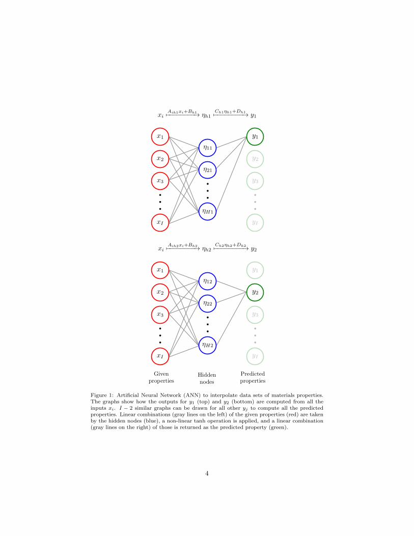
Figure 1: Artificial Neural Network (ANN) to interpolate data sets of materials properties.The graphs show how the outputs for y1 (top) and y2 (bottom) are computed from all theinputs xi. I − 2 similar graphs can be drawn for all other yj to compute all the predictedproperties. Linear combinations (gray lines on the left) of the given properties (red) are takenby the hidden nodes (blue), a non-linear tanh operation is applied, and a linear combination(gray lines on the right) of those is returned as the predicted property (green).

4

Figure 2: If we want to evaluate the ANN for a data point x which has some of the entries forits properties missing, we will follow the process described by this graph. After checking forthe trivial case where all entries are existent, we set x0 = x, and replace all the missing entriesby averages from the training data set. We then iteratively compute xn+1 as a combinationxn and f applied to xn until a certain point of convergence is reached, and return the finalxn as a result instead of f(x).

predicted property yj for 1 ≤ j ≤ I. There are exactly as many given propertiesas predicted properties, since all types of properties (defining and physical) aretreated equally by the ANN. Provided a set of parameters Aihj , Bhj , Chj , andDj , the predicted properties can be computed from the given properties. TheANN always sets Akhk = 0 for all 1 ≤ k ≤ I to ensure that the solution of thefixed-point equation is orthogonal to the identity, and so we derive a networkthat can predict yk without the knowledge of xk.

2.2. Handling incomplete data

Typically, materials data that has been obtained from experiments is in-complete, i.e. not all properties are known for every material, but the set ofmissing properties is different for each entry. However, there is informationembedded within property-property relationships: for example ultimate tensilestrength is three times hardness. A typical ANN formalism requires that eachproperty is either an input or an output of the network, and all inputs mustbe provided to obtain a valid output. In our example composition would beinputs, whereas ultimate tensile strength and hardness are outputs. To exploitthe known relationship between ultimate tensile strength and hardness, and al-low either the hardness and ultimate tensile strength to inform missing datain the other property, we treat all properties as both inputs and outputs of

5

the ANN. We have a single ANN rather than an exponentially large number ofthem (one for each combination of available composition and properties). Wethen adopt an expectation-maximization algorithm[17]. This is an iterative ap-proach, where we first provide an estimate for the missing data, and then usethe ANN to iteratively correct that initial value.

The algorithm is shown in Fig. 2. For any material x we check which proper-ties are unknown. In the non-trivial case of missing entries, we first set missingvalues to the average of the values present in the data set. An alternative ap-proach would be to adopt a value suggested by that of a local cluster. Withestimates for all values of the neural network we then iteratively compute

xn+1 = γxn + (1− γ)f(xn) . (2)

The converged result is then returned instead of f(x). The function f remainsfixed on each iteration of the cycle.

We include a softening parameter 0 ≤ γ ≤ 1. With γ = 0 we ignore theinitial guess for the unknowns in x and determine them purely by applyingf to those entries. However, introducing γ > 0 will prevent oscillations anddivergences of the sequence, typically we set γ = 0.5.

2.3. Functional properties

Many material properties are functional graphs, for example to capture thevariation of the yield stress with temperature[15]. To handle this data efficiently,we promote the two varying quantities to become interdependent vectors. Thiswill reduce the amount of memory space and computation time used by a factorroughly proportional to the number of entries in the vector quantities. It alsoallows the tool to model functional properties on the same footing as the mainmodel, rather than as a parameterization of the curve such as mean and gradient.The graph is represented by a series of points indexed by variable `. Let x bea point from a training data set. Let x1,` and x2,` be the varying graphicalproperties, and let all other properties x3, x4, . . . be normal scalar quantities.When f(x) is computed, the evaluation of the vector quantities is performedindividually for each component of the vector,

y1,l = f1(x1,`, x2,`, x3, x4, . . .) . (3)

When evaluating the scalar quantities, we aim to provide the ANN with in-formation of the x2(x1) dependency as a whole, instead of the individual datapoints (i.e. parts of the vectors x1,`, and x2,`). It is reasonable to describe thecurve in terms of different moments with respect to some basis functions formodeling the curve. For most expansions, the moment that appears in lowestorder is the average 〈x1〉, or 〈x2〉 respectively. We therefore evaluate the scalarquantities by computing,

y3 = f3(〈x1〉 , 〈x2〉 , x3, x4, . . .) . (4)

This can be extended by defining a function basis for expansion, and includetheir higher order moments. This approach automatically removes the bias dueto differeing numbers of points in the graphs.

6

2.4. Training process

The ANN has to first be trained on a provided data set. Starting fromrandom values for Aihj , Bhj , Chj , and Dj , the parameters are varied followinga random walk, and the new values are accepted, if the new function f modelsthe fixed-point equation f(x) = x better. This is quantitatively measured bythe error function,

δ =

√√√√ 1

N

∑x∈X

I∑j=1

[fj(x)− xj ]2 . (5)

The optimization proceeds by a steepest descent approach[18], where the num-ber of optimization cycles C is a run-time variable.

In order to calculate the uncertainty in the ANN’s prediction, fσ(x), we traina whole suite of ANNs simultaneously, and return their average as the overallprediction and their standard deviation as the uncertainty[19]. We choose thenumber of models M to be between 4 and 64, since this should be sufficient toextract the mean and uncertainty. In Section 3 we show how the uncertainty re-flects the noise in the training data and uncertainty in interpolation. Moreover,on systems that are not uniquely defined, knowledge of the full distribution ofmodels will expose the degenerate solutions.

2.5. Alternative approaches

ANNs like the one proposed in this paper (with one hidden layer and abounded transfer function; see Eq. (1)) can be expressed as a Gaussian processusing the construction first outlined by Neal [20] in 1996. Gaussian processeswere considered as an alternative to building the framework in this paper, butwere rejected for two reasons. Firstly, the ANNs have a lower computationalcost, which scales linearly with the number of entries N , and therefore ANNsare feasible to train and run on large-scale databases. The cost for Gaussianprocesses scales as N3, and therefore does not provide the required speed. Sec-ondly, materials data tends to be clustered. Often, experimental data is easy toproduce in one region of the parameter space, and hard to produce in anotherregion. Gaussian processes can only define a unique length-scale of correlationand consequently fail to model clustered data whereas ANNs perform well.

3. Testing and validation

Having developed the ANN formalism, we proceed by testing it on exemplardata. We will take data from a range of models to train the ANN, and validateits results. We validate the ability of the ANN to capture functional relationsbetween materials properties, handle incomplete data, and calculate graphicalquantities.

In Section 3.1, we interpolate a set of 1-dimensional functional dependencies(cosine, logarithmic, quadratic), and present a method to determine the optimalnumber of hidden nodes. In Section 3.2, we demonstrate how to determine

7

−1

−0.5

0

0.5

1

0 2 4 6 8(a)

y(x)

x

f(x) = cos(x)Gen. data

ANN

−0.5

0

0.5

1

1.5

0.5 1 1.5 2 2.5 3 3.5 4 4.5 5(b)

y(x)

x

f(x) = log(x)Gen. data

ANN

0

5

10

15

20

25

−4 −2 0 2 4(c)

y(x)

x

f(x) = x2Gen. data

ANN

0

1

2

3

4

5

6

7

1 2 3 4 5 6(d)

Uncertainty

Number of Hidden Nodes

rmsred. rmsc-v rms

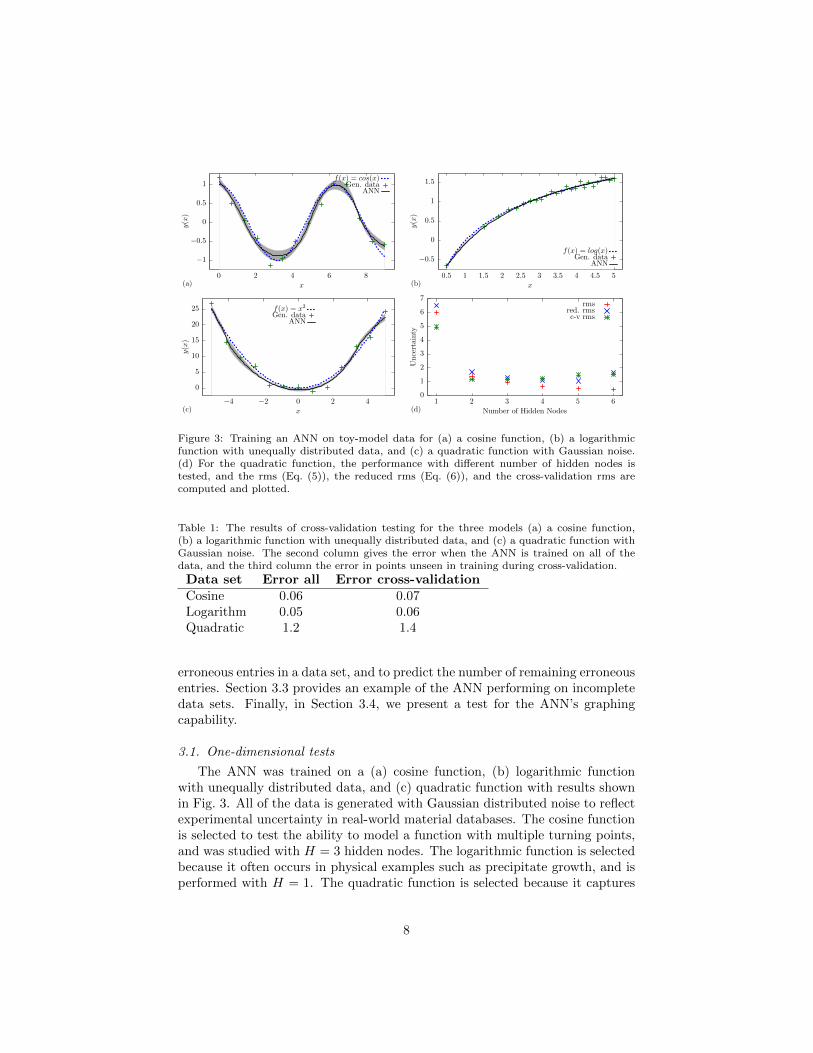
Figure 3: Training an ANN on toy-model data for (a) a cosine function, (b) a logarithmicfunction with unequally distributed data, and (c) a quadratic function with Gaussian noise.(d) For the quadratic function, the performance with different number of hidden nodes istested, and the rms (Eq. (5)), the reduced rms (Eq. (6)), and the cross-validation rms arecomputed and plotted.

Table 1: The results of cross-validation testing for the three models (a) a cosine function,(b) a logarithmic function with unequally distributed data, and (c) a quadratic function withGaussian noise. The second column gives the error when the ANN is trained on all of thedata, and the third column the error in points unseen in training during cross-validation.

Data set Error all Error cross-validationCosine 0.06 0.07Logarithm 0.05 0.06Quadratic 1.2 1.4

erroneous entries in a data set, and to predict the number of remaining erroneousentries. Section 3.3 provides an example of the ANN performing on incompletedata sets. Finally, in Section 3.4, we present a test for the ANN’s graphingcapability.

3.1. One-dimensional tests

The ANN was trained on a (a) cosine function, (b) logarithmic functionwith unequally distributed data, and (c) quadratic function with results shownin Fig. 3. All of the data is generated with Gaussian distributed noise to reflectexperimental uncertainty in real-world material databases. The cosine functionis selected to test the ability to model a function with multiple turning points,and was studied with H = 3 hidden nodes. The logarithmic function is selectedbecause it often occurs in physical examples such as precipitate growth, and isperformed with H = 1. The quadratic function is selected because it captures

8

the two lowest term in a Taylor expansion, and is performed with H = 2.Fig. 3 shows that the ANN recovers the underlying functional dependence

of the data sets well. The uncertainty of the model is larger at the boundaries,because the ANN has less information about the gradient. The uncertaintyalso reflects the Gaussian noise in the training data, as can be observed fromthe test with the log function, where we increased the Gaussian noise of thegenerated data from left to right in this test. For the test on the sin function,the ANN has a larger uncertainty for maxima and minima, because these havehigher curvature, and are therefore harder to fit. The correct modeling of thesmooth curvature of the cosine curve could not be captured by simple linearinterpolation.

The choice of the number of hidden nodes H is critical: Too few will preventthe ANN from modeling the data accurately; too many hidden nodes leads toover-fitting. To study the effect of changing the number of hidden nodes, werepeat the training process for the quadratic function with 1 ≤ H ≤ 6, anddetermine the error δ in three ways. Firstly, the straight error δ. The secondapproach is cross-validation by comparing to additional unseen data[21]. Thethird and final approach is evaluate the reduced error

δ∗ =δ√

1− 2H/N, (6)

which assumes that the sum of the squares in Eq. (5) is χ2-distributed, sowe calculate the error per degree of freedom, which is N − 2H, where the 2Hparameters in the ANN arise because each of the H indicator functions in Eq. (1)has two degrees of freedom: a scaling factor and also a shift. The results arepresented in Fig. 3(d).

The error, δ, monotonically falls with more hidden nodes. This is expectedas more hidden nodes gives the model the flexibility to describe the trainingdata more accurately. However, it is important that the ANN models the un-derlying functional dependence between those data points well, and does notintroduce overfitting. The cross-validation results increase above H = 2 hiddennodes, which implies that overfitting is induced beyond this point. Therefore,H = 2 is the optimal number of hidden nodes for the quadratic test. This is ex-pected since we choose tanh as the basis functions to build our ANN, which is amonotonic function, and the quadratic consists of two parts that are decreasingand increasing respectively.

In theory, performing a cross-validation test may provide more insight intothe performance of the ANN on a given data set, however, this is usually notpossible because it has a high computational cost. We therefore turn to thereduced error, δ∗. This also has a minimum at H = 2, and represents a quickand robust approach to determine the optimal number of hidden nodes.

Cross-validation also provides an approach to confirm the accuracy of theANN predictions. For the optimal number of hidden nodes we perform a cross-validation analysis by taking the three examples in Fig. 3, remove one quarterof the points at random, train a model on the remaining three quarters of

9

−10

0

10

20

30

0 1 2 3 4 5

y(x)

x

Toy modelGood entriesBad entries

ANN

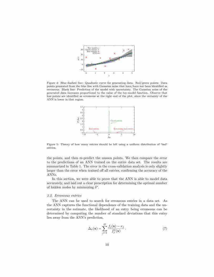
Figure 4: Blue dashed line: Quadratic curve for generating data. Red/green points: Datapoints generated from the blue line with Gaussian noise that have/have not been identified aserroneous. Black line: Prediction of the model with uncertainty. The Gaussian noise of thegenerated data increases proportional to the value of the toy-model function. Observe thatless points are identified as erroneous at the right end of the plot, since the certainty of theANN is lower in that region.

0

0.5

1

1.5

2

2.5

3

3.5

4

4.5

−10 −5 0 5 10

Good entries

Bad entries Remaining bad entries

P(∆

y)

∆y

Figure 5: Theory of how many entries should be left using a uniform distribution of ’bad’entries.

the points, and then re-predict the unseen points. We then compare the errorto the predictions of an ANN trained on the entire data set. The results aresummarized in Table 1. The error in the cross-validation analysis is only slightlylarger than the error when trained off all entries, confirming the accuracy of theANNs.

In this section, we were able to prove that the ANN is able to model dataaccurately, and laid out a clear prescription for determining the optimal numberof hidden nodes by minimizing δ∗.

3.2. Erroneous entries

The ANN can be used to search for erroneous entries in a data set. Asthe ANN captures the functional dependence of the training data and the un-certainty in the estimate, the likelihood of an entry being erroneous can bedetermined by computing the number of standard deviations that this entrylies away from the ANN’s prediction,

∆σ(x) =

G∑j=1

fj(x)− xjfσj (x)

. (7)

10

0

10

20

30

40

5 10 15 20 25 30 35 40

Erron

eousentriesremaining

Erroneous entries removed

TruePredicted

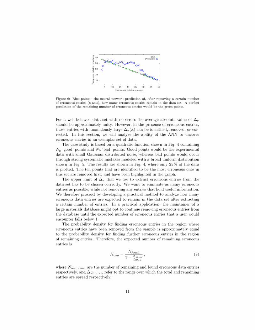
Figure 6: Blue points: the neural network prediction of, after removing a certain numberof erroneous entries (x-axis), how many erroneous entries remain in the data set. A perfectprediction of the remaining number of erroneous entries would be the green points.

For a well-behaved data set with no errors the average absolute value of ∆σ

should be approximately unity. However, in the presence of erroneous entries,those entries with anomalously large ∆σ(x) can be identified, removed, or cor-rected. In this section, we will analyze the ability of the ANN to uncovererroneous entries in an exemplar set of data.

The case study is based on a quadratic function shown in Fig. 4 containingNg ‘good’ points and Nb ‘bad’ points. Good points would be the experimentaldata with small Gaussian distributed noise, whereas bad points would occurthrough strong systematic mistakes modeled with a broad uniform distributionshown in Fig. 5. The results are shown in Fig. 4, where only 25 % of the datais plotted. The ten points that are identified to be the most erroneous ones inthis set are removed first, and have been highlighted in the graph.

The upper limit of ∆σ that we use to extract erroneous entries from thedata set has to be chosen correctly. We want to eliminate as many erroneousentries as possible, while not removing any entries that hold useful information.We therefore proceed by developing a practical method to analyze how manyerroneous data entries are expected to remain in the data set after extractinga certain number of entries. In a practical application, the maintainer of alarge materials database might opt to continue removing erroneous entries fromthe database until the expected number of erroneous entries that a user wouldencounter falls below 1.

The probability density for finding erroneous entries in the region whereerroneous entries have been removed from the sample is approximately equalto the probability density for finding further erroneous entries in the regionof remaining entries. Therefore, the expected number of remaining erroneousentries is

Nrem =Nfound

1− ∆yrem∆ytot

, (8)

where Nrem,found are the number of remaining and found erroneous data entriesrespectively, and ∆ytot,rem refer to the range over which the total and remainingentries are spread respectively.

11

0

2

4

6

8

10

12

0 2 4 6 8 10

z(x)

x

Training dataPred z w/o xPred z w/o y

Figure 7: The toy-model data that is used for training of the ANN is shown as Z as a functionof X together with the predictions of the ANN without providing X or Y respectively. TheANN learns the Z = X + Y dependence, and uses the average of X or Y values respectivelyto replace the unknown values.

Returning to the exemplar data set, we compare Nrem with the true numberof remaining erroneous entries in Fig. 6. The method provides a good predictionfor the actual number of remaining erroneous entries.

The neural network can identify the erroneous entries in a data set. Fur-thermore, the tool can predict which are the entries most likely to be erroneousallowing the end user to prioritize their attention on the worse entries. Thecapability to predict the remaining number of entries allows the end user tosearch through and correct erroneous entries until a target quality threshold isattained.

3.3. Incomplete data

In the following section, we investigate the capability of the ANN to trainon and analyze incomplete data. This requires at least three different propertiesto study, and therefore our tests will be on three-dimensional data sets. Thisprocedure can be studied for different levels of correlation between the proper-ties, and we study two limiting classes: completely uncorrelated, and completelycorrelated data. In the uncorrelated data set the two input variables are uncor-related with each other, but still correlated to the output. In the correlated dataset the input variables are now correlated with each other, and also correlatedto the output. We focus first on the uncorrelated data.

3.3.1. Fully uncorrelated data

To study the performance on uncorrelated data we perform the followingtwo independent tests: we first train the ANN on incomplete uncorrelated data,and run it on complete data, and secondly train on complete uncorrelated data,and run on incomplete data.

For N = 20 points X = {x1, . . . , xN} distributed evenly in the interval0 ≤ x ≤ 10 we generate a set of random numbers Y = (y1, . . . , yN ) uniformlydistributed between −2.5 to 2.5. We let Z = X + Y = (x1 + y1, . . . , xN + zN ),which is shown in Fig. 7. This data set is uncorrelated because the values of Y ,a set of random numbers, are independent of the values X; therefore a modelneeds both x and y to calculate z.

12

−0.6

−0.4

−0.2

0

0.2

0.4

0.6

0 2 4 6 8 10

∆z(x

)x

Exact0% frag

40% frag50% frag

60% frag

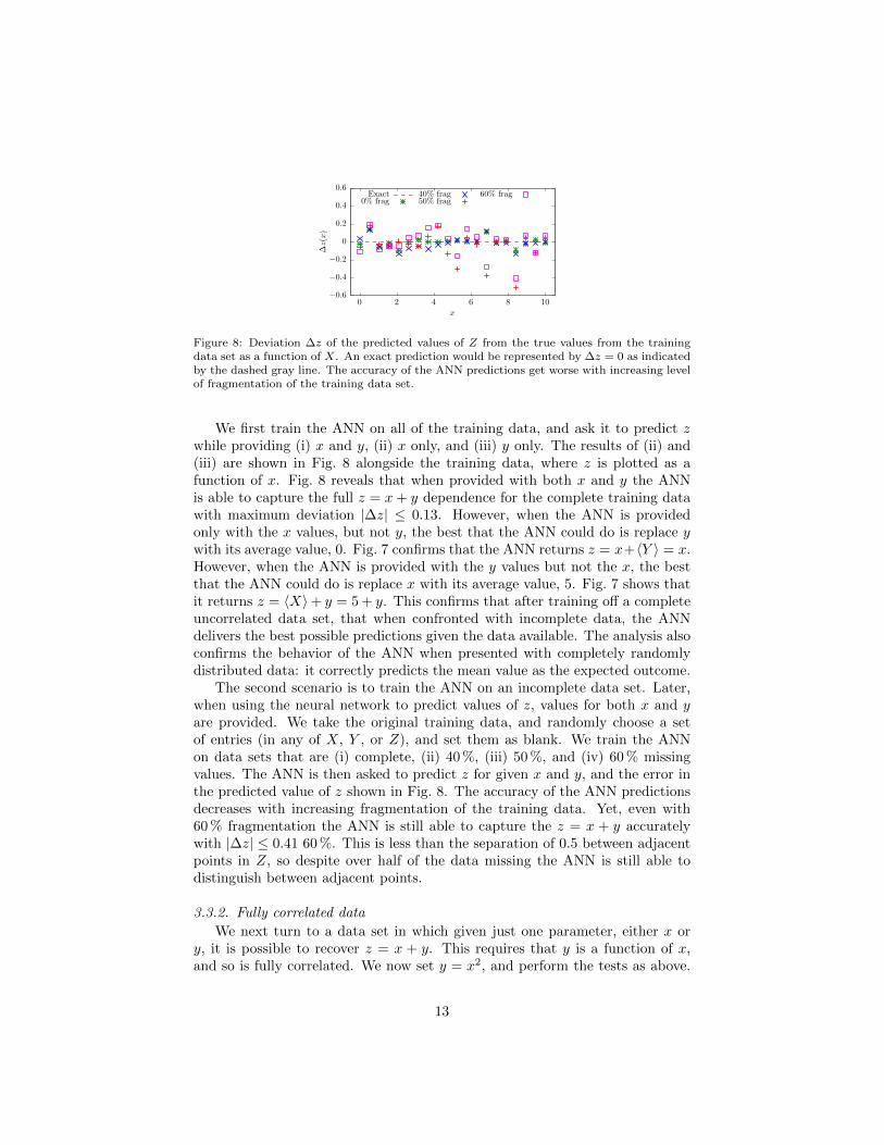
Figure 8: Deviation ∆z of the predicted values of Z from the true values from the trainingdata set as a function of X. An exact prediction would be represented by ∆z = 0 as indicatedby the dashed gray line. The accuracy of the ANN predictions get worse with increasing levelof fragmentation of the training data set.

We first train the ANN on all of the training data, and ask it to predict zwhile providing (i) x and y, (ii) x only, and (iii) y only. The results of (ii) and(iii) are shown in Fig. 8 alongside the training data, where z is plotted as afunction of x. Fig. 8 reveals that when provided with both x and y the ANNis able to capture the full z = x+ y dependence for the complete training datawith maximum deviation |∆z| ≤ 0.13. However, when the ANN is providedonly with the x values, but not y, the best that the ANN could do is replace ywith its average value, 0. Fig. 7 confirms that the ANN returns z = x+〈Y 〉 = x.However, when the ANN is provided with the y values but not the x, the bestthat the ANN could do is replace x with its average value, 5. Fig. 7 shows thatit returns z = 〈X〉+ y = 5 + y. This confirms that after training off a completeuncorrelated data set, that when confronted with incomplete data, the ANNdelivers the best possible predictions given the data available. The analysis alsoconfirms the behavior of the ANN when presented with completely randomlydistributed data: it correctly predicts the mean value as the expected outcome.

The second scenario is to train the ANN on an incomplete data set. Later,when using the neural network to predict values of z, values for both x and yare provided. We take the original training data, and randomly choose a setof entries (in any of X, Y , or Z), and set them as blank. We train the ANNon data sets that are (i) complete, (ii) 40 %, (iii) 50 %, and (iv) 60 % missingvalues. The ANN is then asked to predict z for given x and y, and the error inthe predicted value of z shown in Fig. 8. The accuracy of the ANN predictionsdecreases with increasing fragmentation of the training data. Yet, even with60 % fragmentation the ANN is still able to capture the z = x + y accuratelywith |∆z| ≤ 0.41 60 %. This is less than the separation of 0.5 between adjacentpoints in Z, so despite over half of the data missing the ANN is still able todistinguish between adjacent points.

3.3.2. Fully correlated data

We next turn to a data set in which given just one parameter, either x ory, it is possible to recover z = x + y. This requires that y is a function of x,and so is fully correlated. We now set y = x2, and perform the tests as above.

13

5

10

15

20

25

30

35

40

45

50

0 2 4 6 8 10

z(x,y)

y

ModelGen. data

ANN

x = 1

x = 5

Figure 9: Training data, true function and predicted ANN function for different values of x.

1

2

3

4

5

2 3 4 5 6 7 8 9 10

Prediction

forx

Number of provided entries

Figure 10: Predict x from the training data with different number of (y, z)- pairs provided.The gray dotted lines indicate the true value of x.

Now after training on a complete data set, the ANN is able to predict valuesfor z when given only x or y. The ANN also performs well when trained froman incomplete data set.

3.3.3. Summary

We have successfully tested the capability of the ANN to handle incompletedata sets. We performed tests for both training and running the ANN withincomplete data. The ANN performs well when the training data is both fullycorrelated and completely uncorrelated, so should work well on real-life data.

3.4. Functional properties

We now test the capability for the ANN to handle data with functionalproperties (also referred to as graphing data) as a single entity. As before wehave a functional variable X = {x1, . . . , xN} with N = 5 equidistant pointsin the interval from 1 to 5. At each value of x point we introduce a vectorquantity, dependent on a variable Y = {y1, . . . , y`} that can have up to ` = 10.We compute the vector function z` = 4x+ y2

`/4, with additional Gaussian noiseof width 1 and train an ANN on this data set. We show the training data aswell as the ANN prediction for z in Fig. 9, which confirms that the ANN is ableto predict the underlying functional dependence correctly.

The real power of the graphing capability is to predict x with different num-ber of elements provided in the vector (y, z). We show the predictions of theANN in Fig. 10. With all 10 components of the vector provided the ANN makes

14

accurate predictions for x. With fewer components provided the accuracy of thepredictions for x falls, but even if just 2 elements are provided the ANN is stillable to distinguish between the discrete values of x.

We confirm that the ANN is able to fully handle vector and graphical data.The ANN gives accurate predictions for both the functional properties whenproviding non-functional properties only, and vice-versa. This new capabilityallows the ANN to handle a new form of real-world problems, for example thetemperature dependence of variables such as yield stress. Temperature can beused only as an input for the yield stress, without the need to replicate otherproperties that are not temperature dependent, for example cost. The reductionin the amount of data required will increase the efficiency of the approach andtherefore the quality of the predictions.

4. Applications

With the testing on model data complete we now present case studies of ap-plying the ANN to real-life data. In this section, we will use the ANN frameworkto analyze the MaterialUniverse and Prospector Plastics databases. We first fo-cus on a data set of 1641 metal alloys with a composition space of 31 dimensions(that is each metal is an alloy of potentially 31 chemical elements). We trainneural networks of 4 hidden nodes to predict properties such as the density, themelting point temperature, the yield stress, and the fracture toughness of thosematerials. Secondly, we examine a system where not all compositional variablesare available: a polymer data set of 5656 entries, and focus on the modeling ofits tensile modulus.

We use the trained ANN to uncover errors by searching for entries multi-ple standard deviations ∆σ away from the ANN predictions. We compare theresults to primary sources referenced from the MaterialUniverse data set to de-termine whether the entry was actually erroneous: a difference could only be dueto a transcription error from that primary data set into the MaterialUniversedatabase.

When analyzing the density data, we can confirm the ability of the ANNto identify erroneous entries with a fidelity of over 50 %. For the melting tem-perature data, we show that for missing entries the ANN yields a significantimprovement in the estimates provided by the curators of the database. Whenadvancing to the yield stress properties of the materials, we observe that ourmethods can only be applied when additional heat treatment data is madeavailable for training the ANN. Unlike established methods, our framework isuniquely positioned to include such data for error-finding and extrapolation. Forthe fracture toughness data, we exploit correlations with other known proper-ties to provide more accurate estimation functions compared to established ones.Finally, in the polymer data, we exploit the capability of our ANN to handle anincomplete data set without compositional variables, and instead characterizepolymers by their properties.

15

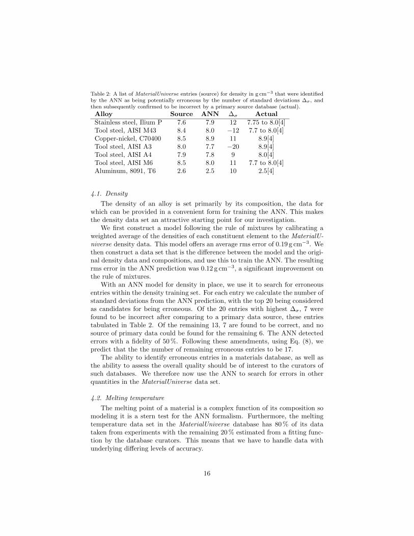
Table 2: A list of MaterialUniverse entries (source) for density in g cm−3 that were identifiedby the ANN as being potentially erroneous by the number of standard deviations ∆σ , andthen subsequently confirmed to be incorrect by a primary source database (actual).

Alloy Source ANN ∆σ ActualStainless steel, Ilium P 7.6 7.9 12 7.75 to 8.0[4]Tool steel, AISI M43 8.4 8.0 −12 7.7 to 8.0[4]Copper-nickel, C70400 8.5 8.9 11 8.9[4]Tool steel, AISI A3 8.0 7.7 −20 8.9[4]Tool steel, AISI A4 7.9 7.8 9 8.0[4]Tool steel, AISI M6 8.5 8.0 11 7.7 to 8.0[4]Aluminum, 8091, T6 2.6 2.5 10 2.5[4]

4.1. Density

The density of an alloy is set primarily by its composition, the data forwhich can be provided in a convenient form for training the ANN. This makesthe density data set an attractive starting point for our investigation.

We first construct a model following the rule of mixtures by calibrating aweighted average of the densities of each constituent element to the MaterialU-niverse density data. This model offers an average rms error of 0.19 g cm−3. Wethen construct a data set that is the difference between the model and the origi-nal density data and compositions, and use this to train the ANN. The resultingrms error in the ANN prediction was 0.12 g cm−3, a significant improvement onthe rule of mixtures.

With an ANN model for density in place, we use it to search for erroneousentries within the density training set. For each entry we calculate the number ofstandard deviations from the ANN prediction, with the top 20 being consideredas candidates for being erroneous. Of the 20 entries with highest ∆σ, 7 werefound to be incorrect after comparing to a primary data source, these entriestabulated in Table 2. Of the remaining 13, 7 are found to be correct, and nosource of primary data could be found for the remaining 6. The ANN detectederrors with a fidelity of 50 %. Following these amendments, using Eq. (8), wepredict that the the number of remaining erroneous entries to be 17.

The ability to identify erroneous entries in a materials database, as well asthe ability to assess the overall quality should be of interest to the curators ofsuch databases. We therefore now use the ANN to search for errors in otherquantities in the MaterialUniverse data set.

4.2. Melting temperature

The melting point of a material is a complex function of its composition somodeling it is a stern test for the ANN formalism. Furthermore, the meltingtemperature data set in the MaterialUniverse database has 80 % of its datataken from experiments with the remaining 20 % estimated from a fitting func-tion by the database curators. This means that we have to handle data withunderlying differing levels of accuracy.

16

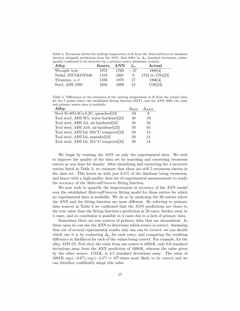
Table 3: Erroneous entries for melting temperature in K from the MaterialUniverse database(source) alongside predictions from the ANN, that differ by ∆σ standard deviations, subse-quently confirmed to be incorrect by a primary source databases (actual).

Alloy Source ANN ∆σ ActualWrought iron 1973 1760 −37 1808[4]Nickel, INCOLOY840 1419 1661 8 1724 to 1784[22]Titanium, α-β 1593 1878 17 1866[4]Steel, AISI 1095 1650 1699 13 1788[23]

Table 4: Differences in the estimates of the melting temperature in K from the actual valuefor the 7 points where the established fitting function (EFF), and the ANN differ the mostand primary source data is available.

Alloy ∆EFF ∆ANN

Steel Fe-9Ni-4Co-0.2C, quenched[24] -94 9Tool steel, AISI W5, water-hardened[24] 48 -19Tool steel, AISI A4, air-hardened[24] 56 16Tool steel, AISI A10, air-hardened[23] 59 -61Tool steel, AISI L6, 650 ◦C tempered[24] 59 14Tool steel, AISI L6, annealed[24] 59 14Tool steel, AISI L6, 315 ◦C tempered[24] 59 14

We begin by training the ANN on only the experimental data. We seekto improve the quality of the data set by searching and correcting erroneousentries as was done for density. After identifying and correcting the 4 incorrectentries listed in Table 3, we estimate that there are still 5 erroneous entries inthe data set. This leaves us with just 0.3 % of the database being erroneous,and hence with a high-quality data set of experimental measurements to studythe accuracy of the MaterialUniverse fitting function.

We now wish to quantify the improvement in accuracy of the ANN modelover the established MaterialUniverse fitting model for those entries for whichno experimental data is available. We do so by analyzing the 30 entries wherethe ANN and the fitting function are most different. By referring to primarydata sources in Table 4 we confirmed that the ANN predictions are closer tothe true value than the fitting function’s prediction in 20 cases, further away in4 cases, and no conclusion is possible in 4 cases due to a lack of primary data.

Sometimes there are two sources of primary data that are inconsistent. Inthese cases we can use the ANN to determine which source is correct. Assumingthat out of several experimental results only one can be correct, we can decidewhich one it is by evaluating ∆σ for each entry, and comparing the resultingdifference in likelihood for each of the values being correct. For example, for thealloy AISI O1 Tool steel, the value from one source is 1694 K, only 0.6 standarddeviations away from the ANN prediction of 1698 K, whereas the value givenby the other source, 1723 K, is 4.5 standard deviations away. The value of1694 K exp (−0.62)/ exp (−4.52) ≈ 109-times more likely to be correct and wecan therefore confidently adopt this value.

17

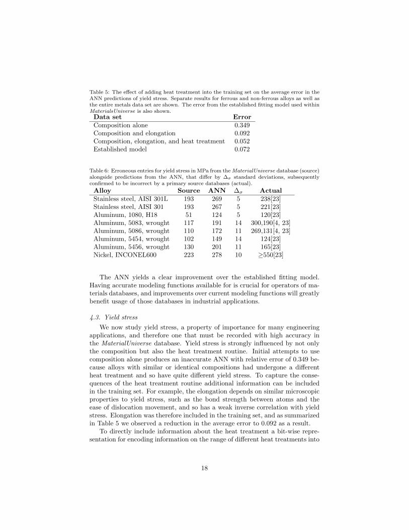
Table 5: The effect of adding heat treatment into the training set on the average error in theANN predictions of yield stress. Separate results for ferrous and non-ferrous alloys as well asthe entire metals data set are shown. The error from the established fitting model used withinMaterialsUniverse is also shown.Data set ErrorComposition alone 0.349Composition and elongation 0.092Composition, elongation, and heat treatment 0.052Established model 0.072

Table 6: Erroneous entries for yield stress in MPa from the MaterialUniverse database (source)alongside predictions from the ANN, that differ by ∆σ standard deviations, subsequentlyconfirmed to be incorrect by a primary source databases (actual).

Alloy Source ANN ∆σ ActualStainless steel, AISI 301L 193 269 5 238[23]Stainless steel, AISI 301 193 267 5 221[23]Aluminum, 1080, H18 51 124 5 120[23]Aluminum, 5083, wrought 117 191 14 300,190[4, 23]Aluminum, 5086, wrought 110 172 11 269,131[4, 23]Aluminum, 5454, wrought 102 149 14 124[23]Aluminum, 5456, wrought 130 201 11 165[23]Nickel, INCONEL600 223 278 10 ≥550[23]

The ANN yields a clear improvement over the established fitting model.Having accurate modeling functions available for is crucial for operators of ma-terials databases, and improvements over current modeling functions will greatlybenefit usage of those databases in industrial applications.

4.3. Yield stress

We now study yield stress, a property of importance for many engineeringapplications, and therefore one that must be recorded with high accuracy inthe MaterialUniverse database. Yield stress is strongly influenced by not onlythe composition but also the heat treatment routine. Initial attempts to usecomposition alone produces an inaccurate ANN with relative error of 0.349 be-cause alloys with similar or identical compositions had undergone a differentheat treatment and so have quite different yield stress. To capture the conse-quences of the heat treatment routine additional information can be includedin the training set. For example, the elongation depends on similar microscopicproperties to yield stress, such as the bond strength between atoms and theease of dislocation movement, and so has a weak inverse correlation with yieldstress. Elongation was therefore included in the training set, and as summarizedin Table 5 we observed a reduction in the average error to 0.092 as a result.

To directly include information about the heat treatment a bit-wise repre-sentation for encoding information on the range of different heat treatments into

18

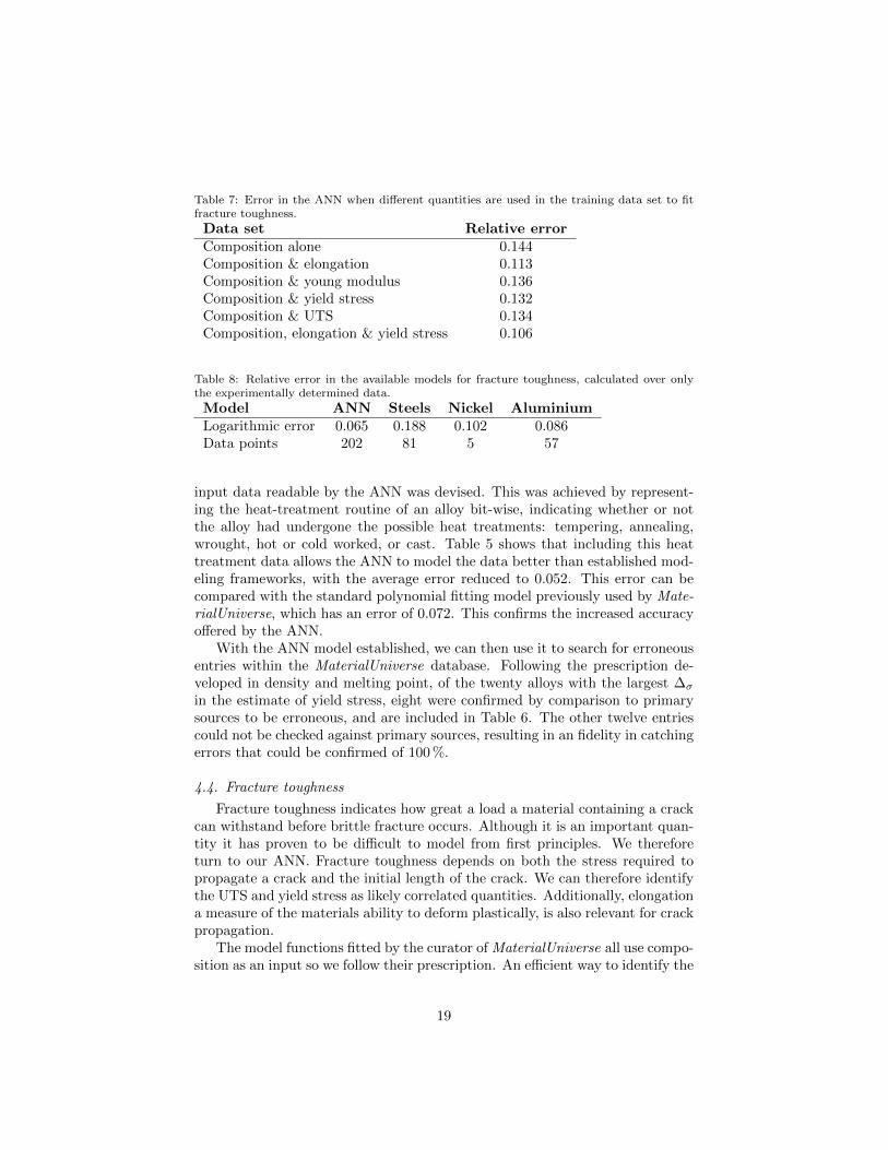
Table 7: Error in the ANN when different quantities are used in the training data set to fitfracture toughness.

Data set Relative errorComposition alone 0.144Composition & elongation 0.113Composition & young modulus 0.136Composition & yield stress 0.132Composition & UTS 0.134Composition, elongation & yield stress 0.106

Table 8: Relative error in the available models for fracture toughness, calculated over onlythe experimentally determined data.

Model ANN Steels Nickel AluminiumLogarithmic error 0.065 0.188 0.102 0.086Data points 202 81 5 57

input data readable by the ANN was devised. This was achieved by represent-ing the heat-treatment routine of an alloy bit-wise, indicating whether or notthe alloy had undergone the possible heat treatments: tempering, annealing,wrought, hot or cold worked, or cast. Table 5 shows that including this heattreatment data allows the ANN to model the data better than established mod-eling frameworks, with the average error reduced to 0.052. This error can becompared with the standard polynomial fitting model previously used by Mate-rialUniverse, which has an error of 0.072. This confirms the increased accuracyoffered by the ANN.

With the ANN model established, we can then use it to search for erroneousentries within the MaterialUniverse database. Following the prescription de-veloped in density and melting point, of the twenty alloys with the largest ∆σ

in the estimate of yield stress, eight were confirmed by comparison to primarysources to be erroneous, and are included in Table 6. The other twelve entriescould not be checked against primary sources, resulting in an fidelity in catchingerrors that could be confirmed of 100 %.

4.4. Fracture toughness

Fracture toughness indicates how great a load a material containing a crackcan withstand before brittle fracture occurs. Although it is an important quan-tity it has proven to be difficult to model from first principles. We thereforeturn to our ANN. Fracture toughness depends on both the stress required topropagate a crack and the initial length of the crack. We can therefore identifythe UTS and yield stress as likely correlated quantities. Additionally, elongationa measure of the materials ability to deform plastically, is also relevant for crackpropagation.

The model functions fitted by the curator of MaterialUniverse all use compo-sition as an input so we follow their prescription. An efficient way to identify the

19

0

1000

2000

3000

4000

5000

6000

7000

8000

0.8 0.9 1 1.1 1.2 1.3 1.4

Ten

sile

Modu

lus

inM

Pa

Density in g/cm

Glass fibre fillerMineral filler

Unkn./zero filler

Figure 11: Polymer tensile modulus against density with glass fiber filler (blue) and mineralfiller (red). The input information includes not only the filler type but also the filler amount(weight in %).

properties most strongly correlated to fracture toughness is to train the ANNwith each quantity in turn (in addition to the composition data), and then eval-uate the deviation from the fracture toughness data. The properties for whichthe error is minimized are the most correlated. Table 7 shows that elongationis the property most strongly correlated to fracture toughness. Whilst yieldstress, Young modulus, and UTS offer some reduction in the error, includingthese quantities to the training data will not lead to a significant improvementon the average error obtained from composition and elongation alone.

The MaterialUniverse fracture toughness data contains only around 200 val-ues that have been determined experimentally, with the remaining 1400 valuesestimated by fitting functions. These are polynomial functions which take com-position and elongation as input, and are fitted to either steels, nickel, or alu-minum separately. We train the ANN over just the experimentally determineddata, and compare the error in its predictions to those from the known fittingfunctions. Table 8 shows that the ANN is the most accurate, having a smallererror than the fitting function for all three alloy families. While the differentfitting functions are ‘trained’ only on the subset of the data for which they aredesigned, the ANN is able to use information gathered from the entire data setto produce a better model over each individual subset. This is one of the keyadvantages of a ANN over traditional data modeling methods.

4.5. Polymers

In this section, we study polymers, which is an incomplete data set. Polymercomposition cannot be described simply by percentage of constituent elements(as in the previous example with metals) due to the complexity of chemicalbonding, so we must characterize the polymers by their properties. Some prop-erties are physical, such as tensile modulus and density; others take discretevalues, such as type of polymer or filler used, and filler percentage. As thedata [6] was originally compiled from manufacturer’s data sheets, not all entriesfor these properties are known, rendering the data set incomplete.

We analyze a database of polymers that has the filler type as a class-separableproperty. Many other properties exhibit a split based on filler type, such as

20

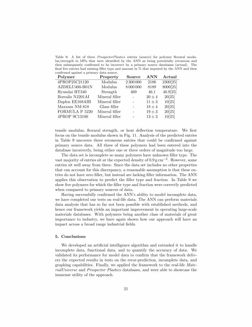
Table 9: A list of three ProspectorPlastics entries (source) for polymer flexural modu-lus/strength in MPa that were identified by the ANN as being potentially erroneous andthen subsequently confirmed to be incorrect by a primary source databases (actual). Thefinal five entries had missing filler type and amount in % that imputed by the ANN and thenconfirmed against a primary data source.

Polymer Property Source ANN Actual4PROP25C21120 Modulus 2 300 000 2186 2300[25]AZDELU400-B01N Modulus 8 000 000 8189 8000[25]Hyundai HT340 Strength 469 46.1 46.9[25]Borealis NJ201AI Mineral filler - 20± 4 20[25]Daplen EE168AIB Mineral filler - 11± 3 10[25]Maxxam NM-818 Glass filler - 18± 4 20[25]FORMULA P 5220 Mineral filler - 19± 3 20[25]4PROP 9C13100 Mineral filler - 13± 3 10[25]

tensile modulus, flexural strength, or heat deflection temperature. We firstfocus on the tensile modulus shown in Fig. 11. Analysis of the predicted entriesin Table 9 uncovers three erroneous entries that could be confirmed againstprimary source data. All three of these polymers had been entered into thedatabase incorrectly, being either one or three orders of magnitude too large.

The data set is incomplete so many polymers have unknown filler type. Thevast majority of entries sit at the expected density of 0.9 g cm−3. However, someentries sit well away from there. Since the data set includes no other propertiesthat can account for this discrepancy, a reasonable assumption is that these en-tries do not have zero filler, but instead are lacking filler information. The ANNapplies this observation to predict the filler type and fraction. In Table 9 weshow five polymers for which the filler type and fraction were correctly predictedwhen compared to primary sources of data.

Having successfully confirmed the ANN’s ability to model incomplete data,we have completed our tests on real-life data. The ANN can perform materialsdata analysis that has so far not been possible with established methods, andhence our framework yields an important improvement in operating large-scalematerials databases. With polymers being another class of materials of greatimportance to industry, we have again shown how our approach will have animpact across a broad range industrial fields.

5. Conclusions

We developed an artificial intelligence algorithm and extended it to handleincomplete data, functional data, and to quantify the accuracy of data. Wevalidated its performance for model data to confirm that the framework deliv-ers the expected results in tests on the error-prediction, incomplete data, andgraphing capabilities. Finally, we applied the framework to the real-life Mate-rialUniverse and Prospector Plastics databases, and were able to showcase theimmense utility of the approach.

21

In particular, we were able to propose and verify erroneous entries, provideimprovements in extrapolations to give estimates for unknowns, impute missingdata on materials composition and fabrication, and also help the characteriza-tion of materials by identifying non-obvious descriptors across a broad range ofdifferent applications. Therefore, we were able to show how artificial intelligencealgorithms can contribute significantly to innovation in researching, designing,and selecting materials for industrial applications.

The authors thank Bryce Conduit, Patrick Coulter, Richard Gibbens, Al-fred Ireland, Victor Kouzmanov, Hauke Neitzel, Diego Oliveira Sanchez, andHoward Stone for useful discussions, and acknowledge the financial support ofthe EPSRC [EP/J017639/1] and the Royal Society. There is Open Access tothis paper and data available at https://www.openaccess.cam.ac.uk.

[1] M. Ashby, Materials Selection in Mechanical Design, Butterworth-Heinemann, 2004.

[2] A. Jain, S. P. Ong, G. Hautier, W. Chen, W. D. Richards,S. Dacek, S. Cholia, D. Gunter, D. Skinner, G. Ceder,K. a. Persson, APL Materials 1 (2013) 011002. URL:http://link.aip.org/link/AMPADS/v1/i1/p011002/s1&Agg=doi.doi:10.1063/1.4812323.

[3] NoMaD, http://nomad-repository.eu/, 2017.

[4] MatWeb, LLC, http://www.matweb.com/, 2017.

[5] Granta Design, MaterialUniverse, CES EduPack 2017,https://www.grantadesign.com/products/data/materialuniverse.htm,2017.

[6] Granta Design, Prospector Plastics, CES EduPack 2017,https://www.grantadesign.com/products/data/ul.htm, 2017.

[7] S. Zhang, L. Li, A. Kumar, Materials Characterization Techniques, CRC,2008.

[8] E. Tadmor, R. Miller, Modeling Materials: Continuum, Atomistic and Mul-tiscale Techniques, Cambridge University Press, 2011.

[9] B. Conduit, N. Jones, H. Stone, G. Conduit, Materials & Design 131 (2017)358.

[10] B. Conduit, G. Conduit, H. Stone, M. Hardy, Development of a new nickelbased superalloy for a combustor liner and other high temperature appli-cations, Patent GB1408536, 2014.

[11] B. Conduit, G. Conduit, H. Stone, M. Hardy, Molybdenum-niobium alloysfor high temperature applications, Patent GB1307535.3, 2013.

22

[12] B. Conduit, G. Conduit, H. Stone, M. Hardy, Molybdenum-hafnium alloysfor high temperature applications, Patent EP14161255, US 2014/223465,2014.

[13] B. Conduit, G. Conduit, H. Stone, M. Hardy, Molybdenum-niobium alloysfor high temperature applications, Patent EP14161529, US 2014/224885,2014.

[14] B. Conduit, G. Conduit, H. Stone, M. Hardy, A nickel alloy, PatentEP14157622, amendment to US 2013/0052077 A2, 2014.

[15] R. Ritchie, J. Knott, J. Me. Phys. Solids 21 (1973) 395–410.

[16] O. Oliveira Jr., J. Rodrigues Jr., M. de Oliveira, Neural Networks (2016).

[17] T. Krishnan, G. McLachlan, The EM Algorithm and Extensions, Wiley,2008.

[18] C. Floudas, P. Pardalos, Encyclopedia of Optimization, Springer, 2008.

[19] H. Steck, T. Jaakkola, in: Advances in Neural Information Processing Sys-tems 16: Proceedings of the 2003 Conference, p. 521.

[20] R. Neal, Bayesian learning for neural networks, Lecture notes in statistics; 118, Springer, New York, 1996.

[21] T. Hill, P. Lewicki, Statistics: Methods and Applications, StatSoft, 2005.

[22] Longhai Special Steel Co., Ltd, China steel suppliers,http://www.steelgr.com/Steel-Grades/High-Alloy/incoloy-alloy-840.html,2017.

[23] AZoM, https://www.azom.com/, 2017.

[24] Metal Suppliers Online, LLS, www.metalsuppliersonline.com/, 2017.

[25] PolyOne, http://www.polyone.com/resources/technical-data-sheets/,2017.

23