Math 116 Calculus II

Contents

5 Exponential and Logarithmic functions 2

5.1 Review . . . . . . . . . . . . . . . . . . . . . . . . . . . . . . . . . . . . . . . . . . . 2

5.1.1 Exponential functions . . . . . . . . . . . . . . . . . . . . . . . . . . . . . . . 2

5.1.2 Logarithmic functions . . . . . . . . . . . . . . . . . . . . . . . . . . . . . . . 3

5.1.3 Relation between Exp and Log functions . . . . . . . . . . . . . . . . . . . . . 4

6 Integration 5

6.1 Antiderivatives and the Rules of integration . . . . . . . . . . . . . . . . . . . . . . . . 5

6.2 Integration by Substitution . . . . . . . . . . . . . . . . . . . . . . . . . . . . . . . . . 7

6.3 Area and the definite integral . . . . . . . . . . . . . . . . . . . . . . . . . . . . . . . . 9

6.4 The fundamental theorem of Calculus . . . . . . . . . . . . . . . . . . . . . . . . . . . 15

6.5 Evaluating definite integrals . . . . . . . . . . . . . . . . . . . . . . . . . . . . . . . . 17

6.6 Area between two curves . . . . . . . . . . . . . . . . . . . . . . . . . . . . . . . . . . 19

6.7 Applications of the Definite integral to Business and Economics . . . . . . . . . . . . . 23

1

Chapter 5

Exponential and Logarithmic functions

5.1 Review

5.1.1 Exponential functions

Definition:

• e = 2.7182818.

• f(x) = ex.

Properties:

• domain: (−∞,∞).

• Range: (0,+∞).

• f(0) = 1.

• Continuous.

• increasing.

Laws of exponents:

• ex ∗ ey = ex+y;

• ex

ey= ex−y;

2

• (ex)y = exy;

Differentiation:

• d

dxex = ex;

• d

dxef(x) = ef(x) ∗ f ′(x);

Example 1 Calculate e−10, e−2, e0,e1, e10 using calculator.

Example 2 Graph f(x) = e2x, [−5, 5]× [0, 100] using calculator.

Example 3 Find the derivative of f(x) = 2xe3x.

Example 4 Determine the intervals where f(x) = e−x2/2 is increasing and where it is decreasing.

5.1.2 Logarithmic functions

Definition: Log functions are introduced as inverse functions of exponential functions.

y = lnx ⇔ x = ey. ”ln” denotes the natural log

0 = ln 1 because e0 = 1.

Properties:

• domain (0,+∞).

• Range (−∞,∞).

• ln 1 = 0, because e0 = 1.

• ln e = 1, because e1 = e.

• ln ex = x, elnx = x. (ln and e can cancel each other. )

• continuous.

• increasing.

Laws of logarithms:

• ln(xy) = lnx+ ln y, (x > 0, y > 0).

3

• ln(x

y) = lnx− ln y(x > 0, y > 0).

• lnxy = y lnx.

Differentiation:

• d

dxlnx =

1

x

• d

dxln f(x) =

1

f(x)f ′(x).

Example 5: Calculate ln(0.001), ln(0.01), ln e, ln(1000) by using calculator.

Example 6: Sketch f(x) = ln 2x using calculator.

Example 7: Find f ′(x) for f(x) = ln(2x+ 1).

Example 8: Find f ′(x) for y = 3x using logarithmic functions.

5.1.3 Relation between Exp and Log functions

• y = lnx ⇔ ey = x.

• elnx = x.

• ln ex = x;

Example 9: Solve 4t−1 = 4;

Example 10: Solve 2e−0.2t − 4 = 6;

Example 11: Solve 3t−1 = 4;

take natural log at both sides, ln 3t−1 = ln 4, t− 1 ln 3 = ln 4, t =ln 4

ln 3+ 1

4

Chapter 6

Integration

6.1 Antiderivatives and the Rules of integration

Example1: the distance that a car travels from its initial position is known to be

d(t) = 4t2 (0 ≤ t ≤ 30)

Find its velocity at any time t, (0 ≤ t ≤ 30).

Soln: v(t) = d′(t) = 8t.

This process is called differentiation.

Often the velocity of a car can be read recorded from its speedometer. If we know

v(t) = 8t

Can we find the distance that a car travels from its initial position?

This is equivalent to finding d(t) such that

d′(t) = v(t) = 8t.

Examples of such a function include

d(t) = 4t2, 4t2 + 10, 4t2 + 10000,

general forms: d(t) = 4t2 + C, C is a constant.

A particular function, d(t) = 4t2 or d(t) = 4t2 + 10 is called an antiderivative. The general form of ofantiderivatives is called the indefinite integral.

That is

5

• Antiderivatives of 8t: 4t2, 4t2 + 10, 4t2 + 10000, ...

• Indefinite integral of 8t: 4t2 + C.

The process of finding the distance function from velocity is called integration, i.e.,

distancedifferentiation (unique)−−−−−−−−−−−−−−−⇀↽−−−−−−−−−−−−−−−integration (notunique)

velocity

Question: How can we determine which antiderivative is the distance we want?

Answer: An extra condition — initial condition d(t) = 4t2 + C.

initially::the distance from initial position is 0. I.e.,

d(0) = 0

0 = d(0) = 4 ∗ 02 + C ⇒ C = 0.

d(t) = 4t2.

Summary:

Definition: An antiderivative of a function f(x) is a function, g(x), such that

g′(x) = f(x).

Definition: The indefinite integral of a function f(x) is the general form or the family of antiderivativesof f(x), denoted by

g(x)︸︷︷︸anantiderivative

+ C︸︷︷︸arbitrary constant

≡∫

f(x)︸︷︷︸integrant

d x︸︷︷︸integral variable

.

General integration rules:

•∫

[f(x)± g(x)]dx =

∫f(x)dx±

∫g(x)dx.

•∫cf(x)dx = c

∫f(x)dx.

Integrations rules:

•∫

1dx = x+ C.

6

•∫xndx =

xn+1

n+ 1+ C, n 6= −1.

•∫

1

xdx = ln |x|+ C.

•∫exdx = ex + C.

Example 2: Find f(x) such that f ′(x) = 2x− 1.

Example 3:∫

(2 + x+ 2x2 + ex)dx.

Example 4:∫

1

x2(x4 − 2x2 + 1)dx

Example 5:∫t4 + 3

√t

t2dt.

Example 6:∫

(2x+ 1)(3x− 1)dx.

Example 6: find the function f given that the slope of the tangent line to the graph of the function at (0, 3)(initial condition) is f ′(x) = ex + x.

Answers: f(x) = ex +1

2x2 + 3.

Example 7 Find the solution of the initial value problems:

f ′(x) = 3x2 − 4x+ 8 and f(1) = 9︸ ︷︷ ︸IC

Answers: f(x) = x3 − 2x2 + 8x+ 2.

6.2 Integration by Substitution

Example 1: Find∫

2x(x2 + 3)4dx.

Solution:

1. define the substitution function:

u = g(x) = x2 + 3; (6.1)

7

2. find the total differential:du = g′(x)dx = 2xdx;

3. Rewrite the integral: ∫2x(x2 + 3)4dx =

∫(x2 + 3︸ ︷︷ ︸

u

)4(2xdx︸ ︷︷ ︸du

)

4. Make the substitution:=

∫u4du =

1

5u5 + C

5. Replace u by g(x):

=1

5(x2 + 3)5 + C;

6. Verification: [1

5(x2 + 3)5

]′= 2x(x2 + 3)4.

Example 2:∫e−3xdx. Let u = −3x.

Example 3:∫

x

2x2 + 1dx. Let u = 2x2 + 1.

Example 4:∫

1

x(lnx)2dx. Let u = lnx.

Example 5: Find f(x) given the slope of the tangent line f ′(x) =3x2

2√x3 − 1

at (1, 1).

Example 6 (Application Problem):

The rate of change of the unit price p of Apex Ladies’ boots is given by

p′(x) =−250x

(16 + x2)3/2

where x is the quantity demanded daily in units of a hundred. Find the demand function for these boots ifthe quantity demanded daily is 300 pairs (x = 3) where the unit price is 50/pair.

If F (x) =

∫f(x)dx

∫f(ax+ b)dx =

1

aF (ax+ b)

proof:

8

1. u = ax+ b

2. du = adx, or dx =1

adu

3.∫f(ax+ b)dx =

∫f(u) · 1

adu =

1

a

∫f(u)du =

1

aF (u)

4.1

aF (ax+ b)

Examples:

•∫e2x+3dx.∫exdx = ex⇒ Soln =

1

2e2x+3

•∫

2√3x+ 3

dx.∫2√xdx =

∫2x−

12dx = 2 · x

1/2

1/2= 4x

12

Soln =1

3[4(3x+ 3)

12 ] =

4

3(3x+ 3)

12

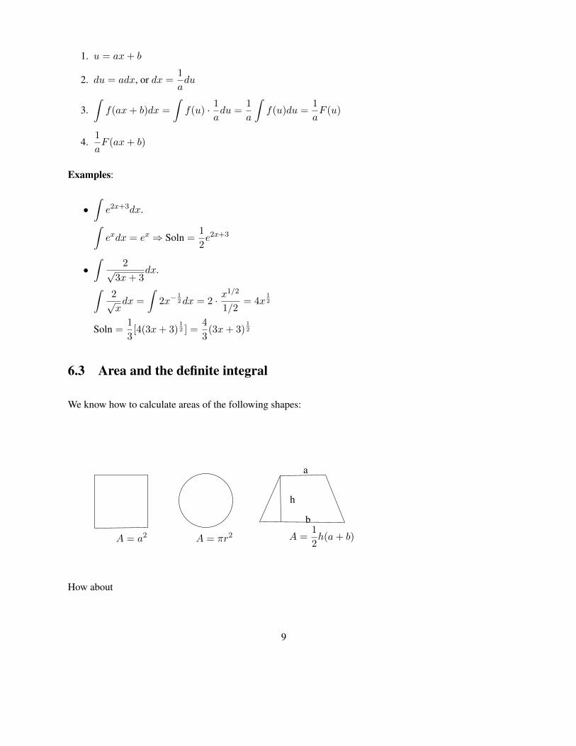
6.3 Area and the definite integral

We know how to calculate areas of the following shapes:

a

b

h

A =1

2h(a+ b)A = πr2A = a2

How about

9

1 2

1

2

0

f

Example 1 Compute the area of the region bounded by y = 0.5x2, x = 1, x = 2 and x-axis.

Method:Approximation.

Procedure:

1. divide [1, 2] into n = 1 subinterval.Let x1 = 1, x2 = 2,

∆x =2− 1

n= 1 (length of subintervals)

A ' ∆xf(x1) = ∆x · 0.5x21 = 0.5.

1 2

1

2

0

f(x1)

f(x2)

x1 x2

f

10

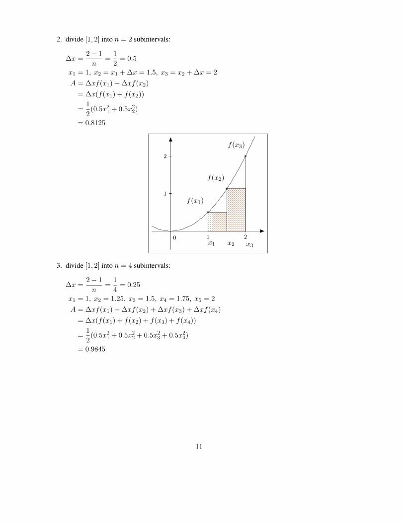
2. divide [1, 2] into n = 2 subintervals:

∆x =2− 1

n=

1

2= 0.5

x1 = 1, x2 = x1 + ∆x = 1.5, x3 = x2 + ∆x = 2

A = ∆xf(x1) + ∆xf(x2)

= ∆x(f(x1) + f(x2))

=1

2(0.5x2

1 + 0.5x22)

= 0.8125

1 2

1

2

0

f(x1)

f(x2)

x1 x2 x3

f(x3)

f

3. divide [1, 2] into n = 4 subintervals:

∆x =2− 1

n=

1

4= 0.25

x1 = 1, x2 = 1.25, x3 = 1.5, x4 = 1.75, x5 = 2

A = ∆xf(x1) + ∆xf(x2) + ∆xf(x3) + ∆xf(x4)

= ∆x(f(x1) + f(x2) + f(x3) + f(x4))

=1

2(0.5x2

1 + 0.5x22 + 0.5x2

3 + 0.5x24)

= 0.9845

11

1 2

1

2

0

f

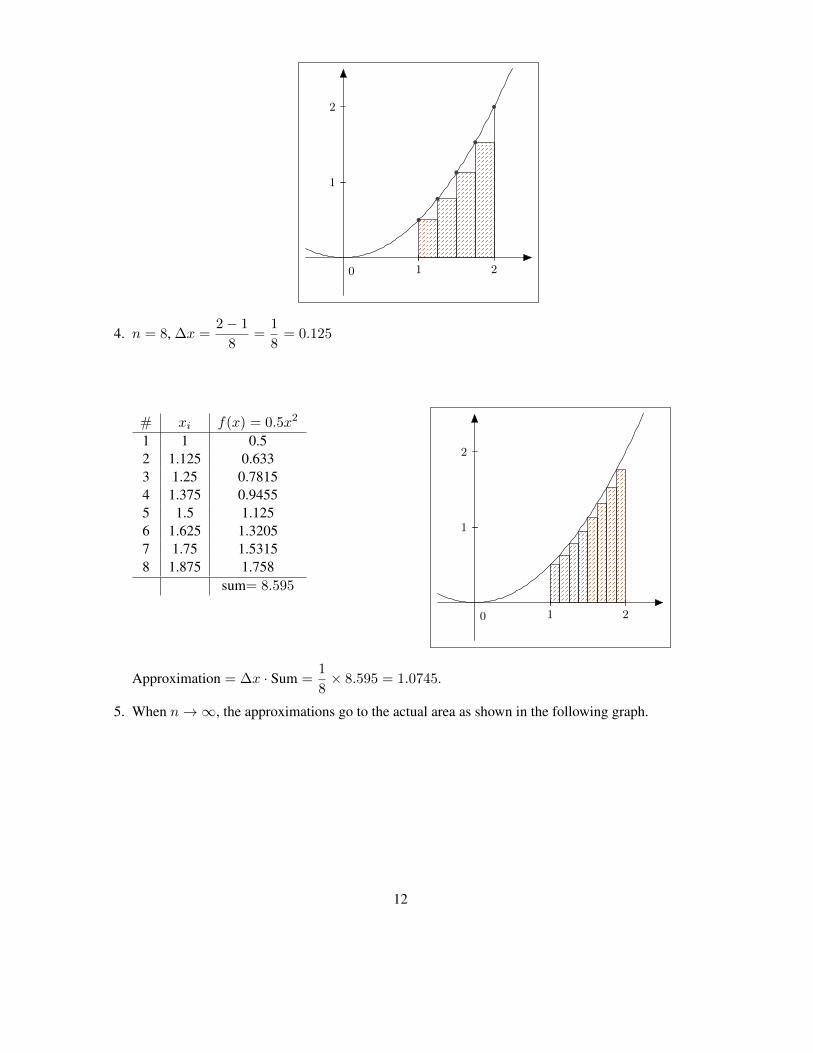
4. n = 8, ∆x =2− 1

8=

1

8= 0.125

# xi f(x) = 0.5x2

1 1 0.52 1.125 0.6333 1.25 0.78154 1.375 0.94555 1.5 1.1256 1.625 1.32057 1.75 1.53158 1.875 1.758

sum= 8.595

1 2

1

2

0

f

Approximation = ∆x · Sum =1

8× 8.595 = 1.0745.

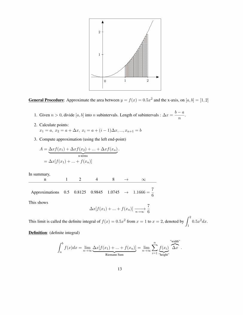
5. When n→∞, the approximations go to the actual area as shown in the following graph.

12

1 2

1

2

0

General Procedure: Approximate the area between y = f(x) = 0.5x2 and the x-axis, on [a, b] = [1, 2]

1. Given n > 0, divide [a, b] into n subintervals. Length of subintervals : ∆x =b− an

.

2. Calculate points:x1 = a, x2 = a+ ∆x, xi = a+ (i− 1)∆x, ..., xn+1 = b

3. Compute approximation (using the left end-point)

A = ∆xf(x1) + ∆xf(x2) + ...+ ∆xf(xn)︸ ︷︷ ︸n terms

.

= ∆x[f(x1) + ...+ f(xn)]

In summary,n 1 2 4 8 → ∞

Approximations 0.5 0.8125 0.9845 1.0745 → 1.1666 =7

6

This shows∆x[f(x1) + ...+ f(xn)] −−−→

n→∞

7

6

This limit is called the definite integral of f(x) = 0.5x2 from x = 1 to x = 2, denoted by∫ 2

10.5x2dx.

Definition: (definite integral)

∫ b

af(x)dx = lim

n→∞∆x[f(x1) + ...+ f(xn)]︸ ︷︷ ︸

Riemann Sum

= limn→∞

n∑i=1

f(xi)︸ ︷︷ ︸”height”

”width”︷︸︸︷∆x .

13

Heren∑

i=1

∆x = b− a, or ∆x =b− an

Existence Theorem: If f is continuous on [a, b], then the definite integral∫ b

af(x)dx exists, or f is

integrable on [a, b].

Geometric interpretation:

Generally speaking:∫ b

af(x)dx is not the area of the region bounded by y = f(x), x = a, x = b and

x-axis. It is the area above the x-axis minus the area below the x-axis.

Example The area of the region below = 1. However∫ 1

0(−x+ 1)dx = 0

1 2

−1

1

0

y = f(x) = −x+ 1

Actually, if f(x) ≥ 0 on [a, b], then∫ b

af(x)dx is the area of the region bounded by y = f(x), x = a,x =

b and the x-axis. if f(x) ≤ 0 on [a, b], then∫ b

af(x)dx is negative of the area of the region bounded by

y = f(x), x = a,x = b and the x-axis.∫ 1

0(−x+ 1)dx =

1

2b · h =

1

2· 1 · 1 =

1

2∫ 2

1(−x+ 1)dx = −1

2b · h = −1

2· 1 · 1 = −1

2∫ 2

0(−x+ 1)dx =

∫ 1

0(−x+ 1)dx+

∫ 2

1(−x+ 1)dx = 0

14

6.4 The fundamental theorem of Calculus

Theorem Let F (x) be any antiderivative of f(x): F ′(x) = f(x). Then∫ b

af(x)dx = F (x)|ba ≡ F (b)− F (a). (definite integral, which has unique value)

Example 1 : Find the area of the region bounded by y = x2, x = 1, x = 2 and the x-axis.

A =

∫ 2

1x2dx =

x3

3

∣∣∣∣21

=23

3− 13

3=

7

3

Example 2 Find the area of the region bounded by y = −x2 + 4, x = 1, x = 3 and the x-axis.

−x2 + 4 = 0, x2 = 4, x = ±2

Area 6=∫ 3

1(−x2 + 4)dx

Area =

∫ 2

1(−x2 + 4)dx−

∫ 3

2(−x2 + 4)dx

Example 3 : Find the area of the region bounded by y = x2 + 1 from x = −1 to x = 2.

A =

∫ 2

−1(x2 + 1)dx =

x3

3

∣∣∣∣2−1

+ x|2−1 =23

3− (−1)3

3+ (2− (−1)).

Example 4 Calculate∫ 3

1(3x2 + ex)dx.

∫ 3

1(3x2 + ex)dx =

3x3

3

∣∣∣∣31

+ ex|31 = 33 − 13 + e3 − e1 = 26 + e3 − e.

Example 5: Find the area of region bounded by the graph of y = −x2, x = −1, x = 2 and the x-axis.

−2 −1 1 2 3

−4

−2

0

y = 0

y = −x2

15

Soln:

A =

∫ 2

−1[0− (−x2)]dx =

x3

3

∣∣∣∣2−1

=23

3− (−1)3

3= 3.

Note that area is always a positive number. But the integral of −x2 over [−1, 2] is negative.∫ 2

−1−x2dx = −3.

Ex 3: Find the area of the region bounded by y = −x+ 1, x = 0, x = 2 and x-axis.

1 2

−1

1

0

Note that the integral∫ 2

0(−x+ 1)dx is positive in the black region and negative in the red region. So the

area is the sum absolute value of these two parts, which leads to

A =

∫ 1

0(−x+ 1)dx+

[−∫ 2

1(−x+ 1)dx

]= 2

or

A =

∣∣∣∣∫ 1

0(−x+ 1)dx

∣∣∣∣+

∣∣∣∣∫ 2

1(−x+ 1)dx

∣∣∣∣ = 2

Ex 4: Find the area enclosed by the graph of f(x) and x-axis on the interval [a, b].

(a) f(x) = (x− 1)(x− 3), [0, 4]

• Find the roots of f(x) = 0: (x− 1)(x− 3) = 0, x = 1, 3

• x = 1, 3 divides [0, 4] into [0, 1], [1, 3] and [3, 4].

• Find the area of each interval and add them up:

Area=∣∣∣∣∫ 1

0f(x)dx

∣∣∣∣+

∣∣∣∣∫ 3

1f(x)dx

∣∣∣∣+

∣∣∣∣∫ 4

3f(x)dx

∣∣∣∣(b) f(x) = (x− 1)(x− 3), [2, 4]

• Find the roots of f(x) = 0: x = 1, 3.

• x = 1, 3 divides [2, 4] into [2, 3] and [3, 4].

16

• Area=

∣∣∣∣∫ 3

2f(x)dx

∣∣∣∣+∣∣43f(x)dx

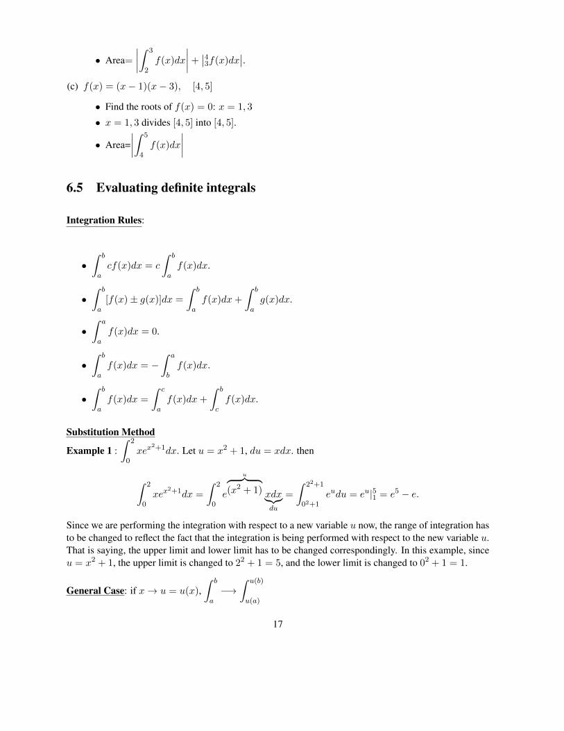
∣∣.(c) f(x) = (x− 1)(x− 3), [4, 5]

• Find the roots of f(x) = 0: x = 1, 3

• x = 1, 3 divides [4, 5] into [4, 5].

• Area=∣∣∣∣∫ 5

4f(x)dx

∣∣∣∣6.5 Evaluating definite integrals

Integration Rules:

•∫ b

acf(x)dx = c

∫ b

af(x)dx.

•∫ b

a[f(x)± g(x)]dx =

∫ b

af(x)dx+

∫ b

ag(x)dx.

•∫ a

af(x)dx = 0.

•∫ b

af(x)dx = −

∫ a

bf(x)dx.

•∫ b

af(x)dx =

∫ c

af(x)dx+

∫ b

cf(x)dx.

Substitution Method

Example 1 :∫ 2

0xex

2+1dx. Let u = x2 + 1, du = xdx. then

∫ 2

0xex

2+1dx =

∫ 2

0e

u︷ ︸︸ ︷(x2 + 1) xdx︸︷︷︸

du

=

∫ 22+1

02+1eudu = eu|51 = e5 − e.

Since we are performing the integration with respect to a new variable u now, the range of integration hasto be changed to reflect the fact that the integration is being performed with respect to the new variable u.That is saying, the upper limit and lower limit has to be changed correspondingly. In this example, sinceu = x2 + 1, the upper limit is changed to 22 + 1 = 5, and the lower limit is changed to 02 + 1 = 1.

General Case: if x→ u = u(x),∫ b

a−→

∫ u(b)

u(a)

17

Example 2:∫ 1

−1x2(x3 + 1)4dx.

Let u = x3 + 1, du = 3x2dx.∫ 1

−1x2(x3 + 1)4dx =

∫ 1

−1(x3 + 1︸ ︷︷ ︸

u

)4 x2dx︸ ︷︷ ︸13du

=

∫ 2

0

1

3u4du

=1

3

u5

5

∣∣∣∣20

=1

3

(25

5− 05

5

)=

32

15.

Average of a function:

average of f(x) on [a, b] ' f(x1) + f(x2) + ...+ f(xn)

n

=1

b− a∆x[f(x1) + ...+ f(xn)]︸ ︷︷ ︸

Riemann Sum

, ∆x =b− an

⇒ 1

b− a

∫ b

af(x)dx.

average of f(x) on [a, b] =1

b− a

∫ b

af(x)dx.

Example 1: A car is traveling at a velocity v(t) from time a to b. Find the average velocity of this carduring this time period.

Soln:

• Total Distance=

∫ b

av(t)dt

• average velocity =Total Distance

Total time=

∫ ba v(t)dt

b− a

Examples

•∫ 2

0xe2x2

dx

•∫ 1

0

x2

x3 + 1dx

•∫ 4

0x√

9 + x2dx

18

6.6 Area between two curves

∫ b

af(x)dx is the area of the region bounded by y = f(x), x = a, x = b and x-axis. If f(x) ≥ 0, for all

x ∈ [a, b].

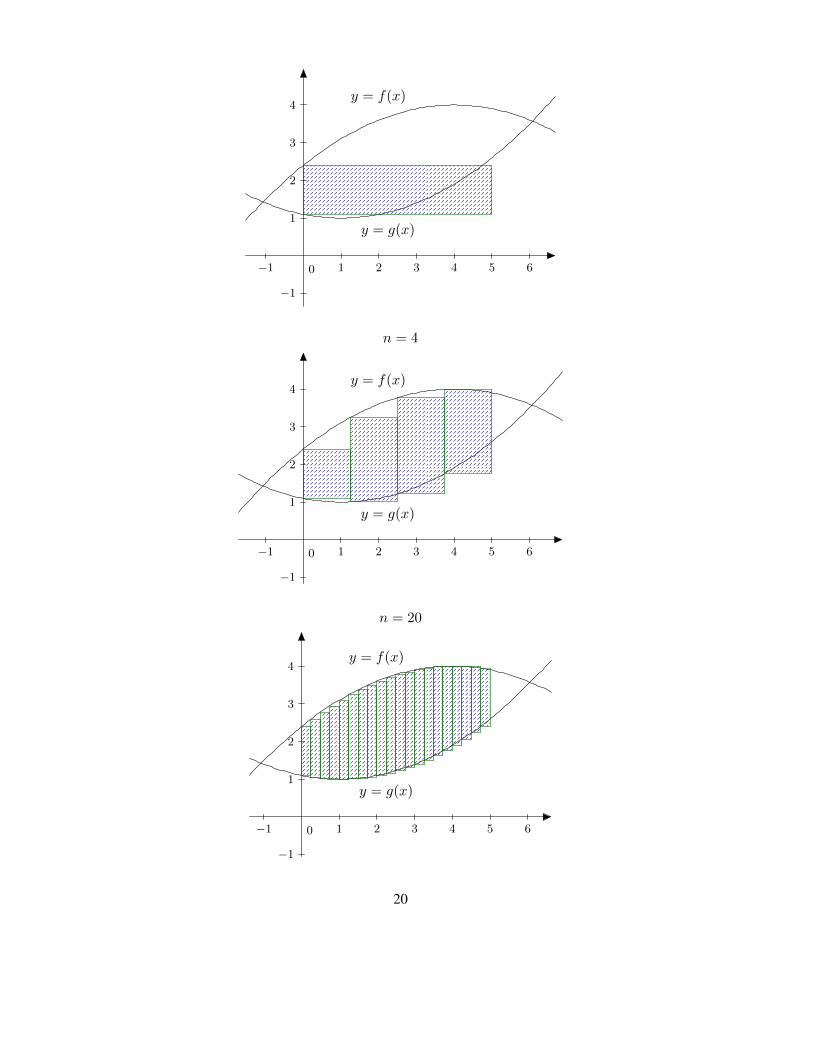
Finding the area between two curves: If f(x) ≥ g(x) on [a, b], then the area of the region boundedabove by y = f(x) and below by y = g(x) on [a, b] is given by∫ b

a[f(x)− g(x)]dx

−1 1 2 3 4 5 6

−1

1

2

3

4

5

0

y = f(x)

y = g(x)

Approximation: Height=f(x)− g(x), width=∆x =b− an

.

Area 'n∑

i=1

[f(xi)− g(xi)] ∗b− an

∫ b

af(x)− g(x)︸ ︷︷ ︸

”Height”

”width”︷︸︸︷dx = lim

n→∞

n∑i=1

f(xi)− g(xi)∆x

n = 1

19

−1 1 2 3 4 5 6

−1

1

2

3

4

0

y = f(x)

y = g(x)

n = 4

−1 1 2 3 4 5 6

−1

1

2

3

4

0

y = f(x)

y = g(x)

n = 20

−1 1 2 3 4 5 6

−1

1

2

3

4

0

y = f(x)

y = g(x)

20

Example 1: Find the area of the region that is completely enclosed by the graphs of y = 2x − 1 andg(x) = x2 − 4.

−4 −3 −2 −1 1 2 3 4 5

−4

−2

2

4

6

0

y = 2x− 1

y = x2 − 4A1

A2

Soln: We first find out the intersection point of these two curves by solving

2x− 1 = x2 − 4,

x2 − 2x− 3 = 0,

(x− 3)(x+ 1) = 0,

x = −1, 3.

Then A =

∫ 3

−1[(2x− 1)− (x2 − 4)]dx.

Example 2: Find the area of the region completely enclosed by the graphs of the functions f(x) =x3 − 3x+ 3, and g(x) = x+ 3

21

−3 −2 −1 1 2 3 4 5

2

4

6

0

f(x) = x3 − 3x+ 3 g(x) = x+ 3

A1

A2

A3

We get the x-values of the points of intersection of f(x) and g(x) by solving

x3 − 3x+ 3 = x+ 3

x3 − 4x = 0⇒ (x2 − 4)x = 0⇒ (x− 2)(x+ 2)x = 0

x = −2, 0, 2.

In the red region, since f(x) ≥ g(x), its area is∫ 0

−2f(x)−g(x)dx. In the black region, since g(x) ≥ f(x),

its area is∫ 2

0g(x)− f(x)dx. So

A =

∫ 0

−2f(x)− g(x)dx+

∫ 2

0g(x)− f(x)dx = 8

Examples

(a) f(x) = x√x+ 2, g(x) = x2

• f(x) = g(x), x√x+ 2 = x2, x(

√x+ 2− x) = 0

⇒ x = 0, or√x+ 2− x = 0√

x+ 2 = x, x+ 2 = x2, x2 − x− 2 = 0, (x− 2)(x+ 1) = 0, x = −1, 2

However, x = −1 is not a solution because√−1 + 2 6= −1.

x = 0, 2

22

• A =

∣∣∣∣∫ 2

0x√x+ 2− x2dx

∣∣∣∣(b) f(x) = x3 − 3x, g(x) = 2x2

• f(x) = g(x), x3 − 2x2 − 3x = 0, x(x− 3)(x+ 1) = 0, x = −1, 0, 3

• Area=

∣∣∣∣∫ 0

−1f(x)− g(x)dx

∣∣∣∣+

∣∣∣∣∫ 3

0f(x)− g(x)dx

∣∣∣∣6.7 Applications of the Definite integral to Business and Economics

Consumers’ and Producers’ Surplus:

Consumers’ Surplus:

Demand function — relates unit price p of a commodity to the quantity x demanded of it.{if p is high, x is smallif p is low, x is large

p = D(x) indicates how much people is willing to pay for the unit price at a level quantity x. Supposethat a fixed unit market price p̄ has been established for the commodity and the corresponding quantitydemanded is x̄. Thus

the actual payment by consumers = p̄x̄

the amount consumers are willing to pay =

∫ x̄

0D(x)dx.

consumers’ Surplus = amount consumers are willing to pay

− amount consumers actually pay

=

∫ x̄

0D(x)dx− p̄x̄.

10 20 30

10

20

30

0

x̄

p̄

Demand function p = D(x)(willing to pay)

23

10 20 30

10

20

0x̄

p̄

consumerssurplus

10 20 30

10

20

0x̄

p̄

consumersactually pay

10 20 30

10

20

0x̄

p̄

consumerswilling to pay

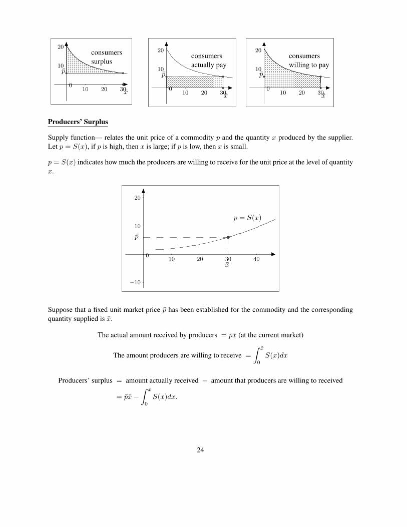
Producers’ Surplus

Supply function— relates the unit price of a commodity p and the quantity x produced by the supplier.Let p = S(x), if p is high, then x is large; if p is low, then x is small.

p = S(x) indicates how much the producers are willing to receive for the unit price at the level of quantityx.

10 20 30 40

−10

10

20

0

x̄

p̄

p = S(x)

Suppose that a fixed unit market price p̄ has been established for the commodity and the correspondingquantity supplied is x̄.

The actual amount received by producers = p̄x̄ (at the current market)

The amount producers are willing to receive =

∫ x̄

0S(x)dx

Producers’ surplus = amount actually received − amount that producers are willing to received

= p̄x̄−∫ x̄

0S(x)dx.

24

10 20 30

10

0x̄

p̄

Actual received

10 20 30

10

0x̄

p̄

Willing to receive

10 20 30

10

0x̄

p̄

Producers’ surplus

Example 1 The demand function for a commodity is

p = D(x) = −0.001x2 + 250

where p is the unit price in dollars and x is the quantity demanded in units of a thousand. The supplyfunction for the commodity is

p = S(x) = 0.0006x2 + 0.02 + 100

Determine the consumers’ and producers’ surplus if the market price of the commodity is set at the equi-librium price.

25

p̄

x̄x1 x2

D(x)

S(x)

• x1: supply < demand, x ↑

• x2: supply > demand, x ↓

• x̄: supply = demand, market price, stable.

Soln: x̄ is the solution of S(x) = D(x). Solve the equation, we get x =−625

2, 300. Since x̄ can’t be

negative, x̄ = 300. And p̄ = D(x̄) = 160.

Consumers’ surplus =

∫ 300

0D(x)dx− p̄x̄ = 18, 000.

Producers’ surplus = p̄x̄−∫ 300

0S(x)dx = 11, 700.

The future and present value of an income stream

• a firm generates a stream of income over a period of time.

R(t) — rate of income generation at time t. E.g., R(t) = 3000 dollar/hour.

• The realized income is reinvested (in the bank) and earns interest at a fixed rate:

r — interest rate compounded continuously

• The period of time = T

26

• If put in the bank, and interest is compounded continuously,

Total interest + Principle = Principal · ert

Principal: the initial money you borrowed from or deposited to the bank.

t is the total amount of time.

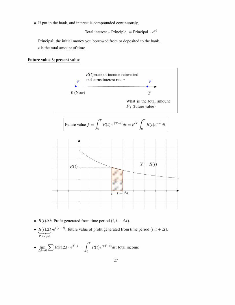
Future value & present value

0 (Now) T

What is the total amountF ? (future value)

R(t)=rate of income reinvestedand earns interest rate rP F

Future value f =

∫ T

0R(t)er(T−t)dt = erT

∫ T

0R(t)e−rtdt.

t t+ ∆t

R(t)Y = R(t)

• R(t)∆t: Profit generated from time period (t, t+ ∆t).

• R(t)∆t︸ ︷︷ ︸Principal

·er(T−t): future value of profit generated from time period (t, t+ ∆).

• lim∆t→0

∑R(t)∆t · eT−t =

∫ T

0R(t)er(T−t)dt: total income

27

Present Value

0 (Now)Present value P = ?

T

future value F

R(t)=rate of income reinvestedand earns interest rate rP F

The present value P that will yield the same accumulated value as the income stream itself when P isinvested for the same period of time at the same rate of interest.

PerT = F = erT∫ T

0R(t)e−rtdt

⇒ P =

∫ T

0R(t)e−rtdt .

Example 2: The owner of a local cinema is studying a plan for renovating and improving the theater. theplan calls for an immediate outlay of $ 250,000. It has been estimated that the plan would result in a netincome stream generated at the rate of

R(t) = $630, 000 per year

If the prevailing interest rate for the next 5 years is 10% annually, determine the net income in the presentvalue and the futher value at the end of 5 years.Soln:

R(t) = $630, 000, r = 0.1, T = 5

Future value of the plan F = e0.1×5

∫ 5

0630, 000e−0.1tdt

= 1, 632, 845× e0.1×5

= 2, 692, 106

future value of the cost 250, 000 if put in the bank B = 250000e0.1∗5 = 412, 180.

A−B = 2, 279, 926 (future value of profit)

present value P =

∫ 5

0630, 000e−0.1tdt = 1, 632, 845

P − cost = 1, 632, 845− 250, 000 = 1, 382, 845

28

Review: Chapter 5 & 6

• e ' 2.7182818

• ex

ex+y = exey

ex−y =ex

ey(ex)y = exy

d

dx= ex,

d

dxef(x) = ef(x)f ′(x)

• lnx

ln(xy) = lnx+ ln y

ln

(x

y

)= lnx− ln y

lnxy = y lnxd

dxlnx =

1

xd

dxln f(x) =

1

f(x)f ′(x)

• Relation:ln ex = x, elnx = x.

• Chapter 6 Integration: see page 543–544

• Problems: (Review of chapter 6, Page 544–547) 14, 32, 34, 38, 50.

Review: Integration

Concepts:

• differentiation↔ integration.

• antiderivatives F ′(x) = f(x).

• indefinite integral∫f(x)dx = F (x) + C.

• definite integral∫ b

af(x)dx = F (b)− F (a).

• Riemann Sum

• relation between area and definite integral.

• Consumers’ surplus: CS =

∫ x̄

0D(x)dx− p̄x̄.

29

• Producers’ surplus: PS = p̄x̄−∫ x̄

0S(x)dx.

• Present Value: P =

∫ T

0R(t)e−rtdt.

• Future Value: F = erT∫ T

0R(t)e−rtdt.

Integration Techniques:

•∫f(x)± g(x)dx =

∫f(x)dx+

∫g(x)dx.

•∫cf(x)dx = c

∫f(x)dx.

•∫

1dx = x+ C.

•∫xndx =

xn+1

n+ 1+ C, n 6= −1.

•∫

1

xdx = ln(x) + C.

•∫exdx = ex + C.

•∫eaxdx =

1

aeax + C, a 6= 0.

•∫ a

af(x)dx = 0.

•∫ b

af(x)dx = −

∫ a

bf(x)dx.

•∫ b

af(x)dx =

∫ c

af(x)dx+

∫ b

cf(x)dx.

• Method of substitution.

• fundamental theorem of calculus:∫ b

af(x)dx = F (x)|ba = F (b)− F (a).

Applications:

• Compute areas between curves.

30

• compute CS, PS, FV,PV

• average=1

b− a

∫ b

af(x)dx.

31