1

Math 216 - Assignment 1 - Introduction to MATLAB

Due: Monday, January 29. Nothing accepted after Tuesday, January 30. This is worth 15

points. 10% points off for being late. You may work by yourself or in pairs. If you

work in pairs it is only necessary to turn in one set of answers for each pair. Put both

your names on it.

Do Problems 1 - 22 in the discussion below. Copy and paste the input and output for each

problem from the Command Window (or plot window) to a Microsoft Word file. Do this

after you are satisfied with your input and output. Label the work for each problem in the

Word file: Problem 1, Problem 2, etc. Print a copy of this file to hand in. An alternative

to copying and pasting into a Word file is to use the MATLAB Live Script feature

discussed at the end.

MATLAB is a program for doing mathematical computations.

To start:

1. On a Mac: Bring up Spotlight Search by entering Command-Space. Enter "MATLAB".

The version of MATLAB on your computer should fill in at the top. Press Return to start

MATLAB. Another possibility is to use the Finder to open the Applications folder.

Double-click on the MATLAB version in that folder.

2. On a PC: Click the Start button in the lower left. Depending on the version of Windows

either a list of programs should appear or you may have to look around (e.g click a down

arrow or select All Programs) to bring up that list. On the program list select the version

of MATLAB available.

To exit: Save any work you might want to use later and select Exit in the File menu.

When you start, the MATLAB window is divided into several sub-windows. The most

important one is the Command Window where you enter expressions (often referred to as

commands, statements or lines). The expressions are evaluated and the results are displayed.

The Command Window is usually in the middle of the MATLAB window. Another window is

the Workspace Window where variables are displayed with their values. There is also the

Current Folder Window where files will be saved if you don't specify otherwise. Also present

may be the Command History Window where previously entered commands are displayed

although this may be a pop-up window which appears when you use the up arrow key. If you are

working with a script or Live Script, it will be in the Editor Window above the Command

Window

Computations

In the Command Window, you will see a prompt followed by a blinking cursor:

>> |

2

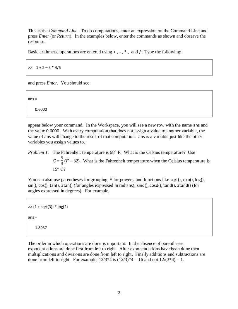
This is the Command Line. To do computations, enter an expression on the Command Line and

press Enter (or Return). In the examples below, enter the commands as shown and observe the

response.

Basic arithmetic operations are entered using + , - , * , and / . Type the following:

>> 1 + 2 – 3 * 4/5

and press Enter. You should see

ans =

0.6000

appear below your command. In the Workspace, you will see a new row with the name ans and

the value 0.6000. With every computation that does not assign a value to another variable, the

value of ans will change to the result of that computation. ans is a variable just like the other

variables you assign values to.

Problem 1: The Fahrenheit temperature is 68 F. What is the Celsius temperature? Use

C = 5

9 (F – 32). What is the Fahrenheit temperature when the Celsius temperature is

15 C?

You can also use parentheses for grouping, ^ for powers, and functions like sqrt(), exp(), log(), sin(), cos(), tan(), atan() (for angles expressed in radians), sind(), cosd(), tand(), atand() (for

angles expressed in degrees). For example,

>> (1 + sqrt(3)) * log(2) ans = 1.8937

The order in which operations are done is important. In the absence of parentheses

exponentiations are done first from left to right. After exponentiations have been done then

multiplications and divisions are done from left to right. Finally additions and subtractions are

done from left to right. For example, 12/3*4 is (12/3)*4 = 16 and not 12/(3*4) = 1.

3

>> 12/3*4 ans = 16

Problem 2: An equilateral triangle has area 6 m2. What is the length of the side?

Problem 3: A tree 20 feet tall casts an 8 foot shadow. What is the angle of elevation of the sun?

Express the answer both in radians and degrees.

Problem 4: A certain amount is invested in a savings account with an annual interest rate of

1%. It is compounded quarterly. After 10 years it has grown to $2,000. What is

the original amount? Use the formula An = A0 (1 + i

c)nc, where A0 is the original

amount, An is the amount after n years, i is the annual interest rate and c is the

number of times a year it is compounded.

You may use the word pi for the special number 3.14159…. If you are familiar with

Mathematica, you may notice that the syntax in MATLAB is frequently different. You should

not capitalize functions or predefined constants like pi, nor use square brackets for the inputs to

functions. For example, in MATLAB one would enter sin(pi/8) while in Mathematica one

would enter Sin[Pi/8] for the same thing.

What happens when you enter the following command?

>> sin(2pi)

The problem here is that multiplication always needs to be explicitly entered using a *. Note that

MATLAB suggests a correction for you. In this case it was the right one. Let's try the suggested

correction:

>> sin(2*pi)

Is the answer what you expected?

There is a new problem, i.e. the answer is not zero. Most real numbers that are not integers are

not represented exactly in most programming languages including MATLAB. Rather they are

represented in floating point form with only a fixed number of digits. 16 digits is common in

many programming languages including MATLAB. These are called double precision floating

point numbers. So, numerical computations with real numbers in MATLAB are limited to 16

4

digits of precision. In particular, 2*pi does not represent 2 exactly. Rather it represents a

number that agrees with 2 to 16 digits. The error is on the order of 10-16 and is called round-off

error. So when sin(2*pi) is evaluated the result again differs from 0 by an amount on the order of

10-16, again a round-off error.

This effect is magnified with larger multiples of π: Try the following.

>> sin(8*10^15*pi)

As you can see, with very large multiples of , the round-off error is so large that the result is

unusable.

Problem 5: Find the radius of a sphere whose volume is 8 m3. Recall V = 4

3 r3.

i and j both can be used for - 1. However, for e = 2.71828… you need to use exp(1).

Even though MATLAB represents numbers with 16 digits of precision, it normally only prints

out four digits to the right of the decimal point or the four most significant digits. This can be

changed. For example, if you enter the command "format long" then future output will have 16

digits of precision. Later, if you enter the command "format short" it reverts to four digits.

Another option is to enter "format rat" in which case future output is printed out to a rational

number very close to the actual floating point value. For example,

>> 1 + 2 – 3 * 4/7 ans =

1.2857 format long >> 1 + 2 – 3 * 4/7 ans =

1.285714285714286 >> format rat >> 1 + 2 - 3*4/7 ans = 9/7

5

Often one wants to repeat a previously entered expression or command, perhaps with

modifications. This can be done as follows. When one has the prompt on the Command Line,

press the up arrow. The previously entered command appears on the command line. By

repeated presses of the up and down arrows one can scroll through the command history until the

desired expression appears to the right of the prompt. Make any modifications using the right

and left arrows and backspace keys and press enter.

What do you expect from the following computation?

>> (-8)^(1/3)

Based on previous mathematics courses, you would probably simplify this to −2. If we consider

complex numbers, however, there are three cube roots of -8. These are −2 and 1 + 3 i and

1 - 3 i. In situations like this MATLAB gives the value with the largest positive real part and

positive imaginary part.

If you want the real cube root of a negative number, like -8, you can enter – 8^(1/3) in which

case it finds the positive cube root of 8 and negates it. If the number is the value of some

variable, say x and you don't know if it is positive or negative you can enter sign(x)*abs(x)^(1/3). Here sign(x) is 1 if x is positive, 0 if x is zero and -1 if x is negative.

Problem 6: Compute 2 + 3i

3 - 4i in standard complex form.

Variables

Like all programming languages, MATLAB allows one to use variables to hold values to be used

in later computations. For example, entering the following

>> a = sqrt(3)

assigns the value 1.732.. to the variable a. Note that this is reflected by a new entry in the

Workspace. Once the variable a has been assigned this value we can use it in computations that

follow. For example, what do you get when you enter the following.

>> (a^3-2*a)^(-2)

Can you verify the answer by a hand computation?

6

Problem 7: Use one or more variables to compute the surface area of a sphere whose volume is

8 m3. Recall A = 4r2.

When we don't need to repeat the value we assign to a variable, we can suppress the output using

a semicolon:

>> temperature = 72;

Variable names can be any string of letters and numbers beginning with a letter. For example,

>> r2d2 = 1001

This can cause problems if you are not careful. For example, if you assign a value to a variable

whose name is the name of one of a function, then that name becomes unusable for that function.

Try the following.

>> cos = 14 >> cos(pi) Subscript indices must either be real positive integers or logicals.

The error message that is mysterious at first, but it becomes understandable as we get to know

more about MATLAB. MATLAB, which was first developed to work with vectors and

matrices, interprets cos(pi) as a reference to the πth entry in the vector assigned to the variable

cos. Even though 14 is a number, MATLAB interprets it a vector with only one component.

Subscripts for a vector can only be positive integers, so MATLAB is complaining that the th

entry of a vector doesn't make sense.

Note that when we assigned 14 to the variable cos, this was reflected in the Workspace window.

As we mentioned, assigning 14 to the variable cos, makes the cosine function unusable. We can

undo this definition in two ways. From the Workspace, you can click on cos and enter Delete, or

right-click (control-click on a Mac) on cos and select Delete from the pop-up menu.

Alternatively, from the Command Window, you can enter

>> clear cos

and it will disappear from the Workspace.

7

The variables and their values in the Workspace can be saved for later use by a command of the

form save(filename) where filename is the name of the file where the variables will be stored.

When you enter this command a file with the name filename.mat will appear in the Current

Folder. At a future MATLAB session you can load these variables back into the Workspace

with the command load(filename). (This didn't seem to work in 2048 CB.)

Vectors

Recall that a vector is (or can be represented by) a list of numbers. The individual numbers are

called the components of the vector. For example, (3, 1, 4, 1, 5, 9) is a row vector with six

components and

2

7

1

8

2

8

is a column vector also with six components. To represent a row vector in

MATLAB, we enter the components enclosed in square brackets. The components may be

separated by spaces or commas. For example, the following assigns the row vector

(3, 1, 4, 1, 5, 9) to the variable v. Notice how MATLAB echoes the values assigned to v.

>> v = [3, 1, 4, 1, 5, 9];

v = 2 7 1 8 2 8

The variable v has also been added to the Workspace with its value.

Often we can get along with just row vectors. However, when we start doing matrix

computations, then it is handy to be able to distinguish between row and column vectors. To

define a column vector we use semicolons instead of commas to separate the components. This

assigns the column vector

2

7

1

8

2

8

to u.

>> u = [2; 7; 1; 8; 2; 8]; u = 2 7 1 8 2 8

8

If the value of a variable u is a vector and i is a positive integer, then u(i) refers to the ith

component of u. For example, the following command adds the 2nd component of u and the 3rd

component of v.

>> u(2) + v(3)

Problem 8: A vector p = [p1, p2] has magnitude 3 and makes an angle of 40 with the positive x

axis. Enter p into the Command Line as p = [p1, p2] where p1 and p2 are numbers

you need to compute.

When the components of a vector are evenly spaced, there is a way to avoid writing them all out.

For example, 3:2:15 is short for the vector [3, 5, 7, 9, 11, 13, 15].

>> a = 3:2:15

Problem 9: Create a vector whose components are the multiples of 7 from 21 to 105.

If the components are consecutive integers, one can omit the increment in the middle. For

example 0:10 stands for the vector [0, 1, 2, 3, 4, 5, 6, 7, 8, 9, 10].

>> c = 0:10

Problem 10: Create a vector whose components are the consecutive integers from 21 to 35.

What happens if the last component cannot be obtained by adding a multiple of the increment to

the first component. Try the following.

>> w = 5:2:10

Another way to define vectors whose components are equally spaced is to use the linspace

function. With linspace one specifies the first and last component of the vector along with the

total number of components in the vector. For example,

>> z = linspace(2,4,6)

z = 2.0000 2.4000 2.8000 3.2000 3.6000 4.0000

9

Problem 11: Create a vector with 8 equally spaced components beginning with 6 and ending

with 9.

There are many vector operations. For example, if v and z are vectors with the same number of

components, then v + z is the usual vector sum of v and z, i.e. the vector whose components are

the sums of the corresponding components of v and z. Similarly, v - z is the usual vector

difference of v minus z. If t is a number then t*v is the usual product of the number t times the

vector v. For example, here is the sum of the vectors v and z above.

>> v + z ans =

5.0000 3.4000 6.8000 4.2000 8.6000 13.0000

Problem 12: An object is acted upon by a force F1 of magnitude 3 making an angle of 40 with

the positive x axis. At the same time it is also acted upon by a force F2 of

magnitude 4 making an angle of 111 with the positive x axis. Find a single force

F which when acting on the object has the same effect on the object as the forces

F1 and F2 combined. Specify F by giving its components in the x and y directions

and also its magnitude and direction.

When we get to multiplication, division and exponentiation, things are a little different. For

example, v * z is not the usual scalar product of v and z. In fact it is undefined in MATLAB if v

and z are vectors of the same type. If v is a row vector and z is a column vector than v * z is the

usual product of a row and column vector, i.e. the sum of the products of the corresponding

components which is the same as the scalar product of the v and the transpose of z.

However, if we put a period in front of the * so it is v .* z, then this is the vector obtained by

multiplying the corresponding components of v and z, i.e. (v .* z)(i) equals v(i) * z(i). The

products are not summed like in the scalar product. For example

[2, 3, 4] .* [5, 6, 7] = [10, 18, 28]. This operation is not as common in linear algebra books, but

has many uses. A similar thing happens with division, v ./ z, is the vector obtained by dividing

the corresponding components of v and z, i.e. (v ./ z)(i) equals v(i) / z(i). These are examples of

component-wise operation.

If t is a number and v is a vector, then v + t, v - t, t - v, t*v and v/t are the vectors obtained by

adding t to each of the components of v, subtracting t from each of the components of v,

subtracting each of the components of v from t, multiplying each of the components of v by t and

dividing each of components of v by t. However one needs the period as in t ./ v and v .^ t to

create the vectors whose components are t divided by each of the components of v and each of

the components of v raised to the power t. For example,

10

>> [1, 2, 3] .^ 2 ans =

1 4 9

Having to use a period before the *, / and ^ is a bit of a nuisance when translating formulas from

mathematical notation to MATLAB when plotting and doing other vector computations. We

shall see more examples of this in the next section on plotting.

Another example of a component-wise operation on vectors is to apply a function to a vector.

This gives the vector obtained by applying the function to each of the components separately.

For example,

>> y = [1, 2, 3]; >> sin(y) ans =

0.8414 0.9093 0.1411

Problem 13: Create a vector whose components are the square roots of the integers from 1 to 10.

We look more at vector operations in Lab 3.

Plotting

Making graphs is done with the plot function. To make the graph of a function y = f(x) over an

interval a x b, first divide up the interval into a number of equally spaced points

x1 < x2 < … < xn where x1 = a and xn = b. These points are stored in a vector x. The number n of

points depends on how fast the graph is bending. n = 100 is a usually satisfactory. Creating x

can be done by the command x = linspace(a, b, 100). Then one computes the corresponding y

values x1, x1, … xn where each yi = f(xi). Usually this can be done with a MATLAB command of

the form y = f(x), where f(x) is the formula for the function f(x) where one uses .*, ./ and .^ for

multiplication, division and exponentiation. Finally, the graph is created with the command

plot(x, y). MATLAB simply plots the points (xi, yi) and connects the dots with straight lines. For

example, the following commands make the graph of y = sin x on the interval 0 x 2.

11

>> x = linspace(0, 2*pi, 100); >> y = sin(x); >> plot(x, y)

This opens a new window with the graph of the sine function

like the one at the right. It can be printed or saved using the

menu commands in that window. The next plot will replace

this plot in the window unless one precedes it with the

command figure which causes the next plot to be put in a

new window.

The command grid on turns on the display of grid lines in

plots including ones already made. The command grid off turns off the display of grid lines. A title for the plot can be

added by the title command. Labels for the axes can be added with the xlabel and ylabel commands.

The second and third lines in the above can be combined. Here are some commands illustrating

these things.

>> x = linspace(0, 2*pi, 100); >> plot(x, sin(x)) >> grid on >> title('y = sin(x)') >> xlabel('x') >> ylabel('y')

These create the graph at the right.

Problem 14: Graph y = x2 for -2 x 3. You need to write

x .^ 2 instead of x^2.

To create a plot with the graphs of two or more functions, one

can add additional x and y coordinates in the plot command. For

example, the following two commands create a plot with the

graphs of y = sin x and y = tan x for 0 x 2.

12

>> x = linspace(0, 2*pi, 100); >> plot(x, sin(x), x, tan(x))

In this case tan(x) goes off to and - as x goes to /2 and 3/2. So MATLAB had to make a

choice for the range of y values. If you don't like MATLAB's choice you can adjust the ranges

of x and y values of the preceding plot with the axis command. For example, we can leave the

range of x values at 0 x 2 and change the range of y values to – 5 y 5 with the command.

>> axis ([0, 2*pi, - 5, 5])

Problem 15: Make a plot with the graphs of y = e-x and y = arctan x for - 3 x 3.

One can control the colors of the graphs and the line thicknesses. Here is an example where the

graph of y = sin x is magenta and the graph of y = cos x is green. In both the width of the lines is

2 mm as opposed to the usual 0.35 mm.

>> plot(x, sin(x), 'm', x, cos(x), 'g', 'LineWidth', 2)

The color options are r ed, g reen, b lue, c yan, m agenta, y ellow, and blac k . It is possible to

define other colors and styles of plots as well.

In the following graph of y = x sin x only the individual points are plotted using o's. To make the

points stand out better, they have been reduced to 20. The o's are not connected.

>> x = linspace(0, 2*pi, 20);

>> plot(x, x .* sin(x), 'o')

Note that we used .* for multiplication. If the formula uses division you need to use ./ for

division.

One can also use '.' , '+' , '*' , 'x' , 's' , and other symbols to mark the points. If you want the

individual points plotted using o's, but connected, do the following.

13

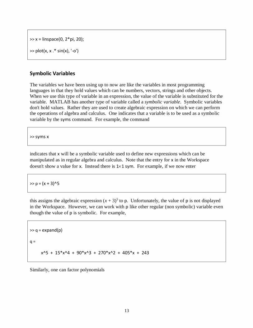
>> x = linspace(0, 2*pi, 20);

>> plot(x, x .* sin(x), '-o')

Symbolic Variables

The variables we have been using up to now are like the variables in most programming

languages in that they hold values which can be numbers, vectors, strings and other objects.

When we use this type of variable in an expression, the value of the variable is substituted for the

variable. MATLAB has another type of variable called a symbolic variable. Symbolic variables

don't hold values. Rather they are used to create algebraic expression on which we can perform

the operations of algebra and calculus. One indicates that a variable is to be used as a symbolic

variable by the syms command. For example, the command

>> syms x

indicates that x will be a symbolic variable used to define new expressions which can be

manipulated as in regular algebra and calculus. Note that the entry for x in the Workspace

doesn't show a value for x. Instead there is 11 sym. For example, if we now enter

>> p = (x + 3)^5

this assigns the algebraic expression (x + 3)5 to p. Unfortunately, the value of p is not displayed

in the Workspace. However, we can work with p like other regular (non symbolic) variable even

though the value of p is symbolic. For example,

>> q = expand(p) q =

x^5 + 15*x^4 + 90*x^3 + 270*x^2 + 405*x + 243

Similarly, one can factor polynomials

14

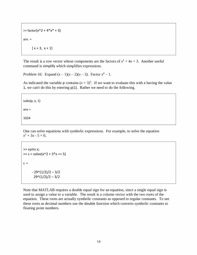
>> factor(x^2 + 4*x* + 3) ans =

[ x + 3, x + 1]

The result is a row vector whose components are the factors of x2 + 4x + 3. Another useful

command is simplify which simplifies expressions.

Problem 16: Expand (x – 1)(x – 2)(x – 3). Factor x4 – 1.

As indicated the variable p contains (x + 3)5. If we want to evaluate this with x having the value

1, we can't do this by entering p(1). Rather we need to do the following.

subs(p, x, 1) ans = 1024

One can solve equations with symbolic expressions. For example, to solve the equation

x2 + 3x - 5 = 0,

>> syms x; >> s = solve(x^2 + 3*x == 5) s =

- 29^(1/2)/2 – 3/2 29^(1/2)/2 – 3/2

Note that MATLAB requires a double equal sign for an equation, since a single equal sign is

used to assign a value to a variable. The result is a column vector with the two roots of the

equation. These roots are actually symbolic constants as opposed to regular constants. To see

these roots as decimal numbers use the double function which converts symbolic constants to

floating point numbers.

15

>> double(s) ans =

- 4.1926 1.1926

Problem 17: What is the Fahrenheit temperature when the Celsius temperature is 25 C? Use

solve. Recall C = 5

9 (F – 32).

Problem 18: Find the quotient of the larger root divided by the smaller root of the equation

x2 = 5x - 6. Express answer as a decimal.

Just as with human beings, MATLAB's ability to solve equations symbolically is rather limited.

For example, it can't do much with the following cubic.

>> solve(x^3 - 2 == x) ans =

root(x^3 – x – 2, x, 1) root(x^3 – x – 2, x, 2) root(x^3 – x – 2, x, 3)

In a case like this we can try the numeric solver:

>> vpasolve(x^3 - 2 == x) ans = 1.52138 - 0.76069 - 0.85787 i - 0.76069 - 0.85787 i

vpasolve gives all solutions to a polynomial equation.

Problem 19: Find the solutions of the equation x5 = 1 - x.

16

For non-polynomial equations, it is often necessary to specify an initial guess. For example, the

following command numerically finds an approximation to the equation sin x = x2 using 1 as an

initial guess.

>> vpasolve(sin(x) == x^2, x, 1) ans = 0.87673

What happens if you omit the 1?

Problem 20: Find the solution of xex = 1.

The diff command takes the derivative of symbolic expressions. Here is the first and second

derivative of ex2.

>> syms x >> diff(exp(x^2), x) ans = 2*x*exp(x^2) >> diff(exp(x^2),x,2) ans = 2*exp(x^2) + 4*x^2*exp(x^2)

Problem 21: Find the derivative of y = x

x2 - 1 .

The int command finds the integral of symbolic expressions. Here are xex dx and 1

2

xex dx.

17

>> int(x *exp(x), x) ans = exp(x) * (x – 1)

>> int(x *exp(x), x, 1, 2) ans = exp(2)

Problem 22: Find x

x2 - 1 dx and

2

3

x

x2 - 1 dx.

Whether or not a variable is a regular variable holding a value or a symbolic variable which is

used to create algebraic expressions can change according to the sequence of commands. Try the

following sequence of commands.

>> x = 3 >> y = x^2 >> syms x >> z = x^2 >> x = 4 >> u = x^2

After x = 3 is executed the variable x is a regular variable holding the value 3. So when y = x^2 is

executed, the value 3 is retrieved for x and 9 is stored in y. Then when syms x is executed, x

becomes a symbolic variable and the value 3 stored in it is lost. So when z = x^2 is executed the

algebraic expression x^2 is stored in z. Then when x = 4 is executed the variable x reverts back to

a regular variable holding the value 4. So when u = x^2 is executed, the value 4 is retrieved for x

and 16 is stored in u.

Live Scripts

So far, we have seen how to execute commands in the Command Window. There is an

alternative that is more convenient in many ways. For example, it is easier when one is

correcting errors or when one needs to execute a series of commands or one expects to

18

repeatedly use and modify several commands. Live Scripts allow one to write and save these

commands. Live Script files are created and edited using the MATLAB editor.

Let's write a Live Script that finds the volume and surface area of a cylinder of radius r and

height h. We shall use the formulas V = r2h and A = 2r2 + 2rh.

We begin by clicking on New on the tool bar and selecting Live Script on the drop down menu.

The Editor Window will appear, with a tab named Untitled.mlx.

In the editor window, type the following

r = 2; h = 3; V = pi*r^2*h A = 2*pi*r^2 + 2*pi*r*h

Note that there are no command prompts in the script window.

Click on the Live Editor tab on the menu bar and click Save. A box opens up for us to name the

file. Let's name it cylinder. Fill this in and click the Save button in the box. Note that the name

of the tab has been changed to cylinder.mlx and a file named cylinder.mlx appears in the Current

Folder Window.

To run the commands in the script, enter Ctrl-Enter (hold down the Ctrl key and press Enter). In

the editor window to the right of the commands one sees

V = 37.6991 A = 62.8319

If one has made an error, one simply corrects the error in the Editor window and enters Ctrl-

Enter again to re-execute the commands.

One can also enter comment lines in a Live Script by positioning the cursor where the comment

line is to go, clicking on the Live Editor tab on menu bar and clicking the Text button. A new

line opens up on which one can enter comments. To switch from comment lines to command

lines, click the Code button.

I encourage you to use Live Scripts for your work instead of the Command Window.

As noted above, the Current Folder Window contains the contents of the currently active folder

where files will be saved if one doesn't specify otherwise. The name of the Current Folder is

displayed above this Window and can be changed by using the back arrow to get to the root

folder of the desired folder and then going down to the desired folder. Often, the Current Folder

starts out as one titled MATLAB which is located inside Documents.

19

In the Mac lab in 2048 CB the folder MATLAB inside Documents is a temporary folder that

disappears when you Logoff. You should save items in that folder that you want to keep either

on a flash drive or in your campus file space before you Logoff. To get to your campus file

space, use the Fetch program which is in the Applications folder. Enter login-umd.umich.edu in

the Hostname field, your campus id in the Username field and your password in the Password

field. Click Connect. Your campus file space should appear. You can drag files back and forth

between your campus file space and folder on the Mac.

Whether or not the Workspace Window, the Current Folder Window and the Command History

Window are displayed can be controlled using the Layout or Preferences options in the

Environment menu.