Math 3070 § 1.Treibergs

Probability Plots for Normal,Exponential and Weibull Variables

Name: ExampleOctober 7, 2010

Data File Used in this Analysis:

# M3070 - 1 Geyser Data Oct. 7, 2010# Data from Navidi, "Principles of Statistics for Engineers and Scientists"# McGraw Hill, 2010# The following are durations in minutes of 40 consecutive time intervals# between eruptions of the Old Faithful geyser in Yellowstone National Park#Dormant91517953825176828453865185458851804982757367688672757566847079608671678176837655

1

R Session:

R version 2.10.1 (2009-12-14)Copyright (C) 2009 The R Foundation for Statistical ComputingISBN 3-900051-07-0

R is free software and comes with ABSOLUTELY NO WARRANTY.You are welcome to redistribute it under certain conditions.Type ’license()’ or ’licence()’ for distribution details.

Natural language support but running in an English locale

R is a collaborative project with many contributors.Type ’contributors()’ for more information and’citation()’ on how to cite R or R packages in publications.

Type ’demo()’ for some demos, ’help()’ for on-line help, or’help.start()’ for an HTML browser interface to help.Type ’q()’ to quit R.

[R.app GUI 1.31 (5538) powerpc-apple-darwin8.11.1]

[Workspace restored from /Users/andrejstreibergs/.RData]

> # Description of automated probability plot may be found in> help(qqnorm)

> # SOME DATA IS CANNED IN R.> # precip HAS ANNUAL RAINFALL OF 70 US CITIES (IN INCHES)> precip

Mobile Juneau Phoenix67.0 54.7 7.0

Little Rock Los Angeles Sacramento48.5 14.0 17.2

San Francisco Denver Hartford20.7 13.0 43.4

Wilmington Washington Jacksonville40.2 38.9 54.5Miami Atlanta Honolulu59.8 48.3 22.9Boise Chicago Peoria11.5 34.4 35.1

Indianapolis Des Moines Wichita38.7 30.8 30.6

Louisville New Orleans Portland43.1 56.8 40.8

Baltimore Boston Detroit41.8 42.5 31.0

Sault Ste. Marie Duluth Minneapolis/St Paul31.7 30.2 25.9

Jackson Kansas City St Louis

2

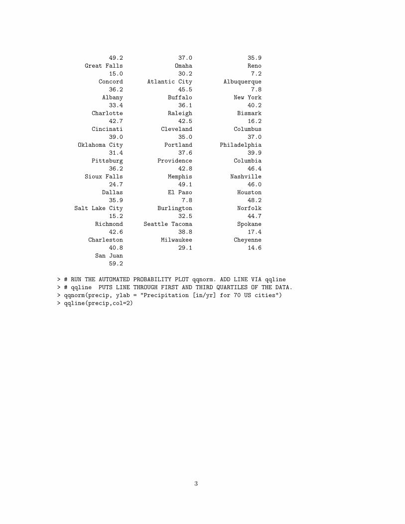
49.2 37.0 35.9Great Falls Omaha Reno

15.0 30.2 7.2Concord Atlantic City Albuquerque

36.2 45.5 7.8Albany Buffalo New York33.4 36.1 40.2

Charlotte Raleigh Bismark42.7 42.5 16.2

Cincinati Cleveland Columbus39.0 35.0 37.0

Oklahoma City Portland Philadelphia31.4 37.6 39.9

Pittsburg Providence Columbia36.2 42.8 46.4

Sioux Falls Memphis Nashville24.7 49.1 46.0

Dallas El Paso Houston35.9 7.8 48.2

Salt Lake City Burlington Norfolk15.2 32.5 44.7

Richmond Seattle Tacoma Spokane42.6 38.8 17.4

Charleston Milwaukee Cheyenne40.8 29.1 14.6

San Juan59.2

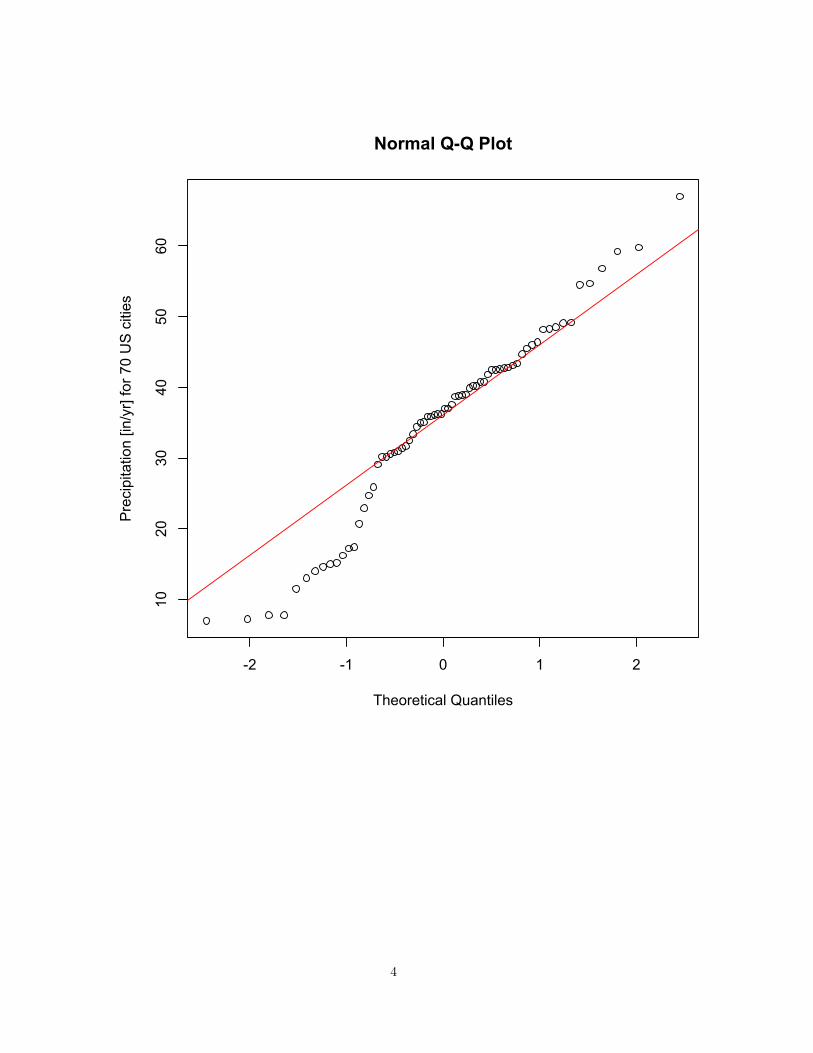
> # RUN THE AUTOMATED PROBABILITY PLOT qqnorm. ADD LINE VIA qqline> # qqline PUTS LINE THROUGH FIRST AND THIRD QUARTILES OF THE DATA.> qqnorm(precip, ylab = "Precipitation [in/yr] for 70 US cities")> qqline(precip,col=2)

3

-2 -1 0 1 2

1020

3040

5060

Normal Q-Q Plot

Theoretical Quantiles

Pre

cipi

tatio

n [in

/yr]

for 7

0 U

S c

ities

4

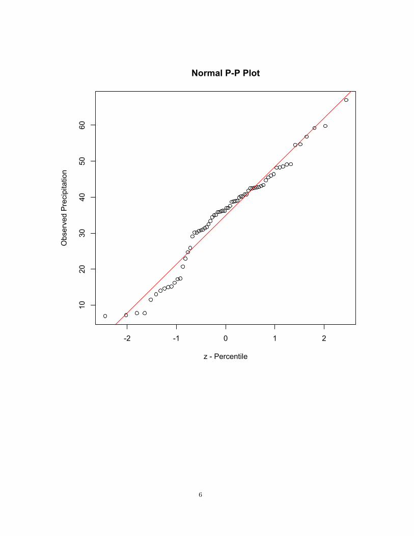
> ########################################################################> # DO THE PP PLOT BY HAND. GET SIZE OF SAMPLE> n <- length(precip)

> # GET FRACTIONS (PERCENTILES) OF THE OBSERVED SAMPLE.> Fi <- (1:70-0.5)/70> Fi[1] 0.007142857 0.021428571 0.035714286 0.050000000 0.064285714 0.078571429[7] 0.092857143 0.107142857 0.121428571 0.135714286 0.150000000 0.164285714

[13] 0.178571429 0.192857143 0.207142857 0.221428571 0.235714286 0.250000000[19] 0.264285714 0.278571429 0.292857143 0.307142857 0.321428571 0.335714286[25] 0.350000000 0.364285714 0.378571429 0.392857143 0.407142857 0.421428571[31] 0.435714286 0.450000000 0.464285714 0.478571429 0.492857143 0.507142857[37] 0.521428571 0.535714286 0.550000000 0.564285714 0.578571429 0.592857143[43] 0.607142857 0.621428571 0.635714286 0.650000000 0.664285714 0.678571429[49] 0.692857143 0.707142857 0.721428571 0.735714286 0.750000000 0.764285714[55] 0.778571429 0.792857143 0.807142857 0.821428571 0.835714286 0.850000000[61] 0.864285714 0.878571429 0.892857143 0.907142857 0.921428571 0.935714286[67] 0.950000000 0.964285714 0.978571429 0.992857143

> # GET THE CORRESPONDING z - scores BY SOLVING Fi = Phi(Zi).> Zi <- qnorm(Fi,0,1)> Zi[1] -2.44999766 -2.02509955 -1.80274309 -1.64485363 -1.51975951 -1.41474643[7] -1.32336422 -1.24186679 -1.16787512 -1.09977866 -1.03643339 -0.97699540

[13] -0.92082298 -0.86741569 -0.81637496 -0.76737743 -0.72015662 -0.67448975[19] -0.63018825 -0.58709060 -0.54505704 -0.50396537 -0.46370775 -0.42418819[25] -0.38532047 -0.34702648 -0.30923489 -0.27188001 -0.23490082 -0.19824019[31] -0.16184417 -0.12566135 -0.08964235 -0.05373932 -0.01790544 0.01790544[37] 0.05373932 0.08964235 0.12566135 0.16184417 0.19824019 0.23490082[43] 0.27188001 0.30923489 0.34702648 0.38532047 0.42418819 0.46370775[49] 0.50396537 0.54505704 0.58709060 0.63018825 0.67448975 0.72015662[55] 0.76737743 0.81637496 0.86741569 0.92082298 0.97699540 1.03643339[61] 1.09977866 1.16787512 1.24186679 1.32336422 1.41474643 1.51975951[67] 1.64485363 1.80274309 2.02509955 2.44999766

> # PUT THE OBSERVATIONS INTO INCREASING ORDER.> # PLOT SP VS. Zi. DRAW THE BEST FIT LINE THIS TIME.> SP <- sort(precip)> plot(Zi,SP,ylab="Observed Precipitation",xlab="z - Percentile",main="Normal P-P Plot")> abline(lm(SP~Zi),col=2)

5

-2 -1 0 1 2

1020

3040

5060

Normal P-P Plot

z - Percentile

Obs

erve

d P

reci

pita

tion

6

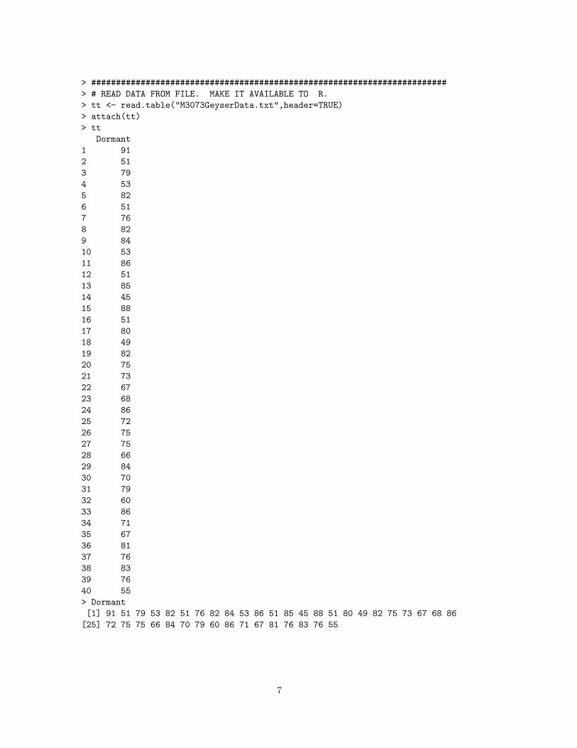
> ########################################################################> # READ DATA FROM FILE. MAKE IT AVAILABLE TO R.> tt <- read.table("M3073GeyserData.txt",header=TRUE)> attach(tt)> tt

Dormant1 912 513 794 535 826 517 768 829 8410 5311 8612 5113 8514 4515 8816 5117 8018 4919 8220 7521 7322 6723 6824 8625 7226 7527 7528 6629 8430 7031 7932 6033 8634 7135 6736 8137 7638 8339 7640 55> Dormant[1] 91 51 79 53 82 51 76 82 84 53 86 51 85 45 88 51 80 49 82 75 73 67 68 86

[25] 72 75 75 66 84 70 79 60 86 71 67 81 76 83 76 55

7

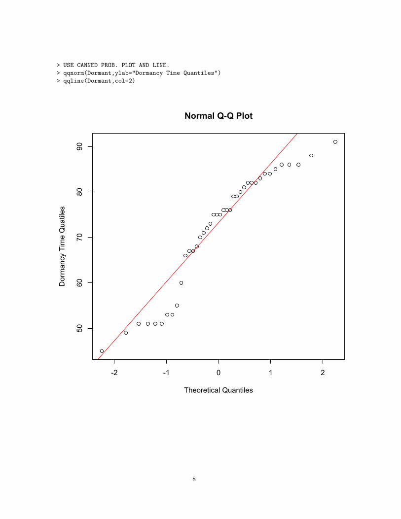
> USE CANNED PROB. PLOT AND LINE.> qqnorm(Dormant,ylab="Dormancy Time Quantiles")> qqline(Dormant,col=2)

-2 -1 0 1 2

5060

7080

90

Normal Q-Q Plot

Theoretical Quantiles

Dor

man

cy T

ime

Qua

tiles

8

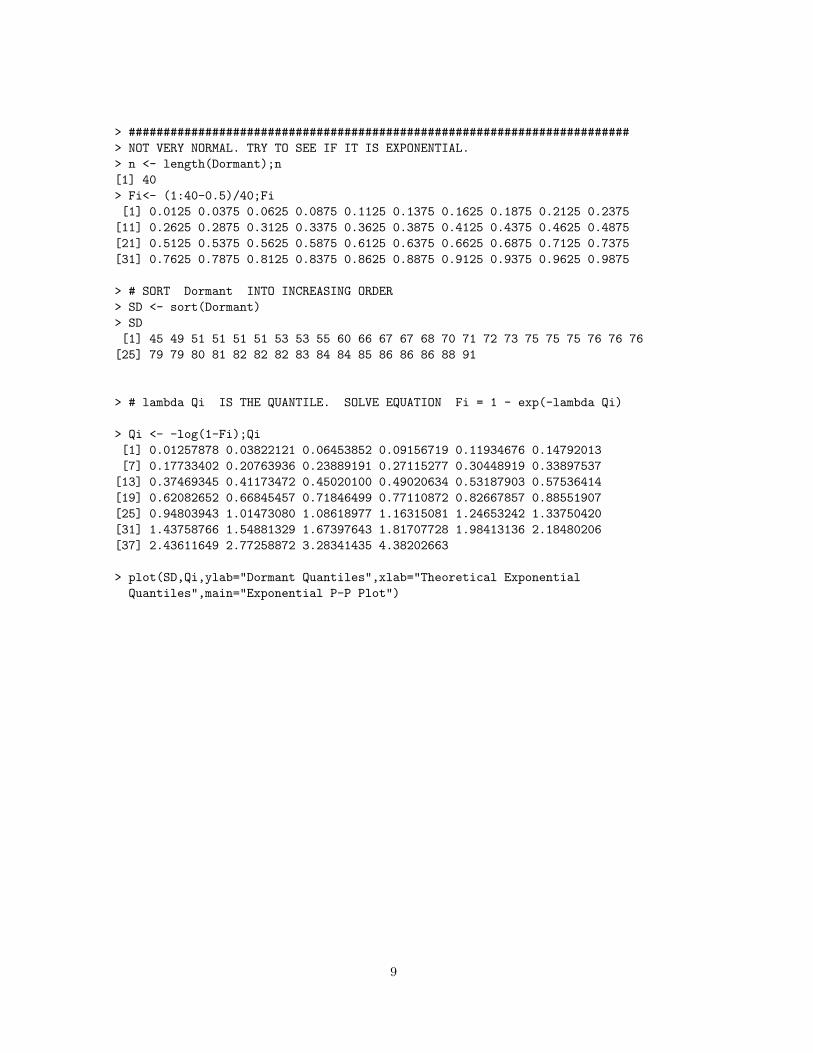
> ########################################################################> NOT VERY NORMAL. TRY TO SEE IF IT IS EXPONENTIAL.> n <- length(Dormant);n[1] 40> Fi<- (1:40-0.5)/40;Fi[1] 0.0125 0.0375 0.0625 0.0875 0.1125 0.1375 0.1625 0.1875 0.2125 0.2375

[11] 0.2625 0.2875 0.3125 0.3375 0.3625 0.3875 0.4125 0.4375 0.4625 0.4875[21] 0.5125 0.5375 0.5625 0.5875 0.6125 0.6375 0.6625 0.6875 0.7125 0.7375[31] 0.7625 0.7875 0.8125 0.8375 0.8625 0.8875 0.9125 0.9375 0.9625 0.9875

> # SORT Dormant INTO INCREASING ORDER> SD <- sort(Dormant)> SD[1] 45 49 51 51 51 51 53 53 55 60 66 67 67 68 70 71 72 73 75 75 75 76 76 76

[25] 79 79 80 81 82 82 82 83 84 84 85 86 86 86 88 91

> # lambda Qi IS THE QUANTILE. SOLVE EQUATION Fi = 1 - exp(-lambda Qi)

> Qi <- -log(1-Fi);Qi[1] 0.01257878 0.03822121 0.06453852 0.09156719 0.11934676 0.14792013[7] 0.17733402 0.20763936 0.23889191 0.27115277 0.30448919 0.33897537

[13] 0.37469345 0.41173472 0.45020100 0.49020634 0.53187903 0.57536414[19] 0.62082652 0.66845457 0.71846499 0.77110872 0.82667857 0.88551907[25] 0.94803943 1.01473080 1.08618977 1.16315081 1.24653242 1.33750420[31] 1.43758766 1.54881329 1.67397643 1.81707728 1.98413136 2.18480206[37] 2.43611649 2.77258872 3.28341435 4.38202663

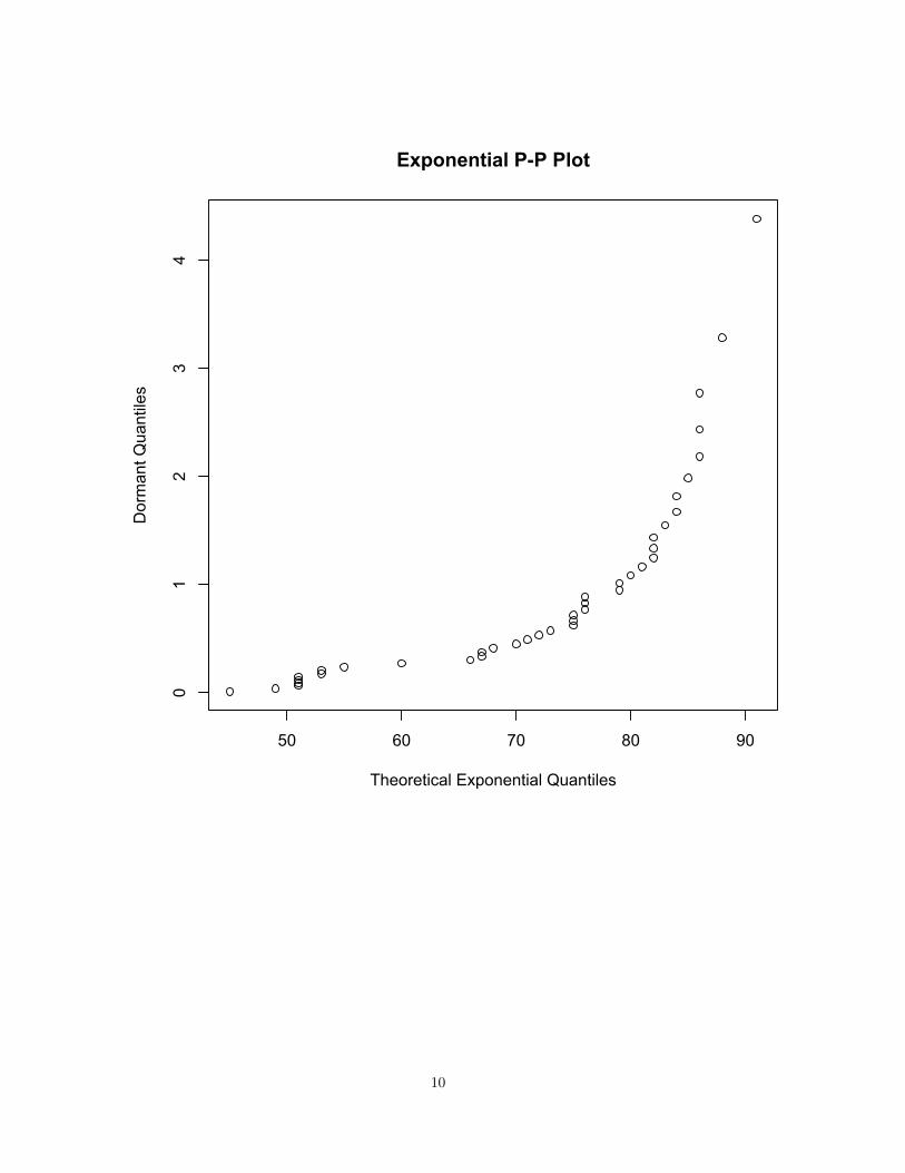
> plot(SD,Qi,ylab="Dormant Quantiles",xlab="Theoretical ExponentialQuantiles",main="Exponential P-P Plot")

9

50 60 70 80 90

01

23

4Exponential P-P Plot

Theoretical Exponential Quantiles

Dor

man

t Qua

ntile

s

10

> ########################################################################> # QUITE BOWED SO NOT EXPONENTIAL. TRY WEIBULL USING METHOD IN TEXT.

> # Qi/bets IS THE QUANTILE. SOLVE EQUATION Fi = 1 - exp(-(-Qi/beta )^alpha)> Eta <- log(-log(1-Fi))

> plot(Eta,log(SD),ylab="Log Dormant Quantiles",xlab="Theoretical Weibull Quantiles",main="Weibull P-P Plot")

> # ADD LINE. WORK OUT SLOPE m AND INTCPT b FROM 4th TO 37th POINT> m<- (log(SD[37])-log(SD[4]))/(Eta[37]-Eta[4]);m[1] 0.1592526> b <- log(SD[4])-m*Eta[4];b[1] 4.312548> abline(b,m,col=3)> # NOT SO WEIBULL EITHER, BUT SLIGHTLY "BETTER" THAN NORMAL OR EXPONENTIAL.

11

-4 -3 -2 -1 0 1

3.8

3.9

4.0

4.1

4.2

4.3

4.4

4.5

Weibull P-P Plot

Theoretical Weibull Quantiles

Log

Dor

man

t Qua

ntile

s

12