MATH 4512 — Fundamentals of Mathematical Finance

Topic One — Bond portfolio management and immunization

1.1 Duration measures and convexity

1.2 Horizon rate of return: return from the bond investment over a time

horizon

1.3 Immunization of bond investment

1.4 Optimal management and dynamic programming

1

1.1 Duration measures and convexity

Fixed coupon bond

Let i be the interest rate applicable to the cash flows arising from a fixed

coupon bond, giving constant coupon c paid at times 1,2, . . . , T and par

amount BT paid at maturity T .

The fair bond value B is the sum of the coupons and par in present value,

where

B =c

1+ i+ · · ·+

c

(1 + i)T+

BT

(1 + i)T

= c

1

1+ i

1− 1(1+i)T

1− 11+i

+BT

(1 + i)T=

c

i

[1−

1

(1 + i)T

]+

BT

(1 + i)T.

2

Annuity factor and present value factor

The discrete coupons paid at times 1,2, . . . , T is called an annuity stream

over the time period [0, T ]. We define the annuity factor (i, T ) to be

annuity factor (i, T ) =1

i

[1−

1

(1 + i)T

].

The present value factor over [0, T ] at interest rate i is defined by

PV factor (i, T ) =1

(1+ i)T.

• When T → ∞, the annuity factor becomes1

i. For example, when

i = 5%, one needs to put $20 upfront in order to generate a perpetual

stream of annuity of $1 paid annually.

• For an annuity of finite time horizon T , it can be visualized as the

difference of two perpetual annuities starting on today and time T .

The present value of the perpetual starting at time T is1

i

1

(1 + i)T.

3

Par bond

Suppose the coupon rate is set to be the interest rate so that the coupon

amount c = iBT , then

B =iBT

i

[1−

1

(1 + i)T

]+

BT

(1 + i)T= BT .

This is called a par bond, so named since the bond value is equal to

the par of the bond. Obviously, if the coupon rate is above (below) the

discount rate, then the bond value B is above (below) the par value BT .

Yield to maturity

Yield to maturity (YTM) of a bond is the rate of return anticipated on a

bond if held until maturity. The yield to maturity is determined by finding

the rate of return of the bond such that the sum of cash flows discounted

at the rate of return is equal to the observed bond price. Here, the value

of B is given, we find YTM i.

4

Duration

The duration of a bond is the weighted average of the times of pay-

ment of all the cash flows generated by the bond, the weights being the

proportional shares of the bond’s cash flows in the bond’s present value.

Macauley’s duration:

Let i denote the yield to maturity (YTM) of the bond. Bond duration is

D = 1c/B

1+ i+2

c/B

(1 + i)2+ · · ·+ T

(c+BT )/B

(1 + i)T

=1

B

T∑t=1

tct

(1 + i)t. (D1)

where ct is the cash flow at time t. Note that cT = c+BT .

5

Measure of a bond’s sensitivity to change in interest rate

Starting from

B =T∑

t=1

ct(1 + i)−t,

dB

di=

T∑t=1

(−t)ct(1 + i)−t−1 = −1

1+ i

T∑t=1

tct(1 + i)−t;

1

B

dB

di= −

1

1+ i

T∑t=1

tct(1 + i)−t

B= −

D

1+ i.

Modified duration = Dm = duration1+i

∆B

B≈

dB

B= −Dm di and var

(dB

B

)= D2

mvar(di).

The standard deviation of the relative change in the bond price is a linear

function of the standard deviation of the changes in interest rates, the

coefficient of proportionality is the modified duration.

6

Suppose a bond is at par, its coupon is 9%, so YTM = 9%. The duration

is found to be 6.99. Suppose that the interest rate (yield) increases by

1%, then the relative change in bond value is

∆B

B≈

dB

B= −

D

1+ idi = −

6.99

1.09× 1% = −6.4%.

How good is the linear approximation? For exact calculation, we have

∆B

B=

B(10%)−B(9%)

B(9%)=

93.855− 100

100= −6.145%.

Later, we show how to obtain the quadratic approximation (an improve-

ment over the linear approximation) with the inclusion of convexity (re-

lated tod2B

di2).

7

Example

A bond with annual coupon 70, par 1000, and interest rate 5%; duration

is found to be 7.7 years, modified duration = 7.71.05 = 7.33 yr.

A change in yield from 5% to 6% or 4% entails a relative change in the

bond price approximately −7.33% or +7.33%, respectively. The modified

duration is seen to be the more appropriate proportional factor.

8

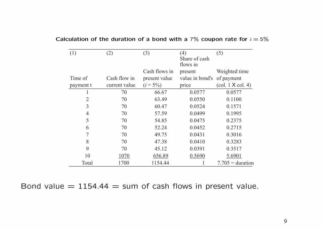
Calculation of the duration of a bond with a 7% coupon rate for i = 5%

(1) (2) (3) (4) (5)

Time of

payment t

Cash flow in

current value

Cash flows in

present value

( = 5%)i

Share of cashflows in

present

value in bond's

price

Weighted time

of payment

(col. 1 col. 4)X

1 70 66.67 0.0577 0.0577

2 70 63.49 0.0550 0.1100

3 70 60.47 0.0524 0.1571

4 70 57.59 0.0499 0.1995

5 70 54.85 0.0475 0.2375

6 70 52.24 0.0452 0.2715

7 70 49.75 0.0431 0.3016

8 70 47.38 0.0410 0.3283

9 70 45.12 0.0391 0.3517

10 1070 656.89 0.5690 5.6901

Total 1700 1154.44 7.705 = duration1

Bond value = 1154.44 = sum of cash flows in present value.

9

Duration of a bond as the center of gravity of its cash flows in present

value (coupon: 7%; interest rate: 5%).

10

Duration in terms of coupon rate, maturity and interest rate

Recall B = ci

[1− 1

(1+i)T

]+ BT

(1+i)T. We express

B

BTin terms of

c

BT, i and

T as

B

BT=

1

i

{c

BT

[1−

1

(1 + i)T

]+

i

(1 + i)T

}.

d ln(

BBT

)di

=d lnB

di=

1

B

dB

di

= −1

i+

(c/BT )T (1 + i)−T−1 + (1+ i)−T + i(1 + i)−T−1(−T )

(c/BT )[1− (1 + i)−T ] + i(1 + i)−T

so that the duration D is related to c/BT , i and T as

D = −1+ i

B

dB

di= 1+

1

i+

T(i− c

BT

)− (1 + i)

cBT

[(1 + i)T − 1] + i. (D2)

• The impact of the coupon rate c/BT and maturity T for a fixed value

of i on duration D can be deduced from the last term.

11

Term structure of duration

• Obviously, D = T when c = 0 since there is only one cash flow of par

paid at maturity T .

Duration of a bond as a function of its maturity for various coupon rates

(i = 10%).

12

Note that the numerator = T(i− c

BT

)− (1 + i) is a linear function in T .

When the coupon rate cBT

is less than i, the numerator may change sign

at T ∗ where

T ∗(i−

c

BT

)= 1+ i.

That is, D may assume value above 1 + 1i when T > T ∗. When c

BT> i,

the numerator is always negative so D always stays below 1+ 1i .

13

Impact of coupon rate on duration

With an increase in the coupon rate c/BT , should there always be a

decrease in duration for sure?

• From eq. (D2), it is seen that the numerator (denominator) in the

last term decreases (increases) with increasing c/BT . Hence, D always

decreases with increasing c/BT .

• Intuitively, when the coupon rate increases, the weights will be tilted

towards the left, and the center of gravity will move to the left.

14

Perpetual bond – infinite maturity (T → ∞)

• For a perpetual bond, B = c/i. The modified duration D∗ is −1

B

dB

di=

c

i2

/c

i=

1

i. This gives D =

1+ i

i= 1+

1

i.

• Alternatively, we observe from eq.(D2) on P.11 that

limT→∞

T(i− c

BT

)− (1 + i)

cBT

[(1 + i)T − 1] + i= 0.

This leads to

D → 1+1

ias T → ∞. (D3)

When i = 10%, we have D → 11 as T → ∞.

In Qn 1 of HW 1, when there are m compounding periods in one year,

we have D → 1m + 1

i as T → ∞. When m → ∞, which corresponds to

continuous compounding, we obtain

D →1

ias T → ∞.

15

Relationship between duration and maturity

1. For zero-coupon bonds, duration is always equal to maturity.

For all coupon-bearing bonds, we observe

duration → 1+ 1i when maturity increases infinitely.

The limit is independent of the coupon rate.

2. Coupon rate ≥ interest rate (bonds above par)

An increase in maturity entails an increase in duration towards the

limit 1 + 1i .

3. Coupon rate < interest rate (bonds below par)

When maturity increases, duration first increases, pass through a max-

imum and decreases toward the limit 1 + 1i .

16

Change of duration with respect to change in interest rate

Intuitively, since the discount factor for the cash flow at time t is (1+i)−t,

an increase in i will move the center of gravity to the left, and the duration

is reduced. Actually

dD

di= −

S

1+ i,

where S is the dispersion or weighted variance of the payment times of

the bond. The respective weight is the present value of the cash flow at

the corresponding payment time.

17

Proof

Starting from

D =1

B

T∑t=1

tct(1 + i)−t

dD

di= −

1

B2

T∑t=1

t2ct(1 + i)−t−1B(i) +T∑

t=1

tct(1 + i)−tB′(i)

= −1

1+ i

T∑

t=1

t2ct(1 + i)−t

B(i)+ (1+ i)

B′(i)

B(i)︸ ︷︷ ︸−D

∑Tt=1 tct(1 + i)−t

B(i)︸ ︷︷ ︸D

= −

1

1+ i

[∑Tt=1 t

2ct(1 + i)−t

B(i)−D2

].

18

If we write

wt =ct(1 + i)−t

B(i)

so thatT∑

t=1

wt = 1 and D =T∑

t=1

twt.

Here, wt is the share of the bond’s cash flow ct (in the present value) in

the bond’s value. The bracket term becomes

T∑t=1

t2wt −D2 =T∑

t=1

wt(t−D)2,

which is equal to the weighted average of the squares of the difference

between the times t and their average D.

We obtain

dD

di= −

1

1+ i

T∑t=1

wt(t−D)2 = −S

1+ i,

which is always negative.

19

Fair holding-period return

To illustrate built-in capital gains or losses, suppose a bond was issued

several years ago when the interest rate was 7%. Suppose the bond was

sold at par, then the bond’s annual coupon rate was thus set at 7%. Let

the par value be $1,000.

We will suppose for simplicity that the bond pays its coupon annually.

Now, with 3 years left in the bond’s life, the interest rate is 8% per year.

The bond’s market price is the present value of the remaining annual

coupons plus payment of par value. That present value is

$70×Annuity factor(8%,3) + $1,000× PV factor(8%,3) = $974.23

which is less than par value.

One year later, after the next coupon is paid, the bond would sell at

$70×Annuity factor(8%,2) + $1,000× PV factor(8%,2) = $982.17

thereby yielding a capital gain over the year of $982.17−$974.23 = $7.94.

20

An increase in bond value after one year is expected since the disadvantage

of receiving coupon at the rate of 7% while the interest rate is 8% is

diminished with the passage of one year.

If an investor had purchased the bond at $974.23, the total return over the

year would equal the coupon payment plus capital gain, or $70+$7.94 =

$77.94. This represents a rate of return of $77.94/$974.23, or 8%, exactly

the current rate of return available elsewhere in the market.

In an efficient financial market, the rate of return of holding bonds with

different coupon rates would be the same. We have neglected default risk

and liquidity risk that are typical in bonds investment. Mathematically,

we have

i =c

B+

∆B

B.

Here, c/B is called the direct rate of return of the bond (not to be

confused with the coupon rate c/BT ).

21

Mystery behind duration

Recall that suppose the constant interest rate r is compounded contin-

uously over [0, T ], then the growth factor is erT . This arises from the

solution to the differential equation for the money market account M ,

where

dM = rMdt, M(0) = 1.

Observe that ∫ T

0

dM

M=

∫ T

0r dt

lnM(T )

M(0)= rT

so that

M(T ) = erT .

Here, erT is visualized as the growth factor of a fund over [0, T ]. The

reciprocal of the growth factor, namely e−rT , is called the discount factor.

22

Under the continuous framework, the bond value B(⃗i) is given by

B(⃗i) =∫ T

0c(t)e−i(0,t)t dt,

where c(t) is the cash flow rate received at time t and i(0, t) is the t-year

spot rate compounded continuously over the interval (0, t). For a given

value t, i(0, t) is the corresponding spot rate applicable for the cash flow

amount c(t)dt over (t, t+dt) known at time zero. Therefore, the discount

factor is e−i(0,t)t. This is considered as a functional since this is a relation

between a function i⃗ (term structure of the spot rates) and a number

B(⃗i).

Naturally, duration of the bond with the initial term structure of the spot

rate as characterized by i(0, t) is given by

D(⃗i) =1

B(⃗i)

∫ T

0tc(t)e−i(0,t)t dt,

where c(t)e−i(0,t)t

B(⃗i)dt represents the weighted present value of the cash flow

within (t, t+ dt). We would like to understand the financial intuition why

duration is the multiplier that relates relative change in bond value and

interest rate.23

Suppose the whole term structure of spot rates move up in parallel shift

by ∆α, then

B(⃗i+∆α) =∫ T

0c(t)e−i(0,t)te−t∆α dt.

Note that when ∆α is infinitesimally small, we have

e−t∆α ≈ 1− t∆α

so that the discounted cash flow e−i(0,t)tc(t) dt within (t, t+dt) decreases in

proportional amount t∆α. The corresponding contribution to the relative

change in bond value as normalized by B(⃗i) is

−tc(t)e−i(0,t)t dt

B(⃗i)∆α.

Note the role of the term −t∆α, involving (−t), which contributes to the

relative change of the bond value.

24

This is the payment time t weighted by the discounted cash flowc(t)dt

B(i)e−i(0,t)t

within (t, t+ dt) multiplied by the change in interest rate ∆α. Therefore,

we have

B(⃗i+∆α)−B(⃗i)

B(⃗i)≈ −∆α

∫ T

0

tc(t)e−i(0,t)t

B(⃗i)dt.

The relative change in bond value

∆B

B≈ −∆α

[weighted average of payment times that are

weighted according to present value of cash flow

]= −D∆α.

In the differential limit,B(⃗i+∆α)−B(⃗i)

B(⃗i)becomes

dB

Band ∆α is identi-

fied as the differential dα, so we obtain

dB

B= −D(⃗i) dα.

25

Special case: discount bond (zero coupon bearing)

Since there is only one par payment P in a discount bond that is paid at

T years, then

dBdis

di=

d

di

[P

(1 + i)T

]= −

T

1+ iBdis = −

D

1+ iBdis,

where i is the interest rate per annum and D = T .

If the interest rate is compounded m times per year, then

dBdis

di=

d

di

P

(1 + im)mT

= −T

1+ im

Bdis = −D

1+ im

Bdis,

As m → ∞, which corresponds to continuous compounding, we obtain

dBdis

Bdis= −D di.

The factor 11+i disappears in continuous compounding.

26

Summary of formulas for continuous bond models

• Value of a bond in continuous time, with i⃗ = i(0, t) being the term

structure of spot rates:

B(⃗i) =∫ T

0c(t)e−i(0,t)t dt

• Duration of the bond:

D(⃗i) =1

B(⃗i)

∫ T

0tc(t)e−i(0,t)t dt

• Duration of the bond when i⃗ receives a (constant) drift α:

D(⃗i+ α) =1

B(⃗i+ α)

∫ T

0tc(t)e−[i(0,t)+α]t dt

• Fundamental property of duration:

−1

B(⃗i)

dB(⃗i)

dα=

1

B(⃗i)

∫ T

0tc(t)e−i(0,t)t dt = D

27

1.2 Horizon rate of return: return from the bond investment over

a time horizon

Horizon rate of return, rH – bond is kept for a time horizon H

Suppose a bond investor bought a bond valued at B(i0) when the interest

rate common to all maturities was i0 (flat rate). On the following day,

the interest rate moves up to i (parallel shift). The new future value at

H given the bond price B(i) at the new interest rate level i is given by

B(i)(1 + i)H since the future cash flows from the bond are assumed to

be compounded annually at the new interest rate i (though H may not

be an integer). To the investor, by paying B0 as the initial investment,

the new horizon rate of return based on the new future value is given by

B0(1 + rH)H = B(i)(1 + i)H and so

rH =

[B(i)

B0

]1/H(1 + i)− 1.

The impact on the bond value on changing interest rate is spread out in

H years.

28

Example – Calculation of rH

A 10-year bond with coupon rate of 7% was bought when the interest

rates were at 5%. We have B(i0) = $1154.44.

Suppose on the next day, the interest rates move up to 6%. The bond

drops in value to $1073.60. If he holds his bond for 5 years (horizon is

chosen to be 5 years), and if interest rates stay at 6%, then

rH =(1073.60

1154.44

)1/5(1.06)− 1 = 4.47%.

Observation

Though the rate of interest at which the investor can reinvest his coupons

(which is now 6%) is higher, his overall performance will be lower than

5% (rH is only 4.47%).

29

• As a function of i, the horizon rate of return rH is a product of a

decreasing function B(i) and an increasing function (1 + i). This

represents a counterbalance between an immediate capital gain/loss

and rate of return based on new i on the cashflows from now till H.

• Whatever the horizon, the horizon rate of return will always be i0 if i

does not move away from this value. In this case,

FH = B0(1 + i0)H = B0(1 + rH)H

so that rH = i0 for any H (see the column in the table on the next

page under i = 5%).

• If H → ∞, then rH =[B(i)B0

]1/H(1 + i) − 1 → i. With infinite time

of horizon, the immediate change of bond price is immaterial. The

horizon rate of return is simply the new prevailing interest rate i.

30

The table shows the horizon rate of return (in percentage per year) on

the investment in a 7% coupon, 10-year maturity bond bought at 1154.44

when interest rates were at 5%, should interest rates move immediately

either to 6% or 4%. At H = 7.7, which is the duration of the bond, rHincreases when i either increases or decreases.

Horizon (years) 4% 5% 6%

1 12.01 5 -1.42

2 7.93 5 2.22

3 6.60 5 3.47

4 5.95 5 4.09

5 5.55 5 4.47

6 5.29 5 4.73

7 5.11 5 4.92

7.7 5.006 5 5.006

8 4.97 5 5.04

9 4.86 5 5.15

10 4.77 5 5.23

4.00 6.00

Interest rates

Hr

increasing

31

• Comparing the one-year horizon and four-year horizon, if interest rates

rise (see the last column in the previous table under i = 6%), the four-

year horizon return is higher than the one-year horizon return. This

is because the longer the horizon and the longer the reinvestment of

the coupons at a higher rate, the greater the chance that the investor

will outperform the initial yield of 5%.

• The duration of the 10-year 7%-coupon rate bond is found to be 7.7

years. When the horizon is chosen to be 7.7 years, then the horizon

rate of return will be slightly above 5% (5.006%) whether the interest

rate falls to 4% or increases to 6%.

• For the extreme case of H → ∞, rH = i. The immediate capital

gain/loss is immaterial since all cash flows from the bonds remain the

same while they can be reinvested at the rate of return i.

32

Example

An insurance company issues a guaranteed investment contract (GIC) for

$10,000. Essentially, GICs are zero-coupon bonds issued by the insurance

company to its customers. They are popular products for individuals’

retirement-savings accounts. If the GIC has a 5-year maturity and a

guaranteed interest rate of 8%, the insurance company promises to pay

$10,000× (1.08)5 = $14,693.28 in 5 years.

Suppose that the insurance company chooses to fund its obligation with

$10,000 of 8% annual coupon bonds, selling at par value, with 6 years to

maturity. It happens that this 8%-coupon bond with 6 years to maturity

has a duration that matches with the time horizon of 5 years. As long as

the market interest rate stays at 8%, the company has fully funded the

obligation, as the present value of the obligation exactly equals the value

of the bonds.

33

The following table shows that if interest rates remain at 8%, the accumu-

lated funds from the bond will grow to exactly the $14,693.28 obligation.

Over the 5-year period, year-end coupon income of $800 is reinvested

at the prevailing 8% market interest rate. At the end of the period, the

bonds can be sold for $10,000; they still will sell at par value because

the coupon rate still equals the market interest rate. Total income after

5 years from reinvested coupons and the sale of the bond is precisely

$14,693.28.

34

Price risk and reinvestment risk are offsetting

If interest rates change, two offsetting influences will affect the ability

of the fund to grow to the targeted value of $14,693.28. If interest

rate rise, the fund will suffer a capital loss, impairing its ability to satisfy

the obligation. The bonds will be worth less in 5 years than if interest

rates had remained at 8%. However, at a higher interest rate, reinvested

coupons will grow at a faster rate, offsetting the capital loss.

In other words, fixed-income investors face two offsetting types of interest

rate risk: price risk and reinvestment rate risk. Increases in interest rates

cause capital losses but at the same time increase the rate at which rein-

vested income will grow. If the portfolio duration is chosen appropriately,

these two effects will cancel out exactly.

35

When the portfolio duration is set equal to the investor’s horizon date,

the accumulated value of the investment fund at the horizon date will

be unaffected by interest rate fluctuations. For a horizon equal to the

portfolio’s duration, price risk and reinvestment risk exactly cancel out.

In this example, the duration of the 6-year maturity bonds used to fund

the GIC is 5 years. Since the fully funded plan has equal duration for

its assets and liabilities, the insurance company should be immunized

against interest rate fluctuations. To confirm this, we know that bond

can generate enough income to pay off the obligation in 5 years regardless

of interest rate movements.

36

37

• The horizon rate of return rH is a decreasing function of i when the

horizon H is short and an increasing one for long horizons. For a

horizon equal to the duration of the bond, the horizon rate of return

first decreases, goes through a minimum for i = i0 then increases by

i.

• There is a critical value for H such that rH changes from a decreasing

function of i to an increasing function of i. This critical value is the

bond duration. Why? Recall

∆B

B≈ −D ×∆i

• The immediate capital loss of amount D∆i is spread over H years.

• The gain in a higher rate of return of the future cash flows is H∆i

over H years of horizon of investment.

• These two effects are counterbalanced if H = D.

38

Dependence of rH on i with varying H

39

Remark

Suppose an investor is targeting at a time horizon of investment H, he

should choose a bond whose duration equals H so that the rate of return

at the target horizon is immunized from any change in the interest rate.

Stronger mathematical result

There exists a horizon H such that rH always increases when the inter-

est rate moves up or down from the initial value i0. The more precise

statement is stated in the following theorem.

Theorem

There exists a horizon H such that the rate of return for such a horizon

goes through a minimum at point i0.

40

Proof

Minimizing rH is equivalent to minimizing any positive function of it, and

so it is equivalent to minimizing B0(1 + rH)H = FH = B(i)(1 + i)H.

Consider

dFH

di=

d

di[B(i)(1 + i)H] = B′(i)(1 + i)H +HB(i)(1 + i)H−1,

we would like to find H such that the first order condition: dFHdi = 0 at

i = i0 is satisfied. This gives

B′(i0)(1 + i0) +HB(i0) = 0

andH = −

1+ i0B(i0)

B′(i0) = duration.

The horizon H must be chosen to be equal to the duration at the initial

rate of return i0 for FH to run through a minimum. If otherwise, thendFHdi = 0 at i = i0 cannot be satisfied. This is revealed by the other curves

(see P.39) that pass through i = i0, where they are either monotonic

increasing or decreasing in i.

41

Checking the second order condition

Recalld2 ln f

dx2=

f ′′f − f ′2

f2so

d2 ln f

dx2> 0 ⇒ f ′′ >

f ′2

f> 0 for f > 0. It

suffices to show that lnFH(i) = lnB(i)+H ln(1+ i) has a positive second

order derivative.

d lnFH

di=

d

dilnB(i) +

H

1+ i=

1

B(i)

dB(i)

di+

H

1+ i=

−D +H

1+ i

d2

di2lnFH =

1

(1+ i)2

[−dD

di(1 + i) +D −H

].

Setting H = D, we obtain

d2

di2lnFH = −

1

1+ i

dD

di=

S

(1 + i)2> 0.

Therefore, FH and rH go through a global minimum at point i = i0whenever H = D.

42

1.3 Immunization of bond investment

• In the case of either a drop or a rise in interest rates, when the horizon

was properly chosen, the horizon rate of return for the bond’s owner

was about the same as if interest rates had not moved. This horizon

is the duration of the bond.

• Immunization is the set of bond management procedures that aim at

protecting the investor against changes in interest rates.

• It is dynamic since the passage of time and changes in interest rates

will modify the portfolio’s duration by an amount that will not nec-

essarily correspond to the steady and natural decline of the investor’s

horizon.

43

• Even if interest rates do not change, the simple passage of one year

will reduce duration of the portfolio by less than one year. The money

manager will have to change the composition of the portfolio so that

the duration is reduced by a whole year. The new bond portfolio’s

duration is adjusted and targeted at the updated horizon.

• Changes in interest rates will also modify the portfolio’s duration.

• Immunization may be defined as the process by which an investor can

protect himself against interest rate changes by suitably choosing a

bond or a portfolio of bonds such that its duration is kept equal to

his horizon dynamically .

44

Duration matching and rebalancing

An insurance company must make a payment of $19,487 in seven years.

The market interest rate is 10%, so the present value of the obligation

is $10,000. The company’s portfolio manager wishes to fund the obliga-

tion using three-year zero-coupon bonds and perpetuities paying annual

coupons.

How can the manager immunize the obligation?

Immunization requires that the duration of the portfolio of assets equal

the duration of the liability. We can proceed in four steps:

Step 1. Calculate the duration of the liability. It is a single-payment

obligation with duration of seven years.

Step 2. Calculate the duration of the asset portfolio. The portfolio

duration is the weighted average of duration of each component asset,

with weights proportional to the funds placed in each asset.

45

• The duration of the zero-coupon bond is simply its maturity, three

years.

• The duration of the perpetuity is1

0.1+ 1 = 11 years.

If the fraction of the portfolio invested in the zero is called w, and the

fraction invested in the perpetuity is (1− w), then

asset duration = w × 3 years + (1− w)× 11 years

Step 3. Find the asset mix that sets the duration of assets equal to the

seven-year duration of liabilities. This requires us to solve for w in the

following equation

w × 3 years + (1− w)× 11 years = 7 years.

This gives w = 1/2.

46

Step 4. Fully fund the obligation. Since the obligation has a present

value of $10,000, and the fund will be invested equally in the zero and

the perpetuity, the manager must purchase $5,000 of the zero-coupon

bond and $5,000 of the perpetuity. Note that the face value of the

zero-coupon bond will be $5,000× (1.10)3 = $6,655.

Rebalancing

Suppose that one year has passed, and the interest rate remains at 10%.

The portfolio manager needs to reexamine her position.

Funding

The present value of the obligation will have grown to $11,000, as it is

one year closer to maturity. The manager’s funds also have grown to

$11,000: The zero-coupon bonds have increased in value from $5,000 to

$5,500 with the passage of time, while the perpetuity has paid its annual

$500 coupons and remains worth $5,000. Therefore, the obligation is

still fully funded since $11,000 = $5,500+ ($5,000+ $500).

47

The portfolio weights must be changed, however. The zero-coupon bond

now will have a duration of two years, while the perpetuity duration re-

mains at 11 years. The obligation is now due in six years. The weights

must now satisfy the equation

w × 2+ (1− w)× 11 = 6

which implies that w = 5/9.

To rebalance the portfolio and maintain the duration match, the manager

now must invest a total of $11,000×5/9 = $6,111.11 in the zero-coupon

bond. This indicates an increase of amount equals $6,111.11−$5,500 =

$611.11 in holding the zero-coupon bond. This requires that the entire

$500 coupon payment be invested in the zero, with an additional $111.11

of the perpetuity sold and invested in the zero-coupon bond.

48

Numerical example – matching duration

A company has an obligation to pay $1 million in 10 years. That is, the

future value at the time of horizon of 10 years is $1 million. It wishes

to invest money now that will be sufficient to meet this obligation. The

purchase of a single zero-coupon bond would provide one solution, but

such discount bonds are not always available in the required maturities.

coupon rate maturity price yield duration

bond 1 6% 30 yr 69.04 9% 11.44

bond 2 11% 10 yr 113.01 9% 6.54

bond 3 9% 20 yr 100.00 9% 9.61

• The above 3 bonds all have the yield of 9%. Present value of the

obligation of $1 million in 10 years at 9% yield is $414,643.

49

• Since bond 2 and bond 3 have their duration shorter than 10 years, it

is not possible to attain a portfolio with duration 10 years using these

two bonds. A bond with a longer maturity is required (say, bond 1)

to be included in the portfolio. The coupons received are reinvested

earning rate of return at the prevailing yield.

Suppose we use bond 1 and bond 2 of notional amount V1 and V2 in the

portfolio, by matching the present value and duration, we obtain

V1 + V2 = PV = $414,643D1V1 +D2V2

PV= 10

giving

V1 = $292,788.64 and V2 = $121,854.78.

Number of shares of bond 1 to be held is $292,798.64/$69.04 = 4,241,

which will be held fixed. Similarly, the number of bond 2 to be held is

$121,824.78/$113.01 = 1,078.

50

What would happen when we have a sudden change in the prevailing

yield?

• Obligation value at 8% yield = 1,000,000/(1.08)10 = 456,387.

• Surplus at 8% yield = 328,168.58+ 129,780.42− 456,386.95

= 1,562.05.

51

Observation

At different yields (8% and 10%), the value of the portfolio almost agrees

with that of obligation (at the new yield) with a small amount of surplus.

Difficulties in the implementation of immunization

• It is quite unrealistic to assume that both the long- and short-duration

bonds can be found with identical yields. Usually, the longer-maturity

bonds have higher yields.

• When interest rates change, it is unlikely that the yields on all bonds

will change by the same amount.

52

Bankruptcy of Orange County, California (see Qn 9 in HW 1)

“A prime example of the interest rate risk incurred when the duration of

asset investments is not equal to the duration of fund needs.”

Orange County (like most municipal governments) maintained an oper-

ating account of cash from which operating expenses were paid. During

the 1980s and early 1990s, interest rates in US had been falling.

Seeing the larger returns being earned on long-term securities, the trea-

surer of Orange County decided to invest in long-term fixed income se-

curities.

• The County has $7.5 billion and borrowed $12.5 billion from Wall

Street brokerages. We illustrate how leverage triggered default in the

numerical calculations in the Homework Problem.

53

• Between 1991 and 1993, the County enjoyed more than a 8.5% return

on investments.

• Started in February 1994, the Federal Reserve Board raised the inter-

est rate in order to cool an expanding economy. All through the year,

paper losses on the fund led to margin calls from Wall Street brokers

that had provided short-term financing.

• In December 1994, as news of the loss spread, brokers tried to pull out

their money. Finally, as the fund defaulted on payments of additional

collateral, brokers started to liquidate their collateral.

• Bankruptcy caused the County to have difficulties to meet payrolls,

40% cut in health and welfare benefits and school employees were

laid off.

54

• County officials blamed the county treasurer, Bob Citron, for under-

taking risky investments. He claimed that there was no risk in the

portfolio since he was holding the bond portfolio to maturity.

• Since the government accounting standards do not require municipal

investment pools to report ”paper” gains or losses, Citron did not

report the market value of the portfolio. The immediate loss in value

in the long-term bonds due to an increased interest rate can be com-

pensated by the higher interest rate earned in the remaining life of the

long-term bonds. Indeed, if the targeted horizon of investment is suf-

ficiently long, the horizon rate of return may increase with increasing

interest rate.

55

Convexity of a bond (second order effect to changing interest rate)

We define convexity C to be 1Bd2Bdi2

. To relate C to S and D, we consider

the derivative of D and equate the result to − S1+i. Now

D = −1+ i

B(i)B′(i) so

dD

di= −

[B − (1 + i)B′

B2

]B′(i)−

1+ i

BB′′.

Recall dDdi = − S

1+i so that

1

B(1 +D)B′(i) +

1+ i

BB′′ =

S

1+ i.

Writing B′B = − D

1+i and B′′B = C so that

−D(D +1)+ (1+ i)2C = S.

Finally, we obtain

C =S +D(D +1)

(1+ i)2.

The convexity of a bond is affected by the dispersion of the payment

times of the cash flows.

56

Convexity and its uses in bond portfolio management

Coupon rate maturity price yield to maturity duration

Bond A 9% 10 years $1,000

Bond B 3.1% 8 years $6739% 6.99 years

Bond B is found such that it has the same duration and yield to maturity

(YTM) as Bond A. Bond B has coupon rate 3.1% and maturity equals

8 years. Its price is $673.

• Portfolio α consists of 673 units of Bond A ($673,000)

• Portfolio β consists of 1,000 units of Bond B ($673,000)

57

Would an investor be indifferent to these two portfolios since they are

worth exactly the same, offer the same YTM and have the same duration

(apparently faced with the same interest rate risk)?

What makes a bond more convex than the other one if they have the

same duration? The key is the dispersion of payment times. Recall the

formula:

Convexity =dispersion + duration (duration +1)

(1 + i)2.

• The convexity has the second order effect on bond portfolio manage-

ment.

• Higher convexity is resulted with higher dispersion and duration of

payment times, properties that are exhibited by bonds with longer

maturities.

58

The effect of a greater convexity for bond A (longer maturity) than for

bond B enhances an investment in A compared to an investment in B

in the event of change in interest rates. Investment in A will gain more

value than investment in B if interest rates drop and it will lose less value

if interest rates rise (too good to be true, but it is true).

59

C =1

B

d2B

di2=

1

B(1 + i)2

T∑t=1

t(t+1)ct(1 + i)−t

60

By the Taylor series approximation of ∆B with respect to di, the relative

increase in the bond’s value is given in quadratic approximation by

∆B

B≈

1

B

dB

di∆i+

1

2

1

B

d2B

di2(∆i)2.

Taking ∆i = 1%, duration = 6.99, convexity = 56.5, we have

∆B

B≈

(−6.99

1.09+

0.01

2× 56.5

)%

= (−6.4176+ 0.2825)% = −6.135%.

On the other hand, suppose i decreases by 1%. With di equal to −1%,

we obtain∆B

B≈ (+6.4176+ 0.2825)% = 6.700%.

Note that 1Bd2Bdi2

1200 = 0.2825 as percentage point is added to the mod-

ified duration with change of interest rate of ±1% to give 6.700% and

−6.135%, respectively, on∆B

B(see the table and figure on the next two

pages).

61

Improvement in the measurement of a bond’s price change by using con-

vexity

The quadratic approximation undershoots (overshoots) when change in

interest rate is negative (positive). For details, see HW 1, Qn 6.

62

Linear and quadratic approximations of a bond’s value

63

Yield curve strategies

• Seek to capitalize on investors’ market expectations based on the

short-term movements in yields.

• Source of return depends on the maturity of the securities in the

portfolio since different parts of the yield curve respond differently to

the same economic stock.

In most circumstances, yield curve is upward sloping with maturity and

eventually level off at sufficiently high value of maturity. How does an

investor choose the spread of the maturity of bonds in the portfolio to

increase portfolio return or achieve higher convexity (both are offsetting)

under the same duration in the sense that portfolio with higher convexity

would have lower yield?

64

Spread of maturity of bonds put in a portfolio

65

Bond Coupon Maturity Price YTM Duration ConvexityA 8.5% 5 100 8.50 4.005 19.8164B 9.5% 20 100 9.50 8.882 124.1702C 9.25% 10 100 9.25 6.434 55.4506

In general, yield increases with maturity while the increase in convexity

is more significant with increasing maturity. There is a 75 bps increase

from 5-year maturity to 10-year maturity but only a 25 bps increase from

10-year maturity to 20-year maturity. However, bond B’s convexity is

more than double that of bond C.

• Bullet portfolio: 100% bond C

• Barbell portfolio: 50.2% bond A and 49.8% bond B

duration of barbell portfolio = 0.502× 4.005+ 0.498× 8.882

= 6.434

convexity of barbell portfolio = 0.502× 19.8164+ 0.498× 124.1702

= 71.7846.

66

Yield

Since the bond prices are equal to par, so YTM = coupon rate. We have

portfolio yield for the barbell portfolio

= 0.502× 8.5%+ 0.498× 9.5% = 8.998% < 9.25% = yield of bond C

Duration

For the purpose of examining the impact of convexities on bond invest-

ment strategies, we choose the portfolio weights in the barbell so that

the two portfolios have the same duration.

Convexity

convexity of barbell = 71.7846 > convexity of bullet = 55.4506

Tradeoff between yield and convexity

The lower value of yield for the barbell portfolio is a reflection of the

level off effect of yield at higher maturity. When both bullet and barbell

portfolios have the same duration, the barbell strategy gives up yield in

order to achieve a higher convexity.

67

Assume a 6-month investment horizon

1. Yield curve shifts in a parallel fashion

When the change in yield ∆λ < 100 basis points, the bullet portfolio

outperforms the barbell portfolio in return; vice versa if otherwise.

If λ shifts parallel in a small amount, the bullet portfolio with less

convexity remains to provide a better total return. The change in yield

has to be more significant in order that the high convexity portfolio

can outperform. Recall that portfolio with higher convexity increases

more (decreases less) in value when the interest rate drops (rises).

2. Non-parallel shift (flattening of the yield curve)

∆λ of bond A = ∆λ of bond C + 45 bps

∆λ of bond B = ∆λ of bond C − 15 bps

The barbell strategy always outperforms the bullet strategy. This is

due to the yield pickup (45 bps) for shorter-maturity bonds.

68

3. Non-parallel shift (steepening of the yield curve)

∆λ of bond A = ∆λ of bond C − 25 bps

∆λ of bond B = ∆λ of bond C + 25 bps

The bullet portfolio remains to provide higher yield than that of the

barbell portfolio.

Conclusion

The barbell portfolio with higher convexity may outperform only when

the yield change is significant and/or yield curve flattens (loss of yield

with higher convexity is less significant). The performance depends on

the magnitude of the change in yields and how the yield curve shifts.

Barbell strategy (higher convexity + lower yield) versus

bullet strategy (lower convexity + higher yield).

69

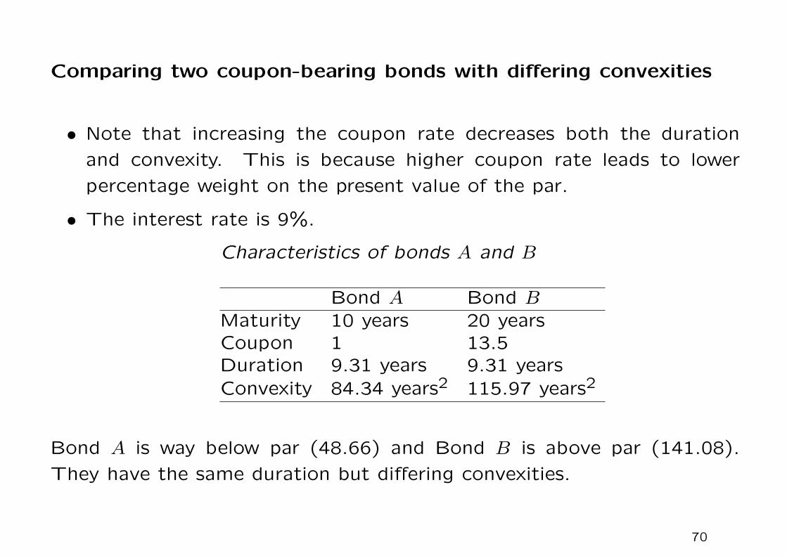
Comparing two coupon-bearing bonds with differing convexities

• Note that increasing the coupon rate decreases both the duration

and convexity. This is because higher coupon rate leads to lower

percentage weight on the present value of the par.

• The interest rate is 9%.

Characteristics of bonds A and B

Bond A Bond BMaturity 10 years 20 yearsCoupon 1 13.5Duration 9.31 years 9.31 yearsConvexity 84.34 years2 115.97 years2

Bond A is way below par (48.66) and Bond B is above par (141.08).

They have the same duration but differing convexities.

70

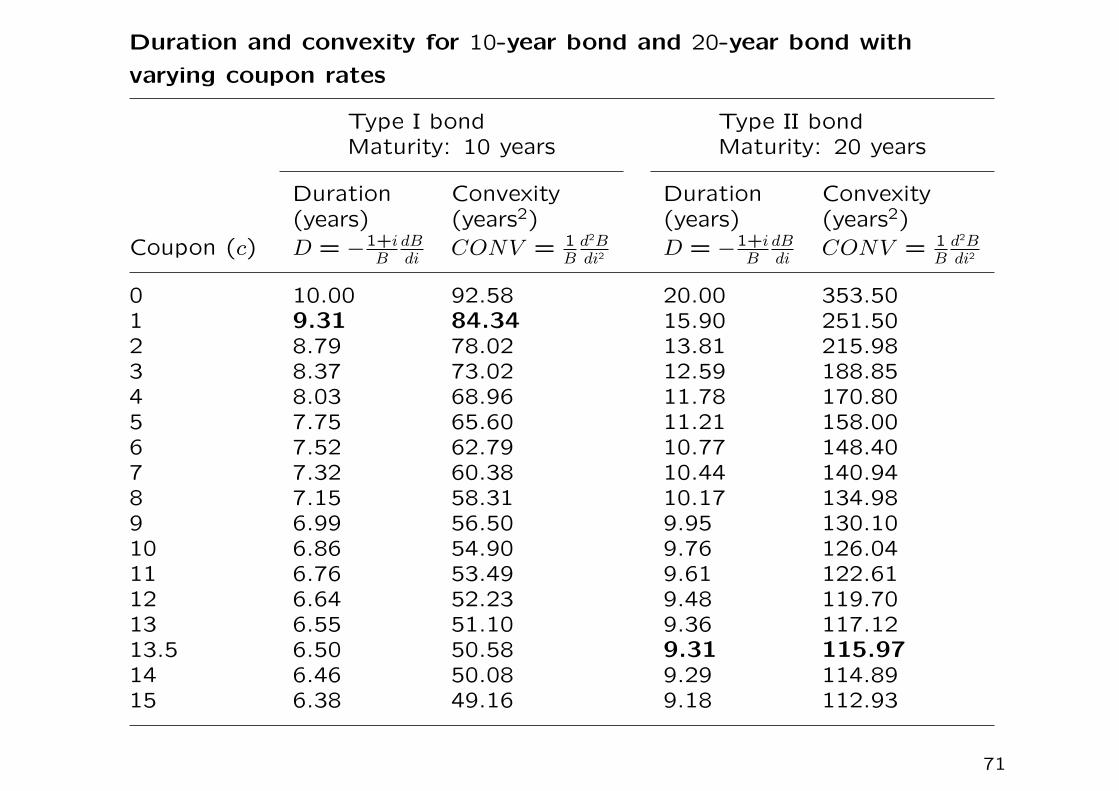
Duration and convexity for 10-year bond and 20-year bond with

varying coupon rates

Type I bond Type II bondMaturity: 10 years Maturity: 20 years

Duration Convexity Duration Convexity(years) (years2) (years) (years2)

Coupon (c) D = −1+iB

dBdi

CONV = 1B

d2Bdi2

D = −1+iB

dBdi

CONV = 1B

d2Bdi2

0 10.00 92.58 20.00 353.501 9.31 84.34 15.90 251.502 8.79 78.02 13.81 215.983 8.37 73.02 12.59 188.854 8.03 68.96 11.78 170.805 7.75 65.60 11.21 158.006 7.52 62.79 10.77 148.407 7.32 60.38 10.44 140.948 7.15 58.31 10.17 134.989 6.99 56.50 9.95 130.1010 6.86 54.90 9.76 126.0411 6.76 53.49 9.61 122.6112 6.64 52.23 9.48 119.7013 6.55 51.10 9.36 117.1213.5 6.50 50.58 9.31 115.9714 6.46 50.08 9.29 114.8915 6.38 49.16 9.18 112.93

71

The 20-year bond (B) can be made to have the same duration as that

of the 10-year bond (A) by setting a very high coupon rate. Bond B still

has a higher convexity.

Case 1: H = D

Set the horizon H to be the common duration of 9.31 years.

The horizon rates of return for bonds A and B move up even i increases

or decreases from i0 = 9% (see the tables on the next page). Comparing

the future value at H = 9.31 for the same initial value of $1,000,000, a

difference of $14,023 is resulted under different convexities.

72

• Suppose that the initial rates are 9% and that they quickly move up

by 1 or 2% or drop by the same amount. The horizon rate of return

in excess of 9% for the more convex bond is tenfold that of the bond

with lower convexity.

Horizon rates of return for A and B with H = 9.31 years when the ratesmove quickly from 9% to another value and stay there

Scenario

i = 7% i = 8% i = 9% i = 10% i = 11%

Bond A 9.008% 9.002% 9% 9.002% 9.008%

Bond B 9.085% 9.021% 9% 9.020% 9.079%

Suppose the same current value of 1 million and interest rate decreases

from 9% to 7%. We observe

• investment in A: 1,000,000(1 + 0.9008)9.31 = 2,232,222

• investment in B: 1,000,000(1 + 0.9085)9.31 = 2,246,245

This implies a difference of $2,246,245 − $2,232,222 = $14,023 in

the future value for no trouble at all, except looking up the value of

convexity.

73

Case 2: H < D

• Two short horizons have been chosen in the two bonds: H = 1 and

H = 2.

The gain in bond value when the interest rate decreases is more

substantial for the bond with higher convexity.

• Shorter horizon, the gain of horizon rate of return of Bond B is more

significant.

• At H = 1, with an increase in interest rate from 9% to 11%, the

convexity of B will cushion the loss from 6.2% to 5.7%.

74

Horizon rates of return when i takes a new value immediately after thepurchase of bond A and bond B (in annualized percentage)

Horizon (in years)and rates of returnfor A and B

Scenario

i = 7% i = 8% i = 9% i = 10% i = 11%

H = 1

RA 27.2 17.1 9.0 1.0 -6.2

RB 28.1 17.9 9.0 1.2 -5.7

H = 2

RA 16.7 12.7 9.0 5.4 2.0

RB 17.1 12.8 9.0 5.5 2.3

75

Duration and Convexity for a zero-coupon bond

Bond A(zero-coupon) Bond B

Coupon 0 9

Maturity 10.58 years 25 years

Duration 10.58 years 10.58 years

Convexity 103.12 years2 159.17 years2

Rates of return of A and B when i moves from i = 9% to another value after the bondhas been bought (horizon is set equal the duration)

Scenario

i = 7% i = 8% i = 9% i = 10% i = 11%

Bond A (zero-coupon) 9 9 9 9 9

Bond B 9.14 9.04 9 9.02 9.08

76

Recall C = S+D(D+1)(1+i)2

. Though S = 0 for a zero coupon bond, its

convexity remains positive since C = D(D+1)(1+i)2

when S = 0.

For the zero-coupon bond, when the horizon H is set to be the bond’s

maturity date T (so H = D = T ), the future value FH remains to be equal

to par under an increase or decrease of the interest rate since there is no

coupon within the time horizon. We then have FH = par = B0(1+ rH)H,

so rH does not change.

77

Looking for convexity in building a bond portfolio

Suppose we are unable to find a bond with the same duration and higher

convexity as the one we are considering buying. We may build a barbell

portfolio that have the same duration but higher convexity.

Price duration (years) Convexity (years)

Bond 1 $105.96 5 28.62Bond 2 $102.80 1 1.75Bond 3 $97.91 9 95.72

Portfolio $105.96 5 48.73

Portfolio consists of N2 = 0.5153 units of Bond 2 and N3 = 0.5411 units

of Bond 3. The weights N2 and N3 are obtained by equating the bond

value and duration, which give

N2B2 +N3B3 = B1 andN2B2

B1D2 +

N3B3

B1D3 = D1.

The barbell portfolio is seen to have higher convexity (48.73 for the port-

folio versus 28.62 for Bond 1). However, it is likely that the portfolio has

lower yield than that of Bond 1 due to convexity of the yield curve.

78

1. Comparison of bond values under changes in interest rate

Values of bond 1 and the barbell portfolio P for various

values of interest rate

i B1(i) BP (i)

4% 122.28 123.485% 116.50 116.996% 111.06 111.187% 105.96 105.968% 101.16 101.259% 96.64 97.00

10% 92.38 93.15

BP (i) always achieves higher value than B1(i) under varying values of

i.

The numerical results on the bond values are consistent with the plots

of bond values shown on P.59.

79

2. Comparison of horizon rate of return under changes in interest rate

5-year horizon rates of return for bond 1 and the barbell

portfolio

i r1H=5 rPH=54% 7.023% 7.230%5% 7.010% 7.100%6% 7.003% 7.025%7% 7% 7%8% 7.003% 7.024%9% 7.010% 7.092%

10% 7.023% 7.203%

r1H=5 < rPH=5 for all varying values of i.

80

Asset and liabilities management

• How should a pension fund, or an insurance company, set up its asset

portfolio in such a way as to be practically certain that it will be able

to meet its payment obligations in the future?

Redington conditions

Assume that the liabilities flow Lt, t = 1, . . . , T and assets flow At, t =

1, . . . , T , are known.

Interest rate term structure is flat, equal to i. The present value of the

liabilities and assets are

L =T∑

t=1

Lt

(1 + i)tand A =

T∑t=1

At

(1 + i)t.

We assume that the net value N = A− L = 0 initially.

81

How should one choose the structure of the assets such that this net

value does not change in the event of a change in interest rate?

First order condition (first Redington condition):

N = A− L to be insensitive to i.

SetdN

di=

1

1+ i

T∑t=1

t(Lt −At)(1 + i)−t =1

1+ i(DLL−DAA)

=A

1+ i(DL −DA) = 0, (since L = A),

where

DL =T∑

t=1

tLt

L

1

(1 + i)tand DA =

T∑t=1

tAt

L

1

(1 + i)t.

To satisfy the first Redington condition, we need to observe equality of

the two durations, DL and DA.

82

Recall that

∆N = ∆(A− L) ≈(d2A

di2−

d2L

di2

)∆i2

when A and L have the same duration.

In order that N remains positive, a sufficient condition is given by N(i)

being a convex function of i within that interval. This is captured by

Second Redington condition:d2A

di2>

d2L

di2.

Once the duration is set to be the same for both A and L, convexity

depends positively on the dispersion S of the cash flows. Therefore, a

sufficient condition for the second Redington condition is that the disper-

sion of the inflows from the assets is larger than that of the outflows to

the liabilities.

83

Example (Savings and Loan Associations in US in early 1980s)

They had deposits with short maturities (duration) while their loans to

mortgage developers had very long durations, since they financed mainly

housing projects. Their assets are loans to housing projects while their

liabilities are deposits.

• When the interest rates climbed sharply, the net worth of the Savings

and Loans Associations fall drastically.

In this case, even the first Redington condition was not met. This

spelled disaster.

84

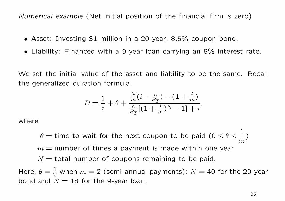
Numerical example (Net initial position of the financial firm is zero)

• Asset: Investing $1 million in a 20-year, 8.5% coupon bond.

• Liability: Financed with a 9-year loan carrying an 8% interest rate.

We set the initial value of the asset and liability to be the same. Recall

the generalized duration formula:

D =1

i+ θ +

Nm(i− c

BT)− (1 + i

m)

cBT

[(1 + im)N − 1] + i

,

where

θ = time to wait for the next coupon to be paid (0 ≤ θ ≤1

m)

m = number of times a payment is made within one year

N = total number of coupons remaining to be paid.

Here, θ = 12 when m = 2 (semi-annual payments); N = 40 for the 20-year

bond and N = 18 for the 9-year loan.

85

We obtain the respective duration of the asset and liability as

DA = 9.944 years and DL = 6.583 years.

To secure profits in operating loans and savings, the housing loans inter-

est rate should be higher than the deposits interest rates. Therefore, we

must have iA > iL. For iA = 8.5% and iL = 8%, the modified durations

are

DmA =DA

1+ iA= 9.165 years and DmL =

DL

1+ iL= 6.095 years.

Note that

∆VAVA

≈dVAVA

= −DmA diA and∆VLVL

≈dVLVL

= −DmL diL

86

so that

∆VP = ∆VA −∆VL ≈ −(DmAVA diA −DmLVL diL).

Suppose iA and iL receive the same increment and VA = VL, we have

∆VP ≈ −(DmA −DmL)VA di = −3.070VA di.

Based on the linear approximation, if the interest rate increases by 1%,

the net value of the project diminishes by 3.070% of the asset. Its risk

exposure presents a net modified duration of DmA −DmL = 3.070.

87

Summary

1. Immunization is a short-term series of measures destined to match

sensitivities of assets and liabilities. As time passes, these sensitivities

continue to change since the duration does not generally decrease in

the same amount as the planning horizon with the passage of time.

2. Whenever interest rates change, the duration also changes. Financial

manager may also want to pay special attention to the convexity of

his assets and liabilities as well.

3. So far we have considered flat term structures and parallel displace-

ments of them. More refined duration measures and analysis are

required if we do not face such flat structures. The next level of

more refined analysis is the use of deterministic term structure of

spot rates.

88

Measuring the riskiness of foreign currency-denominated bonds

Let B be the value of a foreign bond in foreign currency, e be the exchange

rate (value of one unit of foreign currency in domestic currency), V be

the value of the foreign bond in domestic currency. We have

V = eB

so thatdV

V=

dB

B+

de

e.

All the three relative changes are random variables. Observe that

dB

B=

1

B

dB

didi = −

D

1+ idi

so thatdV

V= −

D

1+ idi+

de

e.

Recall that

var(X + Y ) = var(X) + var(Y ) + 2cov(X,Y ).

89

We then deduce that

var(dV

V

)=(

D

1+ i

)2var(di) + var(

de

e)− 2

D

1+ icov(di,

de

e).

• The covariance between changes in interest rates and modifications

in the exchange rates is usually very low. The bulk of the variance of

changes in the foreign bond’s value stems mainly from the variance

of the exchange rate.

• Empirical studies show that the share of the exchange rate variance

is easily two-thirds of the total variance.

For finite changes in e and B, the correct formula should be

∆V

V=

(B +∆B)(e+∆e)−Be

Be=

∆B

B+

∆e

e+

∆B

B

∆e

e.

The second order term can be significant when∆B

Band

∆e

eare large.

90

Numerical example

Suppose that the loss on the Jakarta stock market was 60% in a given

period and that the rupee lost 60% of its value against the dollar in the

same period.

• The rate of change in the investment’s value in American dollars

cannot be (−60%)+(−60%) = (−120%). It does not make sense to

have a loss of more than 100%.

• It is more proper to use

∆V

V= (−60%)+ (−60%)+ (−60%)(−60%)

= −120%+ 36% = −84%.

91

Cash matching problem – Linear programming with constraints

• A known sequence of future monetary obligations over n periods:

y = (y1 . . . yn).

• Purchase bonds of various maturities and use the coupon payments

and redemption values to meet the obligations.

Suppose there are m bonds, and the cash stream on dates 1,2, . . . , n

associated with one unit of bond j is cj = (c1j . . . cnj), j = 1,2, . . . ,m.

pj = price of bond j

xj = amount of bond j held in the portfolio

Minimizem∑

j=1

pjxj

subject tom∑

j=1

cijxj ≥ yi i = 1,2, · · · , n

xj ≥ 0 j = 1,2, · · · ,m.

92

Numerical example – Six-year match of cash obligations using 10

bonds

Cash matching example

Bonds

Yr 1 2 3 4 5 6 7 8 9 10 Req’d Actual

1 10 7 8 6 7 5 10 8 7 100 100 171.74

2 10 7 8 6 7 5 10 8 107 200 200.00

3 10 7 8 6 7 5 110 108 800 800.00

4 10 7 8 6 7 105 100 119.34

5 10 7 8 106 107 800 800.00

6 110 107 108 1,200 1,200.00

p 109 94.8 99.5 93.1 97.2 92.9 110 104 102 95.2 2,381.14

x 0 11.2 0 6.81 0 0 0 6.3 0.28 0 Cost

In two of the 6 years (Year One and Year Four), some extra cash is

generated beyond what is required. Note that in Year Four, we have

11.2× 7+ 6.81× 6 = 119.34 > 100.

93

Difficulties and weaknesses

• There are high liabilities outflows in some years so a larger number of

bonds must be purchased that mature on those dates. These bonds

generate coupon payments in earlier years and only a portion of these

payments is needed to meet obligations in these early years. Such

problem is alleviated with a smoother set of liabilities outflows.

• At the end of Year 6, the cash flow required is $1,200, so either Bond

1, Bond 2 and / or Bond 3 must be purchased. Bond 2 is chosen

since it has lower coupon payments in earlier years so that less extra

cash is generated in those earlier years.

• Liabilities are being met by coupon payments or principals of maturing

bonds. Under passive static bond portfolio management, there will be

no sale or acquisition of bonds. The only risk is default risk. Adverse

interest rate changes do not affect the ability to meet liabilities.

94

• For typical liabilities schedule and bonds available for cash flow match-

ing, perfect matching is unlikely.

• We strike the tradeoff between (i) avoidance of the risk of not satis-

fying the liabilities stream (ii) lower cost in building the bond portfolio

that meets the liabilities.

• How to combine immunization with cash matching? More precisely,

how one strikes the balance between lower cost of constructing the

bond portfolio against smaller difference in duration (more ideal to

have higher convexity as well).

• The extra surpluses should be reinvested so this creates reinvestment

risks. This requires the estimation of the future interest rate move-

ments as well.

95

1.4 Optimal management and dynamic programming

Dynamic programming solves a problem step by step, starting at the

terminal time and working back to the beginning. This is commonly

called the“backward induction procedure”. From the end of a problem

or situation, we determine a sequence of optimal actions. It proceeds

by first considering the last time an optimal decision might be made and

choosing what to do in any situation at that time. Using this information,

one can then determine what to do at the second-to-last time of decision.

We use the one-period discount factor dk and evaluate the present value

step by step. In running dynamic programming, we assign to each node a

value equal to the best running present value that can be obtained from

that node.

For the ith node at time k, denoted by (k, i), the best running value is

called Vki. We refer to these values as V -values.

96

The V -values at the final nodes are just the terminal values of the invest-

ment process. Usually, the V -values at the final nodes are known as part

of the problem description.

Recurrence relation

Define caki to be the cash flow generated by moving from node (k, i) to

node (k +1, a). The recursion procedure is

Vki = maximizea

(caki + dkVk+1,a).

97

First recursive step of dynamic programming. For any node at time

n− 1, we find the maximum running present value from that node.

98

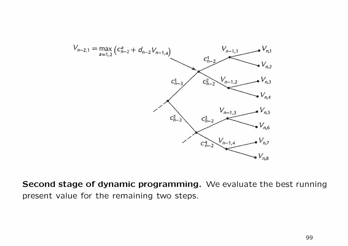
Second stage of dynamic programming. We evaluate the best running

present value for the remaining two steps.

99

Example – Fishing problem

• If you do not fish, the fish population doubles in the next year.

• If you fish and extract 70% of the fish, then the fish population will

grow to the same amount at the beginning of next fishing season.

The interest rate is constant at 25%, which means that the discount

factor is 0.8 per year. The initial fish population is 10 tons. The profit is

$1 per ton.

Remark

In this example, we fix the percentage of fish extracted to be 70%. In

the next example, we relax this constraint of fixing the percentage of

extraction.

100

The node values are the tonnage of fish in the lake; the branch values

are cash flows.

101

The node values are now the optimal running present values, found by

working backward from the terminal nodes. The branch values are cash

flows.

102

Once we are in Year Three, we can no longer fish. Therefore, we assign

the value of 0 to each of the final nodes. By backward induction, at each

of the nodes one step from the end, we determine the maximum possible

cash flow.

This determines the cash flow received in that season, and we assume

that we obtain that cash of selling the fish at the beginning of the season.

Hence we do not discount the profit. The value obtained is the (running)

present value, as viewed from that time.

Next we back up one time period and calculate the maximum present

values at that time. For example, for the node just to the right of the

initial node, we have

V = max(0.8× 28,14+ 0.8× 14).

The maximum is attained by the second choice, corresponding to the

downward branch, and hence V = 14 + 0.8 × 14 = 25.2. The discount

rate of 1/1.25 = 0.8 is applicable at every stage.

103

For the node below, we compute

V = max(0.8× 14,7+ 0.8× 7) = 12.6.

For the initial node, we obtain

V = max(0.8× 25.2,7+ 0.8× 12.6) = 20.16.

The value at the initial node gives the maximum present value. The

optimal path is the path determined by the optimal choices we discovered

in the procedure.

The optimal path is indicated by the heavy line. In words, the solution is

not to fish the first season (to let the fish population increase) and then

fish the next two seasons (to harvest the population).

104

Example – Mining

The mine has been worked heavily and is approaching depletion. If x is

the amount of gold remaining in the mine at the beginning of a year, the

cost to extract z < x ounces of gold in that year is $500z2/x. Note that

as x decreases, it becomes more difficult to obtain gold. This particular

form of the cost as a square function of z allows simple solution in the

backward induction procedure.

It is estimated that the current amount of gold remaining in the mine is

x0 = 50,000 ounces. The price of gold is $400/oz.

We are considering the purchase of a 10-year lease of the mine. The

interest rate is 10%. How much is this lease worth?

Note that the extraction amount z in each year is the control variable

whose value is to be determined in the dynamic programming procedure

at each time step.

105

Backward induction procedure

We begin by determining the value of a lease on the mine at time 9,

when the remaining deposit is x9. Only 1 year remains on the lease, so

the value is obtained by maximizing the profit for that year. If we extract

z9 ounces, the revenue from the sale of the gold will be gz9, where g is

the price of gold, and the cost of mining will be 500z29/x9. Hence the

optimal value of the mine at time 9 if x9 is the remaining deposit level is

V9(x9) = maxz9

(gz9 − 500z29/x9).

We find the maximum by setting the derivative with respect to z9 equal

to zero. This yields

z9 = gx9/1,000.

We should check that z9 ≤ x9, which does hold with the values we use.

106

We substitute this value in the formula for profit to find

V9(x9) =g2x91,000

−500g2x9

1,000× 1,000=

g2x92,000

.

We write this as V9(x9) = K9x9, where K9 = g2/2,000 is a constant.

Hence the value of the lease is directly proportional to how much gold

remains in the mine; the proportionality factor is K9.

Next we back up and solve for V8(x8). In this case we account for the

profit generated during the ninth year and also for the value that the lease

will have at the end of that year – a value that depends on how much

gold we leave in the mine. Hence,

V8(x8) = maxz8

[gz8 − 500z28/x8 + dV9(x8 − z8)].

Note that we have discounted the value associated with the mine at the

next year by a factor d. As in the previous example, the discount rate is

constant because the spot rate curve is flat. In this case, d = 1/1.1.

107

Using the explicit form for the function V9, we may write

V8(x8) = maxz8

[gz8 − 500z28/x8 + dK9(x8 − z8)].

We again set the derivative with respect to z8 equal to zero and obtain

z8 =(g − dK9)x8

1,000.

This value can be substituted into the expression for V8 to obtain

V8(x8) =

[(g − dK9)

2

2,000+ dK9

]x8.

This is proportional to x8, and we may write it as V8(x8) = K8x8.

We can continue backward in this way, determining the functions V7, V6, . . . ,

V0. Each of these functions will be of the form Vj(xj) = Kjxj. It is seen

that the same algebra applies at each step, and hence we have the recur-

sive formula

Kj =(g − dKj+1)

2

2,000+ dKj+1.

108

If we use the specific values g = 400 and d = 1/1.1, we begin the backward

recursion with K9 = g2/2,000 = 80. We can then easily solve for all the

other values, as shown in the Table, working from the right to the left.

Year 0 1 2 3 4 5 6 7 8 9

K-value 213.81 211.45 208.17 203.58 197.13 187.96 174.79 155.47 126.28 80.00

K-values for the mine

It is K0 that determines the value of the original lease, which is determined

by finding the value of the lease when there is 50,000 ounces of gold

remaining. Hence V0(50,000) = 213.82× 50,000 = $10,691,000.

109

The optimal plan is determined as a by-product of the dynamic program-

ming procedure. At any time j, the amount of gold to extract is the

value zj found in the optimization problem. Hence z9 = gx9/1,000 and

z8 = (g − dK9)x8/1,000. In general, we obtain

zj = (g − dKj+1)xj/1,000.

We start from x0 = 50,000, then

z0 =8− dK1

1,00050,000 =

400− 211.451.1

1,00050,000 = 10,388.6.

Next, x1 = x0 − z0 = 39,611.4. We then have

z1 =400− 208.17

1.1

1,00039,611.4 = 7,716.

In Qn 10 of HW 1, we consider the perpetual ownership of the mine. In

this case, the K-values are independent of the years of operation. The

corresponding equation for the common K is given by

K =(g − dK)2

2000+ dK.

110