math 590: meshfree methods - applied mathematicsfass/590/notes/notes590_ch12.pdf · math 590:...
TRANSCRIPT

MATH 590: Meshfree MethodsStable Computation via the Hilbert–Schmidt SVD
Greg Fasshauer
Department of Applied MathematicsIllinois Institute of Technology
Fall 2014
[email protected] MATH 590 1

Outline
1 Introduction
2 Contour-Padé – The First Stable Algorithm
3 The Hilbert–Schmidt SVD
4 Implementation Issues in Higher Dimensions
[email protected] MATH 590 2

Introduction
Outline
1 Introduction
2 Contour-Padé – The First Stable Algorithm
3 The Hilbert–Schmidt SVD
4 Implementation Issues in Higher Dimensions
[email protected] MATH 590 3

Introduction
As we’ve mentioned several times before, there are a number offeatures that make positive definite kernels (or RBFs) so attractive towork with:
Interpolants with “flat” kernels converge to polynomial interpolants.
Gaussians (and certain other RBFs) providedimension-independent, arbitrarily high, convergence rates forsufficiently “nice” data (i.e., with low effective dimension andcoming from a smooth function).
Numerical instability of interpolation/approximation algorithms canbe overcome by using a “better” basis.
All of this together establishes (smooth) RBFs as generalizedspectral methods.
[email protected] MATH 590 4

Introduction
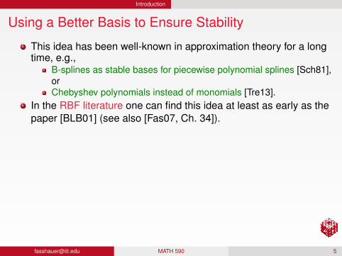
Using a Better Basis to Ensure Stability
This idea has been well-known in approximation theory for a longtime, e.g.,
B-splines as stable bases for piecewise polynomial splines [Sch81],orChebyshev polynomials instead of monomials [Tre13].
In the RBF literature one can find this idea at least as early as thepaper [BLB01] (see also [Fas07, Ch. 34]).The use of expansions in terms of eigenvalues and eigenfunctionsof the Hilbert–Schmidt integral operator K associated with thekernel K to obtain stable bases for kernel spaces HK (X ) isdiscussed in [CFM14, Fas11a, Fas11b, FM12], and implicitlyappeared in [FP08].
Gaussian eigenvalues and eigenfunctions were presented in theprevious chapter.iterated Brownian bridge kernels were discussed in Chapter 6.
We now explain how to use such expansions to obtain theHilbert–Schmidt SVD.
[email protected] MATH 590 5
Introduction
Using a Better Basis to Ensure Stability
This idea has been well-known in approximation theory for a longtime, e.g.,
B-splines as stable bases for piecewise polynomial splines [Sch81],orChebyshev polynomials instead of monomials [Tre13].
In the RBF literature one can find this idea at least as early as thepaper [BLB01] (see also [Fas07, Ch. 34]).
The use of expansions in terms of eigenvalues and eigenfunctionsof the Hilbert–Schmidt integral operator K associated with thekernel K to obtain stable bases for kernel spaces HK (X ) isdiscussed in [CFM14, Fas11a, Fas11b, FM12], and implicitlyappeared in [FP08].
Gaussian eigenvalues and eigenfunctions were presented in theprevious chapter.iterated Brownian bridge kernels were discussed in Chapter 6.
We now explain how to use such expansions to obtain theHilbert–Schmidt SVD.
[email protected] MATH 590 5

Introduction
Using a Better Basis to Ensure Stability
This idea has been well-known in approximation theory for a longtime, e.g.,
B-splines as stable bases for piecewise polynomial splines [Sch81],orChebyshev polynomials instead of monomials [Tre13].
In the RBF literature one can find this idea at least as early as thepaper [BLB01] (see also [Fas07, Ch. 34]).The use of expansions in terms of eigenvalues and eigenfunctionsof the Hilbert–Schmidt integral operator K associated with thekernel K to obtain stable bases for kernel spaces HK (X ) isdiscussed in [CFM14, Fas11a, Fas11b, FM12], and implicitlyappeared in [FP08].
Gaussian eigenvalues and eigenfunctions were presented in theprevious chapter.iterated Brownian bridge kernels were discussed in Chapter 6.
We now explain how to use such expansions to obtain theHilbert–Schmidt SVD.
[email protected] MATH 590 5
Contour-Padé – The First Stable Algorithm
Outline
1 Introduction
2 Contour-Padé – The First Stable Algorithm
3 The Hilbert–Schmidt SVD
4 Implementation Issues in Higher Dimensions
[email protected] MATH 590 6

Contour-Padé – The First Stable Algorithm
The Contour-Padé algorithm was the subject of Grady Wright’s Ph.D.thesis [Wri03] and was reported in [FW04] (see also [Fas07, Ch. 17]).
The aim of the Contour-Padé algorithm is to come up with a methodthat allows the computation and evaluation of RBF interpolants forinfinitely smooth basic functions when the shape parameter ε tends tozero (including the limiting case).
The starting point is to consider evaluation of the RBF interpolant
sε(x) =N∑
j=1
cjκ(ε‖x − x j‖)
for a fixed evaluation point x as an analytic function of ε.
[email protected] MATH 590 7
Contour-Padé – The First Stable Algorithm
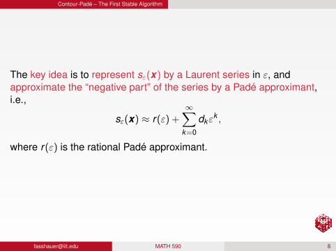
The key idea is to represent sε(x) by a Laurent series in ε, andapproximate the “negative part” of the series by a Padé approximant,i.e.,
sε(x) ≈ r(ε) +∞∑
k=0
dkεk ,
where r(ε) is the rational Padé approximant.
[email protected] MATH 590 8

Contour-Padé – The First Stable Algorithm
We then rewrite the interpolant in cardinal form, i.e., as
sε(x) =N∑
j=1
cjκ(ε‖x − x j‖)
= k ε(x)T c= k ε(x)T K−1
ε y
=(?uε(x)
)Ty ,
where k ε(x)j = κ(ε‖x − x j‖), (Kε)i,j = κ(ε‖x i − x j‖),c = (c1, . . . , cN)T , y = (y1, . . . , yN)T , and
?uε(x) = K−1
ε k ε(x)
denotes the vector of values of the cardinal functions at x .
[email protected] MATH 590 9

Contour-Padé – The First Stable Algorithm
We then rewrite the interpolant in cardinal form, i.e., as
sε(x) =N∑
j=1
cjκ(ε‖x − x j‖)
= k ε(x)T c
= k ε(x)T K−1ε y
=(?uε(x)
)Ty ,
where k ε(x)j = κ(ε‖x − x j‖), (Kε)i,j = κ(ε‖x i − x j‖),c = (c1, . . . , cN)T , y = (y1, . . . , yN)T , and
?uε(x) = K−1
ε k ε(x)
denotes the vector of values of the cardinal functions at x .
[email protected] MATH 590 9

Contour-Padé – The First Stable Algorithm
We then rewrite the interpolant in cardinal form, i.e., as
sε(x) =N∑
j=1
cjκ(ε‖x − x j‖)
= k ε(x)T c= k ε(x)T K−1
ε y
=(?uε(x)
)Ty ,
where k ε(x)j = κ(ε‖x − x j‖), (Kε)i,j = κ(ε‖x i − x j‖),c = (c1, . . . , cN)T , y = (y1, . . . , yN)T , and
?uε(x) = K−1
ε k ε(x)
denotes the vector of values of the cardinal functions at x .
[email protected] MATH 590 9

Contour-Padé – The First Stable Algorithm
We then rewrite the interpolant in cardinal form, i.e., as
sε(x) =N∑
j=1
cjκ(ε‖x − x j‖)
= k ε(x)T c= k ε(x)T K−1
ε y
=(?uε(x)
)Ty ,
where k ε(x)j = κ(ε‖x − x j‖), (Kε)i,j = κ(ε‖x i − x j‖),c = (c1, . . . , cN)T , y = (y1, . . . , yN)T , and
?uε(x) = K−1
ε k ε(x)
denotes the vector of values of the cardinal functions at x .
[email protected] MATH 590 9

Contour-Padé – The First Stable Algorithm
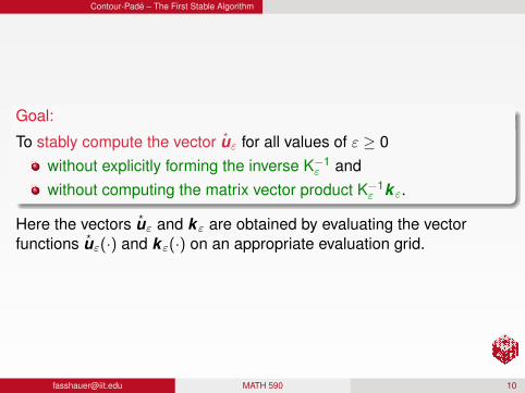
Goal:
To stably compute the vector?uε for all values of ε ≥ 0
without explicitly forming the inverse K−1ε and
without computing the matrix vector product K−1ε k ε.
Here the vectors?uε and k ε are obtained by evaluating the vector
functions?uε(·) and k ε(·) on an appropriate evaluation grid.
[email protected] MATH 590 10

Contour-Padé – The First Stable Algorithm
Goal:
To stably compute the vector?uε for all values of ε ≥ 0
without explicitly forming the inverse K−1ε and
without computing the matrix vector product K−1ε k ε.
Here the vectors?uε and k ε are obtained by evaluating the vector
functions?uε(·) and k ε(·) on an appropriate evaluation grid.
[email protected] MATH 590 10

Contour-Padé – The First Stable Algorithm
The solution proposed by Wright and Fornberg is to use Cauchy’sintegral theorem to integrate around a circle in the complexε-plane.
The residuals (i.e., coefficients in the Laurent expansion) areobtained using the (inverse) fast Fourier transform.The terms with negative powers of ε are then approximated usinga rational Padé approximant.The integration contour (usually a circle) has to lie between theregion of instability near ε = 0 and possible branch pointsingularities that lie somewhere in the complex plane dependingon the choice of κ.Details of the method can be found in [FW04].
[email protected] MATH 590 11
Contour-Padé – The First Stable Algorithm
The solution proposed by Wright and Fornberg is to use Cauchy’sintegral theorem to integrate around a circle in the complexε-plane.The residuals (i.e., coefficients in the Laurent expansion) areobtained using the (inverse) fast Fourier transform.
The terms with negative powers of ε are then approximated usinga rational Padé approximant.The integration contour (usually a circle) has to lie between theregion of instability near ε = 0 and possible branch pointsingularities that lie somewhere in the complex plane dependingon the choice of κ.Details of the method can be found in [FW04].
[email protected] MATH 590 11
Contour-Padé – The First Stable Algorithm
The solution proposed by Wright and Fornberg is to use Cauchy’sintegral theorem to integrate around a circle in the complexε-plane.The residuals (i.e., coefficients in the Laurent expansion) areobtained using the (inverse) fast Fourier transform.The terms with negative powers of ε are then approximated usinga rational Padé approximant.
The integration contour (usually a circle) has to lie between theregion of instability near ε = 0 and possible branch pointsingularities that lie somewhere in the complex plane dependingon the choice of κ.Details of the method can be found in [FW04].
[email protected] MATH 590 11

Contour-Padé – The First Stable Algorithm
The solution proposed by Wright and Fornberg is to use Cauchy’sintegral theorem to integrate around a circle in the complexε-plane.The residuals (i.e., coefficients in the Laurent expansion) areobtained using the (inverse) fast Fourier transform.The terms with negative powers of ε are then approximated usinga rational Padé approximant.The integration contour (usually a circle) has to lie between theregion of instability near ε = 0 and possible branch pointsingularities that lie somewhere in the complex plane dependingon the choice of κ.
Details of the method can be found in [FW04].
[email protected] MATH 590 11

Contour-Padé – The First Stable Algorithm
The solution proposed by Wright and Fornberg is to use Cauchy’sintegral theorem to integrate around a circle in the complexε-plane.The residuals (i.e., coefficients in the Laurent expansion) areobtained using the (inverse) fast Fourier transform.The terms with negative powers of ε are then approximated usinga rational Padé approximant.The integration contour (usually a circle) has to lie between theregion of instability near ε = 0 and possible branch pointsingularities that lie somewhere in the complex plane dependingon the choice of κ.Details of the method can be found in [FW04].
[email protected] MATH 590 11

Contour-Padé – The First Stable Algorithm
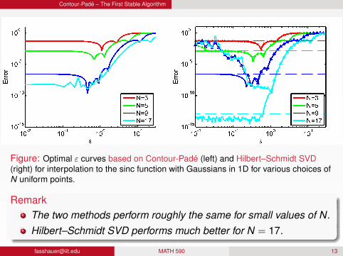
Figure: Optimal ε curves based on Contour-Padé (left) and Hilbert–Schmidt SVD(right) for interpolation to the sinc function with Gaussians in 1D for various choices ofN uniform points.
RemarkThe two methods perform roughly the same for small values of N.Hilbert–Schmidt SVD performs much better for N = 17.
[email protected] MATH 590 13

Contour-Padé – The First Stable Algorithm
Figure: Optimal ε curves based on Contour-Padé (left) and Hilbert–Schmidt SVD(right) for interpolation to the 2D sinc function with Gaussians in for various choices ofN Halton points.
RemarkAgain, both methods perform equally well for small N, butHilbert–Schmidt SVD is much more accurate for N = 81.
[email protected] MATH 590 14

Contour-Padé – The First Stable Algorithm
RemarkThe main drawback of the Contour-Padé algorithm is the fact that if Nbecomes too large then the region of ill-conditioning around the originin the complex ε-plane and the branch point singularities will overlap.
This implies that the method can only be used with limited success.
Moreover, as the examples above show, the value of N that has to beconsidered “large” is unfortunately rather small. For theone-dimensional case the results for N = 17 already are affected byinstabilities, and in the two-dimensional experiment N = 81 causesproblems.
We now want to work our way toward the Hilbert–Schmidt SVD(Gauss-QR) method of [FM12].
[email protected] MATH 590 15

The Hilbert–Schmidt SVD
Outline
1 Introduction
2 Contour-Padé – The First Stable Algorithm
3 The Hilbert–Schmidt SVD
4 Implementation Issues in Higher Dimensions
[email protected] MATH 590 16

The Hilbert–Schmidt SVD General Framework
The following discussion is based mainly on [FM12], which developeda stable algorithm specifically for the Gaussian kernel.That algorithm was referred to as Gauss-QR algorithm, but it is aspecial case of the Hilbert–Schmidt SVD. Similar algorithms are alsoknown as RBF-QR algorithms.
The general framework applies to any kernel that has aHilbert–Schmidt (or Mercer) series
K (x , z) =∞∑
n=1
λnϕn(x)ϕn(z).
We now discuss the general framework and later look atkernel-specific issues that are important for the implementation.
[email protected] MATH 590 17

The Hilbert–Schmidt SVD General Framework
The first main idea is to use the eigenexpansion of the kernel K torewrite the matrix K from the interpolation problem as
K =
K (x1,x1) . . . K (x1,xN)...
...K (xN ,x1) . . . K (xN ,xN)
=
ϕ1(x1) . . . ϕM (x1) . . ....
...ϕ1(xN ) . . . ϕM (xN ) . . .
λ1
. . .λM
. . .
ϕ1(x1) . . . ϕ1(xN )
......
ϕM (x1) . . . ϕM (xN )...
...
Since
K (x i ,x j) =∞∑
n=1
λnϕn(x i)ϕn(x j) ≈M∑
n=1
λnϕn(x i)ϕn(x j)
accurate reconstruction of all entries of K will likely require M > N.We already looked at truncation lengths for iterated Brownian bridgekernels in Chapter 6 and HW 2.
[email protected] MATH 590 18
The Hilbert–Schmidt SVD General Framework
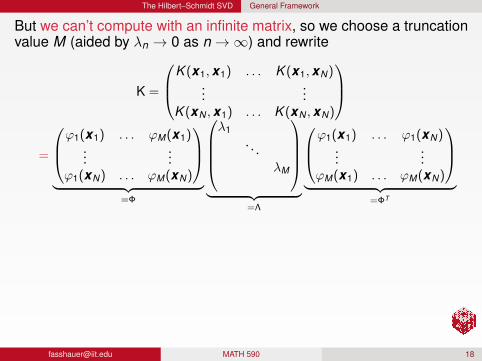
But we can’t compute with an infinite matrix, so we choose a truncationvalue M (aided by λn → 0 as n→∞) and rewrite
K =
K (x1,x1) . . . K (x1,xN)...
...K (xN ,x1) . . . K (xN ,xN)
=
ϕ1(x1) . . . ϕM(x1)...
...ϕ1(xN) . . . ϕM(xN)
︸ ︷︷ ︸
=Φ
λ1
. . .λM
︸ ︷︷ ︸
=Λ
ϕ1(x1) . . . ϕ1(xN)...
...ϕM(x1) . . . ϕM(xN)
︸ ︷︷ ︸
=ΦT
Since
K (x i ,x j) =∞∑
n=1
λnϕn(x i)ϕn(x j) ≈M∑
n=1
λnϕn(x i)ϕn(x j)
accurate reconstruction of all entries of K will likely require M > N.We already looked at truncation lengths for iterated Brownian bridgekernels in Chapter 6 and HW 2.
[email protected] MATH 590 18

The Hilbert–Schmidt SVD General Framework
RemarkA careful analysis of truncation lengths for general kernels given inseries form (which includes our truncated Mercer series kernels)is presented in [GRZ13].There it is shown that the truncation length M should needs todepend on N and the smallest eigenvalue of K. In fact, one shouldhave
∞∑n=M+1
λn .λmin(K)
N,
where . encodes a dependence on the size of the eigenfunctions.If M is chosen in this way then interpolation error with thetruncated kernel will be on the same order as with the full kernel.
This criterion has only limited practical applicability — especially ifwe have a very ill-conditioned matrix K and we want to use thetruncated kernel to obtain a stable basis.
[email protected] MATH 590 19

The Hilbert–Schmidt SVD General Framework
RemarkA careful analysis of truncation lengths for general kernels given inseries form (which includes our truncated Mercer series kernels)is presented in [GRZ13].There it is shown that the truncation length M should needs todepend on N and the smallest eigenvalue of K. In fact, one shouldhave
∞∑n=M+1
λn .λmin(K)
N,
where . encodes a dependence on the size of the eigenfunctions.If M is chosen in this way then interpolation error with thetruncated kernel will be on the same order as with the full kernel.This criterion has only limited practical applicability — especially ifwe have a very ill-conditioned matrix K and we want to use thetruncated kernel to obtain a stable basis.
[email protected] MATH 590 19

The Hilbert–Schmidt SVD General Framework
We now assume that M > N, so that Φ is “short and fat”.The key is to first partition the matrix Φ into two blocks Φ1 and Φ2according toϕ1(x1) . . . ϕN(x1) ϕN+1(x1) . . . ϕM(x1)
......
......
ϕ1(xN) . . . ϕN(xN) ϕN+1(xN) . . . ϕM(xN)
=
Φ1︸︷︷︸N×N
Φ2︸︷︷︸N×(M−N)
.
RemarkWe can think of the n-th column of Φ as a sample of the n-theigenfunction obtained at the interpolation locations x1, . . . ,xN .
Recall that the eigenfunctions are orthogonal in both L2(Ω, ρ) andin HK (Ω). However, this does not imply orthogonality of thecolumns of Φ.Thus, the Hilbert-Schmidt SVD does not employ orthogonalmatrices Φ1 (and later Ψ).
[email protected] MATH 590 20

The Hilbert–Schmidt SVD General Framework
We now assume that M > N, so that Φ is “short and fat”.The key is to first partition the matrix Φ into two blocks Φ1 and Φ2according toϕ1(x1) . . . ϕN(x1) ϕN+1(x1) . . . ϕM(x1)
......
......
ϕ1(xN) . . . ϕN(xN) ϕN+1(xN) . . . ϕM(xN)
=
Φ1︸︷︷︸N×N
Φ2︸︷︷︸N×(M−N)
.
RemarkWe can think of the n-th column of Φ as a sample of the n-theigenfunction obtained at the interpolation locations x1, . . . ,xN .Recall that the eigenfunctions are orthogonal in both L2(Ω, ρ) andin HK (Ω). However, this does not imply orthogonality of thecolumns of Φ.
Thus, the Hilbert-Schmidt SVD does not employ orthogonalmatrices Φ1 (and later Ψ).
[email protected] MATH 590 20

The Hilbert–Schmidt SVD General Framework
We now assume that M > N, so that Φ is “short and fat”.The key is to first partition the matrix Φ into two blocks Φ1 and Φ2according toϕ1(x1) . . . ϕN(x1) ϕN+1(x1) . . . ϕM(x1)
......
......
ϕ1(xN) . . . ϕN(xN) ϕN+1(xN) . . . ϕM(xN)
=
Φ1︸︷︷︸N×N
Φ2︸︷︷︸N×(M−N)
.
RemarkWe can think of the n-th column of Φ as a sample of the n-theigenfunction obtained at the interpolation locations x1, . . . ,xN .Recall that the eigenfunctions are orthogonal in both L2(Ω, ρ) andin HK (Ω). However, this does not imply orthogonality of thecolumns of Φ.Thus, the Hilbert-Schmidt SVD does not employ orthogonalmatrices Φ1 (and later Ψ).
[email protected] MATH 590 20

The Hilbert–Schmidt SVD General Framework
By replacing ΦT with its blocks and applying an analogous blockpartition to Λ we formally rewrite our eigen-decomposition of K:
K = ΦΛΦT
= Φ
(Λ1
Λ2
)(ΦT
1ΦT
2
)= Φ
(Λ1ΦT
1Λ2ΦT
2
)= Φ
(IN
Λ2ΦT2 Φ−T
1 Λ−11
)︸ ︷︷ ︸
=Ψ
Λ1ΦT1︸ ︷︷ ︸
=M
We have now identifieda preconditioning matrix M andmatrices
Ψ and Φ1 of left and right Hilbert-Schmidt singular vectors,respectively, andΛ1 of Hilbert-Schmidt singular values.
[email protected] MATH 590 21

The Hilbert–Schmidt SVD General Framework
By replacing ΦT with its blocks and applying an analogous blockpartition to Λ we formally rewrite our eigen-decomposition of K:
K = ΦΛΦT
= Φ
(Λ1
Λ2
)(ΦT
1ΦT
2
)
= Φ
(Λ1ΦT
1Λ2ΦT
2
)= Φ
(IN
Λ2ΦT2 Φ−T
1 Λ−11
)︸ ︷︷ ︸
=Ψ
Λ1ΦT1︸ ︷︷ ︸
=M
We have now identifieda preconditioning matrix M andmatrices
Ψ and Φ1 of left and right Hilbert-Schmidt singular vectors,respectively, andΛ1 of Hilbert-Schmidt singular values.
[email protected] MATH 590 21

The Hilbert–Schmidt SVD General Framework
By replacing ΦT with its blocks and applying an analogous blockpartition to Λ we formally rewrite our eigen-decomposition of K:
K = ΦΛΦT
= Φ
(Λ1
Λ2
)(ΦT
1ΦT
2
)= Φ
(Λ1ΦT
1Λ2ΦT
2
)
= Φ
(IN
Λ2ΦT2 Φ−T
1 Λ−11
)︸ ︷︷ ︸
=Ψ
Λ1ΦT1︸ ︷︷ ︸
=M
We have now identifieda preconditioning matrix M andmatrices
Ψ and Φ1 of left and right Hilbert-Schmidt singular vectors,respectively, andΛ1 of Hilbert-Schmidt singular values.
[email protected] MATH 590 21

The Hilbert–Schmidt SVD General Framework
By replacing ΦT with its blocks and applying an analogous blockpartition to Λ we formally rewrite our eigen-decomposition of K:
K = ΦΛΦT
= Φ
(Λ1
Λ2
)(ΦT
1ΦT
2
)= Φ
(Λ1ΦT
1Λ2ΦT
2
)= Φ
(IN
Λ2ΦT2 Φ−T
1 Λ−11
)︸ ︷︷ ︸
=Ψ
Λ1ΦT1︸ ︷︷ ︸
=M
We have now identifieda preconditioning matrix M andmatrices
Ψ and Φ1 of left and right Hilbert-Schmidt singular vectors,respectively, andΛ1 of Hilbert-Schmidt singular values.
[email protected] MATH 590 21

The Hilbert–Schmidt SVD General Framework
There are at least two ways to interpret the Hilbert–Schmidt SVD:
We have found an invertible M such that Ψ = KM−1 is betterconditioned than K (without forming K or computing with it).We have diagonalized the matrix K, i.e.,
K = ΨΛ1ΦT1
with diagonal matrix Λ1 of Hilbert-Schmidt singular values.Here, as above, equality is only up to machine accuracy (i.e., Mhas to be chosen large enough).
The matrix Ψ in the same for both interpretations, and it can becomputed stably.
Moreover, the notation above implies M = Λ1ΦT1 .
[email protected] MATH 590 22

The Hilbert–Schmidt SVD General Framework
There are at least two ways to interpret the Hilbert–Schmidt SVD:
We have found an invertible M such that Ψ = KM−1 is betterconditioned than K (without forming K or computing with it).
We have diagonalized the matrix K, i.e.,
K = ΨΛ1ΦT1
with diagonal matrix Λ1 of Hilbert-Schmidt singular values.Here, as above, equality is only up to machine accuracy (i.e., Mhas to be chosen large enough).
The matrix Ψ in the same for both interpretations, and it can becomputed stably.
Moreover, the notation above implies M = Λ1ΦT1 .
[email protected] MATH 590 22

The Hilbert–Schmidt SVD General Framework
There are at least two ways to interpret the Hilbert–Schmidt SVD:
We have found an invertible M such that Ψ = KM−1 is betterconditioned than K (without forming K or computing with it).We have diagonalized the matrix K, i.e.,
K = ΨΛ1ΦT1
with diagonal matrix Λ1 of Hilbert-Schmidt singular values.Here, as above, equality is only up to machine accuracy (i.e., Mhas to be chosen large enough).
The matrix Ψ in the same for both interpretations, and it can becomputed stably.
Moreover, the notation above implies M = Λ1ΦT1 .
[email protected] MATH 590 22

The Hilbert–Schmidt SVD General Framework
There are at least two ways to interpret the Hilbert–Schmidt SVD:
We have found an invertible M such that Ψ = KM−1 is betterconditioned than K (without forming K or computing with it).We have diagonalized the matrix K, i.e.,
K = ΨΛ1ΦT1
with diagonal matrix Λ1 of Hilbert-Schmidt singular values.Here, as above, equality is only up to machine accuracy (i.e., Mhas to be chosen large enough).
The matrix Ψ in the same for both interpretations, and it can becomputed stably.
Moreover, the notation above implies M = Λ1ΦT1 .
[email protected] MATH 590 22

The Hilbert–Schmidt SVD General Framework
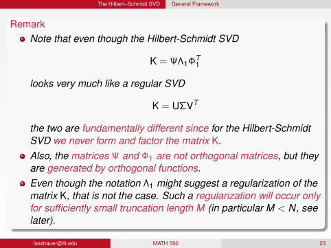
RemarkNote that even though the Hilbert-Schmidt SVD
K = ΨΛ1ΦT1
looks very much like a regular SVD
K = UΣVT
the two are fundamentally different since for the Hilbert-SchmidtSVD we never form and factor the matrix K.
Also, the matrices Ψ and Φ1 are not orthogonal matrices, but theyare generated by orthogonal functions.Even though the notation Λ1 might suggest a regularization of thematrix K, that is not the case. Such a regularization will occur onlyfor sufficiently small truncation length M (in particular M < N, seelater).
[email protected] MATH 590 23

The Hilbert–Schmidt SVD General Framework
RemarkNote that even though the Hilbert-Schmidt SVD
K = ΨΛ1ΦT1
looks very much like a regular SVD
K = UΣVT
the two are fundamentally different since for the Hilbert-SchmidtSVD we never form and factor the matrix K.Also, the matrices Ψ and Φ1 are not orthogonal matrices, but theyare generated by orthogonal functions.
Even though the notation Λ1 might suggest a regularization of thematrix K, that is not the case. Such a regularization will occur onlyfor sufficiently small truncation length M (in particular M < N, seelater).
[email protected] MATH 590 23
The Hilbert–Schmidt SVD General Framework
RemarkNote that even though the Hilbert-Schmidt SVD
K = ΨΛ1ΦT1
looks very much like a regular SVD
K = UΣVT
the two are fundamentally different since for the Hilbert-SchmidtSVD we never form and factor the matrix K.Also, the matrices Ψ and Φ1 are not orthogonal matrices, but theyare generated by orthogonal functions.Even though the notation Λ1 might suggest a regularization of thematrix K, that is not the case. Such a regularization will occur onlyfor sufficiently small truncation length M (in particular M < N, seelater).
[email protected] MATH 590 23

The Hilbert–Schmidt SVD General Framework
Taking a closer look at the matrix Ψ, we see that
Ψ = (Φ1 Φ2)
(IN
Λ2ΦT2 Φ−T
1 Λ−11
)= Φ1 + Φ2
[Λ2ΦT
2 Φ−T1 Λ−1
1
],
which we recognize asthe matrix Φ1 corresponding to samples of the first Neigenfunctionsplus an appropriate correction matrix.
[email protected] MATH 590 24

The Hilbert–Schmidt SVD General Framework
Viewed as functions, we have a new basis
ψ(·)T = (ψ1(·), . . . , ψN(·))
for the interpolation space
span K (·,x1), . . . ,K (·,xN)consisting of the appropriately corrected first N eigenfunctions:
RemarkThe data-dependence of the new basis is captured by the “correction”term (since Φ1 and Φ2 depend on the center locations). The new basisis more stable since we have removed Λ1.
[email protected] MATH 590 25

The Hilbert–Schmidt SVD General Framework
Viewed as functions, we have a new basis
ψ(·)T = (ψ1(·), . . . , ψN(·))
for the interpolation space
span K (·,x1), . . . ,K (·,xN)consisting of the appropriately corrected first N eigenfunctions:
k(x)T = φ(x)T(
INΛ2ΦT
2 Φ−T1 Λ−1
1
)Λ1ΦT
1
=[(ϕ1(x), . . . , ϕN(x)) + (ϕN+1(x), . . .) Λ2ΦT
2 Φ−T1 Λ−1
1
]Λ1ΦT
1
= ψ(x)T Λ1ΦT1
RemarkThe data-dependence of the new basis is captured by the “correction”term (since Φ1 and Φ2 depend on the center locations). The new basisis more stable since we have removed Λ1.
[email protected] MATH 590 25

The Hilbert–Schmidt SVD General Framework
The particular structure of the correction term Φ2
[Λ2ΦT
2 Φ−T1 Λ−1
1
]is
important for the success of the method:
Since λn → 0 as n→∞ the eigenvalues in Λ2 are smaller thanthose in Λ1 and so ΦT
2 Φ−T1 usually does not blow up.
Moreover, the multiplications by Λ2 and Λ−11 can be done
analytically.This avoids stability issues associated with possible
underflow (for the Gaussian kernel, entries in Λ2 are as small asε2M−2) oroverflow (for the Gaussian, entries in Λ−1
1 are as large as ε−2N−2).
[email protected] MATH 590 26

The Hilbert–Schmidt SVD General Framework
Relation to RBF-QR [FP08]
Additional stability in the computation of the correction matrix[Λ2ΦT
2 Φ−T1 Λ−1
1
],
in particular, in the formation of ΦT2 Φ−T
1 , is achieved via a QRdecomposition of Φ, i.e.,
(Φ1 Φ2
)= Q
(R1︸︷︷︸
N×N
R2︸︷︷︸N×(M−N)
)
with orthogonal N × N matrix Q and upper triangular matrix R1.
Then we haveΦT
2 Φ−T1 = RT
2 QT QR−T1 = RT
2 R−T1 .
However, we rarely find this to be necessary.
[email protected] MATH 590 27

The Hilbert–Schmidt SVD General Framework
Relation to RBF-QR [FP08]
Additional stability in the computation of the correction matrix[Λ2ΦT
2 Φ−T1 Λ−1
1
],
in particular, in the formation of ΦT2 Φ−T
1 , is achieved via a QRdecomposition of Φ, i.e.,
(Φ1 Φ2
)= Q
(R1︸︷︷︸
N×N
R2︸︷︷︸N×(M−N)
)
with orthogonal N × N matrix Q and upper triangular matrix R1.Then we have
ΦT2 Φ−T
1 = RT2 QT QR−T
1 = RT2 R−T
1 .
However, we rarely find this to be necessary.
[email protected] MATH 590 27

The Hilbert–Schmidt SVD General Framework
Summary: How to use the Hilbert–Schmidt SVD
Instead of solving the “original” problem
Kc = y ,
potentially yielding inaccurate coefficients which are multiplied againstpoorly conditioned basis functions, we now solve
Ψb = y
with a new basis and new set of coefficients which we evaluate via
s(x) = k(x)T K−1y
= ψ(x)T Λ1ΦT1 Φ−T
1 Λ−11 Ψ−1y
= ψ(x)T Ψ−1y
so that all the ill-conditioning from Λ1 is gone.
Note
ψ(·)T Ψ−1 = k(·)T K−1 provides fresh look at cardinal functions.
[email protected] MATH 590 28
The Hilbert–Schmidt SVD Implementation for Iterated Brownian Bridge Kernels
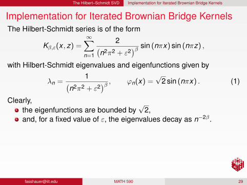
Implementation for Iterated Brownian Bridge KernelsThe Hilbert-Schmidt series is of the form
Kβ,ε(x , z) =∞∑
n=1
2(n2π2 + ε2
)β sin (nπx) sin (nπz) ,
with Hilbert-Schmidt eigenvalues and eigenfunctions given by
λn =1(
n2π2 + ε2)β , ϕn(x) =
√2 sin (nπx) . (1)
Clearly,the eigenfunctions are bounded by
√2,
and, for a fixed value of ε, the eigenvalues decay as n−2β.
Therefore, in Chapter 6 we decided to use the truncation length
M(β, ε; εmach) =
⌈1π
√ε−1/βmach (N2π2 + ε2)− ε2
⌉,
where dxe denotes the smallest integer greater than or equal to x (theceiling of x).
[email protected] MATH 590 29

The Hilbert–Schmidt SVD Implementation for Iterated Brownian Bridge Kernels
Implementation for Iterated Brownian Bridge KernelsThe Hilbert-Schmidt series is of the form
Kβ,ε(x , z) =∞∑
n=1
2(n2π2 + ε2
)β sin (nπx) sin (nπz) ,
with Hilbert-Schmidt eigenvalues and eigenfunctions given by
λn =1(
n2π2 + ε2)β , ϕn(x) =
√2 sin (nπx) . (1)
Clearly,the eigenfunctions are bounded by
√2,
and, for a fixed value of ε, the eigenvalues decay as n−2β.Therefore, in Chapter 6 we decided to use the truncation length
M(β, ε; εmach) =
⌈1π
√ε−1/βmach (N2π2 + ε2)− ε2
⌉,
where dxe denotes the smallest integer greater than or equal to x (theceiling of x).
[email protected] MATH 590 29

The Hilbert–Schmidt SVD Implementation for Iterated Brownian Bridge Kernels
Program (MaternQRDemo.m)N = 21; x = linspace(0,1,N)’; x = x(2:N-1);N = N-2; xx = linspace(0,1,100)’;f = @(x) .25^(-28)*max(x-.25,0).^14.*max(.75-x,0).^14; y = f(x);ep = 1; beta = 7; % DO NOT use with beta < 3 !!phifunc = @(n,x) sqrt(2)*sin(pi*x*n);lambdafunc = @(n) ((n*pi).^2+ep^2).^(-beta);M = max(N,ceil(1/pi*sqrt(eps^(-1/beta)*(N^2*pi^2+ep^2)-ep^2)));Lambda = diag(lambdafunc(1:M));Phi = phifunc(1:M,x);K = Phi*Lambda*Phi’; c = K\y;Phi_eval = phifunc(1:M,xx);y_standard = Phi_eval*Lambda*Phi’*c;Phi_1 = Phi(:,1:N); Phi_2 = Phi(:,N+1:end);Lambda_1 = Lambda(1:N,1:N); Lambda_2 = Lambda(N+1:M,N+1:M);Correction = Lambda_2*(Phi_1\Phi_2)’/Lambda_1;Psi = Phi*[eye(N);Correction];Psi_eval = Phi_eval*[eye(N);Correction];y_HS = Psi_eval*(Psi\y);plot(xx,y_standard,’linewidth’,2),hold onplot(xx,y_HS,’g’,xx,f(xx),’:r’,’linewidth’,3)
[email protected] MATH 590 30

The Hilbert–Schmidt SVD Implementation for Iterated Brownian Bridge Kernels
Standard RBF vs. HS-SVD InterpolationWe use
Kβ,ε with β = 7 and ε = 1 (known only in series form)N = 21 uniform samples of f (x) = (1− 4x)14
+ (4x − 3)14+
0 0.2 0.4 0.6 0.8 1−1
−0.5
0
0.5
1
1.5
Standard basisHS−SVDTrue solution
Note: cond(K) = 3.4× 10¹⁷
[email protected] MATH 590 31
The Hilbert–Schmidt SVD Implementation for Iterated Brownian Bridge Kernels
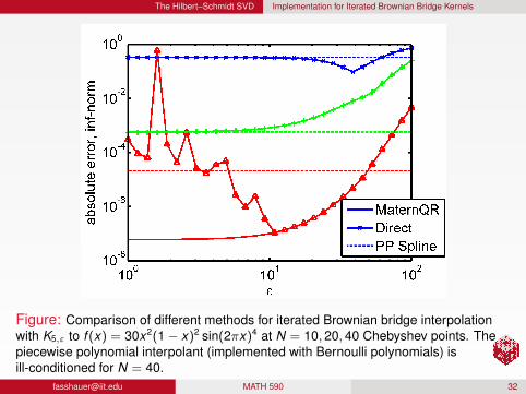
Figure: Comparison of different methods for iterated Brownian bridge interpolationwith K5,ε to f (x) = 30x2(1 − x)2 sin(2πx)4 at N = 10, 20, 40 Chebyshev points. Thepiecewise polynomial interpolant (implemented with Bernoulli polynomials) isill-conditioned for N = 40.
[email protected] MATH 590 32

The Hilbert–Schmidt SVD Implementation for Gaussian Kernels
The implementation for Gaussian kernels is much more complicated.Evaluation of the eigenfunctions
ϕn(x) =
8√
1 +(2εα
)2
√2nn!
e−(√
1+( 2εα )
2−1)α2x2
2 Hn
4
√1 +
(2εα
)2
αx
requires lots of care. The different factors of the eigenfunctionsmay become extremely large or extremely small.
To ensure safe computation of the product form of theeigenfunctions they are evaluated using logarithms.A number of asymptotic expansions are used in the GaussQRimplementation for different ranges of the argument of ϕ (see[McC13] for details).
[email protected] MATH 590 33

The Hilbert–Schmidt SVD Implementation for Gaussian Kernels
Choice of the truncation length M is not as simple as for theRBF-QR implementation with iterated Brownian bridge kernelssince the eigenfunctions are more complicated.
The global scale parameter α is an additional parameter thatneeds to be chosen carefully. It is needed to obtain theHilbert-Schmidt expansion and has a significant (not yet fullyunderstood) effect on the practical implementation of GaussQR.
[email protected] MATH 590 34

The Hilbert–Schmidt SVD Implementation for Gaussian Kernels
Choice of the truncation length M is not as simple as for theRBF-QR implementation with iterated Brownian bridge kernelssince the eigenfunctions are more complicated.The global scale parameter α is an additional parameter thatneeds to be chosen carefully. It is needed to obtain theHilbert-Schmidt expansion and has a significant (not yet fullyunderstood) effect on the practical implementation of GaussQR.
[email protected] MATH 590 34

The Hilbert–Schmidt SVD Implementation for Gaussian Kernels
Figure: The first eight Gaussian eigenfunctions with ε = 1 and α = 0.1,1,10.
Run GaussianEigenfunctions.cdf
[email protected] MATH 590 35

The Hilbert–Schmidt SVD Implementation for Gaussian Kernels
In particular, the interplay of ε, M, and α needs to be furtherinvestigated.
For higher-dimensional applicationsdifferent values of ε and α for different coordinates, i.e., anisotropickernels, can be used (but haven’t been yet),the sorting order of eigenfunctions corresponding to eigenvalues ofthe same magnitude is currently done rather arbitrarily.
[email protected] MATH 590 36

The Hilbert–Schmidt SVD Implementation for Gaussian Kernels
In particular, the interplay of ε, M, and α needs to be furtherinvestigated.For higher-dimensional applications
different values of ε and α for different coordinates, i.e., anisotropickernels, can be used (but haven’t been yet),the sorting order of eigenfunctions corresponding to eigenvalues ofthe same magnitude is currently done rather arbitrarily.
[email protected] MATH 590 36

The Hilbert–Schmidt SVD RBF-QR in Regression Mode
As an alternative to the RBF-QR algorithm which is designed toreproduce all the entries of K up to machine precision we consider twodifferent regression approaches:
using early truncation of the Hilbert-Schmidt series, i.e., a basisbuilt from the first M < N eigenfunctions, andusing a truncated Hilbert-Schmidt SVD.
RemarkThe first approach is much simpler, but data-independent. Thismay have advantages and disadvantages.The second approach requires all the work to create the matrix Ψ,but has inherently the same data-dependence as the matrix K.
We now discuss both of these.
[email protected] MATH 590 37

The Hilbert–Schmidt SVD RBF-QR in Regression Mode
As an alternative to the RBF-QR algorithm which is designed toreproduce all the entries of K up to machine precision we consider twodifferent regression approaches:
using early truncation of the Hilbert-Schmidt series, i.e., a basisbuilt from the first M < N eigenfunctions, and
using a truncated Hilbert-Schmidt SVD.
RemarkThe first approach is much simpler, but data-independent. Thismay have advantages and disadvantages.The second approach requires all the work to create the matrix Ψ,but has inherently the same data-dependence as the matrix K.
We now discuss both of these.
[email protected] MATH 590 37

The Hilbert–Schmidt SVD RBF-QR in Regression Mode
As an alternative to the RBF-QR algorithm which is designed toreproduce all the entries of K up to machine precision we consider twodifferent regression approaches:
using early truncation of the Hilbert-Schmidt series, i.e., a basisbuilt from the first M < N eigenfunctions, andusing a truncated Hilbert-Schmidt SVD.
RemarkThe first approach is much simpler, but data-independent. Thismay have advantages and disadvantages.The second approach requires all the work to create the matrix Ψ,but has inherently the same data-dependence as the matrix K.
We now discuss both of these.
[email protected] MATH 590 37

The Hilbert–Schmidt SVD RBF-QR in Regression Mode
As an alternative to the RBF-QR algorithm which is designed toreproduce all the entries of K up to machine precision we consider twodifferent regression approaches:
using early truncation of the Hilbert-Schmidt series, i.e., a basisbuilt from the first M < N eigenfunctions, andusing a truncated Hilbert-Schmidt SVD.
RemarkThe first approach is much simpler, but data-independent. Thismay have advantages and disadvantages.
The second approach requires all the work to create the matrix Ψ,but has inherently the same data-dependence as the matrix K.
We now discuss both of these.
[email protected] MATH 590 37

The Hilbert–Schmidt SVD RBF-QR in Regression Mode
As an alternative to the RBF-QR algorithm which is designed toreproduce all the entries of K up to machine precision we consider twodifferent regression approaches:
using early truncation of the Hilbert-Schmidt series, i.e., a basisbuilt from the first M < N eigenfunctions, andusing a truncated Hilbert-Schmidt SVD.
RemarkThe first approach is much simpler, but data-independent. Thismay have advantages and disadvantages.The second approach requires all the work to create the matrix Ψ,but has inherently the same data-dependence as the matrix K.
We now discuss both of these.
[email protected] MATH 590 37

The Hilbert–Schmidt SVD RBF-QR in Regression Mode
RBF-QRr
We want to use M < N eigenfunctions to produce a low-rankapproximation to the RBF interpolant based on N pieces of data.The motivation is to
eliminate high-order eigenfunctions which contribute very little tothe solution, but increase computational cost.This may reduce the sensitivity of the solution to α.In particular, experiments have shown that the choice of an“optimal” α depends on ε and is also more sensitive withincreasing M.
[email protected] MATH 590 38

The Hilbert–Schmidt SVD RBF-QR in Regression Mode
In order to introduce this problem in the same context as theinterpolatory RBF-QR we assume
that M ≤ N is fixed andset all the eigenvalues λn, n = M = 1, . . . ,N to zero.
This results in an approximate decomposition of the kernel matrix
K ≈ ΦΛΦT
=
Φ1 Φ2
(Λ10
) Φ1 Φ2
T
,
whereΦ1 is based on the first M eigenfunctions,Λ1 contains the first M (and only nonzero) eigenvalues, andΦ2 contains the remaining N −M eigenfunctions.
[email protected] MATH 590 39
The Hilbert–Schmidt SVD RBF-QR in Regression Mode
To get the new basis matrix Ψ for the RBF-QR method we had tomultiply K by M−1.
We define the matrix1 M analogously to before:
M = ΛΦT .
However, since Λ is not invertible we use its pseudoinverse (Φ is N ×Nand invertible, so we don’t need to use a QR decomposition here):
M† = Φ−T Λ† = Φ−T(
Λ−11
0
).
This means that our new basis functions are given by
ψ(x)T = k(x)T M†.
1This would have to be called a “low-rank preconditioning” matrix.
[email protected] MATH 590 40
The Hilbert–Schmidt SVD RBF-QR in Regression Mode
To get the new basis matrix Ψ for the RBF-QR method we had tomultiply K by M−1.
We define the matrix1 M analogously to before:
M = ΛΦT .
However, since Λ is not invertible we use its pseudoinverse (Φ is N ×Nand invertible, so we don’t need to use a QR decomposition here):
M† = Φ−T Λ† = Φ−T(
Λ−11
0
).
This means that our new basis functions are given by
ψ(x)T = k(x)T M†.
1This would have to be called a “low-rank preconditioning” [email protected] MATH 590 40
The Hilbert–Schmidt SVD RBF-QR in Regression Mode
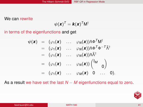
We can rewriteψ(x)T = k(x)T M†
in terms of the eigenfunctions and get
ψ(x) = (ϕ1(x) . . . ϕN(x))ΛΦT M†
= (ϕ1(x) . . . ϕN(x))ΛΦT Φ−T Λ†
= (ϕ1(x) . . . ϕN(x))ΛΛ†
= (ϕ1(x) . . . ϕN(x))
(IM
0
)= (ϕ1(x) . . . ϕM(x) 0 . . . 0).
As a result we have set the last N −M eigenfunctions equal to zero.
[email protected] MATH 590 41

The Hilbert–Schmidt SVD RBF-QR in Regression Mode
We can rewriteψ(x)T = k(x)T M†
in terms of the eigenfunctions and get
ψ(x) = (ϕ1(x) . . . ϕN(x))ΛΦT M†
= (ϕ1(x) . . . ϕN(x))ΛΦT Φ−T Λ†
= (ϕ1(x) . . . ϕN(x))ΛΛ†
= (ϕ1(x) . . . ϕN(x))
(IM
0
)
= (ϕ1(x) . . . ϕM(x) 0 . . . 0).
As a result we have set the last N −M eigenfunctions equal to zero.
[email protected] MATH 590 41

The Hilbert–Schmidt SVD RBF-QR in Regression Mode
We can rewriteψ(x)T = k(x)T M†
in terms of the eigenfunctions and get
ψ(x) = (ϕ1(x) . . . ϕN(x))ΛΦT M†
= (ϕ1(x) . . . ϕN(x))ΛΦT Φ−T Λ†
= (ϕ1(x) . . . ϕN(x))ΛΛ†
= (ϕ1(x) . . . ϕN(x))
(IM
0
)= (ϕ1(x) . . . ϕM(x) 0 . . . 0).
As a result we have set the last N −M eigenfunctions equal to zero.
[email protected] MATH 590 41
The Hilbert–Schmidt SVD RBF-QR in Regression Mode
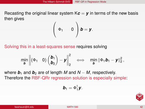
Recasting the original linear system Kc = y in terms of the new basisthen gives Φ1 0
b = y .
Solving this in a least-squares sense requires solving
minb
∥∥∥∥(Φ1 0)
(b1b2
)− y
∥∥∥∥2
2⇐⇒ min
b‖Φ1b1 − y‖22 ,
where b1 and b2 are of length M and N −M, respectively.Therefore the RBF-QRr regression solution is especially simple:
b1 = Φ†1y .
[email protected] MATH 590 42

The Hilbert–Schmidt SVD RBF-QR in Regression Mode
Recasting the original linear system Kc = y in terms of the new basisthen gives Φ1 0
b = y .
Solving this in a least-squares sense requires solving
minb
∥∥∥∥(Φ1 0)
(b1b2
)− y
∥∥∥∥2
2⇐⇒ min
b‖Φ1b1 − y‖22 ,
where b1 and b2 are of length M and N −M, respectively.
Therefore the RBF-QRr regression solution is especially simple:
b1 = Φ†1y .
[email protected] MATH 590 42
The Hilbert–Schmidt SVD RBF-QR in Regression Mode
Recasting the original linear system Kc = y in terms of the new basisthen gives Φ1 0
b = y .
Solving this in a least-squares sense requires solving
minb
∥∥∥∥(Φ1 0)
(b1b2
)− y
∥∥∥∥2
2⇐⇒ min
b‖Φ1b1 − y‖22 ,
where b1 and b2 are of length M and N −M, respectively.Therefore the RBF-QRr regression solution is especially simple:
b1 = Φ†1y .
[email protected] MATH 590 42
The Hilbert–Schmidt SVD RBF-QR in Regression Mode
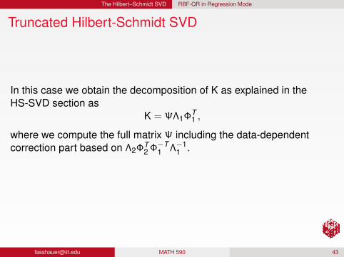
Truncated Hilbert-Schmidt SVD
In this case we obtain the decomposition of K as explained in theHS-SVD section as
K = ΨΛ1ΦT1 ,
where we compute the full matrix Ψ including the data-dependentcorrection part based on Λ2ΦT
2 Φ−T1 Λ−1
1 .
The truncated Hilbert-Schmidt SVD then zeros eigenvalues in Λ1.
[email protected] MATH 590 43
The Hilbert–Schmidt SVD RBF-QR in Regression Mode
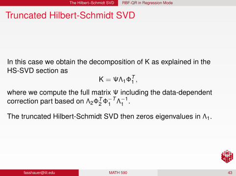
Truncated Hilbert-Schmidt SVD
In this case we obtain the decomposition of K as explained in theHS-SVD section as
K = ΨΛ1ΦT1 ,
where we compute the full matrix Ψ including the data-dependentcorrection part based on Λ2ΦT
2 Φ−T1 Λ−1
1 .
The truncated Hilbert-Schmidt SVD then zeros eigenvalues in Λ1.
[email protected] MATH 590 43

Implementation Issues in Higher Dimensions
Outline
1 Introduction
2 Contour-Padé – The First Stable Algorithm
3 The Hilbert–Schmidt SVD
4 Implementation Issues in Higher Dimensions
[email protected] MATH 590 44

Implementation Issues in Higher Dimensions
If we want to move to higher dimensions, then using kernels in productform is most advantageous.
ExampleGaussian kernel
where
λn =d∏`=1
λn` , ϕn(x) =d∏`=1
ϕn`(x`).
Different shape parameters ε` (and different α`) for different spacedimensions are allowed (i.e., K may be anisotropic).
[email protected] MATH 590 45

Implementation Issues in Higher Dimensions
If we want to move to higher dimensions, then using kernels in productform is most advantageous.
ExampleGaussian kernel
K (x , z) = e−ε2‖x−z‖2
2 = e−
d∑=1ε2(x`−z`)2
=d∏`=1
e−ε2(x`−z`)2
x = (x1, . . . , xd ) ∈ Rd ,
where
λn =d∏`=1
λn` , ϕn(x) =d∏`=1
ϕn`(x`).
Different shape parameters ε` (and different α`) for different spacedimensions are allowed (i.e., K may be anisotropic).
[email protected] MATH 590 45

Implementation Issues in Higher Dimensions
If we want to move to higher dimensions, then using kernels in productform is most advantageous.
ExampleGaussian kernel
K (x , z) = e−ε2‖x−z‖2
2 = e−
d∑=1ε2`(x`−z`)2
=d∏`=1
e−ε2`(x`−z`)2
x = (x1, . . . , xd ) ∈ Rd ,
where
λn =d∏`=1
λn` , ϕn(x) =d∏`=1
ϕn`(x`).
Different shape parameters ε` (and different α`) for different spacedimensions are allowed (i.e., K may be anisotropic).
[email protected] MATH 590 45
Implementation Issues in Higher Dimensions
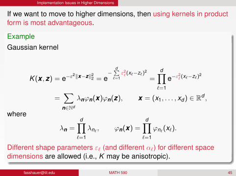
If we want to move to higher dimensions, then using kernels in productform is most advantageous.
ExampleGaussian kernel
K (x , z) = e−ε2‖x−z‖2
2 = e−
d∑=1ε2`(x`−z`)2
=d∏`=1
e−ε2`(x`−z`)2
=∑
n∈Nd
λnϕn(x)ϕn(z), x = (x1, . . . , xd ) ∈ Rd ,
where
λn =d∏`=1
λn` , ϕn(x) =d∏`=1
ϕn`(x`).
Different shape parameters ε` (and different α`) for different spacedimensions are allowed (i.e., K may be anisotropic).
[email protected] MATH 590 45


Implementation Issues in Higher Dimensions
In higher dimensions there will be multiple eigenvalues of the sameorder, and therefore ordering of eigenvalues and their associatedeigenfunctions may matter for the performance of the algorithm.
Using product kernels [FM12] (with uniform ε and α) eigenvaluesof the same order follow Pascal’s triangle. E.g., in threedimensions the first eigenvalues λ1, λ2, λ3, λ4, take the form
λ0,0,0
λ1,0,0, λ0,1,0, λ0,0,1
λ2,0,0, λ1,1,0, λ1,0,1, λ0,2,0, λ0,1,1, λ0,0,2
λ3,0,0, λ2,1,0, λ2,0,1, λ1,2,0, λ1,1,1, λ1,0,2, λ0,3,0, λ0,2,1, λ0,1,2, λ0,0,3
Since we may want to use only the “first”, e.g., 12 eigenfunctions weneed to decide which two of the order three eigenvalues are mostsignificant.
[email protected] MATH 590 48

Implementation Issues in Higher Dimensions
Fornberg, Larsson and Flyer [FLF11] reported several othereigenvalue patterns for their kernels:
In 2D for Gaussians, MQs, IMQs, IQs and Bessel kernels withβ > d = 2 we have multiplicities
1, 2, 3, 4, 5, 6, 7, . . .
In 2D for Bessel kernels with β = d = 2 we have multiplicities
1, 2, 2, 2, 2, 2, 2, . . .
In 3D for Gaussians (see above), MQs, IMQs and IQs we havemultiplicities
1, 3, 6, 10, 15, 21, 28, . . .
On the sphere S2 [FP08] for Gaussians, MQs, IMQs and IQs wehave multiplicities
1, 3, 5, 7, 9, 11, 13, . . .
[email protected] MATH 590 49

Appendix References
References I
[BLB01] R. K. Beatson, W. A. Light, and S. Billings, Fast solution of the radial basisfunction interpolation equations: domain decomposition methods, SIAMJournal on Scientific Computing 22 (2001), no. 5, 1717–1740.
[CFM14] Roberto Cavoretto, G. E. Fasshauer, and M. J. McCourt, An introduction tothe Hilbert-Schmidt SVD using iterated Brownian bridge kernels, NumericalAlgorithms (2014).
[Fas07] G. E. Fasshauer, Meshfree Approximation Methods with MATLAB,Interdisciplinary Mathematical Sciences, vol. 6, World Scientific PublishingCo., Singapore, 2007.
[Fas11a] , Green’s functions: taking another look at kernel approximation,radial basis functions and splines, Approximation Theory XIII: San Antonio2010 (M. Neamtu and L. L. Schumaker, eds.), Springer Proceedings inMathematics, vol. 13, Springer, 2011, pp. 37–63.
[Fas11b] , Positive definite kernels: past, present and future, DolomitesResearch Notes on Approximation 4 (2011), 21–63.
[email protected] MATH 590 50
Appendix References
References II
[FLF11] Bengt Fornberg, Elisabeth Larsson, and Natasha Flyer, Stablecomputations with Gaussian radial basis functions, SIAM Journal onScientific Computing 33 (2011), no. 2, 869–892.
[FM12] G. E. Fasshauer and M. J. McCourt, Stable evaluation of Gaussian radialbasis function interpolants, SIAM J. Sci. Comput. 34 (2012), no. 2,A737—A762.
[FP08] B. Fornberg and C. Piret, A stable algorithm for flat radial basis functions ona sphere, SIAM J. Sci. Comput. 30 (2008), no. 1, 60–80.
[FW04] B. Fornberg and G. Wright, Stable computation of multiquadric interpolantsfor all values of the shape parameter, Comput. Math. Appl. 48 (2004),no. 5–6, 853–867.
[GRZ13] M. Griebel, C. Rieger, and B. Zwicknagl, Multiscale approximation andreproducing kernel Hilbert space methods, 2013.
[McC13] M. McCourt, Building infrastructure for multiphysics simulations, Ph.D.thesis, Cornell University, 2013.
[email protected] MATH 590 51
Appendix References
References III
[Sch81] L. L. Schumaker, Spline functions: Basic theory, John Wiley & Sons (NewYork), 1981, reprinted by Krieger Publishing 1993.
[Tre13] Lloyd N. Trefethen, Approximation Theory and Approximation Practice,SIAM, 2013.
[Wri03] G. B. Wright, Radial basis function interpolation: Numerical and analyticaldevelopments, Ph.d. thesis, University of Colorado at Boulder, 2003.
[email protected] MATH 590 52