math 60082 computational finance
TRANSCRIPT

MATH 60082 Computational Finance
Dr Paul Johnson
Semester 2 – 2018
LECTURE: Monday 11:00am - 12:00pm Ellen Wilkinson Building A2.16
LAB CLASS: Thursday 12:00pm - 14:00pm Turing Ground Floor G-105
OFFICE HOURS: Tuesday 10:30-11:30am (check website)
CONTACT DETAILS: Office - 2.107 Turing Building
Direct tel - (0161 30)63660E-mail - [email protected] - http://www.maths.manchester.ac.uk/∼pjohnson
ASSESSMENT:
This course is entirely assessed by project work. There will be five assignments in total, withtwo short mini tasks accounting for 5%, and three main assignments each of which will ac-count for 30% of your final mark for this module. I will attempt to spread these as evenlythroughout the semester; I will allow at least three weeks (for main assignments) between giv-ing out project details and the date to be handed in. DEADLINES MUST BE STRICTLY
OBSERVED!!!
IMPORTANT DATES:
Support Computing Class 14:00pm - 17:00pm Wednesday 1st February 2017 - AT G.105Mini Task 1 Sunday 11th February 2018
Mini Task 2 Sunday 18th February 2018
Main Assignment 1 Sunday 11th March 2018
Main Assignment 2 Friday 20th April 2018
Last Lecture Monday 23rd April 2018Main Assignment 3 Sunday 6th May 2018
RECOMMENDED TEXTS:
There are a number of texts on Computational Finance; most are fairly awful. Other texts onmore general aspects of the subject are good on some areas of Computational Finance, but noton others. Here are some suggestions:
Text books:
1
• A good basic text for Mathematical Finance (also useful for MATH 39032/60008) is:
Wilmott, P., Howison, S., Dewynne, J., 1995: The Mathematics of Financial Derivatives,Cambridge U.P. ISBN: 0521497892
• Alternatively, as an introductory text to the area:
Wilmott, P., 2001: Paul Wilmott Introduces Quantitative Finance, 2nd Edition, Wiley.ISBN: 0471498629.
• For a very detailed (and expensive) look at mathematical finance:
Wilmott, P., 2000: Paul Wilmott on Quantitative Finance, Wiley. ISBN: 0471874388
• For a more financial look at options and derivatives the following is excellent and is thecourse text for finance students (usually MBA or PhD) studying derivatives (with a decenttreatment of binomial trees):
Hull, J. C., 2002: Options, Futures and other Derivatives, 5th edition, Prentice Hall.ISBN: 0130465925.
• For a readable book on Stochastic Finance (including a good treatment of Monte Carlomethods):
Higham, D.J. 2004: An introduction to financial option valuation. Cambridge UniversityPress. ISBN 0521 54757 1 for paperback and ISBN 0521 83884 3 for hardback.
• For a book which describes numerous computational routines
William H. Press, Brian P. Flannery and Saul A. Teukolsky 1992 Numerical Recipes in C:the art of scientific computing Cambridge University Press. ISBN-10: 0521431085 (thereare also FORTRAN and C++ versions of this book).
• For a great book on the numerical solution of PDEs (written long before CF was invented!)
G. D. Smith, 1986 Numerical Solution of Partial Differential Equations Oxford UniversityPress. ISBN10: 0198596502
• For an excellent book for programing using C++
M. Joshi, 2004 C++ Design Patterns and Derivatives Pricing. Cambridge UniversityPress. ISBN 0 521 83235 7
2

1 Introduction
Important - always remember:
Garbage in, garbage out
- this is the golden rule of computing!
1.1 Introduction
In this course we will be studying computational finance (or CF). Whilst basic financialmathematics problemsmay have analytical solutions (which even then may ultimately require anelement of computation, such as the evaluation of special functions - see below), most real financeproblems rely heavily on numerical (i.e. computational) techniques. Indeed, the calculation ofthe values of early exercise (e.g. American) options is inherently nonlinear, and as a consequencethese must be tackled numerically.
The aim of the course is to give a broad outline of the main numerical techniques employedin the finance world. The list, in chronological order is:
• ‘Exact’ solutions - evaluation of the Black-Scholes formula
• Lattice (tree) methods
• Quadrature methods
• Monte Carlo methods
• Methods for partial differential equations (PDEs) - finite difference methods
Throughout the emphasis will be on a critical appraisal of methods, especially accuracy (i.e.errors).
The different types of errors can be categorised into the following main types:
• Roundoff errors
• Truncation and discretization errors
• Errors in modelling
• AND THE MOST IMPORTANT FOR BEGINNERS: Programming errors
Let us consider these in turn:
1.2 Roundoff errors
These arise when a computer is used for doing numerical calculations. Some typical exam-ples include the inexact representation of (e.g. irrational) numbers such as π,
√2. Roundoff
and chopping errors arise from the way numbers are stored on the computer, and in the wayarithmetic operations are carried out. Whereas most of the time the numbers are stored on acomputer is not under our control, the way certain expressions are computed definitely is. Asimple example will illustrate the point. Consider the computation of the roots of a quadraticequation ax2 + bx+ c = 0 with the expressions
x1 =−b+
√b2 − 4ac
2a, x2 =
−b−√b2 − 4ac
2a
3

Let us take a = c = 1, b = −28. Then x1 = 14 +√195, x2 = 14 −
√195. Now to 5 significant
figures we have√195 = 13.964. Hence x1 = 27.964, x2 = 0.036. So what can we say about the
error? We need some way to quantify errors. There are two useful measures for this.
Absolute error
Suppose that φ∗ is an approximation to a quantity φ. Then the absolute error is defined by|φ∗ − φ|.
Relative error
Another measure is the relative error and this is defined by |φ∗ − φ|/|φ| if φ 6= 0.For our example above we see that |x∗1 − x1| = 2.4 ∗ 10−4 and |x∗2 − x2| = 2.4 ∗ 10−4
which look small. On the other hand the relative errors are |x∗1 − x1|/|x1| = 8.6 ∗ 10−6 and|x∗2 − x2|/|x2| = 6.7 ∗ 10−3. Thus the accuracy in computing x2 is far less than in computingx1. On the other hand if we compute x2 via
x2 = 14−√195 =
1
14 +√195
we obtain x2 = 0.03576 with a much smaller absolute error of 3.4 ∗ 10−7 and a relative error of9.6 ∗ 10−6.
Note that roundoff error can be reduced by performing arithmetic operations at higherprecision (i.e. more significant figures).
1.3 Truncation and discretization errors
These errors arise when we take the continuum model and replace it with a discrete approx-imation. For example suppose we wish to solve
d2U
dx2= f(x),
using Taylor series (more details later) we can approximate the second derivative term by
U(xi+1)− 2U(xi) + U(xi−1)
h2
where we consider a set of x points xi = x0+i∗h, i = 1, 2, . . ., where we have taken a uniform gridwith spacing h say and node points xi. As far the approximation of the equation is concernedwe will have a truncation error given by
τ(xi) =d2U(xi)
dx2− f(xi) =
h2
12
d4U
dx4+ . . .
Even though the discrete equations may be solved to high accuracy, there will be still anerror of O(h2) arising from the discretization of the equations. Of course with more points, wewould expect this error to diminish.
4

1.4 Errors in modelling
These arise for example when the equations being solved are not the proper equationsfor the problem. For example the Black Scholes equation has a number (many) underlyingassumptions (some of which can be relaxed, others of which are still open to question). Nomatter how accurately the solution has been computed, it may not be close to the real solutionbecause other factors have been neglected in the computation. This class of error is not dealtwith in this course, but you should always be aware of the limitations of the model you areusing.
1.5 Programming errors (bugs)
These are errors entirely under the control of the programmer. To eliminate these requirescareful testing of the code and logic, as well as comparison with previous work. It is alwaysuseful to have benchmarks - for example an exact solution may exist (sometimes), or previouswork with which it is possible to compare your numerical results. However for your problem forwhich there may not be previous work to compare with, one has to do numerous self-consistencychecks with further analysis as necessary.
1.6 Benchmarking
As mentioned above, if you are lucky enough to have an exact solution with which to compareyour numerical results - use it!
Consider the Black Scholes PDE (this has been/will be derived in other modules)
∂V
∂t+
1
2σ2S2∂
2V
∂S2+ rS
∂V
∂S− rV = 0.
Here V denotes the value of the option, S that of the underlying, t time, σ the volatilityand r risk-free interest rate.
For the case of a European call option (final condition C(t = T ) = max(S−X, 0)), the priceis
C(S, t) = SN(d1)−Xe−r(T−t)N(d2)
whilst for a European put option (final condition P ((t = T ) = max(X − S, 0)), the price is
P (S, t) = Xe−r(T−t)N(−d2)− SN(−d1)
where
d1 =log(S/X) + (r + 1
2σ2)(T − t)
σ√T − t
,
d2 =log(S/X) + (r − 1
2σ2)(T − t)
σ√T − t
.,
and
N(x) =1√2π
∫ x
−∞e−
12s2ds
which we recognise as the cumulative distribution function for a Normal distribution. This isan example of the need to undertake a calculation, even when an analytic solution exists.
5

2 Euler’s method - a simple procedure for ODEs
This method is a major component of Monte Carlo simulations!Consider the initial value problem
dy
dx= f(x, y), a ≤ x ≤ b,
subject to the initial condition y(a) = α.Note that this formulation also encompasses nonlinear ODEs.Using a Taylor series expansion of y(x+ h) about y(x) we obtain
y(x+ h) = y(x) + hdy
dx(x) + 1
2h2 d
2y
dx2(x) + . . .
Rearranging this, we obtain
dy
dx(x) =
y(x+ h)− y(x)
h− 1
2hd2y
dx2(x) + . . .
Substituting this into our ODE, neglecting the O(h) terms leads to
y(x+ h)− y(x)
h≈ f(x, y(x))
ory(x+ h) ≈ y(x) + hf(x, y(x)).
Given y(x = a) = α, this gives us a recipe for progressing the solution forwards in x. This isa marching/stepping process, with the solution obtained at x = a+ h (from x = a), x = a+2h(from x = a+ h), ... x = a+ ih (from x = a+ (i− 1)h), etc.
Advantages of the method
• It is simple (and also simple to program)
• It is robust
• h can be changed from step to step
Disadvantages of the method
• It is not very accurate
In general we say that a method is of order hp if the error is of order hp. In principle ifh decreases, we should be able to achieve greater accuracy, although in practise roundoff errorlimits the smallest size of h that we can take. Euler’s method is first-order accurate. Higherorder schemes certainly exist, but Euler’s method is certainly the most popular with financialpractitioners using Monte Carlo simulations.
6

3 Monte Carlo methods
3.1 Introduction
• We now look at a numerical scheme that uses the probabilistic solution - Monte Carlotechniques.
• The main idea behind the Monte Carlo technique is that you simulate paths that couldbe taken by the underlying asset (under the risk-neutral probability) and then use theseto estimate an expected option price at expiry, which can be discounted back to today.
• Monte Carlo techniques are very useful for options on more than one underlying asset.
• Sadly, the convergence of Monte Carlo methods is slow and it is hard to determine theerror terms.
• The convergence to the correct option value will be at a rate of N−12 where N is the
number of sample paths.
• As it is a forward induction technique, which makes it particularly suitable for valuingpath dependent options such as lookback and Asian options.
• It is very unsuitable for valuing American style options for exactly the same reasons,although we shall see methods for overcoming this.
• The computational effort increases linearly as you add underlying assets, thus to pricean option with d underlying assets (or sources of uncertainty such as stochastic volatil-ity or stochastic interest rates) then an N sample paths Monte Carlo method requiresapproximately Nd calculations.
• Practitioners love these methods!!
3.2 Large numbers
• If we have a sequence of independent, identically distributed random variables Yn then wehave that
limN→∞
1
N
N∑
n=1
Yn = E[Y1]
which is the law of large numbers.
• In other words the expectation is exactly like taking a long run average (exactly as we’dexpect), so to evaluate the expectation to any desired accuracy we can simply take moreand more draws of Yn.
• With the Monte Carlo technique what we are trying to do is to evaluate the value ofE[f(YT )] which is the expectation of a function of a random variable YT .
7

3.3 Application to options
• If we consider St as the value of a share price at time t, then the option value at expiry,t = T we can think of as V (ST , T ) and from the fundamental theorem of finance we knowthat
V (St, t) = EQt [e
−∫ T
tr(s)dsV (ST , T )]
ore−r(T−t)EQ
t [V (ST , T )]
if r is constant, where Q is the risk-neutral measure and Et denotes taking the expectationat time t.
• Thus if we can estimate the expectation on the right hand side then we can simply discountthis value at the risk-free rate to obtain the option price today. In fact, with Monte-Carlomethods it is also fairly straightforward to factor in stochastic interest rates as well.
3.4 Simple example with GBM
• If we assume that we are in the risk-neutral world and the underlying asset follows geo-metric Brownian motion, thus, under the real-world measure
dSt = µStdt+ σStdX
and under the risk-neutral measure
dSt = rStdt+ σStdW
where W and X are both Brownian motions under the respective measures.
• The above stochastic differential equation can be solved exactly to yield:
ST = St exp[(r − 12σ
2)(T − t) + σdW ]
or
ST = St exp[(r − 12σ
2)(T − t) + σφ√T − t]
where φ here is a variable drawn at random from a Normal distribution with a mean of 0and a variance of 1, N(0, 1).
• To estimate the expected option value at time T , V (ST ) then we take random draws fromthe N(0, 1) distribution which enables us to calculate ST and then calculate V (ST ). Toget an approximation of the expectation we then average V (ST ).
• Thus if the nth draw from the normal distribution gives V n(ST ) then by the law of largenumbers:
1
N
N∑
n=1
V (SnT ) → EQ
t [V (ST )] as N → ∞
• Now if we define the error from the nth sample path as ǫn so
ǫn = V (SnT )− EQ
t [V (ST )]
8

3.5 Central limit theorem and error
• The Central Limit Theorem tells us that for large N if the individual errors ǫn havevariance ν = var(ǫn) (which is the same for all n) then the error when approximating theexpectation:
1
N
N∑
n=1
V (SnT )− EQ
t [V (ST )]
is approximately normally distributed with mean zero and variance ν/N and standard
deviation (ν/N)12 .
• Sadly this error bound is difficult to estimate as it is probabilistic, in that we only knowthe distribution of the errors rather than their actual values.
• Also the standard deviation of the error only declines with the square root of the numberof paths N .
• For each individual path the error will be random, depending upon the draw of φ.
• This implies we are unable to use extrapolation techniques since the errors will not bemonotonic
3.6 The Monte-Carlo method for European options
• That gives the basics of the Monte Carlo method, it is very simple to implement for manydifferent types of options.
• For a European call option the payoff at maturity V (ST ) is given by
V (ST ) = max(ST −X, 0)
and so, to value the option one simulates N possible values or paths for ST by making Nindependent draws from N(0, 1) then to use these possible values, call them φn we havefor 1 ≤ n ≤ N
SnT = St exp[(r − 1
2σ2)(T − t) + σφn
√T − t]
V (SnT ) = max(Sn
T −X, 0)
V (St, t) = e−r(T−t) 1
N
N∑
n=1
V (Snt )
3.7 Valuing Asian options
• An Asian option is an option whose payoff is a function of the average price of the un-derlying asset over the lifetime of the option. The share price is observed at M pointsin time (every day, every trading day, every week etc.) and the average is calculated byusing either geometric or arithmetic averaging.
• Consider an Asian option whose payoff is
V (T ) = max(A− S, 0)
9

where
A =1
M
M∑
i=1
S(ti)
and S(ti) are the share prices at the M sampling times t1, ..., tM .
• We need to modify our Monte-Carlo method slightly to deal with this.
• From the solution to the SDE we know that
Sti = St exp[(r − 12σ
2)(ti − t) + σ(W (ti)−W (t))]
Sti−1 = Sti exp[(r − 12σ
2)(ti+1 − ti) + σ(W (ti−1)−W (ti))]
and so the procedure is as follows:
– Simulate each of the M increments dWi by drawing φi from the Normal distributionand use
Snti = Sn
ti−1exp[(r − 1
2σ2)(ti − ti−1) + σ
√
ti − ti−1φi]
to estimate the underlying asset values at each time.
– Calculate the value of An and the payoff max(An −X, 0)
• Then repeat this procedure N times to get the option value:
V (t) = e−r(T−t) 1
N
N∑
n=1
max(An −X, 0)
• Note that here, we need to break up the path of St into M time steps and then use theN created paths to take the average.
3.8 Generating (Pseudo-)Random Numbers
• Many statistical packages have (normal) random number generators
• Otherwise, generate Normal random numbers by:
– generating random numbers that are uniformly distributed on [0, 1].
– Transforming them to obtain normally distributed random numbers
• Most straightforward way: - let F−1 denote inverse of Normal distribution function
• If x is uniformly distributed on [0, 1], then y = F−1(x) is a standard variable from thenormal distribution.
• If you have function F−1 then this is easy. For example, in Excel:-
– Has function RAND() which generates a random number uniformly distributed on[0, 1]
– Has function F−1, called NORSINV ()
10

– Thus, function call NORSINV(RAND()) returns a realisation of a standard normalrandom variable
• Disadvantage: F−1 is not known in closed form, so this approach is not always fast.
• The other issue is that these are only ”pseudo” random numbers in that the computerprogram typically has an algorithm for calculating the ‘random numbers’ , as John vonNeumann said in 1951 ”Anyone who considers arithmetical methods of producing random
digits is, of course, in a state of sin”.
• There are many alternatives (The ”Recipe” books of Press, Teuklovsky, Vetterling andFlannery are a good source, and have a good discussion of the problem), such as theMid-Square method, Congruential generation or the popular Mersenne twister...
3.9 The Box-Muller method
• The simplest technique for generating ‘decent’ Normally distributed random numbers(according to Wilmott) is the Box-Muller method which takes any uniformly distributedvariables (from any source you prefer) and turns them into Normally distributed ones.
• Given two uniformly distributed random numbers x1, x2, two Normally distributed ran-dom numbers, y1 and y2 are given by:
y1 = cos(2πx2)√
−2 log(x1), y2 = sin(2πx1)√
−2 log(x2)
3.10 More General Problems
• The two examples we talked about above - BSM setup (geometric Brownian motion) areparticularly easy because increments to logS are normally distributed or alternatively wecan write the solution to the SDE out explicitly in terms of the Normal distribution
• What do we do for non-Normal stochastic processes?
• Previously we introduced the SDE,
dSt = µStdt+ σStdX;
we first introduced a process
Sr+δt = St + µStδt+ σStφ√δt
where δt a small increment of time and φ a Normal r.v.
• The second process is more than a way to explain the first process
– Use Euler scheme to approximate the SDE
– Letting Sδtt denote the value of the Euler process at time t using an increment of δt
, Sδtt → St in the sense of mean square.
11

3.11 Stochastic volatility
• The Euler approximation is useful for processes that are not normal, i.e. something otherthan GBM
• Example: A stochastic volatility model. Under Q, we have
dSt = rStdt+ σtStdW1
dσt = (a− bσt)dt+ vρσtdW1 + vσt√
1− ρ2dW3
• Here
– a, b, v, r, ρ are constants,
– σ and S are stochastic processes
– σ(t) is interpreted as volatility at time t
• Consider M + 1 equally spaced times t0, t1, ..., tM , where δt = ti − ti−1.
• Euler approximation is
Sti = Sti−1 + rSti−1δt+ σti−1Sti−1φ1i
√δt
σti = σti−1 + (a− bσti−1)δt+ vρσti−1φ1i
√δt+ vσti−1
√
1− ρ2φ2i
√δt
where the φki (k = 1, 2) are independent standard normal r.v.’s.
• Only change from before is that we now do simulation using Euler approximation - wemust compute values at intermediate timesteps (GBM is special - SDE can be integrated‘exactly’).
3.12 Two underlying assets
• If we have two correlated underlying assets such that
dS1 = µ1S1dt+ σ1S1dX1
dS2 = µ2S2dt+ σ2S2dX∗2
whereX∗
2 = ρX1 +√
1− ρ2X2
or changing the notation slightly
dS1 = µ1S1dt+ σ1S1dX1
dS2 = µ2S2dt+ σ2ρS2dX1 + σ2√
1− ρ2S2dX2
then it is very straightforward to value an option whose payoff depends upon both of theasset prices at expiry.
• Consider an option where V (T ) = max(S1 −X1, S2 −X2, 0). So
V (t) = e−r(T−t)EQt [V (T )]
12

• Under risk-neutrality we have
dS1 = rS1dt+ σ1S1dX1
dS2 = rS2dt+ σ2ρS2dX1 + σ2√
1− ρ2S2dX2
thus from solving the SDEs
Sn1T = Sn
1t exp[(r − 12σ
21)(T − t) + σ1
√T − tφ1n]
Sn2T = Sn
2t exp[(r − 12σ
22)(T − t) + σ2ρ
√T − tφ1n + σ2
√
1− ρ2√T − tφ2n]
• So to value the equations simulate 2N draws of normally distributed random numbersand then determine the possible values of V (T ) and then discount the average
• Thus the option value can be estimated as follows:
V (t) = e−r(T−t)EQt [V (T )] =
1
N
N∑
n=1
max(Sn1t −X1, S
n2t −X2, 0)
• One question, however, is how to get the general form of the set of SDEs when we havemore than one underlying asset.
• The way in which we typically see correlation matrices (in two underlying assets) are interms of the covariance matrix of continuously compounded returns, i.e. log(Si(T )/Si(t))and this matrix is typically of the form
(
σ21 ρσ1σ2
ρσ1σ2 σ22
)
• We can write our two SDEs as follows:(
dS1t
dS2t
)
=
(
rS1t
rS2t
)
dt+
(
σ1S1t 0
σ2ρS2t σ2√
1− ρ2S2t
)(
dW1t
dW2t
)
• It so happens that the matrix, M , here
(
σ1 0
ρσ2 σ2√
1− ρ2
)
is the square root of the covariance matrix, Σ
(
σ21 ρσ1σ2
ρσ1σ2 σ22
)
in that Σ = MMT
• To check note that
(
σ1 0
ρσ2 σ2√
1− ρ2
)(
σ1 ρσ20 σ2
√
1− ρ2
)
=
(
σ21 ρσ1σ2
ρσ1σ2 σ22
)
13

3.13 In general
• In general, given any size of covariance matrix for any number of underlying assets it willbe possible to generate correlated normally distributed random variables.
• For a covariance matrix for two underlyings the correlated random variables, y1, y2, saywere obtained from
(
y1y2
)
= M
(
φ1
φ2
)
where M is the square root of the covariance matrix and φ are the independent Normallydistributed random variables.
• In general to create d-correlated Normally distributed variables y1, ..., yd from d uncorre-lated variables φ1, ....φd and MMT = Σ = covariance matrix, use
y1..yd
= M
φ1
.
.φd
3.14 Cholesky factorisation
• In general calculating the matrix M is fairly straightforward, one way of doing so is byusing a process called Cholesky factorisation.
• Cholesky factorisation is a special case of LU decomposition, specialised to symmetric,positive definite matrices
• See Paul Wilmott on Quantitative finance pp934-5 for the computer algorithm or alter-natively Press et al., numerical recipes in Fortran/C etc.
3.15 Basic Monte-Carlo methods - summary
• Simple to program and to understand, they are ideal for a first approximation to a deriva-tive value.
• Convergence is slow, and determined probabilistically which makes extrapolation impos-sible.
• Naturally designed for forward looking problems including path dependent derivativessuch as lookback options and Asian options.
• Good for derivatives where there are multiple sources of uncertainty, as the computationaleffort only increases linearly.
• We have introduced Monte Carlo methods which are very closely related to the proba-bilistic solution, in that you use simulation to determine an expected value for the optionin the future that can be discounted at the risk-free rate (according to the fundamentaltheorem) to obtain the value today.
• To simulate the paths we typically use the solution to the SDE or the Euler approximation,along with a decent generator of Normally distributed random variables.
14

• It is easy to apply to path dependent options and to options on more than one underlying,for these you need to know the covariance matrix and be able to ‘square root’ it by meansof Cholesky factorisation to be able to perform the simulations.
15

4 Improvements on and extensions of Monte Carlo Methods
4.1 Overview
• Here we will extend our basic theory and concentrate on some simple techniques to improvethe basic method.
• The techniques we will look at are using antithetic variables which is a very simple ad-justment, as is the control variate technique. We will mention something about momentmatching, importance sampling and low discrepancy sequences.
• Most of these are designed to reduce the variance of the error, except for low discrepancysequences which are used to improve the convergence rate.
4.2 Improving Monte Carlo
• Monte Carlo is typically the simplest numerical scheme to implement but as you will seeits accuracy and uncertain convergence is not ideal for accurate valuation.
• However, for complex problems with multiple Brownian motions it is often the onlymethod that can be used which makes it important for us to improve the accuracy ofthe standard model.
• In addition to this, when there are multiple Brownian motions AND early exercise featuresit is crucial that there is an adaptation to the Monte Carlo method that allows us tocompute an option value as it may well be the case that other numerical methods will notprovide a reasonable estimate.
4.3 Antithetic variables
• Antithetic variables or antithetic sampling is a simple adjustment to generating the φn
(1 6= n ≤ N).
• Instead of making N independent draws, you draw the sample in pairs; if the ith Normallydistributed variable is φi, then choose φi+1 to be −φi, then draw again for φi+2
• −φi is also Normally distributed and most importantly the mean of the two draws is zero,and so this ensures that the mean of the sample paths will be correct and the distributionsof draws will be symmetric.
• Thus if N = 500, 000, you only need to make 250, 000 random draws for φ and use thenegative of the draw to complete the required 500,000 values.
• This should improve the convergence as the distribution of paths is better matched to themodel, i.e. the mean of φ is zero
4.4 Control variate technique
• Control variate technique: This is explained through an example:
– We want to compute EQ[V (T )]
16

– And we can write
V (T ) = V (T )− V1(T ) + V1(T ),
where
∗ EQ[V1(T )] is known analytically
∗ and error in estimating EQ[V (T ) − V1(T )] by simulation is less than error inestimating EQ[V (T )]
– Then, a better estimate of EQ[V (T )] is the sum of
∗ The known value of EQ[V1(T )]
∗ Plus the estimate of EQ[V (T )− V1(T )]
• Consider a basket option with payoff of V (T ) = max[12S1(T ) +12S2(T )−X, 0] (assuming
the BSM framework)
• A natural choice of control variate is
V1(T ) = max[(S1(T )S2(T ))12 −K, 0]
• Why is this a good choice?
– EQ[V1(T )] is known analytically as products and powers of lognormal r.v.’s are log-normal, so this is a similar calculation to Black Scholes
– The difference V (T )− V1(T ) is relatively small, and thus a Monte Carlo estimate ofEQ[V (T )− V1(T )] will have a relatively small error
4.5 Moment matching
• One fairly simple strategy that works in a similar way to using antithetic variables iscalled moment matching.
• The typical way it is done is to ensure that the variance of the sample paths match thevariance of the required distribution (antithetic variables will automatically ensure thatthe mean and skewness match).
• Our Brownian motion modelling requires the variance of φ to be 1, so we would like thevariance of our random φ’s to share this property.
• To do this we first sample ourN φ values (requiringN/2 random numbers). Then calculate
their variance, v say, now replace all of the φ values with φ× v−12 and the variance of the
new random draws is 1, as required.
4.6 Importance sampling
• The idea behind importance sampling is that if you know that the payoff function is zerooutside of an interval [a, b] then any draw which makes ST lie outside of [a, b] is wasted.
• Ideally, you would only to sample from distributions that cause ST to lie in [a, b] and thenmultiply the result by the actual probability of ST being in this region.
17

• Recall that we have a function that turns a uniform random variable [0, 1] into a realisationof ST and so we can invert this map to find an interval [x1, x2] that is mapped onto [a, b],thus the probability of ST being in [a, b] is x2 − x1.
• Thus to compute the expectation at time T , draw variables from [0, 1], multiply by x2−x1and then add to x1 so that they are all in [x1, x2] and then convert the x value into φ asbefore and get a value of ST
• Determine the option value VT from ST and then average the option values to obtain anexpectation. Then multiply this expectation by (x2 − x1).
• For example, S0 = 100, X = 100, r = 0.05, σ = 0.2, T = 1. Consider a call option andso for [0, 100] the payoff contribution is zero. Thus we only need to sample in [100,∞).ST = 100 corresponds to a φ value of:
φ =log(100/100) − (r − 1
2σ2)
σ= −0.1
but P (φ = −0.1) = 0.461. So [0.461, 1] is the range of x values required.
• So every draw of x is multiplied by 0.539 and then added to 0.461 to obtain a φ value andthis only gives ST values greater than 100.
4.7 Low discrepancy sequences
• One of the most useful practical techniques for improving the accuracy of Monte Carlomethods is by using Low discrepancy sequences (also known as Quasi Monte Carlo meth-ods).
• The theory behind Monte Carlo techniques is that as you take more and more samplepaths then they will eventually cover the entire distribution of ST in the correct manner.
• Another way to think of this is that our random numbers drawn from [0, 1] will eventuallycover this interval in a uniform manner.
• Unfortunately, we cannot actually draw an infinite number of paths and for any size ofN it may well be the case that our ST values all cluster around particular values whilemissing out other regions of S space entirely.
• This problem becomes more pronounced as we increase the number of dimensions, d
• To overcome this problem we throw away the idea of using ‘random’ numbers at all andinstead choose a deterministic sequence of numbers that does a very good job of coveringthe [0, 1] interval.
• Note that as we have already discussed, most random number generators are deterministicto some extent and so this approach isn’t as odd as you would imagine.
• The most interesting thing about a low discrepancy series is that it can improve the
convergence of the Monte Carlo method from 1/N12 to 1/N , making the Monte Carlo
method fully competitive with binomial lattices.
• We will deal with a simple sequence here but there is an extensive literature on lowdiscrepancy series, see Jackel, Monte Carlo Methods in Finance for an excellent summary
18

4.8 The Halton Sequence
• Sobol sequences are the most common of the low discrepancy sequences, but for ease ofexplanation we will consider the Halton sequence.
• The Halton sequence is a sequence of numbers h(i; b) for i = 1, 2, ... where b is the baseand all of the numbers in the sequence are in [0, 1]. You can choose the base, let us selectbase 2.
• The Halton sequence is the reflection of the positive integers in the decimal point and isbest observed through an example:
Integers base 10 Integers base 2 Halton sequence base 2 Halton number base 101 1 1× 1
2 0.52 10 0× 1
2 + 1× 14 0.25
3 11 1× 12 + 1× 1
4 0.754 100 0× 1
2 + 0× 14 + 1× 1
8 0.125
• So 10 → 0.01 in base 2 terms.
• In general the ith integer, i, can be expressed as:
i =
m∑
j=1
ajbj−1
where b is the base and 0 ≤ aj < b. The Halton numbers are given by:
h(i; b) =m∑
j=1
ajb−j
• What is nice about the Halton sequence is that it fills the range [0, 1] gradually
• When extending to d multiple dimensions you should choose d prime bases
4.9 American options
• One of the key unanswered questions in finance is how to value options with early exercisefeatures by using a Monte Carlo method.
• Recall that the American option value V0 is
V0 = maxτ
[EQτ [e−rτ max(Sτ −X, 0)]
• The problem comes from the fact that Monte Carlo is a forward looking method. To usethe sample paths we would have to test early exercise at each point in time on each samplepath in order to determine what the optimal exercise strategy would be.
• This is incredibly time consuming and not practical, and simplistic approaches, such as theperfect foresight method where you simply choose the highest early exercise value duringthe lifetime of the option do not give acceptable approximations to the option value.
19

Graphical explanation of perfect hindsight
Graphical explanation of perfect foresight
If you follow the optimal strategy (shaded) then you should only exercise at expiry, but you can get a better payoff from exercising at t3. This is perfect foresight and does not value the option correctly• If you follow the optimal strategy (shaded) then you should only exercise at expiry, but
you can get a better payoff from exercising at t3. This is perfect hindsight and does notvalue the option correctly.
4.10 Early attempts
• Tilley (1993) made the first effort to adapt Monte Carlo methods to cope with earlyexercise features. The method involves a technique known as “bundling” where the pathsare constructed as usual and, at each timestep, they are bracketed into regions of assetprice.
• At expiry the option price is the average of the payoff from all the paths in the bundle.Working backwards through time, as the paths are known at each point it can be checkedwhether or not it was, on average, worth exercising in each bundle by comparing this tothe discounted option price from the future time step.
• There are evident shortcomings with this approach:
– first, all the paths have to be stored, which can cause computer memory problems
– more importantly the process overvalues the options.
– Crucially, it is also very difficult to extend to options on multiple underlyings (usuallythe Monte Carlo method’s advantage over other numerical techniques).
• Realising the main drawback in Tilley’s method, Barraquand and Martineau (1995)adapted his approach so that the bundling was in terms of payoff value rather than un-derlying asset value. Payoff value only has one dimension and so extension to manyunderlyings does not create any undue problems.
• However, although not requiring as much memory as Tilley’s approach, the approach stilldoes not converge to the correct value and always underestimates the option value (seeBoyle et al., 1997) and this estimation error can be serious. This approach is extended byRaymar and Zwecher (1998) but is still less effective than the following two methods.
20

• Broadie and Glasserman (1997) approach the Monte Carlo method as by creating upperand lower bounds. To create these bounds they use a ‘bushy tree effect’ to pursue sub andsuperoptimal strategies. The superoptimal strategy is obtained by creating a tree whosepossible next states are determined, by simulation, all the way to expiry.
• Then, in a similar vein to Tilley (1993) the option value at the previous time, t, is themaximum of the average of the values at t + ∆t discounted and the value from earlyexercise at t. This strategy does assume the investor has some foresight and so overvaluesthe option.
• The suboptimal procedure entails using the b possible paths at each time and, for eachpath,using the remaining b − 1 paths to determine whether the option is continued orexercised. This exercise choice is then applied the initial path one was focusing on. Allthe possible combinations are then averaged at each timestep.
• This method is shown to be suboptimal, for more details see Broadie and Glasserman(1997). These can then be combined to provide bounds for the put option value.
4.11 Broadie and Glasserman (1997)
• As usual, the computational effort increases only linearly as more underlying assets areadded. However, as the number of observation times is increased the calculations increaseexponentially, i.e with n paths, d observation dates and b branches in the tree the effortis nbd (b here is typically quite large, e.g. 50)
• Thus, to estimate the value of a continuously, or even daily, observed option involves theuse of extrapolation which is somewhat ad hoc if, as is the case here, the initial resultsare not converging at a known rate.
• There has been more recent work by Fu et al. (2001) who parametrise the early exer-cise curve by using Monte Carlo simulations and Rogers (2002) who uses a LagrangianMartingale to achieve a close upper bound on the option value.
4.12 Recent advances
• The most popular method for incorporating early exercise features in the Monte Carlomethods is by Longstaff and Schwartz (2001) which we will see in detail in later. Its appealis that it is simple to implement although there remain questions about its accuracy andefficiency.
• Another, more academically rigorous approach is the dual approach Haugh and Kogan(2004) which expresses the option pricing problem as a minimisation problem, from whicha tight upper bound on the price is calculated. Unfortunately, its calculation is oftenproblematic, although there are practical approaches to circumvent this see Andersen andBroadie (2004) for more details.
• The Carriere (1996) valuation of early exercise price for options using simulations andnon-parametric regression is also highly regarded.
4.13 Overview
• We have looked through a variety of extensions to the standard Monte Carlo in an effortto reduce the variance of the error or to improve the convergence.
21

• Most of the improvements are simple to apply such as antithetic variables and momentmatching, others are more complex such as low discrepancy sequences.
• Finally, we looked at some of the early attempts to use Monte Carlo methods to valueAmerican style options. This is a precursor to the Longstaff and Schwartz approach.
22

5 The binomial model
• A fundamental theorem of finance (in discrete time), also commonly known as The funda-
mental theorem of asset pricing, or The fundamental theorem of arbitrage pricing or Thefundamental theorem of arbitrage-free pricing: if there are no arbitrage opportunities andmarkets are complete (i.e. all assets are replicable) then there exists a unique, risk-neutral,pricing measure.
• As such we can write the value of any asset, in particular an option at time t, Vt, as
V0 =1
1 +REQ[VT ]
where R is the risk-free interest rate over time T . We can also write this in continuouslycompounded terms as
V0 = e−rTEQ[VT ]
• We can apply the same argument from time period to time period and so it is possible tohave binomial trees with multiple time steps to simulate the movement of the underlyingasset more accurately.
• As we have more steps in our tree we essentially have a binomial distribution with more andmore possible outcomes which should eventually approximate to the continuous, lognormaldistribution we saw in our continuous time pricing models such as Black-Scholes.
5.1 Basic binomial set up
• If we have a three asset world with a Bond, Bt, a Stock, St and a call option Ct, whereinterest rates are continuously compounded and the risk neutral probability of the up anddown states occurring are q and (1− q) then we have
B0 = 1
BT = erT
BT = erT
S0 = s
ST = us
ST = ds
C0 = ?
CT = max(us – X, 0)
CT = max(ds – X, 0)
q
1-q
1-q
q
23

Determining q, u and d
• As the probabilities are risk neutral we require that the expected return on the stock isthe same as that of the risk-free bond, thus
qsu+ (1− q)sd = serT
qu+ (1− q)d = erT
• We would also like to match the variance of our returns to that from the data. From ourcontinuous model we know that under the risk-neutral model
dS = rSdt+ σSdX
and we can solve this SDE to obtain
ST = s exp[(r − 12σ
2)T + σ√Tφ]
• Taking expectations we have for the continuous case:
E[ST ] = s exp(rT )
E[(ST )2] = s2 exp[(2r + σ2)T ]
and in the binomial caseE[ST ] = s(qu+ (1− q)d)
E[S2T ] = s2(qu2 + (1− q)d2)
thuserT = qu+ (1− q)d
e(2r+σ2)T = qu2 + (1− q)d2
• However, this still leaves us with one degree of freedom to determine all of q, u and dsince there are 3 unknowns and only 2 equations.
5.2 Some possible models
• The two most popular models for binomial pricing are Cox, Ross and Rubinstein (1979)(CRR for short) whose extra degree of freedom is to set
ud = 1
thus
u = eσ√T , d = e−σ
√T , q =
erT − d
u− d
• The other is Rendleman and Bartter (1979) who choose:
q =1
2
and so
u = e(r−12σ
2)T+σ√T , d = e(r−
12σ
2)T−σ√T .
24

5.3 Constructing the tree
• So now we have expressions for u and d which will ensure that the binomial tree willapproximate the continuous lognormal distribution which arises from the geometric Brow-nian motion assumptions.
• There are other ways to construct the tree if the underlying asset follows a differentstochastic process but we do not consider those here.
• Now we turn our attention to valuing a European call option before considering naturalextensions.
• The current value of the underlying asset is S0, the time to expiry is T , we have N timesteps, the continuously compounded risk-free rate is r, the volatility of the underlyingasset is σ and the exercise price of the option is X. The size of the time-step ∆t = T/N
• If we denote the value of the underlying asset after timestep i and upstate j by Sij andthe option price by Vij then we have that:
Sij = S0ujdi−j
VNj = max(S0ujdN−j −X, 0)
Vij = e−r∆t(qVi+1,j+1 + (1− q)Vi+1,j) for i < N
where q, u and d are selected according to your preferred model (CRR or alternative).
5.4 Example
• Consider a European call option where S0 = 100, X = 100, T = 1, r = 0.06, σ = 0.2.
• Choosing the CRR tree we have
u = eσ√∆t = 1.1224
d = e−σ√∆t = 0.8909
q =er∆t − d
u− d= 0.5584
• Next we show the calculation of the European call option price using 3 time steps, wherewe end up with an option value of $11.55.
5.5 American option valuation
• American options are call (put) options where it is possible to exercise early at time t toreceive St −X ((X − St) for a put)
• We will consider the American option pricing problem from different perspectives for thethree types of numerical methods. As noted already, it can be problematic to solve usingforward induction methods such as Monte Carlo techniques.
• The problem is a free boundary or optimal stopping problem where the current optionvalue Vt is given by
Vt = maxτ
EQt [e
−r(τ−t)Payoff(Sτ )]
where τ denotes the continuum of possible stopping times.
• This representation is not particularly useful when attempting to value the option.
25

t=0 t =1/3 t = 2/3 t = 1
V3,3 = 41.398
S3,3 = 141.40
V0,0 = 11.552
S0,0 = 100.00
V3,2 = 12.24
S3,2 = 112.24
V3,1 = 0
S3,1 = 89.094
V3,0 = 0
S3,0 = 70.722
V2,1 = 6.700
S2,1 = 100
V2,0 = 0
S2,0 = 79.379
V2,2 = 27.959
S2,2 = 125.98
V1,0 = 3.6675
S1,0 = 89.095
V1,1 = 18.204
S1,1 = 112.24
5.6 American options and lattices
• Obviously any rational investor would only exercise if the value from exercising is greaterthan the value from not exercising, i.e. holding the option for one more period.
• The nice thing about binomial lattices is that as we calculate backward we already knowthe value of holding the option until the next period (the continuation value) and we knowthe early exercise value (the payoff from the option) and so it is straightforward to adaptour European option pricing model to deal with American options
• Thus at each node in the tree we need to compare two values, the continuation (or hold)value, Vhij and the early exercise value Vxij to determine Vij where
Vij = Payoff(SNj) for t = T
Vhij = e−r∆t(qVi+1,j+1 + (1− q)Vi+1,j) for t < T
Vxij = Payoff(Sij) for t < T
Vij = max(Vhij , Vxij) for t < T
and Payoff is the appropriate payoff function for each option.
5.7 Example
• Consider an American put option where S0 = 100, X = 100, T = 1, r = 0.06, σ = 0.2.
• Choosing the CRR tree we have
u = eσ√∆t = 1.1224
d = e−σ√∆t = 0.8909
q =er∆t − d
u− d= 0.5584
26

• Next we show the calculation of the American put option price where we end up with anoption value of $6.099.
• The nodes in red denote that the holder of the option exercised early.
t=0 t =1/3 t = 2/3 t = 1
V3,3 = 0.000
Vx,3,3 = -41.4
Vh,3,3 = 0.000
S3,3 = 141.40
V0,0 = 6.099
Vx,0,0 = 0.00
Vh,0,0 = 6.099
S0,0 = 100.00
V3,2 = 0.000
Vx,3,2 = -12.2
Vh,3,2 = 0.000
S3,2 = 112.24
V3,1 = 10.90
Vx,3,1 = 10.90
Vh,3,1 = 0.000
S3,1 = 89.09
V3,0 = 29.28
Vx,3,0 = 29.28
Vh,3,0 = 0.000
V3,0 = 70.72
V2,1 = 4.7199
Vx,2,1 = 0.00
Vh,2,1 = 4.720
S2,1 = 100.0
V2,0 = 20.62
Vx,2,0 = 20.62
Vh,2,0 = 18.64
S2,0 = 79.38
V2,2 = 0.000
Vx,2,2 = -26.0
Vh,2,2 = 0.000
S2,2 = 125.98
V1,0 = 11.509
Vx,1,0 = 10.91
Vh,1,0 = 11.51
S1,0 = 89.094
V1,1 = 2.043
Vx,1,1 = -12.2
Vh,1,1 = 2.043
S1,1 = 112.24
5.8 Additional notes
• For American call options with no dividends it is never optimal to exercise early.
• From the lattice we can determine the early exercise region, the values of S and t forwhich you would exercise and the early exercise boundary which separates the exerciseand non-exercise regions.
• Technically what we have evaluated here is a Bermudan option, which is an Americanoption that can only be exercised on certain specified dates. However, as we have moreand more observation dates then this value will approach the American option price.
5.9 Continuous dividends
• The fundamental theorem of finance does not directly apply to dividend paying assets butit can be easily adjusted to do so.
• If St is the value of an asset at time t which pays out a continuously compounded dividendyield, δ, then consider a new asset X which is defined as
X0 = e−δtS0
at time t the S0 will have grown to Steδt and so Xt = St. Thus it will be possible to
replicate the value of an option expiring at time t by holding e−δt of the underlying asset.
27

• Thus by the fundamental theorem of finance it will be X which is priced under the risk-neutral measure given a known future
asset price St thus:
X0 = e−rtEQ0 [St]
and soS0 = e−(r−δ)tEQ
0 [St]
5.10 Lattices with continuous dividends
• Now given this slightly different calculation we have new values of u and d where
E[ST ] = s exp[(r − δ)T ]
E[(ST )2] = s2 exp[(2(r − δ) + σ2)T ]
and again you have another choice of a degree of freedom and the CRR approach gives:
u = eσ√∆t, d = e−σ
√∆t, q =
e(r−δ)∆t − d
u− d
in a tree with step size ∆t
• Thus if we consider the American put option only now when δ = 0.03 we see that thetheoretical price is now $7.32
t=0 t =1/3 t = 2/3 t = 1
V3,3 = 0.000
Vx,3,3 = -41.4
Vh,3,3 = 0.000
S3,3 = 141.40
V0,0 = 7.159
Vx,0,0 = 0.00
Vh,0,0 = 7.159
S0,0 = 100.00
V3,2 = 0.000
Vx,3,2 = -12.2
Vh,3,2 = 0.000
S3,2 = 112.24
V3,1 = 10.90
Vx,3,1 = 10.90
Vh,3,1 = 0.000
S3,1 = 89.09
V3,0 = 29.28
Vx,3,0 = 29.28
Vh,3,0 = 0.000
V3,0 = 70.72
V2,1 = 5.189
Vx,2,1 = 0.00
Vh,2,1 = 5.189
S2,1 = 100.0
V2,0 = 20.62
Vx,2,0 = 20.62
Vh,2,0 = 19.43
S2,0 = 79.38
V2,2 = 0.000
Vx,2,2 = -26.0
Vh,2,2 = 0.000
S2,2 = 125.98
V1,0 = 12.43
Vx,1,0 = 10.91
Vh,1,0 = 12.43
S1,0 = 89.094
V1,1 = 2.469
Vx,1,1 = -12.2
Vh,1,1 = 2.469
S1,1 = 112.24
• Perhaps a more realistic case is when there is a known discrete dividend payment at acertain point in time. In our example, imagine there is a known dividend, payable after2/3 of a year which is 3% of the share price.
28

• Here the fundamental theorem will hold from period to period and our values of u, d andq will remain the same as for the no dividend case but at t = 2/3, S2j → 0.97 × S2j
• This is depicted in the worked example next:
t=0 t =1/3 t = 2/3 Pre Div t = 2/3 Post Div t=1
V3,3 = 0.000
Vx,3,3 = -37.2
Vh,3,3 = 0.000
S3,3 = 137.16
V0,0 = 7.094
Vx,0,0 = 0.00
Vh,0,0 = 7.094
S0,0 = 100.00
V3,2 = 0.000
Vx,3,2 = -8.87
Vh,3,2 = 0.000
S3,2 = 108.87
V3,1 = 13.58
Vx,3,1 = 13.58
Vh,3,1 = 0.000
S3,1 = 86.42
V3,0 = 31.40
Vx,3,0 = 31.40
Vh,3,0 = 0.000
S3,0 = 68.60
V2,1 = 5.877
Vx,2,1 = 0.00
Vh,2,1 = 5.877
S2,1 = 100.0
V2,0 = 23.00
Vx,2,0 = 20.62
Vh,2,0 = 23.00
S2,0 = 79.38
V2,2 = 0.000
Vx,2,2 = -26.0
Vh,2,2 = 0.000
S2,2 = 125.98
V1,0 = 13.172
Vx,1,0 = 10.91
Vh,1,0 = 13.17
S1,0 = 89.09
V1,1 = 2.544
Vx,1,1 = -12.2
Vh,1,1 = 2.544
S1,1 = 112.24V2,2 = 0.000
Vx,2,2 = -22.2
Vh,2,2 = 0.000
S2,2 = 122.20
V2,1 = 5.877
Vx,2,1 = 3
Vh,2,1 = 5.877
S2,1 = 97.0
V2,0 = 23.00
Vx,2,0 = 23.00
Vh,2,0 = 21.02
S2,0 = 77.00
Bold figures denote value if held until after the
dividend date
Bold figures denote value if held until after the dividend date
5.11 Cash dividends
• Non-proportional cash dividends can be problematic as this leads to a non-recombiningtree as if the dividend is $2 regardless of the share price then an up move followed by adown move will not be the same as a down move followed by an up move.
• This leads to a large increase in the computational effort, which will increase exponentiallyafter the cash dividend payment date.
• There is an adjustment for European options but this is not of great practical use asBlack-Scholes can be used quite simply in the European case.
• In American option cases the simplest approach is to use interpolation, although this ismore naturally done in a finite difference setting as we will see later.
5.12 Overview
• We have developed a multistep binomial lattice which will approximate the value of aEuropean or American call option when the underlying asset pays out dividends.
• The construction comes from an extension to the fundamental theorem of finance and youhave a choice of parameters which are typically chosen to fit the binomial distribution tothe Black-Scholes lognormal distribution.
• The most useful outcome is the ability to price American options easily.
29

6 Analysis of binomial option pricing
6.1 Overview
• Having introduced how to value European and American options on dividend payingunderlying assets we now look at the accuracy of the binomial method.
• In particular we consider the difference between ‘distribution error’ and ‘non-linearity’error and the difficulty in ensuring monotonic convergence.
• We extend the analysis to look at the computational effort when valuing an option on twounderlying assets and a simple method for reducing the computational effort here.
6.2 Convergence
• When analysing convergence we need to consider the error from a numerical scheme, ifVexact is the correct option value and Vn is the value from a binomial tree with n stepsthen:
Errorn = Vexact − Vn
• To formally define convergence, there exists a constant, κ, such that for all time steps, n,where c is the order of convergence. This can also be written as
Errorn = O(1
nc)
• As long as c > 0 then then Vn will converge to Vexact.
6.3 Convergence for trees
• Unfortunately there is not a simple proof to show the convergence of the binomial latticeto the correct option price.
• When considering European options it is simple to look at this empirically because we havean analytic expression for Vexact (the Black-Scholes price). By the Central Limit Theoremwe also know that the prices will eventually converge as the binomial distribution convergesto the lognormal distribution.
• All empirical evidence indicates that for all basic binomial models (CRR, RB etc) c = 1,or that Vn converges to the Black Scholes at a rate of 1/n. So, in general to halve theerror you must double the number of time steps.
• For a rigorous proof see Leisen and Reimer (Applied Mathematical Finance, 1996).
6.4 Empirical evidence
• The diagram (from Leisen and Reimer, 1996) shows the error from the CRR model relativeto 1/n, where the upper line denotes how the error would reduce with 1/n convergenceand the sawtooth pattern is the actual error
• We would like this convergence to be monotonic for two reasons.
30

– First, we would like to know that as we construct a lattice with more steps we willget closer to the exact answer. This is especially important when we have no analyticvalue for the exact answer.
– Second, if the problem is computationally intensive, we can save effort by usingextrapolation procedures.
• As we see from the graph on the previous figure the convergence to the exact option valuelooks far from monotonic for the binomial lattice. We would like to investigate why thisis the case...
6.5 Extrapolation
• If convergence to the exact option value is monotonic and at a known rate then thereis a simple extrapolation technique. Consider the following equations for lattices withdifferent numbers of time steps
Vexact = Vn +κ
n+ o(
1
n)
Vexact = Vm +κ
m+ o(
1
m)
• We can use these simultaneous equations to determine κ and thus know the first errorterms and thus improve the accuracy of the method. The equation becomes
Vexact =nVn −mVm
n−m+ o(
1
m− n)
6.6 Sawtooth Effect
• For a European option, when we increase n and plot Errorn against n we see the followingshape:
• We see two distinct features, the first is a sawtoothing and the second is periodic humps.
• The sawtoothing is known as the ‘odd-even effect’ (Omberg, Advances in Futures andOptions research, 1987) where as you move from say 25 steps to 26 steps the change in Vn
is very large. This happens as the final nodes in the lattice move relative to the exerciseprice of the option, where there is a discontinuity in the option price.
31

• The periodic humps are also a result of this as (unless S = X) the position of the nodesrelative to the exercise price change as you increase the the number of time steps n.
• The following explains the odd-even effect: The binomial approximation to the normalis depicted for lattices with 5 and 6 steps. The shading denotes which nodes contributevalue to the option price if X = 100.
nodes contribute value to the option price if K = 100.
6.7 Explanation of periodic ringing
• Due to the discontinuity in the option payoff, the location of the final nodes are veryimportant in determining Vn
• In the first diagram, the node at 110 contributes an option value of 10 with a largeprobability and so this lattice overvalues the European option. However, in the seconddiagram the node at 100, contributes nothing to the option value and so this latticeundervalues the option.
32

• The periodic humps can also be demonstrated to be connected to the position of thebinomial nodes. If we introduce a measure Λ denoted by
Λ =Sk −X
Sk − Sk−1
where Sk is the closest node above the exercise price and Sk−1 is the node below theexercise price. The next diagram plots Λ against the error from the binomial lattice (withonly even steps to remove the odd-even effect) The dashed lines denote the error and thesolid lines the corresponding value of Λ. Only even numbers of steps were considered.
6.8 Types of Error
• Figlewski (Journal of Financial Economics, 1999) introduced a definition to distinguishbetween the two types of error that one observes when pricing derivatives using binomiallattices.
• First there is ‘distribution error’ which arises from the binomial distribution only pro-viding an approximation to the lognormal distribution. This is the error that reduces at1/n, this can typically be reduced by extrapolation techniques.
• Second, and more importantly there is ‘non-linearity error’ . This arises from nothaving the nodes in the tree or grid aligned correctly with the features for the option. Forexample, the strike price in a vanilla European. This can cause serious errors for moreexotic options, especially barriers and lookbacks
6.9 Removing non-linearity error
• In the case of European options the most elegant way of overcoming non-linearity error isLeisen and Reimer (1996), they use the degree of freedom in selecting q, u and d so thatthe lattice is centred around the exercise price X, to ensure that the non-linearity erroris removed (or remains constant).
• The choices which do this are as follows where N is the total number of time steps.
q = h(d2)
33

u = e(r−δ)∆tq∗/q
d =e(r−δ)∆t − qu
1− q
where
d1,2 =log(S/X) + (r − δ ± 1
2σ2)(T − t)
σ√T − t
h(x) =1
2+
√
1
4− 1
4exp[−(
x
N + 13
)2(N +1
6)]
q∗ = h(d1)
• This method, although seemingly complex is very simple to program (compared to Wid-dicks et al., Journal of Futures markets, 2002) and provides very accurate option values.
• The convergence is smooth and so is amenable to standard extrapolation techniques.
• Unfortunately, it was designed specifically to price European options, for which we alreadyhave analytic solutions, the real test will come when evaluating American options.
6.10 What about Americans
• The issue of nonlinearity error is more complex in American options as we have to worryabout more than simply the discontinuous payoff. At every time step there is also theearly exercise boundary (which separates exercise from non-exercise).
• We do not know where this boundary will be a priori and so naturally the binomial latticewill not be constructed to remove the nonlinearity error from the early exercise boundary.
• There are many approaches to improving the standard CRR method for valuing Americanoptions, two of which are detailed here
• The Leisen and Reimer approach for European options also works well for Americanoptions as the largest nonlinearity error (from the discontinuous payoff) has been entirelyremoved. Thus, this method still provides accurate American option values and is simpleto program.
• An alternative method for pricing American options is provided by Broadie and Detemple(Review of Financial Studies, 1996) who avoid the problem of the discontinuous payoffby using a combination of the Black-Scholes formula for a European option and the CRRbinomial lattice.
• The idea is that between the penultimate timestep and expiry the continuation value ofthe American option is a European option with time to expiry ∆t. So you can calculatethe American option values at T − ∆t precisely without having any nonlinearity errorfrom the discontinuous payoff.
• If we have an n step tree with u, d and q as in CRR the Broadie and Detemple methodsuggests the following algorithm for pricing an American put option with N time stepsand time to expiry T (ERROR):
Si,j = S0ujdi−j
34

VN,j = max(X − SN,j, 0)
VN−1,j = max(Vh,N−1,j, Vx,N−1,j)
Vh,N−1,j = BS(SN−1,j, (N − 1)∆t)
Vx,N−1,j = X − SN−1,j
Vi,j = max(Vh,i,j, Vx,i,j) for i < N − 1
Vh,i,j = e−r∆t(qVi+1,j+1 + (1− q)Vi+1,j) for i < N − 1
Vx,i,j = X − Si,j for i < N − 1
BS(S, t) = Xe−r(T−t)N(−d2)− Se−δ(T−t)N(d2)
d1,2 =log(S/X) + (r − δ ± 1
2σ2)(T − t)
σ√T − t
6.11 Exotic options
• The issue of nonlinearity error can become more pronounced for options with exotic fea-tures.
• A particular example is barrier options. Typically as more and more sources of non-linearity error are introduced it becomes increasingly difficult to adapt the binomial latticeto provide monotonic convergence.
• Often this is not problematic as due to increasing computing power one can just use alattice with enough time steps to overcome the problem (such as with American options).
• However, if the problem has multiple stochastic variables (such as stochastic volatility)or an interest rate derivative with a sophisticated term structure model then nonlinearityerror can be a real problem.
6.12 More than one underlying asset
• There are many derivative pricing problems that require modelling more than one stochas-tic variable. These could be problems where we consider stochastic volatility or when thepayoff from the derivative is a function of two or more underlying assets.
• We have seen exchange options, but there are also basket options, best of options, chooseroptions and a whole host of exotic derivatives which require such modelling.
• Here we focus on one lattice approach to valuing such options when there are two under-lying assets. This approach can be generalised to any number of assets (see Kamrad andRitchken, Management Science, 1991 amongst others).
6.13 Boyle, Evnine and Gibbs
• The model presented here is from Boyle, Evnine and Gibbs (Review of Financial Studies,1989). They assume that we have two assets both of which follow geometric Brownianmotion as before:
dS1 = µ1S1dt+ σ1S1dX1
dS2 = µ2S2dt+ σ2S2dX2
whereX2 = ρ2X1 +
√
1− ρ2X3
35

• To discretise this problem they consider a tree where at each time step the underlyingasset prices (S1, S2) can both move up or down, giving four possible states as in the table:
• In a similar way as for one underlying asset, they ensure that the first two moments ofthe distributions match and use a CRR analogy which states:
uidi = 1
ui = eσi
√∆t
This gives rise to the following probabilities:
p1 =1
4[1 + ρ+
√∆t(
r − 12σ
21
σ1+
r − 12σ
22
σ2)]
p2 =1
4[1− ρ+
√∆t(
r − 12σ
21
σ1− r − 1
2σ22
σ2)]
p3 =1
4[1− ρ+
√∆t(−r − 1
2σ21
σ1+
r − 12σ
22
σ2)]
p4 =1
4[1 + ρ+
√∆t(−r − 1
2σ21
σ1− r − 1
2σ22
σ2)]
Computational effort
• In the binomial lattice for one underlying asset at each time step i there are i+ 1 nodesgiving (N + 1)(N + 2)/2 total calculations in an N -step lattice.
• As we move to the two underlying model then each step has (i + 1)2 nodes giving (N +1)2(N + 2)2/4 total calculations, which is the square of the effort in the one underlyingcase.
• As you introduce k underlying assets the the total number of calculations grows exponen-tially to (N + 1)k(N + 2)k/2k which can become a very large number.
• Typically due to memory constraints it is difficult to get reasonable accuracy with morethen 5 underlying assets or sources of uncertainty...
36

6.14 ‘Work’
• So as to compare the strengths of different numerical methods Broadie and Detemple(Management Science, 2004) introduce the idea of representing the convergence as a func-tion of work which is the computational effort required.
• Thus for a lattice with N time steps and d underlying assets the work w is approximatelyNd+1 and the convergence is at the rate of 1/N and so the convergence can be seen asO(w−1/d+1).
• With Monte-Carlo methods this is (O(w−1/2)) and finite-difference methods (O(w−2/d+1))
6.15 Curtailed range
• For most options (especially American options) in more than one underlying asset a simpleway of reducing the computational effort is simply to ignore the vast majority of latticecalculations.
• In their curtailed range method Andricopoulos et al., (Journal of Derivatives, 2004) showedthat for options on just one underlying with 1000 steps, the time saving was 87%, foroptions on three underlying assets with 100 steps the time saving was 91%.
• The idea is that in large lattices many of the calculations are superfluous as they representscenarios where the underlying asset price has moved in excess of ten standard deviationsand so contribute nothing to the value of the option.
6.16 Overview
• We have analysed the binomial pricing model in detail, in general it converges at the rateof 1/N where N is the number of time-steps in the tree.
• However, this convergence is often non-monotonic due to nonlinearity error caused bydiscontinuities in the option price. This can be illustrated by considering the discontinuouspayoff from a European call or put option.
• There are methods of overcoming this, and it is particularly important for Americanoptions where there is no analytic solution.
• Finally, we analysed how to construct a lattice for more than one underlying asset andhow this effects the computational effort or work.
37

7 Finite-difference methods
7.1 Overview
• We now introduce the final numerical scheme which is related to the PDE solution.
• Finite difference methods are numerical solutions to (in CF, generally) parabolic PDEs.They work by approximating the derivatives at each point in time and then rearrangingthe equations to solve backward in time.
• There are three types of methods - the explicit method, which is analogous to the trinomialtree, the implicit method (which you would never use!) and the Crank-Nicolson methodwhich has the best convergence characteristics.
7.2 Finite-difference approximations
• Consider a function of two variables V (S, t), if we consider small changes in S and t wecan use a Taylor’s series to express V (S + ∆S, t), V (S −∆S, t), V (S, t + ∆t) as follows(all the derivatives are evaluated at (S, t))
V (S +∆S, t) = V (S, t) + ∆S∂V
∂S+ 1
2 (∆S)2∂2V
∂S2+O((∆S)3) (1)
V (S −∆S, t) = V (S, t)−∆S∂V
∂S+ 1
2 (∆S)2∂2V
∂S2+O((∆S)3) (2)
V (S, t+∆t) = V (S, t) + ∆t∂V
∂t+ 1
2 (∆t)2∂2V
∂t2+O((∆t)2) (3)
• In order to use a finite difference scheme we need to use these expansions to approximatethe first and second derivatives with respect to S and t.
• For S, we have two options for the first derivative:
– From the first (or third) equation:
∂V
∂S(S, t) =
V (S +∆S, t)− V (S, t)
∆S+
1
2∆S
∂2V
∂S2+O((∆S)2)
=V (S +∆S, t)− V (S, t)
∆S+O(∆S)
– From equations (1) and (2):
∂V
∂S(S, t) =
V (S +∆S, t)− V (S −∆S, t)
2∆S+O((∆S)2)
• For the second derivative we use equations (1) and (2) to get:
∂2V
∂S2(S, t) =
V (S +∆S, t)− 2V (S, t) + V (S −∆S, t)
(∆S)2+O((∆S)2)
38

• For t we have
∂V
∂t(S, t) =
V (S, t+∆t)− V (S, t)
∆t+
1
2∆t
∂2V
∂t2+O((∆t)2)
=V (S, t+∆t)− V (S, t)
∆t+O(∆t)
• This particular approximation is called forward differencing whilst the preferred methodfor S is called central differencing. In general central differencing (when appropriate) isthe most accurate.
7.3 How does this help us?
• Reconsider the Black-Scholes equation and in particular the Black-Scholes equation for aEuropean options where there are continuous dividends:
∂V
∂t+
1
2σ2S2 ∂
2V
∂S2+ (r − δ)S
∂V
∂S− rV = 0
• The boundary conditions are:
– For a call:
V (S, T ) = max(S −X, 0)
V (0, t) = 0
V (S, t) → Se−δ(T−t) −Xe−r(T−t) as S → ∞
– for a put:V (S, T ) = max(X − S, 0)
V (0, t) = Xe−r(T−t)
V (S, t) → 0 as S → ∞
• We will now form a finite difference grid that describes the S − t space in which we needto solve the Black-Scholes equation.
• For a numerical method we need to truncate the range of S to [SL, SU ] where SL istypically chosen to be zero and SU needs to be sufficiently large.
7.4 Constructing the grid
• We now need to ensure that we have a fine enough grid to allow for most possible move-ments in S and enough time steps t.
• As for the binomial and Monte-Carlo method we will discuss later what is a suitablesize/number for these steps.
• We partition the interval [0, SU ] into jmax subintervals each of length ∆S = SU/jmax,thus the endpoints of the intervals (or grid nodes) are 0, ∆S, 2∆S,..., (jmax − 1)∆S,jmax∆S = SU .
39

Finite difference grid
0 T∆t 2∆t i∆t... ...
0
∆S
2∆S
.
.
j∆S
.
.
SU
Vji
upper boundary
lower boundary
terminal
boundary
option value at
i,j-th point of grid
pde holds in this region
• We also partition the interval [0, T ] into imax subintervals each of length ∆t = T/imax,thus the nodes on the grid are 0, ∆t,..., (imax− 1)∆t, imax∆t = T .
• We will denote the option price at each node V (j∆S, i∆t) as V ij
• Focus attention on i, jth value V ij , and a little piece of the grid around that point
0 T∆t 2∆t (i+1)∆t... ...
0
∆S
2∆S
.
.
j∆S
.
.
SU
Vji
upper boundary
lower boundary
pde holds in this region
Vj-1i
Vj+1i
Vji+1
Vj-1i+1
Vj+1i+1
i∆t
40

7.5 Using equations
• We clearly know the information at t = T as this is the payoff from the option, by limitingour focus on
V i+1j+1
V ij V i+1
j
V i+1j−1
we can approximate the derivatives in the Black-Scholes equation by using our differenceequations and from this we can write V i
j in terms of the other three terms.
• Recall the BSM equation
∂V
∂t+
1
2σ2S2 ∂
2V
∂S2+ (r − δ)S
∂V
∂S− rV = 0
7.6 Explicit finite difference method
• The BSM equation approximates to
V i+1j − V i
j
∆t+ 1
2σ2j2(∆S)2
V i+1j+1 − 2V i+1
j − V i+1j−1
(∆S)2+ (r − δ)j∆S
V i+1j+1 − V i+1
j−1
2∆S− rV i
j = 0
the unknown here is V ij as we have been working backward in time. So we can rearrange
in terms of this unknown:
V ij =
1
1 + r∆t(AV i+1
j+1 +BV i+1j + CV i+1
j−1 ) (∗)
where:A = (12σ
2j2 + 12 (r − δ)j)∆t
B = 1− σ2j2∆t
C = (12σ2j2 − 1
2(r − δ)j)∆t
• Thus just as with a binomial tree we have a way of calculating the option value at expiry- the known payoff, and we have scheme for calculating the option value for all values ofS at the previous time step.
• Thus we can use the backward scheme and equation (*) for V ji to calculate the option
value all the way back to t = 0.
• The differences between the binomial and explicit finite difference method are
– the binomial uses two nodes to the explicit finite difference’s three.
– You get to choose the specifications of the grid in the finite difference method
– You also need to specify the behaviour on the upper and lower S boundaries.
41

The grid again:
...0
∆S
2∆S
.
.
j∆S
.
.
SU
Impose upper boundary at SU
Impose lower boundary at 0
terminal
boundary
Use difference eq. (*) in “interior” of
region, for j = 1, …, jmax –1
0 Tδt 2δt (i+1)∆t ...i∆t
7.7 Upper and Lower boundaries
• If we attempt to use equation (*) to calculate V i0 then we need to have values of V i
−1 whichwe don’t have (e.g. for calls):
• So for V i0 and V i
jmax we need to use our boundary conditions.
– V i0 = 0
– V ijmax = Sue−δ(T−i∆t) −Xe−r(T−i∆t)
• These conditions will naturally be different for different options, such as barrier options,put options etc.
• It is possible to have derivative conditions on these boundaries, as you can approximatethem using V i
1 etc. For example if at S = Su ∂V∂S = e−δ(T−i∆t) then this ‘translates’ to
V ijmax − V i
jmax−1
∆S= e−δ(T−i∆t)
7.8 Probabilistic interpretation
• You will see that it is possible to think of the explicit finite difference scheme as a trinomialtree and A, B and C as probabilities.
• First note that A + B + C = 1, second consider what the expected value of S is at timei∆t:
42

E[Sij ] =
1
1 + r∆t(A(Si
j +∆S)) +B(Sij) + C(Si
j −∆S))
=1
1 + r∆t(Si
j(1 + (r − δ)∆t))
=1
1 + r∆tE[Si+1
j ]
the expected future value of S, following GBM, under the risk-neutral probability dis-counted at the risk-free rate. So A, B and C can also be interpreted as risk-neutralprobabilities (you can also check that the variance works).
7.9 Stability
• Unfortunately, the explicit finite difference scheme is occasionally unstable, in that forparticular choices of ∆t and ∆S, the scheme will not give an option value even close tothe correct answer as small errors magnify during the iterative procedure.
• There is a mathematical method that can be used to determine what the constraint is,however, we can also appeal to our probabilistic explanation to see what the constraint isfor the explicit finite difference method.
• If we consider A, B and C as probabilities, we require that A, B, C ≥ 0.
• For A and C this requires:
j > |r − δ
σ2|
which is not too large a constraint unless σ is very small and |r − δ| is very large, whichare rare.
• A far bigger problem is for B where this says that
∆t <1
σ2j2
which means that you need to ensure that the time interval is small enough. Specificallythe required size of the time interval will shrink as you increase the number of S steps orthe volatility increases.
• The stability often severely restricts choice of ∆t, ∆S
– ∆t cannot be too small, or else computation will take too long
– then this puts lower bound on size of ∆S
• Nonetheless, we have some flexibility. Two common choices:
– choose ∆t, ∆S so that B = 2/3 (means A,C approx. 1/6)
– choose ∆t, ∆S so that B = 1/3 (means A,C approx. 1/3)
43

7.10 Convergence
• Assuming that the scheme is stable then we would like to analyse the accuracy of themethod.
• The errors will arise from only approximating the derivatives, in particular, in the explicitfinite difference method:
∂2V
∂S2(S, t) =
V (S +∆S, t)− 2V (S, t) + V (S −∆S, t)
(∆S)2+O((∆S)2)
∂V
∂S(S, t) =
V (S +∆S, t)− V (S −∆S, t)
2∆S+O((∆S)2)
∂V
∂t(S, t) =
V (S, t+∆t)− V (S, t)
∆t+O(∆t)
• And so we would expect the error to decrease linearly with the number of time steps (aswith the binomial model) and quadratically with the number of steps in S.
7.11 Nonlinearity error
• One should be careful when assuming that this is how the scheme converges, if we writeout the Taylor expansion in full we see that this convergence depends upon all of thederivatives being well behaved (e.g. not infinite).
• However, we know that in the case of European options, the payoff at expiry is discontin-uous leading to an infinite first derivative - and so it seems likely that our approximationmay not work as well here.
• Additionally, in the case of an American option, across the early exercise boundary, thesecond derivative is infinite, this again will lead to difficulty in the approximations - inparticular, the assumption as to the error from finite-difference methods.
• There are ways of overcoming this as we shall see.
7.12 Discrete dividends
• It is straightforward to factor in the payment of discrete dividends into the explicit finitedifference method.
• Assume that the dividend is paid at td and that there is a node on td in our finite differencegrid. The dividend for the underlying asset is a function of the price at td, D(S).
• Denote the time just before the dividend as t−d and the time just after as t+d
• Then we use the fact that V (S, t−d ) = V (S −D(S), t+d ) So calculate V (S, t+d ) as usual andthen calculate V (S +D(S), t−d ) by using interpolation.
• If the grid values of S above and below S +D(S) are V (Sup) and V (Sdown) then
V (S, td−) = (1− h)V (Sdown) + hV (Sup)
where h = (S +D(S))− Sdown
44

7.13 Intro to a better method
• The problems with the explicit finite difference method are twofold
• It is has stability issues
• The convergence is only linear in ∆t
• There is a related finite difference method that overcomes both of these problems.
• Consider approximating the derivatives of a function at t+∆t/2. Then we can write thefollowing Taylor series expansions:
V (S, t+∆t) = V (S, t+∆t/2) + 12∆t
∂V
∂t+ 1
4(∆t)2∂2V
∂t2+O((∆t)3)
V (S, t) = V (S, t+∆t/2)− 12∆t
∂V
∂t+ 1
4(∆t)2∂2V
∂t2+O((∆t)3)
• Thus we can estimate the first derivative at S, t+∆t/2 as
∂V
∂t=
V (S, t+∆t)− V (S, t)
∆t+O((∆t)2)
• The S derivatives must also be evaluated at S, t+∆t/2 to give
∂V
∂S=
1
2(V (S +∆S, t)− V (S −∆S, t)
2∆S+
V (S +∆S, t+∆t)− V (S −∆S, t+∆t)
2∆S)
+O((∆S)2, (∆t)2)
∂2V
∂S2=
V (S +∆S, t)− 2V (S, t) + V (S +∆S, t)
2(∆S)2
+V (S +∆S, t+∆t)− 2V (S, t+∆t) + V (S +∆S, t+∆t)
2(∆S)2) +O((∆S)2, (∆t)2)
7.14 Overview
• We have introduced the finite-difference method which is a way of solving partial differ-ential equations by estimating the first and second derivatives and then substituting theestimates in the PDE.
• This scheme was explained for the Black Scholes PDE and in particular we derived theexplicit finite difference scheme to solve the European call and put option problems.
• The convergence of the method is similar to the binomial tree and, in fact, the methodcan be considered a trinomial tree. Unfortunately, however, the method can be unstablewhich puts constraints on our grid size.
• We finished by introducing a method with improved convergence and stability..we will seemore on this later....
45

8 Extensions to finite-difference methods
8.1 Overview
• We have seen the basic idea behind finite-difference methods and introduced the explicitfinite difference method. Unfortunately it is an unstable scheme that can put limitationson the size of the S- and t-steps.
• Here we will introduce the Crank-Nicolson method which is a stable method and also hasimproved convergence.
• In addition we will discuss how to price American options using both of these methods aswell as looking how to remove nonlinearity error in a variety of cases.
8.2 The Crank-Nicolson Method
• As introduced at the end of the last section the Crank-Nicolson scheme works by evaluatingthe derivatives at V (S, t+∆t/2).
• The main advantages of this is that the error in the time derivative is now (∆t)2 ratherthan ∆t and that there are no stability constraints
• The only problem with using the Crank-Nicolson method rather than the explicit methodis that we will need to use three option values in the future (t + ∆t) to calculate threeoption values not (t). This will make the scheme slightly harder.
• The diagram shows the six points of interest.
Crank-Nicolson grid
0 T∆t 2∆t (i+1)∆t... ...
0
∆S
2∆S
.
.
j∆S
.
.
SU
Vji
upper boundary
lower boundary
pde holds in this region
Vj-1i
Vj+1i
Vji+1
Vj-1i+1
Vj+1i+1
i∆t
Focus attention on i, j-th value Vji, and a little
piece of the grid around that point
46

8.3 Approximations of the derivatives
• From our new approximations, in terms of V ij we have
∂V
∂t≈
V i+1j − V i
j
∆t
∂V
∂S≈ 1
4∆S(V i
j+1 − V ij−1 + V i+1
j+1 − V i+1j−1 )
∂2V
∂S2≈ 1
2∆S2(V i
j+1 − 2V ij + V i
j−1 + V i+1j+1 − 2V i+1
j + V i+1j−1 )
• Here the V i values are all unknown, so we rearrange our equations to have the knownvalues on one side and the unknown values on the other.
14 (σ
2j2 − rj)V ij−1 + (−σ2j2
2− r
2− 1
∆t)V i
j + 14(σ
2j2 + rj)V ij+1 =
−14(σ
2j2 − rj)V i+1j−1 − (−σ2j2
2− r
2+
1
∆t)V i+1
j − 1
4(σ2j2 + rj)V i+1
j+1
8.4 The problem
• We can rewrite the valuation problem in terms of a matrix as follows:
b0 c0 0 0 . . . . 0a1 b1 c1 0 . . . . .0 a2 b2 c2 0 . . . .. . a3 b3 c3 . . . .. . . . . . . . .. . . . aj bj cj . .. . . . . . . . .0 . . . . . . ajmax bjmax
V i0
V i1
V i2
V i3
.
.V ijmax−1
V ijmax
=
di0di1di2di3..
dijmax−1
dijmax
where:
aj = 14(σ
2j2 − rj)
bj = −σ2j2
2− r
2− 1
∆tcj = 1
4(σ2j2 + rj)
dj = −14(σ
2j2 − rj)V i+1j−1 − (−σ2j2
2− r
2+
1
∆t)V i+1
j − 14 (σ
2j2 + rj)V i+1j+1
8.5 Behaviour on the boundaries
• Again you will note that what happens to the matrix on the boundary is a little differentfrom what happens inside.
• For most PDEs we know the boundary conditions for large and small S and so it is trivialto put in the values of a, b and c on the boundaries.
• For call options
ajmax = 0, bjmax = 1, djmax = Sue−δ(T−i∆t) −Xe−r(T−i∆t), b0 = 1, c0 = 0, d0 = 0
47
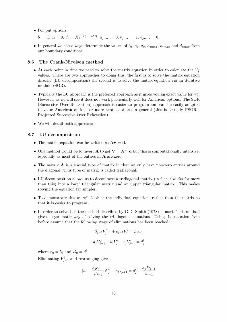
• For put options
b0 = 1, c0 = 0, d0 = Xe−r(T−i∆t), ajmax = 0, bjmax = 1, djmax = 0
• In general we can always determine the values of b0, c0, d0, ajmax, bjmax and djmax fromour boundary conditions.
8.6 The Crank-Nicolson method
• At each point in time we need to solve the matrix equation in order to calculate the V ij
values. There are two approaches to doing this, the first is to solve the matrix equationdirectly (LU decomposition) the second is to solve the matrix equation via an iterativemethod (SOR).
• Typically the LU approach is the preferred approach as it gives you an exact value for V ij .
However, as we will see it does not work particularly well for American options. The SOR(Successive Over Relaxation) approach is easier to program and can be easily adaptedto value American options or more exotic options in general (this is actually PSOR -Projected Successive Over Relaxation).
• We will detail both approaches.
8.7 LU decomposition
• The matrix equation can be written as AV = d.
• One method would be to invert A to get V = A−1d but this is computationally intensive,especially as most of the entries in A are zero.
• The matrix A is a special type of matrix in that we only have non-zero entries aroundthe diagonal. This type of matrix is called tridiagonal.
• LU decomposition allows us to decompose a tridiagonal matrix (in fact it works for morethan this) into a lower triangular matrix and an upper triangular matrix. This makessolving the equation far simpler.
• To demonstrate this we will look at the individual equations rather than the matrix sothat it is easier to program.
• In order to solve this the method described by G.D. Smith (1978) is used. This methodgives a systematic way of solving the tri-diagonal equations. Using the notation frombefore assume that the following stage of eliminations has been reached:
βj−1Vjj−1 + cj−1V
ij = Dj−1
ajVjj−1 + bjV
ij + cjV
ij+1 = dij
where β0 = b0 and D0 = di0.
Eliminating V ij−1 and rearranging gives
(bj −ajcj−1
βj−1)V i
j + cjVij+1 = dij −
ajDj−1
βj−1
48

which can be written in the form
βjVij + cjV
ij+1 = Dj
where βj = bj − ajcj−1
βj−1and Dj = dij −
ajDj−1
βj−1(1)
The last set of simultaneous equations are given by
βjmax−1Vijmax−1 + cjmax−1V
ijmax = Djmax−1
ajmaxVijmax−1 + bjmaxV
ijmax = dijmax
and by the same process as before elimination of the V ijmax−1 term yields
(bjmax −ajmaxcjmax−1
βjmax−1)V i
jmax = dijmax −ajmaxcjmax−1
βjmax−1
i.e.αjmaxV
ijmax = Djmax (2)
• The equations are now in the form where one can start obtaining results for the unknownV values. Using equations 1 and 2, the values for V are as follows:
V ijmax =
Djmax
βjmax
V ij =
1
αj(Dj − cjV
ij+1) (3)
where the βs and Djs are given by
α0 = b0; βj = bj −ajcj−1
βj−1(4)
D0 = di0; Dj = dij −aj
βj−1Dj−1, (5)
where j = 1, 2, 3, ...., jmax.
8.8 Comments
• So this method allows us to move from a known value of V ijmax up to V i
0 using the formulae
here. Thus we have an explicit algorithm for calculating V ij for all values of i and j that
does not involve the inversion of a large, sparse matrix.
• The method will be to start from expiry, then move back a time period, calculate thevalues of aj , bj, cj and dij (note that dIj uses V imax
j values) and use these together with
the equations in the previous subsection to calculate all of the values of V imax−1j and then
step back one more time step and repeat the process until we reach i = 0 when we havethe current option value.
• To calculate the V ij values, work up from j = 0 to obtain βj and Dj using equations (4)
and (5) and then work down from jmax to determine V ij using equation (3).
• This is not too difficult to program.
49

8.9 SOR method
• The SOR method is a simpler approach but can be slightly less accurate and take a littlelonger as it relies upon iteration.
• If we consider each of the individual equations from AV = d we have that
a1Vi0 + b1V
i1 + c1V
i2 = di1
a2Vi1 + b2V
i2 + c2V
i3 = di1
............ = ...
ajVij−1 + bjV
ij + cjV
ij+1 = dij
............ = ...
ajmax−1Vijmax−2 + bjmax−1V
ijmax−1 + cjmax−1V
ijmax = dijmax−1
• The Jacobi method says that we can trivially rearrange these equations to get:
V ij =
1
bj(dij − ajV
ij−1 − cjV
ij+1)
• The Jacobi method is an iterative one that relies upon the previous equation. Taking aninitial guess for V i
j , denoted as V i,0j (typically V i+1
j ) then we iterate using the formulabelow for the (k + 1)th iteration:
V i,k+1j =
1
bj(dij − ajV
i,kj−1 − cjV
i,kj+1)
this is performed until the difference between V i,kj and V i,k+1
j is sufficiently small for allj.
• A more effective process is the Gauss-Seidel method that uses the fact that when wecalculate V i,k+1
j we already know V i,k+1j−1 and so we use this information to write a new
iterative formula
V i,k+1j =
1
bj(dij − ajV
i,k+1j−1 − cjV
i,kj+1)
• The SOR method is another slight adjustment. It starts from the trivial observation that
V i,k+1j = V i,k
j + (V i,k+1j − V i,k
j )
and so (V i,k+1j −V i,k
j ) is a correction term. It may well be the case that the iterations con-
verge faster to the correct value if we over correct. This is true if V i,kj → V j
i monotonicallyin k. So the SOR algorithm says that
yi,k+1j =
1
bj(dij − ajV
i,k+1j−1 − cjV
i,kj+1)
V i,k+1j = V i,k
j + ω(yi,k+1j − V i,k
j )
where 1 < ω < 2 is called the over-relaxation parameter.
• This can be shown to converge for our values of a and c.
50

8.10 American options: Explicit
• As we well know the American option pricing problem requires us to calculate the optimalearly exercise strategy. To do this you typically compare the continuation value with theearly exercise value, if the latter is larger then you exercise.
• To value an American option using the explicit finite difference method is pretty straight-forward, you calculate the continuation value CoV i
j by the valuation formula below
CoV ij =
1
1 + r∆t(AV i+1
j+1 +BV i+1j + CV i+1
j−1 )
and then compare this to the early exercise payoff. Thus for a put:
V ij = max[X − j∆S,
1
1 + r∆t(AV i+1
j+1 +BV i+1j + CV i+1
j−1 )]
• This is similar to how we value American options using the binomial tree
American put option: Explicit
...0
∆S
2∆S
.
.
j∆S
.
.
SUImpose upper boundary at SU
Impose lower boundary at 0
terminal
boundary
0 T∆t 2∆t (i+1)∆t ...i∆t
Move through “interior” of
mesh/grid using this rule
8.11 American put option: C-N
• The American option pricing problem is slightly more complex for the Crank-Nicolsonmethod. To see this consider the process of calculating V i
j
• The value of the option V ij , for all values of j, depends also upon the value of V i
j−1 and V ij+1.
Thus, when we are determining where to early exercise we also need to simultaneouslyknow these values. However as we change one of these values then the other values willalso change.
• This means that it is not possible to simply compare the early exercise value to thecontinuation value as, if you decide to early exercise this will change all of the values ofV ij and then this decision may well have been suboptimal.
51

8.12 PSOR
• One, simple solution to this problem is to adapt our SOR method to PSOR (ProjectedSOR) which enables us to deal with early exercise constraints.
• The only difference between SOR and PSOR is that for each calculation in the iterationyou also check whether or not it would be optimal to exercise. Thus our previous iterationtechnique
yi,k+1j =
1
bj(dij − ajV
i,k+1j−1 − cjV
i,kj+1)
V i,k+1j = V i,k
j + ω(yi,k+1j − V i,k
j )
to (in the case of the American put option)
yi,k+1j =
1
bj(dij − ajV
i,k+1j−1 − cjV
i,kj+1)
V i,k+1j = max(V i,k
j + ω(yi,k+1j − V i,k
j ),X − j∆S)
8.13 Convergence and accuracy
• If the option price and the derivatives are well behaved then we know that the errorof the Explicit method should be O(∆t, (∆S)2) and the Crank-Nicolson method shouldbe O((∆t)2, (∆S)2). These can be considered similar to the distribution error for thebinomial tree as this will be the general convergence to the correct option value.
• If convergence is smooth like this then the results are also amenable to extrapolation.
• Unfortunately just as for binomial trees, finite-difference methods will also suffer fromnon-linearity error if the grid is not correctly aligned with respect to any discontinuitiesin the option value, or the derivatives of the option value.
8.14 Non-linearity error
• The nice thing about finite difference methods in general are that you have the freedomto construct the grid as desired and so it is quite simple to construct the grid so that youhave a grid point upon any discontinuities.
• For example, if we consider an European call or put option then the only source of non-linearity error is at S = X at expiry. Thus you should always choose ∆S so that X = j∆Sfor some integer value of j.
• So if in this case S0 = 100 and X = 95, you need a suitably large SU and a ∆S which isa divisor of 95. Thus if you want 5000 S steps then a reasonable choice for ∆S may be0.076, which give SU = 4× 95 = 380 and j = 1250 is the position of the exercise price.
8.15 Barrier options
• As we have seen when pricing barrier options with the binomial method, there is a largeamount of non-linearity error that comes from not having the nodes in the tree alignedwith the position of the barrier.
• Thus with barrier options we have two sources of non-linearity error, the error from thebarrier and the error from the discontinuous payoff.
52

• However, with the finite difference grid it is relatively easy to align the grid so that youhave nodes on the barrier and on the exercise price at expiry.
• For a down and out barrier option choose SL (the lower value of S) to be on the barrierand then, as in the previous example, choose ∆S so that the exercise price is also on anode.
• For example if B = 90 and X = 95 if you require 5000 steps, choose ∆S = 0.05, so thatSU = 340, and the barrier is at j = 0 and the exercise price is at j = 100.
8.16 Overview
• We have introduced the Crank-Nicolson finite difference method. This is slightly harderto program than the explicit method in that you have to solve a matrix equation at eachtime point but it has faster convergence and is stable.
• Applying the method to American options requires the use of PSOR which again is morecomplex than the method for valuing American options using the explicit method.
• Finally, we saw that with finite-difference methods as you can choose the dimensions ofthe grid so as to remove the nonlinearity error.
53

9 Finite differences: further considerations
• Here we will complete our look at finite-difference methods by looking at body-fitted co-ordinates, these allow us to fit the grid to avoid any non-linearity error even when thereis early exercise.
9.1 Body-fitted coordinates
• As discussed, the main problem when applying numerical schemes to problems involvingearly exercise is that the position of the early exercise boundary is not known a priori.This often means that when constructing a grid this boundary does not often fall on agrid point, or node, causing a degree of non-linearity error.
• The usual numerical schemes: lattice methods and basic finite difference schemes areunable to fix the grid correctly.
• The method described here involves keeping the time axis fixed but transforming the Sto an S axis that moves with the free boundary.
9.2 The American put option
• The American put option price, P (S, t) is described by the Black-Scholes equation for thefollowing boundary conditions:
P (S, T ) = max(X − S, 0)
P (S ≤ Sf (t), t) = X − S
P (S, t) → 0 as S → ∞
• where, as usual, Sf (t) is the position of the free boundary at time t. To incorporate thebody-fitted co-ordinate system simply introduce the transformation
S = S − Sf (t)
• and so the range of S is from 0 to ∞. This will also ensure that, at every timestep,the S-dimension of the grid will range from the exact position of the free-boundary to asufficiently large value of S.
• This removes the nonlinearity error present in the previous schemes. This desired effectdoes come at a cost though. As the position of the early exercise boundary is not knowna priori, then the position of all the S values are also not known at each point in time.
• It is, thus, necessary to perform a technique analogous to a multivalued Newton-Raphsoniteration. This is undertaken in combination with the usual Crank Nicolson scheme. Thefirst point to note is that the above transformation leads to a slight change in the governingequation, since
∂P
∂t→ ∂P
∂t+
∂P
∂S
∂S
∂t=
∂P
∂t− ∂P
∂S
dSf
dt
and so the Black-Scholes equation becomes:
12σ
2(S + Sf )2 ∂
2P
∂S2+ r(S + Sf )
∂P
∂S+
∂P
∂t− ∂P
∂S
dSf
dt− rP = 0
54

• Fortunately the option value, P and the position of the free boundary Sf (t = T ) are both
known at expiry (i.e. Sf = X and P = max(−S, 0)) and so to calculate the values atT −∆t we simply perform an iterative scheme using these values as a starting point.
P (m+1)(i∆S, j∆τ) = P (m)(i∆S, j∆τ) + δPi for 0 ≤ i ≤ n
• At a given timestep j∆τ , after m iterations write the values at the n distinct P values inthe finite difference scheme and the value of Sf as
S(m+1)f (j∆τ) = S
(m)f (j∆τ) + δSf
• The value of P(0)i (i∆S, j∆τ) and S
(0)f (j∆τ) are taken to be the converged values of
Pi(i∆S, (j + 1)∆τ) and Sf ((j + 1)∆τ) respectively. All that remains is to calculate thesuccessive values of the δPi’s and δSf . In order to do this a Crank-Nicolson scheme isused.
9.3 Crank-Nicolson
• The principal differences from the basic scheme are, first, that the unknown values arethe δPi’s and δSf . Secondly, there is also be an extra column in the matrix to cope withthe new extra unknown, δSf . There are, now, N +1 equations in N +2 unknowns, this is
easily overcome by using both the boundary conditions at S = 0 (S = Sf ) including thecondition from before and the smooth pasting condition
∂P
∂S= −1
• The next step requires arranging the difference equations into a system with the unknownvalues are on one side and the known ones on the other. The approximation for thederivatives is as usual. In general P (i∆S, j∆t) is denoted Pi,j and the resulting set ofequations, for 0 ≤ i ≤ N , is
aiδPi−1 + biδPi + ciδPi+1 + diδSf = ei
where, as before, the values of ai, bi, ci, di and ei need to be calculated.
9.4 Boundary conditions
• There are two boundary conditions at S = 0 and one at S = Smax. For these the valuesof a, b, c, d and e are known and are as follows:
– At S = 0:Pm0,j + δP0 = X − (S
(m)f,j + δSf )
and using a one-sided difference scheme we can generate an equation for the derivativecondition
−3P(m)0,j + 4P
(m)1,j − P
(m)2,j − 3δP0 + 4δP1 − δP2
2∆S= −1
55

which rearrange to give
δP0 + δSf = X − P(m)0,j − S
(m)f,j ,
3δP0 + 4δP1 − δP2 = −2∆S + 3P(m)0,j − 4P
(m)1,j + P
(m)2,j
and at Smax:δPN = −P
(m)N,j .
9.5 Method
• There are now a series of N + 2 equations in N + 2 unknowns which can be solved usinglinear algebra techniques. In matrix form the problem can be displayed as
1 0 0 . . . . . 1−3 4 −1 0 . . . . 0a1 b1 c1 0 . . . . d10 a2 b2 c2 . . . . d2. . . . . . . . .. . . . ai bi ci . di. . . . . . . . .0 . . . . . 0 bN 0
δP0
δP1
δP2
.
.δPN−1
δPN
δSf
=
X − P(m)0,j − S
(m)f,j
.e1....
−P(m)N,j
A reduction technique is then applied to solve the system. First, remove all the ci terms,starting from cN−1 by using
c′
i = ci − bi+1cibi+1
• and as a result the other terms are affected, namely
b′
i = bi − ai+1cibi+1
d′
i = di − di+1cibi+1
e′
i = ei − ei+1cibi+1
• There is a slight anomaly in the reduction technique in that the second row in the matrixhas an extra column. This is easily overcome as this last term is removed using b2 and theother terms adjusted accordingly and then the c0 term is removed by using c1 as before.
• The matrix is now in the form:
0 0 0 . . . . . d′
−1
b′
0 0 0 0 . . . . d′
0
a1 b1 0 0 . . . . d′
1
0 a′
2 b′
2 0 . . . . d′
2
. . . . . . . . .
. . . . a′
i b′
i 0 . d′
i
. . . . . . . . .
0 . . . . . 0 b′
N 0
δP0
δP1
δP2
.
.δPN−1
δPN
δSf
=
X − P(m)0,j − S
(m)f,j
.
e′
1
.
.
.
.
e′
N
56

• but from the top row it is possible to calculate the value of δSf as
δSf =e′
−1
d′
−1
and from the second row the value of δP0 can be deduced
δP0 =e′
0 − d′
0δSf
b′
0
• then continue this regime to calculate the values of δPi for 1 ≤ i ≤ N using
δPi =e′
i − d′
iδSf − a′
iδPi−1
b′
i
• This scheme is equivalent to a Newton-Raphson iteration and, as such, must have con-verged before moving forward to the next timestep.
• Depending on the accuracy required, we select a value for which all the δPi’s or δSf needto be less than to have assumed convergence - a typical value is 1 ∗ 10−8
9.6 Time adjustment
• In order to try and predict the movement of the early exercise boundary, a somewhatunrigorous scaling of the timesteps is carried out. It is known that the early exerciseboundary does not move exactly as
√τ (This is because there are also log-terms present
in the exact representation of the early exercise boundary as τ → 0.) However, it is a goodenough approximation to ensure that there are no stepsize constraints in the body-fittedCrank Nicolson scheme.
• This scaling is very easy to implement. Simply divide time into N steps of size ∆t = T/Nas usual, however when using ∆t in the numerical calculation instead use ∆t = T/N2
• Often, when using body-fitted co-ordinates, it can be difficult to correctly determine theposition of the boundary (in this case, near to τ = 0) but this ensures that the earlyexercise boundary follows, approximately, its proper form.
• Now that any nonlinearity error has been removed it would be expected that the conver-gence to the correct option price is at the rate O((∆t)2, (∆S)2). If so, it should be possibleto extrapolate results, assuming that there is also no non-linearity error occurring at thestrike price at maturity.
• At expiry the early exercise boundary is at the strike price and, thus, extrapolation canbe performed. As the results converge at the same rate in both the t and the S directionsit is possible to perform just one extrapolation.
57

10 Monte Carlo methods for American options the Longstaff
and Schwartz method
10.1 Overview
• We have looked at using Monte Carlo methods for most types of options, but they strugglewith early exercise
• This is the subject of lots of research at the moment and we have seen the basic idea ofsome of the methods.
• What we present here is one of the easiest methods to understand and implement.
• There are still issues with how it performs in practise which we will also deal with here.
• The key calculations when valuing an American option are determining the early exercisevalue and the expected continuation value.
• The option value at any point in time will be the larger of these two values.
• The early exercise value is simple to calculate at any point in time. The continuationvalue is typically determined by a backward iteration approach, where the value now isthe discounted expected option value at the next instance in time.
• The key information we need to know is given the share price at time t, what is theexpected option value at time t+∆t.
• This is simple to determine in binomial models but less so in Monte Carlo approaches.
10.2 The least squares method
• This is a technique for fitting a set of functions to (given) data.
• Here we describe the procedure for an mth degree polynomial - it is straightforward toextend the idea to a general class of polynomial
• When using an mth degree polynomial
y = a0 + a1x+ a2x2 + ...+ amxm
to approximate the given set of data, (x1, y1), (x2, y2), ..., (xn, yn), where n ≥ 3, the bestfitting curve f(x) has the least square error, i.e.,
Π =n∑
i=1
[yi − f(xi)]2 =
n∑
i=1
[yi − (a0 + a1xi + a2x2i + ...+ amxmi )]2 = min
• Note that a0, a1, a2, ..., and am are unknown coefficients while all xi and yi are given. Toobtain the least square error, the unknown coefficients a0, a1, a2, ..., and am must yield
58

zero first derivatives.
∂Π
∂a0= 2
n∑
i=1
[yi − (a0 + a1xi + a2x2i + ...+ amxmi )] = 0
∂Π
∂a1= 2
n∑
i=1
xi[yi − (a0 + a1xi + a2x2i + ...+ amxmi )] = 0
∂Π
∂a2= 2
n∑
i=1
x2i [yi − (a0 + a1xi + a2x2i + ...+ amxmi )] = 0
.............
∂Π
∂am= 2
n∑
i=1
xmi [yi − (a0 + a1xi + a2x2i + ...+ amxmi )] = 0
• Expanding the above equations, we have
n∑
i=1
yi = a0
n∑
i=1
1 + a1
n∑
i=1
xi + α2
n∑
i=1
x2i + . . .+ am
n∑
i=1
xmi
n∑
i=1
xiyi = a0
n∑
i=1
xi + a1
n∑
i=1
x2i + α2
n∑
i=1
x3i + . . .+ am
n∑
i=1
xm+1i
n∑
i=1
x2i yi = a0
n∑
i=1
x2i + a1
n∑
i=1
x3i + α2
n∑
i=1
x4i + . . . + am
n∑
i=1
xm+2i
................n∑
i=1
xmi yi = a0
n∑
i=1
xmi + a1
n∑
i=1
xm+1i + α2
n∑
i=1
xm+2i + . . .+ am
n∑
i=1
x2mi
• The unknown coefficients a0, a1, a2, ..., and am can hence be obtained by solving theabove linear equations.
• There are also many library routines avaliable to do the job.
10.3 Longstaff and Schwartz (2001)
• The Longstaff and Schwartz method, essentially estimates the conditional expected optionvalue at the next time step by simulating lots of paths and then carrying out a regressionof the future realised option value as a function of the current value of the underlyingasset.
• This gives an approximation for the continuation value that can then be compared to theearly exercise value and then we know the option value at each point in time on each path.
• In terms of Monte Carlo pricing, all we actually need to know is the rule for early exercising,so we know when we receive the cash flows and the value of the option is the average ofthe discounted payoffs for each path.
• We will explain the method via an example and then describe the general method.
59

10.4 Example
• We will attempt to value a Bermudan put option where exercise is possible now and atthree future dates. S0 = 1, X = 1.1, r = 0.06.
• The first step is to simulate some paths, the table below denotes the results:
Stock price paths
Path t = 0 t = 1 t = 2 t = 31 1.00 1.09 1.08 1.342 1.00 1.16 1.26 1.543 1.00 1.22 1.07 1.034 1.00 .93 .97 .925 1.00 1.11 1.56 1.526 1.00 .76 .77 .907 1.00 .92 .84 1.018 1.00 .88 1.22 1.34
• We need to use this information to determine the continuation value at each point in timefor each path. To do this we will construct a ”Cash Flow Matrix” at each point in time.
Continuation value at t = 2
• The table below denotes the cash flows at t = 3 assuming that we held the option thatfar:
Cash-flow matrix at t = 3
Path t = 1 t = 2 t = 31 – – .002 – – .003 – – .074 – – .185 – – .006 – – .207 – – .098 – – .00
• The next step is to attempt to find a function that describes the continuation value attime 2 as a function of the value of S at time 2.
• To do this we use a regression technique, that takes the values at time 2 as the ”x” valuesand the discounted payoff at time 3 as the ”y” values.
Continuation value at t = 2
60
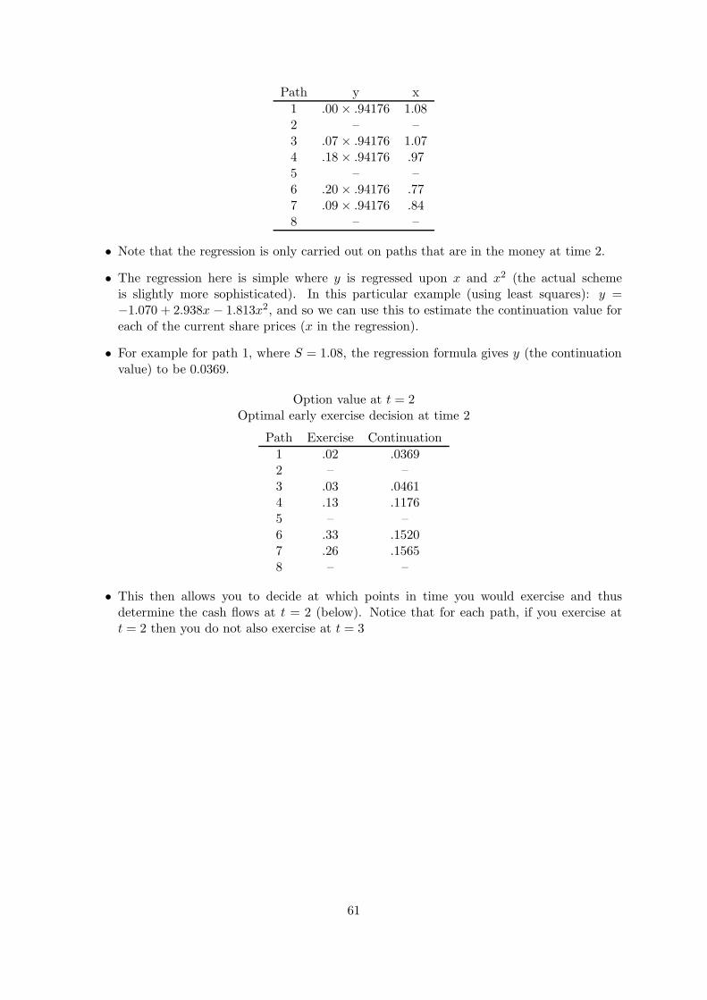
Path y x
1 .00× .94176 1.082 – –3 .07× .94176 1.074 .18× .94176 .975 – –6 .20× .94176 .777 .09× .94176 .848 – –
• Note that the regression is only carried out on paths that are in the money at time 2.
• The regression here is simple where y is regressed upon x and x2 (the actual schemeis slightly more sophisticated). In this particular example (using least squares): y =−1.070 + 2.938x − 1.813x2, and so we can use this to estimate the continuation value foreach of the current share prices (x in the regression).
• For example for path 1, where S = 1.08, the regression formula gives y (the continuationvalue) to be 0.0369.
Option value at t = 2Optimal early exercise decision at time 2
Path Exercise Continuation
1 .02 .03692 – –3 .03 .04614 .13 .11765 – –6 .33 .15207 .26 .15658 – –
• This then allows you to decide at which points in time you would exercise and thusdetermine the cash flows at t = 2 (below). Notice that for each path, if you exercise att = 2 then you do not also exercise at t = 3
61

Cash-flow matrix at time 2Path t = 1 t = 2 t = 31 – .00 .002 – .00 .003 – .00 .074 – .13 .005 – .00 .006 – .33 .007 – .26 .008 – .00 .00
Continuation value at t = 1
• We can apply the same process to t = 1, for each of the paths that are in the money weregress the discounted future cash flows (y) on the current value of the underlying asset(x), where x and y are as given below:
Regression at time 1Path y x
1 .00× .94176 1.092 – –3 – –4 .13× .94176 .935 – –6 .33× .94176 .767 .26× .94176 .928 .00× .94176 .88
• The regression equation here is y = 2.038 − 3.335x + 1.356x2 and again we use this toestimate the continuation value and decide on an early exercise strategy.
• The next table compares the two values and the final table denotes the early exercise orstopping rule.
Optimal early exercise decision at time 1Path Exercise Continuation
1 .01 .01392 – –3 – –4 .17 .10925 – –6 .34 .28667 .18 .11758 .22 .1533
• The early exercise strategy is as follows:
Stopping rule
62

Path t = 1 t = 2 t = 3
1 0 0 02 0 0 03 0 0 14 1 0 05 0 0 06 1 0 07 1 0 08 1 0 0
• From this we can then value the option, by forming the final cash flow matrix from thisrule.
Option cash flow matrixPath t = 1 t = 2 t = 31 .00 .00 .002 .00 .00 .003 .00 .00 .074 .17 .00 .005 .00 .00 .006 .34 .00 .007 .18 .00 .008 .22 .00 .00
• So the option value is the average of the discounted cash flows, so in this case:
V0 =18(0 + 0 + 0.07e−3r + 0.127e−r + 0.34e−r + 0.18e−r + 0.22e−r) = 0.1144
10.5 More sophisticated regression
• In general the regression here y = a1+a2x+a3x2 is not going to be satisfactory, especially
as we will have far more than 8 paths when attempting to find the functional form of thecontinuation values.
• In fact the general form of y is:
y =M∑
j=0
ajFj(x)
• The user decides upon M the number and the functional form Fj(x) (in our exampleFj(x) = xj) where Fj(x) is called a basis function.
• Although Longstaff and Schwartz suggest Laguerre polynomials provide the best fit, myfavourite is Chebyshev polynomials. However, you are free to choice whichever basisfunctions you want (e.g. Polynomial as in the example, Chebyshev, Hermite, Laguerre,etc.)
• The Laguerre polynomials are given by:
F0(x) = exp(−x/2)
F1(x) = (1− x)exp(−x/2)
Fn(x) = exp(−x/2)ex
n
dn
dxn(xne−x)
63

• Chebyshev polynomials are given by:
Fn(x) = cos(n(cos−1 x))
In particular T0(x) = 1, T1(x) = 1, T2(x) = 2x2 − 1, .....
• Then the least squares approach approximates the constants aj , and when we have thesevalues we can use them to predict the continuation value for each value of S at every pointin time.
10.6 Longstaff and Schwartz - general procedure
• Decide on the number of sample paths N , the number of basis functions for the regression,M , and the type of basis functions Fj(x) and the number of observation dates d.
• Draw Nd Normally distributed random numbers and simulate the sample paths for theunderlying asset at each point in time Sn
ti 1 ≤ i ≤ d, 1 ≤ n ≤ N
• At expiry t = td, record the cash flow values CFn(td) which for a put are max(X −Sntd, 0)
• Move back to t = td−1 for each path where Sntd−1
< X calculate the continuation value as
CV n(td−1) = e−r(td−td−1)CFn(td). From these values perform the regression to determinethe functional form of the continuation value, y(S) where S is the value of the underlyingasset
• Recalculate the continuation value as CV n(td−1) = y(Sntd−1)
• For every path calculate the cash flow value where if the continuation value CV n(td−1) <X − Sn
td−1then CFn(td−1) = X − Sn
td−1and CFn(ti) = 0 for i > d − 1 otherwise
CFn(td− 1) = 0
• Repeat this process for the previous time step until you have CFn(ti) for all i and n. Notethat in general to calculate CV n(ti) before the regression
CV n(ti) =d
∑
n=i+1
e−r(tn−ti)CFn(tn)
• The option value V0 is then
V0 =1
N
N∑
i=1
M∑
j=1
e−rtjCF i(tj)
• When you have more than one underlying asset in order to perform the regression youneed to have basis functions in all of the underlying assets as well as in the cross termsbetween them (i.e. in S1, S2 and S1S2).
• This means that the number of basis functions will increase exponentially as you increasethe number of underlying assets, although it is not necessary in practise to have too largea number of basis functions.
64

10.7 How well does it perform?
• Longstaff and Schwartz provide proofs that as M → ∞ and N → ∞ the option valueobtained from their scheme converges to the theoretical value.
• This isn’t much use for practical considerations as you will be limited by how many basisfunctions you can calculate and how many simulations you can perform.
• There have been a few investigations into the method and the view of the method’sperformance are mixed: Broadie and Detemple (2004) say regression methods ‘often incurunknown approximation errors and are limited by a lack of error bounds’.
• A detailed appraisal of this technique by Moreno and Navas (2003) investigates the useof various polynomial fits and numbers of basis functions.
• It is not clear that increasing the number of basis functions actually increases the accuracyof the method and there is no real difference from using different types of basis functions(e.g. Chebyshev rather than Laguerre)
• For more complicated derivative pricing problems the trend is even less clear, sometimeserrors can increase as you add more basis functions (too many essentially fits the stochasticvalues of S exactly)
• In general, the method will provide good estimates but will be difficult to assess exactlyhow accurate it is.
• See Duck et al (2005) for some improvements on the basic Longstaff and Schwartz scheme(the latter provides superoptimal estimates, but these can be exploited using extrapola-tion).
10.8 Overview
• We have introduced a method for valuing options with early exercise features using sim-ulation.
• The main idea is to estimate the continuation value (as a function of the current underlyingasset price) by performing a least squares regression.
• The method converges to the correct option price but research shows that it is unclearhow well the method performs and how to estimate the error when using a finite numberof paths/ basis functions.
65

11 The QUAD method
In this chapter we consider a simple, widely applicable numerical approach for option pricingbased on quadrature methods. Though in some ways similar to lattice or finite-differenceschemes, it possesses exceptional accuracy and speed. Discretely monitored options are valuedwith only one time step between observations, and nodes can be perfectly placed in relationto discontinuities. Convergence is improved greatly; in the extrapolated scheme, a doubling ofpoints can reduce error by a factor of two-hundred and fifty-six. Complex problems (e.g fixed-strike lookback discrete barrier options) can be evaluated accurately and orders of magnitudefaster than by existing methods.
11.1 Introduction
With QUAD, a full range of final positions can be evaluated using just one time-step and theimprovement in efficiency is quite remarkable. For example, using a lattice method a doubling ofaccuracy requires approximately four times the computational effort, whereas using QUAD withSimpson’s rule implementation (see later), a four-fold increase in computational time improvesaccuracy by a factor of sixteen rising to a factor of two-hundred and fifty-six with extrapolation.
With QUAD, nodes can be positioned exactly as required, thus avoiding all non-linearityerror, even when pricing such exotic products as moving discrete barrier options and lookbackoptions with barriers. A welcome consequence of this eradication of non-linearity error is thatextrapolation can be used to reduce distribution error even further.
QUAD can be seen as analogous to a multinomial lattice in that the option prices arecalculated from values at nodes later in time, working backwards from maturity. However, italso has the added flexibility that nodes can be placed wherever desired and only one time stepis required between observations of exotic features. In many ways, it could be considered ‘theperfect tree’ method.
Figure 1 shows schematically how QUAD evaluates a down-and-out moving discrete barriercall option; a much more detailed summary of the method follows later. This option has a pay-off at maturity identical to a vanilla-call option, but this pay-off is contingent on the underlyingasset remaining above the level Bm at times Tm. If at these observation times the underlyingis below the barrier level then the option is ‘knocked out’ and becomes worthless.
Between barriers, the option value behaves precisely as a vanilla European option, and as aconsequence the well-known exact solution for such options can be employed to relate values,backwards in time, between successive barriers. It is only necessary to calculate option valueswhen the special feature, the knock out, applies. In contrast with lattice and finite-differencemethods there is no need to consider intermediate timesteps and it is possible to move to anyvalue of the underlying at each time-step. The nodes at each significant time-step may besimply positioned so as to cope with non-linearity, in this case the barriers and the strike priceat maturity.
It is well known that the majority of options can be written as either a finite or an infiniteset of nested (multiple) integrals.
11.2 Building blocks of the QUAD method
11.2.1 Adapting the Black-Scholes equation
As a starting point, consider the well-known Black and Scholes (1973) partial differentialequation for an option with an underlying asset following geometric Brownian motion:
∂V
∂t+
1
2σ2S2∂
2V
∂S2+ (r −Dc)S
∂V
∂S− rV = 0, (1)
66

Figure 1: A schematic diagram demonstrating the evaluation of a discrete moving barrier optionwith barriers at B1, B2 and B3, strike price X, time to maturity T4 and current underlyingprice of S. QUAD integrates across a set of points at each observation time (reduced in numberand shown in bold for only one point in each set before maturity
67

where V (S, t) is the price of the derivative product, S the current value of the underlying asset,t is time, T is the time to maturity r the risk-free interest rate, σ the volatility of the underlyingasset and X is the exercise price of the option. Dc is a continuous dividend yield which could,for example, be the foreign interest rate in a foreign exchange option.
Next make the following standard transformations in Eq. 1
x = log(St/X), (2)
y = log(St+∆t/X). (3)
It is important to note in what follows that ∆t is not restricted to small time periods. Thefinal conditions for a European option expiring at time T = t + ∆t with V (y, t + ∆t) aretransformed in straightforward fashion; e.g. the payoff for a call option max(St+∆t − X, 0)becomes max(Xey −X, 0). The value of the option at time t on an underlying asset St has anexact solution given by
V (x, t) = A(x)
∫ ∞
−∞B(x, y)V (y, t+∆t) dy, (4)
where,
A(x) =1√
2σ2π∆te−
12kx− 1
8σ2k2∆t−r∆t, (5)
and
B(x, y) = e−(x−y)2
2σ2∆t+ 1
2ky (6)
and
k =2(r −Dc)
σ2− 1. (7)
Also, let x0 be the x corresponding to the value of S at the outset, st i.e.
x0 = log(St/X). (8)
Henceforth the integrand here will be denoted as f(x, y), so that Eq. (4) becomes
V (x, t) = A(x)
∫ ∞
−∞f(x, y)dy (9)
where the integrand is given by
f(x, y) = B(x, y)V (y, t+∆t). (10)
The solution (4) contains an integral which, in general, cannot be evaluated analytically interms of simple functions, although for European options it is easily converted to the proba-bility density function for the Normal distribution. For more complicated options, numericaltechniques are required to evaluate the integral in Eq. (4). The intuition behind QUAD is thatalthough Eq. (4) is not valid across all points in time for anything other than a plain Europeanoption, the valuation problem can be sliced into consecutive time intervals, during which Eq.(4) is locally applicable. Imposition of the appropriate option features at their corresponding’observation’ times provides a link between these consecutive intervals, and solution of complexproblems becomes possible.
68

11.3 Quadrature methods
There are many different methods of numerical integral evaluation. Simpson’s rule is usedas a starting point because it is robust, simple, nimble, well-known and has fast convergence:of order (δy)4, where δy is the size of the gap between points (or of order N−4 where N is thenumber of steps). By comparison a trinomial tree converges merely with N−1 or in some cases
only with N− 12 . Even the more sophisticated finite difference methods at best converge at the
rate of (∆S2,∆t2) where ∆S and ∆t are the step sizes in the S and t directions respectively. Useof the trapezoidal rule will also be discussed here, although virtually any quadrature method isapplicable, including higher-order schemes and Gaussian quadrature.
11.3.1 Simpson’s rule
Although Simpson’s rule was devised as long ago as 1743, it remains one of the most accu-rate and popular methods for approximating integrals. The idea is conceptually simple: for afunction of y, f(y), plotted against y divide the desired range, [a1, a2] into intervals of a fixedlength and then approximate the area under the curve by summing the area of the individualregions. This yields the following expression, for a step size of δy,
∫ a2
a1
f(y) dy ≈ δy
6{f(a1) + 4f(a1 +
1
2δy) + 2f(a1 + δy) + 4f(a1 +
3
2δy)
+ 2f(a1 + 2δy) + · · ·+ 2f(a2 − δy) + 4f(a2 −1
2δy) + f(a2)}. (11)
It is straightforward to show that for smooth functions the error term associated with thismethod decreases at a rate of order (δy)4, i.e. a doubling of the number of steps reduces theerror by a factor of sixteen.
11.3.2 Trapezoidal rule
The trapezoidal rule is an even simpler quadrature method but is slower to converge, ata rate of (δy)2. It is included here because the procedure can save computational time whenpricing options for which the overall valuation technique puts other, more stringent, limitationson convergence, thus making the use of more accurate quadrature schemes superfluous.
∫ a2
a1
f(y) dy ≈ δy
2{f(a1) + 2f(a1 + δy) + 2f(a1 + 2δy) · · · + 2f(a2 − δy) + f(a2)}. (12)
The trapezoidal rule will find a reasonably accurate value more quickly than will Simpson’s ruleand so when speed is required rather than accuracy, the trapezoidal rule is sometimes moreappropriate.
11.4 Method and general application
In order to demonstrate how the quadrature component is incorporated into the QUADmethod, this section first considers the simple case of a vanilla call option. Here there is onlyone observation time, at maturity, and calculations are complete in a single time step. The closedform solution for this option is then used to verify the accuracy of the quadrature scheme. Moreinteresting, challenging and complex problems will follow later.
69

11.4.1 Illustration using vanilla calls
In the case of a vanilla call valued now, time t, the payoff at maturity time, t + ∆t, ismax(St+∆t −X, 0). The integrand, Eq. (10) becomes
f(x, y) = B(x, y)×Xmax(ey − 1, 0). (13)
A numerical scheme is then implemented to evaluate the integral in Eq. (9) using Simpson’sRule, Eq. (11)
Simpson’s rule converges with (δy)4 but only when evaluating functions with continuousderivatives. The first derivative of the payoff to a call option is clearly discontinuous at thestrike price (since for S < X, ∂V∂S = 0, for S > X, ∂V∂S = 1). In order remove this ‘non-linearityerror’ and to conserve the overall accuracy of the quadrature scheme it is necessary to split theintegral into two parts, with the boundary precisely at S = X (or y = 0). The payoff functionin the range −∞ < S < X is continuous, as is the function in the range X < S < ∞. Infact, for a call option, since the value at maturity in the range −∞ < S ≤ X is equal to zero,there is no contribution to the integral from this range (correspondingly, for a put there is nocontribution from X ≤ S < ∞). The range of integration in y in Eq. (9) is doubly infinite andso this must be truncated; however for |y| ≫ |x|, the B(x, y) term in Eq. (4) will tend to zerovery quickly, and consequently leads to insignificant contribution to the overall integral outsidea computationally quite modest range of y. Practically, a range corresponding to asset pricemovements, up or down, within ten standard deviations during a time step proved more thanadequate.
To value the call option at time t with asset price St, the method is as follows (see alsofigure 2). The value of y at the discontinuity (here, the strike price) is defined to be b, whichin the case of a vanilla option is clearly zero. The truncated range of integration is taken tobe [ymin, ymax] , and the integers N+ and N− are the number of steps taken in the half ranges[b, ymax] and [ymin, b] respectively. Since the value of the function below b for a vanilla call optionis zero, this region does not contribute to the option valuation. For a call option, then,
N+ =
[
ymax − b
δy
]
and N− = 0, (14)
where [a] denotes the integer closest to a and δy is the step size in y. An implementation ofSimpson’s rule would have the steps, i, say, with 0 ≤ i ≤ N+ with y = b + iδy and use valuesat these points and half way in between.
Using these new limits along with Eq. (4) the expression for the option price V (x, t) is
V (x, t) ≈ A(x)
∫ N+δy
0f(x, y) dy (15)
which, on implementing Simpson’s rule, Eq. (11), is
≈ A(x)δy
6
(
f(x, 0) + 4f(x,1
2δy) +
(N+−1∑
i=1
2f(x, iδy) + 4f(x, (i +1
2)δy)
)
+ f(x,N+δy)
)
(16)
and, by the definition of f(x, y) in Eqs. (9) and (13), this is
≈ A(x)δy
6
(
B(x, 0)V (0, t +∆t) + 4B(x,1
2δy)V (
1
2δy, t+∆t) + . . .
+B(x,N+δy)V (N+δy, t+∆t)
)
. (17)
70

Figure 2: A demonstration of QUAD used to evaluate a European call option (V (St, t)). y isthe transformed value of the underlying, S, δy is the step size, X is the strike price, ∆t is thetime to maturity and functions A(x) and B(x, y) are as described in Eqs. 5 and 6 respectively.
This calculation is no more complicated than calculating the option value using a latticemethod, however in QUAD the contribution at the previous timestep comes from many nodesrepresenting different levels of the underlying asset not just two or three.
Figure 2 depicts the valuation process. A range of y values at maturity is chosen, increasingin steps of δy from y = 0 (the discontinuity) where the asset price, S, is equal to the exerciseprice, X see Eq. (3). The option value at time t is then found by integrating Eq. (4) usingSimpson’s rule via Eq. (17). Since a plain European call is being used as a simple example,valuation is achieved in a single time step and, in this case, is directly comparable with valuationusing the known analytical solution commonly available in finance texts, such as Hull (2000).
The valuation can be quickly repeated for other possible current asset prices (transformedas x in Eq. (2)). In more complex option valuations these values one step back in timefrom maturity to another discontinuity become, in their turn, the basis for further integrationbackwards in time. This is reminiscent of backward valuation using a tree or finite differencelattice but with the important difference that large time steps are used, set by the periodbetween discontinuities.
Table I shows the results of applying this method to the pricing of a European call optionusing Simpson’s rule. To reduce the distribution error still further, a simple Richardson-typeextrapolation procedure was adopted. This was undertaken by performing calculations withtwo stepsizes δy1 and δy2, producing option values V1 and V2, respectively. An improved valueVext may be obtained through extrapolation, viz.
Vext =(δy1)
dV2 − (δy2)dV1
(δy1)d − (δy2)d, (18)
71

where (δy)d is the rate at which the error decreases for the unextrapolated data. Assuming thatthe position of the discontinuity has been accurately gauged, then for Simpson’s rule d = 4.
Absolute RMS errors have been calculated using sixteen different options, both with andwithout the extrapolation described by Eq. (18) (denoted by QUAD and QUADext respectively).Results are benchmarked against those from a trinomial method (denoted by TRIN). Timingswere obtained using a Pentium III 550 MHz computer and the NAG Fortran 95 v4.0 optimizedcompiler, and indicate excellent performance of the present scheme when compared with thestandard trinomial tree method. However, a more demanding test of the scheme is its applicationto more complex options for which no analytic, closed form solutions are known; these areconsidered next.
ABSOLUTE ROOT MEAN SQUARED ERRORS
N TRIN K QUADext QUAD(time/seconds) (time/seconds) (time/seconds)
European call options:
100 0.013879152 10 0.000008539 0.000246595(0.00) (0.00) (0.00)
200 0.010018265 20 0.000000087 0.000015034(0.01) (0.00) (0.00)
500 0.001833449 30 0.000000007 0.000002956(0.03) (0.00) (0.00)
1000 0.000600399 40 0.000000001 0.000000934(0.14) (0.00) (0.00)
2000 0.000405737 50 0.000000000 0.000000382(0.56) (0.00) (0.00)
Table I: Parameters are as follows: S = 100,X = 95/105, σ = 0.2/0.4,r = 0.06/0.2,∆t = 0.5/1,Dc = 0. TRIN is the basic trinomial modeldescribed in Hull (2000) with N steps in the lattice. QUAD,QUADext are results using Simpson’s rule, the latter extrapolated.
K is such that δy =√∆t/K.
11.5 Application to multiply-observed options
A discrete path-dependent option is one where the price of the underlying asset beforematurity is important only at discrete points in time, referred to here as observation times.The valuation of the option in between these times is described by the Black-Scholes partialdifferential equation Eq. (1).
Consider a path-dependent option observed M times during its lifetime. Conceptually thisis divided for valuation purposes into M separate options. These options, denoted Vm, havematurities Tm where m = 1, 2, . . . ,M . Let ∆tm be equal to Tm−Tm−1. Given the current time,t, the maturity of the complete option is at time TM given by
TM = t+
M∑
m=1
∆tm. (19)
Moving backwards from this maturity, whenever an observation time is encountered , Eq.(4), is evaluated for the period between that time and the next observation later in time. Forexample, with a Bermudan option the process could begin with integration of Eq. (4) coveringthe time period from the final possibility of early exercise until the maturity of the option.
72

At each observation time Tm the option is priced for a full range of x. These x values thenbecome the y values used in the integration to find the x values at the previous time step, Tm−1
and so on until the complete option is valued. The values of ymax and ymin for a truncated rangeof integration will change at each Tm and as a consequence will be denoted by ymaxm and yminm
respectively. The corresponding integer values of N+ and N− for the steps in the integrationwill be termed N+
m and N−m respectively.
The probability of an asset following geometric Brownian motion moving more than 10standard deviations within a time period is so small as to be insignificant. For this reason,curtailment of the range is possible such that, if T = Tm − t is the time before maturity, thenit is suggested that ymaxm = x0 + q and yminm = x0 − q are sufficient where
q = 10σ√T . (20)
This assumes that (r − Dc) is not unrealistically large, although adjustment for such valueswould be routine. For the same reason, it is not actually necessary to integrate over the entirerange of y for each value of x at every time step, but instead, letting
q∗ = 10σ√
∆tm, (21)
the integral for each individual x only needs to extend over the range [x− q∗, x+ q∗]. A point ofdiscontinuity in Vm will be denoted by bm. If the integer values of i at time Tm correspondingto this range are i+ and i−, where
i+ =
[
x− bm + q∗
δy
]
, (22)
and
i− =
[
x− bm − q∗
δy
]
, (23)
then Simpson’s rule should be employed for i between max(i−, N−) and min(i+, N+). If theδy chosen is too large, then results will clearly be inaccurate; fortuitously, it is generally very
obvious when this is the case. As a rough guideline, δy should always be smaller than√∆tm4 .
The location of discontinuities in the payoff function will be known a priori for some classesof options. For example, for a vanilla call or put option with exercise price, X, a discontinuityoccurs at y = 0; for a discrete barrier option, with a barrier position Bm at time Tm, a discon-tinuity occurs where y = log(Bm
X ). For other classes of option the position of the discontinuitymust be calculated at every observation time. For a Bermudan put option, for example, thelocation of the discontinuity, bm, at time Tm is where X − S = Pm+1(bm, Tm). Taking thisclass of option as a prototype, the location is determined as follows. It is convenient to definea function, g(x) say, which is zero at the desired value of x, bm. For a Bermudan put is
g(x) = X(1− ex)− Pm(x, Tm). (24)
The equation g(bm) = 0 may then be solved using Newton-Raphson iteration, which is gener-ally very quick to converge (rarely are more than ten iterations necessary to obtain machineprecision). In brief, initial values for bm and ∆bm are guessed (e.g 0 and −0.01, respectively)and a new value for bm is then:
b∗m = bm +∆bm. (25)
g(bm) and g(b∗m) must then be calculated, using Simpson’s rule for example, and then a new∆bm is given by
∆b∗m =−∆bmg(b∗m)
g(b∗m)− g(bm). (26)
73

Figure 3: A diagram depicting how QUAD is used to evaluate a discrete down and out calloption with barrier at S = B1 at time T1. x and y are the transformed values of the underlyingS, b1 is the transformed value of B1, δy is the step size, the time to maturity is T2. The optionvalue at T0 is calculated using an implementation of Simpson’s rule on the V1(y ≥ b1, T1) values.
The iterative process is repeated until g(bm) is sufficiently small, with the programming caveatthat iterations cease if the discontinuity is out of the range of integration, [yminm , ymaxm ] andhence, cannot be found.
Working back through time, from known final conditions, the first individual option VM (x, TM−1)can be priced for the entire range of underlying prices, in the manner described previously.The condition at the observation time (e.g. an early exercise condition) is imposed on thesevalues and then these adjusted values provide the new final conditions for the next option,VM−1(y, TM−1). The next option is priced using these final conditions and the process is re-peated until the value is found for V1(x, T0). Values for Vm(xi, Tm−1) must be calculated for allvalues of xi, where
xi = bm + iδy, (27)
and also, in the case of Simpson’s rule, at the points half way between. The i will run from N−m
to N+m, with one of these sometimes equal to zero (as in figure 2, for a European vanilla call
option). For the final option, V1, if the option value is just required at a single asset value, itis only necessary to calculate the value of V corresponding to St, i.e. x = log(St/X). Figure 3shows how QUAD is used to price a discrete down-and-out call option with one barrier, B1 atT1.
74

11.5.1 High frequency observations and continuous American features
Extrapolation is not only useful in removing ‘distribution error’ caused by the finiteness ofthe quadrature stepsize δy (using Eq. (18)) but can also be used to value options with moreobservations, or even with continuous, American style exercise. For continuous observation, theformula Eq. (18) may be utilized, but with δy replaced by T/M , where M is the number ofobservations. Although QUAD is tailored to be exceptionally powerful in valuing options withdiscrete observations, for those with continuous observation, its performance is at least compa-rable to all standard techniques, and, if the option is a particularly complex one with Americanfeatures, then QUAD may prove very useful. To value options with many observations, wherecomputing time is an issue (for example, three-dimensional lookbacks), extrapolation to manymultiple observations (taken at moments equally distributed in time) can be performed using:
VM3 =Md
1 (Md2 −Md
3 )VM1 +Md2 (M
d3 −Md
1 )VM2
Md3 (M
d2 −Md
1 ), (28)
where M1, M2 < M3 are the number of observations and VM is the respective option value.Note that there are certain cases (e.g. random moving barriers) where such extrapolation isnot applicable. A value of d of either 1
2 or 1 should be used depending on the particularproblem. Discretely monitored American put options (Bermudans), for example, converge tothe continuous solution at the rate of 1
M , where M is the number of observations, hence d =1; discrete barrier options converge with 1√
Mand so d = 1
2 . For a given type option it is
straightforward to gauge the appropriate value for d simply by running a few trial calculations.
11.6 Bermudan put options
A Bermudan put option is one which has an early exercise feature, similar to an Americanput, but only at certain prescribed dates. For a Bermudan put option the value of Pm (replacingV by P for a put option) at time Tm is
max(Pm+1(y = x, Tm),X − S), (29)
where PM+1 = max(X − S, 0).There will be a discontinuity in the second derivative of the option at the point where
Pm+1(Tm) is equal to (X − S). Above this point the value of the option is given by Pm+1(Tm), below it is equal to (X − S). Therefore the integration is split into two components to avoidany non-linearity error.
For the first option period evaluated, bM is the point where X = S, and so bM = 0. PM+1
above this point is equal to zero. Newton-Raphson may be used to find subsequent values ofbm, as described in Section 3.2.
Above bm, the value of Pm(y ≥ bm, Tm) is Pm+1(y = x, Tm), below the boundary the valueis simply the payoff, namely X − S, and so Pm(y ≤ bm, Tm) = X(1 − ey) . It is possible tocontinue using quadrature as before using Eq. (4)
Pm(x, Tm−1) ≈ A(x)
∫ ymaxm
bm
B(x, y)Pm(y ≥ bm, Tm) dy
+A(x)
∫ bm
yminm
B(x, y)×X(1 − ey) dy = I1 + I2. (30)
However I2 has a simple analytic form, related to the Black-Scholes solution for a put optionwithin the bound (−∞, bm]. In this region, in order to save computational time, the procedure
75

is then to use this analytic (Black-Scholes) form for I2(x), namely
I2(x) = Xe−r∆tmN(−d2)−Xex−Dc∆tmN(−d1), (31)
where N(.) is the cumulative probability distribution for a function that is normally distributedwith a mean of zero and standard deviation of 1, and d1 and d2 are given by:
d1 =x− bm + (r −Dc +
σ2
2 )(∆tm)
σ√∆tm
,
d2 = d1 − σ√
∆tm. (32)
11.7 Results
The accuracy and efficiency of QUAD are now compared with more familiar numericaltechniques for valuing the different types of options, described in the previous section. Table2 shows absolute root mean squared errors for a set of sixteen options. Results (QUAD) weregenerally extrapolated once (labelled QUADext) using Eq. (18) to further enhance accuracy. Inthe case of calculations performed using trapezoidal quadrature (in particular lookback optionsin three dimensions), extrapolation using Eq. (18) was carried out twice (QUADext2), first withd = 2, and then the resulting values (which may be regarded as having an error of O((δy)4))were the subject of a further application of Eq. (18) with d = 4. Choosing δy =
√∆tm/K,
extrapolation was performed with values obtained from K and K − 2, except in the case oflookback puts where K and K − 1 were used. For the lookback call options it was performedtwice using K,K − 1, and K − 2. Also, Dc is considered to be 0 for all options valued here.
For multiple compounds, Bermudan put, moving barrier, and American call options, theresults of the present method are compared with the basic trinomial model (Hull, 2000) denotedby TRIN. When valuing stationary discrete barrier options Ritchken’s (1995) approach (TRIN)is used but adapted, as suggested by Cheuk and Vorst (1996) in a straightforward mannerto treat discrete rather than continuous barriers. To value lookback options with a similarityreduction, Cheuk and Vorst’s (1997) two-dimensional binomial method (BINC), incorporatingthe placing of extra time steps between observations, (and adapted for AM different from St) isused for comparison. Finally, for the barrier lookback option, the benchmark is a basic three-dimensional trinomial model adapted for multiple steps between observations (TRIN3). Foreach case the exact solutions were obtained by using the current scheme when the δy was smallenough for the price to have converged to the given degree of accuracy (∼ 1 × 10⁻¹⁰). As anindication of the efficiency of the QUAD, average computational times are also displayed. Asbefore, timings were taken on a Pentium III 550 MHz system, using the NAG Fortran 95 v4.0compiler with optimization.
Although the basic trinomial tree approach was used as a benchmark for moving barrieroptions, improved results can be obtained using the AMM method of Ahn, Figlewski, and Gao(1999), though at a cost of considerably more complex programming. For comparison, AMM8with eighty time steps between observations gives absolute RMS of 0.00034 and takes an averagetime of 8.65 seconds whereas QUADext achieves better accuracy in a mere 0.28 of a second.
The results are shown in Table 2 and are excellent; for the two-dimensional models resultsin a given time are consistently orders of magnitude better than the benchmarks for all optionsconsidered. In the case of fixed-strike lookback discrete barrier options penny accuracy isachieved in 1.16 seconds whereas the trinomial method is, on average, 40 cents out after 23minutes. The superiority of QUAD over present methods is clear.
76
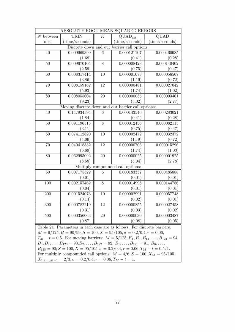
ABSOLUTE ROOT MEAN SQUARED ERRORS
N between TRIN K QUADext QUADobs. (time/seconds) (time/seconds) (time/seconds)
Discrete down and out barrier call options:
40 0.009969399 6 0.000121107 0.000460985(1.68) (0.41) (0.28)
50 0.009670104 8 0.000008423 0.000140402(2.59) (0.75) (0.47)
60 0.008317414 10 0.000001673 0.000056567(3.86) (1.19) (0.72)
70 0.008159162 12 0.000000481 0.000027042(5.93) (1.74) (1.02)
80 0.008055604 20 0.000000035 0.000003461(9.23) (5.02) (2.77)
Moving discrete down and out barrier call options:
40 0.147934594 6 0.000143546 0.000283021(1.84) (0.41) (0.28)
50 0.091196513 8 0.000012456 0.000082115(3.11) (0.75) (0.47)
60 0.074112820 10 0.000002472 0.000032372(4.06) (1.19) (0.72)
70 0.040418332 12 0.000000706 0.000015296(6.89) (1.74) (1.03)
80 0.062995092 20 0.000000025 0.000001925(8.58) (5.04) (2.78)
Multiply-compounded call options:
50 0.007175522 6 0.000183337 0.000485888(0.01) (0.01) (0.01)
100 0.002157462 8 0.000014998 0.000144786(0.04) (0.01) (0.01)
200 0.001524073 10 0.000002991 0.000057748(0.14) (0.02) (0.01)
300 0.000782219 12 0.000000855 0.000027458(0.31) (0.03) (0.02)
500 0.000356063 20 0.000000030 0.000003487(0.87) (0.08) (0.05)
Table 2a: Parameters in each case are as follows. For discrete barriers:M = 6/125, B = 90/99, S = 100,X = 95/105, σ = 0.2/0.4, r = 0.06,TM − t = 0.5. For moving barriers: M = 5/125;B4, B9, B14, . . . , B124 = 94;B3, B8, . . . , B123 = 93;B2, . . . , B122 = 92; B1, . . . , B121 = 91; B0, . . . ,B125 = 90;S = 100,X = 95/105, σ = 0.2/0.4, r = 0.06, TM − t = 0.5/1.For multiply compounded call options: M = 4/6, S = 100,XM = 95/105,X1,2,...,M−1 = 2/3, σ = 0.2/0.4, r = 0.06, TM − t = 1.
77

ABSOLUTE ROOT MEAN SQUARED ERRORS
N between TRIN K QUADext QUADobs. (time/seconds) (time/seconds) (time/seconds)
Bermudan put options:
10 0.017733020 6 0.000042132 0.000220897( 0.15) ( 1.27) ( 0.84)
25 0.002844881 8 0.000004260 0.000067584( 0.84) ( 2.29) ( 1.42)
50 0.001249349 10 0.000000900 0.000027261( 4.18) ( 3.59) ( 2.16)
75 0.001662824 12 0.000000263 0.000013039( 8.04) ( 5.32) ( 3.07)
100 0.000841146 20 0.000000010 0.000001670(22.85) (15.13) ( 8.20)
American call options with changing strike price:
100 0.001232661 6 0.000024459 0.000073288( 0.13) ( 0.15) ( 0.09)
200 0.000720084 8 0.000001241 0.000023066( 0.51) ( 0.25) ( 0.15)
300 0.000634989 10 0.000000232 0.000009425( 1.14) ( 0.38) ( 0.23)
400 0.000311496 12 0.000000065 0.000004539( 2.07) ( 0.54) ( 0.32)
500 0.000280925 20 0.000000002 0.000000587( 3.15) ( 1.50) ( 0.83)
American call options with dividend payments:
100 0.005009045 6 0.000086041 0.000261641( 0.12) ( 0.03) ( 0.02)
200 0.003474849 8 0.000006501 0.000079463( 0.51) ( 0.05) ( 0.03)
300 0.000561382 10 0.000001284 0.000031983( 1.13) ( 0.06) ( 0.04)
400 0.001450507 12 0.000000366 0.000015283( 2.14) ( 0.08) ( 0.05)
500 0.000573460 20 0.000000013 0.000001955( 3.22) ( 0.20) ( 0.11)
Table 2b: Parameters in each case are as follows. For Bermudan puts:M = 6/125, S = 100,X = 95/105, σ = 0.2/0.4, r = 0.06, TM − t = 0.5/1.For American calls with changing strike price: M = 6/12,XM = 95/105,Xm = Xm+1 −∆X (where ∆X = 1/0.5 for M = 6/12 respectively),σ = 0.2/0.4, r = 0.06, TM − t = 0.5/1. For American calls with dividendpayments: M = 3/6, S = 100,X = 95,D = 2/3, σ = 0.2/0.4, r = 0.06,TM − t = 1.5/3.
78

ABSOLUTE ROOT MEAN SQUARED ERRORS
N between BINV K QUADext QUADobs. (time/seconds) (time/seconds) (time/seconds)
Lookback put options with payoff A− S:
40 0.067937970 2 0.000038073 0.000205447( 0.97) ( 1.78) ( 1.08)
60 0.088310529 3 0.000001070 0.000039762( 2.18) ( 2.81) ( 1.73)
80 0.061800587 4 0.000000134 0.000027261( 3.86) ( 4.38) ( 2.65)
100 0.041746916 5 0.000000029 0.000005101( 6.21) ( 6.42) ( 3.77)
120 0.056115193 6 0.000000009 0.000002456( 8.70) ( 8.98) ( 5.21)
N between TRIN3 Approx. QUADext2 QUADobs. (time/seconds) K (time/seconds) (time/seconds)
Fixed strike lookback call options with barrier:
10 1.071426815 10 0.007466455 0.119313542( 1.92) ( 1.16) ( 0.68)
20 0.798811819 14 0.000458519 0.061134855(15.39) ( 2.78) ( 1.52)
30 0.712570741 16 0.000182039 0.039947736(63.75) ( 5.41) ( 2.82)
60 0.482999391 20 0.000078422 0.026971794(445.80) ( 9.55) ( 4.85)
90 0.412661235 28 0.000016221 0.013740692(1427.48) (31.00) (15.33)
Table 2c: Parameters in each case are as follows. For lookback puts:
M = 6/125, S = 100, A0 = 100/105,X = 95, σ = 0.2/0.4, r = 0.06,TM − t = 0.5/1. For lookback calls with barrier: M = 6/26, B = 90/100,
S = 100, A0 = 100/105,X = 95, σ = 0.2/0.4, r = 0.06, TM − t = 0.5.
Table 2: The M barriers or observations are equally spaced throughoutthe time period. TRIN indicates the relevant trinomial model for theoption; BINC is Cheuk and Vorst’s (1997) binomial model; TRIN3 is athree-dimensional trinomial model for lookbacks. QUAD are the resultsobtained using the given method with Simpson’s rule except in the caseof the lookback with barrier which uses the trapezium rule. QUADext
and QUADext2 are the results extrapolated once and twice respectively.
In the case of lookback barrier options q = 7.5σ√T and q∗ = 7.5σ
√∆tm.
N is the number of steps in between observations in the trinomial tree(i.e. the total number of time steps is N ×M), and K is such that
δy =√
T∆tm/K.‘Exact’ solutions were obtained using QUADext withK > 150.
79

11.8 Overview
Numerical methods based on quadrature are a fast and extremely accurate means for optionpricing. In effect, between observations it is analogous to a multinomial tree method, but usesonly a single time step. The assumption that in between observations the option behaves as aEuropean option enables the problem to be broken down into a series of integrals which, coupledwith numerical quadrature, are used to value the option over the whole required period. Themethod benefits from the simple and exact placement of ‘nodes’ on boundaries/discontinuities(whether stationary or moving), thus removing any non-linearity error, a problem that plaguesother numerical techniques; indeed, much of the success of the method can be attributed to thisability; the results are extremely accurate. As an example of its effectiveness, an option thatwould take hours, if not days, to price with penny accuracy using a trinomial method (suchas the lookback barrier in Table 2) can now be priced correct to four decimal places in justseconds. The simplicity and universality for all discretely monitored options shows this methodto be considerably superior to the traditional lattice or finite-difference methods, making it apowerful addition to the mathematical financier’s toolkit.
80

12 Numerical methods in general
• We have seen the four fundamental numerical methods used in CF: Monte Carlo, Binomiallattices, Finite difference and Quadrature methods.
• Each one will be useful for different types of derivative pricing problems and it is importantthat you choose the right method for the right problem.
• The main issues are:
– Accuracy/Speed/Ease of programming
– Hedging estimation
– Different processes
– Exotic features
– More than one Brownian motion
12.1 Accuracy
• For a basic option pricing problem in one underlying asset the most accurate methods arethe Crank-Nicolson finite difference method and QUAD.
• However, for these basic options either analytic solutions are available or any of the othermethods will provide perfectly acceptable levels of accuracy given the available computingpower.
• The real test comes with different types of problems.
12.2 Hedging estimation
• We have not really discussed calculation of the ‘greeks’ or implied volatility but as onewould expect these are easy to estimate using binomial lattices and especially finite dif-ference methods as the greeks involve estimating derivatives.
• It is less easy with Monte Carlo methods, as you typically have to perturb the parameterin question and estimate the derivative from the answer. To avoid error from randomnumbers you also have to use the same random numbers.
• This can still cause problems for options with discontinuities - like barrier options.
12.3 Different processes
• If we assume a process other than GBM then we things become a little more difficult.
• Such problems often arrive when pricing interest rate derivatives where the interest ratefollows a mean reverting process (e.g. Vasicek; CIR etc.)
• Here it is simple to adapt the Monte Carlo method to deal with this as we typically havean SDE formulation and we can use the Euler approximation.
• In certain cases it is also possible to adapt the binomial tree but here we require the treeto match the new distribution.
• More problematic are finite difference methods where you need to derive an entire newPDE (not actually possible in the more sophisticated interest rate model, HJM).
81

12.4 Exotic features
• Exotic features are often path dependent features, such as payoffs as a function of theaverage or maximum option value. They may also be knock-out features such as barriers.
• Typically path dependent options require another dimension for lattice and finite differencemethods and some level of programming difficulty.
• However, the Monte Carlo method is easy to adapt for path dependent options, althoughyou now need to include more time steps. Here there is thus a trade off between theaccurate, slow lattice methods and the inaccurate fast Monte Carlo method.
• By comparison if we consider the convergence as a function of the computational effort(or work) then we typically see Monte Carlo being O(w−1/4) as the computation is timesteps x sample paths. For one underlying and one path dependent feature a lattice isO(w−1/3) and Crank-Nicolson is O(w−2/3).
• The problem becomes more pronounced when there are early exercise features too as inthis case it is most inefficient to use Monte Carlo as the convergence now is uncertain andit is far more difficult to program.
• However, if the number of underlying assets are also increased then this becomes a verydifficult problem indeed as the lattice/f-d methods will struggle with the dimensionalitybut the Monte-Carlo method will struggle with the early exercise.
12.5 More than one Brownian motion
• This could be either more than one underlying asset, stochastic volatility or interest ratesor a multifactor interest rate model.
• In each of these if you have d Brownian motions the effort convergence as a function ofthe computational effort w is as follows: Monte-Carlo: O(w−1/2), Lattice and Explicitfinite-difference: O(w−1/d+1) and Crank-Nicolson O(w−2/d+1).
• Thus for d > 3, Monte Carlo methods should be preferred. Again there is a large problemwhen there are also American features as it is very difficult to estimate the convergencefrom these Monte-Carlo schemes and it may well be that for d < 6, you could attempt touse finite-difference methods or a binomial lattice.
• Quadature methods:
– These are very accurate, often with 1/N8 convergence, this means that even as youadd underlying assets the convergence as a function of work is only O(w−8/d+1).
– These methods will still have memory requirements for large d, but require less nodesdue to their excellent accuracy. They also cope well with early exercise features.
– The only problem occurs when there are non-GBM underlying processes as themethod relies on having analytic transition density functions. However, there arefunctional approximations that may overcome these difficulties...
– See Andricopoulos et al., 2003
82

12.6 Overview
• We have seen the final adaptation to the finite difference method: body-fitted co-ordinatesthat enable you to even remove non-linearity error for American options.
• There was then a brief discussion about the advantages of each of the numerical methods
83