math. model. nat. phenom

arX

iv:1

103.

3344

v1 [

nlin

.PS

] 17

Mar

201

1

Math. Model. Nat. Phenom.Vol. 8, No. 6, 2010, pp. 1-21

Spatiotemporal dynamics in a spatial plankton system

Ranjit Kumar Upadhyay 1a, Weiming Wang2b,c and N. K. Thakur a

a Department of Applied Mathematics, Indian School of Mines,Dhanbad 826004, Indiab School of Mathematical Sciences, Fudan University, Shanghai, 200433 P.R. China

c School of Mathematics and Information Science, Wenzhou University,Wenzhou, Zhejiang, 325035 P.R.China

Abstract. In this paper, we investigate the complex dynamics of a spatial plankton-fish systemwith Holling type III functional responses. We have carriedout the analytical study for both oneand two dimensional system in details and found out a condition for diffusive instability of a locallystable equilibrium. Furthermore, we present a theoreticalanalysis of processes of pattern formationthat involves organism distribution and their interactionof spatially distributed population withlocal diffusion. The results of numerical simulations reveal that, on increasing the value of thefish predation rates, the sequences spots→ spot-stripe mixtures→ stripes→ hole-stripe mixturesholes→ wave pattern is observed. Our study shows that the spatiallyextended model system hasnot only more complex dynamic patterns in the space, but alsohas spiral waves.

Key words: Spatial plankton system, Predator-prey interaction, Globally asymptotically stable,Pattern formationAMS subject classification:12A34, 56B78

1. Introduction

Complexity is a tremendous challenge in the field of marine ecology. It impacts the develop-ment of theory, the conduct of field studies, and the practical application of ecological knowledge.It is encountered at all scales (Loehle, 2004). There is growing concern over the excessive and

1Corresponding author. E-mail: [email protected]. Present Address is: Institute of Biology, Department ofPlant Taxonomy and Ecology, Research group of Theoretical Biology and Ecology, Eotvos Lorand University, H-1117,Pazmany P.S. 1/A, Budapest, Hungary.

2E-mail: [email protected]

1

http://arxiv.org/abs/1103.3344v1

R. K. Upadhyay et al. Spatiotemporal dynamics in a spatial plankton system

unsustainable exploitation of marine resources due to overfishing, climate change, petroleum de-velopment, long-range pollution, radioactive contamination, aquaculture etc. Ecologists, marinebiologists and now economists are searching for possible solutions to the problem (Kar and Mat-suda, 2007). A qualitative and quantitative study of the interaction of different species is importantfor the management of fisheries. From the study of several fisheries models, it was observed thatthe type of functional response greatly affect the model predictions (Steele and Henderson, 1992;Gao et al., 2000; Fu et al., 2001; Upadhyay et al., 2009). An inappropriate selection of functionalresponse alters quantitative predications of the model results in wrong conclusions. Mathemati-cal models of plankton dynamics are sensitive to the choice of the type of predator’s functionalresponse, i.e., how the rate of intake of food varies with thefood density. Based on real data ob-tained from expeditions in the Barents Sea in 2003-2005, show that the rate of average intake ofalgae by Calanus glacialis exhibits a Holling type III functional response, instead of responses ofHolling types I and II found previously in the laboratory experiments. Thus the type of feedingresponse for a zooplankton obtained from laboratory analysis can be too simplistic and misleading(Morozov et al., 2008). Holling type III functional response is used when one wishes to stabilizethe system at low algal density (Truscott and Brindley, 1994; Scheffer and De Boer, 1996; Bazykin,1998; Hammer and Pitchford, 2005).

Modeling of phytoplankton-zooplankton interaction takesinto account zooplankton grazingwith saturating functional response to phytoplankton abundance called Michaelis-Menten modelsof enzyme kinetics (Michaelis and Menten, 1913). These models can explain the phytoplanktonand zooplankton oscillations and monotonous relaxation toone of the possible multiple equilibria(Steele and Henderson, 1981, 1992; Scheffer, 1998; Malchow, 1993; Pascual, 1993; Truscott andBrindley, 1994). The problems of spatial and spatiotemporal pattern formation in plankton includeregular and irregular oscillations, propagating fronts, spiral waves, pulses and stationary spiral pat-terns. Some significant contributions are dynamical stabilization of unstable equilibria (Petrovskiiand Malchow, 2000; Malchow and Petrovskii, 2002) and chaotic oscillations behind propagatingdiffusive fronts in prey-predator models with finite or slightly inhomogeneous distributions (Sher-ratt et al., 1995, 1997; Petrovskii and Malchow, 2001).

Conceptual prey-predator models have often and successfully been used to model phytoplankton-zooplankton interactions and to elucidate mechanisms of spatiotemporal pattern formation likepatchiness and blooming (Segel and Jackson, 1972; Steele and Hunderson, 1981; Pascual, 1993;Malchow, 1993). The density of plankton population changesnot only in time but also in space.The highly inhomogeneous spatial distribution of planktonin the natural aquatic system called“Plankton patchiness” has been observed in many field observations (Fasham, 1978; Steele, 1978;Mackas and Boyd, 1979; Greene et al., 1992; Abbott, 1993). Patchiness is affected by many fac-tors like temperature, nutrients and turbulence, which depend on the spatial scale. Generally thegrowth, competition, grazing and propagation of plankton population can be modeled by partialdifferential equations of reaction-diffusion type. The fundamental importance of spatial and spa-tiotemporal pattern formation in biology is self-evident.A wide variety of spatial and temporalpatterns inhibiting dispersal are present in many real ecological systems. The spatiotemporal self-organization in prey-predator communities modelled by reaction-diffusion equations have alwaysbeen an area of interest for researchers. Turing spatial patterns have been observed in computer

2


simulations of interaction-diffusion system by many authors (Malchow, 1996, 2000; Xiao et al.,2006; Brentnall et al., 2003; Grieco et al., 2005; Medvinskyet al., 2001; 2005; Chen and Wang,2008; Liu et al., 2008). Upadhyay et al. (2009, 2010) investigated the wave phenomena and non-linear non-equilibrium pattern formation in a spatial plankton-fish system with Holling type II andIV functional responses.

In this paper, we have tried to find out the analytical solution to plankton pattern formationwhich is in fact necessity for understanding the complex dynamics of a spatial plankton systemwith Holling type III functional response. And the analytical finding is supported by extensivenumerical simulation.

2. The model system

We consider a reaction-diffusion model for phytoplankton-zooplankton-fish system where at anypoint (x, y) and timet, the phytoplanktonP (x, y, t) and zooplanktonH(x, y, t) populations. Thephytoplankton populationP (x, y, t) is predated by the zooplankton populationH(x, y, t) which ispredated by fish. The per capita predation rate is described by Holling type III functional response.The system incorporating effects of fish predation satisfy the following:

∂P∂t

= rP − B1P2 − B2P

2HP 2+D2 + d1∇

2P,

∂H∂t

= C1H − C2H2

P− FH2

H2+D2

1

+ d2∇2H

(2.1)

with the non-zero initial conditions

P (x, y, 0) > 0, H(x, y, 0) > 0, (x, y) ∈ Ω = [0, R]× [0, R], (2.2)

and the zero-flux boundary conditions

∂P

∂n=

∂H

∂n= 0, (x, y) ∈ ∂Ω for all t. (2.3)

where,n is the outward unit normal vector of the boundary∂Ω which we will assume is smooth.And ∇2 is the Laplacian operator, in two-dimensional space,∇2 = ∂2

∂x2 + ∂2

∂y2, while in one-

dimensional case,∇2 = ∂2

∂x2 .The parametersr, B1, B2, D, C1, C2, D1, d1, d2 in model (2.1) are positive constants. We ex-

plain the meaning of each variable and constant.r is the prey’s intrinsic growth rate in the ab-sence of predation,B1 is the intensity of competition among individuals of phytoplankton,B2 isthe rate at which phytoplankton is grazed by zooplankton andit follows Holling type–III func-tional response,C1 is the predator’s intrinsic rate of population growth,C2 indicates the numberof prey necessary to support and replace each individual predator. The rate equation for the zoo-plankton population is the logistic growth with carrying capacity proportional to phytoplanktondensity,P/C2. D,D1 is the half-saturation constants for phytoplankton and zooplankton densityrespectively,F is the maximum value of the total loss of zooplankton due to fish predation, which

3


also follows Holling type-III functional response.d1, d2 diffusion coefficients of phytoplanktonand zooplankton respectively. The units of the parameters are as follows. Timet and lengthx, y ∈ [0, R] are measured in days[d] and meters[m] respectively.r, P,H,D andD1 are usuallymeasured inmg of dry weight per litre [mg · dw/l]; the dimension ofB2, andC2 is [d−1], aremeasured in [(mg · dw/l)−1d−1] and [d−1], respectively. The diffusion coefficientsd1 andd2 aremeasured in [m2d−1]. F is measured in [(mg ·dw/l)d−1]. The significance of the terms on the righthand side of Eq.(1) is explained as follows: The first term represents the density-dependent growthof prey in the absence predators. The third term on the right of the prey equation,B2P

2/(P 2+D2),represents the action of the zooplankton. We assume that thepredation rate follows a sigmoid (TypeIII) functional response. This assumption is suitable for plankton community where spatial mixingoccur due to turbulence (Okobo, 1980). The dimensions and other values of the parameters arechosen from literatures (Malchow, 1996; Medvinsky et al., 2001, 2002 Murray, 1989), which arewell established for a long time to explain the phytoplankton-zooplankton dynamics. Notably, thesystem (1) is a modified (Holling III instead of II) and extended (fish predation) version of a modelproposed by May (1973).

Holling type III functional response have often been used todemonstrate cyclic collapses whichform is an obvious choice for representing the behavior of predator hunting (Real, 1977; Ludwiget al., 1978). This response function is sigmoid, rising slowly when prey are rare, acceleratingwhen they become more abundant, and finally reaching a saturated upper limit. Type III functionalresponse also levels off at some prey density. Keeping the above mentioned properties in mind, wehave considered the zooplankton grazing rate on phytoplankton and the zooplankton predation byfish follows a sigmoidal functional response of Holling typeIII.

3. Stability analysis of the non-spatial model system

In this section, we restrict ourselves to the stability analysis of the model system in the absence ofdiffusion in which only the interaction part of the model system are taken into account. We findthe non-negative equilibrium states of the model system anddiscuss their stability properties withrespect to variation of several parameters.

3.1. Local stability analysis

We analyze model system (2.1) without diffusion. In such case, the model system reduces to

∂P∂t

= rP −B1P2 − B2P

2HP 2+D2 ,

∂H∂t

= C1H − C2H2

P− FH2

H2+D2

1

(3.1)

with P (x, 0) > 0, H(x, 0) > 0.The stationary dynamics of system (3.1) can be analyzed fromdP/dt = 0, dH/dt = 0. Then,

4


we haverP − B1P

2 − B2P2H

P 2+D2 = 0,

C1H − C2H2

P− FH2

H2+D2

1

= 0.(3.2)

An application of linear stability analysis determines thestability of the two stationary points,namelyE1(

rB1

, 0) andE∗(P ∗, H∗).Notably,E∗(P ∗, H∗) presents the kind of nontrivial coexistence equilibria, not only mean one

equilibrium. In fact, it may be noted thatP ∗ andH∗ satisfies the following equations:

H∗ −(r −B2P

∗)(P ∗2 +D2)

B2P ∗

= 0,FH∗

H∗2 +D21

+ C2H∗

P ∗

− C1 = 0.

After solvingP ∗ from the second equation above and substituting it into the first equation, wecan obtain a polynomial equation aboutH∗ with degree nine; therefore the equation at least hasone real root. That is to say, system (3.1) may be having one ormore positive equilibria, namelyE∗(P ∗, H∗).

From Eqs. (3.1), it is easy to show that the equilibrium pointE1 is a saddle point with stablemanifold inP−direction and unstable manifold inH−direction. The stationary pointE∗(P ∗, H∗)is stable or unstable depend on the coexistence of phytoplankton and zooplankton. In the follow-ing theorem we are able to find necessary and sufficient conditions for the positive equilibriumE∗(P ∗, H∗) to be locally asymptotically stable.

The Jacobian matrix of model (3.1) atE∗(P ∗, H∗) is

J =

(

P ∗ (−B1 +B2H∗f1(P

∗, D)) − B2P∗2

P ∗2+D2

C2H∗2

P ∗2 H∗

(

−C2

P ∗+ Ff2(H

∗, D1))

)

,

where,

f1(P∗, D) =

P ∗2 −D2

(P ∗2 +D2)2, f2(H

∗, D) =H∗2 −D2

1

(H∗2 +D21)

2.

Following the Routh-Hurwitz criteria, we get,

A = P ∗(B1 − B2H∗f1(P

∗, D)) +H∗(C2

P ∗− Ff2(H

∗, D1)),

B = P ∗H∗(B1 − B2H∗f1(P

∗, D))(

C2

P ∗− Ff2(H

∗, D1))

+ B2C2H∗2

(P ∗2+D2)2.

(3.3)

Summarizing the above discussions, we can obtain the following theorem.

Theorem 1.The positive equilibriumE∗(P ∗, H∗) is locally asymptotically stable in thePH−planeif and only if the following inequalities hold:

A > 0 and B > 0.

5


Remark 2. Let the following inequalities hold

B1 > B2H∗f1(P

∗, D), C2 > FP ∗f2(H∗, D1). (3.4)

ThenA > 0 andB > 0. It shows that if inequalities in Eq.(3.4)hold, thenE∗(P ∗, H∗) is locallyasymptotically stable in thePH−plane.

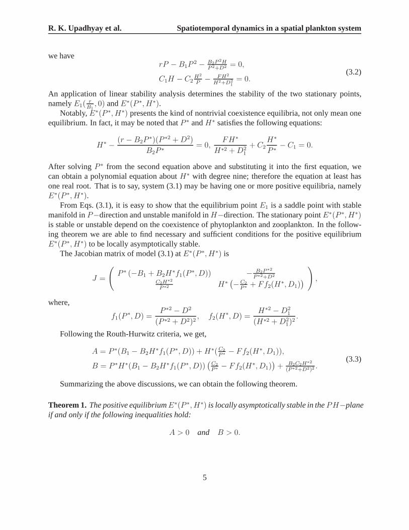
Fig.1 shows the dynamics of system (3.1) that for increasingfish predation rates atF = 0 (limitcycle—no fish),F = 0.02, 0.03, 0.04 (limit cycle) andF = 0.044 (phytoplankton dominance).We observe the limit cycle behavior for the fish predation rateF in the range0 ≤ F ≤ 0.043, andfor higher values phytoplankton dominance is reported for anon-spatial system (3.1).

Figure 1: (a) predator-prey zero-isoclines (b) prey zero-isoclines for different value ofF withparameters valuer = 1, B1 = 0.2, B2 = 0.91, C1 = 0.22, C2 = 0.2, D2 = 0.3, D1 = 0.1.

3.2. Global stability analysis

In order to study the global behavior of the positive equilibriumE∗(P ∗, H∗), we need the followinglemma which establishes a region for attraction for model system (3.1).

Lemma 1. The setR = (P,H) : 0 ≤ P ≤ rB1

, 0 ≤ H ≤ rC1

C2B1

is a region of attraction for allsolutions initiating in the interior of the positive quadrantR.

Theorem 3. IfP ∗(r − B1P

∗)2 < 4B1rD2, rC1H

∗ < D21C2B1 (3.5)

hold, thenE∗ is globally asymptotically stable with respect to all solutions in the interior of thepositive quadrantR.

6


Proof. Let us choose a Lyapunov function

V (P,H) =

∫ P

P ∗

ξ − P ∗

ξϕ(ξ)dξ + w

∫ H

H∗

η −H∗

ηdη, (3.6)

whereϕ(P ) = B2P2

P 2+D2 .Differentiating both sides with respect tot, we get

dV

dt(P,H) =

P − P ∗

Pϕ(P )

dP

dt+ w

H −H∗

H

dH

dt,

Substituting the expressions ofdPdt

and dHdt

from Eq. (3.1) and puttingw = P ∗

C2H∗, we obtained:

dVdt

= P−P ∗

P

(

rP−B1P2

ϕ(P )−H∗

)

− (H −H∗)2 P ∗

H∗P− w(H −H∗)2

F (D2

1−H∗H)

(H2+D2

1)(H∗2+D2

1)

= (P−P ∗)2

BP 2P ∗

(

rP ∗P − rD2 − B1PP ∗(P ∗ + P ))

− (H −H∗)2 P ∗

H∗P

−w(H −H∗)2F (D2

1−H∗H)

(H2+D2

1)(H∗2+D2

1)

then dVdt

< 0 for all P,H ∈ R if the condition (3.5) hold.

4. Stability analysis of the spatial model system

In this section, we study the effect of diffusion on the modelsystem about the interior equilibriumpoint. Complex marine ecosystems exhibit patterns that arebound to each other yet observed overdifferent spatial and time scales (Grimm et al., 2005). Turing instability can occur for the modelsystem because the equation for predator is nonlinear with respect to predator population,H andunequal values of diffusive constants. To study the effect of diffusion on the system (3.1), wederive conditions for stability analysis in one and two dimensional cases.

4.1. One dimensional case

The model system (2.1) in the presence of one-dimensional diffusion has the following form:

∂P∂t

= rP −B1P2 − B2P

2HP 2+D2 + d1

∂2P∂x2 ,

∂H∂t

= C1H − C2H2

P− FH2

H2+D2

1

+ d2∂2H∂x2 .

(4.1)

To study the effect of diffusion on the model system, we have considered the linearized formof system aboutE∗(P ∗, H∗) as follows:

∂U∂t

= b11U + b12V + d1∂2U∂x2 ,

∂V∂t

= b21U + b22V + d2∂2V∂x2 ,

(4.2)

7


whereP = P ∗ + U,H = H∗ + V and

b11 = −P ∗(B1 − B2H∗f1(P

∗, D)), b12 = −B2P∗/(P ∗2 +D2),

b21 = C2H∗2/P ∗2, b22 = H∗(Ff2(H

∗, D1)− C2/P∗).

It may be noted that(U, V ) are small perturbations of(P,H) about the equilibrium pointE∗(P ∗, H∗).

In this case, we look for eigenfunctions of the form

∞∑

n=0

(

anbn

)

exp (λt+ ikx),

and thus solutions of system (4.2) of the form

(

U

V

)

=∞∑

n=0

(

anbn

)

exp (λt+ ikx),

whereλ andk are the frequency and wave-number respectively. The characteristic equation of thelinearized system (4.2) is given by

λ2 + ρ1λ+ ρ2 = 0, (4.3)

whereρ1 = A + (d1 + d2)k

2, (4.4)

ρ2 = B + d1d2k4 +

[

d2P∗(B1 − B2H

∗f1(P∗, D)) + d1H

∗(C2/P∗ − Ff2(H

∗, D1))]

k2, (4.5)

whereA andB are defined in Eq. (3.3). From Eqs. (4.3)—(4.5), and using Routh-Hurwitz criteria,we can know that the positive equilibriumE∗ is locally asymptotically stable in the presence ofdiffusion if and only if

ρ1 > 0 and ρ2 > 0. (4.6)

Summarizing the above discussions, we can get the followingtheorem immediately.

Theorem 4. (i) If the inequalities in Eq.(3.4)are satisfied, then the positive equilibrium pointE∗

is locally asymptotically stable in the presence as well as absence of diffusion.(ii) Suppose that inequalities in Eq.(3.4)are not satisfied, i.e., eitherA or B is negative or both

A andB are negative. Then for strictly positive wave-numberk > 0, i.e., spatially inhomogeneousperturbations, by increasingd1 andd2 to sufficiently large values,ρ1 andρ2 can be made positiveand henceE∗ can be made locally asymptotically stable.

Diffusive instability sets in when at least one of the conditions in Eq. (4.6) is violated subjectto the conditions in Theorem 1. But it is evident that the firstconditionρ1 > 0 is not violated when

8


the conditionA > 0 is met. Hence only the violation of conditionρ2 > 0 gives rise to diffusioninstability. Hence the condition for diffusive instability is given by

H(k2) = d1d2k4 +

[

d2P∗(B1 − B2H

∗f1(P∗, D)) + d1H

∗(C2/P∗ − Ff2(H

∗, D1))]

k2 +B < 0.

(4.7)H is quadratic ink2 and the graph ofH(k2) = 0 is a parabola. The minimum ofH(k2) occurs atk2 = k2

m where

k2m =

1

2d1d2

[

d2P∗(B2H

∗f1(P∗, D)− B1) + d1H

∗(Ff2(H∗, D1)− C2/P

∗)]

> 0. (4.8)

Consequently the condition for diffusive instability isH(k2m). Therefore

1

4d1d2

[

d2P∗(B2H

∗f1(P∗, D)− B1) + d1H

∗(Ff2(H∗, D1)− C2/P

∗)]

> B. (4.9)

Theorem 5. The criterion for diffusive instability for the model system is obtained by combiningthe result of Theorem 1,(4.8)and (4.9)and leading to the following condition:

d2P∗(B2H

∗f1(P∗, D)−B1) + d1H

∗(Ff2(H∗, D1)− C2/P

∗ > 2(Bd1d2)1

2 > 0. (4.10)

In the following theorem, we are able to show the global stability behaviour of the positiveequilibrium in the presence of diffusion.

Theorem 6. (i) If the equilibriumE∗ of system(3.1) is globally asymptotically stable, the corre-sponding uniform steady state of system(4.2) is also globally asymptotically stable.

(ii) If the equilibriumE∗ of system(3.1) is unstable even then the corresponding uniform steadystate of system(4.2)can be made globally asymptotically stable by increasing the diffusion coeffi-cientd1 andd2 to a sufficiently large value for strictly positive wave-numberk > 0.

Proof. For the sake of simplicity, letP (x, t) = P,H(x, t) = H. Forx ∈ [0, R] andt ∈ [0,∞], letus define a functional:

V1 =

∫ R

0

V (P,H)dx

whereV (P,H) is defined as Eq. (3.6).DifferentiatingV1 with respect to timet along the solutions of system (4.2), we get

dV1

dt=

∫ R

0

(∂V

∂P

∂P

∂t+

∂V

∂H

∂H

∂t

)

dx =

∫ R

0

dV

dtdx+

∫ R

0

(

d1∂V

∂P

∂2P

∂x2+ d2

∂V

∂H

∂2H

∂x2

)

dx.

Using the boundary condition (2.3), we obtain

dV1

dt=

∫ R

0

dV

dtdx−d1

∫ R

0

P ∗(P 2 + 3D2)− 2D2P

B2P 4

(∂P

∂x

)2

dx−d2

∫ R

0

wH∗

H2

(∂H

∂x

)2

dx. (4.11)

From Eq. (4.11), we note that ifdVdt

< 0 then dV1

dtin the interior of the positive quadrant of the

PH−plane, and hence the first part of the theorem follows. We alsonote that ifdVdt

< 0 then dV1

dt

can be made negative by increasingd1 andd2 a sufficiently large value, and hence the second partof the theorem follows.

9


4.2. Two dimensional case

In two-dimensional case, the model system (2.1) can be written as

∂P∂t

= rP −B1P2 − B2P

2HP 2+D2 + d1

(

∂2P∂x2 + ∂2P

∂y2

)

,

∂H∂t

= C1H − C2H2

P− FH2

H2+D2

1

+ d2

(

∂2H∂x2 + ∂2H

∂y2

)

.(4.12)

In this section, we show that the result of theorem 5 remain valid for two dimensional case. Toprove this result we consider the following functional (Dubey and Hussain, 2000):

V2 =

∫∫

Ω

V (P,H)dA

whereV (P,H) is defined as Eq. (3.6).DifferentiatingV2(t) with respect to timet along the solutions of system (4.12), we obtain

dV2

dt= I1 + I2, (4.13)

where

I1 =

∫∫

Ω

dV

dtdA, I2 =

∫∫

Ω

(

d1∂V

∂P∇2P + d2

∂V

∂H∇2H

)

dA.

Using Green’s first identity in the plane∫∫

Ω

F∇2GdA =

∫

∂Ω

F∂G

∂nds−

∫∫

Ω

(∇F · ∇G)dA.

and under an analysis similar to Dubey and Hussain(2000), one can show that

d1

∫∫

Ω

(

∂V

∂P∇2P

)

dA = −d1

∫∫

Ω

∂2V

∂P 2

[

(∂P

∂x)2 + (

∂P

∂y)2]

dA ≤ 0,

d2

∫∫

Ω

(

∂V

∂H∇2H

)

dA = −d2

∫∫

Ω

∂2V

∂H2

[

(∂H

∂x)2 + (

∂H

∂y)2]

dA ≤ 0.

This shows thatI2 ≤ 0. From the above analysis we note that ifI1 < 0, thendV2

dt. This implies that

if in the absence of diffusionE∗ is globally asymptotically stable, then in the presence of diffusionE∗ will remain globally asymptotically stable.

We also note that ifdVdt

> 0, thenI1 > 0. In such a case diffusion,E∗ will be unstable in theabsence of diffusion. Even in this case by increasingd1 andd2 to a sufficiently large valuedV2

dtcan

be made negative. This shows that if in the absence of diffusionE∗ is unstable, then in the presenceof diffusionE∗ can be made stable by increasing diffusion coefficients to sufficiently large value.

10


5. Numerical simulations

In this section, we perform numerical simulations to illustrate the results obtained in previous sec-tions. The dynamics of the model system (2.1) is studied withthe help of numerical simulation,both in one and two dimensions, to investigate the spatiotemporal dynamics of the model sys-tem (2.1). For the one-dimensional case, the plots (space vs. population densities) are obtained tostudy the spatial dynamics of the model system. The temporaldynamics is studied by observingthe effect of time on space vs. density plot of prey populations. For the two-dimensional case, thespatial snapshots of prey densities are obtained at different time levels for different values ofFand we have tried to study the spatiotemporal dynamics of thespatial model system. The rate offish predation,F acting as forcing term or distributed control parameter in the model system (2.1)which is strictly nonnegative. Mathematically, we assume thatF can be manipulated at every pointin space and time. However, from practical point of view, we only have direct control of the netdensity of fish population at any instant. The parameters determining the shape of the type-IIIfunctional response of fish to zooplankton density are set more or less arbitrarily. They will in factvery much depend on the fish species, and also change significantly within a species with the sizeof the individuals.

5.1. Spatiotemporal dynamics in One-dimensional system

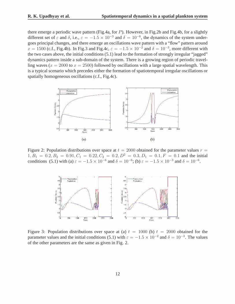
Now we start our insight into the spatiotemporal dynamics ofthe model system (2.1) in one-dimension with the following set of parameter values. The spatiotemporal dynamics of the systemdepends to a large extent on the choice of initial conditions. In a real aquatic ecosystem, thedetails of the initial spatial distribution of the species can be caused by spatially homogenousinitial conditions. However, in this case, the distribution of species would stay homogenous forany time, and no spatial pattern can emerge. To get a nontrivial spatiotemporal dynamics, wehave perturbed the homogenous distribution. We start with ahypothetical “constant-gradient”distribution (Malchow et al., 2008):

P (x, 0) = P ∗, H(x, 0) = H∗ + εx+ δ, (5.1)

whereε andδ are parameters.(P ∗, H∗) = (1.8789, 1.3984) is the non-trivial equilibrium point ofsystem (3.1), with fixed parameter set

r = 1, B1 = 0.2, B2 = 0.91, C1 = 0.22, C2 = 0.2, D2 = 0.3, D1 = 0.1, F = 0.1.

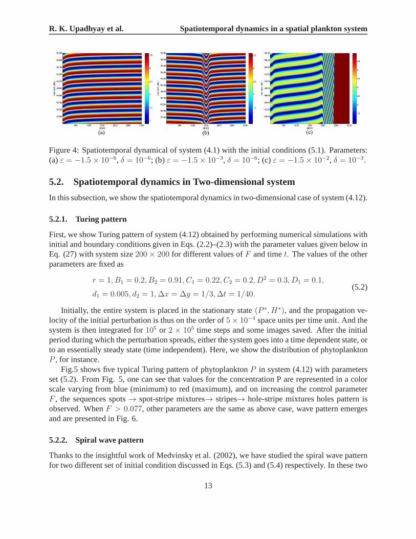
It appears that the type of the system dynamics depends onε andδ. In Figs. 2 and 3, weshow the population distribution over space at timet = 2000 (Fig.2) andt = 1000, 2000(Fig.3),respectively. In Fig. 4, we illustrate the pattern formation about the above two cases, the systemsize is 3000, iteration numbers from 17800 to 19800, i.e., time t from 1780 to 1980. In Fig.2aand Fig.4a,ε = −1.5 × 10−6 andδ = 10−6, the spatial distributions gradually vary in time, andthe local temporal behavior of the dynamical variablesP andH is strictly periodic following limitcycle of the non-spatial system, which is perhaps what is intuitively expected from system (4.1),

11


there emerge a periodic wave pattern (Fig.4a, forP ). However, in Fig.2b and Fig.4b, for a slightlydifferent set ofε andδ, i.e.,ε = −1.5 × 10−3 andδ = 10−6, the dynamics of the system under-goes principal changes, and there emerge an oscillations wave pattern with a “flow” pattern aroundx = 1500 (c.f., Fig.4b). In Fig.3 and Fig.4c,ε = −1.5 × 10−2 andδ = 10−3, more different withthe two cases above, the initial conditions (5.1) lead to theformation of strongly irregular “jagged”dynamics pattern inside a sub-domain of the system. There isa growing region of periodic travel-ling waves (x = 2000 to x = 2500) followed by oscillations with a large spatial wavelength.Thisis a typical scenario which precedes either the formation ofspatiotemporal irregular oscillations orspatially homogeneous oscillations (c.f., Fig.4c).

Figure 2: Population distributions over space att = 2000 obtained for the parameter valuesr =1, B1 = 0.2, B2 = 0.91, C1 = 0.22, C2 = 0.2, D2 = 0.3, D1 = 0.1, F = 0.1 and the initialconditions (5.1) with (a)ε = −1.5× 10−6 andδ = 10−6; (b) ε = −1.5× 10−3 andδ = 10−6.

Figure 3: Population distributions over space at (a)t = 1000 (b) t = 2000 obtained for theparameter values and the initial conditions (5.1) withε = −1.5 × 10−2 andδ = 10−3. The valuesof the other parameters are the same as given in Fig. 2.

12


Figure 4: Spatiotemporal dynamical of system (4.1) with theinitial conditions (5.1). Parameters:(a)ε = −1.5 × 10−6, δ = 10−6; (b) ε = −1.5× 10−3, δ = 10−6; (c) ε = −1.5× 10−2, δ = 10−3.

5.2. Spatiotemporal dynamics in Two-dimensional system

In this subsection, we show the spatiotemporal dynamics in two-dimensional case of system (4.12).

5.2.1. Turing pattern

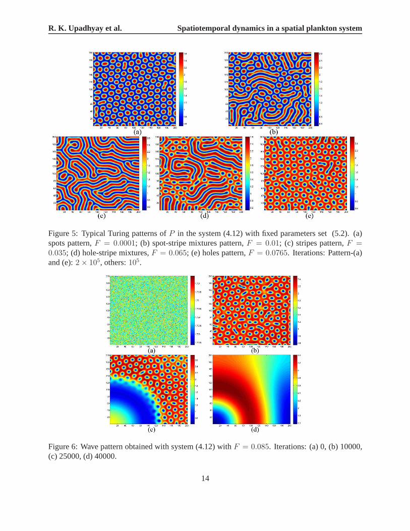
First, we show Turing pattern of system (4.12) obtained by performing numerical simulations withinitial and boundary conditions given in Eqs. (2.2)–(2.3) with the parameter values given below inEq. (27) with system size200 × 200 for different values ofF and timet. The values of the otherparameters are fixed as

r = 1, B1 = 0.2, B2 = 0.91, C1 = 0.22, C2 = 0.2, D2 = 0.3, D1 = 0.1,

d1 = 0.005, d2 = 1,∆x = ∆y = 1/3,∆t = 1/40.(5.2)

Initially, the entire system is placed in the stationary state (P ∗, H∗), and the propagation ve-locity of the initial perturbation is thus on the order of5× 10−4 space units per time unit. And thesystem is then integrated for105 or 2 × 105 time steps and some images saved. After the initialperiod during which the perturbation spreads, either the system goes into a time dependent state, orto an essentially steady state (time independent). Here, weshow the distribution of phytoplanktonP , for instance.

Fig.5 shows five typical Turing pattern of phytoplanktonP in system (4.12) with parametersset (5.2). From Fig. 5, one can see that values for the concentration P are represented in a colorscale varying from blue (minimum) to red (maximum), and on increasing the control parameterF , the sequences spots→ spot-stripe mixtures→ stripes→ hole-stripe mixtures holes pattern isobserved. WhenF > 0.077, other parameters are the same as above case, wave pattern emergesand are presented in Fig. 6.

5.2.2. Spiral wave pattern

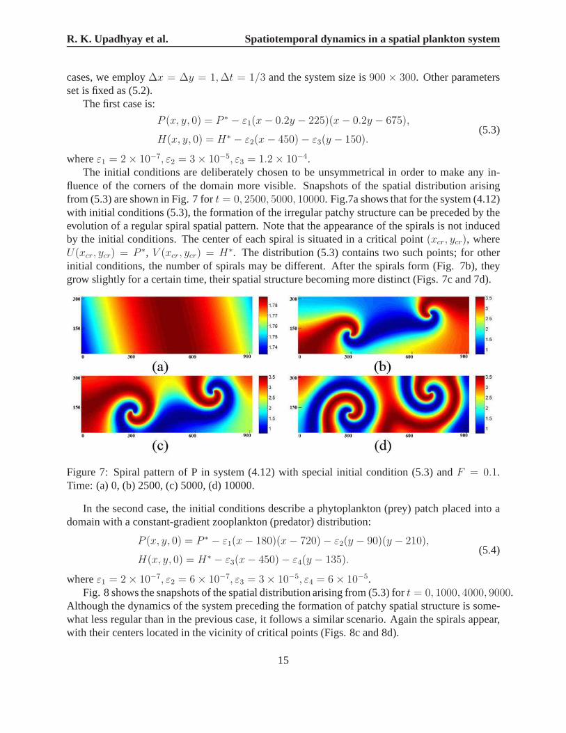
Thanks to the insightful work of Medvinsky et al. (2002), we have studied the spiral wave patternfor two different set of initial condition discussed in Eqs.(5.3) and (5.4) respectively. In these two

13


Figure 5: Typical Turing patterns ofP in the system (4.12) with fixed parameters set (5.2). (a)spots pattern,F = 0.0001; (b) spot-stripe mixtures pattern,F = 0.01; (c) stripes pattern,F =0.035; (d) hole-stripe mixtures,F = 0.065; (e) holes pattern,F = 0.0765. Iterations: Pattern-(a)and (e):2× 105, others:105.

Figure 6: Wave pattern obtained with system (4.12) withF = 0.085. Iterations: (a) 0, (b) 10000,(c) 25000, (d) 40000.

14


cases, we employ∆x = ∆y = 1,∆t = 1/3 and the system size is900 × 300. Other parametersset is fixed as (5.2).

The first case is:

P (x, y, 0) = P ∗ − ε1(x− 0.2y − 225)(x− 0.2y − 675),

H(x, y, 0) = H∗ − ε2(x− 450)− ε3(y − 150).(5.3)

whereε1 = 2× 10−7, ε2 = 3× 10−5, ε3 = 1.2× 10−4.The initial conditions are deliberately chosen to be unsymmetrical in order to make any in-

fluence of the corners of the domain more visible. Snapshots of the spatial distribution arisingfrom (5.3) are shown in Fig. 7 fort = 0, 2500, 5000, 10000. Fig.7a shows that for the system (4.12)with initial conditions (5.3), the formation of the irregular patchy structure can be preceded by theevolution of a regular spiral spatial pattern. Note that theappearance of the spirals is not inducedby the initial conditions. The center of each spiral is situated in a critical point(xcr, ycr), whereU(xcr, ycr) = P ∗, V (xcr, ycr) = H∗. The distribution (5.3) contains two such points; for otherinitial conditions, the number of spirals may be different.After the spirals form (Fig. 7b), theygrow slightly for a certain time, their spatial structure becoming more distinct (Figs. 7c and 7d).

Figure 7: Spiral pattern of P in system (4.12) with special initial condition (5.3) andF = 0.1.Time: (a) 0, (b) 2500, (c) 5000, (d) 10000.

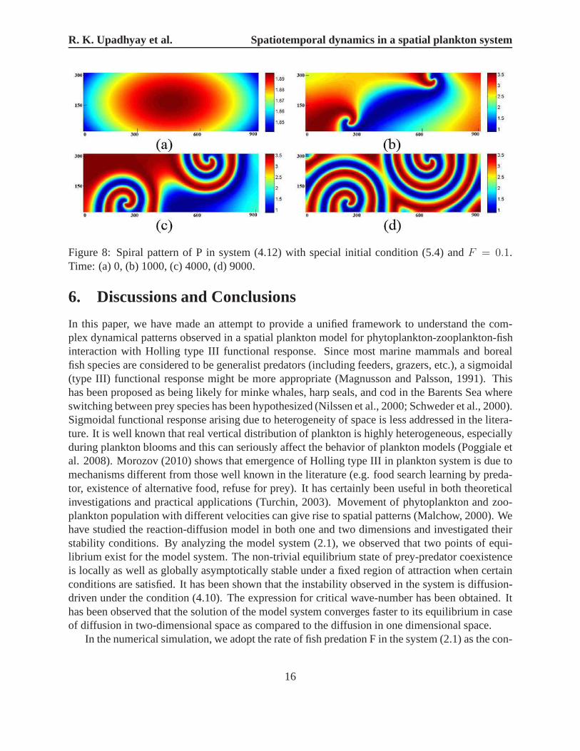
In the second case, the initial conditions describe a phytoplankton (prey) patch placed into adomain with a constant-gradient zooplankton (predator) distribution:

P (x, y, 0) = P ∗ − ε1(x− 180)(x− 720)− ε2(y − 90)(y − 210),

H(x, y, 0) = H∗ − ε3(x− 450)− ε4(y − 135).(5.4)

whereε1 = 2× 10−7, ε2 = 6× 10−7, ε3 = 3× 10−5, ε4 = 6× 10−5.Fig. 8 shows the snapshots of the spatial distribution arising from (5.3) fort = 0, 1000, 4000, 9000.

Although the dynamics of the system preceding the formationof patchy spatial structure is some-what less regular than in the previous case, it follows a similar scenario. Again the spirals appear,with their centers located in the vicinity of critical points (Figs. 8c and 8d).

15


Figure 8: Spiral pattern of P in system (4.12) with special initial condition (5.4) andF = 0.1.Time: (a) 0, (b) 1000, (c) 4000, (d) 9000.

6. Discussions and Conclusions

In this paper, we have made an attempt to provide a unified framework to understand the com-plex dynamical patterns observed in a spatial plankton model for phytoplankton-zooplankton-fishinteraction with Holling type III functional response. Since most marine mammals and borealfish species are considered to be generalist predators (including feeders, grazers, etc.), a sigmoidal(type III) functional response might be more appropriate (Magnusson and Palsson, 1991). Thishas been proposed as being likely for minke whales, harp seals, and cod in the Barents Sea whereswitching between prey species has been hypothesized (Nilssen et al., 2000; Schweder et al., 2000).Sigmoidal functional response arising due to heterogeneity of space is less addressed in the litera-ture. It is well known that real vertical distribution of plankton is highly heterogeneous, especiallyduring plankton blooms and this can seriously affect the behavior of plankton models (Poggiale etal. 2008). Morozov (2010) shows that emergence of Holling type III in plankton system is due tomechanisms different from those well known in the literature (e.g. food search learning by preda-tor, existence of alternative food, refuse for prey). It hascertainly been useful in both theoreticalinvestigations and practical applications (Turchin, 2003). Movement of phytoplankton and zoo-plankton population with different velocities can give rise to spatial patterns (Malchow, 2000). Wehave studied the reaction-diffusion model in both one and two dimensions and investigated theirstability conditions. By analyzing the model system (2.1),we observed that two points of equi-librium exist for the model system. The non-trivial equilibrium state of prey-predator coexistenceis locally as well as globally asymptotically stable under afixed region of attraction when certainconditions are satisfied. It has been shown that the instability observed in the system is diffusion-driven under the condition (4.10). The expression for critical wave-number has been obtained. Ithas been observed that the solution of the model system converges faster to its equilibrium in caseof diffusion in two-dimensional space as compared to the diffusion in one dimensional space.

In the numerical simulation, we adopt the rate of fish predation F in the system (2.1) as the con-

16


trol parameter which is strictly nonnegative. In the two-dimensional case, on increasing the valueof F , the sequences spots→spot-stripe mixtures→stripes→ hole-stripe mixtures→holes→wavepattern is observed. For the sake of learning the wave pattern further, we show the time evolutionprocess of the pattern formation with two special initial conditions and find spiral wave patternemerge. That is to say, our two-dimensional spatial patterns may indicate the vital role of phasetransience regimes in the spatiotemporal organization of the phytoplankton and zooplankton in theaquatic systems. It is also important to distinguish between “intrinsic” patterns, i.e., patterns aris-ing due to trophic interaction such as those considered above, and “forced” patterns induced bythe inhomogeneity of the environment. The physical nature of the environmental heterogeneity,and thus the value of the dispersion of varying quantities and typical times and lengths, can beessentially different in different cases.

Acknowledgements

This work is supported by University Grants Commission, Govt. of India under grant no. F.33-116/2007(SR) to the corresponding author (RKU) who has visited to Budapest, Hungary underIndo-Hungarian Educational exchange programme. Authors are also grateful to Dr. Sergei V.Petrovskii and the reviewer for their critical review and helpful suggestions.

References

[1] M. Abbott. Phytoplankton patchiness: ecological implications and observation methodsIn:Patch dynamics (Levin, S. A., Powell, T. M. and Steele, J. H.,eds.), Lecture Notes inBiomath. 96(1993), 37-49.

[2] A. D. Bazykin, A.I. Khibnik, B. Krauskopf, B. Nonlinear dynamics of interacting popula-tions. World Scientific, Singapore, 1998.

[3] B. Chen,M. Wang. 2008.Qualitative analysis for a diffusive predator-prey model.Comp.Math. with Appl. 55(2008), 339-355.

[4] B. Dubey, J. Hussain.Modelling the interaction of two biological species in polluted environ-ment.J. Math. Anal. Appl. 246(2000), 58-79.

[5] M. J. R. Fasham.The statistical and mathematical analysis of plankton patchiness.Oceanogr.Mar. Biol. Annu. Rev 16(1978), 43-79.

[6] C. Fu, R. Mohn, L.P. Fanning.Why the Atlantic cod stock off eastern Nova Scotia has notrecovered.Can. J. Fish. Aquat. Sci 58(2001), 1613-1623.

[7] H. Gao, H. Wei, W. Sun, X. Zhai.Functions used in biological models and their influence onsimulations.Indian J. Marine Sci. 29(2000), 230-237.

17


[8] C.H. Greene, E. A. Widder, M. J. Youngbluth, A. Tamse, G. E. Johnson.The migration be-havior, fine structure and bioluminescent activity of krillsound-scattering layers.Limnologyand Oceanography 37(1992), 650-658.

[9] V. Grimm, E. Revilla, U. Berger, F. Jeltsch, W. Mooij, S. Railsback, H. Thulke, J. Weiner,T. Wiegand, D. DeAngelis,Pattern-oriented modeling of agent-based complex systems:lessons from ecology, Science 310 (2005), 987–991.

[10] A.C. Hammer, J.W. Pitchford.The role of mixotrophy in plankton bloom dynamics and theconsequences for productivity.ICES J. Marine Sci. 62(2005), 833-840.

[11] T.K. Kar, H. Matsuda.Global dynamics and controllability of a harvested prey-predator sys-tem with Holling type III functional response.Nonlinear Anal.: Hybrid Systems 1(2007),59-67.

[12] M. Liermann, R. Hilborn.Depensation: Evidence, models and implications.Fish and Fish-eries 2(2001), 33-58.

[13] C. Loehle.Challenges of ecological complexity.Ecological Complexity 1(2004), 3-6.

[14] D. Ludwig, D. Jones, C. Holling.Qualitative analysis of an insect outbreak system: thespruce budworm and forest.J. Animal Eco. 47(1978), 315-332.

[15] F. Mackas, C. M. Boyd. Spectral analysis of zooplanktonspatial heterogeneity. Science204(1979), 62-64.

[16] K. G. Magnusson, O.K. Palsson.Predator-prey interactions of cod and capelin in Icelandicwaters.ICES Marine Science Symposium. 193(1991), 153-170.

[17] H. Malchow. 1993.Spatio-temporal pattern formation in nonlinear nonequilibrium planktondynamics.P ROY SOC LOND B 251(251), 103-109.

[18] H. Malchow.Nonlinear plankton dynamics and pattern formation in an ecohydrodynamicmodel system.J. Marine Systems, 7(1996), 193-202.

[19] H. Malchow.Non-equilibrium spatio-temporal patterns in models of non-linear plankton dy-namics.Freshwater Biol. 45(2000), 239-251.

[20] H. Malchow, S. V. Petrovskii, A. B. Medvinsky.Numerical study of plankton-fish dynamicsin a spatially structured and noisy environment.Ecol. Model. 149(2002), 247-255.

[21] H. Malchow, S. V. Petrovskii, E. Venturino. Spatiotemporal Patterns in Ecology and Epidemi-ology: Theory, Models and Simulation, CRC Press, UK, 2008.

[22] R. M. May. Stability and Complexity in model ecosystems, Princeton University press,Princeton, NJ. 1973.

18


[23] A. B. Medvinsky, S. V. Petrovskii, I. A. Tikhonova, H. Malchow, B.-L. Li. Spatiotemporalcomplexity of plankton and fish dynamics.SIAM Review. 44(2002), 311-370.

[24] A. B. Medvinsky, S. V. Petrovskii, I. A. Tikhonova, E. Venturino, H. Malchow.Chaos andregular dynamics in a model multi-habitat plankton-fish community.J. Biosciences 26(2001),109-120.

[25] A. B. Medvinsky, I. A. Tikhonova, R. R. Aliev, B. -L. Li, Z. S. Lin, H. Malchow.Patchyenvironment as a factor of complex plankton dynamics.Phys. Rev. E. 64(2001), 021915.

[26] L. Michaelis, M. L. Menten.Die Kinetik der Invertinwirkung.Biochem. Z 49(1913), 333-369.

[27] A. Morozov. Emergence of Holling type III zooplankton functional response: Bringing to-gether field evidence and mathematical modelling.J. Theor. Biol. 265(2010), 45-54.

[28] A. Morozov, E. Arashkevich, M. Reigstad, S. Falk-Petersen.Influence of spatial heterogene-ity on the type of zooplankton functional response: A study based on field observations.Deep-Sea Research II 55(2008), 2285-2291.

[29] J. D. Murray. Mathematical Biology, Springer-Verlag,New York, 1989.

[30] K. T. Nilssen, O.-P. Pedersen, L. Folkow, T. Haug.Food consumption estimates of BarentsSea harp seals.NAMMCO Scientific Publications 2(2000), 9-27.

[31] A. Okubo. Diffusion and ecological problems: mathematical models, Springer-Verlag,Berlin. 1980.

[32] M. Pascual. 1993.Diffusion-induced chaos in a spatial predator-prey system. P ROY SOC B251(1993), 1-7.

[33] S. V. Petrovskii, H. Malchow.Critical phenomena in plankton communities: KISS modelrevisited.Nonlinear Anal.: RWA 1(2000), 37-51.

[34] S. V. Petrovskii, H. Malchow.Wave of chaos: new mechanism of pattern formation in spatio-temporal population dynamics.Theor. Popul. Biol. 59(2001), 157-174.

[35] J. -C. Poggiale, M. Gauduchon, P. Auger.Enrichment paradox induced by spatial heterogene-ity in a phytoplankton- zooplankton system.Math. Mod. Natu. Phenom. 3(2008), 87-102.

[36] L. A. Real.The kinetic of functional response.Am. Nat. 111(1977), 289-300.

[37] M. Scheffer. Ecology of shallow lakes, Chapman and Hall, London. 1998.

[38] M. Scheffer, R. J. De Boer.Implications of spatial heterogeneity for the paradox of enrich-ment.Ecology 76(1996), 2270-2277.

19


[39] T. Schweder, G. S. Hagen, E. Hatlebakk.Direct and indirect effects of minke whale abun-dance on cod and herring fisheries: A scenario experiment forthe Greater Barents Sea.NAMMCO Scientific Publications 1(2000), 120-133.

[40] L. A. Segel, J. L. Jackson.Dissipative structure: An explanation and an ecological example.J. Theo. Biol. 37(1972), 545-559.

[41] J. A. Sherratt, B. T. Eagan, M. A. Lewis.Oscillations and chaos behind predator-prey inva-sion: mathematical artifact or ecological reality?Phil. Trans. Roy. Soc. Lond. B 352(1997),21-38.

[42] J. A. Sherratt, M. A. Lewis, A. C. Fowler.Ecological chaos in the wake of invasion.PNAS92(1995), 2524-2528.

[43] J. H. Steele. Spatial pattern in plankton communities,Plenum Press, New York, 1978.

[44] J. H. Steele, E. W. Henderson.A simple plankton model.Am. Nat. 117(1981), 676-691.

[45] J. H. Steele, E. W. Henderson.A simple model for plankton patchiness.J. Plankton Research14(1992), 1397-1403.

[46] J. H. Steele, E. W. Henderson.The role of predation in plankton models.J. Plankton Research,14(1992), 157-172.

[47] J. E. Truscott, J. Brindley.Equilibria, stability and excitability in a general class of planktonpopulation models.Phil. Trans. Roy. Soc. Lond. A 347(1994), 703-718.

[48] J. E. Truscott, J. Brindley.Ocean plankton populations as excitable media.Bull. Math. Biol.56(1994), 981-998.

[49] P. Turchin. Complex Population Dynamics: A Theoretical/Empirical Synthesis. PrincetonUniversity Press, Princeton, NJ, 2003.

[50] R. K. Upadhyay, N. Kumari, V. Rai.Wave of chaos and pattern formation in a spatialpredator-prey system with Holling type IV functional response.Math. Mod. Natu. Phenom.3(2008), 71-95.

[51] R. K. Upadhyay, N. Kumari, V. Rai.Wave of chaos in a diffusive system: Generating realisticpatterns of patchiness in plankton-fish dynamics.Chaos Solit. Fract. 40(2009), 262-276.

[52] R. K. Upadhyay, N. K. Thakur, B. Dubey.Nonlinear non-equilibrium pattern formation in aspatial aquatic system: Effect of fish predation.J. Biol. Sys. 18(2010), 129-159.

[53] J. Xiao, H. Li, J. Yang, G. Hu.Chaotic Turing pattern formation in spatiotemporal systems.Frontier of Physics in China 1(2006), 204-208.

20


Appendix: Proof of Theorem 1

The Jacobian matrix of model (3.1) corresponding to the positive equilibriumE∗(P ∗, H∗) is givenby

J =

[

b11 b12b11 b11

]

,

whereb11 = r − 2B1P

∗ − 2B2D2P ∗H∗

(P ∗2+D2)2, b12 = − B2P

∗2

P ∗2+D2 ,

b21 =C2H

∗2

P ∗2 , b22 = C1 −2C2H

∗

P ∗−

2D2

1FH∗

(H∗2+D2

1)2.

SinceE∗(P ∗, H∗) is a solution of Eq. (3.2). From the first equation of Eq. (3.2), we obtain

r −B1P∗ =

B2P∗H∗

P ∗2 +D2,

So,b11 = r − 2B1P

∗ − 2B2D2P ∗H∗

(P ∗2+D2)2= −B1P

∗ + (r − B1P∗)− 2B2D

2P ∗H∗

(P ∗2+D2)2

= −B1P∗ + B2P

∗H∗

P ∗2+D2 − 2B2D2P ∗H∗

(P ∗2+D2)2= −B1P

∗ + B2P∗H∗(P ∗2

−D2)(P ∗2+D2)2

= P ∗(−B1 +B2H∗f1(P

∗, D))

where,f1(P ∗, D) = P ∗2−D2

(P ∗2+D2)2.

From the second equation of Eq. (3.2), we have

C1 −C2H

∗2

P ∗2=

FH∗

H∗2 +D21

.

Therefore,

b22 = C1 −2C2H

∗2

P ∗2 −2D2

1FH∗

(H∗2+D2

1)2

= −C2H∗2

P ∗2 +(

C1 −C2H

∗2

P ∗2

)

−2D2

1FH∗

(H∗2+D2

1)2

= −C2H∗2

P ∗2 + FH∗

H∗2+D2

1

−2D2

1FH∗

(H∗2+D2

1)2

= −C2H∗2

P ∗2 +FH∗(H∗2

−D2

1)

(H∗2+D2

1)2

= H∗

(

−C2

P ∗+ Ff2(H

∗, D1))

,

wheref2(H∗, D1) =(H∗2

−D2

1)

(H∗2+D2

1)2

.Now the characteristic equation corresponding to the matrix J is given by

λ2 − (b11 + b22)λ+ (b11b22 − b12b21) or λ2 + Aλ+B = 0,

whereA andB are defined in (3.3). By Routh-Hurwitz criteria, all eigenvalues ofJ will havenegative real parts if and only ifA > 0, B > 0. Thus, the theorem follows.

21

math. model. nat. phenom

Documents