T H O M A S D E M U Y N C K

M AT H - S - 4 0 0M AT H E M AT I C S A N DE C O N O M I C M O D E L L I N G

Contents

Logic and proofs 5

Sequences and limits 19

Functions 41

Extreme and intermediate value theorem 45

Correspondences 53

Berge’s maximum theorem 57

Convexity 61

Contraction mappings 65

Sperner’s lemma 69

Brouwer’s fixed point theorem 75

General equilibrium in exchange economies 79

4

Kakutani’s fixed point theorem 85

Existence Nash equilibrium 87

Logic and proofs

A teacher announces in class that an examination will be held on some day during the following week, and moreover that the examinationwill be a surprise. The students, having followed a course in mathematical logic argue that a surprise exam cannot occur. For suppose theexam were on the last day of the week. Then on the previous night, the students would be able to predict that the exam would occur on thefollowing day, and the exam would not be a surprise. So it is impossible for a surprise exam to occur on the last day. But then a surpriseexam cannot occur on the penultimate day, either, for in that case the students, knowing that the last day is an impossible day for a surpriseexam, would be able to predict on the night before the exam that the exam would occur on the following day. Similarly, the students arguethat a surprise exam cannot occur on any other day of the week either. Confident in this conclusion, they decide not to study for the exam.The next week, the teacher gives an exam on Wednesday, which, despite all the above, was an utter surprise to all students.

Timothy Y. Chow, The American Mathematical Monthly, Vol. 105, No. 1 (Jan., 1998)

Logic is the language of reasoning. It deals with the evaluationof arguments. Its main aim is to develop a system of methods andprinciples that can be used as a criteria for evaluating the validity ofcertain chains of arguments. Propositional logic, which is a subfieldof logic, is a logical system built around two values True and False,called the truth values. For simplicity we can assign the value 1 tosomething that is True and the value 0 to something that is False.1 1 We don’t allow for statements that can

be both true and false or for statementsthat are neither true nor false.

The aim of propositional logic is to find out the truth value of for-mula’s.

If p is a formula, and this formula is true, we write

T(p) = 1.

If the formula is false, we write

T(p) = 0.

The main objective of mathematics is to find (non trivial) formula’sthat are true. Many formulas are obtained by putting together ortransforming other formulas. In order to do this, however, we need togive the rules that determine how various formulas can be combinedinto other ones and how their truth value is determined. Also, as itis impossible to get something from nothing, we need some basicbuilding blocks. These building blocks are what we call atomicstatements.

6

An atomic statement, which we represent by the letters p, q, r, s, . . .,are the basic building blocks of a formula. Atomic statements are The following gives some examples of

atomic statements:

• p = “it is snowing”

• q = “all consumers are rational”

• r = “tax cuts increase welfare”

• s = “mathematics is boring”

either True or False. Every atomic statement is also a formula.

New formulas are build up from other formula’s. A first way totransform a given formula into another formula is by negation. If p isa formula then, ¬p is also a formula. Intuitively, ¬p means

“It is not the case that p”.Examples of negation are,

• ¬p = “it is not snowing.”

• ¬q = “not all consumers arerational.”

• ¬r = “a tax cut does not increaseswelfare.”

• ¬s = “mathematics is not boring.”

Of course p is true if and only if ¬p is false, as such, we obtain therule

T(¬p) = 1− T(p).

It is possible to represent this in a so called truth table. The firstcolumn of the truth table enumerates all possible values of the for-mula p. The second column enumerates the corresponding values of¬p.

p ¬p ¬(¬p)

1 0 1

0 1 0

Truth tables are useful because they allow us to derive equivalencebetween two expressions. The equivalence between the first and thirdcolumn for example shows that p ≡ ¬(¬p). For every possible truthvalue of p, p has the same truth value as ¬(¬(p))).2 2 In contrast to the English language,

mathematics has not problem withdouble negations.

Negation transforms one formula into another one. On the otherhand, it is also possible to combine two existing formulas into a newone. The first rule that does this is conjunction. If p and q are twoformulas then p ∧ q is also a formula and it means

“it is the case that p and q”.For example,

• p ∧ q = “it is snowing and allconsumers are rational.”

So the formula p ∧ q is assigned the truth value 1 if and only if boththe formula p is true and the formula q is true. In other words, p ∧ q isfalse if at least one of them is false. The mathematical rule is,3 3 Or equivalently,

T(p ∧ q) = min{T(p), T(q)}.T(p ∧ q) = 1 if and only if T(p) = 1 and T(q) = 1.

The following gives the truth table for p ∧ q. Here the first twocolumns give every possible combination of truth values for p and q.The third column gives the value of p ∧ q.

p q p ∧ q

1 1 1

1 0 0

0 1 0

0 0 0

7

The second rule to combine two formulas into a new one isdisjunction. If p and q are formula then p ∨ q is also a formula and itmeans that

“it is the case that p or q”

Here the “or” is inclusive, so either p is true, q is true or they areboth true. The mathematical rule is that,4 For example,

• p ∨ q = “it is snowing or all con-sumers are rational.”

4 Or equivalently,

T(p ∨ q) = max{T(p), T(q)}.

T(p ∨ q) = 1 if and only if T(p) = 1 or T(q) = 1.

The following truth table demonstrates that the ∨ rule can also bedefined by combining ∧ and ¬:

p ∨ q ≡ ¬(¬p ∧ ¬q).

p q p ∨ q ¬p ¬q ¬p ∧ ¬q ¬(¬p ∧ ¬q)

1 1 1 0 0 0 1

1 0 1 0 1 0 1

0 1 1 1 0 0 1

0 0 0 1 1 1 0

Observe that for any possible value combination of p and q, theformula p ∨ q has the same truth value as ¬(¬p ∧ ¬q). Equivalently,5 5 Notice the similarity with De Mor-

gan’s law:

(A ∪ B)c = Ac ∩ Bc.¬(p ∨ q) ≡ (¬p ∧ ¬q).

A third very important rule to combine two formula’s into a newone is by implication. If p and q are formula then p → q is also aformula and it means,

“If p, then q”.For example,

• p → q = “If it is snowing then allconsumers are rational.”

Here p → q is true if q is true whenever p is true. The mathematicalrule is,6

6 Or equivalently,

T(p→ q) = max{1−T(p), min{T(p), T(q)}}.T(p→ q) = 1 if and only if T(p) = 1 implies T(q) = 1.

So for p → q to hold either p is False, in which case q can either beTrue or False or p is True but in that case, q must also be True.

p q p→ q ¬q p ∧ ¬q ¬(p ∧ ¬q)

1 1 1 0 0 1

1 0 0 1 1 0

0 1 1 0 0 1

0 0 1 1 0 1

8

Above truth table shows that7 7 Notice the equivalence between

A ⊆ B,

and(A ∩ Bc) = ∅.

p→ q ≡ ¬(p ∧ ¬q).

This is the basic justification for a proof by contradiction. In order toshow that p implies q you start by assuming that both p holds andq does not hold. Next you use this to derive a contradiction, whichshows that ¬(p ∧ ¬q) is True. Exercise: show that for any formula

p ∨ ¬p is always True. This is calledthe law of the excluded middle. Somemathematicians actually contest thisrule. If you don’t agree with the law ofthe excluded middle, you can’t use aproof by contradiction.

A final rule to combine two formula’s into a third one is byequivalence. If p and q are formula then p↔ q is also a formula andit means,

“p if and only if q”.For example,

• p↔ q = “it is snowing if and only ifall consumers are rational.”

The mathematical rule is,8

8 Or equivalently,

T(p↔ q) = max{

min{T(p), T(q)},min{1− T(p), 1− T(q)}

}.

T(p↔ q) if and only if

(T(p) = 1 and T(q) = 1),or ,

(T(p) = 0 and T(q) = 0)

.

p q p↔ q p→ q q→ p (p→ q) ∧ (q→ p)

1 1 1 1 1 1

1 0 0 0 1 0

0 1 0 1 0 0

0 0 1 1 1 1

From this, we see that p ↔ q has the same truth value as (p →q) ∧ (q→ p). As such, in order to show the equivalence between twostatements you can show that the first implies the second and thesecond implies the first.

Predicate logic

Until now we have studied what is called propositional logic.Predicate logic builds upon propositional logic by introducing twoadditional symbols, called quantifiers, namely the existential (∃) anduniversal (∀) quantifiers. These quantifiers must be combined withvariables belonging to some particular set. Recall that,

• ∀a ∈ A : P(a) means “for all a in A such that P(a) . . . ”

• ∃a ∈ A : P(a) means “there exists an a in A such that P(a) . . . ”

• ∃!a ∈ A : P(a) means “ there exists a unique a in A such that P(a). . . ”

9

Observe that the ∀ quantifier works as a long chain of ∧ connectivesover all elements in some set A. If A = {a1, a2, . . . , an} then ,

∀a ∈ A : P(a)

is the same as,(P(a1) ∧ P(a2) ∧ . . . ∧ P(an)) .

On the other hand, the ∃ operator works as a long chain of ∨ connec-tives.

∃a ∈ A : P(a),

Is the same as,(P(a1) ∨ P(a2) ∨ . . . ∨ P(an)) .

In addition, the quantifiers also work on sets that are of infinite size,which is the main reason for using them.

In order to prove statements containing quantifiers, it can be usefulto know some propositions that are logical true (without going tooformal). The following two rules shows you how to negate a formulacontaining quantifiers.9 9 Notice the similarity with the equiva-

lence between

¬(p ∧ q ∧ r),

and(¬p ∨ ¬q ∨ ¬r)

and the equivalence between

¬(p ∨ q ∨ r),

and(¬p ∧ ¬q ∧ ¬r).

• ¬(∀a ∈ A : P(a)), is equivalent to ∃a ∈ A : ¬P(a).

• ¬(∃a ∈ A : P(a)), is equivalent to ∀a ∈ A : ¬P(a).

Independent of what formula P is, these statements are always true.“Not (for all a, P(a))” is equivalent as the statement “there exists ana ∈ A such that not P(a)”.

For example, let us negate

∀x∀y : ((x > 0) ∧ (y < 0))→ (xy < 0)

First we change the ∀ quantifiers into an ∃ quantifier. Next, wenegate the premises. This gives,

∃x∃y : ((x > 0) ∧ (y < 0) ∧ (xy ≥ 0).

Next, we can also combine ∀ and ∃ quantifiers if we have proposi-tions that use multiple variables

∀a ∈ A, ∃b ∈ B : P(a, b).

There is no problem in exchanging te two quantifiers if they are ofthe same type,

∀a, ∀b : P(a, b)↔ ∀b, ∀a : P(a, b).

10

However, one should be very careful when the quantifiers are ofdifferent types. It is true that

∃a ∈ A, ∀b ∈ B : P(a, b)→ ∀b ∈ B, ∃a ∈ A : P(a, b).

The opposite, however does not need to hold. The left hand sidemeans that you have to select one a and combine it with any b toevaluate P(a, b). As such, a should be independent of b. The righthand side means that for any b, you should find an a to evaluateP(a, b). As such, the choice of a may depend on the choice of b.10 10 The following example illustrates.

• ∀a ∈ Z, ∃b ∈ Z : a ≥ b is true but

• ∃b ∈ Z, ∀a ∈ Z : a ≥ b is false.Let us now have a look at how the quantifiers interact with thelogical connectives. Let P and Q be two propositions, then

∃a ∈ A : (P(a) ∨Q(a))↔ [(∃a ∈ A : P(a)) ∨ (∃a ∈ A : Q(a))].

If the left hand side is true, then there is an a such that P(a) or Q(a)is true. Of course the same a can be used on the right hand side toshow→. If the right hand side is true, then we know that either thereis an a such that P(a) holds or there is an a′ such that Q(a′) holds.Use a or a′ to make the left hand side valid.

The same equivalence result does not hold for the existentialqualifier and the connective ∧.

∃a ∈ A : (P(a) ∧Q(a))→ [(∃a ∈ A : P(a)) ∧ (∃a ∈ A : Q(a))].

To go from left to right, we do the same as before, i.e. we use the athat makes the left hand side true. However, this does not work inthe other way, since the a and a′ that make the right hand side truemay be different.11 11 See also Exercise 11 for a similar

results for the universal quantifier.

Proofs

All results in mathematics are obtained via proofs. There aredifferent kind of proofs according to the logical format that are usedto construct the proof.

The direct proof of showing p→ q is to find a set of ‘intermediate’formula’s p0, p1, . . . , pn such that pi → pi+1 for all i = 0, . . . , n− 1 andwhere p0 = p, pn = q. This gives a chain,

p→ p1 → p2 → . . .→ q.

As such, if p is True, it then follows that q must also be True. Con-sider the following assertion, that we want to prove.

11

“For all integers x, if x is odd, then x2 is also odd.”

The direct proof starts with the assumption, p0 = “x is odd” andcreates a chain of intermediate ‘truths’ which end by sentence q =

“x2 is odd”, we can use the following chain of reasoning,

p0: x is odd

p1: then, there is an integer n such that x = 2n + 1.12 12 Every odd number can be written astwo times a number plus one.

p2: then, x2 = (2n + 1)2,

p3: then, x2 = 4n2 + 4n + 1,13 13 Remember: (a + b)2 = a2 + 2ab + b2.

p4: then, x2 = 4(n2 + n) + 1,

p5: then, x2 = 2z + 1 where z = 2(n2 + n) is an integer,

q: then, x2 is odd.14 14 As x2 is two times a number plus one.

A proof by contrapositive relies on the equivalence betweenp→ q and ¬q→ ¬p, as illustrated in the following truth table.

p q p→ q ¬q ¬p ¬q→ ¬p

1 1 1 0 0 1

1 0 0 1 0 0

0 1 1 0 1 1

0 0 1 1 1 1

So, in order to show that p → q we can start with ¬q and use adirect proof to show that ¬p. Let us demonstrate this by proving thefollowing,

“If the sum of two integers x + y is even then either both integers x andy are even or both integers x and y are odd.”

A direct proof of this would be quite involved.15 However, we can 15 Try it.

easily proof the assertion by starting from the assumption that x andy are not of the same parity.

¬q: assume x and y don’t have the same parity,

q1: then, wlog assume x is odd and y is even,16 16 wlog is an abbreviation for ‘withoutloss of generality’.

q2: then, there are integers z and w such that x = 2z + 1 and y = 2w,

q3: then x + y = 2z + 2w + 1 = 2(z + w) + 1,

¬p: then, x + y is odd.

12

A proof by contradiction relies on the equivalence betweenp and ¬(¬p). In order to show that p is true, one starts from theassumption that ¬p is true. Then, you show that this leads to acontradiction,17 showing indeed that ¬(¬p) ≡ p is true. 17 In other words, you show that ¬p is

false.For an example, let’s demonstrate that,

“√

2 is irrational.”

A direct proof of this assertion would be very difficult. So let usproceed by contradiction.

¬p:√

2 is rational,

p1: then,√

2 = a/b where a and b are integers and not both even.18 18 Every rational number can be writtenas the ratio of two numbers that haveno common divisors (except 1).p2: then, b

√2 = a,

p3: then, b22 = a2,

p4: then, a2 is even,

p5: then, a is even,19 19 Follows from the previous proof.

p6: then, there is a number z such that a = 2z,

p7: then, a2 = 4z2,

p8: then, b2 = 2z2,

p9: then, b2 is even,

p10: then, b is even.

From this we see that p10 and p5 contradict p1, So√

2 is not rationalwhich shows that it is irrational.

A proof by contradiction can also be used to demonstrate animplication p → q. In this case, one starts from the assumption¬(p → q) and show that this leads to a contradiction. In addition,¬(p→ q) ≡ (¬q ∧ p) so one can start from the assumption that p and¬q are both true and use this to derive a contradiction.

Proof by induction is somewhat different form the proofs pre-sented above. It can be used if the proposition to be proven musthold for each value of a parameter that takes a value in the set ofnatural numbers, N0.

Assume that we want to proof that a formula p(n) is true for allnatural numbers n.20 The proof by induction starts by proving that 20 There also exists a proof technique

called transfinite induction. Here theinduction of over all ordinals. Theseordinals may contain numbers that arelarger than infinite. . .

p(1) holds. Then it goes on to show that p(k) → p(k + 1) for allnatural numbers k. From this, it can be concluded that p(n) holds forall natural numbers n.

p(1)→ p(2)→ . . .→ p(k)→ p(k + 1)→ . . . .

13

As an illustration, let us prove,

“For all natural numbers n: ∑ni=1 i = n(n+1)

2 .”

First p(1) requires us to demonstrate that ∑1i=1 i = 1 = 1(1 +

1)/2 = 1, so this is true. For the induction step let us assume thatp(k) holds, i.e. ∑k

i=1 i = k(k + 1)/2. We need to show that this implies

p(k + 1) ≡k+1

∑i=1

i = (k + 1)(k + 2)/2.

p(k): ∑ki=1 i = k(k + 1)/2,

p1(k): then, ∑k+1i=1 i = ∑k

i=1 i + (k + 1),

p2(k): then, ∑k+1i=1 i = k(k + 1)/2 + (k + 1),21 21 By the induction hypothesis.

p3(k): then, ∑k+1i=1 i = k(k+1)+2(k+1)

2 ,

p(k + 1): then, ∑k+1i=1 i = (k+1)(k+2)

2 .

Be very careful with proving statements using quantifiers ∀ and∃. For the universal quantifier you should check the propositionfor any element of the set. So you will work with variables. For theexistential quantifier, it could suffice to only give one example.

For example, in order to prove,

∀a ∈ Z : a2 ≥ 0,

we need to show that a2 ≥ 0 for all integers. One way to do this isto prove the statement for all non-negative numbers and prove thestatement for all negative numbers. In order to prove,

∃a ∈ Z : a2 = 9,

we only need to find one number for which the statement holds.22 22 In this case we can pick either a = 3or a = −3. However, we only need tofind one of the two cases in order toestablish the proof.Reference

• Appendix A1.3 of Simon and Blume, (1994), Mathematics forEconomists, W. W. Northon and Company, New York, London.

Exercises

1. Let p, q, and r be the following statements:

• p: Traveling to Mars is expensive.

• q: I will travel to Mars.

14

• r: I have money.

Express the following English sentences as symbolic expressions:

• I have no money and I will not travel to Mars.

• I have no money and travelling to Mars is expensive, or I willtravel to Mars.

• It is not true that, I have money and will travel to Mars.

• Travelling to Mars is not expensive and I will go to Mars, ortravelling to Mars is expensive and I will not go to Mars.

2. Construct truth tables for each of the following formulas.

• P ∧ (Q ∨ ¬P)

• ¬P→ Q

• Q ∨ ¬(P ∧Q)

• P→ ¬(P ∧Q)

• P→ (P ∧Q)

• Q→ (P→ Q)

• P ∧ ¬P

• (Q ∨ P) ∧ ¬P

3. Which of the following arguments are valid?

(a) If I’m rich then I’m happy. I am happy. Therefore, I am rich.

(b) If Sam drinks beer, he is at least 16 years old. Sam doesn’tdrink beer. Therefore, Sam is not yet 16 years old.

(c) If sheep are white, they are popular with shepherds. Smallsheep are unpopular with shepherds. Heavy sheep are small.Therefore, white sheep are not heavy.

(d) If I study, I will not fail MATH-S-400. If I don’t party toomuch, then I will study. I failed at MATH-S-400. Therefore, Ipartied too much.

4. There is a party tonight.

• John comes to the party if Mary or Ann comes.

• Ann comes to the party if Mary does not come.

• If Ann comes to the party, John does not.

Try to figure out who will come to the party.

15

5. For each of the following propositions, state the negation:

• x > 0 and y > 0

• All x satisfy x ≥ a

• Neither x nor y is less than 5.

• For each ε > 0 there exists a δ > 0 such that B is satisfied.

• ∀ε > 0, ∃n ∈N, ∀m ∈N, (m ≥ n)→ (|xm − a| < ε).

• Everyone loves somebody some of the time.

6. Consider the following statement: If inflation increases, thenunemployment decreases. Which of the following statements areequivalent to the given one?

• For employment to decrease, inflation must increase

• A sufficient condition for unemployment to decrease is thatinflation increases.

• Unemployment can only decrease if inflation increases.

• If unemployment does not decrease, then inflation does notincrease.

• A necessary condition for inflation to increase is that unemploy-ment decreases.

7. What is the negation of

• ∀m ∈N0, (∃k, n ∈N0 : m = nk)→ (k = 1∨ k = m).

• Do you know the meaning of this sentence?

8. Show that:

[∃a ∈ A : P(a)→ Q(a)],

↔,

[(∀a ∈ A : P(a))→ (∃a ∈ A : Q(a))].

9. The ϵ, δ formula for continuity is the following: A function f :A→ R is continuous at a ∈ A ⊆ R iff

∀ε > 0, ∃δ > 0, ∀x ∈ A : |x− a| < δ→ | f (x)− f (a)| < ε.

• Explain graphically what this means.

• What do we have to show if we want that f is discontinuous ina.

• Can we switch the ∀ε > 0 and ∃δ > 0 quantifiers?

16

10. Write the following in mathematical language: For any 2 integerswe have that their sum is even if they are both even.

11. Show the following:

• (∀a ∈ A : P(a) ∧Q(a))↔ [(∀a ∈ A : P(a)) ∧ (∀a ∈ A : Q(a))].

• (∀a ∈ A : P(a) ∨Q(a))← [(∀a ∈ A : P(a)) ∨ (∀a ∈ A : Q(a))].

12. Prove the statement. If 6 is a prime number, then 62 = 30.

13. Prove the statement: For all integers m and n, if m and n are oddintegers, then m + n is an even integer.

14. Prove the statement: For all integers m and n, if the product of mand n is even, then m is even or n is even.

15. Prove the statement: For all nonnegative real numbers a, b and c,if a2 + b2 = c2, then a + b ≥ c.

16. Prove the pigeonhole principle: If if k, n are integers and kn + 1objects (pigeons) are distributed into n boxes (pigeon holes), thensome box must contain at least k + 1 of the objects.

17. Use the pigeonhole principle above to show that if there are npeople who can shake hands with one another (where n > 1), thenthere is always a pair of people who will shake hands with thesame number of people.

18. Proof that there are infinitely many primes.

19. Show that for all n ∈N, n < 2n.

20. Show that ∑nt=1 2t = 2n+1 − 2.

21. What is wrong with the following proof by induction that allbutterflies have the same colour.

“If there is a single butterfly in the "group", then clearly all but-terflies in the group have the same colour. For the inductive step,assume that n butterflies always have the same colour. Considera group of n + 1 butterflies. First, exclude the last butterfly andlook only at the first n butterflies, which by induction must havethe same colour. Likewise, exclude the first butterfly, then all otherbutterflies must have the same colour. Conclude that the first but-terfly is of the same colour as the middle ones which has the samecolour as the last one. Hence, all butterflies have the same colour.”

17

22. The price of a stock is defined as the sum of the actualized valuesof the dividends. Suppose that the yearly dividend is K and theyearly interest rate is r. Prove that if we take n years into account,that the price of the stock is given by,

p =Kr

(1−

(1

1 + r

)n).

23. Show that there are two irrational numbers a and b such that ab

is rational.

Sequences and limits

We use standard notation as much as possible. The set R is theset of real numbers, N is the infinite set of strict positive integers{1, . . .}. Elements of these sets are sometimes called scalars and theyare denoted by small letters x, y, z, . . ..

The set Rk is the k-fold Cartesian product of R, elements of Rk arek-dimensional column vectors and they are denoted in bold, x, y, z . . .,e.g.,

x =

x1

x2...

xk

We use subindices + and ++ to denote non-negative and strictpositive parts of these subsets.23 Corresponding row vectors are 23 For example Rk

++ is the set of k-dimensional vectors whose componentsare all strictly positive while R+ is theset of vectors whose components arenon-negative.

denoted by x′,24

24 A prime after a vector or matrix isused to denote the transpose.

x′ =[

x1 x2 . . . xn

]The dot product of a row and column vector is denoted by x · y,

x · y =k

∑n=1

xnyn.

Euclidean distance

Much of real analysis deals with limits of sequences and vectors.In order to discuss these notions, we need to have some way to mea-sure the distance between two numbers and, more importantly, thedistance between two points or vectors in k-dimensional Euclideanspace. For scalars we use the absolute value of the difference betweenthe numbers,

|x− y| ={

x− y if x ≥ y,y− x if x < y

20

For vectors, we use the notion of an Euclidean distance. We use thenotation ∥x∥ for the Euclidean norm. It is given by the followingformula.

∥x∥ =√

x · x =

√√√√ k

∑i=1

x2i

Notice that although x is a vector, its norm ∥x∥ is a number. Thevalue of ∥x∥ is equal to the length of the line segment from the origin0 to the point x.25 The (Euclidean) distance between two vectors x 25 The point x in Rk is given by the

value of its coordinates.and y is given by ∥x− y∥ and is defined as,

∥x− y∥ =

√√√√ k

∑i=1

(xi − yi)2.

In two dimensions, this gives

∥x− y∥ =√(x1 − y1)2 + (x2 − y2)2,

which can also be found by applying Pythagoras’ rule to compute thelength of the line segment between the points (x1, x2) and (y1, y2).

Figure 1: Euclidean distance ∥x− y∥.

The distance between the points (x1, x2)and (y1, y2) is given by the square rootof the sum of the squares of the lengthsof the sides of the right angled triangle.

The norm ∥.∥ can be seen as the natural extension of Pathagoras’to settings with more than two dimensions.

The norm function ∥.∥ satisfies the following desirable proper-ties.26

26 A function ρ that satisfies the follow-ing conditions

• ρ(x, y) ≥ 0 with equality if x = y,

• ρ(x, y) = ρ(y, x),

• ρ(x, y) ≤ ρ(x, z) + ρ(z, y).

is called a metric. Many of the results inthis course are actually valid for generalmetric space.

1. ∥x− y∥ ≥ 0 and ∥x− y∥ = 0 if and only if x = y.

2. ∥x− y∥ = ∥y− x∥.

3. ∥x− y∥ ≤ ∥x− z∥+ ∥z− y∥.

The third condition is also known as the triangle inequality. It statesthat the distance between two vectors x and y is always less than thedistance between x and some third vector z plus the distance betweenz and y. It can be proven from first principles. In order to do this,we first have to prove an interesting intermediate result called theCauchy-Schwartz inequality.

Theorem 1 (Cauchy-Schwartz and Triangular inequality). For allx, y, z ∈ Rk,

|x · y| ≤ ∥x∥∥y∥,

and∥x− y∥ ≤ ∥x− z∥+ ∥z− y∥.

Proof. Let us first proof the first inequality, called the Cauchy-Schwartz inequality. Let c ∈ R and consider the value of ∥x− cy∥. We

21

have,

0 ≤ (∥x− cy∥)2 ,

= ∑i(xi − cyi)

2 = c2 ∑i

y2i − 2c ∑

i(xiyi) + ∑

ix2

i ,

= c2(∥y∥)2 − 2c(x · y) + (∥x∥)2.

This inequality must hold for all possible values of c. Let us take thevalue c = x·y

(∥y∥)2 . This gives,

0 ≤ (|x · y|)2

(∥y∥)2 − 2(|x · y|)2

(∥y∥)2 + (∥x∥)2,

↔(∥y∥)2(∥x∥)2 ≥ (|x · y|)2.

Taking square roots on both sides gives the desired inequality.Now, for the triangular inequality, consider two vectors x and y.

Then,27 27 The fourth line follows from theCauchy-Schwartz inequality.

(∥x + y∥)2 = ∑i(xi + yi)

2 = ∑i

x2i + ∑

iy2

i + 2 ∑i(xiyi),

≤∑i

x2i + ∑

iy2

i + 2

∣∣∣∣∣∑i(xiyi)

∣∣∣∣∣ ,

= (∥x∥)2 + (∥y∥)2 + 2|x · y|,

≤ (∥x∥)2 + (∥y∥)2 + 2∥y∥ ∥x∥,

= (∥x∥+ ∥y∥)2

Taking square roots from both sides gives ∥x + y∥ ≤ ∥x∥ + ∥y∥.Now,28 28 Here we treat (x− z) and (z− y) as

two vectors and apply the previousrule.∥x− y∥ = ∥(x− z) + (z + y)∥ ≤ ∥x− z∥+ ∥z− y∥.

As stated above, the inequality,

|x · y| ≤ ∥x∥∥y∥,

is called the Cauchy-Schwartz inequality and is of great interest inits own right. If x is a scalar, one easily sees that ∥x∥ = |x|, so thetriangular inequality gives as a special case that for all x, y, z ∈ R,

|x− y| ≤ |x− z|+ |z− y|.

Sequences in R

22

The study of sequences and series provides a way to developintuition abut the notions of arbitrarily large and arbitrarily smallnumbers. These notions are developed by using the idea of a limit ofa sequence of numbers.

A sequence is simply a succession of numbers. For example, 1, 4, 9,16,. . . could be seen as a sequence of squares of the natural numbers12, 22, 32, . . .. We could easily write down the rule generating thissequence by defining the following function,

f (n) = n2, n = 1, 2, 3, . . .

Formally, we have the following definition for a sequence in R.

Definition 1 (sequence). A sequence in R is a function f : N→ R thatassociates a real number f (n) with every integer n ∈N.

Plot the following sequences on agraph.

• f (n) = 2n

• f (n) = 1/n

• f (n) = −1/n

• f (n) = −n2

• f (n) = (−2)n

Instead of writing down a sequence in terms of a function f (n) itis often convenient to use the ‘enumeration’ notation (xn)n∈N wherexn = f (n). This is also the notation that we will use.

Sequences that are getting closer and closer to some particularvalue as n grows larger are said converge to a limit. Sequences thatare getting larger and larger in absolute value as n grows are saidto diverge (to infinity). Some sequences neither diverge nor have alimit.29 29 Can you say which of the sequences

given above diverges or converges.Definition 2 (limit). The sequence (xn)n∈N in R converges to 0 if for allε > 0 there is a number Nε such that for all n ≥ Nε,30 30 We use the notation Nε to make

it clear that Nε may be different fordifferent values of ε.|xn| < ε.

The sequence (xn)n∈N in R converges to the number x if the sequence ofnumbers (an)n∈N with an = |xn − x| converges to 0.

Using the notation of the previous section, we can write this downas,

∀ε > 0, ∃Nε ∈N, ∀n ≥ Nε : |an − a| < ε.

In words, a sequence (xn)n∈N has a limit x if all values of the se-quence, beyond a certain term can be made as close to x as onewishes. If a sequence (xn)n∈N has a limit x we write this as

limn

xn = x,

orxn

n→ x.

As an example, consider the sequence (xn)n∈N = (1/n)n∈N. Ourbest guess of limit for this sequence is x = 0. If we take, for example,

23

ε = 0.01 then we have that that |1/n− 0| < 0.01 for all n > 100, sosetting Nε = 100 will suffice. On the other hand, if we take ε = 0.002,a value of Nε = 500 will do. In general for a value ε > 0 we will needto take a choice that satisfies Nε > 1/ε. Indeed for this choice, wehave that if n > Nε > 1/ε then,

|xn − 0| =∣∣∣∣ 1n∣∣∣∣ ≤ 1

Nε< ε.

Let us make this a bit more rigorous and prove that indeed 1n

n→ 0.What we need to show is that for all ε > 0 there is a number Nε suchthat for all n ≥ Nε, ∣∣∣∣ 1n − 0

∣∣∣∣ < ε.

This is equivalent to the condition that, for all n ≥ Nε,

1n< ε.

Multiplying both sides by n gives,

1 < nε,

↔n > 1/ε.

Thus choosing Nε to be the smallest integer above 1/ε will guaranteethe validity of the definition.

As a second example, let us show that the sequence ((−1)n)n∈N

does not have a limit. Let us prove this by contradiction. Towards acontradiction, assume that there is an x such that (−1)n n→ x. In otherwords, for all ε > 0 there is a number Nε ∈N such that for all n > Nε,|(−1)n − x| < ε.

Let us show that this gives a contradiction for ε = 1/2. Let N bethe number such that for all n > N

|(−1)n − x| < ε =12

.

If N is odd, then N + 1 is even and N + 2 is odd, so (−1)N+1 = 1 and(−1)N+2 = −1 which means that,

|1− x| < 1/2 and | − 1− x| < 1/2.

If N is even then N + 1 is odd and N + 2 is even, so (−1)N+1 = −1and (−1)N+2 = 1 which means that,

| − 1− x| < 1/2 and |1− x| < 1/2.

In both cases, we see that x should lie within distance 1/2 of both 1and −1, which is impossible.31 This gives the desired contradiction 31 For x to lie within a distance 1/2 of 1,

we must have that x ∈ [0.5, 1.5] for x tolie within a distance 1/2 from −1, weshould have that x ∈ [−1.5,−0.5]. Sincethese two intervals don’t overlap, thereis no x that lies within a distance 1/2from both.

and therefore shows that (−1)n has no limit.

24

Consider a sequence xnn→ x and assume that there is a number

z ∈ R such that xn ≤ z for all n ∈ N. What do we know aboutthe ranking of x and z. Luckily it does what we expect: x ≤ z so,inequalities are preserved in the limit.

Theorem 2. Consider a sequence xnn→ x. If for all n ∈ N, xn ≤ z, then

x ≤ z. On the other hand, if for all n ∈N, xn ≥ z then x ≥ z.

Proof. We only proof the first part. The second part is similar.32 Let 32 Try this.

xnn→ x and xn ≤ z for all n ∈ N. We need to show that x ≤ z. The

proof is by contradiction. As such, we assume that

z < x.

Now, xnn→ x so by definition of a limit,

∀ε > 0, ∃Nε ∈N, ∀n ≥ Nε : |xn − x| < ε.

The idea is to pick a smart choice of ε. Here, we will set ε = x− z > 0.Then, our definition gives the existence of a number N ∈N such thatfor all n ≥ N,

|xn − x| < ε = x− z.

As such, there exists a number N ∈N such that for all n ≥ N,

xn > x− ε = x− x + z = z.

This contradicts the requirement that xn ≤ z for all n ∈N.

In a similar vain, one can show that if xtn→ x and zt

n→ z andzt ≤ xt for all t ∈N, then z ≤ x (Do this).

Remark: Above theorem also shows that if xnn→ x and xn < z for

all n ∈ N, then x ≤ z. However, it is not true that xn < z for alln ∈ N implies x < z. For a counterexample, consider the sequencexn = 1− 1/n. We have that xn < 1 for all n ∈ N but xn → 1 which isnot strictly lower than 1.33 33 To summarize: limits of weak in-

equalities convert to weak inequalities.Limits of strict inequalities do notalways convert to strict inequalities.

The following theorem gives some useful rules to work withlimits.34

34 The proof of these results is simplifiedwith the help of the ConvergenceLemma, which is exercise 1. Provingthe theorem itself is exercise 6.

Theorem 3. The following rules apply to all sequences (xn)n∈N, (yn)n∈N inR.

1. If xnn→ x and yn

n→ y then (xn + yn)n→ (x + y),

2. If α ∈ R, then xnn→ x implies (αxn)

n→ (αx).

3. If xnn→ x and yn

n→ y then, (xnyn)n→ (xy),

4. If xnn→ x and yn

n→ y and y ̸= 0 then, xnyn

n→ xy .

25

Supremum and infimum

A subset S ⊆ R has an upper bound in R if there is a number x ∈ R

such that for all y ∈ S, x ≥ y. Observe that it is not necessarily thecase that an upper bound x of S is also an element of S. Similarly, theset S has a lower bound in R if there is a number x ∈ R such thatx ≤ y for all y ∈ S. Exercise: Do the following sets have an

upper or lower bound?S1 = {x ∈ R|x ≥ 10}S2 = {x ∈ R+,0|1/x < 2}S3 = {x ∈ R|x2 ≤ 2}

Not every subset S ⊂ R has an upperbound. For example S =

{1, 2, 3, . . .} is clearly unbounded from above and S = {−1,−3,−5, . . .}is unbounded from below. For sets that are bounded from above(or below) we can define a smallest upperbound (or largest) lowerbound.

Definition 3 (Infimum and supremum).

• If S ⊆ R is bounded from above, it has a lowest upperbound. Thisnumber is called the supremum and we write it as sup S.

The formal definition is that y = sup S iff (i) y is an upper bound of Sand (ii) for all other upper bounds z of S, we have that y ≤ z.

• If S ⊆ R is bounded from below, it has a greatest lowerbound. Thisnumber is called the infimum and we often write it as inf S.

The formal definition is that y = inf S iff (i) y is a lower bound of S and(ii) for all other lower bounds z of S, we have that z ≤ y.

Observe that the supremum or infimum of S, if it exist, is notnecessary an element of S. The existence of a supremum or infimumfor bounded sets follows from the completeness of the real numbers.This is a inherent property of the real numbers that cannot be provenfrom first principles. In fact, it is a consequence of the way the realnumbers are constructed. The infimum and supremum of a set S, if Exercise: What are the infima and

suprema of the sets given above?they exist, are unique.35

35 Indeed, assume that both x and yare suprema of S. Then it must bethat x ≤ y and y ≤ x so we havex = y. A similar reasoning holds for theinfimum.

The following gives a useful alternative characterization for thesupremum and infimum.

Theorem 4. Let S ⊆ R be bounded from above. Then y = sup S if and onlyif y is an upperbound of S and for all ε > 0 there is an element x ∈ S suchthat y < x + ε.

Let S ⊆ R be bounded from below. Then y = inf S if and only if y isa lowerbound of S and for all ε > 0 there is an element x ∈ S such thaty > x− ε.

Proof. We only provide the proof for the supremum.36 Let y = sup S. 36 The proof for the infimum is similarand left as an exercise.Then obviously, y is an upper bound for S. We need to show that,

∀ε > 0, ∃x ∈ S : y < x + ε.

26

We show this by contradiction. Negating above formula gives,

∃ε > 0, ∀x ∈ S : y ≥ x + ε.

Let ε > 0 be a number that satisfies this formula. Then for all x ∈ S,

y ≥ x + ε,

↔y− ε ≥ x.

This shows that y− ε is an upper bound of S.37 However, y was the 37 All x ∈ S are below y− ε so this is anupper bound of S.supremum of S so y ≤ y− ε,38 which gives a contradiction.38 The number y is the smallest upperbound so it is smaller than the upperbound y− ε.

Next, let us show the reverse. Assume that y is an upperbound of Sand that,

∀ε > 0, ∃x ∈ S : y < x + ε.

We need to show that y is the supremum of S. Again, we prove thisby contradiction. Assume that y is not the supremum. We know thaty is an upper bound. As y is not the supremum, this means that thereis another upperbound of S, say z which is smaller than y, i.e., z < y.

Define ε > 0 such that ε = y− z > 0.39 Then we know that there 39 Here ε is the distance between z and y.Other distances will also work as longas 0 < ε ≤ y− z. Try this.

exists a number x ∈ S such that,

x + ε > y = z + ε,

→x > z.

This contradicts the assumption that z is an upper-bound of S.40 40 Indeed, x ∈ S and x > z so z is not anupper bound.

As we saw above, not every sequence (xn)n∈N has a limit. Thefollowing theorem gives an important class of sequences that do havea limit.

Theorem 5. Any non-decreasing sequence in R which is bounded from abovehas a limit in R and every non-increasing sequence in R which is boundedfrom below has a limit in R.41 41 A sequence (xn)n∈N is non-

decreasing if x1 ≤ x2 ≤ . . . ≤ xn ≤ . . . .A sequence is non-increasing ifx1 ≥ x2 ≥ . . . ≥ xn ≥ . . ..

Proof. Let (xt)t∈N be a non-decreasing sequence which is boundedfrom above.42 Let y = sup{xn : n ∈N}. This supremum exists as S is

42 This means that the set S = {xn : n ∈N} is bounded from above.bounded from above.

Let us prove that xt → y. In particular we need to show that,

∀ε > 0, ∃Nε ∈N, ∀n ≥ Nε : |xn − y| < ε.

Consider any ε > 0. By Theorem 4, we know that there exists an xN

in the sequence such that,

y < xN + ε.

27

Also, as y is an upper bound of the sequence, we have that,

xN − ε < y < xN + ε,

↔|xN − y| < ε.

Now, take any n ≥ N. As the sequence is non-decreasing,43 we have 43 In other words, xN ≤ xn.

that,

xn − ε < y < xN + ε ≤ xn + ε,

which means that,

|xn − y| < ε,

for all n > N which we needed to show. The proof for the infimum issimilar.44 44 Try this yourself.

Subsequences

Subsequences are to sequences what subsets are to sets. Moreformally, let (xn)n∈N be a sequence in R. Consider an increasingfunction φ : N→N,45 45 A function is increasing if n > m

implies f (n) > f (m).

φ(1) < φ(2) < φ(3) < . . . ,

Then define the numbers,

yn = xφ(n).

The sequence (yn)n∈N = (xφ(n))n∈N is also a sequence. It is called asubsequence of (xn)n∈N. The concept is important enough to haveits own definition.46 46 Convince yourself of the fact that the

two definitions are identical.Definition 4 (subsequence). Let xn = f (n) where f : N→ R representsa sequence in R. Let φ : N→N be a strictly increasing function,47 then, 47 This means that for n, m ∈N if n < m

then φ(n) < φ(m).

yj = f (φ(j)),

is called a subsequence of (xn)n∈N.

We will also denote the subsequence by (xφ(n))n∈N, we can alsolist it by elements,

xφ(1), xφ(2), . . . , xφ(n), . . .

The following result is immediate given the definition of conver-gence.

Theorem 6. Every subsequence of a convergent sequence is also convergentand has the same limit as the original sequence.

28

The next result called the Bolzano Weierstrass theorem is lessobvious but used over and over again in these notes.

Theorem 7 (Bolzano-Weierstrass). If the sequence (xn)n∈N in R isbounded, then it contains a convergent subsequence.

Proof. Assume that (xn)n∈N is bounded. We call an element xn fromthis sequence a top if,

∀m ≥ n : xn ≥ xm

In other words, xn is larger or equal to all elements in the sequencebeyond xn. Let T be the set of all tops. There are two cases. Either Tis finite or T is infinite.

If T is finite then there is a number N such that for all n ≥ N, xn isnot a top. Let φ(1) ≥ N then xφ(1) is not a top, so there is a numbern2 > φ(1) such that xφ(1) < xn2 . Let us define φ(2) = n2. But xφ(2) isalso not a top, so there is a number n3 > φ(2) such that xφ(2) < xn3 .We define φ(3) = n3. We can continue this reasoning indefinitelylong generating a sequence,

xφ(1) < xφ(2) < xφ(3) < xφ(4) < . . .

Observe that (xφ(n))n∈N is a subsequence of (xn)n∈N. Also thissubsequence is non-decreasing and it is bounded from above.48 As 48 As (xn)n∈N is bounded from above.

such, from Theorem 5 we see that (xφ(n))n∈N is convergent, whichconcludes the proof.

Now what happens if the set of tops T is infinite. Then we can listthese tops, say

xφ(1), xφ(2), xφ(3), . . .

i.e. xφ(n) is equal to the nth top. Also,

xφ(1) ≥ xφ(2) ≥ xφ(3) ≥ . . . ,

so we obtain a non-increasing sequence which is bounded frombelow. Again from Theorem 5, this sequence has a limit.

Sequences of vectors

So far, we looked at sequences of real numbers. Fortunately, theconcept easily extends to sequences of vectors.

Definition 5 (sequence of vectors). A vector sequence in Rk is a functionf : N→ Rk that associates a real vector f (n) = xn to each positive integern ∈N.

29

The definition of a limit of a sequence of vectors is also analogousto the limit of a sequence of numbers. The only difference is howwe measure the distance between elements. For numbers, we usedthe absolute value |x − y|. When dealing with vectors, we use theEuclidean norm ∥x− y∥.49

49 Recall, ∥x− y∥ =√

∑ki=1(xi − yi)2.

Definition 6 (limit). The sequence of vectors (xn)n∈N has a limit x if thesequence of numbers (an)n∈N, where an = ∥xn − x∥ converges to 0.50 50 In other words, for all ε > 0, there

is a number Nε ∈ N such that, for alln > Nε,

∥xn − x∥ < ε.As a formula,

∀ε > 0, ∃Nε ∈N, ∀n ≥ Nε : ∥xn − x∥ < ε.

The notion of a subsequence of a sequence of vectors is verysimilar to a subsequence of a sequence of numbers. In particular, wetake an increasing function φ : N→N,

φ(1) < φ(2) < φ(3) < . . .

Then we define yj = xφ(j) to be a subsequence of (xn)n∈N. Thefollowing result is an immediate generalizations from the one dimen-sional setting to the k-dimensional setting.

Theorem 8.If the sequence (of vectors) converges then any subsequence of this

sequence also converges to the same limit vector.

Next, we would like to provide an analogue to the Bolzano-Weierstrass theorem but now for sequences of vectors, i.e., everysequence in a bounded set has a convergent subsequence. In orderto do this, however, we need a notion of boundedness for sequencesof vectors. For sequences of numbers, this was easy. A sequence(xn)n∈N was bounded if there exists a number M such that for alln ∈ N, |xn| ≤ M. The definition for sequences of vectors is similar,except that we use the norm ∥.∥ instead of |.|.

Definition 7 (Boundedness). A sequence (xn)n∈N is bounded if thereexists a number M such that for all n ∈N,

∥xn∥ ≤ M.

Above definition states that a sequence is bounded if each of it’selements is within a distance M from the origin.51 51 In other words, the entire sequence

lies within a ball of radius M centeredat the origin.Theorem 9 (Bolzano-Weierstrass for vector sequences). If the sequence

(xn)n∈N in Rk is bounded, then it contains a convergent subsequence inRk.

Proof. We proof the theorem by induction on k. For k = 1 the the-orem states that if a sequence (xn)n∈N in R is bounded, then it

30

contains a convergent subsequence in R. But this is the BolzanoWeierstrass theorem that we already proved before. So we know thisis true.

Assume that the theorem holds up to k and assume that (xn)n∈N

is a sequence in Rk+1. Write each element of the sequence xn as,

xn =

[yn

zn

].

Here yn is the vector that contains the first k elements of the vectorxn,

yn =

xn,1

xn,2...

xn,k

,

and zn equals the last k + 1th element of the vector xn.Observe that ∥yn∥ < ∥xn∥ and |zn| ≤ ∥xn∥ which shows that both

sequences (yn)n∈N and (zn)n∈N are bounded.We can write the sequence x1, x2, . . . , xn, . . . in the following way,

x1 =

[y1

z1

], x2 =

[y2

z2

], x3 =

[y3

z3

], . . .

By the induction hypothesis, we know that the sequence (yn)n∈N inRk has a convergent subsequence. Let (yφ(n))n∈N be this sequence.Let us restrict (xn)n∈N to this subsequence,

xφ(1) =

[yφ(1)

zφ(1)

], xφ(2) =

[yφ(2)

zφ(2)

], xφ(3) =

[yφ(3)

zφ(3)

], . . .

The sequence (zφ(n))n∈N is also a bounded sequence in R, so ithas a convergent subsequence. Let us denote this sequence by(zφ(ψ(n)))n∈N. Let us restrict (xφ(n))n∈N to this subsequence,

xφ(ψ(1)) =

[yφ(ψ(1))

zφ(ψ(1))

], xφ(ψ(2)) =

[yφ(ψ(2))

zφ(ψ(2))

], xφ(ψ(3)) =

[yφ(ψ(3))

zφ(ψ(3))

], . . .

Observe that (yφ(ψ(n)))n∈N is a subsequence of (yφ(n))n∈N, so it also

converges. Let yφ(ψ(n))n→ y and let zφ(ψ(n))

n→ z. Define,

x =

[yz

].

31

Then

∥xφ(ψ(n)) − x∥ =∥∥∥∥∥[

yφ(ψ(n))

zφ(ψ(n))

]−[

yzφ(ψ(n))

]+

[y

zφ(ψ(n))

]−[

yz

]∥∥∥∥∥ ,

≤∥∥∥∥∥[

yφ(ψ(n))

zφ(ψ(n))

]−[

yzφ(ψ(n))

]∥∥∥∥∥+∥∥∥∥∥[

yzφ(ψ(n))

]−[

yz

]∥∥∥∥∥ ,

= ∥yφ(ψ(n)) − y∥+ |zφ(ψ(n)) − z|.

The two sequences on the right converge to zero, which means (bythe convergence lemma) that xφ(ψ(n))

n→ x. This shows that thesubsequence (xφ(ψ(n)))n∈N of (xn)n∈N converges.

Cauchy sequence

Sometimes we would like to know whether a sequence, say (xn)n∈N

converges to some limit vector x without having to know the limit ofthe sequence. Towards this end, the concept of a Cauchy sequence isvery convenient. To illustrate, consider the following sequence,

xn = f (n) =n

∑t=1

1t2 .

This gives the sequence,

1, 1.25, 1.36111, 1.423611, 1.463611, . . .

Does this sequence converge? Alternative, consider the sequence,

xn = g(n) =n

∑t=1

1t

.

This produces the numbers,

1, 1.5, 1.8333, 2.0833, 2.2833, . . .

Does this sequence converge? In order to answer these questions, thestraightforward thing is to go back to the definition of convergence,we have that (xt)t∈N converges if there is an x such that,

∀ε > 0, ∃Nε ∈N, ∀n ≥ Nε : |xn − x| < ε.

In order to verify this definition it is necessary to know the valueof the limiting value x. In some settings, it is possible to make aneducated guess. In other settings52 making such guess is not re- 52 Like the ones above.

ally straightforward. If so, the notion of a Cauchy sequence is veryconvenient.

32

Definition 8 (Cauchy sequence). A sequence (xn)n∈N in Rk is called aCauchy sequence if for all ε > 0 there is a number Nε ∈ N such that for alln, m ≥ Nε, ∥xn − xm∥ < ε.

Written down as a formula, we have that,

∀ε > 0, ∃Nε ∈N, ∀n, m ≥ Nε : ∥xn − xm∥ < ε.

The idea behind a Cauchy sequence is that elements arbitrarily farin the sequence eventually become arbitrarily close together. Noticethat this definition does not involve a limiting value x. So verifyingwhether a sequence is a Cauchy sequence only depends on the valuesin the sequence itself.Remark Observe that this definition is not the same as

∀ε > 0, ∃Nε ∈N, ∀n ≥ Nε : ∥xn − xn+1∥ < ε,

i.e. subsequent terms become arbitrarily close together. Any Cauchysequence satisfies this second condition but not every sequence thatsatisfies this second condition is a Cauchy sequence.53 53 We will see a counterexample below.

Convergent sequences in Rk turn out to be Cauchy sequences andCauchy sequences are the sequences that converge. This is the mainmessage of the following theorem.

Theorem 10. Any converging sequence is a Cauchy sequence and everyCauchy sequence converges.

Proof. In order to see the first, assume xnn→ x. Then, by definition,

for all ε > 0 there is an Nε ∈ N such that for all n ≥ Nε, ∥x− xn∥ <ε/2.

Then, for all n, m ≥ Nε,54 54 The second line uses the triangleinequality.

∥xn − xm∥ = ∥xn − x + x− xm∥,≤ ∥x− xn∥+ ∥xm − x∥,

< 2ε

2= ε,

This shows that the sequence is Cauchy.The reverse, that any Cauchy sequence is convergent, uses the

Bolzano-Weierstrass theorem. Assume that (xt)t∈N is a Cauchysequence. In order to use the Bolzano-Weierstrass theorem, we firstneed to show that this sequence is bounded. We know that

∀ε > 0, ∃Nε, ∀n, m ≥ Nε : ∥xn − xm∥ < ε.

Take ε = 1.55 Then there is an N ∈N such that for all n, m ≥ N, 55 Other values are also possible.

∥xn − xm∥ < 1.

33

Let M = 1 + max{∥xr∥ : r ≤ N}. We will show that for all n ∈ N,∥xn∥ ≤ M.

Take any xn in the sequence then either n < N, but then ∥xn∥ < Mso ∥xn∥ is bounded by M. If n ≥ N then,

∥xn∥ = ∥xn − xN + xN∥ ≤ ∥xn − xN∥+ ∥xN∥ < 1 + ∥xN∥,→∥xn∥ < ∥xN∥+ 1 ≤ M.

So again ∥xm∥ is bounded by M as was to be shown.Knowing that (xn)n∈N is bounded, we can apply the Bolzano-

Weierstrass theorem on the Cauchy sequence (xn)n∈N, so there is aconvergent subsequence (xφ(n))n∈N. Let xφ(n)

n→ x. We will finishthe proof by showing that x is also the limit of the Cauchy sequence(xn)n∈N .

In particular, we need to show that,

∀ε > 0, ∃Nε ∈N, n ≥ Nε : ∥xn − x∥ < ε.

Take any number ε > 0 then as for the subsequence xφ(n)n→ x,

there is a number N1 such that for all φ(n) ≥ N1 in the subsequence,

∥x− xφ(n)∥ <ε

2.

Moreover as (xn)n∈N is Cauchy, there is a number N2 such that for alln, m ≥ N2,

∥xn − xm∥ <ε

2.

Now, take a vector xφ(k) in the convergent subsequence with

φ(k) ≥ Nε = max{N1, N2}.

Then for all n ≥ Nε,

∥xn − x∥ = ∥xn − xφ(k) + xφ(k) − x∥,

≤ ∥xn − xφ(k)∥+ ∥xφ(k) − x∥ < ε

2+

ε

2= ε.

This shows that xnn→ x.56 56 The idea is of this construction is

the following: we take a vector in thesubsequence that is far enough suchthat (i) its distance from x is smallerthan ε/2 and (ii) its distance from anyother vector further in the sequenceis also smaller than ε/2. If (i) and (ii)are satisfied, then the distance betweenany of these vectors further on in thesequence and x will be smaller than ε.

Given our machinery of Cauchy sequences let us return to the twoexamples at the beginning of this section. We had the sequence,

xn = f (n) =n

∑t=1

1t2 .

This sequence is convergent if and only if it is a Cauchy sequence,i.e.,

∀ε > 0, ∃Nε ∈N, ∀n, m ≥ Nε : |xn − xm| < ε.

34

Now, take n, m and assume without loss of generality that m > nthen,

|xn − xm| =∣∣∣∣∣ n

∑t=1

1t2 −

m

∑t=1

1t2

∣∣∣∣∣ ,

=

∣∣∣∣∣ m

∑t=n+1

1t2

∣∣∣∣∣ ,

=m

∑t=n+1

1t2 ≤

m

∑t=n+1

1t(t− 1)

,

=m

∑t=n+1

(1

t− 1− 1

t

),

=1n− 1

m≤ 1

n.

So we only need to take Nε such that

1Nε

< ε,

→Nε >1ε

.

As such, we see that (xn)n∈N is a Cauchy sequence, so it converges.57 57 In fact, it can be shown thatn

∑t=1

1t2 = xn

n→ π2

6.

This is the so called Basel problemwhich was solved by Euler in 1734 atthe age of 28. A proof of this result iswell beyond the scope of these notes.

As an alternative proof of convergence, notice that the series, (xn)n∈N

are non-decreasing. As such, using Theorem 5, it suffices to showthat the sequence is bounded from above.

We can do this using a proof by induction. Let us show that |xn| ≤2. Indeed, this is true for x1 = 1. For n ≥ 1, we have,

xn =n

∑t=1

1t2 ≤ 1 +

n

∑t=2

1t(t− 1)

,

= 1 +n

∑t=2

(1

(t− 1)− 1

t

),

= 1 + 1− 1n= 2− 1

n≤ 2.

So |xn| ≤ 2 for all n ∈N which shows that (xn)n∈N is bounded.

Next, let us consider the second sequence defined above,

xn = f (n) =n

∑k=1

1k

.

It turns out that this sequence is not convergent. One way to provethis is to show that it is not a Cauchy sequence. In particular, we canshow that,

∃ε > 0, ∀N ∈N, ∃n, m ≥ N : |xn − xm| ≥ ε.

35

Towards this end, take a number N ∈ N and two numbers n, m ≥ Nwith m > n we have,

|xm − xn| =∣∣∣∣∣ m

∑t=n

1t

∣∣∣∣∣ ,

=m

∑t=n

1t≥ 1

m(m− n) = 1− n

m.

Now, we are free to choose m as long as m ≥ n. So take m = 2nthen,58 58 Other multiples of n are also possible.

Try this.

|xm − xn| ≥ 1− 12=

12

.

As such, we see that for all N ∈ N we can find n, m ≥ N such that|xn − xm| ≥ 1

2 which shows that (xn)n∈N is not a Cauchy sequence.59 59 By setting ε = 1/2.

The sequence xn = ∑nk=1

1k is called the harmonic series.60 60 The fact that the harmonic series

does not converge was first givenby Oresme in the 14th century. Thenon-convergence of the harmonic sumleads to some counterintuitive results.One example is the leaning tower ofLire. This shows that you can stack asequence of blocks on the edge of atable such that they do not fall to theground and the overhang is arbitrarylarge provided, of course, that you havea (really) large number of blocks.

The following gives an alternative characterization of convergencethat will be useful later on.

Lemma 1. Let (xn)n∈N be a sequence. This sequence converges to a vector xif every subsequence (xφ(n))n∈N of (xn)n∈N has a further subsequence thatconverges to x.

Proof. (→) easy. (←) The proof is by contrapositive. Assume that(xn)n∈N does not converge to x. Then by definition, there is a ε > 0such that for all N ∈N there is an n ≥N such that,

∥xn − x∥ ≥ ε.

From this, we will construct a sequence (xφ(n))n∈N. Let

N = 1→ ∃n ≥ N : ∥xn − x∥ ≥ ε, set φ(1) = n,

N = φ(1) + 1→ ∃n > φ(1) : ∥xn − x∥ ≥ ε, set φ(2) = n,

N = φ(2) + 1→ ∃n > φ(2) : ∥xn − x∥ ≥ ε, set φ(3) = n,

. . .

N = φ(t) + 1→ ∃n > φ(t) : ∥xn − x∥ ≥ ε, set φ(t + 1) = n,

. . .

Notice that (xφ(n))n∈N is a subsequence of (xn)n∈N and that for anyxφ(n) in this sequence,

∥xφ(n) − x∥ ≥ ε.

Given this, (xφ(n))n∈N has no subsequence that converges to x (asevery element is ε far away from x).

Closed and open sets

36

A set is closed if it contains all limit points of converging sequencesin the set. In particular the set S is closed if for all sequences xn

n→ xand if xn ∈ S for all n ∈N then x ∈ S.

Definition 9 (Closed sets). A set S ⊆ Rk is closed if for any sequence(xn)n∈N in S61 that has a limit xn

n→ x, we also have that this limit is in S, 61 In other words, xn ∈ S for all n ∈N

i.e. x ∈ S.

A set is open if any element in the set is the center of a small ballthat is entirely contained within the set.

Definition 10 (Open set). A set S ⊆ Rk is open if for all x ∈ S there is aε > 0 such that for all y ∈ Rk with ∥y− x∥ < ε, y ∈ S.

Above definition can be summarized using the following formula.

∀x ∈ S, ∃ε > 0, ∀y ∈ Rk : ∥x− y∥ < ε→ y ∈ S.

There are sets that are neither open nor closed.62 For example the 62 In fact there are sets that are bothopen and closed. These are calledclopen. For Rk, we have that Rk and∅ are the only two clopen sets. Thereis a nice proof by contradiction aboutthis along the following lines. Let A bea clopen set which is neither Rk nor ∅.Then there a vectors y ∈ A and z ∈ Ac.For θ ∈ [0, 1], let w(θ) = θy + (1− θ)z.Then w(0) = z /∈ A and w(1) = y ∈ A.Let w∗ = arg infθ w(θ) s.t. w(θ) ∈ A.Then show that w∗ is both in andoutside A.

half open interval S =]a, a + 1] is neither open nor closed.To see that it is not closed. Take the sequence xn = a + 1/n. We

have that xnn→ a but a /∈ S so S is not closed. In order to show that S

is not open, it suffices to consider the point a + 1. Now for any ε > 0there are numbers in ]a + 1− ε, a + 1 + ε[ that are not in ]a, a + 1], so Sis not open. Given this counterexample, we see that it is not true thata set is open if it is not closed.

The following, however is true.

Theorem 11. If S is open then its complement Rk \ S ≡ Sc is closed. On theother hand, if C is closed then Rk \ C ≡ Cc is open.

Proof. Let S be open.

∀x ∈ S, ∃ε > 0, ∀y ∈ Rk : ∥x− y∥ < ε→ y ∈ S.

We show that Sc = Rk \ S is closed by contradiction. Assume that Sc

is not closed. Then there is a convergent sequence (xn)n∈N in Sc (sayxn

n→ x) with x /∈ Sc.Given that x /∈ Sc it must be that x ∈ S as S is the complement

of Sc. As S is open, there is a ε such that y ∈ S for all y that satisfies∥y− x∥ < ε. Also as xn

n→ x we have that there exists a Nε such thatfor all n ≥ N,

∥xn − x∥ < ε.

This means that for all n ≥ Nε, xn ∈ S. This contradicts theassumption that (xn)n∈N was a sequence in Sc = Rk \ S.

Next let C be closed. We need to show that Cc = Rk \ C is open.Again, we prove this by contradiction. If Cc is not open then63 63 Here we use the notation yε to make

clear that y may change according tothe value of ε.∃x ∈ Cc, ∀ε > 0, ∃yε ∈ Rk : ∥x− yε∥ < ε ∧ yε /∈ Cc.

37

Take this x ∈ Cc and consider the following sequence of values of ε

and the following vectors zn.

ε = 1→ ∃yε : ∥x− yε∥ < 1 set z1 = yε /∈ Cc,

ε =12→ ∃yε : ∥x− yε∥ <

12

set z2 = yε /∈ Cc,

ε =13→ ∃yε : ∥x− yε∥ <

13

set z3 = yε /∈ Cc

...

ε =1n→ ∃yε : ∥x− yε∥ <

1n

set zn = yε /∈ Cc

...

Consider the sequence (zn)n∈N. Then,

∥zn − x∥ < 1n

.

Given that (1/n) n→ 0, the convergence lemma tells us that znn→ x.

Also, for all n ∈N, zn ∈ C. As C is closed and znn→ x it must be that

x ∈ C. This means that x /∈ Cc, a contradiction.

Closed and bounded sets are called compact.

Definition 11 (Compact sets). A set C ⊆ Rk is compact if and only if it isclosed and bounded.

Compact sets have two desirable properties that are often conve-nient to work with. First, they are bounded, so every sequence in acompact set C ⊆ Rk has a convergent subsequence, by the Bolzano-Weierstrass theorem. Second, they are closed, which means that thelimit of this convergent subsequence is also in C.

Corollary 1. If C ⊆ Rk is compact then every sequence (xn)n∈N in C has aconvergent subsequence and the limit of this subsequence is also in C.

If C is a subset of R (i.e. it contains real numbers, not vectors) andif C is compact, then it contains both its supremum and infimum.

Theorem 12. If S ⊆ R and S is compact then sup S ∈ S and inf S ∈ S.

Proof. We prove the theorem for the supremum. The proof for theinfimum is similar.64 Let S be a subset of R. As S is compact, it is 64 Try it.

bounded, so sup S and inf S exist. Let y = sup S. By Theorem 4 weknow that,

∀ε > 0, ∃xε ∈ S : y ≤ xε + ε.

38

We construct the following sequence in S,

ε = 1→ take x1 ∈ S such that y ≤ x1 + 1,

ε =12→ take x2 ∈ S such that y ≤ x2 +

12

,

ε =13→ take x3 ∈ S such that y ≤ x3 +

13

,

. . . ,

ε =1n→ take xn ∈ S such that y ≤ xn +

1n

,

. . .

So for all n.|xn − y| ≤ 1

n.

the right hand side (1/n) converges to zero. As such, by the conver-gence lemma, xn

n→ y. As S is closed and (xn)n∈N is a sequence in S,we conclude that y ∈ S.

Exercises

1. Proof the following:

Lemma 2 (Convergence lemma). Let (y1n)n∈N, . . . , (yR

n )n∈N be Rsequences in R and assume that for all j = 1, . . . R, yj

nn→ 0.

Let also (xn)n∈N be a sequence in R and assume that there exist num-bers αj ̸= 0 (j = 1, . . . , R) and a number N ∈ N such that for alln ≥ N,

|xn| ≤R

∑j=1

αj|yjn|.

Then xnn→ 0.

2. Consider the set A = {(−1)n/n, n ∈N}.

• Show that A is bounded from above. Find the supremum. Isthis supremum a maximum of A?

• Show that A is bounded from below. Find the infimum. Is thisinfimum a minimum of A?

3. Consider the set A = {x ∈ R|1 < x < 2}.

• Show that A is bounded from above. Find the supremum. Isthis supremum a maximum of A?

• Show that A is bounded from below. Find the infimum. Is thisinfimum a minimum of A?

39

4. For each of the following sets S find sup S and inf S if they exist.

• S = {x ∈ R|x2 < 5}.

• S = {x ∈ R|x2 > 7}.

• S = {−1/n|n ∈N}.

5. Let A ⊆ R. Let f , g : A → R such that | f (x)| ≤ M1 and|g(x)| ≤ M2 for all x ∈ A. Show the following

• sup{ f (x) + g(x)|x ∈ A} ≤ sup{ f (x)|x ∈ A}+ sup{g(x)|x ∈ A}.

• inf{ f (x) + g(x)|x ∈ A} ≥ inf{ f (x)|x ∈ A}+ inf{g(x)|x ∈ A}.

• sup{− f (x)|x ∈ A} = − inf{ f (x)|x ∈ A}.

• sup{ f (x)− g(x)|x ∈ A} ≤ sup{ f (x)|x ∈ A} − inf{g(x)|x ∈ A}.

6. Prove Theorem 3.

7. Show that if (xn)n∈N is Cauchy, then ((xn)2)n∈N is also Cauchy.Show that the reverse is not true, i.e., provide an example of asequence such that ((xn)2)n∈N is Cauchy but (xn)n∈N is not.

8. Let (xn)t∈N be a Cauchy sequence such that xn is an integer for alln ∈N. Show that there is a positive integer N such that xn = C forall n ≥ N where C is a constant.

9. Let (xn)n∈N be a sequence in R that satisfies for all n ∈N,

|xn+2 − xn+1| ≤ c|xn+1 − xn|,

with 0 < c < 1.

• Show that for all n ≥ 2, |xn+1 − xn| ≤ ct−1|x2 − x1|.

• Show that (xn)n∈N is a Cauchy sequence.

10. Consider the following alternative definition of a Cauchy se-quence.

∀ε > 0, ∃Nε ∈N, ∀n ≥ Nε : ∥xN − xn∥ < ε.

Show that this definition is equivalent to the usual one.

11. Prove that if a subsequence of a Cauchy sequence converges to x,then the full sequence also converges to x.

12. Consider a sequence defined recursively by x1 = 1 and xn+1 =

xn + (−1)nn3 for all n ∈ N. Show that such a sequence is not aCauchy sequence. Does this sequence converge?

40

13. Consider any open interval (a, b). Show that

]a, b[= {x ∈ R : |x− (a + b)/2| < ε},

where ε = (b− a)/2.

14. Consider any two points x1 and x2 in Rn with x1 ̸= x2. Let Bε(x1)

be any open ball centred around x1.

(a) Let Z = {z|z = tx1 + (1− t)x2, t ∈ [0, 1]} be the set of allconvex combinations of x1 and x2. Prove that Bε(x1) ∩ Z ̸= ∅.

(b) Let Z∗ = {z|z = tx1 + (1− t)x2, t ∈]0, 1[} be the subset of Zthat excludes x1 and x2. Prove that Bε(x1) ∩ Z∗ ̸= ∅.

15. Consider intervals in R of the form [a,+∞[ and ]−∞, b]. Provethat they are both closed sets. Is the same true for intervals of theform [a, c[ and ]− c, b] for c finite?

16. Let S ⊆ R be a set consisting of a single point, S = {s}. Provethat S is a closed set.

Functions

Functions are one of the most important concepts in mathematics.Restricting ourselves to the current setting we define a real valuedfunction f : S ⊆ Rk → R as a mapping that associates with everyvector x in a set S ⊆ Rk a number f (x) ∈ R. A multivariate functionf : S ⊆ Rk → Rℓ associates to every vector x ∈ S another vectory ∈ Rℓ.

In this section, we will focus on real valued functions. Multivariatefunctions will be encountered later on. Functions have the definingproperty that if x = y then f (x) = f (y). Identical vectors mapto identical numbers. The following gives a rather abstract, butmathematically correct definition of a real valued function.

Definition 12 (Function). A real valued function f with domain S ⊆ Rk

can be defined by a subset G ⊆ Rk ×R. Such that,

• For all y ∈ S, there is a number x ∈ R such that (y, x) ∈ G,

• If (y, x) ∈ G and (y, z) ∈ G then x = z.

If (y, x) ∈ G we call x the function value of y and write x = f (y).

The range of a function f : S→ R is the set,

{x ∈ R : ∃y ∈ S, x = f (y)}.

The range of f is often denoted by f (S).65 65 Although S is a subset of Rk, therange f (S) is a subset of R.

A function f : S → R is continuous at the point x ∈ S if a smallchange in x causes a small change in the value of f (x). The usualway to define continuity is via the use of the ε-δ formula.

∀ε > 0, ∃δ > 0, ∀y ∈ S : ∥x− y∥ < δ→ | f (x)− f (y)| < ε.

Instead of this definition, we will use the following one.66 66 Exercise: Show that the two defini-tions are in fact the same.

Definition 13. A function f : S → R is continuous at x ∈ S if for allsequences (xn)n∈N in S,

if xnn→ x, then f (xn)

n→ f (x).

42

Observe that xnn→ x deals with the convergence of a sequence of

vectors. On the other hand f (xn)n→ f (x) is about the convergence of

a sequence of real numbers, the sequence (yn)n∈N where yn = f (xn)

for all n ∈N.

Definition 14. A function f on a domain S is continuous if it is continuousat every vector x ∈ S.

Intuitively, a function f is continuous if you can draw it withoutlifting your pen.

The following lemma provides an alternative characterization ofcontinuity, which we will use later on.

Lemma 3. Let f : D → R be a real valued function with D ⊆ Rk. Then thefunction f is continuous at x ∈ D if and only if every sequence (xn)n∈N inD with xn

n→ x has a subsequence (xφ(n))n∈N such that f (xφ(n))n→ f (x).

Proof. (→) Let f be continuous at x and let xnn→ x. Then for any

subsequence (xφ(n))n∈N we have that xφ(n)n→ x. So by continuity

f (xφ(n))n→ f (x).

(←) Now for the reverse. Assume that any sequence xnn→ x in D

has a subsequence (xφ(n))n∈N such that f (xφ(n))n→ f (x). We need to

show that f is continuous at x.Towards a contradiction, assume that f is not continuous. Then

there is a sequence xnn→ x and f (xn) does not converge to f (x).

But then, by Lemma 1, ( f (xn))n∈N must have a subsequence, say( f (xψ(n)))n∈N that has no further subsequence that converges to f (x).

However, (xψ(n))n∈N is itself a sequence that converges to x, i.e.

xψ(n)n→ x and, by assumption, we know that every such sequence

has a subsequence, say (xψ(κ(n))) such that ( f (xψ(κ(n))))n∈N thatconverges to f (x), a contradiction.

Exercises

1. Let A and B be two sets in the domain of f with B ⊆ A. Prove thatf (B) ⊆ f (A).

2. Let A and B be two sets in the range of f with B ⊆ A. Prove thatf−1(B) ⊆ f−1(A).

3. For any mapping f : D → R and any collection of sets Ai in therange of f , show that

f−1

(⋃i

Ai

)=⋃

if−1(Ai),

43

and

f−1

(⋂i

Ai

)=⋂

if−1(Ai).

4. Let S and T be two nonempty subsets of R, and take any twofunctions f : T → S and g : S→ R. Show that if f is continuous atx ∈ T and g is continuous at f (x). then g ◦ f is continuous at x.

5. Show that the definition of continuity as we used it here is equiva-lent to the ε− δ definition:the function f : D → R is continuous at x if for all ε > 0, thereexists a δ > 0 such that for all y ∈ D: if ∥y − x∥ < δ, then| f (x)− f (y)| < ε.

Extreme and intermediate value theorem

In this chapter we are going to present and proof two importanttheorems. The extreme value theorem and the intermediate valuetheorem.

Extreme value theorem

Let C ⊆ Rk and let f : C → R be a real valued function. Consider thefollowing problem.

supx∈C

f (x).

If f is unbounded on C, then this problem has no solution.67 How- 67 Or we could say that the solution isequal to ∞.ever, if f is bounded from above on C, then the sup is well defined

and returns a finite solution.

Example:Let C = [0, 1) and let f (x) = x. It is easy to see that,

1 = supx∈C

f (x).

However, there is no value x ∈ C such that f (x) = 1. So the supre-mum is not attained in C.

Let C = [−1, 1] and let f (x) = 0 for x ≤ 0 and f (x) = 1− x forx > 0. Then again,

1 = supx∈C

f (x).

but again the supremum is not attained in C.

Figure 2: The function f (x) = x has asupremum but no maximum on [0, 1).

1

1

Figure 3: The function f (x) = 0 forx ≤ 0 and f (x) = 1− x for x > 0 has asupremum but no maximum on [−1, 1]

1

−1 1

If the supremum exist and is actually attained in the set C,68 we

68 In other words, there is an x ∈ C suchthat f (x) = supy∈C f (y).

call it a maximum of the function f on C.

Definition 15. Let C ⊆ Rk and f : C → R a real valued function withdomain C. Then x0 ∈ C is a maximum of f on C if

∀x ∈ C : f (x0) ≥ f (x).

46

Also x1 is a minimum of f on C if

∀x ∈ C : f (x1) ≤ f (x).

The two counterexamples given above shows the two intricacies.For the first counterexample, the basic problem was that the domainC = [0, 1) did not include the point 1. For the second counterexample,the problem was that the function f is discontinuous at the origin.The extreme value theorem shows that if these two deficienciesare left out, i.e. the function f is continuous and the domain C iscompact, then not only does the supremum exist but it is also equalto the maximum, i.e.,

supx∈C

f (x) = maxx∈C

f (x).

Before we give the proof we first show an intermediate result,namely that the range of a continuous function on a compact set isalso compact.

Theorem 13. If f is continuous on a domain C and C is compact, then f (C)is also compact.

Proof. Let f be continuous and let C be compact. We need to showthat f (C) ⊆ R is also compact. In particular, we need to show thatf (C) is bounded and closed.

Let us first show that f (C) is bounded. The proof is by contradic-tion. If f (C) is not bounded, then69 69 We use the notation xM to remind

that the choice of x may depend on thevalue of M.∀M ∈N, ∃xM ∈ C : | f (xM)| ≥ M.

We construct a sequence of vectors (xn)n∈N in C in the following way.

M = 1→ take x1 ∈ C such that | f (x1)| ≥ 1,

M = 2→ take x2 ∈ C such that | f (x2)| ≥ 2,

. . . ,

M = n→ take xn ∈ C such that f (xn) ≥ n,

. . .

This creates a sequence (xn)n∈N. The sequence takes values in thecompact set C. By the Bolzano-Weierstrass theorem, it has a conver-gent subsequence, which we denote by (xφ(n))n∈N. Let us denote the

limit of this subsequence by x, so xφ(n)n→ x. The domain C is closed,

so we have that x ∈ C.As x ∈ C, we can look at its value under the function, f (.), namely

f (x). Now, given that f (x) ∈ R, we can find a number M ∈ N suchthat | f (x)| < M.70 70 For example, M can be set as the

smallest integer greater than | f (x)|.

47

By the construction above, we also have that for all φ(n),

| f (xφ(n))| ≥ φ(n).

Take the subsequence (xφ(n))φ(n)≥M.71 This sequence is a subse- 71 This is the sequence starting at φ(n)equal to the smallest value above M.quence of (xφ(n))n∈N so it has the same limit: xφ(n)

n→ x. By continu-

ity of the function f (.), we have f (xφ(n))n→ f (x) and consequentially,

| f (xφ(n))|n→ | f (x)|.72 Also, for all φ(n) ≥ M, 72 Prove this. Namely, if (xn)n ∈ N is

a scalar sequence and xnn→ x then

|xn|n→ |x|.| f (xφ(n))| ≥ φ(n) ≥ M.

Applying Theorem 2, gives,

| f (x)| ≥ M,

which gives the desired contradiction (with f (x) < M. This showsthat f (C) is bounded.73 73 The short summary of the proof is

the following. If f (C) is unbounded,we can find a sequence in the domainwhose function values are ever increas-ing. This sequence has a convergentsubsequence, whose limit is (by continu-ity) larger than any possible value.

Next, we need to show that f (C) is closed. Let (yn)n∈N be a se-quence in f (C) and assume that yn

n→ y. We need to show thaty ∈ f (C).

By definition, yn ∈ f (C) means that for all n ∈ N, there existsa vector xn ∈ C with yn = f (xn). Then (xn)n∈N is a sequence in acompact set C, so it has a convergent subsequence, say (xφ(n))n∈N.

Let xφ(n)n→ x. As C is compact, we know that x ∈ C. Also f (x) ∈

f (C), by definition. Let us show that y = f (x) thereby showing thaty ∈ f (C).

Now, xφ(n) → x, so by continuity of f , f (xφ(n)) → f (x). We alsoknow that f (xφ(n)) = yφ(n) so

limn

yφ(n) = limn

f (xφ(n)) = f (x).

The sequence (yφ(n))n∈N is a subsequence of (yn)n∈N and yn → y. So

yφ(n)n→ y. Given that the sequence (yφ(n))n∈N converges to both f (x)

and y it follows that f (x) = y, thereby showing that y ∈ f (C).

Let f be a continuous function with domain C and assume that Cis compact. Above theorem shows that f (C) is also compact. Addi-tionally, f (C) ⊆ R so Theorem 12 shows that,

sup f (C) ∈ f (C) and inf f (C) ∈ f (C).

In other words, there exist vectors x0 and x1 ∈ C such that f (x0) =

supx∈C f (x) and f (x1) = infx∈C f (x). This is the main gist behind theExtreme value theorem.

Theorem 14 (Extreme value theorem). Let C be compact and f becontinuous. Then f has both a maximum and minimum in C.

48

Proof. We only proof that f has a maximum. The proof of a mini-mum is similar.

We know that f (C) is compact, so f (C) has a supremum and thesupremum is in f (C). Let y = sup f (C). Then, by definition there isan x0 ∈ S such that f (x0) = y. Also for all x ∈ S,

f (x0) = y ≥ f (x).

so x0 is a maximum.

As an example of the extreme value theorem, consider the standardconsumer utility maximization model. There is a vector of pricesp ∈ Rk

++ and a strict positive income level m > 0. The consumerchooses a bundle q ∈ Rk

+ to maximize a continuous utility functionu : Rk

+ → R. Here, u(q) is the utility of consuming the bundleq. Of course, the bundles that the consumer can choose can not bemore expensive than the total income that she has. As such, the set offeasible bundles is given by,74 74 This set us called the budget con-

straint.B = {q ∈ Rk

+ : p · q ≤ m}.

The consumer then solves the following maximization problem. Recall that p · q = ∑ki=1 piqi which is the

total amount spend on bundle q.maxq∈B

u(q).

Let us show that this problem is well defined. First of all, u is contin-uous. So in order to apply the extreme value theorem, we only needto show that B is compact, i.e. bounded and closed. To see that B isclosed, let (qn)n∈N be a sequence of bundles in B, and assume thatqn

n→ q. Then for all n ∈N, qn ∈ B, so,

0 ≤ qn,

p · qn ≤ m.

Applying Theorem 2 component-wise to he first set of inequalitiesgives

0 ≤ q.

Next, Applying Theorem 2 to the sequence of scalars (p · qn)n∈N

gives,p · q ≤ m.

This shows that q ∈ B, so B is indeed closed. Next, we need to showthat B is bounded. Let q ∈ B. Let p = mink pk > 0 be the lowest priceof all goods. Then,

p · q =k

∑j=1

pjqj ≤ m,

→qk ≤m−∑j ̸=i pjqj

pk≤ m

pk≤ m

p.

49

Then,

∥q∥ =

√√√√ k

∑i=1

q2k ≤

√√√√ k

∑i=1

(mp

)2

=mp

√k.

So we see that B is indeed bounded.75 75 It is possible to obtain lower upper-bounds. However, in order to show thatB is bounded we only need to find one.

This shows that the consumer optimization problem is well de-fined.76 However, it does not tell you how the solution may look like

76 Given that the utility function iscontinuous on S.nor how one might find this utility maximizing bundle.

Intermediate value theorem

The second result of this chapter is called the intermediate valuetheorem.

Theorem 15 (Intermediate value theorem). Let a, b ∈ R, a < b and letf : [a, b]→ R be a continuous function. Then for all z with,

minx∈[a,b]

f (x) ≤ z ≤ maxx∈[a,b]

f (x),

there is a c ∈ [a, b] such that f (c) = z.

Proof. Let xm minimize f (x) over [a, b] and let xM maximize f (x)over [a, b] and let f (xm) ≤ z ≤ f (xM). If z = f (xM) or z = f (xm),then we are done as xM, xm ∈ [a, b]. So assume that f (xm) < z <

f (xM).Assume that xm < xM.77 We are going to construct two sequences 77 Exercise: prove the theorem for

xm > xM .(an)n∈N and (bn)n∈N in the interval [xm, xM] that will converge tothe same point. Also, for all n, we will require that f (an) ≤ z andf (bn) > z.

For n = 1, set a1 = xm and b1 = xM. Having defined a1, . . . , an andb1, . . . , bn take the element c to be the midpoint between an and bn,

c =an + bn

2.

There are two possibilities. If f (c) ≤ z, we define an+1 = c andbn+1 = bn. If f (c) > z, we define an+1 = an and bn+1 = c. Observethat

|an+1 − bn+1| =|an − bn|

2,

As such, after n steps we have that |an+1 − bn+1| = |xM−xm |2n

n→ 0.Also observe that for n,

|an − bn| =12|an−1 − bn−1|

50

As such,

|an − bn| =1

2n−1 |a1 − b1| →n 0.

This shows that an and bn become closer and closer together. Inaddition, the sequence (an)n∈N is a non-decreasing sequence, whichis bounded from above (by xM). Next, the sequence (bn)n∈N is anon-increasing sequence, which is bounded from below (by xm). Thismeans that both converge, say to a and b. Then also,

|a− b| = |a− an + bn − b + an − bn| ≤ |a− an|+ |bn − b|+ |an − bn|n→ 0.

The three terms on the right hand side converge all three to zerowhich means that |a− b| = 0, so a = b.

Finally, notice that for all n ∈ N, f (an) ≤ z and for all n ∈ N,f (bn) ≥ z. As such, taking limits, we obtain f (a) ≤ z and f (a) ≥ zwhich shows that f (a) = z.

The following is a simple result from the intermediate valuetheorem.

Theorem 16 (Mean value theorem). Let f : [a, b]→ R be a C1 function.78 Then there is a c ∈ [a, b] such that, 78 This means that f is differentiable

and that the derivative is continuous

f ′(c) =f (b)− f (a)

b− a.

The derivative f ′(c) is defined as,

limh→0

f (c + h)− f (c)h

.Proof. Given that f ′ is continuous and [a, b] is compact, we have thatthe following are well defined,

m = minx∈[a,b]

f ′(x),

M = maxx∈[a,b]

f ′(x).

Then, for all x ∈ [a, b],m ≤ f ′(x) ≤ M.

Integrating all sides from a to b gives,∫ b

amdx ≤

∫ b

af ′(x)dx ≤

∫ b

aMdx,

m[b− a] ≤ f (b)− f (a) ≤ M[b− a],

m ≤ f (b)− f (a)b− a

≤ M.

As such, by the intermediate value theorem, we see that there is ac ∈ [a, b] such that,

f ′(c) =f (b)− f (a)

b− a,

as was to be shown.

51

Exercises

1. Does the extreme value theorem imply that the profit maximiza-tion problem

maxx

p f (x)−w · x subject to x ≥ 0,

where x ∈ Rk+, f a continuous function, p ∈ R++ and w ∈ Rk

++

has a solution. If not, give a counterexample.

2. For each of the following problems, determine whether the ex-treme value theorem guarantees a solution.

• maxx,y x2 + y2 subject to x2 + 2y2 ≤ 1.

• max f (x) subject to x ≥ 0 where f (x) = −x2 if x ≤ −1 andf (x) = −1 if x > −1.

• max f (x) subject to x ∈ [0, 1] where f (x) = x2 if 0 ≤ x < 1/2and f (x) = 1/2 if 1/2 ≤ x ≤ 1.

3. Let f : R+ → R+ be a continuous function such that for all y,

f (y) < kyα,

for some parameter values k > 0 and α ∈ [0, 1[. Show that theproblem maxy p f (y)− wy subject to y ≥ 0 has a solution for anyp, w > 0.

4. Let f be a continuous function on [a, b]. Show that there exists anumber c ∈ [a, b] such that∫ b

af (x)dx = f (c)(b− a).

5. Consider the equator as a large circle and assume that tempera-ture is a continuous function of longitude. Show that there are twopoints on the opposite side of the equator (and therefore the earth)that have the same temperature.

6. A polynomial of odd degree is a function f (x) = a0 + a1x +

a2x2 + . . . + akxk such that k is an odd number. Show that any suchpolynomial has a real root, i.e. there is a number x ∈ R such thatf (x) = 0.

7. Show that a plate of mashed potato can be evenly divided by asingle straight vertical knife cut.

52

8. (pancake theorem) Show that a plate of mashed potato and bakedbeans can be evenly divided (both potatoes and beans) by a singlestraight vertical knife cut.

9. (l’Hôpital rule) How that if f : [a, b] → R and g : [a, b] → R are C1

at x = c and if f (c) = g(c) = 0 and g′(x) ̸= 0 for all x ̸= c, then,

limx→c

f (x)g(x)

= limx→c

f ′(x)g′(x)

.

Correspondences

A correspondence is a generalization of a function. Rememberthat a function associates to each value in its domain a unique valuein the range. On the other hand, a correspondence may associates toeach value in the domain multiple values in the ‘range’.

Definition 16 (Correspondence). A correspondence F : D ↠ R from adomain D ⊆ Rk to a set R ⊆ Rℓ associates to each vector x ∈ D a subsetF(x) ⊆ R.79 79 To describe a correspondence F from

a domain D ⊆ Rk to a set R ⊆ Rℓ, weuse the notation F : D ↠ R.

As an example, let us go back to the consumer optimization model.Here, we associated to each price vector p ∈ R++ and income levelm > 0 a budget set,

B = {q ∈ Rk+ : pq ≤ m}.

We can formalize this in terms of a correspondence. B : Rk++ ×

R++ → Rk+ that associates with each price vector and income level a

budget set.B(p, m) = {q ∈ Rk

+ : pq ≤ m}.

Definition 17. Let F : D ↠ R be a correspondence. The graph of F, denotedby grF is given by the set,

grF = {(x, y) ∈ D× R : y ∈ F(x)}.

If D ⊆ Rk and R ⊆ Rℓ then grF is a subset of Rk+ℓ.

Previously, we defined the concept of continuity for functions.When looking at correspondences, there are various way by whichwe can generalize this concept. We will present the two most activelyused. The first is called upper hemicontinuity. The second is calledlower hemicontinuity.

Definition 18. A correspondence F : D ↠ R is upper hemicontinuous if

(i) for all sequences (xn)n∈N in D and (yn)n∈N in R, if

xnn→ x, yn

n→ y, x ∈ D and ∀n ∈N : yn ∈ F(xn), then y ∈ F(x).

54

(ii) for all sequences (xn)n∈N in D and (yn)n∈N in R, if

xnn→ x, x ∈ D and ∀n ∈N : yn ∈ F(xn), then (yn)n∈N is bounded.

Returning to our example, let us show that the budget set cor-respondence F(p, m) : Rk+1

++ ↠ Rk+ is upper hemicontinuous. As

we already showed above, F(p, m) is non-empty and compact for all(p, m) ∈ Rk+1

++ .Now, consider a sequence ((pn, mn))n∈N with

(pn, mn)n→ (p, m) ∈ Rk+1

++ ,

and a sequence (qn)n∈N ∈ Rk+ such that qn

n→ q and for all n ∈ N,qn ∈ F(pn, mn).80 We need to show that q ∈ F(p, m). 80 In other words, for all n ∈ N, qn ≥ 0

and pn · qn ≤ mn.First of all, for all n, we have that,

0 ≤ qn.

Applying Theorem 2 componentwise gives 0 ≤ q. Next, we have thatfor all n,

pn · qn −mn ≤ 0.

It can be shown that pn · qnn→ pq.81 Together with mn

n→ m and 81 Indeed,

|pn · qn − p · q|,= |pn · qn − p · qn + p · qn − p · q|,≤ |(pn − p) · qn|+ |p · (qn − q)|,≤ ∥pn − p∥∥qn∥+ ∥p∥∥qn − q∥,→ 0.

Observe the use of the Cauchy-Schwartz inequality.

applying Theorem 2, we obtain,

pq−m ≤ 0,

so pq ≤ m which shows that q ∈ F(p, m).Next, consider a sequence (pn, mn)

n→ (p, m) ∈ Rk+1++ and a

sequence (qn)n∈N with qn ∈ F(pn, mn) for all n ∈ N. We need toshow that the sequence (qn)n∈N is bounded. First of all observe thatsupn mn < ∞. Indeed, if not, (mn)n∈N would have a subsequencethat converges to ∞, which would contradict mn

n→ m. Let m∗ =

supn mn. Also, p∗ = infn(minj pn,j) > 0 as otherwise, there would bea subsequence for which the price of one of the goods converges to 0,again a contradiction.

From this, we can conclude that qn,j ≤ m∗/p∗ for all n ∈ N andgoods j, so the sequence (qn)n∈N is bounded.

Next, we have the definition of lower-hemi-continuity,

Definition 19. A correspondence F : D ↠ R is lower hemicontinuous if forany sequence (xn)n∈N in D with xn

n→ x ∈ D and every y ∈ F(x), there isa sequence (yn)n∈N such that yn

n→ y ∈ F(x) and a number M ∈ N suchthat for all n ≥ M, yn ∈ F(xn).

Returning to our example, let us show that the budget set corre-spondence F(p, m) is also lower-hemi-continuous. Let q ∈ F(p, m)

55

and (pn, mn)n→ (p, m). We need to show that there is an M ∈ N

and sequence (qn)n∈N such that qnn→ q and for all n ≥ M

qn ∈ F(pn, mn).If q = 0 then we can take qn = 0 for all n ∈N as 0 ∈ F(pn, mn) for

all n ∈N. As such, assume that q ̸= 0.The problem is to look for a sequence qn ∈ F(pn, mn) that con-

verges to q. We do this by setting qn = αnq and try to pick αn asclose to 1 as possible under the constraint that αnq ∈ F(pn, mn).82 In 82 In other words, we rescale q as little

as possible such that αnq is in thebudget set F(pn, mn).

other words, we require,

pn · (αnq) ≤ mn.

If pn · q ≤ mn we can set αn = 1. Otherwise, if pn · q > mn, we can set,

αn =mn

pn · q< 1.

Summarizing, we can define:

qn = αnq where αn = min{

1,mn

pn · q

}.

We would like to show that for this choice (αnq) ≡ qnn→ q. In other

words, αnn→ 1. Notice that the function

min{

1,mn

pn · q

}is a continuous function of mn and pn.83 As such, by continuity: 83 Notice that we can write min{a, b} =

a+b2 + |a−b|

2 .αn

n→ min{

1,m

p · q

}= 1.

The top part of Figure 4 shows a picture of a correspondence thatis not lower-hemi-continuous. There is a sequence xn

n→ x and wehave that y ∈ F(x). however there is no sequence yn → y such thatyn ∈ F(xn) for all n above some threshold N ∈ N. The bottompart shows an example of a correspondence which is lower hemi-continuous but not upper-hemi-continuous. It is clear to see that thegraph is not closed.

Intuitively, upper-hemi-continuity is compatible only with discon-tinuities that appear as explosions of sets. Lower hemi-continuity iscompatible only with implosions of sets.

Figure 4: Upper and Lower-hemi-continuity

x

(x, y)

x1 xn

(x1, y1) (xn, y1)Definition 20. A correspondence F : D ↠ R is continuous if it is bothupper and lower hemi-continuous.

Exercises

1. Let f : S → R be a function and consider the correspondence,F(x) = {y : y = f (x)}. Show that if F is lower hemicontinuous at xor upper hemicontinuous at x then f is continuous at x.

56

2. Let f : S → R and g : S → R be two bounded continuousfunctions such that for all x ∈ S, f (x) ≤ g(x). Assume that S iscompact. Show that the correspondence G(x) = {y ∈ R : f (x) ≤y ≤ g(x)} is both upper and lower hemicontinuous.

3. Let G : S ↠ T and F : S ↠ T be two correspondences and defineK(x) = {y ∈ G(x) ∩ F(x)}. Assume that for all x ∈ S, K(x) ̸= ∅.Show that if G and F are upper hemicontinuous then K is alsoupper hemi-continuous.

4. Show that if the graph of a correspondence G is open and non-empty for all x, then G is lower hemicontinuous.

Berge’s maximum theorem

In 1994 Claude Berge wrote a ‘mathematical’ murder mystery forOulipo.84 In this short story Who killed the Duke of Densmore 84 Oulipo was a group of writers and

mathematicians aiming at exploring ina systematic way formal constraints onthe production of literary texts.

(1995),85 the Duke of Densmore has been murdered by one of his

85 See https://jacquerie.github.io/duke/for more for a statement of the problem.Can you solve it?

six mistresses, and Holmes and Watson are summoned to solve thecase. Watson is sent by Holmes to the Duke’s castle but, on his return,the information he conveys to Holmes is very muddled. Holmes usesthe information that Watson gives him to construct a graph. He thenapplies a theorem of György Hajós to the graph which produces thename of the murderer.

J. J. O’Connor and E. F. Robertson (cfr:http://www-history.mcs.st-andrews.ac.uk/Biographies/Berge.html)

In the previous chapter we saw how a correspondence can beused to model the budget set of the consumer utility maximizationproblem. This approach is much more general. Berge’s theorem dealswith optimization problems of the following form,

maxx∈G(θ)

f (x, θ).

where f (x, θ) is a function and G(θ) is a correspondence. This prob-lem tries to find the ‘optimal’ vector x,86 given the feasibility con- 86 In the sense of optimizing the func-

tion f (x, θ).straint, x ∈ G(θ). The vector x is called the choice variable whilethe vector θ is called the parameter of the choice problem. We knowthat when G(θ) is compact and if f (x, θ) is continuous in x, thenthis problem has a solution. Berge’s theorem further investigates theproperties of this solution.

Example:Let B(p, m) = {q ∈ R+ : p · q ≤ m} be the budget correspondenceand let u : Rn

+ → R be a utility function. The consumer optimiza-tion problem takes the form,

maxq∈B(p,m)

u(q).

Theorem 17 (Berge’s maximum theorem). Let X ⊆ Rk and T ⊆ Rℓ andconsider a continuous function f : X× T → R. Let G : T ↠ X be a compact

58

valued correspondence. For θ ∈ T, define

v(θ) = maxx∈G(θ)

f (x, θ),

Γ(θ) = {x ∈ G(θ) : f (x, θ) = v(θ)} = arg maxx∈G(θ)

f (x, θ).

If G : T ↠ X is continuous, then v is also continuous and Γ : T ↠ X isnon-empty and upper hemicontinuous.87 87 Notice, G is a correspondence, v is a

function and Γ is also a correspondence.Proof. First of all, given that f is continuous and G(θ) is compact val-ued, we obtain by the extreme value theorem, that the optimizationproblem is well defined. This also implies that Γ(θ) is non-empty forall θ ∈ T.

Let us first show that v : T → R is a continuous function. ByLemma 3 we only need to show that any sequence (θn)n∈N withθn

n→ θ has a subsequence (θφ(n))n∈N such that v(θφ(n))n→ v(θ).

As such, let θnn→ θ. For every n ∈ N, we can find a vector

xn ∈ Γ(θn) that solves the maximization problem. This producesa sequence (xn)n∈N in X with the property that xn ∈ Γ(θn) for alln ∈ N.

This means that xn ∈ G(θn) for all n ∈ N. Then, by upper hemi-continuity of G, the sequence (xn)n∈N is bounded. This meansthat there is a convergent subsequence xφ(n)

n→ x of (xn)n∈N. As

θφ(n)n→ θ, xφ(n)

n→ x and for all n, xφ(n) ∈ G(θφ(n)) it follows again byupper-hemicontinuity of G that x ∈ G(θ).

Next, by continuity of f ,

v(θφ(n)) = f (xφ(n), θφ(n))n→ f (x, θ).

Recall that we need to show that v(θφ(n))n→ v(θ), which is, given

above, equivalent to showing that f (x, θ) = v(θ). The proof is bycontradiction.

Assume x /∈ Γ(θ). Then, as Γ(θ) is non-empty, there is a vectory ∈ Γ(θ) which has the property that f (y, θ) > f (x, θ). Now, wecan use lower hemicontinuity of G together with y ∈ G(θ) andθφ(n)

n→ θ to find a number M and a sequence yφ(n) → y such thatyφ(n) ∈ G(θφ(n)) for all φ(n) ≥ M.

Also, given that xφ(n) ∈ Γ(θφ(n)), we have that for all n ∈N:

f (xφ(n), θφ(n)) ≥ f (yφ(n), θφ(n)).

taking limits, we have that, by continuity of f :

f (x, θ) ≥ f (y, θ),

a contradiction. From this, we conclude that v is continuous.

59

Let us now show upper hemicontinuity of Γ. Let (θn)n∈N in T and(xn)n∈N in X be such that θn

n→ θ ∈ T, xnn→ x and for all n ∈ N,

xn ∈ Γ(θn). Then,

f (x, θ) = limn

f (xn, θn) = limn

v(θn) = v(θ).

The first equality follows from continuity of f . The last equalityfollows from continuity of v. This shows that x ∈ Γ(θ).

Next, let (θn)n∈N in T and (xn)n∈N in X such that θnn→ θ ∈ T and

for all n ∈ N, xn ∈ Γ(θn). Then for all n ∈ N, xn ∈ G(θn). As G isupper hemi-continuous, it follows that (xn)n∈N is bounded.

Above theorem shows that under the stated conditions, the opti-mal value correspondence Γ(θ) is upper hemicontinuous. It is notnecessarily the case that the correspondence Γ(θ) is also lower-hemi-continuous. Consider, for example, the following problem,

v(θ) = maxx∈[0,1]

θx + (1− θ)(1− x).

The solution correspondence is given by,

Γ(θ) = {x ∈ [0, 1] : θx + (1− θ)(1− x) = v(θ)}.

Here G(θ) = [0, 1] for all θ and f (x, θ) = θx + (1− θ)(1− x). It iseasily established that all conditions of the theorem are valid. Theoptimal solution Γ(θ) is given by,

Γ(θ) =

0 if θ < 1/2,[0, 1] if θ = 1/2,1 if θ > 1/2

One easily confirms that this correspondence is upper hemi-continuousbut not lower hemicontinuous. Indeed, we have that 1/2− 1/t→ 1/2and that 1/2 ∈ Γ(1/2) but for all t > 0, Γ(1/2− 1/t) = {0} and0 ̸→ 1/2.

The continuity of the function v(θ) implies that if the parametersof the optimization problem, i.e. θ changes a little bit, then the op-timal value function only changes slightly. On the other hand, Γ(.)is only upper hemicontinuous, so it can be that this small change inθ produces a large change in the optimal solution for the problem.However, the various solutions (for varying θ) will only have a smalleffect on the value function f (., θ) solution of the problem. In orderto have that a small variation in θ leads to a small variation in theoptimal solution, we need more conditions. This is the subject of thenext section.

60

Exercises

1. Let T = R and let G(θ) = Y = [−1, 1] for all θ ∈ T. Definef : T × X → R by

f (x, θ) = θx2.

Graph Γ(θ) and show that Γ(θ) is upper hemicontinuous but notlower hemicontinuous at θ = 0.

2. Let T = R and let G(θ) = [0, 4] for all θ ∈ T. Define,

f (x, θ) = max[2− (x− 1)2, θ + 1− (x− 2)2],

Graph Γ(θ) and show that it is upper hemicontinuous. Where doesit fail to be lower hemicontinuous?

3. let T = [0, 2π] and G(θ) = {x ∈ R : −θ ≤ x ≤ θ}, and f (x, θ) =

cos(x). Graph Γ(θ) and show that it is upper hemicontinuous.Where does it fail to be lower hemicontinuous?

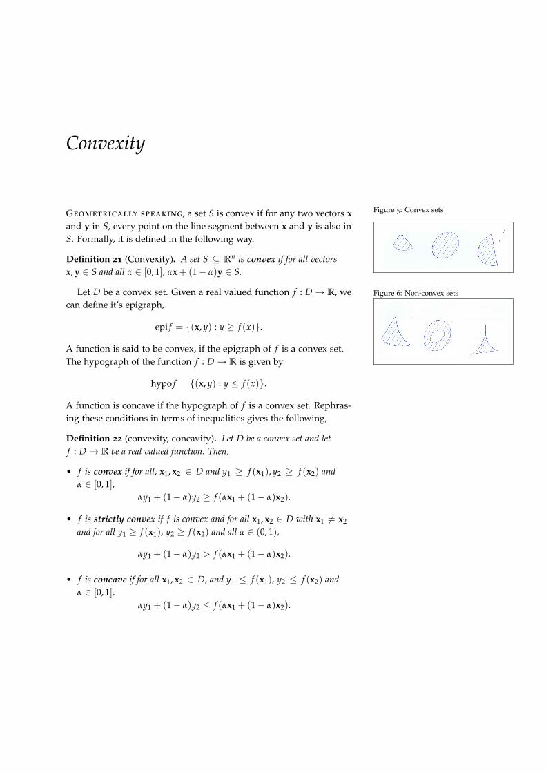
Convexity

Geometrically speaking, a set S is convex if for any two vectors xand y in S, every point on the line segment between x and y is also inS. Formally, it is defined in the following way.

Definition 21 (Convexity). A set S ⊆ Rn is convex if for all vectorsx, y ∈ S and all α ∈ [0, 1], αx + (1− α)y ∈ S.

Figure 5: Convex sets

Figure 6: Non-convex setsLet D be a convex set. Given a real valued function f : D → R, wecan define it’s epigraph,

epi f = {(x, y) : y ≥ f (x)}.

A function is said to be convex, if the epigraph of f is a convex set.The hypograph of the function f : D → R is given by

hypo f = {(x, y) : y ≤ f (x)}.

A function is concave if the hypograph of f is a convex set. Rephras-ing these conditions in terms of inequalities gives the following,

Definition 22 (convexity, concavity). Let D be a convex set and letf : D → R be a real valued function. Then,

• f is convex if for all, x1, x2 ∈ D and y1 ≥ f (x1), y2 ≥ f (x2) andα ∈ [0, 1],

αy1 + (1− α)y2 ≥ f (αx1 + (1− α)x2).

• f is strictly convex if f is convex and for all x1, x2 ∈ D with x1 ̸= x2

and for all y1 ≥ f (x1), y2 ≥ f (x2) and all α ∈ (0, 1),

αy1 + (1− α)y2 > f (αx1 + (1− α)x2).

• f is concave if for all x1, x2 ∈ D, and y1 ≤ f (x1), y2 ≤ f (x2) andα ∈ [0, 1],

αy1 + (1− α)y2 ≤ f (αx1 + (1− α)x2).

62

• f is strictly concave if f is concave and in addition for all x1, x2 ∈ Dwith x1 ̸= x2 and y1 ≤ f (x1), y2 ≤ f (x2) and all α ∈ (0, 1),

αy1 + (1− α)y2 < f (αx1 + (1− α)x2).

For D a convex set, let f : D → R be a real valued function. Defineit’s lower level set,

L fα = {x ∈ D : f (x) ≤ α}.

A function is quasi-convex if for all α, the sets L fα are convex. Theupper level set of a function f is given by,

U fα = {x ∈ D : f (x) ≥ α}.

A function is quasi-concave if for all α, the upper level sets U fα areconvex.

Definition 23 (quasi-convexity, quasi-concavity). Let D be a convex setand let f : D → R be a real valued function. Then,

• f is quasi-convex if for all x1, x2 ∈ D, and y ≥ f (x1), f (x2) andα ∈ [0, 1],

f (αx1 + (1− α)x2) ≤ y.

• f is strictly quasi-convex if f is quasi-convex and in addition for allx1, x2 ∈ D with x1 ̸= x2 and all y ≥ f (x1), f (x2) and all α ∈ (0, 1),

f (αx1 + (1− α)x2) < y.

• f : S → R is quasi-concave if for all x1, x2 ∈ D and y ≤ f (x1), f (x2)

and all α ∈ [0, 1],f (αx1 + (1− α)x2) ≥ y.

• f is strictly quasi-concave if f is quasi-concave and in addition for allx1, x2 ∈ D with x1 ̸= x2 and all y ≥ f (x1), f (x2) and all α ∈ (0, 1),

f (αx1 + (1− α)x2) > y.

Quasi-concavity or quasi-convexity is a weaker notion than convex-ity or concavity.

Lemma 4. If f is convex, then f is quasi-convex. If f is strictly convex, thenf is strictly quasi-convex. If f is concave, then f is quasi-concave and if f isstrictly concave, then f is also strictly quasi-concave.

Proof. Here we only show that convexity implies quasi-convexity.88 88 Show the other implications yourself.

Let f be convex and let f (x1), f (x2) ≤ y. Then y ≥ f (x1) andy ≥ f (x2) so by convexity,

αy + (1− α)y = y ≥ f (αx1 + (1− α)x2),

as was to be shown. The strict and concave versions follows immedi-ately.

63

Definition 24 (Convex valued correspondence). A correspondenceG : S ↠ T is convex valued if for all x ∈ S, G(x) is a convex set.

The following theorem imposed additional assumptions on Berge’stheorem in order to guarantee that the correspondence Γ(θ) is afunction. First, we need that the correspondence is convex valued.Second, it assumes that the objective function f is strictly quasi-concave.

Theorem 18. Let, X and T be two convex sets, let f : X × T → R be acontinuous function and let G : T ↠ X be a continuous, correspondence.Let,

v(θ) = maxx∈G(θ)

f (x, θ),

Γ(θ) = {x ∈ S : f (x, θ) = v(θ)}.

If f (x, θ) is quasi-concave in x and G is convex valued, then Γ is alsoconvex valued. If in addition f is strictly quasi-concave, then Γ is singlevalued.89. 89 In particular, a continuous function

Proof. Let f be concave in x and let G be convex valued. We need toshow that Γ(θ) is a convex set for all θ. If x1, x2 ∈ Γ(θ) then we havethat,

f (x1, θ) = v(θ) = f (x2, θ).

As such,

f (αx1 + (1− α)x2, θ) ≥ v(θ).

Also, as G(θ) is convex, αx1 + (1− α)x2 ∈ G(θ). So αx1 + (1− α)x1 ∈Γ(θ) as was to be shown.

For the second part, if x1 ̸= x2 then,

f (αx1 + (1− α)x2, θ) > v(θ).

However, this is impossible as v(θ) is the optimal value function. Assuch, it must be that x1 = x2 and therefore Γ(θ) must be unique.

The correspondence Γ(θ) is upper hemi-continuous, so if it is sin-gle valued, we have by Exercise 1 of the chapter on Corresondencesthat it coincides with the graph of a continuous function.

Exercises

1. Show that a function f is (strictly) convex if and only if − f is(strictly) concave.

2. Show that a function f is (strictly) quasi-convex if and only if − fis (strictly) quasi-concave.

3. Show that above theorem also holds if max is replaced by min and(strict) quasi-concave by (strict) quasi-convex.

Contraction mappings

Fixed point theorems are used in economics in order to findequilibria of various models. The two main areas of application ineconomics are general equilibrium theory and game theory. Let’sbegin by presenting the definition of a fixed point.

Definition 25. Let S ⊆ Rk be a set. A (multivariate) function f : S → Shas a fixed point at x if f (x) = x. In other words, the function f maps thefixed point x to itself.

Fixed point theory aims at imposing reasonable restrictions onthe set S or the function f such that there is at least one fixed point.We will focus on two fixed point results that are widely used ineconomics: the Banach fixed point theorem and Brouwer’s fixedpoint theorem. The first imposes rather strong restrictions on thefunction f but has the advantage that it gives an explicit procedureto find the fixed point and that the fixed point is unique. The secondimposes less restrictions on f but finding a fixed point is way moredifficult in practice. This chapter deals with the first fixed pointtheorem.

Think about how we could proceed by finding a fixed point of agiven function f . One approach would be to take an arbitrary pointx0 in S and look at its value under the mapping f , i.e. x1 = f (x0). Ifx1 = x0, we are done as x0 is then a fixed point. If x1 ̸= x0, we couldlook at the value of x2 = f (x1) and verify whether x2 = x1. We coulditerate this procedure and hopefully (at some number of iterations)end up at a fixed point.

In order to formalize this approach, define can define iterativelyxt = f (xt−1), with x0 ∈ S arbitrarily chosen and consider the se-quence (xt)t∈N. It is our hope that this sequence somehow convergestowards a fixed point in S. This will be the case, for example, if thissequence is Cauchy, i.e. terms later on in the sequence get closer andcloser together. A special class of functions for which this is generallytrue are contraction mappings.

66

Definition 26. Contraction mapping Let S ⊆ Rk. The function f : S→ Sis a contraction mapping if there is a number q ∈ [0, 1) such that for allx, y ∈ S,

∥ f (x)− f (y)∥ ≤ q∥x− y∥,

The following gives the Banach fixed point theorem better knownas the contraction mapping theorem.

Theorem 19 (Banach fixed point theorem). If f : S→ S is a contractionmapping, and S is a closed set, then f has a unique fixed point.

Proof. Let us first show that the function f is continuous. Let (xn)n∈N

be a sequence such that xn → x. We need to show that f (xn) → f (x).As f is a contraction mapping,

∥ f (x)− f (xt)∥ ≤ q∥x− xt∥.

We have that ∥x− xt∥n→ 0 so from the convergence lemma, f (xn)

n→f (x), which shows continuity of f .

Now, take any x0 ∈ S and consider the sequence (xn)n∈N, wherexn = f (xn−1) for all n ≥ 1. If this sequence has a limit x, then both(xn)n∈N and ( f (xn))n∈N converge to the same limit x ∈ S.90 As such 90 Given that (f(xn))n∈N is the sequence

(xn)n∈N shifted by one index value.f (x) = x and this limit is a fixed point. In order to show that (xt)t∈N

converges, we prove that it is a Cauchy sequence.

∀ε > 0, ∃Nε, ∀n, m ≥ N : ∥xn − xm∥ < ε.

Take two integers n, m and assume without loss of generality thatn < m, then

∥xn − xm∥ =∥∥∥∥∥m−1

∑k=n

(xk+1 − xk)

∥∥∥∥∥ ≤ m−1

∑k=n∥xk+1 − xk∥,

Also, ∥xk+1 − xk∥ = ∥ f (xk) − f (xk−1)∥ ≤ q∥xk − xk−1∥. Repeatedapplication gives,

∥xk+1 − xk∥ ≤ qk∥x1 − x0∥.

As such,

∥xt − xv∥ ≤m−1

∑k=n

qk∥x1 − x0∥,

≤ ∥x1 − x0∥∞

∑k=n

qk,

= ∥x1 − x0∥qn

1− q.

67

This last term goes to zero as n (and m) go to infinity because q < 1.As such, taking N large enough such that it is smaller than ε. This This requires that ∥x1− x0∥qN/(1− q) <

ε or

Nε >ln(

(1−q)ε∥x1−x0∥

)ln(q)

.

shows that (xn)n∈N is a Cauchy sequence.For uniqueness, assume that x and y are both fixed points of the

contraction mapping f , then it must be that,

q∥x− y∥ ≥ ∥ f (x)− f (y)∥ = ∥x− y∥.

This contradicts with the fact that q < 1 and x ̸= y.91 91 Notice that if x ̸= y then ∥x− y∥ > 0.

The Banach theorem is quite weak.92 Consider, for example, the 92 Or in other words, the restrictions onf are quite strongfunction f : [0, 1]→ [0, 1] by f (x) = x. Then | f (x)− f (y)| = |x− y| so

f is not a contraction mapping. However, every point in the domainis a fixed point.

Sometimes, the function f is not a contraction mapping but agiven iteration of f is a contraction mapping. To model this define,for a given function f : S→ S, f 2(x) = f ( f (x)), and define iterativelyf N(x) = f ( f N−1(x)).

Theorem 20. If f N : S → S is a contraction mapping for some N ∈ N,then the unique fixed point of f N is also the unique fixed point of f .

Proof. Let us first show that f has a fixed point. Let x be a fixedpoint of f N , which exists by the Contraction mapping theorem. Then,f (x) = f ( f N(x)) = f N+1(x) = f N( f (x)). This shows that f (x) isalso a fixed point of f N . Given that the fixed point of f N is unique, itmust be that f (x) = x. Another way to see this is to notice that if x isa fixed point of f N , then,

∥ f (x)− x∥ = ∥ f ( f N(x))− f N(x)∥,= ∥ f N( f (x))− f N(x)∥,≤ q∥ f (x)− x∥.

for some 0 < q < 1. However, this can only be if ∥ f (x)− x∥ = 0 whichshows that f (x) = x, or equivalently, x is a fixed point of f .

Now, let us show that the fixed point of f is unique. The proofis by contradiction. Assume that f has two fixed points x and yand x ̸= y. But then, repeatedly application of f on x and y gives,f N(x) = x and f N(y) = y contradicting the fact that f N is a contrac-tion mapping with a unique fixed point.

Theorem 21. If f : [a, b] → [a, b] is C1 and supx∈[a,b] | f ′(x)| < 1 for allx ∈ [a, b], then f is a contraction mapping.

Proof. Let x, y ∈ [a, b]. Then by the mean value theorem, there is ac ∈ [x, y] such that, f ′(c)[y− x] = f (y)− f (x), so,

| f (y)− f (x)| = | f ′(c)(y− x)| ≤ | f ′(c)||y− x|.

68

Together with | f ′(c)| ≤ supx∈[a,b]| f ′(x)| < 1, this shows that f is acontraction mapping.

Exercises

1. Show that f (x) = 1− x5 is not a contraction mapping over [0, 1]but that it does have a fixed point.

2. Let f (x) = x + e−x. Is f a contraction mapping?

3. Using the contraction theorem, prove that the following sequencesare convergent,

•√

2,√

2 +√

2,√

2 +√

2 +√

2, . . . ,

•√

3,√

3 +√

3,√

3 +√

3 +√

3, . . . ,

4. Let f : S → S be a function where S ⊆ Rn is a compact set.Assume that for all x, y ∈ S with x ̸= y,

∥ f (x)− f (y)∥ < ∥x− y∥.

Show that f has a unique fixed point.

5. Give an example of a function f that is not a contraction mappingbut satisfies the condition in the previous exercise.

Sperner’s lemma

The major fixed point theorem is due to Brouwer. There are severalproofs of Brouwer’s fixed point with various degrees of difficulty.The easiest93 relies on an intermediate result that is called Sperner’s 93 Probably.

lemma. In order to introduce this lemma, it is necessary to providesome additional notation and definitions.

A polyhedral is the convex combination of a finite number ofvectors. An n-dimensional simplex, denoted by Sn is a polyhedralwhich is the convex combination of n + 1 linearly independentvectors.94 An n dimensional simplex lies in an n dimensional plane 94 The vectors x0, . . . , xn are linearly

independent if ∑ni=0 αixi = 0 only if all

αi = 0. In two dimensional space, 3

vectors are independent if they form atriangle.

of Rn+1.

Example:• S1 is the one dimensional simplex. It is formed by the convex com-

bination of 2 linearly independent vectors. This means that S1 is aline segment.

• S2 is the 2 dimensional simplex. It is formed by the convex combi-nation of 3 linearly independent vectors, which means that S2 is atriangle.

• S3 is the 3-dimensional simplex. it is formed by the convex combi-nation of 4 linearly independent vectors, so it is a tetahedron.

For these lecture notes, we will look at S1 and S2, i.e. line seg-ments and triangles. Sperner’s lemma, however, also extends tohigher dimensions.

Consider a one dimensional simples S1, better known as a linesegment. Let us denote the left endpoint of the segment by pℓ andthe right endpoint by pr. It is fairly easy to subdivide this line seg-ment into smaller segments. This can be done by picking pointsp1, p2, . . . , pn on the line segment (pℓ, pr). Giving the smaller seg-ments,

(pℓ, p1), (p1, p2), (p3, p4), . . . , (pn, pr).

Dividing the segment into smaller segments is called a simplical

70

subdivision. The points pℓ, p1, . . . , pn, pr are called the vertices of thesubdivision.

Let us now colour these vertices. For a one dimensional simplex,we pick two colours, say red and blue and we may colour the verticesanyway we want except for the fact that pℓ and pr have differentcolours. Such colouring is called a Sperner colourling.

Figure 7: A Sperner colouring of S1

Theorem 22 (Sperner). Let S1 be a one-dimensional simplex which issubdivided. Assume that all points are coloured in one of two colours andthat pℓ and pr have different colours (i.e. a Sperner colouring). Then thereare an odd number of sub-segments for which both vertices have differentcolours.

Proof. Use the following analogy. Let the line segment be a buildingand let the points pℓ, p1, . . . , pn, pr be the walls of the building. Asubsegment (pi, pi+1) is a room in the building.95 Let’s put a door 95 This is a one-dimensional building, so

a room has only two walls.in every wall that has the color red. And before every door we put adoormat, but only when we are inside the room.96 96 In other words, we don’t put door-

mats outside the building.How many doormats are there? Well we can count the number ofdoormats in two different ways. First of all, according to the doors inour building. We have one door that goes to the ouside,97 Next, for 97 There is the door in wall pℓ or pr

according to which one of the two hasthe colour red.

every door on the inside, we have to put two doormats as each suchdoor connects two rooms. As such,

# mats = 2 (# inside doors ) + 1.

Next, let us count the number of mats according to the rooms. Thereare three kind of rooms. Rooms where both walls are red. Roomswhere both walls are blue and rooms where one wall is red andone is blue. The first type of room has 2 doormats (as there are twodoors). The second type of door has no doormats. The third type hasone doormat. As such,

# mats = 2 (# red-red room) + (# red-blue room).

Equating the two ways of counting the doormats gives,

2 (# inside doors ) + 1 = 2 (# red-red room) + (# red-blue room),

↔(# red-blue room) = 2 ((# inside doors )− (# red-red room)) + 1.

The right hand side is an even number plus an odd number, so it isodd. This means that the number of red-blue rooms should also beodd, in particular, there should be at least one.

Let us now have a look at the two dimensional simplex S2, whichis a triangle. First, we need to divide the triangle into smaller trian-gles. There are many ways to do this but the following will work.Take a triangle,

71

pbpa

pc

divide each side of the triangle in half and connect these points. Thisgives four smaller triangles.

pbpa

pc

Each side of this smaller triangle can again be divided in foursmaller ones.

pbpa

pc

72

and so on . . . .Each time we get smaller and smaller triangles. Let pa, pb and

pc be the three vertices of the big triangle and let p1, p2, . . . pn be allother vertices in the triangulation. We will denote the big triangle byT and the small triangles by T1, T2, . . . , Tm. We will colour the verticesin 3 colours. The rules are the following

• The three vertices of the big triangle pa, pb, pc have differentcolours.

• If a vertex pi is on one of the sides of the big triangle, it needs tohave the colour of one of the vertices of the big triangle that makesthis side. For example if pi is on the line segment made up by pa

and pb then pi must have the colour of pa or the colour of pb.

Such colouring is called a Sperner colouring.

Figure 8: Sperner colouring of S2

Theorem 23. Consider a triangulation of which the vertices are colouredaccording to the rules above, i.e. a Sperner colouring. Then there are an oddnumber of small triangles Ti of which the three vertices that make up thesetriangles all have distinct colours.

Proof. Let the colors be red, blue and green. Assume, wlog that pa isred, pb blue and pc green.

We will, once more, use the building analogy. Let the big trianglebe our building. A room is now a small triangle and (obviously)every room now has three walls, where each wall is defined by twovertices of the small triangle. These vertices which may or may nothave different colours, so every wall is defined by two (possiblyidentical) colours.

Pick two of the three colours, say red and blue and let us put adoor into every wall with these colours. Finally, we put a doormat infront of all doors, but only on the inside of the building.

As in the previous Theorem, we will count the number of door-mats in two different ways, according to the number of doors andonce according to the number of rooms.

Concerning the second option, there are three types of rooms.Rooms with the colours red-blue-green have one single door (in thered-blue wall). Rooms with colours red-red-blue and red-blue-bluehave two doors as there are two red-blue walls. Therefore, they alsohave two doormats. Finally, rooms with colours red-red-green; red-green-green; blue-blue-green or blue-green-green have no doors, sono doormats. Given this, the total number of doormats is given by

# mats =# red-blue-geen rooms,

+ 2 # red-blue-blue rooms,

+ 2 # red-red-blue rooms.

73

Next, let us count the doormats according to the number of doors.First, let us look at the outside of the building. There are no doorson the (pa, pc) nor (pb, pc) segments as these vertices only have thecolours red-green or green-blue.

As such, all doors are on the line segment going from pa to pb.All walls on this segment have vertices that are coloured with red orblue. As such, by the previous Theorem, there are an odd numberof (walls) line segments with distinct colours which are exactly thewalls with the doors. As such, there are an odd number of doors onthe outside of the big triangle. Each of these doors have exactly onedoormat.

Next, for every door on the inside of the triangle, these doorsconnect two rooms. So there are two doormats for each inside door.As such,

# mats =# doors on boundary of big triangle,

+ 2 # doors in interior.

Equating the two equations gives,

# red-blue-geen rooms =2 # doors in interior,

− 2 # red-blue-blue rooms,

− 2 # red-red-blue rooms,

+ # doors on boundary of big triangle.

The right hand side of this equation is odd, so the left hand sideshould also be odd. In particular, there is at least one room withthree distinct colours.

Exercises

1. Prove the following grid version of Sperner’s lemma: Consider a3-coloring over {0, 1, . . . , n} × {0, 1, . . . , n}. The coloring is proper if

• The color of (0, i) is ‘red’ for all i ∈ {0, 1, . . . , n}.

• The color of (i, 0) is ‘green’ for all i ∈ {1, . . . , n}. and

• All other points on the boundary of the grid are blue.

Show that any proper 3-coloring has a unit-size square whosevertices have all three colors.

Brouwer’s fixed point theorem

The Brouwer fixed point theorem is one of the most fascinating and important theorems of 20th century mathe-matics. Proving this theorem established Brouwer as one of the preeminent topologists of his day. But he refusedto lecture on the subject, and in fact he ultimately rejected this (his own!) work. The reason for this strangebehavior is that Brouwer had become a convert to constructivism or intuitionism. He rejected the Aristoteliandialectic that a statement is either true or false and there is no alternative, so he rejected the concept of “proof bycontradiction”.

(Stefen G. Krantz in the history of Mathematics, edited by Lundsgaard and Gray)

The major fixed point theorem is due to Brouwer.

Theorem 24 (Brouwer). If S is compact and convex and f : S → S iscontinuous then f has a fixed point in S.

We will first proof the theorem for a particular kind of convexcompact set, namely the n− 1-dimnesional unit simplex. It is given by,

∆n−1 =

{x ∈ Rn

+ :n

∑j=1

xj = 1

}.

The set ∆n−1 consists of all non-negative n-dimensional vectors

whose components sum to one. For ∆1 these are the vectors x =

[x1

x2

]such that x1, x2 ≥ 0 and x1 + x2 = 1. In other words, the vectors on

the line segment connecting

[10

]with the point

[01

]. Notice that this

is simply a one-dimensional object, namely a line segment. As such,we can see this as being a one-dimensional simplex.

Figure 9: The one dimensional unitsimplex

0

1

1

The two dimensional unit simplex ∆2 consists of the three dimen-

sional vectors x =

x1

x2

x3

such that x1, x2, x3 ≥ 0 and x1 + x2 + x3 = 1.

These are the vectors that lie in the triangle bounded by the corners100

,

010

and

001

.

Figure 10: The two dimensional unitsimplex

1

1

1

It is simply a triangle, so a 2 dimensional simplex.

76

The following theorem shows that any continuous function from∆n to itself has a fixed point.

Theorem 25. Let f : ∆n → ∆n be a continuous function. Then there is anx ∈ ∆n such that f (x) = x.

Proof. We will prove it for the two dimensional simplex ∆2. Re-member, ∆2 consists of 3-dimensional non-negative vectors whosecomponents add up to one. The proof uses Sperner’s lemma from theprevious chapter.

Consider ∆2, the two dimensional unit simplex. Let f : ∆2 → ∆2

be a continuous function. We will show that f has a fixed point. Theproof is by contradiction, so assume that f (x) ̸= x for all x ∈ ∆2.

Consider a triangulation ∆2 into small triangles. We will colourthe vertices of this triangulation in the following way. Consider

three colours, red, blue and green. Let v =

v1

v2

v3

be a vertex of the

triangulation.98 98 Remember points in ∆2 are 3-dimensional non-negative vectorswhose components add up to one.

Then we can put,

f (v) =

f1(v)f2(v)f3(v)

we know that f (v) ∈ ∆2 so, f1(v), f2(v), f3(v) ≥ 0 and f1(v) + f2(v) +f3(v) = 1. We give v the following colour,

f1(v)) < v1 → red,

f1(v) ≥ v1 and f2(v) < v2 → blue,

f1(v) ≥ v1 and f2(v) ≥ v2 and f3(v) < v3 → green.

First of all, let us show that we can actually colour each vertex. If not,it must be that f1(v)) ≥ v1, f2(v) ≥ v2 and f3(v) ≥ v3. However, asv1 + v2 + v3 = 1 = f1(v) + f2(v) + f3(v), we have that fi(v) = vi

for i = 1, 2, 3 so f (v) = v or equivalently, v is a fixed point, acontradiction.99 99 Show this, i.e. if ∑n

i=1 xi = ∑ni=1 yi and

xi ≤ yi for all i then xi = yi for all i.Next, let us show that the colouring is in fact a Sperner colouring.

First we need that xa =

100

is red, xb =

010

is blue and xc =

001

is green.100 Next, for any vector on the line segment xa and xb is 100 Show this.

either red or blue. Well every vector on this segment has a zero forthe third component, so it can not have the colour green. As such, itmust be either red or blue as desired. Similarly, we can show that anyvector on the segment (xb, xc) is blue or green and any vector on thesegment (xa, xc) is red or green.

77

Given this Sperner colouring, we know that there must be a smalltriangle with three different colours. Let Ti be this small triangle andlet y, z, w be the vectors of this triangle with colours, red, blue, greenrespectively. We know that y1 > f1(y), z2 > f2(z) and w3 > f3(w).

The idea is to take a sequence of finer and finer triangulations.Each time, we can find a smaller and smaller triangle with threedifferent colours and vertices y in red, z in blue and w in green. Thiscreates a sequence of vectors,

(yn)∞n=1, (zn)

∞n=1, (wn)

∞n=1.

Where the vectors yn, zn, wn get closer and closer together as n→ ∞.Now, given that the space ∆2 is compact, we can find subse-

quences that converge,101 101 First take a subsequence along ynconverges. Then from this subsequence,take a further subsequence along whichzn also converges and from this sub-subsequence, take a subsequence alongalso wn converges.

yφ(n) → y, zφ(n) → z, wφ(n) → w.

Of course, given that the distances between these vectors yφ(n), zφ(n), wφ(n)become smaller and smaller, it must be that y = z = w, i.e. the subse-quences converge to the same vector. Also, for all n,

f1(yφ(n)) < yφ(n),1,

f2(zφ(n)) < zφ(n),2,

f3(wφ(n)) < wφ(n),3.

Now, taking the limit for φ(n) → ∞ from both left and right handside, and given continuity of f , we get,

f1(y) ≤ y1,

f2(y) ≤ y2,

f3(y) ≤ y3.

Also y ∈ ∆2 so y1 + y2 + y3 = f1(y) + f2(y) + f3(y) which gives thatf (y) = y or equivalently, y is a fixed point. This gives the desiredcontradiction.

Now, let’s go back to Brouwer’s theorem: if f : S → S is contin-uous and S is a compact and convex set, then f has a fixed point.We have shown that the theorem is true for S = ∆n, so how can wegeneralize this result for all S, compact and convex. We we can usethe following lemma.

Theorem 26. Let T be a compact set in Rn such that there is a one to onecontinuous function g : T → ∆n. If f : T → T is continuous, then f has afixed point.

78

Proof. Consider the mapping h : ∆n → ∆n where h(x) = g( f (g−1(x))).So it takes a point x from ∆n maps it to T via g−1. Then maps it ac-cording to f and transfers it back to ∆n via g.

The function h is a continuous map from S to S as it is the compo-sition of continuous functions. Also, by the previous theorem h has afixed point in ∆n, i.e. a vector x ∈ ∆n such that h(x) = x. But then,

g( f (g−1(x))) = x,

⇐⇒ f (g−1(x)) = g−1(x).

As such, g−1(x) ∈ T is a fixed point of f .

Given this result, the only thing we need to show is that if S isconvex and compact then there exists a one-to-one and continuousfunction g : S→ ∆n. Luckily this is the case,102 102 I skip the proof of this result.

Lemma 5. If S ⊆ Rk is convex and compact then there is a m ≤ k and a oneto one continuous function g : S→ ∆m.

Exercises

1. Let f (x) = x2 and suppose that S =]0, 1[. Show that f has no fixedpoint even though it is a continuous mapping from S to S. Doesthis contradict Brouwer’s theorem, why, why not?

2. Use Brouwer’s theorem to show that the equation cos(x)− x −1/2 = 0 has a solution in the interval 0 ≤ x ≤ π

4 .

3. Place a map of your country on the floor. Show that there is atleast one point on the map that is exactly above the point it isreferring to.

General equilibrium in exchange economies

When Debreu received his Nobel prize in 1983, he was accosted by journalists who wanted to know his viewsabout where the economy was headed. He is said to have thought awhile and then continued, “Imagine aneconomy with n goods and m consumers. . . ”

A sizeable part of economics looks at the optimal behaviour of con-sumers and producers buying and selling goods. These consumersand producers meet each other on markets. The transaction of goodsis governed by (relative) prices. And as equilibrium dictates, pricesshould be set as to equalize demand and supply.

As economists we are find it obvious that there should be someprices at which markets clear. However, if you think more carefullyabout this, there is something peculiar going on. Prices for certaingoods, will affect the demand and supply for other goods and there-fore their prices. These price adjustments in turn affect demand andsupply behaviour on other markets and therefore the prices of othergoods. Given this, it is not at all obvious that there should exist asingle price vector that equates the supply and demand for all goodssimultaneously. The fact that such equilibrium price vector exists,is one of the main theoretical results of economic theory of the pastcentury. Its proof relies heavily on Brouwer’s fixed point theorem. The proof is due to Lionel McKenzy,

Kenneth Arrow and Gérard Debreu.

Consider an economy with N consumers. Each consumer hasan endowment of goods. We denote the endowment of consumer iby ei ∈ Rk

+. The endowment is simply a vector of good quantities,ei

j is the amount of good j that consumer i has to start with. Each

consumer also has a utility function ui : Rk → R where ui(q) givesthe utility of consumer i for consuming the bundle q ∈ Rk

+. Theeconomy can be represented by the tuple

E = {N, (ui, ei)i≤N}.

We consider the case of an exchange economy. This means thatthere is no production (firms) involved. However, consumers areallowed to trade with each other.

We require that that the utility functions ui are continuous and

80

strictly quasi-concave. We also assume that goods are traded (i.e.bought and sold) according to some price vector p ∈ Rk

++. If everyconsumer is price taker, then the budget constraint of consumer i (i.e.the goods that she can consume) is given by,

Bi(p) = {q ∈ Rk+ : p · q ≤ p · ei}.

It can be shown that this correspondence Bi(p) is continuous on Rk++.

As such,

maxq∈Bi(q)

ui(q),

leads, by Berge’s theorem, to an optimal solution, say di : Rk++ → Rk,

which gives the optimal consumption bundle of consumer i, di(p)for a given price vector p. We know this function continuous forp ∈ Rk

++.In addition to continuity and strict quasi-concavity, we also as-

sume that utility functions are locally non-satiated.

Definition 27 (locally non-satiation). The function ui : Rk+ → R is locally

non-satiated if for all x ∈ Rk+ and all ε > 0 there is a y ∈ Rk

+ such that,

∥x− y∥ < ε and ui(y) > ui(x).

Local non-satiation states that at any bundle there is always an-other bundle arbitrarily close that gives a higher utility.

The following result shows that if utility functions are locallynon-satiated, then the budget constraint will be binding.

Lemma 6. If ui is locally non-satiated then p · di(p) = p · ei.

Proof. Let x = di(p). We know that p · x ≤ p · ei. Towards a contra-diction, assume that p · x < p · ei. Let ε = p · ei − p · x > 0. Then for∥y− x∥ < ε/∥p∥, we have that,103 103 Observe the use of the Cauchy-

Schwartz inequality.p · y = p · x + p · (y− x),

= p · ei − ε + p · (y− x),

≤ p · ei − ε + ∥p∥∥y− x∥,< p · ei.

As such there is a δ > 0 such that for all y ∈ Rk with ∥y− x∥ < δ,p · y ≤ p · ei.104 Also, by locally non-satiation there should be at least 104 Set δ = ε/a.

one such y for which ui(y) > ui(x), a contradiction with optimalityof x.

Let di(p) be the demand function of consumer i at prices p. Inaddition, consumer i has an endowment ei. The excess demandfunction of consumer i is defined as,

di(p)− ei.

81

If for goods j, dij(p)− ei

j > 0, then the consumer will buy this good

on the market. If on the other hand, good j has dij(p)− ei

j < 0, thenthe consumer will sell this good on the market. If we sum the excessdemand functions of all consumers together, we obtain the so calledaggregate excess demand function.

Definition 28 (Aggregate excess demand function). The (aggregate)excess demand function is defined as,

z(p) =N

∑i=1

(di(p)− ei)

The following gives some properties of the excess demand func-tion.

Lemma 7. If z(p) : Rk++ → Rk is an excess demand function then,

• p · z(p) = 0.

• for all λ > 0, z(λp) = z(p).

• z : Rk++ → Rk is continuous.

Proof. We have that,

p · z(p) =N

∑i=1

(p · di(p)− p · ei

),

= 0,

by the fact that every consumers budget is balanced. Homogeneityfollows from the fact that di(λp) = di(p). Rescaling of the pricesdoes not change the budget constraint so it does not influence theoptimization problem. Finally z is continuous as it is the sum ofcontinuous functions.

The first property p · z(p) = 0 is called Walras’ law. It holds forevery price vector and is a simple consequence from the fact that allconsumers have a balanced budget.

The homogeneity of degree zero property, i.e. z(λp) = z(p) allowsus to focus on price vectors p ∈ Rk

++ for which ∑i pi = 1.105 This 105 Set λ = 1∑i pi

.

allows us to define the domain of the excess demand function to bethe k− 1 dimensional simplex. So we can set z : ∆k−1 → Rk.

We say that the price vector p is an equilibrium price if demand isequal to supply on all markets. In other words, the excess demandfunction is zero.106 106 Or the excess demand can be nega-

tive if prices are zero. These are thengoods that nobody really wants.Definition 29. Let z(p) be an excess demand function. Then p∗ is an

equilibrium price vector ifz(p∗) ≤ 0.

and if zj(p∗) < 0, then pj = 0.

82

Theorem 27. Let z : ∆k−1 → Rk be a continuous function that satisfiesWalras’ law (p · z(p) = 0 for all p ∈ ∆k−1). Then there exists an equilibriumprice vector.

Proof. Consider an auctioneer whose task is to produce an equilib-rium on all markets. What will this auctioneer do. Well she willincrease the prices of the goods whose excess demand is strictlypositive.107 107 And lower the price of the goods if

the excess demand is negative.Letgj(p) = max{0, zj(p)}.

If gj(p) > 0 then demand is greater than supply, so the price of goodj should go up. Say the updated price evolves according to

pj + gj(p).

Of course, the auctioneer should also make sure that the pricesremain in the simplex ∆k−1. This can be done by dividing this “newprice” by the sum of all “new prices”, giving the updated price ofgood j by,108 108 Notice that ∑j pj = 1.

pj + gj(p)

1 + ∑kt=1 gt(p)

.

Define the function f : ∆k−1 → ∆k−1 by,109 109 Check that f j(p) ≥ 0 and ∑j f j(p) =1.

f j(p) =pj + gj(p)

1 + ∑kt=1 gt(p)

.

Also f j(p) is continuous.110 By Brouwer’s fixed point, f should have 110 This follows from the fact that gj(p)is continuous.a fixed point, say p∗. Then, for all goods j,

p∗j =p∗j + gj(p∗)

1 + ∑kt=1 gt(p∗)

,

↔pj

k

∑t=1

gt(p∗) = gj(p∗).

Let us multiply each side of this equality by zj(p∗) and sum over allgoods j. (

k

∑t=1

gt(p∗)

)(k

∑j=1

pjzj(p∗)

)=

k

∑j=1

zj(p∗)gj(p∗).

The left hand side is equal to zero by Walras’ law (p · z(p)) = 0. Assuch,

k

∑j=1

zj(p∗)gj(p∗) =k

∑j=1

zj(p∗)max{0, zj(p∗)} = 0.

If for good j, zj(p∗) ≤ 0 then the corresponding term is zero.111 On 111 As gj(p∗) = 0, we have thatzj(p∗)gj(p∗) = 0.

83

the other hand if zj(p∗) > 0 then the term is strictly positive.112 As112 As gj(p∗) > 0.such, this is a sum of non-negative numbers that should add up to

zero. Conclude that all terms should equal zero, or equivalently, forall goods j, zj(p∗) ≤ 0.

Now, if for some good j, zj(p∗) < 0 then as p∗ · z(p∗) = 0 it mustbe that p∗j = 0, which shows the second part.

A careful reader may have noticed that in Theorem 27 we assumedcontinuity of z(p) for all price vectors in ∆k−1. This includes the pricevectors which have zero components. On the other hand, in Lemma7 we demonstrated continuity of z(p) for all price vectors whosecomponents are strictly positive, i.e. p≫ 0. We could only proof con-tinuity for p ≫ 0 because our assumptions are not strong enough toensure that individual demand functions di(p) are continuous whenthe prices for some goods are equal to zero.113 It is possible to ac- 113 If prices of a good is zero, it might

be that the demand of this good goes toinfinity.

count for this discrepancy at the cost of introducing some additionalassumptions but this makes the proof considerably more complicated.I refer to the handbook of Jehle and Reny (Advanced MicroeconomicTheory, 2011) for the fine details.

Kakutani’s fixed point theorem

Shizuo Kakutani was a Japanese mathematician. At the start of World War II, he was a visiting professor at theInstitute for Advanced Study in Princeton. With the outbreak of war he was given the option of staying at theInstitute or returning to Japan. He chose to return because he was concerned about his mother. So he was put ona Swedish ship which sailed across the Atlantic, down around the Cape, and up to Madagascar, or thereabouts,where he and other Japanese were traded for Americans aboard a ship from Japan. The trip across the Atlanticwas long and hard. There was the constant fear of being torpedoed by the Germans. What, you may wonder, didKakutani do. He proved theorems. Every day, he sat on deck and worked on his mathematics. Every night, hetook his latest theorem, put it in a bottle and threw it overboard. Each one contained the instruction that if foundit should be sent to the Institute in Princeton. To this day, not a single letter has been received.

Stanley Eigen, Annals of Improbable Research

Brouwer’s fixed point theorem is very powerful. Sometimes,however we would like to have a fixed point for correspondencesand not just functions. Remember, a function associates with eachpoint in a domain a unique point in the range. A correspondence, onthe other hand, can correspond to any point in the domain, multiplepoints in the range.

Definition 30. Let G : S ↠ S be a correspondence. The vector x ∈ S is afixed point of G if x ∈ G(x).

Figure 11 gives a correspondence with a fixed point: 1/2 ∈ G(1/2).This case, however, can not be handled by the Brouwer fixed pointtheorem as the correspondence is not a function.

Figure 11: A correspondence with afixed point.

0 1

1

The following gives the main fixed point results for correspon-dences, known as Kakutani’s fixed point theorem.

Theorem 28 (Kakutani). Let G : S ↠ S be a upper hemicontinuousconvex valued correspondence on a compact and convex set S, then there isan x ∈ S such that x ∈ G(x).

Proof. (sketch) The idea is to use Brouwer’s fixed point after approxi-mating the correspondence with a function. The problem is that theredoes not necessarily exist a continuous function f : S → S such thatf (x) ∈ G(x) for all x ∈ S. If such a function existed we could pick thefixed point of f , which would give x = f (x) ∈ G(x), so we’d have afixed point of G.

86

The idea is to slightly expand the graph of G by a small amount.In particular define the ε-ball around the graph of G,

Bε(grG) ={(x, y) ∈ S× S|∃(x′, y′), y′ ∈ G(x′),

∥∥(x, y)− (x′, y′)∥∥ < ε

}.

Define the correspondence Gε where y ∈ Gε(x) if (x, y) ∈ Bε(grG).If the graph G is closed and convex, then for any ε > 0, there existsis a continuous function fε such that for all x, fε(x) ∈ Gε(x) (This iswhere the convexity part kicks in; this result is called von Neumann’sapproximation theorem.114 By Brouwer’s theorem, fε has a fixed 114 We are skipping the proof.

point.In this way, we can find a sequence of continuous functions

( f1/n)n∈N0 , such that f1/n(x) ∈ G1/n(x) for all x ∈ S. Each of thesefunctions has a fixed point, say x̂n. Also, because of the way that theset Bε(grG) is defined, we know that for all n there are (xn, yn) withyn ∈ G(xn) such that ∥(x̂n, x̂n)− (xn, yn)∥ < 1/n.

As S is compact, the sequence (x̂n)n∈N has a convergent subse-quence, say (x̂φ(n))n∈N with xφ(n)

n→ x̂. But then (xφ(n), yφ(n))n→

(x̂, x̂). As G is upper hemicontinuous, it follows that (x̂, x̂) is in thegraph of G, so x̂ ∈ G(x̂) which gives us the fixed point.

Exercises

1. Let C be a correspondence from [0, 2] into itself defined as

C(x) =

{{1}, if 0 ≤ x < 1,[0, 2] if 1 ≤ x ≤ 2

Show that C satisfies all the conditions of Kakutani’s theorem.

2. Verify whether the Kakutani fixed point theorem holds for thefollowing correspondences from the unit interval [0, 1] to itself. Foreach correspondence, explain which conditions hold and fail, andidentify the set of fixed points.

• G(x) = {y ∈ X|∥y− x∥ ≤ 1/5}.

• H(x) = {y ∈ X|∥y− x∥ ≥ 1/10}.

• L(x) = arg maxy ∥y− x∥

• M(x) = co(L(x)).

Existence Nash equilibrium

(Recommendation letter by Richard Duffin, Nash’s undergraduate advisor at the Carnegie Institute ofTechnology, to Solomon Lefschetz, a math professor at Princeton)

In this last chapter, we will use Kakutani’s fixed point theoremto show a second great theoretical result in economics, namely theexistence of a Nash equilibrium.

A normal form game is given by a tuple (N, ui, Ai). Here, N isa finite set of players and Ai ⊆ Rk is the set of actions of player i.The sets Ai are assumed to be compact and convex. The functionsui : ∏i Ai → R is the utility or payoff function of player i ∈ N. Eachfunction ui is assumed to be continuous and quasi-concave in ownactions.

Let us restrict ourselves to a situation with only two players, 1 and2.115 The Nash equilibrium assumes that each player chooses her 115 The proof can easily be extended to

more than two players at the cost ofmore confusing notation.

best action give the action chosen by the other player. This gives the

88

following optimal value and best response correspondences,

v1(a2) = maxa1∈A1

u1(a1, a2),

B1(a2) = {a1 ∈ A1 : u1(a1, a2) = v1(a2)},v2(a1) = max

a2∈A2u2(a1, a2),

B2(a1) = {a2 ∈ A2 : u2(a1, a2) = v2(a1)}.

By assumption, the sets A1, A2 are compact and convex and theutility functions are continuous and quasi-concave. Given this, weknow that the problems are well defined and in particular B1(a1) andB2(a2) are upper hemicontinuous and convex valued.

A strategy profile is a Nash equilibrium if it is a best response forall players simultaneously.

Definition 31. A strategy profile (a1, a2) is a Nash equilibrium if a1 ∈B1(a2) and a2 ∈ B2(a1).

The idea is to reformulate the property of a Nash equilibrium asthe fixed point of a correspondence. We do this in the following way.Let

B(a1, a2) = {(b1, b2) ∈ A1 × A2 : b1 ∈ B(a2), b2 ∈ B(a1)}.

This is a correspondence from A1 × A2 to A1 × A2. We have that(b1, b2) ∈ B(a1, a2) if b1 is a best response of player 1 to a2 and if b2

is a best response of player 2 to a1.The crucial property of this correspondence is that (a1, a2) ∈

B(a1, a2) if and only if (a1, a2) is a Nash equilibrium. In other words,the Nash equilibria are the fixed points of the correspondence B.

Theorem 29. Every normal form game has a Nash equilibrium.

Proof. It is easy to check that B : A1 × A2 ↠ A1 × A2 is upperhemicontinuous and convex valued.116 116 This follows from the fact that both

B1 and B2 are upper hemicontinuousand convex valued.

Also A1 × A2 is convex and compact. As such, if we apply Kaku-tani’s fixed point theorem, we find that there is a strategy pair(a1, a2) ∈ B(a1, a2), i.e. a Nash equilibrium.

Exercises

1. Consider two firms in a Cournot duopoly. Assume that q1 andq2 are the output levels of firm 1 and 2 respectively. The inversedemand function is given by P(q1 + q2).117 Assume that both firms 117 The function P(q) gives the price

at which the consumer demands anamount q.

have cost functions given by c1(q1) and c2(q2). What conditionsguarantee that there exists a Nash equilibrium?

89

2. Consider a two player game where each player has a finite num-ber of pure strategies. Consider the mixed extension where eachplayer can choose a probability distribution over her pure strate-gies. Use above theorem to show the existence of a mixed strategyNash equilibrium.