MATH32062 Algebraic Geometry

1 Affine algebraic varieties

1.1 Definition of affine algebraic varieties

We want to define an algebraic variety as the solution set of a collection ofpolynomial equations, or equivalently, a set where every element of a set ofpolynomials vanishes. Then every combination of those polynomials vanishes onthe set, so we can use the ideal generated by those polynomials to define thealgebraic variety. This motivates the definition below. Using ideals instead ofconcrete polynomials also turns out to be more useful for proving most of thetheorems about algebraic varieties.

In the following, K denotes an arbitrary field, unless specified otherwise.

Definition. An affine algebraic variety is a set of the form

V(I) = {(a1, a2, . . . , an) ∈ Kn | f(a1, a2, . . . , an) = 0,∀f ∈ I},

where I is an ideal I / K[x1, x2, . . . , xn].

It is clear from the definition that if I1 ⊆ I2, then V(I1) ⊇ V(I2), but I1 $ I2does not imply V(I1) % V(I2), see examples 7 and 8 below. Conversely, V(I1) %V(I2) does not imply I1 $ I2. (Try to think of an example where I1 6⊂ I2, butV(I1) ⊃ V(I2).)

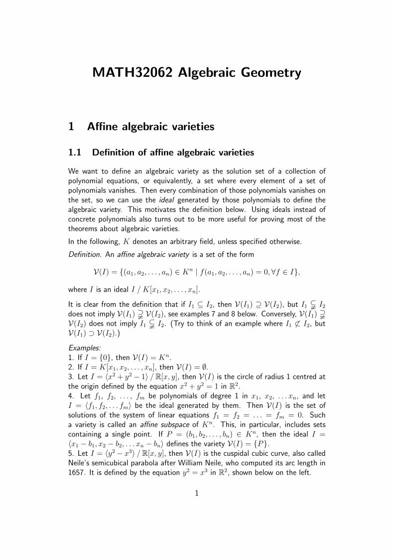
Examples:1. If I = {0}, then V(I) = Kn.2. If I = K[x1, x2, . . . , xn], then V(I) = ∅.3. Let I = 〈x2 + y2 − 1〉 /R[x, y], then V(I) is the circle of radius 1 centred atthe origin defined by the equation x2 + y2 = 1 in R2.4. Let f1, f2, . . . , fm be polynomials of degree 1 in x1, x2, . . .xn, and letI = 〈f1, f2, . . . fm〉 be the ideal generated by them. Then V(I) is the set ofsolutions of the system of linear equations f1 = f2 = . . . = fm = 0. Sucha variety is called an affine subspace of Kn. This, in particular, includes setscontaining a single point. If P = (b1, b2, . . . , bn) ∈ Kn, then the ideal I =〈x1 − b1, x2 − b2, . . . xn − bn〉 defines the variety V(I) = {P}.5. Let I = 〈y2 − x3〉 /R[x, y], then V(I) is the cuspidal cubic curve, also calledNeile’s semicubical parabola after William Neile, who computed its arc length in1657. It is defined by the equation y2 = x3 in R2, shown below on the left.

1

-0.5 0.5 1.0 1.5 2.0 2.5

-4

-2

2

4

-1 1 2

-4

-2

2

4

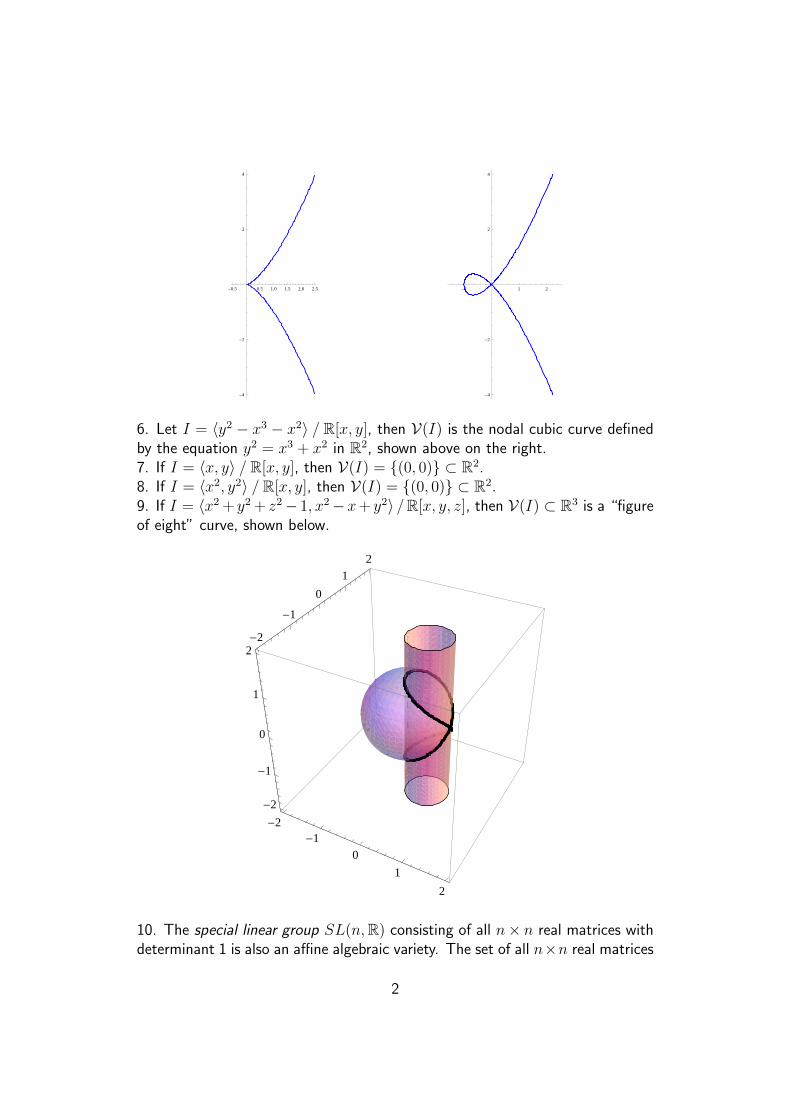
6. Let I = 〈y2 − x3 − x2〉 / R[x, y], then V(I) is the nodal cubic curve definedby the equation y2 = x3 + x2 in R2, shown above on the right.7. If I = 〈x, y〉 / R[x, y], then V(I) = {(0, 0)} ⊂ R2.8. If I = 〈x2, y2〉 / R[x, y], then V(I) = {(0, 0)} ⊂ R2.9. If I = 〈x2 + y2 + z2− 1, x2−x+ y2〉 /R[x, y, z], then V(I) ⊂ R3 is a “figureof eight” curve, shown below.

-2-1

0

1

2

-2

-1

0

12

-2

-1

0

1

2

10. The special linear group SL(n,R) consisting of all n× n real matrices withdeterminant 1 is also an affine algebraic variety. The set of all n×n real matrices

2

is Rn2, the determinant is a polynomial in the entries of the matrix, therefore

SL(n,R) = V(〈det(A)− 1〉).

Note: Examples 7 and 8 show that different ideals can define the same variety.The exact nature of the correspondence between ideals and varieties will beinvestigated later in Section 1.3.

What do affine algebraic varieties look like? There is not a way of tellingwhether a set is an affine algebraic variety or not just by looking at it. Her-wig Hauser’s gallery of algebraic surfaces https://homepage.univie.ac.at/

herwig.hauser/bildergalerie/gallery.html contains a large number ofalgebraic surfaces and shows that affine algebraic varieties can have lots of dif-ferent shapes.

Proposition 1.1 Let K be a field. Let f1, f2, . . . , fm ∈ K[x1, x2, . . . , xn] andlet I = 〈f1, f2, . . . , fm〉. Then

V(I) = {(a1, a2, . . . , an) ∈ Kn | fi(a1, a2, . . . , an) = 0,∀i, 1 ≤ i ≤ m}.

Proof. fi ∈ I for each i, 1 ≤ i ≤ m, so if (a1, a2, . . . , an) ∈ V(I), thenfi(a1, a2, . . . , an) = 0 for every i, 1 ≤ i ≤ m.

Conversely, assume that fi(a1, a2, . . . , an) = 0 for every i, 1 ≤ i ≤ m. Any f ∈ Ican be written as f =

m∑i=1

figi for suitable gi ∈ K[x1, x2, . . . , xn], 1 ≤ i ≤ m,

therefore

f(a1, a2, . . . , an) =m∑i=1

fi(a1, a2, . . . , an)gi(a1, a2, . . . , an) = 0,

so (a1, a2, . . . , an) ∈ V(I).

Definition. A ring R is Noetherian if and only if all of its ideals can be generatedby finitely many elements. (Equivalently, R is Noetherian if and only if for anyincreasing sequence of ideals I1 ⊆ I2 ⊆ I3 ⊆ . . . ⊆ In ⊆ In+1 . . . there exists anN such that In = IN for all n ≥ N .)

Theorem 1.2 (Hilbert Basis Theorem) (Not examinable) If K is a field, thenthe polynomial ring K[x1, x2, . . . , xn] is Noetherian for any n ≥ 0.

Note: The Hilbert Basis Theorem justifies why we only considered ideals gen-erated by a finite set of polynomials in Proposition 1.1. The combination ofProposition 1.1 and Theorem 1.2 shows that any affine algebraic variety is theset of solutions of finitely many polynomial equations.

The proposition below describes some methods which can be used to constructfurther affine algebraic varieties from known ones.

3

Proposition 1.3 (i) Let V1 = V(I1), V2 = V(I2), . . . , Vk = V(Ik) be affinealgebraic varieties in Kn. Then

V1 ∪ V2 ∪ . . . ∪ Vk = V(I1 ∩ I2 ∩ . . . ∩ Ik) = V(I1I2 . . . Ik)

is also an affine algebraic variety.(ii) Let Vα = V(Iα), α ∈ A be affine algebraic varieties in Kn. Then⋂

α∈A

Vα = V(∑α∈A

Iα

)is also an affine algebraic variety.(iii) Let V1 = V(I1) ⊆ Km, V2 = V(I2) ⊆ Kn be affine algebraic varieties. ThenV1 × V2 ⊆ Km ×Kn ∼= Km+n is also an affine algebraic variety.

Proof. (i) Let’s assume first that k = 2. Let P ∈ V1 ∪ V2 and let f ∈ I1 ∩ I2.If P ∈ V1, then f(P ) = 0 because f ∈ I1, if P ∈ V2, then f(P ) = 0 becausef ∈ I2. Therefore in either case we have f(P ) = 0, so P ∈ V(I1 ∩ I2),V1 ∪ V2 ⊆ V(I1 ∩ I2). We also have V(I1 ∩ I2) ⊆ V(I1I2), therefore

V1 ∪ V2 ⊆ V(I1 ∩ I2) ⊆ V(I1I2) (1.1)

(I1I2 ⊆ I1 ∩ I2, since all the elements of the form i1i2, i1 ∈ I1, i2 ∈ I2 arecontained in both I1 and I2 by the definition of an ideal, and if all the generatorsof I1I2 are elements of I1 ∩ I2, then necessarily I1I2 ⊆ I1 ∩ I2. This means thatthe elements of V(I1 ∩ I2) have to satisfy all the polynomials in I1I2, thereforeV(I1 ∩ I2) ⊆ V(I1I2).)

Let now P ∈ Kn \ (V1 ∪ V2). Then P /∈ V1, so there exists f1 ∈ I1 such thatf1(P ) 6= 0. Similarly, P /∈ V2, so there exists f2 ∈ I2 such that f2(P ) 6= 0.Then f1f2 ∈ I1I2 and (f1f2)(P ) = f1(P )f2(P ) 6= 0, therefore P /∈ V(I1I2).This implies V(I1I2) ⊆ V1 ∪ V2. By combining this with (1.1), we obtain

V1 ∪ V2 = V(I1 ∩ I2) = V(I1I2).

For k > 2, use induction on k.

(ii) Assume that P ∈⋂α∈A

Vα. Then P ∈ Vα = V(Iα) for every α ∈ A, so

fα(P ) = 0 for every α ∈ A and fα ∈ Iα. Any f ∈∑α∈A

Iα can be written as

f =∑α∈A

fα with fα ∈ Iα for every α ∈ A and fα = 0 for all but finitely many α.

Hence f(P ) =∑α∈A

fα(P ) =∑α∈A

0 = 0, so P ∈ V(∑α∈A

Iα

). This implies

⋂α∈A

Vα ⊆ V(∑α∈A

Iα

). (1.2)

4

Assume now that P ∈ Kn\⋂α∈A

Vα. Then there exists α0 ∈ A such that P /∈ Vα0 ,

therefore there exists f ∈ Iα0 such that f(P ) 6= 0. Now f ∈∑α∈A

Iα, therefore

P /∈ V(∑α∈A

Iα). This implies that

V(∑α∈A

Iα

)⊆⋂α∈A

Vα.

By combining this with (1.2), we obtain

V(∑α∈A

Iα

)=⋂α∈A

Vα.

(iii) Let x1, x2, . . . , xm be co-ordinates on Km, and y1, y2, . . . , yn co-ordinateson Kn. Let J1 = 〈I1〉 / K[x1, x2, . . . , xm, y1, y2, . . . , yn]. (I1 is an ideal inK[x1, . . . , xm], J1 is the ideal generated by the elements of I1 in the bigger ringK[x1, x2, . . . , xm, y1, y2, . . . , yn].) We claim that V(J1) = V1 ×Kn.

Let P = (a1, a2, . . . , am, b1, b2, . . . , bn) ∈ V(J1). f(P ) = 0 for every f ∈ I1,since I1 ⊂ J1. As f only involves the variables x1, x2, . . . , xm,

0 = f(P ) = f(a1, a2, . . . , am, b1, b2, . . . , bn) = f(a1, a2, . . . , am).

Hence (a1, a2, . . . , am) ∈ V(I1) = V1, so P ∈ V1 × Kn, therefore V(J1) ⊆V1 ×Kn.

Let now P = (a1, a2, . . . , am, b1, b2, . . . , bn) ∈ V1 ×Kn. Let f ∈ J1. f can be

written as f =r∑i=1

figi, where fi ∈ I1 and gi ∈ K[x1, x2, . . . , xm, y1, y2, . . . , yn].

Now fi(P ) = fi(a1, a2, . . . , am, b1, b2, . . . , bn) = fi(a1, a2, . . . , am) = 0. (Thesecond equality holds because fi only involves on the variables x1, x2, . . . ,xm, and the last equality holds because P ∈ V1 × Kn.) Therefore f(P ) =r∑i=1

fi(P )gi(P ) = 0, so P ∈ V(J1). This means V1×Kn ⊆ V(J1), by combining

this with V(J1) ⊆ V1 ×Kn proved above, we obtain V(J1) = V1 ×Kn.

Similarly, if we define J2 = 〈I2〉/K[x1, x2, . . . , xm, y1, y2, . . . , yn], then V(J2) =Km × V2.

Hence

V1 × V2 = (V1 ×Kn) ∩ (Km × V2) = V(J1) ∩ V(J2) = V(J1 + J2)

by (ii).

5

In practical calculations, the ideals defining the varieties are given by sets ofgenerators.

To find a generating set for an ideal defining the union of the varieties, take allthe possible products of the generators, one factor from each ideal.

To find a generating set for an ideal defining the intersection of the varieties,take the union of the generating sets of the ideals.

To find a generating set for an ideal defining the Cartesian product of the varieties,take the union of the generating sets of the ideals, but remember that this idealwill be in a different ring.

Examples:1. Find an ideal I / R[x, y] such that V(I) = {(1, 1), (2,−3)}.Let I1 = 〈x − 1, y − 1〉 and I2 = 〈x − 2, y + 3〉. Then V(I1) = {(1, 1)} andV(I2) = {(2,−3)}. By Proposition 2.3 (i),

I = I1I2 = 〈(x− 1)(x− 2), (x− 1)(y + 3), (y − 1)(x− 2), (y − 1)(y + 3)〉

is a suitable ideal.

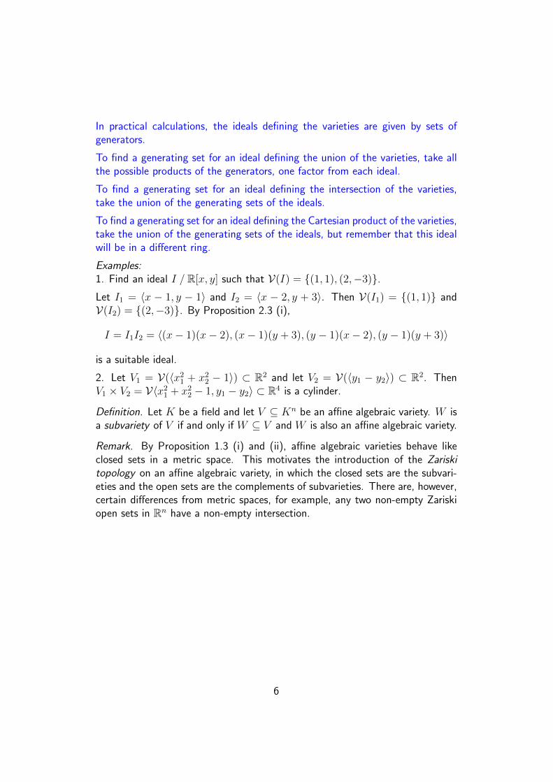
2. Let V1 = V(〈x21 + x22 − 1〉) ⊂ R2 and let V2 = V(〈y1 − y2〉) ⊂ R2. ThenV1 × V2 = V〈x21 + x22 − 1, y1 − y2〉 ⊂ R4 is a cylinder.

Definition. Let K be a field and let V ⊆ Kn be an affine algebraic variety. W isa subvariety of V if and only if W ⊆ V and W is also an affine algebraic variety.

Remark. By Proposition 1.3 (i) and (ii), affine algebraic varieties behave likeclosed sets in a metric space. This motivates the introduction of the Zariskitopology on an affine algebraic variety, in which the closed sets are the subvari-eties and the open sets are the complements of subvarieties. There are, however,certain differences from metric spaces, for example, any two non-empty Zariskiopen sets in Rn have a non-empty intersection.

6

1.2 Affine spaces

Affine spaces are the simplest algebraic varieties, they are the solutions sets ofsystem of linear equations, i. e., they are defined by ideals generated by degree1 polynomials.

Definition. Let K be a field, and let V be a finite dimension vector space overK. U ⊆ V is an affine subspace of V if and only if U = ∅ or U = u0 + W ={u0 + w | w ∈ W}, where u0 ∈ U and W is a linear subspace of V . (Linearsubspace or vector subspace of a vector space means subspace as defined inMATH10202 or MATH10212.)

Examples: Kn as a subspace of itself, ∅, any set containing a single point are allaffine subspaces of Kn. The line y = 2x+ 5 is an affine subspace of R2, in thiscase we can take W = span{(1, 2)} and u0 = (0, 5).

Proposition 1.4 Let U = u0 + W be a non-empty affine subspace in a vectorspace V . Then U = u+W for any u ∈ U , in other words, u0 can be chosen tobe an arbitrary element of U , but W is uniquely determined by U .

Proof. Let u ∈ U , then u = u0 + (u− u0), so u− u0 ∈ W . We have

u+W = {u+ w | w ∈ W} = {u0 + (u− u0) + w | w ∈ W}.

(u− u0) + w ∈ W as W is a vector space, therefore u+ w ∈ u0 +W for everyw ∈ W , hence u+W ⊆ u0 +W . Similarly,

u0 +W = {u0 + w | w ∈ W} = {u+ (u0 − u) + w | w ∈ W} ⊆ u+W,

therefore u+W = u0 +W = U .

W can be obtained as U − u = {v − u | v ∈ U} for any u ∈ U .

Definition. The dimension of an affine space U = u0 + W is defined to bedimW . (Sometimes it is convenient to define dim ∅ = −1.)

Definition. Let K be a field. Kn, considered as an affine subspace of itself iscalled an n-dimensional affine space over K, and is denoted by An(K) or An ifthe field is understood.

Definition. Let V1, V2 be vector spaces. An affine map from V1 to V2 is definedto be a function Φ : V1 → V2 which can be written in the form Φ(x) = T (x)+b,where T : V1 → V2 is a linear transformation and b ∈ V2.

It is easily checked that the composition of affine maps is also an affine map. Theinvertible affine maps V → V form a group. Within this group the translationsform a normal subgroup and the quotient by this normal subgroup is the groupof invertible linear transformations on V .

7

Proposition 1.5 (Not examinable) Let V1, V2 be vector spaces and let Φ : V1 →V2 be an affine map.(i) For any affine subspace U1 ⊆ V1, the image Φ(U1) is also an affine subspaceof V2.(ii) For any affine subspace U2 ⊆ V2, the preimage Φ−1(U2) is also an affinesubspace of V1.

Proof. Let x1, x2, . . . , xm be the co-ordinates on V1, y1, y2, . . . , yn theco-ordinates on V2. Let Φ(x) = T (x) + b, where T : V1 → V2 is a lineartransformation and b = (b1, b2, . . . , bn)T ∈ V2 is a vector. Let {tij}1≤i≤n,1≤j≤mbe the matrix of T with respect to the co-ordinates on V1 and V2.

(i) Let U1 ⊆ V1 be an affine subspace. If U1 = ∅, Φ(U1) = ∅, too. Otherwise,we can write U1 = u1 + W1, where u1 ∈ U1 and W1 is a linear subspace of V1.Then

Φ(U1) = {Φ(u1 + w) | w ∈ W1} = {T (u1 + w) + b | w ∈ W1}= {(T (u1) + b) + T (w) | w ∈ W} = (T (u1) + b) + T (W )

As T (W ) is a linear subspace of W2, it follows that Φ(U1) is an affine subspace,as claimed.

(ii) Let now U2 be an affine subspace of V2.

There exist degree 1 polynomials f1, f2, . . . , fk in y1, y2, . . . , yn such thatU2 = {(y1, y2, . . . , yn) ∈ V2 | fi(y1, y2, . . . , yn) = 0,∀i, 1 ≤ i ≤ k}.Then

Φ((x1, x2, . . . , xm)T ) =

(b1 +

m∑j=1

t1jxj, b2 +m∑j=1

t2jxj, . . . , bn +m∑j=1

tnjxj

)T,

therefore Φ((x1, x2, . . . , xm)T ) ∈ U2 if and only if

fi

(b1 +

m∑j=1

t1jxj, b2 +m∑j=1

t2jxj, . . . , bn +m∑j=1

tnjxj

)= 0

for every i, 1 ≤ i ≤ k. These are linear equations in the xi, 1 ≤ i ≤ m, thereforeΦ−1(U2) is an affine subspace of V1, as claimed.

Definition. Let X, Y be subsets of a vector space V . X and Y are affineequivalent if and only if there exist mutually inverse affine maps Φ,Ψ : V → Vsuch that Φ(X) = Y and Ψ(Y ) = X. It is easy to verify that affine equivalenceis an equivalence relation.

8

Examples:1. All affine subspaces of the same dimension are affine equivalent. This can beproved by showing that any k-dimensional affine subspace is affine equivalent tothe linear subspace spanned by the first k standard unit vectors.

2. Any two triangles in R2 are affine equivalent. An easy way to prove it is to showthat any triangle is affine equivalent to the triangle with vertices (0, 0), (1, 0)and (0, 1). See https://personalpages.manchester.ac.uk/staff/gabor.megyesi/teaching/MATH32062/triangles.pdf for an example of calculatingan explicit affine equivalence between two triangles.

3. Similarly, any two parallelograms in R2 are because all parallelograms affineequivalent to the unit square.

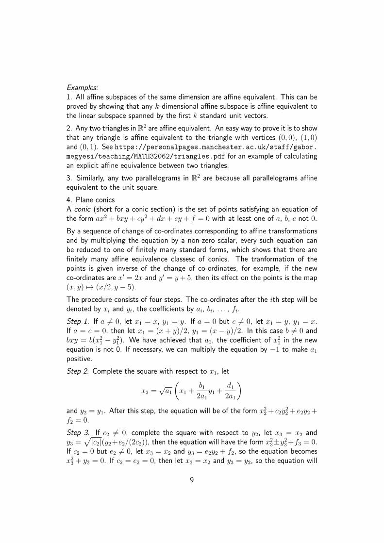
4. Plane conicsA conic (short for a conic section) is the set of points satisfying an equation ofthe form ax2 + bxy + cy2 + dx+ ey + f = 0 with at least one of a, b, c not 0.

By a sequence of change of co-ordinates corresponding to affine transformationsand by multiplying the equation by a non-zero scalar, every such equation canbe reduced to one of finitely many standard forms, which shows that there arefinitely many affine equivalence classesc of conics. The tranformation of thepoints is given inverse of the change of co-ordinates, for example, if the newco-ordinates are x′ = 2x and y′ = y+ 5, then its effect on the points is the map(x, y) 7→ (x/2, y − 5).

The procedure consists of four steps. The co-ordinates after the ith step will bedenoted by xi and yi, the coefficients by ai, bi, . . . , fi.

Step 1. If a 6= 0, let x1 = x, y1 = y. If a = 0 but c 6= 0, let x1 = y, y1 = x.If a = c = 0, then let x1 = (x + y)/2, y1 = (x − y)/2. In this case b 6= 0 andbxy = b(x21 − y21). We have achieved that a1, the coefficient of x21 in the newequation is not 0. If necessary, we can multiply the equation by −1 to make a1positive.

Step 2. Complete the square with respect to x1, let

x2 =√a1

(x1 +

b12a1

y1 +d12a1

)and y2 = y1. After this step, the equation will be of the form x22 + c2y

22 + e2y2 +

f2 = 0.

Step 3. If c2 6= 0, complete the square with respect to y2, let x3 = x2 andy3 =

√|c2|(y2+e2/(2c2)), then the equation will have the form x23±y23 +f3 = 0.

If c2 = 0 but e2 6= 0, let x3 = x2 and y3 = e2y2 + f2, so the equation becomesx23 + y3 = 0. If c2 = e2 = 0, then let x3 = x2 and y3 = y2, so the equation will

9

have the form x23 + f3 = 0.

Step 4. If f3 6= 0, then let x4 = x3/√|f3|, y4 = y3/

√|f3| and after the change

of variable divide the whole equation by |f3|. After this, the form of the equationwill be the same, but f3 will be ±1. If f3 = 0, then let x4 = x3, y4 = y3.

At the end of this step, either the equation is x24 + y4 = 0, or it contains x24,possibly ±y24 and possibly ±1 and no other term. x24 − y24 − 1 = 0 can betranformed into x24 − y24 + 1 = 0 by swapping x4 and y4, so these two are affineequivalent.

Therefore any variety in R2 defined by a degree 2 equation is affine equivalentto one of the following:

Case 1. x2 + y2 − 1 = 0 (ellipses)Case 2. x2 + y2 = 0 (single point)Case 3. x2 + y2 + 1 = 0 (∅)Case 4. x2 − y2 − 1 = 0 (hyperbolas)Case 5. x2 − y2 = 0 (two intersecting lines)Case 6. x2 + y = 0 (parabolas)Case 7. x2 − 1 = 0 (two parallel lines)Case 8. x2 = 0 (“double line”)Case 9. x2 + 1 = 0 (∅)It is also true, but requires a separate proof, that these cases, apart fromthe two empty sets are not affine equivalent. See https://personalpages.

manchester.ac.uk/staff/gabor.megyesi/teaching/MATH32062/conic.pdf

for examples of transforming the equation of a conic to one of the above forms.

Over C we can use essentially the same method to reduce the equation of a conicto one of the above forms. The difference is that we do not need to multiply theequation to ensure a1 > 0 in Step 1 and there is no need to take the modulusof c2 and f3 in Steps 2 and 3, resp. If a term occurs in the final equation, it willalways have coefficient +1, so we will end up with one of Cases 3, 6, 8 or 9.

Over C, the change of co-ordinates x′ = x, y′ = iy converts Case 1 into Case 4and vice versa, so all ellipses and hyperbolas are affine equivalent over C. By asimilar argument, Cases 1, 3 and 4 are affine equivalent over C, similarly Cases2 and 5, and Cases 7 and 9.

10

1.3 The correspondence between varieties and ideals

Definition. Let X ⊆ An. The ideal of X is defined as

I(X)={f ∈ K[x1, x2, . . . , xn] | f(a1, a2, . . . , an) = 0,∀(a1, a2, . . . , an) ∈ X}.

I(X) is an indeed ideal of K[x1, x2, . . . , xn].

It is clear from the definition that X1 ⊆ X2 implies I(X1) ⊇ I(X2).

Proposition 1.6(i) If J / K[x1, x2, . . . , xn], then J ⊆ I(V(J)).(ii) X ⊆ V(I(X)) for any X ⊆ An(K). Equality holds if and only if X is anaffine algebraic variety.

Proof. (i) If f ∈ J and P ∈ V(J) then f(P ) = 0 by the definition of V , thereforef ∈ I(V(J)) by the definition of I, so J ⊆ I(V(J)) as claimed.

(ii) It is also clear from the definitions that X ⊆ V(I(X)) for any set X ⊆ An

and that if equality holds then X is an affine algebraic variety.

The only thing that remains to be proved that if X is an algebraic variety, thenX = V(I(X)). Assume that X = V(J) for some ideal J / K[x1, x2, . . . , xn].By (i), J ⊆ I(V(J)), therefore X = V(J) ⊇ V(I(V(J))) = V(I(X)). We havealready seen that X ⊆ V(I(X)), therefore X = V(I(X)), as required.

Definition. A field K is algebraically closed if and only if every polynomial ofdegree at least 1 in K[x] has a root in K.

Examples: C and Q̄ (the field of algebraic numbers in C) are algebraically closed.Q, R and the finite fields are not algebraically closed.

Remark. For any field K, there exists a minimal algebraically closed field con-taining it, which is unique up to isomorphism, this field is called the algebraicclosure of K. For example, the algebraic closure of R is C and the algebraicclosure of Q is Q̄Definition. Let R be a (commutative) ring. Let I / R be an ideal. The radicalof I, denoted by

√I or rad I, is

√I = {a ∈ R | ∃n ∈ N such that an ∈ I}.

I is called a radical ideal if and only if√I = I.

Algebraic facts: For any ideal I,√I is also an ideal, I ⊆

√I and

√√I =√I,

i. e.,√I is a radical ideal.

11

Theorem 1.7 (Hilbert’s Nullstellensatz) Let K be an algebraically closed field.(i) Every maximal ideal of K[x1, x2, . . . , xn] is of the form 〈x1−a1, x2−a2, . . . , xn−an〉, where ai ∈ K, 1 ≤ i ≤ n.(ii) If J is an ideal of K[x1, x2, . . . , xn], J 6= K[x1, x2, . . . , xn] , then V(J) 6= ∅.(iii) I(V(J)) =

√J for any J / K[x1, x2, . . . , xn].

Proof. (i) Not proved here.

Note that 〈x1−a1, x2−a2, . . . , xn−an〉 is a maximal ideal of K[x1, x2, . . . , xn]for any field K. We can define a ring homomorphism K[x1, x2, . . . , xn] → K,f 7→ f(a1, a2, . . . , an), whose kernel is exactly 〈x1 − a1, x2 − a2, . . . , xn − an〉.Since the image is a field, the kernel is a maximal ideal. The substance of thispart is that over an algebraically closed field the converse is also true.

(ii) As J 6= K[x1, x2, . . . , xn], there exists a maximal ideal m containing J .By (i), m = 〈x1 − a1, x2 − a2, . . . , xn − an〉 for some ai ∈ K, 1 ≤ i ≤ n.Therefore {(a1, a2, . . . , an)} = V(m) ⊆ V(J), so V(J) 6= ∅.(iii) If f ∈

√J , then fk ∈ J for some positive integer k. Hence fk(P ) =

(f(P ))k = 0 for every P ∈ V(J), therefore f(P ) = 0 for every P ∈ V(J), i. e.,f ∈ I(V(J)). This means that

√J ⊆ I(V(J)) without assuming that K is

algebraically closed.

We need to prove the other inclusion, I(V(J)) ⊆√J . Let f ∈ I(V(J)). Let’s

introduce a new variable y. Let f1, f2, . . . , fr be a set of generators for J , andlet J1 = 〈f1, f2, . . . , fr, fy − 1〉 / K[x1, x2, . . . , xn, y].

We claim that V(J1) = ∅. Assume that P = (a1, a2, . . . , an, b) ∈ V(J1) ⊆ An+1.As fi ∈ J1 for every i, 1 ≤ i ≤ r, we have fi(a1, a2, . . . , an) = 0 for every i,1 ≤ i ≤ r, so (a1, a2, . . . , an) ∈ V(J). Therefore f(a1, a2, . . . , an) = 0, too,but then (fy − 1)(P ) = −1, so P /∈ V(J1) after all. Therefore V(J1) = ∅, asclaimed.

By (ii), this implies that J1 = K[x1, x2, . . . , xn, y], in particular 1 ∈ J1. Thismeans that we can write

1 = (fy − 1)g0 +r∑i=1

gifi

for suitable g0, g1, . . . , gr ∈ K[x1, x2, . . . , xn, y]. Let yN be the highest powerof y occurring in any of g0, g1, . . . , gr. Let’s multiply the above equality by fN .Whenever there is a power y, say yk, occurring in gi for some i, 0 ≤ i ≤ r, we canwrite ykfN as (fy)kfN−k, so for each i, 0 ≤ i ≤ r, fNgi(x1, x2, . . . , xn, y) =

12

Gi(x1, x2, . . . , xn, fy) for a suitable polynomial Gi. Therefore

fN = (fy − 1)G0(x1, x2, . . . , xn, fy) +r∑i=1

fiGi(x1, x2, . . . , xn, fy).

By substituting y = 1/f into the above equality, we obtain

fN =r∑i=1

fiGi(x1, x2, . . . , xn, 1).

The right-hand side is an element of J , therefore f ∈√J as required.

The function V from ideals of K[x1, x2, . . . , xn] to affine algebraic varietiesin An is not injective, and the function I from subsets of An to ideals ofK[x1, x2, . . . , xn] is neither injective nor surjective. However, the combination ofProposition 1.6 and the Nullstellensatz implies that V and I create a bijectionbetween radical ideals of K[x1, x2, . . . , xn] and affine algebraic varieties in An.

13

1.4 Irreducibility

Definition. An affine algebraic variety W is reducible if and only if it can bewritten as W = V1 ∪ V2, where W1, W2 are also affine algebraic varieties,W1 6= V 6= V2. If W is not reducible, it is called irreducible. (The irreducibilityof W is equivalent to saying that if W = V1 ∪ V2, where W1, W2 are also affinealgebraic varieties, then W1 = V or W2 = V .)

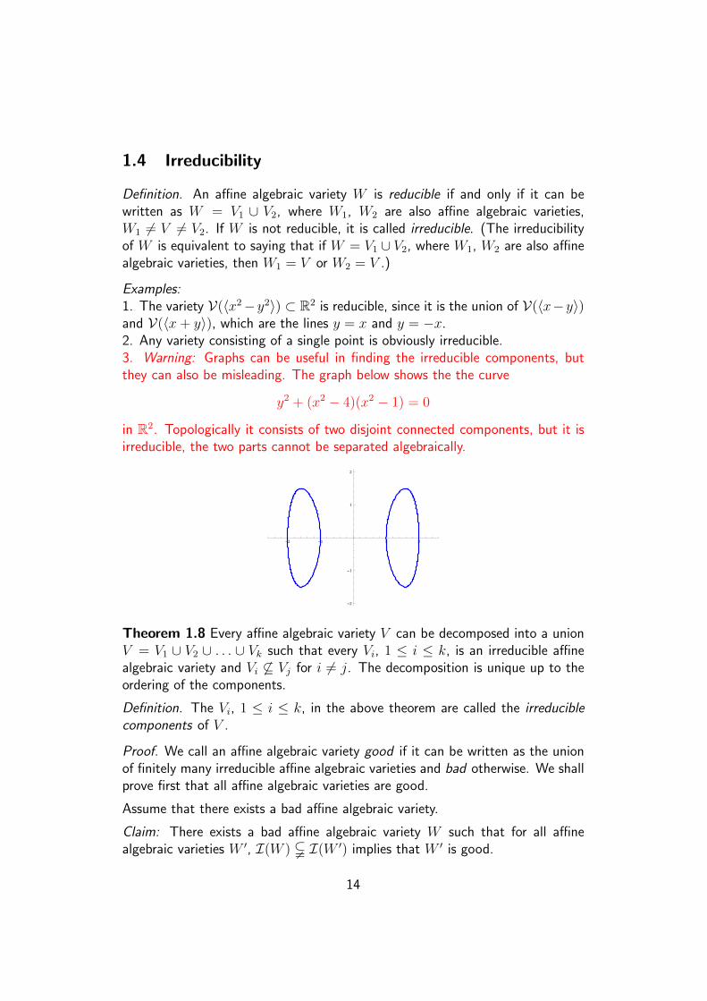
Examples:1. The variety V(〈x2−y2〉) ⊂ R2 is reducible, since it is the union of V(〈x−y〉)and V(〈x+ y〉), which are the lines y = x and y = −x.2. Any variety consisting of a single point is obviously irreducible.3. Warning: Graphs can be useful in finding the irreducible components, butthey can also be misleading. The graph below shows the the curve

y2 + (x2 − 4)(x2 − 1) = 0

in R2. Topologically it consists of two disjoint connected components, but it isirreducible, the two parts cannot be separated algebraically.

-2 -1 1 2

-2

-1

1

2

Theorem 1.8 Every affine algebraic variety V can be decomposed into a unionV = V1 ∪ V2 ∪ . . . ∪ Vk such that every Vi, 1 ≤ i ≤ k, is an irreducible affinealgebraic variety and Vi 6⊆ Vj for i 6= j. The decomposition is unique up to theordering of the components.

Definition. The Vi, 1 ≤ i ≤ k, in the above theorem are called the irreduciblecomponents of V .

Proof. We call an affine algebraic variety good if it can be written as the unionof finitely many irreducible affine algebraic varieties and bad otherwise. We shallprove first that all affine algebraic varieties are good.

Assume that there exists a bad affine algebraic variety.

Claim: There exists a bad affine algebraic variety W such that for all affinealgebraic varieties W ′, I(W ) $ I(W ′) implies that W ′ is good.

14

Assume that this claim is false. Let V1 be a bad affine algebraic variety, thenthere exists a bad variety V2 such that I(V1) $ I(V2). Similarly, there exists abad variety V3 such that I(V2) $ I(V3). Continuing like this, we can constructan infinite sequence of bad varieties V1, V2, V3, . . . , such that

I(V1) $ I(V2) $ I(V3) $ . . . $ I(Vm) $ I(Vm+1) $ . . . .

The I(Vm), m = 1, 2, 3, . . . are ideals in the polynomial ring K[x1, x2, . . . , xn]for some n, which is Noetherian by the Hilbert Basis Theorem (Theorem 1.2),so it does not contain a strictly increasing infinite sequence of ideals. Thiscontradiction shows that the claim is true.

Let now W be a bad affine algebraic variety with the property described in theclaim. W cannot be irreducible, since any irreducible variety is good, becauseit is the union of one irreducible variety. Therefore W is reducible, there existaffine algebraic varieties W1 and W2 such that W1 6= W 6= W2 and W =W1 ∪ W2. Wi ⊂ W implies I(Wi) ⊇ I(W ) for i = 1, 2. By Proposition1.6 (ii), V(I(W )) = W and V(I(Wi)) = Wi for i = 1, 2, so Wi 6= W impliesI(Wi) % I(W ) for i = 1, 2. By the assumption on W , this implies that W1 andW2 are both good, they are unions of finitely many irreducible affine algebraicvarieties. Then W = W1∪W2 is also the union of finitely many irreducible affinealgebraic varieties, contradicting the assumption that W is bad.

This shows that every affine algebraic variety V can be written as a finite unionof irreducible affine algebraic varieties, then discarding the varieties which arecontained in one of the terms, we can write V = V1 ∪ V2 . . . ∪ Vk with Viirreducible for each i, 1 ≤ i ≤ k and Vi 6⊆ Vj if i 6= j.

Let V = V ′1 ∪ V ′2 ∪ . . . ∪ V ′l be another decomposition of V into irreduciblevarieties with V ′i 6⊆ V ′j for i 6= j. Then

V1 = V1 ∩ V = (V1 ∩ V ′1) ∪ (V1 ∩ V ′2) ∪ . . . ∪ (V1 ∩ V ′l ).

As V1 is irreducible, there exists i such that V1 = V1 ∩ V ′i , i. e., V1 ⊆ V ′i . Byapplying this argument to V ′i , we obtain that there exists j such that V ′i ⊆ Vj,therefore V1 ⊆ Vj. This implies j = 1 by our assumption on the V1, V2, . . . , Vk,and therefore V1 = V ′i .

By applying this argument to each Vr (1 ≤ r ≤ k) and V ′s (1 ≤ s ≤ l), we obtaina bijection between {V1, V2, . . . , Vk} and {V ′1 , V ′2 , . . . , V ′l }, so the decompositionsare the same apart from possibly the order of the components.

Definition. Let R be a commutative ring. An ideal I / R is called a prime idealif and only if ab ∈ I implies a ∈ I or b ∈ I.

Proposition 1.9 An affine algebraic variety W is irreducible if and only if I(W )is prime.

15

Proof. We shall prove the contrapositive, namely that W is reducible if and onlyif I(W ) is not prime.

Assume that W is reducible, then W can be written as W = W1∪W2, where W1

and W2 are affine algebraic varieties and W 6= W1, W 6= W2. W1 ⊂ W impliesI(W1) ⊇ I(W ), but V(I(W )) = W and V(I(W1)) = W1 by Proposition1.6 (ii), therefore I(W1) 6= I(W ), so I(W1) % I(W ). Let f1 ∈ I(W1) \I(W ).Similarly, let f2 ∈ I(W2) \ I(W ). If P ∈ W1, then (f1f2)(P ) = 0 becausef1(P ) = 0, if P ∈ W2, then (f1f2)(P ) = 0 because f2(P ) = 0, therefore(f1f2)(P ) = 0 for every P ∈ W , so f1f2 ∈ I(W ). Neither f1, nor f2 is anelement of I(W ), therefore I(W ) is not prime. This shows that if I(W ) isprime, then W is irreducible.

Assume now that I(W ) is not prime. Let f1, f2 be polynomials such that f1,f2 /∈ I(W ), but f1f2 ∈ I(W ). Let

W1 = {P ∈ W | f1(P ) = 0} = W ∩ V(〈f1〉) = V(〈I(W ), f1〉)

and similarly

W2 = {P ∈ W | f2(P ) = 0} = W ∩ V(〈f2〉) = V(〈I(W ), f2〉).

W1, W2 are affine algebraic varieties. Clearly W1 ⊆ W , W2 ⊆ W , but W1 6= Wsince f1 /∈ I(W ) and similarly W2 6= W since f2 /∈ I(W ). For any P ∈ W ,0 = (f1f2)(P ) = f1(P )(f2)(P ), so f1(P ) = 0 or f2(P ) = 0. In the first case,P ∈ W1, in the second P ∈ W2, therefore W = W1 ∪W2 and W is reducible.This shows that if W is irreducible, then I(W ) is prime.

Remark. The criterion involves I(W ), so if W = V(J) for some ideal J , theprimality or otherwise of J is not sufficient in general to tell whether W isirreducible or not. If the field is algebraically closed, then I(V(J)) =

√J by the

Nullstellensatz. If J is prime, then it is automatically radical, so I(V(J)) = Jand V(J) is irreducible. If J is radical but not prime, then V(J) is reducible.

The functions V and I create a bijection between prime ideals of K[x1, x2, . . . , xn]and irreducible affine algebraic varieties in An.

Properties of irreducible varieties and examples

1. Irreducibility is preserved under affine equivalence. If X and Y are affineequivalent affine algebraic varieties, then X is irreducible if and only if Y is.Let Φ : X → Y be an affine equivalence and assume that X can be written asX = X1∪X2, where X1, X2 are also affine algebraic varieties and X1 6= X 6= X2,then Y = Φ(X1) ∪ Φ(X2), Φ(X1), Φ(X2) are also affine algebraic varieties andΦ(X1) 6= Y 6= Φ(X2).

16

2. Affine subspaces over an infinite field K are irreducible. (Note that alge-braically closed fields are infinite.) Every affine subspace is equivalent to oneof the form x1 = x2 = . . . = xk = 0 for some k. It can be proved thatI(V(〈x1, x2, . . . , xk〉)) = 〈x1, x2, . . . , xk〉 if K is infinite and that 〈x1, x2, . . . , xk〉/K[x1, x2, . . . , xn] is a prime ideal directly from the definition.

3. Let K be an algebraically closed field. Let H ⊂ An(K) be a hypersurface,that is, an algebraic variety defined by an ideal generated by a single polynomialf ∈ K[x1, x2, . . . , xn], H = V(〈f〉). f can be factorised as f = fα1

1 fα22 · · · fαr

r ,where the fi, 1 ≤ i ≤ r, are irreducible polynomials such that fi is not a scalarmultiple of fj if i 6= j, and αi, 1 ≤ i ≤ r, are positive integers. This factorisationis unique up to scalar factors.

We shall now show that√〈f〉 = 〈f1f2 · · · fr〉. Let g ∈

√〈f〉. g can be

factorised as g = gβ11 gβ22 · · · gβss , where the gi, 1 ≤ i ≤ s, are irreducible poly-

nomial such that gi is not a scalar multiple of gj if i 6= j, and βi, 1 ≤ i ≤ s,

are positive integers. g ∈√〈f〉 means that there exists a positive integer

m such that gm = gmβ11 gmβ22 · · · gmβss ∈ 〈f〉, therefore for each i, 1 ≤ i ≤ r,fi|gmβ11 gmβ22 · · · gmβss . As fi is irreducible, it must divide gj for some j, 1 ≤ j ≤ s,so fi|g. The fi are pairwise coprime, therefore it follows that f1f2 . . . fr|g,g ∈ 〈f1f2 · · · fr〉. Conversely, if g ∈ 〈f1f2 · · · fr〉, then gmax{α1,α2,...,αr} ∈ 〈f〉.This shows that I(H) =

√〈f〉 = 〈f1f2 · · · fr〉.

By Proposition 1.3 (i),⋃ri=1 V(〈fi〉) = V〈f1f2 · · · fr〉 = H. By the argument

used previously, 〈fi〉 / K[x1, x2, . . . , xn] is a prime ideal, therefore it is radical,so I(V(〈fi〉)) = 〈fi〉 by the Nullstellensatz, by using the fact that 〈fi〉 is primeagain, it follows that V(〈fi〉) is irreducible. V(〈fi〉) does not contain V(〈fj〉)if i 6= j, because fj is not a multiple of fi. This shows that the irreduciblecomponents are V(〈fi〉), 1 ≤ i ≤ r.

In particular, H is irreducible if and only if r = 1, i. e., f is the power of a singleirreducible polynomial.

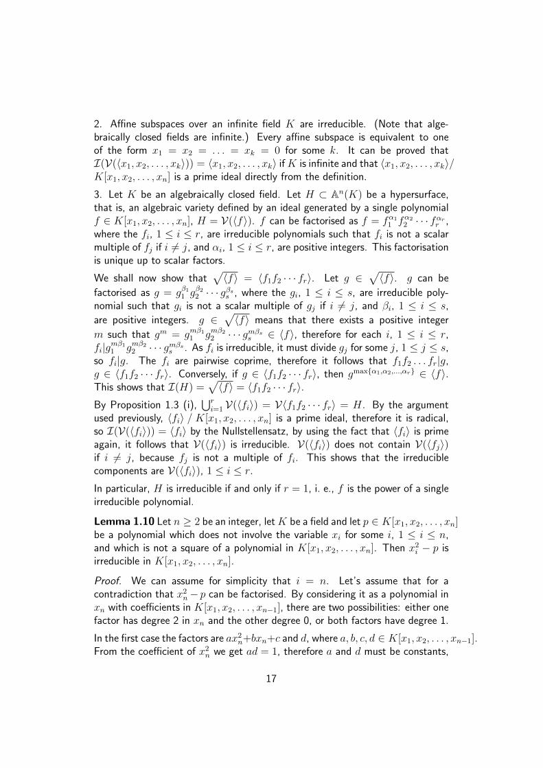
Lemma 1.10 Let n ≥ 2 be an integer, let K be a field and let p ∈ K[x1, x2, . . . , xn]be a polynomial which does not involve the variable xi for some i, 1 ≤ i ≤ n,and which is not a square of a polynomial in K[x1, x2, . . . , xn]. Then x2i − p isirreducible in K[x1, x2, . . . , xn].

Proof. We can assume for simplicity that i = n. Let’s assume that for acontradiction that x2n− p can be factorised. By considering it as a polynomial inxn with coefficients in K[x1, x2, . . . , xn−1], there are two possibilities: either onefactor has degree 2 in xn and the other degree 0, or both factors have degree 1.

In the first case the factors are ax2n+bxn+c and d, where a, b, c, d ∈ K[x1, x2, . . . , xn−1].From the coefficient of x2n we get ad = 1, therefore a and d must be constants,

17

so we do not get a proper factorisation.

In the second case the factors are axn+b and cxn+d with a, b, c, d ∈ K[x1, x2, . . . , xn−1].Similarly to the previous case, from the coefficient of x2n we get ac = 1, thereforea and c must be constants. By dividing the first factor by a and multiplying thesecond by a, we can assume that a = c = 1. Then x2n− p = (xn + b)(xn + d) =x2n+ (b+d)xn+ bd, so by comparing the coefficient of xn and the degree 0 termin xn we get b + d = 0 and −p = bd. Hence d = −b, so −p = −b2, p = b2,but p is not a square, this is a contradiction, therefore x2n − p is irreducible asclaimed. .

This simple lemma has lots of useful consequences.

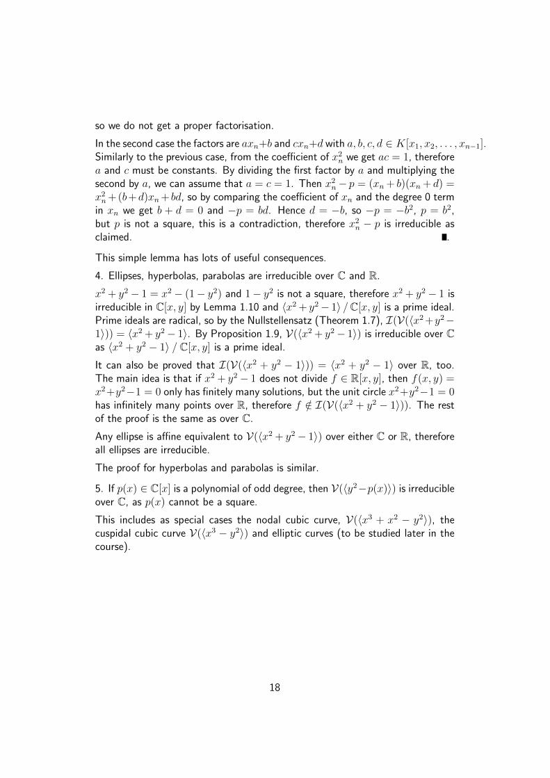
4. Ellipses, hyperbolas, parabolas are irreducible over C and R.

x2 + y2 − 1 = x2 − (1− y2) and 1− y2 is not a square, therefore x2 + y2 − 1 isirreducible in C[x, y] by Lemma 1.10 and 〈x2 + y2− 1〉 /C[x, y] is a prime ideal.Prime ideals are radical, so by the Nullstellensatz (Theorem 1.7), I(V(〈x2+y2−1〉)) = 〈x2 + y2− 1〉. By Proposition 1.9, V(〈x2 + y2− 1〉) is irreducible over Cas 〈x2 + y2 − 1〉 / C[x, y] is a prime ideal.

It can also be proved that I(V(〈x2 + y2 − 1〉)) = 〈x2 + y2 − 1〉 over R, too.The main idea is that if x2 + y2− 1 does not divide f ∈ R[x, y], then f(x, y) =x2+y2−1 = 0 only has finitely many solutions, but the unit circle x2+y2−1 = 0has infinitely many points over R, therefore f /∈ I(V(〈x2 + y2 − 1〉)). The restof the proof is the same as over C.

Any ellipse is affine equivalent to V(〈x2 + y2− 1〉) over either C or R, thereforeall ellipses are irreducible.

The proof for hyperbolas and parabolas is similar.

5. If p(x) ∈ C[x] is a polynomial of odd degree, then V(〈y2−p(x)〉) is irreducibleover C, as p(x) cannot be a square.

This includes as special cases the nodal cubic curve, V(〈x3 + x2 − y2〉), thecuspidal cubic curve V(〈x3 − y2〉) and elliptic curves (to be studied later in thecourse).

18

-1 1 2

-4

-2

2

4

-0.5 0.5 1.0 1.5 2.0 2.5

-4

-2

2

4

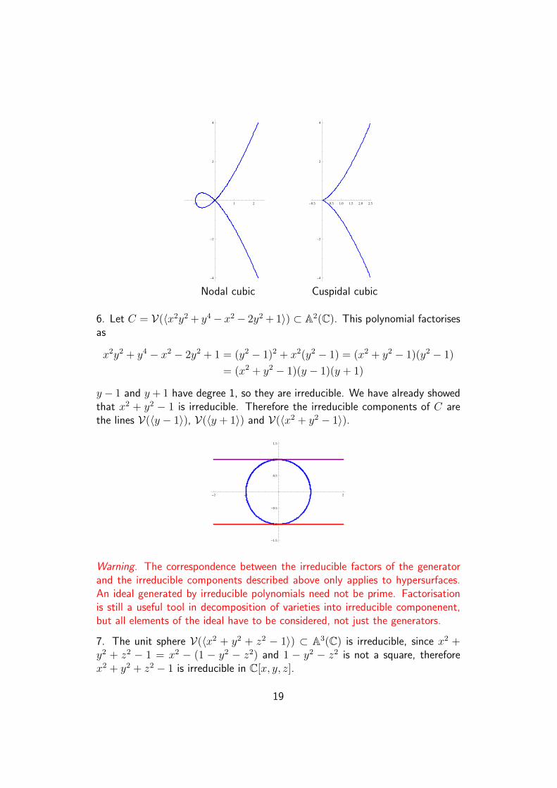
Nodal cubic Cuspidal cubic

6. Let C = V(〈x2y2 + y4− x2− 2y2 + 1〉) ⊂ A2(C). This polynomial factorisesas

x2y2 + y4 − x2 − 2y2 + 1 = (y2 − 1)2 + x2(y2 − 1) = (x2 + y2 − 1)(y2 − 1)

= (x2 + y2 − 1)(y − 1)(y + 1)

y − 1 and y + 1 have degree 1, so they are irreducible. We have already showedthat x2 + y2 − 1 is irreducible. Therefore the irreducible components of C arethe lines V(〈y − 1〉), V(〈y + 1〉) and V(〈x2 + y2 − 1〉).

-2 -1 1 2

-1.5

-1.0

-0.5

0.5

1.0

1.5

Warning. The correspondence between the irreducible factors of the generatorand the irreducible components described above only applies to hypersurfaces.An ideal generated by irreducible polynomials need not be prime. Factorisationis still a useful tool in decomposition of varieties into irreducible componenent,but all elements of the ideal have to be considered, not just the generators.

7. The unit sphere V(〈x2 + y2 + z2 − 1〉) ⊂ A3(C) is irreducible, since x2 +y2 + z2 − 1 = x2 − (1 − y2 − z2) and 1 − y2 − z2 is not a square, thereforex2 + y2 + z2 − 1 is irreducible in C[x, y, z].

19

It can be proved that I(V(〈x2 + y2 + z2 − 1〉)) = 〈x2 + y2 + z2 − 1〉 over Rsimilarly to the case of the circle, therefore the unit sphere is also irreducible overR.

Any ellipsoid is affine equivalent to the unit sphere, therefore ellipsoids are irre-ducible over R or C.

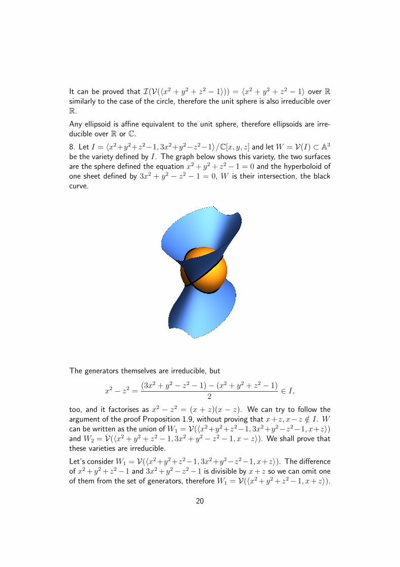
8. Let I = 〈x2+y2+z2−1, 3x2+y2−z2−1〉/C[x, y, z] and let W = V(I) ⊂ A3

be the variety defined by I. The graph below shows this variety, the two surfacesare the sphere defined the equation x2 + y2 + z2− 1 = 0 and the hyperboloid ofone sheet defined by 3x2 + y2 − z2 − 1 = 0, W is their intersection, the blackcurve.

The generators themselves are irreducible, but

x2 − z2 =(3x2 + y2 − z2 − 1)− (x2 + y2 + z2 − 1)

2∈ I,

too, and it factorises as x2 − z2 = (x + z)(x − z). We can try to follow theargument of the proof Proposition 1.9, without proving that x+z, x−z /∈ I. Wcan be written as the union of W1 = V(〈x2+y2+z2−1, 3x2+y2−z2−1, x+z〉)and W2 = V(〈x2 + y2 + z2 − 1, 3x2 + y2 − z2 − 1, x− z〉). We shall prove thatthese varieties are irreducible.

Let’s consider W1 = V(〈x2+y2+z2−1, 3x2+y2−z2−1, x+z〉). The differenceof x2 + y2 + z2−1 and 3x2 + y2− z2−1 is divisible by x+ z so we can omit oneof them from the set of generators, therefore W1 = V(〈x2 + y2 + z2− 1, x+ z〉).

20

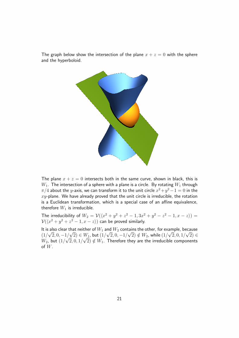
The graph below show the intersection of the plane x + z = 0 with the sphereand the hyperboloid.

The plane x + z = 0 intersects both in the same curve, shown in black, this isW1. The intersection of a sphere with a plane is a circle. By rotating W1 throughπ/4 about the y-axis, we can transform it to the unit circle x2+y2−1 = 0 in thexy-plane. We have already proved that the unit circle is irreducible, the rotationis a Euclidean transformation, which is a special case of an affine equivalence,therefore W1 is irreducible.

The irreducibility of W2 = V(〈x2 + y2 + z2 − 1, 3x2 + y2 − z2 − 1, x − z〉) =V(〈x2 + y2 + z2 − 1, x− z〉) can be proved similarly.

It is also clear that neither of W1 and W2 contains the other, for example, because(1/√

2, 0,−1/√

2) ∈ W1, but (1/√

2, 0,−1/√

2) /∈ W2, while (1/√

2, 0, 1/√

2) ∈W2, but (1/

√2, 0, 1/

√2) /∈ W1. Therefore they are the irreducible components

of W .

21