MATH685Z – Mathematical Models in Financial Economics

Topic 6 — Mean variance portfolio theory

6.1 Markowitz mean-variance formulation

6.2 Two-fund Theorem

6.3 Inclusion of the risk free asset: One-fund Theorem

6.4 Addition of risk tolerance factor

6.5 Asset - liability model

1

6.1 Markowitz mean-variance formulation

We consider a single-period investment model. Suppose there are N

risky assets, whose rates of return are given by the random variables

r1, · · · , rN , where

rn =Sn(1) − Sn(0)

Sn(0), n = 1,2, · · · , N.

Here Sn(0) is known while Sn(1) is random, n = 1,2, · · · , N . Let

w = (w1 · · ·wN)T , wn denotes the proportion of wealth invested in

asset n, withN∑

n=1

wn = 1. The rate of return of the portfolio rP is

rP =N∑

n=1

wnrn.

2

Assumptions

1. There does not exist any asset that is replicable by a combination

of other assets in the portfolio. That is, no redundant asset.

2. The two vectors µ = (r1 r2 · · · rN) and 1 = (1 1 · · ·1) are

linearly independent. If otherwise, the mean rates of return are

equal. The purpose of this assumption is to avoid the occurrence

of the degenerate case.

The first two moments of rP are

µP = E[rP ] =N∑

n=1

E[wnrn] =N∑

n=1

wnµn, where µn = rn,

and

σ2P = var(rP ) =

N∑

i=1

N∑

j=1

wiwjcov(ri, rj) =N∑

i=1

N∑

j=1

wiwjσij.

3

Covariance matrix

Let Ω denote the covariance matrix so that

σ2P = w

TΩw,

where Ω is symmetric and (Ω)ij = σij = cov(ri, rj). For example,

when n = 2, we have

(w1 w2)

(

σ11 σ12σ21 σ22

)(

w1w2

)

= w21σ2

1 + w1w2(σ12 + σ21) + w22σ2

2.

Since portfolio variance σ2P must be non-negative, so the covari-

ance matrix must be symmetric and semi-positive definite. The

eigenvalues are all real non-negative.

4

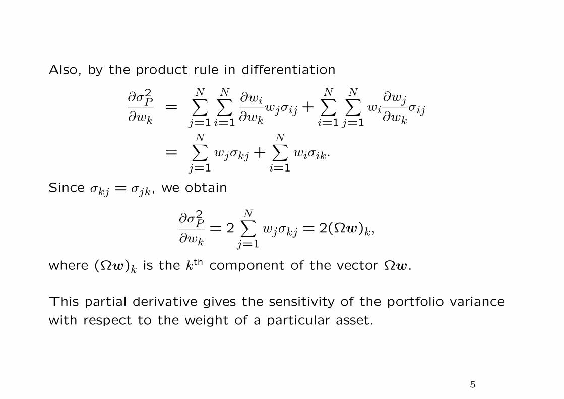
Also, by the product rule in differentiation

∂σ2P

∂wk=

N∑

j=1

N∑

i=1

∂wi

∂wkwjσij +

N∑

i=1

N∑

j=1

wi∂wj

∂wkσij

=N∑

j=1

wjσkj +N∑

i=1

wiσik.

Since σkj = σjk, we obtain

∂σ2P

∂wk= 2

N∑

j=1

wjσkj = 2(Ωw)k,

where (Ωw)k is the kth component of the vector Ωw.

This partial derivative gives the sensitivity of the portfolio variance

with respect to the weight of a particular asset.

5

Remark

1. The portfolio risk of return is quantified by σ2P . In the mean-

variance analysis, only the first two moments are considered in

the portfolio investment model. Earlier investment theory prior

to Markowitz only considered the maximization of µP without

σP .

2. The measure of risk by variance would place equal weight on the

upside and downside deviations. In reality, positive deviations

should be more welcomed.

3. The assets are characterized by their random rates of return,

ri, i = 1, · · · , N . In the mean-variance model, it is assumed that

their first and second order moments: µi, σi and σij are all known.

In our formulation, we would like to determine the choice vari-

ables: w1, · · · , wN such that σ2P is minimized for a given preset

value of µP .

6

Two-asset portfolio

Consider a portfolio of two assets with known means r1 and r2,

variances σ21 and σ2

2, of the rates of return r1 and r2, together with

the correlation coefficient ρ, where cov(r1, r2) = ρσ1σ2.

Let 1 − α and α be the weights of assets 1 and 2 in this two-asset

portfolio.

Portfolio mean: rP = (1 − α)r1 + αr2,

Portfolio variance: σ2P = (1 − α)2σ2

1 + 2ρα(1 − α)σ1σ2 + α2σ22.

7

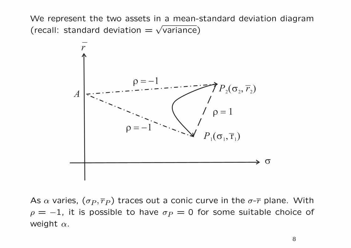
We represent the two assets in a mean-standard deviation diagram

(recall: standard deviation =√

variance)

As α varies, (σP , rP ) traces out a conic curve in the σ-r plane. With

ρ = −1, it is possible to have σP = 0 for some suitable choice of

weight α.

8

Consider the special case where ρ = 1,

σP (α; ρ = 1) =√

(1 − α)2σ21 + 2α(1 − α)σ1σ2 + α2σ2

2

= (1 − α)σ1 + ασ2.

Since rP and σP are linear in α, and if we choose 0 ≤ α ≤ 1, then

the portfolios are represented by the straight line joining P1(σ1, r1)

and P2(σ2, r2).

When ρ = −1, we have

σP (α; ρ = −1) =

√

[(1 − α)σ1 − ασ2]2 = |(1 − α)σ1 − ασ2|.

When α is small (close to zero), the corresponding point is close to

P1(σ1, r1). The line AP1 corresponds to

σP (α; ρ = −1) = (1 − α)σ1 − ασ2.

The point A corresponds to α =σ1

σ1 + σ2. It is a point on the vertical

axis which has zero value of σP .

9

The quantity (1 − α)σ1 − ασ2 remains positive until α =σ1

σ1 + σ2.

When α >σ1

σ1 + σ2, the locus traces out the upper line AP2.

Suppose −1 < ρ < 1, the minimum variance point on the curve that

represents various portfolio combinations is determined by

∂σ2P

∂α= −2(1 − α)σ2

1 + 2ασ22 + 2(1 − 2α)ρσ1σ2 = 0

↑set

giving

α =σ21 − ρσ1σ2

σ21 − 2ρσ1σ2 + σ2

2

.

10

Mean-standard deviation diagram

11

Mathematical formulation of Markowitz’s mean-variance analysis

minimize1

2

N∑

i=1

N∑

j=1

wiwjσij

subject toN∑

i=1

wiri = µP andN∑

i=1

wi = 1. Given the target expected

rate of return of portfolio µP , we find the optimal portfolio strategy

that minimizes σ2P .

Solution

We form the Lagrangian

L =1

2

N∑

i=1

N∑

j=1

wiwjσij − λ1

N∑

i=1

wi − 1

− λ2

N∑

i=1

wiri − µP

where λ1 and λ2 are the Lagrangian multipliers.

12

We then differentiate L with respect to wi and the Lagrangian mul-

tipliers, and set all the derivatives be zero.

∂L

∂wi=

N∑

j=1

σijwj − λ1 − λ2ri = 0, i = 1,2, · · · , N. (1)

∂L

∂λ1=

N∑

i=1

wi − 1 = 0; (2)

∂L

∂λ2=

N∑

i=1

wiri − µP = 0. (3)

From Eq. (1), we deduce that the optimal portfolio vector weight

w∗ admits solution of the form

w∗ = Ω−1(λ11+ λ2µ)

where 1 = (1 1 · · ·1)T and µ = (r1 r2 · · · rN)T .

13

Degenerate case

Consider the case where all assets have the same expected rate

of return, that is, µ = h1 for some constant h. In this case,

the solution to Eqs. (2) and (3) gives µP = h. The assets are

represented by points that all lie on the horizontal line: r = h.

In this case, the expected portfolio return cannot be arbitrarily pre-

scribed. Automatically, we have to take µP = h, so the constraint

on the expected portfolio return becomes irrelevant.

14

Solution procedure

To determine λ1 and λ2, we apply the two constraints:

1 = 1TΩ−1Ωw

∗ = λ11TΩ−11+ λ21

TΩ−1

µ

µP = µTΩ−1Ωw

∗ = λ1µTΩ−11+ λ2µ

TΩ−1µ.

Writing a = 1TΩ−11, b = 1T

Ω−1µ and c = µ

TΩ−1µ, we have two

equations for λ1 and λ2:

1 = λ1a + λ2b and µP = λ1b + λ2c.

Solving for λ1 and λ2:

λ1 =c − bµP

∆and λ2 =

aµP − b

∆,

where ∆ = ac − b2. Provided that µ 6= h1 for some scalar h, we

then have ∆ 6= 0.

15

Solution to the minimum portfolio variance

• λ1 and λ2 have dependence on µP , where µP is the target mean

prescribed in the variance minimization problem.

• σ2P = w

TΩw ≥ 0, for all w, so Ω is guaranteed to be semi-

positive definite. In our subsequent analysis, we assume Ω to be

positive definite. In this case, Ω−1 exists and it is also positive

definite, so a > 0, c > 0. By virtue of the Cauchy-Schwarz

inequality, ∆ > 0. Since a and ∆ are both positive, the quantity

aµ2P − 2µP + C is guaranteed to be positive.

• The minimum portfolio variance for a given value of µP is given

by

σ2P = w

∗TΩw

∗ = w∗T

Ω(λ1Ω−11+ λ2Ω

−1µ)

= λ1 + λ2µP =aµ2

P − 2bµP + c

∆.

16

The set of minimum variance portfolios is represented by a parabolic

curve in the σ2P − µP plane. The parabolic curve is generated by

varying the value of the parameter µP .

Non-optimal portfolios are represented by points which must fall on

the right side of the parabolic curve.

17

Global minimum variance portfolio

Given µP , we obtain λ1 =c − bµP

∆and λ2 =

aµP − b

∆, and the optimal

weight w∗ = Ω−1(λ11+ λ2µ).

To find the global minimum variance portfolio, we set

dσ2P

dµP=

2aµP − 2b

∆= 0

so that µP = b/a and σ2P = 1/a. Correspondingly, λ1 = 1/a and

λ2 = 0. The weight vector that gives the global minimum variance

portfolio is found to be

wg = λ1Ω−11 =

Ω−11a

=Ω−11

1TΩ−11

.

18

Two-parameter (λ1 − λ2) family of minimum variance portfolios

It is not surprising to see that λ2 = 0 corresponds to w∗g since

the constraint on the targeted mean vanishes when λ2 is taken to

be zero. In this case, we minimize risk while paying no regard to

the targeted mean, thus the global minimum variance portfolio is

resulted.

The other portfolio that corresponds to λ1 = 0 is obtained when µP

happens to bec

b. The value of the other Lagrangian multiplier λ2

is

λ2 =a(

cb

)

− b

∆=

1

b.

The weight vector of this particular portfolio is

wd =Ω−1

µ

b=

Ω−1µ

1TΩ−1µ

.

19

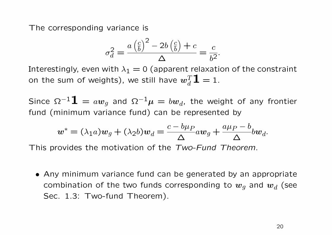
The corresponding variance is

σ2d =

a(

cb

)2 − 2b(

cb

)

+ c

∆=

c

b2.

Interestingly, even with λ1 = 0 (apparent relaxation of the constraint

on the sum of weights), we still have wTd1 = 1.

Since Ω−11 = awg and Ω−1µ = bwd, the weight of any frontier

fund (minimum variance fund) can be represented by

w∗ = (λ1a)wg + (λ2b)wd =

c − bµP

∆awg +

aµP − b

∆bwd.

This provides the motivation of the Two-Fund Theorem.

• Any minimum variance fund can be generated by an appropriate

combination of the two funds corresponding to wg and wd (see

Sec. 1.3: Two-fund Theorem).

20

Feasible set

Given N risky assets, we can form various portfolios from these N

assets. We plot the point (σP , rP ) that represents a particular port-

folio in the σ−r diagram. The collection of these points constitutes

the feasible set or feasible region.

21

Argument to show that the collection of the points representing

(σP , rP ) of a 3-asset portfolio generates a solid region in the σ-r

plane

• Consider a 3-asset portfolio, the various combinations of assets

2 and 3 sweep out a curve between them (the particular curve

taken depends on the correlation coefficient ρ23).

• A combination of assets 2 and 3 (labelled 4) can be combined

with asset 1 to form a curve joining 1 and 4. As 4 moves

between 2 and 3, the family of curves joining 1 and 4 sweep out

a solid region.

22

Properties of the feasible regions

1. For a portfolio with at least 3 risky assets (not perfectly cor-

related and with different means), the feasible set is a solid

two-dimensional region.

2. The feasible region is convex to the left. That is, given any

two points in the region, the straight line connecting them does

not cross the left boundary of the feasible region. This property

must be observed since any combination of two portfolios also

lies in the feasible region. Indeed, the left boundary of a feasible

region is a hyperbola.

23

Locate the efficient and inefficient investment strategies

• Since investors prefer the lowest variance for the same expected

return, they will focus on the set of portfolios with the smallest

variance for a given mean, or the mean-variance frontier.

• The mean-variance frontier can be divided into two parts: an

efficient frontier and an inefficient frontier.

• The efficient part includes the portfolios with the highest mean

for a given variance.

• To find the efficient frontier, we must solve a quadratic pro-

gramming problem.

24

Minimum variance set and efficient funds

The left boundary of a feasible region is called the minimum variance

set. The most left point on the minimum variance set is called the

global minimum variance point. The portfolios in the minimum

variance set are called the frontier funds.

For a given level of risk, only those portfolios on the upper half of

the efficient frontier with a higher return are desired by investors.

They are called the efficient funds.

A portfolio w∗ is said to be mean-variance efficient if there exists

no portfolio w with µP ≥ µ∗P and σ2

P ≤ σ∗2P , except itself. That is,

you cannot find a portfolio that has a higher return and lower risk

than those of an efficient portfolio.

25

6.2 Two-fund Theorem

Take any two frontier funds (portfolios), then any combination of

these two frontier funds remains to be a frontier fund. Indeed, any

frontier portfolio can be duplicated, in terms of mean and variance,

as a combination of these two frontier funds. In other words, all

investors seeking frontier portfolios need only invest in various com-

binations of these two funds.

• In what type of restriction can this property be extended to a

combination of efficient funds (frontier funds that lie on the

upper portion of the efficient frontier)?

26

Proof of the Two-fund Theorem

Let w1 = (w1

1 · · ·w1n), λ

11, λ1

2 and w2 = (w2

1 · · ·w2n)

T , λ21, λ2

2 be two

known solutions to the minimum variance formulation with expected

rates of return µ1P and µ2

P , respectively. Both solutions satisfy

n∑

j=1

σijwj − λ1 − λ2ri = 0, i = 1,2, · · · , n (1)

n∑

i=1

wiri = µP (2)

n∑

i=1

wi = 1. (3)

We would like to show that αw1+(1−α)w2 is a solution corresponds

to the expected rate of return αµ1P + (1 − α)µ2

P .

27

1. The new weight vector αw1+(1−α)w2 is a legitimate portfolio

with weights that sum to one.

2. Check the condition on the expected rate of return

n∑

i=1

[

αw1i + (1 − α)w2

i

]

ri

= αn∑

i=1

w1i ri + (1 − α)

n∑

i=1

w2i ri

= αµ1P + (1 − α)µ2

P .

3. Eq. (1) is satisfied by αw1 + (1 − α)w2 since the system of

equations is linear. The corresponding λ1 and λ2 are given by

λ1 = αλ11 + (1 − α)λ2

1 and λ2 = αλ12 + (1 − α)λ2

2.

4. Given µP , the appropriate portion α is determined by

µP = αµ1P + (1 − α)µ2

P .

28

Global minimum variance portfolio wg and the counterpart wd

For convenience, we choose the two frontier funds to be wg and

wd. To obtain the optimal weight w∗ for a given µP , we solve for α

using αµg +(1−α)µd = µP and w∗ is then given by αw

∗g +(1−α)w∗

d.

Recall µg = b/a and µd = c/b, so α =(c − bµP )a

∆.

Proposition

Any minimum variance portfolio with the target mean µP can be

uniquely decomposed into the sum of two portfolios

w∗P = αwg + (1 − α)wd

where α =c − bµP

∆a.

29

Indeed, any two minimum-variance portfolios wu and wv can be used

to substitute for wg and wd. Suppose

wu = (1 − u)wg + uwd

wv = (1 − v)wg + vwd

we then solve for wg and wd in terms of wu and wv. Recall

w∗P = λ1Ω

−11+ λ2Ω−1

µ

so that

w∗P = λ1awg + (1 − λ1a)wd

=λ1a + v − 1

v − uwu +

1 − u − λ1a

v − uwv,

whose sum of coefficients remains to be 1 and λ1 =c − bµP

∆.

30

Example

Mean, variances, and covariances of the rates of return of 5 risky

assets are listed:

Security covariance, σij mean, ri

1 2.30 0.93 0.62 0.74 −0.23 15.12 0.93 1.40 0.22 0.56 0.26 12.53 0.62 0.22 1.80 0.78 −0.27 14.74 0.74 0.56 0.78 3.40 −0.56 9.025 −0.23 0.26 −0.27 −0.56 2.60 17.68

Recall that w∗ has the following closed form solution

w∗ =

c − bµP

∆Ω−11+

aµP − b

∆Ω−1

µ

= αwg + (1 − α)wd,

where α = (c − bµP )a

∆.

31

We compute w∗g and w

∗d through finding Ω−11 and Ω−1

µ, then

normalize by enforcing the condition that their weights are summed

to one.

1. To find v1 = Ω−11, we solve the system of equations

5∑

j=1

σijv1j = 1, i = 1,2, · · · ,5.

Normalize the component v1i ’s so that they sum to one

w1i =

v1i

∑5j=1 v1

j

.

After normalization, this gives the solution to wg. Why?

32

We first solve for v1 = Ω−11 and later divide v

1 by some constant

k such that 1Tv1/k = 1. We see that k must be equal to a, where

a = 1TΩ−11. Actually, a = 1T

Ω−11 =N∑

j=1

v1j .

2. To find v2 = Ω−1

µ, we solve the system of equations:

5∑

j=1

σijv2j = ri, i = 1,2, · · · ,5.

Normalize v2i ’s to obtain w2

i . After normalization, this gives the

solution to wd. Also, b =N∑

j=1

v2j and c = µ

TΩ−1µ =

N∑

j=1

rjv2j .

33

security v1

v2

wg wd1 0.141 3.652 0.088 0.1582 0.401 3.583 0.251 0.1553 0.452 7.284 0.282 0.3144 0.166 0.874 0.104 0.0385 0.440 7.706 0.275 0.334

mean 14.413 15.202variance 0.625 0.659

standard deviation 0.791 0.812

Recall v1 = Ω−11 and v

2 = Ω−1µ so that

• sum of components in v1 = 1T

Ω−11 = a

• sum of components in v2 = 1T

Ω−1µ = b.

Note that wg = v1/a and wd = v

2/b.

34

Relation between wg and wd

Both wg and wd are frontier funds with

µg =µ

TΩ−11a

=b

aand µd =

µTΩ−1

µ

b=

c

b.

Difference in expected returns = µd − µg =c

b− b

a=

∆

ab> 0.

Also, difference in variances = σ2d − σ2

g =c

b2− 1

a=

∆

ab2> 0.

Since µd > µg and σ2d > σ2

g , wd is an efficient portfolio that lies on

the upper portion of the efficient frontier.

35

How about the covariance of the portfolio returns for any two min-

imum variance portfolios? Write

ruP = w

Tur and rv

P = wTv r

where r = (r1 · · · rN)T . Recall that for the two special efficient

funds, wg and wd, their covariance is given by

σgd = cov(rgP , rd

P ) = cov

N∑

i=1

wgi ri,

N∑

j=1

wdj rj

=N∑

i=1

N∑

j=1

wgi wd

jcov(ri, rj)

= wTg Ωwd =

Ω−11

a

T

Ω

(

Ω−1µ

b

)

=1T

Ω−1µ

ab=

1

asince b = 1T

Ω−1µ.

36

In general, consider two portfolios parametrized by u and v:

wu = (1 − u)wg + uwd and wv = (1 − v)wg + vwd

so that

cov(ruP , rv

P ) = (1 − u)(1 − v)σ2g + uvσ2

d + [u(1 − v) + v(1 − u)]σgd

=(1 − u)(1 − v)

a+

uvc

b2+

u + v − 2uv

a

=1

a+

uv∆

ab2.

For any portfolio wP ,

cov(rg, rP ) = wTg ΩwP =

1TΩ−1ΩwP

a=

1

a= var(rg).

Therefore, we cannot find a portfolio whose return is uncorrelated

with that of the global minimum variance portfolio.

37

6.3 Inclusion of the risk free asset: One-fund Theorem

Consider a portfolio with weight α for the risk free asset and 1 − α

for a risky asset. The risk free asset has the deterministic rate of

return rf . The mean of the expected rate of portfolio return is

rP = αrf + (1 − α)rj (note that rf = rf).

The covariance σfj between the risk free asset and any risky asset

is zero since

E[(rj − rj) (rf − rf)︸ ︷︷ ︸

zero

] = 0.

Therefore, the variance of portfolio return σ2P is

σ2P = α2 σ2

f︸︷︷︸

zero

+(1 − α)2σ2j + 2α(1 − α) σfj

︸︷︷︸

zero

so that

σP = |1 − α|σj.

38

Since both rP and σP are linear functions of α, so (σP , rP ) lies on a

pair line segments in the σ-r diagram.

1. For 0 < α < 1, the points representing (σP , rP ) for varying values

of α lie on the straight line segment joining (0, rf) and (σj, rj).

39

2. If borrowing of the risk free asset is allowed, then α can be

negative. In this case, the line extends beyond the right side of

(σj, rj) (possibly up to infinity).

3. When α > 1, this corresponds to short selling of the risky asset.

In this case, the portfolios are represented by a line with slope

negative to that of the line segment joining (0, rf) and (σj, rj)

(see the lower dotted-dashed line).

• The lower dotted-dashed line can be seen as the mirror image

with respect to the vertical r-axis of the upper solid line segment

that would have been extended beyond the left side of (0, rf).

This is due to the swapping in sign in |1 − α|σj when α > 1.

• The holder bears the same risk, like long holding of the risky

asset, while µP falls below rf . This is highly undesirable for the

holder.

40

Consider a portfolio that starts with N risky assets originally, what

is the impact of the inclusion of a risk free asset on the feasible

region?

Lending and borrowing of the risk free asset is allowed

For each portfolio formed using the N risky assets, the new combi-

nations with the inclusion of the risk free asset trace out the infinite

straight line originating from the risk free point and passing through

the point representing the original portfolio.

The totality of these lines forms an infinite triangular feasible region

bounded by a pair of symmetric lines through the risk free point,

one line is tangent to the original feasible region while the other

line is the mirror image counterpart. The infinite triangular wedge

contains the original feasible region.

41

We consider the more realistic case where rf < µg (a risky portfolio

should demand an expected rate of return high than rf). For rf <b

a,

the upper line of the symmetric double line pair touches the original

feasible region.

The new efficient set is the single straight line on the top of the

new triangular feasible region. This tangent line touches the original

feasible region at a point F , where F lies on the efficient frontier of

the original feasible set.

42

No shorting of the risk free asset (rf < µg)

The line originating from the risk free point cannot be extended

beyond the points in the original feasible region (otherwise entails

borrowing of the risk free asset). The upper half line is extended up

to the tangency point only while the lower half line can be extended

to infinity.

43

One-fund Theorem

Any efficient portfolio (represented by a point on the upper tangent

line) can be expressed as a combination of the risk free asset and

the portfolio (or fund) represented by M .

“There is a single fund M of risky assets such that any efficient

portfolio can be constructed as a combination of the fund M and

the risk free asset.”

The One-fund Theorem is based on the assumptions that

• every investor is a mean-variance optimizer

• they all agree on the probabilistic structure of asset returns

• a unique risk free asset exists.

Then everyone purchases a single fund, which is then called the

market portfolio.

44

The proportion of wealth invested in the risk free asset is 1−N∑

i=1

wi.

Write r as the constant rate of return of the risk free asset.

Modified Lagrangian formulation

minimizeσ2

P

2=

1

2w

TΩw

subject to µTw + (1 −1T

w)r = µP .

Define the Lagrangian: L =1

2w

TΩw + λ[µP − r − (µ − r1)Tw]

∂L

∂wi=

N∑

j=1

σijwj − λ(µi − r) = 0, i = 1,2, · · · , N (1)

∂L

∂λ= 0 giving (µ − r1)T

w = µP − r. (2)

(µ − r1)Tw is interpreted as the weighted sum of the expected

excess rate of return above the risk free rate r.

45

Remark

In the earlier mean-variance model without the risk free asset, we

have

N∑

j=1

wjrj = µP .

However, with the inclusion of the risk free asset, the corresponding

relation is modified to become

N∑

j=1

wj(rj − r) = µP − r.

In the new formulation, we now consider rj − r, which is the excess

expected rate of return above the risk free rate of return r. This is

more convenient since the contribution of the risk free asset to this

excess expected rate of return is zero so that the weight of the risk

free asset becomes immaterial in the new formulation.

46

Solving (1): w∗ = λΩ−1(µ − r1). Substituting into (2)

µP − r = λ(µ − r1)TΩ−1(µ − r1) = λ(c − 2br + ar2).

By eliminating λ, the relation between µP and σP is given by the

following pair of half lines ending at the risk free asset point (0, r)

σ2P = w

∗TΩw

∗ = λ(w∗Tµ − rw∗T

1)

= λ(µP − r) = (µP − r)2/(c − 2br + ar2).

Here, 1λ =

µP − r

σ2P

may be interpreted as the ratio of excess expected

portfolio return above the riskless interest rate to the variance of

portfolio return.

What is the relationship between this pair of half lines and the

frontier boundary of the feasible region of the risky assets plus the

risk free asset?

47

With the inclusion of the risk free asset, the set of minimum variance

portfolios are represented by portfolios on the two half lines

Lup : µP − r = σP

√

ar2 − 2br + c (3a)

Llow : µP − r = −σP

√

ar2 − 2br + c. (3b)

Recall that ar2−2br+ c > 0 for all values of r since ∆ = ac− b2 > 0.

The minimum variance portfolios without the risk free asset lie on

the hyperbola

σ2P =

aµ2P − 2bµP + c

∆.

48

When r < µg =b

a, the upper half line is a tangent to the hyperbola.

The tangency portfolio is the tangent point to the efficient frontier

(upper part of the hyperbolic curve) through the point (0, r).

49

Solution of the tangency portfolio (assuming r <b

a)

The tangency portfolio M is represented by the point (σP,M , µMP ),

and the solution to σP,M and µMP are obtained by solving simultane-

ously

σ2P =

aµ2P − 2bµP + c

∆

µP = r + σP

√

ar2 − 2br + c.

We obtain

µMP =

c − br

b − arand σ2

P,M =ar2 − 2br + c

(b − ar)2.

Once µMP is obtained, the corresponding values for λM and w

∗M are

λM =µM

P − r

c − 2rb + r2a=

1

b − arand

w∗M = λMΩ−1(µ − r1) =

Ω−1(µ − r1)

b − ar.

50

Properties of the tangency portfolio

Recall µg =b

a. When r <

b

a, it can be shown that µM

P > µg. To

prove the claim, we observe(

µMP − b

a

)(b

a− r

)

=

(c − br

b − ar− b

a

)b − ar

a

=c − br

a− b2

a2+

br

a

=ac − b2

a2=

∆

a2> 0,

so we deduce that µMP >

b

a> r.

Also, we can deduce that σP,M > σg as expected. Why?

Both Portfolio M and Portfolio g are portfolios generated by the

universe of risky assets (with no inclusion of the risk free asset),

and g is the global minimum variance portfolio.

51

Properties of the minimum variance portfolios for r < b/a

1. Efficient portfolios

Any portfolio on the upper half line

µP = r + σP

√

ar2 − 2br + c

within the segment FM joining the two points F(0, r) and M

involves long holding of the market portfolio M and the risk free

asset F , while those outside FM involves short selling of the risk

free asset and long holding of the market portfolio.

2. Any portfolio on the lower half line

µP = r − σP

√

ar2 − 2br + c

involves short selling of the market portfolio and investing the

proceeds in the risk free asset. This represents a non-optimal

investment strategy since the investor faces risk but gains no

extra expected return above r.

52

Degenerate case where µg =b

a= r

• What happens when r = b/a? The half lines become

µP = r ± σP

√

c − 2

(b

a

)

b +b2

a= r ± σP

√

∆

a,

which correspond to the asymptotes of the hyperbolic left bound-

ary of the feasible region with risky assets only.

• Under the scenario: r =b

a, efficient funds still lie on the upper

half line, though the tangency portfolio does not exist. Recall

that

w∗ = λΩ−1(µ − r1) so that

1Tw = λ(1T

Ω−1µ − r1T

Ω−11) = λ(b − ra).

53

• When r = b/a,1Tw = 0 as λ is finite. Any minimum variance

portfolio involves investing everything in the risk free asset and

holding a portfolio of risky assets whose weights are summed to

zero.

• The optimal weight vector w∗ equals λΩ−1(µ − r1) and the

multiplier λ is determined by

λ =µP − r

c − 2br + ar2

∣∣∣∣∣r=b/a

=µP − r

c − 2(

ba

)

b + b2a

=a(µP − r)

∆.

54

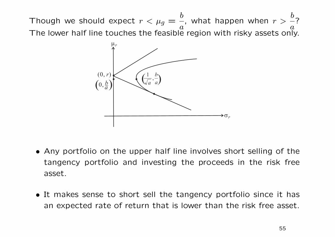
Though we should expect r < µg =b

a, what happen when r >

b

a?

The lower half line touches the feasible region with risky assets only.

• Any portfolio on the upper half line involves short selling of the

tangency portfolio and investing the proceeds in the risk free

asset.

• It makes sense to short sell the tangency portfolio since it has

an expected rate of return that is lower than the risk free asset.

55

Example (5 risky assets and one risk free asset)

Data of the 5 risky assets are given in the earlier example, and

r = 10%.

The system of linear equations to be solved is

5∑

j=1

σijvj = ri − r = 1 × ri − r × 1, i = 1,2, · · · ,5.

Recall that v1 and v

2 in the earlier example are solutions to

5∑

j=1

σijv1j = 1 and

5∑

j=1

σijv2j = ri, respectively.

Hence, vj = v2j − rv1

j , j = 1,2, · · · ,5 (numerically, we take r = 10%).

56

Now, we have obtained v where

v = Ω−1(µ − r1).

Note that the optimal weight vector for the 5 risky assets satisfies

w = λv for some scalar λ.

We determine λ by enforcing (µ − r1)Tw = µP − r, or equivalently,

λ(µ − r1)Tv = µP − r,

where µP is the target rate of return of the portfolio.

The weight of the risk free asset is then given by 1 −5∑

j=1

wj.

57

Interpretation of the tangency portfolio (market portfolio)

• The One-fund Theorem states that everyone purchases a single

fund of risky assets and borrow or lend at the risk free rate.

• If everyone purchases the same fund of risky assets, what must

that fund be? This fund must equal the market portfolio.

• The market portfolio is the summation of all assets. If everyone

buys just one fund, and their purchases add up to the market,

then that fund must be the market as well.

• In the situation where everyone follows the mean-variance method-

ology with the same estimates of parameters, the efficient fund

of risky assets will be the market portfolio.

58

How can this happen? The answer is based on the equilibrium

argument.

• If everyone else (or at least a large number of people) solves the

problem, we do not need to. The return on an asset depends

on both its initial price and its final price. The other investors

solve the mean-variance portfolio problem using their common

estimates, and they place orders in the market to acquire their

portfolios.

• If orders placed do not match with what is available, the prices

must change. The prices of the assets under heavy demand

will increase while the prices of the assets under light demand

will decrease. These price changes affect the estimates of asset

returns directly, and hence investors will recalculate their optimal

portfolio.

59

• This process continues until demand exactly matches supply,

that is, it continues until an equilibrium prevails.

Summary

• In the idealized world, where every investor is a mean-variance

investor and all have the same estimates, everyone buys the

same portfolio and that must be equal to the market portfolio.

• Prices adjust to drive the market to efficiency. Then after other

people have made the adjustments, we can be sure that the

efficient portfolio is the market portfolio.

60

6.4 Addition of a risk tolerance factor

Maximize τµP − σ2P

2, with τ ≥ 0, where τ is the risk tolerance.

Optimization problem: maxw∈RN

τµP − σ2P

2subject to 1T

w = 1.

• Instead of only minimizing risk as in the mean variance mod-

els, the new objective function represents the tradeoff between

return and risk with weighted factor 2τ . When τ is high, the

investor is more interested in expected return and has a high

tolerance on risk.

• The tolerance factor τ is chosen by the investor and will be

fixed in the formulation. The choice variables are the portfolio

weights wi, i = 1,2, · · · , N .

• The parameter τ is closely related to the relative risk aversion

coefficient. Given an initial wealth W0 and under a portfolio

choice w, the end-of-period wealth is W0(1 + rP ).

61

Write µP = E[rP ] and σ2P = var(rP ), and let u denote the utility

function.

Consider the Taylor expansion of the terminal utility value

u[W0(1 + rP )] ≈ u(W0) + W0u′(W0)rP +W2

0

2u′′(W0)r

2P + · · · .

Neglecting the third and higher order moments and noting E[r2P ] =

σ2P + µ2

P .

Next, considering the expected utility value of the terminal wealth

E[u(W0(1 + µP ))] ≈ u(W0) + W0u′(W0)µP +W2

0

2u′′(W0)(σ

2P + µ2

P ) + · · ·

= u(W0) − W20 u′′(W0)

[

− u′(W0)

W0u′′(W0)µP − σ2

P + µ2P

2

]

+ · · ·

62

Neglecting µ2P compared to σ2

P and recalling RR = −W0u′′(W0)

u′(W0)as

the relative risk aversion coefficient, we obtain the objective func-

tion:1

RRµP − σ2

P

2. The deterministic multiplier −W0u′′(W0)

u′(W0)is pos-

itive since u′(W0) > 0 and u′′(W0) < 0. The constant u(W0) in the

expected utility value are immaterial. Lower relative risk aversion

means higher risk tolerance.

The expected utility can be expressed solely in terms of mean µP

and variance σ2P when

(i) u is a quadratic function [u′′′(W0) and higher order derivatives

do not appear], or

(ii) rP is normal (third and higher order moments become irrelevant

statistics).

63

Quadratic optimization problem

maxw∈RN

[

τµTw − w

TΩw

2

]

subject to wT1 = 1.

The Lagrangian formulation becomes:

L(w;λ) = τµTw − w

TΩw

2+ λ(wT1− 1).

The first order conditions are

τµ − Ωw∗ + λ1 = 0

w∗T1 = 1

.

When τ is taken to be zero, the problem reduces to the minimization

of portfolio return variance without regard to expected portfolio

return. This gives the global minimum variance portfolio w∗g.

64

Express the optimal solution w∗ as wg + τz

∗, τ ≥ 0.

1. When τ = 0, the two first order conditions become

Ωw = λ01 and 1Twg = 1.

Solving

wg = λ0Ω−11 and 1 = 1T

wg = λ01TΩ−11

hence

wg =Ω−11

1TΩ−11

(independent of µ).

The formulation does not depend on µ when τ is taken to be

zero.

65

2. When τ ≥ 0, we obtain w = τΩ−1µ + λΩ−11. To determine λ,

we apply

1 = 1Tw = τ1T

Ω−1µ + λ1T

Ω−11 so that λ =1 − τ1Ω−1

µ

1TΩ−11

.

w∗ = τΩ−1

µ +1 − τ1T

Ω−1µ

1TΩ−11

Ω−11

= τ

Ω−1µ − 1T

Ω−1µ

1TΩ−11

Ω−11

+ wg.

We obtain w∗ = wg + τz

∗, where

z∗ = Ω−1

µ − 1TΩ−1

µ

1TΩ−11

Ω−11 and 1Tz∗ = 0.

Write rwg as the random rate of return of portfolio g, and a

similar notation for z∗. Observe that cov(rwg, rz∗) = z

∗TΩwg =

0,

µz∗ = µTz∗ = c − b2

a=

∆

a> 0 and σ2

z∗ =∆

a> 0.

66

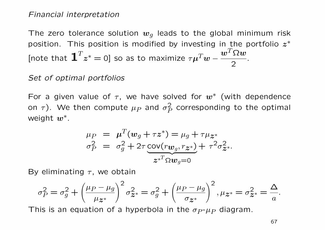
Financial interpretation

The zero tolerance solution wg leads to the global minimum risk

position. This position is modified by investing in the portfolio z∗

[note that 1Tz∗ = 0] so as to maximize τµ

Tw − w

TΩw

2.

Set of optimal portfolios

For a given value of τ , we have solved for w∗ (with dependence

on τ). We then compute µP and σ2P corresponding to the optimal

weight w∗.

µP = µT(wg + τz

∗) = µg + τµz∗

σ2P = σ2

g + 2τ cov(rwg, rz∗)︸ ︷︷ ︸

z∗T Ωwg=0

+ τ2σ2z∗.

By eliminating τ , we obtain

σ2P = σ2

g +

(

µP − µg

µz∗

)2

σ2z∗ = σ2

g +

(

µP − µg

σz∗

)2

, µz∗ = σ2z∗ =

∆

a.

This is an equation of a hyperbola in the σP -µP diagram.

67

µP = ba + ∆

a τ

σ2P = 1

a + ∆a τ2

The points representing these optimal portfolios in the σP -µP dia-

gram lie on the upper half of the hyperbola. We expect that for a

higher value of τ chosen by the investor, the optimal portfolio has

higher µP and σP .

68

How to reconcile the mean-variance model and risk-tolerance

model?

Recall that the left boundary of the feasible region of the risky assets

is given by

σ2P =

aµ2P − 2bµP + c

∆, ∆ = ac − b2. (1)

The parabolic curve that traces all optimal portfolios of the risk-

tolerance model in the σ2P -µP diagram is

µP =b

a+

∆

aτ and σ2

P =1

a+

∆

aτ2. (2)

It can be shown that the solutions to µP and σ2P in Eq. (2) satisfy

the parabolic equation (1) since

σ2P =

a(

ba + ∆

a τ)2 − 2b

(ba + ∆

a τ)

+ c

∆=

1

a+

∆

aτ2.

69

With a given tolerance τ , the objective function line

τµP − σ2P

2= constant

is pushed upwards until it becomes the tangent line to the parabolic

curve.

2

p

P

2

p =a 2b + c P P

2

PP

2

2= constant

70

• The objective function line: τµP − σ2P

2= constant in the σ2

P -µP

diagram is pushed upwards as much as possible in the maximiza-

tion procedure.

• However, the optimal portfolio must lie in the feasible region of

risky assets. Recall that the feasible region is bounded on the

left by the parabolic curve: σ2P =

aµ2P − 2bµP + c

∆. The objective

function τµP − σ2P

2is maximized when the objective function line

touches the left boundary of the feasible region.

• In the degenerate case τ = 0, the slope of the line: τµP − σ2P2 =

constant becomes infinite. When we maximize −σ2P2 = constant

by pushing the vertical line to the far left, the corresponding

optimal portfolio obtained is Portfolio g.

71

Another version of the Two-fund Theorem

Given µP , the efficient fund under the mean-variance model is given

by

w∗ = w

∗g +

a

∆

(

µP − b

a

)

z∗, µP > µg =

b

a,

where w∗g =

Ω−11a

, z∗ = Ω−1µ − b

aΩ−11.

This implies that any efficient fund can be generated by the two

funds: global minimum variance fund w∗g and the fund z

∗.

72

Proof

1. Note that w∗ is of the form λ1Ω

−11+ λ2Ω−1

µ.

2. Consider the expected portfolio return:

µTw

∗ = µg +a

∆

(

µP − b

a

)

µz∗ =b

a+

a

∆

(

µP − b

a

)∆

a= µP .

3. Consider the sum of weights:

1Tw

∗ = 1Tw

∗g +

a

∆

(

µP − b

a

)

1Tz∗ = 1.

73

Comparing the first order conditions of the mean-variance model

and risk-tolerance model

1. Ωw∗ = λ11+ λ2µ 2. Ωw

∗ = λ1+ τµ

1Tw

∗ = 1 1Tw

∗ = 1

1Tµ = µP

We observe that

λ1 = λ =c − bµP

∆

λ2 =aµP − b

∆is simply τ.

The specification of risk tolerance τ is somewhat equivalent to the

specification of µP .

74

Summary

1. The objective function τµTw − w

TΩw

2represents a balance of

maximizing return τµTw against risk

wTΩw

2, where the weighing

factor τ is related to the reciprocal of the relative risk aversion

coefficient RR.

2. The optimal solution takes the form

w∗ = wg + τz

∗

where wg is the portfolio weight of the global minimum variance

portfolio and the weights in z∗ are summed to zero.

75

Note that

z∗ = Ω−1

µ − b

aΩ−11 = b(wd − wg).

Alternatively,

w∗ = wg +

ab

∆

(

µP − b

a

)

(wd − wg)

and τ and µP are related by

τ =a

∆

(

µP − b

a

)

.

76

3. The additional variance above σ2g is given by

τ2σ2z∗ = τ2∆

a, ∆ = ac − b2.

Also, cov(rwg, rz∗) = 0, that is, rwg and rz∗ are uncorrelated

4. The efficient frontier of the mean-variance model coincides with

the set of optimal portfolios of the risk-tolerance model. The

risk tolerance τ and expected portfolio return µP are related by

µP − µg

µz∗=

µP − µg

σ2z∗

= τ.

5. A new version of the Two-fund Theorem can be established

where any efficient fund can be generated by the two funds: w∗g

and z∗.

77

6.5 Asset-liability model

Liabilities of a pension fund = future benefits − future contributions

Market value can hardly be determined since liabilities are not read-

ily marketable, unlike tradeable assets. Assume that some specific

accounting rules are used to calculate an initial value L0. If the

same rule is applied one period later, a value for L1 results. Note

that L1 is random.

Rate of growth of the liabilities = rL =L1 − L0

L0, where rL is ex-

pected to depend on the changes of interest rate structure, mortality

and other stochastic factors.

Let A0 be the initial value of assets. The investment strategy of

the pension fund is given by the portfolio choice w. Let rw denote

the rate of growth of the asset portfolio.

78

Surplus optimization

Depending on the portfolio choice w, the surplus gain after one

period

S1 − S0 = [A0(1 + rw) − L0(1 + rL)] − (A0 − L0) = A0rw − L0rL.

The rate of return on the surplus is defined by

rS =S1 − S0

A0= rw − 1

f0rL

where f0 = A0/L0 is the initial funding ratio. Here, rS is the differ-

ence of two random variables: rw and 1f0

rL, one of them is depen-

dent on the choice variable w while the other is not.

79

Maximization formulation

maxw∈RN

τE

[

rw − 1

f0rL

]

− 1

2var

(

rw − 1

f0rL

)

subject toN∑

i=1

wi = 1. Since E

[

1

f0rL

]

and var(rL) are independent

of w so that they can be omitted from the objective function.

We rewrite the quadratic maximization formulation as

maxw∈RN

τE[rw] − var(rw)

2+

1

f0cov(rw, rL)

subject toN∑

i=1

wi = 1. Recall that

cov(rw, rL) = cov

N∑

i=1

wiri, rL

=N∑

i=1

wicov(ri, rL).

80

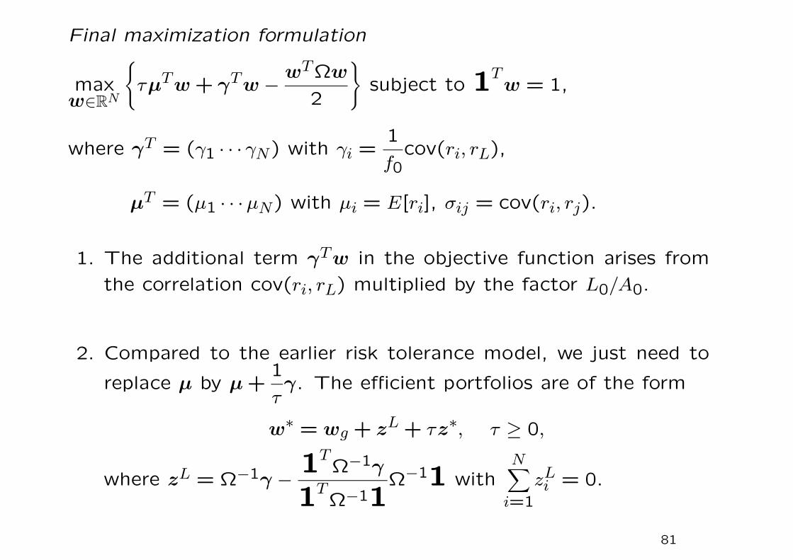
Final maximization formulation

maxw∈RN

τµTw + γ

Tw − w

TΩw

2

subject to 1Tw = 1,

where γT = (γ1 · · · γN) with γi =

1

f0cov(ri, rL),

µT = (µ1 · · ·µN) with µi = E[ri], σij = cov(ri, rj).

1. The additional term γTw in the objective function arises from

the correlation cov(ri, rL) multiplied by the factor L0/A0.

2. Compared to the earlier risk tolerance model, we just need to

replace µ by µ +1

τγ. The efficient portfolios are of the form

w∗ = wg + z

L + τz∗, τ ≥ 0,

where zL = Ω−1

γ − 1TΩ−1

γ

1TΩ−11

Ω−11 withN∑

i=1

zLi = 0.

81