mathematica aeterna, vol. 7, 2017, no. 1, 1 - 17 · 1department of applied science, rcciit,...

DYNAMICS OF FRACTIONAL ORDER CHAOTIC SYSTEM

M. Jana11Department of Applied Science, RCCIIT, Beliaghata, Kolkata-700015 [email protected]

M. Islam2

2Department of Mathematics, Indian Statistical Institute, Kolkata-700108 [email protected]

N. Islam3

3Department of Mathematics, Ramakrishna Mission Residential College, NarendrapurKolkata-700146 [email protected]

H.P. Mazumdar44Department of Physics and Applied Mathematics, Indian Statistical Institute, Kolkata-700108

[email protected]

Abstract

This paper deals with the dynamics of chaos and synchronization for fractional order chaotic system. For fractionalorder derivative Captuo definition is used here and numerical simulations are done using Predictor-Correctorsscheme by Diethlm based on the Adams-Baseforth-Moulton algorithm. Stability analysis is discussed here fornon linear fractional order chaotic system and synchronization is achieved between two non identical fractionalorder chaotic systems: Finance chaotic system(driving system)and Lorenz system(response system)via activecontrol.Numerical simulations are performed to show the effectiveness of these approaches.

Key words: Fractional calculus;Chaos;Bifurcation; Non linear finance chaotic system; Lorenz chaotic sys-tem;stability;Synchronization;Active control technique.

MSC 2010 : 34D06, 34D23

1. Introduction

As the wide ranging applications of chaos and synchronization became increasingly clear over the past few decades,the research community witnessed much activity in the areas of chaos control and synchronization. Several papershave been published on chaos control and synchronization by mathematicians, engineers and physicists. Pecoraand Carroll [1] first gave the new dimension to the chaos synchronization for integer order system. After thatmany types of synchronization such as adaptive control, active control, time delayed control, feedback controletc. [2]-[5] have been adopted in this literature. However, the motivating problems and examples in these areashave exclusively been integer order dynamical systems.

On the other hand, the last few decades witnessed a resurrection of the three hundred year old subject of fractionalcalculus. Using fractional calculus (FC), it is possible to depict many physical problems using mathematical mod-els, that have been impossible within the ambit of classical calculus. In particular, the problems which exhibitsthe property of memory (time or location or both), for example diffusion process in non uniform medium haveelegant description in terms of fractional calculus. Thus the generalization of classical calculus with the help offractional calculus enhances the reach and power of calculus. As a result, it has been applied in control theory[6]-[7], viscoelasticity [8], diffusion [9], electromagnetism [10], signal processing [11]-[12] and bio engineering [13]-[14].A theory on controlling a fractional order system can be thought of as a useful generalization of the traditionalcontrol theory. The same is true for synchronization of fractional order chaotic systems. In the recent years,some important research has been conducted at the interface of chaos theory and fractional calculus. Variousauthors have worked on the stability, chaos and control of chaos on popular fractional order chaotic systems suchas the Lorentz system [15], Chen system [16], Rossler system [17], Newton-Leipnic system [18] and Liu system [19].

In this paper, our target is to analyze the synchronization phenomenon between two different fractional orderchaotic systems. This abstract formulation has important applications in secure communication using chaos.We motivate the discussion by comparing the dynamics of nonlinear fractional order system with that of thecorresponding integer order system. The paper has been arranged as follows. Section 2 recapitulates the basic

Mathematica Aeterna, Vol. 7, 2017, no. 1, 1 - 17

2 DYNAMICS OF FRACTIONAL ORDER CHAOTIC SYSTEM

ideas of fractional calculus. Section 3 describes the stability analysis of chaos for integer order chaotic systemwhile Section 4 discusses the same for fractional order chaotic system. In Section 5, the fractional order systemis stabilized at its equilibrium points using feedback control. Synchronization is achieved between the fractionalorder non linear finance chaotic system and fractional order Lorentz system using active control method in Section6. The range of the system parameters for the non linear fractional order finance system. Numerical simulationsare carried in Section 7 to illustrate these theoretical results. The appendix summarizes the numerical algorithmused for solving fractional order differential equations.

2. Basics of Fractional calculus

The idea of “Fractional calculus”at first came to the knowledge of L-Hospital in 1695. In “Fractional calculus”,the generalized operator “differenintegral”was introduced which is now denoted by aD

qt , where a and t are bounds

of the operator with q as order for any real number. It is also naively written as aDqt (f) =

dqf(t)

d(t− a)q. However, the

most used definitions of differenintegral operator are the definitions proposed by Riemann- Liouville, Grunwald-Letnikov and Caputo. Weyl, Fourier, Cauchy and Abel, among many others, had also proposed other definitionsfor such operators. The three most widely used definitions are as follows :

Definition 1. The three equivalent definitions of fractional order derivatives are as follows :

(1) Grunwald-Letnikov definition

aDqt (f) = lim

N→∞

[t− aN

]−q N−1∑j=0

(−1)j(q)f(t− j[t− aN

])

(2) Riemann-Liouville definition

aDqt (f) =

1

Γ(n− q)dn

dtn

∫ t

a

f(τ)

(t− τ)q−n+1 dτ, for n− 1 < q < n.

(3) Caputo definition

aDqt (f) =

1

Γ(n− q)

∫ t

a

fn(τ)

(t− τ)q−n+1 dτ, for n− 1 < q < n.

The Laplace transform of Riemann-Liouville fractional derivative is

L {aDqt }(f) = sqL f(t)−

n−1∑k=0

skD(q−k−1)f(0)

and that of Caputo’s fractional derivative is

L {aDqt (f)}sqL {f(t)} −

n−1∑k=0

s(q−k−1)f (k)(0).

It is seen that the Laplace transform of fractional order derivative for Caputo’s definition does not require anyinitial condition involving fractional order derivatives, although it is necessary for Riemann’s definition. As mostof the physical problems have initial conditions with integer order derivatives only, it is more convenient to useCaputo’s definition in mathematical models involving fractional calculus.

Using Riemann-Liouville definition, we find that the derivative of a constant c is ct−α

Γ(1−α)where as by Caputo’s

definition it is zero. Thus, Caputo’s defintion treats fractional differentiation as a generalization of the classicalineteger order differentiation. Thus it is more convenient to use Caputo’s definition while modelling real worldproblems using fractional order differential equations. Hence, in this paper, we use Caputo’s definition of fractionalorder derivatives.

3. Chaos and stability analysis of integer order chaotic system

In order to discuss the stability of a fractional order chaotic system, it is instructive to begin with the corre-sponding integer order system. Let us consider the non linear finance chaotic system as an example, which isgiven by

(1)

x1 = x3 + (x2 − a)x1

x2 = 1− bx2 − x21

x3 = −x1 − cx3

The system (1) exhibits chaos for two sets of parameter values {a = 3.6, b = 0.1, c = 1.0} and {a = 0.00001, b =0.1, c = 1.0}.

DYNAMICS OF FRACTIONAL ORDER CHAOTIC SYSTEM 3

The system (1) admits three equilibrium points

E1(0, 1b, 0)

E2(√

c−b−abcc

, 1+acc,− 1

c

√c−b−abc

c)

E3(−√

c−b−abcc

, 1+acc, 1c

√c−b−abc

c)

assuming the conditions (c − b − abc) ≥ 0 with b, c 6= 0 on the parameters. The Jacobian matrix for the abovesystem of equations computed at the point P (x1, x2, x3) is

J =

x2 − a x1 1−2x1 −b 0−1 0 −c

To study the stability of the system at the equilibrium point Ei, we consider the characteristic equation ofthe Jacobian matrix J at Ei. We choose the above said sets of parameter values {a = 3.6, b = 0.1, c = 1.0} and{a = 0.00001, b = 0.1, c = 1.0} for which the system is chaotic.

3.1. Case 1. For the first set of parameter values {a = 3.6, b = 0.1, c = 1.0} , the equilibrium points areE1(0, 10, 0),E2(0.7348, 4.6,−0.7348) and E3(−0.7348, 4.6, 0.7348).

The eigenvalues at the equilibrium point E1(0, 10, 0) are λ1 = −0.1, λ2 = −0.8623 and λ3 = 6.2623 whichindicates that the equilibrium point E1 is a saddle point and unstable.

At E2 and E3, the Jacobian matrix have the eigenvalues λ1 = −0.7123, λ2 = 0.3062 + 1.1927i and λ3 =0.3062− 1.1927i, implying that the equilibrium points are saddle focus and unstable.

3.2. Case 2. For the second set of parameter values {a = 0.00001, b = 0.1, c = 1.0}, the equilibrium points areE1(0, 10, 0), E2(0.94868, 1.00001,−0.94868) and E3(−0.94868, 1.00001, 0.94868).

The eigenvalues at the equilibrium point E1(0, 10, 0) are λ1 = 9.9083, λ2 = −0.9083 and λ3 = −0.1 whichindicates that the equilibrium point E1 is a saddle point and unstable.

At E2 and E3, the Jacobian matrix have the eigenvalues λ1 = −0.7749, λ2 = 0.3374 + 1.4863i and λ3 =0.3374− 1.4863i, implying that the equilibrium points are saddle focus and unstable.

4. Chaos and stability analysis of fractional order chaotic system

Now consider the fractional order non linear finance chaotic system which is described by

(2)

dq1x1

dtq1

= x3 + (x2 − a)x1

dq2x2

dtq2

= 1− bx2 − x21

dq3x3

dtq3

= −x1 − cx3

As before same sets of parameter values {a = 3.6, b = 0.1, c = 1.0} and {a = 0.00001, b = 0.1, c = 1.0} areconsidered here for discussion and studied case wise.

The equilibrium points of the above fractional order system are same as integer order chaotic system and for thiscase we denote them as E∗

i(i = 1, 2, 3)

The stability region of the fractional order system is enhanced using lemma [21]-[23] for fractional order systems.

Lemma 2. If the eigenvalues of the Jacobian matrix (for fractional order system)satisfy |arg(λ)| ≥ π q2,where q =

q1 = q2 = q3 then the system is asymptotically stable at the equilibrium points.


4.1. Case 1. For the parameter values a = 3.6, b = 0.1 and c = 1, the equilibrium points are E∗1(0, 10, 0),

E∗2(0.7348, 4.6,−0.7348) and E∗

3(−0.7348, 4.6, 0.7348) same as integer order chaotic system.

Result 3. The equilibrium point E∗1

is unstable for any q ∈ (0, 1).

Proof. The eigenvalues of the Jacobian matrix for the fractional order financial system at the equilibrium pointE∗

1are λ1 = 6.2623,λ2 = −0.8623 and λ3 = −0.1. Since one of the eigenvalues is positive real number, the

equilibrium point E∗1

could not be stabled for any q ∈ (0, 1). �

Result 4. The equilibrium points E∗2

and E∗3

are stable for any q < 0.84.

Proof. The eigenvalues of the Jacobian matrix for the fractional order financial system at the equilibrium pointsE∗

2and E∗

3are λ1 = −0.7123, λ2 = 0.3062 + 1.1927i and λ3 = 0.3062− 1.1927i.Though the complex eigenvalues

have the positive real part, according to the above Lemma the equilibrium points are controllable for

|arg(λ1 , λ2 , λ3)| > πq

2i.e. q < 0.84

Thus the fractional order financial system is stable at the equilibrium points E∗2

and E∗3

for any q < 0.84. �

4.2. Case 2. For the parameter values a = 0.00001, b = 0.1 and c = 1, the equilibrium points are E∗1(0, 10, 0),

E∗2(0.9487, 1.00001,−0.9487) and E∗

3(−0.9487, 1.00001, 0.9487)


is unstable for any q ∈ (0, 1).

Proof. The eigenvalues of the Jacobian matrix for the fractional order financial system at the equilibrium pointE∗

1are 9.9083,-0.9083,-0.1. Since one of the eigenvalues is positive real number, the equilibrium point E∗

1could

not be stabled for any q ∈ (0, 1). �


and E∗3

are stable for any q < 0.85.

Proof. The eigenvalues of the Jacobian matrix for the fractional order financial system at the equilibrium pointsE∗

2and E∗

3are λ1 = −0.7749, λ2 = 0.3374 + 1.4863i and λ3 = 0.3374− 1.4863i.Though the complex eigenvalues

have the positive real part, according to the above Lemma the equilibrium points are controllable for

|arg(λ1 , λ2 , λ3)| > πq

2i.e. q < 0.8578

Thus the fractional order financial system is stable at the equilibrium points E∗2

and E∗3

for any q < 0.85. �

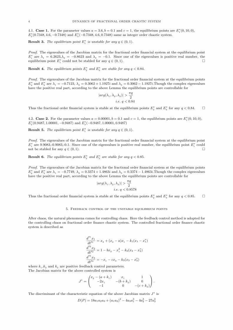
5. Feedback control of the unstable equilibrium points

After chaos, the natural phenomena comes for controlling chaos. Here the feedback control method is adopted forthe controlling chaos on fractional order finance chaotic system. The controlled fractional order finance chaoticsystem is described as

dq1x1

dtq1

= x3 + (x2 − a)x1 − k1(x1 − x∗1)

dq2x2

dtq2

= 1− bx2 − x21− k2(x2 − x∗2)

dq3x3

dtq3

= −x1 − cx3 − k3(x3 − x∗3)

where k1 ,k2 and k3 are positive feedback control parameters.The Jacobian matrix for the above controlled system is

J∗ =

x2 − (a+ k1) x1 1−2x1 −(b+ k2) 0−1 0 −(c+ k3)

.

The discriminant of the characteristic equation of the above Jacobian matrix J∗ is

D(P ) = 18a1a2a3 + (a1a2)2 − 4a3a31 − 4a3

2 − 27a23


where a1 ,a2 and a3 are given by

a1 = a+ b+ c+ k1 + k2 + k3 − x∗2a2 = −bx∗2 − k2x

∗2 + ab+ ak2 + bk1 + k1k2 + 2x∗1

2+ bc+ bk3 + ck2 + k2k3

− cx∗2 − k3x∗2 + ac+ ak3 + ck1 + k1k3 + 1

a3 = (a+ k1 − x∗2)(bc+ bk3 + ck2 + k2k3) + 2x∗12(c+ k3) + (b+ k2)

We choose k1 = k2 = k3 = α and term α as the feedback control parameter.

Routh-Hurwitz criteria for fractional order system:If P (λ) = λ3 + a1λ

2 + a2λ+ a3 be the characteristic polynomial of the Jacobian matrix at the equilibrium pointof the fractional order system and the discriminant be

D(P ) = 18a1a2a3 + (a1a2)2 − 4a3a31 − 4a3

2 − 27a23

then the following conditions hold.[24]-[25]

i) The necessary and sufficient condition that the corresponding equilibrium point of the fractional ordersystem is locally asymptotically stable if D(P ) > 0 and a1 > 0, a3 > 0, a1a2 − a3 > 0.

ii) If D(P ) < 0, and a1 > 0, a2 > 0, a3 > 0 the corresponding equilibrium point of the fractional ordersystem is locally asymptotically stable for q < 2

3.

(iii) If D(P ) < 0, and a1 < 0, a2 < 0 the corresponding equilibrium point of the fractional order system islocally asymptotically stable for q > 2

3.

(iv) If D(P ) < 0, and a1 > 0, a2 > 0, a1a2−a3 = 0, then the corresponding equilibrium point of the fractionalorder system is locally asymptotically stable for q ∈ [0, 1).

(v) a3 > 0 is the necessary condition for the stability of the corresponding equilibrium point of the fractionalorder system.

5.1. Case 1. For the set of parameter values a = 3.6, b = 0.1 and c = 1.0, the results are discussed here.

Result 7. For the feedback control parameter α > 10, the equilibrium point E∗1(0, 10, 0) is stable for any fractional

order q.

Proof. If we choose the feedback control parameter α > 10, we see a1 > 0,a2 > 0, a3 > 0 and the discriminantD(p) of the characteristic equation for the controlled financial chaotic system is also positive. Consequently theequilibrium point E∗

1can be stabilized for any fractional order q using Routh-Hurwitz criteria for fractional order

system. �

Result 8. The equilibrium points E∗2(0.7348, 4.6,−0.7348) and E∗

3(−0.7348, 4.6, 0.7348) are stable for q < 2

3for

feedback control parameter α > 0.

Proof. As the coefficients a1 , a2 and a3 are all positive and the discriminant D(p) is negative when α > 0, Theequilibrium points E∗

2and E∗

3are controllable with q < 2

3by Routh-Hurwitz criteria. �


and E∗3

are stable for any q ∈ (0, 1) with feedback control parameter α = 0.3.

Proof. When k1 = k2 = k3 = α = 0.3,the discriminant D(p) of the characteristic equation is negative whereasa1 , a2 > 0 and a1a2 − a3 = 0. By Routh-Hurwitz criteria the equilibrium points E∗

2and E∗

3become stable for

any q ∈ (0, 1). �

5.2. Case 2. In this case we study the control analysis with the parameter values a = 0.00001, b = 0.1, c = 1.0


is stable for any fractional order q with feedback control parameter α > 11.

Proof. If α > 11, the coefficients of the characteristic equation of the Jacobian matrix for the controlled financechaotic system a1 > 0,a2 > 0 and a3 > 0 and the discriminant D(p) of the characteristic equation is also positive.By Routh-Hurwitz criteria, the equilibrium point E∗

1is stable for any fractional order q. �


and E∗3

are stable for q < 23

for feedback control parameter α > 0.


Proof. The coefficients of the characteristic equation of the Jacobian matrix for the controlled finance chaoticsystem a1 ,a2 , a3 are all positive and the discriminant D(p) is negative when α > 0. By Routh-Hurwitz criteria,the equilibrium points E∗

2and E∗

3are stable for q < 2

3. �


and E∗3

are stable for any q ∈ (0, 1) with feedback control parameterα = 0.335. .

Proof. When k1 = k2 = k3 = α = 0.335,the discriminant D(p) of the characteristic equation is negative whereasa1 , a2 > 0 and a1a2 − a3 = 0. By Routh-Hurwitz criteria the equilibrium point E∗

2and E∗

3become stable for

any q ∈ (0, 1). �

5.3. Numerical Investigation of the feedback control problem: In this section, we numerically investigateseveral aspects of the feedback control problem which are difficult to address through theoretical computations.The two main questions that will be discussed here are :

(i) Determination of a critical value for the control parameter α, that is, a critical value below which thefeedback controller is ineffective

(ii) Relation between the control parameter α and the order of the fractional order derivative q

We first work with Case 1. In figure 1, we address our question (i). It plots bifurcation diagram of the feedbackcontrolled finance chaotic system of order q = 0.98. The diagram proves the existence of a critical control factorα0 around 0.25. The figure clearly illustrates the transition to asymptotic stability as α increases past α0 (referto Section 5.1). Figures 2(a) and (b) present the local behaviour of the system around E∗

2 in the absence andpresence of feedback control. The two variable bifurcation diagram (figure 3) with respect to the feedback controlparameter α and fractional order of the system q explores our question (ii). The blue region of this diagram is theset of α− q values for which the finance system remains stable. The red region represents the respective valuesfor which the system approaches a high periodic orbit or becomes chaotic. The intermediate colours indicatea transition from stability towards chaos through period-doubling bifurcation. The gradient of the colour fromblue towards red indicates an increase in periodicity. It is observable that for lower values of q, the system hasa greater tendency to stabilize - relatively small value of the control parameter α stabilizes the system in thissituation. For values of q close to 1, the system does not stabilize inspite of large values of α. This numericalcomputation indicates a complex relationship that exists between α and q.

Now we work with Case 2. Figure 4 illustrates the existence of a critical feedback control parameter α∗0 close

to 0.25 (like in Case 1) and answers question (i). Thus, the change of the parameter set (a, b, c) does not havea marked effect on the critical value of the control parameter. Figures 5 and 6 illustrate the local behaviourof the finance system around the equilibrium points E∗

2 and E∗3 both in presence and absence of the feedback

controllers. Figure 7, the two variable bifurcation diagram between α and q, seeks the answer to (ii). As in theprevious discussion for case 1, here also blue regions indicate stability, red and dark red regions indicate chaoticand high periodic behaviour while the light blue, green, yellow and orange indicate a increase in periodicity (thecolours have been named in the increasing order of periodicity). This figure indicates a marked change from whatwas observed for Case 1. Here we restricted α between 0 and 0.1 while q was larger than 0.8. It was observedthat whatever be the value of q, depending on the value of α, the stability behaviour keeps switching. As αis varying in a range that lies below the critical coupling α∗

0, one has no reason to expect stable regions. Butthen, the numerical investigation suggests the existence of certain very narrow windows for the values of α whichstabilizes the system inspite of lying below the critical value. We believe that the existence of these windows isreminiscent of the stable windows arising in the bifurcation diagram of chaotic systems and implies a complexdependence of the system dynamics on α and q.

6. Synchronization of fractional order chaotic systems

The classical synchronization problem considered by Pecorra and Carroll [1] involved two identical systems whichwhen coupled through a weak, diffusive coupling, ended up being in perfect synchrony although the originalsystems might have been chaotic themselves. This spontaneous appearance of apparent order in a pair of chaoticsystems arising out of the simple diffusive coupling is perhaps the most fascinating aspect of chaos synchronization.

6.1. Synchronization of structurally equivalent systems with parameter mismatch: Let us considera pair of structurally equivalent systems (X,Y ) with parameter mismatch. In the following, we will denote the

original parameter by θ ∈ Rn and the mismatched parameter by θ ∈ Rn. The pair of structurally equivalentsystems with parameter mismatch can then be represented by

(3)Dq

X = f(X) + g(X)θ

Dq

Y = f(Y ) + g(Y )θ


where Dq

≡

Dq1

Dq2

...

Dqn

and D ≡ ddt.

We consider the fractional order nonlinear finance system as Dq1x1

Dq2x2

Dq3x3

=

x3 + x2x1

1− x12

−x1

+

−x1 0 00 −x2 00 0 −x3

abc

,

that is,

Dq

X = f(X) + g(X)θ,

which is the master system and the corresponding slave system is

Dq

Y = f(Y ) + g(Y )θ.

Here X =

x1x2x3

, Y =

y1y2y3

, f(X) =

x3 + x2x11− x12−x1

, g(X) =

−x1 0 00 −x2 00 0 −x3

, θ = abc

, θ =

abc

.

We will design a suitable control input to bring about a synchronization of the pair (X,Y ) with X as themaster and Y as the slave system. In order to achieve this, we introduce a external force input U(X,Y )to the slave system.

Theorem 13. For the control input

U(X,Y ) = g(Y )θ − g(X)θ − k(Y −X),

there exists a diffusive coupling factor k > k0 = max{2M − (a+ a),M − (b+ b)} such that the systemsX and Y attain globally stable synchronization.

Proof. Let us define the synchronization error as e = Y −X. Then, with the form of U(X,Y ) as in thetheorem, the error dynamics of the coupled system becomes D

q1e1

Dq2e2

Dq3e3

=(f(Y )− f(X)) + (g(Y )− g(X))(θ + θ)− k(Y −X)

=

y2 − (a+ a+ k) x1 1

−(x1 + y1) −(b+ b+ k) 0−1 0 0

e1e2e3

= Q

e1e2e3

where Q =

y2 − (a+ a+ k) x1 1

−(x1 + y1) −(b+ b+ k) 0−1 0 −(c+ c+ k)

If λ is an eigenvalue of the matrix Q and the eigenvector corresponding to this λ is ω = (ω1, ω2, ω3)T ,then

Qω = λω

It is clear that the eigenvalues are functions of time as the matrix Q is a function of the state variables.We emphasize this by rewriting the above equation as,

(4) Q(t)ω(t) = λ(t)ω(t)

Let QH denote the conjugate transpose of the matrix Q. Then, we have,

(5) ω(t)H Q(t) +Q(t)H

2ω(t) =

1

2(λ(t) + λ(t))(ω(t)

H

ω(t))


We know that the chaotic attractor is a compact set. So, any continuous function defined on the chaoticattractor will be bounded. Restricting our discussion to the chaotic trajectories of the finance system,we can thus find a constant M ∈ R such that ||X(t)||∞ ≤M and ||Y (t)||∞ ≤M for all t ∈ R. Here, weuse the notation ||X||∞ for the uniform norm in Rl, that is, ||X||∞ = max1≤i≤lXi.

Thus we can show that

(6)

ω(t)HQ(t) +Q(t)H

2ω(t)

= [ω1, ω2, ω3]

y2 − (a+ a+ k) −y1

2 0

−y1

2 −(b+ b+ k) 00 0 −(c+ c+ k)

ω1

ω2

ω3

≤ [|ω1| , |ω2| , |ω3|] L

|ω1||ω2||ω3|

where

L =

M − (a+ a+ k) −M2 0

−M2 −(b+ b+ k) 0

0 0 −(c+ c+ k)

.

L is negative definite if and only if,

(7)

M − (a+ a) < k

(k + a+ a)(k + b+ b)−M(k + b+ b)− M2

4> 0

det(L) < 0

If we choose the diffusive coupling factor k > k0, then k must satisfy the conditions in (7) and the matrixL becomes negative definite and in fact, L ≤ −εI for some positive real constant ε.

Thus, from the relation (5) that

(8)

λ(t) + λ(t)

2=ω(t)H(Q(t)+Q(t)H

2 )ω(t)

ω(t)Hω(t)

≤ 1

ωHω[|ω1

H

|, |ω2H

|, |ω3H

|]L[|ω1||ω2|, |ω3|]T

≤ −εω(t)Hω(t)

ω(t)Hω(t)= −ε

Thus, the real parts of the the eigenvalues of the matrix Q are negative whenever the diffusive couplingfactor k > k0. Thus, the theorem is proved and we get the above suitable conditions on the diffusivematrix K such that the two finance chaotic system becomes synchronized.

�

In particular, while analyzing our results numerically, we choose the mismatched parameters as thetwo parameters sets we have previously used in this paper, namely θ = (a, b, c)T = (3.6, .1, 1)T and

θ = (a, b, c)T = (.00001, .1, 1)T .

6.2. Synchronization between structurally inequivalent systems: Synchronization between twodifferent fractional order chaotic system is important mainly because of its applications in secure com-munication. In this paper, we consider the synchronization scenario where the fractional order Finance


system is the driving system and Lorentz system acts as a response system. Active control inputs havebeen designed to attain the desired synchronization. The fractional order driving system is

(9)

dq1x1

dtq1

= z1

+ (y1− a)x

1

dq2y1

dtq2

= 1− by1− x2

1

dq3z1

dtq3

= −x1 − cz1

and the fractional response system is,

(10)

dq1x2

dtq1

= σ(y2− x

2) + u

1

dq2y2

dtq2

= x2(ρ− z2)− y2 + u2

dq3z2

dtq3

= x2y2− βz

2+ u

3

where U = (u1, u2, u3)T is the active control input.

Result 14. The active controller

u1 = (σ − a)x1− σy

2+ x

1y1

+ z1

u2 = 1− x21− (b− 1)y1 − (ρ− z2)x2

u3 = (β − c)z1− (x

1+ x

2y2)

leads to globally stable synchronization between the driving system (9) and the response system (10).

Proof. Let us define the error states as e1 = x2 − x1 ,e2 = y2 − y1 and e3 = z2 − z1 , so that the errordynamics becomes as

(11)

dq1e1

dtq1

= −σe1 + (a− σ)x1 + σy2 − x1y1 − z1 + u1

dq2e2

dtq2

= −e2

+ (b− 1)y1

+ x2(ρ− z

2) + x2

1− 1 + u

2

dq3e3

dtq3

= −βe3

+ (c− β)z1

+ x2y2

+ x1

+ u3

With the active controller U as in (11), the error dynamics are governed by

(12)

dq1e1

dtq1

= −σe1

dq2e2

dtq2

= −e2

dq3e3

dtq3

= −βe3

and the new error system becomes as negative definite linear system. It is easy to observe that in thislinear system, the eigenvalues are negatives and consequently the error system is globally asymptoticallystable at the origin [20]. Thus the synchronization is achieved between two different fractional orderchaotic systems.

�

7. Numerical simulation

The projection of the phase portrait of the fractional order (q = 0.98) finance chaotic system for theparameter set a = 3.6, b = 0.1, c = 1 on x-y plane is shown in figure 8. In figure 9(a)-9(d) we presentthe Poincare sections of the finance chaotic system by the fixed plane x3 = 4 for different fractionalorders. It shows that the system becomes chaotic as the order of the system increases towards 1. Figure10 illustrates sensitive dependence of the finance chaotic system on the initial conditions. It plots the


0 0.05 0.1 0.15 0.2 0.25 0.3 0.354.4

4.6

4.8

5

5.2

5.4

5.6

5.8

6

6.2

Figure 1. Bifurcation diagram of controlled finance system with order q = 0.98

0 20 40 60 80 100 120 140−2

0

2

4

6

t →

(b)

0 20 40 60 80 100 120 140−2

0

2

4

6

t →

(a)

x1

x2

x3

x1

x2

x3

Figure 2. Behaviour of the system around E∗2 in the absence and presence of feedback control

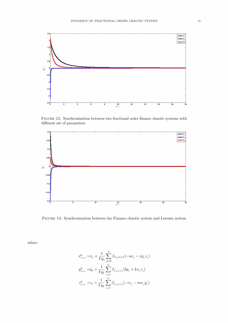
distance between two points which were at a distance of 10−7 at t = 0 and are then allowed to evolveon the attractor. Figure 11 plots the bifurcation diagram of finance chaotic system of order q = 0.98with c as the bifurcation parameter. From the figure, it is observed that there exists a critical valueof c above which the system becomes highly periodic and possibly chaotic. For values below this valueof c, the system remains stable. Similar behaviour is observed for the other two parameters a and b isincreased, it becomes chaotic after a certain value. Figure 12 shows the globally stable synchronizationof two fractional order finance chaotic system with different set of parameters for a sufficiently largevalue of the coupling factor k. The bound M needs to be guessed by letting the fractional order financesystem evolve on the chaotic attractor for a long enough period. Figure 13 shows the synchronizationbetween two structurally inequivalent fractional order systems: the finance chaotic system and Lorenzsystem. The attractor on the Lorentz system is deformed to the attractor of the finance chaotic systemin the process.


0 0.05 0.1 0.15 0.2 0.25 0.3 0.35

0.86

0.88

0.9

0.92

0.94

0.96

0.98

α →

q →

Figure 3. Two variable bifurcation diagram between α and q

0 0.05 0.1 0.15 0.2 0.25 0.3 0.351

1.5

2

2.5

3

3.5

4

4.5

α →

x 2 (m

ax)

→

Figure 4. Bifurcation diagram of controlled finance system with parameter values ofcase 2

Appendix

Appendix A. Numerical approach for solving fractional order differential equation

To solve fractional order differential equations numerically, the algorithm proposed by Diethlm [26] isconsidered here which is modified method of Adams-Bashforth-Moulton algorithm. The method is de-scribed as follows: Consider the following fractional-order differential equation:

Dqy(x) = f(t, y(t)), 0 6 t 6 T(13)

y(k)(0) = y(k)0, k = 0, 1, ........m− 1,m = [q]


0 20 40 60 80 100 120 140−2

−1

0

1

2

3

t →

x i →

0 20 40 60 80 100 120 140−3

−2

−1

0

1

2

3

t →

x i →

x1

x2

x3

x1

x2

x3

(b)

(a)

Figure 5. Behaviour of the system around E∗2 without and with feedback control

0 20 40 60 80 100 120 140−3

−2

−1

0

1

2

3

t →

x i →

0 20 40 60 80 100 120 140−2

−1

0

1

2

3

t →

x i →

x1

x2

x3

x1

x2

x3

(b)

(a)

Figure 6. Behaviour of the system around E∗3 in the absence and presence of feedback control

It is equivalent to the Volterra integral equation

(14) y(t) =

m−1∑k=0

y(k)0

tk

k!+

1

Γ(q)

∫ t

0

(t− s)q−1f(s, y(s))ds


0 0.01 0.02 0.03 0.04 0.05 0.06 0.07 0.08 0.09 0.10.82

0.821

0.822

0.823

0.824

0.825

0.826

0.827

0.828

0.829

α →

q →

Figure 7. Two variable bifurcation diagram between α and q

−2 −1.5 −1 −0.5 0 0.5 1 1.5 23

3.5

4

4.5

5

5.5

6

x1 →

x 2 →

Figure 8. The phase portrait of the fractional order(q = 0.98)finance chaotic systemfor the parameter set a = 3.6, b = 0.1, c = 1

Taking h = TN and t

n= nh, n = 0, 1, 2...., N , the system (13) can be discretized as

xn+1 =x

0+

hq1

Γ(q1 + 2)(−axp

n+1− eyp

n+1zpn+1

) +hq1

Γ(q1 + 2)

n∑j=0

α1,j,n+1(−axj− ey

jzj)

yn+1 =y

0+

hq2

Γ(q2 + 2)(byp

n+1+ kxp

n+1zpn+1

) +hq2

Γ(q2 + 2)

n∑j=0

α2,j,n+1

(byj

+ kxjzj)

zn+1 =z0 +hq3

Γ(q3 + 2)(−czp

n+1−mxp

n+1zpn+1

) +hq3

Γ(q3 + 2)

n∑j=0

α3,j,n+1

(−czj−mx

jyj)


−0.4 −0.3 −0.2 −0.1 0 0.1 0.2 0.3 0.4−0.8

−0.6

−0.4

−0.2

0

0.2

0.4

0.6

(a)−2 −1.5 −1 −0.5 0 0.5 1 1.5

−1

−0.5

0

0.5

1

(b)

−2 −1.5 −1 −0.5 0 0.5 1 1.5 2−1

−0.5

0

0.5

1

(c)−2 −1.5 −1 −0.5 0 0.5 1 1.5 2

−1

−0.5

0

0.5

1

(d)

Figure 9. Poincare sections of the Finance chaotic system

0 100 200 300 400 500 6000

0.5

1

1.5

2

2.5

3

3.5

4

t →

D →

Figure 10. Chaotic nature presented by the distance between two points of the chaotic system

0.82 0.83 0.84 0.85 0.86 0.87 0.88 0.89 0.9 0.91 0.924.5

5

5.5

6

6.5

c →

x 2 (m

ax) →

Figure 11. Bifurcation diagram of the finance chaotic system of order q = 0.98 with parameter c


0 2 4 6 8 10 12 14 16 18 20−2.5

−2

−1.5

−1

−0.5

0

0.5

1

1.5

2

2.5

t →

e i →

e1

e2

e3

Figure 12. Synchronization between two fractional order finance chaotic systems withdifferent set of parameters

0 5 10 15 20 25 30−0.2

−0.15

−0.1

−0.05

0

0.05

0.1

0.15

0.2

t →

e i →

e1

e2

e3

Figure 13. Synchronization between the Finance chaotic system and Lorentz system

where

xpn+1

=x0

+1

Γq1

n∑j=0

β1,j,n+1(−axj− ey

jzj)

ypn+1

=y0

+1

Γq2

n∑j=0

β2,j,n+1

(byj

+ kxjzj)

zpn+1

=z0 +1

Γq3

n∑j=0

β3,j,n+1

(−czj−mx

jyj)


and

αi,j,n+1 =

nqi+1 − (n− nqi )(n+ 1qi ), j=0;

(n− j + 2)qi+1

+ (n− j)qi+1 − 2(n− j + 1)qi+1, 1 ≤ j ≤ n;

1, j=n+1

βi,j,n+1 ={

hqiqi

(n− j + 2)qi + (n− j)qi , 0 ≤ j ≤ n.

The error estimate of the above scheme is maxj=0,1,.....,N

{|y(tj−y

h(tj)| = (hp), in which p = min(2, 1+q

i)

and qi> 0, i = 1, 2, 3.

References

[1] Pecora L.M.,Carrol T.L.,Synchronization in chaootic systems,Phys.Rev.Lett,64(1990), pp.821-24.[2] Park JH, Kwon OM, A novel criteria for delayed feedback control of time-delay chaotic systems, Chaos Soliton Fractal,

23(2005), pp.495-501.

[3] Chen SH, Lu J.,Synchronization of an uncertain unified chaotic system via adaptive control, Chaos Soliton Fractal,14(2002),pp. 643-647.

[4] Ho Mc, Hung YC, Synchronization of two different systems by using generalized active control, Phys Lett A,301(2002),

pp.424-429.[5] Vincent UE, Chaos synchronization using active control and back stepping control: a comparative analysis, Nonlin

Anal Model Control, 13(2008), pp.253-261.

[6] Ott E., Grebogi C.,Yorke J.A., Controlling chaos,Phys.Rev.Lett,64(1990), pp.1196-99.[7] Soczkiewicz E., Application of fractional calculus in the theory of viscoelasticity, Mol Quant Acoust,

23(2002),pp.397404.

[8] Das S., Tripathi D., Pandey SK., Peristaltic flow of viscoelastic fluid with fractional maxwell model through a channel,Appl Math Comput, 215(2010),pp.364554.

[9] Gorenflo R., Mainardi F., Fractional diffusion processes: probability distributions and continuous time random walk,In: Rangarajan G,Ding M.,editors.Processes with long range correlations,Berlin,Springer-verlag; 2003. pp. 14866 [Lec-

ture Notes in Physics, No. 621].

[10] Heaviside O., Electromagnetic theory, Chelsia, Newyork,1971.[11] Kikuchi N.,Chaos control and noise suppression in external cavity semiconductor lasers, IEEE Journal of Quantum

Electronics, 33(1997),pp.56-65.

[12] Mark J., Chaos in semuconductor lasers with optical feedback:theory and experiment, IEEE Journal of QuantumElectronics, 28(1992),pp.93-108.

[13] Magin RL., Fractional calculus in bioengineering. Part 3. Crit Rev Biomed Eng 2004;32,pp.195377.

[14] Glockle WG., Mattfeld T., Nonnenmacher TF., Weibel ER., Fractals in biology and medicine, Basel, Birkhauser; 1998.pp.2.

[15] Grigorenko I.,Grigorenko E., Chaotic dynamics of the fractional Lorenz system, Physical Review Letters,

91(2003),pp.34101-104.[16] Li C.,Peng G., Chaos in Chens system with a fractional order, Chaos Solitons and Fractals, 22(2004), pp. 443-450.

[17] Li C.,Chen G., Chaos and hyperchaos in the fractional-order Rossler equations, Physica A: Statistical Mechanics andits Applications, 341(2004), pp.55-61.

[18] Sheu L.J.,Chen H.K.,Chen J.H.,Tam L.M.,Chen W.C.,Lin K.T., Chaos in theNewton-Leipnik system with fractional

order, Chaos, Solitons and Fractals,36, (2008),pp.98-103.[19] Matouk A.E., Dynamical behaviors, linear feedback control and synchronization of the fractional order Liu system,

Journal of Nonlinear Systems and Applications, 3(2010),pp. 135140.[20] Chen L., Chai Yi., Wu R.; Control and synchronization of fractional order finance system based on linear control,

Discrete dynamics in Nature and Society, Vol-2011[21] D. Matignon. Stability result on fractional differential equations with applications to control processing.in:IMACS-SMC

Proceedings, Lille, France, July, pp.963-968, 1996.[22] D. Matignon. Stability properties for generalized fractional differential systems, in: Proc.of Fractional Differential

Systems: Models, Methods and App., vol. 5, pp.145-158, 1998.[23] D. Matignon and B. D’Andrea-Novel. Some results on controllability and observability of finite-dimensional fractional

differential systems, in: Computational Engineering in Systems Applications, vol.2, Lille, France, IMACS, IEEE-SMC,pp. 952-956, 1996.

[24] Ahmed, E. et al., On some Routh Hurwitz conditions for fractional order differential equations and their applications

in Lorenz,Rossler, Chua and Chen systems, Phys. Lett.A, 358(2006), pp. 14.

[25] Ahmed, E.,El-Sayed, A.,El-Saka, H., Equilibrium points,stability and numerical solutions of fractional order predator-prey and rabies models, Journal of Mathematical Analysis and Applications, 325(2007),pp.542-553.

[26] Diethelm K.,Ford N.J.,Freed A.D.,Luchko Yu, Algorithms for the fractional calculus: A selection of numerical meth-ods,Comput Methods Appl Mech. Engrg.194(2005)pp.743-773.

[27] Diethelm K.,Ford N.J., Analysis of fractional differential equations, Journal of Mathematical Analysis and Applica-

tions, 265(2002), 229-248.[28] Islam N.,Islam M., Islam B.; Dynamics of linear bidirectional synchronization of Shimizu Morioka system, Global

Journal of Mathematical sciences: Theory and Practical,Vol-4,No.-3(2012),pp. 279-290.


[29] Hongwu W., Junhai MA; Chaos control and synchronization of a fractional order Autonomous system,Wseas Trans-

actions on Mathematics, Vol-11,No.-8(2012).

Received: January, 2017

mathematica aeterna, vol. 7, 2017, no. 1, 1 - 17 · 1department of applied science, rcciit,...

Documents