mathematica - media.wolfram.commedia.wolfram.com/documents/scientificastronomerdocumentation.pdf ·...
TRANSCRIPT


Mathematica® is a registered trademark of Wolfram Research, Inc.
All other product names mentioned are trademarks of their producers. Mathematica is not associated with Mathematica Policy Research, Inc. or MathTech, Inc.
March 1997First edition, Intended for use with either Mathematica Version 3 or 4
Software and manual written by: Terry Robb Editor: Jan Progen Proofreader: Laurie Kaufmann Graphic design: Kimberly Michael
Software Copyright 1997–1999 by Stellar Software. Published by Wolfram Research, Inc., Champaign, Illinois.
All rights reserved. No part of this document may be reproduced, stored in a retrieval system, or transmitted in any form or by any means, electronic, mechani -cal, photocopying, recording or otherwise, without the prior written permission of the author Terry Robb and Wolfram Research, Inc.
Stellar Software is the holder of the copyright to the Scientific Astronomer package software and documentation (“Product”) described in this document, includingwithout limitation such aspects of the Product as its code, structure, sequence, organization, “look and feel”, programming language and compilation ofcommand names. Use of the Product, unless pursuant to the terms of a license granted by Wolfram Research, Inc. or as otherwise authorized by law, is aninfringement of the copyright.
The author Terry Robb, Stellar Software, and Wolfram Research, Inc. make no representations, express or implied, with respect to this Product, includingwithout limitations, any implied warranties of merchantability or fitness for a particular purpose, all of which are expressly disclaimed. Users should beaware that included in the terms and conditions under which Wolfram Research, Inc. is willing to license the Product is a provision that the author TerryRobb, Stellar Software, Wolfram Research, Inc., and distribution licensees, distributors and dealers shall in no event by liable for any indirect, incidental orconsequential damages, and that liability for direct damages shall be limited to the amount of the purchase price paid for the Product.
In addition to the foregoing, users should recognize that all complex software systems and their documentation contain errors and omissions. The authorTerry Robb, Stellar Software, and Wolfram Research, Inc. shall not be responsible under any circumstances for providing information on or corrections toerrors and omissions discovered at any time in this document or the package software it describes, whether or not they are aware of the errors or omissions.The author Terry Robb, Stellar Software, and Wolfram Research, Inc. do not recommend the use of the software described in this document for applicationsin which errors or omissions could threaten life, injury, or significant loss.
10 9 8 7 6 5 4 3
#T2261 12/8/2000

Table of Contents
Graphics Gallery v
1. Introduction 1About the Package • Loading and Setup • Installation and Notebooks • Palettes and Buttons
2. Basic Functions 13The Ephemeris and Appearance Functions • The PlanetChart and EclipticChart Functions •The Planisphere Function • The SunRise and NewMoon Functions • The BestView and InterestingObjects Functions
3. Coordinate Functions 35The EquatorCoordinates Function • The HorizonCoordinates Function • The Coordinates Function • The JupiterCoordinates Function
4. Star Charting Functions 47The StarChart Function • The RadialStarChart Function • The CompassStarChart Function • The ZenithStarChart Function • The StarNames Function • The OrbitTrack and OrbitMark Functions • The ChartCoordinates and ChartPosition Functions
5. Planet Plotting Functions 85The PlanetPlot Function • The PlanetPlot3D Function • The RiseSetChart Function • The VenusChart Function • The OuterPlanetChart Function • The PtolemyChart Function • The SolarSystemPlot Function • The JupiterSystemPlot Function • The JupiterMoonChart Function
6. Eclipse Predicting Functions 119The EclipseTrackPlot Function • The MoonShadow and SolarEclipse Functions • The EclipseBegin and EclipseEnd Functions • The EclipseQ Function • The Conjunction and ConjunctionEvents Functions
7. Satellite Tracking Functions 137The SetOrbitalElements Function • The GetLocation Function • The OrbitTrackPlot Function • The OrbitPlot and OrbitPlot3D Functions
8. Miscellaneous Functions 153The Separation and PositionAngle Functions • The FindNearestObject Function • The SiderealTime and HourAngle Functions • The Lunation and LunationNumber Functions • The NGC and IC Functions
9. Additional Information 167Ephemeris Accuracy • Using PlanetChart • Using StarChart • Using RadialStarChart • Planetographic Coordinates

Appendix. Special Events 175Meteor Showers • Sunspots • Solar Eclipses • Lunar Eclipses • Transits of Mercury • Transits of Venus • Saturn’s Rings Edge On • Uranus’ Poles Side On • Mercury Apparitions • Venus Apparitions • Mars Opposition • Jupiter Opposition • Saturn Opposition • Lunar Occultations • Eclipse Table • Deep Sky Data • Brightest Stars • Double Stars • Variable Stars • Planetary Data • Visible Earth Satellites • Deep Sky Objects
Index 199

Graphics Gallery v
Main Features of Scientific AstronomerStar Charts: Five types of charts are defined in Scientific Astronomer,including two wide field star charts. With the star charts you can zoom intoany portion of the sky. All the charts have options to show star spectral colors,mesh lines, a skyline, the horizon line, and the Milky Way; and to labelconstellations, stars, planets, deep sky objects, and so on.
Planet Plots: Planet plotting is done in two- and three-dimensional forms.Surface features for the Earth, the Moon, Mars, and Jupiter are shown on theplots. Moons and their shadows are displayed for the Earth and Jupiter.Related functions allow you to produce planet position finder charts and planetrise/set timing charts.
Eclipses: Several functions are provided for dealing with eclipses. Thesefunctions provide information about both solar and lunar eclipses, and aregeneral enough to handle Galilean moon eclipses, occultation of stars by theMoon, and transits of Mercury or Venus across the solar disk. You canproduce umbra and penumbra track plots and perform eclipse prediction.
Satellite Tracking: Satellite tracking is another feature of ScientificAstronomer. You can create track plots, make visibility predictions, andproject satellite tracks onto star charts.
Miscellaneous: Miscellaneous other features are available, such as producingplanisphere plates, planet charts, and solar system plots. In addition, sunrise,moonrise, and full moon functions are provided, as well as functions foradding new objects, such as comets and satellites.
Scientific Astronomer is Mathematica 3 and 4 compatible. It has palettes andbuttons and is fully integrated into the Help Browser system.
Terry Robb, March 1997.
Feature Labeling on the Moon
MareCrisium
MareFoecunditatis
MareNectaris
MareTranquillitatis
MareSerenitatis
MareVaporum
Mare Frigoris
MareNubium
MareImbrium
MareHumorum
OceanusProcellarum
Plot of a full moon with features labeled.
Mercury Finder Chart
Morning Evening
Mercury
2am 4am 6am 8am 10am 1994 2pm 4pm 6pm 8pm 10pm
Jan
Feb
Mar
Apr
May
Jun
Jul
Aug
Sep
Oct
Nov
Dec
Autumn
Winter
Spring
Summer
Chart showing rising and setting times of Mercury during 1994 for an observer 35 degreessouth of the equator. Green areas (or the darker shade of gray) show when Mercury isvisible above the horizon.
Morning
Morning
Evening
Evening
HaleBopp
2am 4am 6am 8am 10am 1997 2pm 4pm 6pm 8pm 10pm
Jan
Feb
Mar
Apr
May
Jun
Jul
Aug
Sep
Oct
Nov
Dec
Spring
Summer
Autumn
Winter
Chart showing rising and setting times of Comet Hale-Bopp during 1997 for an observer40 degrees north of the equator. Green areas show when Hale-Bopp is visible.
Star Chart of Ophiuchus
19h 18h 17h 16h-45
-30
-15
0
15
30
45Sector5
Aquila
CoronaAustralis
Hercules
Lyra
Ophiuchus
Sagitta
Sagittarius
Scorpius
Scutum
Serpens
Star chart showing various constellations in the direction of Ophiuchus. Scorpius isvisible on the bottom right. The blue line near the bottom is the ecliptic, which is the fixedpath of the Sun through the sky. The planets and Moon all roughly move along that line aswell.

Milky Way and Nebulae
19h 18h 17h 16h
�45
�40
�35
�30
�25
�20
�15
�10
�5
0
5
Antares
CoronaAustralis
Ophiuchus
Sagittarius
Scorpius
Scutum
Serpens
NGC:6611
NGC:6618
NGC:6514NGC:6523
Star chart showing the Milky Way in the region of Scorpius and Sagittarius. Fourbinocular-visible nebulae are indicated by the position of the yellow NGC numbers. Starspectral colors of stars, such as red for Antares, are also indicated.
Jupiter's Moons and Great Red Spot
K=12 Impact
{1994, 7, 19, 20, 15, 0}
Fragment of Comet P/Shoemaker-Levy impacting on Jupiter. Two Jovian moons and theGreat Red Spot are visible. This graphic is part of a large animation.
Retrograde Motion of Mars
8h 6h 4h-20
-15
-10
-5
0
5
10
15
20
25
30
35
40
Cancer
CanisMinor
Gemini
Monoceros
Orion
Taurus
Star chart track of Mars undergoing retrograde motion during 1992.
Eight-Year Venus Finder Chart
1994
1995
19961997
1998
1999
2000
2001
JFMA
M
J
J
A
S
O
ND
J
F
M
A
M
J
J
ASO
N
D
J
F
M
A
M
J J
A
S
O
N
D
J
F
MAMJ
J
A
S
O
N
D
JF
M
A
M
J
J
A
S
OND
JFM
A
M
J
J
A
S
O
N
D
J
F
M
A
MJ
JAS
O
N
D
J
F
M
AM
J
J
A
S
O
N
D
Earth
Sun
Venus
Morning
Morning
Evening
Evening
Finder chart for Venus for years 1994 through 2001.
vi Graphics Gallery

Plot of Earth
Plot of Earth as viewed from directly over Melbourne, Australia. The darker arearepresents night, which is the half of the globe not illuminated by the Sun.
Optional Labeling
6h 5h
�15
�10
�5
0
5
10
15
20
Rigel
Betelgeuse
Aldebaran
β
α γ
εζ
κ
δ
ι
π3
η
Star chart of constellation Orion using double-size labeling.
Lunar Eclipse Chart
Moon
Partial
22:10
Begin
Total
23:11
Begin
Total
00:46
End
Partial
01:47
End
WestEast
Penumbra
Umbra
1993�Jun�04 23:58:33
Partial for 217 min. Total for 96 min.
Chart showing circumstances of a total lunar eclipse.
Overhead Sky
NorthNorth
South
East West
Nov 17
03:20
Latitude
38 South
Star chart showing entire overhead sky as seen from latitude 38 degree south at 03:20 onNovember 17. The Milky Way is the dark blue band across the sky.
Graphics Gallery vii

Solar Eclipse Chart
Chart showing circumstances of the total solar eclipse of 1948 November 1. The blackline is the line of totality and the gray region is where a partial eclipse was visible.
Plot of the eclipse as it moves off the eastern edge of Africa. The shaded region on the leftside of the Earth is night.
Compass Direction Star Chart
East South West
Jan 01
01:00
Latitude
38 South
Star chart showing the southern aspect of the sky. Our Milky Way galaxy is the verticalblue band slightly to the left. The chart below shows the northern aspect.
West North East
Jan 01
01:00
Latitude
38 South
Solar Eclipse of 1998
Chart showing circumstances of the total solar eclipse of 1998 February 26. The blackline is the line of totality, which passes directly through Panama but otherwise is visibleonly over the ocean. The gray region is where a partial solar eclipse is visible.
Chart showing eclipse shadow at a particular instant. The dark region covering most ofthe right of the graphic represents the night side of the Earth. The small black dot at thetop of South America is the point of total eclipse at the given instant.
Motion of Asteroid Vesta
15h40m 15h20m 15h00m 14h40m 14h20m 14h00m-30
-25
-20
-15
-10
-5
0
Libra
1
23
4
56
7
8
Plot showing orbital track of asteroid Vesta during opposition in 1996. Blue numbers aremonths of that year; Vesta reaches its brightest at month 5 (May).
viii Graphics Gallery

Comet Hale-Bopp Location
Andromeda
Aries
Camelopardalis
Cassiopeia
Cepheus
Lacerta
Pegasus
Perseus
Pisces
Triangulum
0.5 Hour 36. Degree
RadialAngle: 50. Degree
3
3
6
6
9
9
12
12
15
15
18
18
21
21
24
24
27
27
30
30
2
2
5
5
8
8
11
11
14
14
17
17
20
20
Star chart track of Comet Hale-Bopp (shown in red) during closest approach in March/April 1997. The track of the Sun (in orange) is also shown. Blue lines represent thedirection of the comet tail.
Big Dipper with Greek Labels
CanesVenatici
UrsaMajor
UrsaMinor
12. Hour 59. Degree
RadialAngle: 20. Degree
ε
α
η
ζ β
γ
ψ
δ
Star chart of Ursa Major, also known as “The Big Dipper” or “The Plough”.
Mercator Projection of Sky
22h 20h 18h 16h 14h 12h 10h 8h 6h 4h 2h 0h-90
-60
-30
0
30
60
90
Star chart showing entire celestial sphere in Mercator projection. The light blue shadedarea is our own Milky Way galaxy with the galactic plane shown in red.
22h 20h 18h 16h 14h 12h 10h 8h 6h 4h 2h 0h
�60
�30
0
30
60
90
Star chart showing positions of many galaxies. Most galaxies lie in a plane (the plane ofthe local supercluster of galaxies). Note the Virgo Galaxy Cluster near the center of thegraphic. The circles on the lower right are the Large and Small Magellanic CloudGalaxies. The small circle to the top right is the Andromeda Galaxy.
Annual Meteor Showers
0 90. Degree
RadialAngle: 120. Degree
10amJan03
5amApr22
9amMay03
3amJul29
1amJul30
7amAug12
6pmOct10
6amOct22
2amNov03
8amNov18
3amDec14
10amDec23
Chart showing main annual meteor showers visible from the Northern Hemisphere. Theyellow disks indicate viewing direction, with date and best viewing hour given inside.
Graphics Gallery ix

Astrological Aspect Chart
Astrological aspect chart for the main planets on a given date and location. The symbolson the diagonal are, from top-left to bottom-right: the ascendant, the Sun, the Moon,Mercury, Venus, Mars, Jupiter, and Saturn.
Solar System Plot
0h
Psc
2h
Ari
4h
Tau6h
Gem
8h
Cnc
10h
Leo
12h
Vir
14h
Lib
16h
Sco18h
Sgr
20h
Cap
22h
Aqr
Morning
Evening
1993-Nov-17
Solar system plot showing positions of planets out to Saturn. The Earth is in the centerwith the Sun shown in yellow and Mercury very close to it.
Orbit Plot of Outer Planets
Plot showing orbits of the outer planets. Pluto's orbit is the outermost inclined ellipse,which can pass inside Neptune's orbit.
Mars as Seen from Earth
Plot of Mars as seen from Earth on a given date. The green cross on the far right is theposition of zero Martian longitude and latitude.
x Graphics Gallery

Mir Space Station Flyover
Sirius
Canopus
RigilKent
Capella
Rigel
Procyon
Achernar
Betelgeuse
Acrux
Aldebaran
Pollux
Fomalhaut
Regulus
Adhara
Castor
Pleiades
NorthNorth
South
East West
Feb 01
21:50
Latitude
38 South
Track of Mir Space Station flying overhead. It takes about 10 minutes for Mir to passfrom the southwest horizon over the zenith and down into the northeast horizon.
Deep Sky Objects
8h 6h 4h
�30
�15
0
15
30
Flaming Star Nebula
California
M42 Nebula
M35 Cluster
Rosette Nebula
Crab NebulaEskimo Nebula
Christmas Tree
2362
M47
M41
Orion
Taurus
Sirius
Rigel
ProcyonBetelgeuse
Aldebaran
Pollux
Castor
Finder chart for various interesting deep sky objects (such as nebulae, star clusters, andgalaxies) in the direction of Orion.
Astrological Birth Chart
Birth chart for Charles Dickens, born at midnight on 1812 February 7 in England.
Space Shuttle Orbit
Four orbits of a Space Shuttle mission. The light red areas indicate the locations on Earth,where the Space Shuttle will be visible to the naked eye just after dusk as it movesoverhead. Similarly, the light blue area indicates visibility just before dawn.
Chart zoomed into area around Australia showing the track of the Space Shuttle. Theshading on the right is the approaching night.
Graphics Gallery xi

Comet Hale-Bopp 1996-1998
22h 20h 18h 16h 14h 12h 10h 8h 6h 4h 2h 0h-90
-60
-30
0
30
60
90
6 7 8 9
101112
13
14
1516
17
18
19
20
21
22
23
24 2526
14
15
16
171819
20
Star chart showing position of Comet Hale-Bopp from April 1996 through April 1998.The blue numbers represent months from the beginning of 1996. Orange numbers are thecorresponding positions of the Sun.
16 Mar 1997
16 Mar 1997
Part of a stereographic animation showing the motion of the Comet Hale-Bopp and Earthrelative to the Sun at the center.
Motion of Mir Space Station
Sirius
Capella
Rigel
ProcyonBetelgeuse
Aldebaran
Pollux
Regulus
Adhara
Castor
Pleiades
X
50
51
52
53
5455
West North East
Feb 01
21:50
Latitude
38 South
Star chart showing track of Mir Space Station setting into the northeast horizon. Rednumbers represent minutes, and the blue X is where Mir will disappear when it movesinto the Earth's shadow.
Orbit track showing the motion of Mir as it passes over Melbourne, Australia.
Planet Wall Chart1994 Planet Chart
New
Moon Sun Mercury Venus Mars Jupiter Saturn
Full
Moon
Meteor
Shower
Transit
Time 3am: 1am:
11pm: 9pm:
MarAprMayJun
FebMarAprMay
JanFebMarApr
DecJanFebMar
NovDecJanFeb
OctNovDecJan
SepOctNovDec
AugSepOctNov
JulAugSepOct
JunJulAugSep
MayJunJulAug
Evening
Morning
Evening
Morning
2
4
6
8
10
12
10
8
6
4
2
2
4
6
8
10
12
10
8
6
4
2
Setting
Hours after Sunset
0
2
4
6
8
Rising
Hours before Sunrise
2
4
6
8
Jan
Feb
Mar
Apr
May
Jun
Jul
Aug
Sep
Oct
Nov
Dec
Sirius
Arcturus
Procyon Orion AltairAldebaran
Antares
Spica
Pollux
Fomalhaut
Regulus
PleiadesNorth North
South South
Ecliptic
Right Ascension<- East Horizon West Horizon ->
N
S
+23
-23
18h
Sco
16h
Lib
14h
Vir
12h
Leo
10h
Cnc
8h
Gem
6h
Tau
4h
Ari
2h
Psc
0h
Aqr
22h
Cap
20h
Sgr
18h
Wall chart showing positions of major planets throughout 1994.
Stereographic Pairs
Stereographic pair showing orbital planes of the GPS (Global Positioning System)satellite network. Converge your eyes to view in full 3D. The red, green, and blue orbitsare mutually orthogonal to each other, as are the cyan, magenta, and yellow orbits.
Stereographic pair showing the local supercluster of galaxies. Our Local Group ofgalaxies is the small blue object in the center of the graphic. Just next to it is the VirgoGalaxy Cluster shown in green. Beyond that is the Coma Galaxy Cluster in red, and thePisces Galaxy Cluster in yellow. The large Centaurus Galaxy Cluster is shown in purple.The box is one billion light years across.
xii Graphics Gallery

1. IntroductionScientific Astronomer is a Mathematica package implementing graphical and other tools of interest toamateur and professional astronomers.
The package produces charts, generates animations, and derives information to help you learn moreabout astronomical events. For instance, if you hear about a new event, such as a bright comet, aneclipse, or a lunar occultation, Scientific Astronomer allows you to determine the location and details ofthe event. Similarly, you can use the package to re-create the circumstances of ancient eclipses, planetaryalignments, and other events of historical significance. A very simple application is to discover, forexample, the phase of the Moon on the day you were born.
Scientific Astronomer generates finder charts for interesting objects in the sky. The night sky is full offamiliar and unusual objects, many of which are visible to the naked eye. Most of us have seen theplanet Venus and could identify a few constellations, but there are many other astronomical objects andevents visible to the naked eye. A few possibilities include a meteor shower, the Mir Space Station, alunar eclipse, the planet Mercury, the asteroid Vesta, a colorful star, a double star, a variable star, a starcluster, or a galaxy. All these objects are visible on clear dark nights at an appropriate time of the year.
The trick to sighting such objects is to know where and when to look. Scientific Astronomer gives you thetools to determine “the where” and “the when”.
Aided with good binoculars, you can see even more objects, such as Jupiter’s moons, Saturn’s rings,various comets, diffuse nebulae, and a few galaxies. Again, Scientific Astronomer gives you the tools tolocate the objects and to reproduce and predict the circumstances of their appearance.
About the Package
Scientific Astronomer includes over 9,000 stars, and it can determine the positions of all the planets, theSun, the Moon, and other objects on any given date for thousands of years into the past or future. It alsoincludes a large number of deep sky objects.
Scientific Astronomer covers four main areas of astronomy. It has functions for star charting, planetplotting, eclipse predicting, and satellite tracking. There are, of course, a large number of other functionsand features in the package.
Five types of charts are defined in Scientific Astronomer, including two wide field star charts. With thestar charts you can zoom into any portion of the sky. All the star charts have options to show spectralcolors, mesh lines, a sky line, the horizon line, and the Milky Way; and to label constellations, stars,planets, deep sky objects, and so on.
Planet plotting is done in either two- or three-dimensional forms. Surface features for the Earth, theMoon, Mars, and Jupiter are shown on the plots. Moons, and their shadows, are displayed for the Earthand Jupiter. Related functions allow you to produce planet position finder charts and planet rise/settiming charts.
About the Package 1

The package provides several functions for dealing with eclipses. These functions provide informationabout both solar and lunar eclipses, and are general enough to handle Galilean moon eclipses,occultation of stars by the Moon, and transits of Mercury or Venus across the solar disk. You canproduce umbra and penumbra track plots and perform eclipse prediction.
The satellite tracking feature of Scientific Astronomer allows you to create track plots, make visibilitypredictions, and project satellite tracks onto star charts.
Miscellaneous features are available, such as producing planisphere plates, planet charts, and solarsystem plots. In addition, sunrise, moonrise, and full moon functions are provided, as well as functionsfor adding new objects such as comets and satellites.
Overall, Scientific Astronomer provides a large number of tools of interest to professional and amateurastronomers. Not only does the package contain standard planetarium-type features for generating starcharts, but it has functions that when used in conjunction with Mathematica create a general astronomycomputing environment.
Scientific Astronomer is fully compatible with Mathematica Versions 3 and 4. The package has many palettesand hyperlinks, and is fully documented in the Help Browser.
2 1. Introduction

� 1.1 Loading and Setup
Once you have installed the package, it is a simple matter to load it into Mathematica.
�� Astronomer `HomeSite ` load the package and set details for your home site
Loading the package.
� This loads the package into Mathematica.
In[1]:= <<Astronomer`HomeSite`
Astronomer is Copyright (c) 1997 Stellar Software
Depending on your computer, it may take a minute or so to load if you are using Mathematica Version 2.Scientific Astronomer will take less than ten seconds to load using Mathematica Version 3, however.
Site Location
If you have not already edited the HomeSite.m file with your site details, then you need to useSetLocation to define your geographic longitude, latitude, and time zone.
SetLocation�options� set the location and time zone on the surface of the Earth
GeoLongitude �� longitude the geographic longitude, where east is positive
GeoLatitude �� latitude the geographic latitude
GeoAltitude �� altitude the geographic altitude in kilometers
TimeZone :� timezone the time zone, or hours ahead of GMT �Greenwich Mean Time�
Setting your site location.
� This is the setup for Melbourne, Australia during daylight-saving time.
In[2]:= SetLocation[GeoLongitude -> 145.0*Degree, GeoLatitude -> -37.8*Degree, GeoAltitude -> 0.0*KiloMeter, TimeZone -> 11];
You can put any SetLocation setting into your HomeSite.m file to avoid having to enter it everysession. Typically you can use the option setting TimeZone :> TimeZone[] to dynamically computeyour time zone. Throughout this user’s guide, the TimeZone option is set to 11, which is appropriate forsummertime in Melbourne, Australia. It is very important that you use the correct time zone for yourown location, as some functions will give inappropriate results otherwise. In particular, be careful thatdaylight-saving time is taken into account. When daylight saving is in effect over summer, the value
1.1 Loading and Setup 3

returned by TimeZone[] should be one hour greater than normal. Thus, the normal time zone valuesfor the Pacific, Central, and Eastern zones of the United States are -8, -6, and -5, respectively; but for aperiod within April through October, the values are -7, -5, and -4, respectively.
Note that the sign of the option GeoLongitude is such that positive is east and negative is west. Thus,the geographic longitude of Champaign, Illinois is -88.2 degrees, a negative number because it is west ofGreenwich.
You can rename the HomeSite.m file, if you wish. For example, you might want to call it NewYork.m,and configure it for the geographic location of New York. In that case, you can start Scientific Astronomerby typing <<Astronomer`NewYork` . Similarly, you can create other site files, such as London.m orTokyo.m.
Degree Character
The degree symbol, which is used in the output from Ephemeris and other functions, might not printor display correctly if you are running Scientific Astronomer under a version of Mathematica earlier than3.0. Some computer systems do not have an appropriate character available, and in such cases you needto set the variable $DegreeCharacter to something tolerable to your system.
Although Scientific Astronomer tries to figure out the correct character, it may become confused if you arerunning a remote kernel. If your front end is a Unix machine running X Windows or a PC runningWindows, you may need to use character 176, that is, $DegreeCharacter =FromCharacterCode[176]. If your front end is a Macintosh, you may need to use character 161, thatis, $DegreeCharacter = FromCharacterCode[161] . If all else fails, you can set the variable to thecharacter “^”, that is, $DegreeCharacter = "^".
Under Mathematica Version 3.0 or later, $DegreeCharacter is always correctly set for you.
Font Names and Sizes
Labeling of star charts and other graphical output is mostly done with the default font “Helvetica”. Ifyou are not satisfied with that font, change it by setting the variable $DefaultFontName to anotherfont name, such as “Arial”, “Times-Italic”, or “Courier”, for instance.
$DefaultFontScale increase the size of fonts in graphics; default is 1
$PointSizeScale increase the size of points in graphics; default is 1
$ThicknessScale increase the size of lines in graphics; default is 1
Adjusting sizes of fonts, points, and lines.
Similarly, if you prefer another size of labeling on your monitor or printer, you can set the variable$DefaultFontScale to a scale factor other than the default 1. To increase point sizes and linethicknesses, use the variables $PointSizeScale and $ThicknessScale. On a PC running Windowsyou will typically need to set $PointSizeScale = 2, but your screen resolution will determinewhether this is actually an improvement.
4 1. Introduction

These changes can be made globally and put in the HomeSite.m file if needed.
Note that although you can use $DefaultFontScale to adjust some font sizes used in the package,you will normally use the TextStyle option for this.
Extra Stars
By default, a small number of stars are built directly into the package. These stars are enough to allowall the Scientific Astronomer features to work. You need to load more stars if you require more detailedstar charts.
�� Astronomer `Star3000 ` load the 3,000 naked-eye visible stars
�� Astronomer `Star9000 ` load the 9,000 binocular visible stars
�� Astronomer `DeepSky ` load various nebulae, star clusters, and galaxies
Loading extra stars and objects.
� This loads 3,000 extra stars. Similarly, you can load a file containing 9,000 extra stars.
In[3]:= <<Astronomer`Star3000`
One disadvantage to loading extra stars is that it potentially causes some of the star chart functions toslow down, especially on the first call.
The default setup, therefore, includes only the brightest 300 stars, which are more than enough to allowbasic constellation identification. The default setup includes all the stars down to magnitude 3.5 andseveral additional ones.
Once Star3000.m has been loaded, all the 3,000 naked-eye visible stars down to magnitude 5.5 areused. Similarly, with Star9000.m loaded, all the 9,000 binocular visible stars down to magnitude 7.5are used.
Stars represent only a part of what is in the universe; many nonstellar objects, such as galaxies, nebulae,and clusters are also present. Some well-known objects, such as the Andromeda Galaxy and the Pleiadesstar cluster, are already built into Scientific Astronomer, and it is possible to access many more by loadingthe DeepSky.m package.
� This loads extra deep sky objects.
In[4]:= <<Astronomer`DeepSky`
See the corresponding DeepSky.nb notebook for a discussion on how to access and work with deepsky objects.
1.1 Loading and Setup 5

� 1.2 Installation and Notebooks
Scientific Astronomer is distributed CD-ROM. The CD-ROM contains one folder called Astronomer.
To install the package you should use the installer program on the CD-ROM. Another way to install is tomove the Astronomer folder inside Mathematica’s AddOns/Applications/ directory. Optionally,you can move the Astronomer folder to the top level of your own home directory.
README installation instructions
HomeSite.m local site details
Astronomer .m the package itself
Star3000.m an optional load file
Star9000.m an optional load file
DeepSky .m an optional load file
Documentation � user’s guide
FrontEnd � front end files
Kernel � kernel files
Files needed by the package.
Refer to the README file for additional instructions on how to install the package, and on how tocustomize it for your purposes. The most important task is to edit the HomeSite.m file with your ownsite details. In that file you will see site details commented out for many cities. If you live in one of thesecities, simply uncomment the setting.
The CD-ROM also includes an on-line version of this user’s guide. Once you have installed ScientificAstronomer, you will need to open the Help menu in the Mathematica front end and choose RebuildHelp Index. This will make the user’s guide, and other information, available in the front end HelpBrowser.
6 1. Introduction

Cover .nb cover page
Contents .nb table of contents
Chapter1 .nb introduction
Chapter2 .nb basic functions
Chapter3 .nb coordinate functions
Chapter4 .nb star charting
Chapter5 .nb planet plotting
Chapter6 .nb eclipse predicting
Chapter7 .nb satellite tracking
Chapter8 .nb miscellaneous
Chapter9 .nb additional information
Appendix .nb appendix
Index .nb index
Notebooks � sample notebooks
Palettes � palettes
On-line version of the user’s guide.
Worked Examples
Many worked examples are given in the sample notebooks that come with Scientific Astronomer. Thesesample notebooks are contained in the Astronomer/Documentation/English/Notebooks/directory. You can open the notebooks directly, or you can access them from within the Help Browser.
1.2 Installation and Notebooks 7

Apollo .nb Apollo lunar landings
Asteroids .nb asteroid trajectories
Astrology .nb astrological readings
Charts .nb star chart examples
Comets .nb comets Halley and Hale-Bopp
DeepSky .nb atlas of galaxies and nebulae
Eclipses .nb solar and lunar eclipses
Features .nb main features of package
Gallery .nb some graphic examples
Impact .nb Jupiter-comet impact
Lunar .nb lunar libration
Meteors .nb meteor showers
Mir .nb visible satellites
PlanetAnimations .nb planet animations
Satellites .nb Earth satellites
Scale .nb large-scale structure
StarMaps .nb making sky maps
Variables .nb variable stars
Viking .nb Viking Mars landings
Voyager2 .nb Voyager II trajectory
Window .nb star view from a window
585 BC .nb famous eclipse of 585 B . C .
Sample notebooks included with Scientific Astronomer .
The sample notebooks cover topics such as satellite tracking, annual meteor showers, eclipses, variablestars, comets, asteroids, and deep sky objects.
Each notebook deals with a particular aspect of astronomy and uses Scientific Astronomer to produceuseful information. For instance, the deep sky notebook contains an atlas of galaxies, nebulae, and starclusters and it uses Scientific Astronomer to create finder charts for various interesting objects, sorted bylocation and date of visibility. The comets notebook shows how to make finder charts for comets such asHalley or Hale-Bopp. Similarly, the satellite tracking notebook shows how to track the Mir Space Stationor a Space Shuttle mission. This notebook also includes an analysis of the 24 Global Positioning System(GPS) satellites. The variable stars notebook has Mathematica expressions for predicting the time ofmaximum brightness of eclipsing binaries and pulsating stars.
Studying the sample notebooks should give you a feel for the types of applications and calculations thatScientific Astronomer can handle.
8 1. Introduction

� 1.3 Palettes and Buttons
Scientific Astronomer takes full advantage of palettes in Mathematica Versions 3 and 4.
To make a palette of common functions visible from within the front end via the File � Palettes menuwhen running Mathematica Version 3, you should copy the palette notebook Astronomer/FrontEnd/Palettes/Astronomer.nb to $TopDirectory/Configuration/FrontEnd/Palettes/Astronomer.nb.This palette is also available in the Help Browser. Once you have placed the notebook in this directory,an Astronomer palette will be available. You can access it like any of the standard palettes that comewith Mathematica.
To bring up the Astronomer palette, open the File menu, move to Palettes, then choose Astronomer.
1.3 Palettes and Buttons 9

The main Astronomer palette contains a simplified function-usage listing. When you click a triangle onthe left of the palette, a list of functions in the selected category is opened.
A short note is printed at the bottom of the palette to describe the purpose of the function that themouse pointer is currently over. Click the options field to bring up a palette of options for the function.On-line help can be obtained by clicking the blue question mark on the right-hand side of each function.
If you type the name of an object in your current notebook, highlight it with the mouse, and then click afunction in the Astronomer palette, the function wraps around the object. To save typing an object youcan choose it from the basic objects palette. Alternatively, you can click the function, then choose anobject.
10 1. Introduction

The main Astronomer palette has buttons to launch additional palettes of astronomical objects.
Another feature of the main Astronomer palette allows you to launch an interactive star chart explorer.
1.3 Palettes and Buttons 11

2. Basic FunctionsMore than 70 functions are implemented in Scientific Astronomer. There are 24 graphical functions usedto produce finder charts, planet plots, and star charts. Most of the other functions simply returnnumbers or rules relating to the conditions of planets, stars, and other objects.
Apart from star charts, which constitute a large portion of Scientific Astronomer, there are a number ofbasic functions that you may find useful, especially when first learning to use the package. This chapterdiscusses the general usage of those functions.
Before you can use the package, however, you need to understand a few basic concepts and conventions.Most functions require an object and/or a date as part of the argument list, and other arguments andoptions may also be needed in some cases. Once you become familiar with the objects and date format,then using each of the functions should be relatively straightforward.
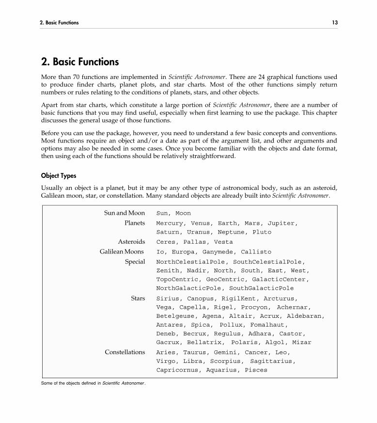
Object Types
Usually an object is a planet, but it may be any other type of astronomical body, such as an asteroid,Galilean moon, star, or constellation. Many standard objects are already built into Scientific Astronomer.
Sun and Moon Sun, Moon
Planets Mercury, Venus, Earth, Mars, Jupiter,
Saturn, Uranus, Neptune, Pluto
Asteroids Ceres, Pallas, Vesta
Galilean Moons Io, Europa, Ganymede, Callisto
Special NorthCelestialPole, SouthCelestialPole,
Zenith, Nadir, North, South, East, West,
TopoCentric, GeoCentric, GalacticCenter,
NorthGalacticPole, SouthGalacticPole
Stars Sirius, Canopus, RigilKent, Arcturus,
Vega, Capella, Rigel, Procyon, Achernar,
Betelgeuse, Agena, Altair, Acrux, Aldebaran,
Antares, Spica, Pollux, Fomalhaut,
Deneb, Becrux, Regulus, Adhara, Castor,
Gacrux, Bellatrix, Polaris, Algol, Mizar
Constellations Aries, Taurus, Gemini, Cancer, Leo,
Virgo, Libra, Scorpius, Sagittarius,
Capricornus, Aquarius, Pisces
Some of the objects defined in Scientific Astronomer .
2. Basic Functions 13

In general, an object represents some real or abstract point in the universe. You can add new objectssuch as satellites or comets whenever you wish. Many deep sky objects, such as galaxies, nebulae, andstar clusters, can be loaded using the DeepSky.m package, which includes all nonstellar objects with amagnitude at least as low as 11.
Deep Sky Clusters Hyades, Pleiades, ThetaCarinaeCluster,
BeehiveCluster, JewelBoxCluster, etc .
Deep Sky Nebulae CoalSackNebula, TarantulaNebula, OrionNebula,
LagoonNebula, RosetteNebula, etc .
Deep Sky Galaxies LargeMagellanicCloud, SmallMagellanicCloud,
AndromedaGalaxy, TriangulumGalaxy, etc .
Some deep sky objects.
There are 110 deep sky objects built directly into Scientific Astronomer. Built-in deep sky objects are givenspecial names, such as BeehiveCluster, OrionNebula, and AndromedaGalaxy; and they includeall the most notable clusters, nebulae, and galaxies that an amateur is likely to see.
About a quarter of the built-in deep sky objects are visible to the naked eye, and another half onlyrequire binoculars. The remainder require a telescope.
Other built-in objects include the nine planets, some asteroids, many named stars, and all theconstellations.
Date Formats
There are several conventions for writing calendar dates, with the two most widely used being theAmerican and European formats. A less common convention, known as scientific format, is used byastronomers. Scientific format has been adopted for dates in this user’s guide.
In scientific format, the year is written first, followed by the month, and then the day. For example, the17th day of November in the year 1993 A.D. is written in scientific format as “1993 November 17”. InAmerican format that date would appear as “November 17, 1993”; and in European format, as “17November 1993”.
You may input dates into Scientific Astronomer in several formats. For example, you can use{1993,11,17,3,20,0} to specify the local time of 3:20am on 1993 November 17. This format ismodeled exactly on the output of Date.
Another format is to use {1993,11,17}, which specifies local midnight. An alternative is to use{1993,1,321}, which means the 321st day of January, and is equivalent to {1993,11,17,0,0,0} . Itis also possible to use {1993,11,17.75}, which represents 18:00 hours (or 6:00pm) local time onNovember 17.
14 2. Basic Functions

All dates returned by Scientific Astronomer are in local time; that is, your time zone is always taken intoaccount. To get Universal Time (UT) or Greenwich Mean Time (GMT), subtract your time zone valuefrom any local date. For instance, in the examples used throughout this user’s guide, where TimeZone-> 11, the local date {1993,11,17,3,20,0} corresponds to {1993,11,16,16,20,0} UniversalTime.
In addition, all dates returned by Scientific Astronomer are based on the Gregorian calendar. To get thedate according to the Julian calendar, which was in use prior to 1752 in most British colonies, add 2-Floor[y/100]+Floor[y/400] days, where y is the year.
Setting Your Site Location
� This loads the Scientific Astronomer package.
In[1]:= <<Astronomer`HomeSite`
Astronomer is Copyright �c� 1997 Stellar Software
Virtually all functions defined in Scientific Astronomer require a date as an input argument. Dates aregiven in local time, which depends on your time zone. In addition, a few functions, such as Ephemerisand HorizonCoordinates, give results that depend on your geographic location on the Earth. Youmust, therefore, always tell Scientific Astronomer the geographic location and time zone that you wish touse.
� This sets your location on the Earth. It also sets your time zone.
In[2]:= SetLocation[GeoLongitude -> 145.0*Degree, GeoLatitude -> -37.8*Degree, GeoAltitude -> 0.0*KiloMeter, TimeZone -> 11];
� 2.1 The Ephemeris and Appearance Functions
Ephemeris returns all the common ephemeris data about a celestial object at the current time, date, andviewing location. It includes information such as the object’s position and its rising and setting times.
Ephemeris�object, date� generate ephemeris details for the object on the given date
Ephemeris�object� generate ephemeris details using the current value of Date��
Printing ephemeris information.
Ephemeris is typically applied to solar system objects such as Mars, Moon, and Io; stars such asSirius and Alpha.Centaurus; constellations such as Leo and UrsaMajor; and special objects suchas SouthCelestialPole and Zenith.
2.1 Ephemeris and Appearance 15

� The ephemeris data for Mercury at 03:20 on 1993 November 17 shows that Mercury rises at about 05:19, or approximately 45 minutes before the Sun. At the given date and time, Mercury is below the horizon. When it does rise, Mercury has a magnitude of about 1.0 and is visible in the general direction of the zodiac constellation of Libra.
In[3]:= Ephemeris[Mercury, {1993,11,17,3,20,0}]
Mercury������������������������������������������Date Time: 1993�Nov�17 03:20:00 �GMT�11�
Geo�place: 145°00'E, 37°48'S �Earth.�
������� For Date, Geo�place: �������������Rising: 05:19 �Sunrise: 06:03�
Setting: 18:36 �Sunset: 20:06�
������� For Date Time, Geo�place: ��������Azimuth: 125°30' �SouthEast compass�
Altitude: �21°35' �Below the horizon�
������� For Date Time: �������������������Elongation: �17°37' �Morning sky. 35%�
Distance: 0.85 AU �Magnitude: �1.0�
������� For Date Time: �������������������Ascension: 14h20.5m �Libra 215°�
Declination: �11°36' �Ecliptic � 2°17'�
������������������������������������������
Out[3]= �EphemerisData�
You will note that additional information is given in the ephemeris output, such as the object’s azimuthand altitude. Azimuth is the compass direction around the horizon, and altitude is the angle above thehorizon. Ascension and declination values are included as well.
Basic information about the planets, asteriods, and even Galilean moons can be accessed using the ?function.
� ?Mercury gives basic information about the fixed properties of the planet Mercury.
In[4]:= ?Mercury
Mercury is the first planet orbiting the Sun.EquatorialRadius : 2,439kmRotationPeriod : 58.646daysRotationAxisTilt : 0 DegreeOblateness : 0.00OrbitalSemiMajorAxis : 0.38709860 AUOrbitalPeriod : 0.24084 YearOrbitalInclination : 7.003 DegreeOrbitalEccentricity : 0.2056
16 2. Basic Functions

� Ephemeris can also be applied to the Moon and other objects. The fourth to last line on the right shows that the Moon is in the evening sky, as opposed to the morning sky. Its phase is 10%, which is almost a new moon; as seen from Earth only 10% of its surface is illuminated by the Sun.
In[5]:= Ephemeris[Moon, {1993,11,17,3,20,0}]
Moon������������������������������������������Date Time: 1993�Nov�17 03:20:00 �GMT�11�
Geo�place: 145°00'E, 37°48'S �Earth.�
������� For Date, Geo�place: �������������Rising: 08:54 �Sunrise: 06:03�
Setting: 23:27 �Sunset: 20:06�
������� For Date Time, Geo�place: ��������Azimuth: 186°30' �South compass�
Altitude: �31°02' �Below the horizon�
������� For Date Time: �������������������Elongation: 37°17' �Evening sky. 10%�
Distance: 373.5 Mm �Magnitude: �9.8�
������� For Date Time: �������������������Ascension: 18h06.9m �Sagittarius 272°�
Declination: �20°54' �Ecliptic � 2°32'�
������������������������������������������
Out[5]= �EphemerisData�
� Here is the ephemeris data for the constellation of Leo.
In[6]:= Ephemeris[Leo, {1993,11,17,3,20,0}]
Leo������������������������������������������Date Time: 1993�Nov�17 03:20:00 �GMT�11�
Geo�place: 145°00'E, 37°48'S �Earth.�
������� For Date, Geo�place: �������������Rising: 02:56 �Sunrise: 06:03�
Setting: 13:17 �Sunset: 20:06�
������� For Date Time, Geo�place: ��������Azimuth: 66°08' �NorthEast compass�
Altitude: 3°59' �Above the horizon�
������� For Date Time: �������������������Elongation: �81°08' �Morning sky. 100%�
Distance: ��������� �Magnitude: ������
������� For Date Time: �������������������Ascension: 10h29.7m �Leo 157°�
Declination: 16°02' �Ecliptic � 6°07'�
������������������������������������������
Out[6]= �EphemerisData�
In the case of the Moon, distance is given in Megameters (1 Mm = 1,000km). For most other objects,distance is expressed in astronomical units (1 AU = 149,597,900km). In some cases, such as for the
2.1 Ephemeris and Appearance 17

constellations, distance does not have any meaning, and the entry in the Ephemeris output is simplyleft blank. For stars and other very distant objects, distance is measured in light years (1 LY = 63,240 AU).
As with other coordinate functions, the default for the option ViewPoint (i.e., the point from which youmake the observation) is calculated as if you were at the center of the Earth, but with the correctlongitude and latitude for the purposes of determining the local horizon. In other words, the defaultsetting is calculated as if you live on the surface of a very small ball at the center of the Earth.
On some occasions, as when viewing the Moon or a low-orbit satellite, parallax comes into play, and it isimportant to use your correct location on the surface of the Earth, which is provided by theTopoCentric object. The option setting ViewPoint -> TopoCentric, available in Ephemeris andother functions, accurately computes angles for your specific site, rather than approximating them asfrom the center of the Earth.
The Appearance Function
A related function is Appearance, which returns rules related to the appearance of an object on a givendate. For instance, the phase rule represents the amount of the object’s disk illuminated by the Sun asseen from the current viewpoint. A phase of 1 represents full illumination, whereas 0 represents noillumination, due to the Sun’s location being directly behind the object.
Appearance�object, date� information about the general appearance of the objecton the given date
Appearance�object� information using the current value of Date��
ViewPoint �� planet appearance as seen from planet
Computing appearance information.
� The general appearance of the Moon on 1993 November 17 shows that the apparent diameter of the Moon is 0.533 degrees and its phase is 0.10, which means that only 10% of the Moon’s surface, as seen from the Earth, is currently illuminated.
In[7]:= Appearance[Moon, {1993,11,17,3,20,0}]
Out[7]= �ApparentMagnitude � �9.8, ApparentDiameter � 0.533226 Degree,Phase � 0.103022, CentralLongitude � 6.44051 Degree,CentralLatitude � �3.25366 Degree�
18 2. Basic Functions

� This shows that Jupiter’s phase is nearly 100% as is always the case when it is viewed from the Earth. Its apparent diameter is 0.0087 degrees, or about 31 arc-seconds, and its apparent magnitude is -1.7, which is slightly brighter than the brightest star at -1.5.
In[8]:= Appearance[Jupiter, {1993,11,17,3,20,0}]
Out[8]= �ApparentMagnitude � �1.7, ApparentDiameter � 0.00868686 Degree,Phase � 0.998732, CentralLongitude � 138.492 Degree,CentralLatitude � �2.8576 Degree�
Two important quantities returned by Appearance are the central longitude and latitude of an object.These are the local longitude and latitude of the spot at the very center of the object’s disk as seen fromthe viewpoint on the given date. Section 9.6 discusses in detail the coordinate system used for the locallongitude and latitude of various planets, the Moon, and the Sun.
The Moon always presents the same face toward the Earth, but due to an effect known as libration, theMoon rocks slightly from side to side about a mean state. The central longitude and latitude of the Moonare equivalent to the angles of libration if the viewpoint is the Earth.
� A combination of libration and the viewing location on the surface of the Earth allows you to see 6.35 degrees around the western edge of the Moon; and 4.08 degrees above the northern edge of the Moon.
In[9]:= Appearance[Moon, {1993,11,17,3,20,0}, ViewPoint->TopoCentric]
Out[9]= �ApparentMagnitude � �9.8, ApparentDiameter � 0.528523 Degree,Phase � 0.102948, CentralLongitude � 6.35094 Degree,CentralLatitude � �4.07886 Degree�
� The place with lunar longitude equal to 149.1 degrees has the Sun directly overhead.
In[10]:= Appearance[Moon, {1993,11,17,3,20,0}, ViewPoint->Sun]
Out[10]= �ApparentMagnitude � 0.7, ApparentDiameter � 0.00134912 Degree,Phase � 1., CentralLongitude � 149.143 Degree,CentralLatitude � �0.254465 Degree�
� The place with Martian longitude equal to -64.5 degrees is facing the Earth on the given date and time. The central latitude is +8.15 degrees, so the north pole of Mars is tilted toward the Earth.
In[11]:= Appearance[Mars, {1993,11,17,3,20,0}]
Out[11]= �ApparentMagnitude � 1.3, ApparentDiameter � 0.00106106 Degree,Phase � 0.995964, CentralLongitude � �64.5383 Degree,CentralLatitude � 8.15848 Degree�
2.1 Ephemeris and Appearance 19

� The coordinate system on Europa and the other Galilean moons is such that the zero of longitude and latitude is the point facing Jupiter. As with the Earth’s moon, there is a small libration rocking the Galilean moons.
In[12]:= Appearance[Europa, {1993,11,17,3,20,0}, ViewPoint->Jupiter]
Out[12]= �ApparentMagnitude � �9.5, ApparentDiameter � 0.263313 Degree,Phase � 0.860972, CentralLongitude � �3.30328 Degree,CentralLatitude � �0.109676 Degree�
The Appearance function can be applied to stars, star clusters, nebulae, and galaxies. In the case of astar, the apparent magnitude and spectral color is returned by Appearance.
Every star has a particular temperature, which depends on its mass, age, and internal composition. Thistemperature is directly related to the color that we see. Some stars, such as Antares in Scorpius, have avery definite red appearance. In general, hot stars are blue in color, and cooler ones are red. Stars ofintermediate temperature can be white, yellow, or orange.
Scientific Astronomer uses the standard spectral type sequence to classify the color of stars. The sequencebegins with “O” and “B” to designate the hottest stars; “A”, “F”, and “G” refer to intermediatetemperature stars; and the coolest stars are classified as “K” and “M”. Each spectral type is furthersubdivided into ten divisions numbered 0 through 9. In this classification our own Sun is rated as a G2star. The table shows the relationship between spectral type, color, and temperature. A G2 star like ourSun, for instance, has a yellow-white appearance.
Type Color Temperature �°K� Examples
O Blue 28, 000 � 40, 000 Gamma .Vela, Zeta .Orion,Zeta .Puppis
B Blue 10, 000 � 28, 000 Rigel, Spica, Regulus
A Blue-white 7, 500 � 10, 000 Sirius, Vega, Deneb
F White 6, 000 � 7, 500 Canopus, Procyon, Polaris
G Yellow-white 5, 000 � 6, 000 Sun, RigilKent, Capella
K Orange 3, 500 � 5, 000 Arcturus, Aldebaran,Epsilon .Eridanus
M Red 2, 500 � 3, 500 Betelgeuse, Antares
Spectral types.
� Appearance is used to find the color of the star Betelgeuse. Spectral type M1 corresponds to a very red color.
In[13]:= Appearance[Betelgeuse]
Out[13]= �ApparentMagnitude � 0.5, ApparentDiameter � 0. Degree, Color � M1�
20 2. Basic Functions

The reddest star known is the 5th magnitude TX.Pisces. Another extremely red star is the Mira-typevariable R.Lepus. John Hind in 1845 described this star as appearing “like a drop of blood on a blackfield”. The magnitude of R.Lepus ranges between 5.5 and 10.5 over a period of 432 days. Some notableblue stars include the 2nd magnitude supergiant Ζ (zeta) Puppis and the 1st magnitude Spica.
� 2.2 The PlanetChart and EclipticChart Functions
PlanetChart produces a graphic showing a calendar of planetary events for a specified year. You canuse this function to make a wall chart.
PlanetChart�year� chart a calendar of the heavens during the specified year
PlanetChart�� display chart for the current year
Charting planetary positions for a year.
To use the chart, select the date from the left-hand side, and read horizontally across to find a particularplanet. Planet images are sketched at the top and are labeled in the key at the bottom. Once you locatethe point on the planet line, use the colored diagonal bands to determine whether the planet is visible inthe evening or morning sky. Read vertically from the point to the ecliptic line in the star field to findwhere the planet is in relation to the stars on the specified date.
There is a wealth of information contained in the chart. It shows new, full, and half moons, along withany lunar eclipses that might occur during the year. In addition, annual meteor showers are representedas large green objects and are placed so as to indicate the date and star field position where you mightbe able to see them. Other features of the chart include a diagonal scale, labeled on the right-hand side,that you can use to determine rising and setting times for the planets. You can also use the chart toindirectly find the local horizon at any given hour in relation to the stars in the star field. Because thechart is independent of your latitude, you can use it anywhere in either the northern or southernhemispheres.
� Here is the planet chart for 1994. Select the date from the left-hand side, and read horizontally across to find the planet of interest. Use the colored diagonal bands to determine whether the planet is visible in the evening or morning sky. Read vertically downward from the point to the ecliptic line in the star field to find where the planet is in relation to the stars on the specified date.
In[14]:= PlanetChart[1994, TextStyle -> {FontSize -> 8}];
2.2 PlanetChart and EclipticChart 21

1994 Planet Chart
New
Moon Sun Mercury Venus Mars Jupiter Saturn
Full
Moon
Meteor
Shower
Transit
Time 3am:
1am:11pm:9pm:
MarAprMayJun
FebMarAprMay
JanFebMarApr
DecJanFebMar
NovDecJanFeb
OctNovDecJan
SepOctNovDec
AugSepOctNov
JulAugSepOct
JunJulAugSep
MayJunJulAug
Evening
Morning
Evening
Morning
2
4
6
8
10
12
10
8
6
4
2
2
4
6
8
10
12
10
8
6
4
2
Setting
Hours
after
Sunset
0
2
4
6
8
Rising
Hours
before
Sunrise
2
4
6
8
Jan
Feb
Mar
Apr
May
Jun
Jul
Aug
Sep
Oct
Nov
Dec
Sirius
Arcturus
ProcyonOrion AltairAldebaran
Antares
Spica
Pollux
Fomalhaut
Regulus
PleiadesNorth North
South South
Ecliptic
Right Ascension�� East Horizon West Horizon ��
N
S
�23
�23
18h
Sco
16h
Lib
14h
Vir
12h
Leo
10h
Cnc
8h
Gem
6h
Tau
4h
Ari
2h
Psc
0h
Aqr
22h
Cap
20h
Sgr
18h
22 2. Basic Functions
Here is the kind of information that you can extract from the chart shown for 1994.
In the first month of 1994, all the major planets, with the exception of Jupiter, are behind the Sun. Jupiterrises in the morning about 4 to 6 hours before sunrise and is visible in the constellation of Libra. Later inthe year, during the month of October, Jupiter and Venus are in conjunction and are visible in theevening sky for about 3 hours after sunset each night for two weeks. At the same time, Mercury is at itsmaximum eastern elongation from the Sun, which happens once every four months. You should be ableto spot all three planets at the same time and in roughly the same place. Later in October, there is ameteor shower in the early morning hours, visible in the direction of Orion. At the same time, there is afull moon about 60 degrees, or 4 hours of right ascension, away in the constellation of Pisces. The fullmoon may make it difficult to see some of the less bright meteor trails. While waiting for that shower,you may try to find Mars in the constellation of Cancer, by looking about 45 degrees away to the east. Itonly rises above the horizon at about 5 hours before sunrise, so you will have to stay up late to see it.One other notable feature for 1994 is a lunar eclipse near the end of May. Like all lunar eclipses, it isvisible from one side of the Earth only, where it can last for up to two hours.
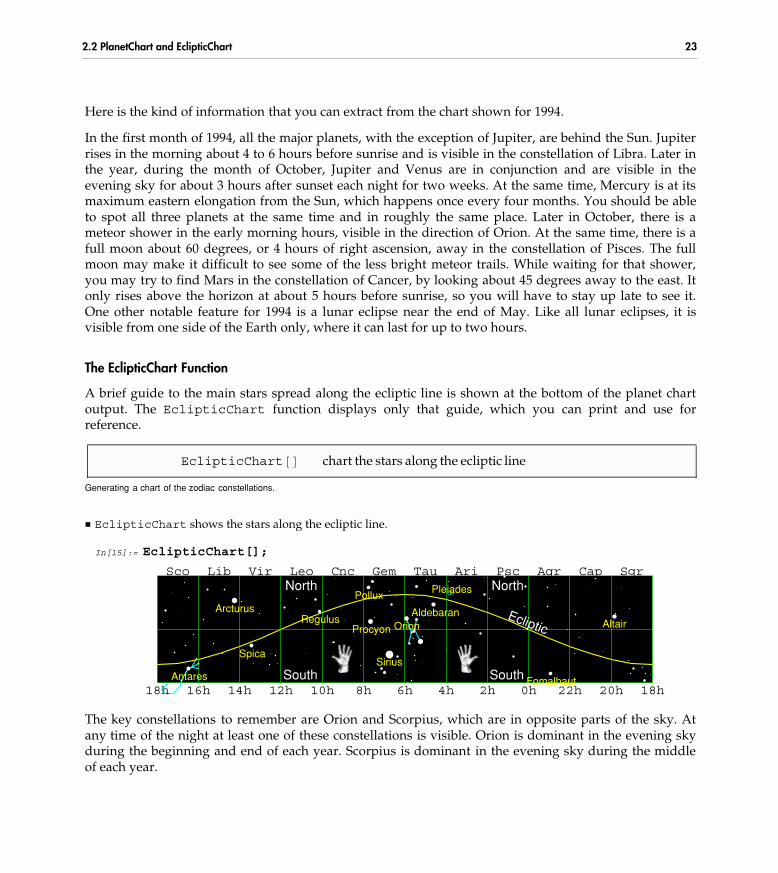
The EclipticChart Function
A brief guide to the main stars spread along the ecliptic line is shown at the bottom of the planet chartoutput. The EclipticChart function displays only that guide, which you can print and use forreference.
EclipticChart�� chart the stars along the ecliptic line
Generating a chart of the zodiac constellations.
� EclipticChart shows the stars along the ecliptic line.
In[15]:= EclipticChart[];
Sirius
Arcturus
Procyon Orion AltairAldebaran
Antares
Spica
Pollux
Fomalhaut
Regulus
PleiadesNorth North
South South
Ecliptic
18h
Sco
16h
Lib
14h
Vir
12h
Leo
10h
Cnc
8h
Gem
6h
Tau
4h
Ari
2h
Psc
0h
Aqr
22h
Cap
20h
Sgr
18h
The key constellations to remember are Orion and Scorpius, which are in opposite parts of the sky. Atany time of the night at least one of these constellations is visible. Orion is dominant in the evening skyduring the beginning and end of each year. Scorpius is dominant in the evening sky during the middleof each year.
2.2 PlanetChart and EclipticChart 23

� 2.3 The Planisphere Function
Planisphere produces either two or four graphic plates that you can use to build a planisphere for agiven geographic latitude. A planisphere is a device for determining which stars are above the localhorizon at any given hour for each day of the year.
Planisphere�� produce two plates needed to construct a planisphere
Fold �� True produce four plates for a more detailed planisphere
GeoLatitude �� latitude produce plates for a specific geographic latitude
Producing planispheric plates.
To construct the two-plate planisphere, print the first plate onto cardboard and the second plate onto atransparency. Then rivet the plates together at the center, which is marked with a small red circle. Trimthe plates to the outer circle. You may also want to glue a graphic generated by OuterPlanetChart tothe back of the planisphere. The OuterPlanetChart function is discussed in Section 5.5.
A two-plate planisphere is suitable for use in latitudes greater than 30 degrees north or south of theequator. There is, additionally, a four-plate planisphere suitable for latitudes less than 45 degrees northor south. If your latitude is between 30 and 45 degrees north or south, you can use either of the twostyles. To generate the four-plate planisphere, use the option setting Fold -> True. Construction ofthe four-plate planisphere is similar to the two-plate planisphere except that the second set of two platesgoes on the back of the first set of two plates, and there is no need to use the OuterPlanetChartgraphic. The four-plate planisphere produces a more detailed and accurate representation of the skythan the two-plate planisphere. It is, however, more difficult to construct, as additional gluing andcutting is required.
24 2. Basic Functions

� This displays the two planisphere plates needed for latitude -38 degrees in the southern hemisphere. By default, stars with magnitude less than 3.5 are not displayed, but you can changed this using the option MagnitudeRange.
In[16]:= Planisphere[GeoLatitude -> -38*Degree, StarLabels -> True, RotateLabel -> False];
Psc
Ari
Tau Gem
Cnc
Leo
Vir
Lib
ScoSgr
Cap
Aqr
Sirius
Canopus
Arcturus
Vega
Capella
RigelProcyon
Achernar
Betelgeuse
Altair
Acrux
Aldebaran
Antares
Spica
Pollux
Fomalhaut
Deneb
RegulusAdhara
Castor
Pleiades
Glue to cardboard 38 South
Jan1Jan1520hFeb1
Feb15 22h
Mar1
Mar15
0h
Apr1
Apr15
2hMay1
May15 4h
Jun1Jun15
6hJul1
Jul15 8h
Aug1
Aug1510h
Sep1
Sep1512h
Oct1
Oct15
14h
Nov1
Nov1516h
Dec1
Dec1518h
2.3 Planisphere 25

HorizonHorizon38
Planisphereby Terry Robb
Copy to transparency 38 South
MidnightEv
enin
gMorning
N
South
WE
6am
5am
4am
3am 2am 1am 12am
11pm
10pm
9pm
8pm
12am 11pm10pm
9pm
8pm
7pm
6pm
5pm
4pm
3pm
2pm
1pmNoon11am
10am
9am
8am 7am
6am
5am
4am
3am
2am 1am
To align the planisphere, hold it above your head and orient the North and South points to thecorresponding true compass directions. The red circle, where the rivet is located, will point to yourcelestial pole, which is either north or south depending on your hemisphere. The cross in the middle ofthe second plate will represent the zenith point directly above your head, and the gray lines are 30degrees apart.
To use the planisphere, keep the front plate stationary, and rotate the back plate with the stars on it, sothat the month and day point to the desired hour on the front plate. Stars that are visible through thewindow in the front plate are the stars that are visible in the real sky at that time. Standard time isrepresented in the outer circle of hours and daylight-saving time in the inner circle.
On the back plate, the blue ring represents the ecliptic line along which all the planets and Moonapproximately move. To find a planet you can either scan along that line in the real sky to find an
26 2. Basic Functions

unfamiliar object, or you can use OuterPlanetChart to create a finder chart. The finder chart isdesigned to be glued to the very back of the planisphere for easy reference. Another way to locateplanets in the sky is to remember that planets do not twinkle, unlike stars, which do twinkle as a rule.
Labeled on the outer rim of the planisphere are the right ascension hour and the zodiac constellations.
Any of the options available to StarChart are available to Planisphere. However,MagnitudeRange -> {-Infinity, 3.5} is used by default in order to keep the star plate frombecoming too cluttered.
� 2.4 The SunRise and NewMoon Functions
Precise times for common solar and lunar events are provided by the SunRise, SunSet, NewMoon, andFullMoon functions.
SunRise�neardate� compute the precise time of sunrise on the day of neardate
SunSet�neardate� compute the precise time of sunset on the day of neardate
NewMoon�neardate� compute the precise date of the new moon nearest to neardate
FullMoon�neardate� compute the precise date of the full moon nearest to neardate
Determining the precise times of common events.
Sunrise and sunset times are computed according to your current location and time zone as setpreviously with SetLocation. The location used throughout this user’s guide is Melbourne, Australia.
� On 1993 November 17, sunrise at Melbourne is about 06:00 (or 6:00am).
In[17]:= SunRise[{1993,11,17}]
Out[17]= �1993, 11, 17, 6, 0, 25�
� Sunset is about 20:10 (or 8:10pm).
In[18]:= SunSet[{1993,11,17}]
Out[18]= �1993, 11, 17, 20, 9, 52�
The SunRise and SunSet functions take into account atmospheric refraction. When light passes alongthe horizon to reach you, it is refracted by about 0.5 degrees, so that sunrise occurs about two minutesearlier than the time you would expect from simple geometry. Similarly, sunset occurs about twominutes later. You can use the option Refract->False to suppress refraction.
Related functions are NewMoon and FullMoon.
2.4 SunRise and NewMoon 27

� The new moon nearest to 1993 November 17 occurs on November 14.
In[19]:= NewMoon[{1993,11,17}]
Out[19]= �1993, 11, 14, 8, 35, 45�
� The nearest full moon occurs fifteen days later on November 29.
In[20]:= FullMoon[{1993,11,17}]
Out[20]= �1993, 11, 29, 17, 32, 51�
All the dates and times returned are accurate to within one minute.
As with all the functions in Scientific Astronomer, if you omit the date or near date argument, the currentdate (as calculated from Date[]) is always used. Thus, SunSet[] returns the time when the Sun willset today, and FullMoon[] returns the date of the nearest full moon.
You can use the NewMoon function to calculate the date of the Chinese New Year. As a general rule,Chinese New Year begins on new moon nearest to February 4 in any given year. Thus, a definition isChineseNewYear[year_] := NewMoon[{year, 2, 4}].
A related event is a Harvest Moon, which occurs on the day of a full moon nearest the northernautumnal equinox. On the evening of a Harvest Moon the Sun sets directly in the west at the same timeas a full moon rises in the east, thus extending the light at the end of the day. This symmetry greatlyimpressed ancient civilizations, many of which supposedly used the extra light to harvest crops. Moreoften though it was used as the time of a celebration. A definition is HarvestMoon[year_] :=FullMoon[{year, 9, 23}].
Related functions, which are built into Scientific Astronomer, include VernalEquinox[date],AutumnalEquinox[date], SummerSolstice[date], and WinterSolstice[date].
� 2.5 The BestView and InterestingObjects Functions
BestView is used to find when a planet, or any other object, is in a good viewing position relative to theSun. This occurs when the object is furthest from the Sun in relation to your viewing angle.
BestView�object, neardate� return some event dates, nearest to neardate,at which the object is at its best viewing condition
BestView�object� return some event dates nearest the current value of Date��
Determining the best viewing times for specified objects.
For the inner planets Mercury and Venus, the event dates are the evening and morning apparitions,which indicate when the planet appears in the evening or morning sky. For outer planets such as Mars,Jupiter, and Saturn, the event date is the time of opposition, which indicates when the planet is opposite
28 2. Basic Functions

in the sky to the Sun. For low-orbit Earth satellites, the event date is the transit visible time, whichindicates when the satellite is visible above the horizon and is making a transit overhead. For otherobjects, such as stars and constellations, the event date is simply the transit time at which the objectcrosses the local meridian line.
�Opposition �� date� event date for an outer planet, such as Mars, Jupiter or Saturn
�EveningApparition �� date, MorningApparition �� date�
event dates for the inner planets Mercury and Venus
�TransitVisible �� date� event date for a low-orbit Earth satellite
�Transit �� date� event date for other objects, such as stars
Event dates returned by BestView.
A typical use of BestView is to determine when, for instance, Mars is next in opposition.
� This shows that Mars reaches opposition on 1993 January 8.
In[21]:= BestView[Mars, {1993,11,17}]
Out[21]= �Opposition � �1993, 1, 8��
During an opposition, Mars is in the opposite direction to the Sun and consequently the orbits of Earthand Mars are close together. An opposition is a very good time to view Mars as it is at its largestapparent size. Every seventh opposition of Mars is particularly favorable as during those oppositions itis closer than normal to Earth. Mars oppositions are listed in Appendix A.11. In general, when anyplanet is in opposition, it is visible all night because it rises when the Sun sets, and sets when the Sunrises.
A planet is visible primarily in the morning sky before opposition, and in the evening sky afteropposition. Retrograde motion also occurs around the opposition event date. In the case of Mars,retrograde motion lasts about 10 weeks and reverses 15 degrees in the sky. For Jupiter, retrogrademotion lasts about 16 weeks and reverses 10 degrees. For Saturn, retrograde motion lasts about 20 weeksand reverses only 7 degrees.
Similarly, you can use BestView to find some good viewing dates for Mercury.
� The inner planet Mercury is visible in the evening sky around 1993 October 14 and in the morning sky around 1993 November 23.
In[22]:= BestView[Mercury, {1993,11,17}]
Out[22]= �EveningApparition � �1993, 10, 14�, MorningApparition � �1993, 11, 23��
Mercury is a particularly difficult planet to see because it is rarely in a good viewing position.BestView gives you the optimal dates to view it.
When an inner planet is at its greatest elongation east of the Sun as viewed from Earth, it is at its highestpoint in the evening sky just after dusk; at this time the planet is said to be making an evening
2.5 BestView and InterestingObjects 29

apparition. The planet is also furthest from the glare of the Sun, so the time of an evening apparition isthe best time for viewing the planet. Before an evening apparition, the planet is visible in the eveningsky, whereas after the evening apparition, it quickly moves toward the Sun to reappear later in themorning sky.
Once you have determined an evening apparition date for Mercury, try searching the western sky justafter dusk. The best evening apparitions are in spring. You should start searching for Mercury about 40minutes after sunset, and you can give up by about 70 minutes after sunset. Similarly, once you havedetermined a morning apparition date for Mercury, try searching the eastern sky just before dawn.
Viewing Asteroids
Only one asteroid is visible with the naked eye, and it can only be seen during opposition when it is atits closest and brightest. BestView allows you to find the date.
� This shows that Vesta reaches opposition on 1993 August 28.
In[23]:= BestView[Vesta, {1993,11,17}]
Out[23]= �Opposition � �1993, 8, 28��
� A call to Ephemeris on the opposition date determines the circumstances of the event. You can see that Vesta is 180 degrees from the Sun, and so it is indeed in opposition. Its apparent magnitude is 5.6, which is just visible to the naked eye under reasonable conditions.
In[24]:= Ephemeris[Vesta, Opposition /. %]
Vesta������������������������������������������Date Time: 1993�Aug�28 00:00:00 �GMT�11�
Geo�place: 145°00'E, 37°48'S �Earth.�
������� For Date, Geo�place: �������������Rising: 18:37 �Sunrise: 07:53�
Setting: 08:43 �Sunset: 18:50�
������� For Date Time, Geo�place: ��������Azimuth: 55°43' �NorthEast compass�
Altitude: 61°04' �Above the horizon�
������� For Date Time: �������������������Elongation: �179°07' �Morning sky. 100%�
Distance: 1.31 AU �Magnitude: �5.6�
������� For Date Time: �������������������Ascension: 22h43.0m �Aquarius 341°�
Declination: �18°43' �Ecliptic � 9°48'�
������������������������������������������
Out[24]= �EphemerisData�
30 2. Basic Functions

Viewing Stars and Satellites
BestView can also be applied to stars, in which case it returns a transit date that is the precise time atwhich the star crosses the local meridian line.
� BestView shows that the star Sirius crosses the local meridian at 04:22.
In[25]:= BestView[Sirius, {1993,11,17}]
Out[25]= �Transit � �1993, 11, 17, 4, 22, 26��
The local meridian is the great circle that starts at the point on the horizon directly south of your location,and passes up through the zenith and then down to the point on the horizon directly north of yourlocation. It also continues down to the nadir point directly below you, but that half of the meridian is notvisible. The north and south celestial poles are fixed points on your local meridian, although one of thecelestial poles is not visible below the horizon.
All stars cross your local meridian twice every day, once at a maximum angle above the horizon, andonce at a minimum angle, usually below the horizon. The transit date is the time of the maximumcrossing and is, therefore, a good time to view an object.
Another particularly useful application of BestView allows you to determine when a low-orbit satelliteis visible. In this case a transit visible event date is returned.
When a low-orbit Earth satellite is crossing the local meridian line and is illuminated by the Sun but theviewer location is still in darkness, the satellite is said to be transit visible. This is a fairly rare event, asmost satellites are only a few hundred kilometers above the Earth’s surface, and hence normallyeclipsed by the Sun when the Earth’s surface is in darkness. However, there is a very small window,approximately five minutes wide, when the satellite becomes transit visible.
More details on transit visible event dates are given in Section 7.2.
The InterestingObjects Function
InterestingObjects is a function related to BestView. The BestView function determines a timewhen an object is in a good viewing circumstance; InterestingObjects takes the inverse approachand returns all interesting objects that are visible at a specified time.
InterestingObjects�date� list all the interesting objects, such as galaxies, nebulae,clusters, as well as planets, constellations, and brightstars, that are above the local horizon
Altitude �� altitude minimum altitude to begin the search; default is15 Degree
Finding interesting objects above the horizon.
2.5 BestView and InterestingObjects 31

By default, only objects more than 15 degrees above the local horizon are returned. The Altitudeoption lets you set the lowest altitude above the local horizon to begin the search.
InterestingObjects searches for all planets as far out as Uranus, plus a few asteroids, severaldominant constellations, and many bright stars. It also searches through a long list of bright clusters,nebulae, and galaxies. In each case it returns the brightest objects in each category and sorts themaccording to apparent magnitude.
� Here is a list of the dominant objects above the horizon for Melbourne at 22:00 on 1995 December 1.
In[26]:= Print /@ InterestingObjects[{1995,12,1,22,0,0}];
Planets � �Moon, Saturn, Uranus�
Constellations � �Orion, CanisMajor, Pegasus, Carina�
Stars � �Sirius, Canopus, Rigel, Achernar, Aldebaran, Fomalhaut, Adhara�
Galaxies � �LargeMagellanicCloudGalaxy, SmallMagellanicCloudGalaxy,TriangulumGalaxy, SilverCoinGalaxy, CigarGalaxy, NGC300Galaxy�
Nebulae � �TarantulaNebula, OrionNebula, HelixNebula, CometNebula, SaturnNebula�
Clusters � �HyadesCluster, PleiadesCluster, ThetaCarinaeCluster, OmicronVelorumCluster,NGC2451Cluster, NGC2516Cluster, Tucanae47Cluster, TauCanisMajorisCluster,NGC3114Cluster, M41Cluster, TurquoiseOrbCluster�
� This searches for all the interesting objects more than 30 degrees above the local horizon. It shows that the Moon and Saturn are above the local horizon. It also shows that there are no dominant constellations at this time, although from the earlier output you can conclude that Orion, Canis Major, and Pegasus are low on the horizon. The brightest stars are Canopus, Achernar, and Fomalhaut.
In[27]:= Print /@ InterestingObjects[{1995,12,1,22,0,0}, Altitude -> 30*Degree];
Planets � �Moon, Saturn�
Constellations � ��
Stars � �Canopus, Achernar, Fomalhaut�
Galaxies � �LargeMagellanicCloudGalaxy, SmallMagellanicCloudGalaxy,SilverCoinGalaxy, CigarGalaxy, NGC300Galaxy�
Nebulae � �TarantulaNebula, HelixNebula, CometNebula�
Clusters � �Tucanae47Cluster, TurquoiseOrbCluster�
Some interesting open clusters that are built into Scientific Astronomer include ThetaCarinaeCluster,a 2nd magnitude cluster easily visible to the naked eye; PtolemysCluster, a large 3rd magnitudecluster in Scorpius separated by only 4 degrees from the 4th magnitude ButterflyCluster;JewelBoxCluster, a very colorful 4th magnitude cluster inside the Southern Cross; and
32 2. Basic Functions

WildDuckCluster, one of the best open clusters, visible in binoculars as a 6th magnitude fuzzy patchin Scutum.
Two of the many globular clusters built into Scientific Astronomer are OmegaCentauriCluster, easilythe finest globular cluster and visible to the naked eye at 4th magnitude; and HerculesCluster, thebrightest globular cluster visible from the northern hemisphere, at 6th magnitude.
Some notable diffuse nebulae built into Scientific Astronomer include OrionNebula, a naked-eyeemission nebula of 4th magnitude, greenish swirls visible in binoculars; EtaCarinaeNebula, a 6thmagnitude emission nebula and the largest diffuse nebula in the sky; and OmegaNebula, a 6thmagnitude red emission nebula in Sagittarius.
Notable planetary nebulae built into Scientific Astronomer include HelixNebula, the brightest planetarynebula at 6th magnitude in Aquarius; DumbbellNebula, a large 7th magnitude planetary nebulae inVulpecula, 0.25 degrees in diameter and green in color; CatseyeNebula, an 8th magnitude green andred planetary in Draco, looks like a cat's eye; and RingNebula, a 9th magnitude planetary in Lyra,separated by 7 degrees from the star Vega.
Many bright galaxies are also built into Scientific Astronomer. The list includes the 3rd magnitudeAndromedaGalaxy and the 7th magnitude CentaurusGalaxy. At 2.2 million light years theAndromeda Galaxy is the furthest object visible to the naked eye.
The lists BrightClusters, BrightNebulae, and BrightGalaxies contain many of thesepredefined deep sky objects that are built into Scientific Astronomer.
� BrightClusters gives a list of all the bright clusters, both open and globular, used by InterestingObjects. The list is sorted by apparent magnitude.
In[28]:= BrightClusters
Out[28]= �HyadesCluster, PleiadesCluster,ThetaCarinaeCluster, OmicronVelorumCluster,NGC6231Cluster, NGC2451Cluster, NGC3532Cluster, BeehiveCluster,PtolemysCluster, OmegaCentauriCluster, NGC2516Cluster,ChristmasTreeCluster, Tucanae47Cluster, TauCanisMajorisCluster,NGC3114Cluster, JewelBoxCluster, ButterflyCluster, IC4665Cluster,DoubleCluster, IC2581Cluster, NGC884Cluster, M47Cluster,M41Cluster, LambdaCentauriCluster, M39Cluster, NGC2244Cluster,M22Cluster, TurquoiseOrbCluster, WildDuckCluster, HerculesCluster�
2.5 BestView and InterestingObjects 33

� BrightNebulae lists all the bright nebulae, both diffuse and planetary.
In[29]:= BrightNebulae
Out[29]= �CoalSackNebula, TarantulaNebula,OrionNebula, LagoonNebula, RosetteNebula, FlamingStarNebula,EtaCarinaeNebula, NorthAmericaNebula, EagleNebula, OmegaNebula,TrifidNebula, HelixNebula, KeyholeNebula, CometNebula,DumbbellNebula, EightBurstNebula, CatseyeNebula, SaturnNebula,CrabNebula, UranusNebula, EskimoNebula, GhostOfJupiterNebula,BlinkingNebula, RingNebula�
� BrightGalaxies lists all the bright galaxies.
In[30]:= BrightGalaxies
Out[30]= �LargeMagellanicCloudGalaxy, SmallMagellanicCloudGalaxy,AndromedaGalaxy, TriangulumGalaxy, CentaurusGalaxy,SilverCoinGalaxy, BodesGalaxy, M110Galaxy, CigarGalaxy,M32Galaxy, SombreroGalaxy, WhirlpoolGalaxy, BlackeyeGalaxy,SouthernPinwheelGalaxy, VirgoGalaxy, NGC300Galaxy, M94Galaxy,PinwheelGalaxy�
34 2. Basic Functions

3. Coordinate FunctionsA system of coordinates is needed to represent the position of any object in space. This chapter discussesthe systems that are built into Scientific Astronomer.
Coordinate Systems
The Earth’s equatorial plane, when extended out into the sky, forms a great circle known as the celestialequator. The Sun moves along another great circle known as the ecliptic, which, due to the tilt of theEarth’s axis, is inclined to the celestial equator by an angle of about 23.5 degrees. These two great circlesintersect at two points known as equinoxes. One is called the vernal equinox and is the position of theSun at about March 21 of each year. The other is the autumnal equinox.
You can use the celestial equator and the vernal equinox to define a coordinate system known ascelestial coordinates, or equator coordinates. The equator coordinates system specifies the position of anobject by its right ascension and declination. Right ascension measures the angle, in hours of time, fromthe vernal equinox along the celestial equator; declination measures the angle north of the celestialequator. Stars have fixed equator coordinates, unlike the planets, which continually wander through thecelestial sphere, although always staying near the ecliptic. Sirius, the brightest star, has a fixed rightascension of 6h45m and a declination of -16°43'. The EquatorCoordinates function finds the equatorcoordinates of an object (such as a planet, the Moon, the Sun, or a star) on a given date.
Equator coordinates are useful in conjunction with star charts. There is, however, another more naturalcoordinate system that is useful out in the field and is based on the horizon. It is known as alt-azicoordinates, or more commonly as horizon coordinates.
Horizon coordinates specifies the position of an object by its azimuth and altitude. Azimuth measuresthe compass angle around the local horizon with 0 degrees being north and 90 degrees being east, andaltitude measures the angle above the local horizon with +90 degrees being overhead and -90 degreesbeing an unviewable point directly below the observer. Apart from geo-stationary satellites, no objectnormally has fixed horizon coordinates because the local horizon constantly changes throughout thenight. The HorizonCoordinates function finds the horizon coordinates of an object on a given date.
Yet another coordinate system is known as ecliptic coordinates. This system specifies the position of anobject by its ecliptic longitude and latitude. Ecliptic longitude measures the angle around the plane ofthe Earth’s orbit, with 0 degrees being the so-called first point in Aries. Ecliptic latitude measures theangle above the plane of the ecliptic. The EclipticCoordinates function finds the eclipticcoordinates of an object on a given date.
Coordinate Systems 35

Complications
The Earth’s axis gyrates around the pole of the ecliptic in a period of about 25,800 years. This effect,known as precession, can shift the celestial coordinates of objects by a few minutes of arc over severalyears. Stars, therefore, are not completely fixed on the celestial sphere, and the published celestialcoordinates assigned to each star are valid only for a specified epoch, usually taken as 1950 January 1 or2000 January 1. Most functions in Scientific Astronomer accept the option Epoch to let you choosesomething other than the current epoch.
Setting Your Site Location
As normal, before you use Scientific Astronomer, you must load the package and set your time zone andlocation on Earth.
� Load the package.
In[1]:= <<Astronomer`HomeSite`
Astronomer is Copyright �c� 1997 Stellar Software
� This sets your location to Melbourne, Australia.
In[2]:= SetLocation[GeoLongitude -> 145.0*Degree, GeoLatitude -> -37.8*Degree, GeoAltitude -> 0.0*KiloMeter, TimeZone -> 11];
� 3.1 The EquatorCoordinates Function
Equator coordinates are useful in conjunction with star charts.
EquatorCoordinates�object, date�
compute the right ascension, declination, and distanceof the object on the given date
EquatorCoordinates�object� compute the equator coordinates using the current valueof Date��
EquatorCoordinates�horizoncoords, date�convert the horizoncoords for the current location and dateinto equator coordinates
Calculating an object’s position in equator coordinates.
36 3. Coordinate Functions

EquatorCoordinates is typically applied to solar system objects such as Mars, Moon, and Io; starssuch as Sirius and Alpha.Centaurus; constellations such as Leo and UrsaMajor; special objectssuch as SouthCelestialPole and Zenith; and so on.
� Here you see that Mars is 21.6 degrees below the celestial equator, with a right ascension of 16.2 hours.
In[3]:= EquatorCoordinates[Mars, {1993,11,17,3,20,0}]
Out[3]= �Ascension � 16.2237 Hour, Declination � �21.6327 Degree,Distance � 2.45249 AU�
In the EquatorCoordinates output, the first rule is used to represent the right ascension of the object,which is the angle (in hours) around the celestial equator. The second rule is used to represent thedeclination, which is the angle above the celestial equator. An AU is the standard astronomical unit,which equals about 149,597,900km and is the mean distance between the Earth and the Sun. Hour isused to denote the unit of right ascension, and equals exactly 15 degrees of angle.
Distance is typically given in astronomical units, as this is a sensible unit for measurement within thesolar system. However, units of kilometers are used when a distance is less than 0.01 AU, and light yearsare used when a distance is greater than 1,000 AU. One light year equals about 63,240 AU.
� The Sun is 0.988773 AU distant from the Earth on the given date.
In[4]:= EquatorCoordinates[Sun, {1993,11,17,3,20,0}]
Out[4]= �Ascension � 15.4637 Hour, Declination � �18.8526 Degree,Distance � 0.988773 AU�
� The distance to the Moon is 373,502 kilometers (or 0.00253 AU) on the given date.
In[5]:= EquatorCoordinates[Moon, {1993,11,17,3,20,0}]
Out[5]= �Ascension � 18.1145 Hour, Declination � �20.9029 Degree,Distance � 373502. KiloMeter�
� The ascension, declination, and distance of the Moon is now slightly different than in the previous call.
In[6]:= EquatorCoordinates[Moon, {1993,11,17,3,20,0}, ViewPoint -> TopoCentric]
Out[6]= �Ascension � 18.1089 Hour, Declination � �20.0767 Degree,Distance � 376825. KiloMeter�
You can use the option setting ViewPoint -> object to specify any viewpoint. The default is the centerof the Earth (i.e., Earth), but you can specify any other object. For instance, TopoCentric is used tospecify the point on the surface of the Earth where you previously set your location.
3.1 EquatorCoordinates 37

With a TopoCentric viewpoint, the position of the Moon will appear slightly displaced relative to theposition obtained using the default Earth viewpoint. For most objects, which are much further awaythan the Moon, it does not matter if you use TopoCentric or Earth as the viewpoint.
You can also find the equator coordinates of a star. The syntax for specifying a star name is the dotnotation star.constellation, although the brightest 25 stars have been given aliases, so, for example, youcan use Sirius, Canopus, and Polaris as star names.
Stars have fixed equator coordinates–that is, they do not change with time. (Actually they do change alittle due to the precession of the Earth’s axis, but the effect is very small. Use the option Epoch to seethe effect.)
� Here are the fixed equator coordinates of the star Α (alpha) Centauri.
In[7]:= EquatorCoordinates[Alpha.Centaurus, {1993,11,17,3,20,0}]
Out[7]= �Ascension � 14.6522 Hour, Declination � �60.8038 Degree,Distance � 4.3 LightYear�
� This gives the equator coordinates of the point currently 30 degrees above the horizon and 60 degrees east of north on the given date.
In[8]:= EquatorCoordinates[{Azimuth -> 60*Degree, Altitude -> 30*Degree}, {1993,11,17,3,20,0}]
Out[8]= �Ascension � 8.95884 Hour, Declination � 2.04553 Degree�
Allowing for Precession
The option Epoch is available in many functions, including EquatorCoordinates . The default settingis Epoch -> Automatic, which specifies the current epoch for the plane of the Earth’s equator.However, you can use, say, Epoch -> 2000.0 to have ascension and declination returned relative tothe equator at epoch year 2000.
EquatorCoordinates�object, date, Epoch �� epoch�
compute the equator coordinates relative to a given epoch year
Allowing for the effect of precession.
Precession causes the plane of the equator to rotate about 50 arc-seconds per year, and this precessionmakes an epoch specification necessary.
38 3. Coordinate Functions

� Use Epoch to find the epoch 2000.0 coordinates of the star Α (alpha) Centauri.
In[9]:= EquatorCoordinates[Alpha.Centaurus, Epoch->2000.0]
Out[9]= �Ascension � 14.66 Hour, Declination � �60.83 Degree,Distance � 4.3 LightYear�
� The numbers are very slightly different for the epoch 1950.0 coordinates.
In[10]:= EquatorCoordinates[Alpha.Centaurus, Epoch->1950.0]
Out[10]= �Ascension � 14.5963 Hour, Declination � �60.6149 Degree,Distance � 4.3 LightYear�
The EclipticCoordinates Function
Equator coordinates measure the position of an object relative to the plane passing through the Earth’sequator. Ecliptic coordinates, in contrast, measure the position relative to the plane of the Earth’s orbit.The two planes are tilted by just 23.5 degrees, and so the coordinate systems are closely related.
EclipticCoordinates�object, date�
return the ecliptic longitude, ecliptic latitude,and distance of the object on the given date
ViewPoint �� Sun coordinates relative to the Sun; default is Earth
Calculating an objects position in ecliptic coordinates.
In the EclipticCoordinates output, the first rule is used to represent the value of the eclipticlongitude of an object. The value will be very close to the right ascension of the object. Similarly, thesecond rule is used to represent the value of the ecliptic latitude. The value will be close (within 23.5degrees) to the declination of the object.
� By definition the ecliptic latitude of the Sun is zero.
In[11]:= EclipticCoordinates[Sun, {1993,11,17,3,20,0}]
Out[11]= �EclipticLongitude � 234.324 Degree, EclipticLatitude � 0. Degree,Distance � 0.988773 AU�
� On the same date, Mars is just 0.44 degrees below the ecliptic line. It has an ecliptic longitude of 245 degrees.
In[12]:= EclipticCoordinates[Mars, {1993,11,17,3,20,0}]
Out[12]= �EclipticLongitude � 245.362 Degree,EclipticLatitude � �0.442809 Degree, Distance � 2.45249 AU�
3.1 EquatorCoordinates 39

� 3.2 The HorizonCoordinates Function
Horizon coordinates are useful when you are out in the field. The HorizonCoordinates functioncomputes the position of an object relative to the local horizon. The output, therefore, depends on yourgeographic location on Earth.
HorizonCoordinates�object, date�
compute the azimuth, altitude, and distance of the objecton the given date
HorizonCoordinates�object� compute the horizon coordinates using the current valueof Date��
HorizonCoordinates�equatorcoords, date�
convert the equatorcoords into horizon coordinates forthe current location and date
Calculating an object’s position in horizon coordinates.
� Mars, on the given date and time, is 26.9 degrees below the horizon and 156 degrees east of north, which is approximately south-southeast.
In[13]:= HorizonCoordinates[Mars, {1993,11,17,3,20,0}]
Out[13]= �Azimuth � 156.591 Degree, Altitude � �26.9461 Degree,Distance � 2.45249 AU�
In the HorizonCoordinates output, the first rule is used to represent the compass angle around thehorizon, and the second rule is used to represent the angle above the horizon. A negative altitude meansthe object is currently below the local horizon. Azimuth is defined so that 0 degrees is the directionnorth and 90 degrees is the direction east.
HorizonCoordinates can be applied to stars and other objects as normal.
� Discover the current horizon coordinates of the star Α (alpha) Centauri using HorizonCoordinates.
In[14]:= HorizonCoordinates[Alpha.Centaurus, {1993,11,17,3,20,0}]
Out[14]= �Azimuth � 158.658 Degree, Altitude � 15.4941 Degree,Distance � 4.3 LightYear�
40 3. Coordinate Functions

� This gives the current azimuth and altitude of the fixed point on the celestial sphere with an ascension of 6 hours and a declination of 30 degrees.
In[15]:= HorizonCoordinates[{Ascension -> 6*Hour, Declination -> 30*Degree}, {1993,11,17,3,20,0}]
Out[15]= �Azimuth � 3.97086 Degree, Altitude � 22.0836 Degree�
The Refract Function
A function related to HorizonCoordinates is Refract. Refract adds an atmospheric refractioncorrection to horizon coordinates. Atmospheric refraction can amount to about 0.5 degrees for an objectclose to the horizon, but requires a very minor correction for objects well above the horizon.
Refract�horizoncoords� convert the true horizoncoords into apparent horizoncoordinates by adding an atmospheric refraction correction
Allowing for the effect of atmospheric refraction.
SunRise and SunSet correctly take into account atmospheric refraction. However, this means that thetrue horizon coordinates of the Sun place it approximately half a degree below the horizon at sunrise orsunset. To correct this for refraction, you can apply Refract.
Refraction has its strongest effect on horizon coordinates with an altitude near zero, in which case itadds about half a degree to that altitude. When horizon coordinates reach about 15 degrees of altitude,refraction has very little effect.
� The true position of the Sun is 0.55 degrees below the horizon at sunset.
In[16]:= HorizonCoordinates[Sun, SunSet[], ViewPoint -> TopoCentric]
Out[16]= �Azimuth � 253.988 Degree, Altitude � �0.549684 Degree,Distance � 0.994219 AU�
� The atmospherically refracted position of the Sun at sunset lies almost exactly on the horizon, with an altitude of just -0.002 degrees, which is where it should be at that time.
In[17]:= HorizonCoordinates[Sun, SunSet[], ViewPoint -> TopoCentric]//Refract
Out[17]= �Azimuth � 253.988 Degree, Altitude � �0.00224249 Degree,Distance � 0.994219 AU�
3.2 HorizonCoordinates 41

� 3.3 The Coordinates Function
Coordinates is useful for producing various three-dimensional plots.
Coordinates�object, date� return the x, y, z coordinates �in astronomical units� ofthe object on the given date
ViewPoint �� planet coordinates relative to the given planet
Calculating an object’s position in x,y,z coordinates.
The three-dimensional coordinate system used by Coordinates is aligned so that the z coordinate isperpendicular to the plane of the Earth’s orbit about the Sun, and the x coordinate points in the directionof the 0h line of right ascension. For historical reasons, the 0h line is called the first point of Aries, eventhough the point is currently in the direction of Pisces. Several thousand years ago the 0h line of rightascension was in Aries, but precession has been slowly moving it, so that now it lies in Pisces and ismoving into Aquarius.
Output position is given in astronomical units.
� The Coordinates function gives you the x,y,z coordinates of Mars on the given date.
In[18]:= Coordinates[Mars, {1993,11,17,3,20,0}]
Out[18]= ��1.02237, �2.22915, �0.0189538�
� Here Coordinates gives the x,y,z coordinates of the Moon.
In[19]:= Coordinates[Moon, {1993,11,17,3,20,0}]
Out[19]= �0.0000699065, �0.0024933, 0.000110107�
A default viewpoint of Earth is used here, but any viewpoint is allowed.
42 3. Coordinate Functions

� This plots the orbit of Mercury as viewed from the Sun. You can see the expected elliptical orbit with the Sun centered at one focal point. Observe the somewhat eccentric shape of the ellipse.
In[20]:= ListPlot[ Table[Take[Coordinates[Mercury, {1993,1,d}, ViewPoint -> Sun], 2], {d, 1, 89, 2}], PlotJoined -> True, AspectRatio -> 1];
-0.4-0.3-0.2-0.1 0.1 0.2 0.3
-0.4
-0.2
0.2
3.3 Coordinates 43

� Using Earth as the viewpoint, it becomes clear that Mercury makes roughly three close approaches to the Earth each year.
In[21]:= ListPlot[ Table[Take[Coordinates[Mercury, {1993,1,d}, ViewPoint -> Earth], 2], {d, 1, 366, 5}], PlotJoined -> True, AspectRatio -> 1];
-1 -0.5 0.5 1
-1.5
-1
-0.5
0.5
1
� 3.4 The JupiterCoordinates Function
JupiterCoordinates determines the precise positions of the main moons of Jupiter. It can alsodetermine the positions of various cloud features on the surface of Jupiter, such as the Great Red Spot.
JupiterCoordinates�moon, date�
return the relative x, y, z coordinates �in Jovian radii� ofa Galilean moon
JupiterCoordinates�moon� return the relative x, y, z coordinates using the currentvalue of Date��
Calculating position in Jovian coordinates.
The first coordinate returned by JupiterCoordinates indicates the number of Jovian radii east (inthe right ascension direction) of Jupiter. The second coordinate is the number of Jovian radii north (inthe declination direction) of Jupiter. The third coordinate is the object’s distance from Jupiter in Jovianradii in the direction away from Earth.
44 3. Coordinate Functions

You can apply JupiterCoordinates to the four Galilean moons Io, Europa, Ganymede, and Callisto.You can also apply the function to the Great Red Spot JupiterGreatRedSpot.
� Find the Jupiter coordinates of the moon Io on the given date.
In[22]:= JupiterCoordinates[Io, {1993,11,17,3,20,0}]
Out[22]= �3.0396, �0.247141, 5.03695�
� JupiterGreatRedSpot gives the Jupiter coordinates of the Great Red Spot on the same date.
In[23]:= JupiterCoordinates[JupiterGreatRedSpot, {1993,11,17,3,20,0}]
Out[23]= �0.0332883, �0.358368, 0.932987�
Remember that the position of the Great Red Spot is somewhat unpredictable. However, once itsposition, or Jovian longitude, is known on a particular date, it moves slowly relative to that positionover time.
$JupiterGreatRedSpotLongitude
global variable that can be set to the current Jovianlongitude of the Great Red Spot; default is –�40 Degree
Specifying the position of the Great Red Spot.
The Great Red Spot stays roughly fixed in the System II coordinate system of Jupiter, but over the yearsit slowly drifts. Apart from that drift, the spot moves around Jupiter about once every 9 hours 55minutes. Some values for $JupiterGreatRedSpotLongitude are -45° (June 1990), -33° (June 1992),-40° (June 1994), -41° (July 1994), -42° (July 1995), -49° (November 1995), -51° (September 1996), and -61°(November 1996). The default is -40°. You can sometimes obtain current values by consulting themagazine Sky & Telescope, published by Sky Publishing Corporation, Belmont, MA. Note that they usethe opposite direction than the one used here for the definition of positive Jovian longitude–that is, westis positive, rather than east–so you must remember to use the negative of these Jovian longitudes inScientific Astronomer.
3.4 JupiterCoordinates 45

Jupiter Coordinates
The central meridian of Jupiter is the semicircular line passing through the poles of Jupiter and thecenter of the disk as seen from Earth. Features on Jupiter rotate with respect to the central meridianroughly every 10 hours. The rotation rate is, however, latitude dependent, but it neatly splits into twosystems. System I is the equatorial belt with latitudes between +10 and -10 degrees. This system makes afull rotation in a period of about 9 hours 50 minutes 30 seconds, although System I is actually defined sothat the mean motion is exactly 877.90 degrees per day. System II consists of all latitudes outside SystemI. All features in this region complete a full rotation in a period of about 9 hours 55 minutes 40 seconds,although System II is defined so that the mean motion is exactly 870.27 degrees per day. The Great RedSpot is near the top of the southern portion of System II.
46 3. Coordinate Functions

4. Star Charting FunctionsFour main types of star charts are implemented in Scientific Astronomer. They are created by thefunctions RadialStarChart, ZenithStarChart, CompassStarChart, and StarChart. A fifth starcharting function is Planisphere.
Why Four Star Charts?
Each star charting function has its own advantages and disadvantages. For instance, StarChart worksquickly because it simply draws a direct map of the ascension and declination coordinates of each star.However, this function is really only suitable for charting close to the celestial equator, as there isconsiderable distortion near the celestial poles. To overcome this problem, RadialStarChart can beused.
RadialStarChart can plot any part of the sky with little or no distortion in the center of the chart.Some distortion may occur on the edges if the field of view is large. This function is slower thanStarChart because it has to transform the raw star positions as a function of the field of view. Onefeature of both StarChart and RadialStarChart is that they can zoom into small regions. They arenot good at encompassing large fields of view; the two global star chart functions are more useful in thiscase.
ZenithStarChart and CompassStarChart can plot only large global sections of the sky. They dothis in such a way as to minimize distortion as much as possible. With ZenithStarChart, the full skyabove the local horizon and up to the zenith point is displayed. There is little or no distortion in thecenter, which is the zenith point, but around the edges and along the horizon there is some stretching.CompassStarChart takes the opposite tack and has no distortion along the horizon, but in order to dothis it can display only one half of the sky above the horizon.
Setting Your Site Location
� Load the package.
In[1]:= <<Astronomer`HomeSite`
Astronomer is Copyright �c� 1997 Stellar Software
� This sets your location to Melbourne, Australia.
In[2]:= SetLocation[GeoLongitude -> 145.0*Degree, GeoLatitude -> -37.8*Degree, GeoAltitude -> 0.0*KiloMeter, TimeZone -> 11];
Why Four Star Charts? 47

Stars and Constellations
In EquatorCoordinates, HorizonCoordinates, and many other functions, you can specify a staras well as a planet, asteriod, or any other celestial object. Stars are specified using a dot notation toseparate star label and constellation name, that is, star.constellation. The sky is arbitrarily divided upinto a standard set of 88 constellations.
� Here is a list of the 88 constellations.
In[3]:= ?Constellation`*
Andromeda Cygnus OrionAntlia Delphinus PavoApus Dorado PegasusAquarius Draco PerseusAquila Equuleus PhoenixAra Eridanus PictorAries Fornax PiscesAuriga Gemini PiscisAustrinusBootes Grus PuppisCaelum Hercules PyxisCamelopardalis Horologium ReticulumCancer Hydra SagittaCanesVenatici Hydrus SagittariusCanisMajor Indus ScorpiusCanisMinor Lacerta SculptorCapricornus Leo ScutumCarina LeoMinor SerpensCassiopeia Lepus SextansCentaurus Libra TaurusCepheus Lupus TelescopiumCetus Lynx TriangulumChamaeleon Lyra TriangulumAustraleCircinus Mensa TucanaColumba Microscopium UrsaMajorComaBerenices Monoceros UrsaMinorCoronaAustralis Musca VelaCoronaBorealis Norma VirgoCorvus Octans VolansCrater Ophiuchus VulpeculaCrux
Prior to 1930, there was no agreement on constellation boundaries and names–different authors oftenused different systems. In 1930, astronomers decided to rationalize the system and have 88constellations and give them all Latin names. This internationally recognized system is used by ScientificAstronomer. In this system the popularly known Scorpio is referred to as Scorpius. Similarly the BigDipper is referred to as Ursa Major, which in Latin means Great Bear.
Within each constellation, individual stars are typically labeled with Greek letters. The letter Α (alpha) isusually, but not always, the brightest star in a given constellation. The convention for the full name of astar is to use the Greek letter followed by the possessive form of the constellation name. In Latin, thepossessive form of Centaurus is Centauri therefore the brightest star in the constellation of Centaurus isknown as Α (alpha) Centauri. In Scientific Astronomer, however, this star is referred to as
48 4. Star Charting Functions

Alpha.Centaurus–that is, the nonpossessive form of the constellation name is used and a dot is usedto separate star label and constellation name. Similarly, the brightest star in Ursa Major is Α (alpha)Ursae Majoris, but in Scientific Astronomer it is referred to as Alpha.UrsaMajor.
Bright Star Names
The 25 brightest stars are also given special names in Scientific Astronomer. For instance, there is Sirius,which is the same as Alpha.CanisMajor; and also Polaris, which is the same asAlpha.UrsaMinor.
As normal, basic information about an object is obtained by using the ? function.
� BrightStar is a Mathematica context that contains all the stars down to magnitude 1.5, but also includes Polaris at magnitude 2.02. Additionally, it includes the eclipsing variable star Algol and the wide double star Mizar.
In[4]:= ?BrightStar`*
Achernar Altair Canopus Mizar RigelAcrux Antares Capella Polaris RigilKentAdhara Arcturus Castor Pollux SiriusAgena Becrux Deneb Procyon SpicaAldebaran Bellatrix Fomalhaut Regulus VegaAlgol Betelgeuse Gacrux
� Sirius is an alias for Alpha.CanisMajor or Α (alpha) Canis Majoris.
In[5]:= ?Sirius
Sirius � Alpha.CanisMajor; Magnitude � �1.46
The SetStars Function
If you have your own list of stars, or you want to modify the current list of stars, you need to useSetStars.
SetStars�starlist� set the list of stars to be used
MagnitudeRange �� range a subset of the stars
Setting the stars to use in the package.
Each star in the star list should consist of a constellation name, star name, magnitude, ascension (indegrees, not hours), and declination (in degrees).
You rarely need to use this function, which simply sets a value for the list TheStars. Initially this list isset to the value of the list Stars300, but if you load <<Astronomer`Star3000`; then it is set toStars3000.Similarly, it can be set to Stars9000.You can use the option MagnitudeRange to filterout a subset of the stars.
Bright Star Names 49

� This loads 3,000 extra stars and automatically calls SetStars to make them available.
In[6]:= <<Astronomer`Star3000`
� 4.1 The StarChart Function
StarChart is used to show a rectangular section of the sky. Several other types of star charts areavailable, but this one is the fastest. Like all the other star chart functions in Scientific Astronomer,StarChart accepts a large number of options for producing a wide variety of output styles.
StarChart�object� plot a rectangular region of the sky centered on the object; thiscan be one of the 88 constellations or any other object,such as a star
StarChart���asc1, asc2�, �dec1, dec2���
plot a rectangular region of the sky with right ascensionbetween asc1 and asc2, and declination between dec1 and dec2
Plotting stars in a rectangular region.
Like most other functions, StarChart is typically applied to solar system objects such as Mars, Moon,and Io; stars such as Sirius and Alpha.Centaurus; constellations such as Leo and UrsaMajor;special objects such as SouthCelestialPole and Zenith; and so on.
50 4. Star Charting Functions

� The solid angle covered by this chart of the Scorpius constellation is about four times the area of your hand when held at arm’s length. The vertical axis indicates declination and the horizontal axis shows right ascension.
In[7]:= StarChart[Scorpius];
18h 17h 16h
�50
�45
�40
�35
�30
�25
�20
�15
In some of the star chart graphical output you may notice a blue line crossing the field of view. Thisrepresents the ecliptic, which is the precise line that the Sun moves along during the course of a year.The Moon and all the planets approximately move along this line, too, so the ecliptic is very important.All the 12 zodiac constellations are located near the ecliptic as well.
To switch off the line, you can use the Ecliptic -> False option. The default is Ecliptic ->True.
4.1 StarChart 51

All the star charts use thin green lines to join together some of the brighter stars to form theconstellations. By default, constellation outlines are drawn, but you can suppress them using the optionsetting Constellations -> False.
A feature of all the star charts is that you can, on appropriate front ends, hold down the � key, clickinside a graphic, and copy the pair of numbers representing the point where you clicked. That pair ofnumbers can then be used in other functions as if they were an object.
In the case of StarChart you can also hold down �-� and select a rectangle, and then copy thatpair of number pairs into another StarChart call. This allows you to interactively zoom into a smallerportion of the sky. (Note the �-� feature may not be available on all front ends.)
Suppose, for example, that you generate a large section of the sky that contains the constellation ofOrion. By using the �-�-select-and-copy feature you can place a rectangle around Orion to get abounding box that you can use as the argument in a subsequent StarChart call.
Bounding boxes are a pair of number pairs giving first the minimum and maximum x values, and thenthe minimum and maximum y values of the rectangle. An x range of {-108.818, -56.455}corresponds to a right ascension range of 7.25 hours (from +108.818/15) to 3.76 hours. Similarly, a yrange of {-22.091, 22.091} corresponds to a declination range of -22.09 degrees to +22.09 degrees.
52 4. Star Charting Functions

� In a chart zoomed into a smaller part of the sky, the �-�-select-and-copy feature is used in a previous StarChart graphic to get the bounding box that is used as the argument in this call.
In[8]:= StarChart[{{-108.818, -56.455}, {-22.091, 22.091}}];
7h 6h 5h 4h
�20
�15
�10
�5
0
5
10
15
20
4.1 StarChart 53

� A chart of the daytime sky near the constellation of Libra shows the Sun and the Moon superimposed. These are their positions 2 hours before the new moon nearest 1993 November 17, which occurs on 1993 November 14. The brown area on the upper left is the horizon, with the ground below it.
In[9]:= StarChart[Libra, NewMoon[{1993,11,17}]+{0,0,0,-2,0,0}, Planets -> All, Horizon -> True];
16h 15h 14h
�40
�35
�30
�25
�20
�15
�10
�5
54 4. Star Charting Functions

� Here is a chart of the constellation of Orion with constellation labeling and an equator coordinates mesh superimposed. Spectral colors of the stars are also shown. Betelgeuse is the orange-red star on the right shoulder, which is our left, of Orion. Of course, in the southern hemisphere it appears upside down. If you look at Orion in the actual sky you should have little trouble identifying the unusual color of Betelgeuse.
In[10]:= StarChart[Orion, ConstellationLabels -> True, Mesh -> True, StarColors -> True];
6h 5h
�15
�10
�5
0
5
10
15
20
Orion
Taurus
Star charts use black stars on a white background, because that is how you would typically print a chart.Sometimes, however, a more realistic rendering of the night sky is required. You can use the optionStarColors -> True to color the brighter stars according to their actual visual spectral color. In thiscase the background sky is rendered as black. The default is StarColors -> False.
4.1 StarChart 55

option name default value
RadialAngle 20 Degree the angular size of the chart
MagnitudeRange ��Infinity, Infinity� the range of star magnitudes
MagnitudeScale 1 the scale size of the star dots
Skyline �� a skyline along the horizon
Horizon False drawing of the horizon line
MilkyWay False drawing of an outline of theMilky Way
GalacticPlane False drawing of the plane of ourgalaxy
Ecliptic True drawing of the ecliptic line
Constellations True outlines for constellations
Planets None markings for the given planets
Stars True markings for stars
Clusters True markings for clusters
Nebulae True markings for nebulae
Galaxies False markings for galaxies
ConstellationLabels False labeling of constellations
PlanetLabels False labeling of planets
StarLabels False labeling of brighter stars
ClusterLabels False labeling of clusters
NebulaeLabels False labeling of nebulae
GalaxyLabels False labeling of galaxies
RotateLabel True rotated text for all labeling
StarColors False coloring of stars
Mesh False an equator coordinates mesh
Background Automatic background color of the chart
ViewVertical Automatic rotation of chart
Epilog �� graphics primitives to berendered after the main plot
Prolog �� graphics primitives to berendered before the main plot
Some of the options for StarChart, RadialStarChart, CompassStarChart, ZenithStarChart, and Planisphere.
56 4. Star Charting Functions

There are many other options to StarChart and the other star chart functions. To display stars on ablack sky you can use the option setting Background -> RGBColor[0,0,0], and to labelconstellations you can use ConstellationLabels -> True. Similarly, you can label planets,superimpose an equator coordinates mesh, and color stars according to their spectral colors.
By default, only the brightest 300 stars are used by StarChart and the other star chart functions, butyou can load extra stars such as those in the Star3000.m file, which includes the brightest 3,000 stars.You can artificially brighten or dim the stars by using the option MagnitudeScale.
Stars are drawn as small dots with a radius in proportion to their magnitude. You can use theMagnitudeScale option to increase the size of the dots if you decide they are too small. For example,to double the radius of the dots, use the setting MagnitudeScale -> 2. Similarly, you can use thesetting MagnitudeScale -> 0.3 to decrease the size of the dots. The default value is, of course,MagnitudeScale -> 1.
Sometimes, when you load extra stars from the Star3000.m or Star9000.m files, you may not wantto see all of these stars. In such a case, you can use the MagnitudeRange option with any star chartfunction to select the range of star magnitudes to be displayed.
The syntax is MagnitudeRange -> {min, max} or MagnitudeRange -> max. The default isMagnitudeRange -> {-Infinity, Infinity}, which means display stars of all magnitudes. Anoption value of MagnitudeRange -> 4.0 would request that only stars down to magnitude 4.0 bedisplayed.
� 4.2 The RadialStarChart Function
RadialStarChart is useful for displaying the relative layout of stars. You specify a direction and afield of view, and the appropriate graphic is returned.
RadialStarChart�object, date� plot a circle of the sky centered on the object on the given date
RadialStarChart�object� plot a circle of the sky using the current value of Date��
RadialStarChart�constellation� plot a circle of the sky centered on one of the 88 constellations
RadialStarChart�horizoncoords, date�
plot a circle of the sky centered on horizoncoords on the given date
Planets �� planets additional red dots for the position of the planets on thegiven date
RadialAngle �� angle a bigger or smaller field of view; default is 20 Degree
Plotting stars near a central point.
An advantage of RadialStarChart over StarChart is that it can produce a plot with much lessdistortion. No matter which direction in the celestial sphere you look, RadialStarChart gives you arelatively undistorted representation, whereas StarChart has considerable distortion near the celestialpoles.
4.2 RadialStarChart 57

As with the other star charts, green lines are used to highlight common constellations to aididentification. These lines can be switched off with the option setting Constellations -> False.
Many options are available with RadialStarChart.
� A chart looking in the direction of the north celestial pole shows the pole star Polaris in the center and the Big Dipper UrsaMajor to the left. The field of view is 50 degrees in angular radius, so the graphic is 100 degrees across.
In[11]:= RadialStarChart[NorthCelestialPole, RadialAngle -> 50*Degree];
12.0013 Hour 89.9826 Degree
RadialAngle: 50. Degree
58 4. Star Charting Functions

� RadialStarChart[Scorpius] creates a chart of the Scorpius constellation. The two special nine-dot symbols to the left of Scorpius are open star clusters. The bigger cluster is M7 and the much smaller one is M6, which is sometimes known as the Butterfly cluster. To remove star clusters use the option setting Clusters -> False.
In[12]:= RadialStarChart[Scorpius];
17. Hour �31. Degree
RadialAngle: 20. Degree
4.2 RadialStarChart 59

� This is a chart looking toward Venus at sunset. Note the use of the option setting Horizon -> True as well as the other options. The brown-colored curve at the bottom is the line of the local horizon, into which the yellow Sun is setting. At the very bottom the compass direction is written. The Sun, which is shown sitting directly on the horizon, obviously sets into the west.
In[13]:= RadialStarChart[Venus, SunSet[{1994,10,13}], RadialAngle -> 45*Degree, Planets -> All, PlanetLabels -> True, ConstellationLabels -> True, Horizon -> True, MagnitudeRange -> {-Infinity, 3.5}];
Ara
Centaurus
Circinus
Corvus
Crux
Libra
Lupus
Norma
Ophiuchus
ScorpiusTriangulumAustrale
Virgo
Sun
Mercury
VenusJupiter
Pluto
West
14.8993 Hour �23.9006 Degree
RadialAngle: 45. Degree
60 4. Star Charting Functions

You can project the line of the local horizon onto a star chart by using the Horizon -> True option.The Horizon option is applicable to StarChart and RadialStarChart, with the default beingHorizon -> False. Since the horizon changes with time, you need to supply a date to the star chartfunction.
When the Horizon -> True option is used in a RadialStarChart, the graphic is rotated so that thehorizon line is horizontal. This is not possible with the plain StarChart function, which has a morerigidly aligned coordinate system. In that function, the horizon line and the ground below it are coloredbrown.
Stars have generally fixed positions in the rotating sky and so are easy to display consistently in thevarious star charts. Planets, however, continually wander through the sky (although always near theecliptic) and so are not normally displayed in the star charts. To render planets in a star chart you can setthe Planets option to the value All, or to a list of planet names, or even to other objects. The default isPlanets -> None.
When planets are displayed you might have trouble identifying which planet is which. To remedy thisthe option PlanetLabels -> True is available to place labels below the planets. The default isPlanetLabels -> False.
Sometimes it is useful to have constellations labeled as well, since not all constellations are easilyidentifiable by sight. This is where the ConstellationLabels -> True option is useful. The defaultvalue is ConstellationLabels -> False.
By default, the background sky is white unless the StarColor option is set to True, in which case thebackground sky is black. If neither of these colors is suitable to you, then you can use the Backgroundoption. Whatever background color you choose, contrasting colors are used for stars. The Backgroundoption can be a CMYKColor, GrayLevel, Hue, or RGBColor directive. The default is Automatic,which chooses between GrayLevel[0] and GrayLevel[1] depending on whether StarColor isTrue or False.
There are many other options available to the star charts. For example, Mesh -> True superimposesan equator coordinates mesh. Mesh lines units are 1 hour of right ascension, and 15 degrees ofdeclination. Crosses are placed at the north and south celestial poles. To suppress the text around theedges use the option Text -> False.
4.2 RadialStarChart 61

� The Background and Mesh settings designate a blue background and a gray equator coordinates mesh in this star chart.
In[14]:= RadialStarChart[UrsaMinor, RadialAngle -> 40*Degree, Background -> RGBColor[0.1,0.1,1], Mesh -> True, ConstellationLabels -> True];
Camelopardalis
CanesVenatici
Cepheus
Draco
UrsaMajor
UrsaMinor
14. Hour 73. Degree
RadialAngle: 40. Degree
62 4. Star Charting Functions

� When you request star colors, a black background appears by default.
In[15]:= RadialStarChart[Crux, RadialAngle -> 40*Degree, Mesh -> True, StarColors -> True, ConstellationLabels -> True];
Antlia
Apus
Ara
Carina
Centaurus
Chamaeleon
Circinus
Crux
Lupus
Mensa
Musca
Norma
Octans
Pictor
TriangulumAustrale
Vela
Volans
12.5 Hour �61. Degree
RadialAngle: 40. Degree
As normal, you can look at any named object, such as Mars, Sirius, Leo, or Zenith, but it is alsopossible to look at a fixed point in the sky relative to the local horizon by using horizon coordinates. Forexample, RadialStarChart[{Azimuth -> 180*Degree, Altitude -> 20*Degree},{1993,11,17,3,20,0}]; generates a chart centered on the point directly south and 20 degrees up inthe sky. Similarly, you can use equator coordinates.
4.2 RadialStarChart 63

� 4.3 The CompassStarChart Function
CompassStarChart displays a global section of the sky. You specify a compass direction, and agraphic showing all the stars in that direction is displayed.
CompassStarChart�direction, date�
chart the star field in the compass direction, which canbe either North, South, East, West, or a compassangle in degrees, on the given date
CompassStarChart�direction� chart the star field using the current value of Date��
Plotting stars in half the sky.
Two CompassStarChart calls can be used to cover the entire sky above the local horizon.
At the top of the graphic, a cross is used to represent the zenith, which is the point directly above yourhead. The field of view is 180 degrees along the horizon and is shown as the brown line along thebottom. The blue line is the ecliptic, which can be removed using the option setting Ecliptic ->False.
As with other star chart functions, numerous options are available. The options are identical to those forStarChart. For instance, to add an equator coordinates mesh use Mesh -> True. To show the MilkyWay use MilkyWay -> True. Use the option Text -> False to suppress the text printed at the topleft and right edges of the graphic.
64 4. Star Charting Functions

� Observe the southern aspect of the sky above the horizon at 03:20 on 1993 November 17 as seen from Melbourne, Australia.
In[16]:= CompassStarChart[South, {1993,11,17,3,20,0}, Mesh -> True, StarColors -> True, MagnitudeRange -> 4.0];
East South West
Nov 17
03:20
Latitude
38 South
4.3 CompassStarChart 65

� This chart shows the northern aspect of the same sky.
In[17]:= CompassStarChart[North, {1993,11,17,3,20,0}, Mesh -> True, StarColors -> True, MagnitudeRange -> 4.0];
West North East
Nov 17
03:20
Latitude
38 South
66 4. Star Charting Functions

� The western aspect of the sky displays part of the Milky Way, which can be seen on both the right and the left. The blue line sweeping from the western horizon to a point above north is the ecliptic.
In[18]:= CompassStarChart[West, {1993,11,17,3,20,0}, Mesh -> True, MilkyWay -> True, MagnitudeRange -> 4.0];
South West North
Nov 17
03:20
Latitude
38 South
Note the usefulness of the option Mesh. Stars effectively move along the equatorial mesh lines, and theintersecting curves are one hour apart. You can, therefore, easily estimate where a given star will be inrelation to the horizon in one or more hours time by simply following an equatorial mesh line.
If you select the graphic returned by CompassStarChart and then press the � key, the horizoncoordinates of the mouse position are displayed in the bottom left hand corner of your notebookwindow. The first number is degrees east of north (e.g., 270 is west), and the second is altitude in degrees,with 90 being the zenith point.
As with all the star chart functions, if you copy the pair of numbers obtained by holding down the �
key and clicking in a star chart, you can paste that pair into any other function. The pair of numbers istreated as an object corresponding to the point selected in the last star chart graphic.
One further option available to all the star charts is Skyline, which lets you map a sky line along thelocal horizon. The default value is Skyline -> {}, which does not draw a sky line, but you can set itto a more complicated value.
The value required by the Skyline option must be built out of normal graphics primitives such asPoint, Line, Rectangle, Disk, Circle, Polygon, and Text. You can also use attributes such asRGBColor, PointSize, and Thickness.
4.3 CompassStarChart 67

The coordinates supplied to the graphics primitives must be given as horizon coordinates; that is, thefirst number must be the azimuth or compass direction in degrees and the second number must be thealtitude in degrees. For example, the primitive {RGBColor[1,0,0], Rectangle[{85, 0}, {95,15}]} corresponds to a red rectangular “building” in the east that is 10 degrees wide and 15 degreeshigh. Depending on how creative you are, you can create trees, hills, and other features. You can alsouse the Text primitive to label the features along the horizon.
� Consider the sky line consisting of a building 30 degrees high and 10 degrees wide in the direction 210 degrees around the compass. Add a tree located at 290 degrees with a height of 20 degrees, and a mountain in the east.
In[19]:= myskyline = { {RGBColor[1,0,0], Rectangle[{205, 0}, {215,30}]}, {RGBColor[1,1,0], Rectangle[{288, 0}, {292,20}]}, {RGBColor[0,1,0], Disk[{290, 20}, 8]}, {RGBColor[0,0,1], Text["Tree", {290, 20}]}, {RGBColor[0,0,1], Polygon[{{ 20, 0}, { 35, 10}, { 50, 20}, { 60, 15}, { 80, 30}, {100, 15}, {120, 0}, {100, 0}, { 80, 0}, { 60, 0}, { 40, 0}, { 20, 0}}]}};
� This is a plot of the elementary sky line.
In[20]:= Show[Graphics[myskyline, AspectRatio->Automatic], PlotRange -> {{0,360}, {0,90}}, Frame -> True];
50 100 150 200 250 300 350
20
40
60
80
Tree
68 4. Star Charting Functions

� The Skyline option maps the given sky line onto the star chart. Note the distortion at the edge of the plot. The normally rectangular building is somewhat tilted in this projection.
In[21]:= CompassStarChart[West, {1993,11,17,3,20,0}, MilkyWay -> True, MagnitudeRange -> 3.5, Ecliptic -> False, Skyline -> myskyline];
Tree
South West North
Nov 17
03:20
Latitude
38 South
� 4.4 The ZenithStarChart Function
ZenithStarChart displays the entire sky above the local horizon.
ZenithStarChart�date� chart the full overhead star field on the given date
ZenithStarChart�� chart the full overhead star field using the current valueof Date��
Plotting the stars overhead.
The field of view in the graphic is 100 degrees in radial angle, and the horizon is shown as the brownring near the outer edge, with the zenith shown in the center. The graphic is essentially the same as thatproduced by RadialStarChart[Zenith, date, RadialAngle -> 100*Degree, Horizon ->True, Planets -> {Sun, Moon}], except that the labeling around the edges is different.
Compass directions are written around the local horizon. Normally the chart is generated so that northis at the top, but you can use the option ViewVertical -> object to rotate the graphic so that a givenobject is located at the top. As with most star charts, a ZenithStarChart graphic must be held aboveyour head in order to be aligned correctly.
4.4 ZenithStarChart 69

ZenithStarChart accepts all the options available to StarChart.
� The stars are not actually visible at sunrise, but star positions in the chart are nevertheless correct. Note the position of the Sun in the east, with the new moon just in front of it.
In[22]:= ZenithStarChart[SunRise[NewMoon[{1993,11,17}]], StarColors -> True, MagnitudeRange -> 4.0];
North North
South
East W
est
Nov 14
06:03
Latitude
38 South
70 4. Star Charting Functions

� Toward the center bottom of this graphic, observe both a large and a small circle. These represent the Large and Small Magellanic Clouds.
In[23]:= ZenithStarChart[{1993,11,17,3,20,0}, Galaxies -> True, StarLabels -> True, RotateLabel -> False, MagnitudeRange -> 3.0];
Sirius
Canopus
RigilKent
Capella
Rigel
Procyon
Achernar
Betelgeuse
Acrux
Aldebaran
Pollux
Fomalhaut
Regulus
Adhara
Castor
Pleiades
NorthNorth
South
East West
Nov 17
03:20
Latitude
38 South
4.4 ZenithStarChart 71

� The Milky Way is shown as a dark blue band across the sky in this star chart. The Large and Small Magellanic Clouds are also shaded with dark blue.
In[24]:= ZenithStarChart[{1993,11,17,3,20,0}, MilkyWay -> True, StarColors -> True, RotateLabel -> False];
NorthNorth
South
East West
Nov 17
03:20
Latitude
38 South
The MilkyWay option can be used with all star chart functions. If MilkyWay -> True, a shaded arearepresenting our own Milky Way galaxy, plus the Large and Small Magellanic Clouds, is drawn on thechart. The default for this option is MilkyWay -> False.
72 4. Star Charting Functions

As with planets and constellations, you may choose to have automatic labeling of stars. However,because there are so many stars, only the 25 brightest will be labeled. The option to invoke this isStarLabels -> True, with the default being StarLabels -> False.
Stars and planets are not the only objects that you can display on a star chart. There are many starclusters, some nebulae, and a few galaxies that are visible to the naked eye or binoculars. The Clusters,Nebulae, and Galaxies options display deep sky objects.
Clusters are displayed as special nine-dot symbols. These clusters can be removed from a star chartusing the option Clusters -> False. Similarly, nebulae are displayed as squares representing theactual apparent size of the object. You can remove Nebulae from a star chart using the optionNebulae -> False. Although clusters and nebulae are displayed by default, the various galaxies arenot. To display galaxies you need to use the option Galaxies -> True. Galaxies are displayed ascircles with radii reflecting the actual size of the object.
Finally, use the option setting RotateLabel -> False to prevent rotated text being used for star andconstellation labeling. The default is to rotate such labeling.
� 4.5 The StarNames Function
StarNames can be used to label individual stars in a constellation. This function can be passed via theoptions Epilog or Prolog to any of the star chart functions.
StarNames�constellation� print Greek letters for the individual stars withinthe given constellation; this function must be passed viathe options Epilog or Prolog to a star chart
MagnitudeRange �� range magnitude range of stars to print;default range is ��Infinity, 3.5�
Labeling stars in a constellation.
For example, you can label the stars in the constellation Ursa Major, also known as the Big Dipper, bysimply passing the option Epilog -> StarNames[UrsaMajor] to any star chart.
Similarly, you can identify all the stars in the Pleiades star cluster by using the option Epilog ->StarNames[Taurus, MagnitudeRange->6]. Pleiades, also known as the Seven Sisters, containsmany stars clustered in a small region of the sky in the constellation of Taurus. Some of the stars are onthe edge of naked-eye visibility, so to label them you need to set a lower magnitude limit.
Typically, stars are named with Greek letters, with Α (alpha) commonly referring to the brightest star ina given constellation. In the case of Pleiades, the central star is named Η (eta). Eventually the Greekalphabet is exhausted and numbers are used to name stars. Fainter stars in Pleiades, therefore, are calledsimply 19, 23, 27, and so on. Variable stars, however, are named using a special two-letter system. Forinstance, there is a faint variable star called BU in Pleiades.
4.5 StarNames 73

� The star Ζ (zeta) Ursa Majoris, also known as Mizar, on the left center of this graphic is the famous double star visible to the naked eye. A mere 0.2 degrees away is its partner Alcor, which is not visible in the graphic.
In[25]:= RadialStarChart[UrsaMajor, StarColors -> True, ConstellationLabels -> True, Epilog -> {RGBColor[1,1,.5], StarNames[UrsaMajor]}];
CanesVenatici
UrsaMajor
UrsaMinor
12. Hour 59. Degree
RadialAngle: 20. Degree
ε
α
η
ζ β
γ
ψ
δ
74 4. Star Charting Functions

� This star chart uses StarNames to label the seven brightest stars in the Pleiades star cluster.
In[26]:= RadialStarChart[Eta.Taurus, RadialAngle -> 1*Degree, MagnitudeScale -> 0.5, Epilog -> StarNames[Taurus, MagnitudeRange->5.6]];
3.79133 Hour 24.1 Degree
RadialAngle: 1. Degree
η27
17
20
23
19
BU
16
4.5 StarNames 75

Font Sizes and Names
A default font name and various font sizes are used throughout the star charts and other functions. Thedefault font is “Helvetica”, but you might want to use a different font for display purposes on someplatforms. To do this set $DefaultFontName to the name of the font you want.
Sometimes, the size of the fonts can look small on the screen, but this is adjustable, too. By setting$DefaultFontScale to a scale factor other than 1, you can increase or decrease the font size. Bydefault, the scale factor is 1.
� This modifies the values of $DefaultFontName and $DefaultFontScale to change the font name and size used in this graphic. Note that the brighter stars are now labeled using double-sized “Times-Italic” font. The labels above the stars are still in Greek letters, or “Symbol” font, but are now double sized, too.
In[27]:= Block[{$DefaultFontName = "Times-Italic", $DefaultFontScale = 2}, StarChart[Orion, MagnitudeRange -> 3.5, StarLabels -> True, Epilog -> StarNames[Orion]]];
6h 5h
�15
�10
�5
0
5
10
15
20
Rigel
Betelgeuse
Aldebaran
β
α γ
εζ
κ
δ
ι
π3
η
76 4. Star Charting Functions

� 4.6 The OrbitTrack and OrbitMark Functions
All the standard graphics options are available to the star charts. The Prolog and Epilog options inparticular will add improvements to these charts. For instance, Prolog lets you add a more complicatedbackground than the Background option alone would allow. Similarly, the Epilog option allows youto enhance the foreground more than the Skyline option alone.
One important use of the Epilog option, in relation to star charts, involves the ability it gives you toadd orbit tracks of satellites or planets, as well as to add other coordinate-dependent information. Thefunctions that aid you in this are OrbitTrack, OrbitMark, DeepSkyMark, and ChartCoordinates.
OrbitTrack allows you to easily display the track of an object onto a star chart.
OrbitTrack�object, date1, date2�
draw the orbit track of the object between date1 and date2;this function must be passed via the options Epilog orProlog �to a star chart
OrbitMark�object, date� draw a small mark for the object on the given date
PlotLabel �� label labeling of the mark
PlotPoints �� n the number of line segments to use in the track; default is 25
Drawing orbit tracks and labels on a star chart.
You can project the trajectory of Mars, showing its occasional retrograde motion, onto a star chart usingOrbitTrack. Retrograde motion always occurs around opposition.
� Mars is at opposition on 1993 January 8.
In[28]:= BestView[Mars, {1993,11,17}]
Out[28]= �Opposition � �1993, 1, 8��
4.6 OrbitTrack and OrbitMark 77

� The trajectory of Mars during 1992–1993 is projected onto a star chart here. The motion of Mars is mostly right to left, or equivalently west to east, but note the retrograde motion.
In[29]:= StarChart[{{60,150}, {-20,40}}, Ecliptic -> False, ConstellationLabels -> True, Epilog -> {RGBColor[1,0,0], OrbitTrack[Mars, {1992,6,1}, {1993,6,1}]}];
8h 6h 4h
�15
�10
�5
0
5
10
15
20
25
30
35
40
Cancer
CanisMinor
Gemini
MonocerosOrion
Taurus
You can superimpose orbit tracks and other items on all the different types of star charts. A relatedfunction is OrbitMark, which lets you annotate marks and text onto a star chart. For example, you canmark the position of the asteroid Vesta month by month onto a star chart. Asteroid Vesta is inopposition on 1996 May 9; hence it is at its closest and brightest as seen from the Earth. Duringopposition it also undergoes retrograde motion.
78 4. Star Charting Functions

� OrbitMark is used to annotate the track of the asteroid Vesta. Blue crosses and text are used to mark the position of Vesta for each month during 1996. During month 5 (May) it is at its brightest.
In[30]:= StarChart[{{210, 240}, {-30, 0}}, ConstellationLabels -> True, Epilog -> {RGBColor[1,0,0], OrbitTrack[Vesta, {1996,1,1}, {1996,9,1}], RGBColor[0,0,1], Table[OrbitMark[Vesta, {1996,m,9}, PlotLabel->m], {m,1,8}]}];
15h40m 15h20m 15h00m 14h40m 14h20m 14h00m
�25
�20
�15
�10
�5
0
Libra
1
234
5 6
7
8
4.6 OrbitTrack and OrbitMark 79

� Using OrbitMark in this chart allows you to observe the position of the north celestial pole for the years from 12000 B.C. to 12000 A.D. This illustrates the precession effect of the Earth’s axis–every 25,000 years the axis rotates in a full circle of radius 23.5 degrees. Note that the view direction {0,0,1} represents the ecliptic north pole, that is, the point directly above the plane of the Earth’s orbit.
In[31]:= RadialStarChart[{0,0,1}, RadialAngle -> 50*Degree, MagnitudeRange -> 4.0, StarLabels -> True, MilkyWay -> True, Epilog -> {RGBColor[1,0,0], Table[OrbitMark[NorthCelestialPole, {year,1,1}, PlotLabel -> year/1000], {year, -12000, 12000, 1000}]}];
Vega
Deneb
Polaris
18. Hour 66.5603 Degree
RadialAngle: 50. Degree
�12 �11 �10�9
�8
�7
�6
�5
�4
�3
�2
�10
1234
5
6
7
8
9
10
11
12
80 4. Star Charting Functions

� At year 2000, the north celestial pole is near Polaris.
In[32]:= FindNearestObject[NorthCelestialPole, {2000,1,1}, MagnitudeRange->3.5] === Polaris
Out[32]= True
� However, at year -12000, the north celestial pole was near Vega.
In[33]:= FindNearestObject[NorthCelestialPole, {-12000,1,1}, MagnitudeRange->3.5] === Vega
Out[33]= True
The DeepSkyMark Function
Faint deep sky objects are not normally shown on the star charts because there are so many of them. Afunction called DeepSkyMark is provided to let you easily annotate any star chart to place a markwhere a deep sky object is located.
DeepSkyMark�object� use a special mark for the deep sky object; this functionmust be passed via the option Epilog or Prolog to a star chart
PlotLabel �� label labeling of the mark
Labeling of deep sky objects.
Specific marks are used for different types of objects. For instance, circles are used for galaxies, squaresfor nebulae, and nine-dot symbols for star clusters. The size of the mark represents the true apparentangular size of the object.
With this function you can use the option Epilog -> DeepSkyMark[TriangulumGalaxy] to markthe location of the Triangulum Galaxy on any star chart. More complicated forms, such as Epilog ->{RGBColor[1,1,0], DeepSkyMark /@ {EagleNebula, OmegaNebula, TrifidNebula,LagoonNebula}} are also possible.
There is a PlotLabel option available to suppress or add a new label to the mark. Thus, Epilog ->DeepSkyMark[TriangulumGalaxy, PlotLabel -> ""] marks the location of the TriangulumGalaxy, but will not label it as such. The default labels the mark with the NGC or IC name of the object.See Section 8.5 for a discussion on NGC and IC numbers.
� 4.7 The ChartCoordinates and ChartPosition Functions
ChartCoordinates and ChartPosition allow you to easily display points, lines, and other graphicsprimitives onto a star chart.
4.7 ChartCoordinates and ChartPosition 81

ChartCoordinates�object, date�
generate internal chart coordinates of the object, on thegiven date; this function must be passed via the optionEpilog or Prolog to a star chart
ChartPosition�ascension, declination�
generate internal chart coordinates; this function mustbe passed via the option Epilog or Prolog to a star chart
Generating internal coordinates for use in star charts.
To put a green ring around the Southern Cross constellation (Crux) you can supply, say, the optionsetting Epilog -> {RGBColor[0,1,0], Circle[ChartCoordinates[Crux], 5]} to any starchart.
A call to ChartCoordinates is immediately evaluated to give an expression with a ChartPositionhead. Such an expression is evaluated further only when it is passed via the Epilog or Prolog optionsto a star chart function.
82 4. Star Charting Functions

� ChartPosition puts an outline around the Pleiades star cluster. The cluster is indicated by the box.
In[34]:= RadialStarChart[ {Ascension->4*Hour, Declination->30*Degree}, {1993,11,17,3,20,0}, Horizon -> True, Epilog -> Line[{ ChartPosition[3.6*Hour, 26*Degree], ChartPosition[3.9*Hour, 26*Degree], ChartPosition[3.9*Hour, 22*Degree], ChartPosition[3.6*Hour, 22*Degree], ChartPosition[3.6*Hour, 26*Degree] }]];
NNW
4. Hour 30. Degree
RadialAngle: 20. Degree
4.7 ChartCoordinates and ChartPosition 83

� The direction and apparent radial size of the annual Leonid’s meteor shower is shown by the light green disk in this graphic. Using Prolog, rather than Epilog, places the green disk behind the stars.
In[35]:= RadialStarChart[Leo, {1993,11,17,3,20,0}, Horizon -> True, ConstellationLabels -> True, Prolog -> {RGBColor[0.8,1,0.8], Disk[ChartPosition[10.1*Hour, 22*Degree], 10]}];
Leo
LeoMinor
ENE
10.5 Hour 16. Degree
RadialAngle: 20. Degree
84 4. Star Charting Functions

5. Planet Plotting FunctionsScientific Astronomer has two functions for plotting the general appearance of a planet or the Moon.PlanetPlot and PlanetPlot3D show the general color, axis orientation, and the region illuminatedby the Sun for each planet or the Moon. A more detailed graphic is rendered in the case of Mars, Jupiter,Saturn, the Earth, and the Moon. In some cases eclipses are rendered as well.
Planet-plotting functions are concerned with plotting the appearance of a planet or moon. Otherfunctions are provided for producing finder charts to aid in locating the position of planets or moons.For instance, VenusChart generates a graphic showing the apparitions of Venus during a given eight-year interval. You can print this chart and refer to it whenever you need to know whether Venus isvisible on a given night. A similar function is OuterPlanetChart, which shows the position of theouter planets over at least an eleven-year interval.
One other function available is JupiterMoonChart, which is similar to PlanetChart, except that itshows the position of the Galilean moons of Jupiter over a specified time interval.
Setting Your Site Location
� Load the package.
In[1]:= <<Astronomer`HomeSite`
Astronomer is Copyright �c� 1997 Stellar Software
If you have not already configured the HomeSite.m file with your site location and time zone, then youmust make a call to SetLocation. Many of the functions used in this chapter produce results that areindependent of your specific site location; however, a few functions will produce results that aredependent on your time zone.
� This sets your location to Melbourne, Australia.
In[2]:= SetLocation[GeoLongitude -> 145.0*Degree, GeoLatitude -> -37.8*Degree, GeoAltitude -> 0.0*KiloMeter, TimeZone -> 11];
� 5.1 The PlanetPlot Function
PlanetPlot is useful for showing a Mercator projection of the surface of a planet. In the case of theEarth, the shadow of the Moon is also shown during a solar eclipse. Features on the surface of Mars andthe clouds on Jupiter are displayed with this function as well.
5.1 PlanetPlot 85

PlanetPlot�planet, date� plot the planet on the given date
Shading �� False the night side of the planet unshaded
FeatureLabels �� True labeling of features on the planet
Features �� features additional surface features
PlotRange �� range a smaller part of the plot
Plotting surface features in two dimensions.
A typical use of PlanetPlot is to plot the shadow of the Moon on the surface of the Earth during asolar eclipse.
� Here PlanetPlot creates a plot of part of the 1994 solar eclipse that passed across South America. The region of totality is shown with a small black dot, and the region where a partial eclipse is visible is indicated by the shadow around that dot. The darker region over Asia and the Pacific is the night side of the Earth.
In[3]:= PlanetPlot[Earth, {1994,11,4,0,0,0}];
86 5. Planet Plotting Functions

� Here is a three-dimensional plot of the same eclipse in 1994.
In[4]:= PlanetPlot3D[Earth, {1994,11,4,0,0,0}];
When using PlanetPlot to display the state of the Earth during a solar eclipse, you will noticeadditional gray areas that represent the shadow of the Moon. The shadow is split into two distinctregions. The center part of the shadow is where the Sun is totally blocked out by the Moon, and its sizeis typically about 100km across. This center portion sweeps across the surface of the Earth at roughly2000km/hour, and so any given point is in darkness for at most a few minutes. PlanetPlot representsthis total eclipse region as a very small black dot.
The outer part of the shadow is where the Sun is only partly blocked by the Moon, and is very muchlarger at approximately 7,000km in diameter, or about half the diameter of the Earth itself. PlanetPlotshows this partial eclipse region as a slightly grayed out area surrounding the black dot signifying totaleclipse.
Plots of other planets can be produced as well.
5.1 PlanetPlot 87

� This is a two-dimensional map of Mars, with the shaded region away from the Sun not shown.
In[5]:= PlanetPlot[Mars, {1993,11,17,3,20,0}, Shading -> False, FeatureLabels -> True];
Acidalia
Amazonia
Arcadia
Argyre
Chryse
Elysium
Hellas
IsidisSyrtis
Major
Utopia
By default the full Mercator projection of the planet is shown, extending from longitude -180 to 180, andfrom latitude -90 to 90. You can use the option PlotRange to zoom into a smaller region.
� 5.2 The PlanetPlot3D Function
PlanetPlot3D is useful for displaying how a planet would look from a given viewpoint on a givendate. Typically, the default viewpoint is the Earth, but if the planet is the Earth itself, then the defaultviewpoint is the Sun.
PlanetPlot3D�planet, date� make a three-dimensional plot of the planet on the given date
Shading �� False the night side of the planet unshaded
FeatureLabels �� True labeling of features on the planet
Features �� features additional surface features
ViewPoint �� object view from another object
ViewVertical �� object rotation of plot to make object appear vertical
Plotting surface features in three dimensions.
88 5. Planet Plotting Functions

For any planet, the general color, axis orientation, and solar illumination is always shown byPlanetPlot3D. However, for the Earth, the Moon, and Mars, surface features are also shown. ForJupiter, cloud features such as the Great Red Spot are shown; and for Saturn, rings are displayed.
There are other special circumstances that the PlanetPlot3D function can indicate. For example, theMoon’s shadow is shown on the Earth during a solar eclipse, and the Earth’s shadow is shown over theMoon during a lunar eclipse. All the transits, occultations, shadows, and eclipses of the Galilean moonsare shown with Jupiter. Similarly, transits of Mercury and Venus are shown on the Sun’s disk.
PlanetPlot3D�Earth, date� show umbra and penumbra shadows on the surface ofthe Earth during a solar eclipse
PlanetPlot3D�Moon, date� show umbra and penumbra shadows on the surface ofthe Moon during a lunar eclipse
PlanetPlot3D�Sun, date� show transits of Mercury and Venus across the solar disk;show Moon during a solar eclipse
PlanetPlot3D�Mars, date� show surface features and polar caps
PlanetPlot3D�Jupiter, date� show the Great Red Spot, the three lesser known White Spots,and the four Galilean satellites
PlanetPlot3D�Saturn, date� show the orientation of the rings
Listing of planetary details returned by PlanetPlot3D.
PlanetPlot3D also works with Moon. The function lets you label features as well.
5.2 PlanetPlot3D 89

� Here PlanetPlot3D displays a three-dimensional plot of the Earth as seen from Mars on the given date.
In[6]:= PlanetPlot3D[Earth, {1993,11,17,3,20,0}, ViewPoint -> Mars];
� A plot from Earth’s viewpoint shows the crescent shape of the Moon just after the new moon.
In[7]:= PlanetPlot3D[Moon, {1993,11,17,3,20,0}, ViewPoint -> Earth];
90 5. Planet Plotting Functions

� Use FeatureLabels -> True to label the surface features on a full moon.
In[8]:= PlanetPlot3D[Moon, FullMoon[], FeatureLabels->True];
Mare
Crisium
Mare
FoecunditatisMare
Nectaris
Mare
Tranquillitatis
Mare
SerenitatisMare
Vaporum
Mare Frigoris
Mare
Nubium
Mare
Imbrium
Mare
Humorum
Oceanus
Procellarum
� The Great Red Spot happens to be at the back of Jupiter at 03:20 on 1993 November 17. The Great Red Spot and the three White Spots make one full rotation around Jupiter in a period of nearly 10 hours. The precise position of the Great Red Spot is adjusted by setting $JupiterGreatRedSpotLongitude.
In[9]:= PlanetPlot3D[Jupiter, {1993,11,17,3,20,0}];
5.2 PlanetPlot3D 91

� In this plot, one day later, the Great Red Spot is visible on the lower right. The Galilean moon Io, represented by the green dot, is in transit across the Jovian disk and is just about to egress on the right, or westward, side of Jupiter.
In[10]:= PlanetPlot3D[Jupiter, {1993,11,16,3,20,0}];
In the plot of Jupiter, black dots show the shadows of the Galilean moons when they happen to fall onthe Jovian disk. Similarly, Galilean moons are shown in a slightly darker green color if they are eclipsedfrom the Sun but still visible from the Earth.
Other Planets
During 1995 the rings of Saturn appeared edge-on as viewed from the Earth, but seven years later, in theyear 2002, they become fully open again, just as they were in 1987. Ring features such as these are shownin the graphic.
In the case of Mars, surface features you might see in a telescope are displayed in the graphic. To helpyou align the features with a two-dimensional map, a green cross is placed at zero longitude andlatitude, and grid lines are marked 30 degrees apart from that point. During a Martian winter, theappropriate polar cap is indicated with a white area, although this is not always visible through atelescope.
92 5. Planet Plotting Functions

� In this plot, you can see that the closer part of the rings are covering the northern tip of Saturn, which is in the direction of the north celestial pole.
In[11]:= PlanetPlot3D[Saturn, {2002,1,1}];
� Note the zero of longitude and latitude, indicated with the green cross, on the right edge of Mars. The main feature covering most of the left is Amazonia.
In[12]:= PlanetPlot3D[Mars, {1993,11,17,3,20,0}];
5.2 PlanetPlot3D 93

� This plot shows the transit of Venus across the solar disk on 1882 December 7.
In[13]:= PlanetPlot3D[Sun, {1882,12,7,4,0,0}];
Finally, you can show transits of Venus across the solar disk. Transits of Venus are quite rare, but thenext one is expected in the year 2004. See the Appendix for a list of the years when transits occur.EclipseBegin can be used to compute the precise dates.
Options
There are a number of options available with PlanetPlot3D. The ViewPoint and ViewVerticaloptions are particularly useful. By default ViewVertical -> {0,0,1} causes the graphic to bealigned so that the vertical is perpendicular to the plane of the Earth’s orbit around the Sun. That is, thehorizontal is parallel to the ecliptic. However, you can set that option to any object; for example,ViewVertical -> Zenith aligns the graphic so that up corresponds to your local vertical.
Thus, PlanetPlot3D[Saturn, {1993,11,17,3,20,0}, ViewVertical -> Zenith];effectively gives you the telescopic view of Saturn, with the horizontal and vertical in the graphiccorresponding to the horizontal and vertical of your current location on Earth. Of course if you are usinga telescope which inverts the view (and most telescopes do invert the image–that is, rotate it 180degrees) then use the option ViewVertical -> Nadir.
Similarly, you can set ViewVertical -> Sun to align so that the Sun is in the direction of the top ofthe graphic.
Another option available is ViewPoint. The default value is Automatic, which refers to either Earthor Sun depending on the planet you are viewing. If you are viewing Earth, the default is ViewPoint ->Sun, which shows the Sun’s viewpoint. However, you can use, say, ViewPoint -> Zenith to show
94 5. Planet Plotting Functions

the Earth as viewed from directly above your current location. Similarly, ViewPoint ->SouthCelestialPole shows the Earth as seen from below the South Pole.
� Observe a plot of the Earth as seen from directly above the current location, which is Melbourne, Australia in this case. The part of the globe that is not illuminated by the Sun is correctly shown here. Shading can be switched off with the option setting Shading -> False.
In[14]:= PlanetPlot3D[Earth, {1994,11,17,3,20,0}, ViewPoint -> Zenith];
Yet another option, available to both PlanetPlot3D and PlanetPlot, is Features. This option letsyou add surface features and other markings to an object. The default value is Features -> {}.
The value required by the Features option must be built using normal graphics primitives such asPoint, Line, Rectangle, Disk, Circle, Polygon, and Text. You can also use attributes such asRGBColor, PointSize, and Thickness.
The coordinates supplied to the graphics primitives must be given in essentially planetographiccoordinates; that is, the first number must be the longitude in degrees, and the second number must bethe latitude in degrees. An optional third number adds altitude in kilometers. For example, the optionFeatures -> {RGBColor[1,0,0], Circle[{-11, -43}, 1.2]} corresponds to a red circular“crater” at a planetographic longitude of -11 degrees and latitude of -43 degrees. It is 1.2 degrees inradius as measured from the center of the planet. Be careful to give angles in degrees, rather thanradians.
5.2 PlanetPlot3D 95

� Here are specific graphics primitives to label the Apollo lunar landing sites.
In[15]:= myfeatures = Apply[{RGBColor[1,0,0], Line[{#2+{1, 1}, #2-{1, 1}}], Line[{#2+{1,-1}, #2-{1,-1}}], Text[#1, #2+{0,-3}]}&, { {"11", {+23.82,+ 0.67}}, {"12", {-23.38,- 3.20}}, {"14", {-17.47,- 3.67}}, {"15", {+ 3.65,+26.10}}, {"16", {+15.52,-11.00}}, {"17", {+30.77,+20.17}}}, 1];
� This displays the features of the Moon. The Shading option is used to suppress the shading of the night side of the Moon.
In[16]:= PlanetPlot3D[Moon, {1998, 1, 4}, Shading -> False, FeatureLabels -> True, Features -> myfeatures];
Mare
Crisium
Mare
FoecunditatisMare
Nectaris
Mare
Tranquillitatis
Mare
SerenitatisMare
Vaporum
Mare Frigoris
Mare
Nubium
Mare
Imbrium
Mare
Humorum
Oceanus
Procellarum 111214
15
16
17
� 5.3 The RiseSetChart Function
RiseSetChart is useful for determining when a planet is visible above the horizon at night, during thecourse of a year.
96 5. Planet Plotting Functions

RiseSetChart�object, year� chart the local rising and setting times of the object duringthe course of the year
GeoLatitude �� latitude a different geographic latitude
DaylightSaving �� Automatic
an allowance for clocks being shifted forward one hourfor four months over summer
Producing a chart of rising and setting times.
In the graphic, gray areas represent night and green areas show when the object is visible above thehorizon during the night. Meridian transits occur on the cyan line. The red line is the local rising timeand the blue line is the local setting time. These local times depend on your geographic latitude; this canbe changed using SetLocation, or more simply by passing a value for the option GeoLatitude toRiseSetChart.
Focus on the green areas, as they will tell you month by month whether the planet is visible in theevening or morning hours. You can read precise times at the bottom of the graphic.
� A RiseSetChart shows the rising and setting times of Mercury during the year 1994, appropriate for an observer situated 35 degrees south of the equator. By focusing on the green areas, you can see that Mercury is visible in the evening just after dusk during late January, late May, and September.
In[17]:= RiseSetChart[Mercury, 1994, GeoLatitude -> -35Degree];
Morning Evening
Mercury
2am 4am 6am 8am 10am 1994 2pm 4pm 6pm 8pm 10pm
Jan
Feb
Mar
Apr
May
Jun
Jul
Aug
Sep
Oct
Nov
Dec
Autumn
Winter
Spring
Summer
5.3 RiseSetChart 97

� A chart of Jupiter shows the rising and setting times during the year 1994, appropriate for an observer situated 35 degrees north of the equator. By focusing on the green areas, you can see that Jupiter is visible in the evening from about May through October.
In[18]:= RiseSetChart[Jupiter, 1994, GeoLatitude -> 35Degree];
Morning
Morning
Evening
Evening
Jupiter
2am 4am 6am 8am 10am 1994 2pm 4pm 6pm 8pm 10pm
Jan
Feb
Mar
Apr
May
Jun
Jul
Aug
Sep
Oct
Nov
Dec
Spring
Summer
Autumn
Winter
Daylight-saving time can be correctly included, too. The option setting DaylightSaving ->Automatic causes clocks to be shifted one hour forward for the four months over summer. Thesummer months in the vertical axis are highlighted when daylight-saving time is in effect, and aseparate horizontal hour axis, shifted one hour to the left, is given at the bottom.
The default value for the option DaylightSaving is None. In general, you can use DaylightSaving-> {startdate, stopdate} to set the start and stop dates of daylight-saving time. If you useDaylightSaving -> Automatic, the start and stop dates are taken as {{year,5,1}, {year,9,1}}for the northern hemisphere and {{year,11,1}, {year,3,1}} for the southern hemisphere.
Other options include Text->False, which prevents seasons being printed; and Mesh->True, whichdraws a monthly and two-hourly mesh. You can use the option AspectRatio to adjust the aspect ratioof the chart.
� 5.4 The VenusChart Function
VenusChart produces a wall chart that can be used to determine when Venus is visible in the morningor evening sky.
98 5. Planet Plotting Functions

VenusChart�baseyear� chart the elongation of Venus month by month for thenext eight years after the baseyear
Charting the future positions of Venus.
Venus is in a near perfect orbital resonance with the Earth, with the result that the VenusChart graphicapproximately repeats after eight years. Elongations to the right in the graphic are such that Venus risesbefore the Sun, and hence is visible in the morning hours just before dawn. Similarly, elongations to theleft are such that Venus sets after the Sun, and hence is visible in the evening hours just after dusk. Thephase and magnitude of Venus is indicated by icons scattered around the rim of the graphic.
� This is the Venus finder chart beginning in year 1994 and ending in 2002.
In[19]:= VenusChart[1994];
1994
1995
19961997
1998
1999
20002001
JFMA
M
J
J
A
S
O
ND
JF
M
A
M
J
JA
SON
D
JF
M
A
M
J J
A
S
O
N
D
JF
MAMJ
J
A
S
O
N
D
JF
M
A
M
J
J
A
S
OND
JFM
A
M
J
J
AS
O
N
D
J
F
M
AM
JJAS
O
N
D
J
F
M
AM
J
J
A
S
O
N
D
Earth
Sun
Venus
Morning
Morning
Evening
Evening
To read the chart, locate the month (labeled with the letters J, F, M, A, M, J, J, A, S, O, N, D) and yeardesired, then move radially out to the outer ring to see the phase. If Venus is to the left of the graphic, itis visible in the evening sky just after dusk, and if it is to the right, it is visible in the morning sky justbefore dawn.
For instance, during April 1996, Venus is at its maximum elongation from the Sun and is visible in theevening sky.
5.4 VenusChart 99

� 5.5 The OuterPlanetChart Function
OuterPlanetChart produces a graphic plate that is typically glued to the back of a planispherecreated with Planisphere. It lets you determine the position of the outer planets month by month forthe next few years (15 years for Mars; 11 years for Jupiter; and 28 years for Saturn).
OuterPlanetChart�baseyear� chart the position of the outer planets beginning at baseyear
Charting the future positions of the outer planets.
The general procedure for using OuterPlanetChart is to generate it once and then glue it to the backof the Planisphere plate. The existing curves will last for 11 years or more before you need togenerate another OuterPlanetChart graphic.
Once the OuterPlanetChart graphic is printed, you can easily read off the position of the outerplanets for any given month. To find the position of a planet, look for its curve line and locate the yearmark you are interested in. Then count dots along the curve to reach the month you want, rememberingthat the initial year mark is January, the immediate dot after that is February, and so on. After findingthe dot, move radially out to the rim to read off the right ascension.
100 5. Planet Plotting Functions

� Here is the OuterPlanetChart starting at year 1994. From this chart you can see that in March 1996, Jupiter has a right ascension of about 19h. If you paste this graphic to the back of a Planisphere plate, then you can turn over the plate and locate the 19h point on the ecliptic line to find where Jupiter is in relation to the stars during that month.
In[20]:= OuterPlanetChart[1994];
1994
1995
1996
1997
1998
1999
2000 2001
2002
2003
2004
2005
2006
2007
2008
Mars
1994
1995
1996
1997
1998
1999
20002001
2002
2003
2004
2005
Jupiter
1994
19951996
1997
1998
1999
2000
2001
20022003 2004
2005
2006
2007
2008
2009
2010
2011
2012
2013
2014
2015
2016
201720182019
2020
2021
2022
Saturn
yearJan1 18h
Feb120h
Mar1
22h
Apr1
0h
May1
2h
Jun14h
Jul16h
Aug1
8hSep1
10h
Oct1
12h
Nov1
14h
Dec1
16h
Month names are written around the rim of the graphic, as well as right ascension hours. The position ofa month name indicates the direction of the Sun at the start of that month.
One final point to note in the graphic is that you can clearly see the retrograde motion of Mars nearlyevery couple of years. Jupiter and Saturn also have retrograde motion about once a year, but the angle
5.5 OuterPlanetChart 101

that these planets move backward in the sky is much less than for Mars. In the case of Mars, the distanceof the curve from the center, which represents the Earth, gives an indication of true distance and hencethe apparent brightness.
The graphic produced by OuterPlanetChart is only suitable for printing on, say, a laser-qualityprinter. It is not intended to be readable on the screen.
� 5.6 The PtolemyChart Function
PtolemyChart produces a graphic plate that can be glued to the back of a planisphere created withPlanisphere. This function is not as useful as OuterPlanetChart, which produces a more accurategraphic. The PtolomyChart function lets you determine the position of the planets month by monthfor the next few years (5 years for Mercury; 8 years for Venus; 15 years for Mars; 11 years for Jupiter;and 28 years for Saturn).
PtolemyChart�baseyear� chart the universe according to Ptolemy beginning at baseyear
Charting the future positions of the planets.
Mercury and Venus are always quite close to the Sun so it is relatively easy to determine theirapproximate positions for many years in advance. In the graphic, the Sun’s position is shown in theouter ring, even though Ptolemy would have placed it in the third ring.
An important point to remember is that the position of Venus repeats almost exactly after eight years.Similarly, the position of Mars repeats roughly every fifteen years.
Big dots represent the start of a new year, that is, January 1, and smaller dots represent months withinthat year. The smaller dots can sometimes clump together when the planet is undergoing retrogrademotion as seen from Earth.
102 5. Planet Plotting Functions

� This graphic shows, for example, that Jupiter is in the constellation of Capricornus throughout the years 1997 and 1998. Mars is in Virgo from January to August, 1997.
In[21]:= PtolemyChart[1994];
1994Mercury
1994Venus
1994Mars
1994
Jupi
ter
1994 Saturn
Jan1
Feb1Mar1
Apr1
May1
Jun1Jul1
Aug1
Sep1
Oct1
Nov1
Dec1
0h
Psc
2h
Ari
4h
Tau6h
Gem
8h
Cnc
10h
Leo
12h
Vir
14h
Lib
16h
Sco18hSgr
20h
Cap22h
Aqr
5.6 PtolemyChart 103

� 5.7 The SolarSystemPlot Function
SolarSystemPlot is useful for displaying a plot of the solar system on a given date.
SolarSystemPlot�date� plot the general layout of the solar system on the given date
Distance �� distance a bigger or smaller field of view; default is 12 AU,which goes out to just past Saturn
Moon �� False suppression of lunar image on the edge of the graphic
ViewPoint �� Sun the Sun, rather than the default Earth, at the center
Text �� False suppression of the date text at the top of the graphic
MagnitudeScale �� scale increase the size of the planet images
Plotting a representation of the solar system.
Earth is the blue dot at the center, and the Sun is the bigger yellow dot. Planets that happen to be nearthe yellow line can only be seen from the Earth at dusk or dawn. Examples are Venus and Mercury,which are always close to the yellow line. Planets near the red line are high in the sky when the Sun sets,and hence they are visible only in the evening sky for a certain length of time, until they set in the west.Similarly, planets near the blue line are high in the sky when the Sun rises, and hence they are visibleonly in the morning sky for a period of time after they rise in the east. Planets nearly 180 degrees awayfrom the yellow line are visible all night long.
104 5. Planet Plotting Functions

� Here is a plot of the solar system on 1993 November 17. Most of the planets are in the direction of the Sun, represented by the yellow line, and hence not easily visible from the Earth. However, Saturn is a good distance away from the yellow line and close to the red line, so it is visible in the evening sky for about half the night after sunset.
In[22]:= SolarSystemPlot[{1993,11,17}];
0h
Psc
2h
Ari
4h
Tau6hGem
8h
Cnc
10hLeo
12h
Vir
14h
Lib
16hSco 18h Sgr
20h
Cap
22h
Aqr
Morning
Evening
1993-Nov-17
5.7 SolarSystemPlot 105

� The option Distance is used to show the plot just out to the orbit of Mars. The direction of the Moon is shown on the outer rim, in this case near the 18h mark.
In[23]:= SolarSystemPlot[{1993,11,17}, Distance->3*AU];
0h
Psc
2h
Ari
4h
Tau6hGem
8h
Cnc
10hLeo
12h
Vir
14h
Lib
16hSco 18h Sgr
20h
Cap
22h
Aqr
Morning
Evening
1993-Nov-17
To zoom into a smaller region showing, for instance, as far out as the orbit of Mars, you can use theoption Distance.
By default the Earth is placed at the center, but you can use ViewPoint -> Sun to put the Sun at thecenter. In this case the “Morning” and “Evening” lines will not be shown. To stop the lines being drawnin the case of Earth at the center, use ViewPoint -> GeoCentric.
The AspectChart Function
Scientific Astronomer includes functions that astrologers can use. AspectChart uses ancient astrologicalsymbols to represent the aspects, or relative positions, of the planets. The chart is, in effect, the same asSolarSystemPlot, but is represented in a more symbolic and less graphical manner.
106 5. Planet Plotting Functions

AspectChart�date� return the astrological aspect chart for the given date
GeoLongitude �� longitude the geographic longitude to use for the chart
GeoLatitude �� latitude the geographic latitude to use for the chart
TimeZone �� timezone the time zone to use for the chart
Generating an astrological aspect chart.
Although AspectChart returns a seemingly incomprehensible array of mystical symbols, it is in somecontexts a useful representation of the relative positions of the Sun, Moon, and planets.
� This is the astrological aspect chart for the given date, with the specified geographic location and time zone.
In[24]:= AspectChart[{1993,11,17,3,20,0}, GeoLongitude -> 145.0*Degree,
GeoLatitude -> -37.8*Degree, TimeZone -> 11];
Astrological symbols on the diagonal denote the ascendant , Sun , Moon , Mercury , Venus ,Mars , Jupiter , and Saturn . The ascendant is the name of the point on the zodiac that is rising (or
5.7 SolarSystemPlot 107

ascending) near the eastern horizon. Note that the symbols for Venus and Mars are also the symbols forfemale and male.
The off-diagonal entries show the aspect, or relative position, of pairs of objects on the diagonal. Thereare five main aspects. The first is conjunction , which occurs when two objects lie approximately in thesame direction (i.e., as if they were conjoined); the second aspect is sextile , which occurs when twoobjects are approximately 60 degrees apart (or a sixth of a full circle; note that the sextile symbol has sixpoints); the third aspect is quadrature , which indicates when the objects are approximately 90 degreesapart (or a quarter of a full circle); the next aspect is trine , which indicates a 120 degree separation (ora third of a full circle); and the final aspect is opposition , which indicates when two objects are 180degrees apart (or opposite to each other in the sky).
The five main aspects cover most possibilities; two additional minor aspects are semisextile , for objectsapproximately 30 degrees apart (which is half of a sixth of a full circle); and quincunx , for objectsapproximately 150 degrees apart (which is five twelfths of a full circle).
The entries in the chart are arranged so that the object in the same row as an aspect rises before theobject in the same column. Thus, when any aspect symbol is in the first row (the ascendant row), thecorresponding object on the diagonal will be above the horizon.
108 5. Planet Plotting Functions
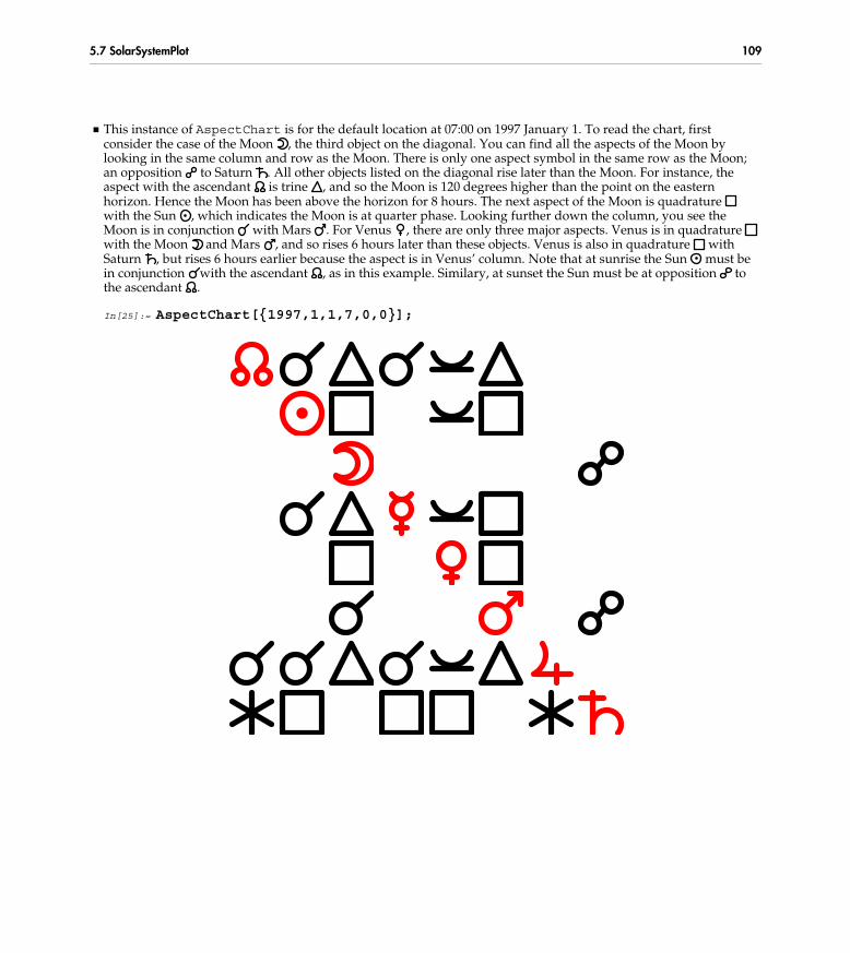
� This instance of AspectChart is for the default location at 07:00 on 1997 January 1. To read the chart, first consider the case of the Moon , the third object on the diagonal. You can find all the aspects of the Moon by looking in the same column and row as the Moon. There is only one aspect symbol in the same row as the Moon; an opposition to Saturn . All other objects listed on the diagonal rise later than the Moon. For instance, the aspect with the ascendant is trine , and so the Moon is 120 degrees higher than the point on the eastern horizon. Hence the Moon has been above the horizon for 8 hours. The next aspect of the Moon is quadrature with the Sun , which indicates the Moon is at quarter phase. Looking further down the column, you see the Moon is in conjunction with Mars . For Venus , there are only three major aspects. Venus is in quadrature with the Moon and Mars , and so rises 6 hours later than these objects. Venus is also in quadrature with Saturn , but rises 6 hours earlier because the aspect is in Venus’ column. Note that at sunrise the Sun must be in conjunction with the ascendant , as in this example. Similary, at sunset the Sun must be at opposition to the ascendant .
In[25]:= AspectChart[{1997,1,1,7,0,0}];
5.7 SolarSystemPlot 109

� The information returned by AspectChart is also contained in SolarSystemPlot. In this graphic you see all the aspects between the planets, Sun, and Moon. For instance, the conjunction of the Moon and Mars and the opposition of the Moon and Saturn are visible. Remember that the Earth is in the center of this graphic.
In[26]:= SolarSystemPlot[{1997,1,1,7,0,0}];
0h
Psc
2h
Ari
4hTau
6hGem8h
Cnc
10hLeo
12h
Vir
14h
Lib
16hSco 18h Sgr
20h
Cap
22h
Aqr
Morning
Evening
1997 �Jan�01
Some key points to be aware of are that the rising of any planet occurs when the planet is in conjunctionwith the ascendant. Similarly, a planet sets when it is in opposition to the ascendant. A full moon is inopposition to the Sun, and a new moon is in conjunction with the Sun. Venus is at its brightest when it isnot in conjunction with the Sun. Any object in quadrature with the ascendant is at its highest point inthe sky. These rules apply to other combinations of planets and aspects as well. Remember that theobject in the same row as an aspect rises before the object in the same column as the aspect.
When there are many alignments between the planets, AspectChart will indicate this with manyconjunction symbols.
110 5. Planet Plotting Functions

� At sunrise on 2000 May 4, the Sun, the Moon, and all the bright planets will rise as one above the eastern horizon. Although this type of cosmic alignment is relatively rare, it has happened before during the previous millenia (a similar event occurred at sunrise on 748 November 1). Here is an aspect chart clearly showing the alignment, with almost all objects in conjunction with the others. Mars is slightly out of the alignment, rising an hour too early.
In[27]:= AspectChart[SunRise[{2000,5,4}]];
The BirthChart Function
BirthChart produces a chart containing essentially the same information as SolarSystemPlot,except that it uses astrological symbols to represent the planets and the zodiac constellations. Thehorizontal line in the chart demarcates the regions above and below the horizon of an observer at thecenter of the chart. Thus, any planet symbol above this line corresponds to a planet above the observer'shorizon.
5.7 SolarSystemPlot 111

BirthChart�date� return the astrological birth chart for the given date
GeoLongitude �� longitude the geographic longitude to use for the chart
GeoLatitude �� latitude the geographic latitude to use for the chart
TimeZone �� timezone the time zone to use for the chart
Epoch �� Automatic the epoch to use for the position of the zodiac constellations;default is –�500.0 �corresponding to the year 500 B . C .�
Generating a birth chart.
The chart shows a circle containing the 12 zodiac signs with the position of the Sun, Moon, and mainplanets indicated relative to those signs. At the center of the chart is the Earth , and on the eastern andwestern horizons are the ascendant and descendant . Astrologers use the zodiac constellationnearest the Sun , at the time of birth, as the astrological sign of a person. The position of each zodiacconstellation is taken as it appeared in the year 500 B.C., however. Precession, as of the year 2000 A.D.,has moved the position of all the zodiac constellations more than one zodiac sign away, but this is notnormally taken into account by astrologers. In BirthChart you can use the option Epoch ->Automatic to get the true position of the zodiac constellations at the time of birth. The default isEpoch -> -500.0, which corresponds to the position of the zodiac constellations in the year 500 B.C.
112 5. Planet Plotting Functions

� This is the birth chart for the given date, with the specified geographic location and time zone. All the main planets are below the horizon.
In[28]:= BirthChart[{1993,11,17,3,20,0}, GeoLongitude -> 145.0*Degree,
GeoLatitude -> -37.8*Degree, TimeZone -> 11];
Astrological symbols used for the zodiac constellations are Aries , Taurus , Gemini , Cancer ,Leo , Virgo , Libra , Scorpius , Sagittarius , Capricornus , Aquarius , and Pisces .
The arrow in the chart corresponds to the direction of the meridian. For northern hemisphere observersthe meridian is due south, and for southern hemisphere observers it is due north. The meridian arrow isalways near the vertical in the chart, but it can vary up to 23 degrees on either side of the vertical due tothe tilt of the Earth's axis.
5.7 SolarSystemPlot 113

� This BirthChart is for the default location at 07:00 on 1997 January 1. It shows the Sun , Jupiter , and Mercury rising (or ascending) above the eastern horizon. This chart is for the southern hemisphere, so the ascendant is on the right, which is the opposite of its location on a northern hemisphere chart. Venus is higher in the sky near the zodiac sign of Sagittarius . The Moon and Mars are in conjunction near Virgo .
In[29]:= BirthChart[{1997,1,1,7,0,0}];
114 5. Planet Plotting Functions

� This is the birth chart for Charles Dickens, born at midnight on 1812 February 7. It shows all the planets below the horizon, with the exception of Jupiter . The position of the Sun is in Aquarius .
In[30]:= BirthChart[{1812,2,7,0,0,0}, GeoLongitude -> 0*Degree, GeoLatitude -> 51*Degree, TimeZone -> 0];
� 5.8 The JupiterSystemPlot Function
JupiterSystemPlot is useful for displaying a plot of the four Galilean moons orbiting Jupiter on agiven date.
JupiterSystemPlot�date� plot the general layout of the Galilean moons aroundJupiter on the given date
Plotting a representation of the Jovian moon system.
As seen from the Earth, the Galilean moons around Jupiter can undergo various special events everyfew days. Four types of events are possible. First, a moon can transit across the Jovian disk; second, a
5.8 JupiterSystemPlot 115

moon can cast a shadow on the Jovian disk; third, a moon can hide (or be occluded) behind the Joviandisk; and fourth, a moon can be eclipsed in the shadow of the Jovian disk.
All of these special events are indicated in the JupiterSystemPlot graphic for a given date and time.
� The moons Io and Ganymede both fall in the “Shadow” colored region in this graphic, which means their shadows are cast onto the Jovian disk. Similarly, Io falls in the “Transit” region, which means it is in front of the Jovian disk as seen from the Earth. You can confirm this with a call to PlanetPlot3D.
In[31]:= JupiterSystemPlot[{1993,11,17,21,20,0}];
Eclipse
Shadow
Occlude
Transit
IoEuropa
Ganymede Callisto
1993 �Nov�17 21:20:00East West
116 5. Planet Plotting Functions

� As expected, Ganymede’s shadow is ingressing on the left or eastern edge, and Io’s shadow is egressing on the right or western edge. The green dot is Io itself, which is making a transit.
In[32]:= PlanetPlot3D[Jupiter, {1993,11,17,21,20,0}];
� 5.9 The JupiterMoonChart Function
JupiterMoonChart produces a plot, for a specified period of time, of the positions of the four Galileanmoons orbiting Jupiter.
JupiterMoonChart�date1, date2�
chart the positions of the four Galilean moons as seenfrom Earth between the dates date1 and date2
JupiterMoonChart�date� produce a chart appropriate for the next four days after date
Charting Jovian moon positions.
In the graphic that is returned, the four Galilean moons Io, Europa, Ganymede, and Callisto are coloredblack, red, green, and blue respectively. Jupiter is colored purple, with the width of the linecorresponding to one Jovian diameter. The white line above the purple Jovian disk indicates when theGreat Red Spot is visible. It is visible for half of its roughly 10-hour rotation period. (You can adjust theposition of the spot by setting $JupiterGreatRedSpotLongitude .)
The horizontal scale is in Jovian radii, and the vertical axis shows time marked off in 6-hour intervals oflocal time, along with the day of the month.
5.9 JupiterMoonChart 117

� A JupiterMoonChart graphic displays a Jupiter moon finder chart beginning 1993 November 17 and ending four days later. Local night is shaded with gray bands.
Callisto, in blue and on the right in the graphic, starts off at about 15 Jovian radii west of Jupiter. Over the next couple of nights it moves further away to more than 26 Jovian radii before moving across to the eastern side of Jupiter.
Similary, Io, in black, is first hidden behind Jupiter and then moves to the east; by about 22:00 local time on November 17 it crosses back in front of Jupiter.
In[33]:= JupiterMoonChart[{1993,11,17}];
0
6
12
18
0
6
12
18
0
6
12
18
0
6
12
18
0
17
18
19
20
25 20 15 10 5 0 -5 -10 -15 -20 -25
��East � West��
1993 �Nov�17
Use the option Text->False to prevent the date being printed at the bottom of the chart.
118 5. Planet Plotting Functions

6. Eclipse Predicting FunctionsDuring a typical year the Moon orbits the Earth nearly 13 times. Two of those orbits usually pass soclose to the direction of the Sun that the Moon casts a shadow onto the surface of the Earth; such eventsare called solar eclipses. Depending on how close (from the Earth’s viewpoint) the Moon and the Sunare to each other, the event is termed either a partial, total, or annular solar eclipse.
You can compute and display such events using Scientific Astronomer. For instance, the package providesa function called Separation to compute the angular separation between any two celestial objects onany given date, as seen from any viewpoint. When the separation is zero, then one of the objects iseclipsed by the other. You can compute the precise date of such an event with a function likeSolarEclipse, and then use the PlanetPlot function to see how the shadow falls on the object.Additional functions, such as MoonShadow, are available to compute the precise position of the shadow;and EclipseBegin and EclipseEnd are used to give the precise start and end times of the eclipse asseen from a specific location.
Eclipses traditionally refer to alignments involving the Earth, the Moon, and the Sun. ScientificAstronomer, however, can handle alignments among any three objects. Typical cases are the Earth, theMoon, and a star for lunar occultations; the Sun or the Earth, with Jupiter and a Galilean moon forvarious types of shadows, transits, occultations, and eclipses; and the Sun, the Earth, and an inner planetfor transits of the planet across the solar disk.
Setting Your Time Zone
� Load the Scientific Astronomer package.
In[1]:= <<Astronomer`HomeSite`
Astronomer is Copyright �c� 1997 Stellar Software
This chapter does not include any function that requires a knowledge of your geographic location. Mostfunctions still require that you input your time zone, however; you can set this using SetLocation asnormal.
� This sets your time zone to 11 hours ahead of GMT.
In[2]:= SetLocation[TimeZone -> 11];
� 6.1 The EclipseTrackPlot Function
EclipseTrackPlot is useful for displaying details of the umbra and penumbra regions of either asolar or lunar eclipse. It can also be used to display tracks of occultations of stars or planets by the Moon.
6.1 EclipseTrackPlot 119

EclipseTrackPlot�object1, object2, object3, date�
plot the track of umbra � penumbra shadows of object2caused by the light from object3 as cast on the surface ofobject1 around the given date
EclipseTrackPlot�neardate� plot either the Earth or the Moon, depending on whetherneardate is near a new moon �for a solar eclipse� or a fullmoon �for a lunar eclipse�
Plotting the track of a solar or lunar eclipse.
In the graphic that is returned by EclipseTrackPlot, the gray area is the region that experiences apartial eclipse at some point during the eclipse. The upper and lower red lines represent the edges of thepartial eclipse shadow, and the green lines at the end represent the edges where the partial eclipseceases because of either sunrise or sunset.
� Here you see the track of the total solar eclipse of 1948 November 1.
In[3]:= EclipseTrackPlot[SolarEclipse[{1948,11,1}]];
A solar eclipse is only visible from a small portion of the Earth, perhaps a band 100km across, indicatedwith the black line.
Lunar Eclipses
A lunar eclipse is visible from half the Earth. You can view the eclipse from any point on the side of theEarth facing the Moon at the time it is occurring.
120 6. Eclipse Predicting Functions

� The lunar eclipse of June 1993 is total for 96 minutes and begins at 23:11 local time in Melbourne.
In[4]:= EclipseTrackPlot[LunarEclipse[{1993,6,5}]];
MoonPartial22:10Begin
Total23:11Begin
Total00:46End
Partial01:47End
WestEastPenumbra
Umbra
1993�Jun�04 23:58:33Partial for 217 min. Total for 96 min.
In the graphic, the Moon is the small circle in the center, and over time it sweeps across the band fromright to left. The two bigger disks represent the fixed umbra and penumbra shadows of the Earth.
Lunar Occultations
EclipseTrackPlot can also be used to find the regions on Earth in which you can see an occultationof a star or a planet by the Moon. A solar eclipse is also an occultation of the Sun by the Moon.
EclipseTrackPlot�Earth, Moon, Sun, date�
plot a solar eclipse track
EclipseTrackPlot�Earth, Moon, Spica, date�
plot a lunar occultation track of the star Spica
Plotting the track of a lunar occultation on the surface of the Earth.
6.1 EclipseTrackPlot 121

� On 1995 January 23, there is an occultation of the star Spica by the Moon, but it is visible only from North America. This is a track of the precise region from which the occultation is visible.
In[5]:= EclipseTrackPlot[Earth, Moon, Spica, {1995,1,23,11+11,0,0}];
As with PlanetPlot, you can use the option PlotRange to zoom into a smaller part of the surface ofthe Earth. The default is PlotRange -> {{-180, 180}, {-90, 90}}, which shows the entiresurface.
Note that you can use the function EclipseBegin to determine when the star Spica or any other star iseclipsed by the Moon.
� 6.2 The MoonShadow and SolarEclipse Functions
MoonShadow is useful for computing details of the Moon’s shadow during either a total or annular solareclipse. To determine the precise time of the solar eclipse, use SolarEclipse.
122 6. Eclipse Predicting Functions

MoonShadow�date� give the geographic location of the center of the Moon��sshadow, assuming it falls on the surface of the Earth onthe given date
SolarEclipse�neardate� compute the precise time of the next solar eclipse afterthe given neardate
SolarEclipse�� compute the time of the next solar eclipse
Separation �� separation the separation to use; default is 1.16 Degree, whichis large enough to catch both partial and total solar eclipses
Determing circumstances of solar eclipses.
A total solar eclipse is visible from only a small spot on the Earth, where it can last up to 7.6 minutes.You can use the option Separation to adjust how close the Sun and Moon have to be for the event tobe considered an eclipse. The default is Separation -> 1.16*Degree, which is large enough tocatch both partial and total solar eclipses. Reduce the separation if you are only interested in total solareclipses.
Note that the time returned by SolarEclipse is such that the separation of the Sun and the Moon is alocal minimum; that is, Separation[Sun, Moon, SolarEclipse[]] is a local minimum.
� This is the precise date and time of the middle of the annular solar eclipse in 1994.
In[6]:= SolarEclipse[{1994,1,1}]
Out[6]= �1994, 5, 11, 4, 11, 55�
� The location of the center of the shadow on the Earth’s surface at this time corresponds to a spot in North America. The degree of totality is only 0.89 at this particular time, so only 89% of the Sun is covered by the Moon; hence this is an annular eclipse. The annular eclipse lasts 6.0 minutes.
In[7]:= MoonShadow @ SolarEclipse[{1994,1,1}]
Out[7]= �GeoLongitude � �84.0582 Degree, GeoLatitude � 41.8139 Degree,Totality � 0.891507, Duration � �6.04025 Minute�
� The precise date and time of the middle of the total solar eclipse in 1994 is shown here.
In[8]:= SolarEclipse[{1994,6,1}]
Out[8]= �1994, 11, 4, 0, 38, 45�
6.2 MoonShadow and SolarEclipse 123

� In this example, the geographic location is off the coast of Argentina. The degree of totality is now 1.11, so 100% of the Sun is covered; hence this is a total eclipse. The total eclipse lasts 4.3 minutes.
In[9]:= MoonShadow @ SolarEclipse[{1994,6,1}]
Out[9]= �GeoLongitude � �35.9361 Degree, GeoLatitude � �35.8296 Degree,Totality � 1.10998, Duration � 4.32553 Minute�
� At the time of eclipse, and as viewed from the Moon’s shadow on the surface of the Earth, the Sun and Moon are separated by an extremely small angle.
In[10]:= Separation[Sun, Moon, SolarEclipse[{1994,6,1}], ViewPoint -> %]
Out[10]= 0.00012357 Degree
The third rule output from MoonShadow tells you how much of the area of the Sun is covered by theMoon as seen from Earth. The rule, therefore, represents the totality of the eclipse. If the totality isgreater than 1, the eclipse is total; if less than 1, the eclipse is annular.
The fourth rule tells you how long the Moon is in front of the Sun as seen from the returned geographiclocation given by the first two rules. This duration rule is the time interval between when the trailingedge of the Moon enters the solar disk and the leading edge of the Moon leaves the solar disk. Totaleclipses, therefore, have a positive duration, but annular eclipses, where the Sun is never fully covered,have a negative duration because the trailing edge of the Moon enters before the leading edge leaves.
The EarthShadow Function
A function related to MoonShadow is EarthShadow, which computes details of the Earth’s shadowduring a lunar eclipse. To determine the precise time of the lunar eclipse use LunarEclipse.
EarthShadow�date� give the position and size of the Earth��s shadow projectedat the distance of the Moon on the given date
LunarEclipse�neardate� compute the precise time of the next lunar eclipse afterthe given neardate
LunarEclipse�� compute the time of the next lunar eclipse
Separation �� separation the separation to use; default is 0.70 Degree, whichis large enough to catch both partial and total lunar eclipses
Determing circumstances of lunar eclipses.
A total lunar eclipse is visible from half the Earth (i.e., the side facing the Moon), where it can last up to 1hour 44 minutes. A partial lunar eclipse can last 4 hours. Use the option Separation to adjust howclose the Sun and Earth have to be, as seen from the Moon, for the event to be considered an eclipse. The
124 6. Eclipse Predicting Functions

default is Separation -> 0.70*Degree, which is large enough to catch both partial and total lunareclipses. Reduce the separation if you are only interested in total lunar eclipses.
Note that the time returned by LunarEclipse is such that the separation of the Sun and the Moon is alocal maximum near 180 degrees. That is, Separation[Sun, Moon, LunarEclipse[]] is a localmaximum.
� This is the precise time of the middle of a lunar eclipse in 1993.
In[11]:= LunarEclipse[{1993,11,17}]
Out[11]= �1993, 11, 29, 17, 27, 46�
� The Earth’s shadow is only 0.36 degrees away from the Moon at the middle of the lunar eclipse of 1993 November 29. The Moon itself is only half a degree in diameter, so this event is a total lunar eclipse.
In[12]:= Separation[Moon, EarthShadow[%], %]
Out[12]= 0.36338 Degree
� The shadow of the Earth during this lunar eclipse is a cone pointing in a direction specified by 4.3 hours of right ascension and 21.5 degrees of declination. The total shadow, at the distance of the Moon, is 1.3 degrees in diameter.
In[13]:= EarthShadow @ LunarEclipse[{1993,11,17}]
Out[13]= �Ascension � 4.34806 Hour, Declination � 21.4871 Degree,UmbraDiameter � 1.30801 Degree, PenumbraDiameter � 2.38874 Degree�
The output from EarthShadow contains information about the size of the umbra and penumbrashadows of the Earth projected at the distance of the Moon. The shadow of the Earth is a cone-shapedregion centered on the Sun and passing by the edges of the Earth. The third rule output fromEarthShadow gives the angular diameter of the umbra, or total shadow, of the Earth; the second rulegives the angular diameter of the penumbra, or partial shadow.
� 6.3 The EclipseBegin and EclipseEnd Functions
EclipseBegin and EclipseEnd are useful for determining the precise times when an object iseclipsed by a second object from the light from a third object. The diameters of the first and secondobjects are taken into account, but the third object is treated as a point source.
6.3 EclipseBegin and EclipseEnd 125

EclipseBegin�object1, object2, object3, neardate�
compute the precise date, nearest to neardate, at whichobject1 begins to be eclipsed by object2 from the light from object3
EclipseEnd�object1, object2, object3, neardate�compute the precise date, nearest to neardate, at whichobject1 ceases to be eclipsed by object2 from the light from object3
EclipseBegin�object, neardate� compute the precise date, nearest to neardate, at whichobject begins to be eclipsed by the Earth from the light ofthe Sun; this is equivalent toEclipseBegin�object,Earth, Sun, neardate�
EclipseEnd�object, neardate� compute the precise date, nearest to neardate, at which objectceases to be eclipsed by the Earth from the light of the Sun; thisis equivalent to EclipseEnd�object, Earth, Sun, neardate�
Beginning and ending times of an eclipse.
You can determine, for instance, when the Galilean moon Io is just beginning to be eclipsed from theSun by Jupiter moving between the two objects. Similarly, you can determine when the Great Red Spotis next visible.
� Io is eclipsed from the Sun at 16:46 on 1993 November 18.
In[14]:= EclipseBegin[Io, Jupiter, Sun, {1993,11,17,3,20,0}]
Out[14]= �1993, 11, 18, 16, 45, 54�
� A short time later, at 17:05, Io moves behind the Jovian disk, as seen from Earth.
In[15]:= EclipseBegin[Io, Jupiter, Earth, {1993,11,17,3,20,0}]
Out[15]= �1993, 11, 18, 17, 5, 10�
� Io reappears, in sunlight, on the other side of the Jovian disk about two hours later, at 19:17.
In[16]:= EclipseEnd[Io, Jupiter, Earth, {1993,11,17,3,20,0}]
Out[16]= �1993, 11, 18, 19, 17, 4�
� The Great Red Spot is next visible at 05:45 on 1993 November 17.
In[17]:= EclipseBegin[Jupiter, JupiterGreatRedSpot, Earth, {1993,11,17,3,20,0}]
Out[17]= �1993, 11, 17, 5, 45, 34�
126 6. Eclipse Predicting Functions

� It rotates out of view roughly 5 hours later at 10:43.
In[18]:= EclipseEnd[Jupiter, JupiterGreatRedSpot, Earth, {1993,11,17,3,20,0}]
Out[18]= �1993, 11, 17, 10, 43, 28�
Other Uses
Since three objects are normally supplied to EclipseBegin and EclipseEnd, you can search formany different types of events. Use them for solar and lunar eclipses; satellites disappearing into Earth’sshadow; transits of Mercury or Venus across the solar disk; transits, shadows, occultations, and eclipsesof the Galilean moons; and lunar occultations of stars by the Moon.
EclipseBegin�Sun, Moon, TopoCentric�
compute the time when a solar eclipse is overhead
EclipseBegin�Earth, Moon, Sun�
compute the time of the next solar eclipse somewhere on Earth
EclipseBegin�Moon, Earth, Sun�
compute the time of the next lunar eclipse
Beginning time of a solar or lunar eclipse.
EclipseBegin�Sun, Mercury, Earth�
compute the time when Mercury transits across the solar disk
EclipseBegin�Sun, Venus, Earth�
compute the time when Venus transits across the solar disk
Beginning time of a transit of Mercury or Venus.
EclipseBegin�Jupiter, Io, Earth�
compute the time when Io transits across the Jovian disk
EclipseBegin�Jupiter, Io, Sun�
compute the time when Io��s shadow is cast on the Jovian disk
EclipseBegin�Io, Jupiter, Earth�
compute the time when Io is occulted by the Jovian disk
EclipseBegin�Io, Jupiter, Sun�
compute the time when Io is eclipsed from the Sun bythe Jovian disk
Beginning time of various Jovian moon events.
6.3 EclipseBegin and EclipseEnd 127

EclipseBegin�Jupiter, JupiterGreatRedSpot, Earth�
compute the time when the Great Red Spot is visible
Beginning time of Great Red Spot visibility.
EclipseBegin�Earth, Moon, Spica�
compute the time of a lunar occultation of the star Spica
EclipseBegin�Spica, Moon, TopoCentric�
compute the time of the next lunar occultation overhead
Beginning time of a lunar occultation.
EclipseBegin�Mir, Earth, Sun�
compute the time when a satellite disappears into the Earth��sshadow
Beginning time of satellite disappearance.
Although the order of the objects might appear confusing, there is a consistency to it. Remember that thelast object is the one treated as a point source, whereas the first two objects are treated as disks of thecorrect size.
Thus EclipseBegin[Earth, Moon, Sun] determines when any part of the Moon’s disk begins tomove in front of any part of the disk of the Earth, as viewed from the center of the Sun. This is the timewhen a partial solar eclipse becomes visible from somewhere on Earth.
Similarly, EclipseBegin[Sun, Moon, TopoCentric] determines when any part of the Moon’sdisk begins to move between any part of the disk of the Sun and the current location on Earth. This isthe time when a solar eclipse becomes visible from the current topocentric location.
� A near total solar eclipse occurred over the lower part of the Pacific in February, 1981.
In[19]:= eclipse1981 = SolarEclipse[{1981,2,5}]
Out[19]= �1981, 2, 5, 9, 10, 22�
� The eclipse nearly passed over Melbourne, Australia. Here the site location of Melbourne is set.
In[20]:= SetLocation[GeoLongitude -> 145.0*Degree, GeoLatitude -> -37.8*Degree, GeoAltitude -> 0.0*KiloMeter, TimeZone -> 11];
128 6. Eclipse Predicting Functions

� The partial eclipse phase begins at 06:33 for observers located at Melbourne, Australia. (TopoCentric represents the location set earlier with SetLocation.)
In[21]:= EclipseBegin[Sun, Moon, TopoCentric, eclipse1981]
Out[21]= �1981, 2, 5, 6, 33, 11�
� The partial eclipse phase ends at 08:34 for observers located at Melbourne, Australia.
In[22]:= EclipseEnd[Sun, Moon, TopoCentric, eclipse1981]
Out[22]= �1981, 2, 5, 8, 34, 23�
� The average of the two times above is the approximate time of maximum eclipse for the location. By trial and error minimizing Separation[Sun, Moon, date, ViewPoint->TopoCentric] you find the actual time of maximum eclipse occurs about three minutes earlier.
In[23]:= besttime = {1981,2,5,7,30,59}
Out[23]= �1981, 2, 5, 7, 30, 59�
� The maximum eclipse happens only an hour after sunrise for observers located at Melbourne.
In[24]:= SunRise[eclipse1981]
Out[24]= �1981, 2, 5, 6, 39, 32�
� The eclipse appears 9 degrees above the eastern horizon.
In[25]:= HorizonCoordinates[Moon, besttime, ViewPoint -> TopoCentric]
Out[25]= �Azimuth � 103.305 Degree, Altitude � 9.21132 Degree,Distance � 375203. KiloMeter�
6.3 EclipseBegin and EclipseEnd 129

� This is how the eclipse appeared at its maximum.
In[26]:= PlanetPlot3D[Sun, besttime, ViewPoint -> TopoCentric, ViewVertical -> Zenith];
Jovian Moon Events
As mentioned earlier, EclipseBegin and EclipseEnd can be used to determine the precise time ofvarious alignments involving the Earth, the Sun, Jupiter, and a Galilean moon. There are essentially fourtypes of events that can take place.
A Jovian eclipse occurs when a moon of Jupiter is blocked from the light of the Sun; this is an alignmentinvolving the Jovian moon, Jupiter, and the Sun. A Jovian occultation occurs when a moon of Jupiter ishidden behind the Jovian disk as seen from the Earth; this is an alignment involving the Jovian moon,Jupiter, and the Earth. A Jovian shadow occurs when the shadow of a moon of Jupiter passes across theJovian disk; this is an alignment involving Jupiter, the Jovian moon, and the Sun. A Jovian transit occurswhen a moon of Jupiter passes across the Jovian disk as seen from the Earth; this is an alignmentinvolving Jupiter, the Jovian moon, and the Earth.
� Here are two functions which compute the disappearance and reappearance times of a Jovian eclipse (i.e., a Jovian moon blocked from the light of the Sun).
In[27]:= EclipseDisappear[jovianMoon_, neardate___] := EclipseBegin[jovianMoon, Jupiter, Sun, neardate]
In[28]:= EclipseReappear[jovianMoon_, neardate___] := EclipseEnd[jovianMoon, Jupiter, Sun, neardate]
130 6. Eclipse Predicting Functions

� Here are two functions which compute the disappearance and reappearance times of a Jovian occultation (i.e., a Jovian moon hidden behind the Jovian disk).
In[29]:= OccludeDisappear[jovianMoon_, neardate___] := EclipseBegin[jovianMoon, Jupiter, Earth, neardate]
In[30]:= OccludeReappear[jovianMoon_, neardate___] := EclipseEnd[jovianMoon, Jupiter, Earth, neardate]
� Here are two functions which compute the ingress and egress times of a Jovian moon’s shadow across the Jovian disk.
In[31]:= ShadowIngress[jovianMoon_, neardate___] := EclipseBegin[Jupiter, jovianMoon, Sun, neardate]
In[32]:= ShadowEgress[jovianMoon_, neardate___] := EclipseEnd[Jupiter, jovianMoon, Sun, neardate]
� Here are two functions which compute the ingress and egress times of a transit of a Jovian moon across the Jovian disk.
In[33]:= TransitIngress[jovianMoon_, neardate___] := EclipseBegin[Jupiter, jovianMoon, Earth, neardate]
In[34]:= TransitEgress[jovianMoon_, neardate___] := EclipseEnd[Jupiter, jovianMoon, Earth, neardate]
� 6.4 The EclipseQ Function
EclipseQ is useful for deciding when an object is eclipsed by a second object from the light of a thirdobject. The diameters of the first and second objects are taken into account, but the third object is treatedas a point source.
EclipseQ�object1, object2, object3, date�
test if object1 is eclipsed by object2 from the light of object3on the given date
EclipseQ�object, date� test if object is eclipsed by the Earth from thelight of the Sun on the given date; this is equivalent toEclipseQ�object, Earth, Sun, date�
Testing for eclipses.
The EclipseQ function returns either True or False to questions you input concerning eclipse events.EclipseQ will sometimes tell you something you already know. You can, for example, confirm that theMoon is really eclipsed by the Earth from the Sun during a lunar eclipse. Similarly, you can confirm thatthe Earth is really eclipsed by the Moon from the Sun during a solar eclipse.
6.4 EclipseQ 131

� By definition, the Moon is eclipsed during a lunar eclipse.
In[35]:= EclipseQ[Moon, LunarEclipse[]]
Out[35]= True
� Part of the Earth is eclipsed by the Moon from the Sun during a solar eclipse.
In[36]:= EclipseQ[Earth, Moon, Sun, SolarEclipse[]]
Out[36]= True
Other uses of EclipseQ are possible. For instance, a transit of Venus occurred in the year 1769; todetermine its precise time you can experiment with different date arguments.
� The transit of Venus has not started at this time.
In[37]:= EclipseQ[Sun, Venus, Earth, {1769,6,4,6,0,0}]
Out[37]= False
� Now Venus is in transit.
In[38]:= EclipseQ[Sun, Venus, Earth, {1769,6,4,9,0,0}]
Out[38]= True
� Now it has finished its transit.
In[39]:= EclipseQ[Sun, Venus, Earth, {1769,6,4,13,0,0}]
Out[39]= False
Of course, the precise beginning and ending of the transit can more easily be determined withEclipseBegin and EclipseEnd.
� The transit begins at 06:16 Melbourne time on 1769 June 4.
In[40]:= EclipseBegin[Sun, Venus, Earth, {1762,1,1}]
Out[40]= �1769, 6, 4, 6, 15, 41�
� It ends 6 hours later at 12:34.
In[41]:= EclipseEnd[Sun, Venus, Earth, {1762,1,1}]
Out[41]= �1769, 6, 4, 12, 34, 3�
132 6. Eclipse Predicting Functions

Additionally, EclipseQ will test for conjunctions or lunar occultations. You can also determine whenthe Galilean moons Io, Europa, Ganymede, and Callisto undergo, say, a transit or occultation from theEarth, or an eclipse or shadow from the Sun.
� This confirms the rare Mars-Venus conjunction in the year 1590.
In[42]:= EclipseQ[Mars, Venus, Earth, {1590,10,13,15,58,0}]
Out[42]= True
� This verifies the lunar occultation of the star Spica in 1995. The Moon passed directly between the Earth and Spica on 1995 January 23 at 22:00.
In[43]:= EclipseQ[Earth, Moon, Spica, {1995,1,23,22,0,0}]
Out[43]= True
� On the given date, Io is not in transit across the Jovian disk.
In[44]:= EclipseQ[Jupiter, Io, Earth, {1993,11,17,3,20,0}]
Out[44]= False
� 6.5 The Conjunction and ConjunctionEvents Functions
When two objects move close together in the sky, they are said to be in conjunction. The Conjunctionfunction is useful for determining the approximate date of such an event.
Conjunctions are usually of little astronomical importance, but they do make interesting events forcasual observers to witness. A grazing occultation, however, can give detailed information about theshape and atmosphere of the occluding object.
Conjunction�object1, object2, neardate�
find the date, nearest to neardate, at which the rightascension of object1 will align with the right ascension of object2
Conjunction�object1, object2� find the conjunction date nearest the current value of Date��
Determing the time of a conjunction.
You can use Conjunction to find the approximate date when Jupiter and Mars align nearest a givendate. The correct date for the nearest conjunction to 1995 January 1 is 1995 November 17, and you candetermine this date precisely using Separation.
6.5 Conjunction and ConjunctionEvents 133

� Jupiter and Mars align 10 months after the given date on about 1995 November 17.
In[45]:= Conjunction[Jupiter, Mars, {1995,1,1}]
Out[45]= �1995, 11, 17�
� On 1995 November 17, Jupiter and Mars are just 1.2 degrees apart in the sky.
In[46]:= Separation[Jupiter, Mars, {1995,11,17}]
Out[46]= 1.20348 Degree
Precise Conjunctions
A very precise conjunction between Venus and Mars took place in the year 1590. At the time of theconjunction, the angular radius of Venus is bigger than the Mars-Venus separation, so you can concludethat Venus totally occluded Mars on 1590 October 13. This was a very rare event.
� During 1590, Mars and Venus align on about October 14.
In[47]:= Conjunction[Mars, Venus, {1590,8,1}]
Out[47]= �1590, 10, 14�
� The precise time of the conjunction is October 13, at 15:58, at which point the separation is just 0.0016 degrees.
In[48]:= Separation[Mars, Venus, {1590,10,13,15,58,0}]
Out[48]= 0.00164543 Degree
� The angular radius of Venus is 0.0018 degrees, which is greater than the separation.
In[49]:= ApparentDiameter/2 /. Appearance[Venus, {1590,10,13,15,58,0}]
Out[49]= 0.00181081 Degree
The ConjunctionEvents Function
A related function is ConjunctionEvents, which finds all the conjunctions between major solarsystem objects during a given month. It returns a list of days in the month showing the objects that align,and how close they are to each other.
134 6. Eclipse Predicting Functions

ConjunctionEvents�neardate� list all the conjunctions between the major planets, asteroids,ecliptic stars, and the Moon, during the month nearest neardate
ConjunctionEvents�� list the conjunctions for the current month
Searching for conjunction events.
Most objects in the solar system move near the ecliptic line, so chance alignments between pairs ofobjects are relatively common. A close conjunction between Venus and a new moon is a sight worthseeing.
� This shows all the conjunctions between the major solar system objects during November, 1993. It shows, for instance, that Jupiter is 0.4 degrees north of Venus on November 9. The Moon and the Sun are 0.2 degrees apart on November 15, so there is a solar eclipse visible at some location on the Earth on this date.
In[50]:= ConjunctionEvents[{1993,11,17}]
Conjunctions during November, 1993 areNov 3: Aldebaran 4.5° south of MoonNov 5: Spica 3.5° south of VenusNov 9: Jupiter 0.4° south of VenusNov 9: Regulus 5.7° north of MoonNov 13: Jupiter 3.9° north of MoonNov 13: Mercury 1.7° north of SunNov 13: Spica 0.7° north of MoonNov 14: Venus 2.9° north of MoonNov 15: Mercury 2.2° north of MoonNov 15: Moon 0.2° south of SunNov 16: Mars 1.6° south of MoonNov 16: Antares 5.7° south of MoonNov 19: Uranus 4.7° south of MoonNov 22: Saturn 6.8° south of MoonNov 23: Vesta 12.9° south of MoonNov 23: Antares 4.1° south of MarsNov 26: Mercury 1.2° north of VenusNov 29: Pleiades 3.6° north of Moon
Out[50]= �ConjunctionData�
6.5 Conjunction and ConjunctionEvents 135


7. Satellite Tracking FunctionsMany low-orbit Earth satellites are visible to the naked eye, but to spot them requires a knowledge ofexactly when to look. The window of opportunity is about two minutes wide and occurs at a time justafter dusk or just before dawn.
The Mir Space Station is the best and brightest object to see. It can appear as bright as the brightest stars.A Space Shuttle can also appear as bright as Mir, but missions are relatively infequent.
Other satellites that sometimes appear bright are the Hubble Space Telescope (HST), the UpperAtmosphere Research Satellite (UARS), and the Cosmic Background Explorer (COBE).
Scientific Astronomer provides several functions for adding and analyzing the orbit of satellites. Thesefunctions are able to add comets and extra asteroids as well as objects in orbit around other planets ormoons.
� Load the package.
In[1]:= <<Astronomer`HomeSite`
Astronomer is Copyright �c� 1997 Stellar Software
� This sets your location and time zone.
In[2]:= SetLocation[GeoLongitude -> 145.0*Degree, GeoLatitude -> -37.8*Degree, GeoAltitude -> 0.0*KiloMeter, TimeZone -> 11];
� 7.1 The SetOrbitalElements Function
SetOrbitalElements lets you add a new object. Many objects, such as planets and asteroids, arealready built into Scientific Astronomer, but occasionally you may need to add other objects such as low-orbit Earth satellites or comets.
Most objects are in orbit around a parent body. To add such an object to Scientific Astronomer, you needto know the orbital elements of the object.
7.1 SetOrbitalElements 137

SetOrbitalElements�newobject, elements...�define a new object with the given orbital elements
Date �� date elements for the given date
ViewPoint �� parentbody orbit centered on parentbody
OrbitalSemiMajorAxis �� lengththe semimajor axis length of the orbit
OrbitalEccentricity �� eccentricitythe eccentricity of the orbit
OrbitalInclination �� inclinationthe inclination of the orbit to the equator
OrbitalPeriod �� period the period of the orbit in days
MeanAnomaly �� anomaly the mean anomaly of the orbit
PerigeeArgument �� perigee the perigee argument of the orbit
AscendingLongitude �� ascensionthe longitude of the ascending node of the orbit
Setting the elements of a new object.
Orbital elements are a set of numbers that describe the shape, and other details, of an object’s orbit. Theelements are represented by the quantities OrbitalSemiMajorAxis, OrbitalEccentricity,OrbitalInclination, MeanAnomaly, PerigeeArgument, AscendingLongitude,OrbitalMeanMotion, and OrbitalDecayRate. You may choose to specify OrbitalPerigee ratherthan OrbitalSemiMajorAxis, and PerigeeDate rather than MeanAnomaly. Similarly, you maychoose to specify OrbitalPeriod rather than OrbitalMeanMotion. Conversion formulae arediscussed at the end of this section.
You can use SetOrbitalElements to add comets, such as Halley or Hale-Bopp, or other objects suchas asteroids. You can even use it to add satellites in orbit about the Earth.
Often, however, you only know the NORAD two-line elements of a low-orbit satellite, rather than theproper orbital elements. Two-line elements for thousands of satellites are available and regularlyupdated on the Internet. You can use a function called TwoLineElements to convert the NORAD two-line elements into a form suitable for use with SetOrbitalElements.
SetOrbitalElements�newobject, line1, line2�
define a new object with the given NORAD two-lineorbital elements line1 and line2
TwoLineElements�line1, line2� convert from standard NORAD two-line orbital element setformat, to rules suitable for use with SetOrbitalElements
Converting NORAD elements.
138 7. Satellite Tracking Functions

� Convert the two-line elements of the Mir Space Station into a form suitable for use with SetOrbitalElements.
In[3]:= TwoLineElements[ "1 16609U 86017A 95025.53583445 .00005100 00000-0 71581-4 0 9062", "2 16609 51.6458 152.6933 0001412 164.2374 195.8663 15.58639897510653"]
Out[3]= �ViewPoint � Earth, Date � 34723.5, OrbitalMeanMotion �
15.58639897 Revs���������������������������������������������������
Day, OrbitalDecayRate �
0.000051 Revs������������������������������������������
Day2,
OrbitalSemiMajorAxis � 6792.12 KiloMeter,OrbitalEccentricity � 0.0001412, OrbitalInclination � 51.6458 Degree,MeanAnomaly � 195.8663 Degree, PerigeeArgument � 164.2374 Degree,
AscendingLongitude � 152.6933 Degree�
� Here the two-line elements are directly used to set the elements of Mir.
In[4]:= SetOrbitalElements[Mir, "1 16609U 86017A 95025.53583445 .00005100 00000-0 71581-4 0 9062", "2 16609 51.6458 152.6933 0001412 164.2374 195.8663 15.58639897510653"];
� These are the orbital elements of the STS-58 Space Shuttle mission.
In[5]:= SetOrbitalElements[STS58, ViewPoint -> Earth, Date -> {1993, 1, 280.67747791, TimeZone /. GetLocation[], 0, 0}, OrbitalMeanMotion -> 15.96123499*Revs/Day, OrbitalDecayRate -> 0.00119475*Revs/Day^2, OrbitalSemiMajorAxis -> 6684.521 * KiloMeter, OrbitalEccentricity -> 0.0007676, OrbitalInclination -> 39.0114*Degree, MeanAnomaly -> 89.5676*Degree, PerigeeArgument -> 272.4217*Degree, AscendingLongitude -> 117.7673*Degree];
SetOrbitalElements allows you to add virtually any type of new object orbiting any other object.Use the function SetCoordinates if you do not want the object to gravitationally orbit another object.This function lets you define the x,y,z coordinates of the object as a function of time.
Remember that the two-line elements of any low-orbit satellite are accurate for only a few monthsaround the epoch date, beyond which considerable error may result in an orbit calculation. The epochdate for the Mir element set used in the example earlier is the 25.5th day of 1995, so by the end ofFebruary 1995, you would not use the element set if you required high accuracy.
7.1 SetOrbitalElements 139

Element dates are usually expressed in Universal Time (UT). Scientific Astronomer, however, uses localtime for all dates. Therefore, if you enter an element date via the Date option toSetOrbitalElements, you must add a time zone correction.
The element date for the STS-58 Space Shuttle example above is the instant 280.67747791 days after thebeginning of 1993 in UT. Thus, the element date is entered as Date -> {1993, 1, 280.67747791,TimeZone /. GetLocation[], 0, 0}, which includes the time zone correction for your location.
An alternative is to supply the option TimeZone -> 0 to SetOrbitalElements, which temporarilyswitches to UT (or time zone 0). In this case, you can enter the element date as Date ->{1993,1,280.67747791}.
Tracking a Satellite
Once a new object like Mir has been added, you can begin to use it in other functions. In particular, youcan use the object in OrbitTrack to superimpose a track of the Mir Space Station onto a star chart, if itmakes a transit directly over your location.
At some point along the track, Mir disappears as it moves into the Earth’s shadow. It takes less than fiveseconds to fade, and you can compute the precise time of the disappearance using EclipseBeginapplied to the object Mir. The precise altitude, or angle above the horizon, of the disappearance isdetermined using HorizonCoordinates.
� Compute a best visibility date of Mir.
In[6]:= BestView[Mir, {1995,1,31}]
Out[6]= �TransitVisible � �1995, 2, 1, 21, 48, 59��
140 7. Satellite Tracking Functions

� During transit visibility, Mir takes about 10 minutes to cross from the southwest horizon to the northeast horizon. To show the track in the southern part of the sky use CompassStarChart with an Epilog option containing an OrbitTrack function.
In[7]:= CompassStarChart[South, {1995,2,1,21,50,0}, Mesh -> True, MagnitudeRange -> 4.0, Ecliptic -> False, Epilog -> { RGBColor[1,0,0], OrbitTrack[Mir, {1995,2,1,21,49-6,0}, {1995,2,1,21,49+6,0}, ViewPoint -> TopoCentric, PlotPoints -> 200], RGBColor[0,0,0], Table[Text[m, ChartCoordinates[Mir, {1995,2,1,21,m,0}, ViewPoint -> TopoCentric]], {m, 49-6, 49+6, 1}]}];
43444546
47
48
49
East South West
Feb 01
21:50
Latitude
38 South
� This shows that Mir disappears at 9:50:46 local time. Before this disappearance time there are several minutes of visibility.
In[8]:= EclipseBegin[Mir, {1995,2,1,21,49,0}]
Out[8]= �1995, 2, 1, 21, 50, 46�
7.1 SetOrbitalElements 141

� Mir disappears at about 29 degrees up in the east-northeast sky.
In[9]:= HorizonCoordinates[Mir, {1995,2,1,21,50,46}, ViewPoint -> TopoCentric]
Out[9]= �Azimuth � 60.8869 Degree, Altitude � 28.7719 Degree,Distance � 801.665 KiloMeter�
Do not forget to use the option setting ViewPoint -> TopoCentric in a function likeHorizonCoordinates, when dealing with a low-orbit satellite. This applies to functions likeOrbitTrack, Ephemeris, HorizonCoordinates, EquatorCoordinates, ChartCoordinates,Separation, Elongation, and Conjunction. The default for those functions is ViewPoint ->Earth, so you must specify ViewPoint -> TopoCentric as it is important to measure angles fromthe surface of the Earth, rather than the center, when dealing with satellites.
Adding a Comet
Although SetOrbitalElements is mainly used to add Earth satellites, such as the Mir Space Stationor a Space Shuttle mission, you can use it to add other objects. For instance, if you know the orbitalelements you can add Comet Halley.
� This adds the new object named Halley.
In[10]:= SetOrbitalElements[Halley, ViewPoint -> Sun, Date -> {1986, 2, 9.4589, TimeZone /. GetLocation[], 0, 0}, OrbitalSemiMajorAxis -> 17.9416 * AU, OrbitalEccentricity -> 0.967277, OrbitalInclination -> 162.2422*Degree, MeanAnomaly -> 0 *Degree, PerigeeArgument -> 111.8657*Degree, AscendingLongitude -> 58.8601*Degree];
Once Halley has been added, you can begin to use it in other functions. For example, you can projectits motion onto a star chart just like Mir.
Sometimes the published orbital elements of an object, such as a comet, use the perigee distance ratherthan the semimajor axis distance. To convert, simply use the relation OrbitalSemiMajorAxis =OrbitalPerigee / (1 - OrbitalEccentricity), where OrbitalPerigee is the published perigee distance inastronomical units. Similarly, the perigee date, rather than the mean anomaly, might be given. In thiscase use the relation MeanAnomaly = Mod[-(PerigeeDate - Date) / (OrbitalPeriod/Day), 1] *360*Degree. If the orbital period is not specified, use the relation OrbitalPeriod =�OrbitalSemiMajorAxis �AU�
3�2*365.25*Day, which is applicable if the object is orbiting the Sun. Ofcourse, if the mean motion is given, simply use OrbitalPeriod = Revs/OrbitalMeanMotion. For CometHalley the orbital period is approximately 27757.7*Day, which is nearly 76 years.
142 7. Satellite Tracking Functions

� 7.2 The GetLocation Function
GetLocation computes the location of an object in a coordinate system similar to that used bySetLocation.
GetLocation�object, date� return the geographic location of the object on the given date
GetLocation�� return the current geographic location,as set usingSetLocation
Computing an object’s position in geographic coordinates.
Consider, for example, the Mir Space Station. Once an object representing Mir has been added, you canuse BestView to determine the times when Mir is making a visible transit pass overhead. Then useGetLocation to determine the location of Mir at that transit visible time. The location returned will bevery close to the current site location, because Mir is traveling overhead. It is only visible for a minute orso on either side of the transit visible time; as mentioned earlier, the window for viewing a low-orbitsatellite is always very narrow.
� This adds the new object Mir, with elements appropriate for its orbit in late January 1995.
In[11]:= SetOrbitalElements[Mir, "1 16609U 86017A 95025.53583445 .00005100 00000-0 71581-4 0 9062", "2 16609 51.6458 152.6933 0001412 164.2374 195.8663 15.58639897510653"];
� The next transit visible pass after January 20 is on January 30.
In[12]:= BestView[Mir, {1995,1,20}]
Out[12]= �TransitVisible � �1995, 1, 30, 22, 5, 7��
� At 21:49 on 1995 February 1, it is possible to see Mir from the current location.
In[13]:= BestView[Mir, {1995,1,31}]
Out[13]= �TransitVisible � �1995, 2, 1, 21, 48, 59��
� This gives the geographic location of Mir during the transit visible pass overhead.
In[14]:= GetLocation[Mir, {1995,2,1,21,49,0}]
Out[14]= �GeoLongitude � 145.061 Degree, GeoLatitude � �39.0522 Degree,GeoAltitude � 422.66 KiloMeter�
7.2 GetLocation 143

� Mir is 70.4 degrees above the horizon, and thus very high in the sky, traveling overhead at the given time.
In[15]:= HorizonCoordinates[Mir, {1995,2,1,21,49,0}, ViewPoint -> TopoCentric]
Out[15]= �Azimuth � 177.925 Degree, Altitude � 70.3724 Degree,Distance � 446.491 KiloMeter�
If you are tracking a satellite with radio equipment, visibility is not so important since all you need toknow is approximately when the object is overhead. Culmination gives you the time when an object isnext highest in the sky, and you can apply Ephemeris to determine the circumstances of the pass.
� Culmination gives the time when Mir is next highest in the sky overhead.
In[16]:= Culmination[Mir, {1995,2,1,15,0,0}]
Out[16]= �1995, 2, 1, 15, 21, 21�
GetLocation can, of course, be applied to other objects and not simply low-orbit Earth satellites. Forexample, use GetLocation to determine the part of the Earth that has the Moon directly overhead atany given time.
� On the given date, the Moon is directly over the point with longitude -29 degrees and latitude -21 degrees, which is a location off the east coast of Brazil.
In[17]:= GetLocation[Moon, {1993,11,17,3,20,0}]
Out[17]= �GeoLongitude � �29.0329 Degree, GeoLatitude � �20.9029 Degree,GeoAltitude � 367126. KiloMeter�
� 7.3 The OrbitTrackPlot Function
OrbitTrackPlot is useful for displaying the track of a low-orbit satellite onto the surface of the Earth.
144 7. Satellite Tracking Functions

OrbitTrackPlot�object, date1, date2�
plot the track of the object as projected onto the Earth��ssurface between date1 and date2
OrbitTrackPlot��object1, object2, ...�, date1, date2�
display the tracks of several objects at once
LocationRing �� True a 15 degree green ring around your current location on Earth
Shading �� True shading of the night side of the Earth
FeatureLabels �� True labeling of features on the planet
Features �� features additional surface features
PlotPoints �� n the number of line segments; default is 25
PlotRange �� range a smaller section of the plot
PlotStyle �� styles individual graphic styles for the tracks
Plotting orbital tracks.
Locations along the track are such that the object is directly overhead at some time between the givendates. The object will normally be an Earth satellite, but it can be a planet or any other object. The redregions indicate where the object is located overhead just after dusk in the evening sky. Similarly, theblue regions indicate the object’s location overhead just before dawn in the morning sky.
If the object you are tracking is a low-orbit Earth satellite, then the red and blue regions represent thewindows of opportunity to view the satellite. These are time periods of perhaps 5 or 10 minutes, whilethe satellite is still illuminated by the Sun but your viewing location is in darkness.
A sequence of tracks is displayed if you supply a list of objects, rather than a single object, as the firstargument to OrbitTrackPlot. In this case, you can also use the option PlotStyle to set a differentstyle for each track.
� Enter the orbital elements of a Space Shuttle mission.
In[18]:= SetOrbitalElements[STS63, ViewPoint -> Earth, Date -> {1995,2,3,6+11,48,13}, OrbitalMeanMotion -> 15.82619484*Revs/Day, OrbitalDecayRate -> 0.00000387*Revs/Day^2, OrbitalSemiMajorAxis -> 6723.340*KiloMeter, OrbitalEccentricity -> 0.0026128, OrbitalInclination -> 51.6614*Degree, MeanAnomaly -> 156.9459*Degree, PerigeeArgument -> 202.9294*Degree, AscendingLongitude -> 109.1408*Degree];
7.3 OrbitTrackPlot 145

� This graphic shows the track of the Space Shuttle mission for 6 hours, or about 4 orbits. Various evening passes are visible over parts of Australia, in addition to some morning passes over parts of North America.
In[19]:= OrbitTrackPlot[STS63, {1995,2,6, 8+11,0,0}, {1995,2,6,14+11,0,0}, PlotPoints -> 250, LocationRing -> True];
The option setting LocationRing -> True draws a green ring around the current site location. If anytrack passes within that ring, then the object is above the local horizon. When this occurs the object maybe tracked with radio equipment.
If the start and stop dates used by OrbitTrackPlot are sufficiently close, it makes sense to use theoption setting Shading -> True. This option works just as it does in PlanetPlot, shading the night-time region.
Again, the option PlotRange is available if you need to zoom into a smaller region on the surface of theEarth. The default is PlotRange -> {{-180, 180}, {-90, 90}}.
146 7. Satellite Tracking Functions

� This shows that visibility occurs around dawn and dusk only.
In[20]:= OrbitTrackPlot[STS63, {1995,2,6,8+11,0,0}, {1995,2,6,9+11,0,0}, PlotPoints -> 50, Shading -> True];
� The option PlotRange is used here to zoom into the area over Australia.
In[21]:= OrbitTrackPlot[STS63, {1995,2,6,8+11,0,0}, {1995,2,6,9+11,0,0}, PlotPoints -> 50, Shading -> True, PlotRange -> {{90, 180}, {-50, 10}}];
7.3 OrbitTrackPlot 147

� 7.4 The OrbitPlot and OrbitPlot3D Functions
OrbitPlot plots the elliptical orbit of an object or objects about a common center.
OrbitPlot��object1, object2, ...��
plot the full elliptical orbit of all the objects about their commoncenter; you can specify a date if the orbit changes with time
OrbitPlot3D��object1, object2, ...��
make a three-dimensional plot of the full ellipticalorbit of all the objects about their common center;you can specify a date if the orbit changes with time
PlotStyle �� styles individual graphic styles for the orbits
Distance �� distance a bigger or smaller field of view; default is 12 AU
Plotting the shape of an orbit.
In the two-dimensional form, the horizontal axis is aligned so that the right points to the zero hour ofright ascension, and the vertical points to the 6 hour of right ascension. You can switch these axes off byusing the normal option setting Axes -> False. The graphic returned is that seen by an observersituated above the ecliptic plane looking down.
You can show the orbital layout of the planets using these functions.
148 7. Satellite Tracking Functions

� A plots of the orbit of the outer planets shows that Pluto is in an elliptical orbit, which can take it just inside the orbit of Neptune.
In[22]:= OrbitPlot[{Jupiter, Saturn, Uranus, Neptune, Pluto}, Distance -> 48*AU];
A related function is OrbitPlot3D, which does essentially the same thing as OrbitPlot except that itshows the full three-dimensional orbit. Use the option ViewPoint to adjust the viewpoint.
Like OrbitPlot, OrbitPlot3D accepts the option PlotStyle to let you select an individual style foreach orbit.
7.4 OrbitPlot and OrbitPlot3D 149

� This three-dimensional plot makes it clear that Pluto is in an orbit tilted to the plane of the other planets.
In[23]:= OrbitPlot3D[{Jupiter, Saturn, Uranus, Neptune, Pluto}, Distance -> 48*AU, PlotStyle -> {RGBColor[0.9,0.8,0.6], RGBColor[1.0,0.8,0.6], RGBColor[0.3,0.9,0.2], RGBColor[0.5,0.7,1.0], RGBColor[1.0,1.0,1.0]}, Background -> GrayLevel[0.5], PlotRegion -> {{-0.4,1.4},{-0.4,1.4}}, SphericalRegion -> True];
There are many ways to use the functions OrbitPlot and OrbitPlot3D. For instance, you can showthe shape and orientation of the orbit of Comet Halley. You can also show the orbit of satellites aroundthe Earth.
In the case of Comet Halley, you would first add its orbital elements to the package. It is then an easymatter to display its orbit relative to, say, Earth and Jupiter.
150 7. Satellite Tracking Functions

� This adds a new object called Halley. Note OrbitalPeriod is used rather than OrbitalSemiMajorAxis. See the end of Section 7.1 for the conversion.
In[24]:= SetOrbitalElements[Halley, ViewPoint -> Sun, Date -> {1986, 2, 9.4589, TimeZone /. GetLocation[], 0, 0}, OrbitalEccentricity -> 0.967277, OrbitalInclination -> 162.2422*Degree, OrbitalPeriod -> 27757.7 * Day, MeanAnomaly -> 0 *Degree, PerigeeArgument -> 111.8657*Degree, AscendingLongitude -> 58.8601*Degree];
� Comet Halley follows the elliptical orbit approaching from the top left.
In[25]:= OrbitPlot[{Halley, Earth, Jupiter}];
The orbital elements of Comet Halley are such that its inclination is 162.2 degrees, which is greater than90 degrees. Comet Halley, therefore, travels in the opposite direction (i.e., clockwise) to the main planets,which orbit counterclockwise around the Sun.
In the case of a satellite, such as the Hubble Space Telescope (HST), you must have current orbitalelements.
7.4 OrbitPlot and OrbitPlot3D 151

� Here are the two-line orbital elements for the Hubble Space Telescope.
In[26]:= SetOrbitalElements[HST, "1 20580U 90037B 97046.42217324 .00050250 00000-0 48781-2 0 9267", "2 20580 28.4680 94.8927 0005837 191.3643 168.6802 14.91366889174923"];
� This plots the three-dimensional shape of the orbit. Note that because the orbit decays with time, you need to specify a date.
In[27]:= OrbitPlot3D[HST, {1997,2, 19}, Distance -> 8000*KiloMeter, PlotRegion -> {{-0.4,1.4},{-0.4,1.4}}];
152 7. Satellite Tracking Functions

8. Miscellaneous FunctionsThis chapter discusses miscellaneous functions and features not included in earlier chapters.
As in the previous chapters, you need to set your site location and time zone before you can use variousfunctions.
� Load the package.
In[1]:= <<Astronomer`HomeSite`
Astronomer is Copyright �c� 1997 Stellar Software
� Set your location and time zone.
In[2]:= SetLocation[GeoLongitude -> 145.0*Degree, GeoLatitude -> -37.8*Degree, GeoAltitude -> 0.0*KiloMeter, TimeZone -> 11];
� This loads some extra stars.
In[3]:= <<Astronomer`Star3000`
� 8.1 The Separation and PositionAngle Functions
Separation is useful for testing the degree of conjunctions, eclipses, and transits, but it has otherapplications as well.
Separation�object1, object2, date�
compute the angular separation of the two objects onthe given date
Separation�object1, object2� compute the separation using the current value of Date��
ViewPoint �� object3 viewpoint from object3
Computing the apparant angular separation between objects.
You can use the function to find out the degree of an eclipse. If the separation of the Moon and the Sunis less than approximately one degree, then there is a partial solar eclipse visible from some point on thesurface of the Earth.
Similarly, you can test for transits of Venus across the solar disk.
8.1 Separation and PositionAngle 153

� The planets Mars and Jupiter are 34 degrees apart in the sky on the given date.
In[4]:= Separation[Mars, Jupiter, {1993,11,17,3,20,0}]
Out[4]= 34.1389 Degree
� On this date, the Moon and the Sun are just 0.55 degrees apart relative to the center of the Earth. A partial solar eclipse, therefore, occurs on the given date.
In[5]:= Separation[Moon, Sun, {1994,11,4}]
Out[5]= 0.55308 Degree
� Venus and the Sun are separated by just 0.33 degrees; hence, Venus is nearly passing across the solar disk, which is 0.5 degrees wide.
In[6]:= Separation[Venus, Sun, {1882,12,7}]
Out[6]= 0.332286 Degree
� This shows that the Mars-Sun-Earth angle is about 162 degrees.
In[7]:= Separation[Mars, Earth, {1993,11,17,3,20,0}, ViewPoint -> Sun]
Out[7]= 161.668 Degree
� Venus and the Sun are separated by only 0.17 degrees during the transit of 1769.
In[8]:= Separation[Venus, Sun, {1769,6,4,9,0,0}]
Out[8]= 0.17235 Degree
In 1769 Captain Cook sailed to the Pacific to witness a transit of Venus across the solar disk. Transit ofVenus happens only four times every 243 years. The 1769 transit occurred at about 09:00 on June 4 localtime in Melbourne, but would have been about midday on June 3 in Tahiti (Captain Cook’s location).You can compute the degree, or closeness, of the event using Separation.
In addition, the duration of the transit can be determined using the expressions EclipseBegin[Sun, Venus, Earth, {1769,1,1}] and EclipseEnd[Sun, Venus, Earth, {1769,1,1}].
154 8. Miscellaneous Functions

The PositionAngle Function
A related function is PositionAngle. Separation gives the apparent angular separation of any twoobjects, but it does not give information about the orientation. Astronomers use a quantity called theposition angle to represent the orientation of two objects. The position angle of one object relative to asecond is the angle between the first object and the north celestial pole as measured relative to thesecond object.
PositionAngle�object2, object3, date�
compute the position angle of object3 with respect toobject2 on the given date
PositionAngle�object1, object2, object3, date�
find the angle from object1 to object3 moving counterclockwisearound object2 on the given date
PositionAngle�NorthCelestialPole, object2, object3, date�equivalent to the usual definition of the position angleof object3 with respect to object2
PositionAngle�Zenith, object2, object3, date�return an angle between 90 and 270 degrees,if object3 is lower in the sky than object2
Computing the apparent angle between three objects.
The constellation of Gemini consists of the two bright stars Castor and Pollux. These stars are separatedby about 4.5 degrees, and the position angle from Castor out to Pollux can be computed usingPositionAngle.
� This shows that Pollux is rotated about 148 degrees around Castor. Remember that the usual definition of position angle is such that 0 degrees is in the direction of the north celestial pole, and counterclockwise is positive.
In[9]:= PositionAngle[Castor, Pollux]
Out[9]= 148.209 Degree
There are other uses of PositionAngle. Consider, for example, the following graphic, which uses theHorizon -> True option to make the horizon line horizontal.
8.1 Separation and PositionAngle 155

� Castor and Pollux are setting into the northwest horizon. It appears that Pollux is almost directly above Castor.
In[10]:= RadialStarChart[Gemini, {1993,11,17,7,20,0}, Horizon -> True, Ecliptic -> False, StarLabels -> True, Epilog -> StarNames[Gemini]];
Pollux
Castor
NW
7. Hour 24. Degree
RadialAngle: 20. Degree
β
α
γ
µ εη
ξ
� The zenith-Castor-Pollux angle is about 354 degrees. That is, 354 degrees is needed to rotate counterclockwise from the zenith about Castor to Pollux. This is equivalent to 6 degrees clockwise.
In[11]:= PositionAngle[Zenith, Castor, Pollux, {1993,11,17,7,20,0}]
Out[11]= 354.039 Degree
156 8. Miscellaneous Functions

The Elongation Function
Another related function is Elongation, which is useful for indirectly determining the rising andsetting times of a planet relative to local sunrise and sunset.
Elongation�object, date� return the elongation of the object; if positive, then theobject is mainly visible in the evening, and if negative,then the object is mainly visible in the morning
Elongation�object� return the elongation using the current value of Date��
Computing the angle along the ecliptic of an object to the Sun.
If the elongation of an object is sufficiently positive, the object is visible chiefly in the evening sky afterdusk. If, however, the elongation is sufficiently negative, the object is mainly visible in the morning skybefore dawn.
� This shows that Mars is only 11 degrees east of the Sun on the given date. This is fairly close to the Sun, so Mars is hard to spot on this date.
In[12]:= Elongation[Mars, {1993,11,17,3,20,0}]
Out[12]= 11.0382 Degree
� By definition the elongation of the Sun is zero.
In[13]:= Elongation[Sun, {1993,11,17,3,20,0}]
Out[13]= 0
� The Moon has a positive elongation on this date; hence, it appears mostly in the evening sky after dusk.
In[14]:= Elongation[Moon, {1993,11,17,3,20,0}]
Out[14]= 37.2822 Degree
You can easily convert the elongation angle into a time by remembering that the Earth rotates 360degrees in 24 hours, and that therefore each 15 degrees of positive elongation corresponds to 1 hour oftime after sunset. Thus, an elongation of -45 degrees corresponds to 3 hours before sunrise.
Note that the definition of a new or full moon relates to the elongation of the Moon. The time returnedby NewMoon is such that the ecliptic longitude of the Sun and the Moon are the same at that instant. Thatis, by definition, the value of Elongation[Moon, NewMoon[]] is zero.
Similarly, the time returned by FullMoon is such that the ecliptic longitude of the Sun and the Moondiffers by 180 degrees. Therefore, by definition, the value of Elongation[Moon, FullMoon[]] is 180degrees.
8.1 Separation and PositionAngle 157

� 8.2 The FindNearestObject Function
FindNearestObject is useful for identifying the name of a star or other object that is near to a knownobject.
FindNearestObject�object, date�
find the name of the star, cluster, nebula, galaxy,or planet nearest to the object on the given date
MagnitudeRange �� range magnitude range of stars to search;default is ��Infinity, Infinity�
Stars �� False stars are not searched; default is True
Clusters �� False clusters are not searched; default isTrue
Nebulae �� False nebulae are not searched; default is True
Galaxies �� True galaxies are searched; default is False
Planets �� True planets are searched; default is False
Finding the brightest star near an object.
Use FindNearestObject, for example, to find the name of the star nearest to the Moon, at a giventime, that is brighter than magnitude 3.5.
You can also identify a star name by first clicking inside any star chart graphic (it must be the lastgraphic you have computed) and then while holding the � key down, clicking again near a star. If youthen use Copy followed by Paste into FindNearestObject, the function returns the name of the starnearest to where you clicked in the graphic. This method works with all functions that require an object.For example, you can also find the equator coordinates of the selection.
� At the given time the Moon and the returned star are separated by about 6 degrees, determined precisely using Separation.
In[15]:= FindNearestObject[Moon, {1993,11,17,3,20,0}, MagnitudeRange -> 3.5, Clusters -> False, Nebulae -> False]
Out[15]= Lambda . Sagittarius
158 8. Miscellaneous Functions

� This is a plot of Ursa Major centered on Mizar, which is also known as Ζ (zeta) Ursae Majoris. If you hold the � key down and click on the star just to the left of � (epsilon), you get the numbers {3.05, 1.55}.
In[16]:= RadialStarChart[Mizar, Epilog -> StarNames[UrsaMajor]];
13.3987 Hour 54.93 Degree
RadialAngle: 20. Degree
ε
α
η
ζ
β
γ
δ
� Input the numbers selected from the previous graphics to determine the name of the small star just to the left of � (epsilon) Ursae Majoris.
In[17]:= FindNearestObject[{3.05414, 1.55386}, MagnitudeRange -> 5.5]
Out[17]= 78. UrsaMajor
� Similarly, you can find the equator coordinates of the point that was clicked.
In[18]:= EquatorCoordinates[{3.05414, 1.55386}]
Out[18]= �Ascension � 13.0307 Hour, Declination � 56.3627 Degree�
8.2 FindNearestObject 159

You can use FindNearestObject to determine the name of a partner in a double star system.
� Β (beta) Cygni is one of the most beautiful double stars. The main component is a third magnitude gold-colored (K3) star. In Scientific Astronomer notation the star is referred to as Beta.Cygnus.
In[19]:= Appearance[Beta.Cygnus]
Out[19]= �ApparentMagnitude � 3.1, ApparentDiameter � 0. Degree, Color � K3�
� The other component is a star called Beta2.Cygnus.
In[20]:= FindNearestObject[Beta.Cygnus]
Out[20]= Beta2 .Cygnus
� Β2 (beta2) Cygni is a fifth magnitude blue (B8) star, separated by 0.009 degrees from the main gold-colored star. The contrasting blue and gold colors give this pair a distinctive appearance in a telescope.
In[21]:= Separation[Beta2.Cygnus, Beta.Cygnus]
Out[21]= 0.00883193 Degree
� 8.3 The SiderealTime and HourAngle Functions
SiderealTime determines which right ascension line on a star chart is crossing the local meridian at agiven date and time.
Similarly, HourAngle determines the number of hours before an object will cross the local meridian.You can also use this function to determine when a star will cross the meridian.
Culmination determines at what time an object will cross the meridian.
SiderealTime�date� return the right ascension of the meridian line on thegiven date; this is equivalent to sidereal time
HourAngle�object, date� compute the time elapsed since the object crossed themeridian line on the given date
Culmination�object, neardate� return the date, nearest to neardate, when the objectcrosses the local meridian line
Timing information.
160 8. Miscellaneous Functions

� This shows that the 5.7 hour right ascension line, which roughly corresponds to the constellation of Taurus, is crossing the local meridian at the given date and time.
In[22]:= SiderealTime[{1993,11,17,3,20,0}]
Out[22]= 5.71672 Hour
� The star Sirius crosses the meridian in just over one hour’s time from the given date.
In[23]:= HourAngle[Sirius, {1993,11,17,3,20,0}]
Out[23]= �1.03139 Hour
� On 1993 November 17, Sirius crosses the local meridian at 04:22. At this time the star is at its highest point in the sky.
In[24]:= Culmination[Sirius, {1993,11,17}]
Out[24]= �1993, 11, 17, 4, 22, 26�
Time Conversion
ModifiedJulianDay returns the modified Julian day number of a local date. To get the true Julian daynumber, add 2415019.5 to the output.
ModifiedJulianDay�date� return the modified Julian day number of the date,such that day 1 is the start of the first day of the year 1900;the true Julian day number is obtained by adding 2415019.5
LocalDate�mjd� return the local date corresponding to the modified Julianday number mjd
Converting dates to and from Julian days.
� This is the modified Julian day number of 1993 November 17, 03:20 local time.
In[25]:= ModifiedJulianDay[{1993,11,17,3,20,0}]
Out[25]= 34288.7
� Add 2415019.5 to get the true Julian day number.
In[26]:= % + 2415019.5
Out[26]= 2.44931 � 106
8.3 SiderealTime and HourAngle 161

� Here is the true Julian day number expressed in nonexponential form.
In[27]:= AccountingForm[%, 20]
Out[27]//AccountingForm=
2449308.180555555
� This converts a modified Julian day number into a local date and time.
In[28]:= LocalDate[34288.68055555556]
Out[28]= �1993, 11, 17, 3, 20, 0�
All dates returned by Scientific Astronomer are in local time; that is, your time zone is always taken intoaccount. To get Universal Time (UT) or Greenwich Mean Time (GMT), subtract your time zone valuefrom any local date. For instance, in the examples used throughout this user’s guide, where TimeZone-> 11, the local date {1993,11,17,3,20,0} corresponds to {1993,11,16,16,20,0} UniversalTime.
In addition, all dates returned by Scientific Astronomer are based on the Gregorian calendar. To get thedate according to the Julian calendar, which was in use prior to 1752 in most British colonies, add 2-Floor[y/100]+Floor[y/400] days, where y is the year.
Remember also that Scientific Astronomer includes a year zero, although it was not historically used.Hence, the year 0 is the same as 1 B.C., and the year -1 is 2 B.C., and so on.
Thus, the date {-584,5,22} corresponds to May 22, 585 B.C. In the Julian calendar this date would becalled May 28, 585 B.C. because 2-Floor[-584/100]+Floor[-584/400] is 6 days.
� 8.4 The Lunation and LunationNumber Functions
Lunation allows the dates of new moons to be addressed sequentially.
Lunation�n� give the date on which the nth new moon occurs;new moons are arbitrarily numbered so that n � 0 is thenew moon that occurred on 1900 January 1
LunationNumber�neardate� return the lunation number nearest the given neardate;this essentially counts the number of new moons thathave occurred since 1900 January 1
Numbering new moons.
162 8. Miscellaneous Functions

� The thousandth new moon since 1900 January 1 occurs on 1980 November 8.
In[29]:= Lunation[1000]
Out[29]= �1980, 11, 8, 7, 42, 8�
� This confirms that the previous new moon date is the thousandth new moon.
In[30]:= LunationNumber[%]
Out[30]= 1000
Lunation[n], with n as an integer, gives the date of a new moon. If n is a half-integer, Lunationinstead returns the date of a full moon. Thus Lunation[999.5] is the thousandth full moon since 1900January 1. To produce a sequence of full moon dates, use LunationNumber to determine the startingvalue of n and then add 0.5 to get a full moon. Add any integer to get later full moons. An expressionlike Table[Lunation[LunationNumber[{1993,1,1}] - 0.5 + i], {i, 1, 13}], therefore,returns the dates of the 13 full moons that occur in the year 1993.
It is also possible to determine the precise rising and setting times of the Moon with the functionsMoonRise and MoonSet. Atmospheric refraction is taken into account in the same way as with theSunRise and SunSet functions. You can use the option Refract -> False to suppress refraction.
MoonCalendar is a function that produces a text table showing the dates and zodiac positions of all thefull and new moons in a given year. It also shows the dates when the Moon is at its halfway waxing andwaning phases.
MoonRise�neardate� compute the precise time of moonrise on the day of thegiven neardate
MoonSet�neardate� compute the precise time of moonset on the day of thegiven neardate
MoonCalendar�year� return a calendar of Moon phases for the given year
Rising and setting times of the Moon.
� The Moon rises at 08:50 local time in Melbourne on 1993 November 17.
In[31]:= MoonRise[{1993,11,17}]
Out[31]= �1993, 11, 17, 8, 50, 16�
8.4 Lunation and LunationNumber 163

� This shows that the first full moon of 1993 occurs on January 9 in the direction of the zodiac constellation of Gemini.
In[32]:= MoonCalendar[1993]
Out[32]= �
FULL MOON
Jan 9 �Gem�Feb 7 �Cnc�Mar 9 �Leo�Apr 7 �Vir�May 7 �Lib�Jun 6 �Sco�Jul 5 �Sgr�Aug 4 �Cap�Sep 2 �Aqr�Oct 2 �Psc�Oct 31 �Ari�Nov 30 �Tau�Dec 29 �Gem�
,
WANING
Jan 16 �Vir�Feb 15 �Lib�Mar 16 �Sco�Apr 15 �Sgr�May 14 �Cap�Jun 13 �Aqr�Jul 12 �Psc�Aug 11 �Ari�Sep 9 �Tau�Oct 9 �Gem�Nov 8 �Cnc�Dec 7 �Leo�
,
NEW MOON
Jan 24 �Cap�Feb 22 �Aqr�Mar 24 �Psc�Apr 22 �Ari�May 22 �Tau�Jun 20 �Tau�Jul 20 �Gem�Aug 18 �Cnc�Sep 17 �Leo�Oct 16 �Vir�Nov 15 �Lib�Dec 14 �Sco�
,
WAXINGJan 1 �Psc�Jan 31 �Ari�Mar 2 �Tau�Mar 31 �Gem�Apr 30 �Cnc�May 29 �Leo�Jun 28 �Vir�Jul 27 �Lib�Aug 26 �Sco�Sep 24 �Sgr�Oct 24 �Cap�Nov 22 �Aqr�Dec 22 �Psc�
�
� 8.5 The NGC and IC Functions
You can access the New General Catalog, Index Catalog, and Messier’s catalog of nonstellar objectsusing Scientific Astronomer.
The New General Catalog is a large list of nonstellar objects including galaxies, nebulae, and clusters.The Index Catalog is a supplement to the New General Catalog. Messier’s catalog is a small, but popular,list of objects compiled by Charles Messier in the 18th century.
To access the New General Catalog or Index Catalog, you can use the NGC and IC functions. Only asmall number of catalog objects are built into Scientific Astronomer, but to access a more extensive list,you can load the DeepSky.m package.
NGC�index� select an object with the given index from the New GeneralCatalog of nonstellar objects
IC�index� select an object from the Index Catalog
M�index� select an object from Messier��s catalog
object NGC find the catalog information for the object
Accessing deep sky catalogs.
NGC, IC, and M return a set of rules that you can use as an object. Specifically, the functions return theright ascension, declination, distance, apparent magnitude, apparent diameter, appearance type, andcatalog alias of an index item in the catalog. The appearance type is either a galaxy, diffuse nebula,planetary nebula, open cluster, or globular cluster.
164 8. Miscellaneous Functions

As an example, M[45] returns information about M45, or the Pleiades star cluster. Similarly, NGC[224]returns details about the M31 Andromeda Galaxy, also known as NGC 224.
� This loads a file containing many deep sky objects.
In[33]:= <<Astronomer`DeepSky`
� Information about NGC 224 is given here.
In[34]:= NGC[224]
Out[34]= �Ascension � 0.713333 Hour, Declination � 41.27 Degree,
Distance � 2.2� 106 LightYear, ApparentMagnitude � 3.5,ApparentDiameter � 3. Degree, Appearance � Galaxy, Alias � NGC : 224�
� IC 2621 is a planetary nebula located in the southern skies with declination -65 degrees. It has an apparent magnitude of 10.5.
In[35]:= IC[2621]
Out[35]= �Ascension � 11.0047 Hour, Declination � �65.25 Degree,Distance � 3500. LightYear, ApparentMagnitude � 10.5,ApparentDiameter � 0. Degree, Appearance � PlanetaryNebula,Alias � IC : 2621�
The catalogs are typically accessed using the index number of the object you want information on.However, as noted in Chapter 2, many objects of interest to amateur astronomers have names defined inScientific Astronomer. You can also access the catalogs using these names, rather than the index numbers.
� Here is the catalog entry for the Orion Nebula, the brightest nebula in the sky.
In[36]:= OrionNebula//NGC
Out[36]= �Ascension � 5.588 Hour, Declination � �5.38 Degree,Distance � 1500. LightYear, ApparentMagnitude � 4.,ApparentDiameter � 1.1 Degree, Appearance � DiffuseNebula,Alias � NGC : 1976�
� The catalog entry for the well-known Andromeda Galaxy shows that it is 2.2 million light years from Earth.
In[37]:= AndromedaGalaxy//NGC
Out[37]= �Ascension � 0.713333 Hour, Declination � 41.27 Degree,
Distance � 2.2� 106 LightYear, ApparentMagnitude � 3.5,ApparentDiameter � 3. Degree, Appearance � Galaxy, Alias � NGC : 224�
8.5 NGC and IC 165


9. Additional Information
� 9.1 Ephemeris Accuracy
The orbital elements used by Scientific Astronomer are fairly accurate. Planet positions are accurate toabout one arc-minute during this and the next century (i.e., the years 1900 to 2100), and you should beable to go several thousand years into the past or future with very little error. The orbital elements usedto calculate the Moon’s position are also accurate to one arc-minute, and are sufficient to predict precisetimes for lunar and solar eclipses. Terms like evection, variation, annual-equation, reduction, and manymore are all included in the equations for the Moon’s position. Perturbations due to Venus areincorporated as well.
One thing that is not computed with high accuracy is the rising/setting time reported by Ephemeris. Adifference of several minutes may exist between the true rising and setting times and those reported,since the full calculations with astmospheric corrections are not done. Another consideration is thatright ascension and declination are relative to the time of observation epoch, not a fixed epoch year of,say, 2000. If you have a printed star chart for epoch 1950.0 or epoch 2000.0, you can expect a few arc-minutes discrepency due to the precession of the Earth’s tilt, which Ephemeris correctly takes intoaccount. The option Epoch is available in most functions to choose a specific epoch, other than thecurrent one.
Scientific Astronomer correctly adjusts for light travel time when the option ViewPoint is set to an objectother than the Earth. When you view a planet, you are actually seeing it as it was when the light first leftit, not as it is now. The correction is very small, but sometimes it can make a difference. For example, itmakes a difference in PlanetPlot3D[Jupiter, {1993,11,17,3,20,0}, ViewPoint -> Mars],where the positions of the Galilean moons and the Great Red Spot would be slightly wrong if the lighttravel time were not taken into account.
A final note about the time system used: Scientific Astronomer correctly uses Terrestrial Dynamic Time(TDT) for internal ephemeris calculations, and only converts to Universal Time (UT) when showing thedate and time on input or output. Universal Time is the time you effectively use in the everyday world;that is, your watch is set to UT plus a time zone correction in hours. The problem with UT, however, isthat it is related to the rotation of the Earth, which is now known to be irregular and slowly runningdown. For midnight to remain in the middle of the night it is necessary to add leap seconds to UT everynow and then. Such jumps in UT are determined only by observation of the unpredictable rotation ofthe Earth. A more satisfactory time measure is TDT, which is completely regular (without leap seconds,for instance) and is governed by atomic clocks. In about the year 1900, TDT and UT correspondedalmost exactly, but by the year 2000 the TDT-UT difference will amount to about 67 seconds. The TDT-UT difference increases at roughly a quadratic rate, assuming the Earth is uniformly slowing down.Thus, by the year 2100, this difference will probably be over 4 minutes.
9.1 Ephemeris Accuracy 167

� 9.2 Using PlanetChart
Basic information on how to read the PlanetChart output has been given in Section 2.2. There are,however, many other details and features built into the chart.
All planets, as well as the Sun and the Moon, move along the ecliptic indicated by the yellow line in thestar field at the bottom of the chart. The star field shows a 360 degrees swathe of sky for the region 36degrees above and below the celestial equator. Only half of the stars shown in the star field are visible atany given time, however; the rest are below the horizon. In general, the east and west horizonscorrespond to roughly vertical lines in the star field. Those horizons move slowly to the left, withincreasing right ascension, as the night goes by. For each hour of time, right ascension increases by onehour as well.
To orient the star field, first turn so that your back is to the Pole Star if you are viewing from thenorthern hemisphere. (If you are in the southern hemisphere, turn so that your back is to the SouthernCross.) Next hold the star field above your head with the top (bottom) pointing back over your head tothe Pole Star (Southern Cross). Then, in front of you, in a great circle about 90 degrees away from thePole Star (Southern Cross), you should see approximately half the stars shown in the star field, with theother half below the horizon. This can take some practice to do quickly, so first try finding theconstellation of Orion, which is in the center of the star field with a right ascension between 5h and 6h.At some time during the night Orion is visible above the horizon, as are all the constellations in the starfield. The transit table near the bottom of the chart should help you find the stars in the star field that aredirectly in front of you at various hours in each month of the year. Stars are said to transit when they aredirectly south (north) of your location. If you orient the star field correctly, then, for example, at 23:00 (or11pm) each night during the month of January you should be facing the zodiac constellation of Gemini.Two hours later, at 01:00 (or 1am), you should be facing the zodiac constellation of Cancer, and so on.These times may need to be adjusted if you are using daylight-saving time, and if you are not in theexact center of your time zone.
To get a sense of scale, two hands are shown in the star field, separated by 90 degrees. For most people,a hand span (measuring from index finger to little finger), when held at arm’s length, subtends an angleof about 15 degrees, or 1 hour of right ascension. This is illustrated to scale in the star field. Theconstellation of Orion covers a solid angle approximately equal to the size of your hand at arm’s length.
To get a sense of how bright the planets are, note that the three stars forming the belt in the constellationof Orion are each nearly magnitude 2, and the two brighter stars above the belt are magnitudes 1 and 2.The two brighter stars below the belt are magnitudes 2 and 1. Also note that Sirius, the brightest star inthe sky, is brighter than magnitude -1. Sirius is the bright star one hand span away from Orion, with aright ascension of about 7h. Most of the major planets are usually quite bright and easily found if youknow where to look. For example, Mars is often much brighter than the brightest stars in Orion, Jupiteris considerably brighter at about magnitide -2, and Venus is even brighter still at magnitude -3 or -4,depending on its phase. When visible, Jupiter and Venus are the brightest objects in the sky, with theexception, of course, of the Moon, which is obviously much brighter at approximately magnitude -12.Saturn and Mercury are as bright as the brightest stars in Orion. In the key at the bottom of the chart, the
168 9. Additional Information

mean magnitude of each major planet is displayed as a dot along an ecliptic line. You can directlycompare these planet dots with the star magnitude dots used in the star field.
The planet chart has diagonal lines labeled with hours either before sunrise or after sunset. To makereading the chart easier, the words “Morning” and “Evening” are shown to indicate whether the planetsare visible in the morning before sunrise or in the evening after sunset. For example, on 1994 September1, the planet Jupiter is visible in the evening sky. By reading the diagonal scale you see that it is visiblefor about 4 hours after sunset before it sets in the west. If a planet is along the line of full moons, it is atopposition to the Sun and is visible the whole night, whereas if it is within 1 hour of the Sun, it isgenerally not visible because of the glare after sunset or before sunrise.
Other features to note are that the half moon crescents are facing in the correct direction in relation tothe star field, and that lunar eclipses are indicated along the full moon line. The lines for the outerplanets, Mars, Jupiter, and Saturn, are always drawn behind the Sun’s yellow line, which is correct sincethese planets always pass behind the Sun. However, for the inner planets, Mercury and Venus, the linesmay be in front of the Sun as well. The thickness of a planet line is meant to convey a sense of apparentbrightness or magnitude, which is why the Venus and Jupiter lines are thick, and the Sun’s line is eventhicker.
The planet chart contains some necessary simplifications. First, a given planet will not always lie exactlyon the line of the ecliptic in the star field because its orbital plane may be slightly inclined to that ofEarth’s. The maximum departures, either above or below the ecliptic, for each planet are: Mercury, 3°;Venus, 3°; Mars, 2°; Jupiter, 1°; and Saturn, 2°. These are all fairly insignificant angles in the star field.The Moon, however, may be as much as 5° above or below the ecliptic, which is a more noticeable effect.A second simplication involves the transit table, which, as mentioned earlier, assumes that you live inthe center of your time zone. The potential error is only 30 minutes of time, since in theory no one livesmore than 7.5 degrees of longitude from the center of a time zone. You will, of course, have to add onehour to the transit times when you are experiencing daylight-saving time. A final simplification involvesthe dots representing the brightness of each planet shown in the key at the bottom of the chart. Duringthe course of a year, the brightness of Venus and Mars will vary significantly because these planets arein orbits close to Earth. The dots for Venus and Mars, therefore, simply represent the mean brightness;the true brightness depends on how close the planet is to the Earth at the time of viewing.
� 9.3 Using StarChart
StarChart shows a section of the sky. There are several ways to call this function.
First, you can supply a constellation name, such as Scorpius, and you will see a region that includesthat constellation. This is the standard way to use the function. Instead of a constellation name, you canalso supply any other type of object, such as a star or planet name, to view the region surrounding thatobject.
Second, you can supply a bounding rectangle to specify the minimum and maximum right ascensionand declination that you wish to view. The easiest way to obtain numbers for the rectangle is to use�-� and copy on a previous StarChart graphic, and then paste the result into a new StarChartcall.
9.3 Using StarChart 169

In the graphic returned by StarChart the green lines join together some of the brighter stars to formconstellations. The blue line represents the ecliptic; all the planets and the Moon move approximatelyalong this line. The Sun moves precisely along the ecliptic.
To display red dots for the positions of all the planets at the current date, you can use the option settingPlanets -> All. To display a subset of all the planets you can use, for example, Planets ->{Mercury, Venus, Mars}. You can use the Sun and Moon in the list, but they are displayed asyellow and gray dots, respectively. The default setting is Planets -> None. Label planets with theoption setting PlanetLabels -> True. If you use the setting StarColors -> True, accuratecolors are used for the planets, rather than simply red dots.
The region below the local horizon is shaded with a brown area by using the option setting Horizon ->True. If you set the option Skyline to specific graphic primitives, involving Line, Rectangle, Disk,Circle, Point, Polygon, and Text, then a sky line is mapped along the horizon line.
By default, constellation outlines and the ecliptic line are drawn. These are suppressed by using theoption settings Constellations -> False and Ecliptic -> False.
Use the option setting ConstellationLabels -> True to display the names of the constellationsthat appear in the field of view. The option setting StarLabels -> True displays the names of thebrightest stars. Another way to identify a particular star in the output from StarChart is to select thegraphic, use � and click near a star. Then copy and paste the pair of numbers intoFindNearestObject to get the name of the star nearest to the point where you clicked. You can alsofind the nearest deep sky object or planet with the FindNearestObject function.
One way to label all the stars in a particular constellation is to use the expression StarNames[constellation] as part of an Epilog option. For example, the option setting Epilog ->{StarNames[Scorpius], StarNames[Ophiuchus]} labels all the stars in the given constellations.
StarChart is based initially on a database of the 300 brightest stars. A set of the 3,000 brightest stars isused if you load the file called Astronomer`Star3000`. This file contains all the stars visible to thenaked eye. An additional file, called Astronomer`Star9000`, contains the 9,000 brightest stars.
To filter out a subset of the stars use the option MagnitudeRange. As an example, MagnitudeRange-> {3, 5} displays only those stars whose magnitudes are between 3 and 5. The default isMagnitudeRange -> {-Infinity, Infinity}.
You can enhance the brightness of stars by using the option MagnitudeScale. This is useful if youzoom into a small area of the sky, since you can use, say, MagnitudeScale -> 2 to artificially doublethe brightness of the stars so that bigger dots appear in the graphic output.
Use the option setting Background -> RGBColor[r,g,b] when you want to create a coloredbackground for the sky field. The default is white, and in this case black stars and text are used. If thebackground is a dark color, then stars and text are displayed in white. Stars can also be coloredaccording to their visible spectral type; to use this feature choose the option setting StarColors ->True.
170 9. Additional Information

The option settings Clusters -> True, Nebulae -> True, and Galaxies -> True, will displayspecial symbols indicating star clusters, nebulae, and galaxies. You can additionally label the objectsusing the options ClusterLabels -> True, NebulaLabels -> True, and GalaxyLabels ->True.
Finally, as with all graphics functions in Scientific Astronomer, StarChart inherits the standard set ofGraphics options.
� 9.4 Using RadialStarChart
RadialStarChart shows a radial region of the sky. There are several ways to call this function.
First, if you supply an object name, such as a constellation, star, or planet, you will see a radial regioncentered on that object’s position. This is the standard way to use the function. Examples areRadialStarChart[Andromeda] , RadialStarChart[Sirius] , and RadialStarChart[Mars] .
A second way to call the function is to supply equator coordinates; you will then see a radial regioncentered on the position specified by the coordinates. An example is RadialStarChart[{Ascension -> 6*Hour, Declination -> 30*Degree}].
Third, you can supply horizon coordinates; again the function produces a radial region centered on thisposition. Typically, you need to supply the date as well, since horizon coordinates depend on yourlocation and time of day. An example would be RadialStarChart[{Azimuth -> 270*Degree,Altitude -> 30*Degree}, {1993,11,17,3,20,0}] .
When you use the option setting Horizon -> True, the radial star chart aligns so that the localvertical is pointing upward, and the horizon line is horizontal. The local compass direction appears atthe bottom of the chart. For example, ENE means east-northeast. Use the option ViewVertical torotate the chart so that any other point or object is at the top of the graphic. The setting ViewVertical-> Zenith is similar in effect to Horizon -> True.
Use the option setting Mesh -> True to superimpose an equator coordinates mesh. The mesh has 1hour spacing in the right ascension direction and 15 degree spacing in the declination direction. Theoption also places crosses at the north and south celestial poles. For various reasons, this option canmake the final graphic slow to compute.
Use the option Text->False to prevent labels being printed around the chart. This option applies toRadialStarChart, CompassStarChart, ZenithStarChart, and Planisphere.
See the previous section on using ordinary star charts for other options and details.
To determine the equator coordinates of a point in the output from RadialStarChart, simply selectthe graphic, hold down � and click on the point. Then copy and paste the pair of numbers intoEquatorCoordinates to return the equator coordinates of the point you clicked. This feature workswith all star charts.
The default options to RadialStarChart are the same as Options[StarChart].
9.4 Using RadialStarChart 171

� 9.5 Planetographic Coordinates
Appearance returns the central longitude and latitude of the point at the apparent center of an object.The longitude and latitude are given relative to a specific coordinate system on the surface of the object.Similarly, the Features option, available to PlanetPlot, PlanetPlot3D, and certain other functions,uses longitude and latitude relative to the same coordinate system. A uniform coordinate system is usedthroughout Scientific Astronomer for specifying longitude and latitude on the surface of an object.
Geographic coordinates are used on the surface of the Earth. An equivalent system calledplanetographic coordinates is used for other planets. Alternative titles, such as areographic coordinateson Mars, selenographic coordinates on the Moon, and heliographic coordinates on the Sun, aresometimes used to refer to the equivalent systems.
The definition of planetographic coordinates requires a scheme for assigning longitude and latitudelines.
For each planet, a system of longitude lines is set up by first defining a prime meridian to act as theorigin of longitude. A meridian is any line that begins at one pole of the planet and ends at the otherpole. The prime meridian is an arbitrarily chosen meridian, typically passing through a prominentfeature of the planet, such as a crater. In the case of the Earth, the prime meridian passes through theoriginal Royal observatory at Greenwich, England. Once a zero of longitude is specified, by conventionpositive longitude is taken to be in the direction of rotation of the planet. That direction also correspondsto the direction east. There are 360 degrees of longitude lines wrapping around a planet.
The other component of planetographic coordinates is latitude. Latitude lines are circles centered on theaxis of a planet. The zero of latitude is at the equator, and 90 degrees is at the north pole. The north poleis distinguished from the south by the fact that when viewed from above, the planet’s rotation iscounterclockwise.
In summary, planetographic coordinates are a system of coordinates created by the setting up oflongitudinal and latitudinal lines on planets. A prime meridian is defined by the position of someprominent feature; positive longitude is in the direction of rotation, and positive latitude is in thedirection of the north pole.
Specifics of Planetographic Coordinates
On the Moon, selenographic coordinates are used. The prime meridian passes through the mean centerof the lunar disk as it faces the Earth. Positive longitude is toward Mare Crisium and positive latitude istoward Mare Serenitatis.
Heliographic coordinates are used on the Sun. The prime meridian passes through the center of the solardisk as seen from the Earth on the date 1853 November 9.9. This was the beginning of solar SynodicRotation Number 1. By convention, the solar sidereal rotation period is taken to be exactly 25.38 days.Based on this value, the mean synodic period between rotation numbers is 27.2752316 days. The centrallatitude reaches a maximum of +7.25 degrees on September 9 and a minimum of -7.25 degrees on March6 of each year. The central latitude is zero on June 6 and December 7 of each year.
172 9. Additional Information

On Mercury, the prime meridian is defined to be 20 degrees away from the crater Hun Kal (a name thatmeans 20 in the Mayan language). Positive longitude is east of Hun Kal and positive latitude is towardPlanitia Borealis.
The prime meridian on Venus passes through the crater Eve in Alpha Regio. Positive longitude istoward Thetis Regio and positive latitude is toward the Maxwell Mountains.
On the Earth, geographic coordinates are used. As stated earlier, the prime meridian passes throughGreenwich. Positive longitude is toward Asia and positive latitude is toward the Arctic.
Areographic coordinates are used on Mars. The prime meridian passes through the crater Airy-O.Positive longitude is toward Syrtis Major and positive latitude is toward Acidalia.
Jupiter has several coordinate systems because different latitudes rotate at different rates. ScientificAstronomer uses System II coordinates, based on the mean atmospheric rotation of the north and southequatorial belts. Positive latitude is in the opposite hemisphere away from the Great Red Spot.
Saturn, Uranus, and Neptune also have several coordinate systems. This package uses the System IIIcoordinates, based on the rotating magnetic field.
In the case of the Galilean moons, Io, Europa, Ganymede, and Callisto, a coordinate system similar toselenographic coordinates on the Moon is used. The prime meridian passes through the mean center ofthe moon’s disk as it faces Jupiter.
9.5 Planetographic Coordinates 173


Appendix. Special EventsThis appendix contains tables and other details of special astronomical events. In some cases you canuse Scientific Astronomer to check the information given in the tables.
� A.1 Meteor Showers (10-20 every hour; occur at night)
Some important showers are given in the following table. SHOWER-NAME PEAK [RANGE] (RADIANT) (ZHRATE) CULM
Quadrantids Jan 03 [ -2, +2] (15h20m, +49°) (100/hour) 8am
Pi-Puppids II Jan 10 [ -4, +4] (07h32m, -43°) ( /hour) 12am
Delta-Cancrids Jan 17 [-12, +7] (08h40m, +20°) ( 5/hour) 1am
Alpha-Crucids Jan 19 [-13, +9] (12h48m, -63°) ( 5/hour) 5am
Lambda-Velids II Jan 21 [ -3, +5] (08h52m, -46°) ( /hour) 1am
Alpha-Carinids Jan 31 [ -7, +9] (06h20m, -54°) ( /hour) 10pm
Theta-Centaurids Feb 01 [ -9,+40] (14h00m, -40°) ( /hour) 5am
Alpha-Centaurids Feb 07 [-10,+14] (14h00m, -59°) ( 20/hour) 5am
Omicron-Centaurids Feb 11 [-11, +8] (11h48m, -56°) ( /hour) 2am
Delta-Leonids Feb 15 [-10,+33] (10h36m, +19°) ( 5/hour) 1am
Gamma-Normids Mar 14 [-18, +8] (16h36m, -51°) ( 10/hour) 5am
Beta-Pavonids Apr 07 [-27, +9] (20h32m, -63°) ( 10/hour) 7am
Lyrids Apr 22 [ -6, +3] (18h04m, +34°) (100/hour) 4am
Pi-Puppids Apr 23 [ -8, +5] (07h20m, -45°) ( 50/hour) 5pm
Alpha-Bootids Apr 27 [-13,+15] (14h32m, +19°) ( 5/hour) 12am
Eta-Aquarids* May 03 [-14,+25] (22h24m, -02°) ( 50/hour) 8am
Alpha-Scorpids May 03 [-38, +9] (16h00m, -27°) ( 10/hour) 1am
Ophiuchids N May 10 [-15,+21] (16h36m, -14°) ( /hour) 1am
Corona Australids May 15 [-22,+15] (18h56m, -40°) ( /hour) 3am
Kappa-Scorpids May 19 [-15, +8] (17h48m, -39°) ( /hour) 2am
Ophiuchids S May 20 [ -7, +6] (17h12m, -24°) ( /hour) 1am
Omega-Scorpids Jun 04 [-12,+11] (16h12m, -22°) ( /hour) 11pm
Chi-Scorpids Jun 05 [-12,+15] (16h32m, -14°) ( /hour) 12am
Gamma-Sagittarids Jun 06 [-15, +7] (18h08m, -28°) ( /hour) 1am
Theta-Ophiuchids Jun 13 [ -9,+32] (17h48m, -20°) ( /hour) 12am
Lyrids (Jun) Jun 16 [ -5, +5] (18h32m, +35°) ( 5/hour) 1am
Bootids (Jun) Jun 28 [ -2, +2] (14h36m, +49°) ( 2/hour) 8pm
Lambda-Sagittarids Jul 01 [-26,+24] (18h24m, -25°) ( /hour) 12am
Pegasids Jul 10 [ -3, +1] (22h40m, +15°) ( 10/hour) 3am
Phoenicids (Jul) Jul 15 [-21, +3] (01h24m, -43°) ( /hour) 6am
Piscis Austrinids Jul 29 [-20,+19] (22h44m, -30°) ( 10/hour) 2am
Delta-Aquarids S Jul 29 [-21,+21] (22h36m, -16°) ( 20/hour) 2am
Alpha-Capricornids Jul 30 [-27,+26] (20h28m, -10°) ( 10/hour) 12am
Iota-Aquarids S Aug 04 [-20,+21] (22h12m, -15°) ( 5/hour) 1am
Delta-Aquarids N Aug 12 [-28,+13] (22h28m, -05°) ( 5/hour) 1am
Perseids Aug 12 [-26,+12] (03h04m, +58°) (100/hour) 6am
Kappa-Cygnids Aug 19 [-16,+12] (19h04m, +59°) ( 5/hour) 9pm
Iota-Aquarids N Aug 20 [ -9,+31] (21h48m, -06°) ( 5/hour) 12am
Pi-Eridanids Aug 29 [ -9, +7] (03h28m, -15°) ( /hour) 5am
Alpha-Aurigids Sep 01 [ -8, +4] (05h36m, +42°) ( 20/hour) 7am
A.1 Meteor Showers 175

Delta-Aurigids Sep 09 [ -4,+31] (04h00m, +47°) ( 10/hour) 5am
Piscids Sep 20 [-36,+24] (00h32m, 00°) ( 5/hour) 1am
Kappa-Aquarids Sep 21 [-13, +9] (22h36m, -02°) ( 5/hour) 11pm
Capricornids (Oct) Oct 03 [-13,+11] (20h12m, -10°) ( 5/hour) 7pm
Sigma-Orionids Oct 05 [-25,+21] (05h44m, -03°) ( 5/hour) 5am
Draconids Oct 10 [ -4, +0] (17h28m, +54°) ( STORM) 4pm
Epsilon-Geminids Oct 20 [ -6, +7] (06h56m, +27°) ( 5/hour) 5am
Orionids* Oct 22 [-20,+16] (06h20m, +16°) ( 20/hour) 4am
Taurids S Nov 03 [-49,+22] (03h20m, +14°) ( 10/hour) 12am
Taurids N Nov 13 [-61,+12] (04h00m, +23°) ( 10/hour) 1am
Leonids Nov 18 [ -4, +3] (10h08m, +22°) ( STORM) 6am
Alpha-Monocerotids Nov 21 [ -6, +4] (07h48m, -06°) ( 5/hour) 4am
Chi-Orionids Dec 02 [ -6,+13] (05h28m, +23°) ( 5/hour) 1am
Phoenicids (Dec) Dec 06 [ -8, +3] (01h12m, -53°) (100/hour) 10pm
Sigma-Puppids II Dec 06 [ -9, +6] (06h48m, -45°) ( /hour) 2am
Monocerotids (Dec) Dec 10 [-13, +7] (06h40m, +14°) ( 5/hour) 1am
Sigma-Hydrids Dec 11 [ -8, +4] (08h28m, +02°) ( 5/hour) 3am
Geminids Dec 14 [ -7, +3] (07h28m, +33°) (100/hour) 2am
Coma Berenicids Dec 19 [ -7,+34] (11h40m, +25°) ( 5/hour) 6am
Ursids Dec 23 [ -6, +3] (14h28m, +75°) ( 50/hour) 8am
Tau-Puppids Dec 23 [ -4, +7] (06h56m, -50°) ( /hour) 1am
* Associated with debris from Comet Halley.
Major meteor showers, extracted from the above list, are given in the following table (in parenthesis isthe solar longitude at the peak of the shower). SHOWER-NAME PEAK [RANGE] (RADIANT) (ZHRATE) CULM SOLAR
LONG.
Quadrantids Jan 03 [ -2, +2] (15h20m, +49°) (100/hour) 8am 283.2° Lyrids Apr 22 [ -6, +3] (18h04m, +34°) (100/hour) 4am 31.4° Eta-Aquarids* May 03 [-14,+25] (22h24m, -02°) ( 50/hour) 8am 44 ° Delta-Aquarids S Jul 29 [-21,+21] (22h36m, -16°) ( 20/hour) 2am 125 ° Perseids Aug 12 [-26,+12] (03h04m, +58°) (100/hour) 6am 139.6° Orionids* Oct 22 [-20,+16] (06h20m, +16°) ( 20/hour) 4am 207.8° Taurids S Nov 03 [-49,+22] (03h20m, +14°) ( 10/hour) 12am 220 ° Leonids Nov 18 [ -4, +3] (10h08m, +22°) ( STORM) 6am 235 ° Geminids Dec 14 [ -7, +3] (07h28m, +33°) (100/hour) 2am 262.0° Ursids Dec 23 [ -6, +3] (14h28m, +75°) ( 50/hour) 8am 270.7°
The range, in brackets, is the number of days before and after the peak of the shower. The center of theradiant is given in ascension and declination coordinates; typically the diameter of a radiant is about 5or 10 degrees. The last column gives the culmination hour, which is the local time at which the radiant ishighest in the sky.
On an average night there are about 10-20 meteors per hour that are visible, having a magnitude of 2 orbrighter. During a meteor shower there are many more. The best time to see meteors is during the earlymorning, from about two hours after midnight until dawn, since your side of the Earth is then movinghead on into any space debris.
The meteor showers listed above recur every year. See the Meteors.nb notebook.
176 Appendix. Special Events

� A.2 Sunspots (max every 11 years; occur in daylight)
Maximum sunspot activity occurred in the following years. 1770 1781 1791 1807 1820 1835 1841 1852 1863 1876
1891 1902 1913 1924 1935 1946 1957 1968 1979 1990
Minimum activity, with almost no spots, occurred halfway between the maximums indicated here.Sunspot activity usually reaches a maximum every 11 years. This 11-year period, however, is notuniform; for example, there is a 16-year gap from 1791 to 1807, and from 1645 to 1715 activity virtuallyceased.
� A.3 Solar Eclipses (240 every century; occur in daylight)
New moons occur on the Julian days 2449129.09 + 29.53058885 n ± 0.5, where n is an integer. Note2415020.00 = 1900 January 0.50 (UT); 2444239.00 = 1980 January 0.50 (UT); 2449129.09 = 1993 May 21.59(UT); and 2451544.00 = 2000 January 0.50 (UT).
Solar eclipses are a special case of new moons, and occur when n mod 223 appears as shown in the nexttable. 0, 6, 12, 18, 24, 30, 36, 42,
47, 53, 59, 65, 71, 77, 83, 89,
88, 94, 100, 106, 112, 118, 124, 130,
135, 141, 147, 153, 159, 165, 171, 177,
182, 188, 194, 200, 206, 212, 218
The cycle repeats after 223 synodic months; that is, after 18 years, 11 (10) days, 8 hours assuming the 18years includes four (five) leap years.
Total solar eclipses last up to 7.6 minutes. Annular solar eclipses last up to 12.5 minutes.
See SolarEclipse[neardate], EclipseBegin[Earth, Moon, Sun, neardate], EclipseBegin[Sun, Moon, TopoCentric, neardate].
� A.4 Lunar Eclipses (150 every century; occur at night)
Full moons occur on the Julian days 2449129.09 + 29.53058885 n ± 0.5, where n is a half-integer.
Lunar eclipses are a special case of full moons, and occur when n mod 223 appears as shown in the nexttable. 0.5, 6.5, 12.5, *, 23.5, *, 35.5, 41.5,
47.5, 53.5, *, *, *, 76.5, 82.5, *,
88.5, 94.5, 100.5, *, *, *, 123.5, 129.5,
135.5, 141.5, *, 153.5, 158.5, 164.5, 170.5, 176.5,
182.5, 188.5, *, *, 205.5, 211.5, 217.5
A.2 Sunspots 177

The cycle repeats after 223 synodic months; that is, after 18 years, 11 (10) days, 8 hours assuming the 18years includes four (five) leap years.
Total lunar eclipses last up to 1 hour 44 minutes. Partial lunar eclipses are as long as 4 hours.
See LunarEclipse[neardate], EclipseBegin[Moon, Earth, Sun, neardate].
� A.5 Transits of Mercury (5-7 every 46 years; occur in daylight)
Transits occur around November 10 (or May 9, indicated by *) in the following years. 1677 1690 1697 1707* 1710
1723 1736 1740* 1743 1753* 1756
1769 1776 1782 1786* 1789 1799* 1802
1815 1822 1832* 1835 1845* 1848
1861 1868 1878* 1881 1891* 1894
1907 1914 1924* 1927 1940
1953 1957* 1960 1970* 1973 1986 1993
1999 2003* 2006 2016* 2019 2032 2039
2049* 2052 2062* 2065 2078 2085
2095* 2098 2108* 2111 2124 2131
2141* 2144 2154* 2157 2170 2177
Transits repeat approximately every 46 years after a series of 5-7 transits. The intervals within the seriesare 3.5, 7, 9.5, or 13 years. Note that 145 Mercury synodic orbits = 46 solar years + 1.1 days.
Transits of Mercury last up to 6 hours.
See EclipseBegin[Sun, Mercury, Earth, neardate].
� A.6 Transits of Venus (4 every 243 years; occur in daylight)
Transits occur around June 6 (or December 7, indicated by *) in the following years. 1526 1631* 1639* 1761
1769 1874* 1882* 2004
2012 2117* 2125* 2247
The cycle of transits repeats every 243 years, after 4 transits. The intervals between the transits are 105.5,8, 121.5, and 8 years, respectively. Note that 152 Venus synodic orbits = 243 solar years + 2 days, and 5Venus synodic orbits = 8 solar years + 0.83 days.
Transits of Venus last up to 6 hours.
See EclipseBegin[Sun, Venus, Earth, neardate].
� A.7 Saturn’s Rings Edge On (2 every 29.5 years; occur at night)
Saturn’s rings are viewed edge on (fully open is indicated by *) in the following years.
178 Appendix. Special Events

(Leo) (Sgr) (Aqr) (Tau)
1980 1987* 1995 2002*
2009 2016* 2024 2031*
The cycle repeats every 29.5 years, after the rings are twice edge on, with intervals of 15.75 and 13.75years.
� A.8 Uranus’ Poles Side On (2 every 84 years; occur at night)
Uranus’ poles are viewed side on (* is head on) in the following years. (Leo) (Sco) (Aqr) (Tau)
1882 1901* 1923 1946*
1966 1985* 2007 2030*
When Uranus is in Leo, its poles are side on and the spin is bottom to top. When in Scorpius, the southpole of Uranus is head on and the spin is clockwise. When in Aquarius, the poles are side on and thespin is top to bottom. When in Taurus, the north pole of Uranus is head on and the spin iscounterclockwise.
The cycle repeats every 84.01 years after the poles are twice head on. The intervals are 39.0 and 45.0years.
� A.9 Mercury Apparitions (6 every year; occur at dusk/dawn)
Mercury is at greatest eastern (evening) or western (morning) elongation on the following dates. EVEN MORN EVEN MORN EVEN MORN EVEN MORN
1990 Feb 1 Apr 14 May 31 Aug 12 Sep 24 Dec 6
1991 Jan 14 Mar 28 May 13 Jul 25 Sep 8 Nov 19 Dec 28
1992 Mar 10 Apr 24 Jul 6 Aug 21 Nov 1 Dec 10
1993 Feb 21 Apr 6 Jun 18 Aug 4 Oct 14 Nov 23
1994 Feb 5 Mar 19 May 30 Jul 18 Sep 27 Nov 6
1995 Jan 19 Mar 1 May 12 Jun 30 Sep 9 Oct 21
1996 Jan 3 Feb 12 Apr 23 Jun 10 Aug 22 Oct 3 Dec 16
1997 Jan 24 Apr 6 May 23 Aug 4 Sep 17 Nov 29
1998 Jan 7 Mar 20 May 5 Jul 17 Aug 31 Nov 11 Dec 20
1999 Mar 4 Apr 17 Jun 29 Aug 15 Oct 25 Dec 3
2000 Feb 15 Mar 29 Jun 10 Jul 27 Oct 6 Nov 15
2001 Jan 29 Mar 11 May 22 Jul 10 Sep 19 Oct 30
2002 Jan 12 Feb 22 May 4 Jun 22 Sep 1 Oct 13 Dec 26
2003 Feb 4 Apr 17 Jun 3 Aug 15 Sep 27 Dec 9
2004 Jan 17 Mar 30 May 15 Jul 27 Sep 10 Nov 21 Dec 30
2005 Mar 13 Apr 27 Jul 9 Aug 24 Nov 4 Dec 13
2006 Feb 24 Apr 9 Jun 21 Aug 7 Oct 17 Nov 26
2007 Feb 8 Mar 22 Jun 2 Jul 21 Sep 30 Nov 9
2008 Jan 21 Mar 3 May 14 Jul 2 Sep 11 Oct 22
2009 Jan 1 Feb 14 Apr 26 Jun 13 Aug 25 Oct 6 Dec 19
2010 Jan 27 Apr 9 May 26 Aug 7 Sep 20 Dec 2
A.8 Uranus' Poles Side On 179

The cycle of Mercury apparitions repeats every 4 months (115.88 days). See BestView[Mercury, neardate].
� A.10 Venus Apparitions (10 every 8 years; occur at dusk/dawn)
Venus is at greatest eastern (evening) or western (morning) elongation on the following dates. EVEN MORN EVEN MORN EVEN MORN
1990 Mar 30 1998 Mar 28 2006 Mar 25
1991 Jun 14 Nov 2 1999 Jun 12 Oct 31 2007 Jun 9 Oct 29
1992 2000 2008
1993 Jan 20 Jun 11 2001 Jan 17 Jun 8 2009 Jan 15 Jun 6
1994 Aug 25 2002 Aug 23 2010 Aug 20
1995 Jan 13 2003 Jan 11 2011 Jan 9
1996 Apr 1 Aug 20 2004 Mar 30 Aug 18 2012 Mar 27 Aug 15
1997 Nov 6 2005 Nov 4 2013 Nov 1
An eastern elongation corresponds to an evening apparition.
The cycle repeats every 19 months (583.92 days); there are five morning and five evening apparitionsoccurring every 8 years. See BestView[Venus, neardate].
� A.11 Mars Opposition (1 every 2.1 years; occur at night)
Mars is at opposition on the following dates (the parentheses show the distance in millions ofkilometers). 1975 Dec 16 ( 85) 1990 Nov 28 ( 78) 2005 Nov 7 ( 70) 2020 Oct 14 ( 63)
1978 Jan 22 ( 98) 1993 Jan 8 ( 94) 2007 Dec 25 ( 89) 2022 Dec 8 ( 82)
1980 Feb 25 (101) 1995 Feb 12 (101) 2010 Jan 30 ( 99) 2025 Jan 16 ( 96)
1982 Mar 31 ( 95) 1997 Mar 17 ( 99) 2012 Mar 4 (101) 2027 Feb 20 (101)
1984 May 11 ( 80) 1999 Apr 25 ( 87) 2014 Apr 9 ( 93) 2029 Mar 25 ( 97)
1986 Jul 10 ( 61) 2001 Jun 14 ( 68) 2016 May 22 ( 76) 2031 May 4 ( 84)
1988 Sep 28 ( 59) 2003 Aug 29 ( 56) 2018 Jul 27 ( 58) 2033 Jun 28 ( 64)
Mars oppositions occur every two years and seven weeks (779.9 days), or 7 times every 15 years. Due tothe eccentric nature of Mars’ orbit, favorable oppositions, when Mars is very close to Earth, occur at 15-year intervals. Favorable oppositions are listed in the bottom row of the table.
See BestView[Mars, neardate].
� A.12 Jupiter Opposition (1 every 1.1 years; occur at night)
Jupiter is at opposition on the following dates. 1990 2002 Jan 1 2014 Jan 6
1991 Jan 29 2003 Feb 2 2015 Feb 7
1992 Feb 29 2004 Mar 4 2016 Mar 8
1993 Mar 30 2005 Apr 4 2017 Apr 8
180 Appendix. Special Events

1994 Apr 30 2006 May 5 2018 May 9
1995 Jun 1 2007 Jun 6 2019 Jun 11
1996 Jul 4 2008 Jul 9 2020 Jul 14
1997 Aug 10 2009 Aug 15 2021 Aug 20
1998 Sep 16 2010 Sep 21 2022 Sep 27
1999 Oct 24 2011 Oct 29 2023 Nov 3
2000 Nov 28 2012 Dec 3 2024 Dec 8
2001 2013 2025
Jupiter oppositions repeat after one year and one month (398.9 days). There are 11 oppositions every 12years.
See BestView[Jupiter, neardate].
� A.13 Saturn Opposition (1 every 1.0 years; occur at night)
Saturn is at opposition on the following dates. 1990 Jul 15 2005 Jan 14 2020 Jul 21
1991 Jul 27 2006 Jan 28 2021 Aug 2
1992 Aug 7 2007 Feb 10 2022 Aug 14
1993 Aug 20 2008 Feb 24 2023 Aug 27
1994 Sep 1 2009 Mar 9 2024 Sep 7
1995 Sep 14 2010 Mar 22 2025 Sep 20
1996 Sep 26 2011 Apr 4 2026 Oct 4
1997 Oct 10 2012 Apr 16 2027 Oct 17
1998 Oct 23 2013 Apr 28 2028 Oct 30
1999 Nov 6 2014 May 11 2029 Nov 13
2000 Nov 19 2015 May 23 2030 Nov 27
2001 Dec 3 2016 Jun 3 2031 Dec 11
2002 Dec 17 2017 Jun 15 2032 Dec 24
2003 Dec 31 2018 Jun 27 2033
2004 2019 Jul 9 2034 Jan 7
Saturn oppositions occur every one year and two weeks (378.1 days), or 29 times every 30 years.
See BestView[Saturn, neardate].
� A.14 Lunar Occultations (1 every 18.6 years; occur at night)
Four major stars lie near the ecliptic, and may be occulted by the Moon passing directly in front of them.
Occultations of these major stars occur in the following years, where n is an integer. Regulus: 1961.8 ± 0.7 + 18.613 n, 1970.5 ± 0.7 + 18.613 n Spica: 1957.4 ± 0.7 + 18.613 n, 1969.2 ± 0.7 + 18.613 n Aldebaran: 1961.0 ± 1.8 + 18.613 n Antares: 1970.2 ± 2.5 + 18.613 n
Here 1961.8 ± 0.7 refers to the interval 0.7 years on either side of 1961.8, which indicates roughly October1961.
A.13 Saturn Opposition 181

Occultations occur in cycles that repeat every 18.613 years due to the plane of the Moon, which is tiltedto the ecliptic by about 5.1 degrees, rotating in that time. Regulus Spica Aldebaran Antares
1961.8±0.7, 1970.5±0.7 | 1957.4±0.7, 1969.2±0.7 | 1961.0±1.8 | 1970.2±2.5 1980.4±0.7, 1989.1±0.7 | 1976.0±0.7, 1987.8±0.7 | 1979.6±1.8 | 1988.8±2.5 1999.0±0.7, 2007.7±0.7 | 1994.6±0.7, 2006.4±0.7 | 1998.2±1.8 | 2007.4±2.5 2017.6±0.7, 2026.3±0.7 | 2013.2±0.7, 2025.0±0.7 | 2016.8±1.8 | 2026.0±2.5 2036.2±0.7, 2044.9±0.7 | 2031.8±0.7, 2043.6±0.7 | 2035.4±1.8 | 2044.6±2.5
Occultations occur each lunar month (that is, each 27.321 days) during the above periods. Thus, Regulusis occluded by the Moon every lunar month from the year 1961.1 to 1962.5; that is, February 1961 to June1962.
Lunar occultations repeat every 18.613 years (6798.36328 days).
See EclipseBegin[Earth, Moon, star, neardate].
� A.15 Eclipse Table
The eclipse cycle repeats after 223 synodic months. Note that one synodic month = 29.53058885 days, butvaries between 29.25 and 29.75. 223 synodic months = 6585.321 days = 18 years, 11 (10) days, 8 hours. 19eclipse years = 6585.780 days, and the node rotates once.
The total solar eclipses, sorted by cycle, for the 20th century are given in the following table. n=188: 1900 May 28, 1918 Jun 8, 1936 Jun 19, 1954 Jun 30, 1972 Jul 10, 1990 Jul 22,
n=200: 1901 May 18, 1919 May 29, 1937 Jun 8, 1955 Jun 20, 1973 Jun 30, 1991 Jul 11,
n=212: 1956 Jun 8, 1974 Jun 20, 1992 Jun 30,
n= 18: 1904 Sep 9, 1922 Sep 21, 1940 Oct 1, 1958 Oct 12, 1976 Oct 23, 1994 Nov 3,
n= 30: 1905 Aug 30, 1923 Sep 10, 1941 Sep 21, 1959 Oct 2, 1977 Oct 12, 1995 Oct 24,
n= 47: 1907 Jan 14, 1925 Jan 24, 1943 Feb 4, 1961 Feb 15, 1979 Feb 26, 1997 Mar 9,
n= 59: 1908 Jan 3, 1926 Jan 14, 1944 Jan 25, 1962 Feb 5, 1980 Feb 16, 1998 Feb 26,
n= 77: 1909 Jun 18, 1927 Jun 29, 1945 Jul 9, 1963 Jul 20, 1981 Jul 31, 1999 Aug 11,
n=100: 1911 Apr 28, 1929 May 9, 1947 May 20, 1965 May 30, 1983 Jun 11, 2001 Jun 21,
n=118: 1912 Oct 10, 1930 Oct 21, 1948 Nov 1, 1966 Nov 12, 1984 Nov 22, 2002 Dec 4,
n=141: 1914 Aug 21, 1932 Aug 31, 1950 Sep 12, 1968 Sep 22, 2003 Nov 23,
n=147: 2005 Apr 8,
n=159: 1916 Feb 3, 1934 Feb 14, 1952 Feb 25, 1970 Mar 7, 1988 Mar 18, 2006 Mar 29,
See SolarEclipse[neardate].
The solar and lunar eclipses from 1980 to 2020 are given in the following table. Solar Eclipses: Lunar Eclipses:
n= 53: 1979 Aug 23 Partial n= 53.5: 1979 Sep 6, 10:54 (UT) 110%
n= 59: 1980 Feb 16 Total
n= 65: 1980 Aug 10 Annular
n= 71: 1981 Feb 4 Annular
n= 77: 1981 Jul 31 Total n= 76.5: 1981 Jul 17, 4:48 (UT) 60%
n= 83: 1982 Jan 25 Partial n= 82.5: 1982 Jan 9, 19:56 (UT) 130%
n= 88: 1982 Jun 21 Partial n= 88.5: 1982 Jul 6, 7:30 (UT) 170%
182 Appendix. Special Events

n= 89: 1982 Jul 21 Partial
n= 94: 1982 Dec 15 Partial n= 94.5: 1982 Dec 30, 11:26 (UT) 120%
n=100: 1983 Jun 11 Total n=100.5: 1983 Jun 25, 8:25 (UT) 30%
n=106: 1983 Dec 4 Annular
n=112: 1984 May 30 Annular/Total
n=118: 1984 Nov 22 Total
n=124: 1985 May 19 Partial n=123.5: 1985 May 4, 19:57 (UT) 129%
n=130: 1985 Nov 12 Partial n=129.5: 1985 Oct 28, 17:43 (UT) 110%
n=135: 1986 Apr 9 Partial n=135.5: 1986 Apr 24, 12:44 (UT) 120%
n=141: 1986 Oct 3 Annular/Total n=141.5: 1986 Oct 17, 19:19 (UT) 130%
n=147: 1987 Mar 29 Annular/Total
n=153: 1987 Sep 23 Annular n=153.5: 1987 Oct 7, 3:59 (UT) 1%
n=159: 1988 Mar 18 Total n=158.5: 1988 Mar 3, 16:30 (UT) 1%
n=165: 1988 Sep 11 Annular n=164.5: 1988 Aug 27, 11:06 (UT) 30%
n=171: 1989 Mar 7 Partial n=170.5: 1989 Feb 20, 15:37 (UT) 130%
n=177: 1989 Aug 31 Partial n=176.5: 1989 Aug 17, 3:04 (UT) 160%
n=182: 1990 Jan 26 Annular n=182.5: 1990 Feb 9, 19:12 (UT) 110%
n=188: 1990 Jul 22 Total n=188.5: 1990 Aug 6, 14:07 (UT) 70%
n=194: 1991 Jan 15 Annular
n=200: 1991 Jul 11 Total
n=206: 1992 Jan 4 Annular n=205.5: 1991 Dec 21, 10:34 (UT) 10%
n=212: 1992 Jun 30 Total n=211.5: 1992 Jun 15, 4:57 (UT) 70%
n=218: 1992 Dec 24 Partial n=217.5: 1992 Dec 9, 23:43 (UT) 130%
n= 0: 1993 May 21 Partial n= 0.5: 1993 Jun 4, 13:00 (UT) 160%
n= 6: 1993 Nov 13 Partial n= 6.5: 1993 Nov 29, 6:26 (UT) 110%
n= 12: 1994 May 10 Annular n= 12.5: 1994 May 25, 3:28 (UT) 30%
n= 18: 1994 Nov 3 Total
n= 24: 1995 Apr 29 Annular n= 23.5: 1995 Apr 15, 12:17 (UT) 10%
n= 30: 1995 Oct 24 Total
n= 36: 1996 Apr 17 Partial n= 35.5: 1996 Apr 4, 0:09 (UT) 140%
n= 42: 1996 Oct 12 Partial n= 41.5: 1996 Sep 27, 2:53 (UT) 120%
n= 47: 1997 Mar 9 Total n= 47.5: 1997 Mar 24, 4:41 (UT) 90%
n= 53: 1997 Sep 2 Partial n= 53.5: 1997 Sep 16, 18:47 (UT) 120%
n= 59: 1998 Feb 26 Total
n= 65: 1998 Aug 22 Annular
n= 71: 1999 Feb 16 Annular
n= 77: 1999 Aug 11 Total n= 76.5: 1999 Jul 28, 11:36 (UT) 40%
n= 83: 2000 Feb 5 Partial n= 82.5: 2000 Jan 21, 4:44 (UT) 130%
n= 88: 2000 Jul 1 Partial n= 88.5: 2000 Jul 16, 14:10 (UT) 170%
n= 89: 2000 Jul 31 Partial
n= 94: 2000 Dec 25 Partial n= 94.5: 2001 Jan 9, 20:26 (UT) TOT%
n=100: 2001 Jun 21 Total n=100.5: 2001 Jul 5, 15:05 (UT) PAR%
n=106: 2001 Dec 14 Annular
n=112: 2002 Jun 10 Annular
n=118: 2002 Dec 4 Total
n=124: 2003 May 31 Annular n=123.5: 2003 May 16, 3:36 (UT) TOT%
n=130: 2003 Nov 23 Total n=129.5: 2003 Nov 9, 1:16 (UT) TOT%
n=135: 2004 Apr 19 Partial n=135.5: 2004 May 4, 20:34 (UT) TOT%
n=141: 2004 Oct 14 Partial n=141.5: 2004 Oct 28, 3:08 (UT) TOT%
n=147: 2005 Apr 8 Total
n=153: 2005 Oct 3 Annular n=153.5: 2005 Oct 17, 12:14 (UT) PAR%
n=159: 2006 Mar 29 Total n=158.5: 2006 Mar 14, 23:35 (UT) ???%
n=165: 2006 Sep 22 Annular n=164.5: 2006 Sep 7, 18:45 (UT) PAR%
n=171: 2007 Mar 19 Partial n=170.5: 2007 Mar 3, 23:18 (UT) TOT%
A.15 Eclipse Table 183

n=177: 2007 Sep 11 Partial n=176.5: 2007 Aug 28, 10:37 (UT) TOT%
n=182: 2008 Feb 7 Annular n=182.5: 2008 Feb 21, 3:30 (UT) TOT%
n=188: 2008 Aug 1 Total n=188.5: 2008 Aug 16, 21:18 (UT) PAR%
n=194: 2009 Jan 26 Annular
n=200: 2009 Jul 22 Total
n=206: 2010 Jan 15 Annular n=205.5: 2009 Dec 31, 19:15 (UT) PAR%
n=212: 2010 Jul 11 Total n=211.5: 2010 Jun 26, 11:30 (UT) PAR%
n=218: 2011 Jan 4 Partial n=217.5: 2010 Dec 21, 8:16 (UT) TOT%
n= 0: 2011 Jun 1 Partial n= 0.5:
n= 6: 2011 Nov 25 Partial n= 6.5:
n= 12: 2012 May 20 Annular n= 12.5:
n= 18: 2012 Nov 13 Total
n= 24: 2013 May 10 Annular n= 23.5:
n= 30: 2013 Nov 3 Total
n= 36: 2014 Apr 29 Annular n= 35.5:
n= 42: 2014 Oct 23 Partial n= 41.5:
n= 47: 2015 Mar 20 Total n= 47.5:
n= 53: 2015 Sep 13 Partial n= 53.5:
n= 59: 2016 Mar 9 Total
n= 65: 2016 Sep 1 Annular
n= 71: 2017 Feb 26 Annular n= 70.5:
n= 77: 2017 Aug 21 Total n= 76.5:
n= 83: 2018 Feb 15 Partial n= 82.5:
n= 88: 2018 Jul 13 Partial n= 88.5:
n= 89: 2018 Aug 11 Partial
n= 94: 2019 Jan 6 Partial n= 94.5:
n=100: 2019 Jul 2 Total n=100.5:
n=106: 2019 Dec 26 Annular n=106.5:
n=112: 2020 Jun 21 Annular
n=118: 2020 Dec 14 Total
See SolarEclipse[neardate], LunarEclipse[neardate], and MoonShadow[date].
184 Appendix. Special Events

� A.16 Deep Sky Data
Open Star Clusters Mag Asc Dec Size
Hyades 0.5 04h30.2m +16°01' (5.5° dia)
Pleiades (M45) 1.2 03h47.0m +24°08' (1.9° dia)
ThetaCarinaeCluster (IC 2602) 1.9 10h43.2m -64°24' (0.8° dia)
OmicronVelorumCluster (IC 2391) 2.5 08h40.3m -53°04' (0.8° dia)
NGC6231Cluster (NGC 6231) 2.6 16h54.0m -41°48' (0.3° dia)
NGC2451Cluster (NGC 2451) 2.8 07h45.4m -37°58' (0.7° dia)
NGC3532Cluster (NGC 3532) 3.0 11h06.4m -58°40' (0.9° dia)
BeehiveCluster (NGC 2632, M44) 3.1 08h40.1m +19°59' (1.6° dia)
PtolemysCluster (NGC 6475, M7) 3.3 17h53.9m -34°49' (1.3° dia)
NGC2516Cluster (NGC 2516) 3.8 07h58.3m -60°52' (0.5° dia)
ChristmasTreeCluster (NGC 2264) 3.9 06h41.1m +09°53' (0.7° dia)
NGC2362Cluster (NGC 2362) 4.1 07h17.8m -24°57' (0.1° dia)
IC4665Cluster (IC 4665) 4.2 17h46.3m +05°43' (0.7° dia)
NGC3114Cluster (NGC 3114) 4.2 10h02.7m -60°07' (0.6° dia)
JewelBoxCluster (NGC 4755) 4.2 12h53.6m -60°20' (0.2° dia)
ButterflyCluster (NGC 6405, M6) 4.2 17h40.1m -32°13' (0.2° dia)
Globular Clusters Mag Asc Dec Size
OmegaCentauriCluster (NGC 5139) 3.7 13h26.8m -47°29' (0.6° dia)
Tucanae47Cluster (NGC 104) 4.0 00h24.1m -72°05' (0.2° dia)
M22Cluster (NGC 6656, M22) 5.1 18h36.4m -23°54' (0.4° dia)
TurquoiseOrbCluster (NGC 6752) 5.4 19h10.9m -59°59' (0.3° dia)
NGC6397Cluster (NGC 6397) 5.7 17h40.7m -53°40' (0.3° dia)
HerculesCluster (NGC 6205, M13) 5.9 16h41.7m +36°28' (0.3° dia)
M4Cluster (NGC 6121, M4) 5.9 16h23.6m -26°32' (0.4° dia)
M15Cluster (NGC 7078, M15) 6.3 21h30.0m +12°10' (0.2° dia)
NGC2808Cluster (NGC 2808) 6.3 09h12.0m -64°52' (0.3° dia)
M2Cluster (NGC 7089, M2) 6.5 21h33.5m +00°49' (0.2° dia)
M92Cluster (NGC 6341, M92) 6.5 17h17.1m +43°08' (0.2° dia)
A.16 Deep Sky Data 185

Diffuse Nebulae Mag Asc Dec Size
CoalSackNebula 12h54.0m -63°00' (5.5° dia)
TarantulaNebula (NGC 2070) 3.0 05h38.7m -69°06' (0.5° dia)
OrionNebula (NGC 1976, M42) 4.0 05h35.5m -05°23' (1.1° dia)
LagoonNebula (NGC 6523, M8) 5.0 18h03.3m -24°23' (0.7° dia)
RosetteNebula (NGC 2237) 5.5 06h30.5m +05°03' (1.1° dia)
EtaCarinaeNebula (NGC 3372) 6.0 10h44.0m -59°54' (2.0° dia)
NorthAmericaNebula (NGC 7000) 6.0 20h58.9m +44°21' (2.0° dia)
EagleNebula (NGC 6611, M16) 6.0 18h19.0m -13°47' (0.1° dia)
OmegaNebula (NGC 6618, M17) 6.0 18h21.0m -16°11' (0.2° dia)
TrifidNebula (NGC 6514, M20) 6.3 18h02.5m -23°02' (0.5° dia)
KeyholeNebula (NGC 3324) 6.7 10h37.4m -58°39' (0.0° dia)
Planetary Nebulae Mag Asc Dec Size
HelixNebula (NGC 7293) 6.3 22h29.8m -20°47' (0.22° dia)
CometNebula (NGC 1360) 7.0 03h33.3m -25°51' (0.11° dia)
DumbbellNebula (NGC 6853, M27) 7.3 19h59.8m +22°44' (0.25° dia)
EightBurstNebula (NGC 3132) 8.2 10h07.0m -40°26' (0.01° dia)
CatseyeNebula (NGC 6543) 8.3 17h58.6m +66°38' (0.10° dia)
SaturnNebula (NGC 7009) 8.3 21h04.2m -11°22' (0.04° dia)
CrabNebula (NGC 1952, M1) 8.4 05h34.5m +22°01' (0.10° dia)
UranusNebula (NGC 3918) 8.4 11h50.3m -57°11' (0.00° dia)
CetusBubbleNebula (NGC 246) 8.5 00h47.1m -11°53' (0.06° dia)
EskimoNebula (NGC 2392) 8.6 07h29.2m +20°55' (0.01° dia)
GhostOfJupiterNebula (NGC 3242) 8.6 10h24.8m -18°38' (0.01° dia)
BlueSnowballNebula (NGC 7662) 8.6 23h25.9m +42°33' (0.04° dia)
BlinkingNebula (NGC 6826) 8.8 19h44.8m +50°31' (0.04° dia)
RingNebula (NGC 6720, M57) 9.0 18h53.6m +33°02' (0.04° dia)
186 Appendix. Special Events

Galaxies Mag Asc Dec Size
LargeMagellanicCloud (LMC) 0.9 05h30m -69° (11° by 9°) SmallMagellanicCloud (SMC) 2.3 01h -73° (5° by 3°) AndromedaGalaxy (NGC 224, M31) 3.5 00h43.0m +41°18' (3° by 1°) TriangulumGalaxy (NGC 598, M33) 5.7 01h34.1m +30°41' (1.0° dia)
CentaurusGalaxy (NGC 5128) 7.0 13h25.5m -43°02' (0.3° dia)
SilverCoinGalaxy (NGC 253) 7.1 00h47.7m -25°17' (0.3° dia)
BodesGalaxy (NGC 3031, M81) 7.9 09h55.6m +69°04' (0.2° dia)
M110Galaxy (NGC 205) 8.0 00h40.4m +41°41' (0.4° dia)
CigarGalaxy (NGC 55) 8.2 00h15.1m -39°14' (0.3° dia)
M32Galaxy (NGC 221) 8.2 00h42.8m +40°52' (0.1° dia)
SombreroGalaxy (NGC 4594,M104) 8.3 12h39.9m -11°37' (0.1° dia)
WhirlpoolGalaxy (NGC 5194, M51) 8.4 13h30.0m +47°11' (0.1° dia)
SouthernPinwheelGalaxy (NGC 5236, M83) 8.5 13h37.1m -29°52' (0.2° dia)
VirgoGalaxy (NGC 4486, M87) 8.6 12h30.9m +12°24' (0.1° dia)
NGC300Galaxy (NGC 300) 8.7 00h55.0m -37°42' (0.3° dia)
M94Galaxy (NGC 4736) 8.7 12h50.9m +41°08' (0.1° dia)
PinwheelGalaxy (NGC 5457,M101) 8.7 14h03.3m +54°22' (0.3° dia)
NGC247Galaxy (NGC 247) 8.9 00h47.0m -20°45' (0.3° dia)
M66Galaxy (NGC 3627) 8.9 11h20.2m +12°59' (0.1° dia)
BlackeyeGalaxy (NGC 4826, M64) 8.9 12h56.7m +21°41' (0.1° dia)
See InterestingObjects[date], BrightClusters, BrightNebulae, and BrightGalaxies.
See the DeepSky.nb notebook.
A.16 Deep Sky Data 187

� A.17 Brightest Stars Mag Asc Dec Spectral
Sirius = Alpha.CanisMajor -1.46 06h45.2m -16°44' A1
Canopus = Alpha.Carina -0.72 06h24.0m -52°41' F0
RigilKent = Alpha.Centaurus -0.29d 14h39.7m -60°50' G2
Arcturus = Alpha.Bootes -0.01 14h15.7m +19°11' K1
Vega = Alpha.Lyra 0.03 18h37.0m +38°47' A0
Capella = Alpha.Auriga 0.08 05h16.7m +46°00' G5
Rigel = Beta.Orion 0.12 05h14.5m -08°12' B8
Procyon = Alpha.CanisMinor 0.38 07h39.3m +05°14' F5
Achernar = Alpha.Eridanus 0.46 01h37.7m -57°15' B3
Betelgeuse = Alpha.Orion 0.50v 05h55.2m +07°24' M1
Agena = Beta.Centaurus 0.61 14h03.8m -60°22' B1
Altair = Alpha.Aquila 0.77 19h50.8m +08°52' A7
Acrux = Alpha.Crux 0.83d 12h26.6m -63°06' B0
Aldebaran = Alpha.Taurus 0.85 04h35.9m +16°30' K5
Antares = Alpha.Scorpius 0.96v 16h29.4m -26°26' M1
Spica = Alpha.Virgo 0.98v 13h25.2m -11°09' B1
Pollux = Beta.Gemini 1.14 07h45.3m +28°01' K0
Fomalhaut = Alpha.PiscisAustrinus 1.16 22h57.6m -29°37' A3
Deneb = Alpha.Cygnus 1.25 20h41.4m +45°16' A2
Becrux = Beta.Crux 1.25v 12h47.7m -59°42' B0
Regulus = Alpha.Leo 1.35 10h08.4m +11°58' B7
Adhara = Epsilon.CanisMajor 1.50 06h58.6m -28°58' B2
Castor = Alpha.Gemini 1.59 07h34.6m +31°53' A1
Gacrux = Gamma.Crux 1.63 12h31.2m -57°07' M3
Bellatrix = Gamma.Orion 1.64 05h25.1m +06°21' B2
... ...
Polaris = Alpha.UrsaMinor 2.02 02h31.8m +89°16' F7
Algol = Beta.Perseus 2.12v 03h08.2m +40°57' B8
Mizar = Zeta.UrsaMajor 2.27d 13h23.9m +54°56' A1
See ?BrightStar`*.
188 Appendix. Special Events

� A.18 Double Stars Mag Asc Dec Sep Spectral
Alpha.Centaurus, 0.0,1.2 14h39.6m -60°50' .005° G2,K1
Alpha.Crux, Alpha2 0.8,2.1 12h26.6m -63°06' .001° B1,B3
Gamma.Vela, Gamma1 1.8,4.3 08h09.5m -47°20' .011° O0,B3
Gamma.Leo, Gamma2 1.9,3.8 10h20.0m +19°51' .001° K0,G7
Zeta.UrsaMajor, 80 2.3,4.0 13h23.9m +54°56' .200° A2,A5 (Mizar)
Gamma1.Andromeda, Gamma2 2.3,4.8 02h03.9m +42°20' .003° K2,A0
Beta1.Scorpius, Beta2 2.6,4.9 16h05.4m -19°48' .004° B0,B2
Alpha2.Libra, Alpha1 2.7,5.1 14h50.6m -16°02' .064° A2,F5
Alpha2.CanesVenatici,Alpha1 2.9,5.6 12h56.0m +38°19' .008° A0,F0 (CorCaroli)
Beta.Cygnus, Beta2 3.1,5.1 19h30.7m +27°58' .010° K3,B8 (Albireo)
Theta2.Taurus, Theta1 3.4,3.8 04h28.4m +15°52' .094° A7,F
Theta1.Eridanus, Theta2 3.4,4.4 02h58.3m -40°18' .002° A2,A2
Alpha2.Capricornus, Alpha1 3.6,4.2 20h17.8m -12°34' .105° G3,G9
Omicron1.Cygnus 30 3.8,4.9 20h13.6m +46°43' .110° K, A
Gamma2.Delphinus, Gamma1 4.3,5.1 20h46.6m +16°07' .003° G5,F8
Beta1.Tucana, Beta2 4.4,4.5 00h31.5m -62°58' .008° B8,A2
Theta1.Serpens, Theta2 4.6,5.0 18h50.7m +04°12' .006° A5,A5
Sigma2.Taurus, Sigma1 4.7,5.1 04h39.0m +15°55' .120° F, F
Delta1.Apus, Delta2 4.7,5.3 16h19.7m -78°41' .029° K5,M4
Nu2.Draco, Nu1 4.9,4.9 17h32.2m +55°10' .017° F, F
� A.19 Variable Stars
Eclipsing–Algol Type Mag Period Mid-Eclipse
Asc Dec Max-Min (days) (JD)
Beta.Perseus 03h08.2m +40°57' 2.12-3.39 2.8673043 2445641.5135 (Algol)
Epsilon.Auriga 05h02.0m +43°49' 2.92-3.83 9892.0 2435629.0
Lambda.Taurus 04h00.7m +12°29' 3.37-3.91 3.9529478 2421506.8506
Zeta.Phoenix 01h08.4m -55°15' 3.91-4.42 1.6697671 2441643.6890
Eclipsing–Beta.Lyra Type Mag Period Mid-Eclipse
Asc Dec Max-Min (days) (JD)
Beta.Lyra 18h50.1m +33°22' 3.25-4.36 12.913834 2408247.950
A.18 Double Stars 189

Pulsating–Cepheid Type Mag Period Brightest
Asc Dec Max-Min (days) (JD)
ZZ.Carina 09h45.2m -62°30' 3.28-4.18 35.53584 2440736.9
Beta.Dorado 05h33.6m -62°29' 3.46-4.08 9.84260 2440905.3
Delta.Cepheus 22h29.2m +58°25' 3.48-4.37 5.366341 2436075.445
Eta.Aquila 19h52.5m +01°00' 3.48-4.39 7.176641 2436084.656
Zeta.Gemini 07h04.1m +20°34' 3.62-4.18 10.150730 2443805.927
Pulsating–Mira Type Mag Period Brightest
Asc Dec Max-Min (days) (JD)
Omicron.Cetus 02h19.4m -02°59' 2.00-10.10 331.96 2444839.0 (Mira)
Chi.Cygnus 19h50.6m +32°55' 3.30-14.20 408.05 2442140.0
Pulsating–Semi-Regular Mag Period
Asc Dec Max-Min (days)
Alpha.Orion 05h55.2m +07°24' 0.00-1.30 2335.0
L.Puppis 07h13.5m -44°38' 2.60-6.20 140.6
Alpha1.Hercules 17h14.6m +14°23' 2.74-4.00 100.0
Eta.Gemini 06h14.9m +22°30' 3.15-3.90 232.9
Rho.Perseus 03h05.2m +38°50' 3.30-4.00 50.0
Mu.Cepheus 21h43.5m +58°47' 3.43-5.10 730.0
Pulsating–Slow Irregular Mag
Asc Dec Max-Min
Epsilon.Pegasus 21h44.2m +09°53' 0.70-3.50
Beta.Pegasus 23h03.8m +28°05' 2.31-2.74
See the Variables.nb notebook.
190 Appendix. Special Events

� A.20 Planetary Data
The Sun and Its Planets Semi-Major Orbit Orbit Equator Rotate Mean Equator
Distance Period Incl Radius Period Oppo Tilt
Object (1000km) (days) (Deg) Eccen (km) (days) Magn (Deg)
------- -------- -------- ----- ----- ------ ------ ----- -----
Sun: 696 25.6 7.2 * 7.2
Mercury 57910 87.969 7.00* 0.206 2439 58.65 -1.9 2.
Venus 108200 224.701 3.39* 0.007 6052 -243.16 -4.4 178.
Earth 149600 365.256 0.00* 0.017 6378 0.99 23.45
Mars 227940 686.980 1.85* 0.093 3397 1.03 -2.0 23.98
Ceres 413400 1681.25 10.6 * 0.077 470 0.38 7.5
Jupiter 778330 4332.59 1.31* 0.048 71492 0.41 -2.7 3.07
Saturn 1429400 10759.20 2.49* 0.056 60268 0.45 0.7 26.73
Uranus 2870990 30684.9 0.77* 0.047 25559 -0.72 5.5 97.92
Neptune 4504300 60190.3 1.77* 0.009 24764 0.67 7.8 28.80
Pluto 5913520 90465. 17.15* 0.248 1160 -6.39 15.1 122.50
The Earth and Its Moon Semi-Major Orbit Orbit Equator Rotate Mean Equator
Distance Period Incl Radius Period Oppo Tilt
Object (1000km) (days) (Deg) Eccen (km) (days) Magn (Deg)
------- -------- -------- ----- ----- ------ ------ ----- -----
Earth: 6 0.99 23.45* 23.45
Moon 384 27.321 5.11* 0.055 1738 Synchro -12.7 1.54
Mars and Its Moons Semi-Major Orbit Orbit Equator Rotate Mean Radii
Distance Period Incl Radius Period Oppo Dimensions
Object (1000km) (days) (Deg) Eccen (km) (days) Magn (km)
------- -------- -------- ----- ----- ------ ------ ----- ----------
Equator 3 1.03 0
Phobos 9 0.319 1.00 0.01 11 Synchro 11.3 13x 11x 9
Deimos 23 1.262 1.80 0.00 6 Synchro 12.3 7x 6x 5
A.20 Planetary Data 191

Jupiter and Its Moons Semi-Major Orbit Orbit Equator Rotate Mean Radii
Distance Period Incl Radius Period Oppo Dimensions
Object (1000km) (days) (Deg) Eccen (km) (days) Magn (km)
------- -------- -------- ----- ----- ------ ------ ----- ----------
Equator 71 0.41 0
Metis 128 0.290 0. 0. 20 ? 17.5
Adrastea 129 0.298 0. 0. 10 ? 18.7 13x 10x 8
Amalthea 181 0.498 0.40 0.003 94 Synchro 14.1 131x 83x 72
Thebe 222 0.675 0.80 0.013 50 Synchro 16.0 55x 45
Io 422 1.769 0.04 0. 1815 Synchro 5.0
Europa 671 3.551 0.47 0.009 1569 Synchro 5.3
Ganymede 1070 7.155 0.19 0.002 2631 Synchro 4.6
Callisto 1883 16.689 0.28 0.007 2400 Synchro 5.6
Leda 11094 238.72 27. 0.148 8 ? 20.2
Himalia 11480 250.57 28. 0.168 93 0.4 15.0
Lysithea 11720 259.22 29. 0.107 18 ? 18.2
Elara 11737 259.65 28. 0.207 38 0.5 16.6
Ananke 21200 -631. 147. 0.17 15 ? 18.9
Carme 22600 -692. 163. 0.21 20 ? 17.9
Pasiphae 23500 -735. 147. 0.38 25 ? 16.9
Sinope 23700 -758. 153. 0.28 18 ? 18.0
Saturn and Its Moons Semi-Major Orbit Orbit Equator Rotate Mean Radii
Distance Period Incl Radius Period Oppo Dimensions
Object (1000km) (days) (Deg) Eccen (km) (days) Magn (km)
------- -------- -------- ----- ----- ------ ------ ----- ----------
Equator 60 0.45 0
Pan 134 0.57 0. 0. 10 ? ?
Atlas 138 0.602 0. 0.002 15 ? 18.0 18x 17x 13
Prometheus 139 0.613 0. 0.004 46 ? 15.8 72x 43x 32
Pandora 142 0.629 0. 0.004 42 ? 16.5 57x 42x 31
Epimetheus 151 0.694 0.34 0.009 57 Synchro 15.7 72x 54x 49
Janus 151 0.695 0.14 0.007 89 Synchro 14.5 98x 96x 75
Mimas 186 0.942 1.53 0.020 196 Synchro 12.9
Enceladus 238 1.370 0.02 0.004 250 Synchro 11.7
Tethys 295 1.888 1.09 0.000 530 Synchro 10.2
Telesto 295 1.888 0.00 0. 15 ? 18.7 17x 14x 13
Calypso 295 1.888 0.00 0. 13 ? 19.0 17x 11x 11
Dione 377 2.737 0.02 0.002 560 Synchro 10.4
Helene 377 2.737 0.20 0.005 16 ? 18.4 18x 16x 15
Rhea 527 4.518 0.35 0.001 765 Synchro 9.7
Titan 1222 15.495 0.33 0.029 2575 Synchro 8.3
Hyperion 1481 21.277 0.43 0.104 143 Chaotic 14.2 205x130x110
Iapetus 3561 79.331 14.72 0.028 730 Synchro 11.1
Phoebe 12952 -550.48 175.30 0.163 110 0.4 16.5
192 Appendix. Special Events

Uranus and Its Moons Semi-Major Orbit Orbit Equator Rotate Mean Radii
Distance Period Incl Radius Period Oppo Dimensions
Object (1000km) (days) (Deg) Eccen (km) (days) Magn (km)
------- -------- -------- ----- ----- ------ ------ ----- ----------
Equator 26 0.72 0
Cordelia 50 0.330 0.14 0. 13 ? 24.0
Ophelia 54 0.372 0.09 0. 16 ? 24.0
Bianca 59 0.433 0.16 0. 22 ? 23.0
Cressida 62 0.463 0.04 0. 33 ? 22.0
Desdemona 63 0.475 0.16 0. 29 ? 22.0
Juliet 64 0.493 0.06 0. 42 ? 22.0
Portia 66 0.513 0.09 0. 55 ? 21.0
Rosalind 70 0.558 0.28 0. 27 ? 22.0
Belinda 75 0.622 0.03 0. 34 ? 22.0
Puck 86 0.762 0.31 0. 77 ? 20.0
Miranda 130 1.414 4.22 0.027 236 Synchro 16.5 240x234x233
Ariel 191 2.520 0.03 0.003 579 Synchro 14.4 581x578x578
Umbriel 266 4.144 0.04 0.004 585 Synchro 15.3
Titania 436 8.706 0.01 0.002 789 Synchro 14.0
Oberon 583 13.463 0.01 0.001 761 Synchro 14.2
Neptune and Its Moons Semi-Major Orbit Orbit Equator Rotate Mean Radii
Distance Period Incl Radius Period Oppo Dimensions
Object (1000km) (days) (Deg) Eccen (km) (days) Magn (km)
------- -------- -------- ----- ----- ------ ------ ----- ----------
Equator 25 0.67 0
Naiad 48 0.296 0. 0. 29 ? 25.0
Thalassa 50 0.312 4.5 0. 40 ? 24.0
Despina 53 0.333 0. 0. 74 ? 23.0
Galatea 62 0.429 0. 0. 79 ? 23.0
Larissa 74 0.544 0. 0. 96 ? 21.0 104x 89
Proteus 118 1.121 0. 0. 209 ? 20.0 218x208x201
Triton 355 -5.877 157. 0.000 1350 Synchro 13.6
Nereid 5513 360.15 29. 0.749 170 ? 18.7
Pluto and Its Moon Semi-Major Orbit Orbit Equator Rotate Mean Radii
Distance Period Incl Radius Period Oppo Dimensions
Object (1000km) (days) (Deg) Eccen (km) (days) Magn (km)
------- -------- -------- ----- ----- ------ ------ ----- ----------
Pluto: 1 -6.39 122.50*
Charon 20 -6.39 98.80* 0.000 635 Synchro 16.8
A.20 Planetary Data 193

� A.21 Visible Earth Satellites
Mir Space Station Complex (MIR, 16609/1986-17A)
Mir is in an orbit 340km from the surface of the Earth and tilted 51.6 degrees to the equator. It waslaunched from Tyuratam on 1986 February 19. Mir appears very bright, at approximately magnitude 0,but it can reach magnitude -1, and occasionally shows flashes of around magnitude -3.
Space Shuttle (STS)
Space Shuttle missions are typically launched into orbits a few hundred kilometers up and tilted atperhaps 28 degrees to the equator. Missions to the Mir Space Station are tilted higher at 51.6 degrees. ASpace Shuttle can appear very bright, at magnitude 0 or better. Missions are usually referred to by labelssuch as STS-71, where STS stands for Space Transportation System.
Hubble Space Telescope (HST, 20580/1990-037B)
The Hubble Space Telescope (HST) is in orbit 580km up and tilted 28.5 degrees to the equator. It waslaunched from a Space Shuttle on 1990 February 6.
Upper Atmospheric Research Satellite (UARS, 21701/1991-63B)
The Upper Atmospheric Research Satellite (UARS) is in orbit 570km up and tilted 57.0 degrees to theequator. It was launched from the Space Shuttle Discovery, STS-48 mission, on 1991 September 12.
Cosmic Background Explorer (COBE, 20322/1989-89A)
The Cosmic Background Explorer (COBE) is in orbit 880km up and tilted 99.0 degrees to the equator;that is, in a polar orbit. It was launched from the Vandenberg Air Force Base on 1989 November 18.COBE appears at magnitudes between +1 and +3.
See the Mir.nb and Satellites.nb notebooks.
� A.22 Deep Sky Objects
The built-in list of deep sky objects includes all open clusters down to magnitude 4.5, all globularclusters down to magnitude 6.5, all diffuse nebulae down to magnitude 6.5, all planetary nebulae downto magnitude 9.0, and all galaxies down to magnitude 9.0.
Distribution of the built-in objects is fairly uniform over the sky, with 30 objects located above the NorthPole region, 30 below the South Pole region, and 50 around the equator.
194 Appendix. Special Events

The following four tables list all of the 110 deep sky objects that are built into Scientific Astronomer. Thecolumn on the far right lists three different right ascension and declination ranges corresponding tothree different parts of the table. Below the right ascension and declination headings are listed anydominant constellations or stars that appear in the region.
Northern Objects Name Mag, Diam, Alias
+North-Hemisphere:--------------------------------------+------------+
| N1: BubbleNebula 7.0, 0.2, NGC7635 | 60<=dec |
| N2: CaveNebula 7.7, 0.8 | UrsaMajor |
| N3: CatseyeNebula+ 8.3, 0.10, NGC6543 | Cassiopeia |
| N4: BodesGalaxy 7.9, 0.2, NGC3031, M81 | Polaris |
+Northern-Winter:---------------------------------------+------------+
| N5: AlphaPerseiCluster 3.0, 3.0 | 30<=dec<60 |
| N6: DoubleCluster 4.3, 0.5, NGC 869 | 0<=asc<12 |
| N7: NGC884Cluster 4.4, 0.5, NGC 884 | |
| N8: M34Cluster 5.2, 0.6, NGC1039, M34 | |
| N9: M37Cluster 5.6, 0.4, NGC2099, M37 | |
| N10: PhiCassiopeiaeCluster 6.4, 0.2, NGC 457 | |
| N11: FlamingStarNebula 6.0, 0.4, IC 405 | |
| N12: OwlNebula+11.0, 0.05, NGC3587, M97 | |
| N13: CaliforniaNebula 1.0, NGC1499 | |
| N14: AndromedaGalaxy 3.5, 3.0, NGC 224, M31 | |
| N15: TriangulumGalaxy 5.7, 1.0, NGC 598, M33 | |
| N16: M110Galaxy 8.0, 0.4, NGC 205, M110 | Capella |
| N17: M32Galaxy 8.2, 0.3, NGC 221, M32 | Castor |
+Northern-Summer:---------------------------------------+------------+
| N18: M39Cluster 4.6, 0.5, NGC7092, M39 | 30<=dec<60 |
| N19: HerculesCluster* 5.9, 0.3, NGC6205, M13 | 12<=asc<24 |
| N20: M92Cluster* 6.5, 0.2, NGC6341, M92 | |
| N21: NorthAmericaNebula 6.0, 2.0, NGC7000 | Lyra |
| N22: CrescentNebula 7.5, 0.3, NGC6888 | Cygnus |
| N23: BlueSnowballNebula+ 8.6, 0.04, NGC7662 | |
| N24: BlinkingNebula+ 8.8, 0.04, NGC6826 | |
| N25: RingNebula+ 9.0, 0.04, NGC6720, M57 | |
| N26: CocoonNebula 10.0, 0.2, IC5146 | |
| N27: VeilNebula 1.0, NGC6992 | |
| N28: WhirlpoolGalaxy 8.4, 0.1, NGC5194, M51 | |
| N29: M94Galaxy 8.7, 0.1, NGC4736, M94 | Vega |
| N30: PinwheelGalaxy 8.7, 0.3, NGC5457, M101 | Deneb |
+-------------------------------------------------------+------------+
A.22 Deep Sky Objects 195

East Equatorial Objects Name Mag, Diam, Alias
+Equator-Oct&Nov:---------------------------------------+------------+
| E1: PleiadesCluster 1.2, 1.9, NGC1432, M45 | -30<dec<30 |
| E2: CometNebula 7.0, 0.11, NGC1360 | 0<=asc<4 |
| E3: CetusBubbleNebula+ 8.5, 0.06, NGC 246 | |
| E4: SilverCoinGalaxy 7.1, 0.3, NGC 253 | |
| E5: NGC247Galaxy 8.9, 0.3, NGC 247 | |
+Equator-Dec&Jan:---------------------------------------+------------+
| E6: HyadesCluster 0.5, 5.5 | -30<dec<30 |
| E7: ChristmasTreeCluster 3.9, 0.7, NGC2264 | 4<=asc<8 |
| E8: TauCanisMajorisCluster 4.1, 0.1, NGC2362 | |
| E9: M47Cluster 4.4, 0.5, NGC2422, M47 | Orion |
| E10: M41Cluster 4.5, 0.6, NGC2287, M41 | CanisMajor |
| E11: NGC2244Cluster 4.8, 0.4, NGC2244 | Gemini |
| E12: M35Cluster 5.1, 0.5, NGC2168, M35 | Taurus |
| E13: M50Cluster 5.9, 0.3, NGC2323, M50 | |
| E14: OrionNebula 4.0, 1.1, NGC1976, M42 | Sirius |
| E15: RosetteNebula 5.5, 1.1, NGC2237 | Rigel |
| E16: CrabNebula+ 8.4, 0.10, NGC1952, M1 | Procyon |
| E17: EskimoNebula+ 8.6, 0.01, NGC2392 | Betelgeuse |
| E18: HubblesVariableNebula 10.0, 0.0, NGC2261 | Aldebaran |
| E19: HindsVariableNebula 10.0, 0.0, NGC1554 | Pollux |
| E20: HorseheadNebula 0.5, NGC2024 | Adhara |
+Equator-Feb&Mar:---------------------------------------+------------+
| E21: BeehiveCluster 3.1, 1.6, NGC2632, M44 | -30<dec<30 |
| E22: M48Cluster 5.8, 0.9, NGC2548, M48 | 8<=asc<12 |
| E23: GhostOfJupiterNebula+ 8.6, 0.01, NGC3242 | Leo |
| E24: M66Galaxy 8.9, 0.1, NGC3627, M66 | |
| E25: SpindleGalaxy 10.1, 0.1, NGC3115 | Regulus |
+-------------------------------------------------------+------------+
196 Appendix. Special Events

West Equatorial Objects Name Mag, Diam, Alias
+Equator-Apr&May:---------------------------------------+------------+
| E26: ComaStarCluster 5.0, 5.0 | -30<dec<30 |
| E27: M5Cluster* 5.7, 0.3, NGC5904, M5 | 12<=asc<16 |
| E28: M3Cluster* 6.4, 0.2, NGC5272, M3 | |
| E29: SombreroGalaxy 8.3, 0.1, NGC4594, M104 | Bootes |
| E30: BlackeyeGalaxy 8.5, 0.1, NGC4826 | Virgo |
| E31: SouthernPinwheelGalaxy 8.5, 0.2, NGC5236, M83 | |
| E32: VirgoGalaxy 8.6, 0.1, NGC4486, M87 | |
| E33: M100Galaxy 10.6, 0.1, NGC4321, M100 | Arcturus |
| E34: AntennaeGalaxy 10.7, 0.0, NGC4038 | Spica |
+Equator-Jun&Jul:---------------------------------------+------------+
| E35: CoathangerCluster 4.0, 1.0 | -30<dec<30 |
| E36: IC4665Cluster 4.2, 0.7, IC4665 | 16<=asc<20 |
| E37: M25Cluster 4.6, 0.7, IC4725, M25 | |
| E38: M22Cluster* 5.1, 0.4, NGC6656, M22 | Aquila |
| E39: WildDuckCluster 5.8, 0.2, NGC6705, M11 | Sagittarius|
| E40: M4Cluster* 5.9, 0.4, NGC6121, M4 | |
| E41: LagoonNebula 5.0, 0.7, NGC6523, M8 | |
| E42: EagleNebula 6.0, 0.1, NGC6611, M16 | |
| E43: OmegaNebula 6.0, 0.2, NGC6618, M17 | |
| E44: TrifidNebula 6.3, 0.5, NGC6514, M20 | |
| E45: DumbbellNebula+ 7.3, 0.25, NGC6853, M27 | Altair |
| E46: BarnardsGalaxy 10.0, 0.2, NGC6822 | Antares |
+Equator-Aug&Sep:---------------------------------------+------------+
| E47: M15Cluster* 6.3, 0.2, NGC7078, M15 | -30<dec<30 |
| E48: M2Cluster* 6.5, 0.2, NGC7089, M2 | 20<=asc<24 |
| E49: HelixNebula+ 6.3, 0.22, NGC7293 | Pegasus |
| E50: SaturnNebula+ 8.3, 0.04, NGC7009 | Fomalhaut |
+-------------------------------------------------------+------------+
A.22 Deep Sky Objects 197

Southern Objects Name Mag, Diam, Alias
+South-Hemisphere:--------------------------------------+------------+
| S1: ThetaCarinaeCluster 1.9, 0.8, IC2602 | dec<=-60 |
| S2: NGC2516Cluster 3.8, 0.5, NGC2516 | |
| S3: Tucanae47Cluster* 4.0, 0.2, NGC 104 | Crux |
| S4: NGC3114Cluster 4.2, 0.6, NGC3114 | Carina |
| S5: JewelBoxCluster 4.2, 0.2, NGC4755 | |
| S6: LambdaCentauriCluster 4.5, 0.3, IC2944 | |
| S7: NGC2808Cluster* 6.3, 0.3, NGC2808 | |
| S8: CoalSackNebula 5.5 | |
| S9: TarantulaNebula 3.0, 0.5, NGC2070 | RigilKent |
| S10: LargeMagellanicCloud 0.9,10.0 | Agena |
| S11: SmallMagellanicCloud 2.3, 4.0, NGC 292 | Acrux |
+Southern-Summer:---------------------------------------+------------+
| S12: OmicronVelorumCluster 2.5, 0.8, IC2391 | -60<dec<=-30
| S13: NGC2451Cluster 2.8, 0.7, NGC2451 | 0<=asc<12 |
| S14: NGC3532Cluster 3.0, 0.9, NGC3532 | |
| S15: IC2581Cluster 4.3, 0.1, IC2581 | |
| S16: IC2395Cluster 4.6, 0.5, IC2395 | |
| S17: EtaCarinaeNebula 6.0, 2.0, NGC3372 | |
| S18: KeyholeNebula 6.7, 0.3, NGC3324 | |
| S19: EightBurstNebula+ 8.2, 0.01, NGC3132 | |
| S20: UranusNebula+ 8.4, 0.00, NGC3918 | |
| S21: CigarGalaxy 8.2, 0.3, NGC 55 | |
| S22: NGC300Galaxy 8.7, 0.3, NGC 300 | Canopus |
| S23: FornaxGalaxy 10.5, 0.1, NGC1316 | Achernar |
+Southern-Winter:---------------------------------------+------------+
| S24: NGC6231Cluster 2.6, 0.3, NGC6231 | -60<dec<=-30
| S25: PtolemysCluster 3.3, 1.3, NGC6475, M7 | 12<=asc<24 |
| S26: OmegaCentauriCluster* 3.7, 0.6, NGC5139 | |
| S27: ButterflyCluster 4.2, 0.2, NGC6405, M6 | Centaurus |
| S28: TurquoiseOrbCluster* 5.4, 0.3, NGC6752 | Scorpius |
| S29: NGC6397Cluster* 5.7, 0.3, NGC6397 | |
| S30: CentaurusGalaxy 7.0, 0.3, NGC5128 | Becrux |
+-------------------------------------------------------+------------+
198 Appendix. Special Events

Index 199
Index
accuracy, 167Aldebaran, 49, 181Algol, 13, 49, 189Altitude, 16, 35, 40AndromedaGalaxy, 14, 33, 165, 187, 195Antares, 49, 181ApparentDiameter, 19, 134ApparentMagnitude, 19apparitions of Mercury, 29, 179apparitions of Venus, 29, 180Appearance, 18, 134, 160, 172Aquarius, 42areographic coordinates, 172Aries, 42Ascension, 16, 35, 37AspectChart, 107asteroids, 8, 30, 79astrology, 8, 107astronomical unit, 17, 37atmospheric refraction, 27AU, 17, 37AutumnalEquinox, 28Azimuth, 16, 35, 40
Background, 56, 62, 170BestView, 28, 77, 140, 143Betelgeuse, 49, 55Big Dipper, 58BirthChart, 112BrightClusters, 33, 164, 185, 194BrightGalaxies, 34, 164, 187, 194BrightNebulae, 33, 164, 186, 194bright stars, 49, 188
Callisto, 45, 118, 191Cancer, 48, 168CanisMajor, 48, 78Capricornus, 48, 103Castor, 49, 155celestial equator, 35
Centaurus, 48, 60CentralLatitude, 19, 172CentralLongitude, 19, 172central meridian, 46, 89Ceres, 13, 191ChartCoordinates, 82, 141ChartPosition, 82Chinese New Year, 28ClusterLabels, 170Clusters, 14, 32, 59, 164, 170, 185, 194COBE satellite, 194Comet Hale-Bopp, 8, 138Comet Halley, 8, 142, 151comets, 8, 142compass direction, 64CompassStarChart, 64, 141Conjunction, 108, 133, 153ConjunctionEvents, 133ConstellationLabels, 55, 60, 170Constellations, 48, 170Coordinates, 42Crux, 63Culmination, 144, 160, 175
Date, 14, 162dates, 14, 162DaylightSaving, 97Declination, 16, 35, 37DeepSkyMark, 81deep sky objects, 5, 8, 14, 164, 185, 194diffuse nebulae, 186, 194Distance, 37, 40, 106, 148double stars, 160, 189Duration, 123dynamic time (TDT), 167
Earth, 42, 86, 90, 191EarthShadow, 124East, 64EclipseBegin, 125, 141EclipseEnd, 125EclipseQ, 131eclipses, 8, 86, 119, 123, 126, 153, 182EclipseTrackPlot, 119

200 Index
eclipsing variable stars, 8, 189Ecliptic, 21, 35, 67, 168, 170EclipticChart, 23EclipticCoordinates, 39EclipticLatitude, 39EclipticLongitude, 39Elongation, 99, 157Ephemeris, 15, 144, 167Epilog, 73, 77, 82, 156, 170Epoch, 36, 38, 167EquatorCoordinates, 36equinox, 35Europa, 45, 118, 191EveningApparition, 29
FeatureLabels, 86, 88Features, 86, 95, 172FindNearestObject, 81, 158, 170, 171Fold, 24FullMoon, 27, 91, 157
GalacticCenter, 13GalacticPlane, 170Galaxies, 14, 32, 164, 171, 194Galaxies, 32, 71, 171, 187GalaxyLabels, 170Galilean moons, 45, 92, 116, 127Ganymede, 45, 116, 118, 191Gemini, 156GeoAltitude, 3geographic coordinates, 3, 172GeoLatitude, 3, 24, 97GeoLongitude, 3GetLocation, 142, 143GetOrbitalElements, 138globular clusters, 185, 194Great Red Spot, 45, 92, 118, 128Greenwich Mean Time, 3, 119, 162Gregorian calendar, 162
Hale-Bopp, 8, 138Halley's comet, 8, 142, 151harvest moon, 28heliographic coordinates, 172
Horizon, 54, 60, 156, 170, 171HorizonCoordinates, 40, 142, 144Hour, 37HourAngle, 160HST satellite, 152, 194Hyades, 14, 185, 196
IC, 164Index Catalog, 164installation, 6InterestingObjects, 31, 187, 194Io, 45, 92, 116, 118, 126, 191
Jovian events, 130Julian calendar, 162Julian day, 162Jupiter, 91, 98, 116, 118, 126, 180, 191JupiterCoordinates, 44JupiterGreatRedSpot, 45, 128JupiterMoonChart, 117JupiterSystemPlot, 115
KiloMeter, 17, 37
LargeMagellanicCloud, 14, 187, 198Leo, 17, 84Libra, 16, 54, 79libration, 8, 19, 89LightYear, 18, 37loading, 3LocalDate, 161LocationRing, 145LunarEclipse, 121, 124, 132, 153lunar eclipses, 89, 120, 169, 177, 182lunar occultations, 121, 128, 181Lunation, 162LunationNumber, 162
M, 164Magellanic Clouds, 72, 187, 198MagnitudeRange, 27, 57, 65, 158, 170MagnitudeScale, 57, 170Mars, 29, 42, 78, 88, 93, 134, 180, 191Mars-Venus conjunction, 133, 134

Index 201
Mercator projection, 88Mercury, 29, 43, 44, 97, 102, 179, 191meridian, 162Mesh, 55, 62, 65, 170, 171Messier's catalog, 164meteor showers, 8, 84, 168, 175MilkyWay, 72, 170Mir Space Station, 8, 139, 143, 194Mizar, 49, 74, 189ModifiedJulianDay, 161Moon, 37, 42, 86, 104, 163, 167, 191MoonCalendar, 163MoonRise, 163moons, 191MoonSet, 163MoonShadow, 122MorningApparition, 29
Nadir, 13, 31, 94Nebulae, 14, 32, 164, 186, 194NebulaLabels, 170Neptune, 191New General Catalog, 164NewMoon, 27, 157NGC, 164NORAD, 138North, 66NorthCelestialPole, 58, 155NorthGalacticPole, 13notebooks, 8
objects, 11, 13occultations, 121, 128, 133, 181open star clusters, 185, 194Opposition, 29, 77, 108oppositions of Jupiter, 29, 180oppositions of Mars, 29, 180oppositions of Saturn, 29, 181orbital elements, 138, 142OrbitMark, 77OrbitPlot, 148OrbitPlot3D, 148OrbitTrack, 77, 141
OrbitTrackPlot, 144Orion, 23, 55, 168OrionNebula, 14, 33, 165, 186, 196OuterPlanetChart, 24, 100
palettes, 9Pallas, 13partial eclipses, 127, 132penumbra, 120PenumbraDiameter, 124Phase, 18Pisces, 42planetary nebulae, 186, 194PlanetChart, 21, 168PlanetLabels, 60, 170planetographic coordinates, 172PlanetPlot, 86PlanetPlot3D, 87, 88, 117, 130Planets, 54, 57, 170, 191Planisphere, 24, 100Pleiades, 14, 75, 83, 185, 196PlotLabel, 77PlotPoints, 77, 141, 145PlotRange, 86, 122, 145PlotStyle, 145, 148Pluto, 149, 191Polaris, 49, 58, 168poles of Uranus, 179Pollux, 49, 155PositionAngle, 153precession, 36, 38, 80prime meridian, 172Prolog, 73, 77, 82, 170PtolemyChart, 102pulsating variable stars, 8, 189
RadialAngle, 57RadialStarChart, 57, 74, 83, 156, 171refraction, 27Refract, 27, 41, 163Regulus, 49, 181retrograde, 78, 101right ascension, 35

202 Index
rings of Saturn, 178RiseSetChart, 97RotateLabel, 24, 73
Sagittarius, 158satellites, 8, 31, 138, 194Saturn, 93, 101, 102, 178, 181, 191Scorpius, 23, 51, 59selenographic coordinates, 172Separation, 124, 134, 153, 160SetCoordinates, 139SetLocation, 3, 143SetOrbitalElements, 137, 143, 145SetStars, 49setup, 3Shading, 86, 88, 145SiderealTime, 160Sirius, 31, 35, 49, 161site location, 3Skyline, 68, 77, 170SmallMagellanicCloud, 14, 187, 198SolarEclipse, 120, 122, 129, 132, 153solar eclipses, 86, 89, 119, 177, 182SolarSystemPlot, 104solar transits, 127South, 65SouthCelestialPole, 95, 155Southern Cross, 63, 168SouthGalacticPole, 14Space Shuttle, 139, 145, 194spectral color, 20Spica, 49, 122, 181StarChart, 50, 76, 78, 169StarColors, 20, 55, 63, 65, 170StarLabels, 170star names, 5, 49, 188StarNames, 73, 156, 170star occultations, 121, 128, 181stars, 5Stars, 170Stars300, 49Stars3000, 5, 49, 170Stars9000, 5, 49, 170
summer time, 98SummerSolstice, 28Sun, 37, 94, 154, 191SunRise, 27, 129SunSet, 27, 60sunspots, 177
Taurus, 75, 161telescopic view, 94TheStars, 49time, 3, 162TimeZone, 3, 140TopoCentric, 18, 37, 41, 127, 142, 144Totality, 124Transit, 29, 97transits of Mercury, 89, 178transits of Venus, 94, 132, 154, 178TransitVisible, 29, 143TwoLineElements, 138
UARS satellite, 194umbra, 120UmbraDiameter, 124Universal Time (UT), 162, 167Uranus, 179, 191UrsaMajor, 62, 74
variable stars, 8, 189Vega, 49Venus, 97, 99, 102, 134, 154, 180, 191VenusChart, 99VernalEquinox, 28vernal equinox, 28, 35Vesta, 13, 30, 79ViewPoint, 37, 41, 42, 88, 104, 137, 154ViewVertical, 61, 69, 88, 171Virgo, 48, 103
West, 67WinterSolstice, 28
Zenith, 13, 31, 67, 94, 155ZenithStarChart, 69zodiac, 16, 27, 112, 164, 168

Index 203
$DefaultFontName, 4, 76$DefaultFontScale, 4, 76$DegreeCharacter, 4$JupiterGreatRedSpotLongitude, 45,
91, 117$PointSizeScale, 4$ThicknessScale, 4
