mathematical analysis and solution methodology for an

HAL Id: hal-01807247https://hal.archives-ouvertes.fr/hal-01807247

Submitted on 4 Jun 2018

HAL is a multi-disciplinary open accessarchive for the deposit and dissemination of sci-entific research documents, whether they are pub-lished or not. The documents may come fromteaching and research institutions in France orabroad, or from public or private research centers.

L’archive ouverte pluridisciplinaire HAL, estdestinée au dépôt et à la diffusion de documentsscientifiques de niveau recherche, publiés ou non,émanant des établissements d’enseignement et derecherche français ou étrangers, des laboratoirespublics ou privés.

Mathematical analysis and solution methodology for aninverse spectral problem arising in the design of optical

waveguidesHélène Barucq, Chokri Bekkey, Rabia Djellouli

To cite this version:Hélène Barucq, Chokri Bekkey, Rabia Djellouli. Mathematical analysis and solution methodology foran inverse spectral problem arising in the design of optical waveguides. Inverse Problems in Scienceand Engineering, Taylor & Francis, inPress. hal-01807247

https://hal.archives-ouvertes.fr/hal-01807247

https://hal.archives-ouvertes.fr

Mathematical analysis and solution

methodology for an inverse spectral problem

arising in the design of optical waveguides.

Hélène Barucq1, Chokri Bekkey,2 and Rabia Djellouli∗3

1INRIA Bordeaux Sud-Ouest Research Center, Project-TeamMagique-3D, LMA-UMR CNRS 5142, Université de Pau et desPays de l'Adour, Avenue de l'Université, BP 1155, 64013 PAU

Cedex, FRANCE.2Laboratoire BIMS, Institut Pasteur de Tunis & Département deMathématique, Faculté des Sciences, Université de Monastir,

TUNISIA.3Interdisciplinary Research Institute for the Sciences (IRIS),Department of Mathematics, California State University,

Northridge & INRIA Associate Team Magic, 18111 NordhoStreet, CA 91330 Northridge, USA.

April 19, 2018

Abstract

We analyze mathematically the problem of determining refractive index pro-les from some desired/measured guided waves propagating in optical bers.We establish the uniqueness of the solution of this inverse spectral problemassuming that only one guided mode is known. We then propose an iterativecomputational procedure for solving numerically the considered inverse spec-tral problem. Numerical results are presented to illustrate the potential of

∗corresponding author: [email protected]

1

the proposed regularized Newton algorithm to eciently and accurately re-trieve the refractive index proles even when the guided mode measurementsare highly noisy.

1 Introduction

Inverse spectral problems (ISP) are a class of problems that is relevant to awide range of applications in science and technology. Examples of such appli-cations include large static structures such as buildings and bridges, as wellas smaller dynamic structures such as automobiles and helicopters. Thesestructures require extensive vibration testing and analysis during the designand the development stages. The determination of the structural parametersis one of the most important stages in the analysis. This is accomplished bysolving ISPs to calculate coecients of the dierential systems correspondingto the considered mathematical models. The determination of the variationsof the density of the earth from its eigenfrequencies is another example ofan ISP arising in the geophysical science eld. All these important appli-cations require at some point of their studies the solution of ISPs. For thisreason, ISPs received during the past three decades a great deal of attentionby applied mathematicians and engineers, as demonstrated by the prolic-ness of literature and conferences dedicated to this topic.Inverse spectral problems can be broadly divided into two categories: in-verse spectral domain problems (ISDP) and inverse spectral parameter prob-lems (ISPP). In the rst category, i.e., the inverse spectral domain problems(ISDP), the goal is to nd the shape of a region from the partial or totalknowledge of the spectrum of an elliptic operator, such as Laplace operator.Although the rst ISDP was formulated in 1882 by Sir A. Shuster, who intro-duced spectroscopy as a way to nd a shape of a bell by means of the soundswhich it is capable of sending out, no signicant progress was accomplishedin this area until the mid 1960's. Indeed, the publication of the fundamentalpaper by Kac in 1966 set the stage for the subsequent mathematical andnumerical investigations of this category of problems (see, for example, theshort review by Protter [1] and the book of Bérard [2]). Despite the publica-tion of several works on the mathematical and numerical analysis of ISDP's(see [3][5], among others), there are still many open questions [6].In the second category, the inverse spectral parameter problems (ISPP), theaim is to recover material properties from the a priori knowledge of the nat-ural frequencies or mode shape measurements. Hence, this class of problemsconsists in identifying parameters of dierential operators from their corre-sponding spectrum. One of the fundamental papers addressing the mathe-

2

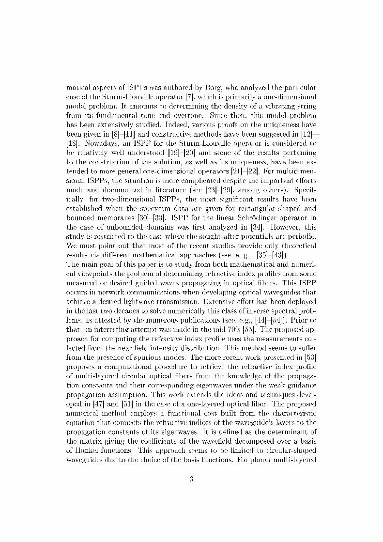
matical aspects of ISPPs was authored by Borg, who analyzed the particularcase of the Sturm-Liouville operator [7], which is primarily a one-dimensionalmodel problem. It amounts to determining the density of a vibrating stringfrom its fundamental tone and overtone. Since then, this model problemhas been extensively studied. Indeed, various proofs on the uniqueness havebeen given in [8][11] and constructive methods have been suggested in [12][18]. Nowadays, an ISPP for the Sturm-Liouville operator is considered tobe relatively well understood [19][20] and some of the results pertainingto the construction of the solution, as well as its uniqueness, have been ex-tended to more general one-dimensional operators [21][22]. For multidimen-sional ISPPs, the situation is more complicated despite the important eortsmade and documented in literature (see [23][29], among others). Specif-ically, for two-dimensional ISPPs, the most signicant results have beenestablished when the spectrum data are given for rectangular-shaped andbounded membranes [30][33]. ISPP for the linear Schrödinger operator inthe case of unbounded domains was rst analyzed in [34]. However, thisstudy is restricted to the case where the sought-after potentials are periodic.We must point out that most of the recent studies provide only theoreticalresults via dierent mathematical approaches (see, e. g., [35][43]).The main goal of this paper is to study from both mathematical and numeri-cal viewpoints the problem of determining refractive index proles from somemeasured or desired guided waves propagating in optical bers. This ISPPoccurs in network communications when developing optical waveguides thatachieve a desired lightwave transmission. Extensive eort has been deployedin the last two decades to solve numerically this class of inverse spectral prob-lems, as attested by the numerous publications (see, e.g., [44][54]). Prior tothat, an interesting attempt was made in the mid 70′s [55]. The proposed ap-proach for computing the refractive index prole uses the measurements col-lected from the near eld intensity distribution. This method seems to suerfrom the presence of spurious modes. The more recent work presented in [53]proposes a computational procedure to retrieve the refractive index proleof multi-layered circular optical bers from the knowledge of the propaga-tion constants and their corresponding eigenwaves under the weak guidancepropagation assumption. This work extends the ideas and techniques devel-oped in [47] and [51] in the case of a one-layered optical ber. The proposednumerical method employs a functional cost built from the characteristicequation that connects the refractive indices of the waveguide's layers to thepropagation constants of its eigenwaves. It is dened as the determinant ofthe matrix giving the coecients of the waveeld decomposed over a basisof Hankel functions. This approach seems to be limited to circular-shapedwaveguides due to the choice of the basis functions. For planar multi-layered

3

waveguides, the waveguide spectroscopy method is used in [44]. This methodconsists of minimizing the distance between the computed and the measuredpropagation constants vectors. The computed ones are obtained as the rootsof well-known characteristic equations. The application of this method hasbeen extended to waveguides with piecewise constant refractive index prolesand arbitrary cross-sectional boundaries [48], [50], [52], [53]. The authors pro-pose a strategy that is based on the solution of a nonlinear nonself-adjointeigenvalue problem corresponding to a system of weakly singular integralequations. The numerical approach introduced in [46] reconstructs the re-fractive index prole of a cylindrical waveguide from the knowledge of thecorresponding near eld in the case of Maxwell system. The main idea ofthis technique is to reformulate the problem into a set of one-dimensionalproblems after dividing the optical waveguide into homogeneous cylindri-cal layers of a prescribed thickness. The accuracy and eectiveness of themethod are highly dependent on the thickness parameter values. The workpresented in [54] seems very close to ours. However, the approach adoptedin [54] diers from our solution methodology by several aspects, chief amongthem: (a) the ISPP is formulated in [54] as an optimization problem underconstraints and is solved via the use of Lagrange multipliers, and (b) theFréchét derivatives with respect to the refractive index prole are computedusing a nite dierence (FD) approximation of order 1. Due to the con-straints considered in [54], the method is limited to continuous proles atthe interface core-cladding and its eciency (accuracy and convergence) issensitive to the FD step size value when approximating the derivatives.In the present work, we investigate the question of the uniqueness of thesolution for the considered ISPP and characterize its Fréchet derivative withrespect to the refractive index prole. At the numerical level, we proposea solution methodology that falls in the category of regularized iterativemethods. The proposed computational procedure possesses the followingfour main features: (a) a computationally ecient usage of the exact sen-sitivities of the guided modes to the specied refractive index parameters,(b) the solution of only one eigenvalue problem at each Newton iteration, (c)a Tikhonov-like regularization to restore the stability, and (d) an ecientcomputational method coupling a local boundary condition to a nite ele-ment formulation for solving the direct eigenvalue problem. Note that themathematical diculties, computational issues, and solution approaches ad-dressed in this paper are relevant to many ISPs arising in other applications.The remainder of this paper is organized as follows. In Section 2, we recallthe forward eigenvalue problem that characterizes the propagation of guidedmodes in a homogeneous optical ber. We assume the propagation to be un-der the weak guidance conditions [56][58]. In Section 3, we state the ISPP

4

of interest and establish mathematical results pertaining to (a) the unique-ness of the solution, and (b) the Fréchet derivative of the eigenmodes withrespect to the refractive index prole. Section 4 is devoted to the descrip-tion of the proposed solution methodology for solving the considered ISPP.We present in Section 5 various illustrative numerical results to highlight theperformance eciency of the proposed computational procedure. Concludingremarks are included in Section 6.

2 The Direct Problem

2.1 Nomenclature and assumptions

An optical ber can be viewed as a cylindrical dielectric structure that isextended along its propagation axis, denoted here by Ox3 (see Figure 1(a)).In its transverse directions, Ox1 and Ox2, an optical ber is constitutedof two open subsets of R2 : a core region denoted by Ω and a claddingregion Ωe = R2 \Ω (see Figure 1(b)). The core Ω is assumed to be Lipschitzcontinuous. The cladding Ωe is assumed to be innitely extended since guidedwaves decrease exponentially to zero out of the core region and the radiusof the cladding is in practice very large compared to the radius of bercore [56][59]. The core and the cladding regions are fully determined oncethe refractive index prole n of the considered ber is known. The proposedstudy is limited to optical bers with homogeneous cladding. Therefore, theclass of refractive index proles n we consider here are positive real-valuedfunctions depending on x = (x1, x2) such that n ∈ L∞(R2; R?

+), and:

∃ n∞ ∈ R?+ such that n(x) = n∞ a.e. x ∈ Ωe. (1)

Furthermore, to ensure the guided waves propagation in the considered ber,the refractive index prole must attain its maximum inside the core of theber [56][59], that is:

∃ n+ ∈ R?+ such that ess sup

x∈R2

n = n+ > n∞, (2)

where ess sup denotes the essential supremium [59].We consider the following class of refractive index proles:

N = n ∈ L∞(R2; R?+); ∃ n∞ > 0;

n(x) = n∞ a.e. in Ωe and ess supx∈R2

n = n+ > n∞, (3)

5

(a) (b)

Figure 1: (a) An optical ber, (b) a transverse section of a homogeneousoptical ber.

and the set of admissible refractive index proles considered in this study,denoted by N1, is dened by:

N1 = n ∈ N ; n being piecewise continuous (4)

Note that the set N1 encompasses all refractive index proles encountered inpractical applications [57][58], [60].

2.2 Problem statement

We consider the propagation of guided modes under the weak guidance condi-tions. Hence, we assume the refractive-index variations to be small comparedto the wavenumber k. In this situation, the propagation of guided waves inhomogeneous optical bers can be formulated as the following scalar eigen-value problem EVP [56][59]:

(EVP)

Find β ∈ ]kn∞, kn+[ and u ∈ L2(R2); u 6= 0 such that:

∆u+ k2n2u = β2u in R2 (5)

[u] =

[∂u

∂ν

]= 0 on Γ = ∂Ω, (6)

where:

• β is the propagation constant. It represents the speed of the electro-magnetic eld along its propagation axis Ox3 (see Figure 1(a)).

• u is the associated eigenfunction of β. It represents any transverse com-ponent of the electromagnetic eld that propagates in the ber. Thecouple (β, u) is called a guided mode.

6

• n is an admissible refractive index, that is, n ∈ N1.

• The brackets [ . ] in equation (6) represent the jump across the core-cladding interface Γ and ν is the unit normal vector on Γ oriented to-wards the cladding Ωe. The transmission conditions given by (6) expressthe continuity of the tangential components of the electromagnetic eldover the core-cladding interface Γ (see Figure 1(b)).

EVP has been analyzed extensively, both mathematically and numerically.Results pertaining to the existence of guided modes, their number, as wellas their sensitivities to the opto-geometrical parameters k and n of the con-sidered waveguide can be found in [56][59], among other references.

3 The Inverse Spectral Problem

3.1 Problem statement

As stated earlier in the introduction section, our aim is to propose a solu-tion methodology that eciently retrieves the refractive index prole fromthe knowledge of some guided modes (β, u) propagating, at a xed fre-quency, in a given optical ber. To formulate mathematically this inverseproblem, we rst recall that for a prescribed frequency, characterized bythe wavenumber k, and a given refractive index n ∈ N1, EVP admits a -nite number S of propagation constants, counted with their multiplicities,denoted by βS = (β1, · · · , βS)T and their corresponding eigenfunctions de-noted by uS = (u1, · · · , uS)T [59]. Therefore, EVP denes a vector-valuedmapping FS = (F1, F2, · · · , FS)T , such that:

FS : n −→ FS(n) = βS. (7)

Note that the lth coordinate Fl(n) = βl is the propagation constant corre-sponding to the lth guided mode, counted with its multiplicity. This meansthat the βls are not necessarily distinct. The considered inverse spectralproblem can be then formulated as follows:

(ISPP)

Given the rst I guided modes (β1, u1), (β2, u2), · · · , (βI , uI)(1 ≤ I ≤ S) propagating at a xed frequency k, nd the refrac-tive index n ∈ N1 such that:

FI(n) = βI = (β1, β2, · · · , βI)T . (8)

7

Remark. Note that the considered ISPP can also be extended to the casewhere the guided modes are measured for multiple frequencies correspond-ing to NF wavenumbers k1, k2, · · · , kNF

. For each considered wavenum-ber kl (1 ≤ l ≤ NF ), its corresponding rst Il propagation constants βIl =(β1l , β2l , · · · , βIl)T and their associated eigenfunctions uIl = (u1l , u2l , · · · , uIl)Tare given respectively in ISPP. Therefore, the number of eigenmodes I in ISPP

becomes I =

NF∑l=1

Il.

3.2 Mathematical results

The rst result establishes the uniqueness of the solution of ISPP.

Proposition 3.1. The refractive index n, solution of ISPP, can be uniquelydetermined in N1 from only the knowledge of the fundamental mode (β1, u1).

Proof. Consider ISPP with I = 1, that is the fundamental eigenmode pair(β1, u1) is given. Let n1 and n2 be two solutions of ISPP. Then, equation (5)implies:

∆u1 + k2n2l u1 = β2

1u1 in R2 with nl = nl,∞ > 0 in Ωe; l = 1, 2. (9)

It follows from the dierence between the two equations given by (9) that:

(n21 − n2

2) u1 = 0 a.e. in R2 (10)

In particular, we have:

(n1,∞ − n2,∞) u1 = 0 a.e. in Ωe, (11)

Hence, either u1 = 0 a.e. in Ωe or n1,∞ = n2,∞.

Case1: Assume that u1 = 0 a.e. in Ωe.Since u1 ∈ H2(R2) [59], then we have:

u1 =∂u1

∂ν= 0 a.e. on ∂Ωe (12)

and the standard trace theorems can be applied to u1 on the boundary forboth Dirichlet and Neumann traces. It follows that u1 satises the followinghomogeneous boundary value problem:

∆u1 + (k2n21 − β2

1)u1 = 0 in Ω

u1 =∂u1

∂ν= 0 on ∂Ω

8

Hence, using the unique continuation principle (see, e.g., [61][62]), we deducethat:

u1 = 0 a.e. in Ω,

and thereforeu1 = 0 a.e. in R2,

which contradicts u1 being an eigenfunction, i.e., ‖u1‖2 6= 0.

Case2: Assume that n1,∞ = n2,∞.If n1 6= n2, then, since the refractive index is a positive valued function, theremust be an open subset D ⊆ Ω, such that:

n21 − n2

2 6= 0 a.e. in D. (13)

It follows from the restriction of equation (10) to D that:∫D

(n21 − n2

2)2 u21 dx = 0, (14)

Consequently, we deduce from equations (13)-(14) that:

u1 = 0 a.e. in D. (15)

Using the same argument as in Case 1, we deduce that u1 = 0 a.e. in Dc =R2 \D and therefore u1 = 0 a.e. in R2, which contradicts u1 being an eigen-function (i.e., ‖u1‖2 6= 0).

Remark. The above proof suggests that the conclusion of Proposition 3.1is still valid when the considered fundamental mode (β1, u1) is replaced byany other pair of guided modes. The multiplicity of the propagation constantdoes not matter in the proof of the proposition.

The next result states that the previous uniqueness result is no longer validif the propagation constant value is given without the knowledge of the orderof the corresponding guided mode.

Proposition 3.2. The refractive index n, solution of ISPP, cannot be uniquelydetermined in N1 if the propagation constant β is given without its associatedeigeneld u.

Proof. In this situation, it is possible to prove the existence of a sequenceof refractive indices (nl)l ∈ N1, for which the considered β is the propa-gation constant of the corresponding lth mode. Indeed, observe that themapping F1 : n 7−→ β1(n) is an increasing function in the following sense:

9

for n, n′ ∈ N1, such that n ≥ n′, then F1(n) = β1(n) ≥ β1(n′) = F1(n′) [59].In addition, F1 is locally lipschitzian, and therefore continuous from N1

to R?+ [59]. Consequently, F1 denes a bijection from N1 to R?

+. This impliesthe existence of a unique refractive index n1 ∈ N1, solution of ISPP, suchthat β is the corresponding fundamental mode propagation constant.Similarly, since the mapping Fl, l ≥ 2, is also a bijection fromN1 into R?

+ [59],then we also prove the existence of a sequence of refractive indices (nl)l≥2

in N1 such that the considered β is also associated to their respective lth

guided mode.

We conclude this section by providing a characterization of the Fréchetderivative of the propagation constants with respect to the refractive index n.This result is relevant to the implementation of any Newton-type method forsolving ISPP. Indeed, it is well known that the accuracy and the eciencyof Newton-type methods strongly depend on the accuracy level in the com-putation of the jacobian matrix that occurs at each iteration.

Theorem 3.3. For a given wavenumber k, the Fréchet derivative of the map-ping Fl (1 ≤ l ≤ S), given by equation (7), with respect to the refractive indexprole n in the direction h ∈ L∞(R2; R?

+), when it exists, satises:

∂Fl∂n

(n)h =

k2

∫R2

nhu2l dx

βl

∫R2

u2l dx

. (16)

Proof. Since the guided mode pair (βl, ul) satises (5), then we apply thechain rule and obtain:

∆

(∂ul∂n

h

)+(k2n2 − β2

l

) ∂ul∂n

h+ 2

(k2nh− βl

∂βl∂n

h

)ul = 0 (17)

Next, we multiply equation (17) by ul and integrate over R2.We then obtain:∫R2

[∆

(∂ul∂n

h

)+(k2n2 − β2

l

) ∂ul∂n

h

]uldx+ 2

∫R2

(k2nh− βl

∂βl∂n

h

)u2l = 0

(18)Furthermore, we integrate equation (18) by parts and obtain:∫

R2

[∆ul +

(k2n2 − β2

l

)ul] ∂ul∂n

hdx+ 2

∫R2

(k2nh− βl

∂βl∂n

h

)u2l = 0 (19)

Note that, similarly to the derivation of the variational formulations in [63][64], equation (19) is obtained from (18) in two steps. We rst perform

10

the integration in the distribution sense. We then use the standard densityargument of D(R2) into H2(R2).Finally, it follows from equations (5) and (19) that∫

R2

(k2nh− βl

∂βl∂n

h

)u2l = 0, (20)

which concludes the proof of Theorem 3.3.

4 Solution Methodology

We propose a Tikhonov-regularized Newton procedure for solving ISPP [65][66], since regularized iterative methods appear to be the primary candidatesfor solving nonlinear and ill-posed problems (see, e.g., [67], and the referencestherein). The Newton algorithm addresses the nonlinear aspect of ISPP,whereas the Tikhonov regularization procedure is incorporated to address itsill-posed nature [68][69].

4.1 Parametrization

We assume that the sought-after refractive index prole n is in N1 and can beapproximated by a set of trial solutions given by the following parametriza-tion:

n(x) ≈NP∑m=1

αm gm(|x|) ; ∀x ∈ R2, (21)

where:

• the parameter NP is a positive integer representing the number of pa-rameters. NP is typically between 2 and 4, for most refractive indexproles of practical interest [60], [56][58]. Note that the numericalresults reported in [54] were obtained with NP = 2 and 3 only.

• the parameters α1, α2, · · · , αNPare real numbers. They represent the

unknown coecients to be determined.

• (gm)1≤m≤NPis a selected set of real-valued polynomial functions such

that:

i. For 1 ≤ m ≤ NP − 1, gm is a piecewise polynomial function ofdegree (m − 1), whose support is contained in the core Ω of theber.

11

ii. gNPis the characteristic function of the ber cladding, i.e., gNP

(x) =0 if x ∈ Ω and gNP

(x) = 1 elsewhere.

Basis functions for parametrizing respectively a refractive step-index proleand a refractive graded-index prole of a circular-shaped optical ber aredepicted in Figures 2 and 3, for illustrative purposes. Observe that it ispossible to employ other basis functions such as trigonometric or B-splinefunctions that are often encountered when solving inverse problems (see,e.g., [67]). This type of bases is more appropriate for refractive index prolesthat are not function of the radial direction r, but depend on x = (x1, x2),particularly for optical bers with arbitrary cross-sectional boundaries. Wehave adopted here these polynomial-type functions for mainly two reasons:

(a) The class of refractive index proles that we consider (see (3)-(4)) isalways piecewise continuous in Ω and constant in Ωc. Hence, thesefunctions appear to form an appropriate basis for approximating thisclass of proles.

(b) Since the proposed solution methodology employs a nite element methodfor solving the direct eigenvalue problem (see Section 4.3), the use ofpolynomial functions in the parametrization can be easily "blended" inthe nite element approximation without signicantly increasing thecomputational complexity of the method.

g (r)

raO

1

1

(a)

raO

g (r)2

1

(b)

Figure 2: Basis functions for parametrizing refractive step-index proles inthe case of a circular-shaped optical ber. NP = 2.

4.2 Newton iteration equation

Assume n(j) =

NP∑m=1

α(j)m gm to be the computed refractive index prole at

iteration j that approximates the solution n? of ISPP. Then, equation (8) is

12

g (r)

raO

1

1

(a)

g (r)

raO

1

2

(b)

raO

1

g (r)3

(c)

raO

1

g (r)4

(d)

Figure 3: Basis functions for parametrizing refractive graded-index prolesin the case of a circular-shaped optical ber. NP = 4.

replaced by the Newton iteration equation:

J(j)F δn(j) = βI − FI(n

(j)) (22)

where δn(j) is the update vector given by:

δn(j) =

NP∑m=1

δα(j)m gm (23)

and the updated index prole n(j+1) is given by:

n(j+1) = n(j) + δn(j), (24)

where J(j)F is the jacobian matrix of the operator FI = (F1, · · · , FI)T , eval-

uated at n(j), i.e.

J(j)F =

(∂β

(j)l

∂n

(n(j))gm

)1 ≤ l ≤ I1 ≤ m ≤ NP

. (25)

β(j)l = Fl(n

(j)) (1 ≤ l ≤ I) designates the propagation constant of the lth

guided mode, solution of EVP, for the refractive index prole n(j), and

13

(gm)1≤m≤NPis the considered basis of functions. The entries of the jaco-

bian matrix J(j)F are given, as stated in Theorem 3.3, by equation (16) in

which h is replaced by the basis functions gm, introduced in Paragraph 4.1(see Figures 2-3).Note that, at the algebraic level, if the number of parameters NP is equalto the number of the measurements I, then equation (22) is a square linearsystem. However, if NP is larger than I, the linear system (22) is rectan-gular. In this case, we solve this system in the least-squares sense, that is,equation (22) is replaced by:

JTF(j)

J(j)F δn(j) = JTF

(j) (βI − FI(n

(j))), (26)

where T stands for the transpose of a matrix. Last, since ISPP is an ill-posedproblem, we employ the standard Tikhonov regularized procedure to restorethe stability [68][69]. Therefore, we replace equation (22) or equation (26)by the following compact regularized Newton-type equation:(

E(j) J(j)F + µINP

)δn(j) = E(j)

(βI − FI(n

(j))), (27)

where E(j) is a NP × I matrix given by:

E(j) =

INP

if NP = I

JTF(j)

if NP > I,

(28)

and µ is a positive number called the regularized parameter. There arevarious strategies for selecting the "optimal" value of µ (see, e. g. [70][73]).Due to the small size of the resulting linear system, we propose a trial anderror strategy for nding the optimal value of µ. This consists in sweeping µover a large interval of positive real numbers and evaluating the residual foreach value of µ, and we then select the value of µ that leads to the minimumresidual (up to the noise level).

4.3 Ecient solver for the direct eigenvalue problem EVP

The proposed regularized Newton algorithm calls for the solution of the for-ward eigenvalue problem EVP. To this end, we employ the direct solver devel-oped in references [74][75]. This solver requires to rst reformulating EVP

14

in a bounded domain (see Figure 4(a)) as follows:

(EVP)

Find β ∈ ]kn∞, kn+[ and u ∈ L2(ΩΣ); u 6= 0 such that:∆u+ k2n2u = β2u in ΩΣ (29)

[u] =

[∂u

∂ν

]= 0 on Γ = ∂Ω (30)

∂u

∂ν+

(√β2 − k2n2

∞ +K2

)u = 0 on Σ = ∂ΩΣ , (31)

where K denotes the curvature of the employed articial boundary Σ. In theparticular case of Σ being a circular-shaped boundary of radius R, K = 1/R.Then, we apply a linear nite element approximation [76][77] to calculatethe solutions of the truncated eigenvalue problem EVP . This leads to thesolution of the following quadratic eigenvalue problem:

A x+ λ B x+√λ C x = 0 (32)

where:

• λ = β2 − k2n2∞ is the eigenvalue.

• x is the corresponding eigenvector. x ∈ RN with N being the numberof degrees of freedom of the FEM approximation.

• A, B, and C are symmetric matrices. A is the sum of a stiness ma-trix, a mass-like matrice, and a mass-like matrix on Σ that results fromthe term containing the curvature K in equation (31). B is a massmatrix and therefore B is positive denite. C is a mass-type matrixdened on Σ. C is a quasi-tridiagonal matrix.

To solve numerically the quadratic eigenvalue problem given by (32), wetransform it into a generalized eigenvalue problem of the form [74][75]:

A z =√λ B z (33)

where

A =

[−C −BA 0

]and

B =

[B 00 B

]We compute the pairs of eigensolutions

(√λ, z

)by employing the Implicitly

Restarted Arnoldi Method IRAM [78], which is an iterative algorithm of QR-type [79][80].

15

xO

2

1

Γ

x

Ω

2π /ka

Ω

Σ

Σ

(a) (b)

Figure 4: (a) The computational domain for a circular-shaped optical berand (b) an illustrative nite element mesh using triangular-shaped elements.

4.4 Algorithm summary

The proposed algorithm can be summarized as follows:

Step 0. Initialization. The proposed algorithm requires the followinginitial data:

• A prescribed shape of the core-cladding interface Γ = ∂Ω of the con-sidered optical ber.

• A set of NF wavenumbers k1, · · · , kNFdening the frequency regime

of the guided wave propagation.

• A set of the desired/measured guided modes that propagate in theconsidered ber for the respective prescribed wavenumbers kl, 1 ≤ l ≤NF . For each kl, its corresponding desired/measured guided modes arecharacterized by a set of pairs consisting of the propagation constantsand their corresponding guided elds, i.e., for each wavenumber kl, wehave the set of desired/measured pairs:(

β?1l , u?1l

),(β?2l , u

?2l

), · · · ,

(β?Il , u

?Il

), 1 ≤ l ≤ NF .

Note that these modes are listed with their multiplicities, i.e.

β?1l < β?2l ≤ β?3l ≤ · · · ≤ β?Il , 1 ≤ l ≤ NF .

The tilde indicates that the data (when measured) are possibly taintedwith errors.

16

• An initial parameter vector (n(0)1 , · · · , n(0)

NP) representing the initial

refractive index prole:

n(0) =

NP∑m=1

n(0)m gm

The admissible values of these parameters are arbitrarily selected, i.e.,they are "blind" guessed values.

Step 1. Apply Newton Iteration. This requires the accomplishment ofthe following three tasks, at the algorithm jth iteration (j = 0, 1, 2, · · · ):

i. Solve EVP with the refractive index n(j) and for each wavenumberkl, 1 ≤ l ≤ NF , to obtain a set of eigenpairs((

β(j)1l, u

(j)1l

), · · · ,

(β

(j)Il, u

(j)Il

))1≤l≤NF

.

ii. Evaluate the jacobian entries given by equation (25) using equation (16),the refractive index n(j), and the computed eigenpairs:((

β(j)1l, u

(j)1l

), · · · ,

(β

(j)Il, u

(j)Il

))1≤l≤NF

.

iii. Solve the regularized Newton iteration equation given by (27) to eval-uate δn(j) :(

E(j) J(j)F + µINP

)δn(j) = E(j)

(β?I − FI(n

(j))), (34)

where E(j) is given by (28).

Step 2. Stopping criteria. We monitor the convergence of the algorithmat iteration j (j = 0, 1, 2, · · · ) by evaluating both the relative residual onthe propagation constants:

Error1(j) =

(NF∑l=1

∣∣∣β?1l − β(j)1l

∣∣∣2 + · · ·+∣∣∣β?Il − β(j)

Il

∣∣∣2)1/2

(NF∑l=1

∣∣∣β?1l∣∣∣2 + · · ·+∣∣∣β?Il∣∣∣2

)1/2(35)

and the magnitude of the refractive index prole update:

max1≤m≤Np

∣∣δn(j)m

∣∣ (36)

17

We stop the algorithm at iteration j when one of these two values attainsa prescribed tolerance level ε. Note that we also evaluate, at each itera-tion j (j = 0, 1, 2, · · · ), the relative residual on the elds, i.e:

Error2(j) =

(NF∑l=1

∥∥∥u?1l − u(j)1l

∥∥∥2

2+ · · ·+

∥∥∥u?Il − u(j)Il

∥∥∥2

2

)1/2

(NF∑l=1

∥∥∥u?1l∥∥∥2

2+ · · ·+

∥∥∥u?Il∥∥∥2

2

)1/2(37)

This quantity is however used as a "discrimination" tool, i.e., to identify theorder of the computed modes as well as their corresponding polarization [56][58].

4.5 Computational complexity

The proposed solution methodology summarized in Paragraph 4.4 requires,at each Newton iteration, the following:

• The computation, for each considered wavenumber kl ( 1 ≤ l ≤ NF ),of the rst Il eigenpairs (β1l , u1l) , · · · , (βIl , uIl) . This is performedby applying IRAM algorithm (which is a QR-type method) [78] to ageneralized eigenvalue system whose size is 2N × 2N, where N is thenumber of degrees of freedom of the FEM approximation. Note thatthe application of IRAM calls for solving non-symmetric linear systems,which is accomplished using GMRES procedure [79].

• The computation of the jacobian entries, for each considered wavenum-ber kl ( 1 ≤ l ≤ NF ), by evaluating NP × Il integrals. This can beperformed using a Gauss-type quadrature [81][82]. However, sincewe have employed an "overkill" mesh for solving the direct eigenvalueproblem EVP, the size of the triangles is very small compared to thevariations of the integrands. Hence, it appears reasonable to assumethe integrand over each FEM triangle to be constant and equal to theaverage of its values on the nodes of the considered triangle. The ob-tained results indicate that this simple procedure is very accurate andcost-eective.

• The determination of the prole update δn by solving a small NP ×NP

linear system that can be executed analytically by simply applying adirect method [83]. However, in this work, we inverted this system

18

analytically when the order of parameter NP is either 2 or 3 (see Sec-tions 5.1 and 5.2). Consequently, we have observed that µ = 0 is theoptimal value of the regularization parameter, i.e., there is no need toregularize since the inversion is analytically performed and thereforeis "exact" when the number of the sought-after parameters is less orequal to 3. On the other hand, when NP = 5 or 6 (see Section 5.3),the algorithm does not converge without regularization.

5 Illustrative Numerical Results

We present numerical results to illustrate the potential of the proposed New-ton algorithm for eciently determining the refractive index prole from theknowledge of some guided modes. These results were obtained in the case ofan optical ber whose core-cladding interface Γ is a circular-shaped boundary(see Figure 4(a)). In all of the numerical experiments, we set the radius aof Γ to be a = 0.4µm and we use only one frequency whose wavenumberis k = 5 × 106 m−1. Note that we have xed the values of these two opto-geometric parameters so that we can use the same nite element resolutionin all experiments, i.e., there is no need to generate a new mesh. On theother hand, the refractive index prole parameters n+ and n∞ will havetheir values changed to ensure that the value of the normalized frequencyV = ka

√n2

+ − n2∞ is suciently large to allow the needed number of guided

modes to propagate in the ber [84][85]. Furthermore, we use the followingdiscretization parameters:

• The exterior articial boundary Σ is circular-shaped of radius R and islocated at one wavelength from the core-cladding interface Γ (see Fig-ure 4(a)). This distance is considered to be far enough to prevent anyreections, as demonstrated in references [74][75].

• We use a linear nite element approximation with 50 elements perwavelength. This discretization appears to be ne enough to ensurethe computation of the guided modes with a high accuracy level [74][75].

In what follows, we present results for determining three major classes ofrefractive index proles that are of practical interest: step-index, graded-index, and W-refractive index proles [56][58], [60], [84].

19

5.1 Retrieving refractive step-index proles

The goal of this section is to determine the parameters corresponding to arefractive step-index prole. To this end, we consider the class of refractiveindex proles of the form:

n(x) =

n+ ; x ∈ Ωn∞ ; x ∈ Ωe.

(38)

We present the results of two numerical experiments. In the rst one, thegoal is to determine the refractive index of the core of the ber only, whereasin the second one, we recover both indices. We must point out that themeasured guided modes are synthetic data obtained by solving the followingdispersion equation (see equation (A9), page 1574, in reference [74]):

λ1Jν+1(λ1)

Jν(λ1)= λ2

Kν+1(λ2)

Kν(λ2); ν = 0, 1, 2, · · · (39)

where λ1 = a√k2n2

+ − β2 and λ2 = a√β2 − k2n2

∞. Jν (resp. Kν) is theBessel function (resp. the modied Bessel function) of the rst kind [81].

5.1.1 Experiment 1: Partial parameters recovery

The goal of this experiment is to retrieve one refractive index parameterfrom the knowledge of one pair of guided modes. We choose the unknownrefractive index prole parameter to be n+, the refractive index of the coreof the ber, and we assume that:

n+ − n∞ = 0.01. (40)

This means that we consider here a one-parameter inverse problem. Thetarget refractive index prole value is n?+ = 50.005 whereas the initial value

is n(0)+ = 200.005. The measured guided mode corresponding to the target

prole n?+ is the fundamental mode LP01 [56][58] whose propagation con-stant, computed from equation (39), is:

β?1 = 249.996 (41)

The initial propagation constant value corresponding to the initial refractiveindex prole n(0) is:

β(0)1 = 1000.014. (42)

We also assess the sensitivity of the performance eciency of the proposedalgorithm to the noise level in the data. To this end, the propagation con-stant β?1 was respectively tainted with three dierent levels of white noise:

20

5%, 10% and 20%. Note that the noisy values are denoted by β?1 . The re-sults are reported in Table 1 and Figures 5-6. The following observations arenoteworthy:

• The initial value of the refractive index parameter is selected outsidethe pre-asymptotic convergence region. Indeed, the relative error onthe refractive index prole is about 300%. In addition, equations (41)-(42) show that the use of this initial guess leads to the computationof a propagation constant with relative residuals ranging from 200%to 300%, depending on the noise level. Furthermore, as indicated in Fig-ures 6(a) and 6(b), the isovalues of the exact eld vary between 0.0002and 0.037, whereas the ones corresponding to the initial guess rangebetween 1.06× 10−7 and 0.05. Clearly, Experiment 1 is performed witha "blind" initial guess value n?+.

• Figure 5 illustrates the fast convergence and the robustness to the noiseeect of the proposed solution methodology. More specically, onecan observe that the relative residual drops from the initial value ofover 200% to about the noise level in -at most- 3 iterations, for all con-sidered noise levels. In addition, Figure 5 reveals that the convergenceis monotone with almost no oscillations. This unusual behavior whensolving inverse-type problems is most likely due to the fact that thealgorithm is applied to a one-parameter inverse problem and thereforethe instability eects, if any, seem to be barely noticeable.

• At convergence, the refractive index parameter n+ is delivered with anaccuracy up to the noise level (see Table 1). On the other hand, Ta-ble 1 indicates that the proposed algorithm delivers the guided eld u1

with an excellent accuracy level even when the noise level is 20% (seeFigure 6).

21

Initial Relative Relative Relative Relativenoise level residual (%) error error erroron β?1(%) on n? (%) on β?1 (%) on u?1 (%)

0 0.852 0.852 0.852 0.3085 3.042 8.193 8.194 3.06310 2.734 13.005 13.007 4.70120 2.229 22.671 22.675 7.667

Table 1: Sensitivity of the relative residual and the relative error, at conver-gence, to the noise level for Experiment 1.

0

50

100

150

200

250

300

0 2 4 6 8 10

Rel

ativ

e re

sid

ual

(%

)

Iteration Number

(a) Noise free

0

50

100

150

200

250

300

0 2 4 6 8 10

Rel

ativ

e re

sid

ual

(%

)

Iteration Number

(b) Noise level 5%.

0

50

100

150

200

250

0 2 4 6 8 10

Rel

ativ

e re

sid

ual

(%

)

Iteration Number

(c) Noise level 10%.

0

50

100

150

200

250

0 2 4 6 8 10

Rel

ativ

e re

sid

ual

(%

)

Iteration Number

(d) Noise level 20%.

Figure 5: Convergence history. Sensitivity of the relative residual given byequation (35) to the noise level on the propagation constant β?1 .

22

(a) Analytical (b) Initial

(c) Computed with noise free (d) Computed with 5% noise level

(e) Computed with 10% noise level (f) Computed with 20% noise level

Figure 6: Isovalues corresponding to the fundamental mode LP01. Analyticvs. computed elds for various noise levels on β?1 .

23

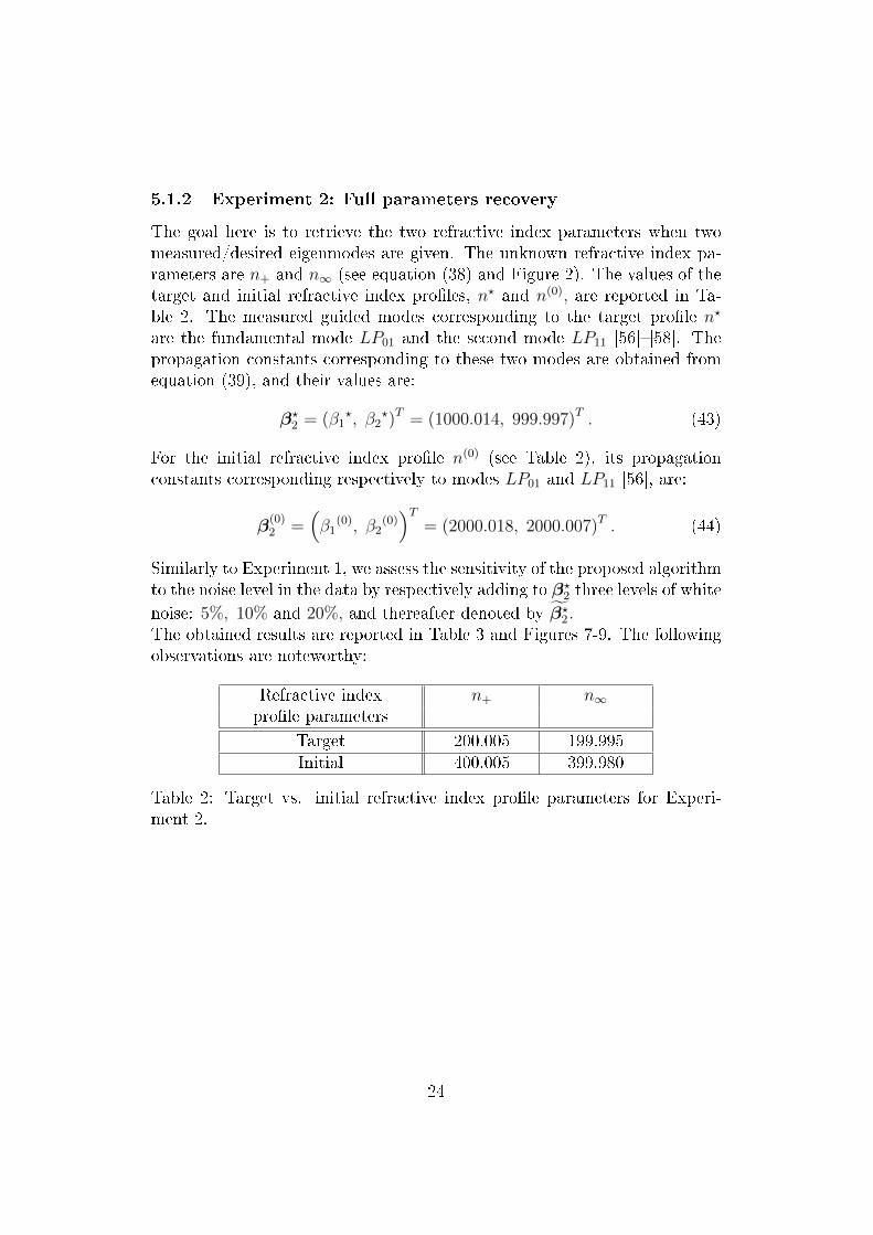
5.1.2 Experiment 2: Full parameters recovery

The goal here is to retrieve the two refractive index parameters when twomeasured/desired eigenmodes are given. The unknown refractive index pa-rameters are n+ and n∞ (see equation (38) and Figure 2). The values of thetarget and initial refractive index proles, n? and n(0), are reported in Ta-ble 2. The measured guided modes corresponding to the target prole n?

are the fundamental mode LP01 and the second mode LP11 [56][58]. Thepropagation constants corresponding to these two modes are obtained fromequation (39), and their values are:

β?2 = (β1?, β2

?)T = (1000.014, 999.997)T . (43)

For the initial refractive index prole n(0) (see Table 2), its propagationconstants corresponding respectively to modes LP01 and LP11 [56], are:

β(0)2 =

(β1

(0), β2(0))T

= (2000.018, 2000.007)T . (44)

Similarly to Experiment 1, we assess the sensitivity of the proposed algorithmto the noise level in the data by respectively adding to β?2 three levels of white

noise: 5%, 10% and 20%, and thereafter denoted by β?2.The obtained results are reported in Table 3 and Figures 7-9. The followingobservations are noteworthy:

Refractive index n+ n∞prole parameters

Target 200.005 199.995Initial 400.005 399.980

Table 2: Target vs. initial refractive index prole parameters for Experi-ment 2.

24

Initial Relative Relative Relative Relative Relativenoise level residual (%) error error error erroron β?2(%) on n? (%) on β?2 (%) on u?1(%) on u?2(%)

0 0.0 4.349× 10−5 0.0 0.18468 1.266725 2.926× 10−5 4.999 5.0 5.19346 7.8399310 8.864× 10−5 9.999 10.0 9.21879 13.3507020 6.732× 10−5 19.989 20.0 22.15990 28.71202


0

20

40

60

80

100

0 2 4 6 8 10

Rel

ativ

e re

sid

ual

(%

)

Iteration Number

(a) Noise free

0

20

40

60

80

100

0 2 4 6 8 10

Rel

ativ

e re

sid

ual

(%

)

Iteration Number

(b) Noise level 5%.

0

20

40

60

80

0 2 4 6 8 10

Rel

ativ

e re

sid

ual

(%

)

Iteration Number


-10

0

10

20

30

40

50

60

70

0 2 4 6 8 10

Rel

ativ

e re

sid

ual

(%

)

Iteration Number


Figure 7: Convergence history. Sensitivity of the relative residual given byequation (35) to the noise level on the propagation constants β?2 for Experi-ment 2.

25


(c) Computed with 0% noise level (d) Computed with 5% noise level


Figure 8: Isovalues corresponding to the guided mode LP x111 . Analytic vs.

computed elds for various noise levels on β?2 for Experiment 2.

26




Figure 9: Isovalues corresponding to the guided mode LP x211 . Analytic vs.


• Similarly to Experiment 1, the initial values of the refractive index pa-rameters are selected outside the pre-asymptotic convergence region,since the relative error on the refractive index prole is 100% (see Ta-

27

ble 2). Moreover, this initial guess leads to the computation of prop-agation constants with relative residuals ranging from 67% to 100%,depending on the level of noise (see equations (43)-(44)). This is alsoillustrated by the important dierence in the values of the correspond-ing eigenmodes. Indeed, for example, the isovalues for the exact LP11

eld vary between −0.049 and 0.049, whereas the ones correspondingto the initial guess range between −0.058 and 0.058, as indicated inFigures 8(a)8(b) and Figures 9(a)9(b). Hence, this experiment isclearly performed with a "blind" initial guess value.

• Figure 7 illustrates the fast convergence and the robustness to thenoise eect of the proposed solution methodology. More specically,one can observe that the relative residual drops from the initial valueof over 67%, to below the noise level after one iteration only, for allconsidered noise levels. Furthermore, Figure 7 clearly shows that theconvergence is almost monotone with almost no oscillations. This be-havior is most likely due to the fact that the algorithm is applied toa two-parameter problem, and therefore, the instability eects seem tobe negligible.

• At convergence, the refractive index parameters (n+, n∞) are deliveredwith an accuracy up to the noise level (see Table 3). The correspondingguided elds (u1, u2) are also computed with a satisfactory accuracylevel (see Table 3 and Figures 8-9).

5.2 Retrieving a refractive graded-index prole

The goal of this section is to determine the parameters corresponding to arefractive graded-index prole. To this end, we consider the class of refractiveindex proles of the form:

n(x) =

n+ + α.|x|2 ; x ∈ Ωn∞ ; x ∈ Ωe,

(45)

and satisfying:0 < n+ − n∞ ≤ 0.01. (46)

Hence, the propagation of the modes is under the weak guidance condi-tions [56][59]. In what follows, we present the results of two numericalexperiments. In the rst experiment, the goal is to determine the value ofthe refractive index at the center of the ber core n+, as well as in thecladding n∞. In the second experiment, we recover the indices of both thecore (n+, α) and the cladding n∞.

28

5.2.1 Experiment 3: Partial parameters recovery

The goal here is to retrieve two refractive index parameters, given two mea-sured/desired eigenmodes. The unknown refractive index parameters are n+

and n∞ (see equation (45) and Figure 2). Moreover, the value of the pa-rameter α ∈ R in equation (45) is chosen to ensure the continuity of therefractive graded-index prole across the interface core-cladding. Therefore,α is a parameter that depends on n+ and n∞. Consequently, we considerhere a two-parameter inverse problem. The values of the target and initialrefractive index proles, n? = (n?+, n

?∞) and n(0) = (n

(0)+ , n

(0)∞ ), are reported

in Table 4 as well as the resulting values of α for both proles. The measuredguided modes corresponding to this prole are the fundamental mode LP01

and the second mode LP11 [56][58]. The values of propagation constantsobtained with the nite element solver [74][75] are given by:

β?2 = (β1?, β2

?)T = (2250.008, 2249.992)T . (47)

For the initial refractive index prole n(0) (see Table 4), its propagationconstants corresponding respectively to modes LP01 and LP11, obtained fromthe dispersion equation (39), are:

β(0)2 =

(β1

(0), β2(0))T

= (4000.005, 3999.985)T . (48)

We assess the sensitivity of the proposed algorithm to the noise level in β?2,by respectively adding to it three levels of white noise: 5%, 10% and 20%,and thereafter denote the noisy β?2 by β?2.The results are reported in Table 5 and Figures 10-??. The following obser-vations are noteworthy:

Refractive index n+ n∞ αprole parameters

Target 450.005 449.995 -0.06250Initial 800.005 799.980 -0.15625


29

Initial Relative Relative Relative Relative Relativenoise level residual (%) error error error erroron β?2(%) on n? (%) on β?2 (%) on u?1(%) on u?2(%)

0 1.284× 10−3 2.874× 10−3 1.284× 10−3 0.46894 1.688055 1.124× 10−3 4.998 4.999 4.91770 6.8139310 9.397× 10−4 9.998 9.999 9.93758 12.4969720 6.587× 10−4 19.998 19.999 18.29067 22.12093


0

20

40

60

80

0 2 4 6 8 10

Rel

ativ

e re

sid

ual

(%

)

Iteration Number

(a) Noise level on β = (β1, β2) : 0%.

-10

0

10

20

30

40

50

60

70

80

0 2 4 6 8 10

Rel

ativ

e re

sid

ual

(%

)

Iteration Number

(b) Noise level on β = (β1, β2) : 5%.

-10

0

10

20

30

40

50

60

70

0 2 4 6 8 10

Rel

ativ

e re

sid

ual

(%

)

Iteration Number

(c) Noise level on β = (β1, β2) : 10%.

0

10

20

30

40

50

60

0 2 4 6 8 10

Rel

ativ

e re

sid

ual

(%

)

Iteration Number

(d) Noise level on β = (β1, β2) : 20%.


• The initial values of the refractive index parameters are chosen out-side the pre-asymptotic convergence region. Indeed, the initial relative

30

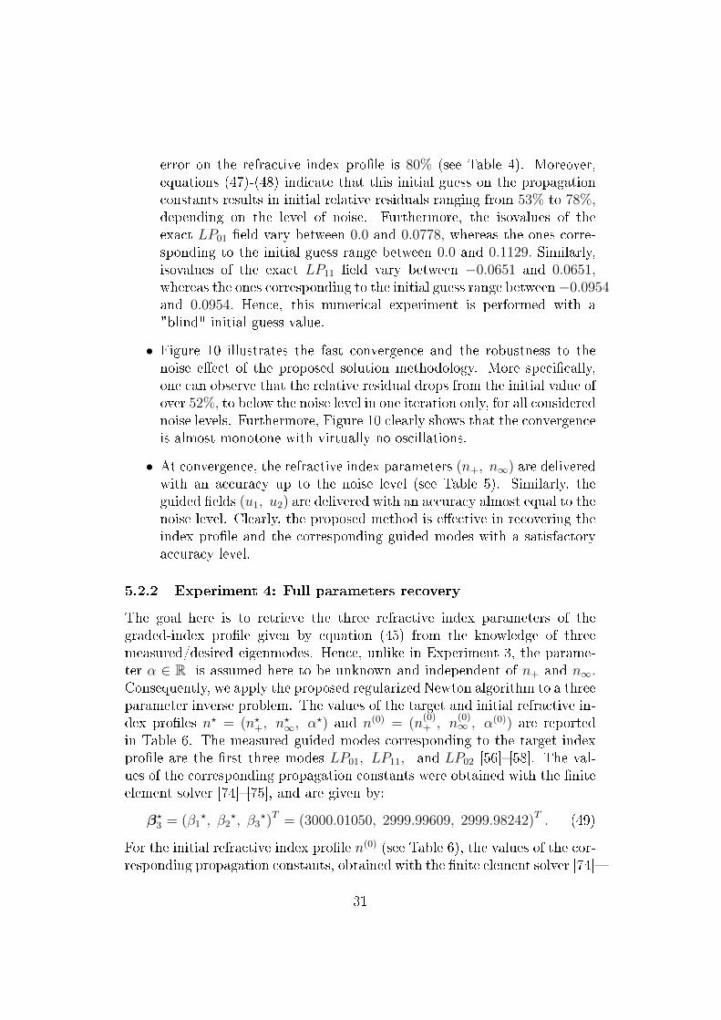
error on the refractive index prole is 80% (see Table 4). Moreover,equations (47)-(48) indicate that this initial guess on the propagationconstants results in initial relative residuals ranging from 53% to 78%,depending on the level of noise. Furthermore, the isovalues of theexact LP01 eld vary between 0.0 and 0.0778, whereas the ones corre-sponding to the initial guess range between 0.0 and 0.1129. Similarly,isovalues of the exact LP11 eld vary between −0.0651 and 0.0651,whereas the ones corresponding to the initial guess range between−0.0954and 0.0954. Hence, this numerical experiment is performed with a"blind" initial guess value.

• Figure 10 illustrates the fast convergence and the robustness to thenoise eect of the proposed solution methodology. More specically,one can observe that the relative residual drops from the initial value ofover 52%, to below the noise level in one iteration only, for all considerednoise levels. Furthermore, Figure 10 clearly shows that the convergenceis almost monotone with virtually no oscillations.

• At convergence, the refractive index parameters (n+, n∞) are deliveredwith an accuracy up to the noise level (see Table 5). Similarly, theguided elds (u1, u2) are delivered with an accuracy almost equal to thenoise level. Clearly, the proposed method is eective in recovering theindex prole and the corresponding guided modes with a satisfactoryaccuracy level.

5.2.2 Experiment 4: Full parameters recovery

The goal here is to retrieve the three refractive index parameters of thegraded-index prole given by equation (45) from the knowledge of threemeasured/desired eigenmodes. Hence, unlike in Experiment 3, the parame-ter α ∈ R is assumed here to be unknown and independent of n+ and n∞.Consequently, we apply the proposed regularized Newton algorithm to a threeparameter inverse problem. The values of the target and initial refractive in-dex proles n? = (n?+, n

?∞, α

?) and n(0) = (n(0)+ , n

(0)∞ , α(0)) are reported

in Table 6. The measured guided modes corresponding to the target indexprole are the rst three modes LP01, LP11, and LP02 [56][58]. The val-ues of the corresponding propagation constants were obtained with the niteelement solver [74][75], and are given by:

β?3 = (β1?, β2

?, β3?)T = (3000.01050, 2999.99609, 2999.98242)T . (49)

For the initial refractive index prole n(0) (see Table 6), the values of the cor-responding propagation constants, obtained with the nite element solver [74]

31

[75], are:

β(0)3 =

(β1

(0), β2(0), β3

(0))T

= (5000.0068, 4999.989, 4999.971)T . (50)

We assess the sensitivity of the proposed algorithm to the noise level in β?3,by adding to it three levels of white noise: 5%, 10% and 20%, and thereafterdenote the noisy β?3 by β?3.The obtained results are reported in Table 7 and Figures 11-12. The followingobservations are noteworthy:

Refractive index n+ n∞ αprole parameters

Target 600.005 599.995 -0.06250Initial 1000.005 999.980 -0.15625


Ini. noise Relative Relative Relative Relative Relative Relativelevel on residual error on error on error on error on error onβ?3(%) (%) n? (%) β?3 (%) u?1(%) u?2(%) u?3(%)

0 4.70E−6 1.02E−5 4.70E−6 0.383 1.624 0.7235 3.52E−5 5.0 5.0 2.448 3.211 3.06410 3.63E−5 10.0 10.0 9.223 9.422 9.69520 0.0 20.0 20.0 17.983 19.016 51.547


32

-10

0

10

20

30

40

50

60

70

0 2 4 6 8 10

Rel

ativ

e re

sid

ual

(%

)

Iteration Number

(a) Noise free

-10

0

10

20

30

40

50

60

0 2 4 6 8 10

Rel

ativ

e re

sid

ual

(%

)

Iteration Number

(b) Noise level 5%.

-10

0

10

20

30

40

50

60

0 2 4 6 8 10

Rel

ativ

e re

sid

ual

(%

)

Iteration Number


0

10

20

30

40

0 2 4 6 8 10

Rel

ativ

e re

sid

ual

(%

)

Iteration Number



• Similarly to the previous experiments, the initial values of the refractiveindex parameters are selected outside the pre-asymptotic convergenceregion. Indeed, the initial relative error on the refractive index proleparameters (see Table 6) is about 66.7%. This initial guess leads to thecomputation of propagation constants with relative residuals rangingfrom 39% to 67%, depending on the noise level (see equations (49)-(50)). Moreover, the isovalues of the exact modes are signicantly dif-ferent from the initial ones. For example, the isovalues of the exact LP02

eld vary between −0.035 and 0.077, whereas the ones correspondingto the initial guess range between −0.066 and 0.116, as indicated inFigures 12(a)12(b). Hence, this experiment is clearly performed witha "blind" initial guess value.

• Figure 11 illustrates the fast convergence and the robustness to the

33




Figure 12: Isovalues corresponding to the guided mode LP02. Analytic vs.computed elds for various noise levels on β?3 for Experiment 4.

noise eect of the proposed solution methodology. More specically,one can observe that the algorithm converges after only one iteration,for all considered noise levels (see the second column in Table 7). Fur-

34

thermore, Figure 11 clearly shows that the convergence is almost mono-tone with almost no oscillations.

• At convergence, the relative error on refractive index parameters n? =(n?+, n

?∞, α

?) is comparable to the noise level. Table 7 indicates thecorresponding propagation constants β?3 as well as the associated eigen-functions u?1 and u

?2 are obtained with relative errors comparable to the

noise levels. This remark is also valid for the associated eigenfunc-tion u?3, except when the noise level in the data is 20%. This might bedue to the fact that the eigenmode LP02 is very close to the cut-ofrequency [56][58], and therefore very sensitive to a relatively largeperturbation on the value of the propagation constant β?3 .

5.3 Retrieving W-shaped refractive index proles

Next, we consider a third class of refractive index proles, namely the W-refractive index proles, that is important to many applications [56][58], [60].This class of proles is very eective for reducing the modal dispersion eectand for enhancing the bandwidth performance of the optical bers [60]. Thisclass of proles is given by the following power law [60]:

n(x) =

n+

√1− 2ρ∆

(|x|a

)g; 0 ≤ |x| ≤ a

n∞ ; |x| ≥ a

(51)

where

• ∆ is a positive number representing the refractive index dierence. ∆is given by:

∆ =n2

+ − n2∞

2n2+

(52)

• g is a positive number, called the index component. It determines therefractive index proles.

• ρ is a positive number representing the depth of the index valley, asshown in Figure 13(a), Figure 17(a), and Figure 20(a). Observe thatwhen ρ = 1, the prole index given by (51) falls in the category of thegraded refractive index proles similar to the one considered in Sec-tion 5.2.

The goal here is to use the index prole parametrization given by (21) andapply the proposed algorithm to retrieve proles given by (51) in the case

35

where ρ = 1.7 and g = 2. The practical performance of this set of proleshas been analyzed in [60]. We investigate the sensitivity of the reconstruc-tion to the number of parameters NP in (21). We present results obtainedfor NP = 4 and NP = 5. We also present reconstruction results with NP = 3to demonstrate that when some a priori knowledge about the target proleis available, one can use fewer parameters.

5.3.1 Experiment 5: Retrieving a W-refractive index prole with

four parameters

The goal here is to determine the prole depicted in Figure 13(a) from theknowledge of its rst four guided modes LP01, LP11, LP02, and LP21. Thesesynthetic four guided modes were delivered by the nite element solver in-troduced in Section 4.3. The corresponding propagation constants valuesobtained with the nite element solver [74][75] are:

β?4 = (7562.51270, 7562.50098, 7562.48877, 7562.48877)T . (53)

We use the parametrization given by (21) with NP = 4 and the basis func-tions gl1≤l≤4 , depicted in Figure 3. Hence, we consider a four-parameterinverse problem whose unknowns are α1, α2, α3 and α4. Similarly to the pre-vious experiments, we taint the propagation constants vector β?4 with 3 noiselevels: 5%, 10% and 20%. The initial index prole n(0) is a step-index proledepicted in Figure 13(b), whose parameters are: α

(0)1 = 2512.505, α

(0)2 =

α(0)3 = 0, and α

(0)4 = 2512.495. The rst four propagation constants corre-

1512.490

1512.495

1512.500

1512.505

0 0.2 0.4 0.6 0.8 1

n(r

)

r=|x|

(a) Target prole: W-shape

2512.495

2512.500

2512.505

0 0.2 0.4 0.6 0.8 1

n(r

)

r=|x|

(b) Initial prole: step-index

Figure 13: Refractive index prole in Experiment 5: Target vs. initial.

sponding to n(0) are:

β(0)4 = (12562.5234, 12562.5215, 12562.5186, 12562.5176)T , (54)

36

For each noise level in the measured propagation constants vector β?4, weapply the proposed inversion algorithm from the initial step index prole n(0)

to determine the W-refractive index depicted in Figure 13(a). The resultsare reported in Figures 1416. The following observations are noteworthy:

• The algorithm is initiated outside the pre-asymptotic convergence re-gion. Indeed, the initial refractive index prole is a step-index prolethat signicantly diers from the target prole which is a W-shapeprole (see Figure 13). The relative error between the two prolesis over 66%. Moreover, the initial relative residual on the propagationconstants vector is about 67%. The corresponding initial eigenelds arealso very dierent from the ones corresponding to the W-shape prole,as illustrated in Figures 16(a)16(b) for the mode LP x2

21 .

• Similarly to the previous experiments, the convergence of the proposedalgorithm is relatively very fast, as demonstrated in Figure 14. We mustpoint out that in this case the regularization was critical to ensure theconvergence of the algorithm.

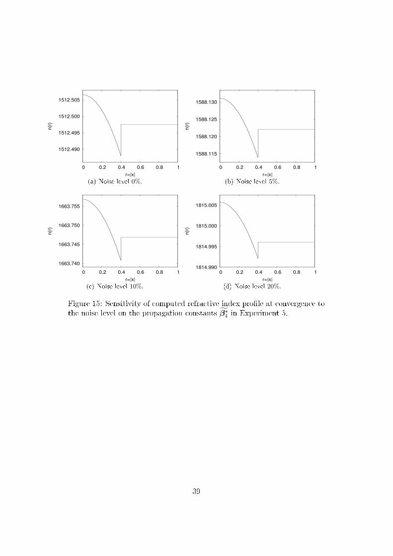
• Figure 15 shows that, at convergence, the sought-after refractive indexprole is delivered with an accuracy ranging from 10−5% (in the absenceof noise) to about 20% when the noise level is 20%. The recovery ofthe W-shape prole appears to be quite satisfactory, as illustrated inFigure 16 in which the mode LP x2

21 is depicted. The relative error variesfrom 4% to 18%, depending on the noise level.

37

0

10

20

30

40

50

60

70

0 2 4 6 8 10

Re

lative

re

sid

ua

l (%

)

Iteration number

(a) Noise free

0

10

20

30

40

50

60

0 2 4 6 8 10

Re

lative

re

sid

ua

l (%

)

Iteration number

(b) Noise level 5%.

0

10

20

30

40

50

0 2 4 6 8 10

Re

lative

re

sid

ua

l (%

)

Iteration number


-5

0

5

10

15

20

25

30

35

40

0 2 4 6 8 10

Re

lative

re

sid

ua

l (%

)

Iteration number



38

1512.490

1512.495

1512.500

1512.505

0 0.2 0.4 0.6 0.8 1

n(r

)

r=|x|

(a) Noise level 0%.

1588.115

1588.120

1588.125

1588.130

0 0.2 0.4 0.6 0.8 1

n(r

)

r=|x|

(b) Noise level 5%.

1663.740

1663.745

1663.750

1663.755

0 0.2 0.4 0.6 0.8 1

n(r

)

r=|x|


1814.990

1814.995

1815.000

1815.005

0 0.2 0.4 0.6 0.8 1

n(r

)

r=|x|


Figure 15: Sensitivity of computed refractive index prole at convergence tothe noise level on the propagation constants β?4 in Experiment 5.

39

(a) Target (b) Initial



Figure 16: Isovalues corresponding to the guided mode LP x221 . Target vs.



ve parameters

The main objective in this experiment is to investigate the eect of increasingthe number of parameters in the approximation given by (21) on the per-

40

formance (convergence and accuracy) of the proposed inversion algorithm.To this end, we consider a vector of ve measured propagation constantscorresponding to the modes LP01, LP11, LP02, LP21, LP12. The syntheticvector β?5 computed with the nite element solver [74][75], is given by:

β?5 = (9000.01367, 9000.00293, 8999.99219, 8999.99219, 8999.98145)T

(55)and corresponding to the sought-after W-refractive index prole depicted inFigure 17(a). We use the parametrization given by (21) with NP = 5. Notethat we also employ the basis functions depicted in Figure 3, but with g4 beingthe polynomial function of degree 3 extended by 0 for r ≥ a, and g5 being thefunction depicted in Figure 3(d). We thus consider a ve-parameter inverseproblem whose unknowns are αj, j = 1, · · · , 5. Similarly to Experiment 5,measurements are contaminated with the same noise levels. The initial indexprole n(0) is also a step-index prole (see Figure 17(b)) whose rst vepropagation constants, obtained with the nite element solver [74][75], are:

β(0)5 = (14250.0234, 14250.0215, 14250.0195, 14250.0186, 14250.0166)T (56)

For each noise level in the measured propagation constants vector β?5, weapply the proposed algorithm from the initial step-index prole n(0) to deter-mine the W-refractive index prole in Figure 17(a). The results are reportedin Figures 18??. These results reveal the following:

• Similarly to Experiment 5, the algorithm is initiated from a refractiveindex prole (a step index) that signicantly diers from the targetprole (W-shape), as indicated in Figure 17. The initial relative erroris about 60%, resulting in an initial relative residual of also about 60%.Clearly, the inversion algorithm is initiated outside the pre-asymptoticregion.

• Figure 18 shows that the convergence of the algorithm is comparableto the one observed in Experiment 5 when using only 4 parameters. Inaddition, the algorithm does not converge without incorporating theregularization procedure.

• The sought-after refractive index prole is determined with an accuracylevel comparable to the case of 4 parameters. Indeed, at convergence,the relative error on the refractive index prole ranges from 10−5%(in the absence of noise) to about 20% when the noise level is 20%.On the other hand, we observed an improvement in the accuracy ofthe corresponding eigenmodes. For example, the highest mode LP12 is

41

1799.990

1799.995

1800.000

1800.005

0 0.2 0.4 0.6 0.8 1

n(r

)

r=|x|

(a) Target prole: W-shape

2849.995

2850.000

2850.005

0 0.2 0.4 0.6 0.8 1

n(r

)

r=|x|

(b) Initial prole: step-index


computed with a relative error ranging from 8.5% to 11% dependingon the noise level.

42

0

10

20

30

40

50

60

0 2 4 6 8 10

Re

lative

re

sid

ua

l (%

)

Iteration number

(a) Noise free

0

10

20

30

40

50

0 2 4 6 8 10

Re

lative

re

sid

ua

l (%

)

Iteration number

(b) Noise level 5%.

0

10

20

30

40

0 2 4 6 8 10

Re

lative

re

sid

ua

l (%

)

Iteration number


-5

0

5

10

15

20

25

30

35

0 2 4 6 8 10

Re

lative

re

sid

ua

l (%

)

Iteration number




three parameters

The goal of this experiment is to demonstrate that when some a priori knowl-edge on the sought-after prole is available, it is possible to successfullyrecover the prole using fewer parameters in (21). For this numerical ex-periment, The target prole (W-refractive) is depicted in Figure 20(a). Weemploy the parametrization given by (21) with NP = 3. Note that the g1 isthe constant depicted in Figure 3(a), g2 is the quadratic polynomial func-tion depicted in Figure 3(c), and g3 is the constant function depicted inFigure 3(d). Hence, we assume a priori that this set of trial solutions can de-scribe the sought-after W-prole. The synthetic measurements are the rstguided modes LP01, LP11, and LP02 whose propagation constants are:

β?3 = (5062.51025, 5062.49561, 5062.48145)T . (57)

43

1799.990

1799.995

1800.000

1800.005

0 0.2 0.4 0.6 0.8 1

n(r

)

r=|x|

(a) Noise level 0%.

1889.990

1889.995

1890.000

1890.005

0 0.2 0.4 0.6 0.8 1

n(r

)

r=|x|

(b) Noise level 5%.

1979.995

1980.000

1980.005

0 0.2 0.4 0.6 0.8 1

n(r

)

r=|x|


2159.995

2160.000

2160.005

0 0.2 0.4 0.6 0.8 1

n(r

)

r=|x|


Figure 19: Sensitivity of computed refractive index prole at convergence tothe noise level on the propagation constants β?5.

The initial index prole n(0) is this time chosen to be a guided-index proledepicted in Figure 20(b), whose rst three propagation constants are:

β(0)3 = (10062.5176, 10062.5107, 10062.5039)T . (58)

Similarly to all previous experiments, the synthetic propagation constantsare tainted with white noise of the same three levels. For each noise level, weapply the proposed inversion algorithm from the initial prole n(0) to deter-mine the W-refractive index prole in Figure 20(a). The results are reportedin Figures 2122. The results of this experiment suggest the following:

• Even though the algorithm is starting from an "educated" guess n(0),the initial relative error on the refractive index prole is about 100%and the initial relative residual is also about 100%. This means that theinversion algorithm is still initiated outside the pre-asymptotic conver-gence region.

44

1799.990

1799.995

1800.000

1800.005

0 0.2 0.4 0.6 0.8 1

n(r

)

r=|x|

(a) Target prole

2012.470

2012.480

2012.490

2012.500

2012.510

0 0.2 0.4 0.6 0.8 1

n(r

)

r=|x|

(b) Initial prole


• Figure 21 indicates that the inversion algorithm converges in less thanthree iterations, regardless of the noise level. At convergence, the al-gorithm delivers refractive index proles with a high accuracy level asdepicted in Figure 22. Indeed, the relative error ranges from 10−5%(for 0% noise level) to 20% (for 20% noise level).

Remark. It is worth mentioning that the proposed solution methodologyfails to retrieve the target refractive index prole in the following two situa-tions:

• when the number of measured/desired guided modes is smaller than thenumber of the target refractive index prole parameters. These casesrequire solving at each Newton iteration under-determined parametersproblems. We have observed that the proposed computational proce-dure does not converge even for simple situations such as refractivestep-index proles with initial guess values very close to the targetvalues.

• when the target refractive index prole cannot be described by theshape parametrization adopted for representing the trial solutions, i.e.,the selected parametrization is incomplete. This has been observedwhen the target prole is a W-refractive index prole and the selectedparametrization employs basis functions g1 and g2 depicted in Figure 2.

6 Summary and Conclusion

We have investigated mathematically and numerically the important problemof determining refractive index proles that accommodate a measured/desired

45

0

20

40

60

80

100

0 2 4 6 8 10

Re

lative

re

sid

ua

l (%

)

Iteration number

(a) Noise free

0

20

40

60

80

0 2 4 6 8 10

Re

lative

re

sid

ua

l (%

)

Iteration number

(b) Noise level 5%.

0

10

20

30

40

50

60

70

80

0 2 4 6 8 10

Re

lative

re

sid

ua

l (%

)

Iteration number


0

10

20

30

40

50

60

70

0 2 4 6 8 10

Re

lative

re

sid

ua

l (%

)

Iteration number



guided mode propagation in homogeneous optical bers under the weak guid-ance conditions. This nonlinear and ill-posed inverse problem falls in thecategory of inverse spectral problems that consists of nding the potential ofa scalar elliptic operator from the partial knowledge of its discrete spectrum.From a mathematical view point, we have established the uniqueness of therefractive index prole from the knowledge of only one guided mode, i.e., theknowledge of one eigenvalue and its corresponding eigenfunction is enoughto uniquely determine the refractive index prole. We have also provided acharacterization of the derivative of the guided modes with respect to therefractive index prole. This result is crucial for an accurate computation ofthe Jacobians occuring at the Newton iteration equations.From a numerical point of view, we have proposed a regularized iterativemethod to compute the refractive index prole parameters when some guidedmodes are given. Numerical experiments were performed to retrieve three

46

1012.490

1012.495

1012.500

1012.505

0 0.2 0.4 0.6 0.8 1

n(r

)

r=|x|

(a) Noise level 0%.

1063.110

1063.115

1063.120

1063.125

1063.130

0 0.2 0.4 0.6 0.8 1

n(r

)

r=|x|

(b) Noise level 5%.

1113.730

1113.735

1113.740

1113.745

1113.750

1113.755

0 0.2 0.4 0.6 0.8 1

n(r

)

r=|x|


1214.980

1214.990

1215.000

0 0.2 0.4 0.6 0.8 1

n(r

)

r=|x|


Figure 22: Sensitivity of computed refractive index prole at convergence tothe noise level on the propagation constants β?3.

classes of refractive index proles: the step-index, the graded-index, and theW-shape. The obtained results demonstrate that the proposed computa-tional procedure is accurate, eective, and robust to the noise. Indeed, in allnumerical experiments, the refractive index proles are accurately retrievedup to the noise level after few iterations.

Acknowledgment. The authors acknowledge the support of the Euro-pean Union's Horizon 2020 research and innovation program under the MarieSklodowska Curie grant agreement N o 644602. They also thank the anony-mous referees for their constructive remarks and suggestions. Any opinions,ndings, conclusions or recommendations expressed in this material are thoseof the authors and do not necessarily reect the views of CSUN or INRIA.

47

References

[1] Protter M. H. Can one hear the shape of a drum? Revisted. Siam Review29 (2), (1987), pp. 185197.

[2] Bérard P. H. Spectral geometry: direct and inverse problems. LectureNotes in Mathematics 1207, Springer-Verlag, New-York, 1986.

[3] Osgood B., Phillips R., and Sarnak P. Compact isospectral sets of sur-faces. J. Funct. Analysis 80, (1988), pp. 212234.

[4] Guillemin V. Inverse spectral results on two-dimensional tor. J. of AMS3, (1990), pp. 375387.

[5] Allaire G.,Aubry S., and Jouve F. Eigenfrequency optimization inoptimal design. Comput. Methods Appl. Mech. Engrg. 190, (2001),pp. 35653579.

[6] Isakov V. Inverse problems for partial dierential equations. Springer,New-York, 1998.

[7] Borg G. Eine umkehrung der Sturm-Liouvilleschen eigenwertaufgabe.Acta Math. 78, (1946), pp. 196.

[8] Levinson N. The inverse Sturm-Liouville problem. Mat. Tidsskr. B,(1949), pp. 2530.

[9] Marchenko V. M. Concerning the theory of a dierential operator of thesecond order. Dokl. Akad. Nauk SSSR 72, (1950), pp. 457460.

[10] Hoschstadt H. The inverse Sturm-Liouville problem. Comm. Pure Appl.Math. 26, (1973), pp. 715729.

[11] Hoschstadt H. Well-posed inverse spectral problems. Proc. Nat. Acad.Sci. 72, USA, (1975), pp. 24962497.

[12] Krein M. G. Solution of the inverse Sturm-Liouville problem. Dokl.Akad. Nauk SSSR 76, (1951), pp. 2124.

[13] Gelfand I. M. and Levitan B. M. On the determination of a dierentialequation from its spectral function. Amer. Math. Soc. Transl. 1, (1955),pp. 253304.

[14] Levitan B. M. On the determination of a Sturm-Liouville equation bytwo spectra. Amer. Math. Soc. Transl. 68, (1968), pp. 120.

48

[15] Niordson F. I. A method for solving inverse eigenvalue problems, in: Re-cent Progress in Applied Mechanics. The Folke Odquist Volume (BrobergB., Hult J. & Niordson F., Editors), Almquist & Wiksell, Stockholm,(1967), pp. 375382.

[16] Hald O. H. On the discrete and numerical inverse Sturm-Liouville prob-lems. Ph.D. thesis, New-York University, New-York, 1972.

[17] Barcilon V. Iterative solution of the inverse Sturm-Liouville problem. J.Mathematical Phys. 15, (1974), pp. 287298.

[18] Friedland S. Inverse eigenvalue problems. Linear Algebra and Appli. 17,(1977), pp. 1551.

[19] Marchenko V. A. Sturm-Liouville operators and applications.Birkhäuser, 1986.

[20] Pöschel J. and Trubowitz E. Inverse spectral theory Academic Press,Orlando, 1987.

[21] Coleman C. F. and McLaughlin J. R. Solution of the inverse spectralproblem for an impedance with integrable derivative, Part I. Comm. PureAppl. Math. 46, (1993), pp. 145184.

[22] Coleman C. F. and McLaughlin J. R. Solution of the inverse spectralproblem for an impedance with integrable derivative, Part II. Comm.Pure Appl. Math. 46, (1993), pp. 185212.

[23] Eskin G. and Ralston J. On isospectral periodic potentials in Rn, I.Comm. Pure Appl. Math. 37, (1984), pp. 647676.

[24] Eskin G. and Ralston J. On isospectral periodic potentials in Rn, II.Comm. Pure Appl. Math. 37, (1984), pp. 715753.

[25] DeTurck D. and Gordon C. Isospectral deformations, I. Riemann struc-tures on two-step nil spaces. Comm. Pure Appl. Math. 40, (1987),pp. 367387.

[26] DeTurck D. and Gordon C. Isospectral deformations, II. Trace formulas,metrics, and potentials. Comm. Pure Appl. Math. 42, (1989), pp. 10671095.

[27] Simon B. A new approach to inverse spectral theory, I. Fundamentalformalism. Ann. of math. 150, (1999), pp. 10291057.

49

[28] Simon B. and Gesztesy F. A. A new approach to inverse spectral theory,II. General real potentials and the connection to the spectral measure.Ann. of math. 152, (2000), pp. 593643.

[29] Simon B. and Ramm A. A new approach to inverse spectral theory, II.Short range potentials. J. Anal. Math. 80, (2000), pp. 319334.

[30] McLaughlin J. R. Formulas for nding coecients from nodes/nodallines. Proceedings of the International Congress of Mathematicians,Zürich, Switzerland, Birkhäuser, (1995), pp. 14941501.

[31] Hald O. H. and McLaughlin J. R. Inverse nodal problems; nding thepotential from nodal lines. AMS Memoire, January, 1996.

[32] Lee C. J. and McLaughlin J. R. Finding the density for a membranefrom nodal lines. In: Inverse Problems in Wave Propagation, (ChaventG., Papanicolaou G., Sacks P., and Symes W. W., Editors), Springer-Verlag, (1997), pp. 325345.

[33] McLaughlin J. R. and Portnoy A. Perturbation expansions for eigenval-ues and eigenvectors for a rectangular membrane subject to a restorativeforce. Comm. P.D.E 23, (1998), pp. 243285.

[34] Eskin G., Ralston J. V., and Trubowitz E. The multidimensional inversespectral problem with a periodic potential. Contemp. Math. 27, AMS,Providence, RI, 1984.

[35] Avdonin S. A. and Mikhaylov V. S. The boundary control approach toinverse spectral theory. Inverse Problems 26 (4), 2010.

[36] Hryniv, R. and Pronska, N. Inverse spectral problems for energy-dependent Sturm-Liouville equations. Inverse Problems 28 (8), 2012.

[37] Avdonin S. A., Mikhaylov, V. S., and Ramdani, K. Reconstructing thepotential for the one-dimensional Schrödinger equation from boundarymeasurements. IMA Journal of Mathematical Control and Informa-tion 31 (1), (2014), pp. 137150.

[38] Eckhardt J., Gesztesy F., Nichols R., and Teschl G. Inverse spectral the-ory for Sturm-Liouville operators with distributional potentials. J. Lon-don Math. Soc. 88 (3), (2013), pp. 801828.

[39] Colton D. and Leung Y. J. Complex eigenvalues and the inverse spectralproblem for transmission eigenvalues. Inverse Problems 29 (10), (2013),pp. 253-259.

50

[40] Colton D., Leung Y. J., and Meng S. The inverse spectral problem forexterior transmission eigenvalues. Inverse Problems 30 (5), 2014.

[41] Kavian O., Kian Y., and Soccorsi E. Uniqueness and stability results foran inverse spectral problem in a periodic waveguide. Journal de Mathé-matiques Pures et Appliquées 104 (6), (2015), pp.11601189.

[42] Horváth M. and Sáfár O. Inverse eigenvalue problems. Journal of Math-ematical Physics 57 (11), 2016.

[43] Cakoni F, Colton D., and Haddar H. Inverse scattering theory and trans-mission eigenvalues. SIAM, 2016.

[44] Khomchenko A. V. Waveguide Spectroscopy of thin Films. AcademicPress, New-York, 2005.

[45] Michtchenko A. and Parra G. C. Reconstruction of Refractive Index Pro-le of Optical Fibers by Near Field Technique. IEEE, 3rd InternationalConference on Electrical and Electronics Engineering, 2006.

[46] Boucouvalas A. C. and Thraskias C.A. Accurate Optical Fiber RefractiveIndex Reconstruction From Near Field. 6th International Symposium onCommunication Systems, Networks and Digital Signal Processing, Graz,Austria, pp. 500505, 2008.

[47] Beilina L. and Klibanov M. V. Approximate global convergence and adap-tivity for coecient inverse problems. Springer, New-York, 2012.

[48] Frolov A. and Kartchevskiy E. Integral Equation Methods in OpticalWaveguide Theory. Springer Proceedings in Mathematics and Statistics,Vol. 52, 2013, pp. 119133.

[49] Spiridonov A. O. and Karchevskiy E. M. Projection methods for com-putation of spectral characteristics of weakly guiding optical waveguides.Proceedings of the International Conference Days on Diraction 2013,St. Petersburg, Russian Federation, pp. 131135, 2013.

[50] Karchevskii E. M., Spiridonov A. O., Repina A. I., and Beilina L. Re-construction of Dielectric Constants of Core and Cladding of OpticalFibers Using Propagation Constants Measurements. Physics ResearchInternational, Vol. 2014, Article ID 253435, 2014.

51

[51] Beilina L. and Karchevskii E. The layer-stripping algorithm for recon-struction of dielectrics in an optical ber. Inverse problems and applica-tions, Springer Proceedings in Mathematics and Statistics, 120, pp. 125134, 2015.

[52] Karchevskii E., Spiridonov A., and Beilina L. Determination of permit-tivity from propagation constant measurements in optical bers. Inverseproblems and applications, Springer Proceedings in Mathematics andStatistics, Vol. 120, pp. 5565, 2015.

[53] Karchevskii E. M., Beilina L., Spiridonov A. O. and Repina A. I. Re-construction of dielectric constants of multi-layered optical bers usingpropagation constants measurements. Applied and computational math-ematics, vol 15(3), pp. 346358, 2016.

[54] Rezgui H. and Choutri A. An inverse eigenvalue problem. application:Graded-index optical bers. Opt. Quant. Electron., vol. 49(10), 2017.

[55] Sladen F. M. E., Payne D. N., and Adams M. J. Determination of opticalber refractive index proles by a near-eld scanning technique. AppliedPhysics Letters, 1976.

[56] Marcuse D. Theory of dielectric optical waveguides, Second edition. Aca-demic Press, New-York, 1991.

[57] Snyder A. W. and Love J. D. Optical waveguide theory. Chapman &Hall, London, 1983.

[58] Vassalo C. Théorie des guides d'ondes électromagnétiques, Tomes 1 &2. Eyrolls et CNET-ENST, Paris, 1985.

[59] Bonnet A. S. and Djellouli R. High-frequency asymptotic of guided modesin optical bers. IMA J. Appl. Math. 52, (1994), pp. 271287.

[60] Ishigure T., Endo H., Ohdoko K., Takahashi K., and Koike Y. ModalBandwidth Enhancement in a Plastic Optical Fiber by W-Refractive In-dex Prole. Journal of lightwave Technology, 23, No. 4, (2005), pp.17541762.

[61] Carleman T. Sur un Problème d'Unicité pour les Systèmes d'Équationsaux Dérivées Partielles à Deux Variables Indépendantes. Ark. Mat. Astr.Fys. B 26 (17), (1939), pp. 19.

[62] Hörmander L. Linear Partial Dierential Operators. Springer Verlag,Berlin-Heidelberg-New York, 1969.

52

[63] Bamberger A., Bonnet A. S., and Djellouli R. Calcul des modes guidésd'une bre optique. Première partie: diérentes formulations mathéma-tiques du problème. Rapport Interne, 142, Ecole Polytechnique, 1985.

[64] Bamberger A. and Bonnet A. S. Mathematical analysis of the guidedmodes of an optical ber. SIAM J. Math. Anal., 21(6), pp. 14871510,1990.

[65] Engl H. W., Hanke M., and Nebauer A. Regularization of inverse prob-lems. Kluwer Academic Publisher, Dordrecht, 1996.

[66] Gilyazov S. F. and Goldman N. L. Regularization of ill-posed problemsby iterative methods. Kluwer Academic Publisher, Dordrecht, 2000.

[67] Djellouli R. Inverse acoustic problems. In: Computational Methods forAcoustic Problems, Saxe-Coburg Publications, 2008.

[68] Tikhonov A. N. Regularization of incorrectly posed problems. SovietMath. Doklady, 4, (1963), pp. 16241627.

[69] Tikhonov A. N. and Arsenin V. Y. Solutions of Ill-Posed Problems.Winston, New York, 1977.

[70] Morozov V. A. On the solution of functional equations by the method ofthe regularization. Soviet Math. Doklady, 7, (1966), pp. 414417 (En-glish translation).

[71] Morozov V. A. Choice of parameter for the solution of functional equa-tions by the regularization method. Soviet Math. Doklady, 8, (1967),pp. 10001003 (English translation).

[72] Wahba G. Spline models for observational data. SIAM, 1990.

[73] Hansen P. C. and O'Leary D. The use of the l-curve in the regulariza-tion of discrete ill-posed problems. SIAM J. Sci. Comput., 14, (1993),pp. 14871503.

[74] Djellouli R., Bekkey C., Choutri A. and Rezgui H. A Local Bound-ary Condition Coupled to a Finite Element Method to Compute GuidedModes of Optical Fibres under the Weak Guidance Assumptions. Math.Meth. Appl. Sci., 23, (2000), pp. 15511583.

[75] Barucq H.,Bekkey C., and Djellouli R. Construction of local boundaryconditions for an eigenvalue problem. Application to optical waveguideproblems. Journal of Computational Physics 193, (2004), pp. 666696.

53

[76] Raviart P. A. and Thomas J. M. Introduction à l'analyse numérique deséquations aux dérivées partielles. Masson, Paris, 1983.

[77] Ciarlet P. G. The Finite Element Method of Elliptic Problems. North-Holland, Amsterdam, 1978.

[78] Lehoucq R.B., Sorensen D.C., and Yang C. ARPACK Users guide: So-lutions for large scale eigenvalue problems by implicitly restarted Arnoldimethods. Software Environ. Tools, 6, 1997.

[79] Saad Y. Numerical Methods for Large Eigenvalue Problems. ManchesterUniversity Press, New York, 1992.

[80] Wilkinson J. H. The Algebraic Eigenvalue Problem. Clarendon Press,Oxford, UK, 1965.

[81] Abramowitz A., Stugun I. A. Handbook of Mathematical Functions.Dover, New York, 1964.

[82] Atkinson K. E. An introduction to Numerical Analysis. Second Edition,John Wiley & Sons, 1989.

[83] Golub G. H., Van Loan C. F., Matrix Computations, The Johns HopkinsUniversity Press, Baltimore and London, 1996.

[84] Gloge D. Weakly Guiding Fibers. Appl. Opt.,Vol.10, pp. 22522258,1971.

[85] Sharma E., Goyal I., and Ghatak A. Calculation of cuto frequenciesin optical bers for arbitrary proles using the matrix method. IEEEJournal of Quantum Electronics, Vol. 17(12), 1981.

54

mathematical analysis and solution methodology for an

Documents