mathematical analysis of heat and mass transfer for

Mathematical analysis of Heat and mass transfer for Williamsonnanofluid flow over an exponentially stretching surface subject to

the exponential order surface temperature and heat flux

Zeeshan Badshah1, Rashid Ali2, M. Riaz Khan3,∗

∗Corresponding author. E-mail: [email protected]

1 Department of Mathematics, COMSATS Institute of Information Technology, Islamabad 44000, Pakistan2 School of Mathematics and Statistics, Central South University, Changsha, Hunan 410083, PR China

3 LSEC and ICMSEC, Academy of Mathematics and Systems Science, Chinese Academy of Sciences; School of

Mathematical Science, University of Chinese Academy of Sciences, Beijing 100190, China

AbstractThis article investigates the features of heat and mass transfer for the steady two-dimensional Williamson

nanofluid flow across an exponentially stretched surface depending on suction/injection. The boundary con-

ditions incorporate the impacts of the Brownian motion and thermophoresis boundary. The analysis of heat

transfer is carried out for the two cases of prescribed exponential order surface temperature (PEST) and pre-

scribed exponential order heat flux (PEHF). The ongoing flow problem is mathematically modeled under the

basic laws of motion and heat transfer. The similarity variables are allowed to transmute the governing equations

of the problem into a similarity ordinary differential equation (ODEs). The solution of this reduced non-linear

system of ODEs is supported by the Homotopy analysis method (HAM). The combination of HAM arrange-

ments is acquired by plotting the h-curve. In order to evaluate the influence of several emergent parameters, the

outcomes are presented numerically and are plotted diagrammatically as a consequence of velocity, temperature

and concentration profiles.

Keywords: Heat transfer, Williamson fluid, Homotopy analysis method, exponential stretching, MHD, suc-

tion/injection.

Mathematics Subject Classification (2020): 74Axx, 76Bxx, 76Nxx, 65Nxx.

1 Introduction

Crane [1] was one of the early researchers who addressed thepsteadywtwo-dimensionalpflow in terms of the

Newtonian0fluid, which was conducted by means of an elastic stretching sheet with a linearly varying velocity.

The additional introductory judgment of the boundary layer flow across a stretched surface was donated by

Sakiadis [2]. Wang [3] studied the Navier-Stokes equations as a function of time that were initially whiteuced to

ODEs assisted by a dimensionless transformationpand later solved through the shooting method. In accordance

of the above concept, this modern research was further developed by a large number of researchers with the aim

of considering different characteristics of flowpandkheat transfer that occurs in an infinite range of stretching

surface. In these modern years, moderate importance has been established in the research of stretching boundary

in view of its considerable and growing industrial technology applications containing sheet extraction, paper

production, cooling of microchipping or metal film, hot rolling, bundle wrapping, and several others. As a result

of above cases the ultimate compound of desired properties relies onpthepratepofpcooling and the manner of

stretching. In the context of these effective applications, significant work is carried out in multiple directions

regarding the flow of the boundaryplayer andpheat transfer by providing the surface stretching. The excess

of research is provided in the publications about the steady flows of stretching phenomenon particularly in

[4,5]. Although some effort has been conducted in terms of unsteady flows of stretching phenomenon [6,7].

Subsequently, the notion of the stretched surface was formulated by several other researchers [8–13] in various

fluid models.

1

Preprints (www.preprints.org) | NOT PEER-REVIEWED | Posted: 1 April 2021 doi:10.20944/preprints202104.0015.v1

© 2021 by the author(s). Distributed under a Creative Commons CC BY license.

https://doi.org/10.20944/preprints202104.0015.v1

http://creativecommons.org/licenses/by/4.0/

Initially, the study of magneto-hydrodynamics (MHD) was reported in geophysical and astrophysical prob-

lems. During the last several years, this topic has come to the special focus based on their variety of applications

in the medical, engineering, and petroleum-refining sectors. The existence of MHD in the nanofluid flow of three-

dimensional coordinate was planned by Sheikholeslami and Ellahi [14]. It was detected that the presence of MHD

raises the resistive (drag) force and minimize the convection current. Additionally, thepratepofpheatptransfer

is visible to be developed. The thermo-physical properties of carbon nanotubes in MHD flow across a moving

sheet have been addressed by Haq et al. [15]. It seems that the strength of the magnetic field escalates the fluid

temperature. The channel flow of the rotating fluid describing the effect of the transversal magnetic field was

recently studied by Mehmood et al. [16], which declares that the force of the magnetic field decays the wall flux.

Thepobliquepstagnationppointpflow with steady MHD forces was addressed by Borrelli et al. [17]. It was high-

lighted that if the strength of the electric field disappears, at that time the magnetic field occupies the flat plane

of the stream rather than in the parallel directive to the flow. Additionally, the flowpof the obliquepstagnation

point occurs solely when the applicable magneticpfield is inpthepdirection of dividing streamlines. Nadeem et

al. [18] investigated the two-dimensional viscous flow of a nanofluid relating to the effect of the magneticpfield

across a curved surface. Some other studies regarding MHD flows are [19–22].

The existing research focuses on the two-dimensional steady Williamson nanofluid flow across an exponen-

tially stretched surface depending on both suction as well as injection. The boundary conditions incorporate the

impacts of the thermophoresis boundary and Brownian motion. The ongoing flow problem is mathematically

modelled under the basic laws of motion and heat transfer. The similarity variables are allowed to transmute

the governing equations of the problem into a non-linear ODEs. The solution of this reduced non-linear system

of ODEs is supported by HAM. In order to assess the importance of several emergent parameters and variables,

the outcomes are presented numerically and are plotted graphically.

2 Mathematical Model

Assume theptwo-dimensionalpsteady Williamson nanofluid flowpover a stretched exponential surface. It was

recognized that the sheet is exponentially stretchedpwithpthe varying velocity Uw in the x-direction as well as the

fluid which is occupied in y-direction is governed by the velocity Uw. Moreover, an exterior magneticpfield of in-

tensity B0 is orthogonally placed topthe direction ofpthe stretched surface and the suction/injection phenomenon

is signified by vw. With these preconditions, the main boundaryplayer MHD equationspforpthepcontinuity, mo-

mentum,3energy, as well as concentration are respectively defined as [23–29].

ΞΛ∂u

∂x∗+| ∂u

∂y2= 0, (1)

?u∂u

∂x+ v

∂u

∂x= ν

∂2|u∂y2| +

√2νΓ

∂u

∂y

∂2u

∂y2− σ

B20

ρu, (2)

υ♣u∂T∂x

+♣v ∂T∂y

= α∂2u

∂y2+

(ρcp)p(ρcp)f

[DB

∂C

∂y

∂T

∂y+

DT

T∞

(∂T

∂y

)2], (3)

Ξu∂C

∂x+ζv

∂C

∂y=DT

T∞

(∂2u

∂y2

)+ DB

∂2C

∂y2. (4)

The boundary conditions connected to (1-4) are

u = Uw = U0e( x

l ), vw = −γ(x), T = Tw,ΞΞΞχC = Cw, χχχΞwhen y = 0,

u→ 0, T → T∞, χχχΠC → C∞.χχχψatχχχΠy →∞.

}(5)

Here u and vw individually mark the two parts of velocity in x and y path. Further, ν, ρ, σ, T , T∞, C,

C∞ separately provides thepkinematicpviscosity,pdensity,pelectricalpconductivity, temperature,pambient fluid

temperature, concentration, and the nanoparticles volume fraction. Similarly, Γ, α, (ρcp)p, (ρcp)f , DB and

DT delivers the shear stress, thermal diffusivity, heat capacity, fluid heat capacity, coefficient of Brownian and

thermophoresis diffusion respectively.

2



3 Similarity solution of the governing equations

The governing equations (1-4) are non-linear PDE’s. We use the similarity transformation given below to

convert the non-linear PDE’s into a non-linear ODE’s

u = U0exl f ′(η), η =

√U0

2νlye( x2l ),

vw = −√

νU0

2l ex2l

[f(η) + ηf ′(η)

].

(6)

The boundary conditions for the two cases of PEHF and PEST associated with the above equations (1-4) are

given as

PEST Case

T = T∞ + (Tw − T∞)ex2l Θ(η), g =

C − C∞Cw − C∞

. (7)

PEHF Case

T = T∞ +Tw − T∞

Ke

x2l

√2νl

U0φ(η), g =

C − C∞Cw − C∞

. (8)

In view of the similarity transformation defined above, equation (1) fulfills in identical manner as well as

equations (2-4) are reduced to the subsequent set of non-linear ODE’s

f′′′− 2f ′

2+ ff

′′+ λf

′′f

′′′−Mf

′= 0, (9)

PEST Case

Θ′′

+ Pr

(fΘ

′− f

′Θ +NbΘ

′g

′+NtΘ

′2)

= 0, (10)

g′′

+ LePr(fg′) +

NtNb

Θ′′

= 0, (11)

PEHF Case

φ′′

+ Pr

(fφ

′− f

′φ+Nbφ

′g

′+Ntφ

′2)

= 0, (12)

g′′

+ LePr(fg′) +

NtNb

φ′′

= 0, (13)

Using the similarity transformation into boundary conditions (5), we obtain

f = −vw, f′

= 1, χ0χΠat η = 0,

f′ → 0, χ000asχ000η →∞.

}(14)

Boundary conditions for PEST case

Θ = 1, g = 1, at η = 0,

Θ = 0, g = 0, as η →∞.

}(15)

Boundary conditions for PEHF

φ′

= −1, g = 1, at η = 0,

φ = 0, g = 0, as η →∞.

}(16)

The similarity parameters appeared in above Eqs. (9—16) are Nt, Nb, Le, Pr, M , λ andRe which respectively

represents the thermophoresis and Brownian motion parameter, Lewispnumber,pPrandtl number,pHartmann

number,pWilliamson parameter and the Reynolds number. These parameters are defined as

Nt = DB(ρc)p(ρc)f

(Cw − C∞), Nb = DT

T∞

(ρc)p(ρc)f

Tw−T∞ν , Le = α

DB,

M = − σB0

U0exl ρ, λ = (U0

2 )23

Γ√le

x2l , Re = UL

ν .

(17)

3



4 Solution by Homotopy Analysis Method

We will use HAM to work out the equations (9-13) connected to the boundary conditions (14-16). This method

requires an initial guess which is taken as

f0 = 1− vw − e−η, Θ0 = e−η, g0 = e−η. (18)

and the linear operators are

L1(f) = f′′′− f

′, L2(Θ) = Θ

′′−Θ, L3(g) = g

′′− g. (19)

These linear operator satisfy,

L1

[k1e−η + k2e

η + k3

]= 0

L2

[k4e−η + k5e

η

]= 0

L3

[k6e−η + k7e

η

]= 0

where k1 to k7 are constants. Now we define the deformation of order zero as follows.

PEST case

(1− r) L1

[f(η, r)− f0(η)

]= r~H1N1

[¯f(η, r)

](1− r) L2

[Θ(η, r)−Θ0(η)

]= r~H2N2

[¯Θ(η, r)

]

(1− r) L2

[g(η, r)− g0(η)

]= r~H3N3

[¯g(η, r)

], f(η, r)|η=0 = −vw,

f ′(η, r)|η=0 = 1, f ′(η, r)|η=∞ = 0, Θ(η, r)|η=0 = 1, Θ(η, r)|η=∞ = 0 (20)

g′(η, r)|η=0 = 1, g(η, r)|η=∞ = 0 (21)

where ~1, ~2, ~3 are auxiliary parameters which are non-zero and the auxiliary functions are H1 = H2 = H3 = 1.

And

PEST Case

N1

[f(η, p)

]=∂3f

∂η3− 2

∂f

∂η

2

+ f∂2f

∂η2+ λ

∂2f

∂η2

∂2f

∂η3−M ∂f

∂η

N2

[Θ(η, r)

]=∂2θ

∂η2+ Pr

[f∂Θ

∂η−Θ

∂f

∂η+Nt

(∂Θ

∂η

)2

+Nb∂g

∂η

∂Θ

∂η

]N3

[g(η, r)

]=∂2g

∂η2+ LePr

(f∂g

∂η

)+NtNb

∂2Θ

∂η2

f(η, 0) = f0(η), 0χ0f(η, 1) = f(η),

Θ(η, 0) = Θ0(η), 0χ0Θ(η, 1) = Θ(η), χ00

g(η, 0) = g0(η), χ100g(η, 1) = g(η),

Where r is the embedding parameters which varies from 0 to 1 and the initial solution f0(η) varies to thepfinalpsolution

f(η), Θ0(η) to Θ(η), and g0(η) to g(η).

4



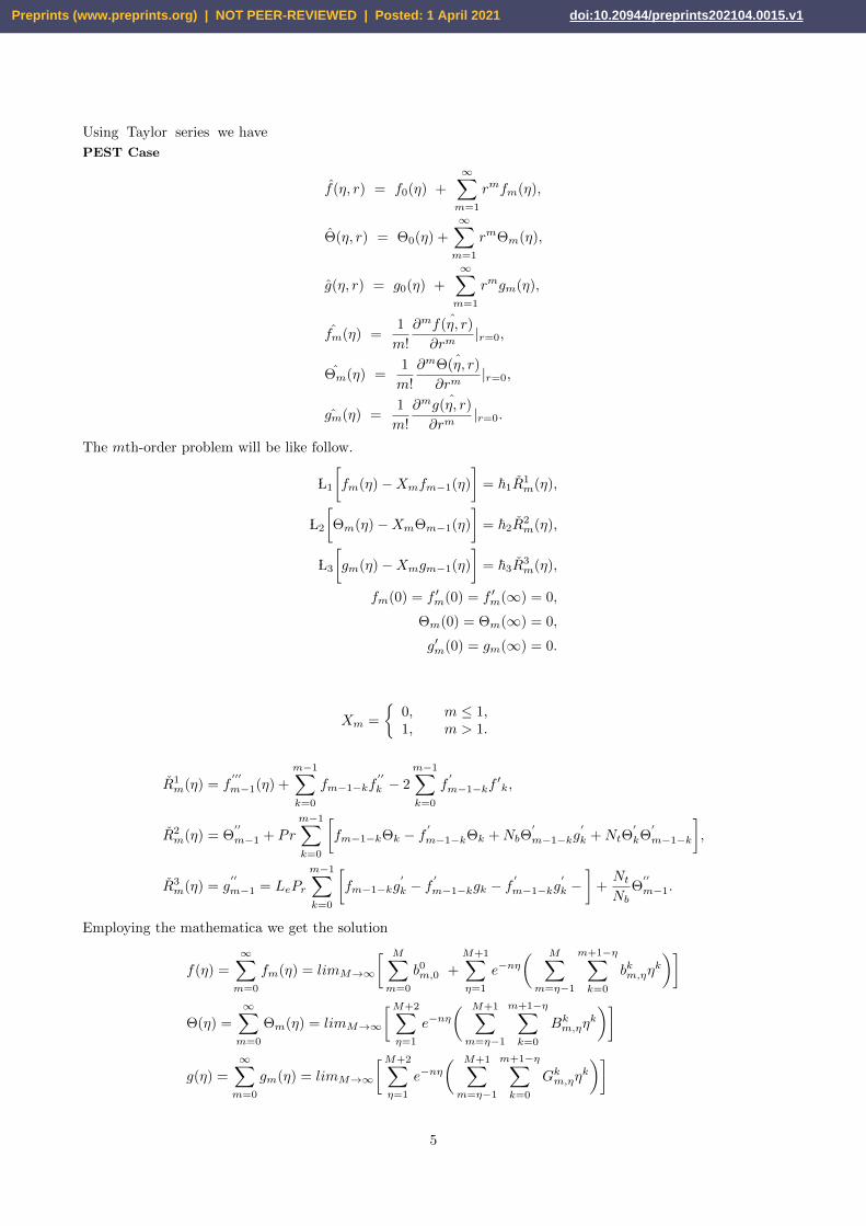
UsingpTaylorpseriespwe have

PEST Case

f(η, r) = f0(η) +

∞∑m=1

rmfm(η),

Θ(η, r) = Θ0(η) +

∞∑m=1

rmΘm(η),

g(η, r) = g0(η) +

∞∑m=1

rmgm(η),

fm(η) =1

m!

∂m ˆf(η, r)

∂rm|r=0,

Θm(η) =1

m!

∂m ˆΘ(η, r)

∂rm|r=0,

gm(η) =1

m!

∂m ˆg(η, r)

∂rm|r=0.

The mth-order problem will be like follow.

L1

[fm(η)−Xmfm−1(η)

]= ~1R

1m(η),

L2

[Θm(η)−XmΘm−1(η)

]= ~2R

2m(η),

L3

[gm(η)−Xmgm−1(η)

]= ~3R

3m(η),

fm(0) = f ′m(0) = f ′m(∞) = 0,

Θm(0) = Θm(∞) = 0,

g′m(0) = gm(∞) = 0.

Xm =

{0, m ≤ 1,1, m > 1.

R1m(η) = f

′′′

m−1(η) +

m−1∑k=0

fm−1−kf′′

k − 2

m−1∑k=0

f′

m−1−kf′k,

R2m(η) = Θ

′′

m−1 + Pr

m−1∑k=0

[fm−1−kΘk − f

′

m−1−kΘk +NbΘ′

m−1−kg′

k +NtΘ′

kΘ′

m−1−k

],

R3m(η) = g

′′

m−1 = LePr

m−1∑k=0

[fm−1−kg

′

k − f′

m−1−kgk − f′

m−1−kg′

k −]

+NtNb

Θ′′

m−1.

Employing the mathematica we get the solution

f(η) =

∞∑m=0

fm(η) = limM→∞

[ M∑m=0

b0m,0 +

M+1∑η=1

e−nη( M∑m=η−1

m+1−η∑k=0

bkm,ηηk

)]

Θ(η) =

∞∑m=0

Θm(η) = limM→∞

[M+2∑η=1

e−nη( M+1∑m=η−1

m+1−η∑k=0

Bkm,ηηk

)]

g(η) =

∞∑m=0

gm(η) = limM→∞

[M+2∑η=1

e−nη( M+1∑m=η−1

m+1−η∑k=0

Gkm,ηηk

)]

5



f (0)θ (0)

(

)

PEST Case

Nt = 0.5, Nb= 0.5, v= -0.1

Pr=1.5, Le=2.g(0)

-2.0 -1.5 -1.0 -0.5 0.0-3.0

-2.5

-2.0

-1.5

-1.0

-0.5

0.0

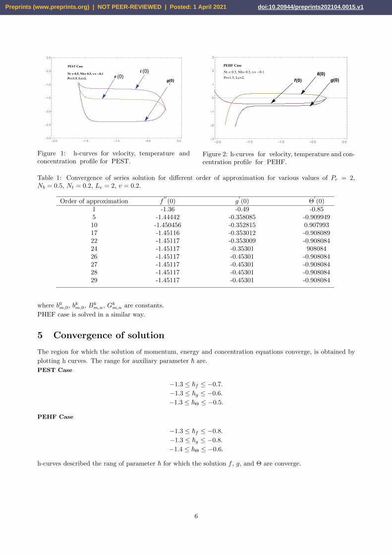
Figure 1: h-curvespforpvelocity,ptemperature andconcentrationpprofile forpPEST.

θ(0)f(0) g(0)

PEHF Case

Nt = 0.5, Nb= 0.5, v= -0.1

Pr=1.5, Le=2.

-2.0 -1.5 -1.0 -0.5 0.0-3

-2

-1

0

1

2

3

Figure 2: h-curvespforpvelocity, temperature and con-centration profilepforpPEHF.

Table 1: Convergence of series solution for different order of approximation for various values of Pr = 2,Nb = 0.5, Nt = 0.2, Le = 2, v = 0.2.

Order of approximation f′′(0) g

′(0) Θ

′(0)

1 -1.36 -0.49 -0.855 -1.44442 -0.358085 -0.90994910 -1.450456 -0.352815 0.90799317 -1.45116 -0.353012 -0.90808922 -1.45117 -0.353009 -0.90808424 -1.45117 -0.35301 90808426 -1.45117 -0.45301 -0.90808427 -1.45117 -0.45301 -0.90808428 -1.45117 -0.45301 -0.90808429 -1.45117 -0.45301 -0.908084

where b0m,0, bkm,0, Bkm,n, Gkm,n are constants.

PHEF case is solved in a similar way.

5 Convergence of solution

The region for which the solution of momentum, energy and concentration equations converge, is obtained by

plotting h curves. The range for auxiliary parameter ~ are.

PEST Case

−1.3 ≤ ~f ≤ −0.7.

−1.3 ≤ ~g ≤ −0.6.

−1.3 ≤ ~Θ ≤ −0.5.

PEHF Case

−1.3 ≤ ~f ≤ −0.8.

−1.3 ≤ ~g ≤ −0.8.

−1.4 ≤ ~Θ ≤ −0.6.

h-curves described the rang of parameter ~ for which the solution f , g, and Θ are converge.

6



Vw= -2

Vw=0.5

Vw=1

Vw=2

PEST Case

0 1 2 3 4 5 6 7

0.0

0.2

0.4

0.6

0.8

1.0

η

f'(η)

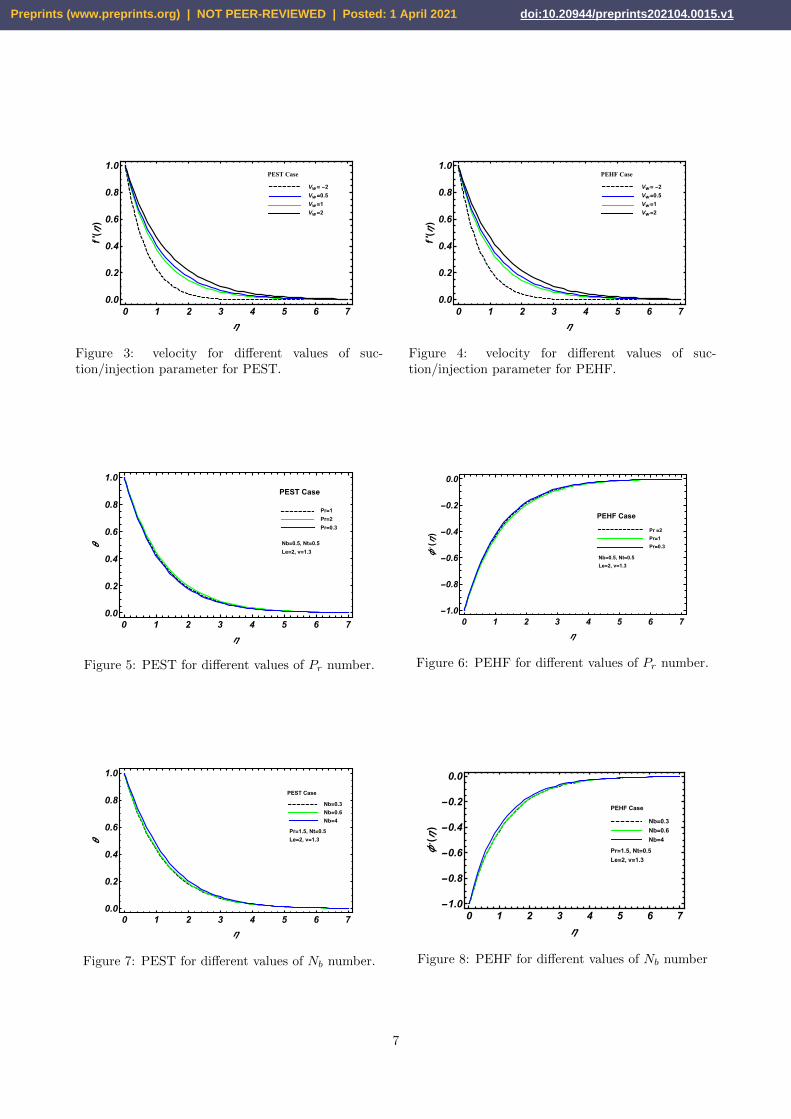
Figure 3: velocity for different values of suc-tion/injection parameter for PEST.

Vw= -2

Vw=0.5

Vw=1

Vw=2

PEHF Case

0 1 2 3 4 5 6 7

0.0

0.2

0.4

0.6

0.8

1.0

η

f'(η)

Figure 4: velocity for different values of suc-tion/injection parameter for PEHF.

Pr=1

Pr=2

Pr=0.3

Nb=0.5, Nt=0.5

Le=2, v=1.3

PEST Case

0 1 2 3 4 5 6 7

0.0

0.2

0.4

0.6

0.8

1.0

η

θ

Figure 5: PEST for different values of Pr number.

Pr =2

Pr=1

Pr=0.3

PEHF Case

Nb=0.5, Nt=0.5

Le=2, v=1.3

0 1 2 3 4 5 6 7

-1.0

-0.8

-0.6

-0.4

-0.2

0.0

η

ϕ, (η)

Figure 6: PEHF for different values of Pr number.

PEST Case

Nb=0.3

Nb=0.6

Nb=4

Pr=1.5, Nt=0.5

Le=2, v=1.3

0 1 2 3 4 5 6 7

0.0

0.2

0.4

0.6

0.8

1.0

η

θ

Figure 7: PEST for different values of Nb number.

Nb=0.3

Nb=0.6

Nb=4

PEHF Case

Pr=1.5, Nt=0.5

Le=2, v=1.3

0 1 2 3 4 5 6 7

-1.0

-0.8

-0.6

-0.4

-0.2

0.0

η

ϕ, (η)

Figure 8: PEHF for different values of Nb number

7



PEST Case

Le=1

Le=2

Le=50

Pr=1.5, Nt=0,

Nb=0.5, v=1.3

0 1 2 3 4 5 6 7

0.0

0.2

0.4

0.6

0.8

1.0

η

θ

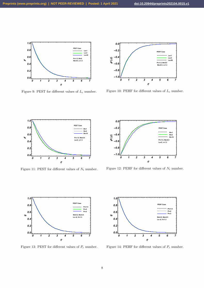
Figure 9: PEST for different values of Le number.

Le=1

Le=2

Le=50

PEHF Case

Pr=1.5, Nt=0.5

Nb=0.5, v=1.3

0 1 2 3 4 5 6 7

-1.0

-0.8

-0.6

-0.4

-0.2

0.0

η

ϕ, (η)

Figure 10: PEHF for different values of Le number.

PEST Case

Nt=1

Nt=2

Nt=10

Pr=1.5, Nb=0.5

Le=2, v=1.3

0 1 2 3 4 5 6 7

0.0

0.2

0.4

0.6

0.8

1.0

η

θ

Figure 11: PEST for different values of Nt number.

Nt=1

Nt=2

Nt=10

PEHF Case

Pr=1.5, Nb=0.5

Le=2, v=1.3

0 1 2 3 4 5 6 7

-1.0

-0.8

-0.6

-0.4

-0.2

0.0

η

ϕ, (η)

Figure 12: PEHF for different values of Nt number.

Pr=1.5

Pr=2

Pr=3

PEST Case

Nt=0.5, Nb=0.5

Le =2, V=1.3

0 1 2 3 4 5 6 70.0

0.2

0.4

0.6

0.8

1.0

η

g

Figure 13: PEST for different values of Pr number.

Pr=1.5

Pr=2

Pr=3

PEHF Case

Nt=0.5, Nb=0.5

Le =2, V=1.3

0 1 2 3 4 5 6 70.0

0.2

0.4

0.6

0.8

1.0

η

g

Figure 14: PEHF for different values of Pr number.

8



Nb=0.2

Nb=1.3

Nb=4

pr=1.5, Nt=0.5

Le=2, v=1.3

PEST Case

0 1 2 3 4 5 6 7

0.0

0.2

0.4

0.6

0.8

1.0

η

g

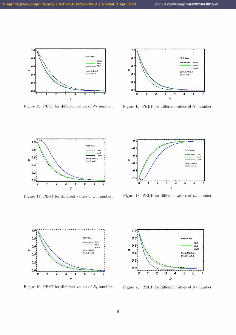
Figure 15: PEST for different values of Nb number.

Nb=0.2

Nb=1.3

Nb=4

pr=1.5, Nt=0.5

Le=2, v=1.3

PEHF Case

0 1 2 3 4 5 6 7

0.0

0.2

0.4

0.6

0.8

1.0

η

g

Figure 16: PEHF for different values of Nb number.

PEST Case

Le=2

Le=4

Le=20

Nt=0.5, Nb=0.5,

Pr=1.2, v=1.3

0 1 2 3 4 5 6 70.0

0.2

0.4

0.6

0.8

1.0

η

g

Figure 17: PEST for different values of Le number.

PEHF case:

Le=2

Le=4

Le=20

Nt=0.5, Nb=0.5,

Pr=1.2, v=1.3

0 1 2 3 4 5 6 7

-1.0

-0.8

-0.6

-0.4

-0.2

0.0

η

g

Figure 18: PEHF for different values of Le number.

PEST Case

Nt=1

Nt=3

Nt=10

Le=2, Nb=0.5,

Pr=1.2, v=1.3

0 1 2 3 4 5 6 70.0

0.2

0.4

0.6

0.8

1.0

η

g

Figure 19: PEST for different values of Nt number.

Nt=1

Nt=3

Nt=10

Le=2, Nb=0.5,

Pr=1.2, v=1.3

PEHF Case

0 1 2 3 4 5 6 7

0.0

0.2

0.4

0.6

0.8

1.0

η

g

Figure 20: PEHF for different values of Nt number.

9



6 Results and Discussion

The solution of the governing problem is executed with the help of Mathematica and the results are plotted

graphically, which characterizes the behavior of the problem. A comparison is made between the graphical results

of two distinct cases of the problem i.e. PEHF and PEST. Initially we have prepared the results of h-curves

for velocity, temperature and concentration profiles as plotted in figures 1 & 2. To deal with different flow

parameters we have first prepared the individual graphical results of velocity profile for the two different classes of

PEST and PEHF as shown in figures 3 & 4. These figures illustrate the effect of suction/injection parameter,

which is in direct relation to the velocity profile, i.e. when we increase the suction/injection parameter the

velocity profile also going to increase for both PEST and PEHF in the same manner. In the same way, the

temperature profiles are plotted for distinct values of the Prandtl number as found in figures 5 & 6. It is noticed

that with the escalation Pr, the temperature profile shoots up only for PEST case, whereas temperature decrease

in the case of PEHF.

In figures 7 & 8 the different values of Nb have shown their influence on the Θ(η). It appears that with the

escalation of Nb there is a boost in Θ(η) for both PEST as well as PEHF case and the boundary layer declines

for PEST, although it modifies for PEHF. Figures 9 & 10 indicates the Θ(η) profile for the different values

of Le which provides a very minimal change in Θ(η) for each case of PEST and PEHF. However, by making a

big change in Le there is a slight decrease in the Θ(η) for each case. For the various values of Nt, the separate

graphical results for the mutual case of PEST and PEHF can be detected respectively in figures 11 & 12. It

appears that the Θ(η) boosts with the escalation of Nt used for the PEST situation and for PEHF conditions

Θ(η) decreases.

The behavior of concentration profile forpdifferentpvalues of physical parameters Pr is respectively shown

in figures 13 & 14. These figures signify the change in nano-particles volume fraction which is caused by

making the change in Pr number. One can see that, for the joint conditions of PEST and PEHF, there is a

negligible change in g for different values of Pr as well as the same behavior is detected for the boundary layer.

Similarly, the concentration profile for several values of Nb is shown in figures 15 & 16. We have noted that

the escalation of Nb, induces a decrease in concentration profile g for PEST conditions, although g increases

for PEHF conditions. The effect of Le number on the nano-particles volume fractions is shown in figures 17

& 18. We see the same behavior for the joint conditions of PEST and PEHF, that is with the increase of Lenumber the concentration g individually shoots up for PEST as well as PEHF conditions. Figures 19 & 20.

represent the effect of Nt on g. It appears that with the escalation of Nt, there is an increase in g for PEHF

case whereas reduction is detected in case of PEST case.

7 Conclusion

• The velocity profile modifies for the enhancement of suction/injection parameter in both PEST and PEHF

case.

• The temperaturepprofilepmodifies for the enhancement of Pr only for PEST case, whereas it declines in

the case of PEHF.

• The escalation of Nb values causes to boost the temperaturepprofilepfor both PEST as well as PEHF case

while.

• The escalation of Nt values causes to improve both the temperature profile and concentration profile only

in case of PEST whereas a reduction is detected in case of PEST for both profiles.

• The escalation of Nb causes a decrease in concentration profile g for PEST case, although g increases for

PEHF case.

• The escalation of Le number causes to increase the nanoparticlespvolumepfractionpfor both PEST andpPEHF

case.

10



References

[1] Crane LJ. Flow past a stretching plate. Zeitschrift fur angewandte Mathematik und Physik ZAMP.

1970;21(4):645–647.

[2] Sakiadis BC. Boundary–layer behavior on continuous solid surfaces: II. The boundary layer on a contin-

uous flat surface. AiChE journal. 1961;7(2):221–225.

[3] Wang CY. Liquid film on an unsteady stretching surface. Quarterly of Applied Mathematics.

1990;48(4):601–610.

[4] Li X, Khan AU, Khan MR, Nadeem S, Khan SU. Oblique stagnation point flow of nanofluids over

stretching/shrinking sheet with Cattaneo–Christov heat flux model: existence of dual solution. Symmetry.

2019;11(9):1070.

[5] Khan MR. Numerical analysis of oblique stagnation point flow of nanofluid over a curved stretch-

ing/shrinking surface. Physica Scripta. 2020;9(10):105704.

[6] Nadeem S., Khan AU. MHD oblique stagnation point flow of nanofluid over an oscillatory stretch-

ing/shrinking sheet: Existence of dual solutions. Physica Scripta. 2019;94(7):075204.

[7] Nadeem S, Ullah N, Khan AU, Akbar T. Effect of homogeneous-heterogeneous reactions on ferrofluid in

the presence of magnetic dipole along a stretching cylinder. Results in physics. 2017;7:3574–3582.

[8] Sahoo B. Effects of slip, viscous dissipation and Joule heating on the MHD flow and heat transfer of a

second-grade fluid past a radially stretching sheet. Applied Mathematics and Mechanics (English Edition).

2010;31(2):159-173.

[9] Qaiser D, Zheng Z, Khan MR. Numerical assessment of mixed convection flow of Walters-B nanofluid

over a stretching surface with Newtonian heating and mass transfer. Thermal Science and Engineering

Progress. 2020;100801.

[10] Hayat T, Asad S, Alsaedi A. Flow of variable thermal conductivity fluid due to inclined stretching cylinder

with viscous dissipation and thermal radiation. Applied Mathematics and Mechanics (English Edition).

2014;35(6):717-728.

[11] Meqahid AM. Carreau fluid flow due to nonlinearly stretching sheet with thermal radiation, heat flux,

and variable conductivity. Applied Mathematics and Mechanics (English Edition). 2019;40(11):1615-1624.

[12] Zhu J, Zheng L, Zhang X. Second-order slip MHD flow and heat transfer of nanofluids with thermal

radiation and chemical reaction. Applied Mathematics and Mechanics (English Edition). 2015;36(9):1131-

1146.

[13] Mahanthesh B, Gireesha BJ, Shehzad SA, Abbasi FM, Gorla RS. Nonlinear three-dimensional stretched

flow of an Oldroyd-B fluid with convective condition, thermal radiation, and mixed convection. Applied

Mathematics and Mechanics (English Edition). 2017;38(7):969-980.

[14] Sheikhlesami M, Ellahi R. Three-dimensional mesoscopic simulation of magnetic field effect on natural

convection of nanofluid. International Journal of Heat and Mass Transfer. 2015;89:799–808.

[15] Haq RU., Khan ZH, Khan WA. Thermophysical effects of carbon nanotubes on MHD flow over a stretching

surface. Physica E: Low-dimensional Systems and Nanostructures. 2014;63:215–222.

[16] Mehmood R, Nadeem S, Massod S. Effects of transverse magnetic field on a rotating micropolar fluid

between parallel plates with heat transfer. Journal of Magnetism and Magnetic Materials. 2016;40:1006–

1014.

[17] Borrelli A, Giantesio G, Patria MC. MHD oblique stagnation-point flow of a Newtonian fluid. Zeitschrift

fur angewandte Mathematik und Physik. 2012;63(2):271–294.

[18] Nadeem S, Khan MR, Khan AU. MHD stagnation point flow of viscous nanofluid over a curved surface.

Physica Scripta. 2019;94(11):115207.

[19] Khan M, Malik R, Anjum A. Exact solutions of MHD second Stokes flow of generalized Burgers fluid.

Applied Mathematics and Mechanics (English Edition). 2015;36(2):211-224.

11



[20] Ali FM, Nazar R, Arifin NM, Pop I. MHD stagnation-point flow and heat transfer towards stretching sheet

with induced magnetic field. Applied Mathematics and Mechanics (English Edition). 2011;32(4):409-418.

[21] Zhu J, Zheng LC, Zhang ZG. Effects of slip condition on MHD stagnation-point flow over a power-law

stretching sheet. Applied Mathematics and Mechanics (English Edition). 2010;31(4):439-448.

[22] Rauf A, Abbas Z, Shehzad S A. Utilization of Maxwell-Cattaneo law for MHD swirling flow through

oscillatory disk subject to porous medium. Applied Mathematics and Mechanics (English Edition).

2019;40(6):837-850.

[23] Haq RU, Nadeem S, Khan ZH, Akbar NS. Thermal radiation and slip effects on MHD stagnation point flow

of nanofluid over a stretching sheet. Physica E: Low-dimensional systems and nanostructures. 2015;65:17-

23.

[24] Ramzan M, Chung JD, Ullah N. Partial slip effect in the flow of MHD micropolar nanofluid flow due to

a rotating disk–A numerical approach. Results in physics. 2017;7:3557–3566.

[25] Nadeem S, Akhtar S, Abbas N. Heat transfer of Maxwell base fluid flow of nanomaterial with MHD over

a vertical moving surface. Alexandria Engineering Journal. 2020.

[26] Uddin I, Ullah I, Ali R, Khan I, Nisar KS. Numerical analysis of nonlinear mixed convective MHD

chemically reacting flow of Prandtl—Eyring nanofluids in the presence of activation energy and Joule

heating. Journal of Thermal Analysis and Calormitory. 2020. https://doi.org/10.1007/s10973-020-09574-

2.

[27] Ullah I, Ali R, Khan I, Nisar KS. Insight into kerosene conveying SWCNT and MWCNT nanoparticles

through a porous medium: significance of Coriolis force and entropy generation. Physica Scripta. 2021;1:1–

11.

[28] Nadeem S, Hussain ST. Heat transfer analysis of Williamson fluid over exponentially stretching surface.

Applied Mathematics and Mechanics (English Edition). 2014;35(4):489-502.

[29] Nadeem S, Hussain ST, Lee C. Flow of a Williamson fluid over a stretching sheet. Brazilian journal of

chemical engineering. 2013;30(3):619-625.

12



mathematical analysis of heat and mass transfer for

Documents