mathematical foundations of automata theory
TRANSCRIPT

Mathematical Foundations
of Automata Theory
Jean-Eric Pin
Version of November 30, 2016

2
Preface
These notes form the core of a future book on the algebraic foundations ofautomata theory. This book is still incomplete, but the first eleven chaptersnow form a relatively coherent material, covering roughly the topics describedbelow.
The early years of automata theory
Kleene’s theorem [66] is usually considered as the starting point of automatatheory. It shows that the class of recognisable languages (that is, recognisedby finite automata), coincides with the class of rational languages, which aregiven by rational expressions. Rational expressions can be thought of as ageneralisation of polynomials involving three operations: union (which plays therole of addition), product and the star operation. It was quickly observed thatthese essentially combinatorial definitions can be interpreted in a very rich wayin algebraic and logical terms. Automata over infinite words were introducedby Buchi in the early 1960s to solve decidability questions in first-order andmonadic second-order logic of one successor. Investigating two-successor logic,Rabin was led to the concept of tree automata, which soon became a standardtool for studying logical definability.
The algebraic approach
The definition of the syntactic monoid, a monoid canonically attached to eachlanguage, was first given by Schutzenberger in 1956 [133]. It later appeared ina paper of Rabin and Scott [124], where the notion is credited to Myhill. Itwas shown in particular that a language is recognisable if and only if its syn-tactic monoid is finite. However, the first classification results on recognisablelanguages were rather stated in terms of automata [84] and the first nontrivialuse of the syntactic monoid is due to Schutzenberger [134]. Schutzenberger’stheorem (1965) states that a rational language is star-free if and only if its syn-tactic monoid is finite and aperiodic. This elegant result is considered, rightafter Kleene’s theorem, as the most important result of the algebraic theory ofautomata. Schutzenberger’s theorem was supplemented a few years later by aresult of McNaughton [80], which establishes a link between star-free languagesand first-order logic of the order relation.
Both results had a considerable influence on the theory. Two other importantalgebraic characterisations date back to the early seventies: Simon [137] provedthat a rational language is piecewise testable if and only if its syntactic monoidis J -trivial and Brzozowski-Simon [21] and independently, McNaughton [79]
3
4
characterised the locally testable languages. The logical counterpart of the firstresult was obtained by Thomas [158]. These successes settled the power of thealgebraic approach, which was axiomatized by Eilenberg in 1976 [40].
Eilenberg’s variety theory
A variety of finite monoids is a class of monoids closed under taking submonoids,quotients and finite direct products. Eilenberg’s theorem states that varieties offinite monoids are in one-to-one correspondence with certain classes of recognis-able languages, the varieties of languages. For instance, the rational languagesare associated with the variety of all finite monoids, the star-free languages withthe variety of finite aperiodic monoids, and the piecewise testable languages withthe variety of finite J -trivial monoids. Numerous similar results have been es-tablished over the past thirty years and, for this reason, the theory of finiteautomata is now intimately related to the theory of finite monoids.
Several attempts were made to extend Eilenberg’s variety theory to a largerscope. For instance, partial order on syntactic semigroups were introduced in[94], leading to the notion of ordered syntactic semigroups. The resulting exten-sion of Eilenberg’s variety theory permits one to treat classes of languages thatare not necessarily closed under complement, contrary to the original theory.Other extensions were developed independently by Straubing [153] and Esik andIto [43].
The topological point of view
Due allowance being made, the introduction of topology in automata theory canbe compared to the use of p-adic analysis in number theory.
The notion of a variety of finite monoids was coined after a similar notion,introduced much earlier by Birkhoff for infinite monoids: a Birkhoff variety ofmonoids is a class of monoids closed under taking submonoids, quotient monoidsand direct products. Birkhoff proved in [13] that his varieties can be defined bya set of identities: for instance the identity xy = yx characterises the varietyof commutative monoids. Almost fifty years later, Reiterman [126] extendedBirkhoff’s theorem to varieties of finite monoids: any variety of finite monoidscan be characterised by a set of profinite identities. A profinite identity is anidentity between two profinite words. Profinite words can be viewed as limitsof sequences of words for a certain metric, the profinite metric. For instance,one can show that the sequence xn! converges to a profinite word denoted byxω and the variety of finite aperiodic monoids can be defined by the identityxω = xω+1.
The profinite approach is not only a powerful tool for studying varieties butit also led to unexpected developments, which are at the heart of the currentresearch in this domain. In particular, Gehrke, Grigorieff and the author [45]proved that any lattice of recognisable languages can be defined by a set ofprofinite equations, a result that subsumes Eilenberg’s variety theorem.
The logical approach
We already mentioned Buchi’s, Rabin’s and McNaughton’s remarkable resultson the connexion between logic and finite automata. Buchi’s sequential calculus

5
is a logical language to express combinatorial properties of words in a naturalway. For instance, properties like “a word contains two consecutive occurrencesof a” or “a word of even length” can be expressed in this logic. However, severalparameters can be adjusted. Different fragments of logic can be considered:first-order, monadic second-order, Σn-formulas and a large variety of logicaland nonlogical symbols can be employed.
There is a remarkable connexion between first-order logic and the concate-nation product. The polynomial closure of a class of languages L is the set oflanguages that are sums of marked products of languages of L. By alternatingBoolean closure and polynomial closure, one obtains a natural hierarchy of lan-guages. The level 0 is the Boolean algebra {∅, A∗}. Next, for each n > 0, thelevel 2n+ 1 is the polynomial closure of the level 2n and the level 2n+ 2 is theBoolean closure of the level 2n + 1. A very nice result of Thomas [158] showsthat a recognisable language is of level 2n+ 1 in this hierarchy if and only if itis definable by a Σn+1-sentence of first-order logic in the signature {<, (a)a∈A},where a is a predicate giving the positions of the letter a.
There are known algebraic characterisations for the three first levels of thishierarchy. In particular, the second level is the class of piecewise testable lan-guages characterised by Simon [136].
Contents of these notes
The algebraic approach to automata theory relies mostly on semigroup theory,a branch of algebra which is usually not part of the standard background of astudent in mathematics or in computer science. For this reason, an importantpart of these notes is devoted to an introduction to semigroup theory. ChapterII gives the basic definitions and Chapter V presents the structure theory offinite semigroups. Chapters XIII and XV introduce some more advanced tools,the relational morphisms and the semidirect and wreath products.
Chapter III gives a brief overview on finite automata and recognisable lan-guages. It contains in particular a complete proof of Kleene’s theorem whichrelies on Glushkov’s algorithm in one direction and on linear equations in theopposite direction. For a comprehensive presentation of this theory I recom-mend the book of my colleague Jacques Sakarovitch [131]. The recent book ofOlivier Carton [25] also contains a nice presentation of the basic properties offinite automata. Recognisable and rational subsets of a monoid are presented inChapter IV. The notion of a syntactic monoid is the key notion of this chapter,where we also discuss the ordered case. The profinite topology is introducedin Chapter VI. We start with a short synopsis on general topology and metricspaces and then discuss the relationship between profinite topology and recog-nisable languages. Chapter VII is devoted to varieties of finite monoids and toReiterman’s theorem. It also contains a large collection of examples. Chap-ter VIII presents the equational characterisation of lattices of languages andEilenberg’s variety theorem. Examples of application of these two results aregathered in Chapter IX. Chapters X and XI present two major results, at thecore of the algebraic approach to automata theory: Schutzenberger’s and Si-mon’s theorem. The last five chapters are still under construction. ChapterXII is about polynomial closure, Chapter XIV presents another deep result ofSchutzenberger about unambiguous star-free languages and its logical counter-part. Chapter XVI gives a brief introduction to sequential functions and the
6
wreath product principle. Chapter XVIII presents some logical descriptions oflanguages and their algebraic characterisations.
Notation and terminology
The term regular set is frequently used in the literature but there is some con-fusion on its interpretation. In Ginzburg [49] and in Hopcroft, Motwani andUllman [60], a regular set is a set of words accepted by a finite automaton. InSalomaa [132], it is a set of words defined by a regular grammar and in Car-oll and Long [24], it is a set defined by a regular expression. This is no realproblem for languages, since, by Kleene’s theorem, these three definitions areequivalent. This is more problematic for monoids in which Kleene’s theoremdoes not hold. Another source of confusion is that the term regular has a well-established meaning in semigroup theory. For these reasons, I prefer to use theterms recognisable and rational.
I tried to keep some homogeneity in notation. Most of the time, I use Greekletters for functions, lower case letters for elements, capital letters for sets andcalligraphic letters for sets of sets. Thus I write: “let s be an element of asemigroup S and let P(S) be the set of subsets of S”. I write functions on theleft and transformations and actions on the right. In particular, I denote by q ·uthe action of a word u on a state q. Why so many computer scientists preferthe awful notation δ(q, u) is still a mystery. It leads to heavy formulas, likeδ(δ(q, u), v) = δ(q, uv), to be compared to the simple and intuitive (q ·u)· v =q ·uv, for absolutely no benefit.
I followed Eilenberg’s tradition to use boldface letters, like V, to denotevarieties of semigroups, and to use calligraphic letters, like V, for varieties oflanguages. However, I have adopted Almeida’s suggestion to have a differentnotation for operators on varieties, like EV, LV or PV.
I use the term morphism for homomorphism. Semigroups are usually de-noted by S or T , monoids by M or N , alphabets are A or B and letters by a,b, c, . . . but this notation is not frozen: I may also use A for semigroup and Sfor alphabet if needed! Following a tradition in combinatorics, |E| denotes thenumber of elements of a finite set. The notation |u| is also used for the lengthof a word u, but in practice, there is no risk of confusion between the two.
To avoid repetitions, I frequently use brackets as an equivalent to “respec-tively”, like in the following sentence : a semigroup [monoid, group] S is com-mutative if, for all x, y ∈ S, xy = yx.
Lemmas, propositions, theorems and corollaries share the same counter andare numbered by section. Examples have a separate counter, but are also num-bered by section. References are given according to the following example:Theorem 1.6, Corollary 1.5 and Section 1.2 refer to statements or sections ofthe same chapter. Proposition VI.3.12 refers to a proposition which is externalto the current chapter.
Acknowledgements
Several books on semigroups helped me in preparing these notes. Clifford andPreston’s treatise [28, 29] remains the classical reference. My favourite sourcefor the structure theory is Grillet’s remarkable presentation [53]. I also borroweda lot from the books by Almeida [3], Eilenberg [40], Higgins [58], Lallement [73]

7
and Lothaire [75] and also of course from my own books [91, 86]. Anothersource of inspiration (not yet fully explored!) are the research articles by mycolleagues Jorge Almeida, Karl Auinger, Jean-Camille Birget, Olivier Carton,Mai Gehrke, Victor Guba, Rostislav Horcık, John McCammond, Stuart W.Margolis, Dominique Perrin, Mark Sapir, Imre Simon, Ben Steinberg, HowardStraubing, Pascal Tesson, Denis Therien, Misha Volkov, Pascal Weil and MarcZeitoun.
I would like to thank my Ph.D. students Laure Daviaud, Luc Dartois,Charles Paperman and Yann Pequignot, my colleagues at LIAFA and LaBRIand the students of the Master Parisien de Recherches en Informatique (notablyAiswarya Cyriac, Nathanael Fijalkow, Agnes Kohler, Arthur Milchior, Anca Ni-tulescu, Pierre Pradic, Leo Stefanesco, Boker Udi, Jill-Jenn Vie and Furcy) forpointing out many misprints and corrections on earlier versions of this doc-ument. I would like to acknowledge the assistance and the encouragementsof my colleagues of the Picasso project, Adolfo Ballester-Bolinches, AntonioCano Gomez, Ramon Esteban-Romero, Xaro Soler-Escriva, Maria Belen SolerMonreal, Jorge Palanca and of the Pessoa project, Jorge Almeida, Mario J.J. Branco, Vıtor Hugo Fernandes, Gracinda M. S. Gomes and Pedro V. Silva.Other careful readers include Achim Blumensath and Martin Beaudry (with thehelp of his student Cedric Pinard) who proceeded to a very careful reading ofthe manuscript. George Hansoul, Sbastien Labb, Anne Schilling and HerbertToth sent me some very useful remarks. Special thanks are due to Jean Bersteland to Paul Gastin for providing me with their providential LATEX packages.
Paris, November 2016
Jean-Eric Pin

Contents
I Algebraic preliminaries . . . . . . . . . . . . . . . . . . . . . . . 1
1 Subsets, relations and functions . . . . . . . . . . . . . . . . . . . . 11.1 Sets . . . . . . . . . . . . . . . . . . . . . . . . . . . . . . . 11.2 Relations . . . . . . . . . . . . . . . . . . . . . . . . . . . . 11.3 Functions . . . . . . . . . . . . . . . . . . . . . . . . . . . . 21.4 Injective and surjective relations . . . . . . . . . . . . . . . 41.5 Relations and set operations . . . . . . . . . . . . . . . . . 7
2 Ordered sets . . . . . . . . . . . . . . . . . . . . . . . . . . . . . . . 83 Exercises . . . . . . . . . . . . . . . . . . . . . . . . . . . . . . . . . 9
II Semigroups and beyond . . . . . . . . . . . . . . . . . . . . . . 11
1 Semigroups, monoids and groups . . . . . . . . . . . . . . . . . . . 111.1 Semigroups, monoids . . . . . . . . . . . . . . . . . . . . . 111.2 Special elements . . . . . . . . . . . . . . . . . . . . . . . . 121.3 Groups . . . . . . . . . . . . . . . . . . . . . . . . . . . . . 131.4 Ordered semigroups and monoids . . . . . . . . . . . . . . 141.5 Semirings . . . . . . . . . . . . . . . . . . . . . . . . . . . . 14
2 Examples . . . . . . . . . . . . . . . . . . . . . . . . . . . . . . . . 152.1 Examples of semigroups . . . . . . . . . . . . . . . . . . . . 152.2 Examples of monoids . . . . . . . . . . . . . . . . . . . . . 162.3 Examples of groups . . . . . . . . . . . . . . . . . . . . . . 162.4 Examples of ordered monoids . . . . . . . . . . . . . . . . . 162.5 Examples of semirings . . . . . . . . . . . . . . . . . . . . . 16
3 Basic algebraic structures . . . . . . . . . . . . . . . . . . . . . . . 173.1 Morphisms . . . . . . . . . . . . . . . . . . . . . . . . . . . 173.2 Subsemigroups . . . . . . . . . . . . . . . . . . . . . . . . . 183.3 Quotients and divisions . . . . . . . . . . . . . . . . . . . . 193.4 Products . . . . . . . . . . . . . . . . . . . . . . . . . . . . 203.5 Ideals . . . . . . . . . . . . . . . . . . . . . . . . . . . . . . 203.6 Simple and 0-simple semigroups . . . . . . . . . . . . . . . 223.7 Semigroup congruences . . . . . . . . . . . . . . . . . . . . 22
4 Transformation semigroups . . . . . . . . . . . . . . . . . . . . . . 254.1 Definitions . . . . . . . . . . . . . . . . . . . . . . . . . . . 254.2 Full transformation semigroups and symmetric groups . . . 264.3 Product and division . . . . . . . . . . . . . . . . . . . . . 26
5 Generators . . . . . . . . . . . . . . . . . . . . . . . . . . . . . . . . 275.1 A-generated semigroups . . . . . . . . . . . . . . . . . . . . 27
i

ii CONTENTS
5.2 Cayley graphs . . . . . . . . . . . . . . . . . . . . . . . . . 285.3 Free semigroups . . . . . . . . . . . . . . . . . . . . . . . . 285.4 Universal properties . . . . . . . . . . . . . . . . . . . . . . 295.5 Presentations and rewriting systems . . . . . . . . . . . . . 29
6 Idempotents in finite semigroups . . . . . . . . . . . . . . . . . . . 307 Exercises . . . . . . . . . . . . . . . . . . . . . . . . . . . . . . . . . 33
III Languages and automata . . . . . . . . . . . . . . . . . . . . . 35
1 Words and languages . . . . . . . . . . . . . . . . . . . . . . . . . . 351.1 Words . . . . . . . . . . . . . . . . . . . . . . . . . . . . . . 351.2 Orders on words . . . . . . . . . . . . . . . . . . . . . . . . 361.3 Languages . . . . . . . . . . . . . . . . . . . . . . . . . . . 36
2 Rational languages . . . . . . . . . . . . . . . . . . . . . . . . . . . 383 Automata . . . . . . . . . . . . . . . . . . . . . . . . . . . . . . . . 40
3.1 Finite automata and recognisable languages . . . . . . . . . 403.2 Deterministic automata . . . . . . . . . . . . . . . . . . . . 433.3 Complete, accessible, coaccessible and trim automata . . . 453.4 Standard automata . . . . . . . . . . . . . . . . . . . . . . 46
4 Operations on recognisable languages . . . . . . . . . . . . . . . . . 464.1 Boolean operations . . . . . . . . . . . . . . . . . . . . . . 474.2 Product . . . . . . . . . . . . . . . . . . . . . . . . . . . . . 494.3 Star . . . . . . . . . . . . . . . . . . . . . . . . . . . . . . . 504.4 Quotients . . . . . . . . . . . . . . . . . . . . . . . . . . . . 524.5 Inverses of morphisms . . . . . . . . . . . . . . . . . . . . . 534.6 Minimal automata . . . . . . . . . . . . . . . . . . . . . . . 53
5 Rational versus recognisable . . . . . . . . . . . . . . . . . . . . . . 565.1 Local languages . . . . . . . . . . . . . . . . . . . . . . . . 565.2 Glushkov’s algorithm . . . . . . . . . . . . . . . . . . . . . 595.3 Linear equations . . . . . . . . . . . . . . . . . . . . . . . . 625.4 Extended automata . . . . . . . . . . . . . . . . . . . . . . 655.5 Kleene’s theorem . . . . . . . . . . . . . . . . . . . . . . . . 67
6 Exercises . . . . . . . . . . . . . . . . . . . . . . . . . . . . . . . . . 687 Notes . . . . . . . . . . . . . . . . . . . . . . . . . . . . . . . . . . . 71
IV Recognisable and rational sets . . . . . . . . . . . . . . . . . . 73
1 Rational subsets of a monoid . . . . . . . . . . . . . . . . . . . . . 732 Recognisable subsets of a monoid . . . . . . . . . . . . . . . . . . . 75
2.1 Recognition by monoid morphisms . . . . . . . . . . . . . . 752.2 Operations on sets . . . . . . . . . . . . . . . . . . . . . . . 772.3 Recognisable sets . . . . . . . . . . . . . . . . . . . . . . . . 78
3 Connexion with automata . . . . . . . . . . . . . . . . . . . . . . . 813.1 Transition monoid of a deterministic automaton . . . . . . 813.2 Transition monoid of a nondeterministic automaton . . . . 833.3 Monoids versus automata . . . . . . . . . . . . . . . . . . . 84
4 The syntactic monoid . . . . . . . . . . . . . . . . . . . . . . . . . . 864.1 Definitions . . . . . . . . . . . . . . . . . . . . . . . . . . . 864.2 The syntactic monoid of a language . . . . . . . . . . . . . 874.3 Computation of the syntactic monoid of a language . . . . 88
5 Recognition by ordered structures . . . . . . . . . . . . . . . . . . . 89

CONTENTS iii
5.1 Ordered automata . . . . . . . . . . . . . . . . . . . . . . . 895.2 Recognition by ordered monoids . . . . . . . . . . . . . . . 905.3 Syntactic order . . . . . . . . . . . . . . . . . . . . . . . . . 905.4 Computation of the syntactic ordered monoid . . . . . . . . 91
6 Exercises . . . . . . . . . . . . . . . . . . . . . . . . . . . . . . . . . 937 Notes . . . . . . . . . . . . . . . . . . . . . . . . . . . . . . . . . . . 94
V Green’s relations and local theory . . . . . . . . . . . . . . . . 95
1 Green’s relations . . . . . . . . . . . . . . . . . . . . . . . . . . . . 952 Inverses, weak inverses and regular elements . . . . . . . . . . . . . 103
2.1 Inverses and weak inverses . . . . . . . . . . . . . . . . . . 1032.2 Regular elements . . . . . . . . . . . . . . . . . . . . . . . . 105
3 Rees matrix semigroups . . . . . . . . . . . . . . . . . . . . . . . . 1074 Structure of regular D-classes . . . . . . . . . . . . . . . . . . . . . 112
4.1 Structure of the minimal ideal . . . . . . . . . . . . . . . . 1135 Green’s relations in subsemigroups and quotients . . . . . . . . . . 114
5.1 Green’s relations in subsemigroups . . . . . . . . . . . . . . 1145.2 Green’s relations in quotient semigroups . . . . . . . . . . . 115
6 Green’s relations and transformations . . . . . . . . . . . . . . . . . 1187 Summary: a complete example . . . . . . . . . . . . . . . . . . . . 1218 Exercises . . . . . . . . . . . . . . . . . . . . . . . . . . . . . . . . . 1239 Notes . . . . . . . . . . . . . . . . . . . . . . . . . . . . . . . . . . . 125
VI Profinite words . . . . . . . . . . . . . . . . . . . . . . . . . . . . 127
1 Topology . . . . . . . . . . . . . . . . . . . . . . . . . . . . . . . . . 1271.1 General topology . . . . . . . . . . . . . . . . . . . . . . . . 1271.2 Metric spaces . . . . . . . . . . . . . . . . . . . . . . . . . . 1281.3 Compact spaces . . . . . . . . . . . . . . . . . . . . . . . . 1291.4 Topological semigroups . . . . . . . . . . . . . . . . . . . . 130
2 Profinite topology . . . . . . . . . . . . . . . . . . . . . . . . . . . . 1302.1 The free profinite monoid . . . . . . . . . . . . . . . . . . . 1302.2 Universal property of the free profinite monoid . . . . . . . 1332.3 ω-terms . . . . . . . . . . . . . . . . . . . . . . . . . . . . . 134
3 Recognisable languages and clopen sets . . . . . . . . . . . . . . . . 1364 Exercises . . . . . . . . . . . . . . . . . . . . . . . . . . . . . . . . . 1395 Notes . . . . . . . . . . . . . . . . . . . . . . . . . . . . . . . . . . . 139
VII Varieties . . . . . . . . . . . . . . . . . . . . . . . . . . . . . . . . 141
1 Varieties . . . . . . . . . . . . . . . . . . . . . . . . . . . . . . . . . 1412 Free pro-V monoids . . . . . . . . . . . . . . . . . . . . . . . . . . 1423 Identities . . . . . . . . . . . . . . . . . . . . . . . . . . . . . . . . . 145
3.1 What is an identity? . . . . . . . . . . . . . . . . . . . . . . 1453.2 Properties of identities . . . . . . . . . . . . . . . . . . . . 1463.3 Reiterman’s theorem . . . . . . . . . . . . . . . . . . . . . . 146
4 Examples of varieties . . . . . . . . . . . . . . . . . . . . . . . . . . 1484.1 Varieties of semigroups . . . . . . . . . . . . . . . . . . . . 1484.2 Varieties of monoids . . . . . . . . . . . . . . . . . . . . . . 1524.3 Varieties of ordered monoids . . . . . . . . . . . . . . . . . 1574.4 Summary . . . . . . . . . . . . . . . . . . . . . . . . . . . . 157

iv CONTENTS
5 Exercises . . . . . . . . . . . . . . . . . . . . . . . . . . . . . . . . . 158
6 Notes . . . . . . . . . . . . . . . . . . . . . . . . . . . . . . . . . . . 160
VIII Equations and languages . . . . . . . . . . . . . . . . . . . . . . 161
1 Equations . . . . . . . . . . . . . . . . . . . . . . . . . . . . . . . . 161
2 Equational characterisation of lattices . . . . . . . . . . . . . . . . 162
3 Lattices of languages closed under quotients . . . . . . . . . . . . . 164
4 Streams of languages . . . . . . . . . . . . . . . . . . . . . . . . . . 165
5 C-streams . . . . . . . . . . . . . . . . . . . . . . . . . . . . . . . . 167
6 Varieties of languages . . . . . . . . . . . . . . . . . . . . . . . . . . 167
7 The variety theorem . . . . . . . . . . . . . . . . . . . . . . . . . . 168
8 Summary . . . . . . . . . . . . . . . . . . . . . . . . . . . . . . . . 172
9 Exercises . . . . . . . . . . . . . . . . . . . . . . . . . . . . . . . . . 172
10 Notes . . . . . . . . . . . . . . . . . . . . . . . . . . . . . . . . . . . 172
IX Algebraic characterisations . . . . . . . . . . . . . . . . . . . . 175
1 Varieties of languages . . . . . . . . . . . . . . . . . . . . . . . . . . 175
1.1 Locally finite varieties of languages . . . . . . . . . . . . . . 175
1.2 Commutative languages . . . . . . . . . . . . . . . . . . . . 178
1.3 R-trivial and L-trivial languages . . . . . . . . . . . . . . . 180
1.4 Some examples of +-varieties . . . . . . . . . . . . . . . . . 182
2 Lattices of languages . . . . . . . . . . . . . . . . . . . . . . . . . . 184
2.1 The role of the zero . . . . . . . . . . . . . . . . . . . . . . 185
2.2 Languages defined by density . . . . . . . . . . . . . . . . . 187
2.3 Cyclic and strongly cyclic languages . . . . . . . . . . . . . 193
3 Exercises . . . . . . . . . . . . . . . . . . . . . . . . . . . . . . . . . 199
4 Notes . . . . . . . . . . . . . . . . . . . . . . . . . . . . . . . . . . . 199
X Star-free languages . . . . . . . . . . . . . . . . . . . . . . . . . 201
1 Star-free languages . . . . . . . . . . . . . . . . . . . . . . . . . . . 201
2 Schutzenberger’s theorem . . . . . . . . . . . . . . . . . . . . . . . 202
3 Exercises . . . . . . . . . . . . . . . . . . . . . . . . . . . . . . . . . 206
4 Notes . . . . . . . . . . . . . . . . . . . . . . . . . . . . . . . . . . . 207
XI Piecewise testable languages . . . . . . . . . . . . . . . . . . . 209
1 Subword ordering . . . . . . . . . . . . . . . . . . . . . . . . . . . . 209
2 Simple languages and shuffle ideals . . . . . . . . . . . . . . . . . . 213
3 Piecewise testable languages and Simon’s theorem . . . . . . . . . . 214
4 Some consequences of Simon’s theorem . . . . . . . . . . . . . . . . 216
5 Exercises . . . . . . . . . . . . . . . . . . . . . . . . . . . . . . . . . 218
6 Notes . . . . . . . . . . . . . . . . . . . . . . . . . . . . . . . . . . . 219
XII Polynomial closure . . . . . . . . . . . . . . . . . . . . . . . . . 221
1 Polynomial closure of a lattice of languages . . . . . . . . . . . . . 221
2 A case study . . . . . . . . . . . . . . . . . . . . . . . . . . . . . . . 226
CONTENTS v
XIII Relational morphisms . . . . . . . . . . . . . . . . . . . . . . . . 227
1 Relational morphisms . . . . . . . . . . . . . . . . . . . . . . . . . . 2272 Injective relational morphisms . . . . . . . . . . . . . . . . . . . . . 2293 Relational V-morphisms . . . . . . . . . . . . . . . . . . . . . . . . 230
3.1 Aperiodic relational morphisms . . . . . . . . . . . . . . . . 2323.2 Locally trivial relational morphisms . . . . . . . . . . . . . 2323.3 Relational Jese 6 eK-morphisms . . . . . . . . . . . . . . . 233
4 Four examples of V-morphisms . . . . . . . . . . . . . . . . . . . . 2345 Mal’cev products . . . . . . . . . . . . . . . . . . . . . . . . . . . . 2356 Three examples of relational morphisms . . . . . . . . . . . . . . . 235
6.1 Concatenation product . . . . . . . . . . . . . . . . . . . . 2356.2 Pure languages . . . . . . . . . . . . . . . . . . . . . . . . . 2386.3 Flower automata . . . . . . . . . . . . . . . . . . . . . . . . 239
XIV Unambiguous star-free languages . . . . . . . . . . . . . . . . 241
1 Unambiguous star-free languages . . . . . . . . . . . . . . . . . . . 241
XV Wreath product . . . . . . . . . . . . . . . . . . . . . . . . . . . 243
1 Semidirect product . . . . . . . . . . . . . . . . . . . . . . . . . . . 2432 Wreath product . . . . . . . . . . . . . . . . . . . . . . . . . . . . . 2433 Basic decomposition results . . . . . . . . . . . . . . . . . . . . . . 2454 Exercises . . . . . . . . . . . . . . . . . . . . . . . . . . . . . . . . . 250
XVI Sequential functions . . . . . . . . . . . . . . . . . . . . . . . . . 251
1 Definitions . . . . . . . . . . . . . . . . . . . . . . . . . . . . . . . . 2511.1 Pure sequential transducers . . . . . . . . . . . . . . . . . . 2511.2 Sequential transducers . . . . . . . . . . . . . . . . . . . . . 254
2 Composition of sequential functions . . . . . . . . . . . . . . . . . . 2553 Sequential functions and wreath product . . . . . . . . . . . . . . . 2594 The wreath product principle and its consequences . . . . . . . . . 260
4.1 The wreath product principle . . . . . . . . . . . . . . . . . 2605 Applications of the wreath product principle . . . . . . . . . . . . . 261
5.1 The operations T 7→ U1 ◦ T and L 7→ LaA∗ . . . . . . . . . 2615.2 The operations T 7→ 2 ◦ T and L 7→ La . . . . . . . . . . . 2635.3 The operation T 7→ U2 ◦ T and star-free expressions . . . . 264
6 Exercises . . . . . . . . . . . . . . . . . . . . . . . . . . . . . . . . . 265
XVII Concatenation hierarchies . . . . . . . . . . . . . . . . . . . . . 267
1 Concatenation hierarchies . . . . . . . . . . . . . . . . . . . . . . . 267
XVIIIAn excursion into logic . . . . . . . . . . . . . . . . . . . . . . . 269
1 Introduction . . . . . . . . . . . . . . . . . . . . . . . . . . . . . . . 2692 The formalism of logic . . . . . . . . . . . . . . . . . . . . . . . . . 269
2.1 Syntax . . . . . . . . . . . . . . . . . . . . . . . . . . . . . 2692.2 Semantics . . . . . . . . . . . . . . . . . . . . . . . . . . . . 2722.3 Logic on words . . . . . . . . . . . . . . . . . . . . . . . . . 276
3 Monadic second-order logic on words . . . . . . . . . . . . . . . . . 2784 First-order logic of the linear order . . . . . . . . . . . . . . . . . . 281
vi CONTENTS
4.1 First order and star-free sets . . . . . . . . . . . . . . . . . 2824.2 Logical hierarchy . . . . . . . . . . . . . . . . . . . . . . . . 283
Annex 289
A A transformation semigroup . . . . . . . . . . . . . . . . . . . 291
References . . . . . . . . . . . . . . . . . . . . . . . . . . . . . . . . . . . 295
Index . . . . . . . . . . . . . . . . . . . . . . . . . . . . . . . . . . . . . . 307

Chapter I
Algebraic preliminaries
1 Subsets, relations and functions
1.1 Sets
The set of subsets of a set E is denoted by P(E) (or sometimes 2E). Thepositive Boolean operations on P(E) comprise union and intersection. TheBoolean operations also include complementation. The complement of a subsetX of E is denoted by Xc. Thus, for all subsets X and Y of E, the followingrelations hold
(Xc)c = X (X ∪ Y )c = Xc ∩ Y c (X ∩ Y )c = Xc ∪ Y c
We let |E| denote the number of elements of a finite set E, also called the sizeof E. A singleton is a set of size 1. We shall frequently identify a singleton {s}with its unique element s.
Given two sets E and F , the set of ordered pairs (x, y) such that x ∈ E andy ∈ F is written E × F and called the product of E and F .
1.2 Relations
Let E and F be two sets. A relation on E and F is a subset of E × F . IfE = F , it is simply called a relation on E. A relation τ can also be viewed asa function1 from E to P(F ) by setting, for each x ∈ E,
τ(x) = {y ∈ F | (x, y) ∈ τ}
By abuse of language, we say that τ is a relation from E into F .The inverse of a relation τ ⊆ E × F is the relation τ−1 ⊆ F ×E defined by
τ−1 = {(y, x) ∈ F × E | (x, y) ∈ τ}
Note that if τ is a relation from E in F , the relation τ−1 can be also viewed asa function from F into P(E) defined by
τ−1(y) = {x ∈ E | y ∈ τ(x)}
1Functions are formally defined in the next section, but we assume the reader is already
familiar with this notion.
1
2 CHAPTER I. ALGEBRAIC PRELIMINARIES
A relation from E into F can be extended to a function from P(E) into P(F )by setting, for each subset X of E,
τ(X) =⋃
x∈X
τ(x) = {y ∈ F | for some x ∈ X, (x, y) ∈ τ}
If Y is a subset of F , we then have
τ−1(Y ) =⋃
y∈Y
τ−1(y) = {x ∈ E | there exists y ∈ Y such that y ∈ τ(x)}
= {x ∈ E | τ(x) ∩ Y 6= ∅}
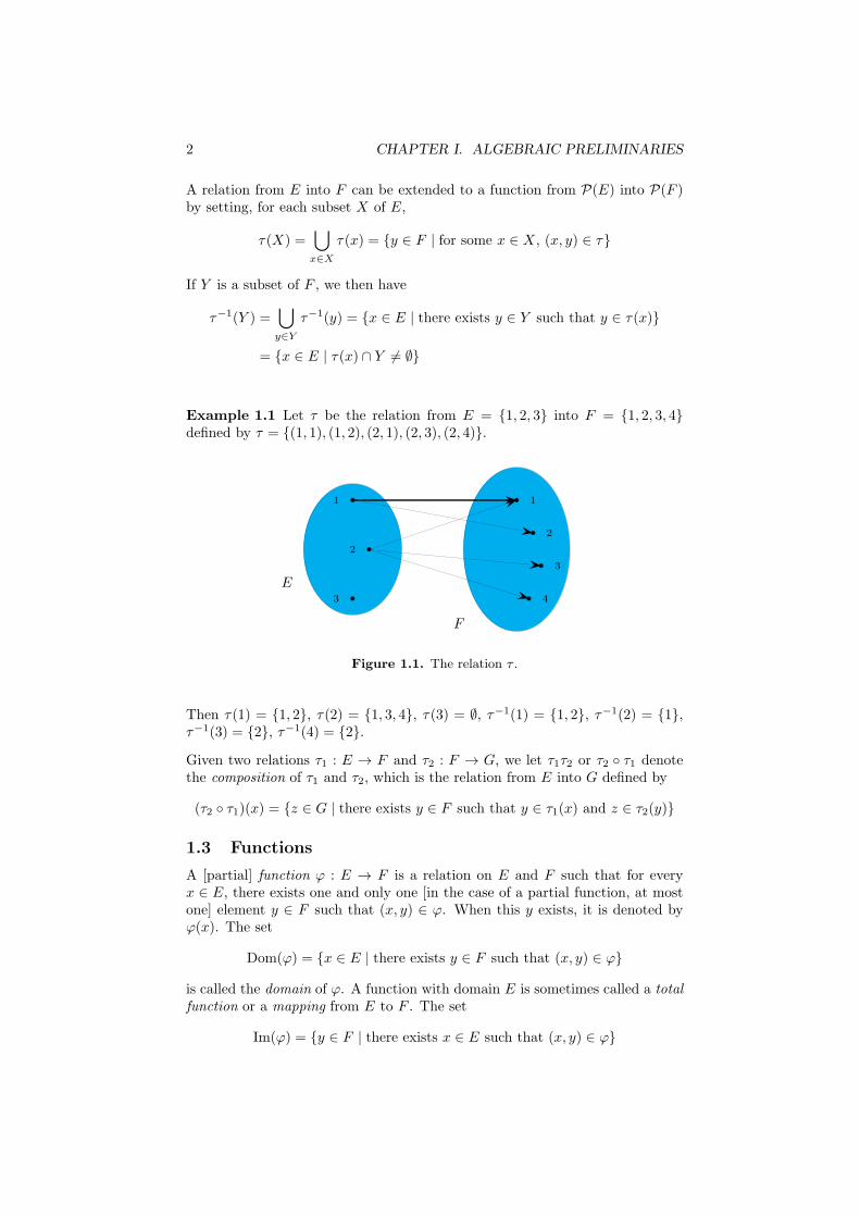
Example 1.1 Let τ be the relation from E = {1, 2, 3} into F = {1, 2, 3, 4}defined by τ = {(1, 1), (1, 2), (2, 1), (2, 3), (2, 4)}.
E
1
2
3
F
1
2
3
4
Figure 1.1. The relation τ .
Then τ(1) = {1, 2}, τ(2) = {1, 3, 4}, τ(3) = ∅, τ−1(1) = {1, 2}, τ−1(2) = {1},τ−1(3) = {2}, τ−1(4) = {2}.
Given two relations τ1 : E → F and τ2 : F → G, we let τ1τ2 or τ2 ◦ τ1 denotethe composition of τ1 and τ2, which is the relation from E into G defined by
(τ2 ◦ τ1)(x) = {z ∈ G | there exists y ∈ F such that y ∈ τ1(x) and z ∈ τ2(y)}
1.3 Functions
A [partial] function ϕ : E → F is a relation on E and F such that for everyx ∈ E, there exists one and only one [in the case of a partial function, at mostone] element y ∈ F such that (x, y) ∈ ϕ. When this y exists, it is denoted byϕ(x). The set
Dom(ϕ) = {x ∈ E | there exists y ∈ F such that (x, y) ∈ ϕ}
is called the domain of ϕ. A function with domain E is sometimes called a totalfunction or a mapping from E to F . The set
Im(ϕ) = {y ∈ F | there exists x ∈ E such that (x, y) ∈ ϕ}

1. SUBSETS, RELATIONS AND FUNCTIONS 3
is called the range or the image of ϕ. Given a set E, the identity mapping onE is the mapping IdE : E → E defined by IdE(x) = x for all x ∈ E.
A mapping ϕ : E → F is called injective if, for every u, v ∈ E, ϕ(u) = ϕ(v)implies u = v. It is surjective if, for every v ∈ F , there exists u ∈ E suchthat v ∈ ϕ(u). It is bijective if it is simultaneously injective and surjective. Forinstance, the identity mapping IdE(x) is bijective.
Proposition 1.1 Let ϕ : E → F be a mapping. Then ϕ is surjective if andonly if there exists a mapping ψ : F → E such that ϕ ◦ ψ = IdF .
Proof. If there exists a mapping ψ with these properties, we have ϕ(ψ(y)) = yfor all y ∈ F and thus ϕ is surjective. Conversely, suppose that ϕ is surjective.For each element y ∈ F , select an element ψ(y) in the nonempty set ϕ−1(y).This defines a mapping ψ : F → E such that ϕ ◦ ψ(y) = y for all y ∈ F .
A consequence of Proposition 1.1 is that surjective maps are right cancellative(the definition of a right cancellative map is transparent, but if needed, a formaldefinition is given in Section II.1.2).
Corollary 1.2 Let ϕ : E → F be a surjective mapping and let α and β be twomappings from F into G. If α ◦ ϕ = β ◦ ϕ, then α = β.
Proof. By Proposition 1.1, there exists a mapping ψ : F → E such that ϕ◦ψ =IdF . Therefore α ◦ ϕ = β ◦ ϕ implies α ◦ ϕ ◦ ψ = β ◦ ϕ ◦ ψ, whence α = β.
Proposition 1.3 Let ϕ : E → F be a mapping. Then ϕ is injective if and onlyif there exists a mapping ψ : Im(ϕ)→ E such that ψ ◦ ϕ = IdE.
Proof. Suppose there exists a mapping ψ with these properties. Then ϕ isinjective since the condition ϕ(x) = ϕ(y) implies ψ ◦ ϕ(x) = ψ ◦ ϕ(y), that is,x = y. Conversely, suppose that ϕ is injective. Define a mapping ψ : Im(ϕ)→ Eby setting ψ(y) = x, where x is the unique element of E such that ϕ(x) = y.Then ψ ◦ ϕ = IdE by construction.
It follows that injective maps are left cancellative.
Corollary 1.4 Let ϕ : F → G be an injective mapping and let α and β be twomappings from E into F . If ϕ ◦ α = ϕ ◦ β, then α = β.
Proof. By Proposition 1.3, there exists a mapping ψ : Im(ϕ) → F such thatψ◦ϕ = IdF . Therefore ϕ◦α = ϕ◦β implies ψ◦ϕ◦α = ψ◦ϕ◦β, whence α = β.
We come to a standard property of bijective maps.
Proposition 1.5 If ϕ : E → F is a bijective mapping, there exists a uniquebijective mapping from F to E, denoted by ϕ−1, such that ϕ ◦ ϕ−1 = IdF andϕ−1 ◦ ϕ = IdE.
4 CHAPTER I. ALGEBRAIC PRELIMINARIES
Proof. Since ϕ is bijective, for each y ∈ F there exists a unique x ∈ E suchthat ϕ(x) = y. Thus the condition ϕ−1◦ϕ = IdE requires that x = ϕ−1(ϕ(x)) =ϕ−1(y). This ensures the uniqueness of the solution. Now, the mapping ϕ−1 :F → E defined by ϕ−1(y) = x, where x is the unique element such that ϕ(x) =y, clearly satisfies the two conditions ϕ ◦ ϕ−1 = IdF and ϕ−1 ◦ ϕ = IdE .
The mapping ϕ−1 is called the inverse of ϕ.It is clear that the composition of two injective [surjective] mappings is injec-
tive [surjective]. A partial converse to this result is given in the next proposition.
Proposition 1.6 Let α : E → F and β : F → G be two mappings and letγ = β ◦ α be their composition.
(1) If γ is injective, then α is injective. If furthermore α is surjective, then βis injective.
(2) If γ is surjective, then β is surjective. If furthermore β is injective, thenα is surjective.
Proof. (1) Suppose that γ is injective. If α(x) = α(y), then β(α(x)) = β(α(y)),whence γ(x) = γ(y) and x = y since γ is injective. Thus α is injective. If,furthermore, α is surjective, then it is bijective and, by Proposition 1.5, γ◦α−1 =β ◦ α ◦ α−1 = β. It follows that β is the composition of the two injective mapsγ and α−1 and hence is injective.
(2) Suppose that γ is surjective. Then for each z ∈ G, there exists x ∈ Esuch that γ(x) = z. It follows that z = β(α(x)) and thus β is surjective. If,furthermore, β is injective, then it is bijective and, by Proposition 1.5, β−1 ◦γ =β−1 ◦ β ◦α = α. It follows that α is the composition of the two surjective mapsβ−1 and γ and hence is surjective.
The next result is extremely useful.
Proposition 1.7 Let E and F be two finite sets such that |E| = |F | and letϕ : E → F be a function. The following conditions are equivalent:
(1) ϕ is injective,
(2) ϕ is surjective,
(3) ϕ is bijective.
Proof. Clearly it suffices to show that (1) and (2) are equivalent. If ϕ is injec-tive, then ϕ induces a bijection from E onto ϕ(E). Thus |E| = |ϕ(E)| 6 |F | =|E|, whence |ϕ(E)| = |F | and ϕ(E) = F since F is finite.
Conversely, suppose that ϕ is surjective. By Proposition 1.1, there exists amapping ψ : F → E such that ϕ ◦ ψ = IdF . Since ψ is injective by Proposition1.6, and since we have already proved that (1) implies (2), ψ is surjective. Itfollows by Proposition 1.6 that ϕ is injective.
1.4 Injective and surjective relations
The notions of surjective and injective functions can be extended to relations asfollows. A relation τ : E → F is surjective if, for every v ∈ F , there exists u ∈ Esuch that v ∈ τ(u). It is called injective if, for every u, v ∈ E, τ(u) ∩ τ(v) 6= ∅implies u = v. The next three propositions provide equivalent definitions.
1. SUBSETS, RELATIONS AND FUNCTIONS 5
Proposition 1.8 A relation is injective if and only if its inverse is a partialfunction.
Proof. Let τ : E → F be a relation. Suppose that τ is injective. If y1, y2 ∈τ−1(x), then x ∈ τ(y1) ∩ τ(y2) and thus y1 = y2 since τ is injective. Thus τ−1
is a partial function.Suppose now that τ−1 is a partial function. If τ(x) ∩ τ(y) 6= ∅, there exists
some element c in τ(x)∩τ(y). It follows that x, y ∈ τ−1(c) and thus x = y sinceτ−1 is a partial function.
Proposition 1.9 Let τ : E → F be a relation. Then τ is injective if and onlyif, for all X,Y ⊆ E, X ∩ Y = ∅ implies τ(X) ∩ τ(Y ) = ∅.
Proof. Suppose that τ is injective and let X and Y be two disjoint subsets ofE. If τ(X) ∩ τ(Y ) 6= ∅, then τ(x) ∩ τ(y) 6= ∅ for some x ∈ X and y ∈ Y . Sinceτ is injective, it follows that x = y and hence X ∩ Y 6= ∅, a contradiction. ThusX ∩ Y = ∅.
If the condition of the statement holds, then it can be applied in particularwhen X and Y are singletons, say X = {x} and Y = {y}. Then the conditionbecomes x 6= y implies τ(x) ∩ τ(y) = ∅, that is, τ is injective.
Proposition 1.10 Let τ : E → F be a relation. The following conditions areequivalent:
(1) τ is injective,
(2) τ−1 ◦ τ = IdDom(τ),
(3) τ−1 ◦ τ ⊆ IdE.
Proof. (1) implies (2). Suppose that τ is injective and let y ∈ τ−1 ◦ τ(x). Bydefinition, there exists z ∈ τ(x) such that y ∈ τ−1(z). Thus x ∈ Dom(τ) andz ∈ τ(y). Now, τ(x) ∩ τ(y) 6= ∅ and since τ is injective, x = y. Thereforeτ−1 ◦ τ ⊆ IdDom(τ). But if x ∈ Dom(τ), there exists by definition y ∈ τ(x) andthus x ∈ τ−1 ◦ τ(x). Thus τ−1 ◦ τ = IdDom(τ).(2) implies (3) is trivial.(3) implies (1). Suppose that τ−1 ◦ τ ⊆ IdE and let x, y ∈ E. If τ(x) ∩ τ(y)contains an element z, then z ∈ τ(x), z ∈ τ(y) and y ∈ τ−1(z), whence y ∈τ−1 ◦ τ(x). Since τ−1 ◦ τ ⊆ IdE , it follows that y = x and thus τ is injective.
Proposition 1.10 has two useful consequences.
Corollary 1.11 Let τ : E → F be a relation. The following conditions areequivalent:
(1) τ is a partial function,
(2) τ ◦ τ−1 = IdIm(τ),
(3) τ ◦ τ−1 ⊆ IdF .
Proof. The result follows from Proposition 1.10 since, by Proposition 1.8, τ isa partial function if and only if τ−1 is injective.

6 CHAPTER I. ALGEBRAIC PRELIMINARIES
Corollary 1.12 Let τ : E → F be a relation. Then τ is a surjective partialfunction if and only if τ ◦ τ−1 = IdF .
Proof. Suppose that τ is a surjective partial function. Then by Corollary 1.11,τ ◦ τ−1 = IdF .
Conversely, if τ ◦ τ−1 = IdF , then τ is a partial function by Corollary 1.11and τ ◦ τ−1 = IdIm(τ). Therefore Im(τ) = F and τ is surjective.
Corollary 1.12 is often used in the following form.
Corollary 1.13 Let α : F → G and β : E → F be two functions and letγ = α ◦ β. If β is surjective, the relation γ ◦ β−1 is equal to α.
Proof. Indeed, γ = α ◦ β implies γ ◦ β−1 = α ◦ β ◦ β−1. Now, by Corollary1.12, β ◦ β−1 = IdF . Thus γ ◦ β−1 = α.
It is clear that the composition of two injective [surjective] relations is injec-tive [surjective]. Proposition 1.6 can also be partially adapted to relations.
Proposition 1.14 Let α : E → F and β : F → G be two relations and letγ = β ◦ α be their composition.
(1) If γ is injective and β−1 is surjective, then α is injective. If furthermoreα is a surjective partial function, then β is injective.
(2) If γ is surjective, then β is surjective. If furthermore β is injective ofdomain F , then α is surjective.
Proof. (1) Suppose that γ is injective. If α(x) ∩ α(y) 6= ∅, there exists anelement z ∈ α(x)∩α(y). Since β−1 is surjective, there is a t such that z ∈ β−1(t)or, equivalently, t ∈ β(z). Then t ∈ β(α(x))∩ β(α(y)), whence γ(x) = γ(y) andx = y since γ is injective. Thus α is injective.
If furthermore α is a surjective partial function, then by Proposition 1.8,α−1 is an injective relation and by Corollary 1.12, α ◦ α−1 = IdF . It followsthat γ ◦ α−1 = β ◦ α ◦ α−1 = β. Thus β is the composition of the two injectiverelations γ and α−1 and hence is injective.
(2) Suppose that γ is surjective. Then for each z ∈ G, there exists x ∈ Esuch that z ∈ γ(x). Thus there exists y ∈ α(x) such that z ∈ β(y), which showsthat β is surjective.
Suppose that β is injective of domain F or, equivalently, that β−1 is asurjective partial map. Then by Proposition 1.10, β−1 ◦β = IdF . It follows thatβ−1 ◦ γ = β−1 ◦ β ◦ α = α. Therefore α is the composition of the two surjectiverelations β−1 and γ and hence is surjective.
Proposition 1.15 Let E,F,G be three sets and α : G → E and β : G → Fbe two functions. Suppose that α is surjective and that, for every s, t ∈ G,α(s) = α(t) implies β(s) = β(t). Then the relation β ◦ α−1 : E → F is afunction.
Proof. Let x ∈ E. Since α is surjective, there exists y ∈ G such that α(y) = x.Setting z = β(y), one has z ∈ β ◦ α−1(x).
1. SUBSETS, RELATIONS AND FUNCTIONS 7
E F
G
α
β ◦ α−1
β
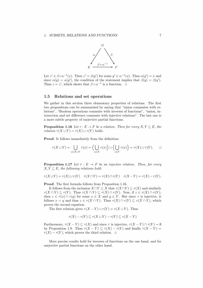
Let z′ ∈ β ◦α−1(x). Then z′ = β(y′) for some y′ ∈ α−1(x). Thus α(y′) = x andsince α(y) = α(y′), the condition of the statement implies that β(y) = β(y′).Thus z = z′, which shows that β ◦ α−1 is a function.
1.5 Relations and set operations
We gather in this section three elementary properties of relations. The firsttwo propositions can be summarised by saying that “union commutes with re-lations”, “Boolean operations commute with inverses of functions”, “union, in-tersection and set difference commute with injective relations”. The last one isa more subtle property of surjective partial functions.
Proposition 1.16 Let τ : E → F be a relation. Then for every X,Y ⊆ E, therelation τ(X ∪ Y ) = τ(X) ∪ τ(Y ) holds.
Proof. It follows immediately from the definition:
τ(X ∪ Y ) =⋃
z∈X∪Y
τ(x) =( ⋃
z∈X
τ(x))∪(⋃
z∈Y
τ(x))= τ(X) ∪ τ(Y ).
Proposition 1.17 Let τ : E → F be an injective relation. Then, for everyX,Y ⊆ E, the following relations hold:
τ(X ∪Y ) = τ(X)∪ τ(Y ) τ(X ∩Y ) = τ(X)∩ τ(Y ) τ(X−Y ) = τ(X)− τ(Y ).
Proof. The first formula follows from Proposition 1.16.It follows from the inclusion X∩Y ⊆ X that τ(X∩Y ) ⊆ τ(X) and similarly
τ(X ∩ Y ) ⊆ τ(Y ). Thus τ(X ∩ Y ) ⊆ τ(X) ∩ τ(Y ). Now, if z ∈ τ(X) ∩ τ(Y ),then z ∈ τ(x) ∩ τ(y) for some x ∈ X and y ∈ Y . But since τ is injective, itfollows x = y and thus z ∈ τ(X ∩ Y ). Thus τ(X) ∩ τ(Y ) ⊆ τ(X ∩ Y ), whichproves the second equation.
The first relation gives τ(X − Y ) ∪ τ(Y ) = τ(X ∪ Y ). Thus
τ(X)− τ(Y ) ⊆ τ(X ∪ Y )− τ(Y ) ⊆ τ(X − Y )
Furthermore, τ(X − Y ) ⊆ τ(X) and since τ is injective, τ(X − Y ) ∩ τ(Y ) = ∅by Proposition 1.9. Thus τ(X − Y ) ⊆ τ(X) − τ(Y ) and finally τ(X − Y ) =τ(X)− τ(Y ), which proves the third relation.
More precise results hold for inverses of functions on the one hand, and forsurjective partial functions on the other hand.
8 CHAPTER I. ALGEBRAIC PRELIMINARIES
Proposition 1.18 Let ϕ : E → F be a function. Then, for every X,Y ⊆ F ,the following relations hold:
ϕ−1(X ∪ Y ) = ϕ−1(X) ∪ ϕ−1(Y )
ϕ−1(X ∩ Y ) = ϕ−1(X) ∩ ϕ−1(Y )
ϕ−1(Xc) = (ϕ−1(X))c.
Proof. By Proposition 1.8, the relation ϕ−1 is injective and thus Proposition1.17 gives the first two formulas. The third one relies on the fact that ϕ−1(F ) =E. Indeed, the third property of Proposition 1.17 gives ϕ−1(Xc) = ϕ−1(F −X) = ϕ−1(F )− ϕ−1(X) = E − ϕ−1(X) = (ϕ−1(X))c.
Proposition 1.19 Let ϕ : E → F be a partial function. Then for every X ⊆ Eand Y ⊆ F , the following relation hold:
ϕ(X) ∩ Y = ϕ(X ∩ ϕ−1(Y )
)
Proof. Clearly, ϕ(X ∩ ϕ−1(Y )
)⊆ ϕ(X) and ϕ
(X ∩ ϕ−1(Y )
)⊆ ϕ(ϕ−1(Y )) ⊆
Y . Thus ϕ(X) ∩ Y ⊆ ϕ(X) ∩ Y . Moreover, if y ∈ ϕ(X) ∩ Y , then y = ϕ(x)for some x ∈ X and since y ∈ Y , x ∈ ϕ−1(Y ). It follows that ϕ(X) ∩ Y ⊆ϕ(X ∩ ϕ−1(Y )
), which concludes the proof.
2 Ordered sets
If R is a relation on E, two elements x and y of E are said to be related by Rif (x, y) ∈ R, which is also denoted by x R y.
A relation R is reflexive if, for each x ∈ E, x R x, symmetric if, for eachx, y ∈ E, x R y implies y R x, antisymmetric if, for each x, y ∈ E, x R y andy R x imply x = y and transitive if, for each x, y, z ∈ E, x R y and y R zimplies x R z.
A relation is a preorder if it is reflexive and transitive, an order (or partialorder) if it is reflexive, transitive and antisymmetric and an equivalence relation(or an equivalence) if it is reflexive, transitive and symmetric. If R is a preorder,the relation ∼ defined by x ∼ y if and only if x R y and y R x is an equivalencerelation, called the equivalence relation associated with R.
Relations are ordered by inclusion. More precisely, if R1 and R2 are tworelations on a set S, R1 refines R2 (or R1 is thinner than R2, or R2 is coarserthan R1) if and only if, for each s, t ∈ S, s R1 t implies s R2 t. Equality isthus the thinnest equivalence relation and the universal relation, in which allelements are related, is the coarsest. The following property is obvious.
Proposition 2.20 Any intersection of preorders is a preorder. Any intersec-tion of equivalence relations is an equivalence relation.
It follows that, given a set R of relations on a set E, there is a smallestpreorder [equivalence relation] containing all the relations of E. This relation iscalled the preorder [equivalence relation] generated by R.
Proposition 2.21 Let R1 and R2 be two preorders [equivalence relations ] ona set E. If they commute, the preorder [equivalence relation] generated by R1
and R2 is equal to R1 ◦ R2.
3. EXERCISES 9
Proof. Suppose that R1 and R2 commute and let R = R1 ◦ R2. Then R isclearly reflexive but it is also transitive. Indeed, if x1 R x2 and x2 R x3, thereexist y1, y2 ∈ E such that x1 R1 y1, y1 R2 x2, x2 R1 y2 and y2 R2 x3. SinceR = R2 ◦ R1, one gets y1 R y2 and since R1 and R2 commute, there exists ysuch that y1 R1 y and y R2 y2. It follows that x1 R1 y and y R2 x3 and thusx1 R x3.
An upper set of an ordered set (E,6) is a subset F of E such that, if x 6 yand x ∈ F , then y ∈ F . The upper set generated by an element x is the set ↑xof all y ∈ E such that x 6 y. The intersection [union] of any family of uppersets is also an upper set.
A chain is a totally ordered subset of a partially ordered set.
3 Exercises
1. Let ϕ1 : E1 → E2, ϕ2 : E2 → E3 and ϕ3 : E3 → E1 be three functions.Show that if, among the mappings ϕ3 ◦ ϕ2 ◦ ϕ1, ϕ2 ◦ ϕ1 ◦ ϕ3, and ϕ1 ◦ ϕ3 ◦ ϕ2,two are surjective and the third is injective, or two are injective and the thirdis surjective, then the three functions ϕ1, ϕ2 and ϕ3 are bijective.
2. This exercise is due to J. Almeida [3, Lemma 8.2.5].Let X and Y be two totally ordered finite sets and let P be a partially orderedset. Let ϕ : X → Y , γ : Y → X, π : X → P and θ : Y → P be functions suchthat:
(1) for any x ∈ X, π(x) 6 θ(ϕ(x)),
(2) for any y ∈ Y , θ(y) 6 π(γ(y)),
(3) if x1, x2 ∈ X, ϕ(x1) = ϕ(x2) and π(x1) = θ(ϕ(x1)), then x1 = x2,
(4) if y1, y2 ∈ Y , γ(y1) = γ(y2) and θ(y1) = π(γ(y1)), then y1 = y2.
Then ϕ and γ are mutually inverse functions, π = θ ◦ ϕ and θ = π ◦ γ.

10 CHAPTER I. ALGEBRAIC PRELIMINARIES
Chapter II
Semigroups and beyond
The purpose of this chapter is to introduce the basic algebraic definitions thatwill be used in this book: semigroups, monoids, groups and semirings, mor-phisms, substructures and quotients for these structures, transformation semi-groups and free semigroups. We also devote a short section to idempotents, acentral notion in finite semigroup theory.
1 Semigroups, monoids and groups
1.1 Semigroups, monoids
Let S be a set. A binary operation on S is a mapping from S × S into S. Theimage of (x, y) under this mapping is often denoted by xy and is called theproduct of x and y. In this case, it is convenient to call the binary operationmultiplication. Sometimes, the additive notation x+y is adopted, the operationis called addition and x+ y denotes the sum of x and y.
An operation on S is associative if, for every x, y, z in S, (xy)z = x(yz). Itis commutative, if, for every x, y in S, xy = yx.
An element 1 of S is called an identity element or simply identity or unitfor the operation if, for all x ∈ S, x1 = x = 1x. It is easy to see there canbe at most one identity, which is then called the identity. Indeed if 1 and 1′
are two identities, one has simultaneously 11′ = 1′, since 1 is an identity, and11′ = 1, since 1′ is an identity, whence 1 = 1′. In additive notation, the identityis denoted by 0 to get the intuitive formula 0 + x = x = x+ 0.
A semigroup is a pair consisting of a set S and an associative binary operationon S. A semigroup is a pair, but we shall usually say “S is a semigroup” andassume the binary operation is known. A monoid is a triple consisting of a setM , an associative binary operation onM and an identity for this operation. Thenumber of elements of a semigroup is often called its order1. Thus a semigroupof order 4 is a semigroup with 4 elements.
The dual semigroup of a semigroup S, denoted by S, is the semigroup definedon the set S by the operation ∗ given by s ∗ t = ts.
A semigroup [monoid, group] is said to be commutative if its operation iscommutative.
1This well-established terminology has of course nothing to do with the order relations.
11
12 CHAPTER II. SEMIGROUPS AND BEYOND
If S is a semigroup, let S1 denote the monoid equal to S if S is a monoid,and to S ∪ {1} if S is not a monoid. In the latter case, the operation of S iscompleted by the rules
1s = s1 = s
for each s ∈ S1.
1.2 Special elements
Being idempotent, zero and cancellable are the three important properties ofan element of a semigroup defined in this section. We also define the notionof semigroup inverse of an element. Regular elements, which form anotherimportant category of elements, will be introduced in Section V.2.2.
Idempotents
Let S be a semigroup. An element e of S is an idempotent if e = e2. The set ofidempotents of S is denoted by E(S). We shall see later that idempotents playa fundamental role in the study of finite semigroups.
An element e of S is a right identity [left identity] of S if, for all s ∈ S, se = s[es = s]. Observe that e is an identity if and only if it is simultaneously a rightand a left identity. Furthermore, a right [left] identity is necessarily idempotent.The following elementary result illustrates these notions.
Proposition 1.1 (Simplification lemma) Let S be a semigroup. Let s ∈ Sand e, f be idempotents of S1. If s = esf , then es = s = sf .
Proof. If s = esf , then es = eesf = esf = s and sf = esff = esf = s.
Zeros
An element e is said to be a zero [right zero, left zero] if, for all s ∈ S, es = e = se[se = e, es = e].
Proposition 1.2 A semigroup has at most one zero element.
Proof. Assume that e and e′ are zero elements of a semigroup S. Then bydefinition, e = ee′ = e′ and thus e = e′.
If S is a semigroup, let S0 denote the semigroup obtained from S by additionof a zero: the support2 of S0 is the disjoint union of S and the singleton3 0 andthe multiplication (here denoted by ∗) is defined by
s ∗ t =
{st if s, t ∈ S
0 if s = 0 or t = 0.
A semigroup is called null if it has a zero and if the product of two elements isalways zero.
2That is, the set on which the semigroup is defined.3A singleton {s} will also be denoted by s.

1. SEMIGROUPS, MONOIDS AND GROUPS 13
Cancellative elements
An element s of a semigroup S is said to be right cancellative [left cancellative]if, for every x, y ∈ S, the condition xs = ys [sx = sy] implies x = y. It iscancellative if it is simultaneously right and left cancellative.
A semigroup S is right cancellative [left cancellative, cancellative] if all itselements are right cancellative [left cancellative, cancellative].
Inverses
We have to face a slight terminology problem with the notion of an inverse.Indeed, semigroup theorists have coined a notion of inverse that differs from thestandard notion used in group theory and elsewhere in mathematics. Usually,the context should permit to clarify which definition is understood. But to avoidany ambiguity, we shall use the terms group inverse and semigroup inverse whenwe need to distinguish the two notions.
Let M be a monoid. A right group inverse [left group inverse] of an elementx of M is an element x′ such that xx′ = 1 [x′x = 1]. A group inverse of x is anelement x′ which is simultaneously a right and left group inverse of x, so thatxx′ = x′x = 1.
We now come to the notion introduced by semigroup theorists. Given anelement x of a semigroup S, an element x′ is a semigroup inverse or simplyinverse of x if xx′x = x and x′xx′ = x′.
It is clear that any group inverse is a semigroup inverse but the converse isnot true. A thorough study of semigroup inverses will be given in Section V.2,but let us warn the reader immediately of some counterintuitive facts aboutinverses. An element of an infinite monoid may have several right group inversesand several left group inverses. The situation is radically different for a finitemonoid: each element has at most one left [right] group inverse and if theseelements exist, they are equal. However, an element of a semigroup (finite orinfinite) may have several semigroup inverses, or no semigroup inverse at all.
1.3 Groups
A monoid is a group if each of its elements has a group inverse. A slightly weakercondition can be given.
Proposition 1.3 A monoid is a group if and only if each of its elements has aright group inverse and a left group inverse.
Proof. In a group, every element has a right group inverse and a left groupinverse. Conversely, let G be a monoid in which every element has a rightgroup inverse and a left group inverse. Let g ∈ G, let g′ [g′′] be a right [left]inverse of g. Thus, by definition, gg′ = 1 and g′′g = 1. It follows that g′′ =g′′(gg′) = (g′′g)g′ = g′. Thus g′ = g′′ is an inverse of g. Thus G is a group.
For finite monoids, this result can be further strengthened as follows:
Proposition 1.4 A finite monoid G is a group if and only if every element ofG has a left group inverse.
14 CHAPTER II. SEMIGROUPS AND BEYOND
Of course, the dual statement for right group inverses hold.
Proof. Let G be a finite monoid in which every element has a left group inverse.Given an element g ∈ G, consider the map ϕ : G → G defined by ϕ(x) = gx.We claim that ϕ is injective. Suppose that gx = gy for some x, y ∈ G and letg′ be the left group inverse of g. Then g′gx = g′gy, that is x = y, provingthe claim. Since G is finite, Proposition I.1.7 shows that ϕ is also surjective.In particular, there exists an element g′′ ∈ G such that 1 = gg′′. Thus everyelement of G has a right group inverse and by Proposition 1.3, G is a group.
Proposition 1.5 A group is a cancellative monoid. In a group, every elementhas a unique group inverse.
Proof. Let G be a group. Let g, x, y ∈ G and let g′ be a group inverse of g.If gx = gy, then g′gx = g′gy, that is x = y. Similarly, xg = yg implies x = yand thus G is cancellative. In particular, if g′ and g′′ are two group inversesof g, gg′ = gg′′ and thus g′ = g′′. Thus every element has a unique inverse.
In a group, the unique group inverse of an element x is denoted by x−1 and iscalled the inverse of x. Thus xx−1 = x−1x = 1. It follows that the equationgx = h [xg = h] has a unique solution: x = g−1h [x = hg−1].
1.4 Ordered semigroups and monoids
An ordered semigroup is a semigroup S equipped with an order relation 6 onS which is compatible with the product: for every x, y ∈ S, for every u, v ∈ S1
x 6 y implies uxv 6 uyv.
The notation (S,6) will sometimes be used to emphasize the role of theorder relation, but most of the time the order will be implicit and the notationS will be used for semigroups as well as for ordered semigroups. If (S,6) is anordered semigroup, then (S,>) is also an ordered semigroup. Ordered monoidsare defined analogously.
1.5 Semirings
A semiring is a quintuple consisting of a set k, two binary operations on k,written additively and multiplicatively, and two elements 0 and 1, satisfying thefollowing conditions:
(1) k is a commutative monoid for the addition with identity 0,
(2) k is a monoid for the multiplication with identity 1,
(3) Multiplication is distributive over addition: for all s, t1, t2 ∈ k, s(t1+t2) =st1 + st2 and (t1 + t2)s = t1s+ t2s,
(4) for all s ∈ k, 0s = s0 = 0.
A ring is a semiring in which the monoid (k,+, 0) is a group. A semiring iscommutative if its multiplication is commutative.
2. EXAMPLES 15
2 Examples
We give successively some examples of semigroups, monoids, groups, orderedmonoids and semirings.
2.1 Examples of semigroups
(1) The set N+ of positive integers is a commutative semigroup for the usualaddition of integers. It is also a commutative semigroup for the usualmultiplication of integers.
(2) Let I and J be two nonempty sets. Define an operation on I × J bysetting, for every (i, j), (i′, j′) ∈ I × J ,
(i, j)(i′, j′) = (i, j′)
This defines a semigroup, usually denoted by B(I, J).
(3) Let n be a positive integer. Let Bn be the set of all matrices of size n× nwith zero-one entries and at most one nonzero entry. Equipped with theusual multiplication of matrices, Bn is a semigroup. For instance,
B2 =
{(1 00 0
),
(0 10 0
),
(0 01 0
),
(0 00 1
),
(0 00 0
)}
This semigroup is nicknamed the universal counterexample because it pro-vides many counterexamples in semigroup theory. Setting a = ( 0 1
0 0 )and b = ( 0 0
1 0 ), one gets ab = ( 1 00 0 ), ba = ( 0 0
0 1 ) and 0 = ( 0 00 0 ). Thus
B2 = {a, b, ab, ba, 0}. Furthermore, the relations aa = bb = 0, aba = a andbab = b suffice to recover completely the multiplication in B2.
(4) Let S be a set. Define an operation on S by setting st = s for everys, t ∈ S. Then every element of S is a left zero, and S forms a left zerosemigroup.
(5) Let S be the semigroup of matrices of the form(a 0b 1
)
where a and b are positive rational numbers, under matrix multiplication.We claim that S is a cancellative semigroup without identity. Indeed,since (
a 0b 1
)(x 0y 1
)=
(ax 0
bx+ y 1
)
it follows that if(a 0b 1
)(x1 0y1 1
)=
(a 0b 1
)(x2 0y2 1
)
then ax1 = ax2 and bx1+y1 = bx2+y2, whence x1 = x2 and y1 = y2, whichproves that S is left cancellative. The proof that S is right cancellative isdual.
(6) If S is a semigroup, the set P(S) of subsets of S is also a semigroup, forthe multiplication defined, for every X,Y ∈ P(S), by
XY = {xy | x ∈ X, y ∈ Y }

16 CHAPTER II. SEMIGROUPS AND BEYOND
2.2 Examples of monoids
(1) The trivial monoid, denoted by 1, consists of a single element, the identity.
(2) The set N of nonnegative integers is a commutative monoid for the ad-dition, whose identity is 0. It is also a commutative monoid for the maxoperation, whose identity is also 0 and for the multiplication, whose iden-tity is 1.
(3) The monoid U1 = {1, 0} defined by its multiplication table 1 ∗ 1 = 1 and0 ∗ 1 = 0 ∗ 0 = 1 ∗ 0 = 0.
(4) More generally, for each nonnegative integer n, the monoid Un is defined onthe set {1, a1, . . . , an} by the operation aiaj = aj for each i, j ∈ {1, . . . , n}and 1ai = ai1 = ai for 1 6 i 6 n.
(5) The monoid Un has the same underlying set as Un, but the multiplicationis defined in the opposite way: aiaj = ai for each i, j ∈ {1, . . . , n} and1ai = ai1 = ai for 1 6 i 6 n.
(6) The monoid B12 is obtained from the semigroup B2 by adding an identity.
Thus B12 = {1, a, b, ab, ba, 0} where aba = a, bab = b and aa = bb = 0.
(7) The bicyclic monoid is the monoid M = {(i, j) | (i, j) ∈ N2} under theoperation
(i, j)(i′, j′) = (i+ i′ −min(j, i′), j + j′ −min(j, i′))
2.3 Examples of groups
(1) The set Z of integers is a commutative group for the addition, whoseidentity is 0.
(2) The set Z/nZ of integers modulo n, under addition is also a commutativegroup.
(3) The set of 2× 2 matrices with entries in Z and determinant ±1 is a groupunder the usual multiplication of matrices. This group is denoted byGL2(Z).
2.4 Examples of ordered monoids
(1) Every monoid can be equipped with the equality order, which is compati-ble with the product. It is actually often convenient to consider a monoidM as the ordered monoid (M,=).
(2) The natural order on nonnegative integers is compatible with addition andwith the max operation. Thus (N,+,6) and (N,max,6) are both orderedmonoids.
(3) We let U+1 [U−
1 ] denote the monoid U1 = {1, 0} ordered by 1 < 0 [0 < 1].
2.5 Examples of semirings
(1) Rings are the first examples of semirings that come to mind. In particular,we let Z, Q and R, respectively, denote the rings of integers, rational andreal numbers.

3. BASIC ALGEBRAIC STRUCTURES 17
(2) The simplest example of a semiring which is not a ring is the Booleansemiring B = {0, 1} whose operations are defined by the following tables
+ 0 1
0 0 1
1 1 1
× 0 1
0 0 0
1 0 1
(3) If M is a monoid, then the set P(M) of subsets of M is a semiring withunion as addition and multiplication given by
XY = {xy | x ∈ X and y ∈ Y }
The empty set is the zero and the unit is the singleton {1}.
(4) Other examples include the semiring of nonnegative integers N = (N,+,×)and its completion N = (N ∪ {∞},+,×), where addition and multiplica-tion are extended in the natural way
for all x ∈ N , x+∞ =∞+ x =∞
for all x ∈ N − {0}, x×∞ =∞× x =∞
∞× 0 = 0×∞ = 0
(5) The Min-Plus semiring is M = (N ∪ {∞},min,+). This means that inthis semiring the sum is defined as the minimum and the product as theusual addition. Note that ∞ is the zero of this semiring and 0 is its unit.
3 Basic algebraic structures
3.1 Morphisms
On a general level, a morphism between two algebraic structures is a map pre-serving the operations. Therefore a semigroup morphism is a map ϕ from asemigroup S into a semigroup T such that, for every s1, s2 ∈ S,
(1) ϕ(s1s2) = ϕ(s1)ϕ(s2).
Similarly, a monoid morphism is a map ϕ from a monoid S into a monoid Tsatisfying (1) and
(2) ϕ(1) = 1.
A morphism of ordered monoids is a map ϕ from an ordered monoid (S,6) intoa monoid (T,6) satisfying (1), (2) and, for every s1, s2 ∈ S such that s1 6 s2,
(3) ϕ(s1) 6 ϕ(s2).
Formally, a group morphism between two groupsG andG′ is a monoid morphismϕ satisfying, for every s ∈ G, ϕ(s−1) = ϕ(s)−1. In fact, this condition can berelaxed.
Proposition 3.6 Let G and G′ be groups. Then any semigroup morphism fromG to G′ is a group morphism.
Proof. Let ϕ : G → G′ be a semigroup morphism. Then by (1), ϕ(1) =ϕ(1)ϕ(1) and thus ϕ(1) = 1 since 1 is the unique idempotent of G′. Thus ϕis a monoid morphism. Furthermore, ϕ(s−1)ϕ(s) = ϕ(s−1s) = ϕ(1) = 1 andsimilarly ϕ(s)ϕ(s−1) = ϕ(ss−1) = ϕ(1) = 1.

18 CHAPTER II. SEMIGROUPS AND BEYOND
A semiring morphism between two semirings k and k′ is a map ϕ : k → k′
which is a monoid morphism for the additive structure and for the multiplicativestructure.
The semigroups [monoids, groups, ordered monoids, semirings], togetherwith the morphisms defined above, form a category. We shall encounter inChapter XIII another interesting category whose objects are semigroups andwhose morphisms are called relational morphisms.
A morphism ϕ : S → T is an isomorphism if there exists a morphism ψ :T → S such that ϕ ◦ ψ = IdT and ψ ◦ ϕ = IdS .
Proposition 3.7 In the category of semigroups [monoids, groups, semirings ],a morphism is an isomorphism if and only if it is bijective.
Proof. If ϕ : S → T an isomorphism, then ϕ is bijective since there exists amorphism ψ : T → S such that ϕ ◦ ψ = IdT and ψ ◦ ϕ = IdS .
Suppose now that ϕ : S → T is a bijective morphism. Then ϕ−1 is amorphism from T into S, since, for each x, y ∈ T ,
ϕ(ϕ−1(x)ϕ−1(y)) = ϕ(ϕ−1(x))ϕ(ϕ−1(y)) = xy
Thus ϕ is an isomorphism.
Proposition 3.7 does not hold for morphisms of ordered monoids. In partic-ular, if (M,6) is an ordered monoid, the identity induces a bijective morphismfrom (M,=) onto (M,6) which is not in general an isomorphism. In fact, amorphism of ordered monoids ϕ :M → N is an isomorphism if and only if ϕ isa bijective monoid morphism and, for every x, y ∈ M , x 6 y is equivalent withϕ(x) 6 ϕ(y).
Two semigroups [monoids, ordered monoids] are isomorphic if there existsan isomorphism from one to the other. As a general rule, we shall identify twoisomorphic semigroups.
3.2 Subsemigroups
A subsemigroup of a semigroup S is a subset T of S such that s1 ∈ T and s2 ∈ Timply s1s2 ∈ T . A submonoid of a monoid is a subsemigroup containing theidentity. A subgroup of a group is a submonoid containing the inverse of eachof its elements.
A subsemigroup G of a semigroup S is said to be a group in S if there isan idempotent e ∈ G such that G, under the operation of S, is a group withidentity e.
Proposition 3.8 Let ϕ : S → T be a semigroup morphism. If S′ is a subsemi-group of S, then ϕ(S′) is a subsemigroup of T . If T ′ is a subsemigroup of T ,then ϕ−1(T ′) is a subsemigroup of S.
Proof. Let t1, t2 ∈ ϕ(S′). Then t1 = ϕ(s1) and t2 = ϕ(s2) for some s1, s2 ∈ S
′.Since S′ is a subsemigroup of S, s1s2 ∈ S
′ and thus ϕ(s1s2) ∈ ϕ(S′). Now since
ϕ is a morphism, ϕ(s1s2) = ϕ(s1)ϕ(s2) = t1t2. Thus t1t2 ∈ ϕ(S′) and ϕ(S′) isa subsemigroup of T .

3. BASIC ALGEBRAIC STRUCTURES 19
Let s1, s2 ∈ ϕ−1(T ′). Then ϕ(s1), ϕ(s2) ∈ T ′ and since T ′ is a subsemigroupof T , ϕ(s1)ϕ(s2) ∈ T
′. Since ϕ is a morphism, ϕ(s1)ϕ(s2) = ϕ(s1s2) and thuss1s2 ∈ ϕ
−1(T ′). Therefore ϕ−1(T ′) is a subsemigroup of S.
Proposition 3.8 can be summarised as follows: substructures are preservedby morphisms and by inverses of morphisms. A similar statement holds formonoid morphisms and for group morphisms.
3.3 Quotients and divisions
Let S and T be two semigroups [monoids, groups, ordered monoids]. Then T isa quotient of S if there exists a surjective morphism from S onto T .
Note that any ordered monoid (M,6) is a quotient of the ordered monoid(M,=), since the identity on M is a morphism of ordered monoid from (M,=)onto (M,6).
Finally, a semigroup T divides a semigroup S (notation T 4 S) if T is aquotient of a subsemigroup of S.
Proposition 3.9 The division relation is transitive.
Proof. Suppose that S1 4 S2 4 S3. Then there exists a subsemigroup T1of S2, a subsemigroup T2 of S3 and surjective morphisms π1 : T1 → S1 andπ2 : T2 → S2. Put T = π−1
2 (T1). Then T is a subsemigroup of S3 and S1
is a quotient of T since π1(π2(T )) = π1(T1) = S1. Thus S1 divides S3.
The next proposition shows that division is a partial order on finite semigroups,up to isomorphism.
Proposition 3.10 Two finite semigroups that divide each other are isomorphic.
Proof. We keep the notation of the proof of Proposition 3.9, with S3 = S1.Since T1 is a subsemigroup of S2 and T2 is a subsemigroup of S1, one has |T1| 6|S2| and |T2| 6 |S1|. Furthermore, since π1 and π2 are surjective, |S1| 6 |T1|and |S2| 6 |T2|. It follows that |S1| = |T1| = |S2| = |T2|, whence T1 = S2
and T2 = S1. Furthermore, π1 and π2 are bijections and thus S1 and S2 areisomorphic.
The term division stems from a property of finite groups, usually known asLagrange’s theorem. The proof is omitted but is not very difficult and can befound in any textbook on finite groups.
Proposition 3.11 (Lagrange) Let G and H be finite groups. If G divides H,then |G| divides |H|.
The use of the term division in semigroup theory is much more questionablesince Lagrange’s theorem does not extend to finite semigroups. However, thisterminology is universally accepted and we shall stick to it.
Let us mention a few useful consequences of Lagrange’s theorem.
Proposition 3.12 Let G be a finite group. Then, for each g ∈ G, g|G| = 1.

20 CHAPTER II. SEMIGROUPS AND BEYOND
Proof. Consider the set H of all powers of g. Since G is finite, two powers, saygp and gq with q > p, are equal. Since G is a group, it follows that gq−p = 1. Letr be the smallest positive integer such that gr = 1. Then H = {1, g, . . . , gr−1}is a cyclic group and by Lagrange’s theorem, |G| = rs for some positive integers. It follows that g|G| = (gr)s = 1s = 1.
Proposition 3.13 A nonempty subsemigroup of a finite group is a subgroup.
Proof. Let G be a finite group and let S be a nonempty subsemigroup of G.Let s ∈ S. By Proposition 3.12, s|G| = 1. Thus 1 ∈ S. Consider now the mapϕ : S → S defined by ϕ(x) = xs. It is injective, for G is right cancellative, andhence bijective by Proposition I.1.7. Consequently, there exists an element s′
such that s′s = 1. Thus every element has a left inverse and by Proposition 1.4,S is a group.
3.4 Products
Given a family (Si)i∈I of semigroups [monoids, groups], the product Πi∈ISi isthe semigroup [monoid, group] defined on the cartesian product of the sets Si
by the operation(si)i∈I(s
′i)i∈I = (sis
′i)i∈I
Note that the semigroup 1 is the identity for the product of semigroups [monoids,groups]. Following a usual convention, which can also be justified in the frame-work of category theory, we put
∏i∈∅ Si = 1.
Given a family (Mi)i∈I of ordered monoids, the product∏
i∈I Mi is naturallyequipped with the order
(si)i∈I 6 (s′i)i∈I if and only if, for all i ∈ I, si 6 s′i.
The resulting ordered monoid is the product of the ordered monoids (Mi)i∈I .The next proposition, whose proof is obvious, shows that product preserves
substructures, quotients and division. We state it for semigroups, but it can bereadily extended to monoids and to ordered semigroups or monoids.
Proposition 3.14 Let (Si)i∈I and (Ti)i∈I be two families of semigroups suchthat, for each i ∈ I, Si is a subsemigroup [quotient, divisor ] of Ti. Then
∏i∈I Si
is a subsemigroup of [quotient, divisor ] of∏
i∈I Ti.
3.5 Ideals
Let S be a semigroup. A right ideal of S is a subset R of S such that RS ⊆ R.Thus R is a right ideal if, for each r ∈ R and s ∈ S, rs ∈ R. Symmetrically, aleft ideal is a subset L of S such that SL ⊆ L. An ideal is a subset of S whichis simultaneously a right and a left ideal.
Observe that a subset I of S is an ideal if and only if, for every s ∈ I andx, y ∈ S1, xsy ∈ I. Here, the use of S1 instead of S allows us to include thecases x = 1 and y = 1, which are necessary to recover the conditions SI ⊆ Sand IS ⊆ I. Slight variations on the definition are therefore possible:
(1) R is a right ideal if and only if RS1 ⊆ R or, equivalently, RS1 = R,
(2) L is a left ideal if and only if S1L ⊆ L or, equivalently, S1L = L,
3. BASIC ALGEBRAIC STRUCTURES 21
(3) I is an ideal if and only if S1IS1 ⊆ I or, equivalently, S1IS1 = I.
Note that any intersection of ideals [right ideals, left ideals] of S is again anideal [right ideal, left ideal].
Let R be a subset of a semigroup S. The ideal [right ideal, left ideal] gen-erated by R is the set S1RS1 [RS1, S1R]. It is the smallest ideal [right ideal,left ideal] containing R. An ideal [right ideal, left ideal] is called principal ifit is generated by a single element. Note that the ideal [right ideal, left ideal]generated by an idempotent e is equal to SeS [eS, Se]. Indeed, the equalityS1eS1 = SeS follows from the fact that e = eee.
Ideals are stable under surjective morphisms and inverses of morphisms.
Proposition 3.15 Let ϕ : S → T be a semigroup morphism. If J is an ideal ofT , then ϕ−1(J) is a ideal of S. Furthermore, if ϕ is surjective and I is an idealof S, then ϕ(I) is an ideal of T . Similar results apply to right and left ideals.
Proof. If J is an ideal of T , then
S1ϕ−1(J)S1 ⊆ ϕ−1(T 1)ϕ−1(J)ϕ−1(T 1) ⊆ ϕ−1(T 1JT 1) ⊆ ϕ−1(J)
Thus ϕ−1(J) is an ideal of S.Suppose that ϕ is surjective. If I is an ideal of S, then
T 1ϕ(I)T 1 = ϕ(S1)ϕ(I)ϕ(S1) = ϕ(S1IS1) = ϕ(I)
Thus ϕ(I) is an ideal of T .
Let, for 1 6 k 6 n, Ik be an ideal of a semigroup S. The set
I1I2 · · · In = {s1s2 · · · sn | s1 ∈ I1, s2 ∈ I2, . . . , sn ∈ In}
is the product of the ideals I1, . . . , In.
Proposition 3.16 The product of the ideals I1, . . . , In is an ideal contained intheir intersection.
Proof. Since I1 and In are ideals, S1I1 = I1 and InS1 = In. Therefore
S1(I1I2 · · · In)S1 = (S1I1)I2 · · · (InS
1) = I1I2 · · · In
and thus I1I2 · · · In is an ideal. Furthermore, for 1 6 k 6 n, I1I2 · · · In ⊆S1IkS
1 = Ik. Thus I1I2 · · · In is contained in⋂
16k6n Ik.
A nonempty ideal I of a semigroup S is called minimal if, for every nonemptyideal J of S, J ⊆ I implies J = I.
Proposition 3.17 A semigroup has at most one minimal ideal.
Proof. Let I1 and I2 be two minimal ideals of a semigroup S. Then by Propo-sition 3.16, I1I2 is a nonempty ideal of S contained in I1 ∩ I2. Now since I1 andI2 are minimal ideals, I1I2 = I1 = I2.
The existence of a minimal ideal is assured in two important cases, namelyif S is finite or if S possesses a zero. In the latter case, 0 is the minimal ideal. Anonempty ideal I 6= 0 such that, for every nonempty ideal J of S, J ⊆ I impliesJ = 0 or J = I is called a 0-minimal ideal. It should be noted that a semigroupmay have several 0-minimal ideals as shown in the next example.
22 CHAPTER II. SEMIGROUPS AND BEYOND
Example 3.1 Let S = {s, t, 0} be the semigroup defined by xy = 0 for everyx, y ∈ S. Then 0 is the minimal ideal of S and {s, 0} and {t, 0} are two 0-minimalideals.
3.6 Simple and 0-simple semigroups
A semigroup S is called simple if its only ideals are ∅ and S. It is called 0-simple if it has a zero, denoted by 0, if S2 6= {0} and if ∅, 0 and S are its onlyideals. The notions of right simple, right 0-simple, left simple and left 0-simplesemigroups are defined analogously.
Lemma 3.18 Let S be a 0-simple semigroup. Then S2 = S.
Proof. Since S2 is a nonempty, nonzero ideal, one has S2 = S.
Proposition 3.19
(1) A semigroup S is simple if and only if SsS = S for every s ∈ S.
(2) A semigroup S is 0-simple if and only if S 6= ∅ and SsS = S for everys ∈ S − 0.
Proof. We shall prove only (2), but the proof of (1) is similar.Let S be a 0-simple semigroup. Then S2 = S by Lemma 3.18 and hence
S3 = S.Let I be set of the elements s of S such that SsS = 0. This set is an ideal of
S containing 0, but not equal to S since⋃
s∈S SsS = S3 = S. Therefore I = 0.In particular, if s 6= 0, then SsS 6= 0, and since SsS is an ideal of S, it followsthat SsS = S.
Conversely, if S 6= ∅ and SsS = S for every s ∈ S−0, we have S = SsS ⊆ S2
and therefore S2 6= 0. Moreover, if J is a nonzero ideal of S, it contains anelement s 6= 0. We then have S = SsS ⊆ SJS = J , whence S = J . ThereforeS is 0-simple.
The structure of finite simple semigroups will be detailed in Section V.3.
3.7 Semigroup congruences
A semigroup congruence is a stable equivalence relation. Thus an equivalencerelation ∼ on a semigroup S is a congruence if, for each s, t ∈ S and u, v ∈ S1,we have
s ∼ t implies usv ∼ utv.
The set S/∼ of equivalence classes of the elements of S is naturally equippedwith the structure of a semigroup, and the function which maps every elementonto its equivalence class is a semigroup morphism from S onto S/∼. Fourparticular cases of congruences are extensively used.
(a) Rees congruence
Let I be an ideal of a semigroup S and let ≡I be the equivalence relationidentifying all the elements of I and separating the other elements. Formally,s ≡I t if and only if s = t or s, t ∈ I. Then ≡I is a congruence called theRees congruence of I. The quotient of S by ≡I is usually denoted by S/I. The

3. BASIC ALGEBRAIC STRUCTURES 23
support of this semigroup is the set (S − I) ∪ 0 and the multiplication (heredenoted by ∗) is defined by
s ∗ t =
{st if s, t ∈ S − I
0 if s = 0 or t = 0.
(b) Syntactic congruence
Let P be a subset of a semigroup S. The syntactic congruence of P is thecongruence ∼P over S defined by s ∼P t if and only if, for every x, y ∈ S1,
xsy ∈ P ⇐⇒ xty ∈ P
The quotient semigroup S/∼P is called the syntactic semigroup of P in S. Thesyntactic semigroup is particularly important in the theory of formal languages.
(c) Congruence generated by a relation
Let R be a relation on S, that is, a subset of S × S. The set of all congruencescontaining R is nonempty since it contains the universal relation on S. Fur-thermore, it is closed under intersection. It follows that the intersection of allcongruences containing R is a congruence, called the congruence generated byR. Let us give a more constructive definition.
Proposition 3.20 The congruence generated by a symmetric relation R on asemigroup S is the reflexive-transitive closure of the relation
{(xry, xsy) | (r, s) ∈ R and x, y ∈ S1}
Proof. If a congruence contains R, it certainly contains the relation
R = {(xry, xsy) | (r, s) ∈ R and x, y ∈ S1}
and hence its reflexive-transitive closure R∗. Therefore, it suffices to show thatR∗ is a congruence. Let (u, v) ∈ R∗. By definition, there exists a finite sequenceu = u0, u1, . . . , un = v such that
(u0, u1) ∈ R, (u1, u2) ∈ R, · · · , (un−1, un) ∈ R
Therefore, one has, for some xi, yi, ri, si ∈ S such that (ri, si) ∈ R,
(u0, u1) = (x0r0y0, x0s0y0), (u1, u2) = (x1r1y1, x1s1y1), · · · ,
(un−1, un) = (xn−1rn−1yn−1, xn−1sn−1yn−1)
Let now x, y ∈ S1. Then the relations
(xuiy, xui+1y) = (xxiriyiy, xxisiyiy) ∈ R (0 6 i 6 n− 1)
show that (xuy, xvy) ∈ R∗. Thus R∗ is a congruence.
(d) Nuclear congruence
For each semigroup morphism ϕ : S → T , the equivalence ∼ϕ defined on S by
x ∼ϕ y if and only if ϕ(x) = ϕ(y)
is a congruence. This congruence, called the nuclear congruence of ϕ, has thefollowing standard property.

24 CHAPTER II. SEMIGROUPS AND BEYOND
Proposition 3.21 (First isomorphism theorem) Let ϕ : S → T be a mor-phism of semigroups and let π : S → S/∼ϕ be the quotient morphism. Thenthere exists a unique semigroup morphism ϕ : S/∼ϕ → T such that ϕ = ϕ ◦ π.Moreover, ϕ is an isomorphism from S/∼ϕ onto ϕ(S).
Proof. The situation is summed up in the following diagram:
S/∼ϕ T
S
π
ϕ
ϕ
Uniqueness is clear: if s is the ∼ϕ-class of some element x, then necessarily
ϕ(s) = ϕ(x) (3.1)
Furthermore, if x and y are arbitrary elements of s, then ϕ(x) = ϕ(y). Therefore,there is a well-defined function ϕ defined by Formula (3.1). Moreover, if π(x1) =s1 and π(x2) = s2, then π(x1x2) = s1s2, whence
ϕ(s1)ϕ(s2) = ϕ(x1)ϕ(x2) = ϕ(x1x2) = ϕ(s1s2)
Therefore ϕ is a morphism. We claim that ϕ is injective. Indeed, suppose thatϕ(s1) = ϕ(s2), and let x1 ∈ π
−1(s1) and x2 ∈ π−1(s2). Then ϕ(x1) = ϕ(x2)
and thus x1 ∼ϕ x2. It follows that π(x1) = π(x2), that is, s1 = s2. Thus ϕinduces an isomorphism from S/∼ϕ onto ϕ(S).
When two congruences are comparable, the quotient structures associatedwith them can also be compared.
Proposition 3.22 (Second isomorphism theorem) Let ∼1 and ∼2 be twocongruences on a semigroup S and π1 [π2] the canonical morphism from S ontoS/∼1 [S/∼2]. If ∼2 is coarser than ∼1, there exists a unique surjective mor-phism π : S/∼1 → S/∼2 such that π ◦ π1 = π2.
Proof. Since π ◦ π1 = π2, Corollary I.1.13 shows that π is necessarily equal tothe relation π2 ◦ π
−11 . Furthermore, Proposition I.1.15 shows that this relation
is actually a function.Since π1 and π2 are morphisms,
π(π1(s)π1(t)) = π(π1(st)) = π2(st) = π2(s)π2(t) = π(π1(s))π(π1(t))
and thus π is a morphism.
Proposition 3.23 Let S be a semigroup, (∼i)i∈I be a family of congruenceson S and ∼ be the intersection of these congruences. Then the semigroup S/∼is isomorphic to a subsemigroup of the product
∏i∈I S/∼i.
Proof. Denote by πi : S → S/∼i the projections and by π : S →∏
i∈I S/∼i themorphism defined by π(s) = (πi(s))i∈I for every s ∈ S. The nuclear congruenceof π is equal to ∼, and thus, by Proposition 3.21, S/∼ is isomorphic to π(S).

4. TRANSFORMATION SEMIGROUPS 25
Corollary 3.24 Let S be a semigroup with zero having (at least) two distinct0-minimal ideals I1 and I2. Then S is isomorphic to a subsemigroup of S/I1 ×S/I2.
Proof. Under these assumptions, the intersection of I1 and I2 is 0 and thus theintersection of the Rees congruences ≡I1 and ≡I2 is the identity. It remains toapply Proposition 3.23 to conclude.
(e) Congruences of ordered semigroups
Let (M,6) be an ordered monoid. A congruence of ordered semigroupson M is a stable preorder coarser than 6. If � is a congruence of orderedmonoids, the equivalence ∼ associated with � is a semigroup congruence andthe preorder � induces a stable order relation on the quotient monoid S/∼, thatwill also be denoted by 6. Finally, the function which maps each element ontoits equivalence class is a morphism of ordered monoids from M onto (M/∼,6).
4 Transformation semigroups
4.1 Definitions
A [partial ] transformation on a set P is a [partial] function from P into itself. Apermutation is a bijective transformation. For instance, if P = {1, 2, 3} and f ,g and h are defined in the table below, then f is a transformation, g is a partialtransformation and h is permutation.
1 2 3
f 2 1 2
g − 2 3h 1 2 3
Let P be a set and S be a semigroup. A right action from S on P is a mapP × S → P , denoted by (p, s) 7→ p· s, such that, for each s, t ∈ S and p ∈ P ,
(p· s)· t = p· (st)
This condition implies that one may use the notation p· st in the place of (p· s)· tor p· (st) without any ambiguity. We will follow this convention in the sequel.
An action is faithful if the condition
for all p ∈ P , p· s = p· t
implies s = t. A transformation semigroup on P is a semigroup S equippedwith a faithful action of S on P .
Given an action of S on P , the relation ∼ defined on S by s ∼ t if and onlyif
for all p ∈ P , p· s = p· t
is a congruence on S and the action of S on P induces a faithful action of S/∼on P . The resulting transformation semigroup (P, S/∼) is called the transfor-mation semigroup induced by the action of S on P .
26 CHAPTER II. SEMIGROUPS AND BEYOND
Example 4.1 Each semigroup S defines a transformation semigroup (S1, S),given by the faithful action q · s = qs.
Example 4.2 A right-zero semigroup is a semigroup R in which the operationis defined by st = t for every s, t ∈ R. One can associate to R a transformationsemigroup (R,R) defined by the action r· s = s for every r, s ∈ R. In particular,if R = {1, . . . , n}, this transformation semigroup is usually denoted by n.
A transformation semigroup (P, S) is said to be fixed-point-free if, for everyp ∈ P and every s ∈ S,
p · s = p implies s = s2.
For instance, translations of the plane form a fixed-point-free transformationsemigroup.
4.2 Full transformation semigroups and symmetric groups
The full transformation semigroup on a set P is the semigroup T (P ) of all trans-formations on P . If P = {1, . . . , n}, the notation Tn is also used. Accordingto the definition of a transformation semigroup, the product of two transforma-tions α and β is the transformation αβ defined by p· (αβ) = (p·α)·β. At thisstage, the reader should be warned that the product αβ is not equal to α ◦ β,but to β ◦ α. In other words, the operation on T (P ) is reverse composition.
The set of all partial transformations on P is also a semigroup, denotedby F(P ). Finally, the symmetric group on a set P is the group S(P ) of allpermutations on P . If P = {1, . . . , n}, the notations Fn and Sn are also used.
The importance of these examples stems from the following embedding re-sults.
Proposition 4.25 Every semigroup S is isomorphic to a subsemigroup of themonoid T (S1). In particular, every finite semigroup is isomorphic to a sub-semigroup of Tn for some n.
Proof. Let S be a semigroup. We associate with each element s of S thetransformation on S1, also denoted by s, and defined, for each q ∈ S1, byq · s = qs. This defines an injective morphism from S into T (S1) and thus S isisomorphic to a subsemigroup of T (S1).
A similar proof leads to the following result, known as Cayley’s theorem.
Theorem 4.26 (Cayley’s theorem) Every group G is isomorphic to a sub-group of S(G). In particular, every finite group is isomorphic to a subgroup ofSn for some n.
4.3 Product and division
Let (Pi, Si)i∈I be a family of transformation semigroups. The product of thisfamily is the transformation semigroup (
∏i∈I Pi,
∏i∈I Si). The action is defined
componentwise:
(pi)i∈I · (si)i∈I = (pi · si)i∈I .

5. GENERATORS 27
A transformation semigroup (P, S) divides a transformation semigroup (Q,T )if there exists a surjective partial function π : Q → P and, for every s ∈ S, anelement s ∈ T , called a cover of s, such that, for each q ∈ Dom(π), π(q)· s =π(q · s). The chosen terminology is justified by the following result.
Proposition 4.27 If (P, S) divides (Q,T ), then S divides T . If S divides T ,then (S1, S) divides (T 1, T ).
Proof. If (P, S) divides (Q,T ), there exists a surjective partial function π : Q→P such that every element s ∈ S has at least one cover. Furthermore, if s1 is acover of s1 and s2 is a cover of s2, then s1s2 is a cover of s1s2, since, for eachq ∈ Dom(π),
π(q)· s1s2 = π(q · s1)· s2 = π((q · s1)· s2) = π(q · s1s2).
Therefore, the set of all covers of elements of S form a subsemigroup R of T .Furthermore, if two elements s1 and s2 have the same cover s, then, for eachq ∈ Dom(π),
π(q)· s1 = π(q · s) = π(q)· s2
Since π is surjective and the action of S is faithful, it follows that s1 = s2.Therefore, there is a well-defined map s → s from R onto S and this map is amorphism.
Suppose now that S divides T . Then there exists a subsemigroup R ofT and a surjective morphism π from R onto S, which can be extended to asurjective partial function from T 1 onto S1, by setting π(1) = 1 if R is not amonoid. For each s ∈ S, choose an element s ∈ π−1(s). Then, for every q ∈ R1,π(q · s) = π(q)s and thus (S1, S) divides (T 1, T ).
5 Generators
5.1 A-generated semigroups
Given a subset A of a semigroup S, the subsemigroup of S generated by A isthe smallest subsemigroup of S containing A. It is denoted by 〈A〉 and consistsof all products a1 · · · an of elements of A.
If S is a monoid, the submonoid generated by A is defined in a similar way,but it always contains the identity of S. Finally, if S is a group, the subgroupgenerated by A is the smallest subgroup of S containing A. It consists of allproducts of the form a1 · · · an, where each ai is either an element of A or theinverse of an element of A.
A semigroup [monoid, group] generated by A is also called A-generated . Forinstance, the semigroup B2 is A-generated, with A = {a, b} and a = ( 0 1
0 0 ) andb = ( 0 0
1 0 ).
A semigroup [monoid, group] is called monogenic if it is generated by a singleelement. More generally, a semigroup is said to be finitely generated if it admitsa finite set of generators.

28 CHAPTER II. SEMIGROUPS AND BEYOND
5.2 Cayley graphs
Given an A-generated monoid M , the right Cayley graph of M has M as set ofvertices and as edges the triples of the form (m, a,ma), with m ∈M and a ∈ A.The left Cayley graph of M has the same set of vertices, but the edges are thetriples of the form (m, a, am), with m ∈M and a ∈ A. Therefore the notion ofCayley graph depends on the given set of generators. However, it is a commonpractice to speak of the Cayley graph of a monoid when the set of generators isunderstood.
The right and left Cayley graphs of B12 are represented in Figure 5.1.
a
ab
1 0
b
ba
a a
ab b
b
b
b
a, b
a
a
a ab
1 0
b ba
a a b
b b a
b
a
a, b
a
b
Figure 5.1. The left (on the left) and right (on the right) Cayley graph of B12 .
5.3 Free semigroups
Let A be a set called an alphabet, whose elements are called letters. A finitesequence of elements of A is called a finite word on A, or just a word. We denotethe sequence (a0, a1, . . . , an) by mere juxtaposition
a0a1 · · · an.
The set of words is endowed with the operation of the concatenation productalso called product, which associates with two words x = a0a1 · · · ap and y =b0b1 · · · bq the word xy = a0a1 · · · apb0b1 · · · bq. This operation is associative.It has an identity, the empty word, denoted by 1 or by ε, which is the emptysequence.
We let A∗ denote the set of words on A and by A+ the set of nonemptywords. The set A∗ [A+], equipped with the concatenation product is thus amonoid with identity 1 [a semigroup]. The set A∗ is called the free monoid onA and A+ the free semigroup on A.
Let u = a0a1 · · · ap be a word in A∗ and let a be a letter of A. A nonnegativeinteger i is said to be an occurrence of the letter a in u if ai = a. We let |u|adenote the number of occurrences of a in u. Thus, if A = {a, b} and u = abaab,one has |u|a = 3 and |u|b = 2. The sum
|u| =∑
a∈A
|u|a
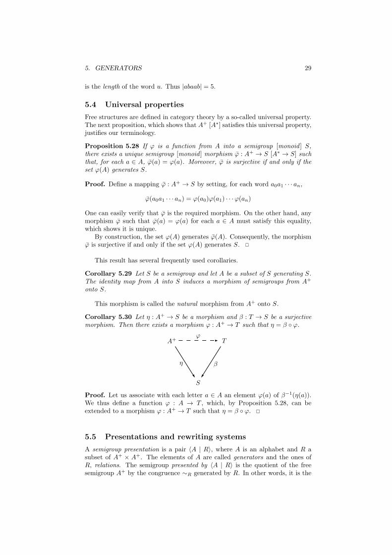
5. GENERATORS 29
is the length of the word u. Thus |abaab| = 5.
5.4 Universal properties
Free structures are defined in category theory by a so-called universal property.The next proposition, which shows that A+ [A∗] satisfies this universal property,justifies our terminology.
Proposition 5.28 If ϕ is a function from A into a semigroup [monoid ] S,there exists a unique semigroup [monoid ] morphism ϕ : A+ → S [A∗ → S] suchthat, for each a ∈ A, ϕ(a) = ϕ(a). Moreover, ϕ is surjective if and only if theset ϕ(A) generates S.
Proof. Define a mapping ϕ : A+ → S by setting, for each word a0a1 · · · an,
ϕ(a0a1 · · · an) = ϕ(a0)ϕ(a1) · · ·ϕ(an)
One can easily verify that ϕ is the required morphism. On the other hand, anymorphism ϕ such that ϕ(a) = ϕ(a) for each a ∈ A must satisfy this equality,which shows it is unique.
By construction, the set ϕ(A) generates ϕ(A). Consequently, the morphismϕ is surjective if and only if the set ϕ(A) generates S.
This result has several frequently used corollaries.
Corollary 5.29 Let S be a semigroup and let A be a subset of S generating S.The identity map from A into S induces a morphism of semigroups from A+
onto S.
This morphism is called the natural morphism from A+ onto S.
Corollary 5.30 Let η : A+ → S be a morphism and β : T → S be a surjectivemorphism. Then there exists a morphism ϕ : A+ → T such that η = β ◦ ϕ.
A+ T
S
η
ϕ
β
Proof. Let us associate with each letter a ∈ A an element ϕ(a) of β−1(η(a)).We thus define a function ϕ : A → T , which, by Proposition 5.28, can beextended to a morphism ϕ : A+ → T such that η = β ◦ ϕ.
5.5 Presentations and rewriting systems
A semigroup presentation is a pair 〈A | R〉, where A is an alphabet and R asubset of A+ × A+. The elements of A are called generators and the ones ofR, relations. The semigroup presented by 〈A | R〉 is the quotient of the freesemigroup A+ by the congruence ∼R generated by R. In other words, it is the

30 CHAPTER II. SEMIGROUPS AND BEYOND
semigroup generated by the set A subject to the relations R. This intuitivemeaning is suggested by the notation. Indeed 〈X〉 traditionally denotes thesemigroup generated by a set X and the vertical bar used as a separator can beinterpreted as “such that”, as in a definition like {n ∈ N | n is prime}.
By extension, a semigroup is said to be defined by a presentation 〈A | R〉 ifit is isomorphic to the semigroup presented by 〈A | R〉. Usually, we write u = vinstead of (u, v) ∈ R.
Monoid presentations are defined analogously by replacing the free semi-group by the free monoid. In particular, relations of the form u = 1 are allowed.
Example 5.1 The monoid presented by 〈{a, b} | ab = ba〉 is isomorphic to theadditive monoid N2.
Example 5.2 The monoid presented by 〈{a, b} | ab = 1〉 is the bicyclic monoiddefined in Section 2.2.
6 Idempotents in finite semigroups
If S is a monogenic semigroup, generated by a single element x, the set S consistsof the successive powers of x. If S is infinite, it is isomorphic to the additivesemigroup of positive integers. If S is finite, there exist integers i, p > 0 suchthat
xi+p = xi.
The minimal i and p with this property are called respectively the index and theperiod of x. The semigroup S then has i+ p− 1 elements and its multiplicativestructure is represented in Figure 6.2.
•x
•x2
•x3 . . . . . . . . . . . .xi+p = xi
•
xi+1
•xi+2
•
xi+p−1•
Figure 6.2. The semigroup generated by x.
The next result is a key property of finite semigroups.
Proposition 6.31 Each element of a finite semigroup has an idempotent power.
Proof. Let i and p be the index and the period of an element x. Observe that,for k > i, xk = xk+p. In particular, if k is a multiple of p, say k = qp, one has
(xk)2 = x2k = xk+qp = xk
and thus xk is idempotent. In fact, it is easy to see that the subsemigroup{xi, . . . , xi+p−1} is isomorphic to the additive group Z/pZ.
Proposition 6.31 has two important consequences.
Corollary 6.32 Every nonempty finite semigroup contains at least one idem-potent.
6. IDEMPOTENTS IN FINITE SEMIGROUPS 31
Proposition 6.33 For each finite semigroup S, there exists an integer ω suchthat, for each s ∈ S, sω is idempotent.
Proof. By Proposition 6.31, every element s of S has an idempotent power sns .Let n be the least common multiple of the ns, for s ∈ S. Then s
n is idempotentfor each s ∈ S.
The least integer ω satisfying the property stated in Proposition 6.33 is calledthe exponent of S.
Here is another elementary property connected with idempotents.
Proposition 6.34 Let S be a finite semigroup and let n = |S|. For everysequence s1, . . . , sn of n elements of S, there exists an index i ∈ {1, . . . , n} andan idempotent e ∈ S such that s1 · · · sie = s1 · · · si.
Proof. Consider the sequence s1, s1s2, . . . , s1 · · · sn. If these elements are alldistinct, the sequence exhausts the elements of S and one of them, say s1 · · · si,is idempotent. The result is thus clear in this case. Otherwise, two elements ofthe sequence are equal, say s1 · · · si and s1 · · · sj with i < j. Then we have
s1 · · · si = s1 · · · si(si+1 · · · sj) = s1 · · · si(si+1 · · · sj)ω
where ω is the exponent of S. The proposition follows, since (si+1 · · · sj)ω isidempotent.
If S is a semigroup and n is a positive integer, we set
Sn = {s1 · · · sn | si ∈ S for 1 6 i 6 n}
Corollary 6.35 Let S be a finite semigroup and let E(S) be the set of idempo-tents of S. Then for every n > |S|, Sn = SE(S)S.
Corollary 6.35 states that every sufficiently long sequence of elements of afinite semigroup contains a subsequence of consecutive elements whose productis idempotent. The proof of this result is elementary and relies mainly on thepigeon-hole principle. We shall now present a more difficult result whose proofrests on a celebrated combinatorial theorem, due to Ramsey, which we shalladmit without proof.
An m-colouring of a set E is a function from E into {1, . . . ,m}. An r-subsetof E is a subset with r elements.
Theorem 6.36 (Ramsey) Let r, k,m be integers satisfying k > r, m > 0.Then there exists an integer N = R(r, k,m) such that for every finite set Ehaving at least N elements and for every m-colouring of the set of the r-subsetsof E, there exists a k-subset of E of which all r-subsets have the same colour.
The next result clearly generalises Proposition 6.34.
Theorem 6.37 For each finite semigroup S, for each k > 0, there exists aninteger N > 0 such that, for every alphabet A, for every morphism ϕ : A+ →S and for every word w of A+ of length greater than or equal to N , thereexists an idempotent e ∈ S and a factorisation w = xu1 · · ·uky with x, y ∈ A∗,u1, . . . , uk ∈ A
+ and ϕ(u1) = . . . = ϕ(uk) = e.

32 CHAPTER II. SEMIGROUPS AND BEYOND
Proof. It suffices to prove the result for k > 2. Put N = R(2, k+1, |S|) and letw be a word of length greater than or equal to N . Let w = a1 · · · aNw
′, wherea1, . . . , aN are letters. We define a colouring of pairs of elements of {1, . . . , N}into |S| colours in the following way: the colour of {i, j}, where i < j, is theelement ϕ(ai · · · aj−1) of S. According to Ramsey’s theorem, one can find k+1indices i0 < i1 < · · · < ik such that all the pairs of elements of {i0, . . . , ik} havethe same colour e. Since we assume k > 2, one has in particular
e = ϕ(ai0) · · ·ϕ(ai1−1) = ϕ(ai1) · · ·ϕ(ai2−1)
= ϕ(ai0) · · ·ϕ(ai1−1)ϕ(ai1) · · ·ϕ(ai2−1) = ee
whereby ee = e. Thus e is idempotent and we obtain the required factori-sation by taking x = a1 · · · ai0−1, uj = aij−1
· · · aij−1 for 1 6 j 6 k andy = aik · · · aNw
′.
There are many quantifiers in the statement of Theorem 6.37, but their orderis important. In particular, the integer N does not depend on the size of A,which can even be infinite.
Proposition 6.38 LetM be a finite monoid and let π : A∗ →M be a surjectivemorphism. For any n > 0, there exists N > 0 and an idempotent e in Msuch that, for any u0, u1, . . . , uN ∈ A∗ there exists a sequence 0 6 i0 < i1 <. . . < in 6 N such that π(ui0ui0+1 · · ·ui1−1) = π(ui1ui1+1 · · ·ui2−1) = . . . =π(uin−1
· · ·uin−1) = e.
Proof. Let N = R(2, n + 1, |M |) and let u0, u1, . . . , uN be words of A∗. LetE = {1, . . . , N}. We define a colouring into |M | colours of the 2-subsets of E inthe following way: the colour of the 2-subset {i, j} (with i < j) is the elementπ(uiui+1 · · ·uj−1) of M . According to Ramsey’s theorem, one can find k + 1indices i0 < i1 < · · · < ik such that all the 2-subsets of {i0, . . . , ik} have thesame colour. In particular, since k > 2, one gets
π(ui0ui0+1 · · ·ui1−1) = π(ui1ui1+1 · · ·ui2−1) = . . . = π(uin−1· · ·uin−1)
= π(ui0ui0+1 · · ·ui2−1)
Let e be the common value of these elements. It follows from the equalitiesπ(ui0ui0+1 · · ·ui1−1) = π(ui1ui1+1 · · ·ui2−1) = π(ui0ui0+1 · · ·ui2−1) that ee = eand thus e is idempotent.
There is also a uniform version of Theorem 6.37, which is more difficult toestablish.
Theorem 6.39 For each finite semigroup S, for each k > 0, there exists aninteger N > 0 such that, for every alphabet A, for every morphism ϕ : A+ → Sand for every word w of A+ of length greater than or equal to N , there existsan idempotent e ∈ S and a factorisation w = xu1 · · ·uky with x, y ∈ A∗, |u1| =. . . = |uk| and ϕ(u1) = . . . = ϕ(uk) = e.
Let us conclude this section with an important combinatorial result of ImreSimon. A factorisation forest is a function F that associates with every word x ofA2A∗ a factorisation F (x) = (x1, . . . , xn) of x such that n > 2 and x1, . . . , xn ∈
7. EXERCISES 33
A+. The integer n is the degree of the factorisation F (x). Given a factorisationforest F , the height function of F is the function h : A∗ → N defined recursivelyby
h(x) =
{0 if |x| 6 1
1 + max {h(xi) | 1 6 i 6 n} if F (x) = (x1, . . . , xn)
The height of F is the least upper bound of the heights of the words of A∗.LetM be a finite monoid and let ϕ : A∗ →M be a morphism. A factorisation
forest F is Ramseyan modulo ϕ if, for every word x of A2A∗, F (x) is either ofdegree 2 or there exists an idempotent e of M such that F (x) = (x1, . . . , xn)and ϕ(x1) = ϕ(x2) = · · · = ϕ(xn) = e for 1 6 i 6 n. The factorisation foresttheorem was first proved by I. Simon in [139, 140, 141] and later improved in[27, 32, 33, 71]:
Theorem 6.40 Let ϕ be a morphism from A∗ into a finite monoid M . Thereexists a factorisation forest of height 6 3|M | − 1 which is Ramseyan modulo ϕ.
Proof. TO DO.
7 Exercises
Section 2
1. Show that, up to isomorphism, there are 5 semigroups of order 2. There arealso 14 semigroups of order 3 and the number of semigroups of order 6 8 isknown to be 1843120128. . .
Section 3
2. Let I and J be ideals of a semigroup S such that I ⊆ J . Show that I is anideal of J , J/I is an ideal of S/I and (S/I)/(J/I) = S/J .
3. Let T be a semigroup and let R and S be subsemigroups of T .
(1) Show that R∪S is a subsemigroup of T if and only if RS ∪SR is a subsetof R ∪ S.
(2) Show that this condition is satisfied if R and S are both left ideals or bothright ideals, or if either R or S is an ideal.
(3) Show that if R is an ideal of T , then S∩R is an ideal of S and (S∪R)/R =S/(S ∩R).
4. (Hickey [57]) Let M be a monoid and let m be an element of M .
(1) Show that the operation ◦ defined on the set mM ∩Mm by
xm ◦my = xmy
is well defined.
(2) Show that (mM ∩Mm, ◦) is a monoid with identity m which divides M .
Section 4
34 CHAPTER II. SEMIGROUPS AND BEYOND
5. Show that, if n > 2, Tn is generated by the three functions a, b, and c of thetable below
1 1 2 3 · · · n− 1 na 2 3 4 · · · n 1b 2 1 3 · · · n− 1 nc 1 2 3 · · · n− 1 1
An element s of Tn is a function from {1, . . . , n} into itself. We define the rankr(s) of s to be | Im(s)| and the defect of s to be n− r(s). For instance, a and bhave rank n and defect 0 and c has rank n− 1 and defect 1.
Show that if s is an element of Tn of defect 1, then a, b and s generate Tn.
6. Let (P, S) be a transformation semigroup. Show that (P, S) divides (P, 1P )×(S1, S).
Section 5
7. Show that the number of words of length n on a k-letter alphabet is kn.
Show that, if k > 2, the number of words of length 6 n is kn+1−1k−1 .
8. Describe the semigroups 〈{a, b} | a2 = a, b2 = b, ab = ba〉 and 〈{a, b} | a2 =a, b2 = b〉.
9. Show that the monoid presented by 〈{a, b} | ab = ba = 1〉 is the group (Z,+).
Section 6
10. Let S be a semigroup. Show that for each idempotent e of S, the sets
eS = {es | s ∈ S}, Se = {se | s ∈ S} and eSe = {ese | s ∈ S}
are subsemigroups of S. The semigroup eSe [eS, Se] is called the [left, right ]local semigroup associated with e. Show that eSe is a monoid with identity e.Prove that an element s of S belongs to eSe [eS, Se] if and only if es = s = se[es = s, se = s]. Show that eSe = eS∩Se. What is the connexion with Exercise4?
Chapter III
Languages and automata
This chapter offers a brief overview of the theory of finite automata and formallanguages.
There are different manners to describe a set of words, or a language. Theconstructive approach consists in giving a collection of basic languages and a setof construction rules to build new languages from previously defined ones. Thedefinition of rational languages is of this type. In the descriptive approach, thewords of a language are characterised by a property: the language of words ofeven length, the set of binary representations of prime numbers are examplesof this approach. The automata approach is a special case of the descriptiveapproach: an automaton reads a word as input and decides whether the word isaccepted or not. The set of words accepted by the automaton defines a language.Another variant of the descriptive approach consists in defining languages bylogical formulas, a point of view further studied in Chapter XVIII.
The first three sections of this chapter review standard definitions on words,rational languages and finite automata. The minimal automaton of a languageis defined in terms of morphisms of automata, which is more precise that justrequiring that the number of states is minimal.
Section 4 gives an overview of standard constructions on automata related tovarious operations on languages: Boolean operations, product, star, quotients,inverses of morphisms.
The main result of Section 5 is Kleene’s theorem, which states that a lan-guage is recognisable if and only if it is rational. Kleene’s theorem is obtainedin two steps. First, we present Glushkov’s algorithm to pass from rational ex-pressions to finite automata. Next, we use linear equations to pass from finiteautomata to rational expressions.
1 Words and languages
1.1 Words
Let u = a0a1 · · · an be a word of A∗. The reversal of u is the word u =anan−1 · · · a0 obtained by reading u from right to left.
A word x ∈ A∗ is a factor of u if x = arar+1 · · · as for some r and s such that0 6 r 6 s 6 n. This amounts to saying that there exist two words v, w ∈ A∗
such that u = vxw. Similarly, x is a left factor, or prefix, of u, if there exists
35

36 CHAPTER III. LANGUAGES AND AUTOMATA
a word w ∈ A∗ such that u = xw and x is a right factor or suffix of u, if thereexists a word v of A∗ such that u = vx.
Example 1.1 If u = abaabba, aba is a prefix, ba is a suffix and abaa, baab arefactors of u. One has |u|a = 4 and |u|b = 3, since u contains four occurrences ofa and three of b.
1.2 Orders on words
The relation “being a prefix of” is an order relation on A∗, called the prefix order.which is partial if A contains at least two letters. There are other interestingorders on the free monoid. We describe two of them, the lexicographic orderand the shortlex order.
Let A be an alphabet and let 6 be a total order on A. The lexicographic orderinduced by 6 is the total order on A∗ used in a dictionary. Formally, it is theorder 6lex on A∗ defined by u 6lex v if and only if u is a prefix of v or u = pau′
and v = pbv′ for some p ∈ A∗, a, b ∈ A with a < b. In the shortlex order, wordsare ordered by length and words of equal length are ordered according to thelexicographic order. Formally, it is the order 6 on A∗ defined by u 6 v if andonly if |u| < |v| or |u| = |v| and u 6lex v.
For instance, if A = {a, b} with a < b, then ababb <lex abba but abba < ababb.The next proposition summarises elementary properties of the shortlex order.The proof is straightforward and omitted.
Proposition 1.1 Let u, v ∈ A∗ and let a, b ∈ A.
(1) If u < v, then au < av and ua < va.
(2) If ua 6 vb, then u 6 v.
An important consequence of Proposition 1.1 is that the shortlex order is stable:if u 6 v, then xuy 6 xvy for all x, y ∈ A∗.
1.3 Languages
Let A be a finite alphabet. Subsets of the free monoid A∗ are called languages.For instance, if A = {a, b}, the sets {aba, babaa, bb} and {anban | n > 0} arelanguages.
Several operations can be defined on languages. The Boolean operationscomprise union, complement (with respect to the set A∗ of all words), intersec-tion and difference. Thus, if L and L′ are languages of A∗, one has:
L ∪ L′ = {u ∈ A∗ | u ∈ L or u ∈ L′}
L ∩ L′ = {u ∈ A∗ | u ∈ L and u ∈ L′}
Lc = A∗ − L = {u ∈ A∗ | u /∈ L}
L− L′ = L ∩ L′c = {u ∈ A∗ | u ∈ L and u /∈ L′}
One can also mention the symmetric difference, defined as follows
L△L′ = (L− L′) ∪ (L′ − L) = (L ∪ L′)− (L ∩ L′)
The concatenation product or simply product of two languages L and L′ is thelanguage
LL′ = {uu′ | u ∈ L and u′ ∈ L′}.

1. WORDS AND LANGUAGES 37
The product is an associative operation on the set of languages, which admitsthe language1 {1} as an identity, since the formula {1}L = L{1} = L holds foreach language L. The product is distributive over union, which means that, forall languages L, L1 and L2, one has
L(L1 ∪ L2) = LL1 ∪ LL2 and (L1 ∪ L2)L = L1L ∪ L2L (1.1)
Therefore the languages over A∗ form a semiring with union as addition andconcatenation product as multiplication. For this reason, it is convenient toreplace the symbol ∪ by + and to let 0 denote the empty language and 1 thelanguage {1}. For instance, (1.1) can be rewritten as L(L1 + L2) = LL1 + LL2
and (L1 + L2)L = L1L + L2L. Another convenient notation is to simply letu denote the language {u}. We shall use freely these conventions without anyfurther warning.
Note that the product is not commutative if the alphabet contains at leasttwo letters. Moreover, it is not distributive over intersection. For instance
(b ∩ ba){a, aa} = 0{a, aa} = 0 but
b{a, aa} ∩ ba{a, aa} = {ba, baa} ∩ {baa, baaa} = baa
The powers of a language can be defined like in any monoid, by setting L0 = 1,L1 = L and by induction, Ln = Ln−1L for all n > 0. The star of a language L,denoted by L∗, is the sum (union) of all the powers of L:
L∗ =∑
n>0
Ln.
The operator L+ is a variant of the star operator, obtained by considering thesum of all nonzero powers of a language:
L+ =∑
n>0
Ln.
Example 1.2 If L = {a, ba} the words of L+, ordered by increasing length,are a, aa, ba, aaa, aba, baa, aaaa, aaba, abaa, baaa, baba, aaaaa, aaaba, aabaa,abaaa, ababa, baaaa, baaba, babaa, etc.
Note that the notation A∗ [A+] is compatible with the definition of the opera-tions L∗ and L+. Also note the following formulas
0∗ = 1, 0+ = 0 and 1∗ = 1 = 1+.
Let L be a language of A∗ and let u be a word of A∗. The left [right ] quotientu−1L [Lu−1] of L by u is defined as follows:
u−1L = {v ∈ A∗ | uv ∈ L} and Lu−1 = {v ∈ A∗ | vu ∈ L}
It is easy to verify that the formula v−1(u−1L) = (uv)−1L and u−1(Lv−1) =(u−1L)v−1 hold for all words u and v of A∗. We also leave as an exercise to the
1 The language {1}, which consists of only one word, the empty word, should not be
confused with the empty language.
38 CHAPTER III. LANGUAGES AND AUTOMATA
reader the following formulas, where a is a letter:
u−1(L1 + L2) = u−1L1 + u−1L2
u−1(L1 − L2) = u−1L1 − u−1L2
u−1(L1 ∩ L2) = u−1L1 ∩ u−1L2
a−1(L1L2) =
{(a−1L1)L2 if 1 /∈ L1,
(a−1L1)L2 + a−1L2 if 1 ∈ L1
a−1L∗ = (a−1L)L∗
Example 1.3 Let A = {a, b} and L = A∗abaA∗. Then
1−1L = L a−1L = A∗abaA∗ + baA∗
b−1L = L (ab)−1L = A∗abaA∗ + aA∗, etc.
More generally, for any subset X of A∗, the left [right] quotient X−1L [LX−1]of L by X is
X−1L =⋃
u∈X
u−1L = {v ∈ A∗ | there exists u ∈ X such that uv ∈ L}
LX−1 =⋃
u∈X
Lu−1 = {v ∈ A∗ | there exists u ∈ X such that vu ∈ L}
One has, for all languages X, Y and L (new exercises. . . )
(X + Y )−1L = X−1L+ Y −1L
(XY )−1L = Y −1(X−1L)
(X∗)−1L = L+ (X∗)−1(X−1L)
To avoid too much parentheses, it is convenient to define precedence orders foroperators on languages, summarised in Table 1.1.
Operator Priority
L∗, Lc, 1
L1L2, X−1L, LX−1 2
L1 + L2, L1 ∩ L2 3
Table 1.1. Operation precedence table.
The unary operators L∗ and Lc have highest priority. The product and quotientshave higher priority than union and intersection.
2 Rational languages
The set of rational (or regular) languages on A∗ is the smallest set of languagesF satisfying the following conditions:
2. RATIONAL LANGUAGES 39
(a) F contains the languages 0 and a for each letter a ∈ A,
(b) F is closed under finite union, product and star (i.e., if L and L′ arelanguages of F , then the languages L+ L′, LL′ and L∗ are also in F).
The set of rational languages of A∗ is denoted by Rat(A∗).This definition calls for a short comment. Indeed, there is a small subtlety
in the definition, since one needs to ensure the existence of a “smallest set”satisfying the preceding conditions. For this, first observe that the set of alllanguages of A∗ satisfies Conditions (a) and (b). Furthermore, the intersectionof all the sets F satisfying Conditions (a) and (b) again satisfies these conditions:the resulting set is by construction the smallest set satisfying (a) and (b).
To obtain a more constructive definition, one can think of the rational lan-guages as a kind of LEGOTM box. The basic LEGO bricks are the emptylanguage and the languages reduced to a single letter and three operators canbe used to build more complex languages: finite union, product and star. Forinstance, it is easy to obtain a language consisting of a single word. If this wordis the empty word, one makes use of the formula 0∗ = 1. For a word a1a2 · · · anof positive length, one observes that
{a1a2 · · · an} = {a1}{a2} · · · {an}.
Finite languages can be expressed as a finite union of singletons. For instance,
{abaaba, ba, baa} = abaaba+ ba+ baa
Consequently, finite languages are rational and the above definition is equivalentwith the following more constructive version:
Proposition 2.2 Let F0 be the set of finite languages of A∗ and, for all n > 0,let Fn+1 be the set of languages that can be written as K + K ′, KK ′ or K∗,where K and K ′ are languages from Fn. Then
F0 ⊆ F1 ⊆ F2 · · ·
and the union of all the sets Fn is the set of rational languages.
Example 2.1 If A = {a, b}, the language (a+ ab+ ba)∗ is a rational language.
Example 2.2 The set L of all words containing a given factor u is rational,since L = A∗uA∗. Similarly, the set P of all words having the word p as a prefixis rational since P = pA∗.
Example 2.3 The set of words of even [odd] length is rational. Indeed, thislanguage can be written as (A2)∗ [(A2)∗A].
A variant of the previous description consists in using rational expressions torepresent rational languages. Rational expressions are formal expressions (likepolynomials in algebra or terms in logic) defined recursively as follows:
(1) 0 and 1 are rational expressions,
(2) for each letter a ∈ A, a is a rational expression,
(3) if e and e′ are rational expressions, then (e+ e′), (ee′) and e∗ are rationalexpressions.

40 CHAPTER III. LANGUAGES AND AUTOMATA
In practice, unnecessary parentheses can be eliminated by applying the prece-dence rules given in Table 1.1. For instance, ((0∗a)(ba)∗ + (bb∗))∗ is a rationalexpression that should formally be written as (((0∗a)(ba)∗) + (bb∗))∗.
The value of a rational expression e, denoted by v(e), is the language rep-resented by e. The symbol 0 represents the empty language, the symbol 1 thelanguage reduced to the empty word, and each symbol a the language {a}. Fi-nally, the operators union, product and star have their natural interpretation.Formally, one has
v(0) = 0
v(1) = 1
v(a) = a for each letter a ∈ A
v((e+ e′)) = v(e) + v(e′)
v((ee′)) = v(e)v(e′)
v(e∗) = (v(e))∗
Beware not to confuse the notions of a rational expression and of a rational lan-guage. In particular, two rational expressions can represent the same language.For instance, the following expressions all represent the set of all words on thealphabet {a, b}.
e1 = (a+ b)∗, e2 = (a∗b)∗a∗, e3 = 1 + (a+ b)(a+ b)∗
The difficulty raised by this example is deeper than it seems. Even if a rationallanguage can be represented by infinitely many different rational expressions,one could expect to have a unique reduced expression, up to a set of simpleidentities like 0 + L = L = L + 0, 1L = L = L1, (L∗)∗ = L∗, L +K = K + Lor L(K + K ′) = LK + LK ′. In fact, one can show there is no finite basis ofidentities for rational expressions: there exist no finite set of identities permit-ting to deduce all identities between rational expressions. Finding a completeinfinite set of identities is already a difficult problem that leads to unexpecteddevelopments involving finite simple groups [34, 70].
We conclude this section by a standard result: rational languages are closedunder morphisms. An extension of this result will be given in Proposition IV.1.1.The proof of this proposition can be found on page 74.
Proposition 2.3 Let ϕ : A∗ → B∗ be a morphism. If L is a rational languageof A∗, then ϕ(L) is a rational language of B∗.
3 Automata
3.1 Finite automata and recognisable languages
A finite automaton is a 5-tuple A = (Q,A,E, I, F ), where Q is a finite set calledthe set of states, A is an alphabet, E is a subset of Q × A × Q, called the setof transitions and I and F are subsets of Q, called respectively the set of initialstates and the set of final states.
It is convenient to represent an automaton by a labelled graph whose verticesare the states of the automaton and the edges represent the transitions. Theinitial [final] states are pictured by incoming [outgoing] arrows.

3. AUTOMATA 41
Example 3.1 Let A = (Q,A,E, I, F ) where Q = {1, 2}, I = {1, 2}, F = {2},A = {a, b} and E = {(1, a, 1), (2, b, 1), (1, a, 2), (2, b, 2)}. This automaton isrepresented in Figure 3.1.
1a 2 b
a
b
Figure 3.1. An automaton.
Two transitions (p, a, q) and (p′, a′, q′) are consecutive if q = p′. A path in theautomaton A is a finite sequence of consecutive transitions
c = (q0, a1, q1), (q1, a2, q2), . . . , (qn−1, an, qn)
also denoted
c : q0a1−→ q1 · · · qn−1
an−→ qn or q0a1···an−−−−−→ qn.
The state q0 is its origin, the state qn its end, the word a1 · · · an is its label andthe integer n is its length. It is also convenient to consider that for each state
q ∈ Q, there is an empty path q1−→ q from q to q labelled by the empty word.
A path in A is called initial if its origin is an initial state and final if its endis a final state. It is successful (or accepting) if it is initial and final.
A state q is accessible if there an initial path ending in q and it is coaccessibleif there is a final path starting in q.
Example 3.2 Consider the automaton represented in Figure 3.1. The path
c : 1a−→ 1
a−→ 2
b−→ 2
b−→ 1
a−→ 2
b−→ 2
is successful, since its end is a final state. However the path
c : 1a−→ 1
a−→ 2
b−→ 2
b−→ 1
a−→ 2
b−→ 1
has the same label, but is not successful, since its end is 1, a nonfinal state.
A word is accepted by the automaton A if it is the label of at least one successfulpath (beware that it can be simultaneously the label of a nonsuccessful path).The language recognised (or accepted) by the automaton A is the set, denotedby L(A), of all the words accepted by A. Two automata are equivalent if theyrecognise the same language.
A language L ⊆ A∗ is recognisable if it is recognised by a finite automaton,that is, if there is a finite automaton A such that L = L(A).
Example 3.3 Consider the automaton represented in Figure 3.2.
1a 2 b
a
b
Figure 3.2. The automaton A.

42 CHAPTER III. LANGUAGES AND AUTOMATA
We let the reader verify that the language accepted by A is aA∗, the set of allwords whose first letter is a.
Example 3.3 is elementary but it already raises some difficulties. In general,deciding whether a given word is accepted or not might be laborious, sincea word might be the label of several paths. The notion of a deterministicautomaton introduced in Section 3.2 permits one to avoid these problems.
We shall see in the Section 4 that the class of recognisable languages ownsmany convenient closure properties. We shall also see that the recognisablelanguages are exactly the rational languages. Before studying these results inmore detail, it is good to realise that there are some nonrecognisable languages.One can establish this result by a simple, but nonconstructive argument (cf.Exercice 15). To get an explicit example, we shall establish a property of therecognisable languages known as the pumping lemma. Although this statementis formally true for any recognisable language, it is only interesting for theinfinite ones.
Proposition 3.4 (Pumping lemma) Let L be a recognisable language. Thenthere is an integer n > 0 such that every word u of L of length greater than orequal to n can be factorised as u = xyz with x, y, z ∈ A∗, |xy| 6 n, y 6= 1 and,for all k > 0, xykz ∈ L.
Proof. Let A = (Q,A,E, I, F ) be an n-state automaton recognising L and let
u = a1 · · · ar be a word of L of length r > n. Let q0a1−→ q1 · · · qr−1
ar−→ qr bea successful path labelled by u. As r > n, there are two integers i and j, withi < j 6 n, such that qi = qj . Therefore, the word ai+1 . . . aj is the label of aloop around qi, represented in Figure 3.3.
q0 q1 qi qj+1 qr
qi+1
a1
. . .ai aj+1
. . .ar
ai+1
ai+2
aj
Figure 3.3. Illustration of the pumping lemma.
Let x = a1 . . . ai, y = ai+1 . . . aj and z = aj+1 . . . ar. Then |xy| 6 n and for allk > 0, one gets xykz ∈ L, since the word xykz is the label of a successful path.
Unfortunately, the pumping lemma does not characterise the recognisablelanguages. In other words, there exist some nonrecognisable languages whichsatisfy the pumping lemma (see Exercice 8). However, in some cases, the pump-ing lemma remains a convenient criterion to show that a language is not recog-nisable. Here is a standard example.
Corollary 3.5 The language {anbn | n > 0} is not recognisable.

3. AUTOMATA 43
Proof. Let L = {anbn | n > 0}. Suppose that L is recognisable. By thepumping lemma, there is an integer n > 0 such that the word anbn can bewritten as anbn = xyz with x, y, z ∈ A∗, |xy| 6 n, y 6= 1 and xy2z ∈ L (as onecan see, we only use a very weak form of the pumping lemma). As |xy| 6 n, theword xy is prefix of an and thus x = ar, y = as and z = atbn, with r+ s+ t = nand s 6= 0.
an bn
x y z
Then xy2z = ara2satbn and since s 6= 0, one has r + 2s+ t 6= n. It follows thatxy2z is not in L, a contradiction. Therefore L is not recognisable.
3.2 Deterministic automata
An automaton A = (Q,A,E, I, F ) is deterministic if I contains exactly oneinitial state and if, for every state q ∈ Q and for every letter a ∈ A, there existsat most one state q′ such that q
a−→ q′ is a transition of E. When it exists, we
let q · a denote this unique state q′. If q− is the unique initial state, we adoptthe notation (Q,A, · , q−, F ) instead of (Q,A,E, {q−}, F ).
Example 3.4 The automaton represented in Figure 3.4 is deterministic.
1 2 3 4 5
b
a b
a
b
b
a
Figure 3.4. A deterministic automaton.
The following result is one of the cornerstones of automata theory. Its proof isbased on the so-called subset construction.
Proposition 3.6 Every finite automaton is equivalent to a deterministic one.
We shall give in Theorem IV.3.20 a purely algebraic proof of this result. Butlet us first present a standard method known as the powerset construction orthe subset construction.Proof. Let A = (Q,A,E, I, F ) be an automaton. Consider the deterministicautomaton D(A) = (P(Q), A, · , I,F) where F = {P ⊆ Q | P ∩F 6= ∅} and, foreach subset P of Q and for each letter a ∈ A,
P · a = {q ∈ Q | there exists p ∈ P such that (p, a, q) ∈ E}
We claim that D(A) is equivalent to A.

44 CHAPTER III. LANGUAGES AND AUTOMATA
If u = a1 · · · an is accepted by A, there is a successful path
c : q0a1−→ q1 · · · qn−1
an−→ qn
The word u also defines a path
I = P0a1−→ P1 · · · Pn−1
an−→ Pn (3.2)
in D(A). Let us show by induction on i that, for 0 6 i 6 n, qi ∈ Pi. Sincec is a successful path, one has q0 ∈ I = P0. Suppose that qi−1 ∈ Pi−1. Then
since qi−1ai−→ qi is a transition, one gets qi ∈ Pi−1 · ai = Pi. For i = n, we get
qn ∈ Pn and since c is a successful path, qn ∈ F . It follows that Pn meets Fand hence Pn ∈ F . Therefore u is accepted by D(A).
Conversely, let u = a1 · · · an be a word accepted by D(A) and let (3.2) thesuccessful path defined by u. Since Pn is a final state, one can choose an elementqn in Pn ∩F . We can now select, for i = n, n− 1, . . . , 1, an element qi−1 of Pi−1
such that qi−1ai−→ qi is a transition in A. Since q0 ∈ I and qn ∈ F , the path
q0a1−→ q1 · · · qn−1
an−→ qn is successful, and thus u is accepted by A. Thisproves the claim and the proposition.
The subset construction converts a nondeterministic n-state automaton intoa deterministic automaton with at most 2n states. One can show that thisbound is tight (see Exercise 10).
Example 3.5 Let A = {a, b}. Starting from the automaton A represented inFigure 3.5, we get the automaton D(A) drawn in Figure 3.6. In practice, itsuffices to compute the accessible states of D(A), which gives the deterministicautomaton shown in Figure 3.7.
1 2 3
a, b
a a, b
Figure 3.5. A nondeterministic automaton.
1
12
13
∅
2
3 23
123
a
ba, b
a, b
a, b
a
b
ba, b
aba
Figure 3.6. After determinisation...

3. AUTOMATA 45
1
12
13
123
a
b
a
b
b
aba
Figure 3.7. . . . and trimming.
3.3 Complete, accessible, coaccessible and trim automata
An automaton A = (Q,A, · , q−, F ) is complete if, for each state q ∈ Q and for
each letter a ∈ A, there is at least one state q′ such that qa−→ q′ is a transition.
Example 3.6 The automaton represented in Figure 3.8 is neither complete, nordeterministic. It is not deterministic, since the transitions (1, a, 1) and (1, a, 2)have the same label and the same origin. It is not complete, since there is notransition of the form 2
a−→ q.
1a 2 b
a
b
Figure 3.8. An incomplete, nondeterministic automaton.
On the other hand, the automaton represented in Figure 3.9 is complete anddeterministic.
1a 2 b
b
a
Figure 3.9. A complete and deterministic automaton.
An automaton is accessible if all its states are accessible. Similarly, it iscoaccessible if all its states are coaccessible. Finally, an automaton is trim if itis simultaneously accessible and coaccessible. It is not difficult to see that everydeterministic automaton is equivalent to a trim one.
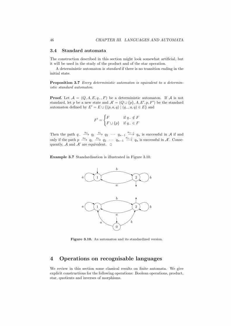
46 CHAPTER III. LANGUAGES AND AUTOMATA
3.4 Standard automata
The construction described in this section might look somewhat artificial, butit will be used in the study of the product and of the star operation.
A deterministic automaton is standard if there is no transition ending in theinitial state.
Proposition 3.7 Every deterministic automaton is equivalent to a determin-istic standard automaton.
Proof. Let A = (Q,A,E, q−, F ) be a deterministic automaton. If A is notstandard, let p be a new state and A′ = (Q ∪ {p}, A,E′, p, F ′) be the standardautomaton defined by E′ = E ∪ {(p, a, q) | (q−, a, q) ∈ E} and
F ′ =
{F if q− /∈ F
F ∪ {p} if q− ∈ F
Then the path q−a0−→ q1
a1−→ q2 · · · qn−1an−1
−→ qn is successful in A if and
only if the path pa0−→ q1
a1−→ q2 · · · qn−1an−1
−→ qn is successful in A′. Conse-quently, A and A′ are equivalent.
Example 3.7 Standardisation is illustrated in Figure 3.10.
1a 2 b
b
a
0
1 2a b
b
a
a b
Figure 3.10. An automaton and its standardized version.
4 Operations on recognisable languages
We review in this section some classical results on finite automata. We giveexplicit constructions for the following operations: Boolean operations, product,star, quotients and inverses of morphisms.

4. OPERATIONS ON RECOGNISABLE LANGUAGES 47
4.1 Boolean operations
We give in this section the well known constructions for union, intersection andcomplement. Complementation is trivial, but requires a deterministic automa-ton.
Proposition 4.8 The union of two recognisable languages is recognisable.
Proof. Let L [L′] be a recognisable language of A∗ recognised by the automatonA = (Q,A,E, I, F ) [A′ = (Q′, A,E′, I ′, F ′)]. We suppose that Q and Q′ aredisjoint sets and thus one can identify E and E′ with subsets of (Q∪Q′)×A×(Q ∪ Q′). Then L + L′ is recognised by the automaton (Q ∪ Q′, A,E ∪ E′, I ∪I ′, F ∪ F ′).
Example 4.1 If L [L′] is recognised by the automaton A [A′] represented inFigure 4.11, then L+ L′ is recognised by the automaton represented in Figure4.12.
1 2
a b
a
1 2
3
ba
a b
Figure 4.11. The automata A and A′.
1 2
a b
a
4 5
6
ba
a b
Figure 4.12. An automaton recognising L+ L′.
Corollary 4.9 Every finite language is recognisable.
Proof. Since recognisable languages are closed under union, it suffices to verifythat the singletons are recognisable. But it is clear that the language a1a2 · · · anis recognised by the automaton represented in Figure 4.13.
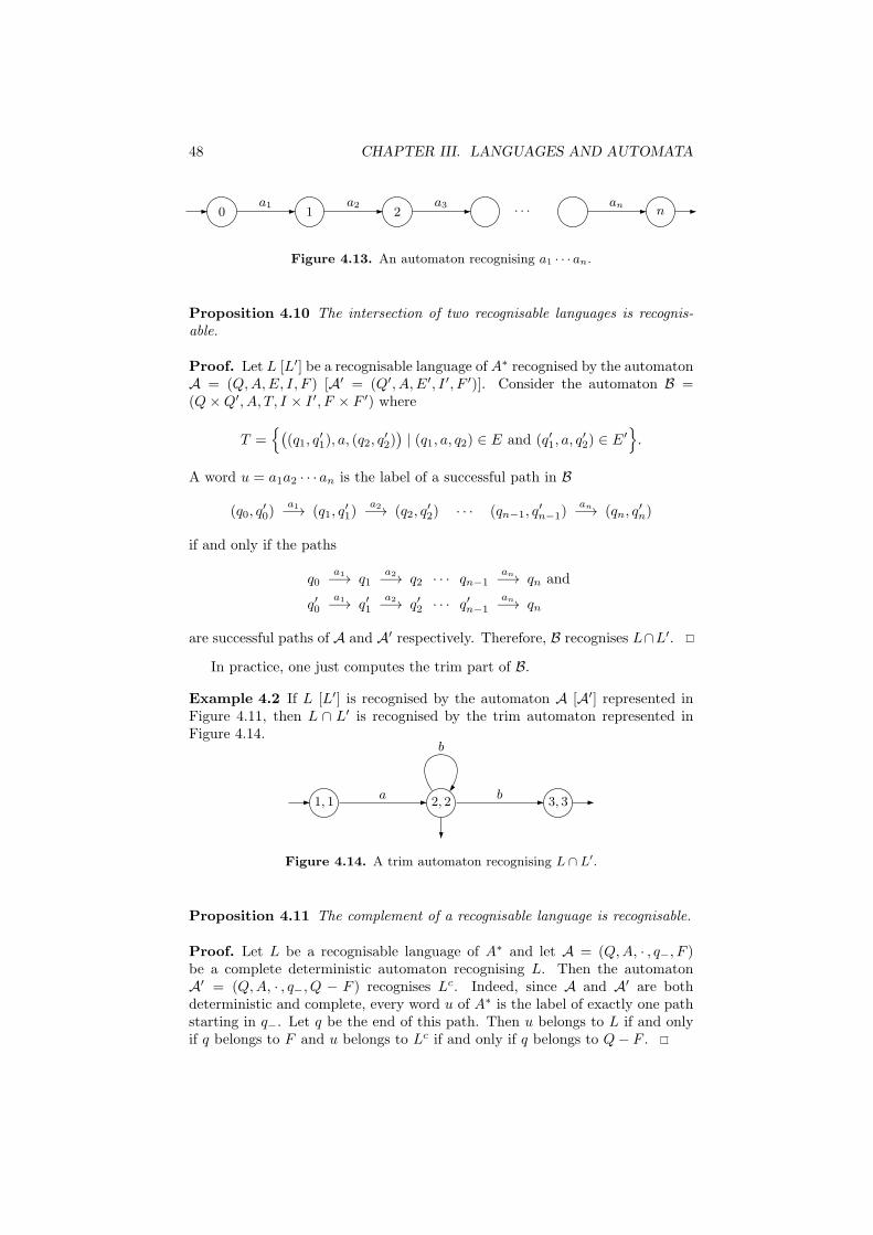
48 CHAPTER III. LANGUAGES AND AUTOMATA
0 1 2 na1 a2 a3 . . . an
Figure 4.13. An automaton recognising a1 · · · an.
Proposition 4.10 The intersection of two recognisable languages is recognis-able.
Proof. Let L [L′] be a recognisable language of A∗ recognised by the automatonA = (Q,A,E, I, F ) [A′ = (Q′, A,E′, I ′, F ′)]. Consider the automaton B =(Q×Q′, A, T, I × I ′, F × F ′) where
T ={(
(q1, q′1), a, (q2, q
′2))| (q1, a, q2) ∈ E and (q′1, a, q
′2) ∈ E
′}.
A word u = a1a2 · · · an is the label of a successful path in B
(q0, q′0)
a1−→ (q1, q′1)
a2−→ (q2, q′2) · · · (qn−1, q
′n−1)
an−→ (qn, q′n)
if and only if the paths
q0a1−→ q1
a2−→ q2 · · · qn−1an−→ qn and
q′0a1−→ q′1
a2−→ q′2 · · · q′n−1
an−→ qn
are successful paths of A and A′ respectively. Therefore, B recognises L∩L′.
In practice, one just computes the trim part of B.
Example 4.2 If L [L′] is recognised by the automaton A [A′] represented inFigure 4.11, then L ∩ L′ is recognised by the trim automaton represented inFigure 4.14.
1, 1 2, 2 3, 3
b
a b
Figure 4.14. A trim automaton recognising L ∩ L′.
Proposition 4.11 The complement of a recognisable language is recognisable.
Proof. Let L be a recognisable language of A∗ and let A = (Q,A, · , q−, F )be a complete deterministic automaton recognising L. Then the automatonA′ = (Q,A, · , q−, Q − F ) recognises Lc. Indeed, since A and A′ are bothdeterministic and complete, every word u of A∗ is the label of exactly one pathstarting in q−. Let q be the end of this path. Then u belongs to L if and onlyif q belongs to F and u belongs to Lc if and only if q belongs to Q− F .
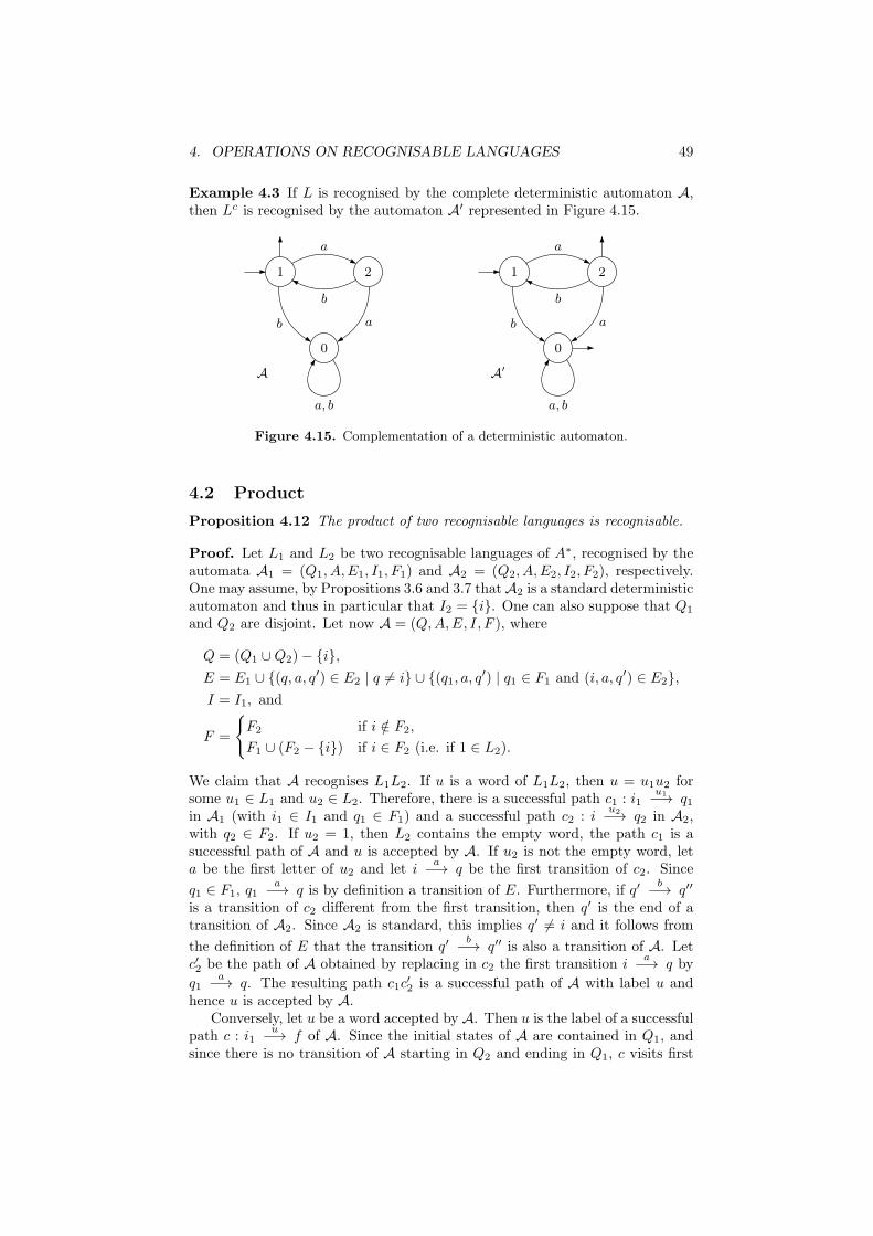
4. OPERATIONS ON RECOGNISABLE LANGUAGES 49
Example 4.3 If L is recognised by the complete deterministic automaton A,then Lc is recognised by the automaton A′ represented in Figure 4.15.
0
1 2
a, b
b
a
b
a
A A′
0
1 2
a, b
b
a
b
a
Figure 4.15. Complementation of a deterministic automaton.
4.2 Product
Proposition 4.12 The product of two recognisable languages is recognisable.
Proof. Let L1 and L2 be two recognisable languages of A∗, recognised by theautomata A1 = (Q1, A,E1, I1, F1) and A2 = (Q2, A,E2, I2, F2), respectively.One may assume, by Propositions 3.6 and 3.7 thatA2 is a standard deterministicautomaton and thus in particular that I2 = {i}. One can also suppose that Q1
and Q2 are disjoint. Let now A = (Q,A,E, I, F ), where
Q = (Q1 ∪Q2)− {i},
E = E1 ∪ {(q, a, q′) ∈ E2 | q 6= i} ∪ {(q1, a, q
′) | q1 ∈ F1 and (i, a, q′) ∈ E2},
I = I1, and
F =
{F2 if i /∈ F2,
F1 ∪ (F2 − {i}) if i ∈ F2 (i.e. if 1 ∈ L2).
We claim that A recognises L1L2. If u is a word of L1L2, then u = u1u2 forsome u1 ∈ L1 and u2 ∈ L2. Therefore, there is a successful path c1 : i1
u1−→ q1in A1 (with i1 ∈ I1 and q1 ∈ F1) and a successful path c2 : i
u2−→ q2 in A2,with q2 ∈ F2. If u2 = 1, then L2 contains the empty word, the path c1 is asuccessful path of A and u is accepted by A. If u2 is not the empty word, leta be the first letter of u2 and let i
a−→ q be the first transition of c2. Since
q1 ∈ F1, q1a−→ q is by definition a transition of E. Furthermore, if q′
b−→ q′′
is a transition of c2 different from the first transition, then q′ is the end of atransition of A2. Since A2 is standard, this implies q′ 6= i and it follows from
the definition of E that the transition q′b−→ q′′ is also a transition of A. Let
c′2 be the path of A obtained by replacing in c2 the first transition ia−→ q by
q1a−→ q. The resulting path c1c
′2 is a successful path of A with label u and
hence u is accepted by A.Conversely, let u be a word accepted by A. Then u is the label of a successful
path c : i1u−→ f of A. Since the initial states of A are contained in Q1, and
since there is no transition of A starting in Q2 and ending in Q1, c visits first

50 CHAPTER III. LANGUAGES AND AUTOMATA
some states of Q1 and then possibly some states of Q2. If all the states visitedby c are in Q1, one has in particular f ∈ Q1. But this is only possible if 1 ∈ L2,and in this case, c is also a successful path of A1, and hence u ∈ L1 ⊆ L1L2.If c visits some states of Q2, then c contains a unique transition of the forme = (q1, a, q2) with q1 ∈ F1 and q2 ∈ Q2. Therefore c = c1ec2, where c1 is apath in A1 and c2 is a path in A2. Denoting by u1 [u2] the label of c1 [c2], weget u = u1au2. Since c1 is a successful path in A1, one has u1 ∈ L1. Moreover,by definition of E, e′ = (i, a, q2) is a transition of A2. Therefore the path e′c2is a successful path in A2 with label au2. It follows that au2 ∈ L2 and thusu ∈ L1L2, proving the claim and the proposition.
Example 4.4 If L1 [L2] is recognised by the automaton A1 [A2] representedin Figure 4.16, then L1L2 is recognised by the automaton represented in Figure4.17.
1 2
3
b
a
ba
A1 A2
1 2 3a
a
a
Figure 4.16. The automata A1 and A2.
1 2
3
b
a
ba
4 5a
a
a
a
Figure 4.17. An automaton recognising L1L2.
4.3 Star
Proposition 4.13 The star of a recognisable language is recognisable.
Proof. Let L be a recognisable language of A∗, recognised by the deterministicstandard automaton A = (Q,A,E, q−, F ). Let A
′ = (Q,A,E′, {q−}, F ∪ {q−})be the nondeterministic automaton defined by
E′ = E ∪ {(q, a, q′) | q ∈ F and (q−, a, q′) ∈ E}.

4. OPERATIONS ON RECOGNISABLE LANGUAGES 51
Let us show that A′ recognises L∗. If u is a word of L∗, then either u is theempty word, which is accepted by A′ since q− is a final state, or u = u1u2 · · ·unwith u1, . . . , un ∈ L − 1. Each ui is the label of a successful path of A, sayci : q−
ui−→ qi with qi ∈ F . Let ai be the first letter of ui and let q−ai−→ pi be
the first transition of ci. Let i ∈ {2, . . . , n}. As qi−1 ∈ F , the definition of E′
shows that qi−1ai−→ pi is a transition of A′. Denote by c′i the path obtained
by replacing in ci the first transition q−ai−→ pi by qi−1
ai−→ pi. This defines,
for 2 6 i 6 n, a path c′i : qi−1ui−→ qi in A′. Therefore, the path c1c
′2 · · · c
′n is a
successful path of label u in A′ and hence u is accepted by A′.Conversely, let u be a word accepted by A′. If u = 1, one has u ∈ L∗.
Otherwise, u is the label of a nonempty successful path c of A′. This path canbe factorised as
c = q−u0−→ q1
a1−→ q′1u1−→ q2
a2−→ q′2 · · · qnan−→ q′n
un−→ qn+1
where the transitions e1 = q1a1−→ q′1, e2 = q2
a2−→ q′2, . . . , en = qnun−→ q′n+1
are exactly the transitions of E′ − E occurring in c. Thus by definition ofE′, one gets, for 1 6 i 6 n, qi ∈ F and e′i = (q−, ai, q
′i) ∈ E. Furthermore,
qn+1 ∈ F ∪ {q−} since c is a successful path. Consequently, the paths
q−ai−→ q′i
ui−→ qi+1
are paths of A. For 1 6 i 6 n − 1, these paths are successful, since qi ∈ F .Moreover, since A is standard2, qn+1 is different from q− and hence qn+1 ∈ F .
Consequently aiui ∈ L for 1 6 i 6 n. Since q−u0−→ q1 is also a successful path
of A, one also has u0 ∈ L, and hence u ∈ L∗.
Example 4.5 If L is recognised by the standard deterministic automaton rep-resented in Figure 4.18, then L∗ is recognised by the nondeterministic automatonrepresented in Figure 4.19.
1 2 3a
a
b
Figure 4.18. A standard automaton recognising L.
1 2 3
a
a
a
b
a
Figure 4.19. An automaton recognising L∗.
2This is the only place where this property is used
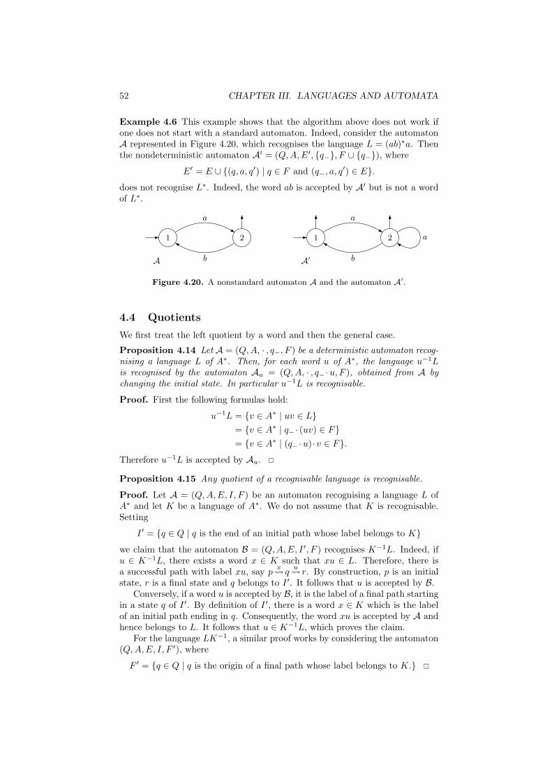
52 CHAPTER III. LANGUAGES AND AUTOMATA
Example 4.6 This example shows that the algorithm above does not work ifone does not start with a standard automaton. Indeed, consider the automatonA represented in Figure 4.20, which recognises the language L = (ab)∗a. Thenthe nondeterministic automaton A′ = (Q,A,E′, {q−}, F ∪ {q−}), where
E′ = E ∪ {(q, a, q′) | q ∈ F and (q−, a, q′) ∈ E}.
does not recognise L∗. Indeed, the word ab is accepted by A′ but is not a wordof L∗.
1 2
a
bA A′
1 2
a
b
a
Figure 4.20. A nonstandard automaton A and the automaton A′.
4.4 Quotients
We first treat the left quotient by a word and then the general case.
Proposition 4.14 Let A = (Q,A, · , q−, F ) be a deterministic automaton recog-nising a language L of A∗. Then, for each word u of A∗, the language u−1Lis recognised by the automaton Au = (Q,A, · , q− ·u, F ), obtained from A bychanging the initial state. In particular u−1L is recognisable.
Proof. First the following formulas hold:
u−1L = {v ∈ A∗ | uv ∈ L}
= {v ∈ A∗ | q− · (uv) ∈ F}
= {v ∈ A∗ | (q− ·u)· v ∈ F}.
Therefore u−1L is accepted by Au.
Proposition 4.15 Any quotient of a recognisable language is recognisable.
Proof. Let A = (Q,A,E, I, F ) be an automaton recognising a language L ofA∗ and let K be a language of A∗. We do not assume that K is recognisable.Setting
I ′ = {q ∈ Q | q is the end of an initial path whose label belongs to K}
we claim that the automaton B = (Q,A,E, I ′, F ) recognises K−1L. Indeed, ifu ∈ K−1L, there exists a word x ∈ K such that xu ∈ L. Therefore, there isa successful path with label xu, say p
x q
u r. By construction, p is an initial
state, r is a final state and q belongs to I ′. It follows that u is accepted by B.Conversely, if a word u is accepted by B, it is the label of a final path starting
in a state q of I ′. By definition of I ′, there is a word x ∈ K which is the labelof an initial path ending in q. Consequently, the word xu is accepted by A andhence belongs to L. It follows that u ∈ K−1L, which proves the claim.
For the language LK−1, a similar proof works by considering the automaton(Q,A,E, I, F ′), where
F ′ = {q ∈ Q | q is the origin of a final path whose label belongs to K.}

4. OPERATIONS ON RECOGNISABLE LANGUAGES 53
4.5 Inverses of morphisms
We now show that recognisable languages are closed under inverses of mor-phisms. A concise proof of an extension of this result will be given in PropositionIV.2.10.
Proposition 4.16 Let ϕ : A∗ → B∗ be a morphism. If L is a recognisablelanguage of B∗, then ϕ−1(L) is a recognisable language of A∗.
Proof. Let B = (Q,B,E, I, F ) be an automaton recognising L. Let A =(Q,A, T, I, F ), where
T = {(p, a, q) | there is a path labelled by ϕ(a) from p to q in B}
We claim that A recognises ϕ−1(L). First, if u is accepted by A, there is asuccessful path of A labelled by u. Consequently, there is a successful path ofB labelled by ϕ(u). Thus ϕ(u) is accepted by B and u ∈ ϕ−1(L).
Let now u = a1 · · · an be a word of ϕ−1(L). Since the word ϕ(u) is acceptedby L, there is a successful path in B labelled by ϕ(u). Let us factorise this pathas
q0ϕ(a1)−− q1 · · · qn−1
ϕ(an)−− qn
These paths define in turn a successful path in A labelled by u:
q0a1−→ q1 · · · qn−1
an−→ qn
which shows that u is accepted by A.
4.6 Minimal automata
Let L be a language of A∗. The Nerode automaton of L is the deterministicautomaton A(L) = (Q,A, · , L, F ) where Q = {u−1L | u ∈ A∗}, F = {u−1L |u ∈ L} and the transition function is defined, for each a ∈ A, by the formula
(u−1L)· a = a−1(u−1L) = (ua)−1L
Beware of this rather abstract definition. Each state of A(L) is a left quotientof L by a word, and hence is a language of A∗. The initial state is the languageL, and the set of final states is the set of all left quotients of L by a word of L.
Proposition 4.17 A language L is recognisable if and only if the set {u−1L |u ∈ A∗} is finite. In this case, L is recognised by its Nerode automaton.
Proof. Let L be a recognisable language, accepted by the deterministic automa-ton A = (Q,A, · , q−, F ). By Proposition 4.14, the language u−1L is acceptedby the automaton Au = (Q,A, · , q− ·u, F ). If n is the number of states of A,there are at most n automata of the form Au and hence at most n distinctlanguages of the form u−1L.
Conversely, if the set {u−1L | u ∈ A∗} is finite, the Nerode automaton of Lis finite and recognises L. Indeed, a word u is accepted by A(L) if and only ifL·u = u−1L is a final state, that is if u ∈ L. It follows that L is recognisable.

54 CHAPTER III. LANGUAGES AND AUTOMATA
Let us define a partial order on deterministic automata as follows. Let A =(Q,A,E, q−, F ) and A′ = (Q′, A,E′, q′−, F
′) be two deterministic automata.Then A′ 6 A if there is a surjective function ϕ : Q→ Q′ such that ϕ(q−) = q′−,ϕ−1(F ′) = F and, for every u ∈ A∗ and q ∈ Q, ϕ(q ·u) = ϕ(q)·u.
Let L be a recognisable language. The next proposition shows that, amongstthe accessible deterministic automata recognising L, the Nerode automaton ofL is minimal for this partial order. For this reason it is called the minimalaccessible automaton of L.
Proposition 4.18 Let A = (Q,A, · , q−, F ) be an accessible and complete de-terministic automaton accepting L. For each state q of Q, let Lq be the languagerecognised by (Q,A, · , q, F ). Then
A(L) = ({Lq | q ∈ Q}, A, · , Lq− , {Lq | q ∈ F}),
where, for all a ∈ A and for all q ∈ Q, Lq · a = Lq·a. Furthermore, the mapq 7→ Lq defines a morphism from A onto A(L).
Proof. Let q be a state of Q. Since q is accessible, there is a word u of A∗ suchthat q− ·u = q, and by Proposition 4.14, one has Lq = u−1L. Conversely, if u isa word, one has u−1L = Lq with q = q− ·u. Therefore
{Lq | q ∈ Q} = {u−1L | u ∈ A∗} and {Lq | q ∈ F} = {u
−1L | u ∈ L}
which proves the first part of the statement.
We claim that the map ϕ : q 7→ Lq defines a morphism from A onto A(L).Indeed, for all a ∈ A, one has
ϕ(q · a) = Lq·a = Lq · a = ϕ(q)· a (4.3)
which proves the claim.
The direct computation of the Nerode automaton is probably the most effi-cient method for a computation by hand, because it directly gives the minimalautomaton. In practice, one starts with the quotient L = 1−1L and one main-tains a table of quotients of L. For each quotient R, it suffices to computethe quotients a−1R for each letter a. These quotients are compared to the ex-isting list of quotients and possibly added to this list. But there is a hiddendifficulty: the comparison of two rational expressions is not always easy since agiven language might be represented by two very different rational expressions.

4. OPERATIONS ON RECOGNISABLE LANGUAGES 55
Example 4.7 For L = (a(ab)∗)∗ ∪ (ba)∗, we get successively:
1−1L = L = L1
a−1L1 = (ab)∗(a(ab)∗)∗ = L2
b−1L1 = a(ba)∗ = L3
a−1L2 = b(ab)∗(a(ab)∗)∗ ∪ (ab)∗(a(ab)∗)∗ = bL2 ∪ L2 = L4
b−1L2 = ∅
a−1L3 = (ba)∗ = L5
b−1L3 = ∅
a−1L4 = a−1(bL2 ∪ L2) = a−1L2 = L4
b−1L4 = b−1(bL2 ∪ L2) = L2 ∪ b−1L2 = L2
a−1L5 = ∅
b−1L5 = a(ba)∗ = L3
which gives the minimal automaton represented in Figure 4.21.
1
2 4
3 5
a
b
a
a
b
a
b
Figure 4.21. The minimal automaton of L.
There are standard algorithms for minimising a given trim deterministic au-tomaton [61] based on the computation of the Nerode equivalence. Let A =(Q,A,E, q−, F ) be a trim deterministic automaton. The Nerode equivalence ∼on Q is defined by p ∼ q if and only if, for every word u ∈ A∗,
p·u ∈ F ⇐⇒ q ·u ∈ F
One can show that ∼ is actually a congruence, which means two things: first,F is saturated by ∼, that is, p ∈ F and p ∼ q implies q ∈ F , and secondly p ∼ qimplies p·x ∼ q ·x for all x ∈ A∗. It follows that there is a well-defined quotientautomaton A/∼ = (Q/∼, A,E, q−, F/∼), where q− is the equivalence class ofq−.
Proposition 4.19 Let A be a trim [and complete] deterministic automaton.Then A/∼ is the minimal [complete] automaton of A.
We shall in particular use the following consequence.

56 CHAPTER III. LANGUAGES AND AUTOMATA
Corollary 4.20 A trim deterministic automaton is minimal if and only if itsNerode equivalence is the identity.
One can show that the operations of completion and of minimisation com-mute. In other words, if A is a trim automaton and if A is its completion, thenthe minimal automaton of A is the completion of the minimal automaton of A.
Example 4.8 The minimal and minimal complete automata of (ab)∗ are givenin Figure 4.22.
1 2
a
b
1 2
0
a
b
b a
a, b
Figure 4.22. The minimal and minimal complete automata of (ab)∗.
Example 4.9 The minimal and minimal complete automata of aA∗b are givenin Figure 4.23.
1 2 3
a b
a
a
b
0 1 2 3
a ba, b
ab
a
b
Figure 4.23. The minimal and minimal complete automata of aA∗b.
5 Rational versus recognisable
5.1 Local languages
A language L of A∗ is said to be local if there exist two subsets P and S of Aand a subset N of A2 such that 3
L− 1 = (PA∗ ∩A∗S)−A∗NA∗.
3P stands for prefix, S for suffix and N for non-factor.

5. RATIONAL VERSUS RECOGNISABLE 57
For instance, if A = {a, b, c}, the language
(abc)∗ = 1 ∪ [(aA∗ ∩A∗c)−A∗{aa, ac, ba, bb, cb, cc)A∗]
is local. The terminology can be explained as follows: in order to check whethera nonempty word belongs to L, it suffices to verify that its first letter is in P , itslast letter is in S and its factors of length 2 are not in N : all these conditions arelocal. Conversely, if a language L is local, it is easy to recover the parametersP , S and N . Indeed, P [S] is the set of first [last] letters of the words of L, andN is the set of words of length 2 that are factors of no word of L.
It is easy to compute a deterministic automaton recognising a local language,given the parameters P , S and N .
Proposition 5.21 Let L = (PA∗ ∩ A∗S) − A∗NA∗ be a local language. ThenL is recognised by the automaton A in which the set of states is A ∪ {1}, theinitial state is 1, the set of final states is S, and the transitions are given by therules 1· a = a if a ∈ P and a· b = b if ab /∈ N .
Proof. Let u = a1 · · · an be a word accepted by A and let
1a1−→ a1
a2−→ a2 · · · an−1an−→ an
be a successful path with label u. Then the state an is final and hence an ∈ S.Similarly, since 1
a1−→ a1 is a transition, one has necessarily a1 ∈ P . Finally,
since for 1 6 i 6 n − 1, aiai+1
−→ ai+1 is a transition, the word aiai+1 is not inN . Consequently, u belongs to L.
Conversely, if u = a1 · · · an ∈ L, one has a1 ∈ P , an ∈ S and, for 1 6 i 6 n,aiai+1 /∈ N . Thus 1
a1−→ a1a2−→ a2 · · · an−1
an−→ an is a successful pathof A and A accepts u. Therefore, the language accepted by A is L.
For a local language containing the empty word, the previous constructioncan be easily modified by taking S ∪ {1} as the set of final states.
Example 5.1 Let A = {a, b, c}, P = {a, b}, S = {a, c} and N = {ab, bc, ca}.Then the automaton in Figure 5.24 recognises the language L = (PA∗∩A∗S)−A∗NA∗.
1
a
b
c
a
b
c
a
b
a
c
b
Figure 5.24. An automaton recognising a local language.

58 CHAPTER III. LANGUAGES AND AUTOMATA
Note also that the automaton A described in Proposition 5.21 has a specialproperty: all the transitions with label a have the same end, namely the statea. More generally, we shall say that a deterministic automaton (not necessarilycomplete) A = (Q,A, · ) is local if, for each letter a, the set {q · a | q ∈ Q} con-tains at most one element. Local languages have the following characterisation:
Proposition 5.22 A rational language is local if and only if it is recognised bya local automaton.
Proof. One direction follows from Proposition 5.21. To prove the oppositedirection, consider a local automaton A = (Q,A, · , q0, F ) recognising a languageL and let
P = {a ∈ A | q0 · a is defined },
S = {a ∈ A | there exists q ∈ Q such that q · a ∈ F},
N = {x ∈ A2 | x is the label of no path in A }
K = (PA∗ ∩A∗S)−A∗NA∗.
Let u = a1 · · · an be a nonempty word of L and let q0a1−→ q1 · · · qn−1
an−→ qnbe a successful path with label u. Necessarily, a1 ∈ P , an ∈ S and, for 1 6 i 6n − 1, aiai+1 /∈ N . Consequently, u ∈ K, which shows that L − 1 is containedin K.
Let now u = a1 · · · an be a nonempty word of K. Then a1 ∈ P , an ∈ S, and,for 1 6 i 6 n−1, aiai+1 /∈ N . Since a1 ∈ P , the state q1 = q0 · a1 is well defined.
Furthermore, since a1a2 /∈ N , a1a2 is the label of some path p0a1−→ p1
a2−→ p2in A. But since A is a local automaton, q0 · a1 = p0 · a1. It follows that the worda1a2 is also the label of the path q0
a1−→ p1a2−→ p2. One can show in the same
way by induction that there exists a sequence of states pi (0 6 i 6 n) such that
aiai+1 is the label of a path pi−1ai−→ pi
ai+1
−→ pi+1 of A. Finally, since an ∈ S,there is a state q such that q · an ∈ F . But since A is a local automaton, one hasq · an = pn−1 · an = pn, whence pn ∈ F . Therefore q0
a1−→ p1 · · · pn−1an−→ pn
is a successful path in A and its label u is accepted by A. Thus K = L− 1.
Local languages are stable under various operations:
Proposition 5.23 Let A1 and A2 be two disjoint subsets of the alphabet A andlet L1 ⊆ A∗
1 and L2 ⊆ A∗2 be two local languages. Then the languages L1 + L2
and L1L2 are local languages.
Proof. Let A1 [A2] be a local automaton recognising L1 [L2]. The proofs ofPropositions 4.8 and 4.12 give an automaton recognising L1 + L2 and L1L2. Asimple verification shows that these constructions produce a local automatonwhen A1 and A2 are local.
Proposition 5.24 Let L be a local language. Then the language L∗ is a locallanguage.
Proof. Let A be a local automaton recognising L. The proof of Proposition4.13 gives an automaton recognising L∗. A simple verification shows that thisconstruction produces a local automaton when A is local.
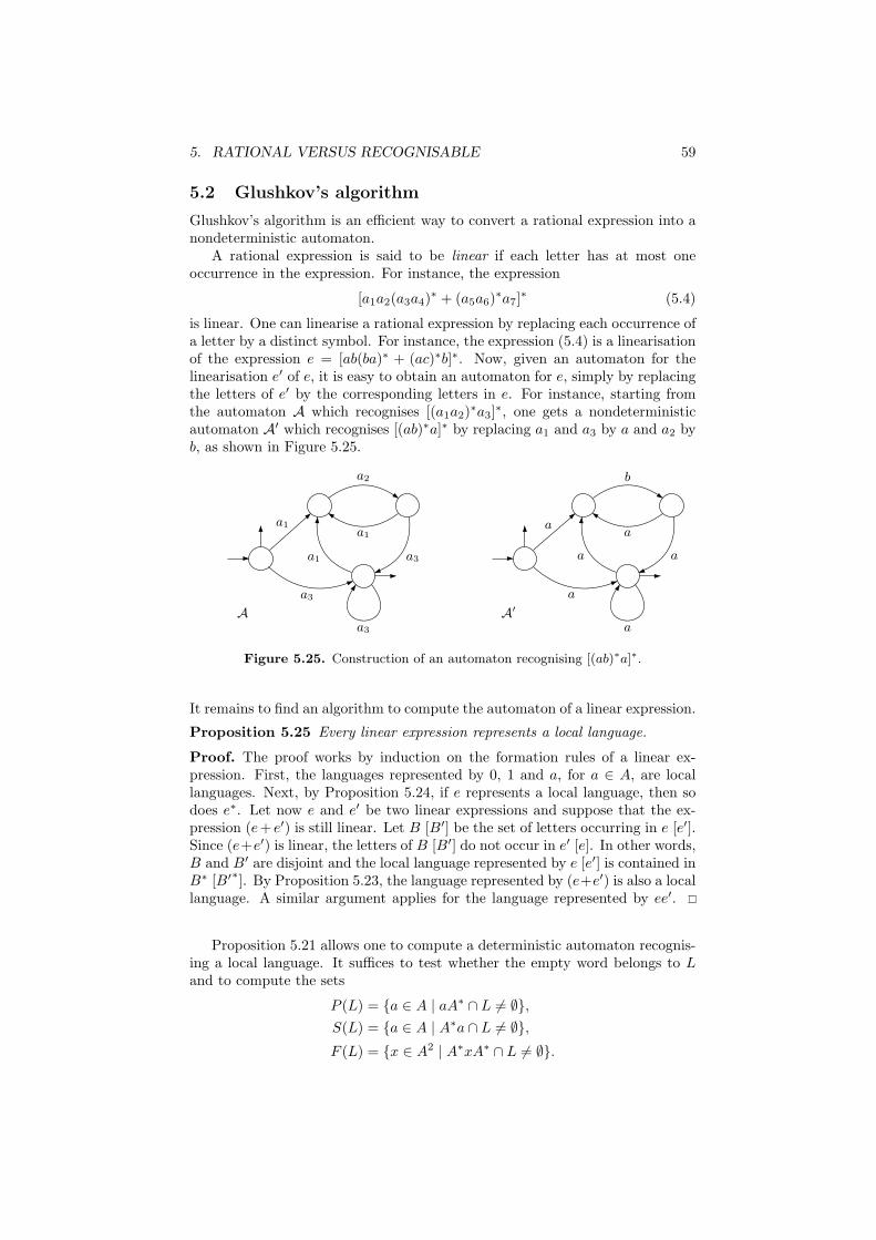
5. RATIONAL VERSUS RECOGNISABLE 59
5.2 Glushkov’s algorithm
Glushkov’s algorithm is an efficient way to convert a rational expression into anondeterministic automaton.
A rational expression is said to be linear if each letter has at most oneoccurrence in the expression. For instance, the expression
[a1a2(a3a4)∗ + (a5a6)
∗a7]∗ (5.4)
is linear. One can linearise a rational expression by replacing each occurrence ofa letter by a distinct symbol. For instance, the expression (5.4) is a linearisationof the expression e = [ab(ba)∗ + (ac)∗b]∗. Now, given an automaton for thelinearisation e′ of e, it is easy to obtain an automaton for e, simply by replacingthe letters of e′ by the corresponding letters in e. For instance, starting fromthe automaton A which recognises [(a1a2)
∗a3]∗, one gets a nondeterministic
automaton A′ which recognises [(ab)∗a]∗ by replacing a1 and a3 by a and a2 byb, as shown in Figure 5.25.
a3
a1
a2
a1
a1 a3
a3
A A′
a
a
b
a
a a
a
Figure 5.25. Construction of an automaton recognising [(ab)∗a]∗.
It remains to find an algorithm to compute the automaton of a linear expression.
Proposition 5.25 Every linear expression represents a local language.
Proof. The proof works by induction on the formation rules of a linear ex-pression. First, the languages represented by 0, 1 and a, for a ∈ A, are locallanguages. Next, by Proposition 5.24, if e represents a local language, then sodoes e∗. Let now e and e′ be two linear expressions and suppose that the ex-pression (e+ e′) is still linear. Let B [B′] be the set of letters occurring in e [e′].Since (e+e′) is linear, the letters of B [B′] do not occur in e′ [e]. In other words,B and B′ are disjoint and the local language represented by e [e′] is contained inB∗ [B′∗]. By Proposition 5.23, the language represented by (e+e′) is also a locallanguage. A similar argument applies for the language represented by ee′.
Proposition 5.21 allows one to compute a deterministic automaton recognis-ing a local language. It suffices to test whether the empty word belongs to Land to compute the sets
P (L) = {a ∈ A | aA∗ ∩ L 6= ∅},
S(L) = {a ∈ A | A∗a ∩ L 6= ∅},
F (L) = {x ∈ A2 | A∗xA∗ ∩ L 6= ∅}.
60 CHAPTER III. LANGUAGES AND AUTOMATA
This can be done by recursion, given a linear rational expression representingthe language. We first execute the procedure
EmptyWord(e: linear expression): boolean;
which determines whether the empty word belongs to the language representedby e.
EmptyWord(0) = false;EmptyWord(1) = true;EmptyWord(a) = false for all a ∈ A;EmptyWord(e+ e′) = EmptyWord(e) or EmptyWord(e′);EmptyWord(e· e′) = EmptyWord(e) and EmptyWord(e′);EmptyWord(e∗) = true;
Now P , S and F are computed by the following recursive procedures:
P(0) = ∅; S(0) = ∅;P(1) = ∅; S(1) = ∅;P(a) = {a} for all a ∈ A; S(a) = {a} for all a ∈ A;P(e+ e′) = P(e) ∪ P(e′); S(e+ e′) = S(e) ∪ S(e′);if EmptyWord(e) if EmptyWord(e′)then P(e· e′) = P(e) ∪ P(e′) then S(e· e′) = S(e) ∪ S(e′)else P (e· e′) = P (e); else S(e· e′) = S(e′);
P(e∗) = P(e); S(e∗) = S(e);
F(0) = ∅;F(1) = ∅;F(a) = ∅ for all a ∈ A;F(e+ e′) = F(e) ∪ F(e′);F(e· e′) = F(e) ∪ F(e′) ∪ S(e)P(e′);F(e∗) = F(e) ∪ S(e)P(e);
In summary, Glushkov’s algorithm to convert a rational expression e into anondeterministic automaton works as follows:
(1) Linearise e into e′ and memorise the coding of the letters.
(2) Compute recursively the sets P (e′), S(e′) and F (e′). Then compute adeterministic automaton A′ recognising e′.
(3) Convert A′ into a nondeterministic automaton A recognising e.
Example 5.2 Consider the rational expression e = (a(ab)∗)∗ + (ba)∗. We firstlinearise e into e′ = (a1(a2a3)
∗)∗ + (a4a5)∗. Let L = L(e) and L′ = L(e′). To
compute the sets P , S and F , one can either use the above-mentioned recursiveprocedures, or proceed to a direct computation (this method is usually preferredin a computation by hand...). Recall that P [S] is the set of first [last] lettersof the words of L′. We get
P = {a1, a4} and S = {a1, a3, a5}
Note that a1 belongs to S since a1 is a word of L′.Next we compute the set F of all words of length 2 that are factors of some
word of L′. We get F = {a1a2, a1a1, a2a3, a3a1, a3a2, a4a5, a5a4}. For instance,a3a1 is a factor of a1a2a3a1 and a3a2 is a factor of a1a2a3a2a3. Since the empty
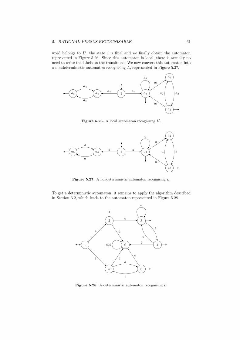
5. RATIONAL VERSUS RECOGNISABLE 61
word belongs to L′, the state 1 is final and we finally obtain the automatonrepresented in Figure 5.26. Since this automaton is local, there is actually noneed to write the labels on the transitions. We now convert this automaton intoa nondeterministic automaton recognising L, represented in Figure 5.27.
1 a1
a2
a3
a4a5
a1
a1a4
a2
a1
a3a2
a5
a4
Figure 5.26. A local automaton recognising L′.
1 a1
a2
a3
a4a5
a
ab
a
a
ba
a
b
Figure 5.27. A nondeterministic automaton recognising L.
To get a deterministic automaton, it remains to apply the algorithm describedin Section 3.2, which leads to the automaton represented in Figure 5.28.
1
2
0 4
5 6
3
a
b
a
b
b
ba
a, b
a
b
a
a
b
Figure 5.28. A deterministic automaton recognising L.

62 CHAPTER III. LANGUAGES AND AUTOMATA
5.3 Linear equations
In this section, we give an algorithm to convert an automaton into a rationalexpression. The algorithm amounts to solving a system of linear equations onlanguages. We first consider an equation of the form
X = KX + L, (5.5)
where K and L are languages and X is the unknown. When K does not containthe empty word, the equation admits a unique solution.
Proposition 5.26 (Arden’s Lemma) If K does not contain the empty word,then X = K∗L is the unique solution of the equation X = KX + L.
Proof. Replacing X by K∗L in the expression KX + L, one gets
K(K∗L) + L = K+L+ L = (K+ + 1)L = K∗L,
and hence X = K∗L is a solution of (5.5). To prove uniqueness, consider twosolutions X1 and X2 of (5.5). By symmetry, it suffices to show that each wordu of X1 also belongs to X2. Let us prove this result by induction on the lengthof u.
If |u| = 0, u is the empty word and if u ∈ X1 = KX1 + L, then necessarilyu ∈ L since 1 /∈ K. But in this case, u ∈ KX2+L = X2. For the induction step,consider a word u of X1 of length n+1. Since X1 = KX1 +L, u belongs eitherto L or to KX1. If u ∈ L, then u ∈ KX2 + L = X2. If u ∈ KX1 then u = kxfor some k ∈ K and x ∈ X1. Since k is not the empty word, one has necessarily|x| 6 n and hence by induction x ∈ X2. It follows that u ∈ KX2 and finallyu ∈ X2. This concludes the induction and the proof of the proposition.
If K contains the empty word, uniqueness is lost.
Proposition 5.27 If K contains the empty word, the solutions of (5.5) are thelanguages of the form K∗M with L ⊆M .
Proof. Since K contains the empty word, one has K+ = K∗. If L ⊆ M , onehas L ⊆M ⊆ K∗M . It follows that the language K∗M is solution of (5.5) since
K(K∗M) + L = K+M + L = K∗M + L = K∗M.
Conversely, let X be a solution of (5.5). Then L ⊆ X and KX ⊆ X. Conse-quently, K2X ⊆ KX ⊆ X and by induction, KnX ⊆ X for all n. It followsthat K∗X =
∑n>0X
nK ⊆ X. The language X can thus be written as K∗Mwith L ⊆M : it suffices to take M = X.
In particular, if K contains the empty word, then A∗ is the maximal solutionof (5.5) and the minimal solution is K∗L.
Consider now a system of the form
X1 = K1,1X1 +K1,2X2 + · · ·+K1,nXn + L1
X2 = K2,1X1 +K2,2X2 + · · ·+K2,nXn + L2
......
Xn = Kn,1X1 +Kn,2X2 + · · ·+Kn,nXn + Ln
(5.6)
We shall only consider the case when the system admits a unique solution.

5. RATIONAL VERSUS RECOGNISABLE 63
Proposition 5.28 If, for 1 6 i, j 6 n, the languages Ki,j do not contain theempty word, the system (5.6) admits a unique solution. If further the Ki,j
and the Li are rational languages, then the solutions Xi of (5.6) are rationallanguages.
Proof. The case n = 1 is handled by Proposition 5.26. Suppose that n > 1.Consider the last equation of the system (5.6), which can be written
Xn = Kn,nXn + (Kn,1X1 + · · ·+Kn,n−1Xn−1 + Ln)
According to Proposition 5.26, the unique solution of this equation is
Xn = K∗n,n(Kn,1X1 + · · ·+Kn,n−1Xn−1 + Ln)
Replacing Xn by this expression in the n−1 first equations, we obtain a systemof n− 1 equations with n− 1 unknowns and one can conclude by induction.
We shall now associate a system of linear equations with every finite au-tomaton A = (Q,A,E, I, F ). Let us set, for p, q ∈ Q,
Kp,q = {a ∈ A | (p, a, q) ∈ E}
Lq =
{1 if q ∈ F
0 if q /∈ F
The solutions of the system defined by these parameters are the languages recog-nised by the automata
Aq = (Q,A,E, {q}, F )
More precisely, we get the following result:
Proposition 5.29 The system (5.6) admits a unique solution (Rq)q∈Q, givenby the formula
Rq = {u ∈ A∗ | there is a path with label u from q to F}
Moreover, the language recognised by A is∑
q∈I Rq.
Proof. Since the languages Kp,q do not contain the empty word, Proposition5.28 shows that the system (5.6) admits a unique solution. It remains to verifythat the family (Rq)q∈Q is a solution of the system, that is, it satisfies for allq ∈ Q the formula
Rq = Kq,1R1 +Kq,2R2 + · · ·+Kq,nRn + Lq (5.7)
Let Sq denote the right-hand side of (5.7). If u ∈ Rq, then u is by definitionthe label of a path from q to a final state f . If u is the empty word, one hasnecessarily q = f and hence Lq = 1. Thus u ∈ Sq in this case. Otherwise,let (q, a, q′) be the first transition of the path. One has u = au′, where u′ isthe label of a path from q′ to f . Then one has a ∈ Kq,q′ , u
′ ∈ Rq′ and finallyu ∈ Sq.
Conversely, let u ∈ Sq. If u = 1, one has necessarily u ∈ Lq, whence q ∈ Fand u ∈ Rq. Otherwise there is a state q′ such that u ∈ Kq,q′Rq′ . Therefore,

64 CHAPTER III. LANGUAGES AND AUTOMATA
u = au′ for some a ∈ Kq,q′ and u′ ∈ Rq′ . On the one hand, (q, a, q′) is atransition of A by definition of Kq,q′ and on the other hand u′ is the label of afinal path starting in q′. The composition of these paths gives a final path withlabel u starting in q. Therefore u ∈ Rq and thus Rq = Sq.
Example 5.3
1 2
3
b
a
a
b a
Figure 5.29. An automaton.
For the automaton represented in Figure 5.29, the system can be written
X1 = aX2 + bX3
X2 = aX1 + bX3 + 1
X3 = aX2 + 1
Substituting aX2 + 1 for X3, one gets the equivalent system
X1 = aX2 + b(aX2 + 1) = (a+ ba)X2 + b
X2 = aX1 + b(aX2 + 1) + 1 = aX1 + baX2 + (b+ 1)
X3 = aX2 + 1
Substituting (a+ ba)X2 + b for X1, one gets a third equivalent system
X1 = (a+ ba)X2 + b
X2 = a((a+ ba)X2 + b) + baX2 + (b+ 1) = (aa+ aba+ ba)X2 + (ab+ b+ 1)
X3 = aX2 + 1
The solution of the second equation is
X2 = (aa+ aba+ ba)∗(ab+ b+ 1)
Replacing X2 by its value in the two other equations, we obtain
X1 = (a+ba)(aa+aba+ba)∗(ab+b+1)+b and X3 = a(aa+aba+ba)∗(ab+b+1)+1
Finally, the language recognised by the automaton is
X1 = (a+ ba)(aa+ aba+ ba)∗(ab+ b+ 1) + b
since 1 is the unique initial state.
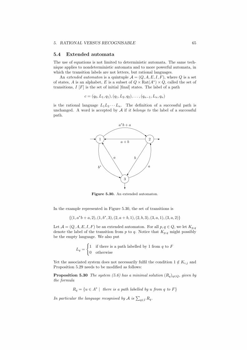
5. RATIONAL VERSUS RECOGNISABLE 65
5.4 Extended automata
The use of equations is not limited to deterministic automata. The same tech-nique applies to nondeterministic automata and to more powerful automata, inwhich the transition labels are not letters, but rational languages.
An extended automaton is a quintuple A = (Q,A,E, I, F ), where Q is a setof states, A is an alphabet, E is a subset of Q× Rat(A∗)×Q, called the set oftransitions, I [F ] is the set of initial [final] states. The label of a path
c = (q0, L1, q1), (q1, L2, q2), . . . , (qn−1, Ln, qn)
is the rational language L1L2 · · ·Ln. The definition of a successful path isunchanged. A word is accepted by A if it belongs to the label of a successfulpath.
1 2
3
a+ b
ba
a∗b+ a
b∗ a
Figure 5.30. An extended automaton.
In the example represented in Figure 5.30, the set of transitions is
{(1, a∗b+ a, 2), (1, b∗, 3), (2, a+ b, 1), (2, b, 3), (3, a, 1), (3, a, 2)}
Let A = (Q,A,E, I, F ) be an extended automaton. For all p, q ∈ Q, we let Kp,q
denote the label of the transition from p to q. Notice that Kp,q might possiblybe the empty language. We also put
Lq =
{1 if there is a path labelled by 1 from q to F
0 otherwise
Yet the associated system does not necessarily fulfil the condition 1 /∈ Ki,j andProposition 5.29 needs to be modified as follows:
Proposition 5.30 The system (5.6) has a minimal solution (Rq)q∈Q, given bythe formula
Rq = {u ∈ A∗ | there is a path labelled by u from q to F}
In particular the language recognised by A is∑
q∈I Rq.

66 CHAPTER III. LANGUAGES AND AUTOMATA
Proof. Let us first verify that the family (Rq)q∈Q is indeed a solution of (5.6),i.e. it satisfies, for all q ∈ Q:
Rq = Kq,1R1 +Kq,2R2 + · · ·+Kq,nRn + Lq (5.8)
Denote by Sq the right-hand side of (5.8). If u ∈ Rq, then u is by definitionthe label of a path from q to F . If u = 1, one has Lq = 1 and thus u ∈ Sq.Otherwise, let (q, u1, q
′) be the first transition of the path. One has u = u1u′,
where u′ is the label of a path from q′ to F . Therefore u1 ∈ Kq,q′ , u′ ∈ Rq′ and
finally u ∈ Sq.Conversely, let u ∈ Sq. If u = 1, one has necessarily u ∈ Lq, whence q ∈ F
and u ∈ Rq. Otherwise, there is a state q′ such that u ∈ Kq,q′Rq′ . Thusu = u1u
′ for some u1 ∈ Kq,q′ and u′ ∈ Rq′ . On the one hand, (q, u1, q′) is a
transition of A by the definition of Kq,q′ and on the other hand, u′ is the labelof a path from q′ to F . Therefore u = u1u
′ is the label of a path from q to Fand u ∈ Rq. Consequently Rq = Sq.
It remains to verify that if (Xq)q∈Q is a solution of the system, then Rq ⊆ Xq
for all q ∈ Q. If u ∈ Rq, there exists a path labelled by u from q to F :
(q0, u1, q1)(q1, u2, q2) · · · (qr−1, ur, qr)
with q0 = q, qr ∈ F , ui ∈ Kqi−1,qi and u1u2 · · ·ur = u. Let us show by inductionon r − i that ui+1 · · ·ur belongs to Xqi . By hypothesis, the Xq are solutions of
Xq = Kq,1X1 +Kq,2X2 + · · ·+Kq,nXn + Lq
In particular, since qr ∈ F , one has 1 ∈ Lqr and hence 1 ∈ Xqr , which givesthe result for r − i = 0. Furthermore, if ui+1 · · ·ur is an element of Xqi , theinclusion Kqi−1,qiXqi ⊆ Xqi−1
shows that uiui+1 · · ·ur is an element of Xqi−1,
which concludes the induction. In particular, u = u1 · · ·ur ∈ Xq.
Example 5.4 For the extended automaton represented in Figure 5.30, the sys-tem can be written
X1 = (a∗b+ a)X2 + b∗X3
X2 = (a+ b)X1 + bX3 + 1
X3 = aX1 + aX2 + 1
Replacing X3 by aX1 + aX2 + 1, and observing that a + b∗a = b∗a, we obtainthe equivalent system
X1 = (a∗b+ a)X2 + b∗(aX1 + aX2 + 1) = b∗aX1 + (a∗b+ b∗a)X2 + b∗
X2 = (a+ b)X1 + b(aX1 + aX2 + 1) + 1 = (a+ b+ ba)X1 + baX2 + b+ 1
X3 = aX1 + aX2 + 1
We deduce from the second equation
X2 = (ba)∗((a+ b+ ba)X1 + b+ 1)
and replacing X2 by its value in the first equation, we obtain
X1 = b∗aX1 + (a∗b+ b∗a)(ba)∗((a+ b+ ba)X1 + b+ 1) + b∗
= (b∗a+ (a∗b+ b∗a)(ba)∗(a+ b+ ba))X1 + (a∗b+ b∗a)(ba)∗(b+ 1) + b∗
5. RATIONAL VERSUS RECOGNISABLE 67
Finally, the language recognised by the automaton is
X1 =(b∗a+ (a∗b+ b∗a)(ba)∗(a+ b+ ba)
)∗[(a∗b+ b∗a)(ba)∗(b+ 1) + b∗]
since 1 is the unique initial state.
5.5 Kleene’s theorem
We are now ready to state the most important result of automata theory.
Theorem 5.31 (Kleene) A language is rational if and only if it is recognis-able.
Proof. It follows from Proposition 5.29 that every recognisable language is ra-tional. Corollary 4.9 states that every finite language is recognisable. Fur-thermore, Propositions 4.8, 4.12 and 4.13 show that recognisable languagesare closed under union, product and star. Thus every rational language isrecognisable.
The following corollary is now a consequence of Propositions 2.3, 4.8, 4.10,4.11, 4.12, 4.13, 4.15 and 4.16.
Corollary 5.32 Recognisable [rational ] languages are closed under Boolean op-erations, product, star, quotients, morphisms and inverses of morphisms.
We conclude this section by proving some elementary decidability resultson recognisable languages. Recall that a property is decidable if there is analgorithm to check whether this property holds or not. We shall also often usethe expressions “given a recognisable language L” or “given a rational languageL”. As long as only decidability is concerned, it makes no difference to givea language by a nondeterministic automaton, a deterministic automaton or aregular expression, since there are algorithms to convert one of the forms into theother. However, the chosen representation is important for complexity issues,which will not be discussed here.
Theorem 5.33 Given a recognisable language L, the following properties aredecidable:
(1) whether a given word belongs to L,
(2) whether L is empty,
(3) whether L is finite,
(4) whether L is infinite,
Proof. We may assume that L is given by a trim deterministic automatonA = (Q,A, · , q−, F ).
(1) To test whether u ∈ L, it suffices to compute q− ·u. If q− ·u ∈ F , thenu ∈ L; if q− ·u /∈ F , or if q− ·u is undefined, then u /∈ L.
(2) Let us show that L is empty if and only if F = ∅. The condition F = ∅is clearly sufficient. Since A is trim, every state of A is accessible. Now, if Ahas at least one final state q, there is a word u such that q− ·u = q. Thereforeu ∈ L and L is nonempty.
(3) and (4). Let us show that L is finite if and only if A does not contain
any loop. If A contains a loop qu−→ q, then L is infinite: indeed, since A
68 CHAPTER III. LANGUAGES AND AUTOMATA
is trim, there exist paths q−x−→ q and q
y−→ f , where f is a final state and
thus L contains all the words xuny. Conversely, if L is infinite, the proof ofthe pumping lemma shows that A contains a loop. Now, checking whether anautomaton contains a loop is easy. Consider the directed graph G obtained fromA by removing all the labels. Then A is loop-free if and only if G is acyclic,a property that can be checked by standard algorithms. One can for instancecompute the transitive closure G′ of G and check whether G′ contains an edgeof the form (q, q).
We leave as an exercise to the reader to prove that the inclusion problemand the equality problem are decidable for two given recognisable languages.
6 Exercises
Section 1
1. Let us say that two words x and y are powers of the same word if there existsa word z and two nonnegative integers n and m such that x = zn and y = zm.Show that two words commute if and only if they are powers of the same word.
2. Two words x and y are conjugate if there exist two words u and v such thatx = uv and y = vu.
(1) Show that two words are conjugate if and only if there exists a word zsuch that xz = zy.
(2) Conclude that the conjugacy relation is an equivalence relation.
3. A word u is a subword of v if v can be written as
v = v0u1v1u2v2 · · ·ukvk
where ui and vi are words (possibly empty) such that u1u2 · · ·uk = u. Forinstance, the words baba and acab are subwords of abcacbab.
(1) Show that the subword relation is a partial ordering on A∗.
(2) (Difficult) Prove that if A is finite, any infinite set of words contains twowords, one of which is a subword of the other.
Section 2
4. Simplify the following rational expressions
(1) ((abb)∗)∗,
(2) a∗b+ a∗ba∗,
(3) 0∗ab1∗,
(4) (a∗b)∗a∗.
5. Let e, e1, e2, e3 be four rational expressions. Verify that the following pairsof rational expressions represent the same language:
(1) e1 + e2 and e2 + e1,
(2) ((e1 + e2) + e3) and (e1 + (e2 + e3)),
(3) ((e1e2)e3) and (e1(e2e3)),
6. EXERCISES 69
(4) (e1(e2 + e3)) and ((e1e2) + (e1e3)),
(5) ((e1 + e2)e3) and ((e1e3) + (e2e3)),
(6) e∗∗ and e∗,
(7) 0 + e and e,
(8) 1e and e,
(9) 0∗ and 1,
(10) (e1 + e2)∗ and (e∗1e2)
∗e∗1.
Section 3
6. A well-parenthesised word is a word on the alphabet {(, )} containing asmany left parenthesises as right parenthesises and such that each of its prefixescontains at least as many left parenthesises as right parenthesises. For instance,((()())()) is a well-parenthesised word, but ((()()))()) is not.
Prove that the language of all well parenthesised words is not recognisable.
7. Prove that the following languages are not recognisable:
(1) {u ∈ {a, b}∗ | |u|a = |u|b},
(2) {anbm | n,m > 0 and n = 2m},
(3) {u ∈ A∗ | u = u}
(4) {vvw | v, w ∈ {a, b}+}
(5) {u ∈ a∗ | |u| is a prime number }
8. Let A = {a, b, c}. Show that the language
L = {(ab)ncn | n > 0}+A∗bbA∗ +A∗aaA∗
is not recognisable, but satisfies the pumping lemma: there is an integer n > 0such that every word u of L of length greater than or equal to n can be factorisedas u = xyz with x, y, z ∈ A∗, |xy| 6 n, y 6= 1 and, for all k > 0, xykz ∈ L.
9. Prove that, for each n > 0, the language
Ln = {u ∈ {a, b}∗ | |u|a ≡ |u|b mod n}
is recognisable, and compute its minimal automaton.
10. Let An = ({0, 1, . . . , n − 1}, {a, b}, En, {0}, {0}) be the nondeterministicautomaton defined by
En = {(i, a, i+ 1) | 0 6 i 6 n− 1} ∪ {(n− 1, a, 0)}∪
{(i, b, i) | 1 6 i 6 n− 1} ∪ {(i, b, 0) | 1 6 i 6 n− 1}}
and represented in Figure 6.31. Show that any deterministic automaton equiv-alent to An has at least 2n states.

70 CHAPTER III. LANGUAGES AND AUTOMATA
0
1
2
n− 2
n− 1
b
b
b
b
a
a a
aa
a, b
b b
b
...
Figure 6.31. The automaton An.
Section 4
11. The shuffle of two words u and v is the language u xxy v consisting of allwords
u1v1u2v2 · · ·ukvk
where k > 0, the ui and vi are words of A∗, such that u1u2 · · ·uk = u andv1v2 · · · vk = v. For instance,
ab xxy ba = {abab, abba, baba, baab}.
By extension, the shuffle of two languages K and L is the language
K xxy L =⋃
u∈K,v∈L
u xxy v
Prove that the shuffle is a commutative and associative operation, which dis-tributes over union. Show that if K and L are recognisable, then K xxy L isrecognisable.
12. Compute the minimal automaton of the language (a(ab)∗b)∗.
13. Consider the sequence of languages Dn defined by D0 = {1} and Dn+1 =(aDnb)
∗. Compute the minimal automaton of D0, D1 and D2. Guess from theseexamples the minimal automaton of Dn and prove that your guess is correct.
Let, for u ∈ A∗, ||u|| = |u|a − |u|b. Show that, for all n > 0, the followingconditions are equivalent:
(1) u ∈ Dn,

7. NOTES 71
(2) ||u|| = 0 and for all prefixes v of u, 0 6 ||v|| 6 n.
Conclude that, for all p, q > 0, Dp xxy Dq = Dp+q.Let D =
⋃n>0Dn. Show that that D is not recognisable.
Section 5
14. For each of these languages on the alphabet {a, b}, compute their minimalautomaton and a rational expression representing them:
(1) The language a(a+ b)∗a.
(2) The set of words containing two consecutive a.
(3) The set of words with an even number of b and an odd number of a.
(4) The set of words not containing the factor abab.
15. This exercise relies on the notion of a countable set. Let A be a finitenonempty alphabet. Prove that A∗ and the set of recognisable languages of A∗
are countable. (Hint: one can enumerate the finite automata on the alphabetA). Arguing on the fact that the set of subsets of an infinite set in uncountable,deduce that there exist some nonrecognisable languages on A∗.
Use a similar argument to prove that there are some nonrational languageson A∗.
7 Notes
The material of this chapter is quite standard. For a complete introduction toautomata theory, the reader is referred to specialised books [25, 61, 131].
72 CHAPTER III. LANGUAGES AND AUTOMATA
Chapter IV
Recognisable and rational
sets
The notions of rational and recognisable sets are usually defined for finitelygenerated free monoids, under the common name of regular sets. FollowingEilenberg [40], one can extend these notions to arbitrary monoids. The price topay is that Kleene’s theorem does not extend to arbitrary monoids. Althoughthe classes of rational and recognisable sets coincide in finitely generated freemonoids, they form in general incomparable classes.
1 Rational subsets of a monoid
Let M be a monoid. We have already seen that the set P(M) of subsets of Mis a semiring with union as addition and product defined by the formula
XY = {xy | x ∈ X and y ∈ Y }
For this reason, we shall adopt the notation we already introduced for languages.Union is denoted by +, the empty set by 0 and the singleton {m}, for m ∈ Mby m. This notation has the advantage that the identity of P(M) is denotedby 1.
The powers of a subset X of M are defined by induction by setting X0 = 1,X1 = X and Xn = Xn−1X for all n > 1. The star and plus operations aredefined as follows:
X∗ =∑
n>0
Xn = 1 +X +X2 +X3 + · · ·
X+ =∑
n>0
Xn = X +X2 +X3 + · · ·
Note that X∗ [X+] is the submonoid [subsemigroup] of M generated by X.The set of rational subsets of a monoid M is the smallest set F of subsets of Msatisfying the following conditions:
(1) F contains 0 and the singletons of P(M),
(2) F is closed under finite union, product and star (in other words, if X,Y ∈F , then X + Y ∈ F , XY ∈ F and X∗ ∈ F).
73
74 CHAPTER IV. RECOGNISABLE AND RATIONAL SETS
Example 1.1 In a finite monoid, all subsets are rational.
Example 1.2 The rational subsets of Nk are the semilinear sets, which arefinite unions of subsets of the form
{v0 + n1v1 + · · ·+ nrvr | n1, . . . , nr ∈ N}
where v0, v1, . . . , vr are k-tuples of Nk.
The rational subsets are by construction closed under finite union, productand star. They are also stable under morphisms.
Proposition 1.1 Let ϕ : M → N be a monoid morphism. If R is a rationalsubset of M , then ϕ(R) is a rational subset of N . If further ϕ is surjective, thenfor each rational subset S of N , there exists a rational subset R of M such thatϕ(R) = S.
Proof. Denote by F the set of subsets K of M such that ϕ(K) is a rationalsubset of N . The set F contains the finite sets, since, if K is finite, ϕ(K) is alsofinite and hence rational. Furthermore, F is stable under union: ifK andK ′ arein F , that is, if ϕ(K) and ϕ(K ′) are rational, then ϕ(K) +ϕ(K ′) = ϕ(K +K ′)is rational, and hence K +K ′ is in F . The proof that KK ′ and K∗ are in F issimilar but rests on the formulas
ϕ(KK ′) = ϕ(K)ϕ(K ′) and ϕ(K∗) = (ϕ(K))∗.
It follows that F contains the rational subsets of M . By the definition of F ,this means that if L is rational, so is ϕ(L).
For the second part of the statement, assume that ϕ is surjective and considerthe set S of subsets S of N such that S = ϕ(R) for some rational subset R ofM .First observe that ∅ ∈ S since ϕ(∅) = ∅. Since ϕ is surjective, every element nof N can be written as ϕ(m) for some m ∈M . Thus S contains the singletons.Moreover, the formula
ϕ(R)ϕ(R′) = ϕ(RR′) ϕ(R+R′) = ϕ(R) + ϕ(R′) ϕ(R∗) = (ϕ(R))∗
show that S is closed under union, product and star. Consequently, S containsthe rational subsets of N , which concludes the proof.
However, the rational subsets of a monoid are not necessarily closed underintersection, as shown by the following counterexample:
Example 1.3 Let M = a∗ × {b, c}∗. Consider the rational subsets
R = (a, b)∗(1, c)∗ = {(an, bncm) | n,m > 0}
S = (1, b)∗(a, c)∗ = {(an, bmcn) | n,m > 0}
Their intersection isR ∩ S = {(an, bncn) | n > 0}
Let π be the projection fromM onto {b, c}∗. If R∩S was rational, the languageπ(R ∩ S) = {bncn | n > 0} would also be rational by Proposition 1.1. ButCorollary III.3.5 shows that this language is not rational.
2. RECOGNISABLE SUBSETS OF A MONOID 75
It follows also that the complement of a rational subset is not necessarilyrational. Otherwise, the rational subsets of a monoid would be closed underunion and complement and hence under intersection.
Rational subsets are closed under direct products, in the following sense:
Theorem 1.2 Let R1 [R2] be a rational subset of a monoid M1 [M2]. ThenR1 ×R2 is a rational subset of M1 ×M2.
Proof. Let π1 : M1 → M1 ×M2 and π2 : M2 → M1 ×M2 be the morphismsdefined by π1(m) = (m, 1) and π2(m) = (1,m). Then we have
R1 ×R2 = (R1 × {1})({1} ×R2) = π1(R1)π2(R2)
which shows, by Proposition 1.1, that R1 ×R2 is rational.
Recall that a monoid is finitely generated if it admits a finite set of generators.
Proposition 1.3 Each rational subset of a monoid M is a rational subset of afinitely generated submonoid of M .
Proof. Consider the set R of subsets R of M that are rational subsets of afinitely generated submonoid of M . It is clear that R contains the empty setand the singletons, since {m} is a rational subset of m∗. If R and S are in R,there exist some finite subsets F and G of M such that R is a rational subset ofF ∗ and S is a rational subset of G∗. It follows that R+ S and RS are rationalsubsets of (F + G)∗, and R∗ is a rational subset of F ∗. Consequently, R + S,RS and R∗ are also in R, proving that R contains the rational subsets ofM .
2 Recognisable subsets of a monoid
Recognisable languages are usually defined in terms of deterministic automata,which is the best definition from an algorithmic point of view. However, tohandle the fine structure of recognisable languages, it is often appropriate touse a more abstract definition, due to Rabin and Scott [124], that uses monoidsin place of automata. Although this definition will be mainly used in the contextof free monoids, it is as simple to give it in a more general setting.
2.1 Recognition by monoid morphisms
Let ϕ : M → N be a monoid morphism. A subset L of M is recognised by ϕ ifthere exists a subset P of N such that
L = ϕ−1(P ).
If ϕ is surjective, we say that ϕ fully recognises L. Note that in this case, thecondition L = ϕ−1(P ) implies P = ϕ(L).
Proposition 2.4 If ϕ :M → N recognises L, then the morphism from M ontoϕ(M) induced by ϕ fully recognises L.

76 CHAPTER IV. RECOGNISABLE AND RATIONAL SETS
Proof. Since ϕ recognises L, there exists a subset P ofN such that L = ϕ−1(P ).It follows that L = ϕ−1(P ∩ ϕ(M)) which proves the result.
Let us say that a congruence ∼ on M saturates a subset L of M if theconditions u ∈ L and u ∼ v imply v ∈ L. Let us start by an elementary, butuseful observation:
Proposition 2.5 Let ϕ :M → N be a monoid morphism and let L be a subsetof M . The following conditions are equivalent:
(1) L is recognised by ϕ,
(2) L is saturated by ∼ϕ,
(3) ϕ−1(ϕ(L)) = L.
Proof. (1) implies (2). If L is recognised by ϕ, then L = ϕ−1(P ) for somesubset P of N . Thus if x ∈ L and x ∼ϕ y, one has ϕ(x) ∈ P and sinceϕ(x) = ϕ(y), y ∈ ϕ−1(P ) = L. Therefore L is saturated by ∼ϕ.
(2) implies (3). Suppose that L is saturated by ∼ϕ. If x ∈ ϕ−1(ϕ(L)), thereexists y ∈ L such that ϕ(x) = ϕ(y), that is, x ∼ϕ y. It follows that x ∈ L,which proves the inclusion ϕ−1(ϕ(L)) ⊆ L. The opposite inclusion is trivial.
(3) implies (1). Setting P = ϕ(L), one has ϕ−1(P ) = L. Thus L is recognisedby ϕ.
By extension, one also says that a monoid N [fully ] recognises a subset Lof a monoid M if there exists a [surjective] monoid morphism ϕ :M → N thatrecognises L.
Example 2.1 Let (T,⊕) be the commutative monoid defined on {0, 1, 2} by
x⊕ y = min{x+ y, 2}
and let ϕ be the surjective morphism from (N,+) onto T defined by ϕ(0) =0, ϕ(1) = 1 and ϕ(n) = 2 for all n > 2. The subsets of N recognisedby ϕ are ϕ−1(∅) = ∅, ϕ−1(0) = {0}, ϕ−1(1) = {1}, ϕ−1(2) = {2, 3, . . .},ϕ−1({0, 1}) = {0, 1}, ϕ−1({0, 2}) = {0, 2, 3, 4, . . .}, ϕ−1({1, 2}) = {1, 2, 3, 4, . . .}and ϕ−1({0, 1, 2}) = N.
Example 2.2 Let M = B12 = {1, a, b, ab, ba, 0} be the multiplicative monoid
defined by the relations aba = a, bab = b, aa = bb = 0. Let A = {a, b}and let ϕ : A∗ → M be the morphism defined by ϕ(a) = a and ϕ(b) = b.One has ϕ−1(1) = {1}, ϕ−1(a) = (ab)∗a, ϕ−1(b) = (ba)∗b, ϕ−1(ab) = (ab)+,ϕ−1(ba) = (ba)+ and ϕ−1(0) = A∗aaA∗ +A∗bbA∗.
Example 2.3 Recall that U2 denotes the monoid {1, a1, a2} defined by a1a1 =a2a1 = a1 and a1a2 = a2a2 = a2. Let π : A∗ → U2 be a morphism and let A1 ={a ∈ A | π(a) = a1}, A2 = {a ∈ A | π(a) = a2} and B = {a ∈ A | π(a) = 1}.Then π−1(1) = B∗, π−1(a1) = A∗A1B
∗ and π−1(a2) = A∗A2B∗.
We conclude this section by a very useful property of a morphism recognisinga subset of a monoid.
Proposition 2.6 Let M be a monoid, P a subset of M and ϕ : M → N be amorphism recognising P . Then for each subset R of M , one has
2. RECOGNISABLE SUBSETS OF A MONOID 77
(1) ϕ(R ∩ P ) = ϕ(R) ∩ ϕ(P ),
(2) ϕ(R ∪ P ) = ϕ(R) ∪ ϕ(P ),
(3) ϕ(R− P ) = ϕ(R)− ϕ(P ).
Proof. (1) The inclusion ϕ(P ∩R) ⊆ ϕ(P ) ∩ ϕ(R) is clear. To prove the op-posite inclusion, consider an element s of ϕ(P ) ∩ ϕ(R). Then one has s = ϕ(r)for some r ∈ R. It follows that r ∈ ϕ−1(s), therefore r ∈ ϕ−1(ϕ(P )) and finallyr ∈ P . Thus r ∈ P ∩R and s ∈ ϕ(P ∩R), which proves (1).
(2) is trivial.(3) Let r ∈ R − P . Then ϕ(r) ∈ ϕ(R). Furthermore, if ϕ(r) ∈ ϕ(P ), then
r ∈ P since ϕ recognises P . Therefore ϕ(R− P ) ⊆ ϕ(R)− ϕ(P ).To establish the opposite inclusion, consider an element x of M such that
ϕ(x) ∈ ϕ(R) − ϕ(P ). Then ϕ(x) ∈ ϕ(R) and thus ϕ(x) = ϕ(r) for somer ∈ R. If r ∈ P , then ϕ(x) ∈ ϕ(P ), a contradiction. Therefore r ∈ R − P andϕ(x) ∈ ϕ(R− P ).
Corollary 2.7 Let M be a monoid, P a subset of M and ϕ : M → N bea morphism recognising P . If P = X1 − X2 with X2 ⊆ X1, then ϕ(P ) =ϕ(X1)− ϕ(X2).
Proof. When X2 is a subset of X1, the conditions P = X1 − X2 and X2 =X1−P are equivalent. Proposition 2.6 now shows that ϕ(X2) = ϕ(X1)−ϕ(P ),which in turn gives ϕ(P ) = ϕ(X1)− ϕ(X2).
2.2 Operations on sets
Simple operations on sets have a natural algebraic counterpart. We now studysuccessively complement, intersection, union, inverses of morphisms and left andright quotients.
Proposition 2.8 Let L be a subset of the monoid M . If L is recognised byϕ :M → N , then M − L is also recognised by ϕ.
Proof. If L = ϕ−1(P ) then, by Proposition I.1.18, M − L = ϕ−1(N − P ).
For 1 6 i 6 n, let ϕi : M → Mi be a surjective monoid morphism. Theproduct of these morphisms is the surjective morphism
ϕ :M → Im(ϕ) ⊆M1 × · · · ×Mn
defined by ϕ(x) = (ϕ1(x), . . . , ϕn(x)).
Proposition 2.9 Let L1, . . . , Ln be subsets of M . If each Li is recognised byϕi, then the sets ∩16i6nLi and ∪16i6nLi are recognised by their product ϕ.
Proof. Suppose that Li = ϕ−1i (Pi) for some subset Pi ofMi. The result follows
immediately from the two formulas⋂
16i6n
Li = ϕ−1(P1 × · · · × Pn)
⋃
16i6n
Li = ϕ−1( ⋃
16i6n
M1 × · · · ×Mi−1 × Pi ×Mi+1 × · · · ×Mn
)
78 CHAPTER IV. RECOGNISABLE AND RATIONAL SETS
Proposition 2.10 Let η : R → M and ϕ : M → N be two morphisms ofmonoids. If ϕ recognises a subset L of M , then ϕ ◦ η recognises η−1(L).
Proof. Suppose that L = ϕ−1(P ) for some subset P of N . Then η−1(L) =η−1(ϕ−1(P )) = (ϕ ◦ η)−1(P ). Thus ϕ ◦ η recognises η−1(L).
Recall that, for each subset X of M and for each element s of M , the left[right ] quotient s−1X [Xs−1] of X by s is defined as follows:
s−1X = {t ∈M | st ∈ X} and Xs−1 = {t ∈M | ts ∈ X}
More generally, for any subset K of M , the left [right] quotient K−1X [XK−1]of X by K is
K−1X =⋃
s∈K
s−1X = {t ∈M | there exists s ∈ K such that st ∈ X}
XK−1 =⋃
s∈K
Xs−1 = {t ∈M | there exists s ∈ K such that ts ∈ X}
Proposition 2.11 Let ϕ :M → N be a morphism of monoids. If ϕ recognisesa subset L of M , it also recognises K−1L and LK−1 for every subset K of M .
Proof. Suppose that L = ϕ−1(P ) for some subset P of N , and let R = ϕ(K).We claim that ϕ−1(R−1P ) = K−1L. Indeed, one has the following sequence ofequivalent statements:
m ∈ ϕ−1(R−1P )⇐⇒ ϕ(m) ∈ R−1P
⇐⇒ there exists r ∈ R such that rϕ(m) ∈ P
⇐⇒ there exists k ∈ K such that ϕ(k)ϕ(m) ∈ P
⇐⇒ there exists k ∈ K such that km ∈ ϕ−1(P )
⇐⇒ there exists k ∈ K such that km ∈ L
⇐⇒ m ∈ K−1L
Thus ϕ recognises K−1L. A similar proof works for LK−1.
2.3 Recognisable sets
A subset of a monoid is recognizable if it is recognised by a finite monoid. Welet Rec(M) denote the set of recognisable subsets of M . We shall see shortlyin Section 3 that if M = A∗, then Rec(A∗) is the set of recognisable languages,as defined in Section III.3.1. Thus our new definition is consistent with the oldone.
Notice that Propositions 2.8, 2.9, 2.10 and 2.11 subsume Propositions III.4.8,III.4.10, III.4.11, III.4.15, III.4.16 with a shorter proof. One can summarisethese results in the following statement:
Corollary 2.12 For any monoid M , Rec(M) is closed under Boolean opera-tions and left and right quotients. Furthermore, if ϕ : N → M is a morphism,L ∈ Rec(M) implies ϕ−1(L) ∈ Rec(N).
2. RECOGNISABLE SUBSETS OF A MONOID 79
Although Kleene’s theorem does not extend to arbitrary monoids, a weakerproperty holds for finitely generated monoids.
Theorem 2.13 (McKnight) Let M be a monoid. The following conditionsare equivalent:
(1) M is finitely generated,
(2) every recognisable subset of M is rational,
(3) the set M is a rational subset of M .
Proof. (1) implies (2). Let M be a finitely generated monoid. Then thereexists a finite alphabet A and a surjective morphism π from A∗ onto M . Let Rbe a recognisable subset of M . By Corollary 2.12, the set π−1(R) is recognisedby a finite monoid. Proposition 3.19)1 implies that π−1(R) is recognised by afinite deterministic automaton and hence is rational by Kleene’s theorem. Now,since R = π(π−1(R)), Proposition 1.1 shows that R is rational.
(2) implies (3) is clear, since M is a recognisable subset of M .(3) implies (1) follows immediately from Proposition 1.3.
Let us come back to arbitrary monoids. We have seen that the intersectionof two rational subsets is not necessarily rational, but that the intersection oftwo recognisable sets is recognisable. What about the intersection of a rationalsubset and a recognisable subset?
Proposition 2.14 The intersection of a rational subset and of a recognisablesubset of a monoid is rational.
Proof. Let R be a rational subset of a monoid M . By Proposition 1.3, R isa rational subset of a finitely generated submonoid N of M . Let ι denote theidentity mapping from N into M . Since N is finitely generated, there exista finite alphabet A and a surjective morphism π : A∗ → N . By the secondpart of Proposition 1.1, there exists a rational language K of A∗ such thatι(π(K)) = R. If S is a recognisable subset of M , then S ∩ N , which is equalto ι−1(S), is a recognisable subset of N by Proposition 2.10 and, for the samereason, π−1(S ∩ N) is a recognisable subset of A∗. By Kleene’s theorem, thelanguage K ′ = K ∩ π−1(S ∩ N) is also rational. It follows by Proposition 1.1that ι(π(K ′)) is a rational subset of M . Now, since π is surjective, CorollaryI.1.11 and Proposition I.1.19 give the relations
π(K ′) = π(K ∩ π−1(S ∩N)) = π(K) ∩ (S ∩N)
and since ι is injective, one has by Proposition I.1.17:
ι(π(K ′)) = ι(π(K) ∩ (S ∩N)) = ι(π(K)) ∩ ι(S ∩N) = R ∩ S
It follows that R ∩ S is a rational subset of M .
The next theorem gives a description of the recognisable subsets of a finiteproduct of monoids. Note that this result does not extend to finite products ofsemigroups.
1Apologies for the forward reference, but it makes the demonstration more fluent.
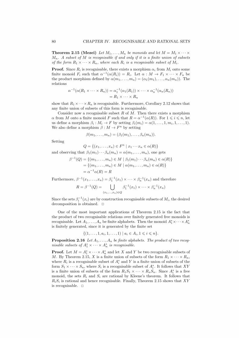
80 CHAPTER IV. RECOGNISABLE AND RATIONAL SETS
Theorem 2.15 (Mezei) Let M1, . . . ,Mn be monoids and let M =M1 × · · · ×Mn. A subset of M is recognisable if and only if it is a finite union of subsetsof the form R1 × · · · ×Rn, where each Ri is a recognisable subset of Mi.
Proof. Since Ri is recognisable, there exists a morphism αi fromMi onto somefinite monoid Fi such that α−1(α(Ri)) = Ri. Let α : M → F1 × · · · × Fn bethe product morphism defined by α(m1, . . . ,mn) = (α1(m1), . . . , αn(mn)). Therelations
α−1(α(R1 × · · · ×Rn)) = α−11 (α1(R1))× · · · × α
−1n (αn(Rn))
= R1 × · · · ×Rn
show that R1×· · ·×Rn is recognisable. Furthermore, Corollary 2.12 shows thatany finite union of subsets of this form is recognisable.
Consider now a recognisable subset R of M . Then there exists a morphismα from M onto a finite monoid F such that R = α−1(α(R)). For 1 6 i 6 n, letus define a morphism βi :Mi → F by setting βi(mi) = α(1, . . . , 1,mi, 1, . . . , 1).We also define a morphism β :M → Fn by setting
β(m1, . . . ,mn) = (β1(m1), . . . , βn(mn)).
SettingQ = {(x1, . . . , xn) ∈ F
n | x1 · · ·xn ∈ α(R)}
and observing that β1(m1) · · · βn(mn) = α(m1, . . . ,mn), one gets
β−1(Q) = {(m1, . . . ,mn) ∈M | β1(m1) · · · βn(mn) ∈ α(R)}
= {(m1, . . . ,mn) ∈M | α(m1, . . . ,mn) ∈ α(R)}
= α−1α(R) = R
Furthermore, β−1(x1, . . . , xn) = β−11 (x1)× · · · × β
−1n (xn) and therefore
R = β−1(Q) =⋃
(x1,...,xn)∈Q
β−11 (x1)× · · · × β
−1n (xn)
Since the sets β−1i (xi) are by construction recognisable subsets ofMi, the desired
decomposition is obtained.
One of the most important applications of Theorem 2.15 is the fact thatthe product of two recognisable relations over finitely generated free monoids isrecognisable. Let A1, . . . , An be finite alphabets. Then the monoid A∗
1×· · ·×A∗n
is finitely generated, since it is generated by the finite set
{(1, . . . , 1, ai, 1, . . . , 1) | ai ∈ Ai, 1 6 i 6 n}.
Proposition 2.16 Let A1, . . . , An be finite alphabets. The product of two recog-nisable subsets of A∗
1 × · · · ×A∗n is recognisable.
Proof. Let M = A∗1× · · ·×A
∗n and let X and Y be two recognisable subsets of
M . By Theorem 2.15, X is a finite union of subsets of the form R1 × · · · ×Rn,where Ri is a recognisable subset of A∗
i and Y is a finite union of subsets of theform S1 × · · · × Sn, where Si is a recognisable subset of A∗
i . It follows that XYis a finite union of subsets of the form R1S1 × · · · × RnSn. Since A∗
i is a freemonoid, the sets Ri and Si are rational by Kleene’s theorem. It follows thatRiSi is rational and hence recognisable. Finally, Theorem 2.15 shows that XYis recognisable.

3. CONNEXION WITH AUTOMATA 81
3 Connexion with automata
The case of the free monoid is of course the most important. There is a naturalway to associate a finite monoid with a finite automaton. We start by explainingthis construction for deterministic automata, which is a bit easier than thegeneral case.
3.1 Transition monoid of a deterministic automaton
Let A = (Q,A,E, q−, F ) be a deterministic automaton. Each letter a ∈ Adefines a partial transformation q → q · a on Q, which maps each state q ontothe unique state q · a (when it exists) such that (q, a, q · a) ∈ E. If there is nosuch state, q · a is undefined.
More generally, each word u defines a partial transformation q → q ·u on Q,which maps each state q onto the end state of the unique path with label u andorigin q (when it exists). One can also define q ·u by induction on the lengthof u. First, the empty word defines the identity transformation: for each stateq, q · 1 = q. Next, for every word u ∈ A+ and for every letter a ∈ A, one setsq · (ua) = (q ·u)· a if (q ·u) and (q ·u)· a are defined.
Example 3.1 Let A be the automaton of Figure III.3.4. One has 1· ba = 2,2· ba = 1 and 3· ba = 5 and for q = 4, 5, the value of q · ba is undefined. Similarly,the partial transformation associated to babbb is defined on its domain {1, 2} by1· babbb = 2 and 2· babbb = 1.
The partial function (q, a)→ q · a from Q×A into Q is called the transitionfunction of A. If A is complete, it is a total function. Note that the set Eof transitions completely determines the transition function and can also berecovered from it. For this reason, a deterministic automaton is often given asa triple (Q,A, · , q−, F ), where “·” denotes the transition function.
It follows from the definitions that the function which maps a word u ontothe partial transformation q → q ·u defines a morphism from A∗ into the monoidF(Q) of partial transformations on Q. The range of this map is a monoid, calledthe transition monoid of A.
We now present an algorithm to compute a presentation of the transitionmonoid of a finite automaton. Rather than giving a formal description of thealgorithm, we shall explain it step by step on an example. Consider the finitedeterministic automaton represented in Figure 3.1.
1 2 3
b a, c b, c
a
b
a
Figure 3.1. A deterministic automaton.
We start our computation by giving the generators of its transition monoid.

82 CHAPTER IV. RECOGNISABLE AND RATIONAL SETS
1 2 3
a 2 2 2
b 1 3 3c - 2 3
Thus a maps all states onto state 2 and c defines a partial identity: it mapsstates 2 and 3 onto themselves and is undefined on state 1.
The transition monoid is equal to the transformation monoid generated bythese generators. In order to compute it, we proceed as follows. We first fix atotal order on the alphabet, for instance a < b < c, but any total order woulddo. We also let < denote the shortlex order induced by this total order (seeSection III.1.2 for the definition). We maintain simultaneously a list of elements,in increasing order for <, and a list of rewriting rules of the form u→ v, wherev < u.
We compute the elements of the transition monoid by induction on the rankof the words in the shortlex order. The partial transformation associated withthe empty word 1 is the identity. To remember this, we add a 1 in the firstcolumn of the first row.
1 1 2 3
The partial transformations associated with the letters are the three generatorsand thus we get the following table for the words of length 6 1:
1 1 2 3
a 2 2 2
b 1 3 3c - 2 3
The general principle is now the following. Each time we consider a new wordw, we first try to use an existing rewriting rule to reduce w. If this is possible,we simply consider the next word in the shortlex order. If this is not possible,we compute the partial transformation associated with w and check whether ornot this partial transformation already appeared in our list of partial transfor-mations. If it already appeared as u, we add w → u to the list of the rewritingrules, otherwise, we add w to the list of elements. Let us also mention a conve-nient trick to compute the partial transformation associated with w when w isirreducible. Suppose that w = px, where x is a letter. Since w is irreducible, sois p and hence p is certainly in the list of elements. Therefore we already knowthe partial transformation associated with p and it suffices to compose it withx to get the partial transformation associated with w.
Let us go back to our example. Since we already considered the words oflength 6 1, we now consider the first word of length 2, namely aa. The partialtransformation associated with aa can be computed directly by following thetransition on Figure 3.1, or by using the table below. One can see that aadefines the same partial transformation as a and thus we add the rewriting ruleaa → a to our list. Next, we compute ab. This transformation maps all statesto 3 and is a new partial transformation. We then proceed by computing ac,which defines the same partial transformation as a, and then, ba, bb (which givethe new rewriting rules ba→ a and bb→ b), bc and ca (which define new partialtransformations) and cb and cc (which give the new rewriting rules cb→ bc andcc→ c). At this stage our two lists look like this:
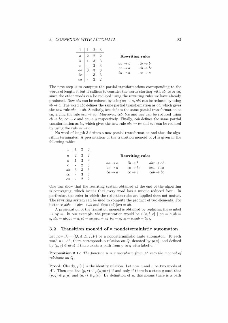
3. CONNEXION WITH AUTOMATA 83
1 1 2 3
a 2 2 2
b 1 3 3c - 2 3ab 3 3 3bc - 3 3ca - 2 2
Rewriting rules
aa→ a bb→ bac→ a cb→ bcba→ a cc→ c
The next step is to compute the partial transformations corresponding to thewords of length 3, but it suffices to consider the words starting with ab, bc or ca,since the other words can be reduced using the rewriting rules we have alreadyproduced. Now aba can be reduced by using ba→ a, abb can be reduced by usingbb→ b. The word abc defines the same partial transformation as ab, which givesthe new rule abc→ ab. Similarly, bca defines the same partial transformation asca, giving the rule bca → ca. Moreover, bcb, bcc and caa can be reduced usingcb → bc, cc → c and aa → a respectively. Finally, cab defines the same partialtransformation as bc, which gives the new rule abc→ bc and cac can be reducedby using the rule ac→ a.
No word of length 3 defines a new partial transformation and thus the algo-rithm terminates. A presentation of the transition monoid of A is given in thefollowing table:
1 1 2 3
a 2 2 2
b 1 3 3c - 2 3ab 3 3 3bc - 3 3ca - 2 2
Rewriting rules
aa→ a bb→ b abc→ abac→ a cb→ bc bca→ caba→ a cc→ c cab→ bc
One can show that the rewriting system obtained at the end of the algorithmis converging, which means that every word has a unique reduced form. Inparticular, the order in which the reduction rules are applied does not matter.The rewriting system can be used to compute the product of two elements. Forinstance abbc→ abc→ ab and thus (ab)(bc) = ab.
A presentation of the transition monoid is obtained by replacing the symbol→ by =. In our example, the presentation would be 〈 {a, b, c} | aa = a, bb =b, abc = ab, ac = a, cb = bc, bca = ca, ba = a, cc = c, cab = bc 〉.
3.2 Transition monoid of a nondeterministic automaton
Let now A = (Q,A,E, I, F ) be a nondeterministic finite automaton. To eachword u ∈ A∗, there corresponds a relation on Q, denoted by µ(u), and definedby (p, q) ∈ µ(u) if there exists a path from p to q with label u.
Proposition 3.17 The function µ is a morphism from A∗ into the monoid ofrelations on Q.
Proof. Clearly, µ(1) is the identity relation. Let now u and v be two words ofA∗. Then one has (p, r) ∈ µ(u)µ(v) if and only if there is a state q such that(p, q) ∈ µ(u) and (q, r) ∈ µ(v). By definition of µ, this means there is a path
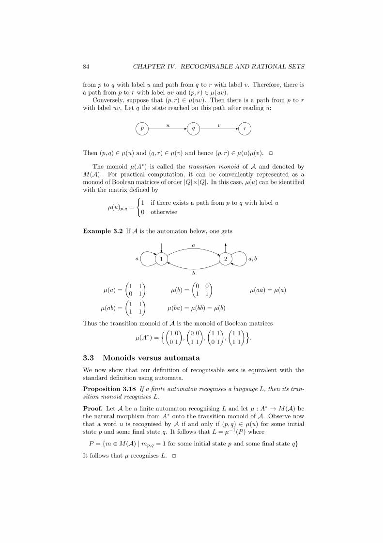
84 CHAPTER IV. RECOGNISABLE AND RATIONAL SETS
from p to q with label u and path from q to r with label v. Therefore, there isa path from p to r with label uv and (p, r) ∈ µ(uv).
Conversely, suppose that (p, r) ∈ µ(uv). Then there is a path from p to rwith label uv. Let q the state reached on this path after reading u:
p q ru v
Then (p, q) ∈ µ(u) and (q, r) ∈ µ(v) and hence (p, r) ∈ µ(u)µ(v).
The monoid µ(A∗) is called the transition monoid of A and denoted byM(A). For practical computation, it can be conveniently represented as amonoid of Boolean matrices of order |Q|×|Q|. In this case, µ(u) can be identifiedwith the matrix defined by
µ(u)p,q =
{1 if there exists a path from p to q with label u
0 otherwise
Example 3.2 If A is the automaton below, one gets
1a 2 a, b
a
b
µ(a) =
(1 10 1
)µ(b) =
(0 01 1
)µ(aa) = µ(a)
µ(ab) =
(1 11 1
)µ(ba) = µ(bb) = µ(b)
Thus the transition monoid of A is the monoid of Boolean matrices
µ(A∗) ={(1 0
0 1
),
(0 0
1 1
),
(1 1
0 1
),
(1 1
1 1
)}.
3.3 Monoids versus automata
We now show that our definition of recognisable sets is equivalent with thestandard definition using automata.
Proposition 3.18 If a finite automaton recognises a language L, then its tran-sition monoid recognises L.
Proof. Let A be a finite automaton recognising L and let µ : A∗ → M(A) bethe natural morphism from A∗ onto the transition monoid of A. Observe nowthat a word u is recognised by A if and only if (p, q) ∈ µ(u) for some initialstate p and some final state q. It follows that L = µ−1(P ) where
P = {m ∈M(A) | mp,q = 1 for some initial state p and some final state q}
It follows that µ recognises L.
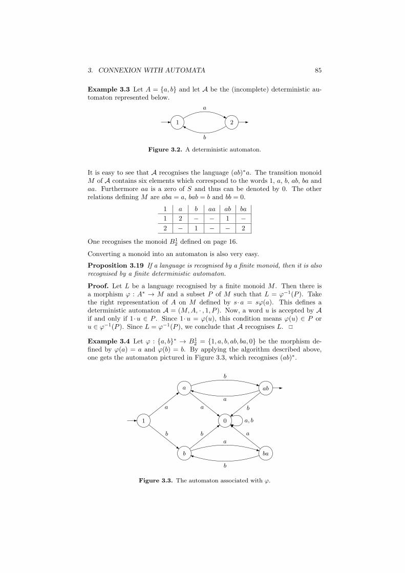
3. CONNEXION WITH AUTOMATA 85
Example 3.3 Let A = {a, b} and let A be the (incomplete) deterministic au-tomaton represented below.
1 2
a
b
Figure 3.2. A deterministic automaton.
It is easy to see that A recognises the language (ab)∗a. The transition monoidM of A contains six elements which correspond to the words 1, a, b, ab, ba andaa. Furthermore aa is a zero of S and thus can be denoted by 0. The otherrelations defining M are aba = a, bab = b and bb = 0.
1 a b aa ab ba
1 2 − − 1 −
2 − 1 − − 2
One recognises the monoid B12 defined on page 16.
Converting a monoid into an automaton is also very easy.
Proposition 3.19 If a language is recognised by a finite monoid, then it is alsorecognised by a finite deterministic automaton.
Proof. Let L be a language recognised by a finite monoid M . Then there isa morphism ϕ : A∗ → M and a subset P of M such that L = ϕ−1(P ). Takethe right representation of A on M defined by s· a = sϕ(a). This defines adeterministic automaton A = (M,A, · , 1, P ). Now, a word u is accepted by Aif and only if 1·u ∈ P . Since 1·u = ϕ(u), this condition means ϕ(u) ∈ P oru ∈ ϕ−1(P ). Since L = ϕ−1(P ), we conclude that A recognises L.
Example 3.4 Let ϕ : {a, b}∗ → B12 = {1, a, b, ab, ba, 0} be the morphism de-
fined by ϕ(a) = a and ϕ(b) = b. By applying the algorithm described above,one gets the automaton pictured in Figure 3.3, which recognises (ab)∗.
a ab
1 0
b ba
a a b
b b a
b
a
a, b
a
b
Figure 3.3. The automaton associated with ϕ.

86 CHAPTER IV. RECOGNISABLE AND RATIONAL SETS
We can now summarise the results of this section.
Theorem 3.20 Let L be a language. The following conditions are equivalent
(1) L is recognised by a finite deterministic automaton,
(2) L is recognised by a finite automaton,
(3) L is recognised by a finite monoid.
Proof. (1) implies (2) is clear and (2) implies (3) follows from Proposition 3.18.Finally, (3) implies (1) follows from Proposition 3.19.
This result implies that any finite automaton is equivalent to a deterministicone, a good illustration of the power of the algebraic approach. Indeed, theusual proof requires the subset construction, but the proof is straightforwardwith monoids.
4 The syntactic monoid
The syntactic congruence is one of the key notions of this chapter. Roughlyspeaking, it is the monoid analog of the notion of a minimal automaton, but itcan be defined for any subset of a monoid.
4.1 Definitions
The main definition was already given in Section II.3.7. Given a subset L of Mthe syntactic congruence of L in M is the relation ∼L defined on M by u ∼L vif and only if, for all x, y ∈M ,
xuy ∈ L⇐⇒ xvy ∈ L (4.1)
The quotient M/∼L is the syntactic monoid of L and the natural morphismηL : M → M/∼L is the syntactic morphism of L. Finally, the set ηL(L) iscalled the syntactic image of L. The syntactic monoid of a language L is oftendenoted by M(L) and we shall freely use this notation.
The syntactic congruence is characterised by the following property.
Proposition 4.21 The syntactic congruence of L is the coarsest congruencethat saturates L. Furthermore, a congruence ∼ saturates L if and only if ∼L iscoarser than ∼.
Proof. We first need to show that ∼L saturates L. Suppose that u ∈ L andu ∼L v. Then, one has, by taking x = y = 1 in (4.1),
u ∈ L⇐⇒ v ∈ L
and thus v ∈ L. It follows that ηL recognises L.Suppose now that a congruence ∼ saturates L and that u ∼ v. Since ∼ is a
congruence, we also have xuy ∼ xvy for every x, y ∈ M . Since ∼ saturates L,it follows that xuy ∈ L if and only if xvy ∈ L and hence u ∼L v. Therefore, ∼L
is coarser than ∼.Finally, if ∼L is coarser than ∼, the condition u ∼ v implies u ∼L v. There-
fore, if u ∈ L, then v ∈ L and ∼ saturates L.
It is sometimes convenient to state this result in terms of morphisms:
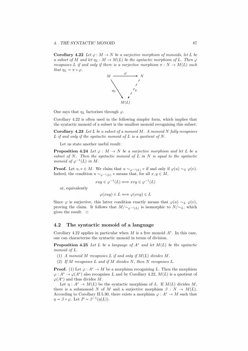
4. THE SYNTACTIC MONOID 87
Corollary 4.22 Let ϕ :M → N be a surjective morphism of monoids, let L bea subset of M and let ηL :M →M(L) be the syntactic morphism of L. Then ϕrecognises L if and only if there is a surjective morphism π : N → M(L) suchthat ηL = π ◦ ϕ.
M(L)
M N
ηL π
ϕ
One says that ηL factorises through ϕ.
Corollary 4.22 is often used in the following simpler form, which implies thatthe syntactic monoid of a subset is the smallest monoid recognising this subset.
Corollary 4.23 Let L be a subset of a monoidM . A monoid N fully recognisesL if and only if the syntactic monoid of L is a quotient of N .
Let us state another useful result:
Proposition 4.24 Let ϕ : M → N be a surjective morphism and let L be asubset of N . Then the syntactic monoid of L in N is equal to the syntacticmonoid of ϕ−1(L) in M .
Proof. Let u, v ∈ M . We claim that u ∼ϕ−1(L) v if and only if ϕ(u) ∼L ϕ(v).Indeed, the condition u ∼ϕ−1(L) v means that, for all x, y ∈M ,
xuy ∈ ϕ−1(L)⇐⇒ xvy ∈ ϕ−1(L)
or, equivalently
ϕ(xuy) ∈ L⇐⇒ ϕ(xvy) ∈ L
Since ϕ is surjective, this latter condition exactly means that ϕ(u) ∼L ϕ(v),proving the claim. It follows that M/∼ϕ−1(L) is isomorphic to N/∼L, whichgives the result.
4.2 The syntactic monoid of a language
Corollary 4.22 applies in particular when M is a free monoid A∗. In this case,one can characterise the syntactic monoid in terms of division.
Proposition 4.25 Let L be a language of A∗ and let M(L) be the syntacticmonoid of L.
(1) A monoid M recognises L if and only if M(L) divides M .
(2) If M recognises L and if M divides N , then N recognises L.
Proof. (1) Let ϕ : A∗ →M be a morphism recognising L. Then the morphismϕ : A∗ → ϕ(A∗) also recognises L and by Corollary 4.22, M(L) is a quotient ofϕ(A∗) and thus divides M .
Let η : A∗ → M(L) be the syntactic morphism of L. If M(L) divides M ,there is a submonoid N of M and a surjective morphism β : N → M(L).According to Corollary II.5.30, there exists a morphism ϕ : A∗ →M such thatη = β ◦ ϕ. Let P = β−1(η(L)).
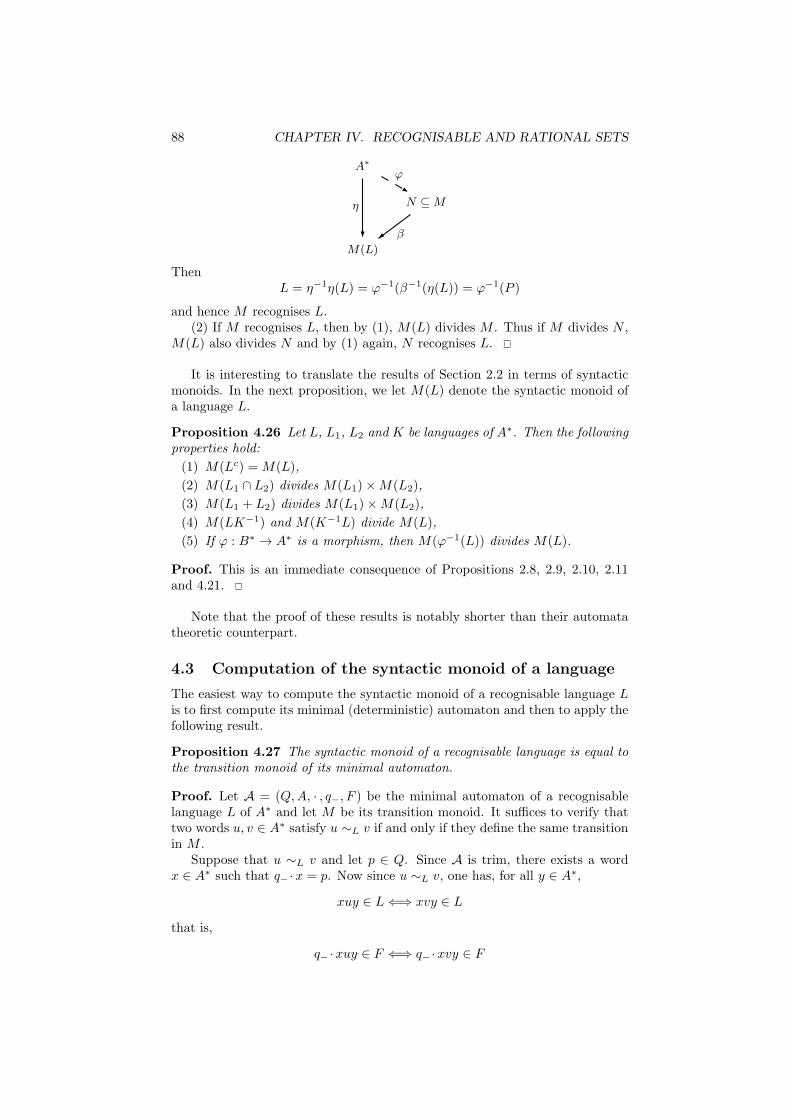
88 CHAPTER IV. RECOGNISABLE AND RATIONAL SETS
A∗
M(L)
N ⊆ Mη
ϕ
β
ThenL = η−1η(L) = ϕ−1(β−1(η(L)) = ϕ−1(P )
and hence M recognises L.(2) If M recognises L, then by (1), M(L) divides M . Thus if M divides N ,
M(L) also divides N and by (1) again, N recognises L.
It is interesting to translate the results of Section 2.2 in terms of syntacticmonoids. In the next proposition, we let M(L) denote the syntactic monoid ofa language L.
Proposition 4.26 Let L, L1, L2 and K be languages of A∗. Then the followingproperties hold:
(1) M(Lc) =M(L),
(2) M(L1 ∩ L2) divides M(L1)×M(L2),
(3) M(L1 + L2) divides M(L1)×M(L2),
(4) M(LK−1) and M(K−1L) divide M(L),
(5) If ϕ : B∗ → A∗ is a morphism, then M(ϕ−1(L)) divides M(L).
Proof. This is an immediate consequence of Propositions 2.8, 2.9, 2.10, 2.11and 4.21.
Note that the proof of these results is notably shorter than their automatatheoretic counterpart.
4.3 Computation of the syntactic monoid of a language
The easiest way to compute the syntactic monoid of a recognisable language Lis to first compute its minimal (deterministic) automaton and then to apply thefollowing result.
Proposition 4.27 The syntactic monoid of a recognisable language is equal tothe transition monoid of its minimal automaton.
Proof. Let A = (Q,A, · , q−, F ) be the minimal automaton of a recognisablelanguage L of A∗ and let M be its transition monoid. It suffices to verify thattwo words u, v ∈ A∗ satisfy u ∼L v if and only if they define the same transitionin M .
Suppose that u ∼L v and let p ∈ Q. Since A is trim, there exists a wordx ∈ A∗ such that q− ·x = p. Now since u ∼L v, one has, for all y ∈ A∗,
xuy ∈ L⇐⇒ xvy ∈ L
that is,
q− ·xuy ∈ F ⇐⇒ q− ·xvy ∈ F
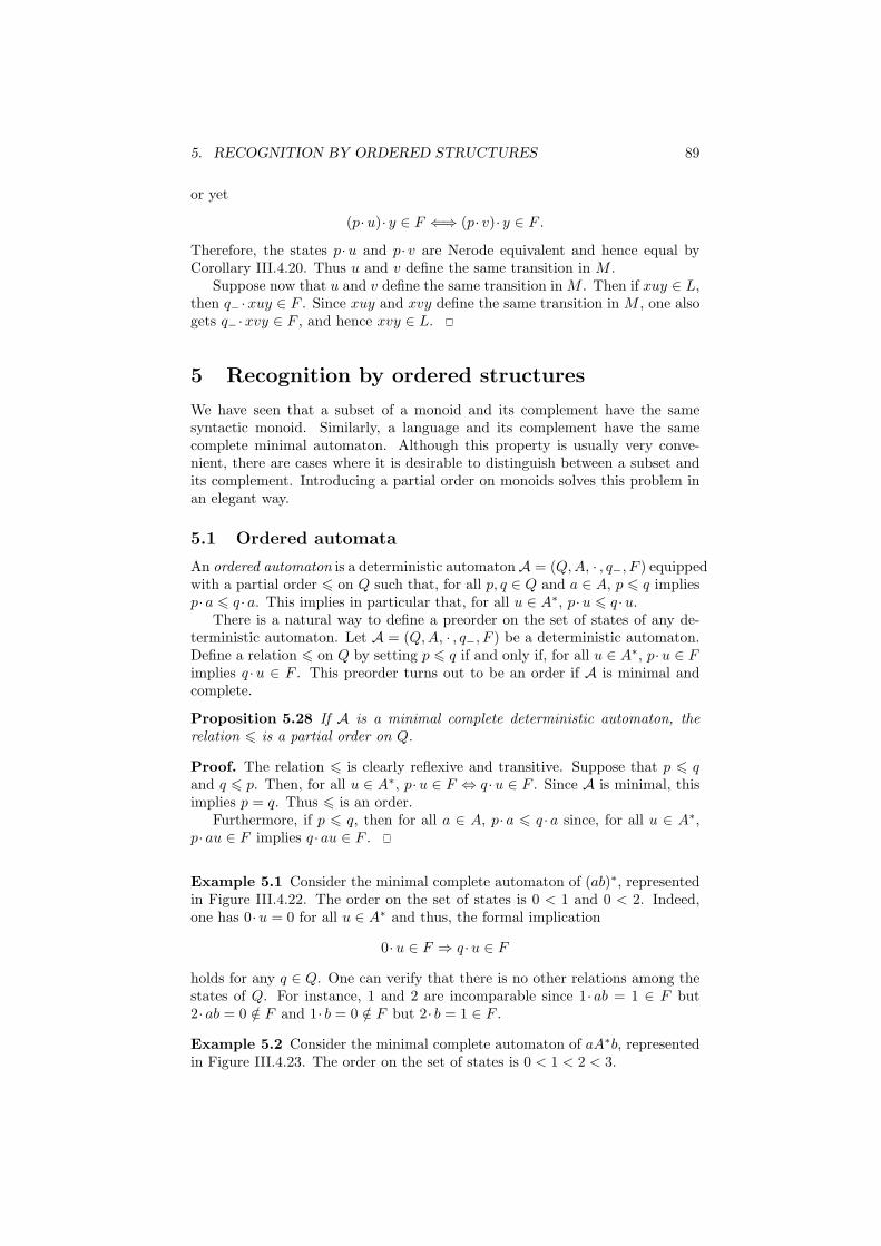
5. RECOGNITION BY ORDERED STRUCTURES 89
or yet
(p·u)· y ∈ F ⇐⇒ (p· v)· y ∈ F .
Therefore, the states p·u and p· v are Nerode equivalent and hence equal byCorollary III.4.20. Thus u and v define the same transition in M .
Suppose now that u and v define the same transition inM . Then if xuy ∈ L,then q− ·xuy ∈ F . Since xuy and xvy define the same transition in M , one alsogets q− ·xvy ∈ F , and hence xvy ∈ L.
5 Recognition by ordered structures
We have seen that a subset of a monoid and its complement have the samesyntactic monoid. Similarly, a language and its complement have the samecomplete minimal automaton. Although this property is usually very conve-nient, there are cases where it is desirable to distinguish between a subset andits complement. Introducing a partial order on monoids solves this problem inan elegant way.
5.1 Ordered automata
An ordered automaton is a deterministic automatonA = (Q,A, · , q−, F ) equippedwith a partial order 6 on Q such that, for all p, q ∈ Q and a ∈ A, p 6 q impliesp· a 6 q · a. This implies in particular that, for all u ∈ A∗, p·u 6 q ·u.
There is a natural way to define a preorder on the set of states of any de-terministic automaton. Let A = (Q,A, · , q−, F ) be a deterministic automaton.Define a relation 6 on Q by setting p 6 q if and only if, for all u ∈ A∗, p·u ∈ Fimplies q ·u ∈ F . This preorder turns out to be an order if A is minimal andcomplete.
Proposition 5.28 If A is a minimal complete deterministic automaton, therelation 6 is a partial order on Q.
Proof. The relation 6 is clearly reflexive and transitive. Suppose that p 6 qand q 6 p. Then, for all u ∈ A∗, p·u ∈ F ⇔ q ·u ∈ F . Since A is minimal, thisimplies p = q. Thus 6 is an order.
Furthermore, if p 6 q, then for all a ∈ A, p· a 6 q · a since, for all u ∈ A∗,p· au ∈ F implies q · au ∈ F .
Example 5.1 Consider the minimal complete automaton of (ab)∗, representedin Figure III.4.22. The order on the set of states is 0 < 1 and 0 < 2. Indeed,one has 0·u = 0 for all u ∈ A∗ and thus, the formal implication
0·u ∈ F ⇒ q ·u ∈ F
holds for any q ∈ Q. One can verify that there is no other relations among thestates of Q. For instance, 1 and 2 are incomparable since 1· ab = 1 ∈ F but2· ab = 0 /∈ F and 1· b = 0 /∈ F but 2· b = 1 ∈ F .
Example 5.2 Consider the minimal complete automaton of aA∗b, representedin Figure III.4.23. The order on the set of states is 0 < 1 < 2 < 3.

90 CHAPTER IV. RECOGNISABLE AND RATIONAL SETS
5.2 Recognition by ordered monoids
A congruence on an ordered monoid (M,6) is a stable preorder which is coarserthan 6. In particular, the order relation 6 is itself a congruence. If 4 is acongruence on (M,6), then the equivalence relation ∼ associated with 4 isa congruence on M . Furthermore, there is a well-defined stable order on thequotient set M/∼, given by
[s] 6 [t] if and only if s 4 t
Thus (M/∼,6) is an ordered monoid, also denoted by M/4.Let ϕ : M → N be a surjective morphism of ordered monoids. A subset Q
of M is recognised by ϕ if there exists an upper set P of N such that
Q = ϕ−1(P )
This condition implies that Q is an upper set of M and that
ϕ(Q) = ϕ(ϕ−1(P )) = P
By extension, a subset Q of M is said to be recognised by an ordered monoid Nif there exists a surjective morphism of ordered monoids from M onto N thatrecognises Q.
It is sometimes convenient to formulate this definition in terms of congru-ences. Let M be an ordered monoid and let 4 a congruence on M . A subset Qof M is said to be recognised by 4 if, for every q ∈ Q, q 4 p implies p ∈ Q. Itis easy to see that a surjective morphism of ordered monoids ϕ recognises Q ifand only if the nuclear congruence 4ϕ recognises Q.
How does this definition relate to the standard definition using monoids?Simply by considering a monoid as an ordered monoid, with the equality relationas an order relation.
Example 5.3 Consider the monoidB12 = {1, a, b, ab, ba, 0} and let π : {a, b}∗ →
M be the morphism defined by π(a) = a and π(b) = b. Let us define an order onB1
2 by setting ab 6 1, ba 6 1, and 0 6 x for all x ∈ B12 . Then the set I = {1, ab}
is an upper set and π−1(I) = (ab)∗. Thus the language (ab)∗ is recognised bythe ordered monoid (B1
2 ,6).
It suffices to reverse the order to recognise the complement of a language.
Proposition 5.29 Let L be a language of A∗. If L is recognised by an orderedmonoid (M,6), then Lc is recognised by the ordered monoid (M,>).
Proof. Let ϕ : A∗ → M be a morphism and let P be an upper set of (M,6)such that ϕ−1(P ) = L. Then ϕ−1(P c) = Lc and it suffices to show that P c isa >-upper set. Suppose that x ∈ P c and x > y. If y ∈ P , then x ∈ P , since Pis a 6-upper set. Thus y ∈ P c, which concludes the proof.
5.3 Syntactic order
First note that, if (M,6) is an ordered monoid, the congruence 6 recognisesevery upper set of M . The syntactic congruence of an upper set Q of M is thecoarsest congruence among the congruences on M that recognise Q.
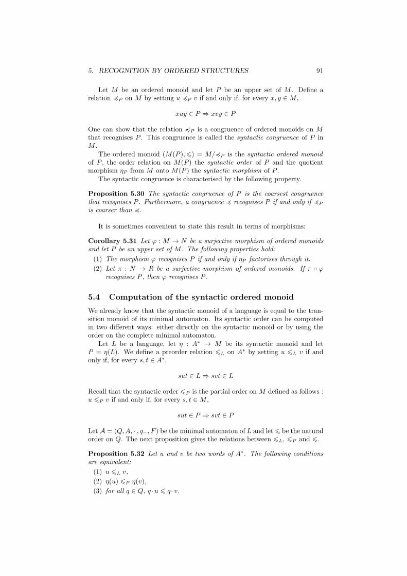
5. RECOGNITION BY ORDERED STRUCTURES 91
Let M be an ordered monoid and let P be an upper set of M . Define arelation 4P on M by setting u 4P v if and only if, for every x, y ∈M ,
xuy ∈ P ⇒ xvy ∈ P
One can show that the relation 4P is a congruence of ordered monoids on Mthat recognises P . This congruence is called the syntactic congruence of P inM .
The ordered monoid (M(P ),6) = M/4P is the syntactic ordered monoidof P , the order relation on M(P ) the syntactic order of P and the quotientmorphism ηP from M onto M(P ) the syntactic morphism of P .
The syntactic congruence is characterised by the following property.
Proposition 5.30 The syntactic congruence of P is the coarsest congruencethat recognises P . Furthermore, a congruence 4 recognises P if and only if 4P
is coarser than 4.
It is sometimes convenient to state this result in terms of morphisms:
Corollary 5.31 Let ϕ : M → N be a surjective morphism of ordered monoidsand let P be an upper set of M . The following properties hold:
(1) The morphism ϕ recognises P if and only if ηP factorises through it.
(2) Let π : N → R be a surjective morphism of ordered monoids. If π ◦ ϕrecognises P , then ϕ recognises P .
5.4 Computation of the syntactic ordered monoid
We already know that the syntactic monoid of a language is equal to the tran-sition monoid of its minimal automaton. Its syntactic order can be computedin two different ways: either directly on the syntactic monoid or by using theorder on the complete minimal automaton.
Let L be a language, let η : A∗ → M be its syntactic monoid and letP = η(L). We define a preorder relation 6L on A∗ by setting u 6L v if andonly if, for every s, t ∈ A∗,
sut ∈ L⇒ svt ∈ L
Recall that the syntactic order 6P is the partial order on M defined as follows :u 6P v if and only if, for every s, t ∈M ,
sut ∈ P ⇒ svt ∈ P
Let A = (Q,A, · , q−, F ) be the minimal automaton of L and let 6 be the naturalorder on Q. The next proposition gives the relations between 6L, 6P and 6.
Proposition 5.32 Let u and v be two words of A∗. The following conditionsare equivalent:
(1) u 6L v,
(2) η(u) 6P η(v),
(3) for all q ∈ Q, q ·u 6 q · v.
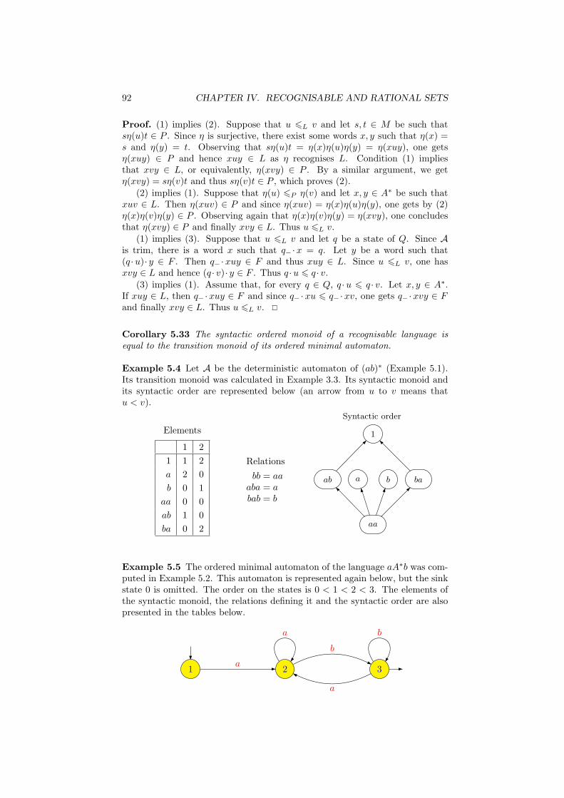
92 CHAPTER IV. RECOGNISABLE AND RATIONAL SETS
Proof. (1) implies (2). Suppose that u 6L v and let s, t ∈ M be such thatsη(u)t ∈ P . Since η is surjective, there exist some words x, y such that η(x) =s and η(y) = t. Observing that sη(u)t = η(x)η(u)η(y) = η(xuy), one getsη(xuy) ∈ P and hence xuy ∈ L as η recognises L. Condition (1) impliesthat xvy ∈ L, or equivalently, η(xvy) ∈ P . By a similar argument, we getη(xvy) = sη(v)t and thus sη(v)t ∈ P , which proves (2).
(2) implies (1). Suppose that η(u) 6P η(v) and let x, y ∈ A∗ be such thatxuv ∈ L. Then η(xuv) ∈ P and since η(xuv) = η(x)η(u)η(y), one gets by (2)η(x)η(v)η(y) ∈ P . Observing again that η(x)η(v)η(y) = η(xvy), one concludesthat η(xvy) ∈ P and finally xvy ∈ L. Thus u 6L v.
(1) implies (3). Suppose that u 6L v and let q be a state of Q. Since Ais trim, there is a word x such that q− ·x = q. Let y be a word such that(q ·u)· y ∈ F . Then q− ·xuy ∈ F and thus xuy ∈ L. Since u 6L v, one hasxvy ∈ L and hence (q · v)· y ∈ F . Thus q ·u 6 q · v.
(3) implies (1). Assume that, for every q ∈ Q, q ·u 6 q · v. Let x, y ∈ A∗.If xuy ∈ L, then q− ·xuy ∈ F and since q− ·xu 6 q− ·xv, one gets q− ·xvy ∈ Fand finally xvy ∈ L. Thus u 6L v.
Corollary 5.33 The syntactic ordered monoid of a recognisable language isequal to the transition monoid of its ordered minimal automaton.
Example 5.4 Let A be the deterministic automaton of (ab)∗ (Example 5.1).Its transition monoid was calculated in Example 3.3. Its syntactic monoid andits syntactic order are represented below (an arrow from u to v means thatu < v).
Elements
1 2
1 1 2
a 2 0
b 0 1
aa 0 0
ab 1 0
ba 0 2
Relations
bb = aaaba = abab = b
ab a b ba
aa
1
Syntactic order
Example 5.5 The ordered minimal automaton of the language aA∗b was com-puted in Example 5.2. This automaton is represented again below, but the sinkstate 0 is omitted. The order on the states is 0 < 1 < 2 < 3. The elements ofthe syntactic monoid, the relations defining it and the syntactic order are alsopresented in the tables below.
1 2 3
a b
a
a
b
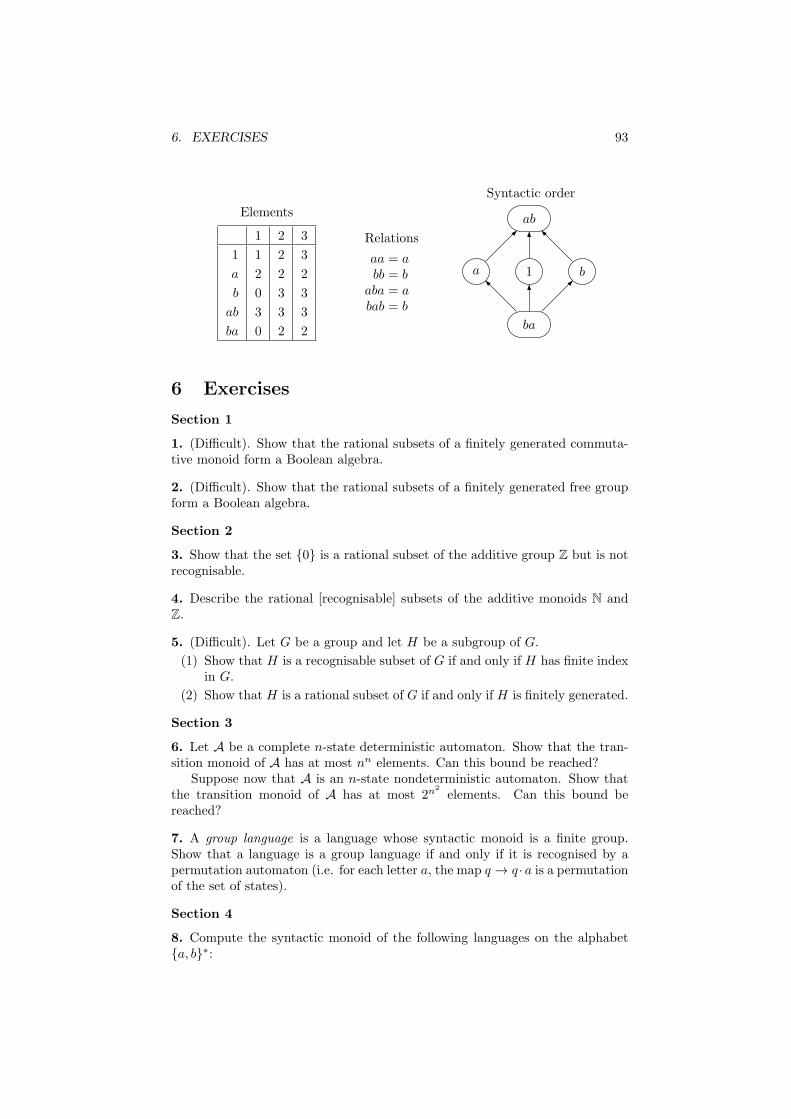
6. EXERCISES 93
Elements
1 2 3
1 1 2 3
a 2 2 2
b 0 3 3
ab 3 3 3
ba 0 2 2
Relations
aa = abb = baba = abab = b
ab
a 1 b
ba
Syntactic order
6 Exercises
Section 1
1. (Difficult). Show that the rational subsets of a finitely generated commuta-tive monoid form a Boolean algebra.
2. (Difficult). Show that the rational subsets of a finitely generated free groupform a Boolean algebra.
Section 2
3. Show that the set {0} is a rational subset of the additive group Z but is notrecognisable.
4. Describe the rational [recognisable] subsets of the additive monoids N andZ.
5. (Difficult). Let G be a group and let H be a subgroup of G.
(1) Show that H is a recognisable subset of G if and only if H has finite indexin G.
(2) Show that H is a rational subset of G if and only if H is finitely generated.
Section 3
6. Let A be a complete n-state deterministic automaton. Show that the tran-sition monoid of A has at most nn elements. Can this bound be reached?
Suppose now that A is an n-state nondeterministic automaton. Show thatthe transition monoid of A has at most 2n
2
elements. Can this bound bereached?
7. A group language is a language whose syntactic monoid is a finite group.Show that a language is a group language if and only if it is recognised by apermutation automaton (i.e. for each letter a, the map q → q · a is a permutationof the set of states).
Section 4
8. Compute the syntactic monoid of the following languages on the alphabet{a, b}∗:
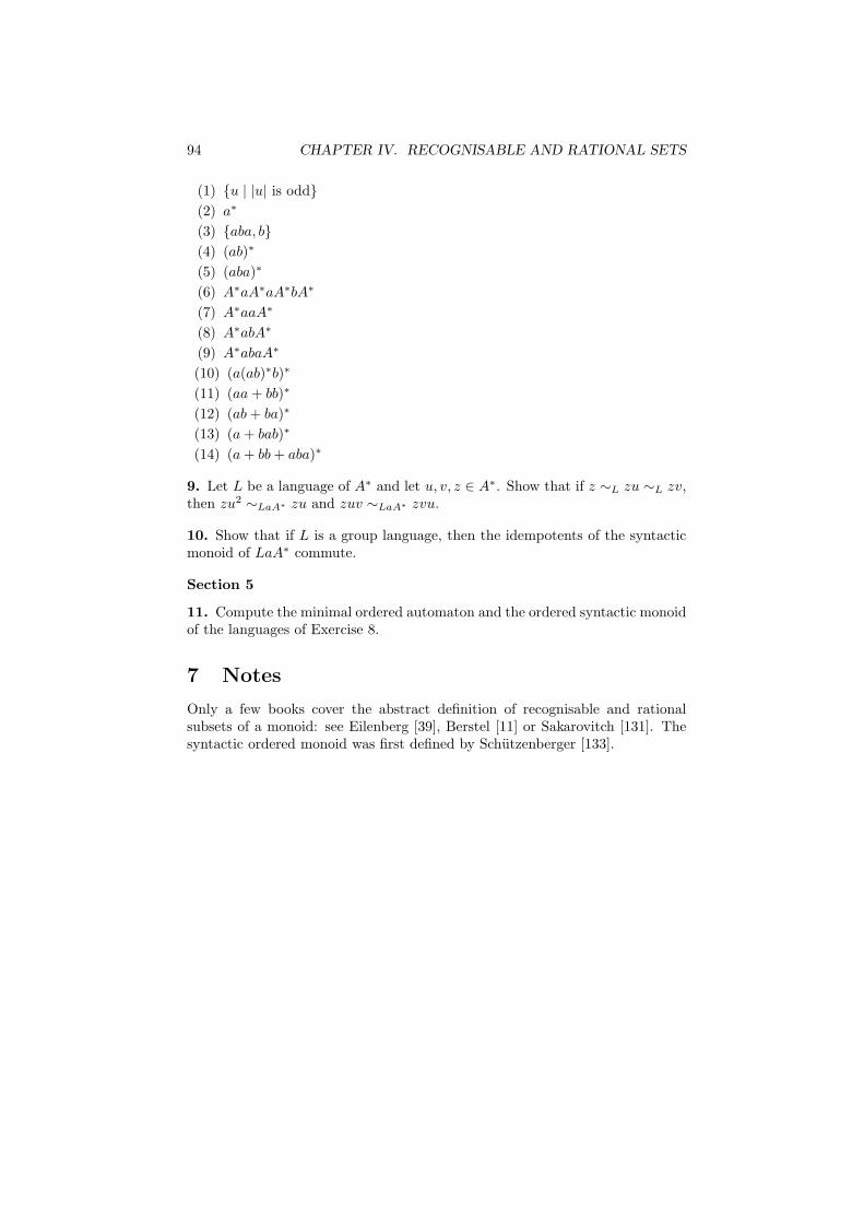
94 CHAPTER IV. RECOGNISABLE AND RATIONAL SETS
(1) {u | |u| is odd}
(2) a∗
(3) {aba, b}
(4) (ab)∗
(5) (aba)∗
(6) A∗aA∗aA∗bA∗
(7) A∗aaA∗
(8) A∗abA∗
(9) A∗abaA∗
(10) (a(ab)∗b)∗
(11) (aa+ bb)∗
(12) (ab+ ba)∗
(13) (a+ bab)∗
(14) (a+ bb+ aba)∗
9. Let L be a language of A∗ and let u, v, z ∈ A∗. Show that if z ∼L zu ∼L zv,then zu2 ∼LaA∗ zu and zuv ∼LaA∗ zvu.
10. Show that if L is a group language, then the idempotents of the syntacticmonoid of LaA∗ commute.
Section 5
11. Compute the minimal ordered automaton and the ordered syntactic monoidof the languages of Exercise 8.
7 Notes
Only a few books cover the abstract definition of recognisable and rationalsubsets of a monoid: see Eilenberg [39], Berstel [11] or Sakarovitch [131]. Thesyntactic ordered monoid was first defined by Schutzenberger [133].

Chapter V
Green’s relations and local
theory
Green’s relations were introduced and studied by Green in 1951 [52]. Theserelations can be considered as a noncommutative generalisation to semigroupsof the standard notion of being a multiple among integers or polynomials. Theyalso have a natural interpretation in the Cayley graph of an A-generated monoid.They are essential for understanding the structure of semigroups.
1 Green’s relations
Let S be a semigroup. We define on S four preorder relations 6R,6L,6J and6H as follows
s 6R t if and only if s = tu for some u ∈ S1
s 6L t if and only if s = ut for some u ∈ S1
s 6J t if and only if s = utv for some u, v ∈ S1
s 6H t if and only if s 6R t and s 6L t
These relations can be considered as a noncommutative generalisation of thenotion of multiple over the integers. For instance s 6R t if s is a right multipleof t, in the sense that one can pass from t to s by right multiplication by someelement of S1. These definitions can be reformulated in terms of ideals as follows
s 6R t⇐⇒ sS1 ⊆ tS1
s 6L t⇐⇒ S1s ⊆ S1t
s 6J t⇐⇒ S1sS1 ⊆ S1tS1
s 6H t⇐⇒ s 6R t and s 6L t
Thus s 6J t [s 6R t, s 6L t] if the ideal [right ideal, left ideal] generated bys is contained in the ideal [right ideal, left ideal] generated by t. The followingdiagram summarises the connexions between these four preorders.
95

96 CHAPTER V. GREEN’S RELATIONS AND LOCAL THEORY
s 6H t
s 6R t
s 6L t
s 6J t
The equivalences associated with these four preorder relations are denoted byR, L, J and H, respectively. Therefore
s R t⇐⇒ sS1 = tS1
s L t⇐⇒ S1s = S1t
s J t⇐⇒ S1sS1 = S1tS1
s H t⇐⇒ s R t and s L t
Thus two elements s and t are R-equivalent if they generate the same rightideal, or, equivalently, if there exist p, q ∈ S1 such that s = tp and t = sq.The equivalence classes of the relation R are the R-classes of S. The L-classes,J -classes and H-classes are defined in a similar way. If s is an element of S,its R-class [L-class, J -class, H-class] is denoted by R(s) [L(s), J(s), H(s)]. IfK is one of the Green’s relations, we shall use the notation s <K t if s 6K t buts 6K t.
If M is an A-generated monoid, the relations R and 6R [L and 6L] have anatural interpretation on the right [left] Cayley graph of M .
Proposition 1.1 Let M be an A-generated monoid and let s, t ∈ M . Thens 6R t [s 6L t] if and only if there is a path from t to s in the right [left ] Cayleygraph of M . Furthermore s R t [s L t] if and only if s and t are in the samestrongly connected component of the right [left ] Cayley graph of M .
Proof. Suppose that s 6R t. Then tp = s for some p ∈ M . Since M is A-generated, p can be written as a product of elements of A, say p = a1 · · · an.Therefore there is a path
sa1−→ sa1
a2−→ · · · s(a1 · · · an−1)an−→ s(a1 · · · an) = t
The other cases are similar.
It follows in particular that the R-classes [L-classes] of M correspond to thestrongly connected components of the right [left] Cayley graph.
Example 1.1 Let us consider the monoid M considered in Section IV.3.1.

1. GREEN’S RELATIONS 97
1
a
b
c
ab
bc
ca
a
b
c
a, c
b
ab
c
a
b
c
a
b, c
a
b, c
a, c
b
Figure 1.1. The right Cayley graph of M .
The right Cayley graph of M is represented in Figure 1.1. The strongly con-nected components of this graph are the R-classes of M : {1}, {b}, {c}, {a, ab}and {bc, ca}.
The next propositions summarise some useful properties of Green’s relations.
Proposition 1.2 In each semigroup S, the relations 6R and R are stable onthe left and the relations 6L and L are stable on the right.
Proof. Indeed, if s 6R t, then sS1 ⊆ tS1 and thus usS1 ⊆ utS1. It followsthat us 6R ut. The other cases are analogous.
Proposition 1.3 Let S be a semigroup.
(1) Let e be an idempotent of S. Then s 6R e if and only if es = s and s 6L eif and only if se = s.
(2) If s 6R sxy, then s R sx R sxy. If s 6L yxs, then s L xs L yxs.
Proof. We shall prove only the first part of each statement, since the otherpart is dual.
(1) If s 6R e, then s = eu for some u ∈ S1. It follows that es = e(eu) =(ee)u = eu = s. Conversely, if es = s, then s 6R e by definition.
(2) If s 6R sxy, then s 6R sxy 6R sx 6R s, whence s R sx R sxy.
The first part of Proposition 1.3 can be extended to the preorder 6H.
Proposition 1.4 Let S be a semigroup. Let s ∈ S and e be an idempotent ofS. Then s 6H e if and only if es = s = se.
Proof. It follows from Proposition 1.3.
The restriction of the preorder 6H to E(S) is actually an order, called thenatural order on E(S) and denoted by 6.

98 CHAPTER V. GREEN’S RELATIONS AND LOCAL THEORY
Corollary 1.5 Let S be a semigroup and let e and f be idempotents of S. Thefollowing conditions are equivalent:
(1) e 6 f ,
(2) ef = e = fe,
(3) fef = e.
Proof. The equivalence of (1) and (2) follows from Proposition 1.4 and that of(2) and (3) from the Simplification lemma.
Despite its elementary nature, the next proposition is one of the cornerstonesof semigroup theory.
Proposition 1.6 In each semigroup S, the relations 6R and 6L [R and L]commute.
Proof. Suppose that s 6R r and r 6L t. Then s = rv and r = ut for someu, v ∈ S1. It follows that s = utv 6L tv 6R t. Thus 6L ◦6R ⊆ 6R ◦6L. Theopposite inclusion holds by duality and hence 6R and 6L commute. The prooffor R and L is similar.
Here is a first consequence of Proposition 1.6.
Proposition 1.7 The relation 6J is equal to 6L ◦6R and to 6R ◦6L. It isalso the preorder generated by 6R and 6L.
Proof. It follows directly from Proposition I.2.21.
We now introduce the fifth Green’s relation D, which is the preorder gen-erated by R and L. Propositions 1.6 and I.2.21 immediately leads to an easierdefinition.
Proposition 1.8 The relation D is equal to L ◦ R and to R ◦ L.
One can therefore give the following definition of D:
s D t⇐⇒ there exists u ∈ S such that s R u and u L t
⇐⇒ there exists v ∈ S such that s L v and v R t.
The equivalence classes of D are called the D-classes of S, and the D-class ofan element s is denoted by D(s).
It is easy to see that s D t implies s J t. Indeed, if s D t, there exists u ∈ Ssuch that s R u and u L t. It follows that sS1 = uS1 and S1u = S1t, whenceS1sS1 = S1tS1. The following diagram summarises the connexions between thefive Green’s relations.
s H t
s R t
s L t
s D t s J t

1. GREEN’S RELATIONS 99
The equality D = J does not hold in arbitrary semigroups (see Example 1.2below) but it holds for finite semigroups.
Theorem 1.9 In a finite semigroup, the Green’s relations J and D are equal.Furthermore, the following properties hold:
(1) If s 6J sx (in particular if s J sx), then s R sx;
(2) If s 6J xs (in particular if s J xs), then s L xs.
(3) If s J t and s 6R t, then s R t;
(4) If s J t and s 6L t, then s L t;
(5) if s = usv for some u, v ∈ S1, then us H s H sv.
Proof. If x D y, there exist z ∈ S such that x R z and z L y. It follows thatx J z and z J y, whence x J y.
Conversely, suppose that x J y. Then there exist s, t, u, v ∈ S1 such thaty = txu and x = syv, whence x = stxuv. By multiplying on the left by st andon the right by uv, we obtain by induction the relation (st)nx(uv)n = x for alln > 0. By Proposition II.6.33, one can choose n such that both (st)n and (uv)n
are idempotent. It follows that (st)nx = (st)n(st)nx(uv)n = (st)nx(uv)n = xand similarly x = x(uv)n. Therefore tx L x and xu R x. The first relationimplies y = txu L xu and finally y D x.
(1) If s 6J sx, there exist u, v ∈ S1 such that usxv = s. By multiplyingon the left by u and on the right by xv, we obtain by induction the relationuns(xv)n = s for all n > 0. By Proposition II.6.33, one can choose n such thatun is idempotent. It follows that s = uns(xv)n = ununs(xv)n = uns, whences(xv)n = s. It follows that s R sx, since (sx)(v(xv)n−1) = s.
(2) is dual from (1).
(3) If s 6R t, there exist u ∈ S1 such that s = tu. If further s J t, thent J tu and t R tu by (1). Thus s R t.
(4) is dual from (3).
(5) If s = usv then s 6J us. It follows by (1) that s R sv and a dualargument shows that s L us. Since the relation R is stable on the left, one hasus R usv = s and dually, sv L s. Thus us H s H sv.
Example 1.2 Let S be the infinite semigroup of matrices of the form
(a 0b 1
)
where a and b are strictly positive rational numbers, equipped with the usualmultiplication of matrices. Then the four relations R, L, H and D coincide withthe equality, but S has a single J -class.
Proposition 1.8 shows that for two elements s and t, the three conditionss D t, R(s)∩L(t) 6= ∅ and L(s)∩R(t) 6= ∅ are equivalent. It is therefore possibleto represent D-classes by an “egg-box picture”, as in Figure 1.2.
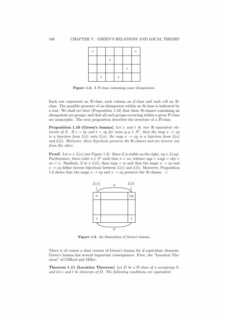
100 CHAPTER V. GREEN’S RELATIONS AND LOCAL THEORY
∗
∗
∗
∗
∗
∗
Figure 1.2. A D-class containing some idempotents.
Each row represents an R-class, each column an L-class and each cell an H-class. The possible presence of an idempotent within an H-class is indicated bya star. We shall see later (Proposition 1.13) that these H-classes containing anidempotent are groups, and that all such groups occurring within a given D-classare isomorphic. The next proposition describes the structure of a D-class.
Proposition 1.10 (Green’s lemma) Let s and t be two R-equivalent ele-ments of S. If s = tp and t = sq for some p, q ∈ S1, then the map x → xpis a bijection from L(t) onto L(s), the map x → xq is a bijection from L(s)and L(t). Moreover, these bijections preserve the H-classes and are inverse onefrom the other.
Proof. Let n ∈ L(s) (see Figure 1.3). Since L is stable on the right, nq ∈ L(sq).Furthermore, there exist u ∈ S1 such that n = us, whence nqp = usqp = utp =us = n. Similarly, if m ∈ L(t), then mpq = m and thus the maps x → xp andx→ xq define inverse bijections between L(s) and L(t). Moreover, Proposition1.2 shows that the maps x→ xp and x→ xq preserve the H-classes.
L(s)↓
L(t)↓
n nq
s t
p
q
Figure 1.3. An illustration of Green’s lemma.
There is of course a dual version of Green’s lemma for L-equivalent elements.Green’s lemma has several important consequences. First, the “Location The-orem” of Clifford and Miller:
Theorem 1.11 (Location Theorem) Let D be a D-class of a semigroup S,and let s and t be elements of D. The following conditions are equivalent:
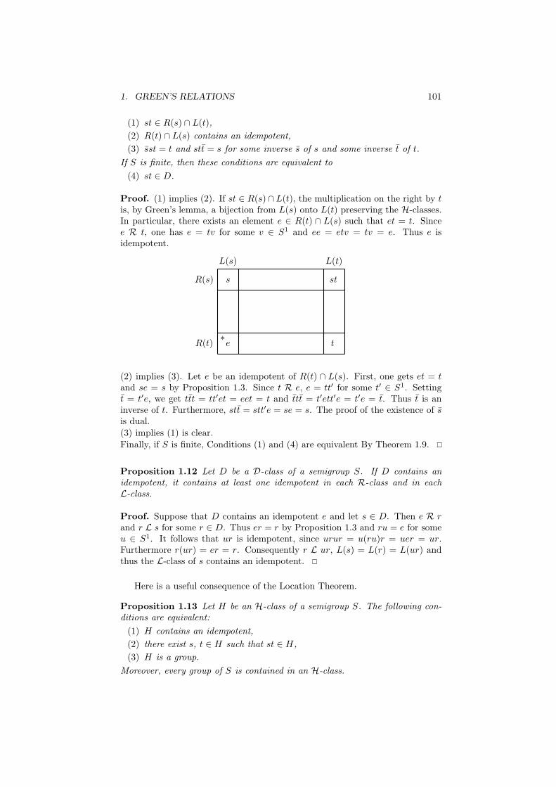
1. GREEN’S RELATIONS 101
(1) st ∈ R(s) ∩ L(t),
(2) R(t) ∩ L(s) contains an idempotent,
(3) sst = t and stt = s for some inverse s of s and some inverse t of t.
If S is finite, then these conditions are equivalent to
(4) st ∈ D.
Proof. (1) implies (2). If st ∈ R(s) ∩L(t), the multiplication on the right by tis, by Green’s lemma, a bijection from L(s) onto L(t) preserving the H-classes.In particular, there exists an element e ∈ R(t) ∩ L(s) such that et = t. Sincee R t, one has e = tv for some v ∈ S1 and ee = etv = tv = e. Thus e isidempotent.
s
t
st
e∗
L(s) L(t)
R(s)
R(t)
(2) implies (3). Let e be an idempotent of R(t) ∩ L(s). First, one gets et = tand se = s by Proposition 1.3. Since t R e, e = tt′ for some t′ ∈ S1. Settingt = t′e, we get ttt = tt′et = eet = t and ttt = t′ett′e = t′e = t. Thus t is aninverse of t. Furthermore, stt = stt′e = se = s. The proof of the existence of sis dual.
(3) implies (1) is clear.
Finally, if S is finite, Conditions (1) and (4) are equivalent By Theorem 1.9.
Proposition 1.12 Let D be a D-class of a semigroup S. If D contains anidempotent, it contains at least one idempotent in each R-class and in eachL-class.
Proof. Suppose that D contains an idempotent e and let s ∈ D. Then e R rand r L s for some r ∈ D. Thus er = r by Proposition 1.3 and ru = e for someu ∈ S1. It follows that ur is idempotent, since urur = u(ru)r = uer = ur.Furthermore r(ur) = er = r. Consequently r L ur, L(s) = L(r) = L(ur) andthus the L-class of s contains an idempotent.
Here is a useful consequence of the Location Theorem.
Proposition 1.13 Let H be an H-class of a semigroup S. The following con-ditions are equivalent:
(1) H contains an idempotent,
(2) there exist s, t ∈ H such that st ∈ H,
(3) H is a group.
Moreover, every group of S is contained in an H-class.

102 CHAPTER V. GREEN’S RELATIONS AND LOCAL THEORY
Proof. The equivalence of (1) and (2) follows from Theorem 1.11. Furthermore,it is clear that (3) implies (1). Let us show that (1) implies (3).
Let H be a H-class containing an idempotent e. Then H is a semigroup:indeed, if s, t ∈ H, we have st ∈ R(s) ∩ L(t) = H. Moreover, if s ∈ H, we haves R e and hence es = s by Proposition 1.3. Moreover, by Green’s lemma, themap x→ xs is a permutation on H. In particular, there exists t ∈ H such thatts = e, and thus H is a group with identity e.
Finally, if H is a group with identity e, then H is contained in the H-classof e. Indeed, if t is the inverse of an element s of H, then st = ts = e andse = es = s, which proves that s H e.
The following is another remarkable consequence of Green’s lemma.
Proposition 1.14 Two maximal subgroups of a D-class are isomorphic.
Proof. From Proposition 1.13, the two groups are of the form H(e) and H(f)for some idempotent e, f of the same D-class D. Since e D f , there existss ∈ R(e) ∩ L(f). Thus es = s, sf = s and ts = f for some t ∈ S1. By Green’slemma, the function ϕ defined by ϕ(x) = txs is a bijection from H(e) ontoH(f), which maps e to f since tes = ts = f .
e s
f
s
t
Figure 1.4. The D-class D.
We claim that ϕ is a morphism. First observe that st is idempotent, sincestst = sft = st. Furthermore, st R s since sts = sf = s. If y ∈ H(e), theny R e R s R st and by Proposition 1.3, (st)y = y. It follows that for allx, y ∈ H(e),
ϕ(xy) = txys = tx(sty)s = (txs)(tys) = ϕ(x)ϕ(y)
proving the claim. Thus H(e) and H(f) are isomorphic.
For finite semigroups, some further properties hold.
Corollary 1.15 Let S be a finite semigroup and let s, t ∈ S be two J -relatedelements of S. If st L s or ts R s, then H(t) is a group. If st = s or ts = s,then t is idempotent.
Proof. Suppose that st L s (the other case is dual) and let J be the commonJ -class of s, t and st. Since st 6L t, Theorem 1.9 shows that t L st, whences L t since st L s. Thus L(s) = L(t) and R(t) ∩ L(s) = H(t). Since st ∈ J ,
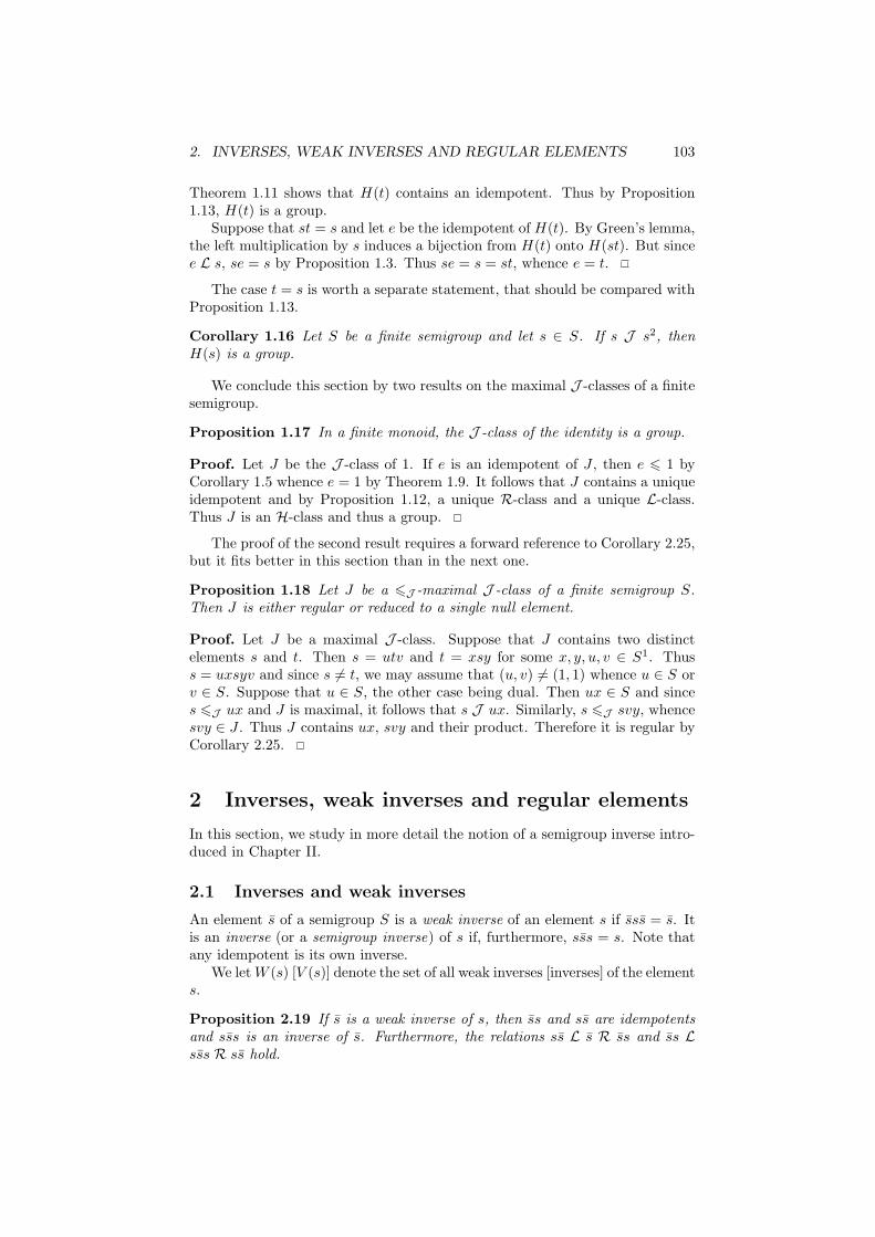
2. INVERSES, WEAK INVERSES AND REGULAR ELEMENTS 103
Theorem 1.11 shows that H(t) contains an idempotent. Thus by Proposition1.13, H(t) is a group.
Suppose that st = s and let e be the idempotent of H(t). By Green’s lemma,the left multiplication by s induces a bijection from H(t) onto H(st). But sincee L s, se = s by Proposition 1.3. Thus se = s = st, whence e = t.
The case t = s is worth a separate statement, that should be compared withProposition 1.13.
Corollary 1.16 Let S be a finite semigroup and let s ∈ S. If s J s2, thenH(s) is a group.
We conclude this section by two results on the maximal J -classes of a finitesemigroup.
Proposition 1.17 In a finite monoid, the J -class of the identity is a group.
Proof. Let J be the J -class of 1. If e is an idempotent of J , then e 6 1 byCorollary 1.5 whence e = 1 by Theorem 1.9. It follows that J contains a uniqueidempotent and by Proposition 1.12, a unique R-class and a unique L-class.Thus J is an H-class and thus a group.
The proof of the second result requires a forward reference to Corollary 2.25,but it fits better in this section than in the next one.
Proposition 1.18 Let J be a 6J -maximal J -class of a finite semigroup S.Then J is either regular or reduced to a single null element.
Proof. Let J be a maximal J -class. Suppose that J contains two distinctelements s and t. Then s = utv and t = xsy for some x, y, u, v ∈ S1. Thuss = uxsyv and since s 6= t, we may assume that (u, v) 6= (1, 1) whence u ∈ S orv ∈ S. Suppose that u ∈ S, the other case being dual. Then ux ∈ S and sinces 6J ux and J is maximal, it follows that s J ux. Similarly, s 6J svy, whencesvy ∈ J . Thus J contains ux, svy and their product. Therefore it is regular byCorollary 2.25.
2 Inverses, weak inverses and regular elements
In this section, we study in more detail the notion of a semigroup inverse intro-duced in Chapter II.
2.1 Inverses and weak inverses
An element s of a semigroup S is a weak inverse of an element s if sss = s. Itis an inverse (or a semigroup inverse) of s if, furthermore, sss = s. Note thatany idempotent is its own inverse.
We letW (s) [V (s)] denote the set of all weak inverses [inverses] of the elements.
Proposition 2.19 If s is a weak inverse of s, then ss and ss are idempotentsand sss is an inverse of s. Furthermore, the relations ss L s R ss and ss Lsss R ss hold.
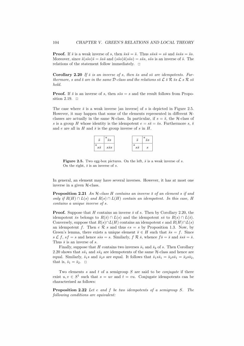
104 CHAPTER V. GREEN’S RELATIONS AND LOCAL THEORY
Proof. If s is a weak inverse of s, then sss = s. Thus ssss = ss and ssss = ss.Moreover, since s(sss)s = sss and (sss)s(sss) = sss, sss is an inverse of s. Therelations of the statement follow immediately.
Corollary 2.20 If s is an inverse of s, then ss and ss are idempotents. Fur-thermore, s and s are in the same D-class and the relations ss L s R ss L s R sshold.
Proof. If s is an inverse of s, then sss = s and the result follows from Propo-sition 2.19.
The case where s is a weak inverse [an inverse] of s is depicted in Figure 2.5.However, it may happen that some of the elements represented in different H-classes are actually in the same H-class. In particular, if s = s, the H-class ofs is a group H whose identity is the idempotent e = ss = ss. Furthermore s, sand e are all in H and s is the group inverse of s in H.
s∗ss
∗ss sss
s∗ss
∗ss s
Figure 2.5. Two egg-box pictures. On the left, s is a weak inverse of s.On the right, s is an inverse of s.
In general, an element may have several inverses. However, it has at most oneinverse in a given H-class.
Proposition 2.21 An H-class H contains an inverse s of an element s if andonly if R(H) ∩ L(s) and R(s) ∩ L(H) contain an idempotent. In this case, Hcontains a unique inverse of s.
Proof. Suppose that H contains an inverse s of s. Then by Corollary 2.20, theidempotent ss belongs to R(s) ∩ L(s) and the idempotent ss to R(s) ∩ L(s).Conversely, suppose that R(s)∩L(H) contains an idempotent e and R(H)∩L(s)an idempotent f . Then e R s and thus es = s by Proposition 1.3. Now, byGreen’s lemma, there exists a unique element s ∈ H such that ss = f . Sinces L f , sf = s and hence sss = s. Similarly, f R s, whence fs = s and sss = s.Thus s is an inverse of s.
Finally, suppose that H contains two inverses s1 and s2 of s. Then Corollary2.20 shows that ss1 and ss2 are idempotents of the same H-class and hence areequal. Similarly, s1s and s2s are equal. It follows that s1ss1 = s2ss1 = s2ss2,that is, s1 = s2.
Two elements s and t of a semigroup S are said to be conjugate if thereexist u, v ∈ S1 such that s = uv and t = vu. Conjugate idempotents can becharacterised as follows:
Proposition 2.22 Let e and f be two idempotents of a semigroup S. Thefollowing conditions are equivalent:

2. INVERSES, WEAK INVERSES AND REGULAR ELEMENTS 105
(1) e and f are conjugate,
(2) there exist two elements u, v ∈ S such that u D v D e D f , uv = e andvu = f ,
(3) e and f are D-equivalent.
Proof. It is clear that (2) implies (1) and (3).(1) implies (3). Suppose first that e = uv and f = vu for some u, v ∈ S1.
Then uvuv = uv and vuvu = vu, whence uv R uvu and uvu L vu. Thuse = uv D vu = f .
(3) implies (2). Suppose that e D f . Then there exists s ∈ S such thate R s and s L f . By Green’s lemma, there exists an element s ∈ L(e) ∩ R(f)such that ss = f . Thus sss = sf = s and sss = fs = s. It follows that s is aninverse of s. By Corollary 2.20, ss is an idempotent of the same H-class as eand thus is equal to e.
We conclude this section by an elementary result on idempotents.
Proposition 2.23 Let e be an idempotent of a semigroup S. If e = xy forsome x, y ∈ S, then ex and ye are mutually inverse elements.
Proof. Indeed, (ex)(ye)(ex) = exyex = ex and (ye)(ex)(ye) = yexye = ye.
2.2 Regular elements
An element is regular if it has at least one inverse. A semigroup is called regularif all its elements are regular. Similarly, a D-class [L-class, R-class, J -class] iscalled regular if all its elements are regular. A nonregular D-class is also calleda null D-class.
The set of regular elements of a semigroup S is denoted by Reg(S). Sincean idempotent is its own inverse, E(S) is a subset of Reg(S).
The next proposition gives various characterisations of regular elements.
Proposition 2.24 Let s be an element of a semigroup S. The following con-ditions are equivalent:
(1) s is regular,
(2) sss = s for some s ∈ S,
(3) D(s) contains an idempotent,
(4) R(s) contains an idempotent,
(5) L(s) contains an idempotent.
Proof. (1) implies (2) by definition. Condition (2) states that s is a weakinverse of s. Thus Proposition 2.19 shows that (2) implies (1), (3), (4) and (5).The equivalence of (3), (4) and (5) follows from Proposition 1.12.
(4) implies (1). Let e be an idempotent such that s R e. Then es = sand st = e for some t ∈ S1. We claim that s = tst is an inverse of s. Indeedsss = ststs = ees = es = s and sss = tststst = s. Thus s is regular.
It is useful to restate Proposition 2.24 in terms of D-classes.

106 CHAPTER V. GREEN’S RELATIONS AND LOCAL THEORY
Corollary 2.25 Let D be a D-class of a finite semigroup. The following con-ditions are equivalent:
(1) D is regular,
(2) D contains a regular element,
(3) D contains an idempotent,
(4) each R-class of D contains an idempotent,
(5) each L-class of D contains an idempotent,
(6) there exist two elements of D whose product belongs to D.
Corollary 2.25 shows that a regular D-class contains at least one idempotentin each R-class and in each L-class. It follows that all the R-classes and L-classes contained in a regular D-class are regular.
Let K be one of the Green’s relations R, L, J or H. A semigroup is K-trivialif and only if a K b implies a = b.
Proposition 2.26 Let S be a finite semigroup and let K be one of the Green’srelations R, L, H or J . Then S is K-trivial if and only if its regular K-classesare trivial.
Proof. Let n be the exponent of S.(a) K = R. Suppose x R y. Then there exist c, d ∈ S1 such that xc = y,
yd = x, whence xcd = x. One has (cd)n R (cd)nc and since the restrictionof R to the regular R-class is trivial, one gets (cd)n = (cd)nc. It follows thatx = x(cd)n = x(cd)nc = xc = y and therefore S is R-trivial.
(b) K = L. The proof is dual.(c) K = J . By (a) and (b), S is R-trivial and L-trivial. Since J = D =
R ◦ L, S is J -trivial.(d) K = H. Suppose that x H y. Then there exist a, b, c, d ∈ S1 such that
ax = y, by = x, xc = y and yd = x. It follows that x = axd and thereforeanxdn = x. Since an is idempotent and since an+1 H an, one gets an+1 = an
since the H-class of an is regular. It follows that x = anxdn = an+1xdn =a(anxdn) = ax = y. Therefore S is H-trivial.
A finiteH-trivial semigroup is also called aperiodic. See Proposition VII.4.22for more details. We conclude this section by another property of finite semi-groups.
Proposition 2.27 Let S be a finite semigroup and let T be a subsemigroup ofS. Let s ∈ T and let e be an idempotent of S. Suppose that, for some u, v ∈ T 1,e RS us, us LS s, s RS sv and sv LS e. Then e ∈ T and e RT us LT s RT
sv LT e.
e us
sv
∗
s

3. REES MATRIX SEMIGROUPS 107
Proof. Since RS(us) ∩ LS(sv) contains an idempotent, Green’s lemma showsthat svus belongs to RS(sv) ∩ LS(us), which is equal to HS(s). It follows thatthe right translation ρvus is a permutation on HS(s). Since T is finite, somepower of vus, say (vus)n is an idempotent f of T . Since ρvus is a permutationon HS(s), ρf is also a permutation on HS(s) and since f2 = f , this permutationis the identity. In particular, sf = s, that is, s(vus)n = s. It follows that s RT
sv RT svus and a dual argument shows that s LT us LT svus. Thus svus ∈RT (sv) ∩ LT (us) and by Green’s lemma again, RT (us) ∩ LT (sv) contains anidempotent. This idempotent belongs to the H-class RS(us) ∩ LS(sv), therebyit is equal to e. Thus e ∈ T .
3 Rees matrix semigroups
The Location Theorem indicates that the product of two elements s and t ofthe same D-class D either falls out of D or belongs to the intersection of theR-class of s and of the L-class of t. In the latter case, the location of st in theegg-box picture is precisely known and the intersection of the R-class of t and ofthe L-class of s is a group. This suggests that the structure of a regular D-classdepends primarily on the coordinates of its elements in the egg-box picture andon its maximal groups. This motivates the following definition.
Let I and J be two nonempty sets, G be a group and P = (pj,i)j∈J,i∈I be aJ × I-matrix with entries in G. The Rees matrix semigroup with G as structuregroup, P as sandwich matrix and I and J as indexing sets, is the semigroupM(G, I, J, P ) defined on the set I ×G× J by the operation
(i, g, j)(i′, g′, j′) = (i, gpj,i′g′, j′) (3.1)
More generally, if P = (pj,i)j∈J,i∈I is a J × I-matrix with entries in G0, we letM0(G, I, J, P ) denote the semigroup, called a Rees matrix semigroup with zero,defined on the set (I ×G× J) ∪ 0 by the operation
(i, g, j)(i′, g′, j′) =
{(i, gpj,i′g
′, j′) if pj,i′ 6= 0
0 otherwise
Example 3.1 A Brandt semigroup is a Rees matrix semigroup in which I = Jand P is the identity matrix. Therefore, the product is defined by
(i, g, j)(i′, g′, j′) =
{(i, gg′, j′) if j = i′,
0 otherwise.
A Brandt aperiodic semigroup is a Brandt semigroup whose structure group istrivial. If I = {1, . . . , n}, this semigroup is denoted by Bn. For instance, B2 isthe semigroup of 2× 2 Boolean matrices
B2 =
{(1 00 0
),
(0 10 0
),
(0 01 0
),
(0 00 1
),
(0 00 0
)}
under multiplication. This semigroup is studied in more detail in Section II.2.1.
The regularity of a Rees matrix semigroups depends only on its sandwichmatrix.
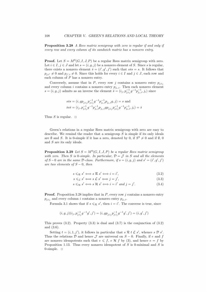
108 CHAPTER V. GREEN’S RELATIONS AND LOCAL THEORY
Proposition 3.28 A Rees matrix semigroup with zero is regular if and only ifevery row and every column of its sandwich matrix has a nonzero entry.
Proof. Let S = M0(G, I, J, P ) be a regular Rees matrix semigroup with zero.Let i ∈ I, j ∈ J and let s = (i, g, j) be a nonzero element of S. Since s is regular,there exists a nonzero element s = (i′, g′, j′) such that sss = s. It follows thatpj,i′ 6= 0 and pj′,i 6= 0. Since this holds for every i ∈ I and j ∈ J , each row andeach column of P has a nonzero entry.
Conversely, assume that in P , every row j contains a nonzero entry pj,ijand every column i contains a nonzero entry pji,i. Then each nonzero elements = (i, g, j) admits as an inverse the element s = (ij , p
−1j,ijg−1p−1
ji,i, ji) since
sss = (i, gpj,ijp−1j,ijg−1p−1
ji,ipji,ig, j) = s and
sss = (ij , p−1j,ijg−1p−1
ji,ipji,igpj,ijp
−1j,ijg−1p−1
ji,i, ji) = s
Thus S is regular.
Green’s relations in a regular Rees matrix semigroup with zero are easy todescribe. We remind the reader that a semigroup S is simple if its only idealsare ∅ and S. It is 0-simple if it has a zero, denoted by 0, if S2 6= 0 and if ∅, 0and S are its only ideals.
Proposition 3.29 Let S = M0(G, I, J, P ) be a regular Rees matrix semigroupwith zero. Then S is 0-simple. In particular, D = J in S and all the elementsof S−0 are in the same D-class. Furthermore, if s = (i, g, j) and s′ = (i′, g′, j′)are two elements of S − 0, then
s 6R s′ ⇐⇒ s R s′ ⇐⇒ i = i′, (3.2)
s 6L s′ ⇐⇒ s L s′ ⇐⇒ j = j′, (3.3)
s 6H s′ ⇐⇒ s H s′ ⇐⇒ i = i′ and j = j′. (3.4)
Proof. Proposition 3.28 implies that in P , every row j contains a nonzero entrypj,ij and every column i contains a nonzero entry pji,i.
Formula 3.1 shows that if s 6R s′, then i = i′. The converse is true, since
(i, g, j)(ij , p−1j,ijg−1g′, j′) = (i, gpj,ijp
−1j,ijg−1g′, j′) = (i, g′, j′)
This proves (3.2). Property (3.3) is dual and (3.7) is the conjunction of (3.2)and (3.6).
Setting t = (i, 1, j′), it follows in particular that s R t L s′, whence s D s′.Thus the relations D and hence J are universal on S − 0. Finally, if e and fare nonzero idempotents such that e 6 f , e H f by (3), and hence e = f byProposition 1.13. Thus every nonzero idempotent of S is 0-minimal and S is0-simple.

3. REES MATRIX SEMIGROUPS 109
j j′
i (i, g, j) (i, gpj,i′g′, j′)
i′ ∗ (i′, g′, j′)
Figure 3.6. The product of two elements when pj,i′ 6= 0.
An analogous result holds for Rees matrix semigroups.
Proposition 3.30 Let S = M(G, I, J, P ) be a Rees matrix semigroup. ThenS is simple. In particular, D and J are both the universal relation and everyH-class is a group. Furthermore, if s = (i, g, j) and s′ = (i′, g′, j′) are twoelements of S, then
s 6R s′ ⇐⇒ s R s′ ⇐⇒ i = i′, (3.5)
s 6L s′ ⇐⇒ s L s′ ⇐⇒ j = j′, (3.6)
s 6H s′ ⇐⇒ s H s′ ⇐⇒ i = i′ and j = j′. (3.7)
Proof. The proposition mostly follows from Proposition 3.29 by consideringS0. A complementary property is that s R ss′ L s′, which shows that therelations D and J are universal on S. It follows that S is simple. Taking s = s′,we get s H s2 and thus by Proposition 1.13, H(s) is a group. Consequently,each H-class is a group.
By Proposition II.3.19, a simple semigroup has a single J -class, and a 0-simple semigroup has a single nonzero J -class.
Proposition 3.31 A finite 0-simple semigroup contains a single nonzero D-class and this D-class is regular.
Proof. Let S0 be a simple semigroup. By Proposition II.3.19, S is a D-class ofS0. Furthermore, if s ∈ S, then s2 ∈ S and Corollary 1.16 shows that s H s2. Itfollows by Proposition 1.13 that H(s) is a group and thus S is a regular D-classof S0.
A similar result holds for finite simple semigroups.
Proposition 3.32 A finite simple semigroup contains a single D-class. ThisD-class is regular and each of its H-classes is a group.
We can now state the main theorem of this section.
Theorem 3.33 (Rees-Sushkevich theorem)
(1) A finite semigroup is simple if and only if it is isomorphic to some Reesmatrix semigroup.
(2) A finite semigroup is 0-simple if and only if it is isomorphic to someregular Rees matrix semigroup with zero.
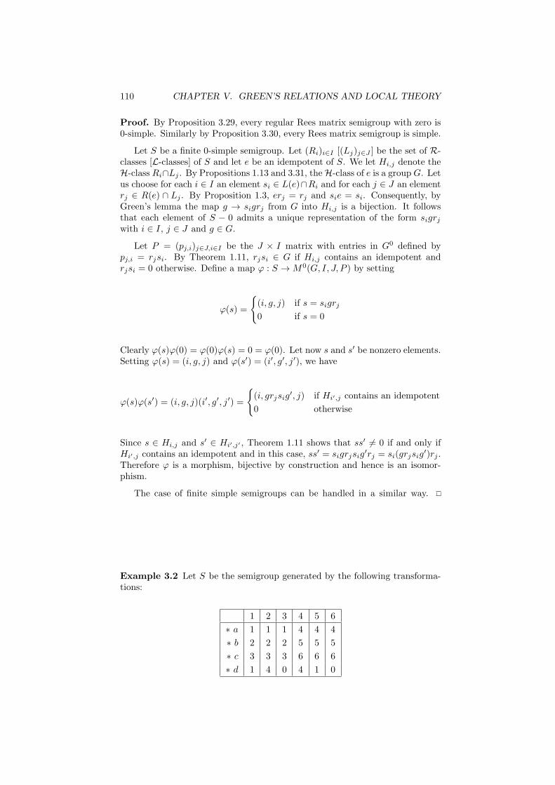
110 CHAPTER V. GREEN’S RELATIONS AND LOCAL THEORY
Proof. By Proposition 3.29, every regular Rees matrix semigroup with zero is0-simple. Similarly by Proposition 3.30, every Rees matrix semigroup is simple.
Let S be a finite 0-simple semigroup. Let (Ri)i∈I [(Lj)j∈J ] be the set of R-classes [L-classes] of S and let e be an idempotent of S. We let Hi,j denote theH-class Ri∩Lj . By Propositions 1.13 and 3.31, theH-class of e is a group G. Letus choose for each i ∈ I an element si ∈ L(e)∩Ri and for each j ∈ J an elementrj ∈ R(e) ∩ Lj . By Proposition 1.3, erj = rj and sie = si. Consequently, byGreen’s lemma the map g → sigrj from G into Hi,j is a bijection. It followsthat each element of S − 0 admits a unique representation of the form sigrjwith i ∈ I, j ∈ J and g ∈ G.
Let P = (pj,i)j∈J,i∈I be the J × I matrix with entries in G0 defined bypj,i = rjsi. By Theorem 1.11, rjsi ∈ G if Hi,j contains an idempotent andrjsi = 0 otherwise. Define a map ϕ : S →M0(G, I, J, P ) by setting
ϕ(s) =
{(i, g, j) if s = sigrj
0 if s = 0
Clearly ϕ(s)ϕ(0) = ϕ(0)ϕ(s) = 0 = ϕ(0). Let now s and s′ be nonzero elements.Setting ϕ(s) = (i, g, j) and ϕ(s′) = (i′, g′, j′), we have
ϕ(s)ϕ(s′) = (i, g, j)(i′, g′, j′) =
{(i, grjsig
′, j) if Hi′,j contains an idempotent
0 otherwise
Since s ∈ Hi,j and s′ ∈ Hi′,j′ , Theorem 1.11 shows that ss′ 6= 0 if and only ifHi′,j contains an idempotent and in this case, ss′ = sigrjsig
′rj = si(grjsig′)rj .
Therefore ϕ is a morphism, bijective by construction and hence is an isomor-phism.
The case of finite simple semigroups can be handled in a similar way.
Example 3.2 Let S be the semigroup generated by the following transforma-tions:
1 2 3 4 5 6
∗ a 1 1 1 4 4 4
∗ b 2 2 2 5 5 5
∗ c 3 3 3 6 6 6
∗ d 1 4 0 4 1 0

3. REES MATRIX SEMIGROUPS 111
The elements of S and a set of relations defining S are given below
1 2 3 4 5 6
∗ a 1 1 1 4 4 4
∗ b 2 2 2 5 5 5
∗ c 3 3 3 6 6 6
∗ d 1 4 0 4 1 0
bd 4 4 4 1 1 1
∗ cd 0 0 0 0 0 0
db 2 5 0 5 2 0
dc 3 6 0 6 3 0
bdb 5 5 5 2 2 2
bdc 6 6 6 3 3 3
dbd 4 1 0 1 4 0
∗ dbdb 5 2 0 2 5 0
dbdc 6 3 0 3 6 0
Relations:
aa = a ab = b ac = c ad = a ba = a
bb = b bc = c ca = a cb = b cc = c
da = d dd = d cd = 0 dcd = 0 bdbd = a
Finally, its D-class structure is the following:
∗a bd
∗b bdb
∗c bdc
∗d dbd
∗dbdb db dc dbdc
∗0
It follows that S is a 0-simple semigroup, isomorphic to the Rees matrix semi-group M(Z/2Z, 2, 3, P ), where Z/2Z is the multiplicative group {1,−1} and
P =
1 11 −11 0
The isomorphism is given by a = (1, 1, 1), b = (1, 1, 2), c = (1, 1, 3) and d =(2, 1, 1).
The Rees-Sushkevich theorem has some particular cases of interest. If G istrivial and Pi,j = 1 for all i ∈ I and j ∈ J , then M(I, J,G, P ) is isomorphic toa rectangular band B(I, J), which is the set I × J with the multiplication
(i, j)(k, ℓ) = (i, ℓ)
If I = {1, . . . , n} and J = {1, . . . ,m}, the notation B(n,m) is also used.

112 CHAPTER V. GREEN’S RELATIONS AND LOCAL THEORY
Corollary 3.34 Let S be a nonempty finite aperiodic semigroup. The followingconditions are equivalent:
(1) S is simple,
(2) S is idempotent and for all e, f, s ∈ S, esf = ef ,
(3) S is isomorphic to a rectangular band.
Proof. The equivalence of (1) and (3) follows directly from the Rees-Sushkevichtheorem.
(3) implies (2) since in B(I, J), (i, j)(k, ℓ)(ℓ,m) = (i,m) = (i, j)(ℓ,m).(2) implies (1). Let I be a nonempty ideal of S and let s ∈ I and e ∈ S.
Since I is an ideal, ese ∈ I. Furthermore, one has by (2), ese = ee = e. Itfollows that e ∈ I and hence I = S. Therefore S is simple.
∗
∗
∗
∗
∗
∗
∗
∗
∗
∗
∗
∗
∗
∗
∗
∗
∗
∗
∗
∗
∗
∗
∗
∗
Figure 3.7. An aperiodic simple semigroup: the rectangular band B(4, 6).
Furthermore, if I [J ] is a singleton and then M(I, J,G, P ) is a right [left] zerosemigroup. Conversely, any right [left] zero semigroup is isomorphic to such aRees matrix semigroup.
∗
∗
∗
∗ ∗ ∗ ∗
Figure 3.8. A left zero semigroup and a right zero semigroup.
4 Structure of regular D-classes
Let D be a regular D-class of a semigroup S. We define a semigroup D0 whosesupport is D ∪ 0 and multiplication (denoted by ∗) is given by
s ∗ t =
{st if st ∈ D,
0 otherwise
We then have the following proposition.
Proposition 4.35 If D is a regular D-class of a semigroup, D0 is a regular0-simple semigroup.

4. STRUCTURE OF REGULAR D-CLASSES 113
Proof. We first verify that all elements of D are D-equivalent in D0. Lets, t ∈ D and let r ∈ D be such that s R r L t. Let u and v be elements ofS1 such that r = su and s = rv. Since D is regular, L(s) [L(r)] contains anidempotent e [f ]. Thus se = s and rf = r by Proposition 1.3. It follows thatr = s(eu) and s = r(fv). Furthermore, eu L su since e L s and thus eu ∈ D.Similarly, fv ∈ D and hence s R r in D0. Dually, r L t in D0 and finally, s D tin D0.
It follows that 0 and D0 are the only ideals of D0. Thus D0 is 0-simple.Since D is regular, D0 is also regular.
An important particular case occurs when D is itself a semigroup. We sayin this case that is a full D-class of S.
Proposition 4.36 Let D be a regular D-class of a semigroup. The followingconditions are equivalent:
(1) D is full,
(2) D is a simple semigroup,
(3) every H-class of D contains an idempotent,
(4) the product of any two idempotents of D is also in D,
(5) D is isomorphic to some Rees matrix semigroup.
Proof. The equivalence of (1) and (2) is trivial and that of (2) and (5) followsfrom Theorem 3.33.
(1) implies (4) is trivial.(4) implies (3). Let H be an H-class of D and let x ∈ H. Since D is regular,
there exist by Proposition 1.12 an idempotent e in R(x) and an idemptotent fin L(x). By (4), fe belongs to D and thus, by the Location Theorem (Theorem1.11), R(e)∩L(f) contains an idempotent. But R(e)∩L(f) is equal to H, whichproves (3).
(3) implies (1) also follows from the Location Theorem.
G
...
G
G
G
...
G
G
. . .
. . .
. . .
. . .
G
...
G
G
Figure 4.9. A completely regular D-class.
4.1 Structure of the minimal ideal
Proposition 4.37 Let S be a finite semigroup. Then S has a unique minimalideal. This ideal is a regular simple semigroup.

114 CHAPTER V. GREEN’S RELATIONS AND LOCAL THEORY
Proof. The set of all ideals has a 6J -minimal element I, which is the uniqueminimal ideal of S. By construction, I is simple. Let s ∈ S. The descendingsequence s >J s2 >J s3 . . . is stationary. In particular, there exists an integern such that sn J s2n and hence sn H s2n. It follows by Proposition 1.13that H(sn) contains an idempotent. Thus E(S) is nonempty and contains a6J -minimal element e. This minimal idempotent belongs to I and thus I isregular.
It follows that the minimal ideal of a finite semigroup has the followingstructure. Every H-class is a group and all these groups are isomorphic.
∗
∗
∗
∗G
∗
∗
∗
∗
∗
∗
∗
∗
∗
∗
∗
∗
∗
∗
∗
∗
∗
∗
∗
∗
Figure 4.10. The minimal ideal of a finite semigroup.
5 Green’s relations in subsemigroups and quo-
tients
Let us start with a trivial observation: Green’s relations are stable under mor-phisms.
Proposition 5.38 Let ϕ : S → T be a morphism and let K be one of therelations 6R, 6L, 6H, 6J , R, L, H, D or J . If s K t, then ϕ(s) K ϕ(t).
Let now T be a subsemigroup [a quotient] of a semigroup S. It is oftenuseful to compare Green’s relations defined in S and T . For this purpose, if Kis any one of Green’s relations or preorders, we let KS [KT ] denote the Green’srelation or preorder defined in the semigroup S [T ].
5.1 Green’s relations in subsemigroups
We first consider the case of subsemigroups.
Proposition 5.39 Let T be a subsemigroup of a finite semigroup S and lets, t ∈ T with t regular in T . Let K be one of the relations 6R, 6L, 6H, R, Lor H. If s KS t, then s KT t.
Proof. Suppose that s 6RSt. If t is an inverse of t in T , then t RT tt and
thus s 6RStt. Since tt is idempotent, it follows from Proposition 1.3 that
tts = s. Thus s 6RTtt and finally s 6RT
t. The proof for the other relationsis similar.

5. GREEN’S RELATIONS IN SUBSEMIGROUPS AND QUOTIENTS 115
Proposition 5.39 does not extend to 6J , D nor J . Let S be, unsurprinsingly,the universal counterexample B2 = {a, b, ab, ba, 0}, with aba = a, bab = b anda2 = b2 = 0. Let T = E(S) = {ab, ba, 0}. Then ab JS ba, but ab 66JT
ba.However, if T is an ideal of S, the following property holds:
Proposition 5.40 Let T be an ideal of a finite semigroup S and let s, t ∈ Twith s or t regular in T . Let K be one of the relations 6R, 6L, 6H, 6J , R, L,H or J . If s KS t, then s KT t.
Proof. Suppose that s 6JSt. Then s = utv for some u, v ∈ S1. If s is regular,
let s be an inverse of s in T . Then s = sssss = ssutvss. Since T is an ideal,ssu and vss are elements of T . Thus s 6JT
t. If t is regular, let t be aninverse of t in T . Then s = utv = utttttv. Since T is an ideal, utt and ttv areelements of T . Thus s 6JT
t. The proof for the other relations is similar.
If T is a local subsemigroup of S (see Exercise II.10), a similar result holdswithout any regularity assumption.
Proposition 5.41 Let e be an idempotent of a finite semigroup S and let T =eSe. Let K be one of the relations 6R, 6L, 6H, 6J , R, L, H or J . If twoelements s and t of T satisfy s KS t, then s KT t.
Proof. Suppose that s 6RSt. Then s = tu for some u ∈ S1. Since s = ese
and t = ete, s = ese = etue = eeteue = eteeue = teue. Thus s 6RTt. The
proof for the other relations is similar.
A useful consequence of Proposition 5.39 is the following corollary:
Corollary 5.42 Let T be a subsemigroup of a finite semigroup S and let D bea regular DT -class of T . Then the restrictions to D of the Green’s relations inS and T coincide.
Proof. Since D is a DT -class of T , the relations DT , DS , JT and JS areuniversal on D and hence equal. The rest of the corollary follows directly fromProposition 5.39.
5.2 Green’s relations in quotient semigroups
In this subsection, ϕ will denote a surjective morphism from a semigroup S ontoa semigroup T . Little can be said in the general case.
Proposition 5.43 Let K be one of the relations R, L, H, D or J and let Kbe a KT -class of T . Then ϕ−1(K) is a union of KS-classes.
Proof. The result follows immediately from Proposition 5.38.
Stronger results hold for finite semigroups.
Proposition 5.44 Suppose that S is finite. Let J be a J -class of T and let Ibe a 6J -minimal J -class of S contained in ϕ−1(J). Then
(1) ϕ(I) = J and ϕ induces a surjective morphism from I0 onto J0,

116 CHAPTER V. GREEN’S RELATIONS AND LOCAL THEORY
(2) each R-class [L-class ] of S contained in I maps under ϕ onto an R-class[L-class ] of T contained in J ,
(3) I is regular if and only if J is regular. In this case, I is the unique minimalJ -class of ϕ−1(J).
(4) If J is null, then every J -class in ϕ−1(J) is null.
Proof. (1) First, by Proposition 5.43, ϕ−1(J) is a union of J -classes of S. SinceS is finite, there exists a 6J -minimal J -class I of S contained in ϕ−1(J).
Let s ∈ I and t ∈ J . Since ϕ(s) J t and ϕ is surjective, one has t =ϕ(u)ϕ(s)ϕ(v) for some u, v ∈ S1. Therefore ϕ(usv) = t and usv ∈ ϕ−1(J).Since s ∈ I and I is a minimal J -class in ϕ−1(J), it follows that usv ∈ I.Therefore ϕ(I) = J .
Let s, t ∈ I. If st ∈ I, then ϕ(st) ∈ J . If st /∈ I, then st <J s and henceϕ(st) /∈ J : otherwise, I would not be a minimal J -class in ϕ−1(J). Therefore,ϕ induces a well-defined surjective morphism from I0 onto J0.
(2) Let R be an R-class of I. Let r ∈ R and let t be an element of J R-equivalent to ϕ(r). Then t = ϕ(r)x for some x ∈ T 1 and since ϕ is surjective,ϕ(u) = x for some u ∈ S1. It follows that ϕ(ru) = ϕ(r)ϕ(u) = ϕ(r)x = t andtherefore ru ∈ ϕ−1(J). Since ru 6R r and I is a minimal J -class of ϕ−1(J)containing ru, one gets ru ∈ I. It follows by Theorem 1.9 that ru ∈ R and thust ∈ ϕ(R). Consequently, ϕ maps R onto an R-class of T contained in J . Theproof is dual for the L-classes.
(3) If I is regular, it contains an idempotent e. Therefore ϕ(e) is an idem-potent of J , and J is regular. Suppose now that J is regular an let e be anidempotent of J . By (1), there is an element x ∈ I such that ϕ(x) = e. Itfollows that ϕ(xω) = e and since xω 6 x and I is a 6J -minimal J -class, onegets xω ∈ I. Thus I is regular.
Let I1 and I2 be two 6J -minimal J -classes of ϕ−1(J). The previous ar-gument shows that there exist two idempotents e1 ∈ I1 and e2 ∈ I2 such thatϕ(e1) = ϕ(e2) = e. It follows that ϕ(e1e2) = e and thus e1e2 ∈ ϕ
−1(J). Butsince e1e2 6J e1 and e1e2 6J e2, one gets e1e2 ∈ J1 ∩ J2, a contradiction.
(4) is a consequence of (3) since a J -class is null if and only if it is notregular.
One says that an element y of T is lifted to an element x of S if ϕ(x) = y.Similarly, a subset Y of T is lifted to a subset X of S if ϕ(X) = Y .
Theorem 5.45 (Lifting lemma) If ϕ is a morphism from a finite semigrouponto a finite semigroup, then
(1) every idempotent lifts to an idempotent,
(2) every J -class lifts to a J -class,
(3) every regular R-class [L-class, H-class ] lifts to a regular R-class [L-class,H-class ],
(4) every group lifts to a group.
Proof. (1) has been proved several times, but we repeat the argument. If eis an idempotent of T , and x is an element of S such that ϕ(x) = e, thenϕ(xω) = e.
(2) follows from Proposition 5.44.

5. GREEN’S RELATIONS IN SUBSEMIGROUPS AND QUOTIENTS 117
(3) Let R be a regular R-class of T and let r ∈ R. Let J be the regularJ -class of T containing R. By Proposition 5.44, there is a unique 6J -minimalJ -class I of S contained in ϕ−1(J). Choose s ∈ I such that ϕ(s) = r. ByProposition 5.44 again, the R-class of s maps onto an R-class of J , which isnecessarily R. Similarly, the L-class of s maps onto the L-class of r and hence,the H-class of s maps onto the H-class of r.
(4) If H is a group of T , it is contained into a maximal group G of T whichis also an H-class. Then we may use the argument of (3) with r idempotentand we may choose by (1) s to be also idempotent. Then G lifts to an H-class containing an idempotent, which is therefore a group K. In particular, ϕinduces a group morphism from K onto G and the group ϕ−1(H) is mappedonto H. This proves that H lifts to a group.
The following example shows that Property (2) in Proposition 5.44 does notextend to H-classes.
Example 5.1 The minimal automata of the languages
K = {aibaj | i ≡ 0 mod 2 and j ≡ 0 mod 2}
L = {aibaj | i+ j ≡ 0 mod 2}
are represented in Figure 5.11:
1 2
3 4
a
a
b b
a
a
1 2
3 4
a
a
b
a
a
Figure 5.11. The minimal automata of K and L.
Their syntactic monoids M (on the left) and N (on the right) are respectively
1 1 2 3 4
a 2 1 4 3
b 3 0 0 0
ab 0 3 0 0
ba 4 0 0 0
bb 0 0 0 0
aba 0 4 0 0
1 1 2 3 4
a 2 1 4 3
b 3 4 0 0
ab 4 3 0 0
bb 0 0 0 0
The monoid M = {1, a, b, ab, ba, bab, 0} is presented on {a, b} by the relationsaa = 1, bab = 0 and bb = 0. The monoid N = {1, a, b, ab, 0} is presented on{a, b} by the relations aa = 1, ba = ab and bb = 0.
The J -class structure of M and N is represented below:

118 CHAPTER V. GREEN’S RELATIONS AND LOCAL THEORY
∗1, a
∗1, a
b ba
ab abaab, b
∗0
∗0
Let ϕ : M → N be the surjective morphism defined by ϕ(1) = 1, ϕ(a) = a,ϕ(b) = b, ϕ(ab) = ab, ϕ(ba) = ab and ϕ(aba) = b. Then J = {ab, b} is both aJ -class and an H-class of N and I = {b, ab, ba, aba} = ϕ−1(J) is a J -class ofM . However no H-class of I is mapped onto J .
6 Green’s relations and transformations
Semigroups are often given as transformation semigroups. We shall thereforeexamine the Green’s relations in such semigroups.
Given an element a ∈ T (E), we denote by Im(a) the range of a and byKer(a) the partition on E induced by the equivalence relation ∼a defined by
p ∼a q ⇐⇒ p· a = q · a
Finally, we set rank(a) = | Im(a)| = |Ker(a)|. For example, if
a =
(1 2 3 4 5 6 71 4 5 5 5 4 1
)
we have Im(a) = {1, 4, 5}, Ker(a) = 17/26/345 and rank(a) = 3.We first mention an elementary property of the rank.
Lemma 6.46 Let a, b ∈ T (E). Then rank(ab) 6 max{rank(a), rank(b)}.
Proof. This follows from the two relations Im(ab) ⊆ Im(b) and Ker(ab) ⊆Ker(a).
One can now describe the Green’s relations in the semigroup T (E).
Proposition 6.47 Let a, b be elements of T (E). Then
(1) a 6R b if and only if Ker(a) is a partition coarser than Ker(b) and a R bif and only if Ker(a) = Ker(b),
(2) a 6L b if and only if Im(a) ⊆ Im(b) and a L b if and only if Im(a) = Im(b),
(3) a 6J b if and only if rank(a) 6 rank(b) and a J b if and only if rank(a) =rank(b).
Proof. (1) If a 6R b, there exists u ∈ T (E), such that a = bu and thereforeKer(a) is coarser than Ker(b). Conversely, if this condition is satisfied, therelation u = a ◦ b−1 is a function such that bu = a. Therefore a 6R b. Theresult for R follows immediately.

6. GREEN’S RELATIONS AND TRANSFORMATIONS 119
(2) If a 6L b, there exists u ∈ T (E), such that a = ub and thereforeIm(a) ⊆ Im(b). Conversely, if Im(a) ⊆ Im(b), there exists for each q ∈ E anelement q′ such that q′ · b = q · a. The function q → q′ defines a transformationu such that ub = a and thus a 6L b. The result for L follows immediately.
(3) If a 6J b, there exist u, v ∈ T (E) such that a = ubv and thereforerank(a) 6 rank(b). Conversely, suppose that rank(a) 6 rank(b). We constructa transformation u by sending each class of Ker(a) onto an element of Im(b) andtwo distinct classes onto two distinct elements; this is possible since | Im(a)| =|Ker(a)| 6 | Im(b)|. Then Ker(u) = Ker(a) and Im(u) ⊆ Im(b) by construction.Therefore a R u by (1), u 6L b by (2) and finally a 6J u 6J b. The result forJ follows immediately.
We can now pass to the general study of transformation semigroups. Givena set E and a partition E = {E1, . . . , En} of E, we say that a subset F of E isa tranversal of E if, for 1 6 i 6 n, |Ei ∩ F | = 1.
Proposition 6.48 Let S be a subsemigroup of T (E). An element a belongs toa group of S if and only if Im(a) is a transversal of Ker(a).
Proof. If a belongs to a group, then an = a for a certain n > 2 and therefore ainduces a bijection on Im(a). Let K be a class of Ker(a). If |K∩Im(a)| > 2, twoelements of Im(a) have the same image under a, which contradicts the aboveproperty. Therefore |K ∩ Im(a)| 6 1 for every K ∈ Ker(a). Furthermore, ifK ∩ Im(a) = ∅ for a class K of Ker(a), it follows that
| Im(a)| =∑
K∈Ker(a)
|K ∩ Im(a)| < |Ker(a)|
a contradiction. Therefore Im(a) is a transversal of Ker(a).Conversely, if this condition is satisfied, a induces a bijection on its image
and therefore an = a for some n > 2. It follows by Proposition 1.13 that abelongs to a group of S.
Part of Proposition 6.47 extends to all transformation semigroups.
Proposition 6.49 Let S be a subsemigroup of T (E). Then
(1) if a 6R b, then Ker(a) is a coarser partition than Ker(b) and if a R b,then Ker(a) = Ker(b),
(2) if a 6L b, then Im(a) ⊆ Im(b) and if a L b, then Im(a) = Im(b),
(3) if a 6J b, then rank(a) 6 rank(b) and if a J b, then rank(a) = rank(b).
Proof. See the proof of Proposition 6.47.
Note that the equivalences stated in Proposition 6.47 for T (E) do not holdfor all transformation semigroups. For instance, in the semigroup S representedin Figure A.2, the elements acb and acbc have the same image but are not L-equivalent. Similarly, rank(acac) = rank(cbcb), but these two idempotents arenot J -equivalent.
However, Proposition 6.48 enables us to locate very easily the elements of agroup in S. One can then completely reconstruct the regular D-class of such anelement x by the following algorithm:

120 CHAPTER V. GREEN’S RELATIONS AND LOCAL THEORY
(1) Calculate all the sets of the form Im(xr) (where r ∈ S1) such that| Im(xr)| = | Im(x)|. For each such set I, remember an element r suchthat I = Im(xr).
(2) In parallel to (1), calculate all the transformations xr (r ∈ S1) such thatIm(xr) = Im(x). One obtains the H-class of x.
(3) Calculate all the partitions of the form Ker(sx) (where s ∈ S1) such that|Ker(sx)| = |Ker(x)|. For each such partition K, remember an element ssuch that K = Ker(sx).
(4) Among the sets calculated in (1), retain only those which are transver-sals of one of the partitions calculated in (3): one obtains a set I ={Im(xr1), . . . , Im(xrn)}, where r1 = 1. Similarly, among the partitionscalculated in (3), retain only those which admit as a transversal one ofthe sets calculated in (1). We obtain a set K = {Ker(s1x), . . . ,Ker(smx)},where s1 = 1.
(5) The results are summarised in the double-entry table below, representingthe egg-box picture of the D-class of x. If Hi,j = Rsix ∩ Lxrj , one hasHi,j = siHrj , which enables us to calculate the D-class completely. Fi-nally, the H-class Hi,j is a group if and only if Im(xrj) is a transversal ofKer(six).
H xrj
six Hi,j
smx
Im(xr1) Im(xrj) Im(xrn)
Ker(x) = Ker(s1x)
Ker(smx)
Justification of the algorithm.Recall that x is an element of a group in S. Suppose that rx R x and let
e ∈ E(S) and s ∈ S1 are such that x R xr, xr L e, e R sx and sx L x.
x xr
sx e
then by Proposition 6.48 Im(e) is a transversal of Ker(e) and by Proposition6.49, Im(e) = Im(xr) and Ker(sx) = Ker(e), so that Im(xr) is a transversal ofKer(sx). Converserly, suppose that Im(xr) is a transversal of a certain Ker(sx),where | Im(xr)| = | Im(x)| and |Ker(sx)| = |Ker(x)|. Let e ∈ T (E) be a trans-formation with range Im(xr) and with kernel Ker(sx). Then by Proposition
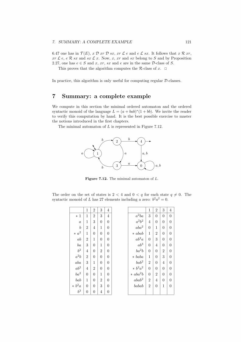
7. SUMMARY: A COMPLETE EXAMPLE 121
6.47 one has in T (E), x D xr D sx, xr L e and e L sx. It follows that x R xr,xr L e, e R sx and sx L x. Now, x, xr and sx belong to S and by Proposition2.27, one has e ∈ S and x, xr, sx and e are in the same D-class of S.
This proves that the algorithm computes the R-class of x.
In practice, this algorithm is only useful for computing regular D-classes.
7 Summary: a complete example
We compute in this section the minimal ordered automaton and the orderedsyntactic monoid of the language L = (a + bab)∗(1 + bb). We invite the readerto verify this computation by hand. It is the best possible exercise to masterthe notions introduced in the first chapters.
The minimal automaton of L is represented in Figure 7.12.
0
1
2
3
4
a, b
a
b
a
ba
a, b
b
Figure 7.12. The minimal automaton of L.
The order on the set of states is 2 < 4 and 0 < q for each state q 6= 0. Thesyntactic monoid of L has 27 elements including a zero: b2a2 = 0.
1 2 3 4
∗ 1 1 2 3 4
a 1 3 0 0
b 2 4 1 0
∗ a2 1 0 0 0
ab 2 1 0 0
ba 3 0 1 0
b2 4 0 2 0
a2b 2 0 0 0
aba 3 1 0 0
ab2 4 2 0 0
ba2 0 0 1 0
bab 1 0 2 0
∗ b2a 0 0 3 0
b3 0 0 4 0
1 2 3 4
a2ba 3 0 0 0
a2b2 4 0 0 0
aba2 0 1 0 0
∗ abab 1 2 0 0
ab2a 0 3 0 0
ab3 0 4 0 0
ba2b 0 0 2 0
∗ baba 1 0 3 0
bab2 2 0 4 0
∗ b2a2 0 0 0 0
∗ aba2b 0 2 0 0
abab2 2 4 0 0
babab 2 0 1 0

122 CHAPTER V. GREEN’S RELATIONS AND LOCAL THEORY
It is defined by the following set of relations:
a2a = a2 b2ab = ba2 b3a = 0 b4 = 0 a2ba2 = 0
a2bab = a2 a2b2a = 0 a2b3 = 0 ababa = a ab2a2 = 0
ba2ba = b2a ba2b2 = b3 baba2 = a2 bab2a = a2ba bab3 = a2b2
b2a2 = 0 babab2 = b2
It contains 7 D-classes, 15R-classes, 10 L-classes and 23H-classes. The minimalideal reduces to the zero, but there is a unique regular 0-minimal ideal. TheD-class structure is represented below:
∗1
b
∗baba ba bab babab
aba a∗abab ab
abab2
ab2
b2
bab2
∗a2 a2ba a2b
ba2∗b2a ba2b
aba2 ab2a∗aba2b
a2b2
ab3
b3
∗0
The syntactic preorder satisfies 0 < x for all x 6= 0. The other relations arerepresented below, with our usual convention: an arrow from u to v means thatu < v.

8. EXERCISES 123
1
a
b
aa
ab ba
bb
aab
aba
abbbaa
bab
bba
bbb
aaba
aabb
abaa
abab
abba
abbb baab
baba
babb
abaab
ababb
babab
8 Exercises
1. Describe Green’s relations in the syntactic monoids of Exercise IV.8.
2. Verify that in the example of Section 7, a H aba but aω 6= (aba)ω.
3. Describe Green’s relations in the following monoids:
(1) the monoid of all functions from {1, 2, 3} into itself,
(2) the monoid of all order-preserving functions from {1, 2, 3} into itself (afunction f is order-preserving if i 6 j implies f(i) 6 f(j)),
(3) the monoid of all partial functions from {1, 2, 3} into itself,
(4) the monoid of all relations on {1, 2, 3},
(5) the monoid of all reflexive relations on {1, 2, 3},
(6) the monoid of all upper-triangular Boolean matrices of size 3× 3,
(7) the monoid of all unitriangular Boolean matrices of size 3 × 3 (a matrixis unitriangular if it is upper-triangular and if its diagonal entries are allequal to 1).
4. Show that there exist finite semigroups in which none of Greens relations isa congruence.
5. Let M be a finite monoid. Let P(M) be the set of subsets of M .
(1) Show that P(M) is a monoid for the following product: given two subsetsX and Y , XY = {xy | x ∈ X, y ∈ Y }.
(2) Show that the set P1(M) of subsets of M containing 1 is a submonoid ofM . Show that this monoid is J -trivial.
6. Let s and t be regular elements of a semigroup S. Show that the followingconditions are equivalent:
(1) s R t,
(2) there exists s ∈ V (s) and t ∈ V (t) such that ss = tt,
(3) for all s ∈ V (s), there exists t ∈ V (t) such that ss = tt.
124 CHAPTER V. GREEN’S RELATIONS AND LOCAL THEORY
A dual result holds for L. Finally, show that the following conditions are equiv-alent:
(1) s H t,
(2) there exists s ∈ V (s) and t ∈ V (t) such that ss = tt and ss = tt,
(3) for all s ∈ V (s), there exists t ∈ V (t) such that ss = tt and ss = tt.
7. Let a and b be two elements of a finite semigroup. Show that if abb = b, thenbab = b.
8. Let S be a nonempty finite semigroup. Suppose that, for all a, b ∈ S, theequation ax = b has a solution and that the equation xa = b also has a solution.Show that S is a group.
9. Let S be a finite semigroup. Show that the number of inverses of an elements of S is equal to the product of the number of idempotents of the R-class of sby the number of idempotents of the L-class of s.
10. (See [65]) Show that a nonempty semigroup is a group if and only if everyelement is the weak inverse of exactly one element.
11. (See [65]) Show that a nonempty monoid is a group if and only if everyelement has exactly one weak inverse. What happens for a semigroup?
12. Let S be a regular semigroup. Show that the following conditions areequivalent:
(1) S is simple,
(2) for all s ∈ S, every weak inverse of s is also an inverse of s,
(3) for all s, t in S, if us = ut and sv = tv for some u, v ∈ S, then s = t.
13. A right group is a semigroup that is right simple and left cancellative. Provethat if G is a group and S is a right zero semigroup, then G×S is a right group.
Show that the following conditions are equivalent:
(1) S is a right group,
(2) S is right simple and contains at least one idempotent,
(3) for each s, t ∈ S, the equation ax = b has a unique solution in S,
(4) S is isomorphic to a Rees matrix semigroup M(G, I, J, P ), where |I| = 1and P is the J×I column matrix whose entries are all equal to the identityof G.
14. A monoid M is an inverse monoid if every element of M has a uniqueinverse. Show that a finite monoid is inverse if and only if M is regular (thatis, every element of M is regular) and the idempotents commute in M .
15. LetQ be a finite set and let I(Q) be the monoid of partial injective functionsfrom Q to Q under composition. Show that I(Q) is an inverse monoid and thatif M is a finite inverse monoid, then M is isomorphic to a submonoid of I(M).

9. NOTES 125
9 Notes
The material presented in this chapter can be found in almost every book onsemigroups. My favourite references are the books of Lallement [73] and Grillet[53]. More information on semigroup theory can be found in Clifford and Preston[28, 29] and Higgins [58]. The book [129] by Rhodes and Steinberg contains muchmore advanced material and Green’s relations are only treated in the appendix.We just treated the case of finite 0-simple semigroups in this chapter, but thestructure of arbitrary completely 0-simple semigroups was elucidated by Rees.
126 CHAPTER V. GREEN’S RELATIONS AND LOCAL THEORY
Chapter VI
Profinite words
The results presented in this chapter are a good illustration of the followingquotation of Marshall Stone [144]: A cardinal principle of modern mathematicalresearch may be stated as a maxim: “One must always topologize”. Indeed, amuch deeper insight into the structure of recognisable languages is made possibleby the introduction of topological concepts.
1 Topology
We start with a brief reminder of the elements of topology used in the sequel:open and closed sets, continuous functions, metric spaces, compact spaces, etc.This section is by no means a first course in topology but is simply thought asa remainder.
1.1 General topology
Recall that a topology on a set E is a set T of subsets of E satisfying the followingconditions:
(1) The empty set and E are in T ,
(2) The union of arbitrary many elements of T is an element of T ,
(3) The intersection of finitely many elements of T is an element of T .
The elements of T are called the open sets. The complement of an open set iscalled a closed set. A set is clopen if it is both open and closed.
The closure of a subset X of E, denoted by X, is the intersection of theclosed sets containing X. A subset of E is dense if its closure is equal to E.
A topological space is a set E together with a topology on E. A topology T2on a set is a refinement of a topology T1 on the same set, if each open set forT1 is also an open set for T2. One also says that T1 is coarser than T2 or thatT2 is stronger than T1.
The coarsest topology on E is the trivial topology, which reduces to theempty set and E. The strongest topology is the discrete topology defined byT = P(E).
If F is a subset of a topological space (E, T ), then the traces F ∩ X forX ∈ T , define a topology on F , called the relative topology.
127
128 CHAPTER VI. PROFINITE WORDS
It is sometimes convenient to give a basis for a topology on E. This is acollection B of subsets of E such that every open set is the union of elementsof B. Thus B is a basis for some topology on E if it satisfies the two followingconditions:
(i) E is the union of all the elements of B,
(ii) every finite intersection of elements of B is a union of elements of B.
The open sets of the topology generated by B are by definition the arbitraryunions of elements of B.
A map from a topological space into another one is continuous if the inverseimage of each open set is an open set. It is an homeomorphism if it is a con-tinuous bijection and the inverse bijection is also continuous. Two topologicalspaces are homeomorphic if there is an homeomorphism between them.
Let (Ei, Ti)i∈I be a family of topological spaces, and let E =∏
i∈I Ei bethe cartesian product of the Ei’s. Denote by πi the natural projection from Eonto Ei, defined by πi((ej)j∈I) = ei. The product topology on E is the topologygenerated by the basis consisting of the finite intersections of sets of the formπ−1i (Xi) where Xi is an open set of Ei. These sets are nothing else than the
products∏
i∈I Xi where the Xi’s are open sets of Ei and where Xi = Ei exceptfor a finite number of indices. The natural projections πi : E → Ei are thencontinuous and a mapping ϕ : F → E is continuous if and only if the mappingsπi ◦ ϕ : F → Ei, for i ∈ I, are all continuous.
A topological space (E, T ) is Hausdorff if for each u, v ∈ E with u 6= v,there exist disjoint open sets U and V such that u ∈ U and v ∈ V . If f is acontinuous map from a topological space X into an Hausdorff space Y , then thegraph of f is closed in X × Y .
1.2 Metric spaces
A metric d on a set E is a map d : E × E → R+ from E × E into the setof nonnegative real numbers satisfying the following three conditions, for everyx, y, z ∈ E:
(1) d(x, y) = 0 if and only if x = y,
(2) d(y, x) = d(x, y),
(3) d(x, z) 6 d(x, y) + d(y, z)
A metric space is a set E together with a metric d on E.The topology defined by d is obtained by taking as a basis the open ε-balls
defined for x ∈ E and ε > 0 by
B(x, ε) = {y ∈ E | d(x, y) < ε}
Every metric space is Hausdorff. Indeed, given two distinct elements x and y,the open balls B(x, ε) and B(y, ε) are disjoint if ε is set to be half the distancebetween x and y.
A sequence (xn)n>0 of elements of a metric space (E, d) is converging to alimit x if, for each ε > 0, there exists an integer k such that for each n > k,d(xn, x) < ε. A sequence is said to be convergent if it admits a limit.
Limits are convenient when characterising other topological properties ofmetric spaces. For instance, a subset F of E is closed if and only if, for everysequence (xn)n>0 of elements of F converging to a limit x, x itself belongs to

1. TOPOLOGY 129
F . A map ϕ : (E, d)→ (E′, d′) between two metric spaces is continuous if andonly if, for every sequence (xn)n>0 of elements of E converging to a limit x, thesequence (ϕ(xn))n>0 converges to ϕ(x).
A Cauchy sequence in a metric space (E, d) is a sequence (xn)n>0 of elementsof E such that for each ε > 0, there exists an integer k such that for each n > kand m > k, d(xn, xm) < ε. Every convergent sequence is a Cauchy sequence,but the converse does not hold in general. A metric space in which each Cauchysequence is convergent is said to be complete. Every closed subset of a completespace is complete.
Let (Ei, di)16i6n be a finite family of metric spaces. Then (E1×· · ·×En, d)is a metric space, where d, defined by
d((x1, . . . , xn), (y1, . . . , yn)) = max{d(x1, y1), . . . , d(xn, yn)}
is a metric that defines the product topology.Let (E, d) and (E′, d′) be two metric spaces. A function ϕ from E into
E′ is said to be uniformly continuous if for each ε > 0, there exists δ > 0such that the relation d(x, y) < δ implies d′(ϕ(x), ϕ(y)) < ε. If ϕ is uniformlycontinuous, the image under ϕ of a Cauchy sequence of E is a Cauchy sequenceof E′. We say that ϕ is a uniform homeomorphism if it is a uniformly continuousbijection and ϕ−1 is also uniformly continuous. Two metric spaces are uniformlyhomeomorphic if there is a uniform homeomorphism between them.
We say that ϕ is an isometry if it is a bijection from E onto E′ such that,for each x, y ∈ E,
d(x, y) = d′(ϕ(x), ϕ(y))
The completion of a metric space E is a complete metric space E together withan isometric embedding of E as a dense subspace of E. One can prove that everymetric space admits a completion, which is unique up to isometric equivalence:if E1 and E2 are two completions of E, there exists an isometry of E1 onto E2,whose restriction to E is the identity.
The completion of E can be constructed as follows. Let C(E) be the set ofCauchy sequences in E. Define an equivalence relation ∼ on C(E) as follows.Two Cauchy sequences x = (xn)n>0 and y = (yn)n>0 are equivalent if theinterleaved sequence x0, y0, x1, y1, . . . is also a Cauchy sequence. The completionof E is defined to be the set E of equivalence classes of C(E). The metric d on
E extends to a metric on E defined by
d(x, y) = limn→∞
d(xn, yn)
where x and y are representative Cauchy sequences of elements in E. Thedefinition of the equivalence ensures that the above definition does not dependon the choice of x and y in their equivalence class and the fact that R is completeensures that the limit exists.
1.3 Compact spaces
An important notion is that of compact space. A family of open sets (Ui)i∈I
is said to cover a topological space (E, T ) if E =⋃
i∈I Ui. A topological space(E, T ) is said to be compact if for each family of open sets covering E, thereexists a finite subfamily that still covers E.

130 CHAPTER VI. PROFINITE WORDS
Compact metric spaces admit two important characterisations. First, a met-ric space is compact if and only if every sequence has a convergent subsequence.Second, a metric space is compact if and only if it is complete and totallybounded, which means that, for every n > 0, the space can be covered by afinite number of open balls of radius < 2−n. Furthermore, a metric space istotally bounded if and only if its completion is totally bounded. Therefore ametric space is totally bounded if and only if its completion is compact.
If X is a closed set of a compact space E, then X, equipped with the relativetopology, is also a compact space. We shall use freely the well-known result thatevery product of compact spaces is compact (Tychonov’s theorem).
One can show that if ϕ : E → F is a continuous map from a topologicalspace E into a topological Hausdorff space F , the image of a compact set underϕ is still compact. Moreover if E is a compact metric space and F is a metricspace, then every continuous function from E to F is uniformly continuous.
We conclude this section with a useful extension result that is worth to bestated separately.
Proposition 1.1 Let E and F be metric spaces. Any uniformly continuousfunction ϕ : E → F admits a unique uniformly continuous extension ϕ : E → F .Furthermore, if E is compact and if ϕ is surjective, then ϕ is surjective.
In particular, if F is complete, any uniformly continuous function from E to Fadmits a unique uniformly continuous extension from E to F .
1.4 Topological semigroups
A topological semigroup is a semigroup S equipped with a topology for which thesemigroup operation is continuous. This means that the function from S × Sinto S which maps (x, y) onto xy is continuous. A compact semigroup is atopological semigroup which is compact as a topological space.
2 Profinite topology
2.1 The free profinite monoid
Let A be a finite alphabet. A morphism ϕ : A∗ → M separates two words uand v of A∗ if ϕ(u) 6= ϕ(v). By extension, we say that a monoid M separatestwo words if there is a morphism from A∗ onto M that separates them.
Example 2.1
(1) The words ababa and abaa can be separated by a group of order 2. Indeed,let π : A∗ → Z/2Z be the morphism defined by π(x) = |x| (mod 2). Thenπ(ababa) = 1 and π(abaa) = 0 and hence π separates u and v.
(2) More generally, two words u and v of unequal length can be separated bya finite cyclic group. Indeed, suppose that |u| < |v| and let n = |v|. Letπ : A∗ → Z/nZ be the morphism defined by π(x) = |x| (mod n). Thenπ(v) = 0 but π(u) 6= 0. Note that u and v can also be separated by a finitemonoid of size |u|+2. Define an addition ⊕ on M = {0, 1, . . . , |u|+1} bys ⊕ t = min{s + t, |u| + 1} and let ϕ : A∗ → M be the morphism definedby ϕ(x) = min{|x|, |u|+ 1}. Then ϕ(u) = |u| and ϕ(v) = |u|+ 1.
2. PROFINITE TOPOLOGY 131
(3) A similar idea can be applied if the number of occurrences of some lettera is not the same in u and v. Assume for instance that |u|a < |v|a and letn = |v|a. Then the morphism π : A∗ → Z/nZ defined by π(a) = 1 andπ(c) = 0 for c 6= a separates u and v.
(4) Recall (see Section II.2.2) that the monoid U2 is defined on the set {1, a, b}by the operation aa = ba = a, bb = ab = b and 1x = x1 = x for allx ∈ {1, a, b}. Let u and v be words of {a, b}∗. Then the words ua and vbcan be separated by the morphism π : A∗ → U2 defined by π(a) = a andπ(b) = b since π(ua) = a and π(ub) = b.
These examples are a particular case of a general result.
Proposition 2.2 Any pair of distinct words of A∗ can be separated by a finitemonoid.
Proof. Let u and v be two distinct words of A∗. Since the language {u} isrecognisable, there exists a morphism ϕ from A∗ onto a finite monoid M whichrecognises it, that is, such that ϕ−1(ϕ(u)) = {u}. It follows that ϕ(v) 6= ϕ(u)and thus ϕ separates u and v.
We now define a metric on A∗ with the following intuitive idea in mind: twowords are close for this metric if a large monoid is required to separate them.Let us now give the formal definition. Given two words u, v ∈ A∗, we set
r(u, v) = min {|M | |M is a monoid that separates u and v}
d(u, v) = 2−r(u,v)
with the usual conventions min ∅ = +∞ and 2−∞ = 0.Thus d(u, v) < 2−n if and only if u and v cannot be separated by a monoid
of size 6 n and d(x, y) < ε if and only if x and y cannot be separated by amonoid of size < n, where n is the smallest positive integer such that 2−n < ε.
The following proposition establishes the main properties of d.
Proposition 2.3 The function d is an ultrametric, that is, satisfies the follow-ing properties, for all u, v, w ∈ A∗,
(1) d(u, v) = 0 if and only if u = v,
(2) d(u, v) = d(v, u),
(3) d(u,w) 6 max{d(u, v), d(v, w)}.
It also satisfies the property
(4) d(uw, vw) 6 d(u, v) and d(wu,wv) 6 d(u, v).
Proof. (1) follows from Proposition 2.2.(2) is trivial.(3) Let M be a finite monoid separating u and w. Then M separates either
u and v, or v and w. It follows that min(r(u, v), r(v, w)) 6 r(u,w) and henced(u,w) 6 max{d(u, v), d(v, w)}.
(4) A finite monoid separating uw and vw certainly separates u and v. There-fore d(uw, vw) 6 d(u, v) and, dually, d(wu,wv) 6 d(u, v).
Thus (A∗, d) is a metric space, but it is not very interesting as a topologicalspace.
132 CHAPTER VI. PROFINITE WORDS
Proposition 2.4 The topology defined on A∗ by d is discrete: every subset isclopen.
Proof. Let u be a word of A∗ and let n be the size of the syntactic monoidM of the language {u}. Then if d(u, v) < 2−n, r(u, v) > n and in particular,M does not separate u and v. It follows that u = v. Therefore the open ballB(u, 2−n) is equal to {u}. It follows that every singleton is open. Now if U isa language of A∗, one has U =
⋃u∈U{u} and hence U is open. For the same
reason, U c is open and thus every subset of A∗ is clopen.
The completion of (A∗, d), denoted by A∗, is much more interesting. Itselements are called the profinite words on the alphabet A.
Theorem 2.5 The set of profinite words A∗ is compact.
Proof. Suppose that A is finite. Since A∗ is complete, it suffices to verify that,for every n > 0, A∗ is covered by a finite number of open balls of radius < 2−n.Consider the congruence ∼n defined on A∗ by
u ∼n v if and only if ϕ(u) = ϕ(v) for every morphism ϕ
from A∗ onto a monoid of size 6 n.
Since A is finite, there are only finitely many morphisms from A∗ onto a monoidof size 6 n, and thus ∼n is a congruence of finite index. Furthermore, d(u, v) <2−n if and only if u and v cannot be separated by a monoid of size 6 n, i.e.they are ∼n-equivalent. It follows that the ∼n-classes are open balls of radius< 2−n and cover A∗.
The density of A∗ in A∗ has several useful consequences, which are sum-marised in the next propositions. We first establish an important property ofthe product.
Proposition 2.6 The function (u, v) → uv from A∗ × A∗ to A∗ is uniformlycontinuous.
Proof. By Proposition 2.3, one has for all u, u′, v, v′ ∈ A∗,
d(uv, u′v′) 6 max{d(uv, uv′), d(uv′, u′v′)} 6 max{d(v, v′), d(u, u′)}
which proves the result.
It follows from Proposition 1.1 that the product on A∗ can be extendedin a unique way, by continuity, to A∗. Since the formulas (xy)z = x(yz) and1x = x = x1 are preserved by passage to the limit, this extended product is alsoassociative and admits the empty word as identity element. The product on A∗
is also uniformly continuous and makes A∗ a topological monoid. It is calledthe free profinite monoid because it satisfies a universal property comparable tothat of A∗. Before stating this universal property precisely, let us state anotheruseful consequence of the density of A∗.
Proposition 2.7 Every morphism ϕ from A∗ into a discrete finite monoid Mis uniformly continuous and can be extended (in a unique way) to a uniformly
continuous morphism ϕ from A∗ into M .
2. PROFINITE TOPOLOGY 133
Proof. If d(u, v) < 2−|M |, then ϕ does not separate u and v and hence ϕ(u) =ϕ(v). It follows that ϕ is a uniformly continuous function from A∗ into the dis-crete metric spaceM . Therefore ϕ has a unique uniformly continuous extensionϕ from A∗ into M . It remains to prove that ϕ is a morphism. Let
D = {(u, v) ∈ A∗ × A∗ | ϕ(uv) = ϕ(u)ϕ(v)}
We claim that D = A∗ × A∗, which exactly says that ϕ is a morphism. Wealready have ϕ(uv) = ϕ(u)ϕ(v) for u, v ∈ A∗ since ϕ is a morphism, and thus
D contains A∗ × A∗. Since A∗ × A∗ is dense in A∗ × A∗, it suffices to provethat D is closed, which essentially follows from the uniform continuity of theproduct. In more details, let π : A∗×A∗ → A∗ be the map defined by π(u, v) =uv. Proposition 2.6 shows that π is uniformly continuous and has a uniquecontinuous extension π from A∗ × A∗ to A∗ (the product on A∗). With thisnotation in hand, we get
ϕ(uv) = (ϕ ◦ π)(u, v) and ϕ(u)ϕ(v) = (π ◦ (ϕ× ϕ))(u, v)
It follows that
D =⋃
m∈M
(ϕ ◦ π)−1(m) ∩ (π ◦ (ϕ× ϕ))−1(m)
Since ϕ ◦ π and π ◦ (ϕ × ϕ) are both continuous and {m} is a closed subset ofM , it follows that D is closed, which concludes the proof.
However, there are some noncontinuous morphisms from A∗ onto a finitemonoid. For instance, the morphism ϕ : A∗ → U1 defined by
ϕ(u) =
{1 if u ∈ A∗
0 otherwise
is not continuous since ϕ−1(1) = A∗ is not closed. Now, the restriction of ϕ to
A∗, which is continuous, has a continuous extension to A∗. But this extensionmaps every profinite word to 1 and is therefore not equal to ϕ.
2.2 Universal property of the free profinite monoid
We are ready to state the universal property of A∗.
Proposition 2.8 If ϕ is a function from A into a finite monoid M , there existsa unique (uniformly) continuous monoid morphism ϕ : A∗ → M such that, foreach a ∈ A, ϕ(a) = ϕ(a). Moreover, ϕ is surjective if and only if the set ϕ(A)generates M .
Proof. First, there exists by Proposition II.5.28 a unique morphism from A∗
into M which extends ϕ and by Proposition 2.7, a unique uniformly continuousmorphism ϕ from A∗ into M that extends ϕ.
One has ϕ(A∗) ⊆ ϕ(A∗). Since M is discrete, it follows that ϕ is surjectiveif and only if ϕ(A) generates M .

134 CHAPTER VI. PROFINITE WORDS
One can also use Proposition 2.7 to define directly the metric on A∗. Let ussay that a morphism ϕ from A∗ onto a finite monoid M separates two profinitewords u and v of A∗ if ϕ(u) 6= ϕ(v).
Given two profinite words u, v ∈ A∗, we set
r(u, v) = min {|M | |M is a finite monoid that separates u and v}
d(u, v) = 2−r(u,v)
with the usual conventions min ∅ = +∞ and 2−∞ = 0.The term profinite is justified by the following property, which often serves
as a definition in the literature.
Proposition 2.9 The profinite topology on A∗ is the least topology which makescontinuous every morphism from A∗ onto a finite discrete monoid.
Proof. Proposition 2.7 shows that every morphism from A∗ onto a finite dis-crete monoid is continuous for the topology defined by d.
Suppose now that A∗ is equipped with a topology T such that every mor-phism from A∗ onto a finite discrete monoid is continuous. We claim that forall ε > 0 and for all x ∈ A∗, the ball
B(x, ε) = {y ∈ A∗ | d(x, y) < ε}
is open in T . First observe that d(x, y) < ε if and only if x and y cannot beseparated by a monoid of size < n, where n is the smallest positive integer suchthat 2−n < ε. It follows that B(x, ε) is the intersection of the sets ϕ−1(ϕ(x)),where ϕ runs over the set of all morphisms from A∗ onto a monoid of size < n.By assumption on T , each set of the form ϕ−1(ϕ(x)) is open and since A isfinite, there are finitely many morphisms from A∗ onto a monoid of size < n.This proves the claim and the proposition.
What about sequences? First, every profinite word is the limit of a Cauchysequence of words. Next, a sequence of profinite words (un)n>0 is convergingto a profinite word u if and only if, for every morphism ϕ from A∗ onto a finitemonoid, ϕ(un) is ultimately equal to ϕ(u).
2.3 ω-terms
It is relatively difficult to give “concrete” examples of profinite words which arenot words. One such example is the profinite word xω, associated with everyprofinite word x. The formal definition is
xω = limn→∞
xn!
and is justified by the following result, which shows that the sequence xn! hasindeed a limit in A∗.
Proposition 2.10 For each x ∈ A∗, the sequence (xn!)n>0 is a Cauchy se-
quence. It converges to an idempotent element of A∗.
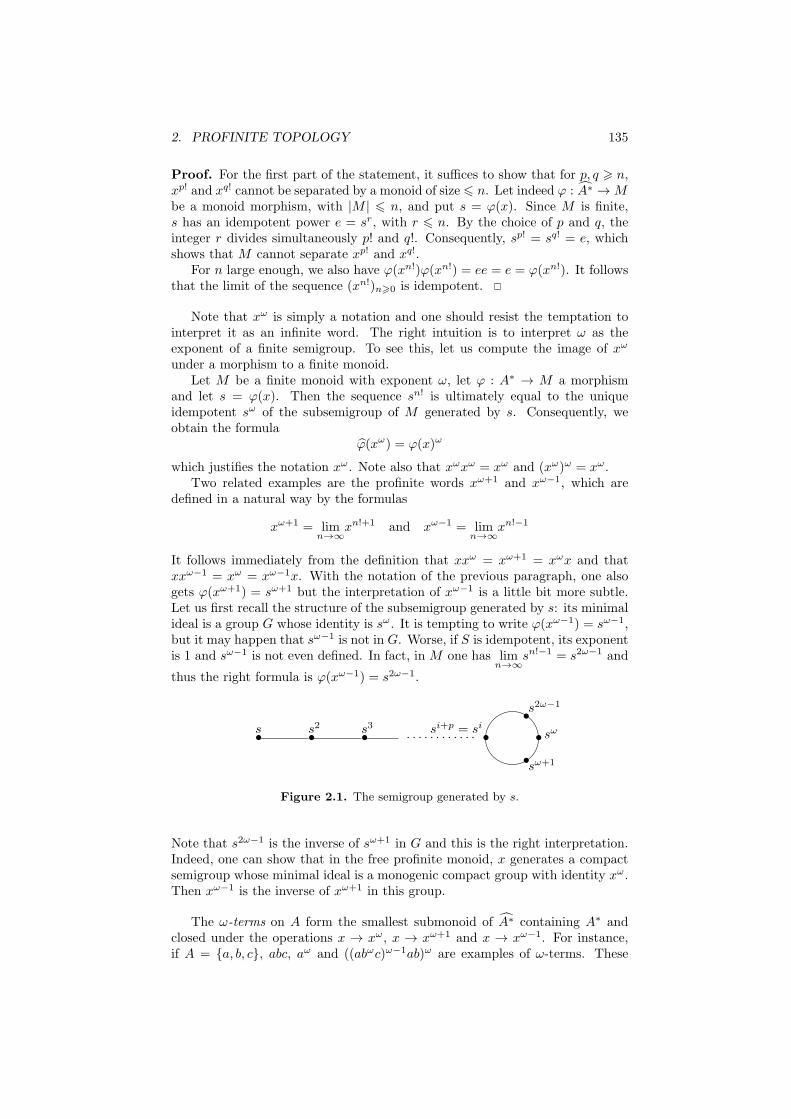
2. PROFINITE TOPOLOGY 135
Proof. For the first part of the statement, it suffices to show that for p, q > n,xp! and xq! cannot be separated by a monoid of size 6 n. Let indeed ϕ : A∗ →Mbe a monoid morphism, with |M | 6 n, and put s = ϕ(x). Since M is finite,s has an idempotent power e = sr, with r 6 n. By the choice of p and q, theinteger r divides simultaneously p! and q!. Consequently, sp! = sq! = e, whichshows that M cannot separate xp! and xq!.
For n large enough, we also have ϕ(xn!)ϕ(xn!) = ee = e = ϕ(xn!). It followsthat the limit of the sequence (xn!)n>0 is idempotent.
Note that xω is simply a notation and one should resist the temptation tointerpret it as an infinite word. The right intuition is to interpret ω as theexponent of a finite semigroup. To see this, let us compute the image of xω
under a morphism to a finite monoid.Let M be a finite monoid with exponent ω, let ϕ : A∗ → M a morphism
and let s = ϕ(x). Then the sequence sn! is ultimately equal to the uniqueidempotent sω of the subsemigroup of M generated by s. Consequently, weobtain the formula
ϕ(xω) = ϕ(x)ω
which justifies the notation xω. Note also that xωxω = xω and (xω)ω = xω.Two related examples are the profinite words xω+1 and xω−1, which are
defined in a natural way by the formulas
xω+1 = limn→∞
xn!+1 and xω−1 = limn→∞
xn!−1
It follows immediately from the definition that xxω = xω+1 = xωx and thatxxω−1 = xω = xω−1x. With the notation of the previous paragraph, one alsogets ϕ(xω+1) = sω+1 but the interpretation of xω−1 is a little bit more subtle.Let us first recall the structure of the subsemigroup generated by s: its minimalideal is a group G whose identity is sω. It is tempting to write ϕ(xω−1) = sω−1,but it may happen that sω−1 is not in G. Worse, if S is idempotent, its exponentis 1 and sω−1 is not even defined. In fact, in M one has lim
n→∞sn!−1 = s2ω−1 and
thus the right formula is ϕ(xω−1) = s2ω−1.
•s
•s2
•s3 . . . . . . . . . . . .si+p = si
•
s2ω−1
•
sω•
sω+1•
Figure 2.1. The semigroup generated by s.
Note that s2ω−1 is the inverse of sω+1 in G and this is the right interpretation.Indeed, one can show that in the free profinite monoid, x generates a compactsemigroup whose minimal ideal is a monogenic compact group with identity xω.Then xω−1 is the inverse of xω+1 in this group.
The ω-terms on A form the smallest submonoid of A∗ containing A∗ andclosed under the operations x → xω, x → xω+1 and x → xω−1. For instance,if A = {a, b, c}, abc, aω and ((abωc)ω−1ab)ω are examples of ω-terms. These

136 CHAPTER VI. PROFINITE WORDS
ω-terms represent the most intuitive examples of profinite words, but unfortu-nately, there are way more profinite words than ω-terms. To be precise, the freeprofinite monoid A∗ is uncountable (even on a one letter alphabet!) while theset of ω-terms is countable.
3 Recognisable languages and clopen sets
There is a strong connexion between recognisable and clopen subsets. We startby considering the recognisable subsets of A∗.
Proposition 3.11 Let P be a subset of A∗ and let M be its syntactic monoid.The following conditions are equivalent:
(1) P is clopen,
(2) the syntactic congruence of P is a clopen subset of A∗ × A∗,
(3) P is recognisable and its syntactic morphism is a continuous map from
A∗ onto the discrete finite space M .
Proof. Let ∼P denote the syntactic congruence of P and by η : A∗ → M itssyntactic morphism. Recall that s ∼P t if, for all u, v ∈ A∗, the conditionsusv ∈ P and utv ∈ P are equivalent.
(1) implies (2). It follows from the definition of ∼P that
∼P =⋂
u,v∈A∗
((u−1Pv−1 × u−1Pv−1) ∪ (u−1P cv−1 × u−1P cv−1)
)(3.1)
If P is clopen, each set u−1Pv−1 is also clopen. Indeed, u−1Pv−1 is the inverseimage of the clopen set P under the continuous function x 7→ uxy. Now, Formula(3.1) shows that ∼P is closed.
In order to show that the complement of ∼P is closed, consider a sequence(sn, tn) of elements of (∼P )
c, converging to a limit (s, t). Since sn 6∼P tn, thereexist some profinite words un, vn such that unsnvn ∈ P and untnvn /∈ P . SinceA∗ × A∗ is compact, the sequence (un, vn) has a convergent subsequence. Let(u, v) be its limit. Since both P and P c are closed and since the multiplication
in A∗ is continuous, one gets usv ∈ P and utv /∈ P . Therefore, s 6∼P t, whichshows that (∼P )
c is closed. Thus ∼P is clopen.
(2) implies (3). If ∼P is clopen, then for each s ∈ A∗, there exists an openneighborhood U of s such that U × U ⊆ ∼P . Therefore U is contained in the∼P -class of s. This proves that the ∼P -classes form an open partition of A∗.By compactness, this partition is finite and thus P is recognisable. Moreover,since each ∼P -class is open, the syntactic morphism of P is continuous.
(3) implies (1). Let π : A∗ → M be the syntactic morphism of P . SinceP is recognisable, M is finite. One has P = π−1(π(P )) and since M is finite,
π(P ) is clopen in M . Finally, since π is continuous, P is clopen in A∗.
We now turn to languages of A∗.
Proposition 3.12 If L is a language of A∗, then L = L ∩ A∗. Furthermore,the following conditions are equivalent:
3. RECOGNISABLE LANGUAGES AND CLOPEN SETS 137
(1) L is recognisable,
(2) L = K ∩A∗ for some clopen subset K of A∗,
(3) L is clopen in A∗,
(4) L is recognisable in A∗.
Proof. The inclusion L ⊆ L ∩ A∗ is obvious. Let u ∈ L ∩ A∗ and let M bethe syntactic monoid of {u}. Since M separates u from any word v differentfrom u, one gets r(u, v) 6 |M | if u 6= v. Let (un)n∈N be a sequence of wordsof L converging to u. If d(un, u) < 2−|M |, one has necessarily u = un and thusu ∈ L.
(1) implies (2). If L is recognisable, there is a morphism ϕ from A∗ onto afinite monoid M such that L = ϕ−1(ϕ(L)). Let K = ϕ−1(ϕ(L)). Since M isdiscrete, ϕ(L) is a clopen subset ofM and since ϕ is continuous, K is also clopen.Moreover, ϕ and ϕ coincide on A∗ and thus L = ϕ−1(ϕ(L)) ∩A∗ = K ∩A∗.
(2) implies (3). Suppose that L = K ∩ A∗ with K clopen. Since K is open
and A∗ is dense in A∗, K ∩ A∗ is dense in K. Thus L = K ∩A∗ = K. Thus Lis clopen in A∗.
(3) implies (4) follows from Proposition 3.11.
(4) implies (1). Let η : A∗ → F be the syntactic morphism of L and letP = η(L). Let η be the restriction of η to A∗. Then we have L = L ∩ A∗ =η−1(P ) ∩A∗ = η−1(P ). Thus L is recognisable.
We now describe the closure in A∗ of a recognisable language of A∗.
Proposition 3.13 Let L be a recognisable language of A∗ and let u ∈ A∗. Thefollowing conditions are equivalent:
(1) u ∈ L,
(2) ϕ(u) ∈ ϕ(L), for all morphisms ϕ from A∗ onto a finite monoid,
(3) ϕ(u) ∈ ϕ(L), for some morphism ϕ from A∗ onto a finite monoid thatrecognises L,
(4) η(u) ∈ η(L), where η is the syntactic morphism of L.
Proof. (1) implies (2). Let ϕ be a morphism from A∗ onto a finite monoid
F and let ϕ be its continuous extension to A∗. Then ϕ(L) ⊆ ϕ(L) since ϕ iscontinuous, and ϕ(L) = ϕ(L) = ϕ(L) since F is discrete. Thus if u ∈ L, thenϕ(u) ∈ ϕ(L).
(2) implies (4) and (4) implies (3) are trivial.(3) implies (1). Let ϕ be a morphism from A∗ onto a finite monoid F .
Let un be a sequence of words of A∗ converging to u. Since ϕ is continuous,ϕ(un) converges to ϕ(u). But since F is discrete, ϕ(un) is actually ultimatelyequal to ϕ(u). Thus for n large enough, one has ϕ(un) = ϕ(u). It followsby (3) that ϕ(un) = ϕ(un) ∈ ϕ(L) and since ϕ recognises L, we finally getun ∈ ϕ
−1(ϕ(L)) = L. Therefore u ∈ L.
Corollary 3.14 Let L be a recognisable language of A∗ and let η be its syntacticmorphism. Then L = η−1(η(L)).
Let Clopen(A∗) denote the Boolean algebra of all clopen sets of A∗.
138 CHAPTER VI. PROFINITE WORDS
Theorem 3.15 The maps L 7→ L and K 7→ K ∩ A∗ define mutually inverseisomorphisms between the Boolean algebras Rec(A∗) and Clopen(A∗). In par-ticular, the following formulas hold, for all L,L1, L2 ∈ Rec(A∗):
(1) Lc = (L)c,
(2) L1 ∪ L2 = L1 ∪ L2,
(3) L1 ∩ L2 = L1 ∩ L2.
Proof. Property (1) follows from Proposition 3.13. Indeed, let η be the syn-tactic morphism of L. Then since L = η−1(η(L)) and Lc = η−1(η(L)c), one hasη(Lc) = η(L)c. Therefore, one gets the following sequence of equalities:
Lc = η−1(η(Lc)) = η−1(η(L)c) = [η−1(η(L))]c = (L)c
Property (2) is a general result of topology and (3) is a consequence of (1) and(2).
Theorem 3.15 shows that the closure operator behaves nicely with respectto Boolean operations. It also behaves nicely for the left and right quotientsand for inverses of morphisms.
Proposition 3.16 Let L be a recognisable language of A∗ and let x, y ∈ A∗.Then x−1Ly−1 = x−1Ly−1.
Proof. Let η be the syntactic morphism of L. Since η also recognises x−1Ly−1,Proposition 3.13 can be used twice to get
u ∈ x−1Ly−1 ⇐⇒ η(u) ∈ η(x−1Ly−1)⇐⇒ η(x)η(u)η(y) ∈ η(L)
⇐⇒ η(xuy) ∈ η(L)⇐⇒ xuy ∈ L⇐⇒ u ∈ x−1Ly−1
which gives the result.
Proposition 3.17 Let ϕ : A∗ → B∗ be a morphism of monoids and L be arecognisable language of B∗. Then ϕ−1(L) = ϕ−1(L).
Proof. Let η be the syntactic morphism of L and let N = η ◦ ϕ(A∗). Then Nis a submonoid of M and the surjective morphism η ◦ ϕ : A∗ → N recognisesϕ−1(L). Using Proposition 3.13 and observing that η ◦ ϕ = η ◦ ϕ, we have onthe one hand
u ∈ ϕ−1(L)⇐⇒ ϕ(u) ∈ L⇐⇒ η(ϕ(u)) ∈ η(L) ∩N ⇐⇒ η ◦ ϕ(u) ∈ η(L) ∩N
Using again Proposition 3.13, and observing that ϕ(ϕ−1(L)) = L ∩ ϕ(A∗) weget on the other hand
u ∈ ϕ−1(L)⇐⇒ η ◦ ϕ(u) ∈ η(ϕ(ϕ−1(L))⇐⇒ η ◦ ϕ(u) ∈ η(L ∩ ϕ(A∗))
Now, by Proposition IV.2.6, η(L∩ϕ(A∗)) = η(L)∩ η(ϕ(A∗)) = η(L)∩N . Thusthe two conditions u ∈ ϕ−1(L) and u ∈ ϕ−1(L) are equivalent, which concludesthe proof.
4. EXERCISES 139
4 Exercises
1. A metric d on a space E is said to be an ultrametric if, for every x, y, z ∈ E,d(x, z) 6 max{d(x, y), d(y, z)}. Show that if d(x, y) 6= d(y, z), then d(x, z) =max{d(x, y), d(y, z)}. Show that any open ball B(x, ε) is clopen and that forany y ∈ B(x, r), B(x, r) = B(y, r).
5 Notes
Profinite algebra goes back at least to Birkhoff [14, p. 52-53], where he intro-duces topologies defined by congruences on abstract algebras. Profinite topolo-gies for free groups were subsequently explored by M. Hall [54] and is now animportant branch of group theory. The profinite approach has also been usedto much profit in semigroup theory and in automata theory, in particular byReutenauer [127] and by Almeida, who greatly developed the theory [1, 3, 4].In particular, Almeida’s book [3] is a major reference. See also the survey ofWeil [163].

140 CHAPTER VI. PROFINITE WORDS

Chapter VII
Varieties
The definition of a variety of finite monoids is due to Eilenberg [40]. It is inspiredby the definition of a Birkhoff variety of monoids (see Exercise 1) which appliesto infinite monoids, while Eilenberg’s definition is restricted to finite monoids.The word “variety” was coined after the term used in algebraic geometry todesignate the solutions of a set of algebraic equations. This is no coincidence:a theorem of Birkhoff states that a Birkhoff variety can be described by a set ofidentities (see Exercise 2). The counterpart of Birkhoff’s theorem for varietiesof finite monoids was obtained by Reiterman [126] and independently by Ba-naschewski [9]. The statement is exactly the same: any variety of finite monoidscan be described by a set of identities, but the definition of an identity is nowdifferent! For Birkhoff, an identity is a formal equality between words, but forReiterman, it is a formal equality between profinite words. One must alwaystopologize. . .
Warning. Since we are mostly interested in finite semigroups, the semigroupsand monoids considered in this chapter are either finite or free, except in Exer-cises 1 and 2.
1 Varieties
A variety of semigroups is a class of semigroups V such that:
(1) if S ∈ V and if T is a subsemigroup of S, then T ∈ V,
(2) if S ∈ V and if T is a quotient of S, then T ∈ V,
(3) if (Si)i∈I is a finite family of semigroups of V, then∏
i∈I Si is also in V.
Conditions (1) and (2) can be replaced by a single condition: if S ∈ V and if Tdivides S, then T ∈ V. Therefore, a variety of semigroups can be defined as aclass of semigroups closed under division and finite products.
A more subtle point: condition (3) can be replaced by the conjunction ofconditions (4) and (5):
(4) the trivial semigroup 1 belongs to V,
(5) if S1 and S2 are semigroups of V, then S1 × S2 is also in V.
Indeed, condition (4) is obtained by taking I = ∅ in (3).
Example 1.1
141

142 CHAPTER VII. VARIETIES
(1) The class S of all semigroups forms a variety of semigroups.
(2) The smallest variety of semigroups is the trivial variety, consisting of theempty semigroup and of the semigroup with one element 1. This varietyis denoted by 1.
Varieties of monoids, varieties of ordered semigroups and varieties of orderedmonoids are defined in the same way: it suffices to replace every occurrence ofsemigroup by monoid [ordered semigroup, ordered monoid ] in the definition.We shall sometimes use the term “variety” as a shorthand for variety of semi-groups [monoids, etc.]. Examples of varieties are deferred to Section ??.
Let C be a class of monoids [semigroups, ordered monoids, ordered semi-groups]. The intersection of all varieties containing C is a variety, called thevariety generated by C and denoted by 〈C〉. The next proposition provides amore explicit description.
Proposition 1.1 A monoid belongs to 〈C〉 if and only if it divides a finiteproduct of monoids of C.
Proof. Let V be the class of all monoids dividing a finite product of monoidsof C. Since a variety is closed under division and finite product, every monoid ofV belongs to 〈C〉. Therefore, it suffices to prove that V is a variety. PropositionII.3.14 shows that V is closed under product and Proposition II.3.9 shows thatV is closed under division. Thus V is a variety.
The supremum of two varieties V1 and V2 is the variety generated by V1
and V2. It is denoted by V1 ∨V2. A direct application of Proposition 1.1 givesthe following characterisation.
Corollary 1.2 A monoid belongs to V1 ∨V2 if and only if it divides a monoidof the form M1 ×M2, with M1 ∈ V1 and M2 ∈ V2.
2 Free pro-V monoids
We introduced the free profinite monoid A∗ in Section VI.2. A similar notion,the free pro-V monoid, can be defined for each variety of monoids [semigroups]V.
A monoid M separates two words u and v of the free monoid A∗ if thereexists a morphism ϕ from A∗ ontoM such that ϕ(u) 6= ϕ(v). Let V be a varietyof monoids. We set
rV(u, v) = min{Card(M) M is a monoid of V that separates u and v }
and dV(u, v) = 2−rV(u,v), with the usual conventions min ∅ = +∞ and 2−∞ = 0.We first establish some general properties of dV.
Proposition 2.3 The following properties hold for every u, v, w ∈ A∗
(1) dV(u, v) = dV(v, u)
(2) dV(uw, vw) 6 dV(u, v) and dV(wu,wv) 6 dV(u, v)
(3) dV(u,w) 6 max{dV(u, v), dV(v, w)}

2. FREE PRO-V MONOIDS 143
Proof. The first assertion is trivial. A monoid of V separating uw and vwcertainly separates u and v. Therefore dV(uw, vw) 6 dV(u, v), and dually,dV(wu,wv) 6 dV(u, v).
Let M be a monoid of V separating u and w. Then M separates either uand v, or v and w. It follows that min(rV(u, v), rV(v, w)) 6 rV(u,w) and hencedV(u,w) 6 max{dV(u, v), dV(v, w)}.
In the general case, dV is not always a metric, because one may havedV(u, v) = 0 even if u 6= v. For instance, if V is the variety of commuta-tive monoids, dV(ab, ba) = 0, since there is no way to separate ab and ba by acommutative monoid. To work around this difficulty, we first observe that, byProposition 2.3, the relation ∼V defined by
u ∼V v if and only if dV(u, v) = 0
is a congruence on A∗. Then Proposition VI.2.6 can be generalised as follows.
Proposition 2.4
(1) The function dV is an ultrametric on A∗/∼V.
(2) The product on A∗/∼V is uniformly continuous for this metric.
Proof. (1) follows directly from Proposition 2.3, since dV(u, v) = 0 impliesu ∼V v by definition. We use the same proposition to obtain the relation
dV(uv, u′v′) 6 max{dV(uv, uv′), dV(uv′, u′v′)} 6 max{dV(v, v′), dV(u, u′)}
which proves (2).
The completion of the metric space (A∗/∼V, dV) is denoted by FV(A) andcalled the free pro-V monoid on A. Its main properties are presented in the nextthree propositions. Let πV be the natural morphism from A∗ onto A∗/∼V.
Proposition 2.5 The following properties hold for each finite alphabet A:
(1) The monoid FV(A) is compact.
(2) There is a unique surjective uniformly continuous morphism from A∗ onto
FV(A) extending πV.
Proof. (1) Since FV(A) is complete, it suffices to verify that, for every n > 0,A∗ is covered by a finite number of open balls of radius < 2−n. Consider thecongruence ∼n defined on A∗ by
u ∼n v if and only if ϕ(u) = ϕ(v) for every morphism ϕ from A∗
onto a monoid of size 6 n of V.
Since A is finite, there are only finitely many morphisms from A∗ onto a monoidof size 6 n, and thus ∼n is a congruence of finite index. Furthermore, dV(u, v) <2−n if and only if u and v cannot be separated by a monoid of V of size 6 n,i.e. are ∼n-equivalent. It follows that the ∼n-classes are open balls of radius< 2−n and cover A∗.
(2) Since dV(u, v) 6 d(u, v), πV is uniformly continuous, and since A∗ iscompact, Proposition VI.1.1 shows that it can be extended (in a unique way)
to a uniformly continuous morphism from A∗ onto FV(A).
The monoid FV(A) has the following universal property:

144 CHAPTER VII. VARIETIES
Proposition 2.6 For each mapping ϕ from A into a monoid M of V, thereis a unique uniformly continuous morphism ϕ : FV(A) → M such that, for alla ∈ A, ϕ(a) = ϕ(πV(a)).
Proof. Let ϕ be a continuous morphism from A∗ into a monoidM of V. Up toreplacingM by ϕ(A∗), we may assume that ϕ is surjective. Since A∗ is dense in
A∗, andM is discrete, the restriction of ϕ to A∗ is also surjective. Furthermore,since u ∼V v implies ϕ(u) = ϕ(v), Proposition II.3.22 shows that there is asurjective morphism π from A∗/∼V onto M such that ϕ = π ◦ πV. We claimthat this morphism is uniformly continuous. Indeed if dV(u, v) < 2−|M |, thenu and v cannot be separated by M , and hence ϕ(u) = ϕ(v). Since A∗/∼V is
dense in FV(A), π can be extended by continuity to a surjective morphism from
FV(A) onto M . Thus M is a quotient of FV(A).
Proposition 2.7 A finite A-generated monoid belongs to V if and only if it isa continuous quotient of FV(A).
Proof. IfM is an A-generated monoid of V, there exists a surjective morphismϕ from A∗ onto M . Following the argument used in the proof of Proposition2.6, if dV(u, v) < 2−|M |, then ϕ(u) = ϕ(v), and thus ϕ is uniformly continuouswith respect to dV. By Proposition VI.1.1, ϕ can be extended to a uniformlycontinuous morphism from FV(A) onto M .
Conversely, assume thatM is a finite quotient of FV(A) and let π : FV(A)→M be a surjective morphism. The set
D = {(u, v) ∈ FV(A)× FV(A) | π(u) = π(v)}
is the inverse image under π of the diagonal of M ×M , and since M is discreteand π is continuous, it is a clopen subset of FV(A)× FV(A). Let F be the class
of all morphisms from FV(A) onto a monoid of V. For each ϕ ∈ F , let
Cϕ = {(u, v) ∈ FV(A)× FV(A) | ϕ(u) 6= ϕ(v)}
Each Cϕ is open by continuity of ϕ. Furthermore, if (u, v) does not belongto any Cϕ, then u and v cannot be separated by any monoid of V and hencedV(u, v) = 0, which gives u = v and π(u) = π(v). It follows that the family
D ∪ (Cϕ)ϕ∈F is a covering of FV(A) × FV(A) by open sets, and since FV(A)is compact, it admits a finite subcovering, say D ∪ (Cϕ)ϕ∈F . Therefore, ifϕ(u) = ϕ(v) for each ϕ ∈ F , then π(u) = π(v). Consequently M is a quotient
of a submonoid of the finite monoid∏
ϕ∈F ϕ(FV(A)) and thus belongs to V.
Given a variety V, it is in general a hard problem to describe the structureof FV(A). However, if V is generated by a single monoid M , then FV(A) hasa simple structure. Let MA be the set of all functions from A to M . Eachfunction ϕ : A→M extends in a unique way to a monoid morphism from A∗ to
M , also denoted by ϕ. Denote by MMA
the monoid of all functions from MA
to M under pointwise multiplication.For each letter a ∈ A, let a be the function from MA to M defined by
a(ϕ) = ϕ(a). This defines a function a 7→ a from A into MMA
, which can be

3. IDENTITIES 145
extended to a morphism u 7→ u from A∗ into MMA
. We claim that, for anyfunction ϕ : A → M , one has u(ϕ) = ϕ(u) for each word u ∈ A∗. Indeed, ifu = a1 · · · an, one gets by definition
u(ϕ) = a1(ϕ) · · · an(ϕ) = ϕ(a1) · · ·ϕ(an) = ϕ(u)
The image of A∗ under the map u 7→ u is a submonoid F of MMA
.
Proposition 2.8 If V is generated by a single monoid M , then FV(A) is equal
to F . In particular, FV(A) is a submonoid of MMA
and hence is finite.
Proof. It suffices to prove that u ∼V v is equivalent to u = v. Recall thatu ∼V v if and only if, for each morphism ϕ : A∗ → N , where N ∈ V, one hasϕ(u) = ϕ(v).
Suppose that u ∼V v and let ϕ : A → M be a function, which extendsto a morphism from A∗ to M . Since M ∈ V, one has ϕ(u) = ϕ(v) and thusu(ϕ) = v(ϕ). It follows that u = v.
Suppose now that u = v and let ϕ be a morphism from A∗ onto a monoidN of V. Since V is generated by M , N divides a power of M . Therefore thereexist a positive integer n, a submonoid T of Mn and a surjective morphismπ : T → N . By Corollary II.5.30, there exists a morphism α : A∗ → T suchthat ϕ = π ◦α. Denoting by πi the i-th projection fromMn ontoM and settingαi = πi ◦ α, we get α(u) = (α1(u), . . . , αn(u)). Now since αi is a morphismfrom A∗ to M , one has αi(u) = u(αi). Since u = v, it follows that α(u) = α(v)and finally ϕ(u) = ϕ(v). Therefore u ∼V v, which concludes the proof.
A variety such that FV(A) is finite for each alphabet A is called locallyfinite. It is tempting to guess, in view of Proposition 2.8, that every locallyfinite variety is generated by a single monoid. However, this is not the case:one can show that the variety of idempotent monoids is locally finite but notfinitely generated.
3 Identities
3.1 What is an identity?
Let A be a finite alphabet and let u and v be two profinite words of A∗. Amonoid M satisfies the profinite identity u = v if, for each monoid morphismϕ : A∗ → M , one has ϕ(u) = ϕ(v). Similarly, an ordered monoid (M,6)satisfies the profinite identity u 6 v if, for each monoid morphism ϕ : A∗ →M ,one has ϕ(u) 6 ϕ(v). An identity u = v [u 6 v] where u and v are words issometimes called an explicit identity.
One can give similar definitions for [ordered] semigroups, by taking twononempty profinite words u and v. A semigroup S satisfies the identity u = v if,for each semigroup morphism ϕ : A+ → S, one has ϕ(u) = ϕ(v) [ϕ(u) 6 ϕ(v)].The context is usually sufficient to know which kind of identities is considered.In case of ambiguity, one can utilise the more precise terms [ordered ] monoididentity or [ordered ] semigroup identity.
Formally, a profinite identity is a pair of profinite words. But in practice,one often thinks directly in terms of elements of a monoid. Consider for instance
146 CHAPTER VII. VARIETIES
the explicit identity xy3z = yxyzy. A monoid M satisfies this identity if, foreach morphism γ : {x, y, z}∗ → M , one has γ(xy3z) = γ(yxyzy). Settingγ(x) = s, γ(y) = t and γ(z) = u, this can be written as st3u = tstut. Since thisequality should hold for any morphism γ, it is equivalent to require that, for alls, t, u ∈ M , one has st3u = tstut. Now, the change of variables is unnecessary,and one can write directly that M satisfies the identity xy3z = yxyzy if andonly if, for all x, y, z ∈ M , one has xy3z = yxyzy. Similarly, a monoid iscommutative if it satisfies the identity xy = yx.
It is also possible to directly interpret any ω-term in a finite semigroup[monoid] S. As it was already mentioned, the key idea is to think of ω asthe exponent of S. For instance, an identity like xωyω = yωxω can be readilyinterpreted by saying that idempotents commute in S. The identity xωyxω = xω
means that, for every e ∈ E(S) and for every s ∈ S, ese = e. Propositions 4.23and 4.27 provide other enlighting examples.
3.2 Properties of identities
Let us now state some elementary but important properties of identities. Weconsider identities of ordered monoids, but the result can be readily adapted tothe other types of identities.
Proposition 3.9 Let u and v be profinite words on the alphabet A and let Mbe an ordered monoid satisfying the identity u 6 v. Then for all x, y ∈ A∗, Msatisfies the identity xuy 6 xvy. Furthermore, for each morphism γ : A∗ → B∗,M satisfies the identity γ(u) 6 γ(v).
Proof. Let ϕ : A∗ →M be a monoid morphism. Since M satisfies the identityu 6 v, one has ϕ(u) 6 ϕ(v). Since ϕ is a morphism, it follows that ϕ(xuy) 6
ϕ(xvy) for all x, y ∈ A∗. Therefore, M satisfies the identity xuy 6 xvy.Let γ : A∗ → B∗ and α : B∗ →M be morphisms. Then α ◦ γ is a morphism
from A∗ into M . Since M satisfies the identity u 6 v and since α ◦ γ = α ◦ γ,one has α(γ(u)) 6 α(γ(v)). Therefore M satisfies the identity γ(u) 6 γ(v).
It is a common practice to implicitly use the second part of Proposition 3.9without giving the morphism γ explicitly, but simply by substituting a profiniteword for a letter. For instance, one can prove that the monoid identity
xyx = x (3.1)
implies the identity x2 = x by taking y = 1 in (3.1). Similarly, the identityxωyxω = xω implies the identity xω+1 = xω by taking y = x, since xωxxω =xωxωx = xωx.
3.3 Reiterman’s theorem
Given a set E of profinite identities, the class of monoids [semigroups, orderedmonoids, ordered semigroups] defined by E is the class of all monoids [semi-groups, ordered monoids, ordered semigroups] satisfying all the identities of Eand is denoted by JEK.

3. IDENTITIES 147
The main result of this section, Reiterman’s theorem (Theorem 3.13), statesthat varieties can be characterised by profinite identities. We first establish theeasy part of this result.
Proposition 3.10 Let E be a set of identities. Then JEK is a variety ofmonoids [semigroups, ordered monoids, ordered semigroups ].
Proof. We treat only the case of ordered monoids, but the other cases aresimilar. Since varieties are closed under intersection, it suffices to prove theresult when E consists of a single identity, say u 6 v. Let M be an orderedmonoid satisfying this identity. Clearly, every submonoid of M satisfies thesame identity.
Let N be a quotient of M and let π :M → N be a surjective morphism. Weclaim that N also satisfies u 6 v. Indeed, if ϕ : A∗ → N is a morphism, thereexists by Corollary II.5.30 a morphism ψ : A∗ →M such that ϕ = π◦ψ. SinceMsatisfies the identity u 6 v, one gets ψ(u) 6 ψ(v) and thus π(ψ(u)) 6 π(ψ(v)).
Finally, since ϕ = π ◦ ψ, one obtains ϕ(u) 6 ϕ(v), which proves the claim.
Finally, let (Mi)i∈I be a finite family of ordered monoids satisfying the iden-tity u 6 v. We claim that their product M =
∏i∈I Mi also satisfies this
identity. Indeed, let πi denote the projection from M onto Mi and let ϕ be amorphism from A∗ into M . Since πi ◦ ϕ is a morphism from A∗ into Mi andsince πi ◦ ϕ = πi ◦ ϕ, one has πi ◦ ϕ(u) 6 πi ◦ ϕ(v). As this holds for eachi, one has ϕ(u) 6 ϕ(v). This proves the claim and concludes the proof.
A variety V satisfies a given identity if every monoid of V satisfies thisidentity. We also say in this case that the given identity is an identity of V.Identities of V are closely related to free pro-V monoids.
Proposition 3.11 Let A be a finite alphabet. Given two profinite words u andv of A∗, u = v is an identity of V if and only if πV(u) = πV(v).
Proof. If u = v is an identity of V, then u and v cannot be separated by anymonoid of V. Thus dV(u, v) = 0, u ∼V v and πV(u) = πV(v). Converselyif πV(u) = πV(v), then by Proposition 2.5, ϕ(u) = ϕ(v) for every continuous
morphism ϕ from A∗ into a monoid of V, and thus u = v is an identity of V.
Corollary 3.12 Let V and W be two varieties of monoids satisfying the sameidentities on the alphabet A. Then FV(A) and FW(A) are isomorphic.
In particular, an identity of a monoid of V can be given as a pair (u, v)
of elements of FV(A). Given a set E of identities, let JEK denote the classof monoids satisfying all the identities of E. Reiterman’s theorem states thatthese classes are exactly the varieties of monoids [semigroups, ordered monoids,ordered semigroups].
Theorem 3.13 (Reiterman) A class of [ordered ] monoids [semigroups ] is avariety if and only if it can be defined by a set of profinite identities.
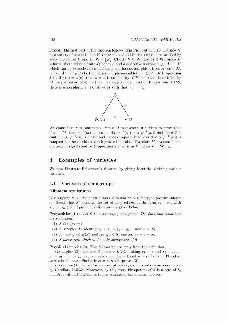
148 CHAPTER VII. VARIETIES
Proof. The first part of the theorem follows from Proposition 3.10. Let now Vbe a variety of monoids. Let E be the class of all identities which are satisfied byevery monoid of V and let W = JEK. Clearly V ⊆W. Let M ∈W. Since Mis finite, there exists a finite alphabet A and a surjective morphism ϕ : A∗ →Mwhich can be extended to a uniformly continuous morphism from A∗ onto M .Let π : A∗ → FV(A) be the natural morphism and let u, v ∈ A∗. By Proposition3.11, if π(u) = π(v), then u = v is an identity of V and thus, is satisfied byM . In particular, π(u) = π(v) implies ϕ(u) = ϕ(v) and by Proposition II.3.22,
there is a morphism γ : FV(A)→M such that γ ◦ π = ϕ.
FV(A) M
A∗
π
γ
ϕ
We claim that γ is continuous. Since M is discrete, it suffices to prove thatif m ∈ M , then γ−1(m) is closed. But γ−1(m) = π(ϕ−1(m)) and since ϕ iscontinuous, ϕ−1(m) is closed and hence compact. It follows that π(ϕ−1(m)) iscompact and hence closed which proves the claim. Therefore M is a continuousquotient of FV(A) and by Proposition 2.7, M is in V. Thus V = W.
4 Examples of varieties
We now illustrate Reiterman’s theorem by giving identities defining variousvarieties.
4.1 Varieties of semigroups
Nilpotent semigroups
A semigroup S is nilpotent if it has a zero and Sn = 0 for some positive integern. Recall that Sn denotes the set of all products of the form s1 · · · sn, withs1, . . . , sn ∈ S. Equivalent definitions are given below.
Proposition 4.14 Let S be a nonempty semigroup. The following conditionsare equivalent:
(1) S is nilpotent,
(2) S satisfies the identity x1 · · ·xn = y1 · · · yn, where n = |S|,
(3) for every e ∈ E(S) and every s ∈ S, one has es = e = se,
(4) S has a zero which is the only idempotent of S.
Proof. (1) implies (2). This follows immediately from the definition.(2) implies (3). Let s ∈ S and e ∈ E(S). Taking x1 = s and x2 = . . . =
xn = y1 = . . . = yn = e, one gets s = e if n = 1 and se = e if n > 1. Thereforese = e in all cases. Similarly es = e, which proves (3).
(3) implies (4). Since S is a nonempty semigroup, it contains an idempotentby Corollary II.6.32. Moreover, by (3), every idempotent of S is a zero of S,but Proposition II.1.2 shows that a semigroup has at most one zero.

4. EXAMPLES OF VARIETIES 149
(4) implies (1). Denote by 0 the zero of S. Then by Corollary II.6.35,Sn = SE(S)S = S{0}S = 0.
Nilpotent semigroups form a variety, denoted by N, and defined by theidentities xωy = xω = yxω.
Lefty and righty trivial semigroups
A semigroup is called lefty [righty ] trivial if, for every idempotent e of S, thesemigroup eS [Se] is trivial. Equivalently, e is a left [right] zero of S, that is,for every s ∈ S, one has es = e [se = e]. Equivalent definitions are possible:
Proposition 4.15 Let S be a nonempty semigroup and let I be its minimalideal. Let n = |S|. The following conditions are equivalent:
(1) S is lefty trivial,
(2) I is a left zero semigroup and is equal to E(S),
(3) I is a left zero semigroup and Sn = I,
(4) S satisfies the identity x1 · · ·xnx = x1 · · ·xn.
Proof. (1) implies (2). Let s ∈ I. Then for every e ∈ E(S), one has e = es ∈ Isince I is an ideal and therefore E(S) ⊆ I. Moreover if e ∈ E(S) and s, t ∈ S1,(set)(set) = se(tset) = se = set since e is a left zero of S. It follows thatE(S) is a nonempty ideal of S contained in I and hence E(S) = I since I isminimal. Furthermore, since every idempotent of S is a left zero, I is a left zerosemigroup.
(2) implies (3). By Corollary II.6.35, Sn = SE(S)S. If I = E(S), this givesSn = SIS = I.
(3) implies (4). Suppose that (3) holds and let x, x1, . . . , xn ∈ S. Thenx1 · · ·xn ∈ I and since I is an ideal, x1 · · ·xnx ∈ I. Now since I is a left zerosemigroup,
x1 · · ·xn = (x1 · · ·xn)(x1 · · ·xnx) = (x1 · · ·xn)(x1 · · ·xn)x = (x1 · · ·xn)x
which proves (4).(4) implies (1). Let s ∈ S and e ∈ E(S). Taking x = s and x1 = . . . = xn =
e, one gets es = e and hence S is lefty trivial.
Note that, in a lefty trivial semigroup, all regular elements are in the minimalideal. Furthermore, all nonregular D-classes are trivial. Let us state the dualresult for the righty trivial semigroups.
Proposition 4.16 Let S be a nonempty semigroup and let I be its minimalideal. Let n = |S|. The following conditions are equivalent:
(1) S is righty trivial,
(2) I is a right zero semigroup and is equal to E(S),
(3) I is a right zero semigroup and Sn = I,
(4) S satisfies the identity xx1 · · ·xn = x1 · · ·xn.
The lefty [righty] trivial semigroups form a variety of finite semigroups, de-noted by ℓ1 [r1], and defined by the identity xωy = xω [yxω = xω]. For historicalreasons, a different notation is often used in the literature. The variety ℓ1 isdenoted by K and the variety r1 by D.

150 CHAPTER VII. VARIETIES
∗
...
∗
∗
◦
◦◦
◦◦
◦ ◦
◦
◦◦
◦◦
◦ ◦
Nonregular elements
Minimal ideal
∗ ∗ . . . ∗
Figure 4.1. A lefty trivial semigroup (on the left) and a righty trivialsemigroup (on the right).
Locally trivial semigroups
A semigroup is called locally trivial if for every s ∈ S and e ∈ E(S), ese = e.Equivalent definitions are given below.
Proposition 4.17 Let S be a nonempty semigroup and let n = |S|. The fol-lowing conditions are equivalent:
(1) S is locally trivial,
(2) the minimal ideal of S is equal to E(S),
(3) for every e, f ∈ E(S) and every s ∈ S, one has esf = ef ,
(4) S satisfies the identity x1 · · ·xnxx1 · · ·xn = x1 · · ·xn.
Proof. (1) implies (2). Let s ∈ I. Then for every e ∈ E(S), one has e = ese ∈ Isince I is an ideal and therefore E(S) ⊆ I. Moreover if e ∈ E(S) and s, t ∈ S1,(set)(set) = se(ts)et = set and thus set is idempotent. It follows that E(S) isa nonempty ideal of S contained in I and hence E(S) = I.
(2) implies (3). Suppose that I = E(S). Then I is an aperiodic semigroup,which is also simple by Proposition V.4.37. Let s ∈ S and let e, f ∈ E(S).Then e, f, esf ∈ I since I is an ideal. It follows by Corollary V.3.34 thatesf = eesff = e(esf)f = ef .
(3) implies (4). By Corollary II.6.35, Sn = SE(S)S. Let x, x1, . . . , xn ∈ S.Then x1 · · ·xn ∈ S
n and hence x1 · · ·xn = set for some s, t ∈ S and e ∈ E(S).It follows by (3)
x1 · · ·xnxx1 · · ·xn = (set)x(set) = s(etxse)t = set = x1 · · ·xn

4. EXAMPLES OF VARIETIES 151
which gives (4).(4) implies (1). Let s ∈ S and e ∈ E(S). Taking x = s and x1 = . . . = xn =
e, one gets ese = e and hence S is locally trivial.
Thus the locally trivial semigroups form a variety of finite semigroups, denotedby L1, and defined by the identity xωyxω = xω.
Locally groups
A semigroup is locally a group if for every e ∈ E(S), the semigroup eSe is agroup. Equivalent definitions are given below.
Proposition 4.18 Let S be a nonempty semigroup. The following conditionsare equivalent:
(1) S is locally a group,
(2) every idempotent of S belongs to the minimal ideal of S,
(3) S satisfies the identity (xωyxω)ω = xω,
Proof. Let I be the minimal ideal of S and let n be the exponent of S.(1) implies (2). Let s ∈ I and let e ∈ E(S). Since eSe is a group whose
identity is e, one has (ese)n = e. Now, I is an ideal and thus e ∈ I. It followsthat E(S) is a subset of I.
(2) implies (3). Suppose that E(S) ⊆ I. By Proposition V.4.37, I is a simplesemigroup. Let s ∈ S and let e ∈ E(S). Since I is an ideal, one has e, ese ∈ Iand thus e J ese. Since ese 6R e and ese 6L e, Theorem V.1.9 shows thatese H e. Therefore (ese)n = e and S satisfies the identity (xωyxω)ω = xω.
(3) implies (1). Let s ∈ S and e ∈ E(S). Taking x = e and y = s, one gets(ese)ω = e, which shows that S is locally a group.
Semigroups which are locally a group form a variety of finite semigroups, de-noted by LG and defined by the identity (xωyxω)ω = xω.
Simple semigroups
Proposition 4.19 A semigroup is simple if and only if it satisfies the identitiesxω+1 = x and (xyx)ω = xω.
Proof. Let S be a simple semigroup. By Proposition V.3.32, S has a singleD-class, which is a union of groups. Let x, y ∈ S. One has xω+1 6H x and(xyx)ω 6H x and hence by Theorem V.1.9 (3) and (4), xω+1 H x and (xyx)ω Hxω. It follows immediately that (xyx)ω = xω since an H-class contains a uniqueidempotent and xω+1 = x since xω is the identity of the H-class containing xand xω+1.
Conversely, suppose that S satisfies the two identities
xω+1 = x and (xyx)ω = xω
The first identity shows that every element x is H-equivalent to xω and to xω+1
and hence belongs to the maximal group whose identity is xω. In particular,all the elements of S are regular. Furthermore, if x, y ∈ S, one has x J xω =(xyx)ω 6J xyx 6J y. It follows that x 6J y and by duality y 6J x. It followsthat all elements of S are J -equivalent.
Simple semigroups form a variety of semigroups, usually denoted by CS.

152 CHAPTER VII. VARIETIES
4.2 Varieties of monoids
Groups
The next proposition shows that groups form a variety of monoids, denoted byG.
Proposition 4.20 The class of all groups is a variety of monoids, defined bythe identity xω = 1.
Proof. Finite groups are closed under quotients and finite direct products andit follows from Proposition II.3.13 that a submonoid of a group is a group.
Since a monoid is a group if and only if its unique idempotent is 1, theidentity xω = 1 characterises the variety of finite groups.
Subvarieties of G include the variety Gcom of commutative groups and,for each prime number p, the variety Gp of p-groups. Recall that a group is ap-group if its order is a power of p.
Commutative monoids
A monoid is commutative if and only if it satisfies the identity xy = yx. There-fore, the commutative monoids form a variety of monoids, denoted by Com.
Proposition 4.21 Every commutative monoid divides the product of its mono-genic submonoids.
Proof. LetM be a commutative monoid and let N be the product of its mono-genic submonoids. Let ϕ : N → M be the morphism which transforms eachelement on N into the product of its coordinates. Then ϕ is clearly surjectiveand thus M is a quotient of N .
Aperiodic monoids
A monoid M is aperiodic if there is an integer n > 0 such that, for all x ∈ M ,xn = xn+1. Since we assume finiteness, quantifiers can be inverted in thedefinition: M is aperiodic if for each x ∈ M , there is an integer n > 0 suchthat xn = xn+1. Other characterisations of aperiodic monoids are given inProposition 4.22 (see also Proposition V.2.26).
Proposition 4.22 Let M be a finite monoid. The following conditions areequivalent:
(1) M is aperiodic,
(2) M is H-trivial,
(3) the groups in M are trivial.
Proof. Let n be the exponent of M .(1) implies (2). Suppose a H b. Then there exist u, v, x, y ∈ S1 such that
ua = b, vb = a, ax = b and by = a, whence uay = a and therefore unayn = a.Since un H un+1, un = un+1 and thus a = unayn = un+1ayn = u(unayn) =ua = b. Therefore M is H-trivial.

4. EXAMPLES OF VARIETIES 153
(2) implies (3) follows from the fact that each group in M is contained in anH-class.
(3) implies (1). Let x ∈ M . Then the H-class of the idempotent xn is agroup G, which is trivial by (3). Since xn and xn+1 belong to G, one getsxn = xn+1.
We let A denote the variety of aperiodic monoids. A monoid is aperiodicif and only if it satisfies the identity xω = xωx, which can also be written, byabuse of notation, xω = xω+1.
J -trivial, R-trivial and L-trivial monoids
We let J [R, L], denote the variety of J -trivial [R-trivial, L-trivial] monoids.The identities defining these varieties are given in the next proposition.
Proposition 4.23 The following equalities hold
R = J(xy)ωx = (xy)ωK
L = Jy(xy)ω = (xy)ωK
J = Jy(xy)ω = (xy)ω = (xy)ωxK = Jxω+1 = xω, (xy)ω = (yx)ωK
Moreover, the identities (xωyω)ω = (xωy)ω = (xyω)ω = (xy)ω are satisfied byJ.
Proof. (1) Let M be a monoid and let x, y ∈ M . If ω is interpreted as theexponent of M , we observe that (xy)ωx R (xy)ω since ((xy)ωx)(y(xy)ω−1) =(xy)2ω = (xy)ω. Thus if M is R-trivial, the identity (xy)ωx = (xy)ω holds inM .
Conversely, assume that M satisfies the identity (xy)ωx = (xy)ω and letu and v be two R-equivalent elements of M . Then, there exist x, y ∈ Msuch that ux = v and vy = u. It follows that u = uxy = u(xy)ω and thusv = ux = u(xy)ωx. Now, since (xy)ωx = (xy)ω, u = v and M is R-trivial.
(2) The proof is dual for the variety L.(3) Since J = R ∩ L, it follows from (1) and (2) that J is defined by the
identities y(xy)ω = (xy)ω = (xy)ωx. Taking y = 1, we obtain xω = xωx and also(xy)ω = y(xy)ω = (yx)ωy = (yx)ω. Conversely, suppose that a monoid satisfiesthe identities xω+1 = xω and (xy)ω = (yx)ω. Then we have (xy)ω = (yx)ω =(yx)ω+1 = y(xy)ωx, whence (xy)ω = yω(xy)ωxω = yω+1(xy)ωxω = y(xy)ω andlikewise (xy)ω = (xy)ωx.
Note that the following inclusions hold: J ⊂ R ⊂ A and J ⊂ L ⊂ A.
Semilattices
A semilattice is an idempotent and commutative monoid. Semilattices form avariety, denoted by J1 and defined by the identities x2 = x and xy = yx.
Proposition 4.24 The variety J1 is generated by the monoid U1.
Proof. Proposition 4.21 shows that the variety J1 is generated by its monogenicmonoids. Now, there are only two monogenic idempotent monoids: the trivial
154 CHAPTER VII. VARIETIES
monoid and the monoid U1 considered in Section II.2.2. It follows that U1
generates J1.
Let us also mention a useful property
Proposition 4.25 A J -trivial idempotent monoid is a semilattice.
Proof. Let M be a J -trivial idempotent monoid. Proposition 4.23 show thatM satisfies the identity (xy)ω = (yx)ω. Since M is idempotent, this identitybecomes xy = yx and thus M is commutative. Therefore M is a semilattice.
Idempotent and R-trivial [L-trivial] monoids
Idempotent and R-trivial [L-trivial] monoids form a variety of monoids, denotedby R1 [L1].
Proposition 4.26 The variety R1 [L1] is defined by the identity xyx = xy[xyx = yx].
Proof. We give only the proof for R1, since the case of L1 is symmetric.Let M be an idempotent and R-trivial monoid. Let x, y ∈ M . Since M is
idempotent, one gets xy = xyxy and thus xy R xyx. But M is R-trivial andthus xy = xyx. It follows that R1 satisfies the identity xy = xyx.
Conversely, let M be a monoid satisfying the identity xyx = xy. Takingy = 1 gives x2 = x and thus M is idempotent. It follows also that M satisfiesthe identity (xy)ωx = (xy)ω and hence is R-trivial by Proposition 4.23.
We shall see later (Proposition IX.1.6) that the variety R1 [L1] is generatedby the monoid U2 [U2].
The variety DS
Amonoid belongs to the variety DS if each of its regularD-classes is a semigroup.In this case, every regular D-class is completely regular (see Figure V.4.9).
The next proposition gathers various characterisations of DS and shows inparticular that DS = J((xy)ω(yx)ω(xy)ω)
ω= (xy)ωK.
Proposition 4.27 Let M be a monoid. The following conditions are equiva-lent:
(1) M belongs to DS,
(2) M satisfies the identity ((xy)ω(yx)ω(xy)ω)ω= (xy)ω,
(3) every regular H-class of M is a group,
(4) if s, t ∈M , s is regular and s 6J t, then s R st and s L ts,
(5) for each idempotent e ∈M , the set
Me = {s ∈M | e 6J s}
is a subsemigroup of M .
4. EXAMPLES OF VARIETIES 155
Proof. (1) implies (2). Let x, y ∈M . By Proposition V.2.22, (xy)ω and (yx)ω
are conjugate idempotents. In particular, they belong to the same D-class D.Since M ∈ DS, D is a simple semigroup and by Proposition 4.19, it satisfies theidentity (xyx)ω = xω. Therefore, condition (2) is satisfied.
(2) implies (3). Let x be a regular element, let D be its D-class and let y bean inverse of x. Then e = xy and f = yx are two idempotents of D. The H-classH of x is equal to R(e) ∩ L(f). Furthermore, condition (2) gives (efe)ω = e.It follows that ef J e J fe and hence ef and fe also belong to D. Thus byTheorem V.1.11, R(e) ∩ L(f) contains an idempotent and Proposition V.1.13shows that H is a group, which proves (3).
(3) implies (1). Let D be a regular D-class. If each regular H-class of D is agroup, then each regular H-class contains an idempotent and D is a semigroupby Theorem V.1.11.
Thus (1), (2) and (3) are equivalent. We now show that (1)–(3) implies (4).Let s be a regular element ofM . By (3), s H sω. If s 6J t, then s = xty for somex, y ∈ M . Now (xty)ω = ((xty)ω(yxt)ω(xty)ω)ω and hence (xty)ω J t(xty)ω.It follows that
s J sω = (xty)ω J t(xty)ω = tsω 6J ts 6J s
and hence s J ts. It follows from Theorem V.1.9 that s L ts. Similarly, s R st.(4) implies (3). Condition (4) applied with s = t shows that, if s is regular,
then s R s2 and s L s2. Therefore s H s2 and by Proposition V.1.13, theH-classof s is a group, which establishes (3). Thus conditions (1)–(4) are equivalent.
(1)–(4) implies (5). Let e be an idempotent and let s, t ∈Me. Then e 6J s,e 6J t and by (4), te L e and e R es. Since M ∈ DS, the D-class D of e isa semigroup. Since es, te ∈ D, one gets este ∈ D and hence e J este 6J st.Thus st ∈Me. This proves (5).
(5) implies (1). Let D be a regular D-class of M and let e be an idempotentof D. If s, t ∈ D, then s, t ∈ Me and by (5), st ∈ Me, that is e 6J st. Sincest 6J s J e, one has e J st and hence st ∈ D.
It is also useful to characterise the monoids that are not in DS.
Proposition 4.28 Let M be a monoid. The following conditions are equiva-lent:
(1) M does not belong to DS,
(2) there exist two idempotents e, f ∈M such that e J f but ef 6J e,
(3) B12 divides M ×M .
Proof. (1) implies (2). If M does not belong to DS, M contains a regularD-class D which is not a semigroup. By Proposition V.4.36, one can find twoidempotent e, f ∈ D such that ef /∈ D.
(2) implies (3). Let D be the D-class of e. Since e J f , Proposition V.2.22shows that there exist two elements s, s ∈ D such that ss = e and ss = f . Sinceef /∈ D, Theorem V.1.11 shows that L(e) ∩ R(f) contains no idempotent andthus s2 /∈ D. Let N be the submonoid of M ×M generated by the elementsa = (s, s) and a = (s, s). Then a and a are mutually inverse inN and the elementaa = (e, f) and aa = (f, e) are idempotent. Therefore, the four elements a, a,aa and aa form a regular D-class C.
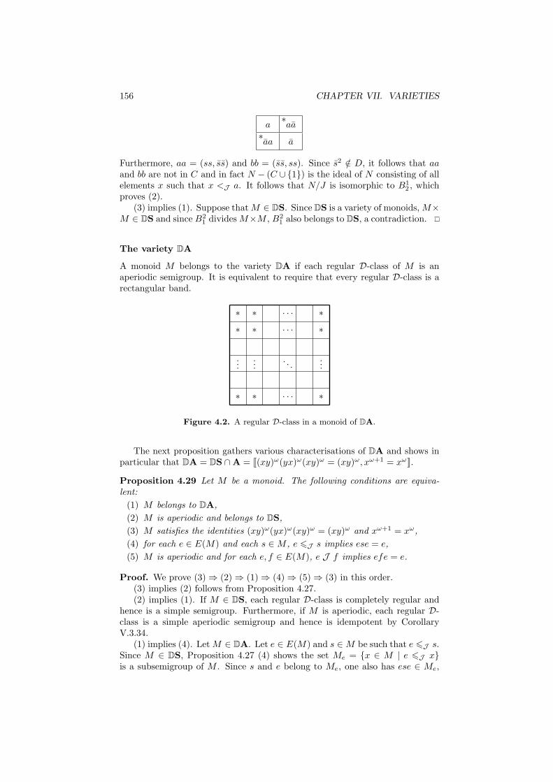
156 CHAPTER VII. VARIETIES
a∗aa
∗aa a
Furthermore, aa = (ss, ss) and bb = (ss, ss). Since s2 /∈ D, it follows that aaand bb are not in C and in fact N − (C ∪ {1}) is the ideal of N consisting of allelements x such that x <J a. It follows that N/J is isomorphic to B1
2 , whichproves (2).
(3) implies (1). Suppose thatM ∈ DS. Since DS is a variety of monoids,M×M ∈ DS and since B2
1 dividesM×M , B21 also belongs to DS, a contradiction.
The variety DA
A monoid M belongs to the variety DA if each regular D-class of M is anaperiodic semigroup. It is equivalent to require that every regular D-class is arectangular band.
∗
...
∗
∗
∗
...
∗
∗
. . .
. . .
. . .
. . .
∗
...
∗
∗
Figure 4.2. A regular D-class in a monoid of DA.
The next proposition gathers various characterisations of DA and shows inparticular that DA = DS ∩A = J(xy)ω(yx)ω(xy)ω = (xy)ω, xω+1 = xωK.
Proposition 4.29 Let M be a monoid. The following conditions are equiva-lent:
(1) M belongs to DA,
(2) M is aperiodic and belongs to DS,
(3) M satisfies the identities (xy)ω(yx)ω(xy)ω = (xy)ω and xω+1 = xω,
(4) for each e ∈ E(M) and each s ∈M , e 6J s implies ese = e,
(5) M is aperiodic and for each e, f ∈ E(M), e J f implies efe = e.
Proof. We prove (3)⇒ (2)⇒ (1)⇒ (4)⇒ (5)⇒ (3) in this order.(3) implies (2) follows from Proposition 4.27.(2) implies (1). If M ∈ DS, each regular D-class is completely regular and
hence is a simple semigroup. Furthermore, if M is aperiodic, each regular D-class is a simple aperiodic semigroup and hence is idempotent by CorollaryV.3.34.
(1) implies (4). LetM ∈ DA. Let e ∈ E(M) and s ∈M be such that e 6J s.Since M ∈ DS, Proposition 4.27 (4) shows the set Me = {x ∈ M | e 6J x}is a subsemigroup of M . Since s and e belong to Me, one also has ese ∈ Me,

4. EXAMPLES OF VARIETIES 157
and hence e 6J ese. Since ese 6J e one gets finally ese J e. But each regularD-class of M is a rectangular band, and thus ese = e.
(4) implies (5). For each x ∈ M , one has xω 6J x, and thus by (4),xω+1 = xω. ThereforeM is aperiodic. Moreover if e and f are two J -equivalentidempotents of M , then e 6J f and by (4), efe = e.
(5) implies (3). Suppose that M satisfies (5). Then M is aperiodic and sat-isfies the identity xω+1 = xω. Furthermore if x, y ∈M , the elements (xy)ω and(yx)ω are two conjugate idempotents, which are J -equivalent by PropositionV.2.22. It follows that (xy)ω(yx)ω(xy)ω = (xy)ω.
4.3 Varieties of ordered monoids
We denote by N+ [N−] the variety of ordered semigroups defined by the iden-tities yxω = xω = xωy and y 6 xω [yxω = xω = xωy and xω 6 y].
We let J+1[J−
1] denote the variety of ordered monoids defined by the identities
x2 = x, xy = yx and 1 6 x [x 6 1]. Proposition 4.24 can be readily adapted tothe ordered case.
Proposition 4.30 The variety J+1
[J−1] is generated by the monoid U+
1 [U−1 ].
We let J+ [J−] denote the variety of ordered monoids defined by the identityx 6 1 [1 6 x]. The notation is justified by the following result.
Proposition 4.31 An ordered monoid satisfying the identity 1 6 x [x 6 1] isJ -trivial.
Proof. Recall that the profinite word xω is defined as the limit of the sequencexn!. Similarly, the profinite word xω−1 is defined as the limit of the sequencexn!−1. It follows that (xy)ω = (xy)ω(xy)ω = (xy)ωx(yx)ω−1y.
Let M be an ordered monoid satisfying the identity 1 6 x. This identitygives 1 6 (yx)ω−1y and thus (xy)ω 6 (xy)ωx 6 (xy)ωx(yx)ω−1y 6 (xy)ω.Therefore, M satisfies the identities (xy)ωx = (xy)ω and, by a dual argument,y(xy)ω = (xy)ω. It follows by Proposition 4.23 that M is J -trivial.
A locally positive J -trivial semigroup is an ordered semigroup S such that,for each idempotent e ∈ S, the ordered semigroup eSe is positive J -trivial.Locally positive J -trivial semigroups form a variety of ordered semigroups, de-noted by LJ+ and defined by the identity Jxω 6 xωyxωK. This variety plays acrucial role in the study of the polynomial closure (see Chapter XII).
4.4 Summary
We summarise in the next table the varieties defined so far.

158 CHAPTER VII. VARIETIES
Notation Name Profinite identities
G Groups Jxω = 1K
Com Commutative monoids Jxy = yxK
J J -trivial monoids Jy(xy)ω = (xy)ω = (xy)ωxK
R R-trivial monoids J(xy)ωx = (xy)ωK
L L-trivial monoids Jy(xy)ω = (xy)ωK
J1 Semilattices Jx2 = x, xy = yxK
R1 Idempotent and R-trivial Jxyx = xyK
L1 Idempotent and L-trivial Jxyx = yxK
A Aperiodic monoids Jxω+1 = xωK
DARegular D-classes are J(xy)ω(yx)ω(xy)ω = (xy)ω,
aperiodic semigroups xω+1 = xωK
DSRegular D-classes
J((xy)ω(yx)ω(xy)ω)ω= (xy)ωK
are semigroups
Notation Name Profinite identities
N Nilpotent semigroups Jyxω = xω = xωyK
ℓ1 or K Lefty trivial semigroups Jxωy = xωK
r1 or D Righty trivial semigroups Jyxω = xωK
L1 Locally trivial semigroups Jxωyxω = xωK
LG Locally groups J(xωyxω)ω = xωK
CS Simple semigroups Jxω+1 = x, (xyx)ω = xωK
N+ Jyxω = xω = xωy, y 6 xωK
N− Jyxω = xω = xωy, xω 6 yK
J+1
Jx2 = x, xy = yx, 1 6 xK
J−1
Jx2 = x, xy = yx, x 6 1K
J+ J1 6 xK
J− Jx 6 1K
LJ+ Jxω 6 xωyxωK
5 Exercises
Section 1In Exercises 1 and 2, we exceptionally consider infinite monoids.
1. A Birkhoff variety of monoids is a class V of (possibly infinite) monoids suchthat:
(1) if S ∈ V and if T is a submonoid of S, then S ∈ V,
5. EXERCISES 159
(2) if S ∈ V and if T is a quotient of S, then S ∈ V,
(3) if (Si)i∈I is a (possibly infinite) family of monoids of V, the product∏i∈I Si is also in V.
Show that the class of all commutative monoids forms a Birkhoff variety, butthat the class of all groups does not (consider the submonoid N of Z).
2. Let A be an alphabet and let u, v ∈ A∗. A monoid M satisfies the identityu = v if and only if, for each monoid morphism ϕ : A∗ →M , ϕ(u) = ϕ(v).Show that a class of monoids is a Birkhoff variety if and only if it can bedefined by a set of identities (Birkhoff’s theorem). Birkhoff’s theorem can beextended to any variety of algebras, including semigroups, ordered semigroupsand ordered monoids.
Section 2We are now back with the usual convention of this chapter: semigroups areeither finite or free.
3. Let G denote the variety of finite groups and let dG be the function definedon page 142. Thus one has
rG(u, v) = min{Card(G) G is a finite group separating u and v }
and dG(u, v) = 2−rG(u,v) with the usual convention min ∅ = +∞ and 2−∞ = 0.
(1) Given two distinct words, prove that there exists a permutation automatonaccepting one of the words and rejecting the other one. Conclude that dGis a metric on A∗.
(2) We are interested now in the topology on A∗ defined by dG. Show thatfor each u ∈ A∗, one has limn→∞ un! = 1. Conclude that if L is a closedsubset of A∗, and if xu+y ⊆ L, the xu∗y ⊆ L.
(3) Show that the group languages of A∗ are clopen in the metric space(A∗, dG).
Section 3
4. Let GS be the variety of semigroups generated by all groups. Show thatGS = Jxωy = yxω = yK.
5. Show that the variety N is defined by the identity yxωz = xω. Show thatthe group Z/2Z satisfies the semigroup identity yxωy = xω. Conclude that thisidentity does not define N.
Section 4
6. Let V be a variety of [ordered] monoids. A semigroup S is locally V if,for every idempotent e of S, the [ordered] semigroup eSe belongs to V. Showthat the locally V [ordered] semigroups form a variety of [ordered] semigroups,denoted by LV.
7. Let V be the variety of monoids. Given a monoid M , let 〈E(M)〉 denote thesubmonoid of M generated by the idempotents of M . Show that the monoidsM such that 〈E(M)〉 belongs to V form a variety of monoids, denoted by EV.
160 CHAPTER VII. VARIETIES
8. Let V be the class of all finite monoidsM such that es = se for all e ∈ E(M)and all s ∈M .
(1) Show that V is a variety of finite monoids.
(2) Show that every monoid of V has a zero.
(3) Let M be a monoid of V and let e ∈ E(M). Show that the functionα :M → eM defined by α(s) = es is a monoid morphism.
(4) Let π be the projection from M onto M/MeM . Show that the functionγ : M → eM × (M/MeM) defined by γ(s) = (α(s), π(s)) is an injectivemorphism.
(5) Deduce that V is generated by the monoids of the form S1, where S is anilpotent semigroup.
6 Notes
Reference books on varieties include [3, 40, 91]. Varieties of ordered monoidswere first introduced in [94].

Chapter VIII
Equations and languages
In this chapter, we show how profinite words can be used to give algebraicdescriptions of certain classes of regular languages. Examples are deferred tothe next chapter.
1 Equations
Formally, a profinite equation is a pair (u, v) of profinite words of A∗. We alsouse the term explicit equation when both u and v are words of A∗. We saythat a recognisable language L of A∗ satisfies the profinite equation u → v (orv ← u) if the condition u ∈ L implies v ∈ L.
Proposition VI.3.13 gives immediately some equivalent definitions:
Corollary 1.1 Let L be a recognisable language of A∗, let η be its syntacticmorphism and let ϕ be any morphism onto a finite monoid recognising L. Thefollowing conditions are equivalent:
(1) L satisfies the equation u→ v,
(2) η(u) ∈ η(L) implies η(v) ∈ η(L),
(3) ϕ(u) ∈ ϕ(L) implies ϕ(v) ∈ ϕ(L).
The following result shows that equations behave very nicely with respectto complement.
Proposition 1.2 Let L be a recognisable language of A∗. Then L satisfies theequation u→ v if and only if Lc satisfies the equation v → u.
Proof. Let η be the syntactic morphism of L, which is also the syntactic mor-phism of Lc. By Corollary 1.1, L satisfies the equation u → v if and only if
η(u) ∈ η(L) implies η(v) ∈ η(L) (1.1)
Similarly, Lc satisfies the equation v → u if and only if η(v) ∈ η(Lc) impliesη(u) ∈ η(Lc). But since η(Lc) = η(L)c, the later implication can be written asη(v) /∈ η(L) implies η(u) /∈ η(L), which is the contrapositive of (1.1).
161

162 CHAPTER VIII. EQUATIONS AND LANGUAGES
2 Equational characterisation of lattices
Given a set E of equations of the form u→ v, the subset of Rec(A∗) defined byE is the set of all recognisable languages of A∗ satisfying all the equations of E.
A lattice of languages of A∗ is a set of recognisable languages of A∗ containingthe empty language ∅, the full language A∗ and which is closed under finite unionand finite intersection.
Proposition 2.3 The set of recognisable languages of A∗ defined by a set ofequations forms a lattice of languages.
Proof. Let E be a set of equations and let L be the class of languages of A∗
defined by E. We claim that L is a lattice. First, it is clear that the emptylanguage and the full language A∗ satisfy any equation of the form u → v.Therefore, these two languages are in L.
Let now L1 and L2 be languages of L and let u → v be an equation of E.Then, for i = 1, 2, the condition u ∈ Li implies v ∈ Li. Recall that, by TheoremVI.3.15, one has L1 ∪ L2 = L1 ∪ L2 and L1 ∩ L2 = L1 ∩ L2. Suppose thatu ∈ L1 ∪ L2. Then either u ∈ L1 or u ∈ L2 and thus either v ∈ L1 or v ∈ L2
and finally v ∈ L1 ∪ L2. Similarly, if u ∈ L1 ∩ L2, then u ∈ L1 and u ∈ L2,whence v ∈ L1 and v ∈ L2 and finally v ∈ L1 ∩ L2.
It follows that L1 ∩ L2 and L1 ∪ L2 satisfy all the equations of E and thusL is a lattice of languages.
Our aim is now to show that the converse of Proposition 2.3 also holds. Westart with a result on languages interesting on its own right. Note in particularthat there is no assumption on the languages in this proposition.
Proposition 2.4 Let L, L1, . . . , Ln be languages. If L satisfies all the explicitequations satisfied by L1, . . . , Ln, then L belongs to the lattice of languages gen-erated by L1, . . . , Ln.
Proof. We claim thatL =
⋃
I∈I
⋂
i∈I
Li (2.2)
where I is the set of all subsets I of {1, . . . , n} for which there exists a wordv ∈ L such that v ∈ Li if and only if i ∈ I.
Let R be the right-hand side of (2.2). If u ∈ L, let I = {i | u ∈ Li}. Byconstruction, I ∈ I and u ∈ ∩i∈ILi. Thus u ∈ R. This proves the inclusionL ⊆ R.
To prove the opposite direction, consider a word u ∈ R. By definition, thereexists a set I ∈ I such that u ∈ ∩i∈ILi and a word v ∈ L such that v ∈ Li
if and only if i ∈ I. We claim that the equation v → u is satisfied by eachlanguage Li. Indeed, if i ∈ I, then u ∈ Li by definition. If i /∈ I, then v /∈ Li
by definition of I, which proves the claim. It follows that v → u is also satisfiedby L. Since v ∈ L, it follows that u ∈ L. This concludes the proof of (2.2) andshows that L belongs to the lattice of languages generated by L1, . . . , Ln.
An important consequence of Proposition 2.4 is that finite lattices of lan-guages can be defined by explicit equations.

2. EQUATIONAL CHARACTERISATION OF LATTICES 163
Corollary 2.5 A finite set of languages of A∗ is a lattice of languages if andonly if it can be defined by a set of explicit equations of the form u→ v, whereu, v ∈ A∗.
Proof. Proposition 2.3 shows that a set of recognisable languages defined by aset of equations form a lattice of languages.
To prove the opposite direction, consider a finite lattice L of languages andlet E be the set of explicit equations satisfied by all the languages of L. Propo-sition 2.4 shows that any language L that satisfies the equations of E belongsto L. Thus L is defined by E.
We now are ready for the main result.
Theorem 2.6 A set of recognisable languages of A∗ is a lattice of languagesif and only if it can be defined by a set of equations of the form u → v, whereu, v ∈ A∗.
Proof. For each recognisable language L, set
EL = {(u, v) ∈ A∗ × A∗ | L satisfies u→ v}
Lemma 2.7 For each recognisable language L, EL is a clopen subset of A∗×A∗.
Proof. One has
EL = {(u, v) ∈ A∗ × A∗ | L satisfies u→ v}
= {(u, v) ∈ A∗ × A∗ | u ∈ L implies v ∈ L}
= {(u, v) ∈ A∗ × A∗ | v ∈ L or u /∈ L}
= (Lc× A∗) ∪ (A∗ × L)
The result follows since, by Proposition VI.3.12, L is clopen.
Let L be a lattice of languages and let E be the set of profinite equationssatisfied by all languages of L. We claim that E defines L. First, by definition,every language of L satisfies the equations of E. It just remains to prove thatif a language L satisfies the equations of E, then L belongs to L.
First observe that the set
{EL} ∪ {EcK | K ∈ L}
is a covering of A∗ × A∗. Indeed, if (u, v) /∈ ∪K∈LEcK , then (u, v) ∈ ∩K∈LEK ,
which means that u→ v is an equation satisfied by all languages of L. It followsthat L also satisfies this equation, and thus (u, v) ∈ EL. Furthermore, Lemma
2.7 shows that the elements of this covering are open sets. Since A∗ × A∗ iscompact, it admits a finite subcovering, and we may assume that this coveringcontains EL and is equal to
{EL} ∪ {EcL1, . . . , Ec
Ln}
for some languages L1, . . . , Ln of L. By the same argument as above, it followsthat if an equation u → v is satisfied by L1, . . . , Ln, then it is satisfied by L.

164 CHAPTER VIII. EQUATIONS AND LANGUAGES
By Proposition 2.4, L belongs to the lattice of languages generated by L1, . . . ,Ln and hence belongs to L.
Writing u ↔ v for (u → v and v → u), we get an equational description ofthe Boolean algebras of languages.
Corollary 2.8 A set of recognisable languages of A∗ is a Boolean algebra oflanguages if and only if it can be defined by a set of equations of the formu↔ v, where u, v ∈ A∗.
We now specialise Theorem 2.6 and Corollary 2.8 to interesting subcases.We consider lattices of languages closed under quotient in Section 3, streamsof languages in Section 4, C-streams in Section 5 and varieties of languages inSection 6.
3 Lattices of languages closed under quotients
We say that a class L of recognisable languages is a lattice of languages closedunder quotients if for every L ∈ L and u ∈ A∗, u−1L and Lu−1 are also in L.
Let u and v be two profinite words of A∗. We say that L satisfies theequation u 6 v if, for all x, y ∈ A∗, it satisfies the equation xuy → xvy. SinceA∗ is dense in A∗, it is equivalent to state that L satisfies these equations onlyfor all x, y ∈ A∗. But there is a much more convenient characterisation usingthe syntactic ordered monoid of L.
Proposition 3.9 Let L be a recognisable language of A∗, let (M,6L) be itssyntactic ordered monoid and let η : A∗ →M be its syntactic morphism. ThenL satisfies the equation u 6 v if and only if η(u) 6L η(v).
Proof. Corollary 1.1 shows that L satisfies the equation u 6 v if and only if,for every x, y ∈ A∗, η(xvy) ∈ η(L) implies η(xvy) ∈ η(L). Since η(xuy) =η(x)η(u)η(y) = η(x)η(u)η(y) and since η is surjective, this is equivalent tosaying that, for all s, t ∈M , sη(u)t ∈ η(L) implies sη(v)t ∈ η(L), which exactlymeans that η(u) 6L η(v).
We can now state the equational characterisation of lattices of languagesclosed under quotients.
Theorem 3.10 A set of recognisable languages of A∗ is a lattice of languagesclosed under quotients if and only if it can be defined by a set of equations ofthe form u 6 v, where u, v ∈ A∗.
Proof. Let L be a recognisable language satisfying the equation u 6 v and letx, y ∈ A∗. Since L satisfies the equation xuy → xvy, the condition xuy ∈ L im-plies xvy ∈ L and hence u ∈ x−1Ly−1 implies v ∈ x−1Ly−1. Since x−1Ly−1 =x−1Ly−1 by Proposition VI.3.16, the language x−1Ly−1 satisfies the equationu 6 v. It follows that the set of recognisable languages defined by a set ofequations of the form u 6 v is a lattice of languages closed under quotients.
In the opposite direction, let L be a lattice of languages of A∗ closed underquotients. By Theorem 2.6, L can be defined by a set E of equations of the formu → v, where u, v ∈ A∗. Let now u → v be an equation of E, L a language of

4. STREAMS OF LANGUAGES 165
L and x, y two words of A∗. Since L is closed under quotient, x−1Ly−1 belongsto L and thus satisfies also the equation u → v. It follows that L satisfies theequation xuy → xvy and hence L satisfies the equation u 6 v. It follows that Lis defined by the equations of the form u 6 v where u→ v is an equation of E.
Theorem 3.10 can be readily extended to Boolean algebras. Let u and v betwo profinite words. We say that a recognisable language L satisfies the equationu = v if it satisfies the equations u 6 v and v 6 u. Proposition 3.9 now givesimmediately:
Proposition 3.11 Let L be a recognisable language of A∗ and let η be its syn-tactic morphism. Then L satisfies the equation u = v if and only if η(u) = η(v).
This leads to the following equational description of Boolean algebras oflanguages closed under quotients.
Corollary 3.12 A set of recognisable languages of A∗ is a Boolean algebra oflanguages closed under quotients if and only if it can be defined by a set ofequations of the form u = v, where u, v ∈ A∗.
4 Streams of languages
A class of recognisable languages is a correspondence F which associates witheach alphabet A a set F(A∗) of recognisable languages of A∗ in such a way that,if σ : A → B is a bijection, a language L belongs to F(A∗) if and only if σ(L)belongs to F(B∗). It follows that, if we fix for each nonnegative integer n analphabet An = {a1, . . . , an}, the class F is completely determined by the family(F(A∗
n))n∈N.We use here the terms class and correspondence instead of set and function
to avoid any paradox of set theory, since it is known, for instance, that the finitesets do not form a set. However, we shall use the term “bijection” instead of“one-to-one and onto correspondence”.
A positive stream of languages is a class of recognisable languages V such that
(1) for each alphabet A, V(A∗) is a lattice of languages,
(2) for each monoid morphism ϕ : A∗ → B∗, X ∈ V(B∗) implies ϕ−1(X) ∈V(A∗),
A stream of languages is a positive stream of languages closed under comple-mentation. This amounts to replacing (1) by (1’) in the previous definition
(1′) for each alphabet A, V(A∗) is a Boolean algebra.
In the sequel, we fix for each nonnegative integer n an alphabet An ={a1, . . . , an}. Let u and v be two profinite words of A∗
n and let L be a recog-nisable language of A∗. One says that L satisfies the profinite identity u → v[u↔ v] if, for each morphism γ : A∗
n → A∗, L satisfies the equation γ(u)→ γ(v)[γ(u)↔ γ(v)]. The next proposition gives an alternative definition.
Proposition 4.13 Let L be a recognisable language of A∗ and let ϕ : A∗ →Mbe any surjective morphism onto a finite monoid recognising L. Then L satisfiesthe profinite identity u→ v, where u, v ∈ A∗
n, if and only if, for every morphismα : A∗
n →M , α(u) ∈ ϕ(L) implies α(v) ∈ ϕ(L).

166 CHAPTER VIII. EQUATIONS AND LANGUAGES
Proof. Suppose that, for every morphism α : A∗n → M , α(u) ∈ ϕ(L) implies
α(v) ∈ ϕ(L). If γ : A∗n → A∗ is a morphism, then ϕ(γ(u)) ∈ ϕ(L) implies
ϕ(γ(v)) ∈ ϕ(L) and thus L satisfies the equation γ(u)→ γ(v).
In the opposite direction, suppose that L satisfies the profinite identity u→ vand let α : A∗
n →M be a morphism. By Corollary II.5.30, there is a morphismγ : A∗
n → A∗ such that ϕ◦γ = α. Now L satisfies the equation γ(u)→ γ(v) andthus, by Corollary 1.1, ϕ(γ(u)) ∈ ϕ(L) implies ϕ(γ(v)) ∈ ϕ(L). Since ϕ◦ γ = α,one gets α(u) ∈ ϕ(L) implies α(v) ∈ ϕ(L).
Theorem 4.14 A class of recognisable languages of A∗ is a positive stream oflanguages if and only if it can be defined by a set of profinite identities of theform u→ v. It is a stream of languages if and only if it can be defined by a setof profinite identities of the form u↔ v.
Before proving this theorem, let us clarify one point: the identities defininga stream are not necessarily on the same alphabet.
Proof. Let V be a class of languages defined by a set E of profinite identitiesof the form u → v. For each n, let En be the set of all identities u → v ofE such that u, v ∈ A∗
n. By definition, V(A∗) is the set of languages satisfyingall the equations of the form γ(u) → γ(v), where (u, v) ∈ En for some n andγ : A∗
n → A∗ is a morphism. In particular, Theorem 3.10 shows that V(A∗) is alattice of languages.
To prove that V is a positive stream of languages, it remains to prove thatit is closed under inverses of morphisms. Let ϕ : A∗ → B∗ be a morphism andlet L ∈ V(B∗). We claim that ϕ−1(L) satisfies all the identities of E. Indeed,let (u, v) ∈ En and let γ : A∗
n → B∗ be a morphism. We want to show thatϕ−1(L) satisfies the equation γ(u)→ γ(v). Suppose that γ(u) ∈ ϕ−1(L). SinceProposition VI.3.17 states that ϕ−1(L) = ϕ−1(L), one gets ϕ(γ(u)) ∈ L. Sinceϕ ◦ γ = ϕ ◦ γ, we finally get ϕ ◦ γ(u) ∈ L. Now, as L satisfies the identityu→ v, one obtains ϕ ◦ γ(v) ∈ L, which, by the same argument in reverse order,implies that γ(v) ∈ ϕ−1(L). This proves that ϕ−1(L) satisfies the equationγ(u) → γ(v) and thereby the identity u → v. This validates the claim andconfirms that ϕ−1(L) belongs to V(A∗). Therefore V is a positive stream oflanguages.
Let now V be a positive stream of languages. Then, for each n, the set V(A∗n)
is a lattice of languages and by Theorem 2.6, it is defined by a set En of profiniteequations of the form u→ v, with u, v ∈ A∗
n. We claim that these equations areactually identities satisfied by V. Let γ : A∗
n → A∗ be a morphism and let u→ vbe an equation of En. If L ∈ V(A∗), then γ−1(L) ∈ V(A∗
n) and thus γ−1(L)satisfies the equation u → v. Thus u ∈ γ−1(L) implies v ∈ γ−1(L). Now,Proposition VI.3.17 shows that γ−1(L) = γ−1(L) and thereby, the conditionsx ∈ γ−1(L) and γ(x) ∈ L are equivalent. Thus γ(u) ∈ L implies γ(v) ∈ L,which means that L satisfies the equation γ(u) → γ(v). Therefore u → v isan identity of V. It follows that V is defined by a set of identities of the formu→ v.

5. C-STREAMS 167
5 C-streams
Let C be a class of morphisms between finitely generated free monoids thatsatisfies the following properties :
(1) C is closed under composition. That is, if A, B and C are finite alphabets,and f : A∗ → B∗ and g : B∗ → C∗ are elements of C, then g ◦ f belongsto C.
(2) C contains all length-preserving morphisms.
Examples include the classes of all length-preserving morphisms (morphisms forwhich the image of each letter is a letter), of all length-multiplying morphisms(morphisms such that, for some integer k, the length of the image of a word is ktimes the length of the word), all non-erasing morphisms (morphisms for whichthe image of each letter is a nonempty word), all length-decreasing morphisms(morphisms for which the image of each letter is either a letter of the emptyword) and all morphisms.
A positive C-stream of languages is a class of recognisable languages V suchthat :
(1) for every alphabet A, V(A∗) is a lattice of languages,
(2) if ϕ : A∗ → B∗ is a morphism of C, L ∈ V(B∗) implies ϕ−1(L) ∈ V(A∗),
A C-stream of languages is a positive C-stream of languages closed under com-plement.
Let u and v be two profinite words of A∗n and let L be a recognisable language
of A∗. One says that L satisfies the profinite C-identity u→ v [u↔ v] if, for eachC-morphism γ : A∗
n → A∗, L satisfies the equation γ(u)→ γ(v) [γ(u)↔ γ(v)].
Theorem 5.15 A class of recognisable languages of A∗ is a positive C-streamof languages if and only if it can be defined by a set of profinite C-identities ofthe form u→ v. It is a stream of languages if and only if it can be defined by aset of profinite C-identities of the form u↔ v.
Proof. The proof of Theorem 4.14 carries over by changing every occurrenceof “morphism” by “C-morphism”. Note however that the closure of C undercomposition is needed to show that γ ◦ ϕ belongs to C.
The notion of C-identity can be sometimes confusing. Let us illustrate it bya few examples.
Example 5.1 A recognisable language L satisfies the identity [length-preserving,non-erasing, length-multiplying identity] xyx 6 yxy if, for all words [letters,nonempty words, words of the same length] x and y, the relation xyx 6L yxyholds.
6 Varieties of languages
A positive variety of languages is a class of recognisable languages such that
(1) for each alphabet A, V(A∗) is a lattice of languages,
(2) for each monoid morphism ϕ : A∗ → B∗, X ∈ V(B∗) implies ϕ−1(X) ∈V(A∗),
(3) If X ∈ V(A∗) and u ∈ A∗, u−1X ∈ V(A∗) and Xu−1 ∈ V(A∗).
168 CHAPTER VIII. EQUATIONS AND LANGUAGES
A variety of languages is a positive variety of languages closed under comple-mentation. This amounts to replacing (1) by (1′) in the previous definition
(1′) for each alphabet A, V(A∗) is a Boolean algebra.
Let u and v be two profinite words of A∗n and let L be a recognisable language
of A∗. One says that L satisfies the profinite identity u 6 v [u = v] if, for allmorphisms γ : A∗
n → A∗, L satisfies the equation γ(u) 6 γ(v) [γ(u) = γ(v)].
Theorem 6.16 A class of recognisable languages of A∗ is a positive variety oflanguages if and only if it can be defined by a set of profinite identities of theform u 6 v. It is a variety of languages if and only if it can be defined by a setof profinite identities of the form u = v.
Proof. The proof, which combines the arguments of Theorems 3.10 and 4.14 isleft as an exercise to the reader.
A positive C-variety of languages is a class of recognisable languages V such that
(1) for every alphabet A, V(A∗) is a lattice of languages,
(2) if ϕ : A∗ → B∗ is a morphism of C, L ∈ V(B∗) implies ϕ−1(L) ∈ V(A∗),
(3) if L ∈ V(A∗) and if a ∈ A, then a−1L and La−1 are in V(A∗).
A C-variety of languages is a positive C-variety of languages closed under com-plement.
Let u and v be two profinite words of A∗n and let L be a recognisable language
of A∗. One says that L satisfies the profinite C-identity u 6 v [u = v] if, for allC-morphisms γ : A∗
n → A∗, L satisfies the equation γ(u) 6 γ(v) [γ(u) = γ(v)].
Theorem 6.17 A class of recognisable languages of A∗ is a positive C-varietyof languages if and only if it can be defined by a set of profinite identities of theform u 6 v. It is a C-variety of languages if and only if it can be defined by aset of profinite identities of the form u = v.
Proof. The proof, which combines the arguments of Theorems 3.10 and 5.15 isleft as an exercise to the reader.
When C is the class of all morphisms, we recover the definition of a varietyof languages. When C is the class of length-preserving [length-multiplying, non-erasing, length-decreasing] morphisms, we use the term lp-variety [lm-variety,ne-variety, ld-variety] of languages.
7 The variety theorem
In this section, we present a slightly different algebraic point of view to charac-terise varieties of languages, proposed by Eilenberg [40].
If V is a variety of finite monoids, let V(A∗) denote the set of recognisablelanguages of A∗ whose syntactic monoid belongs to V. The following is anequivalent definition:
Proposition 7.18 V(A∗) is the set of languages of A∗ recognised by a monoidof V.

7. THE VARIETY THEOREM 169
Proof. If L ∈ V(A∗), then the syntactic monoid of L, which recognises L,belongs to V. Conversely, if L is recognised by a monoid M of V, then byProposition IV.4.25, the syntactic monoid of L divides M and thus belongs alsoto V.
The correspondence V → V associates with each variety of finite monoids aclass of recognisable languages. We shall see later (Proposition 7.21) that V is avariety of languages. For now, we show that this correspondence is one-to-one.
Theorem 7.19 Let V and W be two varieties of finite monoids. Suppose thatV→ V and W→W. Then V ⊆W if and only if, for every finite alphabet A,V(A∗) ⊆ W(A∗). In particular, V = W if and only if V =W.
Proof. If V ⊆ W, it follows immediately from the definitions that V(A∗) ⊆W(A∗). The proof of the opposite direction of the theorem is based on thefollowing proposition.
Proposition 7.20 Let V be a variety of monoids and let M ∈ V. Then thereexist a finite alphabet A and languages L1, . . . , Lk ∈ V(A∗) such that M isisomorphic to a submonoid of M(L1)× · · · ×M(Lk).
Proof. SinceM is finite, there exists a finite alphabet A and a surjective monoidmorphism ϕ : A∗ → M . For each s ∈ M , put Ls = ϕ−1(s). Then Ls isrecognised by M and thus Ls ∈ V(A
∗). Let Ms be the syntactic monoid of Ls.By Proposition IV.4.24, it is also the syntactic monoid of the singleton {s} inM . We let πs : M → Ms denote the projection and by π : M →
∏s∈M Ms
the morphism of monoids defined by π(x) = (πs(x))s∈M . We claim that π isinjective. If π(x) = π(y), then in particular, πy(x) = πy(y). This means that,for every s, t ∈ M , syt = y if and only if sxt = y. Applying this result withs = t = 1, one gets x = y. This proves the claim and shows thatM is isomorphicto a submonoid of
∏s∈M Ms.
We can now complete the proof of Theorem 7.19. Suppose that V(A∗) ⊆W(A∗) for every finite alphabet A and let M ∈ V. Then by Proposition7.20, M is isomorphic to a submonoid of the form M(L1) × · · · × M(Lk),where L1, . . . , Lk ∈ V(A
∗). It follows that L1, . . . , Lk ∈ W(A∗) and henceM(L1), . . . ,M(Lk) ∈W. Therefore M ∈W.
We now characterise the classes of languages which can be associated witha variety of monoids.
Proposition 7.21 Let V be a variety of finite monoids. If V → V, then V isa variety of languages.
Proof. Let L,L1, L2 ∈ V(A∗) and let a ∈ A. Then by definitionM(L), M(L1),M(L2) are in V. By Proposition IV.2.9, the languages L1 ∪L2 and L1 ∩L2 arerecognised by a submonoid T of M(L1) ×M(L2). Now since V is a variety ofmonoids, T ∈ V and thus L1∪L2 and L1∩L2 belong to V(A∗). Since ∅ and A∗
are recognised by the trivial monoid, which is certainly in V, V(A∗) is a Booleanalgebra of languages. Similarly, Proposition IV.2.11 shows that the languagesa−1L and La−1 are recognised by M(L) and Proposition IV.2.10 shows that, if
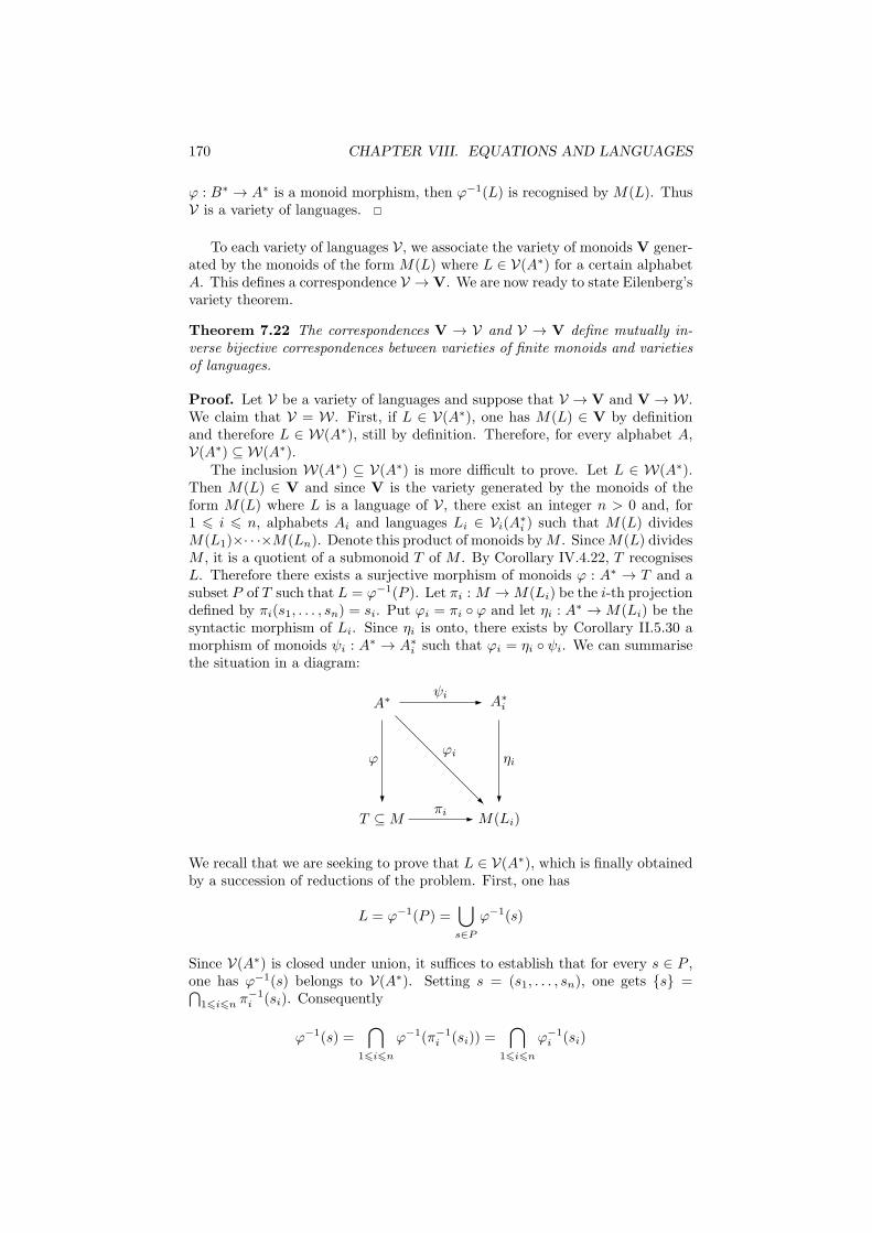
170 CHAPTER VIII. EQUATIONS AND LANGUAGES
ϕ : B∗ → A∗ is a monoid morphism, then ϕ−1(L) is recognised by M(L). ThusV is a variety of languages.
To each variety of languages V, we associate the variety of monoids V gener-ated by the monoids of the form M(L) where L ∈ V(A∗) for a certain alphabetA. This defines a correspondence V → V. We are now ready to state Eilenberg’svariety theorem.
Theorem 7.22 The correspondences V → V and V → V define mutually in-verse bijective correspondences between varieties of finite monoids and varietiesof languages.
Proof. Let V be a variety of languages and suppose that V → V and V→W.We claim that V = W. First, if L ∈ V(A∗), one has M(L) ∈ V by definitionand therefore L ∈ W(A∗), still by definition. Therefore, for every alphabet A,V(A∗) ⊆ W(A∗).
The inclusion W(A∗) ⊆ V(A∗) is more difficult to prove. Let L ∈ W(A∗).Then M(L) ∈ V and since V is the variety generated by the monoids of theform M(L) where L is a language of V, there exist an integer n > 0 and, for1 6 i 6 n, alphabets Ai and languages Li ∈ Vi(A∗
i ) such that M(L) dividesM(L1)×· · ·×M(Ln). Denote this product of monoids byM . SinceM(L) dividesM , it is a quotient of a submonoid T of M . By Corollary IV.4.22, T recognisesL. Therefore there exists a surjective morphism of monoids ϕ : A∗ → T and asubset P of T such that L = ϕ−1(P ). Let πi :M →M(Li) be the i-th projectiondefined by πi(s1, . . . , sn) = si. Put ϕi = πi ◦ ϕ and let ηi : A
∗ →M(Li) be thesyntactic morphism of Li. Since ηi is onto, there exists by Corollary II.5.30 amorphism of monoids ψi : A
∗ → A∗i such that ϕi = ηi ◦ ψi. We can summarise
the situation in a diagram:
A∗ A∗i
T ⊆M M(Li)
ψi
πi
ηiϕiϕ
We recall that we are seeking to prove that L ∈ V(A∗), which is finally obtainedby a succession of reductions of the problem. First, one has
L = ϕ−1(P ) =⋃
s∈P
ϕ−1(s)
Since V(A∗) is closed under union, it suffices to establish that for every s ∈ P ,one has ϕ−1(s) belongs to V(A∗). Setting s = (s1, . . . , sn), one gets {s} =⋂
16i6n π−1i (si). Consequently
ϕ−1(s) =⋂
16i6n
ϕ−1(π−1i (si)) =
⋂
16i6n
ϕ−1i (si)
7. THE VARIETY THEOREM 171
As V(A∗) is a lattice, it suffices to establish that, for 1 6 i 6 n, ϕ−1i (si) ∈ V(A∗).
Since ϕi = ηi ◦ψi, one has ϕ−1i (si) = ψ−1
i (η−1i (si)). Now since V is a variety
of languages, it suffices to prove that η−1i (si) ∈ V(A∗
i ), which results from thefollowing lemma.
Lemma 7.23 Let V be a variety of languages and let η : A∗ → M be thesyntactic morphism of a language L of V(A∗). Then for every x ∈ M , η−1(x)belongs to V(A∗).
Proof. Let P = η(L). Then L = η−1(P ). Setting E = {(s, t) ∈M2 | sxt ∈ P},we claim that
{x} =( ⋂
(s,t)∈E
s−1Pt−1)−( ⋃
(s,t)∈Ec
s−1Pt−1)
(7.3)
Let R be the right-hand side of (7.3). It is clear that x belongs to R. Conversely,let u be an element of R. If sxt ∈ P , then u ∈ s−1Pt−1, that is, sut ∈ P . And ifsxt /∈ P , then u /∈ s−1Pt−1. It follows that u ∼L x and thus u = x, which provesthe claim. Since η−1 commutes with Boolean operations and quotients, η−1(x)is a Boolean combination of quotients of L and hence belongs to V(A∗).
There is an analoguous theorem for varieties of ordered monoids.
Theorem 7.24 The correspondences V → V and V → V define mutually in-verse bijective correspondences between varieties of finite ordered monoids andpositive varieties of languages.
Eilenberg’s +-varieties
In his original presentation, Eilenberg introduced a variant of his variety the-orem. We shall briefly review this version and discuss its connexion with thepoint of view presented in this chapter.
The first difference is that languages are now subsets of a free semigroup,instead of a free monoid in the usual case. In this setting, it is natural to usesemigroups instead of monoids and in particular, there is a notion of syntacticsemigroup. A +-variety of languages is a class of recognisable languages suchthat
(1) for each alphabet A, V(A+) is a Boolean algebra,
(2) for each semigroup morphism ϕ : A+ → B+, ifX ∈ V(B+) then ϕ−1(X) ∈V(A+),
(3) If X ∈ V(A+) and u ∈ A∗, u−1X ∈ V(A+) and Xu−1 ∈ V(A+).
Positive +-varieties of languages can be defined in the same way. The secondEilenberg’s
Theorem 7.25 The correspondences V → V and V → V define mutually in-verse bijective correspondences between varieties of finite semigroups and +-varieties of languages.
There is an analoguous theorem for varieties of ordered semigroups.
172 CHAPTER VIII. EQUATIONS AND LANGUAGES
Theorem 7.26 The correspondences V → V and V → V define mutually in-verse bijective correspondences between varieties of finite ordered semigroupsand positive +-varieties of languages.
To interpret this result in the context of this chapter, let us introduce anotation: if S is a semigroup, let SI denote the monoid S ∪ {I}, where I is anew identity.
LetV be a variety of finite semigroups and let V be the corresponding varietyof languages. We define another class of languages V ′ as follows. For eachalphabet A, V ′(A∗) consists of all languages of A∗ recognised by a morphismϕ : A∗ → SI such that the semigroup ϕ(A+) is in V. This is the case inparticular if S ∈ V and ϕ : A+ → S is a surjective morphism. Then one canshow that V is a ne-variety of languages. Moreover, every language of V(A+) isa language of V ′(A∗). Conversely, if L is a language of V ′(A∗), then L ∩ A+ isa language of V(A+).
8 Summary
We summarise in a table the various types of equations we have used so far.
Closed under Equations Definition
∪,∩ u→ v η(u) ∈ η(L)⇒ η(v) ∈ η(L)
quotient u 6 v xuy → xvy
complement u↔ v u→ v and v → u
quotient and complement u = v xuy ↔ xvy
Closed under inverses of morphisms Interpretation of variables
all morphisms words
nonerasing morphisms nonempty words
length multiplying morphisms words of equal length
length preserving morphisms letters
9 Exercises
1. Let A = {a, b} and L = (a2)∗b(a2)∗b. Compute the syntactic monoidM of L(you should find 12 elements and 6 J -classes). Does L satisfy the the followingprofinite equations:
(1) (xy)ω = (yx)ω for all x, y ∈ A∗,
(2) xωyxω = xωyxωyxω for all x, y ∈ A+,
(3) xωyω = yωxω for all x, y ∈ A∗.
10 Notes
The results presented in Sections 1, 2 and 3 were first presented in [45]. Varietiesof languages and the variety theorem (Section 7) are due to Eilenberg [40]. C-
10. NOTES 173
varieties were introduced by Straubing [153] and under a slightly different form,by Esik [42].
174 CHAPTER VIII. EQUATIONS AND LANGUAGES
Chapter IX
Algebraic characterisations
In this chapter, we give explicit examples of the algebraic characterisationsdescribed in Chapter VI.
1 Varieties of languages
The two simplest examples of varieties of languages are the variety I corre-sponding to the trivial variety of monoids 1 and the variety Rat of rationallanguages corresponding to the variety of all monoids. For each alphabet A,I(A∗) consists of the empty and the full language A∗ and Rat(A∗) is the set ofall rational languages on the alphabet A.
We provide the reader with many more examples in this section. Otherimportant examples are the topic of Chapters X, XI and XIV.
1.1 Locally finite varieties of languages
Let V be a [positive] variety of languages. One says that V is locally finite ifthe corresponding variety of [ordered] monoids is locally finite. Here is a morecombinatorial characterisation.
Proposition 1.1 A [positive] variety of languages V is locally finite if and onlyif, for each alphabet A, V(A∗) is a finite set.
Proof. Let V be the variety of [ordered] monoids corresponding to V. If V
is locally finite, then, for each alphabet A, FV(A) is a finite monoid whichrecognises all the languages of V(A∗). It follows that V(A∗) is a finite set.
Conversely, suppose that for each alphabet A, V(A∗) is a finite set. Define anequivalence ≡V on A∗ by u ≡V v if and only if, for all L ∈ V(A∗), the conditionsu ∈ L and v ∈ L are equivalent. Since V(A∗) is finite, this equivalence has finiteindex. We claim that u ≡V v implies u ∼V v. Indeed, let ϕ be a morphismfrom A∗ onto a monoid M of V and suppose that u ≡V v. Then the languageL = ϕ−1(ϕ(u)) belongs to V(A∗) and since u ∈ L, one gets v ∈ L, that isϕ(v) = ϕ(u), which proves the claim. It follows that ∼V has finite index and
thus FV(A) is a finite monoid.
175

176 CHAPTER IX. ALGEBRAIC CHARACTERISATIONS
A combinatorial description
Proposition VII.2.8 shows that if V is generated by a single [ordered] monoid,then V is locally finite. In this case, one can give a more precise description ofV.
Proposition 1.2 Let V be a variety of ordered monoids generated by a singleordered monoid M and let V be the corresponding positive variety. Then, foreach alphabet A, V(A∗) is the lattice generated by the sets of the form ϕ−1(↑m),where ϕ : A∗ →M is an arbitrary morphism and m ∈M .
Proof. It is clear that ϕ−1(↑ m) ∈ V(A∗) and thus V(A∗) also contains thelattice generated by these sets. Conversely, let L ∈ V(A∗). Then there existsan integer n > 0, a morphism ϕ : A∗ →Mn and an upper set I of M such thatL = ϕ−1(I). Since ϕ−1(I) =
⋃m∈P ϕ
−1(↑m), it is sufficient to establish theresult when L = ϕ−1(↑m) where m ∈ Mn. Denote by πi the i-th projectionfrom Mn onto M . Setting m = (m1, . . . ,mn), we have m =
⋂16i6n π
−1i (mi),
whence
ϕ−1(↑m) =⋂
16i6n
(πi ◦ ϕ)−1(↑mi)
Since mi ∈M and πi ◦ ϕ is a morphism from A∗ into M , the result follows.
There is of course a similar result for the varieties of monoids, the proof ofwhich is similar.
Proposition 1.3 Let V be a variety of monoids generated by a single monoidM and let V be the corresponding variety of languages. Then, for every alphabetA, V(A∗) is the Boolean algebra generated by the sets of the form ϕ−1(m), whereϕ : A∗ →M is an arbitrary morphism and m ∈M .
Languages corresponding to J1, J+1
and J−1
Let J1 [J +1 , J−
1 ] denote the [positive] variety of languages corresponding to J1
[J+1, J−
1].
Proposition 1.4 For each alphabet A, J1(A∗) is the Boolean algebra generated
by the languages of the form A∗aA∗ where a is a letter. Equivalently, J1(A∗)
is the Boolean algebra generated by the languages of the form B∗ where B is asubset of A.
Proof. The equality of the two Boolean algebras considered in the statementresults from the formulas
B∗ = A∗ −⋃
a∈A−B
A∗aA∗ and A∗aA∗ = A∗ − (A− {a})∗
Since J1 is generated by U1, one can use Proposition 1.3 to describe J1. Let ϕ :A∗ → U1 be a morphism, and let B = {a ∈ A | ϕ(a) = 1}. Then ϕ−1(1) = B∗
and ϕ−1(0) = A∗ −B∗, which establishes the proposition.

1. VARIETIES OF LANGUAGES 177
If B is a subset of A, let F (B) denote the set of words of A∗ containing atleast one occurrence of each letter of B. Thus
F (B) =⋂
a∈B
A∗aA∗
The next proposition is thus a variant of Proposition 1.4 and its proof is left asan exercise to the reader.
Proposition 1.5 For each alphabet A, J +1 (A∗) is the set of finite unions of
languages of the form F (B) where B ⊆ A. Similarly, J−1 (A∗) is the set of
finite unions of languages of the form B∗ where B ⊆ A.
Languages corresponding to R1 and L1
Another interesting example of a locally finite variety is the variety R1 of idem-potent and R-trivial monoids.
Proposition 1.6 Let L be a recognisable subset of A∗ and letM be its syntacticmonoid. The following conditions are equivalent:
(1) M divides Un2 for some n > 0,
(2) M belongs to R1,
(3) M satisfies the identity xyx = xy,
(4) L is a disjoint union of sets of the form
a1{a1}∗a2{a1, a2}
∗a3{a1, a2, a3}∗ · · · an{a1, a2, . . . , an}
∗
where the ai’s are distinct letters of A,
(5) L is a Boolean combination of sets of the form B∗aA∗, where a ∈ A andB ⊆ A.
Proof. (1) implies (2) since U2 ∈ R1.(2) implies (3). Let x, y ∈ M . Since M is idempotent, xy = xyxy and thusxy R xyx. But M is R-trivial and therefore xy = xyx.(3) implies (4). Let ρ : A∗ → A∗ be the function which associates with any wordu the sequence of all distinct letters of u in the order in which they first appearwhen u is read from left to right. For example, if u = caabacb, then ρ(u) = cab.In fact ρ is a sequential function, realised by the sequential transducer T =(P(A), A, ∅, · , ∗), where the transition and the output functions are defined by
B · a = B ∪ {a}
B ∗ a =
{1 if a ∈ B
0 otherwise
Define an equivalence ∼ on A∗ by setting u ∼ v if ρ(u) = ρ(v). It is easy to seethat the equivalence classes of ∼ are the disjoint sets
L(a1,...,an) = a1{a1}∗a2{a1, a2}
∗a3{a1, a2, a3}∗ · · · an{a1, a2, . . . , an}
∗
where (a1, . . . , an) is a sequence of distinct letters of A. We claim that ∼ isa congruence. If u ∼ v, then u and v belong to some set L(a1,...,an). Let

178 CHAPTER IX. ALGEBRAIC CHARACTERISATIONS
a be a letter. If a = ai for some i, then ua, va ∈ L(a1,...,an), and au, av ∈L(a,a1,...,ai−1,ai+1,...,an). Thus ua ∼ va and au ∼ av. If a /∈ {a1, . . . , an}, thenua, va ∈ L(a1,...,an,a) and au, av ∈ L(a,a1,...,an) and thus again ua ∼ va andau ∼ av, which proves the claim.
Let η : A∗ → M be the syntactic morphism of L. If u ∈ L(a1,...,an), thenu = a1u1a2u2 · · · anun where ui ∈ {a1, . . . , ai}
∗ for 1 6 i 6 n and thus by (3),η(u) = η(a1 · · · an). It follows that u ∼ v implies η(u) = η(v) and therefore L isa disjoint union of equivalence classes of ∼, that is of sets of the form L(a1,...,an).(4) implies (5). First observe that
L(a1,...,an) = A∗n ∩
⋂
16i6n
A∗i−1aiA
∗ where Ai = {a1, . . . , ai} and A0 = ∅
Condition (5) is now a consequence of the following equalities:
A∗i = A∗ −
⋃
a/∈Ai
A∗aA∗ A∗i−1aiA
∗i = A∗
i−1aiA∗ ∩A∗
i
(5) implies (1). By the variety theorem (Theorem VIII.7.19), it is sufficientto show that, for B ⊆ A and a ∈ A, B∗aA∗ is recognised by U2. Let U2 ={1, a1, a2} and let ϕ : A∗ → U2 be the morphism defined by
ϕ(a) = a1
ϕ(b) =
{1 if b ∈ B − {a}
a2 for b ∈ A− (B ∪ {a})
Then ϕ−1(a1) = B∗aA∗, which concludes the proof.
There is of course a dual version for the variety L1 of idempotent and L-trivial monoids.
Proposition 1.7 Let L be a recognisable subset of A∗ and letM be its syntacticmonoid. The following conditions are equivalent:
(1) M divides Un2 for some n > 0,
(2) M belongs to L1,
(3) M satisfies the identity xyx = yx,
(4) L is a disjoint union of sets of the form
{a1, a2, . . . , an}∗an{a1, a2, . . . , an−1} · · · {a1, a2}
∗a2{a1}∗a1
where the ai’s are distinct letters of A,
(5) L is a Boolean combination of sets of the form A∗aB∗, where a ∈ A andB ⊆ A.
1.2 Commutative languages
We now come to the study of commutative languages. We study successivelythe languages corresponding to aperiodic and commutative monoids (varietyAcom), to commutative groups and to arbitrary commutative monoids.
1. VARIETIES OF LANGUAGES 179
Languages recognised by aperiodic commutative monoids
If a is a letter of an alphabet A, let L(a, k) denote the set of words of A∗ whichcontain exactly k occurrences of a
L(a, k) = {u ∈ A+ | |u|a = k}
Then the following result holds.
Proposition 1.8 For each alphabet A, Acom(A∗) is the Boolean algebra gen-erated by the sets of the form L(a, k) where a ∈ A and k > 0.
Proof. First, every set of the form L(a, k) is recognised by an aperiodic com-mutative monoid. Indeed, let N = {1, x, x2, . . . , xk, xk+1} be the cyclic monoiddefined by the relation xk+2 = xk+1, and let ϕ : A∗ → N be the morphismdefined by ϕ(a) = x and ϕ(b) = 1 if b 6= a. Then clearly L(a, k) = ϕ−1(xk).
By Proposition VII.4.21, Acom is generated by its cyclic monoids, andProposition 1.3 can be used to describe Acom. Let M = {1, x, x2, . . . , xn} bea cyclic monoid, defined by the relation xn+1 = xn, and let ϕ : A∗ → M be amorphism. Then for each a ∈ A there exists an integer na such that ϕ(a) = xna .Let k be an integer such that 0 6 k < n. Then
ϕ−1(xk) = {u ∈ A∗ |∑
a∈A
na|u|a = k}
=⋃ ⋂
a∈A
L(a, ka)
where the union is taken over the set of families (ka)a∈A such that∑
a∈A naka =k. Finally, for k = n, we have
ϕ−1(xn) = A∗ −⋃
06k<n
ϕ−1(xk)
which concludes the proof.
Languages recognised by commutative groups
For each positive integer n, let Ab(n) be the variety of all abelian groups ofexponent dividing n. This variety is known to be generated by the cyclic groupsof order n. Let us call n-commutative a language recognised by a group inAb(n). A description of these languages was given in [40].
Proposition 1.9 For each alphabet A, the n-commutative languages of A∗ formthe Boolean algebra generated by the languages of the form
F (a, k, n) = {u ∈ A∗ | |u|a ≡ k mod n} = ((B∗a)n)∗(B∗a)kB∗,
where a ∈ A, B = A− {a} and 0 6 k < n.
We shall present an improved version of this result, which avoids using com-plementation. Let A = {a1, . . . , as} be an alphabet. Let us call elementaryn-commutative a language of the form
F (r1, . . . , rs, n) = {u ∈ A∗ | |u|a1
≡ r1 mod n, . . . , |u|as≡ rs mod n}
180 CHAPTER IX. ALGEBRAIC CHARACTERISATIONS
where r1, . . . , rs ∈ {0, . . . , n− 1}. Thus, with the notation of Proposition 1.9,
F (r1, . . . , rs, n) = F (a1, r1, n) ∩ . . . ∩ F (as, rs, n)
Proposition 1.10 A language is n-commutative if and only if it is a disjointunion of elementary n-commutative languages.
Proof. Let A = {a1, . . . , as}, let G be a group in Ab(n) and let ϕ : A∗ → G bea morphism. If L is recognised by ϕ, then L = ϕ−1(P ) for some subset P of G.Put ϕ(a1) = g1, . . . , ϕ(as) = gs. Let u ∈ A∗ and, for 1 6 i 6 s, let |u|ai
≡ rimod n. Adopting an additive notation for G, we get
ϕ(u) =∑
16i6s
|u|aigi =
∑
16i6s
rigi
Therefore u ∈ L if and only if∑
16i6s rigi ∈ P and hence
L =⋃
(r1,...,rs)∈E
F (r1, . . . , rs, n)
where E = {(r1, . . . , rs) |∑
16i6s rigi ∈ P}. This concludes the proof, since thelanguages F (r1, . . . , rs, n) are clearly pairwise disjoint.
Languages recognised by commutative monoids
Let Com be the variety of languages corresponding to the variety of commutativemonoids. The following result is now a consequence of Propositions 1.8 and 1.10.
Proposition 1.11 For each alphabet A, Com(A∗) is the Boolean algebra gener-ated by the languages of the form L(a, k), where a ∈ A and k > 0, and F (a, k, n),where a ∈ A and 0 6 k < n.
1.3 R-trivial and L-trivial languages
We study in this section the languages whose syntactic monoids are R-trivialor L-trivial. Surprinsingly, the corresponding results for J -trivial and H-trivialmonoids are noticeably more difficult and will be treated in separate chapters(Chapters X and XI).
Let A = (Q,A, · ) be a complete deterministic automaton. We say that Ais extensive if there is a partial ordering 6 on Q such that for every q ∈ Qand for every a ∈ A, one has q 6 q · a. It is important to note that althoughQ is equipped with a partial order, we do not require A to be an orderedautomaton. In other words, we do not assume that the action of each letter isorder preserving.
Proposition 1.12 The transition monoid of an extensive automaton is R-trivial.
Proof. Let A = (Q,A, · ) be an extensive automaton and let u, v, x, y be wordsof A∗. Suppose that ux and v on the one hand, and vy and u on the otherhand, have the same action on Q. It then follows, for every q ∈ Q, that q ·u 6q ·ux = q · v and q · v 6 q · vy = q ·u, whence q ·u = q · v and therefore u and v
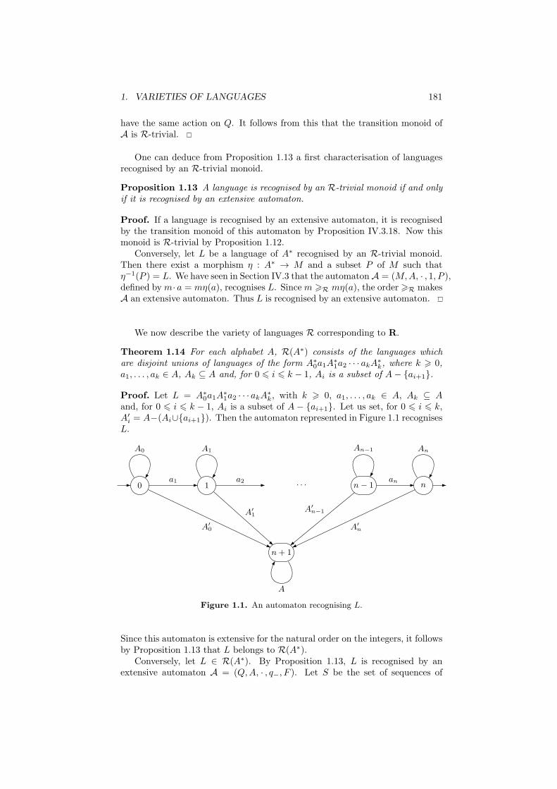
1. VARIETIES OF LANGUAGES 181
have the same action on Q. It follows from this that the transition monoid ofA is R-trivial.
One can deduce from Proposition 1.13 a first characterisation of languagesrecognised by an R-trivial monoid.
Proposition 1.13 A language is recognised by an R-trivial monoid if and onlyif it is recognised by an extensive automaton.
Proof. If a language is recognised by an extensive automaton, it is recognisedby the transition monoid of this automaton by Proposition IV.3.18. Now thismonoid is R-trivial by Proposition 1.12.
Conversely, let L be a language of A∗ recognised by an R-trivial monoid.Then there exist a morphism η : A∗ → M and a subset P of M such thatη−1(P ) = L. We have seen in Section IV.3 that the automatonA = (M,A, · , 1, P ),defined bym· a = mη(a), recognises L. Sincem >R mη(a), the order >R makesA an extensive automaton. Thus L is recognised by an extensive automaton.
We now describe the variety of languages R corresponding to R.
Theorem 1.14 For each alphabet A, R(A∗) consists of the languages whichare disjoint unions of languages of the form A∗
0a1A∗1a2 · · · akA
∗k, where k > 0,
a1, . . . , ak ∈ A, Ak ⊆ A and, for 0 6 i 6 k − 1, Ai is a subset of A− {ai+1}.
Proof. Let L = A∗0a1A
∗1a2 · · · akA
∗k, with k > 0, a1, . . . , ak ∈ A, Ak ⊆ A
and, for 0 6 i 6 k − 1, Ai is a subset of A − {ai+1}. Let us set, for 0 6 i 6 k,A′
i = A−(Ai∪{ai+1}). Then the automaton represented in Figure 1.1 recognisesL.
0 1 n− 1 n
n+ 1
a1 a2 an
A′0
A′1
A′n−1
A′n
A0 A1 An−1 An
A
. . .
Figure 1.1. An automaton recognising L.
Since this automaton is extensive for the natural order on the integers, it followsby Proposition 1.13 that L belongs to R(A∗).
Conversely, let L ∈ R(A∗). By Proposition 1.13, L is recognised by anextensive automaton A = (Q,A, · , q−, F ). Let S be the set of sequences of
182 CHAPTER IX. ALGEBRAIC CHARACTERISATIONS
the form (q0, a1, . . . , ak, qk) such that q0 < q1 < · · · < qn, q0 = q−, q0 · a1 =q1, . . . , qk−1 · ak = qk and qk ∈ F . Setting, for q ∈ Q, Aq = {a ∈ A | q · a = q},we claim that
L =⋃
(q0,a1,...,ak,qk)∈S
A∗q0a1A
∗q1 · · ·A
∗qk−1
akA∗qk. (1.1)
Note also that this union is disjoint since A is deterministic. Let K be the right-hand side of (1.1). If u ∈ K, there is a sequence (q0, a1, . . . , ak, qk) ∈ S and afactorisation u = u0a1u1 · · · akuk such that u0 ∈ A∗
q0 , . . . , uk ∈ A∗qk. It follows
that q0 ·u0 = q0, q0 · a1 = q1, . . . , qk−1 · ak = qk and qk ·uk = qk. Therefore,q0 ·u = qk and thus u ∈ L since q0 = q− and qk ∈ F .
Conversely, let u ∈ L. Since A is extensive, the successful path with label uvisits successively an increasing sequence of states q− = q0 < q1 < . . . < qk ∈ F .This gives a factorisation u = u0a1u1 · · · akuk, such that q0 ·u0 = q0, q0 · a1 = q1,. . . , qk−1 · ak = qk and qk ·uk = qk. Consequently, u belongs to K. This provesthe claim and the theorem.
A dual result holds for the variety of languages L corresponding to L.
Theorem 1.15 For each alphabet A, L(A∗) consists of the languages whichare disjoint unions of languages of the form A∗
0a1A∗1a2 · · · akA
∗k, where k > 0,
a1, . . . , ak ∈ A, A0 ⊆ A and, for 1 6 i 6 k, Ai is a subset of A− {ai}.
We conclude this section with a representation theorem for R-trivial monoids.Recall that a function f from an ordered set (E,6) into itself is extensive iffor all x ∈ E, x 6 f(x). Let En denote the submonoid of Tn consisting of allextensive functions from {1, . . . , n} into itself.
Proposition 1.16 For every n > 0, the monoid En is R-trivial.
Proof. Let f, g ∈ En such that f R g. There exist a, b ∈ En such that fa = gand gb = f . Let q ∈ {1, . . . , n}. Since a is extensive one has q · f 6 q · fa = q · gand likewise q · g 6 q · gb = q · f . It follows that f = g and thus En is R-trivial.
Theorem 1.17 A finite monoid is R-trivial if and only if it is a submonoid ofEn for some n > 0.
Proof. If M is R-trivial, the relation >R is a partial ordering. It follows that,for every m ∈M , the right translation ρm :M →M defined by ρm(x) = xm isextensive for this order. We have seen in Proposition II.4.25 that the functionm 7→ ρm is an injective morphism from M into T (M). Therefore, M is asubmonoid of En with n = |M |.
Conversely, suppose that M is a submonoid of En. Then En is R-trivial byProposition 1.16 and M is also R-trivial since the R-trivial monoids form avariety of monoids.
1.4 Some examples of +-varieties
Varieties corresponding to N, N+ and N−
Let N [N+, N−] denote the +-variety corresponding to N [N+, N−]. Recallthat a subset F of a set E is cofinite if the complement of F in E is finite.

1. VARIETIES OF LANGUAGES 183
Proposition 1.18 For each alphabet A,
(1) N+(A+) consists of the empty set and of the cofinite languages of A+,
(2) N−(A+) consists of A+ and of the finite languages of A+,
(3) N (A+) is the set of finite or cofinite languages of A+.
Proof. (1). Denote by ϕ : A+ → S the syntactic morphism of L. If L is empty,S is trivial, and thus belongs to N+. If L is a cofinite subset of A+, there existsan integer n such that L contains all the words of length > n. If u is such aword, we have xuy ∈ L for each x, y ∈ A∗, thereby showing that all the wordsof A+ of length > n are syntactically equivalent and have the same image eunder ϕ. Thus S is nilpotent by Proposition VII.4.14. Let now s ∈ S and letv ∈ ϕ−1(s). The formal implication
(xvy ∈ L⇒ xuy ∈ L)
shows that v 6L u, whence s 6 e in S. Therefore S ∈ N+.Conversely, let (S,6) ∈ N+, I an upper set of S and let ϕ : A+ → S be
a morphism of semigroups. If I is empty, ϕ−1(I) is also empty. Otherwise, Icontains necessarily 0, since 0 is maximal for 6. Let u be a word of lengthgreater than or equal to |S|. By Proposition VII.4.14, ϕ(u) = 0 and henceϕ(u) ∈ I. Therefore ϕ−1(I) is cofinite.
(2) follows from (1) by taking the complement.(3) What precedes shows that the syntactic semigroup of a finite or cofinite
subset is a nilpotent semigroup. To prove the converse, consider a nilpotentnonempty semigroup S. Let P be a subset of S and let ϕ : A+ → S be amorphism of semigroups. Then 0 belongs either to P , or to S − P and theargument above shows that ϕ−1(P ) is either finite or cofinite.
Varieties corresponding to ℓ1, r1 and L1
Let LI [ℓI, rI] denote the +-variety corresponding to L1 [ℓ1, r1].
Proposition 1.19 For each alphabet A, ℓI(A+) [rI(A+)] is the set of languagesof the form FA∗ ∪G [A∗F ∪G] where F and G are finite languages of A+. Itis also the Boolean algebra generated by the languages of the form uA∗ [A∗u].
Proof. Let L be a language of the form FA∗ ∪ G, where F and G are finitelanguages of A+. We claim that the syntactic semigroup of L belongs to ℓ1.Since the syntactic semigroup of G is nilpotent by Proposition 1.18, it suffices toconsider the syntactic semigroup S of the language FA∗. Let n be the maximumlength of the words of F and let u be a word of length greater than or equal ton. Then for every word v ∈ A∗, one has uv ∼FA∗ u, since the three conditionsxuvy ∈ FA∗, xu ∈ FA∗ and xuy ∈ FA∗ are clearly equivalent. It follows thatts = t for every t ∈ Sn and by Proposition VII.4.15, S belongs to ℓ1.
Conversely, let L be a language recognised by a semigroup S ∈ ℓ1 and letn = |S|. Then there exists a morphism ϕ : A+ → S such that L = ϕ−1(ϕ(L)).Let u be a word of L of length greater than or equal to n. Let us write u =vs with |v| = n and s ∈ A∗. By Proposition VII.4.15 (4), one has ϕ(u) =ϕ(v)ϕ(s) = ϕ(vA∗). It follows that L = FA∗ ∪G, where F is the set of wordsof L of length n and G is the set of words of L of length less than n.

184 CHAPTER IX. ALGEBRAIC CHARACTERISATIONS
The second part of the statement is easy to prove. First, we know thatℓI(A+) is a Boolean algebra and by the first part of the statement, it containsthe languages of the form uA∗, where u ∈ A+. Furthermore, the formula
{u} = uA∗ \ (⋃
a∈A
uaA∗)
shows that the Boolean algebra generated by the languages of the form uA∗ alsocontains the languages of the form {u}. Therefore, it contains the languages ofthe form FA∗ ∪G, with F and G finite.
Proposition 1.20 For each alphabet A, LI(A+) is the set of languages of theform FA∗G ∪ H where F , G and H are finite languages of A+. It is alsothe Boolean algebra generated by the languages of the form uA∗ or A∗u, whereu ∈ A+.
Proof. Let L be a language of the form FA∗G ∪ H, where F , G and H arefinite languages of A+. We claim that the syntactic semigroup of L belongsto L1. Since the syntactic semigroup of H is nilpotent by Proposition 1.18, itsuffices to consider the syntactic semigroup S of the language FA∗G. Let n bethe maximum length of the words of F and G and let u be a word of lengthgreater than or equal to n. Then for every word v ∈ A∗, one has uvu ∼FA∗G u,since the conditions xuvuy ∈ FA∗G and xuy ∈ FA∗G are clearly equivalent. Itfollows that tst = t for every t ∈ Sn and by Proposition VII.4.17, S belongs toL1.
Conversely, let L be a language recognised by a semigroup S ∈ L1 and letn = |S|. Then there exists a morphism ϕ : A+ → S such that L = ϕ−1(ϕ(L)).Let u be a word of L of length greater than or equal to 2n. Let us write u = pvswith |p| = |s| = n. By Proposition VII.4.17, one has ϕ(u) = ϕ(ps) = ϕ(pA∗s)and hence pA∗s ⊆ L. It follows that L is a finite union of languages of the formpA∗s, with |p| = |s| = n and of a set of words of length less than 2n.
For the second part of the statement, we know that LI(A+) is a Booleanalgebra and by the first part of the statement, it contains the languages of theform uA∗, A∗u, where u ∈ A+. Furthermore, the formula
{u} = (uA∗ ∩A∗u) \ (⋃
a∈A
uaA∗)
shows that the Boolean algebra generated by the languages of the form uA∗
or A∗u also contains the languages of the form {u}. Therefore, it contains thelanguages of the form FA∗G ∪H, with F , G and H finite.
2 Lattices of languages
We first give a number of examples of lattices of languages. We start by revisit-ing some classical examples studied between 1960 and 1980. Then we considersome more recent examples.
2. LATTICES OF LANGUAGES 185
2.1 The role of the zero
An element 0 of a monoid M is a zero if, for all m ∈ M , 0m = 0 = 0m. It iseasy to see that a monoid has at most one zero element. This allows one to usethe notation 0 for the zero without ambiguity. Observe that the trivial monoidhas a zero, but this is the only case for which 1 = 0. Also note that the minimalideal of a monoid with zero reduces to {0}. A quotient of a monoid with zeroalso has a zero, but this is not the case for a submonoid.
Languages with zero
A language with zero is a language whose syntactic monoid has a zero, or equiv-alently, a language fully recognised by a monoid with zero.
Proposition 2.21 The class of recognisable languages with zero is closed un-der Boolean operations and under quotients. It is not closed under inverses ofmorphisms, even for length-preserving morphisms.
Proof. Let C be the class of recognisable languages with zero. The emptylanguage and the full language belong to C, since their syntactic monoid istrivial. Proposition IV.2.8 shows that C is closed under complement. Let L1
and L2 be two languages of C and let ϕ1 : A∗ → M1 and ϕ2 : A∗ → M2
be their respective syntactic morphisms. By Proposition IV.2.9, L1 ∩ L2 isrecognised by the morphism ϕ : A∗ → Im(ϕ) ⊆ M1 ×M2 defined by ϕ(u) =(ϕ1(u1), ϕ2(u2)). We claim that the monoid M = Im(ϕ) has a zero. Indeed,let u1 and u2 be words such that ϕ1(u1) = 0 and ϕ2(u2) = 0. Then theelement ϕ(u1u2) is a zero of M . Indeed, if ϕ(u) is an element of M , thenϕ(u)ϕ(u1u2) = ϕ(uu1u2) = (ϕ1(uu1u2), ϕ2(uu1u2)) = (0, 0) = ϕ(u1u2) andsimilarly, ϕ(u1u2)ϕ(u) = ϕ(u1u2). This proves the claim and shows that L1∩L2
is a language with zero. Thus C is closed under Boolean operations.Let L be a recognisable language with zero and letM be its syntactic monoid.
Let u be a word of A∗. It follows from Proposition IV.2.11 that the languagesu−1L and Lu−1 are also recognised by M . It follows that the syntactic monoidof these languages is a quotient of M and hence has a zero. Thus C is closedunder quotients.
Finally let A = {a, b} and let ϕ : A∗ → A∗ be the length-preserving mor-phism defined by ϕ(a) = ϕ(b) = a. If L = (a2)∗, then ϕ−1(L) = (A2)∗. NowL has a zero, but the syntactic monoid of (A2)∗ is the cyclic group of order 2,which has no zero.
According to Corollary VIII.3.12, the class of recognisable languages withzero has an equational definition, but finding one explicitly requires a little bitof work.
Let us fix a total order on the alphabet A. Let u0, u1, . . . be the orderedsequence of all words of A+ in the induced shortlex order. For instance, ifA = {a, b} with a < b, the first elements of this sequence would be
1, a, b, aa, ab, ba, bb, aaa, aab, aba, abb, baa, bab, bba, bbb, aaaa, . . .
It is proved in [125, 5] that the sequence of words (vn)n>0 defined by
v0 = u0, vn+1 = (vnun+1vn)(n+1)!

186 CHAPTER IX. ALGEBRAIC CHARACTERISATIONS
converges to an idempotent ρA of the minimal ideal of the free profinite monoidon A. This profinite element can be used to give an equational characterisationof the recognisable languages with zero.
Proposition 2.22 A recognisable language has a zero if and only if it satisfiesthe equation xρA = ρA = ρAx for all x ∈ A∗.
Proof. Let L be a recognisable language and let η : A∗ → M be its syntacticmonoid. Since ρA belongs to the minimal ideal of A∗, η(ρA) is an element of theminimal ideal of M . In particular, if M has a zero, η(ρA) = 0 and L satisfiesthe equations xρA = ρA = ρAx for all x ∈ A∗.
Conversely, assume that L satisfies these equations. Let m ∈ M and letx ∈ A∗ be such that η(x) = m. Then the equations η(xρA) = η(ρA) = η(ρAx)give mη(ρA) = η(ρA) = η(ρA)m, showing that η(ρA) is a zero of M . Thus Lhas a zero.
In the sequel, we shall use freely the symbol 0 in equations to mean thata monoid has a zero. For instance the equation 0 6 x of Theorem 2.25 belowshould be formally replaced by the two equations xρA = ρA = ρAx and ρA 6 x.
Nondense languages
A language L of A∗ is dense if, for every word u ∈ A∗, L ∩ A∗uA∗ 6= ∅, or,equivalently, if (A∗)−1L(A∗)−1 = A∗. Note that dense languages are not closedunder intersection: (A2)∗ and (A2)∗A ∪ {1} are dense, but their intersection isnot dense.
Proposition 2.23 Nondense or full languages are closed under finite union,finite intersection and left and right quotients.
Proof. Let L1 and L2 be two nondense languages of A∗. Then there exist twowords u1, u2 ∈ A∗ such that L1 ∩A∗u1A
∗ = ∅ and L1 ∩A∗u2A∗ = ∅. It follows
that (L1 ∩L2)∩A∗u1A
∗ = ∅ and (L1 ∪L2)∩A∗u1u2A
∗ = ∅. Thus L1 ∩L2 andL1 ∪ L2 are nondense. If L1 = A∗, then L1 ∩ L2 = L2 and L1 ∪ L2 = A∗. Thusnondense or full languages are closed under finite union and finite intersection.
Let L be a nondense language. Then there exists a word u ∈ A∗ such thatL∩A∗uA∗ = ∅. Let x, y ∈ A∗. We claim that x−1Ly−1∩A∗uA∗ = ∅. Otherwise,there exist two words s, t such that sut ∈ x−1Ly−1. It follows that xsuty ∈ L, acontradiction, since L∩A∗uA∗ = ∅. Thus x−1Ly−1 is nondense. If L = A∗, thenx−1Ly−1 = A∗ for all words x, y ∈ A∗. Therefore nondense or full languagesare closed under left and right quotients.
Proposition 2.24 Nondense or full languages are not closed under inverses ofmorphisms, even for length-preserving morphisms.
Proof. Let ϕ : {a, b}∗ → {a, b}∗ be the morphism defined by ϕ(a) = ϕ(b) = a.Then a+ is nondense in {a, b}∗, but ϕ−1(a+) = {a, b}+ is dense and not full.
We now give an equational description of nondense or full languages of the formforetold by Theorem VIII.3.10.

2. LATTICES OF LANGUAGES 187
Theorem 2.25 A language of A∗ is nondense or full if and only if it satisfiesthe identity 0 6 x.
Proof. Let L be a recognisable language of A∗, let η : A∗ →M be its syntacticmonoid and P its syntactic image. First observe that the identity 0 6 x meansthat if 0 ∈ P , then P =M and hence M = {0} since M is the syntactic monoidof P .
Suppose that L is nondense. Then there exists a word u ∈ A∗ such thatL∩A∗uA∗ = ∅. It follows that for all x ∈ A∗, xu ∼L u ∼L ux and hence η(u) isa zero in M . Furthermore 0 /∈ P . If now L is full, then M is the trivial monoidwhich has a zero. Thus the identity is satisfied in both cases.
Conversely, assume that M satisfies the identity 0 6 x. Then M has a zero.If 0 ∈ P , then M is the trivial monoid and L is full. Otherwise, 0 /∈ P . Let ube a word such that η(u) = 0. Then η(A∗uA∗) = 0 and hence L ∩ A∗uA∗ = ∅.Thus L is nondense.
2.2 Languages defined by density
The density of a language L ⊆ A∗ is the function which counts the number ofwords of length n in L. More formally, it is the function dL : N→ N defined by
dL(n) = |L ∩An|
where |E| denotes the cardinality of a set E. We first state some elementaryproperties of this function.
Proposition 2.26 Let L1 and L2 be two languages. Then, for all n,
(1) dL1∪L2(n) 6 dL1
(n) + dL2(n),
(2) dL1∩L2(n) 6 min{dL1
(n), dL2(n)},
(3) dL1L2(n) 6
∑06k6n dL1
(k)dL2(n− k).
Proof. The double relation
(L1 ∩ L2) ∩An ⊆ (L1 ∪ L2) ∩A
n = (L1 ∩An) ∪ (L2 ∩A
n)
gives immediately (1) and (2). Relation (3) follows from the fact that L1L2∩An
is the union of the languages (L1 ∩Ak)(L2 ∩A
n−k), for 0 6 k 6 n.
If dL(n) = O(1), then L is called a slender language. A language that hasat most one word of each length is called a thin language. Finally, a language issparse if it has a polynomial density, that is, if dL(n) = O(nk) for some k > 0.See [165] for a general reference.
Slender languages
Recognisable slender languages have a simple description (see [165, Theorem3.6]).
Theorem 2.27 A recognisable language is slender if and only if it is a finiteunion of languages of the form xu∗y, where x, u, y ∈ A∗.

188 CHAPTER IX. ALGEBRAIC CHARACTERISATIONS
Not that if |A| 6 1, all recognisable languages are slender. This is trivial ifthe alphabet is empty. If A = {a}, every recognisable language of A∗ is a finiteunion of languages of the form xu∗y since ak = ak1∗1, and aka∗ = aka∗1.
Since we only consider lattices of recognisable languages, we are interestedin the class of recognisable languages which are either slender or full. We firststudy their closure properties.
Proposition 2.28 Recognisable slender languages are closed under finite union,finite intersection, quotients and morphisms.
Proof. Since any language contained in a slender language is also slender, recog-nisable slender languages are closed under finite intersection. Closure underfinite union is a direct consequence of Theorem 2.27. Closure under morphismsis trivial.
Let a be a letter of A and let x, u, y be words of A∗. Then
a−1(xu∗y) =
(a−1x)u∗y if x 6= 1,
(a−1u)u∗y if x = 1 and u 6= 1,
a−1y if x = 1 and u = 1.
Therefore a−1(xu∗y) is a recognisable slender language in all cases. It followsnow from Theorem 2.27 that recognisable slender languages are closed underleft quotient by letters, and, by induction, by any word. The proof for rightquotients is similar.
Corollary 2.29 Suppose that |A| > 2. Then any recognisable slender languageof A∗ is nondense.
Proof. Let L be a recognisable slender language. Then by Proposition 2.28,the language (A∗)−1L(A∗)−1 is also slender. Since |A| > 2, this language cannotbe equal to A∗. Therefore L is nondense.
Proposition 2.30 Recognisable slender languages are not closed under inversesof morphisms, even for length-preserving morphisms.
Proof. We use the same example as for Proposition 2.24. Let ϕ : {a, b}∗ →{a, b}∗ be the morphism defined by ϕ(a) = ϕ(b) = a. Then a+ is slender in{a, b}∗, but ϕ−1(a+) = {a, b}+ is nor slender nor full.
Recall that a cycle in a directed graph is a path such that the start vertexand end vertex are the same. A simple cycle is a closed directed path, withno repeated vertices other than the starting and ending vertices. The followingresult is folklore, but we give a self-contained proof for the convenience of thereader.
Theorem 2.31 Let L be a recognisable language and let A be its minimal de-terministic trim automaton. The following conditions are equivalent:
(1) L is slender,
(2) A does not contain any connected pair of cycles,
(3) A does not contain any connected pair of simple cycles.
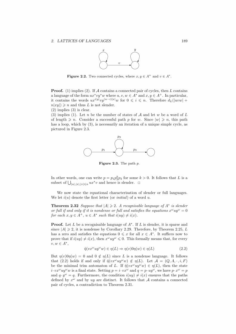
2. LATTICES OF LANGUAGES 189
v
x y
Figure 2.2. Two connected cycles, where x, y ∈ A+ and v ∈ A∗.
Proof. (1) implies (2). If A contains a connected pair of cycles, then L containsa language of the form ux∗vy∗w where u, v, w ∈ A∗ and x, y ∈ A+. In particular,it contains the words uxi|y|vy(n−i)|x|w for 0 6 i 6 n. Therefore dL(|uvw| +n|xy|) > n and thus L is not slender.(2) implies (3) is clear.(3) implies (1). Let n be the number of states of A and let w be a word of Lof length > n. Consider a successful path p for w. Since |w| > n, this pathhas a loop, which by (3), is necessarily an iteration of a unique simple cycle, aspictured in Figure 2.3.
p1
p2
p3
Figure 2.3. The path p.
In other words, one can write p = p1pk2p3 for some k > 0. It follows that L is a
subset of⋃
|u|,|x|,|v|6n ux∗v and hence is slender.
We now state the equational characterisation of slender or full languages.We let i(u) denote the first letter (or initial) of a word u.
Theorem 2.32 Suppose that |A| > 2. A recognisable language of A∗ is slenderor full if and only if it is nondense or full and satisfies the equations xωuyω = 0for each x, y ∈ A+, u ∈ A∗ such that i(uy) 6= i(x).
Proof. Let L be a recognisable language of A∗. If L is slender, it is sparse andsince |A| > 2, it is nondense by Corollary 2.29. Therefore, by Theorem 2.25, Lhas a zero and satisfies the equations 0 6 x for all x ∈ A∗. It suffices now toprove that if i(uy) 6= i(x), then xωuyω 6 0. This formally means that, for everyv, w ∈ A∗,
η(vxωuyωw) ∈ η(L)⇒ η(v)0η(w) ∈ η(L) (2.2)
But η(v)0η(w) = 0 and 0 /∈ η(L) since L is a nondense language. It followsthat (2.2) holds if and only if η(vxωuyωw) /∈ η(L). Let A = (Q,A, · , i, F )be the minimal trim automaton of L. If η(vxωuyωw) ∈ η(L), then the statei· vxωuyωw is a final state. Setting p = i· vxω and q = p·uyω, we have p·xω = pand q · yω = q. Furthermore, the condition i(uy) 6= i(x) ensures that the pathsdefined by xω and by uy are distinct. It follows that A contains a connectedpair of cycles, a contradiction to Theorem 2.31.

190 CHAPTER IX. ALGEBRAIC CHARACTERISATIONS
Suppose now that L is neither slender nor full and let A be the minimalautomaton of L. By Theorem 2.31, A contains a connected pair of simplecycles. Therefore, there exist some words x, y ∈ A+, u0, u1, u2 ∈ A
∗ such thati(u1y) 6= i(x) and u0x
∗u1y∗u2 ⊆ L. It follows that η(u0x
ωu1yωu2) ∈ η(L) and
thus L does not satisfy the equation xωu1yω 6 0.
Let us add two comments to this result. First, on a one letter alphabet,every recognisable language is slender, but not necessarily nondense or full: onthe alphabet {a}, the language a+ is slender, dense, but not full. Second, itlooks a little bit suspicious to characterise a class of languages which is notclosed under complement by equations of the form u = v and not by equationsof the form u 6 v, as Theorem VIII.3.10 would suggest. The explanation lies inthe first condition, “nondense or full”, which, by Theorem 2.25, can be definedby equations of the form 0 6 x.
We now consider the Boolean closure of slender languages. A language iscalled coslender if its complement is slender.
Proposition 2.33 Recognisable slender or coslender languages are closed underBoolean operations. They are also closed under quotients but not under inversesof morphisms, even for length-preserving morphisms.
Proof. Let C be the class of recognisable slender or coslender languages. It isclearly closed under complement. Let L1, L2 ∈ C. If L1 and L2 are both slender,then L1 ∩ L2 is also slender by Proposition 2.28. Suppose now that L1 and L2
are coslender. Then Lc1 and Lc
2 are slender and so is their union by Theorem2.27. Since (L1 ∩ L2)
c = Lc1 ∪ L
c2, it follows that L1 ∩ L2 is coslender. Thus C
is closed under finite intersection and hence under Boolean operations.Since slender languages are closed under quotients and since quotients com-
mute with complement (in the sense that u−1Lc = (u−1L)c) C is closed underquotients.
Finally, let ϕ : {a, b, c}∗ → {a, b, c}∗ be the morphism defined by ϕ(a) =ϕ(b) = a and ϕ(c) = c. Then a+ is slender in {a, b}∗, but ϕ−1(a+) = {a, b}+ isnor slender nor coslender.
We now come to the equational characterisation.
Theorem 2.34 Suppose that |A| > 2. A recognisable language of A∗ is slenderor coslender if and only if its syntactic monoid has a zero and satisfies theequations xωuyω = 0 for each x, y ∈ A+, u ∈ A∗ such that i(uy) 6= i(x).
Proof. This is an immediate consequence of Theorem 2.32.
Note that if A = {a}, the language (a2)∗ is slender but its syntactic monoid,the cyclic group of order 2, has no zero. Therefore the condition |A| > 2 inTheorem 2.34 is mandatory.
Sparse languages
The closure properties of sparse languages are similar to that of slender lan-guages. See [165, Theorem 3.8].
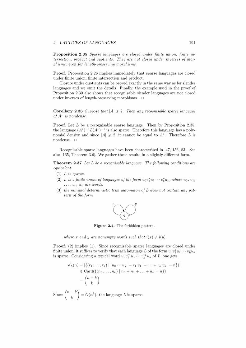
2. LATTICES OF LANGUAGES 191
Proposition 2.35 Sparse languages are closed under finite union, finite in-tersection, product and quotients. They are not closed under inverses of mor-phisms, even for length-preserving morphisms.
Proof. Proposition 2.26 implies immediately that sparse languages are closedunder finite union, finite intersection and product.
Closure under quotients can be proved exactly in the same way as for slenderlanguages and we omit the details. Finally, the example used in the proof ofProposition 2.30 also shows that recognisable slender languages are not closedunder inverses of length-preserving morphisms.
Corollary 2.36 Suppose that |A| > 2. Then any recognisable sparse languageof A∗ is nondense.
Proof. Let L be a recognisable sparse language. Then by Proposition 2.35,the language (A∗)−1L(A∗)−1 is also sparse. Therefore this language has a poly-nomial density and since |A| > 2, it cannot be equal to A∗. Therefore L isnondense.
Recognisable sparse languages have been characterised in [47, 156, 83]. Seealso [165, Theorem 3.6]. We gather these results in a slightly different form.
Theorem 2.37 Let L be a recognisable language. The following conditions areequivalent:
(1) L is sparse,
(2) L is a finite union of languages of the form u0v∗1u1 · · · v
∗kuk, where u0, v1,
. . . , vk, uk are words.
(3) the minimal deterministic trim automaton of L does not contain any pat-tern of the form
q
yx
Figure 2.4. The forbidden pattern.
where x and y are nonempty words such that i(x) 6= i(y).
Proof. (2) implies (1). Since recognisable sparse languages are closed underfinite union, it suffices to verify that each language L of the form u0v
∗1u1 · · · v
∗kuk
is sparse. Considering a typical word u0vr11 u1 · · · v
rkk uk of L, one gets
dL(n) = |{(r1, . . . , rk) | |u0 · · ·uk|+ r1|v1|+ . . .+ rk|vk| = n})|
6 Card({(n0, . . . , nk) | n0 + n1 + . . .+ nk = n})
=
(n+ k
k
)
Since
(n+ k
k
)= O(nk), the language L is sparse.
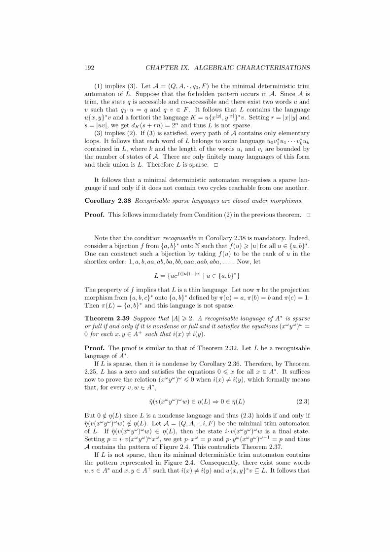
192 CHAPTER IX. ALGEBRAIC CHARACTERISATIONS
(1) implies (3). Let A = (Q,A, · , q0, F ) be the minimal deterministic trimautomaton of L. Suppose that the forbidden pattern occurs in A. Since A istrim, the state q is accessible and co-accessible and there exist two words u andv such that q0 ·u = q and q · v ∈ F . It follows that L contains the languageu{x, y}∗v and a fortiori the language K = u{x|y|, y|x|}∗v. Setting r = |x||y| ands = |uv|, we get dK(s+ rn) = 2n and thus L is not sparse.
(3) implies (2). If (3) is satisfied, every path of A contains only elementaryloops. It follows that each word of L belongs to some language u0v
∗1u1 · · · v
∗kuk
contained in L, where k and the length of the words ui and vi are bounded bythe number of states of A. There are only finitely many languages of this formand their union is L. Therefore L is sparse.
It follows that a minimal deterministic automaton recognises a sparse lan-guage if and only if it does not contain two cycles reachable from one another.
Corollary 2.38 Recognisable sparse languages are closed under morphisms.
Proof. This follows immediately from Condition (2) in the previous theorem.
Note that the condition recognisable in Corollary 2.38 is mandatory. Indeed,consider a bijection f from {a, b}∗ onto N such that f(u) > |u| for all u ∈ {a, b}∗.One can construct such a bijection by taking f(u) to be the rank of u in theshortlex order: 1, a, b, aa, ab, ba, bb, aaa, aab, aba, . . . . Now, let
L = {ucf(|u|)−|u| | u ∈ {a, b}∗}
The property of f implies that L is a thin language. Let now π be the projectionmorphism from {a, b, c}∗ onto {a, b}∗ defined by π(a) = a, π(b) = b and π(c) = 1.Then π(L) = {a, b}∗ and this language is not sparse.
Theorem 2.39 Suppose that |A| > 2. A recognisable language of A∗ is sparseor full if and only if it is nondense or full and it satisfies the equations (xωyω)ω =0 for each x, y ∈ A+ such that i(x) 6= i(y).
Proof. The proof is similar to that of Theorem 2.32. Let L be a recognisablelanguage of A∗.
If L is sparse, then it is nondense by Corollary 2.36. Therefore, by Theorem2.25, L has a zero and satisfies the equations 0 6 x for all x ∈ A∗. It sufficesnow to prove the relation (xωyω)ω 6 0 when i(x) 6= i(y), which formally meansthat, for every v, w ∈ A∗,
η(v(xωyω)ωw) ∈ η(L)⇒ 0 ∈ η(L) (2.3)
But 0 /∈ η(L) since L is a nondense language and thus (2.3) holds if and only ifη(v(xωyω)ωw) /∈ η(L). Let A = (Q,A, · , i, F ) be the minimal trim automatonof L. If η(v(xωyω)ωw) ∈ η(L), then the state i· v(xωyω)ωw is a final state.Setting p = i· v(xωyω)ωxω, we get p·xω = p and p· yω(xωyω)ω−1 = p and thusA contains the pattern of Figure 2.4. This contradicts Theorem 2.37.
If L is not sparse, then its minimal deterministic trim automaton containsthe pattern represented in Figure 2.4. Consequently, there exist some wordsu, v ∈ A∗ and x, y ∈ A+ such that i(x) 6= i(y) and u{x, y}∗v ⊆ L. It follows that

2. LATTICES OF LANGUAGES 193
η(u(xωyω)ωv) ∈ η(L) and thus L does not satisfy the equation u(xωyω)ωv 60.
Pursuing the analogy with slender languages, we consider now the Booleanclosure of sparse languages. A language is called cosparse if its complement issparse.
Theorem 2.40 Suppose that |A| > 2. A recognisable language of A∗ is sparseor cosparse if and only if its syntactic monoid has a zero and satisfies the equa-tions (xωyω)ω = 0 for each x, y ∈ A+ such that i(x) 6= i(y).
Proof. This is an immediate consequence of Theorem 2.39.
2.3 Cyclic and strongly cyclic languages
Cyclic languages
A language is cyclic if it is closed under conjugation, power and root. Thus Lis cyclic if and only if, for all u, v ∈ A∗ and n > 0,
(1) un ∈ L if and only if u ∈ L,
(2) uv ∈ L if and only if vu ∈ L.
Let L ∈ Rec(A∗), let ϕ : A∗ →M be a surjective morphism fully recognising Land let P = η(L). A direct translation of the definition shows that a recognisablelanguage is cyclic if and only if it satisfies, for all x, y ∈M and n > 0,
(xy ∈ P ⇐⇒ yx ∈ P ) and (xn ∈ P ⇐⇒ x ∈ P )
With the notation of Section VIII.1, we get:
Proposition 2.41 A recognisable language is cyclic if and only if it satisfiesthe identities xy ↔ yx and xω ↔ x.
The closure properties of cyclic languages are summarised as follows.
Proposition 2.42 Recognisable cyclic languages are closed under inverses ofmorphisms and under Boolean operations but not under quotients.
Proof. The first part of the statement follows from Theorem VIII.4.14 andProposition 2.41. Furthermore, the language L = {abc, bca, cab} is cyclic, butits quotient a−1L = {bc} is not cyclic.
Here is a useful property of the groups of a monoid fully recognising a cycliclanguage. This property holds of course for the syntactic monoid but we shallneed this slightly more general result in the proof of Theorem 2.52.
Proposition 2.43 Let M be a monoid fully recognising a recognisable cycliclanguage L and let H be a group of M . Let also P be the image of L in M .Then either H and P are disjoint or H is a subset of P . In the latter case, allthe groups in the D-class of H are also contained in P .
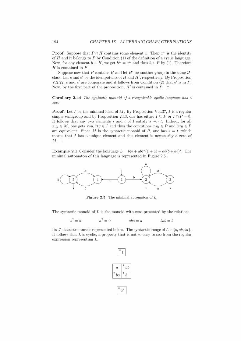
194 CHAPTER IX. ALGEBRAIC CHARACTERISATIONS
Proof. Suppose that P ∩H contains some element x. Then xω is the identityof H and it belongs to P by Condition (1) of the definition of a cyclic language.Now, for any element h ∈ H, we get hω = xω and thus h ∈ P by (1). ThereforeH is contained in P .
Suppose now that P contains H and let H ′ be another group in the same D-class. Let e and e′ be the idempotents ofH andH ′, respectively. By PropositionV.2.22, e and e′ are conjugate and it follows from Condition (2) that e′ is in P .Now, by the first part of the proposition, H ′ is contained in P .
Corollary 2.44 The syntactic monoid of a recognisable cyclic language has azero.
Proof. Let I be the minimal ideal of M . By Proposition V.4.37, I is a regularsimple semigroup and by Proposition 2.43, one has either I ⊆ P or I ∩ P = ∅.It follows that any two elements s and t of I satisfy s ∼P t. Indeed, for allx, y ∈ M , one gets xsy, xty ∈ I and thus the conditions xsy ∈ P and xty ∈ Pare equivalent. Since M is the syntactic monoid of P , one has s = t, whichmeans that I has a unique element and this element is necessarily a zero ofM .
Example 2.1 Consider the language L = b(b+ ab)∗(1 + a) + ab(b+ ab)∗. Theminimal automaton of this language is represented in Figure 2.5.
1 2 345b
a
b
a
b
a
b
b
Figure 2.5. The minimal automaton of L.
The syntactic monoid of L is the monoid with zero presented by the relations
b2 = b a2 = 0 aba = a bab = b
Its J -class structure is represented below. The syntactic image of L is {b, ab, ba}.It follows that L is cyclic, a property that is not so easy to see from the regularexpression representing L.
∗1
a∗ab
∗ba∗b
∗a2
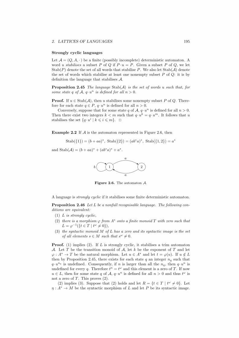
2. LATTICES OF LANGUAGES 195
Strongly cyclic languages
Let A = (Q,A, · ) be a finite (possibly incomplete) deterministic automaton. Aword u stabilises a subset P of Q if P ·u = P . Given a subset P of Q, we letStab(P ) denote the set of all words that stabilise P . We also let Stab(A) denotethe set of words which stabilise at least one nonempty subset P of Q: it is bydefinition the language that stabilises A.
Proposition 2.45 The language Stab(A) is the set of words u such that, forsome state q of A, q ·un is defined for all n > 0.
Proof. If u ∈ Stab(A), then u stabilises some nonempty subset P of Q. There-fore for each state q ∈ P , q ·un is defined for all n > 0.
Conversely, suppose that for some state q of A, q ·un is defined for all n > 0.Then there exist two integers k < m such that q ·uk = q ·um. It follows that ustabilises the set {q ·ui | k 6 i 6 m}.
Example 2.2 If A is the automaton represented in Figure 2.6, then
Stab({1}) = (b+ aa)∗, Stab({2}) = (ab∗a)∗, Stab({1, 2}) = a∗
and Stab(A) = (b+ aa)∗ + (ab∗a)∗ + a∗.
1 2
a
a
b
Figure 2.6. The automaton A.
A language is strongly cyclic if it stabilises some finite deterministic automaton.
Proposition 2.46 Let L be a nonfull recognisable language. The following con-ditions are equivalent:
(1) L is strongly cyclic,
(2) there is a morphism ϕ from A∗ onto a finite monoid T with zero such thatL = ϕ−1({t ∈ T | tω 6= 0}),
(3) the syntactic monoid M of L has a zero and its syntactic image is the setof all elements s ∈M such that sω 6= 0.
Proof. (1) implies (2). If L is strongly cyclic, it stabilises a trim automatonA. Let T be the transition monoid of A, let k be the exponent of T and letϕ : A∗ → T be the natural morphism. Let u ∈ A∗ and let t = ϕ(u). If u /∈ Lthen by Proposition 2.45, there exists for each state q an integer nq such thatq ·unq is undefined. Consequently, if n is larger than all the nq, then q ·un isundefined for every q. Therefore tn = tω and this element is a zero of T . If nowu ∈ L, then for some state q of A, q ·un is defined for all n > 0 and thus tω isnot a zero of T . This proves (2).
(2) implies (3). Suppose that (2) holds and let R = {t ∈ T | tω 6= 0}. Letη : A∗ → M be the syntactic morphism of L and let P be its syntactic image.
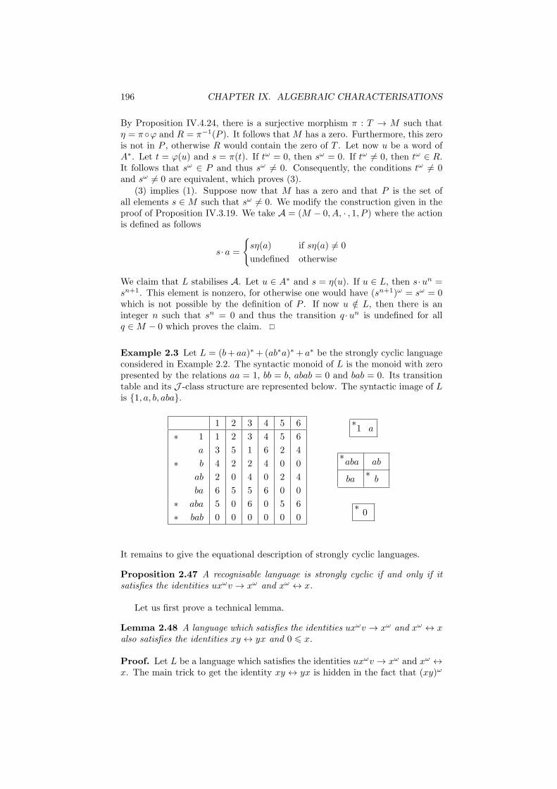
196 CHAPTER IX. ALGEBRAIC CHARACTERISATIONS
By Proposition IV.4.24, there is a surjective morphism π : T → M such thatη = π◦ϕ and R = π−1(P ). It follows thatM has a zero. Furthermore, this zerois not in P , otherwise R would contain the zero of T . Let now u be a word ofA∗. Let t = ϕ(u) and s = π(t). If tω = 0, then sω = 0. If tω 6= 0, then tω ∈ R.It follows that sω ∈ P and thus sω 6= 0. Consequently, the conditions tω 6= 0and sω 6= 0 are equivalent, which proves (3).
(3) implies (1). Suppose now that M has a zero and that P is the set ofall elements s ∈ M such that sω 6= 0. We modify the construction given in theproof of Proposition IV.3.19. We take A = (M − 0, A, · , 1, P ) where the actionis defined as follows
s· a =
{sη(a) if sη(a) 6= 0
undefined otherwise
We claim that L stabilises A. Let u ∈ A∗ and s = η(u). If u ∈ L, then s·un =sn+1. This element is nonzero, for otherwise one would have (sn+1)ω = sω = 0which is not possible by the definition of P . If now u /∈ L, then there is aninteger n such that sn = 0 and thus the transition q ·un is undefined for allq ∈M − 0 which proves the claim.
Example 2.3 Let L = (b+ aa)∗ +(ab∗a)∗ + a∗ be the strongly cyclic languageconsidered in Example 2.2. The syntactic monoid of L is the monoid with zeropresented by the relations aa = 1, bb = b, abab = 0 and bab = 0. Its transitiontable and its J -class structure are represented below. The syntactic image of Lis {1, a, b, aba}.
1 2 3 4 5 6
∗ 1 1 2 3 4 5 6
a 3 5 1 6 2 4
∗ b 4 2 2 4 0 0
ab 2 0 4 0 2 4
ba 6 5 5 6 0 0
∗ aba 5 0 6 0 5 6
∗ bab 0 0 0 0 0 0
∗1 a
∗aba ab
ba∗b
∗0
It remains to give the equational description of strongly cyclic languages.
Proposition 2.47 A recognisable language is strongly cyclic if and only if itsatisfies the identities uxωv → xω and xω ↔ x.
Let us first prove a technical lemma.
Lemma 2.48 A language which satisfies the identities uxωv → xω and xω ↔ xalso satisfies the identities xy ↔ yx and 0 6 x.
Proof. Let L be a language which satisfies the identities uxωv → xω and xω ↔x. The main trick to get the identity xy ↔ yx is hidden in the fact that (xy)ω
2. LATTICES OF LANGUAGES 197
and (yx)ω are conjugate. More precisely, the derivation
xy ↔ (xy)ω = (xy)ω(xy)ω = (xy)ω−1xy(xy)ω−1xy
= ((xy)ω−1x)(yx)ωy → (yx)ω ↔ yx
shows that xy → yx and the opposite identity yx→ xy follows by symmetry.Theorem 2.25 shows that L satisfies the identity 0 6 x if and only if it is
nondense or full. Let n be the exponent of L. Suppose that L is not full andlet us prove that it is nondense. Let x /∈ L. We claim that for all u, v ∈ A∗,uxnv /∈ L. Indeed, if uxnv ∈ L, the identity uxωv → xω gives xn ∈ L and theidentity xω ↔ x gives x ∈ L, a contradiction. This proves the claim and thelemma.
Let us now come back to the proof of Proposition 2.47.
Proof. Let L be a recognisable strongly cyclic language, let M be its syntacticmonoid and let P be its syntactic image. Lemma 2.48 shows that L has a zero.Observing that xω = (xω)ω, one gets
x ∈ P ⇐⇒ xω 6= 0⇐⇒ (xω)ω 6= 0⇐⇒ xω ∈ P
which proves that L satisfies the identity xω ↔ x. Finally, if uxωv ∈ P , then(uxωv)ω 6= 0. Therefore xω 6= 0, whence x ∈ P and finally xω ∈ P since xω ↔ x.Thus L satisfies the identity uxωv → xω.
Conversely, suppose that L satisfies the two identities of the statement. ByLemma 2.48, M has a zero and 0 /∈ P . By Proposition 2.46, it suffices to provethat x ∈ P if and only if xω 6= 0. First, if x ∈ P , then xω ∈ P and since 0 /∈ P ,one has xω 6= 0. Now, if xω 6= 0, then uxωv ∈ P for some u, v ∈M (since xω isnot equivalent to 0 in the syntactic equivalence of P ). It follows xω ∈ P by thefirst identity and x ∈ P by the second one.
The next corollaries allows a precise comparison between cyclic and stronglycyclic languages.
Corollary 2.49 Any recognisable strongly cyclic language is cyclic.
Proof. It suffices to prove that a recognisable strongly cyclic language alsosatisfies the identity xy ↔ yx. Indeed, for each x, y ∈ M , (xy)ω and (yx)ω aretwo conjugate idempotents. It follows that (xy)ω 6= 0 if and only if (yx)ω 6= 0.
Corollary 2.50 Let L be a recognisable cyclic language. Let M be its syntacticmonoid and let P be its syntactic image. Then L is strongly cyclic if and onlyif for all idempotent e, f of M , the conditions e ∈ P and e 6J f imply f ∈ P .
The proof is again a typical exercise on identities.
Proof. Let ϕ : A∗ → M be the syntactic morphism of L. Suppose that L isstrongly cyclic and let e, f be two idempotents of M such that e 6J f . Also lets, t ∈M be such that e = sft. Lifting up to A∗, one can find words x, y, u, v suchthat ϕ(x) = e, ϕ(y) = f , ϕ(u) = s and ϕ(v) = t. By Proposition 2.47, L satisfiesthe identities (a) uxωv → xω and (b) xω ↔ x. Now ϕ(uyωv)ω = sft = e ∈ P ,

198 CHAPTER IX. ALGEBRAIC CHARACTERISATIONS
and thus by (b) ϕ(uyωv) ∈ P . Since ϕ(uyωv) = ϕ(u)ϕ(y)ωϕ(v), it follows by(a) that ϕ(y)ω ∈ P and thus f ∈ P .
In the opposite direction, suppose that for all idempotents e, f of M , theconditions e ∈ P and e 6J f imply f ∈ P . Since L is cyclic it satisfiesthe identity xω ↔ x by Proposition 2.41. We claim that it also satisfies theidentity uxωv → xω. First, ϕ(uxωv) ∈ P implies ϕ(uxωv)ω ∈ P since xω ↔ x.Furthermore, since ϕ(uxωv)ω 6J ϕ(xω), one also has ϕ(xω) ∈ P , which finallygives ϕ(x) ∈ P since xω ↔ x.
Proposition 2.51 Recognisable strongly cyclic languages are closed under in-verses of morphisms, finite intersection and finite union but not under quotients.
Proof. Theorem VIII.4.14 and Proposition 2.47 show that strongly cyclic lan-guages form a positive stream of languages. It remains to show that there arenot closed under quotients. The language L = (b+aa)∗+(ab∗a)∗+a∗ of Exam-ple 2.3 is strongly cyclic. However, its quotient b−1L = (b+aa)∗ is not stronglycyclic, since aa ∈ (b+ aa)∗ but a /∈ (b+ aa)∗.
We now give the connexion between cyclic and strongly cyclic languages.
Theorem 2.52 A recognisable language is cyclic if and only if it is a Booleancombination of recognisable strongly cyclic languages.
Proof. Propositions 2.41 and 2.47 and the remark preceeding Proposition 2.51show that a Boolean combination of recognisable strongly cyclic language iscyclic.
We now show that any cyclic language L is a Boolean combination of recog-nisable strongly cyclic languages. The proof is by induction on the size of amonoid with zero fully recognising L. Such a monoid always exists, since byCorollary 2.44, the syntactic monoid of L has a zero.
Let T be a monoid with zero, let ϕ : A∗ → T be a surjective morphismrecognising L and let P = ϕ(L). We may also assume that 0 /∈ P . Otherwise,observing that 0 /∈ P c, it suffices to prove the result for Lc, which is also cyclicand fully recognised by ϕ.
If T is trivial, then 1 = 0 and P is empty. Thus L is necessarily the emptylanguage, which is strongly cyclic since it stabilises the empty automaton. Sup-pose now that T is nontrivial. Let us set
R = {t ∈ T | tω 6= 0}, S = R− P, U = ϕ−1(R) and V = U − L
Proposition 2.46 shows that U is strongly cyclic. Moreover P is a subset ofR and thus L is contained in U . Also note that V = ϕ−1(S). Let D be a0-minimal J -class of T and let s ∈ D. Then s is a nonzero element such thatt 6J s implies t J s or t = 0.
Suppose first that P ∩D = ∅. We claim that s ∼P 0. Indeed, let x, y ∈ T .Since x0y = 0 and 0 /∈ P , it suffices to prove that xsy /∈ P . But this is clear,since xsy belongs to D ∪ {0}, which is disjoint from P . Therefore L is fullyrecognised by T/∼P , a strict quotient of T , and the induction hypothesis givesthe result.
Suppose now that P ∩ D 6= ∅ and let t ∈ P ∩ D. Then tω ∈ P since L iscyclic. In particular tω 6= 0 and thus tω ∈ P ∩D. We claim that t ∼S 0. Again,
3. EXERCISES 199
as 0 /∈ S, it suffices to prove that for all x, y ∈ T , xty /∈ S. We consider twocases. If (xty)ω = 0, then xty /∈ R by the definition of R. Now, if (xty)ω 6= 0,then (xty)ω J tω since D is a 0-minimal J -class. But since tω ∈ P , we alsohave (xty)ω ∈ P by Proposition 2.43.
It follows that the language V is fully recognised by T/∼S , a strict quotientof T . Since V is a cyclic language, the induction hypothesis tells us that Vis a Boolean combination of recognisable strongly cyclic languages and so isL = U − V .
3 Exercises
1. Consider the variety of semigroups Nk = Jx1 · · ·xk = y1 · · · ykK and let Nk
be the corresponding +-variety of languages.
(1) Show that a nonempty semigroup S is in Nk if and only if it has a zeroand satisfies Sk = 0.
(2) Show that, for every alphabet A, Nk(A+) is the Boolean algebra generated
by the languages of the form {u} where |u| < k.
2. Consider the variety of semigroups ℓ1k = Jx1 · · ·xky = x1 · · ·xkK and let ℓIkbe the corresponding +-variety of languages. Show that, for every alphabet A,ℓIk(A
+) is the set of all languages of the form FA∗ ∪ G, where F and G aresubsets of A+ formed of words of length equal to or less than k and less than krespectively.
3. Consider the variety of semigroups L1k = Jx1 · · ·xkyx1 · · ·xk = x1 · · ·xkKand let LIk be the corresponding +-variety of languages. Show that, for everyalphabet A, LIk(A+) is the Boolean algebra generated by the languages of theform uA∗ and A∗u, where |u| 6 k.
4. Let V be the variety considered in Exercise VII.8. and let V be the varietyof languages corresponding to V. Show that for each alphabet A, V(A∗) is theBoolean algebra generated by the languages of the form B∗a1B
∗a2B∗ · · · anB
∗
where a1, . . . , an ∈ A \B.
4 Notes
The results of Section 2.3 are adapted from [10].
200 CHAPTER IX. ALGEBRAIC CHARACTERISATIONS

Chapter X
Star-free languages
The characterisation of star-free languages, obtained by Schutzenberger in 1965,is the second most important result of the theory of finite automata, right afterKleene’s theorem.
1 Star-free languages
Let A be a finite alphabet. The set of star-free languages of A∗ is the smallestset R of languages of A∗ such that
(a) R contains the empty set, the set {1} and, for each a ∈ A, the singleton{a}.
(b) R is closed under finite union, finite product and complement.
Thus the definition of the star-free languages follows the same definition schemeas the one of rational languages, with the difference that the star operationis replaced by the complement. Since the rational languages are closed undercomplement, every star-free subset is rational, but we shall see later on that theconverse is not true. It follows also immediately from the definition that everyfinite set is star-free.
We shall follow the notation of Chapter IV. Union will be denoted additively,the empty set will be denoted by 0, the singleton {u} will be simply denotedby u, the product will be denoted by simple juxtaposition and Lc will denotethe complement of a subset L of A∗. The star-free sets are thus described byexpressions using the letters of the alphabet A, the constants 0 and 1 and thethree operators union, product and complement. It is not always easy to findsuch an expression, as is shown in the examples below.
Example 1.1
(1) A∗ is a set star-free, since A∗ = 0c
(2) If B is a subset of A, A∗BA∗ is star-free by (1). It follows that B∗ isstar-free, since
B∗ = A∗ −∑
a∈A−B
A∗aA∗ =( ∑
a∈A−B
0ca0c)c
(3) If A = {a, b}, the set (ab)∗ is star-free. Indeed
(ab)∗ = (b0c + 0ca+ 0caa0c + 0cbb0c)c
201

202 CHAPTER X. STAR-FREE LANGUAGES
2 Schutzenberger’s theorem
Recall that a finite monoid M is aperiodic if there exists an integer n such that,for all x ∈M , xn = xn+1.
Proposition 2.1 Aperiodic monoids form a variety of finite monoids.
We also prove a useful property of aperiodic monoids.
Proposition 2.2 A finite ordered monoid M is aperiodic if and only if it sat-isfies the identity xn+1 6 xn for some n > 0.
Proof. IfM is aperiodic, it satisfies by definition an identity of the form xn+1 =xn and the identity xn+1 6 xn is trivially satisfied. Conversely, suppose thatM satisfies the identity xn+1 6 xn for some n > 0. Let ω be a multiple of theexponent of M such that ω > n. Then
xω = x2ω 6 x2ω−16 x2ω−2
6 . . . 6 xω+16 xω
whence xω = xω+1 for all x ∈M . Thus M is aperiodic.
We are now ready to state Schutzenberger’s theorem.
Theorem 2.3 (Schutzenberger) A language is star-free if and only if its syn-tactic monoid is aperiodic.
Proof. The easiest part of the proof relies on a syntactic property of the con-catenation product1. Let L0 and L1 be two recognisable languages of A∗ andlet L = L0L1. Let M0, M1 and M be the ordered syntactic monoids of L0, L1
and L.
Lemma 2.4 If M0 and M1 are aperiodic, so is M .
Proof. Let n0, n1 and m be the respective exponents of M0, M1 and M andlet n = n0 + n1 + 1. We claim that, for all x ∈ M , xn+1 6 xn. By Proposition2.2, this property will suffice to show that M is aperiodic.
By the definition of the syntactic order, the claim is equivalent to provingthat, for each x, u, v ∈ A∗, uxnv ∈ L implies uxn+1v ∈ L. One can of coursesuppose that x 6= 1. If uxnv ∈ L, there exists a factorisation uxnv = x0x1with x0 ∈ L0 and x1 ∈ L1. Two cases are possible. Either x0 = uxn0r withrx1 = xn−n0v, or x1 = sxn1v with x0s = uxn−n1 . Let us consider the first case,since the second case is symmetric. SinceM0 is aperiodic and since uxn0r ∈ L0,we have uxn0+1r ∈ L0 and hence uxn+1v ∈ L.
Let us fix an alphabet A and let A(A∗) be the set of recognisable languagesof A∗ whose syntactic monoid is aperiodic. An elementary computation showsthat the syntactic monoid of the languages {1} and a, for a ∈ A, is aperiodic.Therefore, the set A(A∗) contains the languages of this type. Furthermore,by Proposition IV.2.8, a language and its complement have the same syntacticmonoid, A(A∗) is closed under complement. It is also closed under finite unionby Proposition IV.2.9 and hence under Boolean operations. Lemma 2.4 shows
1an improved version of this result is given in Theorem XIII.6.20
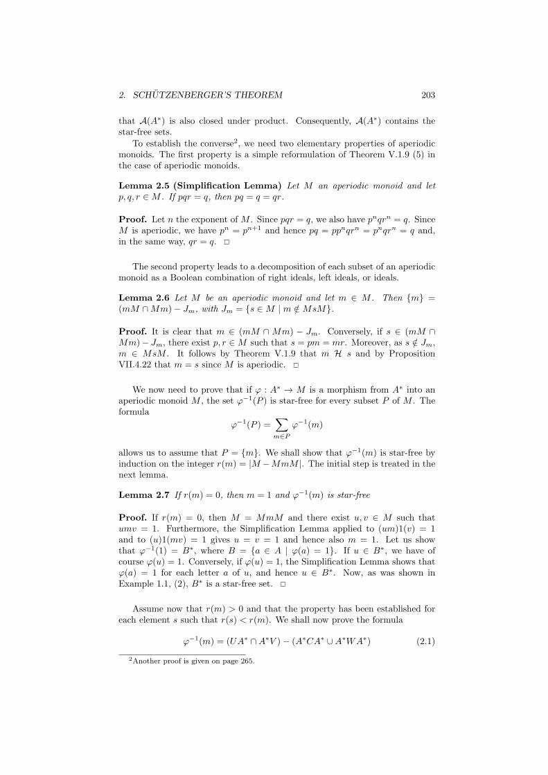
2. SCHUTZENBERGER’S THEOREM 203
that A(A∗) is also closed under product. Consequently, A(A∗) contains thestar-free sets.
To establish the converse2, we need two elementary properties of aperiodicmonoids. The first property is a simple reformulation of Theorem V.1.9 (5) inthe case of aperiodic monoids.
Lemma 2.5 (Simplification Lemma) Let M an aperiodic monoid and letp, q, r ∈M . If pqr = q, then pq = q = qr.
Proof. Let n the exponent of M . Since pqr = q, we also have pnqrn = q. SinceM is aperiodic, we have pn = pn+1 and hence pq = ppnqrn = pnqrn = q and,in the same way, qr = q.
The second property leads to a decomposition of each subset of an aperiodicmonoid as a Boolean combination of right ideals, left ideals, or ideals.
Lemma 2.6 Let M be an aperiodic monoid and let m ∈ M . Then {m} =(mM ∩Mm)− Jm, with Jm = {s ∈M | m /∈MsM}.
Proof. It is clear that m ∈ (mM ∩ Mm) − Jm. Conversely, if s ∈ (mM ∩Mm)− Jm, there exist p, r ∈M such that s = pm = mr. Moreover, as s /∈ Jm,m ∈ MsM . It follows by Theorem V.1.9 that m H s and by PropositionVII.4.22 that m = s since M is aperiodic.
We now need to prove that if ϕ : A∗ → M is a morphism from A∗ into anaperiodic monoid M , the set ϕ−1(P ) is star-free for every subset P of M . Theformula
ϕ−1(P ) =∑
m∈P
ϕ−1(m)
allows us to assume that P = {m}. We shall show that ϕ−1(m) is star-free byinduction on the integer r(m) = |M −MmM |. The initial step is treated in thenext lemma.
Lemma 2.7 If r(m) = 0, then m = 1 and ϕ−1(m) is star-free
Proof. If r(m) = 0, then M = MmM and there exist u, v ∈ M such thatumv = 1. Furthermore, the Simplification Lemma applied to (um)1(v) = 1and to (u)1(mv) = 1 gives u = v = 1 and hence also m = 1. Let us showthat ϕ−1(1) = B∗, where B = {a ∈ A | ϕ(a) = 1}. If u ∈ B∗, we have ofcourse ϕ(u) = 1. Conversely, if ϕ(u) = 1, the Simplification Lemma shows thatϕ(a) = 1 for each letter a of u, and hence u ∈ B∗. Now, as was shown inExample 1.1, (2), B∗ is a star-free set.
Assume now that r(m) > 0 and that the property has been established foreach element s such that r(s) < r(m). We shall now prove the formula
ϕ−1(m) = (UA∗ ∩A∗V )− (A∗CA∗ ∪A∗WA∗) (2.1)
2Another proof is given on page 265.

204 CHAPTER X. STAR-FREE LANGUAGES
where
U =∑
(n,a)∈E
ϕ−1(n)a V =∑
(a,n)∈F
aϕ−1(n)
C = {a ∈ A | m /∈Mϕ(a)M} W =∑
(a,n,b)∈G
aϕ−1(n)b
with
E = {(n, a) ∈M ×A | nϕ(a) R m but n /∈ mM}
F = {(a, n) ∈ A×M | ϕ(a)n L m but n /∈Mm}
G = {(a, n, b) ∈ A×M ×A |
m ∈ (Mϕ(a)nM ∩Mnϕ(b)M)−Mϕ(a)nϕ(b)M}
Denote by L the right-hand side of (2.1). We first prove the inclusion ϕ−1(m) ⊆L. Let u ∈ ϕ−1(m) and let p be the shortest prefix of u such that ϕ(p) R m.The word p cannot be empty, since otherwise m R 1, whence m = 1 by theSimplification Lemma. Put p = ra with r ∈ A∗ and a ∈ A and let n = ϕ(r).By construction, (n, a) ∈ E since
(a) nϕ(a) = ϕ(r)ϕ(a) = ϕ(p) R m,
(b) sincem 6R ϕ(p) = nϕ(a) 6R n, one has n /∈ mM , for otherwise we wouldhave n R m.
It follows that p ∈ ϕ−1(n)a and u ∈ UA∗. A symmetric argument shows thatu ∈ A∗V . If u ∈ A∗CA∗, there exists a letter a of C such that m = ϕ(u) ∈Mϕ(a)M , a contradiction to the definition of C. Similarly, if u ∈ A∗WA∗, thereexist (a, n, b) ∈ G such that m ∈ Mϕ(a)nϕ(b)M , a contradiction this time tothe definition of G. Therefore u ∈ L.
Conversely, let u ∈ L and let s = ϕ(u). Since u ∈ UA∗, we have u ∈ϕ−1(n)aA∗ for some (n, a) ∈ E and hence s = ϕ(u) ∈ nϕ(a)M . Now, since(n, a) ∈ E, nϕ(a)M = mM and thus s ∈ mM . A dual argument shows thatu ∈ V A∗ implies s ∈ Mm. By Lemma 2.6, in order to prove that s = m, andhence that u ∈ ϕ−1(m), it suffices to prove that s /∈ Jm, that is, m ∈ MsM .Supposing the contrary, consider a factor f of u of minimal length such thatm /∈Mϕ(f)M . The word f is necessarily nonempty. If f is a letter, this letteris in C and u ∈ A∗CA∗, which is impossible. We may thus set f = agb, witha, b ∈ A. Set n = ϕ(g). Since f is of minimal length, we have m ∈ Mϕ(a)nMandm ∈Mnϕ(b)M . Consequently (a, n, b) ∈ G and f ∈W , which is impossibleagain.
Formula (2.1) is thus established and it suffices now to show that U , Vand W are star-free, since we have already seen in Example 1.1 that A∗CA∗
is star-free. Let (n, a) ∈ E. Since nϕ(a)M = mM , we have MmM ⊆ MnMand hence r(n) 6 r(m). Moreover, as m 6R n, Theorem V.1.9 shows thatif MmM = MnM , we have n R m, which is not possible since n /∈ mM .Therefore r(n) < r(m) and U is star-free by the induction hypothesis.
A symmetric argument works for V . It remains to treat the case of W .Let (a, n, b) ∈ G. One has r(n) 6 r(m) since m ∈ MnM . Suppose thatMmM = MnM . Then in particular n ∈ MmM and as m ∈ Mϕ(a)nMand m ∈ Mnϕ(b)M , it follows n ∈ Mϕ(a)nM and n ∈ Mnϕ(b)M , whencen L ϕ(a)n and n R nϕ(b). By Proposition V.1.10, nϕ(b) L ϕ(a)nϕ(b), and

2. SCHUTZENBERGER’S THEOREM 205
hence m J ϕ(a)nϕ(b), a contradiction to the definition of G. Consequentlyr(n) < r(m) and W is star-free by the induction hypothesis.
Example 2.1 Let A = {a, b} and let L = (ab)∗. The minimal automaton of Lis represented in Figure 2.1.
1 2
a
b
Figure 2.1. The minimal automaton of (ab)∗.
The syntactic monoid M of L is the monoid consisting of the six matrices
I =
(1 00 1
)a =
(0 10 0
)b =
(0 01 0
)
aa =
(0 00 0
)ab =
(1 00 0
)ba =
(0 00 1
)
and it is defined by the relations a2 = b2 = 0, aba = a and bab = b. Its D-classstructure is given in Figure 2.2:
∗1
∗ab a
b∗ba
∗0
Figure 2.2. The D-class structure of M .
This monoid is aperiodic, since x2 = x3 for each x ∈M , and hence L is star-free.
Example 2.2 Let A = {a, b} and let L′ = (aa)∗. The minimal automaton ofL′ is represented in Figure 2.3:
1 2
a
a
Figure 2.3. The minimal automaton of (aa)∗.
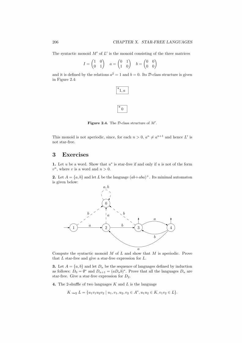
206 CHAPTER X. STAR-FREE LANGUAGES
The syntactic monoid M ′ of L′ is the monoid consisting of the three matrices
I =
(1 00 1
)a =
(0 11 0
)b =
(0 00 0
)
and it is defined by the relations a2 = 1 and b = 0. Its D-class structure is givenin Figure 2.4:
∗1, a
∗0
Figure 2.4. The D-class structure of M ′.
This monoid is not aperiodic, since, for each n > 0, an 6= an+1 and hence L′ isnot star-free.
3 Exercises
1. Let u be a word. Show that u∗ is star-free if and only if u is not of the formvn, where v is a word and n > 0.
2. Let A = {a, b} and let L be the language (ab+aba)+. Its minimal automatonis given below:
0
1 2 3 4a
aa
a
b
b
b
b
a, b
Compute the syntactic monoid M of L and show that M is aperiodic. Provethat L star-free and give a star-free expression for L.
3. Let A = {a, b} and let Dn be the sequence of languages defined by inductionas follows: D0 = ∅∗ and Dn+1 = (aDnb)
∗. Prove that all the languages Dn arestar-free. Give a star-free expression for D2.
4. The 2-shuffle of two languages K and L is the language
K xxy2 L = {u1v1u2v2 | u1, v1, u2, v2 ∈ A∗, u1u2 ∈ K, v1v2 ∈ L}.

4. NOTES 207
(1) Give a rational expression for the language (ab)∗ xxy2 a∗.
(2) Show that the 2-shuffle of two rational languages is rational.
(3) Show that the 2-shuffle of two star-free languages is star-free.
4 Notes
Schutzenberger’s theorem on star-free languages was published in [134]. It isusually considered as the root of algebraic automata theory and it had a con-siderable influence on subsequent research.
Proving that star-free languages are recognized by aperiodic monoids is theeasiest part of the result. In his original proof, Schutzenberger gave a directconstruction to compute a monoid recognising the product of two languages,given two monoids recognising the given languages. This construction, nowa-days called the Schutzenberger product of monoids, is intimately related to theconcatenation product (see [101] for an overview). With this tool in hand, it iseasy to see that the product of two languages recognised by aperiodic monoidsis also recognised by an aperiodic monoid. In this chapter, we followed an-other approach based on relational morphisms, first introduced by Straubing[146, 145]
The most difficult part of Schutzenberger’s theorem consists in establishingthat every language recognised by an aperiodic monoid is star-free. There areessentially two known ways to prove this result. We followed Schutzenberger’soriginal proof, which relies on the properties of Green’s relations. Diekert andKufleitner [38] recently proposed a new proof based on local divisors.
The alternative road, presented in Section XVI.5.3 is a special case of thewreath product principle. This approach was originally proposed by Cohen andBrzozowski [31] and by Meyer [81].

208 CHAPTER X. STAR-FREE LANGUAGES
Chapter XI
Piecewise testable
languages
Simon’s theorem shows that the languages recognised by J -trivial monoids areexactly the shuffle ideals. This result has far reaching consequences, both insemigroup theory and in automata theory.
As a preliminary step, we shall explore the properties of the subword orderingand give an algebraic characterisation of the shuffle ideals.
1 Subword ordering
Let A be a finite alphabet. Recall that a word u = a1 . . . ak ∈ A∗ (wherea1, . . . , ak are letters) is a subword of a word v ∈ A∗ it there exist wordsv0, v1, . . . , vk ∈ A∗ such that v = v0a1v1 · · · akvk. One also says that v is asuperword of u. For instance, ardab is a subword of abracadabra.
The subword ordering is a partial ordering on A∗, which is compatible withthe concatenation product. Here is another important property of the subwordordering, due to Higman:
Theorem 1.1 A set of words of A∗ that are pairwise incomparable for the sub-word ordering is necessarily finite.
Proof. A sequence of words (un)n>0 is said to be subword-free if, for all i < j,ui is not a subword of uj . We claim there exist no infinite subword-free sequence.Otherwise, one would be able to find an “earliest” subword-free sequence, in thefollowing sense:
(1) u0 is a shortest word beginning a subword-free sequence of words,
(2) u1 is a shortest word such that u0, u1 is the beginning of a subword-freesequence of words,
(3) u2 is a shortest word such that u0, u1, u2 is the beginning of a subword-freesequence of words, and so on.
Since A is finite, there exist infinitely many ui that begin with the same letter a,say ui0 = avi0 , ui1 = avi1 , . . . , with i0 < i1 < . . . Let us show that the sequence
u0, u1, . . . , ui0−1, vi0 , vi1 , . . . (1.1)
209
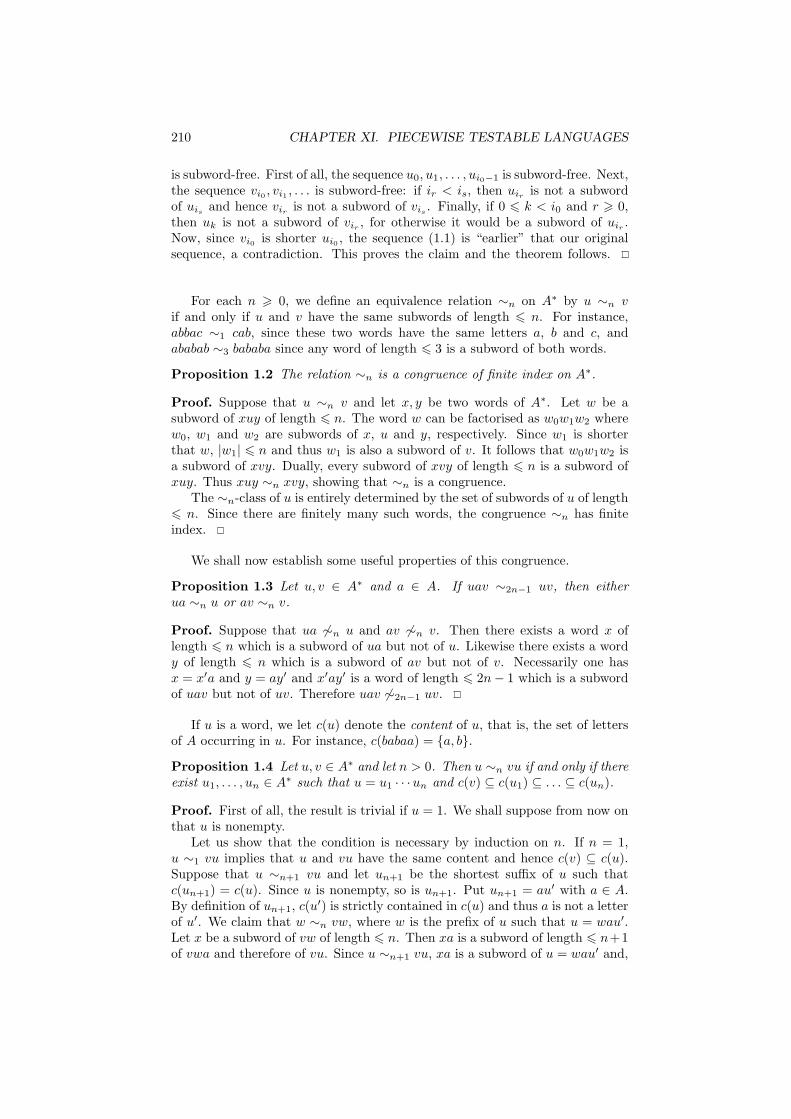
210 CHAPTER XI. PIECEWISE TESTABLE LANGUAGES
is subword-free. First of all, the sequence u0, u1, . . . , ui0−1 is subword-free. Next,the sequence vi0 , vi1 , . . . is subword-free: if ir < is, then uir is not a subwordof uis and hence vir is not a subword of vis . Finally, if 0 6 k < i0 and r > 0,then uk is not a subword of vir , for otherwise it would be a subword of uir .Now, since vi0 is shorter ui0 , the sequence (1.1) is “earlier” that our originalsequence, a contradiction. This proves the claim and the theorem follows.
For each n > 0, we define an equivalence relation ∼n on A∗ by u ∼n vif and only if u and v have the same subwords of length 6 n. For instance,abbac ∼1 cab, since these two words have the same letters a, b and c, andababab ∼3 bababa since any word of length 6 3 is a subword of both words.
Proposition 1.2 The relation ∼n is a congruence of finite index on A∗.
Proof. Suppose that u ∼n v and let x, y be two words of A∗. Let w be asubword of xuy of length 6 n. The word w can be factorised as w0w1w2 wherew0, w1 and w2 are subwords of x, u and y, respectively. Since w1 is shorterthat w, |w1| 6 n and thus w1 is also a subword of v. It follows that w0w1w2 isa subword of xvy. Dually, every subword of xvy of length 6 n is a subword ofxuy. Thus xuy ∼n xvy, showing that ∼n is a congruence.
The ∼n-class of u is entirely determined by the set of subwords of u of length6 n. Since there are finitely many such words, the congruence ∼n has finiteindex.
We shall now establish some useful properties of this congruence.
Proposition 1.3 Let u, v ∈ A∗ and a ∈ A. If uav ∼2n−1 uv, then eitherua ∼n u or av ∼n v.
Proof. Suppose that ua 6∼n u and av 6∼n v. Then there exists a word x oflength 6 n which is a subword of ua but not of u. Likewise there exists a wordy of length 6 n which is a subword of av but not of v. Necessarily one hasx = x′a and y = ay′ and x′ay′ is a word of length 6 2n− 1 which is a subwordof uav but not of uv. Therefore uav 6∼2n−1 uv.
If u is a word, we let c(u) denote the content of u, that is, the set of lettersof A occurring in u. For instance, c(babaa) = {a, b}.
Proposition 1.4 Let u, v ∈ A∗ and let n > 0. Then u ∼n vu if and only if thereexist u1, . . . , un ∈ A∗ such that u = u1 · · ·un and c(v) ⊆ c(u1) ⊆ . . . ⊆ c(un).
Proof. First of all, the result is trivial if u = 1. We shall suppose from now onthat u is nonempty.
Let us show that the condition is necessary by induction on n. If n = 1,u ∼1 vu implies that u and vu have the same content and hence c(v) ⊆ c(u).Suppose that u ∼n+1 vu and let un+1 be the shortest suffix of u such thatc(un+1) = c(u). Since u is nonempty, so is un+1. Put un+1 = au′ with a ∈ A.By definition of un+1, c(u
′) is strictly contained in c(u) and thus a is not a letterof u′. We claim that w ∼n vw, where w is the prefix of u such that u = wau′.Let x be a subword of vw of length 6 n. Then xa is a subword of length 6 n+1of vwa and therefore of vu. Since u ∼n+1 vu, xa is a subword of u = wau′ and,
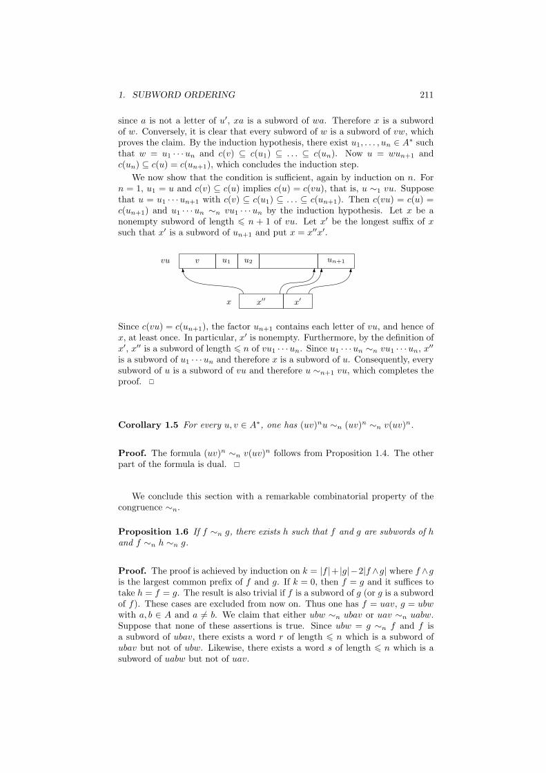
1. SUBWORD ORDERING 211
since a is not a letter of u′, xa is a subword of wa. Therefore x is a subwordof w. Conversely, it is clear that every subword of w is a subword of vw, whichproves the claim. By the induction hypothesis, there exist u1, . . . , un ∈ A
∗ suchthat w = u1 · · ·un and c(v) ⊆ c(u1) ⊆ . . . ⊆ c(un). Now u = wun+1 andc(un) ⊆ c(u) = c(un+1), which concludes the induction step.
We now show that the condition is sufficient, again by induction on n. Forn = 1, u1 = u and c(v) ⊆ c(u) implies c(u) = c(vu), that is, u ∼1 vu. Supposethat u = u1 · · ·un+1 with c(v) ⊆ c(u1) ⊆ . . . ⊆ c(un+1). Then c(vu) = c(u) =c(un+1) and u1 · · ·un ∼n vu1 · · ·un by the induction hypothesis. Let x be anonempty subword of length 6 n + 1 of vu. Let x′ be the longest suffix of xsuch that x′ is a subword of un+1 and put x = x′′x′.
v u1 u2 un+1
x′′ x′
vu
x
Since c(vu) = c(un+1), the factor un+1 contains each letter of vu, and hence ofx, at least once. In particular, x′ is nonempty. Furthermore, by the definition ofx′, x′′ is a subword of length 6 n of vu1 · · ·un. Since u1 · · ·un ∼n vu1 · · ·un, x
′′
is a subword of u1 · · ·un and therefore x is a subword of u. Consequently, everysubword of u is a subword of vu and therefore u ∼n+1 vu, which completes theproof.
Corollary 1.5 For every u, v ∈ A∗, one has (uv)nu ∼n (uv)n ∼n v(uv)n.
Proof. The formula (uv)n ∼n v(uv)n follows from Proposition 1.4. The other
part of the formula is dual.
We conclude this section with a remarkable combinatorial property of thecongruence ∼n.
Proposition 1.6 If f ∼n g, there exists h such that f and g are subwords of hand f ∼n h ∼n g.
Proof. The proof is achieved by induction on k = |f |+ |g|−2|f ∧g| where f ∧gis the largest common prefix of f and g. If k = 0, then f = g and it suffices totake h = f = g. The result is also trivial if f is a subword of g (or g is a subwordof f). These cases are excluded from now on. Thus one has f = uav, g = ubwwith a, b ∈ A and a 6= b. We claim that either ubw ∼n ubav or uav ∼n uabw.Suppose that none of these assertions is true. Since ubw = g ∼n f and f isa subword of ubav, there exists a word r of length 6 n which is a subword ofubav but not of ubw. Likewise, there exists a word s of length 6 n which is asubword of uabw but not of uav.
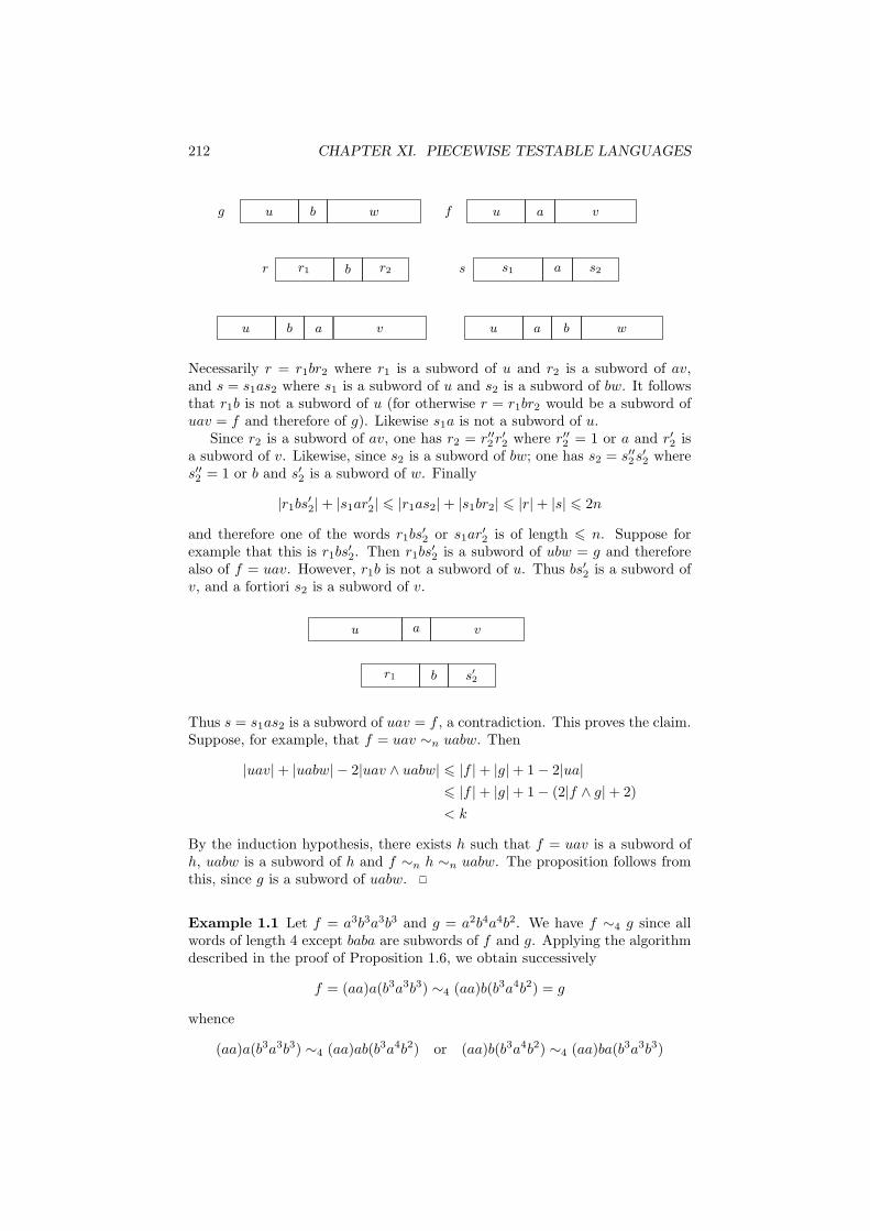
212 CHAPTER XI. PIECEWISE TESTABLE LANGUAGES
g u b w f u a v
r r1 b r2 s s1 a s2
u b a v u a b w
Necessarily r = r1br2 where r1 is a subword of u and r2 is a subword of av,and s = s1as2 where s1 is a subword of u and s2 is a subword of bw. It followsthat r1b is not a subword of u (for otherwise r = r1br2 would be a subword ofuav = f and therefore of g). Likewise s1a is not a subword of u.
Since r2 is a subword of av, one has r2 = r′′2 r′2 where r′′2 = 1 or a and r′2 is
a subword of v. Likewise, since s2 is a subword of bw; one has s2 = s′′2s′2 where
s′′2 = 1 or b and s′2 is a subword of w. Finally
|r1bs′2|+ |s1ar
′2| 6 |r1as2|+ |s1br2| 6 |r|+ |s| 6 2n
and therefore one of the words r1bs′2 or s1ar
′2 is of length 6 n. Suppose for
example that this is r1bs′2. Then r1bs
′2 is a subword of ubw = g and therefore
also of f = uav. However, r1b is not a subword of u. Thus bs′2 is a subword ofv, and a fortiori s2 is a subword of v.
u a v
r1 b s′2
Thus s = s1as2 is a subword of uav = f , a contradiction. This proves the claim.Suppose, for example, that f = uav ∼n uabw. Then
|uav|+ |uabw| − 2|uav ∧ uabw| 6 |f |+ |g|+ 1− 2|ua|
6 |f |+ |g|+ 1− (2|f ∧ g|+ 2)
< k
By the induction hypothesis, there exists h such that f = uav is a subword ofh, uabw is a subword of h and f ∼n h ∼n uabw. The proposition follows fromthis, since g is a subword of uabw.
Example 1.1 Let f = a3b3a3b3 and g = a2b4a4b2. We have f ∼4 g since allwords of length 4 except baba are subwords of f and g. Applying the algorithmdescribed in the proof of Proposition 1.6, we obtain successively
f = (aa)a(b3a3b3) ∼4 (aa)b(b3a4b2) = g
whence
(aa)a(b3a3b3) ∼4 (aa)ab(b3a4b2) or (aa)b(b3a4b2) ∼4 (aa)ba(b3a3b3)

2. SIMPLE LANGUAGES AND SHUFFLE IDEALS 213
The second possibility can be ruled out, for baba is a subword of a2bab3a3b3.Therefore
(a3b3)a(a2b3) ∼4 (a3b3)b(a4b2)
and consequently
(a3b3)a(a2b3) ∼4 (a3b3)ab(a4b2) or (a3b3)b(a4b2) ∼4 (a3b3)ba(a2b3)
The first possibility can be ruled out, for baba is a subword of a3b3aba4b2. Then
(a3b4a3)a(b2) ∼4 (a3b4a3)b(b2)
and consequently
(a3b4a3)a(b2) ∼4 (a3b4a3)ab(b2) or (a3b4a3)b(b2) ∼4 (a3b4a3)ba(b2)
The second possibility can be ruled out, for baba is a subword of a3b4a3bab2.Therefore
a3b4a4b2 ∼4 a3b4a4b3
It follows from this that f and g are subwords of h = a3b4a4b3 and that f ∼4
h ∼4 g.
2 Simple languages and shuffle ideals
The shuffle of two languages L1 and L2 of A∗ is the language L1 xxy L2 of A∗
defined by:
L1 xxy L2 = {w ∈ A∗ | w = u1v1 · · ·unvn for some n > 0 such that
u1 · · ·un ∈ L1, v1 · · · vn ∈ L2}
In particular, if L is a language of A∗, a language of the form L xxy A∗ is calleda shuffle ideal. Thus a language L of A∗ is a shuffle ideal if every superword ofa word of L is also in L.
A simple language is a shuffle ideal of the form
A∗xxy a1 . . . ak = A∗a1A
∗a2A∗ · · ·A∗akA
∗
where a1, . . . , ak ∈ A. Thus A∗a1A
∗a2A∗ · · ·A∗akA
∗ is the set of superwords ofthe word a1 · · · ak. We can now state our first characterisation of shuffle ideals:
Theorem 2.7 A language is a shuffle ideal if and only if it is a finite union ofsimple languages.
Proof. Clearly, every finite union of simple languages is a shuffle ideal. Con-versely, let L be a shuffle ideal and let F be the set of all minimal words ofL for the subword ordering. Thus L is the set of all superwords of F , that isL = F xxy A∗. Furthermore, since the elements of F are pairwise incomparablefor the subword ordering, Higman’s theorem (Theorem 1.1) shows that F isfinite. Therefore L is the finite union of the simple languages A∗ xxy u, wherethe union runs over all words u ∈ F .
214 CHAPTER XI. PIECEWISE TESTABLE LANGUAGES
Corollary 2.8 Every shuffle ideal is a recognisable language.
One can give a constructive proof which does not rely on Higman’s theorem.
Proposition 2.9 Let L be recognisable language such that L xxy A∗ = L. Thenone can effectively find a finite language F such that L = F xxy A∗.
Proof. Let n be the number of states of the minimal automaton A of L. Set
F = {u ∈ L | |u| 6 n} and K = F xxy A∗
We claim that L = K. Since F ⊆ L, one has F xxy A∗ ⊆ L xxy A∗ = L andhence K ⊆ L. If the inclusion is strict, consider a word u of minimal lengthin L −K. Necessarily, |u| > n, for otherwise u ∈ F . Let u = a1 · · · ar and let
q0a1−→ q1 · · · qr−1
ar−→ qr be a successful path with label u inA. As r > n, thereexist two indices i < j such that qi = qj . Thus the word v = a1 · · · aiaj+1 · · · aris also accepted by A and therefore belongs to L. Furthermore, since v is shorterthan u, v belongs to K and u belongs to K xxy A∗. Now, since
K xxy A∗ = (F xxy A∗) xxy A∗ = F xxy (A∗xxy A∗) = F xxy A∗ = K
one has u ∈ K, a contradiction. This proves the claim and the proposition.
We now come to the algebraic characterisation of shuffle ideals.
Theorem 2.10 A language is a shuffle ideal if and only if its ordered syntacticmonoid satisfies the identity 1 6 x.
Proof. Let L be a language and let η : A∗ → (M,6) be its ordered syntacticmorphism. Suppose that L is a shuffle ideal. If uv ∈ L, then uxv ∈ L for eachx ∈ A∗. Therefore 1 6L x and thus M satisfies the identity 1 6 x.
Conversely, if M satisfies the identity 1 6 x, then, for every x ∈ A∗, 1 6L x,that is, the condition uv ∈ L implies uxv ∈ L. Therefore L is a shuffle ideal.
3 Piecewise testable languages and Simon’s the-
orem
A language is called piecewise testable if and only if it is a union of ∼n-classesfor some positive integer n.
The terminology chosen can be explained as follows: a language L is piece-wise testable if there exists an integer n > 0 such that one can test whetheror not a word belongs to L by simple inspection of its subwords of length 6 n.Here is a first description of these languages.
Proposition 3.11 A language of A∗ is piecewise testable if and only if it be-longs to the Boolean algebra generated by the simple languages on A∗.
Proof. Let L = A∗a1A∗ · · · anA
∗ be a simple language of A∗. If u ∈ L, thena1 · · · an is a subword of u. Therefore, if u ∼n v, a1 · · · an is also a subword of vand v ∈ L. This shows that L is saturated by ∼n and therefore is a finite unionof ∼n-classes.

3. PIECEWISE TESTABLE LANGUAGES AND SIMON’S THEOREM 215
Let u be a word of A∗. A moment’s reflection should suffice to verify thefollowing formula:
{v ∈ A∗ | v ∼n u} =( ⋂
a1···ak∈E
A∗a1A∗ · · · akA
∗)−( ⋃
a1···ak∈F
A∗a1A∗ · · · akA
∗)
where E is the set of subwords of u of length 6 n and F is the set of wordsof length 6 n which are not subwords of u. It follows from this formula thatif L is a union of ∼n-classes for some positive integer n, then L belongs to theBoolean algebra generated by the simple languages on A∗.
The syntactic characterisation of piecewise testable languages is the mainresult of this chapter. It relies on two results of semigroup theory that haveindependent interest.
Proposition 3.12 Every finite ordered monoid satisfying the identity 1 6 x isJ -trivial.
Proof. Let x and y be two elements of M such that x J y. Then x = rysand y = uxv for some r, s, u, v ∈ M . Since 1 6 u and 1 6 v, it follows thatx 6 uxv = y and similarly, y 6 x. Thus x = y.
Theorem 3.13 (Simon) Let M be a finite J -trivial monoid and let n be themaximal length of strict <J -chains in M . If ϕ : A∗ → M is a surjectivemorphism, then M is a quotient of the monoid A∗/∼2n−1.
Proof. By Proposition II.3.22, it suffices to show that if f ∼2n−1 g, then ϕ(f) =ϕ(g). By Proposition 1.6, we may assume that f is a subword of g. We notefurthermore that if f is a subword of h and h is a subword of g, then we also havef ∼2n−1 h. This enables us to assume that f = uv and g = uav for some a ∈ A.In this case, Proposition 1.3 shows that either ua ∼n u or av ∼n v. Assumingthe latter, there exists by Proposition 1.4 a factorisation v = v1v2 · · · vn suchthat {a} ⊆ c(v1) ⊆ . . . ⊆ c(vn). Consider the 6J -chain of length n+ 1
ϕ(v1 · · · vn) 6J ϕ(v2 · · · vn) 6J · · · 6J ϕ(vn) 6J 1
By the choice of n, this chain is not strict and there exists an index i suchthat ϕ(vi · · · vn) J ϕ(vi+1 · · · vn). Since M is J -trivial, one has ϕ(vi · · · vn) =ϕ(vi+1 · · · vn) = s. Let b ∈ c(vi). Then vi = v′ibv
′′i for some v′i, v
′′i ∈ A
∗ and thuss = ϕ(vi · · · vn) 6J ϕ(bv′′i vi+1 · · · vn) 6J ϕ(v′′i vi+1 · · · vn) 6J ϕ(vi+1 · · · vn) =s. Since M is J -trivial, we get
s = ϕ(vi · · · vn) = ϕ(bv′′i vi+1 · · · vn) = ϕ(v′′i vi+1 · · · vn) = ϕ(vi+1 · · · vn).
Consequently, one has ϕ(b)s = s for each b ∈ c(vi) and hence also for b ∈ c(vi−1),. . . , b ∈ c(v0) and b = a. Therefore ϕ(v) = ϕ(v1 · · · vn) = s = ϕ(a)s = ϕ(av).It follows that ϕ(f) = ϕ(uav) = ϕ(uv) = ϕ(g), which concludes the proof.
We now return to the announced characterisation of piecewise testable lan-guages.
216 CHAPTER XI. PIECEWISE TESTABLE LANGUAGES
Theorem 3.14 (Simon) A language is piecewise testable if and only if its syn-tactic monoid is finite and J -trivial.
Proof. Let L be a simple language. Then by Theorem 2.10, the ordered syn-tactic monoid of L satisfies the identity 1 6 x. By Proposition 3.12, this monoidis J -trivial. Now if L is piecewise testable, it is by Proposition 3.11 a Booleancombination of simple languages, its syntactic monoid divides a product of finiteJ -trivial monoids and hence is itself finite and J -trivial.
Conversely, if the syntactic monoid of L is finite and J -trivial, then byTheorem 3.13, L is a union of ∼2n−1-classes, where n is the maximal length ofstrict <J -chains in M . Thus L is piecewise testable.
4 Some consequences of Simon’s theorem
Simon’s theorem has unexpected consequences in semigroup theory. We startby defining, for each integer n > 0, three monoids Cn, Rn and Un which willserve us as examples of J -trivial monoids.
The monoid Cn is the submonoid of Tn consisting of all order preserving andextensive functions from {1, . . . , n} into itself. Recall that a transformation aon {1, . . . , n} is order preserving if p 6 q implies p· a 6 q · a and extensive if forall p, p 6 p· a.
The monoid Rn is the monoid of all reflexive relations on {1, . . . , n}. Itis convenient to consider Rn as the monoid of Boolean matrices of size n × nhaving only entries 1 on the diagonal. For example
R2 = {( 1 00 1 ) , (
1 10 1 ) , (
1 01 1 ) , (
1 11 1 )}
Finally, Un is the submonoid of Rn consisting of the upper triangular matricesof Cn. The matrices of Un are called unitriangular. For example,
U3 ={(
1 ε1 ε20 1 ε30 0 1
)| ε1, ε2, ε3 ∈ {0, 1}
}
Proposition 4.15 For each n > 0, the monoids Cn, Rn and Un are J -trivial.
Proof. Let us show that Cn is J -trivial. If f, g ∈ Cn and f J g, then g = afband f = cgd for some a, b, c, d ∈ Cn. Let p ∈ {1, . . . , n}. Since a is extensive,one has p 6 p· a and since f is order-preserving, one has p· f 6 p· af . It follows,since b is extensive, that p· af 6 p· afb and finally p· f 6 p· afb = p· g. Similarreasoning would show that p· g 6 p· f . It follows that f = g and thus Cn isJ -trivial.
Since Un is a submonoid of Rn, it is sufficient to establish that Rn is J -trivial. But Rn is naturally ordered by the order defined by m 6 n if and onlyif, for all i, j, mi,j 6 ni,j and this order is stable under product. Since all entrieson the diagonal are equal to 1, the identity 1 6 x holds in Rn and thus Rn isJ -trivial by Proposition 3.12.
The next proposition gives another property of the monoids Cn, Rn and Un.
Proposition 4.16 For each n,m > 0, the monoid Cn×Cm, [Rn×Rm,Un×Um]is isomorphic to a submonoid of Cn+m [Rn+m,Un+m].

4. SOME CONSEQUENCES OF SIMON’S THEOREM 217
Proof. Let ϕ : Cn × Cm → Cn+m be the function defined by ϕ(f, g) = h where
p·h =
{p· f if 1 6 p 6 n,
(p− n)· g + n if n+ 1 6 p 6 n+m
Then ϕ is clearly an injective morphism and therefore Cn×Cm is isomorphic toa submonoid of Cn+m.
Let now ψ : Rn×Rm → Rn+m be the function defined by ψ(R,S) = T whereT is the relation defined by (i, j) ∈ T if and only if (i, j) ∈ R or (i−n, j−n) ∈ S.Then ψ is an injective morphism and therefore Rn × Rm is isomorphic to asubmonoid of Rn+m. The proof is similar for Un.
The next result shows that the monoids Cn, Rn and Un generate the varietyof J -trivial monoids.
Theorem 4.17 Let M be a finite monoid. The following conditions are equiv-alent:
(1) M is J -trivial,
(2) there exists an integer n > 0 such that M divides Cn,
(3) there exists an integer n > 0 such that M divides Rn,
(4) there exists an integer n > 0 such that M divides Un.
Proof. By Proposition 4.15, the monoids Cn, Rn and Un are J -trivial. There-fore each of the conditions (2), (3) or (4) implies (1). Moreover (4) implies (3)since Un is a submonoid of Rn. It remains to prove that (1) implies (2) and (4).
Let M be a J -trivial monoid. By Proposition VIII.7.20, there exist a finitealphabet A and languages L1, . . . , Lk ∈ J (A
∗) such that M is isomorphic to asubmonoid of M(L1)× · · · ×M(Lk). Now by Theorem 3.14 and by Proposition3.11, each Li is a Boolean combination of simple languages. It follows now fromProposition IV.4.26 that M divides a product of syntactic monoids of simplelanguages. Therefore, by Proposition 4.16, it suffices to establish (2) and (4)when M is the syntactic monoid of a simple language L = A∗a1A
∗ · · · anA∗.
The minimal automaton A of L is pictured in Figure 4.1:
0 1 n− 1 na1 a2 an
A− a1 A− a2 A− an A
. . .
Figure 4.1. An automaton recognising L.
Since the transitions of A are increasing and extensive functions, the transitionmonoid of A, which is also the syntactic monoid of L, is a submonoid of Cn+1,which proves that (1) implies (2).
Furthermore, L is also recognised by the nondeterministic automaton B rep-resented in Figure 4.2:

218 CHAPTER XI. PIECEWISE TESTABLE LANGUAGES
0 1 n− 1 na1 a2 an
A A A A
. . .
Figure 4.2. A nondeterministic automaton recognising L.
The transition monoid of B is a monoid of unitriangular Boolean matrices, thatis, a submonoid of Un+1. It follows that M divides Un+1.
Theorem 3.13 has another very important consequence.
Theorem 4.18 Every finite J -trivial monoid is a quotient of a finite orderedmonoid satisfying the identity 1 6 x.
Proof. Let M be a J -trivial monoid. By Theorem 3.13, M is a quotient ofthe monoid of the form A∗/∼k. Now, the subword ordering induces a stablepartial order on A∗/∼k. Furthermore, since the empty word is a subword ofevery word, the identity 1 6 x holds in this ordered monoid.
5 Exercises
1. Let L = A∗0a1A
∗1 · · · anA
∗n, where a1, . . . , an ∈ A, A0, . . . , An ⊆ A and a1 /∈
A0 ∪A1, a2 /∈ A1 ∪A2, . . . , an /∈ An−1 ∪An. Show that L is piecewise testable.Use this result to show that the language abab∗ca∗b is piecewise testable.
2. Let L be a language. Prove that the following conditions are equivalent:
(1) L is the complement of a shuffle ideal,
(2) L is a finite union of languages of the form A∗0(1 + a1)A
∗1 · · · (1 + an)A
∗n,
where a1, . . . , an ∈ A and A0, . . . , An ⊆ A,
(3) L satisfies the identity x 6 1.
3. Let A be an alphabet. A language L of A∗ is said to be stutter-invariant if,for each letter a ∈ A, a ∼L a
2. The aim of this problem is to study the class Cof all languages that are both stutter-invariant and piecewise testable.
A language of the form
A∗a1A∗a2 · · ·A
∗akA∗
where the ai are letters such that ai 6= ai+1, for 1 6 i 6 k − 1, is said to beelementary stutter-invariant.
(1) Prove that any langage elementary stutter-invariant is stutter-invariant.
(2) Prove that any Boolean combination of elementary stutter-invariant lan-guages belongs to C.
(3) (More difficult) Prove that, conversely, each language of C is a Booleancombination of elementary stutter-invariant languages.
(4) Give a set of profinite equations defining the class C.
6. NOTES 219
6 Notes
We followed Simon’s original proof [137], which is based on a careful analysisof the subword ordering and has a strong combinatorial flavour. Several otherproofs of Simon’s theorem are known. A nice proof via combinatorics on wordswas proposed by Klıma [67]. Straubing and Therien [154] gave a purely algebraicproof by proving directly Theorem 4.18. Another direct proof of 4.18 is due toHenckell and Pin [55]. Almeida [2] proposed an approach using profinite words.
220 CHAPTER XI. PIECEWISE TESTABLE LANGUAGES

Chapter XII
Polynomial closure
The polynomial closure Pol(L) of a class of languages L of A∗ is the set oflanguages that are finite unions of marked products of the form L0a1L1 · · · anLn,where the ai are letters and the Li are elements of L.
The main result of this chapter gives an equational description of Pol(L),given an equational description of L, when L is a lattice of languages closedunder quotient. It can be formally stated as follows:
If L is a lattice of languages closed under quotients, then Pol(L) isdefined by the set of equations of the form xω 6 xωyxω, where x, y areprofinite words such that the equations x = x2 and x 6 y are satisfiedby L.
1 Polynomial closure of a lattice of languages
Let L be a set of languages of A∗. An L-monomial of degree n is a languageof the form L0a1L1 · · · anLn, where each ai is a letter of A and each Li is alanguage of L. An L-polynomial is a finite union of L-monomials. Its degreeis the maximum of the degrees of its monomials. The polynomial closure of L,denoted by Pol(L), is the set of all L-polynomials.
Our main result gives an equational description of Pol(L), given an equa-tional description of L, when L is a lattice of languages closed under quotients.To state this result in a concise way, let us introduce a convenient notation.Given a set R of recognisable languages, let Σ(R) denote the set of equations
of the form xω 6 xωyxω, where x, y are profinite words of A∗ such that theequations x = x2 and x 6 y are satisfied by R. Note that the function mappingR to the class of languages satisfying Σ(R) is monotonic with respect to theinclusion. We can now state our main result:
Theorem 1.1 If L is a lattice of languages closed under quotients, then Pol(L)is defined by the set of equations Σ(L).
The proof is divided into several parts. We first prove in Proposition 1.2that Pol(L) satisfies the equations of Σ(L). To establish the converse of thisproperty, we consider a language K satisfying all the equations of Σ(L). Weconvert this property into a topological property (Proposition 1.3) and thenuse a compactness argument to show that K satisfies the equations of Σ(F),
221

222 CHAPTER XII. POLYNOMIAL CLOSURE
where F is a finite sublattice of L (Proposition 1.4). The final part of the proofconsists in proving that K belongs to Pol(F). This is where the factorisationforest theorem arises, but a series of lemmas (Lemmas 1.5 to 1.10) are stillnecessary to explicitly find a polynomial expression for K.
Proposition 1.2 If L is a lattice of languages, then Pol(L) satisfies the equa-tions of Σ(L).
Proof. Since, by Theorem VIII.2.6, the set of languages satisfying Σ(L) is alattice of languages, it suffices to prove the result for an L-monomial. LetL = L0a1L1 · · · anLn be an L-monomial and let η : A∗ → M be its syntacticmorphism. Let, for 0 6 i 6 n, ηi : A
∗ → Mi be the syntactic morphism of Li.Let x and y be two profinite words such that each Li satisfies the two equationsx = x2 and x 6 y.
Since A∗ is dense in A∗, one can find a word x′ ∈ A∗ such that r(x′, x) >max{|M0|, . . . , |Mn|, |M |}. It follows that η(x′) = η(x) and, for 0 6 i 6 n,ηi(x
′) = ηi(x). Similarly, one can associate with y a word y′ ∈ A∗ such thatη(y′) = η(y) and, for 0 6 i 6 n, ηi(y
′) = ηi(y). It follows that each Li satisfies
the equations x′ = x′2and y′ 6 x′ and that L satisfies the equation xω 6 xωyxω
if and only if it satisfies the equations x′ω6 x′
ωy′x′
ω. In other terms, it suffices
to prove the result when x and y are words.We need to establish the relation
η(xω) 6 η(xωyxω) (1.1)
Let k be an integer such that k > n and η(xω) = η(xk). Since η(xωyxω) =η(xkyxk), proving (1.1) amounts to showing that xk 6L xkyxk. Let u, v ∈ A∗
and suppose that uxkv ∈ L. Thus uxkv = u0a1u1 · · · anun, where, for 0 6i 6 n, ui ∈ Li. Since k > n, one can find h ∈ {0, . . . , n}, j ∈ {1, . . . , k}and u′h, u
′′h ∈ A
∗ such that uh = u′hxu′′h, ux
j−1 = u0a1u1 · · · ahu′h and xk−jv =
u′′hah+1uh+1 · · · anun. Since uh ∈ Lh and Lh satisfies the equations x = x2 andx 6 y, one has u′hx
k−j+1yxju′′h ∈ Lh, and since
uxkyxkv = u0a1u1 · · · ah(u′hx
k−j+1yxju′′h)ah+1uh+1 · · · anun
one gets uxkyxkv ∈ L. Thus xk 6L xkyxk, which completes the proof.
The rest of this section is devoted to showing the converse implication in The-orem 1.1. Let us introduce, for each recognisable language L of A∗, the sets
EL ={(x, y) ∈ A∗ × A∗ | L satisfies x = x2 and x 6 y
}
FL ={(x, y) ∈ A∗ × A∗ | L satisfies xω 6 xωyxω
}.
Lemma VIII.2.7 shows that the set EL is clopen in A∗×A∗. A similar argument,using the continuous map β : A∗ × A∗ →M2 defined by
β(x, y) =(η(xωyxω), η(xω)
)
would show that FL is clopen.We now convert our equational conditions into a topological property. Recall
that a cover [open cover ] of a topological space X is a collection of subsets [opensubsets] of X whose union is X.
1. POLYNOMIAL CLOSURE OF A LATTICE OF LANGUAGES 223
Proposition 1.3 Let F be a set of recognisable languages of A∗ and let K bea recognisable language of A∗. The following conditions are equivalent:
(1) K satisfies the profinite equations of Σ(F),
(2) the set {FK} ∪ {EcL | L ∈ F} is an open cover of A∗ × A∗.
Proof. Indeed F satisfies the two profinite equations x = x2 and x 6 y ifand only if (x, y) ∈
⋂L∈F EL or, equivalently, (x, y) /∈
⋃L∈F E
cL. Similarly, K
satisfies the equation xω 6 xωyxω if and only if (x, y) ∈ FK . Now, condition(1) is equivalent to saying that (x, y) /∈
⋃L∈F E
cL implies (x, y) ∈ FK , which is
another way to say that {FK} ∪ {EcL | L ∈ F} is a cover of A∗ × A∗. Since FK
and EL are clopen, it is an open cover.
Proposition 1.4 If K satisfies the equations of Σ(L), there is a finite subsetF of L such that K satisfies the equations of Σ(F).
Proof. Proposition 1.3 shows that {FK} ∪ {EcL | L ∈ L} is a cover of A∗ × A∗.
Since A∗ is compact, one can extract from this cover a finite cover, say {FK} ∪{Ec
L | L ∈ F}. By Proposition 1.3 again, K satisfies the profinite equationsof the form xω 6 xωyxω such that all the languages of F satisfy the equationsx = x2 and x 6 y.
Let K be a recognisable language satisfying all the equations of Σ(L) andlet η : A∗ → M be its syntactic morphism. Let also F = {L1, . . . , Ln} be afinite subset of L as given by Proposition 1.4. For 1 6 i 6 n, let ηi : A
∗ → Mi
be the syntactic morphism of Li. Let µ : A∗ →M1× · · ·×Mn be the morphism
defined by µ(u) = (η1(u), . . . , ηn(u)). Finally, let V = µ(A∗) and, for 1 6 i 6 n,let πi : V →Mi be the natural projection. We set S = {(η(u), µ(u)) | u ∈ A∗}.Then S is a submonoid of M × V and the two morphisms α : S → M andβ : S → V defined by α(m, v) = m and β(m, v) = v are surjective. Furthermore,the morphism δ : A∗ → S defined by δ(u) = (η(u), µ(u)) satisfies η = α ◦ δ andµ = β ◦ δ. The situation is summarised in the following diagram:
M VS
A∗
Miα β
η µδ
ηi
πi
We now arrive at the last step of the proof of Theorem 1.1, which consists inproving that K belongs to Pol(F).
We start with three auxiliary lemmas. The first one states that every down-ward closed language recognised by µ belongs to L and relies on the fact thatL is a lattice of languages closed under quotients. The second one gives a keyproperty of S and this is the only place in the proof where we use the equationsof Σ(L). The third one is an elementary, but useful, observation.
Lemma 1.5 Let t ∈ V . Then the language µ−1(↑ t) belongs to L.

224 CHAPTER XII. POLYNOMIAL CLOSURE
Proof. Let t = (t1, . . . , tn) and let z be a word such that µ(z) = t. Thenti = ηi(z) and µ−1(↑ t) =
⋂16i6n η
−1i (↑ ti). Moreover, one gets for each i ∈
{1, . . . , n},
η−1i (↑ ti) = {x ∈ A
∗ | ηi(z) 6 ηi(x)} = {x ∈ A∗ | z 6Li
x} =⋂
(u,v)∈Ei
u−1Liv−1
where Ei = {(u, v) ∈ A∗ × A∗ | uzv ∈ Li}. Since Li is recognisable, thereare only finitely many quotients of the form u−1Liv
−1 and hence the intersec-tion is finite. The result follows, since L is a lattice of languages closed underquotients.
Lemma 1.6 For every idempotent (e, f) ∈ S and for every (s, t) ∈ S such thatf 6 t, one has e 6 ese.
Proof. Let x and y be two words such that δ(x) = (e, f) and δ(y) = (s, t).Then η(x) = e, µ(x) = f , η(y) = s and µ(y) = t and since f is idempotent andf 6 t, F satisfies the equations x = x2 and x 6 y. Therefore K satisfies theequation xω 6 xωyxω. It follows that η(xω) 6 η(xωyxω), that is e 6 ese.
Before we continue, let us point out a subtlety in the proof of Lemma 1.6.It looks like we have used words instead of profinite words in this proof andthe reader may wonder whether one could change “profinite” to “finite” in thestatement of our main result. The answer is negative for the following reason: ifF satisfies the equations x = x2 and x 6 y, it does not necessarily imply that Lsatisfies the same equations. In fact, the choice of F comes from the extractionof the finite cover and hence is bound to K.
We now set, for each idempotent f of V , L(f) = µ−1(↑f).
Lemma 1.7 For each idempotent f of V , one has L(1)L(f)L(1) = L(f).
Proof. Since 1 ∈ L(1), one gets the inclusion L(f) = 1L(f)1 ⊆ L(1)L(f)L(1).Let now s, t ∈ L(1) and x ∈ L(f). Then by definition, 1 6 µ(s), f 6 µ(x) and1 6 µ(t). It follows that f = 1f1 6 µ(s)µ(x)µ(t) = µ(sxt), whence sxt ∈ L(f).This gives the opposite inclusion L(1)L(f)L(1) ⊆ L(f).
We now come to the combinatorial argument of the proof. By TheoremII.6.40, there exists a factorisation forest F of height 6 3|S| − 1 which is Ram-seyan modulo δ. We use this fact to associate with each word x a certainlanguage R(x), defined recursively as follows:
R(x) =
L(1)xL(1) if |x| 6 1
R(x1)R(x2) if F (x) = (x1, x2)
R(x1)L(f)R(xk) if F (x) = (x1, . . . , xk), with k > 3 and
δ(x1) = · · · = δ(xk) = (e, f)
In particular R(1) = L(1), since L(1) is a submonoid of A∗. The height functionof F is the function h : A+ → N defined by
h(x) =
{0 if x is a letter
1 + max{h(xi) | 1 6 i 6 k} if F (x) = (x1, . . . , xk)

1. POLYNOMIAL CLOSURE OF A LATTICE OF LANGUAGES 225
Thus h(x) is the length of the longest path with origin in x in the tree of x.Denote by E the finite set of languages of the form L(f), where f is an idem-
potent of V . We know by Lemma 1.5 that E is a subset of L. Let us say that anE-monomial is in normal form if it is of the form L(1)a0L(f1)a1 · · ·L(fk)akL(1)where f1, . . . , fk are idempotents of V .
Lemma 1.8 For each x ∈ A∗, R(x) is equal to an E-monomial in normal formof degree 6 2h(x).
Proof. We prove the result by induction on the length of x. The result is trueif |x| 6 1. Suppose that |x| > 2. If F (x) = (x1, x2), then R(x) = R(x1)R(x2)otherwise R(x) = R(x1)L(f)R(xk). We treat only the latter case, since thefirst one is similar. By the induction hypothesis, R(x1) and R(xk) are equal toE-monomials in normal form. It follows by Lemma 1.7 that R(x) is equal toan E-monomial in normal form, whose degree is lesser than or equal to the sumof the degrees of R(x1) and R(xk). The result now follows from the inductionhypothesis, since 2h(x1) + 2h(xk) 6 21+max{h(x1),...,h(xk)} 6 2h(x).
Lemma 1.9 For each x ∈ A∗, one has x ∈ R(x).
Proof. We prove the result by induction on the length of x. The result istrivial if |x| 6 1. Suppose that |x| > 2. If F (x) = (x1, x2), one has x1 ∈R(x1) and x2 ∈ R(x2) by the induction hypothesis and hence x ∈ R(x) sinceR(x) = R(x1)R(x2). Suppose now that F (x) = (x1, . . . , xk) with k > 3 andδ(x1) = · · · = δ(xk) = (e, f). Then R(x) = R(x1)L(f)R(xk). Since x1 ∈ R(x1)and xk ∈ R(xk) by the induction hypothesis and µ(x2 · · ·xk−1) = f , one getsx2 · · ·xk−1 ∈ L(f) and finally x ∈ R(x1)L(f)R(xk), that is, x ∈ R(x).
If R is a language, let us write η(x) 6 η(R) if, for each u ∈ R, η(x) 6 η(u).
Lemma 1.10 For each x ∈ A∗, one has η(x) 6 η(R(x)).
Proof. We prove the result by induction on the length of x. First, applyingLemma 1.6 with e = f = 1 shows that if (s, t) ∈ S and 1 6 t, then 1 6 s. Itfollows that 1 6 η(µ−1(↑1)) = η(L(1)) = η(R(1)).
If |x| 6 1, one gets R(x) = L(1)xL(1) and η(x) 6 η(L(1))η(x)η(L(1)) =η(R(x)) since 1 6 η(L(1)). Suppose now that |x| > 2. If F (x) = (x1, x2),then R(x) = R(x1)R(x2) and by the induction hypothesis, η(x1) 6 η(R(x1))and η(x2) 6 η(R(x2)). Therefore, η(x) = η(x1)η(x2) 6 η(R(x1))η(R(x2)) =η(R(x)). Finally, suppose that F (x) = (x1, . . . , xk) with k > 3 and δ(x1) =· · · = δ(xk) = (e, f). Then R(x) = R(x1)L(f)R(xk). By the induction hypoth-esis, e 6 η(R(x1)) and e 6 η(R(xk)). Now, if u ∈ L(f), one gets f 6 µ(u). Since(η(u), µ(u)) ∈ S, it follows from Lemma 1.6 that the relation e 6 eη(u)e holdsin M . Finally, we get η(x) = e 6 eη(L(f))e 6 η(R(x1))η(L(f))η(R(xk)) =η(R(x)).
We can now conclude the proof of Theorem 1.1. We claim that K =⋃x∈K R(x). The inclusion K ⊆
⋃x∈K R(x) is an immediate consequence of
Lemma 1.9. To prove the opposite inclusion, consider a word u ∈ R(x) for somex ∈ K. It follows from Lemma 1.10 that η(x) 6 η(u). Since η(x) ∈ η(K), onegets η(u) ∈ η(K) and finally u ∈ K. Now, by Lemma 1.8, each language R(x)

226 CHAPTER XII. POLYNOMIAL CLOSURE
is an E-monomial of degree 6 2h(x). Since h(x) 6 3|S| − 1 for all x, and since Eis finite, there are only finitely many such monomials. Therefore K is equal toan E-polynomial. Finally, Lemma 1.5 shows that each E-polynomial belongs toPol(L), and thus K ∈ Pol(L).
2 A case study
As an application of this result, we establish a set of profinite equations definingthe class of languages of the form L0a1L1 · · · anLn, where each language Li iseither of the form u∗ (where u is a word) or A∗ (where A is the alphabet) andwe prove that this class is decidable.
We have seen that the recognisable languages that are either slender or fullform a lattice of languages closed under quotients, denoted by S in the sequel.One can show that the languages of Pol(S) are finite unions of languages of theform L0a1L1 · · · anLn, where the ai are letters and the Li are languages of theform A∗ or u∗ for some word u. In particular, Pol(S) contains all recognisablesparse languages but it also contains the nonsparse language A∗ if |A| > 2.
An equational description of Pol(S) was given in [16]. Let Σ′(S) denote theset of equations of the form
(xωyω)ω 6 (xωyω)ωz(xωyω)ω
where z ∈ A∗ and x, y ∈ A+ and i(x) 6= i(y).
Theorem 2.11 A recognisable language of A∗ belongs to Pol(S) if and only ifit satisfies the equations of Σ′(S).

Chapter XIII
Relational morphisms
Relational morphisms form a powerful tool in semigroup theory. Althoughthe study of relational morphisms can be reduced in theory to the study ofmorphisms, their systematic use leads to concise proofs of nontrivial results.Furthermore, they provide a natural definition of the Mal’cev product and itsvariants, an important tool for decomposing semigroups into simpler pieces.
1 Relational morphisms
A relational morphism between two semigroups S and T is a relation τ : S → Twhich satisfies
(1) for every s ∈ S, τ(s) 6= ∅,
(2) for every s1, s2 ∈ S, τ(s1)τ(s2) ⊆ τ(s1s2)
For a relational morphism between two monoids S and T , a third condition isrequired
(3) 1 ∈ τ(1)
The graph of a relational morphism τ is the subset R of S × T defined by
R = {(s, t) ∈ S × T | t ∈ τ(s)}
The following result is an immediate consequence of the definition of a relationalmorphism.
Proposition 1.1 The graph of a relational morphism between two semigroups[monoids ] S and T is a subsemigroup [submonoid ] of S × T .
Let us also mention another immediate result.
Proposition 1.2 The composition of two relational morphisms is a relationalmorphism.
Examples of relational morphisms include two standard classes:
(1) morphisms,
(2) inverses of surjective morphisms.
227

228 CHAPTER XIII. RELATIONAL MORPHISMS
Indeed if α : S → T is a surjective morphism, then the relation α−1 : T → Sis a relational morphism. These two classes generate all relational morphisms.More precisely, every relational morphism is the composition of a morphism andthe inverse of a surjective morphism.
Proposition 1.3 Let τ : S → T be a relational morphism and let R be its graph.Then the projections from S × T onto S and T induce morphisms α : R → Sand β : R→ T such that α is surjective and τ = β ◦ α−1.
Proof. The factorisation of τ as β ◦ α−1 is an immediate consequence of thedefinition. The surjectivity of α stems from the fact that, for all s ∈ S, τ(s) isnonempty.
The factorisation τ = β ◦ α−1, pictured in Figure 1.1 is called the canonicalfactorisation of τ .
S T
R ⊆ S × T
α
τ = β ◦ α−1
β
Figure 1.1. The canonical factorisation of a relational morphism.
We shall see that in most cases the properties of τ are tied to those of β (see inparticular Propositions 2.5 and 3.11).
The next result extends Proposition II.3.8 to relational morphisms. Weremind the reader that if τ is a relation from S into T and T ′ is a subset of T ,then τ−1(T ′) = {s ∈ S | τ(s) ∩ T ′ 6= ∅}.
Proposition 1.4 Let τ : S → T be a relational morphism. If S′ is a subsemi-group of S, then τ(S′) is a subsemigroup of T . If T ′ is a subsemigroup of T ,then τ−1(T ′) is a subsemigroup of S.
Proof. Let t1, t2 ∈ τ(S′). Then t1 ∈ τ(s1) and t2 ∈ τ(s2) for some s1, s2 ∈ S′.It follows that t1t2 ∈ τ(s1)τ(s2) ⊆ τ(s1s2) ⊆ τ(S′) and therefore τ(S′) is asubsemigroup of T .
Let s1, s2 ∈ τ−1(T ′). Then by definition there exist t1, t2 ∈ T ′ such thatt1 ∈ τ(s1) and t2 ∈ τ(s2). Thus t1t2 ∈ τ(s1)τ(s2) ⊆ τ(s1s2), whence s1s2 ∈τ−1(t1t2). Therefore s1s2 ∈ τ−1(T ′) and hence τ−1(T ′) is a subsemigroup ofS.
Example 1.1 Let E be the set of all injective partial functions from {1, 2, 3, 4}into itself and let F be the set of all bijections on {1, 2, 3, 4}. Let τ be therelation that associates to each injective function f the set of all possible bijectiveextensions of f . For instance, if f is the partial function defined by f(1) = 3
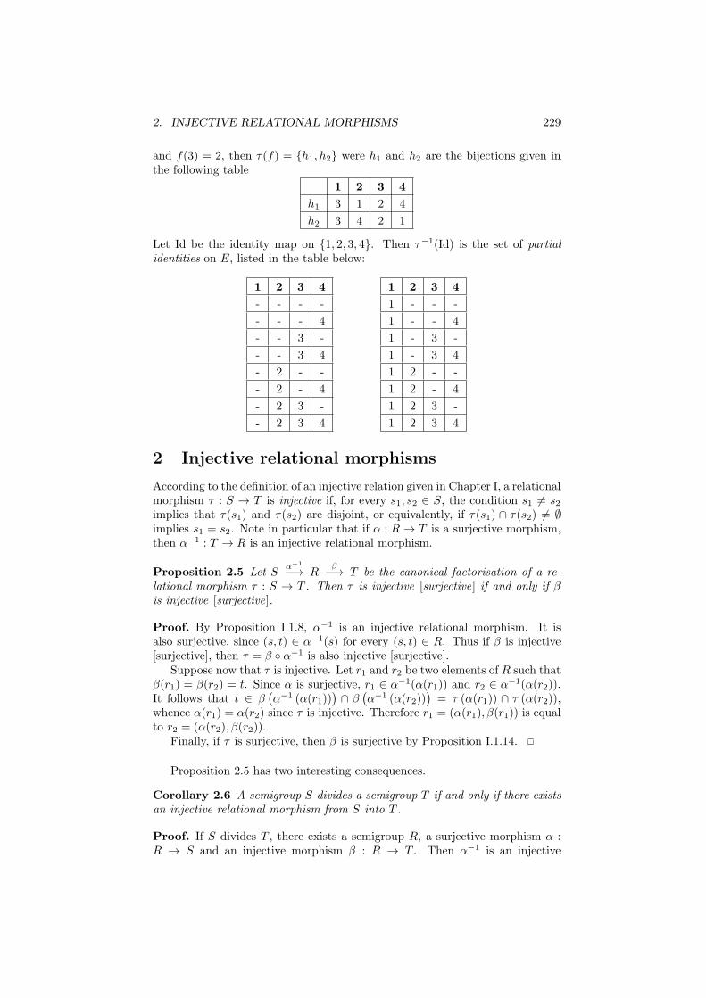
2. INJECTIVE RELATIONAL MORPHISMS 229
and f(3) = 2, then τ(f) = {h1, h2} were h1 and h2 are the bijections given inthe following table
1 2 3 4
h1 3 1 2 4
h2 3 4 2 1
Let Id be the identity map on {1, 2, 3, 4}. Then τ−1(Id) is the set of partialidentities on E, listed in the table below:
1 2 3 4
- - - -
- - - 4
- - 3 -
- - 3 4
- 2 - -
- 2 - 4
- 2 3 -
- 2 3 4
1 2 3 4
1 - - -
1 - - 4
1 - 3 -
1 - 3 4
1 2 - -
1 2 - 4
1 2 3 -
1 2 3 4
2 Injective relational morphisms
According to the definition of an injective relation given in Chapter I, a relationalmorphism τ : S → T is injective if, for every s1, s2 ∈ S, the condition s1 6= s2implies that τ(s1) and τ(s2) are disjoint, or equivalently, if τ(s1) ∩ τ(s2) 6= ∅implies s1 = s2. Note in particular that if α : R→ T is a surjective morphism,then α−1 : T → R is an injective relational morphism.
Proposition 2.5 Let Sα−1
−→ Rβ−→ T be the canonical factorisation of a re-
lational morphism τ : S → T . Then τ is injective [surjective] if and only if βis injective [surjective].
Proof. By Proposition I.1.8, α−1 is an injective relational morphism. It isalso surjective, since (s, t) ∈ α−1(s) for every (s, t) ∈ R. Thus if β is injective[surjective], then τ = β ◦ α−1 is also injective [surjective].
Suppose now that τ is injective. Let r1 and r2 be two elements of R such thatβ(r1) = β(r2) = t. Since α is surjective, r1 ∈ α
−1(α(r1)) and r2 ∈ α−1(α(r2)).
It follows that t ∈ β(α−1 (α(r1))
)∩ β
(α−1 (α(r2))
)= τ (α(r1)) ∩ τ (α(r2)),
whence α(r1) = α(r2) since τ is injective. Therefore r1 = (α(r1), β(r1)) is equalto r2 = (α(r2), β(r2)).
Finally, if τ is surjective, then β is surjective by Proposition I.1.14.
Proposition 2.5 has two interesting consequences.
Corollary 2.6 A semigroup S divides a semigroup T if and only if there existsan injective relational morphism from S into T .
Proof. If S divides T , there exists a semigroup R, a surjective morphism α :R → S and an injective morphism β : R → T . Then α−1 is an injective

230 CHAPTER XIII. RELATIONAL MORPHISMS
relational morphism and thus τ = β ◦ α−1 is an injective relational morphismfrom S into T .
Conversely, if τ is an injective relational morphism from S into T and if
Sα−1
−→ Rβ−→ T is the canonical factorisation of τ . Proposition 2.5 shows that
β is injective. Since α is surjective, S divides T .
Corollary 2.7 Let τ : S → T be an injective relational morphism. Then forany subsemigroup T ′ of T , τ−1(T ′) divides T ′. Furthermore τ−1(E(T )) ⊆ E(S).
Proof. Let Sα−1
−→ Rβ−→ T be the canonical factorisation of τ . Then β is
injective by Proposition 2.5 and thus β−1(T ′) is isomorphic to a subsemigroupof T ′. Finally, τ−1(T ′) is equal to α(β−1(T ′)) and thus divides T ′.
Let s ∈ τ−1(E(T )). Then τ(s) contains some idempotent f of T . Asτ(s)τ(s) ⊆ τ(s2), τ(s2) also contains f . Thus f ∈ τ(s) ∩ τ(s2) whence s = s2
since τ is injective. Thus s is idempotent and τ−1(E(T )) ⊆ E(S).
If T is finite, Corollary 2.7 can be improved as follows.
Proposition 2.8 Let T be a finite semigroup and let τ : S → T be an injectiverelational morphism. Then τ−1(E(T )) = E(S).
Proof. Let e ∈ E(S). By Proposition 1.4, τ(e) is a subsemigroup of T , which,by Corollary II.6.32, contains an idempotent. Thus e ∈ τ−1(E(T )), showingthat E(S) ⊆ τ−1(E(T )). The opposite inclusion follows from Corollary 2.7.
3 Relational V-morphisms
Let V be a variety of finite semigroups. A [relational] morphism τ : S → T issaid to be a [relational ] V-morphism if, for every subsemigroup T ′ of T whichbelongs to V, the semigroup τ−1(T ′) also belongs to V.
The definition can be readily adapted to the case of varieties of orderedsemigroups. Let V be a variety of finite ordered semigroups and let S and Tbe two ordered semigroups. Then a [relational] morphism τ : S → T is said tobe a [relational] V-morphism if, for every ordered subsemigroup T ′ of T whichbelongs to V, the ordered semigroup τ−1(T ′) also belongs to V.
In practice, V is often one of the following varieties:
(1) A, the variety of aperiodic semigroups,
(2) N, the variety of nilpotent semigroups,
(3) L1 = Jese = eK, the variety of locally trivial semigroups,
(4) LJ− = Je 6 eseK, the variety of ordered semigroups S, such that, for alle ∈ E(S), the ordered submonoid eSe satisfies the identity 1 6 x.
A relational A-morphism is also called an aperiodic relational morphism and arelational L1-morphism is also called a locally trivial relational morphism.
The definition of a relational V-morphism is formally reminiscent of that ofa continuous function. This analogy is confirmed by the following proposition,whose proof is immediate.
Proposition 3.9 Relational V-morphisms are closed under composition.

3. RELATIONAL V-MORPHISMS 231
Let us mention another elementary result.
Proposition 3.10 Injective relational morphisms are relational V-morphismsfor every variety V.
Proof. This follows directly from Corollary 2.7.
Note that the converse to Proposition 3.10 does not hold. Let N2 = {0, a}and N3 = {0, a, b} be the nilpotent semigroups with two and three elements,respectively and let ϕ : N3 → N2 be the morphism defined by ϕ(a) = ϕ(b) = aand ϕ(0) = 0. Then the only subsemigroups of N2 are 0 and N2. It followsthat ϕ is a relational V-morphism for every variety V since ϕ−1(0) = 0 andϕ−1(N2) = N3, which divides N2 ×N2. However, ϕ is not injective.
We can now state our announced result on canonical factorisations.
Proposition 3.11 Let Sα−1
−→ Rβ−→ T be the canonical factorisation of a re-
lational morphism τ : S → T . Then τ is a relational V-morphism if and onlyif β is a V-morphism.
Proof. First, α−1 is an injective relational morphism and thus a relational V-morphism by Proposition 3.10. Thus if β is a relational V-morphism, then τ isa relational V-morphism by Proposition 3.9.
Conversely, suppose that τ is a relational V-morphism. Let γ : S × T →T × T be the relational morphism defined by γ(s, t) = τ(s) × {t}. Let T ′ be asubsemigroup of T belonging to V. Setting D = {(t, t) | t ∈ T ′}, one gets
γ−1(D) = {(s, t) ∈ S × T | t ∈ τ(s) ∩ T ′} = β−1(T ′)
It follows that β−1(T ′) is a subsemigroup of τ−1(T ′) × T ′ and thus is in V.Thus β is a relational V-morphism.
Relational morphisms can be restricted to subsemigroups.
Proposition 3.12 Let τ : S → T be a relational morphism and let T ′ be asubsemigroup of T . Then the relation τ : τ−1(T ′) → T ′, defined by τ(s) =τ(s) ∩ T ′, is a relational morphism. Furthermore, if τ is injective [a relationalV-morphism], so is τ .
Proof. Let s ∈ τ−1(T ′). Then by definition τ(s) ∩ T ′ 6= ∅ and thus τ(s) 6= ∅.Let s1, s2 ∈ τ
−1(T ′). One gets
τ(s1)τ(s2) = (τ(s1) ∩ T′)(τ(s2) ∩ T
′)
⊆ τ(s1)τ(s2) ∩ T′ ⊆ τ(s1s2) ∩ T
′ ⊆ τ(s1s2)
and thus τ is a relational morphism. The second part of the statement isobvious.
We now turn to more specific properties of relational V-morphisms.
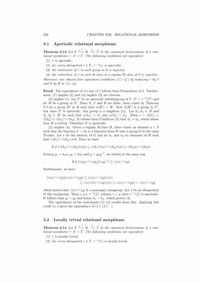
232 CHAPTER XIII. RELATIONAL MORPHISMS
3.1 Aperiodic relational morphisms
Theorem 3.13 Let Sα−1
−→ Rβ−→ T be the canonical factorisation of a rela-
tional morphism τ : S → T . The following conditions are equivalent:
(1) τ is aperiodic,
(2) for every idempotent e ∈ T , τ−1(e) is aperiodic,
(3) the restriction of τ to each group in S is injective,
(4) the restriction of τ to each H-class in a regular D-class of S is injective.
Moreover, one obtains four equivalent conditions (1’)–(4’) by replacing τ by βand S by R in (1)–(4).
Proof. The equivalence of (1) and (1’) follows from Proposition 3.11. Further-more, (1) implies (2) and (4) implies (3) are obvious.
(3) implies (1). Let T ′ be an aperiodic subsemigroup of T , S′ = τ−1(T ′) andlet H be a group in S′. Since S, T and R are finite, there exists by TheoremV.5.45 a group H ′ in R such that α(H ′) = H. Now β(H ′) is a group in T ′,but since T ′ is aperiodic, this group is a singleton {e}. Let h1, h2 ∈ H andh′1, h
′2 ∈ H ′ be such that α(h1) = h′1 and α(h′2) = h2. Then e = β(h′1) =
β(h′2) ∈ τ(h1)∩ τ(h2). It follows from Condition (3) that h1 = h2, which showsthat H is trivial. Therefore S′ is aperiodic.
(2) implies (4). Given a regular H-class H, there exists an element a ∈ Ssuch that the function h→ ha is a bijection from H onto a group G in the sameD-class. Let e be the identity of G and let h1 and h2 be elements of H suchthat τ(h1) ∩ τ(h2) 6= ∅. Then we have
∅ 6= (τ(h1) ∩ τ(h2))τ(a) ⊆ τ(h1)τ(a) ∩ τ(h2)τ(a) ⊆ τ(h1a) ∩ τ(h2a)
Setting g1 = h1a, g2 = h2a and g = g2g−11 , we obtain in the same way
∅ 6= (τ(g1) ∩ τ(g2))τ(g−11 ) ⊆ τ(e) ∩ τ(g)
Furthermore, we have
(τ(e) ∩ τ(g))(τ(e) ∩ τ(g)) ⊆ (τ(e) ∩ τ(g))τ(e)
⊆ τ(e)τ(e) ∩ τ(g)τ(e) ⊆ τ(ee) ∩ τ(ge) = τ(e) ∩ τ(g)
which proves that τ(e)∩τ(g) is a nonempty semigroup. Let f be an idempotentof this semigroup. Then e, g ∈ τ−1(f), whence e = g since τ−1(f) is aperiodic.It follows that g1 = g2 and hence h1 = h2, which proves (4).
The equivalence of the statements (1)–(4) results from this. Applying thisresult to β gives the equivalence of (1’)–(4’).
3.2 Locally trivial relational morphisms
Theorem 3.14 Let Sα−1
−→ Rβ−→ T be the canonical factorisation of a rela-
tional morphism τ : S → T . The following conditions are equivalent:
(1) τ is locally trivial,
(2) for every idempotent e ∈ T , τ−1(e) is locally trivial,
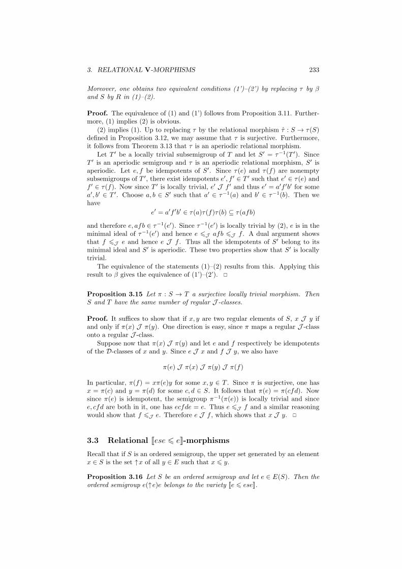
3. RELATIONAL V-MORPHISMS 233
Moreover, one obtains two equivalent conditions (1’)–(2’) by replacing τ by βand S by R in (1)–(2).
Proof. The equivalence of (1) and (1’) follows from Proposition 3.11. Further-more, (1) implies (2) is obvious.
(2) implies (1). Up to replacing τ by the relational morphism τ : S → τ(S)defined in Proposition 3.12, we may assume that τ is surjective. Furthermore,it follows from Theorem 3.13 that τ is an aperiodic relational morphism.
Let T ′ be a locally trivial subsemigroup of T and let S′ = τ−1(T ′). SinceT ′ is an aperiodic semigroup and τ is an aperiodic relational morphism, S′ isaperiodic. Let e, f be idempotents of S′. Since τ(e) and τ(f) are nonemptysubsemigroups of T ′, there exist idempotents e′, f ′ ∈ T ′ such that e′ ∈ τ(e) andf ′ ∈ τ(f). Now since T ′ is locally trivial, e′ J f ′ and thus e′ = a′f ′b′ for somea′, b′ ∈ T ′. Choose a, b ∈ S′ such that a′ ∈ τ−1(a) and b′ ∈ τ−1(b). Then wehave
e′ = a′f ′b′ ∈ τ(a)τ(f)τ(b) ⊆ τ(afb)
and therefore e, afb ∈ τ−1(e′). Since τ−1(e′) is locally trivial by (2), e is in theminimal ideal of τ−1(e′) and hence e 6J afb 6J f . A dual argument showsthat f 6J e and hence e J f . Thus all the idempotents of S′ belong to itsminimal ideal and S′ is aperiodic. These two properties show that S′ is locallytrivial.
The equivalence of the statements (1)–(2) results from this. Applying thisresult to β gives the equivalence of (1’)–(2’).
Proposition 3.15 Let π : S → T a surjective locally trivial morphism. ThenS and T have the same number of regular J -classes.
Proof. It suffices to show that if x, y are two regular elements of S, x J y ifand only if π(x) J π(y). One direction is easy, since π maps a regular J -classonto a regular J -class.
Suppose now that π(x) J π(y) and let e and f respectively be idempotentsof the D-classes of x and y. Since e J x and f J y, we also have
π(e) J π(x) J π(y) J π(f)
In particular, π(f) = xπ(e)y for some x, y ∈ T . Since π is surjective, one hasx = π(c) and y = π(d) for some c, d ∈ S. It follows that π(e) = π(cfd). Nowsince π(e) is idempotent, the semigroup π−1(π(e)) is locally trivial and sincee, cfd are both in it, one has ecfde = e. Thus e 6J f and a similar reasoningwould show that f 6J e. Therefore e J f , which shows that x J y.
3.3 Relational Jese 6 eK-morphisms
Recall that if S is an ordered semigroup, the upper set generated by an elementx ∈ S is the set ↑x of all y ∈ E such that x 6 y.
Proposition 3.16 Let S be an ordered semigroup and let e ∈ E(S). Then theordered semigroup e(↑e)e belongs to the variety Je 6 eseK.
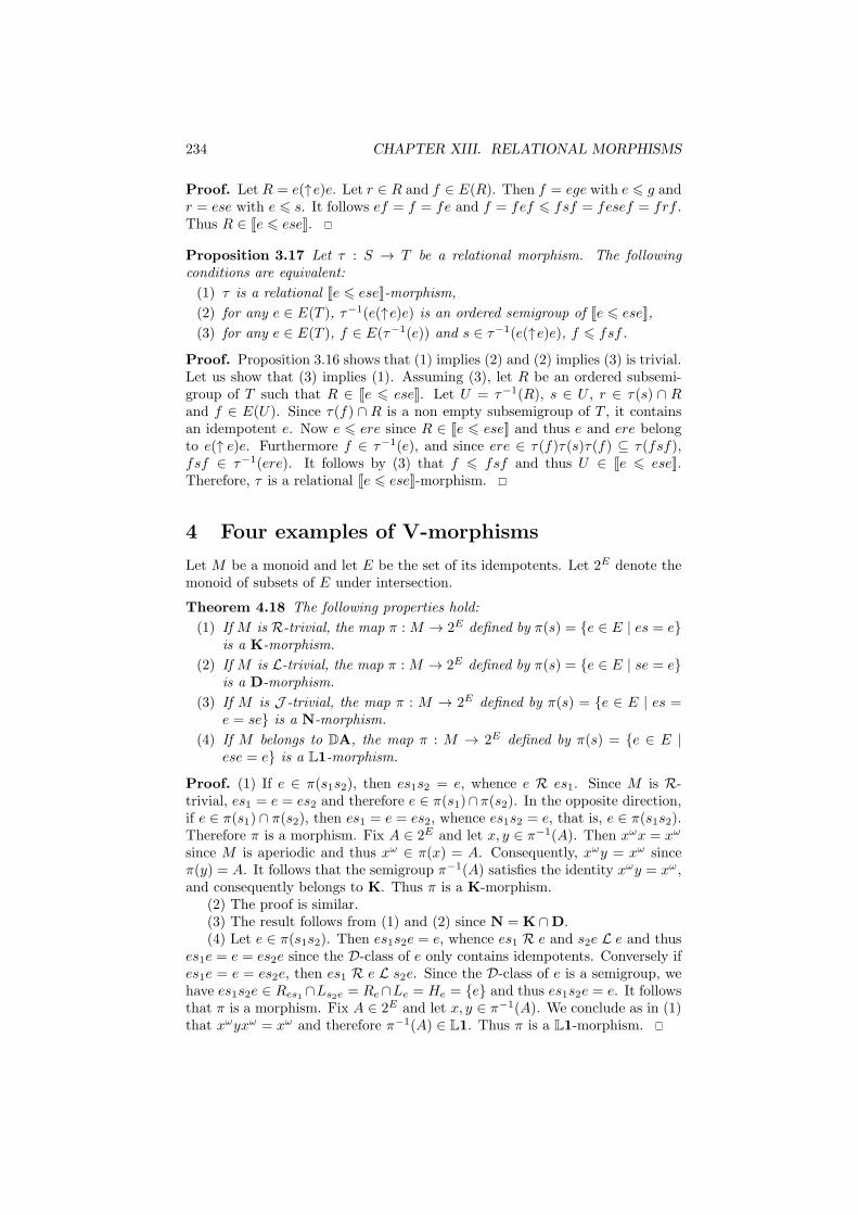
234 CHAPTER XIII. RELATIONAL MORPHISMS
Proof. Let R = e(↑e)e. Let r ∈ R and f ∈ E(R). Then f = ege with e 6 g andr = ese with e 6 s. It follows ef = f = fe and f = fef 6 fsf = fesef = frf .Thus R ∈ Je 6 eseK.
Proposition 3.17 Let τ : S → T be a relational morphism. The followingconditions are equivalent:
(1) τ is a relational Je 6 eseK-morphism,
(2) for any e ∈ E(T ), τ−1(e(↑e)e) is an ordered semigroup of Je 6 eseK,
(3) for any e ∈ E(T ), f ∈ E(τ−1(e)) and s ∈ τ−1(e(↑e)e), f 6 fsf .
Proof. Proposition 3.16 shows that (1) implies (2) and (2) implies (3) is trivial.Let us show that (3) implies (1). Assuming (3), let R be an ordered subsemi-group of T such that R ∈ Je 6 eseK. Let U = τ−1(R), s ∈ U , r ∈ τ(s) ∩ Rand f ∈ E(U). Since τ(f) ∩ R is a non empty subsemigroup of T , it containsan idempotent e. Now e 6 ere since R ∈ Je 6 eseK and thus e and ere belongto e(↑ e)e. Furthermore f ∈ τ−1(e), and since ere ∈ τ(f)τ(s)τ(f) ⊆ τ(fsf),fsf ∈ τ−1(ere). It follows by (3) that f 6 fsf and thus U ∈ Je 6 eseK.Therefore, τ is a relational Je 6 eseK-morphism.
4 Four examples of V-morphisms
Let M be a monoid and let E be the set of its idempotents. Let 2E denote themonoid of subsets of E under intersection.
Theorem 4.18 The following properties hold:
(1) If M is R-trivial, the map π :M → 2E defined by π(s) = {e ∈ E | es = e}is a K-morphism.
(2) If M is L-trivial, the map π :M → 2E defined by π(s) = {e ∈ E | se = e}is a D-morphism.
(3) If M is J -trivial, the map π : M → 2E defined by π(s) = {e ∈ E | es =e = se} is a N-morphism.
(4) If M belongs to DA, the map π : M → 2E defined by π(s) = {e ∈ E |ese = e} is a L1-morphism.
Proof. (1) If e ∈ π(s1s2), then es1s2 = e, whence e R es1. Since M is R-trivial, es1 = e = es2 and therefore e ∈ π(s1)∩π(s2). In the opposite direction,if e ∈ π(s1) ∩ π(s2), then es1 = e = es2, whence es1s2 = e, that is, e ∈ π(s1s2).Therefore π is a morphism. Fix A ∈ 2E and let x, y ∈ π−1(A). Then xωx = xω
since M is aperiodic and thus xω ∈ π(x) = A. Consequently, xωy = xω sinceπ(y) = A. It follows that the semigroup π−1(A) satisfies the identity xωy = xω,and consequently belongs to K. Thus π is a K-morphism.
(2) The proof is similar.(3) The result follows from (1) and (2) since N = K ∩D.(4) Let e ∈ π(s1s2). Then es1s2e = e, whence es1 R e and s2e L e and thus
es1e = e = es2e since the D-class of e only contains idempotents. Conversely ifes1e = e = es2e, then es1 R e L s2e. Since the D-class of e is a semigroup, wehave es1s2e ∈ Res1 ∩Ls2e = Re∩Le = He = {e} and thus es1s2e = e. It followsthat π is a morphism. Fix A ∈ 2E and let x, y ∈ π−1(A). We conclude as in (1)that xωyxω = xω and therefore π−1(A) ∈ L1. Thus π is a L1-morphism.
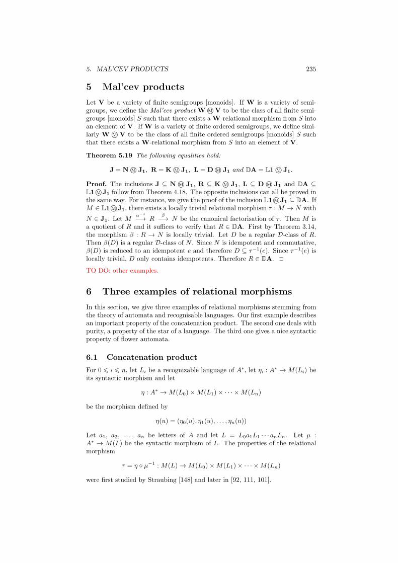
5. MAL’CEV PRODUCTS 235
5 Mal’cev products
Let V be a variety of finite semigroups [monoids]. If W is a variety of semi-groups, we define the Mal’cev product W M©V to be the class of all finite semi-groups [monoids] S such that there exists a W-relational morphism from S intoan element of V. If W is a variety of finite ordered semigroups, we define simi-larly W M©V to be the class of all finite ordered semigroups [monoids] S suchthat there exists a W-relational morphism from S into an element of V.
Theorem 5.19 The following equalities hold:
J = N M© J1, R = K M© J1, L = D M© J1 and DA = L1 M© J1.
Proof. The inclusions J ⊆ N M© J1, R ⊆ K M© J1, L ⊆ D M© J1 and DA ⊆L1 M©J1 follow from Theorem 4.18. The opposite inclusions can all be proved inthe same way. For instance, we give the proof of the inclusion L1 M©J1 ⊆ DA. IfM ∈ L1 M©J1, there exists a locally trivial relational morphism τ :M → N with
N ∈ J1. Let Mα−1
−→ Rβ−→ N be the canonical factorisation of τ . Then M is
a quotient of R and it suffices to verify that R ∈ DA. First by Theorem 3.14,the morphism β : R → N is locally trivial. Let D be a regular D-class of R.Then β(D) is a regular D-class of N . Since N is idempotent and commutative,β(D) is reduced to an idempotent e and therefore D ⊆ τ−1(e). Since τ−1(e) islocally trivial, D only contains idempotents. Therefore R ∈ DA.
TO DO: other examples.
6 Three examples of relational morphisms
In this section, we give three examples of relational morphisms stemming fromthe theory of automata and recognisable languages. Our first example describesan important property of the concatenation product. The second one deals withpurity, a property of the star of a language. The third one gives a nice syntacticproperty of flower automata.
6.1 Concatenation product
For 0 6 i 6 n, let Li be a recognizable language of A∗, let ηi : A∗ →M(Li) be
its syntactic morphism and let
η : A∗ →M(L0)×M(L1)× · · · ×M(Ln)
be the morphism defined by
η(u) = (η0(u), η1(u), . . . , ηn(u))
Let a1, a2, . . . , an be letters of A and let L = L0a1L1 · · · anLn. Let µ :A∗ → M(L) be the syntactic morphism of L. The properties of the relationalmorphism
τ = η ◦ µ−1 :M(L)→M(L0)×M(L1)× · · · ×M(Ln)
were first studied by Straubing [148] and later in [92, 111, 101].
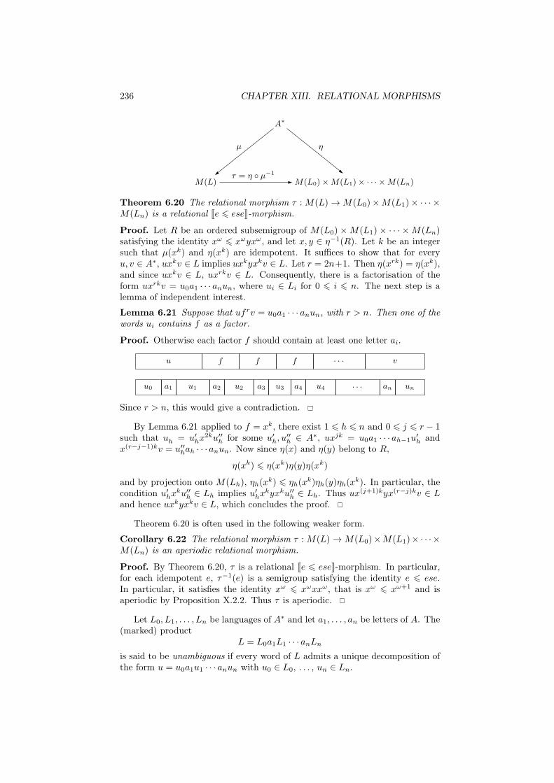
236 CHAPTER XIII. RELATIONAL MORPHISMS
M(L) M(L0)×M(L1)× · · · ×M(Ln)
A∗
µ
τ = η ◦ µ−1
η
Theorem 6.20 The relational morphism τ :M(L)→M(L0)×M(L1)× · · · ×M(Ln) is a relational Je 6 eseK-morphism.
Proof. Let R be an ordered subsemigroup of M(L0) ×M(L1) × · · · ×M(Ln)satisfying the identity xω 6 xωyxω, and let x, y ∈ η−1(R). Let k be an integersuch that µ(xk) and η(xk) are idempotent. It suffices to show that for everyu, v ∈ A∗, uxkv ∈ L implies uxkyxkv ∈ L. Let r = 2n+1. Then η(xrk) = η(xk),and since uxkv ∈ L, uxrkv ∈ L. Consequently, there is a factorisation of theform uxrkv = u0a1 · · · anun, where ui ∈ Li for 0 6 i 6 n. The next step is alemma of independent interest.
Lemma 6.21 Suppose that ufrv = u0a1 · · · anun, with r > n. Then one of thewords ui contains f as a factor.
Proof. Otherwise each factor f should contain at least one letter ai.
u f f f · · · v
u0 a1 u1 a2 u2 a3 u3 a4 u4 · · · an un
Since r > n, this would give a contradiction.
By Lemma 6.21 applied to f = xk, there exist 1 6 h 6 n and 0 6 j 6 r − 1such that uh = u′hx
2ku′′h for some u′h, u′′h ∈ A∗, uxjk = u0a1 · · · ah−1u
′h and
x(r−j−1)kv = u′′hah · · · anun. Now since η(x) and η(y) belong to R,
η(xk) 6 η(xk)η(y)η(xk)
and by projection onto M(Lh), ηh(xk) 6 ηh(x
k)ηh(y)ηh(xk). In particular, the
condition u′hxku′′h ∈ Lh implies u′hx
kyxku′′h ∈ Lh. Thus ux(j+1)kyx(r−j)kv ∈ Land hence uxkyxkv ∈ L, which concludes the proof.
Theorem 6.20 is often used in the following weaker form.
Corollary 6.22 The relational morphism τ :M(L)→M(L0)×M(L1)× · · · ×M(Ln) is an aperiodic relational morphism.
Proof. By Theorem 6.20, τ is a relational Je 6 eseK-morphism. In particular,for each idempotent e, τ−1(e) is a semigroup satisfying the identity e 6 ese.In particular, it satisfies the identity xω 6 xωxxω, that is xω 6 xω+1 and isaperiodic by Proposition X.2.2. Thus τ is aperiodic.
Let L0, L1, . . . , Ln be languages of A∗ and let a1, . . . , an be letters of A. The(marked) product
L = L0a1L1 · · · anLn
is said to be unambiguous if every word of L admits a unique decomposition ofthe form u = u0a1u1 · · · anun with u0 ∈ L0, . . . , un ∈ Ln.

6. THREE EXAMPLES OF RELATIONAL MORPHISMS 237
Example 6.1 Let A = {a, b, c}. The marked product {a, c}∗a{1}b{b, c}∗ isunambiguous.
Theorem 6.23 If the product L0a1L1 · · · anLn is unambiguous, the relationalmorphism τ :M(L)→M(L0)×M(L1)×· · ·×M(Ln) is a locally trivial relationalmorphism.
Proof. By Theorem 3.14, it suffices to show that if e is an idempotent ofM(L0)×M(L1)× · · · ×M(Ln), then the semigroup τ−1(e) is locally trivial. Itfollows from Theorem 6.20 that τ−1(e) satisfies the identity xω 6 xωyxω andit just remains to prove the opposite identity xωyxω 6 xω. Let x, y ∈ η−1(e),let k be an integer such that µ(xk) is idempotent and let h = xk. It suffices toshow that uhyhv ∈ L implies uhv ∈ L. Let r = n+ 2. Then η(hr) = η(h), andif uhyhv ∈ L, then uhryhrv ∈ L. Consequently, there is a factorisation of theform uhryhrv = u0a1 · · · anun, where ui ∈ Li for 0 6 i 6 n.
uhryhrv
u0 a1 u1 a2 u2 · · · an un
First assume that one of the words ui contains hyh as a factor, that is, ui =u′ihyhu
′′i with u0a1 · · · aiu
′i = uhr−1 and u′′i ai+1 · · · anun = hr−1v. Since η(x) =
η(y) = e, one has ηi(hyh) = ηi(h) and hence, u′ihyhu′′i ∈ Li implies u′ihu
′′i ∈ Li.
Consequently, one has
uh2r−1v = uhr−1hhr−1v = u0a1 · · · ai(u′ihu
′′i )ai+1 · · · anun
which shows that uh2r−1v belongs to L. Since η(h2r−1) = η(h), it follows thatuhv is also in L, as required.
Suppose now that none of the words ui contains hyh as a factor. Then thereare factorisations of the form
uhr−1 = u0a1 · · · aiu′i hyh = u′′i ai+1 · · · aju
′j hr−1v = u′′j aj+1 · · · anun
with ui = u′iu′′i and uj = u′ju
′′j . By Lemma 6.21 applied to the word u0a1 · · · aiu
′i,
one of the words u0, . . . , ui−1, u′i contains h as a factor. Similarly, one of the
words u′′j , uj+1, . . . , un contains h as a factor. Therefore one gets factorisations
uhr−1 = u0a1 · · · aℓu′ℓhu
′′ℓ aℓ+1 · · ·u
′i
hr−1v = u′′j aj+1 · · · amu′mhu
′′mam+1 · · · anun
with
u0a1 · · · aℓu′ℓ = uhp u′ℓhu
′′ℓ = uℓ u′′ℓ · · ·u
′i = hr−p−1
and
u′′j aj+1 · · · am = hq u′mhu′′m = um u′′m · · · anun = hr−q−1v
Since h ∼Lℓhr−pyhp and u′ℓhu
′′ℓ ∈ Lℓ, one also has u
′ℓh
r−pyhpu′′ℓ ∈ Lℓ. By a sim-ilar argument, one gets u′mh
r−q−1yhq+1u′′m ∈ Lm. Finally, the word uhryhryhrvcan be factorised either as
u0a1 · · ·uℓ−1aℓ(u′ℓh
r−pyhpu′′ℓ )aℓ+1 · · · anun
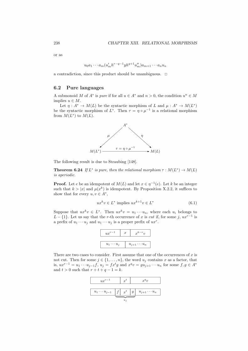
238 CHAPTER XIII. RELATIONAL MORPHISMS
or as
u0a1 · · · am(u′mhr−q−1yhq+1u′′m)am+1 · · · anun
a contradiction, since this product should be unambiguous.
6.2 Pure languages
A submonoid M of A∗ is pure if for all u ∈ A∗ and n > 0, the condition un ∈Mimplies u ∈M .
Let η : A∗ → M(L) be the syntactic morphism of L and µ : A∗ → M(L∗)be the syntactic morphism of L∗. Then τ = η ◦ µ−1 is a relational morphismfrom M(L∗) to M(L).
M(L∗) M(L)
A∗
µ
τ = η ◦ µ−1
η
The following result is due to Straubing [148].
Theorem 6.24 If L∗ is pure, then the relational morphism τ :M(L∗)→M(L)is aperiodic.
Proof. Let e be an idempotent ofM(L) and let x ∈ η−1(e). Let k be an integersuch that k > |x| and µ(xk) is idempotent. By Proposition X.2.2, it suffices toshow that for every u, v ∈ A∗,
uxkv ∈ L∗ implies uxk+1v ∈ L∗ (6.1)
Suppose that uxkv ∈ L∗. Then uxkv = u1 · · ·un, where each ui belongs toL− {1}. Let us say that the r-th occurrence of x is cut if, for some j, uxr−1 isa prefix of u1 · · ·uj and u1 · · ·uj is a proper prefix of uxr.
uxr−1 x xk−rv
u1 · · ·uj uj+1 · · ·un
There are two cases to consider. First assume that one of the occurrences of x isnot cut. Then for some j ∈ {1, . . . , n}, the word uj contains x as a factor, thatis, uxr−1 = u1 · · ·uj−1f , uj = fxtg and xqv = guj+1 · · ·un for some f, g ∈ A∗
and t > 0 such that r + t+ q − 1 = k.
uxr−1 xt xqv
u1 · · ·uj−1 f xt g uj+1 · · ·un
︸ ︷︷ ︸uj

6. THREE EXAMPLES OF RELATIONAL MORPHISMS 239
Since x ∼L x2 and since t > 0, one gets fxtg ∼L fx
t+1g and thus fxt+1g ∈ L.It follows that uxk+1v = u1 · · ·uj−1fx
t+1guj+1 · · ·un ∈ L∗, proving (6.1) in this
case.Suppose now that every occurrence of x is cut. Then for 1 6 r 6 k, there
exists jr ∈ {1, . . . , n} and fr ∈ A∗, gr ∈ A
+ such that
uxr−1fr = u1 · · ·uj , x = frgr and grxk−rv = ujr+1
· · ·un
Since there are |x| factorisations of x of the form fg, and since |x| < k, there existtwo indices r 6= r′ such that fr = fr′ and gr = gr′ . Thus, for some indices i < jand some factorisation x = fg, one has uxr−1f = u1 · · ·ui, gx
sf = ui+1 · · ·ujand gxtv = uj+1 · · ·un. It follows that gxsf = g(fg)sf = (gf)s+1. Sincegxsf ∈ L∗ and since L is pure, gf ∈ L∗. Therefore, uxk+1v = uxr−1xxsxxxtv =(ur−1f)(gxsf)(gf)(gxtv) ∈ L∗, proving (6.1) in this case as well.
Corollary 6.25 If L is star-free and pure, then L∗ is star-free.
Proof. By Theorem X.2.3, L is star-free if and only ifM(L) is aperiodic. Now,if L is pure, the relational morphism τ is aperiodic and henceM(L∗) is aperiodic.It follows that L∗ is star-free.
6.3 Flower automata
Let L be a finite language of A+. The flower automaton of L+ is the finitenondeterministic automaton A = (Q,A,E, I, F ), where Q = {1, 1} ∪ {(u, v) ∈A+ ×A+ | uv ∈ L}, I = F = {(1, 1)}. There are four types of transitions:
{((u, av)
a−→ (ua, v)) | uav ∈ L, (u, v) 6= (1, 1)
}{((u, a)
a−→ (1, 1)) | ua ∈ L, u 6= 1
}{((1, 1)
a−→ (a, v)) | av ∈ L, v 6= 1
}{((1, 1)
a−→ (1, 1)) | a ∈ L
}
It is easy to see that this automaton recognises L+.
Example 6.2 Let A = {a, b} and L = {a, ba, aab, aba}.
(1, 1)
(a, ba)
(ab, a)(a, ab)
(aa, b)
(b, a)
a
a
b
aa
a
b
ba
Figure 6.2. A flower automaton.
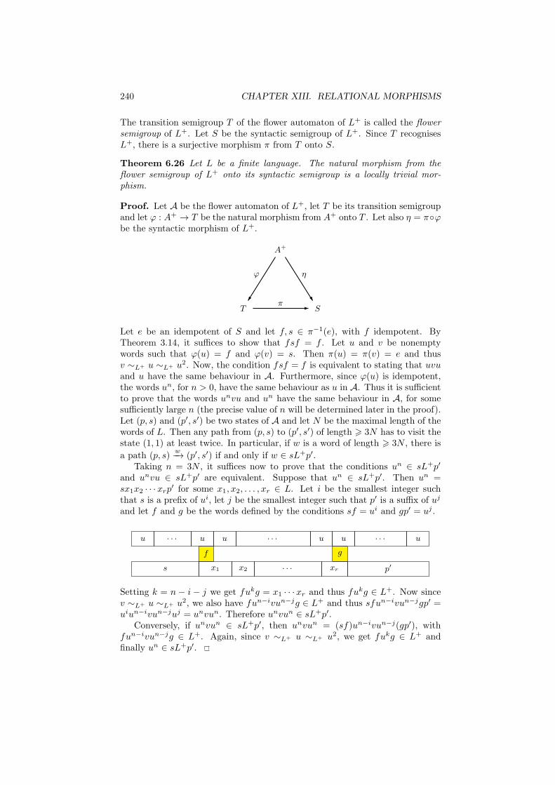
240 CHAPTER XIII. RELATIONAL MORPHISMS
The transition semigroup T of the flower automaton of L+ is called the flowersemigroup of L+. Let S be the syntactic semigroup of L+. Since T recognisesL+, there is a surjective morphism π from T onto S.
Theorem 6.26 Let L be a finite language. The natural morphism from theflower semigroup of L+ onto its syntactic semigroup is a locally trivial mor-phism.
Proof. Let A be the flower automaton of L+, let T be its transition semigroupand let ϕ : A+ → T be the natural morphism from A+ onto T . Let also η = π◦ϕbe the syntactic morphism of L+.
T S
A+
π
ϕ η
Let e be an idempotent of S and let f, s ∈ π−1(e), with f idempotent. ByTheorem 3.14, it suffices to show that fsf = f . Let u and v be nonemptywords such that ϕ(u) = f and ϕ(v) = s. Then π(u) = π(v) = e and thusv ∼L+ u ∼L+ u2. Now, the condition fsf = f is equivalent to stating that uvuand u have the same behaviour in A. Furthermore, since ϕ(u) is idempotent,the words un, for n > 0, have the same behaviour as u in A. Thus it is sufficientto prove that the words unvu and un have the same behaviour in A, for somesufficiently large n (the precise value of n will be determined later in the proof).Let (p, s) and (p′, s′) be two states of A and let N be the maximal length of thewords of L. Then any path from (p, s) to (p′, s′) of length > 3N has to visit thestate (1, 1) at least twice. In particular, if w is a word of length > 3N , there is
a path (p, s)w−→ (p′, s′) if and only if w ∈ sL+p′.
Taking n = 3N , it suffices now to prove that the conditions un ∈ sL+p′
and unvu ∈ sL+p′ are equivalent. Suppose that un ∈ sL+p′. Then un =sx1x2 · · ·xrp
′ for some x1, x2, . . . , xr ∈ L. Let i be the smallest integer suchthat s is a prefix of ui, let j be the smallest integer such that p′ is a suffix of uj
and let f and g be the words defined by the conditions sf = ui and gp′ = uj .
u · · · u u · · · u u · · · u
f g
s x1 x2 · · · xr p′
Setting k = n − i − j we get fukg = x1 · · ·xr and thus fukg ∈ L+. Now sincev ∼L+ u ∼L+ u2, we also have fun−ivun−jg ∈ L+ and thus sfun−ivun−jgp′ =uiun−ivun−juj = unvun. Therefore unvun ∈ sL+p′.
Conversely, if unvun ∈ sL+p′, then unvun = (sf)un−ivun−j(gp′), withfun−ivun−jg ∈ L+. Again, since v ∼L+ u ∼L+ u2, we get fukg ∈ L+ andfinally un ∈ sL+p′.
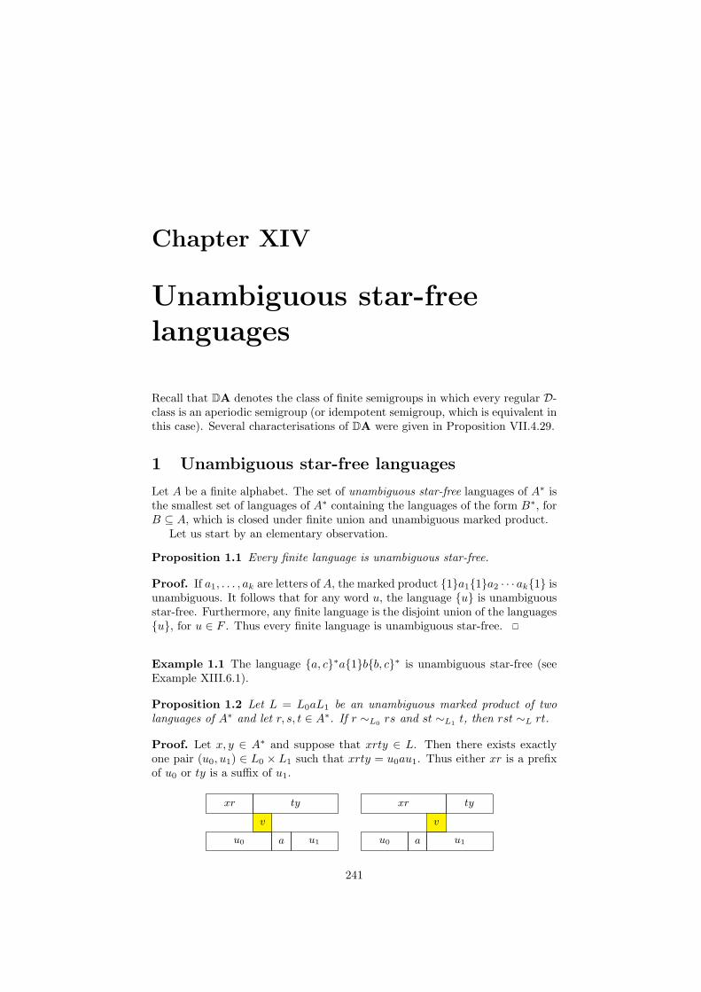
Chapter XIV
Unambiguous star-free
languages
Recall that DA denotes the class of finite semigroups in which every regular D-class is an aperiodic semigroup (or idempotent semigroup, which is equivalent inthis case). Several characterisations of DA were given in Proposition VII.4.29.
1 Unambiguous star-free languages
Let A be a finite alphabet. The set of unambiguous star-free languages of A∗ isthe smallest set of languages of A∗ containing the languages of the form B∗, forB ⊆ A, which is closed under finite union and unambiguous marked product.
Let us start by an elementary observation.
Proposition 1.1 Every finite language is unambiguous star-free.
Proof. If a1, . . . , ak are letters of A, the marked product {1}a1{1}a2 · · · ak{1} isunambiguous. It follows that for any word u, the language {u} is unambiguousstar-free. Furthermore, any finite language is the disjoint union of the languages{u}, for u ∈ F . Thus every finite language is unambiguous star-free.
Example 1.1 The language {a, c}∗a{1}b{b, c}∗ is unambiguous star-free (seeExample XIII.6.1).
Proposition 1.2 Let L = L0aL1 be an unambiguous marked product of twolanguages of A∗ and let r, s, t ∈ A∗. If r ∼L0
rs and st ∼L1t, then rst ∼L rt.
Proof. Let x, y ∈ A∗ and suppose that xrty ∈ L. Then there exists exactlyone pair (u0, u1) ∈ L0 × L1 such that xrty = u0au1. Thus either xr is a prefixof u0 or ty is a suffix of u1.
xr ty
v
u0 a u1
xr ty
v
u0 a u1
241

242 CHAPTER XIV. UNAMBIGUOUS STAR-FREE LANGUAGES
In the first case, one gets xrv = u0 and vau1 = ty for some v ∈ A∗ and sincer ∼L0
rs and xrv ∈ L0, it follows that xrsv ∈ L0 and thus xrsty = xrsvau1 ∈ L.The second case is similar.
Suppose now that xrsty ∈ L. Then there exists exactly one pair (u0, u1) ∈L0 × L1 such that xrsty = u0au1. If xrs is a prefix of u0 or if sty is a suffixof u1, one can use the same argument as above to show that xrty ∈ L. Thecritical case occurs when s = s0as1, xrs0 = u0 and s1ty = u1.
xr s ty
s0 s1
u0 a u1
Then xrs0 ∈ L0 and hence xrss0 ∈ L0 since r ∼L0rs. Similarly, s1sty ∈ L1
since st ∼L1t. It follows that (xrss0)a(s1ty) = xrssty = (xrs0)a(s1sty). This
contradicts the fact that the marked product L0aL1 is unambiguous.
The aim of this section is to prove the following theorem.
Theorem 1.3 A language is unambiguous star-free if and only if its syntacticmonoid is finite and belongs to DA.
Proof. The easiest part of the proof relies on Theorem XIII.6.23. Let
L = L0a1L1 · · · anLn
be an unambiguous marked product. Let M0, . . . , Mn and M be the respectivesyntactic monoids of L0, . . . , Ln and L.
Lemma 1.4 If M0, . . . , Mn belong to DA, so does M .
Proof. Since the monoids M0, . . . , Mn are all in DA, so is their product N .Furthermore, by Theorem XIII.6.23, there is a locally trivial relational mor-
phism τ from M into N . Let Mα−1
−→ Rβ−→ N be the canonical factorisation
of τ . Since M is a quotient of R, it suffices to prove that R belongs to DA. ByTheorem XIII.3.14, β is a locally trivial morphism. Let D be a regular D-classof R. Then β(D) is a regular D-class of N and since N belongs to DA, thisD-class is an aperiodic simple semigroup. In particular, β(D) is in L1 and sinceβ is a locally trivial morphism, the semigroup β−1(β(D)) also belongs to L1.It follows in particular that D is an aperiodic simple semigroup and thus Rbelongs to DA.

Chapter XV
Wreath product
In this chapter, we introduce two important notions: the semidirect productof semigroups and the wreath product of transformation semigroups. We alsoprove some basic decomposition results.
1 Semidirect product
Let S and T be semigroups. We write the product in S additively to provide amore transparent notation, but it is not meant to suggest that S is commutative.A left action of T on S is a map (t, s) 7→ t· s from T 1×S to S such that, for alls, s1, s2 ∈ S and t, t1, t2 ∈ T ,
(1) t1 · (t2 · s) = (t1t2)· s
(2) t· (s1 + s2) = t· s1 + t· s2(3) 1· s = s
If S is a monoid with identity 0, the action is unitary if it satisfies, for all t ∈ T ,
(4) t· 0 = 0
The semidirect product of S and T (with respect to the given action) is thesemigroup S ∗ T defined on S × T by the multiplication
(s, t)(s′, t′) = (s+ t· s′, tt′)
2 Wreath product
Let X = (P, S) and Y = (Q,T ) be two transformation semigroups. To makethe notation more readable, we shall denote the semigroup S and its action onP additively and the semigroup T and its action on Q multiplicatively. Thewreath product of X and Y , denoted by X ◦Y , is the transformation semigroup(P ×Q,W ) where W consists of all pairs (f, t), with f is a function from Q intoS and t ∈ T . Since we are thinking of f as acting on the right on Q, we will usethe more suitable notation q · f in place of f(q). The action of W on P × Q isgiven by
(p, q)· (f, t) = (p+ q · f, q · t) (2.1)
We claim that this action is faithful. Indeed, if (p, q)· (f, t) = (p, q)· (f ′, t′) for all(p, q) ∈ P×Q, then q · t = q · t′ for all q ∈ Q and thus t = t′ since T acts faithfully
243
244 CHAPTER XV. WREATH PRODUCT
on Q. On the other hand, p+ q · f = p+ q · f ′ for all p ∈ P and thus q · f = q · f ′
since S acts faithfully on P . Thus f = f ′, proving the claim. In particular Wcan be considered as a subset of the semigroup of all transformations on P ×Q.We leave it to the reader to verify that W is closed under composition and thatthe product on W is defined by
(f, t)(f ′, t′) = (g, tt′)
where g is defined, for each q ∈ Q by
q · g = q · f + (q · t)· f ′
Let us now verify that Formula (2.1) really defines an action of W on P ×Q. If(p, q) ∈ P ×Q and (f, t), (f ′, t′) ∈W , we have
((p, q)· (f, t)
)· (f ′, t′) = (p+ q · f, q · t)· (f ′, t′) = (p+ q · f + (q · t)· f ′, q · tt′)
= (p, q)((f, t)(f ′, t′)
)
Given two semigroups S and T , consider the wreath product (S1, S)◦ (T 1, T ) =(S1× T 1,W ). The semigroup W is called the wreath product of S and T and isdenoted by S ◦T . The connexions with the semidirect product and the productare given in the next propositions.
Proposition 2.1 Let S and T be semigroups. Then every semidirect product ofS and T is a subsemigroup of S ◦T . Furthermore, S ◦T is a semidirect productof ST 1
and T .
Proof. Let S ∗T be a semidirect product of S and T . Let ϕ : S ∗T → S ◦T bethe function defined by ϕ(s, t) = (f, t) where f : T 1 → S is given by t· f = t· sfor every t ∈ T 1. It is easy to verify that ϕ is a semigroup morphism.
For the second part of the statement, define a left action (t, f) 7→ t· f of T on
ST 1
as follows: t· f is the function from T 1 into S defined by t′ · (t· f) = (t′t)· f .Then the semidirect product defined by this action is isomorphic to S ◦ T .
Proposition 2.2 Let X and Y be transformation semigroups. Then X × Ydivides X ◦ Y .
Proof. Let X = (P, S) and Y = (Q,T ). Since the transformation semigroupsX × Y and X ◦ Y have the same set of states, P × Q, it suffices to show thatS × T can be embedded into SQ × T . With each pair (s, t), associate the pair(f, t), where f is the constant map onto s. Then, for every pair (p, q) ∈ P ×Q,(p, q)· (s, t) = (p + s, q · t) = (p + q · f, q · t) = (p, q)· (f, t), which concludes theproof.
A routine computation shows that the wreath product on transformationsemigroups is associative. The wreath product also preserves division.
Proposition 2.3 If (P1, S1) divides (Q1, T1) and (P2, S2) divides (Q2, T2), then(P1, S1) ◦ (P2, S2) divides (Q1, T1) ◦ (Q2, T2).

3. BASIC DECOMPOSITION RESULTS 245
Proof. Let π1 : Q1 → P1 and π2 : Q2 → P2 be the surjective mappings definingthe divisions. Let π = π1 × π2 : Q1 × Q2 → P1 × P2. For (f, s2) ∈ (P1, S1) ◦
(P2, S2), define (f, s2) = (g, s2) by choosing a cover s2 of s2 and, for eachq2 ∈ Q2, a cover g(q2) of f(π2(q2)). Now, for each (q1, q2) ∈ Q1 ×Q2,
π(q1, q2)· (f, s2) = (π1(q1), π2(q2))· (f, s2) = (π1(q1)· f(π2(q2)), π2(q2)· s2)
= (π1(q1 · g(q2)), π2(q2 · s2)) = π(q1 · g(q2), q2 · s2)
= π((q1, q2)· (g, s2))
and this computation concludes the proof.
In view of Proposition 2.3, we have the following corollary.
Corollary 2.4 If S1 divides T1 and S2 divides T2, then S1 ◦S2 divides T1 ◦T2.
If X = (P, S) is a transformation semigroup, then X1 denotes the transfor-mation semigroup obtained by adjoining to S the identity map 1P on P . If p isa state, we let cp denote the constant map defined, for all q ∈ P , by cp(q) = p.The transformation semigroup obtained by adjoining to S all the constant mapscp is denoted by X.
Proposition 2.5 Let X and Y be transformation semigroups. Then (X ◦ Y )1
divides X1 ◦ Y 1 and X ◦ Y divides X ◦ Y .
Proof. Let X = (P, S) and Y = (Q,T ). First note that the four transformationsemigroups X ◦ Y , X ◦ Y , (X ◦ Y )1 and X1 ◦ Y 1 have the same set of states,P×Q. Next, 1P×Q has the same action as (f, 1Q) ∈ (S1)Q×T , where f(q) = 1Pfor all q ∈ Q. Thus (X ◦ Y )1 embeds into X1 ◦ Y 1.
Finally, if (p, q) ∈ P ×Q, the constant map c(p,q) has exactly the same action
as the pair (g, cq) ∈ SQ× T where g(x) = cp for all x ∈ Q. Thus X ◦ Y embeds
into X ◦ Y .
3 Basic decomposition results
In this section, we give some useful decomposition results. Let us first remindProposition VII.4.21, which gives a useful decomposition result for commutativemonoids. Useful decompositions involving Un and Un are given in the nextpropositions.
Proposition 3.6 For every n > 0, Un divides Un−12 and Un divides Un
2 .
Proof. Arguing by induction on n, it suffices to verify that Un divides Un−1 ×U2. Actually a simple computation shows that Un is isomorphic to the sub-monoid N of Un−1 × U2 defined as follows:
N = {(1, 1)} ∪ {(ai, a1) | 1 6 i 6 n− 1} ∪ {(a1, a2)}
A dual proof works for Un.
A more precise result follows from Proposition IX.1.6: a monoid is idempo-tent and R-trivial if and only if it divides Un
2 for some n > 0. Dually, a monoidis idempotent and L-trivial if and only if it divides Un
2 for some n > 0.
246 CHAPTER XV. WREATH PRODUCT
Proposition 3.7 For every n > 0, Un divides Un ◦ U2.
Proof. Let π : Un×U2 → Un be the surjective partial map defined by π(1, a1) =1 and, for 1 6 i 6 n, π(ai, a2) = ai.
For 1 6 j 6 n, we set aj = (fj , a2) where fj : U2 → Un is defined by1· fj = a2 · fj = 1 and a1 · fj = aj . We also set 1 = (f, 1) where f : U2 → Un isdefined by 1· f = a1 · f = a2 · f = 1. Now a simple verification shows that π isindeed a cover:
π(ai, a2)· 1 = π(ai, a2) = π(ai + a2 · f, a2 · 1) = π((ai, a2)· 1)
π(1, a1)· 1 = π(1, a1) = π(1 + a1 · f, a1 · 1) = π((1, a1)(f, 1)) = π((1, a1)· 1)
π(ai, a2)· aj = ai = π(ai, a2) = π(ai + a2 · fj , a2 · a2) = π((ai, a2)· aj)
π(1, a1)· aj = aj = π(aj , a2) = π(1 + a1 · fj , a1 · a2) = π((1, a1)· aj)
Thus Un divides Un ◦ U2.
The following result now follows immediately from Propositions 3.6 and 3.7.
Corollary 3.8 For every n > 0, Un divides U2 ◦ · · · ◦ U2︸ ︷︷ ︸n+1 times
.
For each n > 0, let Dn be the class of finite semigroups S such that, forall s0, s1, . . . , sn in S, s0s1 · · · sn = s1 · · · sn. In such a semigroup, a productof more than n elements is determined by the last n elements. By PropositionVII.4.15, these semigroups are lefty trivial. We shall now give a decompositionresult for the semigroups in Dn. As a first step, we decompose n as a productof copies of 2.
Lemma 3.9 If 2k > n, then n divides 2k.
Proof. The result is trivial, since if T is any subset of size n of 2k, (T, T ) is asub-transformation semigroup of 2k isomorphic to n.
We now decompose the semigroups of Dn as an iterated wreath product oftransformation semigroups of the form (T, T ).
Proposition 3.10 Let S be a semigroup of Dn and let T = S ∪ {t}, where t isa new element. Then (S1, S) divides (T, T ) ◦ · · · ◦ (T, T )︸ ︷︷ ︸
n times
.
Proof. Let ϕ : Tn → S1 be the partial function defined on sequences of theform (t, . . . , t, xi, . . . , x1), where x1, . . . , xi ∈ S, by
ϕ(t, . . . , t, xi, . . . , x1) =
{xi · · ·x1 if i > 0
1 if i = 0
Clearly ϕ is surjective. If s ∈ S, we set s = (fn−1, . . . , f1, s), where, for 1 6 i 6n− 1, fi : T
i → T is defined by (ti, . . . , t1)· fi = ti. Thus
(tn, . . . , t1)s = (tn−1, . . . , t1, s)

3. BASIC DECOMPOSITION RESULTS 247
It follows that if p = (t, . . . , t, xi, . . . , x1) is in the domain of ϕ, then p· s isalso in the domain of ϕ and ϕ(p· s) = ϕ(p)· s. This proves the proposition.
Proposition 3.10 and Lemma 3.9 now give immediately.
Corollary 3.11 Every semigroup of Dn divides a wreath product of copies of2.
R-trivial monoids admit also a simple decomposition.
Theorem 3.12 A monoid is R-trivial if and only if it divides a wreath productof the form U1 ◦ · · · ◦ U1.
Proof. We first show that every monoid of the form U1 ◦ · · · ◦ U1 is R-trivial.Since U1 itself is R-trivial, and since, by Proposition 2.1, a wreath product isa special case of a semidirect product, it suffices to show that the semidirectproduct S ∗ T of two R-trivial monoids S and T is again R-trivial. Indeed,consider two R equivalent elements (s, t) and (s′, t′) of S∗T . Then, (s, t)(x, y) =(s′, t′) and (s′, t′)(x′, y′) = (s, t) for some elements (x, y) and (x′, y′) of S ∗ T .Therefore, on one hand s + tx = s′ and s′ + t′x′ = s and on the other hand,ty = t′ and t′y′ = t. It follows that s R s′ and t R t′. Therefore s = s′ andt = t′, and S ∗ T is R-trivial.
Let M = {s1, . . . , sn} be an R-trivial monoid of size n. We may assumethat si 6R sj implies j 6 i. Let us identify the elements of Un
1 with words oflength n on the alphabet {0, 1}. Let ϕ : U1 × · · · ×U1 →M be the onto partialfunction defined by
ϕ(1n−j0j) = sj (0 6 j 6 n)
Thus ϕ(u) is not defined if u /∈ 1∗0∗. For each s ∈M , let
s = (fn−1, . . . , f2, a1)
where
a1 =
{1 if s = 1
0 if s 6= 1
and fi+1 : U1 × · · · × U1︸ ︷︷ ︸i times
→ U1 is defined by
fi+1(1i−j0j) =
{1 if sjs = sk and k 6 i
0 if sjs = sk and k > i
If u /∈ 1∗0∗, the value of fi+1(u) can be chosen arbitrarily.Let p = 1n−j0j and s ∈ M . Let k be such that sk = sjs. Since sk 6R sj ,
k > j. Then
ps = (fn−1, . . . , f2, a1)(1n−j0j)
= 1n−k0k
whence ϕ(ps) = sk = sjs = ϕ(p)s. Therefore, M divides U1 ◦ · · · ◦ U1.
As a preparation to the next theorem, we prove another decomposition re-sult, which is important in its own right.

248 CHAPTER XV. WREATH PRODUCT
Proposition 3.13 Let M be a finite aperiodic monoid and let S = M − {1}.Then at least one of the following cases occurs:
(1) M is a monogenic monoid,
(2) M is isomorphic to Un for some n > 0,
(3) there is a proper left ideal I of S and a proper subsemigroup T of S suchthat S = I ∪ T .
Proof. Since M is aperiodic, S is a subsemigroup of M . If S is empty, theresult is trivial. Otherwise, let L1, L2, . . . , Ln be the maximal L-classes of S forthe L-order on L-classes.
If n > 1, then S − Ln is a proper left ideal of S. Indeed, let s ∈ S − Ln
and t ∈ M . Then ts ∈ S − Ln, since otherwise ts ∈ Ln, ts 6L s and s ∈ Ln
by the maximality of Ln. Let T be the subsemigroup generated by Ln. ThenT is a proper subsemigroup since T ∩ L1 = ∅. Moreover S = (S − Ln) ∪ T byconstruction.
We are left with the case n = 1: S has a unique maximal L-class L. Let Tbe the subsemigroup generated by L. Then S = (S − L) ∪ T and S−L is a leftideal of S different from S. If S − L is empty, then L is the minimal ideal ofS and we are in case (2), otherwise S − L is a proper left ideal of S. We nowinspect the case T = S. If L is a singleton, then S is monogenic and we arein case (1). If |L| > 1, then by Proposition V.1.18, L is regular and consists ofL-equivalent idempotents. It follows that T = L = S and we are again in case(2).
Proposition 3.14 Let M be a monoid. Suppose that M = L∪N where L is aleft ideal and N is a submonoid of M . Then M divides L1 ◦N .
Proof. Let ϕ : L1 × N → M be the map defined by ϕ(l, n) = ln. SinceM = L ∪N and L ∪N ⊆ L1N , M = L1N and ϕ is onto.
Recall that N = N ∪ {cn | n ∈ N}, where one extends the product on N bysetting sct = csct = ct and cst = cst for all s, t ∈ N .
Let us construct a covering of M by L1 ◦N . Let m ∈M and let f and g bethe functions from N to L1 defined, for all n ∈ N , by
f(n) = 1 f(cn) = 1
g(n) = nm g(cn) = 1
We now define m ∈ L1 ◦N by setting
m =
{(g, c1) if m ∈ L
(f,m) if m /∈ L
Let (l, n) ∈ L1 ×N . Then
ϕ(l, n)·m = (ln)·m = lnm
Let m ∈M . If m ∈ L, we get
(l, n)· m = (l, n)(g, c1) = (l· g(n), n· c1) = (l· g(n), 1) = (lnm, 1)

3. BASIC DECOMPOSITION RESULTS 249
and since L is a left ideal, lnm ∈ L. On the other hand, if m ∈ N ,
(l, n)· m = (l, n)(f,m) = (l· f(n), n·m) = (l, nm)
and since N is a monoid, nm ∈ N . In both cases, ϕ((l, n)· m) = lnm. It followsthat ϕ is a covering and thus M divides L1 ◦N .
Theorem 3.15 A monoid is aperiodic if and only if it divides a wreath productof the form U2 ◦ · · · ◦ U2.
Proof. Let M be an aperiodic monoid and let S = M − {1}. Consider thethree cases given by Proposition 3.13. If M is monogenic, then it is R-trivial,and the result follows from Theorem 3.12. If M is isomorphic to Un for somen > 0, the result follows from Corollary 3.8. Finally, suppose there is a properleft ideal L of S and a proper subsemigroup T of S such that S = L ∪ T . ThenL is also a left ideal of M and N = T ∪ {1} is a proper submonoid of M . Thusby Proposition 3.14, M divides L1 ◦N .
Arguing by induction on |M |, we may assume that L and N divide wreathproducts of copies of U2. It follows, by Proposition 2.5, that L1 alsos dividewreath products of copies of U2, since U2 = U1
2 and that N divides wreathproducts of copies of U2 = U3. Now, by Proposition 3.6, U3 divides U2 ◦ U2.Finally, M itself divides a wreath product of copies of U2.
Proposition 3.16 Let X = (P, S) be a transformation semigroup such thatP ·S = P . Then 2 ◦X divides X ◦ (R,R), where R is the set {1, 2}P × S.
Proof. Define ϕ : P ×R→ {1, 2}×P by setting ϕ(p, f, s) = (p· f, p· s) for eachp ∈ P , f ∈ {1, 2}P and s ∈ S. Given a transformation v = (g, t) of 2 ◦X, withg ∈ {1, 2}P and t ∈ S, define the transformation v of X ◦ (R,R) by setting
(p, f, s)· v = (p· s, g, t)
then we have
ϕ(p, f, s)· v = (p· f, p· s)(g, t) = (p· f + (p· s)· g, p· st)
((p· s)· g, p· st) = ϕ(p· s, g, t) = ϕ((p, f, s)· v)
Thus 2 ◦X divides X ◦ (R,R).
Given a variety V, we say that a semigroup S is locally in a variety V ifthe local semigroup of each idempotent is in V. For instance, a semigroup S islocally trivial if, for each s ∈ S and e ∈ E(S), ese = e.
We shall present without proof our last decomposition result (see the Notessection).
Proposition 3.17 A semigroup is locally R-trivial if and only if it divides awreath product of the form U1 ◦ · · · ◦ U1 ◦ 2 ◦ · · · ◦ 2.
Proof. TO DO.
We now turn to groups.

250 CHAPTER XV. WREATH PRODUCT
Proposition 3.18 Let π : G → H be a surjective morphism of groups and letK = π−1(1). Then G is isomorphic to a subgroup of K ◦H.
Proof. For each h ∈ H, select an element ph of G such that π(ph) = h. Foreach g ∈ G, define a map g : H → K by setting g(h) = phgp
−1hπ(g). Finally, let
ϕ : G→ K ◦H be the map defined by
ϕ(g) = (g, π(g))
Let us show that ϕ is a group morphism. By Proposition II.3.6, it suffices toprove that ϕ is a semigroup morphism. Let g1, g2 ∈ G and let s1 = π(g1) ands2 = π(g2). One gets
ϕ(g1)ϕ(g2) = (g1, s1)(g2, s2) = (g1 + s1g2, s1s2)
with, for each h ∈ H,
(g1 + s1g2)(h) = g1(h)g2(hs1) = phg1p−1hs1phs1g2p
−1hs1s2
= phg1g2p−1hs1s2
= g1g2(h)
and thus ϕ(g1)ϕ(g2) = ϕ(g1g2).Finally, we prove that ϕ is injective. If ϕ(g1) = ϕ(g2), then π(g1) = π(g2) = s
and g1(1) = g2(1), that is, p1g1p−1s = p1g2p
−1s , whence g1 = g2. It follows that
G is isomorphic to a subgroup of K ◦H.
A subgroup H of a group G is normal if, for each h in H and each g in G,the element hgh−1 is still in H. A group G is soluble if there is an ascendingchain of subgroups 1 = G0 ⊆ G1 ⊆ · · · ⊆ Gn = G such that, for 1 6 i 6 n,Gi−1 is normal in Gi and Gi/Gi−1 is a commutative group.
Proposition 3.19 A group is soluble if and only if it divides a wreath productof cyclic groups.
Proof. TO DO.
Theorem 3.20 (Krohn-Rhodes) Let M be a monoid. Then there exists asequence G1, . . . , Gn of groups dividing M and a sequence M0, . . . ,Mn of ape-riodic monoids such that M divides M0 ◦G1 ◦M1 · · · ◦Gn ◦Mn.
Proof. TO DO.
4 Exercises
Section 3
1. Show that any finite inverse monoid divides a semidirect product of theform S ∗G, where S an idempotent and commutative monoid and G is a finitegroup. Actually, a stronger result holds: a finite monoid divides the semidirectproduct of an idempotent and commutative monoid by a group if and only ifits idempotents commute.

Chapter XVI
Sequential functions
So far, we have only used automata to define languages but more powerfulmodels allow one to define functions or even relations between words. Theseautomata not only read an input word but they also produce an output. Suchdevices are also called transducers. In the deterministic case, which forms thetopic of this chapter, they define the so called sequential functions. The com-position of two sequential functions is also sequential.
Straubing’s “wreath product principle” [146, 151] provides a description ofthe languages recognised by the wreath product of two monoids. It has nu-merous applications, including Schutzenberger’s theorem on star-free languages[31, 81], the characterisation of languages recognised by solvable groups [146] orthe expressive power of fragments of temporal logic [30, 164].
1 Definitions
1.1 Pure sequential transducers
A pure sequential transducer is an 6-tuple T = (Q,A,R, q0, · , ∗), where Q isa finite set of states, A is a finite alphabet called the input alphabet, R is asemigroup (possibly infinite) called the output semigroup, q0 ∈ Q is the initialstate, (q, a) 7→ q · a ∈ Q and (q, a) 7→ q ∗ a ∈ R are partial functions with thesame domain contained in Q×A, called respectively the transition function andthe output function. Both functions are conveniently represented in Figure 1.1,in which the vertical slash is a separator.
q q · aa | q ∗ a
Figure 1.1. A transition and its output function.
The transition and the output functions can be extended to partial functions
251
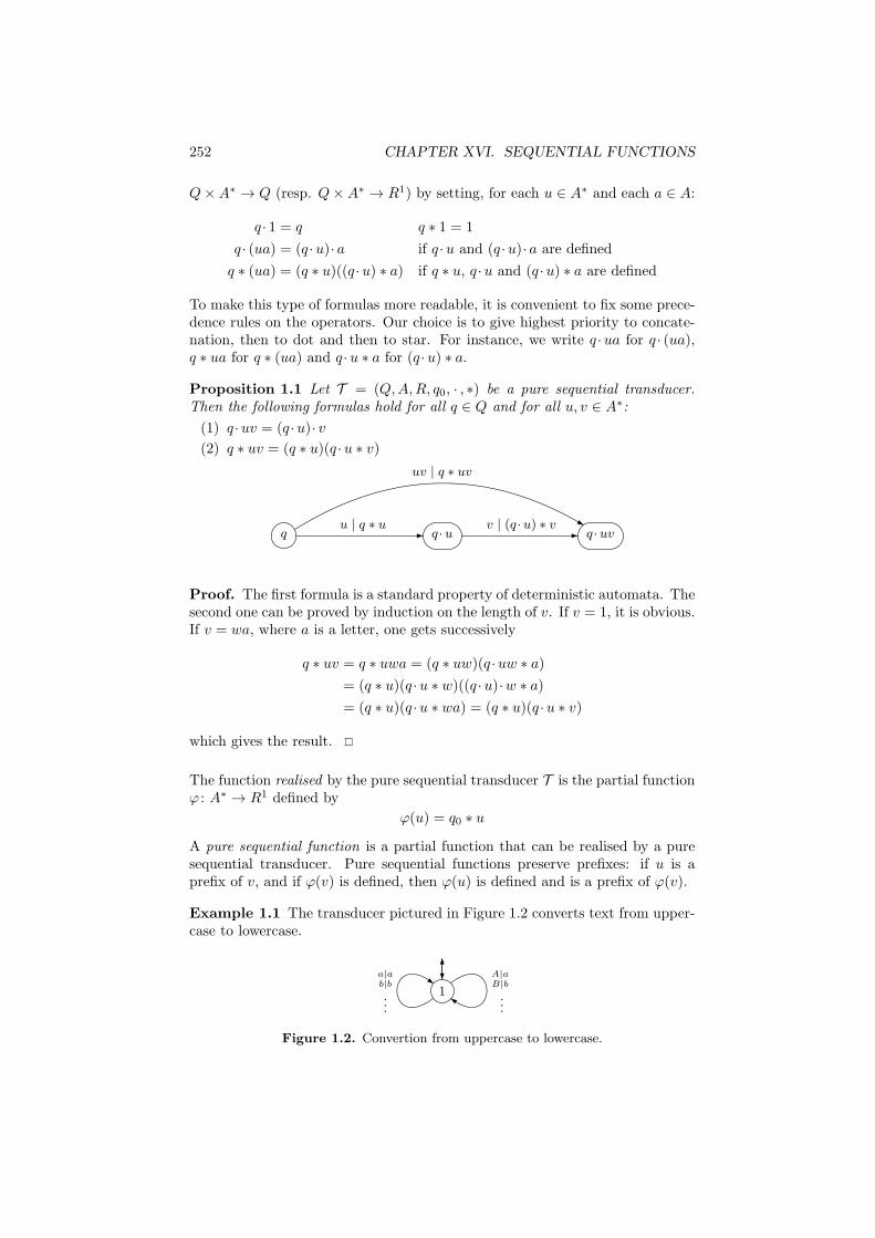
252 CHAPTER XVI. SEQUENTIAL FUNCTIONS
Q×A∗ → Q (resp. Q×A∗ → R1) by setting, for each u ∈ A∗ and each a ∈ A:
q · 1 = q q ∗ 1 = 1
q · (ua) = (q ·u)· a if q ·u and (q ·u)· a are defined
q ∗ (ua) = (q ∗ u)((q ·u) ∗ a) if q ∗ u, q ·u and (q ·u) ∗ a are defined
To make this type of formulas more readable, it is convenient to fix some prece-dence rules on the operators. Our choice is to give highest priority to concate-nation, then to dot and then to star. For instance, we write q ·ua for q · (ua),q ∗ ua for q ∗ (ua) and q ·u ∗ a for (q ·u) ∗ a.
Proposition 1.1 Let T = (Q,A,R, q0, · , ∗) be a pure sequential transducer.Then the following formulas hold for all q ∈ Q and for all u, v ∈ A∗:
(1) q ·uv = (q ·u)· v
(2) q ∗ uv = (q ∗ u)(q ·u ∗ v)
q q ·u q ·uvu | q ∗ u v | (q ·u) ∗ v
uv | q ∗ uv
Proof. The first formula is a standard property of deterministic automata. Thesecond one can be proved by induction on the length of v. If v = 1, it is obvious.If v = wa, where a is a letter, one gets successively
q ∗ uv = q ∗ uwa = (q ∗ uw)(q ·uw ∗ a)
= (q ∗ u)(q ·u ∗ w)((q ·u)·w ∗ a)
= (q ∗ u)(q ·u ∗ wa) = (q ∗ u)(q ·u ∗ v)
which gives the result.
The function realised by the pure sequential transducer T is the partial functionϕ : A∗ → R1 defined by
ϕ(u) = q0 ∗ u
A pure sequential function is a partial function that can be realised by a puresequential transducer. Pure sequential functions preserve prefixes: if u is aprefix of v, and if ϕ(v) is defined, then ϕ(u) is defined and is a prefix of ϕ(v).
Example 1.1 The transducer pictured in Figure 1.2 converts text from upper-case to lowercase.
1
a|ab|b
...
A|aB|b
...
Figure 1.2. Convertion from uppercase to lowercase.
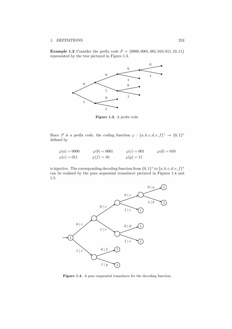
1. DEFINITIONS 253
Example 1.2 Consider the prefix code P = {0000, 0001, 001, 010, 011, 10, 11}represented by the tree pictured in Figure 1.3.
b
b0
b0
b0b0
b1
b1
b1
b0
b1
b1b0
b1
Figure 1.3. A prefix code.
Since P is a prefix code, the coding function ϕ : {a, b, c, d, e, f}∗ → {0, 1}∗
defined by
ϕ(a) = 0000 ϕ(b) = 0001 ϕ(c) = 001 ϕ(d) = 010
ϕ(e) = 011 ϕ(f) = 10 ϕ(g) = 11
is injective. The corresponding decoding function from {0, 1}∗ to {a, b, c, d, e, f}∗
can be realised by the pure sequential transducer pictured in Figures 1.4 and1.5.
1
1
1
1
1
1
1
1
1 | ε
0 | ε
1 | g
0 | f
1 | ε
0 | ε
1 | e
0 | d
1 | c
0 | ε
1 | b
0 | a
Figure 1.4. A pure sequential transducer for the decoding function.
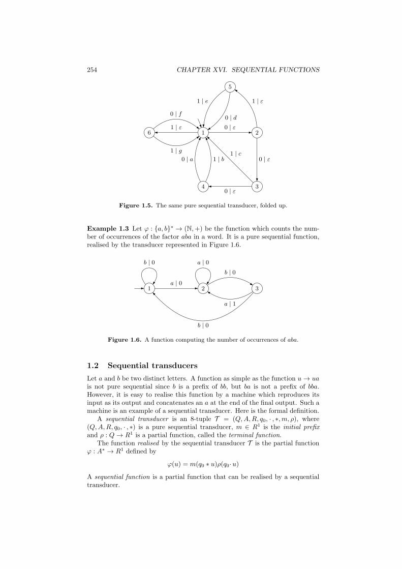
254 CHAPTER XVI. SEQUENTIAL FUNCTIONS
1 2
34
5
60 | ε
0 | ε1 | c
0 | ε
1 | ε
0 | a
0 | d0 | f
1 | ε
1 | b
1 | e
1 | g
Figure 1.5. The same pure sequential transducer, folded up.
Example 1.3 Let ϕ : {a, b}∗ → (N,+) be the function which counts the num-ber of occurrences of the factor aba in a word. It is a pure sequential function,realised by the transducer represented in Figure 1.6.
1 2 3a | 0
b | 0 a | 0
b | 0
a | 1
b | 0
Figure 1.6. A function computing the number of occurrences of aba.
1.2 Sequential transducers
Let a and b be two distinct letters. A function as simple as the function u→ uais not pure sequential since b is a prefix of bb, but ba is not a prefix of bba.However, it is easy to realise this function by a machine which reproduces itsinput as its output and concatenates an a at the end of the final output. Such amachine is an example of a sequential transducer. Here is the formal definition.
A sequential transducer is an 8-tuple T = (Q,A,R, q0, · , ∗,m, ρ), where(Q,A,R, q0, · , ∗) is a pure sequential transducer, m ∈ R1 is the initial prefixand ρ : Q→ R1 is a partial function, called the terminal function.
The function realised by the sequential transducer T is the partial functionϕ : A∗ → R1 defined by
ϕ(u) = m(q0 ∗ u)ρ(q0·u)
A sequential function is a partial function that can be realised by a sequentialtransducer.

2. COMPOSITION OF SEQUENTIAL FUNCTIONS 255
Example 1.4 Let u, v ∈ A∗. The map ϕ : A∗ → A∗ defined by ϕ(x) = uxv isrealised by the sequential transducer represented in Figure 1.7. Its initial prefixis u and its terminal function ρ is defined by ρ(1) = v.
u v1
a | a
Figure 1.7. A sequential transducer realising the function x → uxv.
Example 1.5 The function ϕ : A∗ → A∗ defined by ϕ(x) = x(ab)−1 is realisedby the sequential transducer represented in Figure 1.8.
1 11 2 3
a | 1 b | 1
a | ab
b | abb
b | b a | a
Figure 1.8. A sequential transducer realising the function x → x(ab)−1.
Example 1.6 In the reverse binary representation, a binary word a0a1 · · · anrepresents the number
∑06i6n ai2
i. For instance, the word 1011 represents1 + 4 + 8 = 13. Multiplication by 3 can then be performed by the followingsequential transducer.
0 1 20 | 0 1 | 1
1 | 1 1 | 0
0 | 00 | 1ε 1 01
Figure 1.9. A sequential transducer realising the multiplication by 3.
For instance, on the input 1011, which represents 13, the output would be111001, which represents 1 + 2 + 4 + 32 = 39.
2 Composition of sequential functions
The goal of this section is to establish that the composition of two [pure] se-quential functions is also a [pure] sequential function.

256 CHAPTER XVI. SEQUENTIAL FUNCTIONS
Let ϕ : A∗ → B∗ and θ : B∗ → C∗ be two pure sequential functions, realisedrespectively by the pure sequential transducers
A = (Q,A,B, q0, · , ∗) and B = (P,B,C, p0, · , ∗)
The composition of these two functions can be realised by feeding B with theoutput of A. This observation leads to the following definition. The wreathproduct of B by A is the pure sequential transducer
B ◦ A = (P ×Q,A,C, (p0, q0), · , ∗)
defined by
(p, q)· a = (p· (q ∗ a), q · a) and (p, q) ∗ a = p ∗ (q ∗ a)
(p, q) (p· (q ∗ a), q · a)a | p ∗ (q ∗ a)
Figure 2.10. A transition and its output in B ◦ A.
Intuitively, the second component of (p, q) is used to simulate A. The first com-ponent and the output function are obtained by using the output of a transitionin A as input in B.
q q · aa | q ∗ a
p p· (q ∗ a)(q ∗ a) | p ∗ (q ∗ a)
Figure 2.11. The ouput of A as input of B.
This definition can be extended to sequential transducers as follows. Let
A = (Q,A,B, q0, · , ∗, n, ρ) and B = (P,B,C, p0, · , ∗,m, σ)
be two sequential transducers. The wreath product of B by A is the sequentialtransducer
B ◦ A = (P ×Q,A,C, (p0 ·n, q0), · , ∗,m(p0 ∗ n), ω)
defined by
(p, q)· a = (p· (q ∗ a), q · a)
(p, q) ∗ a = p ∗ (q ∗ a)
ω(p, q) = (p ∗ ρ(q))σ(p· ρ(q))
The computation of the initial prefix and of the terminal function are illustratedin Figure 2.12.

2. COMPOSITION OF SEQUENTIAL FUNCTIONS 257
q0n
p0m n | p0 ∗ n
Figure 2.12. The initial prefix.
The next proposition describes the behaviour of B ◦ A.
Proposition 2.2 The following formulas hold for all states (p, q) of B ◦A andfor all u ∈ A∗:
(p, q)·u = (p· (q ∗ u), q ·u)
(p, q) ∗ u = p ∗ (q ∗ u)
Proof. We prove the result by induction on the length of u. If u = 1, one getson the one hand (p, q)· 1 = (p, q) and on the other hand q ∗ 1 = 1 and q · 1 = q,whence (p· (q ∗ 1), q · 1) = (p· 1, q) = (p, q), which proves the first formula. Thesecond one is trivial since by definition (p, q) ∗ 1 = 1 = p ∗ (q ∗ 1).
Suppose by induction that the formulas are true for a word u of length nand let a be a letter. Setting v = ua, w = q ∗ u and w′ = (q ·u) ∗ a, one getsq ∗ v = q ∗ (ua) = (q ∗ u)((q ·u) ∗ a) = ww′ and
(p, q)· v = (p· (q ∗ u), q ·u)· a = (p·w, q ·u)· a
= (p·w· (q ·u ∗ a), (q ·u)· a) = (p·ww′, q · v) = (p· (q ∗ v), q · v)
which proves the first formula. Furthermore
(p, q) ∗ v =((p, q) ∗ u)
)((p, q)·u ∗ a
)=
(p ∗ (q ∗ u)
)((p· (q ∗ u), q ·u
)∗ a
)
= (p ∗ w)((p·w, q ·u) ∗ a
)= (p ∗ w)
((p·w) ∗ (q ·u ∗ a)
)
= (p ∗ w)((p·w) ∗ w′
)= p ∗ (ww′) = p ∗ (q ∗ v)
which gives the second one.
Example 2.1 Let A = {a, b}, B = {a, b} and C = {a, b, c} and let A and B bethe pure sequential transducers represented in Figure 2.13.
1 2
1 2
3
a | aa b | a
b | ab b | 1b | b
a | b
a | a
a | ba | c
b | cc
Figure 2.13. The transducers A (on the left) and B (on the right).

258 CHAPTER XVI. SEQUENTIAL FUNCTIONS
The wreath product B ◦ A is defined by the formula
(1, 1)· a = (3, 1) (1, 1) ∗ a = ab (1, 1)· b = (1, 2) (1, 1) ∗ b = ab
(1, 2)· a = (1, 1) (1, 2) ∗ a = ab (1, 2)· b = (2, 2) (1, 2) ∗ b = a
(2, 1)· a = (1, 1) (2, 1) ∗ a = bc (2, 1)· b = (2, 2) (2, 1) ∗ b = 1
(2, 2)· a = (2, 1) (2, 2) ∗ a = 1 (2, 2)· b = (3, 2) (2, 2) ∗ b = b
(3, 1)· a = (2, 1) (3, 1) ∗ a = ca (3, 1)· b = (2, 2) (3, 1) ∗ b = cc
(3, 2)· a = (2, 1) (3, 2) ∗ a = cc (3, 2)· b = (1, 2) (3, 2) ∗ b = c
and is represented in Figure 2.14.
1, 1
1, 2
2, 1
2, 2
3, 1 3, 2
a | ab
b | a
a | bc
b | b
a | ca
b | cc
a | cc
b | 1a | 1b | aba | ab
b | c
Figure 2.14. The wreath product B ◦ A.
Theorem 2.3 Let A and B be two [pure] sequential transducers realising thefunctions ϕ : A∗ → B∗ and θ : B∗ → C∗. Then B◦A realises the function θ ◦ϕ.
Proof. Let A = (Q,A,B, q0, · , ∗, n, ρ) and B = (P,B,C, p0, · , ∗,m, σ) be twosequential transducers realising the fonctions ϕ : A∗ → B∗ and θ : B∗ → C∗,respectively. Let η be the function realised by B ◦ A and let u ∈ A∗. Settingp = p0 ·n, q = q0 ·u and v = q0 ∗ u, one gets ϕ(u) = n(q0 ∗ u)ρ(q0 ·u) = nvρ(q).The computation of η(u) gives
η(u) = m(p0 ∗ n)((p, q0) ∗ u)ω((p, q0)·u)
= m(p0 ∗ n)(p ∗ (q0 ∗ u))ω(p· (q0 ∗ u), q0 ·u)
= m(p0 ∗ n)(p ∗ v)ω(p· v, q)
Furthermore, one has
ω(p· v, q) = (p· v ∗ ρ(q))σ((p· v)· ρ(q))
= (p· v ∗ ρ(q))σ(p· vρ(q))
= (p· v ∗ ρ(q))σ(p0 ·nvρ(q))
= (p· v ∗ ρ(q))σ(p0 ·ϕ(u))
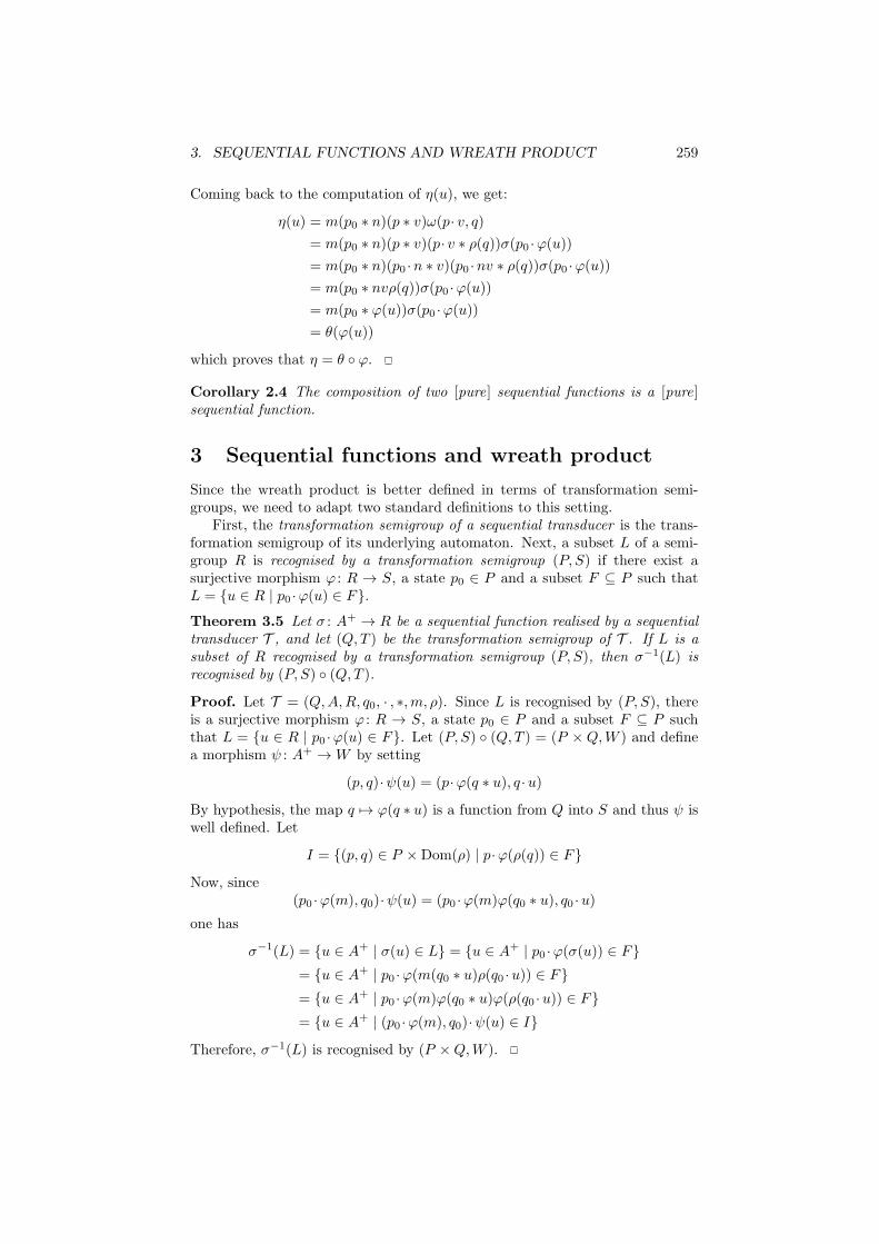
3. SEQUENTIAL FUNCTIONS AND WREATH PRODUCT 259
Coming back to the computation of η(u), we get:
η(u) = m(p0 ∗ n)(p ∗ v)ω(p· v, q)
= m(p0 ∗ n)(p ∗ v)(p· v ∗ ρ(q))σ(p0 ·ϕ(u))
= m(p0 ∗ n)(p0 ·n ∗ v)(p0 ·nv ∗ ρ(q))σ(p0 ·ϕ(u))
= m(p0 ∗ nvρ(q))σ(p0 ·ϕ(u))
= m(p0 ∗ ϕ(u))σ(p0 ·ϕ(u))
= θ(ϕ(u))
which proves that η = θ ◦ ϕ.
Corollary 2.4 The composition of two [pure] sequential functions is a [pure]sequential function.
3 Sequential functions and wreath product
Since the wreath product is better defined in terms of transformation semi-groups, we need to adapt two standard definitions to this setting.
First, the transformation semigroup of a sequential transducer is the trans-formation semigroup of its underlying automaton. Next, a subset L of a semi-group R is recognised by a transformation semigroup (P, S) if there exist asurjective morphism ϕ : R → S, a state p0 ∈ P and a subset F ⊆ P such thatL = {u ∈ R | p0 ·ϕ(u) ∈ F}.
Theorem 3.5 Let σ : A+ → R be a sequential function realised by a sequentialtransducer T , and let (Q,T ) be the transformation semigroup of T . If L is asubset of R recognised by a transformation semigroup (P, S), then σ−1(L) isrecognised by (P, S) ◦ (Q,T ).
Proof. Let T = (Q,A,R, q0, · , ∗,m, ρ). Since L is recognised by (P, S), thereis a surjective morphism ϕ : R → S, a state p0 ∈ P and a subset F ⊆ P suchthat L = {u ∈ R | p0 ·ϕ(u) ∈ F}. Let (P, S) ◦ (Q,T ) = (P ×Q,W ) and definea morphism ψ : A+ →W by setting
(p, q)·ψ(u) = (p·ϕ(q ∗ u), q ·u)
By hypothesis, the map q 7→ ϕ(q ∗ u) is a function from Q into S and thus ψ iswell defined. Let
I = {(p, q) ∈ P ×Dom(ρ) | p·ϕ(ρ(q)) ∈ F}
Now, since(p0 ·ϕ(m), q0)·ψ(u) = (p0 ·ϕ(m)ϕ(q0 ∗ u), q0 ·u)
one has
σ−1(L) = {u ∈ A+ | σ(u) ∈ L} = {u ∈ A+ | p0 ·ϕ(σ(u)) ∈ F}
= {u ∈ A+ | p0 ·ϕ(m(q0 ∗ u)ρ(q0 ·u)) ∈ F}
= {u ∈ A+ | p0 ·ϕ(m)ϕ(q0 ∗ u)ϕ(ρ(q0 ·u)) ∈ F}
= {u ∈ A+ | (p0 ·ϕ(m), q0)·ψ(u) ∈ I}
Therefore, σ−1(L) is recognised by (P ×Q,W ).
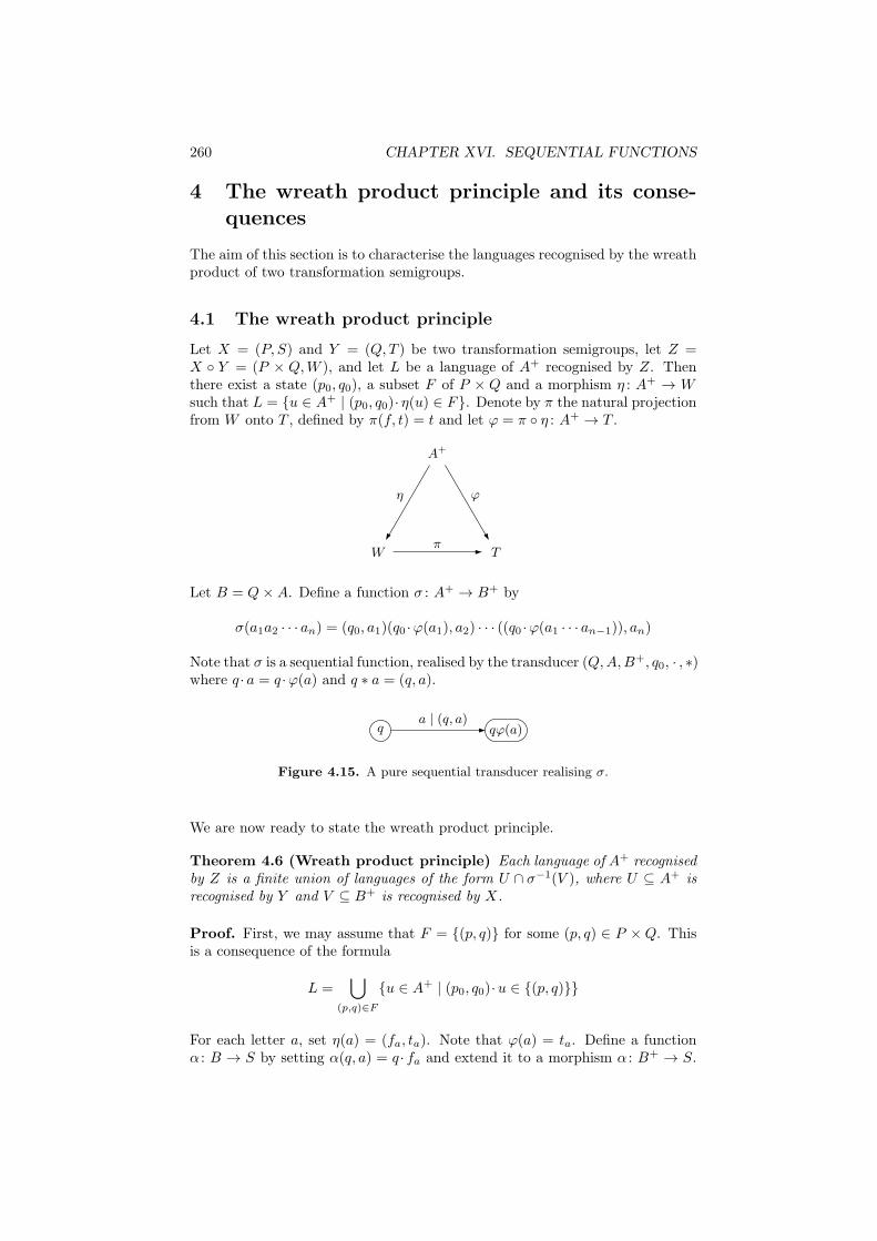
260 CHAPTER XVI. SEQUENTIAL FUNCTIONS
4 The wreath product principle and its conse-
quences
The aim of this section is to characterise the languages recognised by the wreathproduct of two transformation semigroups.
4.1 The wreath product principle
Let X = (P, S) and Y = (Q,T ) be two transformation semigroups, let Z =X ◦ Y = (P × Q,W ), and let L be a language of A+ recognised by Z. Thenthere exist a state (p0, q0), a subset F of P × Q and a morphism η : A+ → Wsuch that L = {u ∈ A+ | (p0, q0)· η(u) ∈ F}. Denote by π the natural projectionfrom W onto T , defined by π(f, t) = t and let ϕ = π ◦ η : A+ → T .
A+
TW
η ϕ
π
Let B = Q×A. Define a function σ : A+ → B+ by
σ(a1a2 · · · an) = (q0, a1)(q0 ·ϕ(a1), a2) · · · ((q0 ·ϕ(a1 · · · an−1)), an)
Note that σ is a sequential function, realised by the transducer (Q,A,B+, q0, · , ∗)where q · a = q ·ϕ(a) and q ∗ a = (q, a).
q qϕ(a)a | (q, a)
Figure 4.15. A pure sequential transducer realising σ.
We are now ready to state the wreath product principle.
Theorem 4.6 (Wreath product principle) Each language of A+ recognisedby Z is a finite union of languages of the form U ∩ σ−1(V ), where U ⊆ A+ isrecognised by Y and V ⊆ B+ is recognised by X.
Proof. First, we may assume that F = {(p, q)} for some (p, q) ∈ P ×Q. Thisis a consequence of the formula
L =⋃
(p,q)∈F
{u ∈ A+ | (p0, q0)·u ∈ {(p, q)}}
For each letter a, set η(a) = (fa, ta). Note that ϕ(a) = ta. Define a functionα : B → S by setting α(q, a) = q · fa and extend it to a morphism α : B+ → S.
5. APPLICATIONS OF THE WREATH PRODUCT PRINCIPLE 261
Let u = a1a2 · · · an be a word. Then
(p0, q0)·u = (p0, q0)· (fa1, ta1
)(fa2, ta2
) · · · (fan, tan
)
=(p0 + q0 · fa1
+ · · ·+ (q0 · ta1· · · tan−1
)fan, q0 · ta1
· · · tan
)
=(p0 + α(q0, a1) + · · ·+ α(q0 ·ϕ(a1 · · · an−1), an), q0 ·ϕ(u)
)
=(p0 + α(σ(u)), q0 ·ϕ(u)
)
It follows that (p0, q0)·u = (p, q) if and only if the following two conditions aresatisfied:
(1) p0 + α(σ(u)) = p,
(2) q0 ·ϕ(u) = q.
Setting U = {u ∈ A+ | q0 ·ϕ(u) = q} and V = {v ∈ B+ | p0 + α(v) = p},condition (1) can be reformulated as u ∈ σ−1(V ), and condition (2) as u ∈ U .Thus
L = U ∩ σ−1(V )
Now, U is recognised by Y and V is recognised by X, which concludes theproof.
We now derive a variety version of Theorem 4.6. It is stated for the case whereboth V and W are varieties of monoids, but similar statements hold if V or Wis a variety of semigroups. Let us define the variety V ∗W as the class of alldivisors of wreath products of the form S ◦ T with S ∈ V and T ∈W.
Corollary 4.7 Let V and W be two varieties of monoids and let U be thevariety of languages associated with V ∗W. Then, for every alphabet A, U(A∗)is the smallest lattice containing W(A∗) and the languages of the form σ−1
ϕ (V ),where σϕ is the sequential function associated with a morphism ϕ : A∗ → T ,with T ∈W and V ∈ V((A× T )∗).
Proof. Since W is contained in V ∗W, W(A∗) is contained in U(A∗). Fur-thermore, if V and σϕ are given as in the statement, then σ−1
ϕ (V ) ∈ U(A∗) byTheorem 3.5.
It follows from the definition of V ∗W and from Proposition IV.4.25 thatevery language of U(A∗) is recognised by a wreath product of the form S ◦ T ,with S ∈ V and T ∈W. Theorem 4.6 now suffices to conclude.
5 Applications of the wreath product principle
In this section, we give several applications of the wreath product principle. Westudy the operations L 7→ LaA∗ and L 7→ La, where a is a letter of A. Then wegive a description of the languages corresponding to J1 ∗V, Jyx = xK ∗V andr1 ∗V, where V is a variety of monoids (resp. semigroups).
5.1 The operations T 7→ U1 ◦ T and L 7→ LaA∗
The study of this operation is based on the following proposition.

262 CHAPTER XVI. SEQUENTIAL FUNCTIONS
Proposition 5.8 Let A be an alphabet, let a ∈ A and let L be a language ofA∗ recognised by a monoid T . Then LaA∗ is recognised by the wreath productU1 ◦ T .
Proof. Let ϕ : A∗ → T be a morphism recognising L, let B = T × A and letσϕ : A
∗ → B∗ be the sequential function associated with ϕ. Let P = ϕ(L) andC = {(p, a) | p ∈ P}. Then we have
σ−1ϕ (B∗CB∗) = {a1a2 · · · an ∈ A
∗ | σϕ(a1a2 · · · an) ∈ B∗CB∗}
= {a1a2 · · · an ∈ A∗ | there exists an i such that
(ϕ(a1a2 · · · ai−1), ai) ∈ C}
= {a1a2 · · · an ∈ A∗ | there exists an i such that
ai = a and a1a2 · · · ai−1 ∈ ϕ−1(P )}
= LaA∗
Since B∗CB∗ is recognised by U1, the proposition follows from Theorem 3.5.
Proposition 5.8 leads to the following result on varieties.
Theorem 5.9 Let V be a variety of monoids and let V be the correspondingvariety. Then the variety W which corresponds to J1 ∗V is defined as follows.For each alphabet A, W(A∗) is the Boolean algebra generated by the languagesL and LaA∗, where a ∈ A and L ∈ V(A∗).
Proof. For each alphabet A, let V ′(A∗) denote the Boolean algebra generatedby the languages L and LaA∗, where a ∈ A and L ∈ V(A∗).
We first show that V ′(A∗) ⊆ W(A∗). Since J1 ∗ V contains V, W(A∗)contains V(A∗). Let L ∈ V(A∗) and a ∈ A. Then L is recognised by somemonoid T of V and, by Proposition 5.8, LaA∗ is recognised by U1 ◦ T . Thismonoid belongs to J1 ∗V and hence LaA∗ ∈ W(A∗).
To establish the opposite inclusion, it suffices now, by Corollary 4.7, toverify that L ∈ V ′(A∗) for every language L of the form σ−1
ϕ (V ), where σϕ isthe sequential function associated with a morphism of monoids ϕ : A∗ → T ,with T ∈ V and V is a subset of (T × A)∗ recognised by a monoid of J1. LetB = T × A. By Proposition IX.1.4, V is a Boolean combination of languagesof the form B∗CB∗, for some subset C of T × A. Since Boolean operationscommute with σ−1
ϕ , we may assume that V = B∗CB∗, where C = (t, a) forsome (t, a) ∈ B. In this case
L = {u ∈ A∗ | σϕ(u) ∈ B∗CB∗}
= {a1a2 · · · an ∈ A∗ | (ϕ(a1 · · · ai−1), ai) = (t, a) for some i} (5.1)
= ϕ−1(t)aA∗
Now, ϕ−1(t) is recognised by T and thus ϕ−1(t) ∈ V(A∗). It follows thatϕ−1(t)aA∗ ∈ V ′(A∗) and thus L ∈ V ′(A∗). Therefore W(A∗) ⊆ V ′(A∗).

5. APPLICATIONS OF THE WREATH PRODUCT PRINCIPLE 263
5.2 The operations T 7→ 2 ◦ T and L 7→ La
Recall that 2 denotes the transformation semigroup ({1, 2}, {1, 2}) with theaction defined by r· s = s. The results are quite similar to those presented inSection 5.1, but the monoid U1 is now replaced by 2.
Proposition 5.10 Let A be an alphabet, let a ∈ A and let L be a language ofA∗ recognised by a monoid T . Then La is recognised by the wreath product 2◦T .
Proof. Let ϕ : A∗ → T be a morphism recognising L, let B = T × A and letσϕ : A
∗ → B∗ be the sequential function associated with ϕ. Let P = ϕ(L) andC = {(p, a) | p ∈ P}. Then we have
σ−1ϕ (B∗C) = {u ∈ A∗ | σϕ(u) ∈ B
∗C}
= {a1a2 · · · an ∈ A+ | (ϕ(a1a2 · · · an−1), an) ∈ C}
= {a1a2 · · · an ∈ A+ | an = a and a1a2 · · · an−1 ∈ ϕ
−1(P )}
= La
Since the language B∗C is recognised by 2, the proposition now follows fromTheorem 3.5.
A result similar to Proposition 5.10 holds if T is a semigroup which is not amonoid. The proof is left as an exercise to the reader.
Proposition 5.11 Let A be an alphabet, let a ∈ A and let L be a language ofA+ recognised by an semigroup T such that T 6= T 1. Then the languages Laand {a} are recognised by the wreath product 2 ◦ (T 1, T ).
We now turn to varieties. Observe that the semigroup 2 generates the varietyJyx = xK.
Theorem 5.12 Let V be a variety of monoids and let V be the correspondingvariety. Let W be the variety corresponding to Jyx = xK ∗ V. Then, for eachalphabet A, W(A+) is the lattice generated by the languages L (contained inA+) or La, where a ∈ A and L ∈ V(A∗).
Proof. For each alphabet A, let V ′(A+) be the lattice generated by the lan-guages L (contained in A+) or La, where a ∈ A and L ∈ V(A∗).
We first show that V ′(A+) ⊆ W(A+). Since Jyx = xK ∗V contains V, everylanguage of V(A∗) contained in A+ is also inW(A+). Let L ∈ V(A∗) and a ∈ A.Then L is recognised by some monoid T of V and, by Proposition 5.10, La isrecognised by 2 ◦ T . Now this semigroup belongs to Jyx = xK ∗ V and thusLa ∈ W(A+).
To establish the opposite inclusion, it suffices now, by Corollary 4.7, toverify that L ∈ V ′(A+) for every language L of the form σ−1
ϕ (V ), where σϕis the sequential function associated with a morphism of monoids ϕ : A∗ → T ,with T ∈ V, and V is a language of (T × A)+ recognised by a transformationsemigroup of Jyx = xK. Let B = T ×A. Then V is a finite union of languages ofthe form B∗c, for some letter c ∈ B. Since union commutes with σ−1
ϕ , we mayassume that V = B∗c, where c = (t, a) for some (t, a) ∈ B. In this case
L = {u ∈ A+ | σϕ(u) ∈ B∗c}
= {a1a2 · · · an ∈ A+ | (ϕ(a1 · · · an−1), an) = (t, a)}
= ϕ−1(t)a
264 CHAPTER XVI. SEQUENTIAL FUNCTIONS
Now, ϕ−1(t) is recognised by T and thus ϕ−1(t) ∈ V(A∗). It follows thatϕ−1(t)a ∈ V ′(A+) for each letter a and thus L ∈ V ′(A+). Therefore W(A+) ⊆V ′(A+).
The semigroup version of Theorem 5.12 can be obtained by using Proposition5.11 instead of Proposition 5.10. Recall that B(1, 2) denotes the semigroup{a, b} equipped the multiplication defined by aa = ba = a and ab = bb = b.
Theorem 5.13 Let V be a variety of semigroups which is not a variety ofgroups, and let V be the corresponding variety. Let W be the variety corre-sponding to Jyx = xK ∗V. Then, for each alphabet A, W(A+) is the Booleanalgebra generated by the languages L, {a} or La, where a ∈ A and L ∈ V(A+).
Recall that the variety r1 is defined by the identity yxω = xω. It is knownto be the smallest variety of semigroups containing B(1, 2) and closed undersemidirect product [40]. Therefore, Theorems 5.12 and 5.13 lead to a languageinterpretation of the operation V→ r1 ∗V.
Corollary 5.14 Let V be a variety of monoids and let V be the correspondingpositive variety. Let W be the positive variety corresponding to r1 ∗V. Then,for each alphabet A, W(A+) is the smallest lattice containing V(A∗) and closedunder the operation L 7→ Lu, for each u ∈ A∗.
Corollary 5.15 Let V be a variety of ordered semigroups which is not a varietyof groups and let V be the corresponding positive variety. Let W be the positivevariety corresponding to r1 ∗ V. Then, for each alphabet A, W(A+) is thesmallest lattice containing V(A+) and the languages {a}, for each a ∈ A, andclosed under the operation L 7→ Lu, for each u ∈ A∗.
5.3 The operation T 7→ U2 ◦ T and star-free expressions
Recall that U2 denotes the monoid {1, a1, a2} defined by a1a1 = a2a1 = a1 anda1a2 = a2a2 = a2.
Proposition 5.16 Let A be an alphabet and let T be a monoid. Then everylanguage of A∗ recognised by U2 ◦ T is a Boolean combination of languages ofthe form K or Ka(LbA∗)c where a, b ∈ A and K and L are recognised by T .
Proof. Let L be a language of A∗ recognised by U2 ◦ T and let B = T × A.The wreath product principle tells us that L is a finite union of languages of theform U ∩ σ−1(V ), where U ⊆ A∗ is recognised by T and V ⊆ B∗ is recognisedby U2. By Proposition IX.1.7, every language of B∗ recognised by U2 is aBoolean combination of languages of the form B∗bC∗, where b ∈ B and C ⊆ B.Therefore, it suffices to prove that a language of the form σ−1(V ) has the rightform. We claim that
σ−1(B∗bC∗) = ϕ−1(m)a
( ⋃
(n,c)/∈C
ϕ−1((mϕ(a)
)−1n)cA∗
)c
(5.2)
Indeed, let b = (t, a) and let u = a1a2 · · · an be a word of A∗. Then σ(u) be-longs to B∗bC∗ if and only if there exists an i such that ϕ(a1a2 · · · ai−1) =
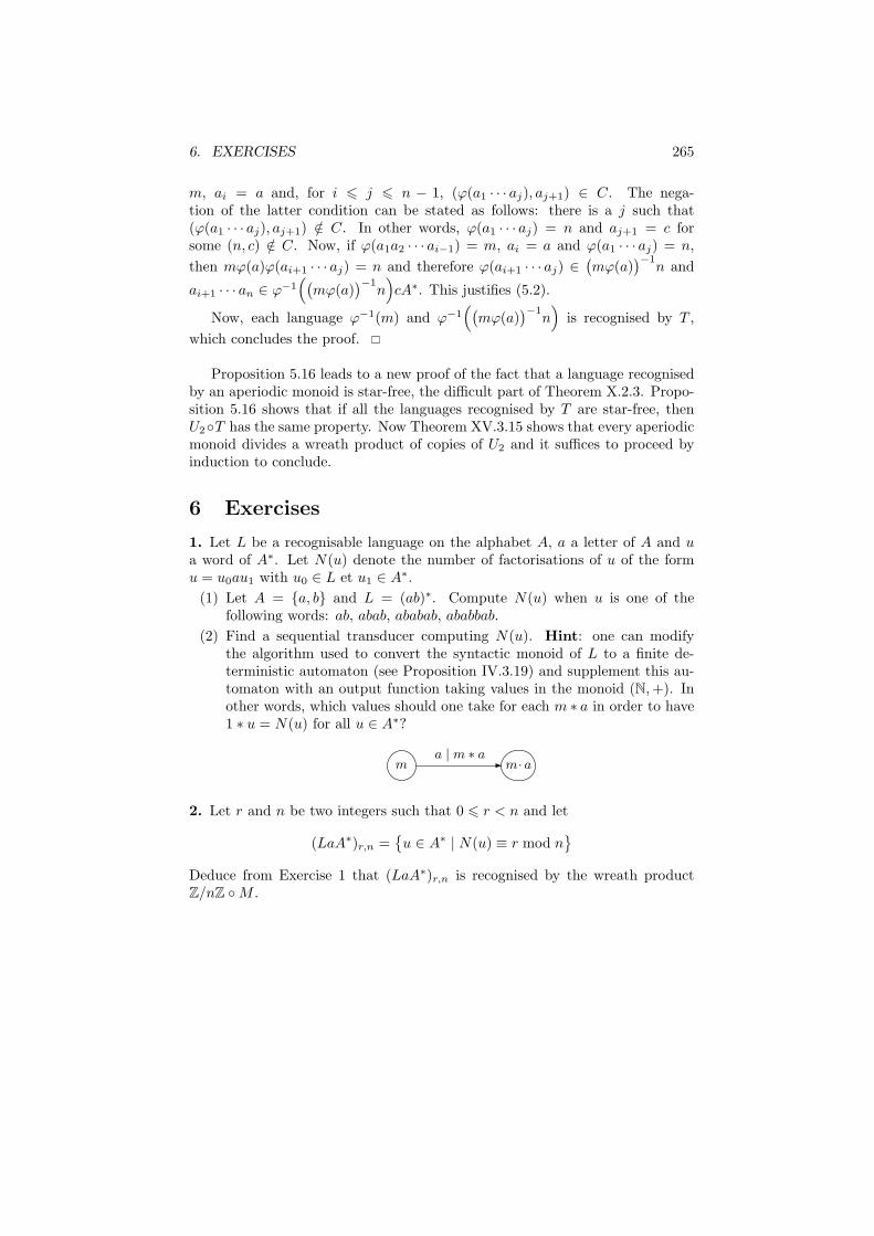
6. EXERCISES 265
m, ai = a and, for i 6 j 6 n − 1, (ϕ(a1 · · · aj), aj+1) ∈ C. The nega-tion of the latter condition can be stated as follows: there is a j such that(ϕ(a1 · · · aj), aj+1) /∈ C. In other words, ϕ(a1 · · · aj) = n and aj+1 = c forsome (n, c) /∈ C. Now, if ϕ(a1a2 · · · ai−1) = m, ai = a and ϕ(a1 · · · aj) = n,
then mϕ(a)ϕ(ai+1 · · · aj) = n and therefore ϕ(ai+1 · · · aj) ∈(mϕ(a)
)−1n and
ai+1 · · · an ∈ ϕ−1
((mϕ(a)
)−1n)cA∗. This justifies (5.2).
Now, each language ϕ−1(m) and ϕ−1((mϕ(a)
)−1n)
is recognised by T ,
which concludes the proof.
Proposition 5.16 leads to a new proof of the fact that a language recognisedby an aperiodic monoid is star-free, the difficult part of Theorem X.2.3. Propo-sition 5.16 shows that if all the languages recognised by T are star-free, thenU2◦T has the same property. Now Theorem XV.3.15 shows that every aperiodicmonoid divides a wreath product of copies of U2 and it suffices to proceed byinduction to conclude.
6 Exercises
1. Let L be a recognisable language on the alphabet A, a a letter of A and ua word of A∗. Let N(u) denote the number of factorisations of u of the formu = u0au1 with u0 ∈ L et u1 ∈ A
∗.
(1) Let A = {a, b} and L = (ab)∗. Compute N(u) when u is one of thefollowing words: ab, abab, ababab, ababbab.
(2) Find a sequential transducer computing N(u). Hint: one can modifythe algorithm used to convert the syntactic monoid of L to a finite de-terministic automaton (see Proposition IV.3.19) and supplement this au-tomaton with an output function taking values in the monoid (N,+). Inother words, which values should one take for each m ∗ a in order to have1 ∗ u = N(u) for all u ∈ A∗?
m m· aa | m ∗ a
2. Let r and n be two integers such that 0 6 r < n and let
(LaA∗)r,n ={u ∈ A∗ | N(u) ≡ r mod n
}
Deduce from Exercise 1 that (LaA∗)r,n is recognised by the wreath productZ/nZ ◦M .

266 CHAPTER XVI. SEQUENTIAL FUNCTIONS

Chapter XVII
Concatenation hierarchies
In the seventies, several classification schemes for the rational languages wereproposed, based on the alternate use of certain operators (union, complemen-tation, product and star). Some forty years later, although much progress hasbeen done, several of the original problems are still open. Furthermore, theirsignificance has grown considerably over the years, on account of the successivediscoveries of links with other fields, like non commutative algebra [40], finitemodel theory [158], structural complexity [15] and topology [77, 94, 97].
Roughly speaking, the concatenation hierarchy of a given class of recognis-able languages is built by alternating Boolean operations (union, intersection,complement) and polynomial operations (union and marked product). For in-stance, the Straubing-Therien hierarchy [157, 147, 149] is based on the emptyand full languages of A∗ and the group hierarchy is built on the group-languages,the languages recognised by a finite permutation automaton. It can be shownthat, if the basis of a concatenation hierarchy is a variety of languages, then ev-ery level is a positive variety of languages [7, 8, 111], and therefore correspondsto a variety of finite ordered monoids [94]. These varieties are denoted by Vn
for the Straubing-Therien hierarchy and Gn for the group hierarchy.
1 Concatenation hierarchies
In this section, we introduce a hierarchy among star-free languages of A∗, knownas the Straubing-Therien’s hierarchy, or concatenation hierarchy.1 For historicalreasons, this hierarchy is indexed by half-integers. The level 0 consists of thelanguages ∅ and A∗. The other levels are defined inductively as follows:
(1) the level n+ 1/2 is the class of union of marked products of languages oflevel n;
(2) the level n+1 is the class of Boolean combination of languages of markedproducts of level n.
We call the levels n (for some nonegative integer n) the full levels and the levelsn+ 1/2 the half levels.
1A similar hierarchy, called the dot-depth hierarchy was previously introduced by Brzo-
zowski, but the Straubing-Therien’s hierarchy is easier to define.
267
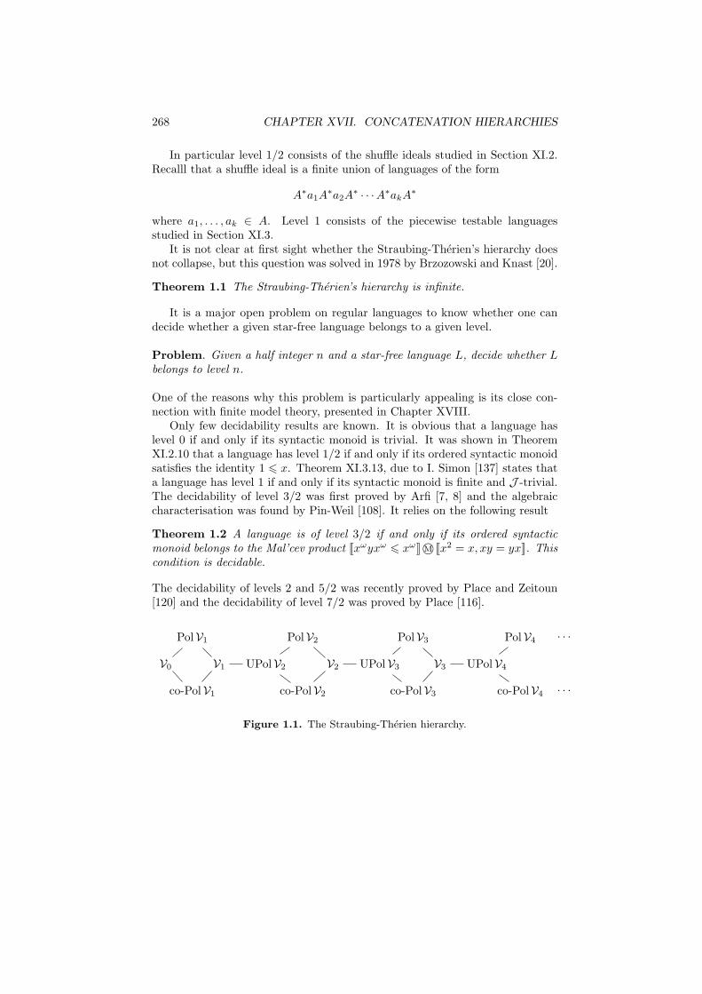
268 CHAPTER XVII. CONCATENATION HIERARCHIES
In particular level 1/2 consists of the shuffle ideals studied in Section XI.2.Recalll that a shuffle ideal is a finite union of languages of the form
A∗a1A∗a2A
∗ · · ·A∗akA∗
where a1, . . . , ak ∈ A. Level 1 consists of the piecewise testable languagesstudied in Section XI.3.
It is not clear at first sight whether the Straubing-Therien’s hierarchy doesnot collapse, but this question was solved in 1978 by Brzozowski and Knast [20].
Theorem 1.1 The Straubing-Therien’s hierarchy is infinite.
It is a major open problem on regular languages to know whether one candecide whether a given star-free language belongs to a given level.
Problem. Given a half integer n and a star-free language L, decide whether Lbelongs to level n.
One of the reasons why this problem is particularly appealing is its close con-nection with finite model theory, presented in Chapter XVIII.
Only few decidability results are known. It is obvious that a language haslevel 0 if and only if its syntactic monoid is trivial. It was shown in TheoremXI.2.10 that a language has level 1/2 if and only if its ordered syntactic monoidsatisfies the identity 1 6 x. Theorem XI.3.13, due to I. Simon [137] states thata language has level 1 if and only if its syntactic monoid is finite and J -trivial.The decidability of level 3/2 was first proved by Arfi [7, 8] and the algebraiccharacterisation was found by Pin-Weil [108]. It relies on the following result
Theorem 1.2 A language is of level 3/2 if and only if its ordered syntacticmonoid belongs to the Mal’cev product Jxωyxω 6 xωK M©Jx2 = x, xy = yxK. Thiscondition is decidable.
The decidability of levels 2 and 5/2 was recently proved by Place and Zeitoun[120] and the decidability of level 7/2 was proved by Place [116].
PolV1 PolV2 PolV3 PolV4 . . .
V0 V1 UPolV2 V2 UPolV3 V3 UPolV4
co-PolV1 co-PolV2 co-PolV3 co-PolV4 . . .
Figure 1.1. The Straubing-Therien hierarchy.

Chapter XVIII
An excursion into logic
1 Introduction
The links between finite automata, languages and logic were first discovered byBuchi [22] and Elgot [41]. Their main result states that monadic second orderhas the same expressive power as finite automata.
The formalism of logic is introduced in Section 2. This section can be skippedby a reader with some background in logic. We detail the interpretation offormulas on words. This amounts mainly to considering a word as a structureby associating with each positive integer i the letter in position i. The relationsthat are used are the order relation between the indices and the relation a(i)expressing that the letter in position i is an a.
In Section 3, we prove the equivalence between finite automata and monadicsecond-order logic (Buchi’s theorem). The conversion from automata to logic isobtained by writing a formula expressing that a word is the label of a successfulpath in an automaton. The opposite direction is more involved and requires tointerpret formulas with free variables as languages over extended alphabets.
In Section 4, we present the corresponding theory for first-order logic. Weprove McNaughton’s theorem [80], stating that first-order logic of the linearorder captures star-free languages.
In Section 4.2, we describe the hierarchy of the first-order logic of the linearorder, corresponding to the alternate use of existential and universal quanti-fiers. We show that this hierarchy corresponds, on words, to the concatenationhierarchy described in Chapter VII. This leads to a doubly satisfying situation:first-order formulas not only correspond globally to a natural class of recognis-able sets (the star-free sets), but this correspondence holds level by level.
2 The formalism of logic
In this section, we review some basic definitions of logic: first-order logic, second-order, monadic second-order and weak monadic second-order logic.
2.1 Syntax
Let us start by defining the syntax of first-order logic.
269
270 CHAPTER XVIII. AN EXCURSION INTO LOGIC
The basic ingredients are the logical symbols which encompass the logicalconnectives: ∧ (and), ∨ (or), ¬ (not), → (implies), the equality symbol =, thequantifiers ∃ (there exists) and ∀ (for all), an infinite set of variables (most oftendenoted by x, y, z, or x0, x1, x2,. . . ) and parenthesis (to ensure legibility of theformulas).
In addition to these logical symbols, we make use of a set L of nonlogicalsymbols, called the signature of the first-order language. These auxiliary sym-bols can be of three types: relation symbols (for instance <), function symbols(for instance min), or constant symbols (for instance 0, 1). Expressions are builtfrom the symbols of L by obeying the usual rules of the syntax, then first-orderformulas are built by using the logical symbols, and are denoted by FO[L]. Wenow give a detailed description of the syntactic rules to obtain the logical for-mulas in three steps, passing successively, following the standard terminology,from terms to atomic formulas and subsequently to formulas.
We first define the set of L-terms. It is the least set of expressions containingthe variables, the constant symbols of L (if there are any) which is closed underthe following formation rule: if t1, t2, . . . , tn are terms and if f is a functionsymbol with n arguments, then the expression f(t1, t2, . . . , tn) is a term. Inparticular, if L does not contain any function symbol, the only terms are thevariables and the constant symbols.
Example 2.1 Let us take as set of nonlogical symbols
L = { < , g, 0}
where < is a binary relation symbol, g is a two-variable function symbol and 0is a constant. Then the following expressions are terms:
x0 g(0, 0) g(x1, g(0, x2)) g(g(x0, x1), g(x1, x2))
The atomic formulas are formulas either of the form
(t1 = t2)
where t1 and t2 are terms, or of the form
R(t1, . . . , tn)
where t1, . . . , tn are terms and R is a n-ary relation symbol of L.
Example 2.2 Continuing Example 2.1, the following expressions are atomicformulas:
(g(x1, g(0, x2)) = x1) (g(0, 0) < 0)
(g(g(x0, x1), g(x1, x2)) < g(x3, x1))
Notice that, in order to improve legibility, we did not apply literally the defi-nition of atomic formulas: indeed, since < is a symbol of binary relation, oneshould write <(t1, t2) instead of t1 < t2.
Finally, the first-order formulas on L form the least set of expressions con-taining the atomic formulas and closed under the following formation rules:
2. THE FORMALISM OF LOGIC 271
(i) If (ϕi)i∈I is a finite family of first-order formulas, so are the expressions
(∧
i∈I
ϕi) and (∨
i∈I
ϕi)
(ii) If ϕ and ψ are first-order formulas, so are the expressions
¬ϕ and (ϕ→ ψ)
(iii) If ϕ is a first-order formula and if x is a variable, then the expressions
(∃xϕ) and (∀xϕ)
are first-order formulas.
To make notations easier, we set
true =∧
i∈∅
ϕi and false =∨
i∈∅
ϕi
Example 2.3 The following expressions are first-order formulas of our examplelanguage:
(∃x (∀y ((y < g(z, 0)) ∧ (x < 0)))) (∀x (y = x))
Again, it is convenient to simplify notation by suppressing some of the paren-thesis and we shall write the previous formulas under the form
∃x ∀y (y < g(x, 0)) ∧ (z < 0) ∀x y = x
In a first-order formula, some variables occur after a quantifier (existential oruniversal): the occurrences of these variables are said to be bounded and theother occurrences are said to be free. For example, in the formula
∃x (y < h(x, 0)) ∧ ∀y (z < y)
the simply underlined occurrences of x and y are bounded and the occurrencesof z and y doubly underlined are free. A variable is free if at least one of itsoccurrences is free. The set FV (ϕ) of free variables of a formula ϕ can bedefined inductively as follows:
(1) If ϕ is an atomic formula, FV (ϕ) is the set of variables occurring in ϕ,
(2) FV (¬ϕ) = FV (ϕ)
(3) FV (∧
i∈I ϕi) = FV (∨
i∈I ϕi) =⋃
i∈I FV (ϕi)
(4) FV (ϕ→ ψ) = FV (ϕ) ∪ FV (ψ)
(5) FV (∃xϕ) = FV (∀xϕ) = FV (ϕ)− {x}
A sentence is a formula in which all occurrences of variables are bounded. Forexample, the formula
∃x ∀y (y < f(x, 0))
is a sentence.We let ϕ(x1, x2, . . . , xn) denote a formula ϕ in which the set of free variables
is contained in {x1, . . . , xn} (but is not necessarily equal to {x1, . . . , xn}).

272 CHAPTER XVIII. AN EXCURSION INTO LOGIC
The variables used in first-order logic, or first-order variables, are interpreted,as we shall see, as the elements of a set. In second-order logic, one makesuse of another type of variables, called second-order variables, which representrelations. These variables are traditionally denoted by capital letters: X0, X1,etc.. One builds in this way the set of second-order formulas on L, denotedby SO[L]. The set of terms is the same as for first-order logic. The atomicformulas are either of the form
(t1 = t2)
where t1 and t2 are terms, or of the form
R(t1, . . . , tn) or X(t1, . . . , tn)
where t1, . . . , tn are terms, R is an n-ary relation symbol of L and X is a variablerepresenting a n-ary relation.
Finally, second-order formulas on L form the least set of expressions con-taining the atomic formulas and closed under the following formation rules:
(i) If ϕ and ψ are second-order formulas, then so are
¬ϕ, (ϕ ∧ ψ), (ϕ ∨ ψ), (ϕ→ ψ)
(ii) If ϕ is a second-order formula, if x is a first-order variable and if X is arelation variable, then the expressions
(∃xϕ) (∀xϕ) (∃Xϕ) (∀Xϕ)
are second-order formulas.
Monadic second-order logic is the fragment of second-order logic in which theonly relation variables are unary relation variables, in other words, variablesrepresenting subsets of the domain. By convenience, they are called set vari-ables. We let MSO(L) denote the set of monadic second-order formulas on L.We shall also use the notation x ∈ X instead of X(x).
2.2 Semantics
We have adopted so far a syntactic point of view to define formulas with noreference to semantics. But of course, formulas would be uninteresting if theywere meaningless. Giving a precise meaning to formulas requires to specify thedomain on which we want to interpret each of the symbols of the language L.Formally, a structure S on L is given by a nonempty set D, called domain andby a map defined on L, called an assignment which associates
(1) with each n-ary relation symbol of L, a n-ary relation defined on D,
(2) with each n-ary function symbol f of L, a n-ary function defined on D,
(3) with each constant symbol c of L, an element of D.
To improve notation, we shall use the same notation for the relation [function,constant] symbols and for the relations [functions, constants] represented bythese symbols. The context will allow us to determine easily what the notationstands for. For example, we shall always employ the symbol < to designate theusual order relation on a set of integers, independently of the domain (N, Z, ora subset of N).
2. THE FORMALISM OF LOGIC 273
We still have to interpret variables. Let us start by first-order variables.Given a fixed structure S on L, with domain D, a valuation on S is a map νfrom the set of variables into the set D. It is then easy to extend ν to a functionof the set of terms of L into D, by induction on the formation rules of terms:
(1) If c is a constant symbol, we put ν(c) = c,
(2) if f is a n-ary function symbol and if t1, . . . , tn are terms,
ν(f(t1, . . . , tn)
)= f(ν(t1) . . . ν(tn))
If ν is a valuation and a an element of D, we let ν(ax
)denote the valuation ν′
defined by
ν′(y) =
{ν(y) if y 6= x
a if y = x
The notion of interpretation can now be easily formalised. Define, for eachfirst-order formula ϕ and for each valuation ν, the expressions “the valuation νsatisfies ϕ in S”, or “S satisfies ϕ[ν]”, denoted by S |= ϕ[ν], as follows:
(1) S |= (t1 = t2)[ν] if and only if ν(t1) = ν(t2)
(2) S |= R(t1, . . . , tn)[ν] if and only if(ν(t1), . . . , ν(tn)
)∈ R
(3) S |= ¬ϕ[ν] if and only if not S |= ϕ[ν]
(4) S |= (∧
i∈I
ϕ)[ν] if and only if for each i ∈ I, S |= ϕi[ν]
(5) S |= (∨
i∈I
ϕ)[ν] if and only if there exists i ∈ I, S |= ϕi[ν]
(6) S |= (ϕ→ ψ)[ν] if and only if S 6|= ϕ[ν] or S |= ψ[ν]
(7) S |= (∃xϕ)[ν] if and only if S |= ϕ[ν(ax
)] for some a ∈ D
(8) S |= (∀xϕ)[ν] if and only if S |= ϕ[ν(ax
)] for each a ∈ D
Note that, actually, the truth of the expression “the valuation ν satisfies ϕ inS” only depends on the values taken by the free variables of ϕ. In particular,if ϕ is a sentence, the choice of the valuation is irrelevant. Therefore, if ϕ is asentence, one says that ϕ is satisfied by S (or that S satisfies ϕ), and denote byS |= ϕ, if, for each valuation ν, S |= ϕ[ν].
Next we move to the interpretation of second-order formulas. Given a struc-ture S on L, with domain D, a second-order valuation on S is a map ν whichassociates with each first-order variable an element of D and with each n-aryrelation variable a subset of Dn (i.e. a n-ary relation on D).
If ν is a valuation and R a subset of Dn, ν(RX
)denotes the valuation ν′
defined by
ν′(x) = ν(x) if x is a first-order variable
ν′(Y ) =
{ν(Y ) if Y 6= X
R if Y = X
The notion of an interpretation, already defined for first-order logic, is supple-

274 CHAPTER XVIII. AN EXCURSION INTO LOGIC
mented by the following rules:
(9) S |= (X(t1, . . . , tn))[ν] if and only if(ν(t1), . . . , ν(tn)
)∈ ν(X)
(10) S |= (∃Xϕ)[ν] if and only if there exists R ⊆ Dn, S |= ϕ[ν(RX
)]
(11) S |= (∀Xϕ)[ν] if and only if for each R ⊆ Dn, S |= ϕ[ν(RX
)]
Weak monadic second-order logic has the same formulas as monadic second-order logic, but the interpretation is even more restricted: only valuations whichassociate with set variables finite subsets of the domain D are considered.
Two formulas ϕ and ψ are said to be logically equivalent if, for each structureS on L, we have S |= ϕ if and only if S |= ψ.
It is easy to see that the following formulas are logically equivalent:
(1) ϕ ∧ ψ and ¬(¬ϕ ∨ ¬ψ)
(2) ϕ→ ψ and ¬ϕ ∨ ψ
(3) ∀xϕ and ¬(∃x ¬ϕ)
(4) ϕ ∨ ψ and ψ ∨ ϕ
(5) ϕ ∧ ψ and ψ ∧ ϕ
(6) ϕ ∧ false and false
(7) ϕ ∨ false and ϕ
Consequently, up to logical equivalence, we may assume that the formulas arebuilt without the symbols ∧, → and ∀.
Logical equivalence also permits one to give a more structured form to for-mulas. A formula is said to be in disjunctive normal form if it can be writtenas a disjunction of conjunctions of atomic formulas or of negations of atomicformulas, in other words in the form
∨
i∈I
∧
j∈Ji
(ϕij ∨ ¬ψij)
where I and the Ji are finite sets, and ϕij and ψij are atomic formulas. Thenext result is standard and easily proved.
Proposition 2.1 Every quantifier free formula is logically equivalent to a quan-tifier free formula in disjunctive normal form.
One can set up a hierarchy inside first-order formulas as follows. Let Σ0 = Π0
be the set of quantifier-free formulas. Next, for each n > 0, denote by Σn+1 theleast set ∆ of formulas such that
(1) ∆ contains all Boolean combinations of formulas of Σn,
(2) ∆ is closed under finite disjunctions and conjunctions,
(3) if ϕ ∈ ∆ and if x is a variable, ∃xϕ ∈ ∆.
Similarly, let Πn+1 denote the least set Γ of formulas such that
(1) Γ contains all Boolean combinations of formulas of Πn,
(2) Γ is closed under finite disjunctions and conjunctions,
(3) if ϕ ∈ Γ and if x is a variable, ∀xϕ ∈ Γ.

2. THE FORMALISM OF LOGIC 275
In particular, Σ1 is the set of existential formulas, that is, formulas of the form
∃x1 ∃x2 . . . ∃xk ϕ
where ϕ is quantifier-free.Finally, we let BΣn denote the set of Boolean combinations of formulas of
Σn.A first-order formula is said to be in prenex normal form if it is of the form
ψ = Q1x1 Q2x2 . . . Qnxn ϕ
where the Qi are existential or universal quantifiers (∃ or ∀) and ϕ is quantifier-free. The sequence Q1x1 Q2x2 . . . Qnxn, which can be considered as a wordon the alphabet
{ ∃x1, ∃x2, . . . , ∀x1, ∀x2, . . . },
is called the quantifier prefix of ψ. The interest in formulas in prenex normalform comes from the following result.
Proposition 2.2 Every first-order formula is logically equivalent to a formulain prenex normal form.
Proof. It suffices to verify that if the variable x does not occur in the formulaψ then
∃x(ϕ ∧ ψ) ≡ (∃xϕ) ∧ ψ
∃x(ϕ ∨ ψ) ≡ (∃xϕ) ∨ ψ
and the same formulas hold for the quantifier ∀. Hence it is possible, by renamingthe variables, to move the quantifiers to the outside.
Proposition 2.2 can be improved to take into account the level of the formulain the Σn hierarchy.
Proposition 2.3 For each integer n > 0,
(1) Every formula of Σn is logically equivalent to a formula in prenex normalform in which the quantifier prefix is a sequence of n (possibly empty)alternating blocks of existential and universal quantifiers, starting with ablock of existential quantifiers.
(2) Every formula of Πn is logically equivalent to a formula in prenex normalform in which the quantifier prefix is a sequence of n (possibly empty)alternating blocks of existential and universal quantifiers, starting with ablock of universal quantifiers.
For example, the formula
∃x1 ∃x2 ∃x3︸ ︷︷ ︸block 1
∀x4 ∀x5︸ ︷︷ ︸block 2
∃x6 ∃x7︸ ︷︷ ︸block 3
ϕ(x1, . . . , x6)
belongs to Σ3 (and also to all Σn with n > 3). Similarly the formula
︸︷︷︸block 1
∀x4 ∀x5︸ ︷︷ ︸block 2
∃x6 ∃x7︸ ︷︷ ︸block 3
ϕ(x1, . . . , x7)

276 CHAPTER XVIII. AN EXCURSION INTO LOGIC
belongs to Σ3 and to Π2, but not to Σ2, since the counting of blocks of a Σn-formula should always begin by a possibly empty block of existential quantifiers.
One can also introduce normal forms and a hierarchy for monadic second-order formulas. Thus, one can show that every monadic second-order formulais logically equivalent to a formula of the form
ψ = Q1X1 Q2X2 . . . QnXn ϕ
where theQi are existential or universal quantifiers and ϕ is a first-order formula.
2.3 Logic on words
The logical language that we shall use now was introduced by Buchi under thename of “sequential calculus”. To interpret formulas on words, one considerseach word as a map associating a letter with each index. Let u = a0a1 . . . an−1,where a0, . . . , an−1 are letters, be a nonempty word on the alphabet A. Thedomain of u, denoted by Dom(u) is the set
Dom(u) = {0, . . . , |u| − 1}
Define for each letter a ∈ A a unary relation a on the domain of u by
a = {i ∈ Dom(u) | ai = a}.
Finally, let us associate with each word u the structure
Mu =(Dom(u), (a)a∈A, <, S,min,max
),
For example, if u = abbaab, then Dom(u) = {0, 1, . . . , 5}, a = {0, 3, 4} andb = {1, 2, 5}. We shall also consider various other nonlogical symbols, notably<, S, min and max, that will be interpreted respectively as follows:
(1) the symbol < will represent the usual order;
(2) the symbol S will represent the successor relation on Dom(u), defined byS(x, y) if and only if y = x+ 1.
(3) the symbols min and max will represent the minimum and the maximumof the domain: 0 and |u| − 1.
From now on, we shall interpret logical formulas on words, that is, on a structureof the formMu as explained above. Let ϕ be a sentence. A nonempty word usatisfies ϕ if the structureMu satisfies ϕ. This is denoted by u |= ϕ. We alsosay that u is a model of ϕ. The language defined by ϕ is the set
L(ϕ) = {u ∈ A+ | u satisfies ϕ}
From now on, all the variables will be interpreted as natural numbers. Therefore,we shall use logical equivalence restricted to interpretations with domain of theform {0, . . . , n}.
In the sequel, we shall mainly consider two logical languages: the language
L< = {<} ∪ {a | a ∈ A}
will be called the language of the linear order and the language
LS = {S} ∪ {a | a ∈ A}

2. THE FORMALISM OF LOGIC 277
will be called the language of the successor. The atomic formulas of the languageof the linear order are of the form
a(x), x = y, x < y
and those of the language of the successor are of the form
a(x), x = y, S(x, y).
We let FO[<] andMSO[<] respectively denote the set of first-order and monadicsecond-order formulas of signature {<, (a)a∈A}. Similarly, we let FO[S] andMSO[S] denote the same sets of formulas of signature {S, (a)a∈A}. Insidefirst-order logic, the Σn[<] (resp. Σn[S]) hierarchy is based on the number ofquantifier alternations.
We shall now start the comparison between the various logical languageswe have introduced. First of all, the distinction between the signatures S and< is only relevant for first-order logic in view of the following proposition. Arelation R(x1, · · · , xn) on natural numbers is said to be defined by a formulaϕ(x1, . . . , xn) if, for each nonempty word u and for each i1, . . . , in ∈ Dom(u),one has R(i1, . . . , in) if and only if ϕ(i1, . . . , in) is true.
Proposition 2.4 The successor relation can be defined in FO[<], and the orderrelation on integers can be defined in MSO[S].
Proof. The successor relation can be defined by the formula
(i < j) ∧ ∀k((i < k)→ ((j = k) ∨ (j < k))
)
which states that j = i + 1 if i is smaller than j and there exist no elementbetween i and j. The formula i < j can be expressed in MSO[S] as follows:
∃X
[∀x∀y
(((x ∈ X) ∧ S(x, y)
)→ (y ∈ X)
)]∧ (j ∈ X) ∧ (i /∈ X)
which intuitively means that there exists an interval of Dom(u) of the form[k, |u| − 1] containing j but not i.
If x is a variable, it is convenient to write x+1 [x−1] to replace a variable ysubject to the condition S(x, y) [S(y, x)]. However, the reader should be awareof the fact that x+ y is not definable in MSO[<].
We shall also use the symbols 6 and 6= with their usual interpretations:x 6 y stands for (x < y) ∨ (x = y) and x 6= y for ¬(x = y).
The symbols min, max can also be defined in FO[S] with two alternationsof quantifiers:
min : ∃min ∀x ¬S(x,min)
max : ∃max ∀x ¬S(max, x)
We shall sometimes need a parametrized, or relative, notion of satisfactionfor a formula. Let ϕ be a sentence. Let u = a0 · · · an−1 be a nonempty wordand let i, j ∈ Dom(u). Then u is said to satisfy the formula ϕ between i and j iif ai . . . aj−1 |= ϕ.

278 CHAPTER XVIII. AN EXCURSION INTO LOGIC
Proposition 2.5 For each sentence ϕ, there exists a formula ϕ(x, y) with thesame signature, the same order (and, in the case of a first-order formula, thesame level in the hierarchy Σn), having x and y as unique free variables andwhich satisfies the following property: for each word u and for each s, t ∈Dom(u), u |= ϕ(s, t) if and only if u satisfies ϕ between s and t.
Proof. The formulas ϕ(x, y) are built by induction on the formation rules asfollows: if ϕ is an atomic formula, we set ϕ(x, y) = ϕ. Otherwise, we set
(¬ϕ)(x, y) = ¬ϕ(x, y)
(ϕ ∨ ψ)(x, y) = ϕ(x, y) ∨ ψ(x, y)
(∃zϕ)(x, y) = ∃z ((x 6 z) ∧ (z < y) ∧ ϕ(x, y))
(∃Xϕ)(x, y) = ∃X ((∀z (X(z)→ (x 6 z) ∧ (z < y)) ∧ ϕ(x, y))
It is easy to verify that the formulas ϕ(x, y) built in this way have the requiredproperties.
3 Monadic second-order logic on words
This section is devoted to the proof of a result of Buchi stating that the subsetsof A∗ definable in monadic second-order logic are exactly the rational sets.
Theorem 3.6 A language is definable by a formula of MSO[S] if and only ifit recognisable.
The proof of this result can be decomposed into two parts: passing fromautomata to formulas, and from formulas to automata. To pass from words toformulas, we simulate the behaviour of an automaton by a formula.
Proposition 3.7 For each automaton A = (Q,A,E, I, F ), there exists a for-mula ϕ of MSO[<] such that L(ϕ) = L+(A).
Proof. Suppose that Q = {1, . . . , n}. We first write a formula ψ expressing theexistence of a path with label u. To this purpose, we associate with each state qa set variable Xq which encodes the set of positions in which a given path visitsthe state q. The formula states that the Xq’s are pairwise disjoint and that ifa path is in state q in position x, in state q′ in position x + 1 and if the x-thletter is an a, then (q, a, q′) ∈ E. This gives
ψ =( ∧
q 6=q′
¬∃x(Xq(x) ∧Xq′(x)))∧
(∀x∀y S(x, y)→
∨
(q,a,q′)∈E
(Xq(x) ∧ a(x) ∧Xq′(y)
))
It remains to state that the path is successful. It suffices to know that minbelongs to one of the Xq’s such that q ∈ I and that max belongs to one of theXq’s such that q ∈ F . Therefore, we set
ψ+ = ψ ∧(∨
q∈I
Xq(min))∧(∨
q∈F
Xq(max))

3. MONADIC SECOND-ORDER LOGIC ON WORDS 279
The formulaϕ = ∃X1∃X2 · · · ∃Xn ψ+
now entirely encodes the automaton.
To pass from sentences to automata, a natural idea is to argue by inductionon the formation rules of formulas. The problem is that the set L(ϕ) is onlydefined when ϕ is a sentence. The traditional solution in this case consistsof adding constants to interpret free variables to the structure in which theformulas are interpreted. For the sake of homogeneity, we proceed in a slightlydifferent way, so that these structures remain words.
The idea is to use an extended alphabet of the form
Bp,q = A× {0, 1}p × {0, 1}q
such that p [q] is greater than or equal to the number of first-order [second-order]variables of ϕ. A word on the alphabet Bp,q can be identified with the sequence
(u0, u1, . . . , up, up+1, . . . , up+q)
where u0 ∈ A∗ and u1, . . . , up, up+1, . . . , up+q ∈ {0, 1}
∗. We are actually inter-ested in the set Kp,q of words of B
∗p,q in which each of the components u1, . . . , up
contains exactly one occurrence of 1. If the context permits, we shall write Binstead of Bp,q and K instead of Kp,q.
For example, if A = {a, b}, a word of B∗3,2 is represented in Figure 3.1.
u0 a b a a b a b
u1 0 1 0 0 0 0 0u2 0 0 0 0 1 0 0u3 1 0 0 0 0 0 0
u4 0 1 1 0 0 1 1u5 1 1 0 1 0 1 0
Figure 3.1. A word of B∗3,2.
The elements of K are called marked words on A. This terminology expressesthe fact that the elements of K are (finite or infinite) words in which labelsmarking certain positions have been added. Each of the p first rows only marksone position and the last q ones an arbitrary number of positions.
We first prove the following property.
Proposition 3.8 For each p, q > 0, the set Kp,q is a star-free language of B∗p,q.
Proof. Set, for 1 6 i 6 p,
Ci = { (b0, b1, . . . , bp+q) ∈ B | bi = 1 }
Then K is the language of B∗ containing exactly one letter of each Ci, for1 6 i 6 p. Now the formula
K =⋂
16i6p
B∗CiB∗ −
⋃
16i6p
B∗CiB∗CiB
∗.

280 CHAPTER XVIII. AN EXCURSION INTO LOGIC
shows that K is a star-free subset of B∗.
The interpretation of formulas on the words of B∗p,q follows the main lines
of the interpretation described in Section 2.3 although the interpretation of a isslightly modified. Let u0 = a0a1 . . . an−1, where a0, . . . , an−1 are letters. Then
a = {i ∈ Dom(u0) | ai = a}.
Let ϕ(x1, . . . , xr, X1, . . . , Xs) be a formula in which the first-order [second-order]free variables are x1, . . . , xr [X1, . . . , Xs], with r 6 p and s 6 q. Let u =(u0, u1, . . . , up+q) be a word of Kp,q and, for 1 6 i 6 p, let ni denote theposition of the unique 1 of the word ui. In the example above, one would haven1 = 1, n2 = 4 and n3 = 0. A word u is said to satisfy ϕ if u0 satisfies ϕ[ν],where ν is the valuation defined by
ν(xj) = nj (1 6 j 6 r)
ν(Xj) = { i ∈ Dom(u0) | up+j,i = 1 } (1 6 j 6 s)
In other words, each Xj is interpreted as the set of positions of 1’s in up+j , andeach xj as the unique position of 1 in uj . Note that for p = q = 0, we recoverthe customary interpretation of sentences.
Set
Sp,q(ϕ) = { u ∈ Kp,q | u satisfies ϕ(x1, . . . , xp, X1, . . . , Xq) }
Again, we shall sometimes simply use the notation L(ϕ) instead of Sp,q(ϕ).Conjunctions, disjunctions and negations are easily converted into Boolean op-erations.
Proposition 3.9 For each finite family of formulas (ϕi)i∈I , the following equal-ities hold:
(1) L(∨
i∈I ϕi) =⋃
i∈I L(ϕi),
(2) L(∧
i∈I ϕi) =⋂
i∈I L(ϕi),
(3) L(¬ϕ) = Kp,q − L(ϕ)
Proof. This is an immediate consequence of the definitions.
To conclude the proof of Theorem 3.6, it remains to prove by induction onthe formation rules of formulas that the sets L(ϕ) are rational. Let us startwith the atomic formulas. As for the set K, we prove a slightly stronger resultthat will be used later on in this chapter.
Proposition 3.10 For each variable x, y, for each set variable X and for eachletter a ∈ A, the sets of the form L(a(x)), L(x = y), L(x < y) and L(X(x)) arestar-free, and hence rational, subsets of B∗.
Proof. Set, for i, j ∈ {1, . . . , p+ q}
Cj,a = {b ∈ Bp,q | bj = 1 and b0 = a}
Ci,j = {b ∈ Bp,q | bi = bj = 1}
Ci = {b ∈ Bp,q | bi = 1}

4. FIRST-ORDER LOGIC OF THE LINEAR ORDER 281
Setting B = Bp,q, we then have
L(a(xi)) = K ∩B∗Ci,aB∗
L(xi = xj) = K ∩B∗Ci,jB∗
L(xi < xj) = K ∩B∗CiB∗CjB
∗
L(Xi(xj)) = K ∩B∗Ci+p,jB∗
which establishes the proposition.
Proposition 3.9 allows one to treat logical connectives. It remains to treatthe case of the formulas of the form ∃xϕ and ∃Xϕ. Denote by πi the functionthat erases the i-th component, defined by
πi(b0, b1, . . . , bp+q) = (b0, b1, . . . , bi−1, bi+1, . . . , bp+q)
Thus πi should be considered as a function from Bp,q into Bp−1,q if i 6 p andinto Bp,q−1 if p < i 6 p+ q.
Proposition 3.11 For each formula ϕ, the following formulas hold
(1) Sp−1,q(∃xpϕ) = πp(Sp,q(ϕ))
(2) Sp,q−1(∃Xqϕ) = πp+q(Sp,q(ϕ))
Proof. This follows from the definition of existential quantifiers.
We are now ready to show that if L(ϕ) is rational, then so are L(∃xϕ) andL(∃Xϕ). We may assume that x = xp and X = Xq. Then, by Proposition 3.11,we have L(∃xpϕ) = πp(L(ϕ)) and L(∃Xqϕ) = πp+q(L(ϕ)). Since morphismspreserve rationality, the result follows.
This concludes the proof of Buchi’s theorem. Note that the proof of Proposi-tion 3.7 shows that the hierarchy on formulas of MSO[<] based on the numberof alternations of second-order quantifiers collapses to the first level. We haveindeed the following result.
Proposition 3.12 Every formula of MSO[<] is equivalent to a formula of theform
∃X1 . . . ∃Xk ϕ(X1, . . . , Xk)
where ϕ is a first-order formula.
In fact, one can even show that every formula of MSO[<] is equivalent to aformula of the form ∃Xϕ(X) where ϕ is a first-order formula.
4 First-order logic of the linear order
We now study the language FO[<] of the first-order logic of the linear order.We shall, in a first step, characterise the sets of words definable in this logic,which happen to be the star-free sets. Next, we shall see in Section 4.2 howthis result can be refined to establish a correspondence between the levels ofthe Σn-hierarchy of first-order logic and the concatenation hierarchy of star-freesets.
282 CHAPTER XVIII. AN EXCURSION INTO LOGIC
4.1 First order and star-free sets
We shall prove the following key result.
Theorem 4.13 A language is star-free if and only if it is definable by a formulaof FO[<].
The first part of the proof consists in converting languages into formulas.To start with, the equalities
L(true) = A∗ L(false) = ∅
show that the basic star-free sets are definable by a formula of FO[<]. TheBoolean operations are easily converted into connectives as in Proposition 3.9.
We now treat the marked product. We shall use Proposition 2.5 to replaceeach formula ϕ ∈ FO[<] by a formula ϕ(x, y) ∈ FO[<] such that for each wordu = a0 · · · an−1 and each s, t ∈ Dom(u), we have u |= ϕ(s, t) if and only ifasas+1 . . . at |= ϕ. The next result, whose proof is immediate, shows that ifX1 ⊂ A∗ and X2 ⊂ A∗ are definable in FO[<], then so is the marked productX1aX2 for each a ∈ A.
Proposition 4.14 Let X1 ⊆ A∗ and X2 ⊆ A∗. If X1 = L(ϕ1) and X2 =L(ϕ2), then X1aX2 = L(ϕ) with ϕ = ∃y ϕ1(min, y − 1) ∧ a(y) ∧ ϕ2(y,max).
For the opposite implication, from formulas to languages, we show by induc-tion on the formation rules of formulas that L(ϕ) is star-free for every formulaϕ ∈ FO[<]. In order to treat formulas with free variables, we shall work withthe extended alphabets Bp,q introduced in Section 3. But since there is no setvariables any more, we may assume that q = 0, which permits one to eliminatethe q indices in the notation. Therefore, we simply set Bp = A×{0, 1}p and welet Kp (or simply K) denote the set of the words u of B∗
p in which the compo-nents u1, . . . , up contain exactly one occurrence of 1. Note that K0 = A∗, butthat Kp does not contain the empty word for p > 0.
We also set, for each formula ϕ = ϕ(x1, . . . , xp),
Sp(ϕ) = {u ∈ Kp | u |= ϕ}
By Proposition 3.10, the sets L(a(x)), L(x = y) and L(x < y) are star-free.By Proposition 3.8, the set K is also star-free. The Boolean operations aretranslated in the usual way by connectives. It remains to treat the case ofquantifiers. We shall use the following result.
Proposition 4.15 Let B be an alphabet and let B = C ∪ D be a partition ofB. Let X be a star-free language of B∗ such that every word of X has exactlyone letter in C. Then X can be written in the form
X =⋃
16i6n
YiciZi
with n > 0, ci ∈ C, and where the Yi ⊆ D∗ and Zi ⊆ D
∗ are star-free sets.
Proof. Let µ : B∗ →M be the syntactic morphism of X. Since X is star-free,Theorem X.2.3 shows that M is aperiodic. Then
X =⋃µ−1(s)cµ−1(u)

4. FIRST-ORDER LOGIC OF THE LINEAR ORDER 283
where the union runs over all the triples (s, c, u) such that s ∈ M , c ∈ C,u ∈ M and sµ(c)u ∈ µ(X). Since M is an aperiodic monoid, the sets µ−1(s)and µ−1(u) are star-free by Theorem X.2.3.
We now treat the case of the existential quantifier. Suppose thatX = L(ϕ) isstar-free. Denote by π : Bp → Bp−1 the projection which erases the componentcorresponding to xp (we may assume x = xp). Let us apply Proposition 4.15with X = L(ϕ), B = Bp, C = {b ∈ Bp | bp = 1} and D = {b ∈ Bp | bp = 0}.The fact that each word of X contains exactly one occurrence in C follows fromthe inclusion X ⊆ K. Therefore
π(X) =⋃
16i6n
π(Yi)π(bi)π(Zi)
Since the restriction of π to D∗ is an isomorphism, the sets π(Yi) and π(Zi) areall star-free. Therefore L(∃xϕ) = π(X) is a star-free subset. This concludes theproof of Theorem 4.13.
The proof of Theorem 4.13 given above makes use of the syntactic charac-terisation of star-free sets. One can also show directly that L(ϕ) is aperiodicfor ϕ ∈ FO[<].
We can now prove the result announced before.
Corollary 4.16 One has FO[<] <MSO[<].
Proof. We have already seen that FO[<] 6 MSO[<]. Let ϕ be a formula ofMSO[<] such that L(ϕ) is not a star-free set. Then, by Theorem 4.13, there isno formula of FO[<] equivalent to ϕ.
Example 4.1 Let ϕ be the formula
ϕ = ∃X(X(min) ∧ ∀x (X(x)↔ ¬X(x+ 1)) ∧ ¬X(max)
)
where ↔ is the connective designating logical equivalence.A finite word u satisfies ϕ if and only if |u| is even. Thus X = L(ϕ) is
not star-free and hence ϕ cannot be equivalent to any formula of FO[<] or,equivalently, X is not definable in FO[<].
4.2 Logical hierarchy
We shall see in this section how to refine the characterisation of the first-orderdefinable sets of the logic of the linear order (Theorem 4.13). We shall actu-ally establish a bijection between the concatenation hierarchy of star-free setsdefined in Chapter VII and the logical hierarchy Σn[<]. Since the concatena-tion hierarchy is infinite, it will show that the hierarchy defined on formulas byquantifier alternation is also infinite.
Let us recall the notation introduced in Section 2: we let Σn[<] denotethe set of formulas of the language FO[<] with at most n alternating blocksof quantifiers and by BΣn[<] the set of Boolean combinations of formulas ofΣn[<].
Theorem 4.17 For each integer n > 0,

284 CHAPTER XVIII. AN EXCURSION INTO LOGIC
(1) A language is definable by a formula of BΣn[<] if and only if it is a star-free set of level n.
(2) A language is definable by a formula of Σn+1[<] if and only if it is astar-free set of level n+ 1/2.
Proof. The first part of the proof consists in converting sets of words to for-mulas. To start with, the equalities
L(true) = A∗ L(false) = ∅
show that each star-free subset of level 0 is definable by a formula of BΣ0.By induction, suppose that the star-free sets of level n + 1/2 are definable
by a formula of Σn+1[<]. Proposition 3.9 shows now that the star-free sets oflevel n+ 1 are definable by a formula of BΣn+1[<].
Suppose now that the star-free sets of level n are definable by a formula ofBΣn[<]. If X is a star-free subset of A∗ of level n+ 1/2, X can be written as afinite union of subsets of the form
X0a1X1a2 · · · akXk
where k > 0, X0, X1, . . . , Xk are star-free sets of level n of A∗ and a1, . . . , akare letters.
We now use again the “relativised” version of the first-order formula givenby Proposition 2.5. If X0 = L(ϕ0), X1 = L(ϕ1), . . . , Xk = L(ϕk), we haveX0a1X1 · · · akXk = L(ϕ), where ϕ is the formula
∃x1 · · · ∃xk∧
16i6k−1
(xi < xi+1)∧
16i6k
ai(xi) ∧ ϕ1(min, x1 − 1)
∧
16i6k−1
ϕ(xi + 1, xi+1 − 1) ∧ ϕ(xk,max)
showing that X0a1X1 · · · akXk is definable by a formula of Σn+1. It follows, byProposition 3.9, that if the star-free subsets of level n are definable by a formulaof BΣn[<], the star-free subsets of level n + 1/2 are definable by a formula ofΣn+1[<].
We now arrive at the second part of the proof, the conversion of formulas tostar-free sets. We recall the scheme of the proof of Theorem 4.13, which consistsin arguing by induction on the formation rules of formulas. For this purpose, webuild, for each alphabet B, a hierarchy of star-free subsets of B∗ which differsfrom the usual hierarchy, in particular at level 0.
The induction that follows forces very precise requirements on the subsetsof B∗ of level 0. In particular, they have to contain the subsets of the formL(a(xi)), L(xi = xj) and L(xi < xj) and to be closed under quotient. Thisleads us to the following definition, which will be subsequently justified by thelemmas 4.19 and 4.20. For each ε = (ε1, . . . , εp) ∈ {0, 1}p, we set
K(ε) = {u ∈ B∗p | for 1 6 i 6 p, ui contains exactly εi occurrences of 1}
Note that Kp = K(1, . . . , 1). For a ∈ A, i ∈ {1, . . . , p} and ε ∈ {0, 1}p, we set
K(a, i, ε) = {u ∈ K(ε) | if ui,ni= 1, then u0,ni
= a}
4. FIRST-ORDER LOGIC OF THE LINEAR ORDER 285
This definition is interesting only if εi = 1. In this case, K(a, i, ε) is the set ofthe words of K(ε) such that, if ni is the unique position of 1 in ui, the letter ofu0 in position ni is an a. Finally, if i, j ∈ {1, . . . , p}, we set
K=(i, j, ε) = {u ∈ K(ε) | ui,n = 1 if and only if uj,n = 1}
K<(i, j, ε) = {u ∈ K(ε) | if ui,ni= 1 and uj,nj
= 1, then ni < nj}
Again, these definitions are only interesting if εi = εj = 1. In this case,K=(i, j, ε) [K<(i, j, ε)] is the set of the words of K(ε) such that the uniqueposition of 1 in ui is equal to [precedes] the unique position of 1 in uj .
The languages of B∗p of level 0 form the least set of subsets closed under
finite intersection and finite union and containing the subsets of the form K(ε),K(a, i, ε), K=(i, j, ε) and K<(i, j, ε) for each ε ∈ {0, 1}p, a ∈ A and i, j ∈{1, . . . , p}.
Next, level n+1/2 is the least set of subsets closed under finite intersectionand finite union and containing the subsets of the form
L0b1L1b2 · · · bkLk
where k > 0, b1, . . . , bk ∈ Bp and L0, L1, . . . , Lk are subsets of level n of B∗p .
The level n+1 is the closure of level n+1/2 under finite union, finite intersectionand the operations X → Y −X where Y is a subset of level 0.
For p = 0, we recover the usual hierarchy.
Lemma 4.18 The hierarchy of subsets of B∗0 coincides with the concatenation
hierarchy.
Proof. We have B0 = A and the only subsets of level 0 are ∅ and A∗. It followsthat the two hierarchies coincide.
The subsets of level n [n+ 1/2] are closed under quotients.
Lemma 4.19 Let n > 0 and let X be a language of B∗p of level n [n + 1/2].
For each u, v ∈ B∗p , the languages u−1X and Xv−1 are of level n [n+ 1/2].
Proof. Arguing by induction on the length of u, it suffices to treat the casewhere u = b, with b ∈ Bp. We treat only the case of a right quotient, the othercase being dual.
We already know that quotients commute with Boolean operations: if X1
and X2 are languages of B∗p , then
(X1 ∪X2)b−1 = X1b
−1 ∪X2b−1
(X1 ∩X2)b−1 = X1b
−1 ∩X2b−1
(X1 −X2)b−1 = X1b
−1 −X2b−1
Moreover, if b1, . . . , bk are letters of Bp, L0, L1, . . . , Lk are languages of B∗p ,
one has the formula
(L0b1L1b2 · · · bkLk)b−1 =
{L0b1L1b2 · · · bk(Lkb
−1) ∪ L0b1L1b2 · · · bk−1Lk−1 if 1 ∈ Lk and b = bk
L0b1L1b2 · · · bk(Lkb−1) otherwise
(4.1)

286 CHAPTER XVIII. AN EXCURSION INTO LOGIC
We now conclude the proof by induction. The subsets of level 0 are closed underquotient. Indeed let K ′ be one of the subsets K ′(ε), K ′(a, i, ε), K ′
=(i, j, ε) orK ′
<(i, j, ε). If u is not a suffix of any word of K ′, then of course K ′u−1 = ∅.Otherwise, we have in particular, denoting by ε′i the number of occurrences of1 in ui, ε
′i 6 εi and
K ′(ε)u−1 = K ′(ε− ε′)
K ′(a, i, ε)u−1 = K ′(a, i, ε− ε′)
K ′=(i, j, ε)u
−1 = K ′=(i, j, ε− ε
′)
K ′<(i, j, ε)u
−1 = K ′<(i, j, ε− ε
′)
If the subsets of level n are closed under quotient, Formula 4.1 shows that everyquotient of a marked product of such subsets is of level n + 1/2. It followsthat the subsets of level n + 1/2 are closed under quotients since quotientscommute with Boolean operations. Next, the same argument shows that thesubsets of level n + 1 are closed under quotients, completing the induction.
We come back to the conversion of formulas into star-free sets. The inductionstarts with the formulas of BΣ0.
Lemma 4.20 If ϕ ∈ BΣ0, Sp(ϕ) is a subset of level 0 of B∗p .
Proof. We may assume that ϕ is in disjunctive normal form. Then we get ridof the negations of atomic formulas by replacing
¬(x = y) by (x < y) ∨ (y < x)
¬(x < y) by (x = y) ∨ (y < x)
¬a(x) by∨
b 6=a
b(x)
Thus ϕ is now a disjunction of conjunctions of atomic formulas, and by Propo-sition 3.9, we are left with the case of atomic formulas. Finally, the formulas
Sp(a(xi)) = K(a, i, 1, . . . , 1)
Sp(xi = xj) = K=(i, j, 1, . . . , 1)
Sp(xi < xj) = K<(i, j, 1, . . . , 1)
conclude the proof since these subsets are of level 0 by definition.
The key step of the induction consists to convert existential quantifiers intoconcatenation products.
Lemma 4.21 Let ϕ be a formula of BΣn and xi1 , . . . , xik be free variables ofϕ. If Sp(ϕ) is a subset of level n of B∗
p , then Sp−k(∃xi1 · · · ∃xikϕ) is a subset oflevel n+ 1/2 of B∗
p .
Proof. Up to a permutation of the free variables, we may assume that xi1 = x1,. . . , xik = xk. We first establish the formula
Sp−k(∃x1 · · · ∃xkϕ) = π(Sp(ϕ)) (4.2)
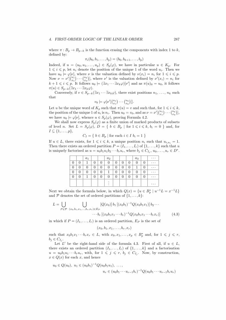
4. FIRST-ORDER LOGIC OF THE LINEAR ORDER 287
where π : Bp → Bp−k is the function erasing the components with index 1 to k,defined by:
πi(b0, b1, . . . , bp) = (b0, bk+1, . . . , bp)
Indeed, if u = (u0, u1, . . . , up) ∈ Sp(ϕ), we have in particular u ∈ Kp. For1 6 i 6 p, let ni denote the position of the unique 1 of the word ui. Then wehave u0 |= ϕ[ν], where ν is the valuation defined by ν(xi) = ni for 1 6 i 6 p.Now ν = ν′[
(n1
x1
)· · ·
(nk
xk
)], where ν′ is the valuation defined by ν′(xi) = ni for
k + 1 6 i 6 p. It follows u0 |= (∃x1 · · · ∃xkϕ)[ν′] and as π(u)0 = u0, it followsπ(u) ∈ Sp−k(∃x1 · · · ∃xkϕ).
Conversely, if v ∈ Sp−k(∃x1 · · · ∃xkϕ), there exist positions n1, . . . , nk suchthat
v0 |= ϕ[ν′[(n1
x1
)· · ·
(nk
xk
)]].
Let u be the unique word of Kp such that π(u) = v and such that, for 1 6 i 6 k,the position of the unique 1 of ui is ni. Then u0 = v0, and as ν = ν′[
(n1
x1
)· · ·
(nk
xk
)],
we have u0 |= ϕ[ν], whence u ∈ Sp(ϕ), proving Formula 4.2.We shall now express Sp(ϕ) as a finite union of marked products of subsets
of level n. Set L = Sp(ϕ), D = { b ∈ Bp | for 1 6 i 6 k, bi = 0 } and, forI ⊆ {1, . . . , p},
CI = { b ∈ Bp | for each i ∈ I bi = 1 }
If u ∈ L, there exists, for 1 6 i 6 k, a unique position ni such that ui,ni= 1.
Then there exists an ordered partition P = (I1, . . . , Ir) of {1, . . . , k} such that uis uniquely factorised as u = u0b1u1b2 · · · brur, where bj ∈ CIj , u0, . . . , ur ∈ D
∗.
a1 a2 a3 · · ·0 0 1 0 0 0 0 0 0 0 0 · · ·0 0 0 0 0 0 0 0 0 1 0 · · ·0 0 0 0 0 1 0 0 0 0 0 · · ·0 0 1 0 0 0 0 0 0 0 0 · · ·
... · · ·
Next we obtain the formula below, in which Q(x) = {u ∈ B∗p | u
−1L = x−1L}and P denotes the set of ordered partitions of {1, . . . , k}:
L =⋃
P∈P
⋃
(x0,b1,x1,...,br,xr)∈EP
[Q(x0)] b1 [(x0b1)−1Q(x0b1x1)] b2 · · ·
· · · br [(x0b1x1 · · · br)−1Q(x0b1x1 · · · brxr)] (4.3)
in which if P = (I1, . . . , Ir) is an ordered partition, EP is the set of
(x0, b1, x1, . . . , br, xr)
such that x0b1x1 · · · brxr ∈ L, with x0, x1, . . . , xp ∈ B∗p and, for 1 6 j 6 r,
bj ∈ CIj .Let L′ be the right-hand side of the formula 4.3. First of all, if u ∈ L,
there exists an ordered partition (I1, . . . , Ir) of {1, . . . , k} and a factorisationu = u0b1u1 · · · brur, with, for 1 6 j 6 r, bj ∈ CIj . Now, by construction,x ∈ Q(x) for each x, and hence
u0 ∈ Q(u0), u1 ∈ (u0b1)−1Q(u0b1u1), . . . ,
ur ∈ (u0b1 · · ·ur−1br)−1Q(u0b1 · · ·ur−1brur)

288 CHAPTER XVIII. AN EXCURSION INTO LOGIC
thereby establishing the inclusion L ⊆ L′. Conversely, if there exists an orderedpartition P of {1, . . . , k} and if
u ∈ [Q(x0)] b1 [(x0b1)−1Q(x0b1x1)] b2 · · ·
bk [(x0b1x1 · · · br)−1Q(x0b1x1 · · · brxr)]
for some (x0, b1, x1, . . . , bk, xr) ∈ EP , we have u = u0b1u1 · · · brur, with bj ∈ CIj
and
u0 ∈ Q(x0), u1 ∈ (x0b1)−1Q(x0b1x1), . . . ,
ur ∈ (x0b1x1 · · · br)−1Q(x0b1x1 · · · brxr)
Therefore, for 0 6 i 6 r, x0b1x1 · · · biui ∈ Q(x0b1x1 · · · bixi), whence
(x0b1x1 · · · biui)−1L = (x0b1x1 · · · bixi)
−1L
Next we show that x0b1x1 · · · bixibi+1ui+1 · · · brur ∈ L by induction on r−i. Fori = r, the result follows from the fact that (x0, b1, x1, . . . , br, xr) ∈ EP . Next, if
x0b1x1 · · · bixibi+1ui+1 · · · brur ∈ L
we have bi+1ui+1 · · · brur ∈ (x0b1x1 · · · bixi)−1L and hence
bi+1ui+1 · · · brur ∈ (x0b1x1 · · · biui)−1L
whence x0b1x1 · · · bi−1xi−1biui · · · brur ∈ L, allowing the induction. Conse-quently
u = u0b1u1 · · · brur ∈ L
and the inclusion L′ ⊆ L is proved.A second formula gives an expression of Q(x) in terms of quotients of L.
Q(x) = (⋂
y∈x−1L
Ly−1) − (⋃
y/∈x−1L
Ly−1) (4.4)
Let indeedQ′(x) be the right-hand side of (4.4). If u ∈ Q(x), then u−1L = x−1L.Therefore the following sequence of equivalences hold
y ∈ x−1L⇐⇒ y ∈ u−1L⇐⇒ uy ∈ L⇐⇒ u ∈ Ly−1
showing that Q(x) ⊆ Q′(x). Let now u ∈ Q′(x). If y ∈ x−1L, then u ∈ Ly−1
and hence uy ∈ L and y ∈ u−1L. Similarly, if y /∈ x−1L, then y /∈ u−1L.Therefore u−1L = x−1L and u ∈ Q(x), proving (4.4).
Since L is recognisable, Proposition III.4.17 shows that L has only finitelymany quotients on the right and on the left. It follows that only finitelymany unions and intersections occur in Formulas (4.3) and (4.4). Furthermore,Lemma 4.19 shows that all the quotients of L are of level n. Consequently,the subsets of the form Q(x) and their quotients are of level n. Formula 4.3now gives an expression of Sp(ϕ) as a finite union of products of the formX0b1X1 · · · brXr where bj ∈ CIj and the X0, . . . , Xr are level n subsets of D∗.By Formula 4.2, Sp−r(∃xi1 · · · ∃xirϕ) is thus a finite union of subsets of the formπ(X0b1X1b2 · · · brXr). Therefore, proving that Sp−r(∃xi1 · · · ∃xikϕ) is of level
XVIII.4. FIRST-ORDER LOGIC OF THE LINEAR ORDER 289
n+ 1/2, amounts to proving that if X is a subset of B∗p of level n contained in
D∗, then π(X) is a subset of B∗p−k of level n.
Let δ : Bp−k → Bp be the function defined by
δ(b0, . . . , bp−k) = (b0, 0, . . . , 0, b1, . . . , bp−k)
Then we have, for each subset X of D∗,
π(X) = δ−1(X)
Thus, it suffices to verify by induction that the subsets of level n [n+ 1/2] arestable under δ−1. For level 0, this follows from the formulas
δ−1(K(ε1, . . . , εp−k)) = K(0, . . . , 0, εk+1, . . . , εp)
δ−1(K(a, i, ε1, . . . , εp−k)) = K(a, k + i, 0, . . . , 0, εk+1, . . . , εp)
δ−1(K=(i, j, ε1, . . . , εp−k)) = K=(k + i, k + j, 0, . . . , 0, εk+1, . . . , εp)
δ−1(K=(i, j, ε1, . . . , εp−k)) = K<(k + i, k + j, 0, . . . , 0, εk+1, . . . , εp)
and from the fact that δ−1 commutes with the Boolean operations. This latterproperty also permits one to pass from level n+1/2 to level n+1 in the inductionstep. Passing from level n to level n+ 1/2, requires the formula
δ−1(X0b1X1 · · · bkXk) =⋃
c1∈δ−1(b1)
...
ck∈δ−1(bk)
δ−1(X0)c1δ−1(X1) · · · ckδ
−1(Xk)
which follows from the fact that δ is length preserving.
We can now conclude the second part of the proof of Theorem 4.17. Sincethe only variable-free formulas of BΣ0 are true and false, the only subsets ofA∗ definable by a formula of BΣ0[<] are ∅ and A
∗, which are indeed of level 0.By Lemma 4.20, for each formula ϕ of BΣ0[<], Lp(ϕ) is a subset of B∗
p oflevel 0. Suppose by induction that, for each formula ϕ of BΣn[<], Lp(ϕ) is asubset of B∗
p of level n. Consider the set ∆ of formulas ϕ such that, for eachp > 0, Lp(ϕ) is a subset of B∗
p of level n + 1/2. The set ∆ contains BΣn[<]by the induction hypothesis and, by Proposition 3.9, it is closed under finitedisjunction and finite conjunction. Finally, Lemma 4.21 shows that if ϕ ∈ ∆and if x1, . . . , xk are free variables of ϕ, then ∃x1 · · · ∃xkϕ ∈ ∆. Therefore∆ contains Σn+1[<] and each formula of Σn+1[<] defines a subset B∗
p of leveln+ 1/2.
To conclude, suppose by induction that for each formula ϕ of Σn+1[<], Lp(ϕ)is a subset of B∗
p of level n+1/2. The proof of Proposition 3.8 shows that Kp isof level 1 and thus Proposition 3.9 shows that for each formula ϕ of BΣn+1[<],Lp(ϕ) is a subset of B∗
p of level n+ 1.
290 CHAPTER XVIII. AN EXCURSION INTO LOGIC

Annex A
A transformation semigroup
We compute in this section the structure of a 4-generator transformation semi-group S. We compute successively the list of its elements, a presentation forit, its right and left Cayley graphs, its D-class structure and the lattice of itsidempotents.
∗ 1 1 2 3 4
a 2 3 4 0
b 3 1 4 0
c 2 1 4 3
a2 3 4 0 0
ab 1 4 0 0
ac 1 4 3 0
ba 4 2 0 0
b2 4 3 0 0
bc 4 2 3 0
ca 3 2 0 4
cb 1 3 0 4
a3 4 0 0 0
aba 2 0 0 0
ab2 3 0 0 0
abc 2 3 0 0
aca 2 0 4 0
acb 3 0 4 0
ba2 0 3 0 0
bab 0 1 0 0
bac 3 1 0 0
b2a 0 4 0 0
bca 0 3 4 0
bcb 0 1 4 0
cab 4 1 0 0
1 2 3 4
cac 4 1 0 3
cba 2 4 0 0
cbc 2 4 0 3
∗ a4 0 0 0 0
∗ bab 1 0 0 0
∗ cac 1 0 3 0
acbc 4 0 3 0
∗ baba 0 2 0 0
bcac 0 4 3 0
∗ bcbc 0 2 3 0
cabc 3 2 0 0
∗ caca 0 2 0 4
cacb 0 3 0 4
cbac 1 3 0 0
cbca 3 0 0 4
∗ cbcb 1 0 0 4
acbca 0 0 4 0
cacac 0 1 0 3
cacbc 0 4 0 3
cbcac 4 0 0 3
cbcbc 2 0 0 3
∗ acbcac 0 0 3 0
∗ cacbca 0 0 0 4
cacbcac 0 0 0 3
291
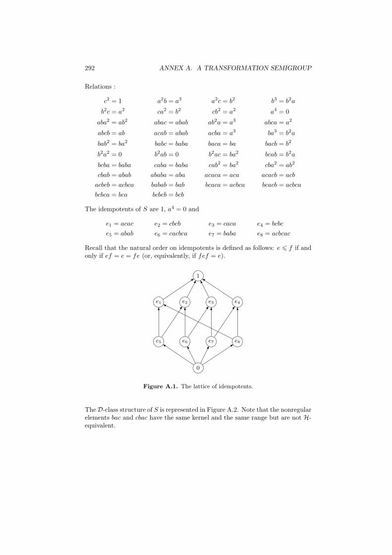
292 ANNEX A. A TRANSFORMATION SEMIGROUP
Relations :
c2 = 1 a2b = a3 a2c = b2 b3 = b2a
b2c = a2 ca2 = b2 cb2 = a2 a4 = 0
aba2 = ab2 abac = abab ab2a = a3 abca = a2
abcb = ab acab = abab acba = a3 ba3 = b2a
bab2 = ba2 babc = baba baca = ba bacb = b2
b2a2 = 0 b2ab = 0 b2ac = ba2 bcab = b2a
bcba = baba caba = baba cab2 = ba2 cba2 = ab2
cbab = abab ababa = aba acaca = aca acacb = acb
acbcb = acbca babab = bab bcaca = acbca bcacb = acbca
bcbca = bca bcbcb = bcb
The idempotents of S are 1, a4 = 0 and
e1 = acac e2 = cbcb e3 = caca e4 = bcbc
e5 = abab e6 = cacbca e7 = baba e8 = acbcac
Recall that the natural order on idempotents is defined as follows: e 6 f if andonly if ef = e = fe (or, equivalently, if fef = e).
1
e1 e2 e3 e4
e5 e6 e7 e8
0
Figure A.1. The lattice of idempotents.
TheD-class structure of S is represented in Figure A.2. Note that the nonregularelements bac and cbac have the same kernel and the same range but are not H-equivalent.

293
01234
0/1/2/3/4∗1, c
0234 0134
1/2/3/04 a ac
1/2/4/03 ca cac
1/2/3/04 bc b
1/2/4/03 cbc cb
013 024
1/3/024∗acac aca
2/4/013 cacac∗caca
034
acb acbc
cacb cacbc
1/2/034 bac ba
1/2/034 cbac cba
a2
b2
abc ab 1/2/034
cabc cab 1/2/034
bca bcac
cbca cbcac
034
∗bcbc bcb 2/3/014
cbcbc∗cbcb 1/4/023
023 014
01 02
1/0234∗abab aba
2/0134 bab∗baba
03 04
ab2 a3
ba2 b2a
∗acbcac acbca 3/0124
cacbcac∗cacbca 4/0123
0
01234∗0
Figure A.2. The D-class structure of S.

294 ANNEX A. A TRANSFORMATION SEMIGROUP
1
c
a
ac
ca
cac
b
bc
cb
cbc
aa
abba
bb aaa
aba
abb
abc
aca
acb
baa
bab
bac
bba
bca
bcb
cab cba
0
0
abab
acac
acbc
baba
bcac
bcbc
cabc
caca
cacb
cbac
cbca
cbcb
acbca
cacac
cacbc cbcac
cbcbc
acbcac
cacbca
cacbcac
ab
c
a
b
c
a
b
c
a b
ca, b
c
ab
c
a
b
c
ab
c
a, bc
ab
c
a
b
c
a
b
c
a, b
ca
b, c
a, b, c
a
b, c a
b
c
a, b
c
a, b, c
a, c
b
a, c
b
a, b
c
a, b
c
a
b
c
ab
c
a
b
c
ab
c
a
b
c
a, b, c
a, b, c
a, c
b
a, c
b
a, b
c
a
b, c
a, b
c
a
b, c
a
b, ca
b
c
a, b
c
a, c
b
a, b
c
a
b
c
a, b
c
a, c
b
a, b
c
a, b
c
a
b, c
a, b, c
a, b
c a, b, c
Figure A.3. The right Cayley graph of S. To avoid unesthetic crossinglines, the zero is represented twice in this diagram.

295
1
c
a
ac
ca
cac
b
bc
cb
cbc
aa
ab
ba
bb
aaa
aba
abb abc
aca
acb
baa
bab
bac
bba
bca
bcb
cab
cba
00abab
acac
acbc
baba
bcac
bcbc
cabc
caca
cacb
cbac
cbca
cbcb
acbca
cacac
cacbccbcac
cbcbc
acbcac
cacbca
cacbcac
ab
c
a
bc
a
b
c
a b
c
a
b
c
a
b
c
a
b
c
a
b
c
a
b
c
a
b
c
a
b
c
a
b
ca
b, c
a
b, c
a
b, c
a
b
c
a
b
c
a
b
c
a, c
b
a, c
ba
b
c
a, c
b
a
bc
a
bc
a
b
c
a
b
c
a
b
c
a
b
c
a, b, ca, b, c
a
b, c
a
b
c
a
b
c
a, c
b
a
bc
a
b c
a
b
c
a, c
b
a, c
b
a
b
c
a
b, c
a
b, c
a
b
c
a, c
b
a, c
ba
b, c
a
b, c
a
b
c
a, b, c
a, b, c
Figure A.4. The left Cayley graph of S. To avoid unesthetic crossinglines, the zero is represented twice in this diagram.
296 ANNEX A. A TRANSFORMATION SEMIGROUP

Bibliography
[1] J. Almeida, Residually finite congruences and quasi-regular subsets inuniform algebras, Portugal. Math. 46,3 (1989), 313–328.
[2] J. Almeida, Implicit operations on finite J -trivial semigroups and a con-jecture of I. Simon, J. Pure Appl. Algebra 69,3 (1991), 205–218.
[3] J. Almeida, Finite semigroups and universal algebra, World ScientificPublishing Co. Inc., River Edge, NJ, 1994. Translated from the 1992Portuguese original and revised by the author.
[4] J. Almeida, Profinite semigroups and applications, in Structural theoryof automata, semigroups, and universal algebra, pp. 1–45, NATO Sci. Ser.II Math. Phys. Chem. vol. 207, Springer, Dordrecht, 2005. Notes takenby Alfredo Costa.
[5] J. Almeida and M. V. Volkov, Profinite identities for finite semigroupswhose subgroups belong to a given pseudovariety, J. Algebra Appl. 2,2(2003), 137–163.
[6] J. Almeida and P. Weil, Relatively free profinite monoids: an intro-duction and examples, in NATO Advanced Study Institute Semigroups,Formal Languages and Groups, J. Fountain (ed.), vol. 466, pp. 73–117,Kluwer Academic Publishers, 1995.
[7] M. Arfi, Polynomial operations on rational languages, in STACS 87(Passau, 1987), pp. 198–206, Lecture Notes in Comput. Sci. vol. 247,Springer, Berlin, 1987.
[8] M. Arfi, Operations polynomiales et hierarchies de concatenation, The-oret. Comput. Sci. 91,1 (1991), 71–84.
[9] B. Banaschewski, The Birkhoff theorem for varieties of finite algebras,Algebra Universalis 17,3 (1983), 360–368.
[10] M.-P. Beal, O. Carton and C. Reutenauer, Cyclic languages andstrongly cyclic languages, in STACS 96 (Grenoble, 1996), pp. 49–59, Lect.Notes Comp. Sci. vol. 1046, Springer, Berlin, 1996.
[11] J. Berstel, Transductions and context-free languages, Teubner, 1979.
[12] J. Berstel, D. Perrin and C. Reutenauer, Codes and Automata,Encyclopedia of Mathematics and its Applications vol. 129, CambridgeUniversity Press, 2009. 634 pages.
297

298 BIBLIOGRAPHY
[13] G. Birkhoff, On the structure of abstract algebras, Proc. CambridgePhil. Soc. 31 (1935), 433–454.
[14] G. Birkhoff, Moore-Smith convergence in general topology, Annals ofMathematics 38 (1937), 39–56.
[15] B. Borchert, D. Kuske and F. Stephan, On existentially first-orderdefinable languages and their relation to NP, in Automata, languages andprogramming (Aalborg, 1998), pp. 17–28, Lecture Notes in Comput. Sci.vol. 1443, Springer, Berlin, 1998.
[16] M. J. Branco and J.-E. Pin, Equations for the polynomial closure, inICALP 2009, Part II, S. Albers and W. Thomas (eds.), pp. 115–126, Lect.Notes Comp. Sci. vol. 5556, Springer, Berlin, 2009.
[17] J. Brzozowski, K. Culik and A. Gabrielan, Classification of non-counting events, J. Comput. Syst. Sci. 5 (1971), 41–53.
[18] J. A. Brzozowski, Hierarchies of Aperiodic Languages, Theoret. Infor-matics Appl. 10,2 (1976), 33–49.
[19] J. A. Brzozowski and F. E. Fich, Languages of R-Trivial Monoids, J.Comput. Syst. Sci. 20,1 (1980), 32–49.
[20] J. A. Brzozowski and R. Knast, The dot-depth hierarchy of star-freelanguages is infinite, J. Comput. System Sci. 16,1 (1978), 37–55.
[21] J. A. Brzozowski and I. Simon, Characterizations of locally testableevents, Discrete Math. 4 (1973), 243–271.
[22] J. R. Buchi, Weak second-order arithmetic and finite automata, Z. Math.Logik und Grundl. Math. 6 (1960), 66–92.
[23] J. R. Buchi, On a decision method in restricted second order arithmetic,in Logic, Methodology and Philosophy of Science (Proc. 1960 Internat.Congr .), pp. 1–11, Stanford Univ. Press, Stanford, Calif., 1962.
[24] J. Carroll and D. Long, Theory of finite automata with an intro-duction to formal languages, Prentice-Hall, Inc., Upper Saddle River, NJ,USA, 1989.
[25] O. Carton, Langages formels, calculabilite et complexite, Vuibert, 2008.
[26] O. Carton, J.-E. Pin and X. Soler-Escriva, Languages Recog-nized by Finite Supersoluble Groups, Journal of Automata, Languagesand Combinatorics 14,2 (2009), 149–161.
[27] J. Chalopin and H. Leung, On factorization forests of finite height,Theoret. Comput. Sci. 310,1-3 (2004), 489–499.
[28] A. H. Clifford and G. B. Preston, The Algebraic Theory of Semi-groups, vol. 1, Amer. Math. Soc., 1961.
[29] A. H. Clifford and G. B. Preston, The Algebraic Theory of Semi-groups, vol. 2, Amer. Math. Soc., 1967.

BIBLIOGRAPHY 299
[30] J. Cohen, D. Perrin and J.-E. Pin, On the expressive power of tem-poral logic, J. Comput. System Sci. 46,3 (1993), 271–294.
[31] R. S. Cohen and J. A. Brzozowski, On star-free events, in Proc.Hawaii Int. Conf. on System Science, B. K. Kinariwala and F. F. Kuo(eds.), pp. 1–4, University of Hawaii Press, Honolulu, HI, 1968.
[32] T. Colcombet, A combinatorial theorem for trees: applications tomonadic logic and infinite structures, in Automata, languages and pro-gramming, pp. 901–912, Lect. Notes Comp. Sci. vol. 4596, Springer, Berlin,2007.
[33] T. Colcombet, Factorisation Forests for Infinite Words, in Fundamentalsof Computation Theory, 16th International Symposium, FCT 2007, Bu-dapest, Hungary, August 27-30, 2007, Proceedings, E. Csuhaj-Varju andZ. Esik (eds.), pp. 226–237, Lect. Notes Comp. Sci. vol. 4639, Springer,Berlin, 2007.
[34] J. H. Conway, Regular Algebra and Finite Machines, Chapman and Hall,London, 1971.
[35] D. M. Davenport, On power commutative semigroups, Semigroup Fo-rum 44,1 (1992), 9–20.
[36] A. De Luca and S. Varricchio, Finiteness and Regularity in Semi-groups and Formal Languages, Springer-Verlag, 1999.
[37] V. Diekert and P. Gastin, Pure future local temporal logics are ex-pressively complete for Mazurkiewicz traces, Inform. and Comput. 204,11(2006), 1597–1619. Conference version in LATIN 2004, LNCS 2976, 170–182, 2004.
[38] V. Diekert and M. Kufleitner, A survey on the local divisor tech-nique, Theoret. Comput. Sci. 610,part A (2016), 13–23.
[39] S. Eilenberg, Automata, languages, and machines. Vol. A, AcademicPress [A subsidiary of Harcourt Brace Jovanovich, Publishers], New York,1974. Pure and Applied Mathematics, Vol. 58.
[40] S. Eilenberg, Automata, languages, and machines. Vol. B, AcademicPress [Harcourt Brace Jovanovich Publishers], New York, 1976. With twochapters (“Depth decomposition theorem” and “Complexity of semigroupsand morphisms”) by Bret Tilson, Pure and Applied Mathematics, Vol. 59.
[41] C. C. Elgot, Decision problems of finite automata design and relatedarithmetics, Trans. Amer. Math. Soc. 98 (1961), 21–51.
[42] Z. Esik, Extended temporal logic on finite words and wreath productsof monoids with distinguished generators, in DLT 2002, Kyoto, Japan,M. E. A. Ito (ed.), Berlin, 2002, pp. 43–58, Lect. Notes Comp. Sci. n 2450,Springer.
[43] Z. Esik and M. Ito, Temporal logic with cyclic counting and the degreeof aperiodicity of finite automata, Acta Cybernetica 16 (2003), 1–28.

300 BIBLIOGRAPHY
[44] Z. Esik and K. G. Larsen, Regular languages definable by Lindstromquantifiers, Theoret. Informatics Appl. 37 (2003), 179–241.
[45] M. Gehrke, S. Grigorieff and J.-E. Pin, Duality and equationaltheory of regular languages, in ICALP 2008, Part II, L. A. et al. (ed.),Berlin, 2008, pp. 246–257, Lect. Notes Comp. Sci. vol. 5126, Springer.
[46] S. Ginsburg and E. H. Spanier, Bounded ALGOL-like languages,Trans. Amer. Math. Soc. 113 (1964), 333–368.
[47] S. Ginsburg and E. H. Spanier, Bounded regular sets, Proc. Amer.Math. Soc. 17 (1966), 1043–1049.
[48] S. Ginsburg and E. H. Spanier, Semigroups, Presburger formulas, andlanguages, Pacific J. Math. 16 (1966), 285–296.
[49] A. Ginzburg, Algebraic theory of automata, Academic Press, New York,1968.
[50] C. Glaßer and H. Schmitz, Languages of dot-depth 3/2, in STACS2000 (Lille), pp. 555–566, Lecture Notes in Comput. Sci. vol. 1770,Springer, Berlin, 2000.
[51] R. Graham, On finite 0-simple semigroups and graph theory, Math. Syst.Theory 2 (1968), 325–339.
[52] J. A. Green, On the structure of semigroups, Ann. of Math. (2) 54(1951), 163–172.
[53] P. A. Grillet, Semigroups, An Introduction to the Structure Theory,Marcel Dekker, Inc., New York, 1995.
[54] M. Hall, A Topology for free groups and related groups, Annals of Math-ematics 52 (1950), 127–139.
[55] K. Henckell and J.-E. Pin, Ordered monoids and J -trivial monoids,in Algorithmic problems in groups and semigroups (Lincoln, NE, 1998),pp. 121–137, Trends Math.
[56] K. Henckell and J. Rhodes, The theorem of Knast, the PG = BG andtype-II conjectures, in Monoids and semigroups with applications (Berke-ley, CA, 1989), pp. 453–463, World Sci. Publ., River Edge, NJ, 1991.
[57] J. B. Hickey, Semigroups under a sandwich operation, Proc. EdinburghMath. Soc. (2) 26,3 (1983), 371–382.
[58] Higgins, Techniques of Semigroup Theory, World Scientific, 1999.
[59] P. M. Higgins, A new proof of Schutzenberger’s theorem, Internat. J.Algebra Comput. 10,2 (2000), 217–220.
[60] J. Hopcroft, R. Motwani and J. D. Ullman, Introduction to au-tomata theory, languages, and computation, Addison-Wesley, Boston,ed. 2nd, 2001.
BIBLIOGRAPHY 301
[61] J. Hopcroft and J. D. Ullman, Introduction to Automata Theory,Languages and Computation, Addison Wesley, 1979.
[62] J. M. Howie, An Introduction to Semigroup Theory, Academic Press,1976.
[63] J. M. Howie, Automata and Languages, Clarendon Press, 1991.
[64] J. M. Howie, Fundamentals of semigroup theory, London MathematicalSociety Monographs. New Series vol. 12, The Clarendon Press OxfordUniversity Press, New York, 1995. Oxford Science Publications.
[65] L. (http://math.stackexchange.com/users/17760/lubin), Refer-ence request for tricky problem in elementary group theory. Mathemat-ics Stack Exchange. URL:http://math.stackexchange.com/q/253514 (ver-sion: 2016-02-29).
[66] S. C. Kleene, Representation of events in nerve nets and finite automata,in Automata studies, pp. 3–41, Princeton University Press, Princeton, N.J., 1956. Annals of mathematics studies, no. 34.
[67] O. Klıma, Piecewise testable languages via combinatorics on words, Dis-crete Math. 311,20 (2011), 2124–2127.
[68] R. Knast, A semigroup characterization of dot-depth one languages,RAIRO Inform. Theor. 17,4 (1983), 321–330.
[69] R. Knast, Some theorems on graph congruences, RAIRO Inform. Theor.17,4 (1983), 331–342.
[70] D. Krob, Complete sets of B-rational identities, Theoret. Comp. Sci. 89(1991), 207–343.
[71] M. Kufleitner, The Height of Factorization Forests, in Mathemati-cal Foundations of Computer Science 2008, 33rd International Sympo-sium, MFCS 2008, Torun, Poland, August 25-29, 2008, Proceedings,E. Ochmanski and J. Tyszkiewicz (eds.), pp. 443–454, Lect. Notes Comp.Sci. vol. 5162, Springer, Berlin, 2008.
[72] M. Kunc, Equational description of pseudovarieties of homomorphisms,Theoretical Informatics and Applications 37 (2003), 243–254.
[73] G. Lallement, Semigroups and Combinatorial Applications, Wiley andSons, 1979.
[74] M. V. Lawson, Finite Automata, CRC Press, 2003.
[75] M. Lothaire, Combinatorics on Words, Encyclopedia of Mathematicsand its Applications vol. 17, Cambridge University Press, 1983.
[76] M. Lothaire, Combinatorics on words, Cambridge Mathematical Li-brary, Cambridge University Press, Cambridge, 1997. With a forewordby Roger Lyndon and a preface by Dominique Perrin, Corrected reprintof the 1983 original, with a new preface by Perrin.

302 BIBLIOGRAPHY
[77] S. Margolis and J.-E. Pin, Products of group languages, in FCT,Berlin, 1985, pp. 285–299, Lect. Notes Comp. Sci. n 199, Springer.
[78] Mascle, Torsion Matrix Semigroups and Recognizable Transductions, inAutomata, Languages and Programming, Kott (ed.), Berlin, 1986, pp. 244–253, Lect. Notes Comp. Sci., Springer.
[79] R. McNaughton, Algebraic decision procedures for local testability,Math. Systems Theory 8,1 (1974), 60–76.
[80] R. McNaughton and S. Papert, Counter-free automata, The M.I.T.Press, Cambridge, Mass.-London, 1971. With an appendix by WilliamHenneman, M.I.T. Research Monograph, No. 65.
[81] A. R. Meyer, A note on star-free events, J. Assoc. Comput. Mach. 16(1969), 220–225.
[82] M. Morse and G. A. Hedlund, Unending chess, symbolic dynamicsand a problem in semigroups, Duke Math. J. 11 (1944), 1–7.
[83] G. Paun and A. Salomaa, Thin and slender languages, Discrete Appl.Math. 61,3 (1995), 257–270.
[84] M. Perles, M. Rabin and E. Shamir, The theory of definite automata,IEEE Trans. Electron. Comput. 12 (1963), 233–243.
[85] D. Perrin, Finite automata, in Handbook of theoretical computer science,Vol. B, pp. 1–57, Elsevier, Amsterdam, 1990.
[86] D. Perrin and J.-E. Pin, Infinite Words, Pure and Applied Mathematicsvol. 141, Elsevier, 2004. ISBN 0-12-532111-2.
[87] M. Petrich, Inverse Semigroups, Wiley and Sons, 1984.
[88] S. Piccard, Sur les fonctions definies dans les ensembles finis quelcon-ques, Fundam. Math. 24 (1935), 298–301.
[89] J.-E. Pin, Proprietes syntactiques du produit non ambigu, in 7th ICALP,Berlin, 1980, pp. 483–499, Lect. Notes Comp. Sci. n 85, Springer.
[90] J.-E. Pin, Hierarchies de concatenation, RAIRO Inform. Theor. 18,1(1984), 23–46.
[91] J.-E. Pin, Varieties of formal languages, Plenum Publishing Corp., NewYork, 1986. With a preface by M.-P. Schutzenberger, Translated from theFrench by A. Howie.
[92] J.-E. Pin, A property of the Schutzenberger product, Semigroup Forum35 (1987), 53–62.
[93] J.-E. Pin, Finite semigroups and recognizable languages: an introduc-tion, in Semigroups, formal languages and groups (York, 1993), pp. 1–32,Kluwer Acad. Publ., Dordrecht, 1995.
[94] J.-E. Pin, A variety theorem without complementation, Russian Mathe-matics (Iz. VUZ) 39 (1995), 80–90.

BIBLIOGRAPHY 303
[95] J.-E. Pin, The expressive power of existential first order sentences ofBuchi’s sequential calculus, in Automata, languages and programming(Paderborn, 1996), pp. 300–311, Lecture Notes in Comput. Sci. vol. 1099,Springer, Berlin, 1996.
[96] J.-E. Pin, Logic, Semigroups and Automata on Words, Annals of Math-ematics and Artificial Intelligence 16 (1996), 343–384.
[97] J.-E. Pin, Polynomial closure of group languages and open sets of the Halltopology, Theoret. Comput. Sci. 169 (1996), 185–200. Journal version ofthe article of ICALP 1994.
[98] J.-E. Pin, Syntactic semigroups, in Handbook of formal languages,G. Rozenberg and A. Salomaa (eds.), vol. 1, ch. 10, pp. 679–746, SpringerVerlag, 1997.
[99] J.-E. Pin, Bridges for concatenation hierarchies, in 25th ICALP, pp. 431–442, Lect. Notes Comp. Sci. n 1443, Springer, Berlin, 1998.
[100] J.-E. Pin, Logic On Words, in Current Trends in Theoretical ComputerScience, Entering the 21st Century, G. R. G. Paun and A. Salomaa (eds.),pp. 254–273, Word Scientific, 2001.
[101] J.-E. Pin, Algebraic tools for the concatenation product, Theoret. Com-put. Sci. 292 (2003), 317–342.
[102] J.-E. Pin, The expressive power of existential first order sentences ofBuchi’s sequential calculus, Discrete Mathematics 291 (2005), 155–174.
[103] J.-E. Pin, Profinite methods in automata theory, in 26th Interna-tional Symposium on Theoretical Aspects of Computer Science (STACS2009), S. Albers (ed.), pp. 31–50, Internationales Begegnungs- UndForschungszentrum fur Informatik (IBFI), Schloss Dagstuhl, Germany,Dagstuhl, Germany, 2009.
[104] J.-E. Pin, A. Pinguet and P. Weil, Ordered categories and orderedsemigroups, Communications in Algebra 30 (2002), 5651–5675.
[105] J.-E. Pin and H. Straubing, Monoids of upper triangular matrices, inSemigroups (Szeged, 1981), pp. 259–272, Colloq. Math. Soc. Janos Bolyaivol. 39, North-Holland, Amsterdam, 1985.
[106] J.-E. Pin and H. Straubing, Some results on C-varieties, Theoret. In-formatics Appl. 39 (2005), 239–262.
[107] J.-E. Pin, H. Straubing and D. Therien, Some results on the gen-eralized star-height problem, Information and Computation 101 (1992),219–250.
[108] J.-E. Pin and P. Weil, Polynomial closure and unambiguous product,in 22th ICALP, Berlin, 1995, pp. 348–359, Lect. Notes Comp. Sci. n 944,Springer.
[109] J.-E. Pin and P. Weil, Profinite semigroups, Mal’cev products andidentities, J. of Algebra 182 (1996), 604–626.

304 BIBLIOGRAPHY
[110] J.-E. Pin and P. Weil, A Reiterman theorem for pseudovarieties offinite first-order structures, Algebra Universalis 35 (1996), 577–595.
[111] J.-E. Pin and P. Weil, Polynomial closure and unambiguous product,Theory Comput. Systems 30 (1997), 1–39.
[112] J.-E. Pin and P. Weil, A conjecture on the concatenation product, ITA35 (2001), 597–618.
[113] J.-E. Pin and P. Weil, Semidirect products of ordered semigroups,Communications in Algebra 30 (2002), 149–169.
[114] J.-E. Pin and P. Weil, The wreath product principle for ordered semi-groups, Communications in Algebra 30 (2002), 5677–5713.
[115] N. Pippenger, Regular languages and Stone duality, Theory Comput.Syst. 30,2 (1997), 121–134.
[116] T. Place, Separating Regular Languages with Two Quantifier Alter-nations, in 30th Annual ACM/IEEE Symposium on Logic in ComputerScience (LICS 2015), pp. 202–213, IEEE, 2015.
[117] T. Place, L. Van Rooijen and M. Zeitoun, Separating regular lan-guages by locally testable and locally threshold testable languages, in 33ndInternational Conference on Foundations of Software Technology and The-oretical Computer Science, pp. 363–375, LIPIcs. Leibniz Int. Proc. Inform.vol. 24, Schloss Dagstuhl. Leibniz-Zent. Inform., Wadern, 2013.
[118] T. Place, L. Van Rooijen and M. Zeitoun, Separating regular lan-guages by piecewise testable and unambiguous languages, in Mathemati-cal foundations of computer science 2013, pp. 729–740, Lect. Notes Comp.Sci. vol. 8087, Springer, Heidelberg, 2013.
[119] T. Place, L. Van Rooijen and M. Zeitoun, On separation by locallytestable and locally threshold testable languages, Log. Methods Comput.Sci. 10,3 (2014), 3:24, 28.
[120] T. Place and M. Zeitoun, Going higher in the first-order quantifieralternation hierarchy on words, in Automata, languages, and program-ming. Part II, pp. 342–353, Lect. Notes Comp. Sci. vol. 8573, Springer,Heidelberg, 2014.
[121] T. Place and M. Zeitoun, Separating regular languages with first-order logic, in Joint Meeting of the Twenty-Third EACSL Annual Con-ference on Computer Science Logic (CSL) and the Twenty-Ninth AnnualACM/IEEE Symposium on Logic in Computer Science (LICS), CSL-LICS’14, Vienna, Austria, July 14 - 18, 2014, T. A. Henzinger and D. Miller(eds.), pp. 75:1–75:10, ACM, 2014.
[122] T. Place and M. Zeitoun, Separation and the Successor Relation, in32nd International Symposium on Theoretical Aspects of Computer Sci-ence, STACS 2015, March 4-7, 2015, Garching, Germany, E. W. Mayrand N. Ollinger (eds.), pp. 662–675, LIPIcs vol. 30, Schloss Dagstuhl -Leibniz-Zentrum Fuer Informatik, 2015.
BIBLIOGRAPHY 305
[123] L. Polak, Syntactic semiring of a language, in MFCS 2001, pp. 611–620,Lect. Notes Comp. Sci. vol. 2136, Springer, Berlin, 2001.
[124] M. O. Rabin and D. Scott, Finite automata and their decision prob-lems, Rap. Tech., IBM J. Res. and Develop., 1959. ”Reprinted in Sequen-tial Machines, E. F. Moore (ed.), Addison-Wesley, Reading, Massachus-setts, (1964), 63–91.”.
[125] N. R. Reilly and S. Zhang, Decomposition of the lattice of pseudova-rieties of finite semigroups induced by bands, Algebra Universalis 44,3-4(2000), 217–239.
[126] J. Reiterman, The Birkhoff theorem for finite algebras, Algebra Univer-salis 14,1 (1982), 1–10.
[127] C. Reutenauer, Une topologie du monoıde libre, Semigroup Forum 18,1(1979), 33–49.
[128] C. Reutenauer, Sur mon article: “Une topologie du monoıde libre”[Semigroup Forum 18 (1979), no. 1, 33–49; MR 80j:20075], SemigroupForum 22,1 (1981), 93–95.
[129] J. Rhodes and B. Steinberg, The q-theory of finite semigroups,Springer Monographs in Mathematics, Springer, New York, 2009.
[130] J. Sakarovitch, Elements de theorie des automates, Vuibert, 2003.
[131] J. Sakarovitch, Elements of automata theory, Cambridge UniversityPress, Cambridge, 2009. Translated from the 2003 French original byReuben Thomas.
[132] A. Salomaa, Computation and automata, Encyclopedia of Mathemat-ics and its Applications vol. 25, Cambridge University Press, Cambridge,1985. With a foreword by Grzegorz Rozenberg.
[133] M. P. Schutzenberger, Une theorie algebrique du codage,Seminaire Dubreil. Algebre et theorie des nombres 9 (1955-1956), 1–24.http://eudml.org/doc/111094.
[134] M.-P. Schutzenberger, On finite monoids having only trivial sub-groups, Information and Control 8 (1965), 190–194.
[135] C. Selmi, Strongly locally testable semigroups with commuting idempo-tents and related languages, Theor. Inform. Appl. 33,1 (1999), 47–57.
[136] I. Simon, Hierarchies of Events with Dot-Depth One, PhD thesis, Univer-sity of Waterloo, Waterloo, Ontario, Canada, 1972.
[137] I. Simon, Piecewise testable events, in Proc. 2nd GI Conf., H. Brackage(ed.), pp. 214–222, Lecture Notes in Comp. Sci. vol. 33, Springer Verlag,Berlin, Heidelberg, New York, 1975.
[138] I. Simon, Limited Subsets of a Free Monoid, in Proc. 19th Annual Sym-posium on Foundations of Computer Science, Piscataway, N.J., 1978,pp. 143–150, IEEE.
306 BIBLIOGRAPHY
[139] I. Simon, Properties of factorization forests, in Formal properties of fi-nite automata and applications, Ramatuelle, France, May 23-27, 1988,Proceedings, pp. 65–72, Lect. Notes Comp. Sci. vol. 386, Springer, Berlin,1989.
[140] I. Simon, Factorization forests of finite height, Theoret. Comput. Sci. 72,1(1990), 65–94.
[141] I. Simon, A short proof of the factorization forest theorem, in Tree au-tomata and languages (Le Touquet, 1990), pp. 433–438, Stud. Comput.Sci. Artificial Intelligence vol. 10, North-Holland, Amsterdam, 1992.
[142] M. Stone, The theory of representations for Boolean algebras, Trans.Amer. Math. Soc. 40 (1936), 37–111.
[143] M. H. Stone, Applications of the theory of Boolean rings to generaltopology, Trans. Amer. Math. Soc. 41,3 (1937), 375–481.
[144] M. H. Stone, The representation of Boolean algebras, Bull. Amer. Math.Soc. 44,12 (1938), 807–816.
[145] H. Straubing, Aperiodic homomorphisms and the concatenation prod-uct of recognizable sets, J. Pure Appl. Algebra 15,3 (1979), 319–327.
[146] H. Straubing, Families of recognizable sets corresponding to certainvarieties of finite monoids, J. Pure Appl. Algebra 15,3 (1979), 305–318.
[147] H. Straubing, A generalization of the Schutzenberger product of finitemonoids, Theoret. Comput. Sci. 13,2 (1981), 137–150.
[148] H. Straubing, Relational morphisms and operations on recognizablesets, RAIRO Inf. Theor. 15 (1981), 149–159.
[149] H. Straubing, Finite semigroup varieties of the form V ∗ D, J. PureAppl. Algebra 36,1 (1985), 53–94.
[150] H. Straubing, Semigroups and languages of dot-depth two, Theoret.Comput. Sci. 58,1-3 (1988), 361–378. Thirteenth International Collo-quium on Automata, Languages and Programming (Rennes, 1986).
[151] H. Straubing, The wreath product and its applications, in Formal prop-erties of finite automata and applications (Ramatuelle, 1988), pp. 15–24,Lecture Notes in Comput. Sci. vol. 386, Springer, Berlin, 1989.
[152] H. Straubing, Finite automata, formal logic, and circuit complexity,Birkhauser Boston Inc., Boston, MA, 1994.
[153] H. Straubing, On logical descriptions of regular languages, in LATIN2002, Berlin, 2002, pp. 528–538, Lect. Notes Comp. Sci. n 2286, Springer.
[154] H. Straubing and D. Therien, Partially ordered finite monoids and atheorem of I. Simon, J. Algebra 119,2 (1988), 393–399.
[155] H. Straubing and P. Weil, On a conjecture concerning dot-depth twolanguages, Theoret. Comput. Sci. 104,2 (1992), 161–183.
BIBLIOGRAPHY 307
[156] A. Szilard, S. Yu, K. Zhang and J. Shallit, Characterizing regu-lar languages with polynomial densities, in Mathematical foundations ofcomputer science 1992 (Prague, 1992), pp. 494–503, Lect. Notes Comp.Sci. vol. 629, Springer, Berlin, 1992.
[157] D. Therien, Classification of finite monoids: the language approach,Theoret. Comput. Sci. 14,2 ang. (1981), 195–208.
[158] W. Thomas, Classifying regular events in symbolic logic, J. Comput.System Sci. 25,3 (1982), 360–376.
[159] A. Thue, Uber unendliche Zeichenreihen, Norske Vid. Selsk. Skr. I Math-Nat. Kl. 7 (1906), 1–22.
[160] A. Thue, Uber die gegenseitige Loge gleicher Teile gewisser Zeichenrei-hen, Norske Vid. Selsk. Skr. I Math-Nat. Kl. Chris. 1 (1912), 1–67.
[161] B. Tilson, On the complexity of finite semigroups, J. Pure Appl. Algebra5 (1974), 187–208.
[162] P. Weil, Some results on the dot-depth hierarchy, Semigroup Forum 46,3(1993), 352–370.
[163] P. Weil, Profinite methods in semigroup theory, Int. J. Alg. Comput. 12(2002), 137–178.
[164] Th. Wilke, Classifying discrete Temporal Properties, in STACS’99,C. Meinel (ed.), Trier, Germany, 1999, pp. 32–46, Lecture Notes in Com-put. Sci. vol. 1563, Springer.
[165] S. Yu, Regular languages, in Handbook of language theory, G. Rozenbergand A. Salomaa (eds.), vol. 1, ch. 2, pp. 679–746, Springer, 1997.

Index of Notation
2E , 16J , 956L, 956R, 951, 175
A, 153A∗, 132
B, 17B(1, 2), 264B1
2 , 16B2, 15B(I, J), 15Bn, 15BΣn, 275
Com, 152CS, 151
D, 149D, 98DA, 156DS, 154
E, 12
FO, 270
G, 152Gcom, 152GL2(Z), 16Gp, 152GS, 159
H, 96
J, 153J , 96J1, 153J−1, 157
J+1, 157
J−, 157J+, 157
K, 149
L, 153L, 96L1, 154LG, 151L1, 151ℓ1, 149LJ+, 157
MSO, 272
N , 17n, 26N, 149N−, 157N+, 157
P(E), 1P(M), 17Πn, 274
Q, 16
R, 153R, 16R, 96R1, 154r1, 149
Σn, 274
U+1 , 16
Un, 16Un, 16
Xc, 1
Z, 16
308
Index
accessible, 41, 45action, 25
faithful, 25addition, 11alphabet, 28aperiodic, 152, 153assignment, 272associative, 11automata
equivalent, 41automaton, 40
accessible, 45coaccessible, 45complete, 45deterministic, 43extended, 65extensive, 180flower, 239local, 58minimal, 54minimal accessible, 54Nerode, 53standard, 46trim, 45
B12 , 16
bandrectangular, 111
basis for a topology, 128Boolean operations, 1, 36
positive, 1bounded occurrence, 271
cancellative, 13semigroup, 13
Cauchy sequence, 129Cayley graph, 28chain, 9class
of recognisable languages, 165
closure, 127coaccessible, 41, 45coarser, 8cofinite, 182colouring, 31commutative, 11compact, 129completion, 129composition, 2concatenation, 28congruence, 90
generated by, 23nuclear, 23ordered monoid, 25Rees, 22semigroup, 22syntactic, 23, 86, 91
conjugate, 104constant map, 245content, 210continuous, 128cover, 27, 222
D-class, 98full, 113
decidable, 67degree, 221dense, 127disjunctive normal form, 274division, 19
of transformation semigroups,27
domain, 2, 272, 276
existential, 275exponent, 31extensive, 216
factor, 35left, 35
309

310 INDEX
right, 36factorisation
canonical, 228factorisation forest, 32finitely generated, 27, 75fixed-point-free, 26formula
atomic, 270second-order, 272
first-order, 270logically equivalent, 274second-order, 272
freemonoid, 28occurrence, 271profinite monoid, 132semigroup, 28
fully recognising, 75function, 2
bijective, 3extensive, 182injective, 3inverse, 4surjective, 3total, 2
graphof a relational morphism, 227
Green’s lemma, 100group, 13
generated by, 27in a semigroup, 18right, 124structure, 107symmetric, 26
group language, 93
H-class, 96Hausdorff, 128height function, 224hierarchy
logical, 283homeomorphism, 128
uniform, 129
ideal, 200-minimal, 21generated by, 21left, 20minimal, 21
principal, 21right, 20shuffle, 213
idempotent, 12identity, 11, 159
element, 11explicit, 145left, 12partial, 229right, 12
image, 3index, 30injective
relational morphism, 229inverse, 13, 14, 103
group, 13of a relation, 1semigroup, 13weak, 103
isometry, 129isomorphic, 18isomorphism, 18
J -class, 96J -trivial, 106
L-class, 96L-trivial, 106label, 41language, 35, 36
local, 56of the linear order, 276of the successor, 277piecewise testable, 214recognisable, 41recognised, 41simple, 213
lattice of languagesclosed under quotients, 164
length, 29letters, 28lifted, 116limit, 128linear
expression, 59local
automaton, 58language, 56
locally, 249group, 151
INDEX 311
trivial, 150, 249locally V, 159locally finite
variety, 145, 175logic
first-order, 269monadicsecond-order, 272weak, 274
second-order, 272logical symbol, 270
Mal’cev product, 235mapping, 2metric, 128model, 276monogenic, 27monoid, 11
bicyclic, 16free, 28free pro-V, 143generated by, 27inverse, 124separates, 142syntactic, 86, 91transition, 84
morphismfully recognising, 75group, 17length-decreasing, 167length-multiplying, 167length-preserving, 167monoid, 17non-erasing, 167of ordered monoids, 17recognising, 75semigroup, 17semiring, 18
multiplication, 11
Nerode equivalence, 55normal, 250null
D-class, 105semigroup, 12
occurrence, 28ω-term, 135open
ε-ball, 128
operationbinary, 11
order, 8natural, 97partial, 8prefix, 36shortlex, 36
order preserving, 216ordered automaton, 89Ordered monoids, 14
path, 41accepting, 41end, 41final, 41initial, 41length, 41origin, 41successful, 41
period, 30permutation, 25plus, 73polynomial closure, 221positive
stream, 165variety, 167
positive +-variety, 171prefix, 35prenex normal form, 275preorder
generated by a set, 8presentation, 29product, 1, 11, 20, 28, 36
of ideals, 21of transformation semigroups,
26unambiguous, 236
profiniteidentity, 145monoid, 132
profinite C-identity, 167profinite identity, 165, 168pumping lemma, 42pure, 238
quantifier, 270quotient, 19
left, 37, 78
R-class, 96

312 INDEX
R-trivial, 106range, 3rank, 34, 118rational, 38rational expression, 39
linear, 59value, 40
recognisable, 78refinement, 127regular, 38, 105
D-class, 105semigroup, 105
relation, 1antisymmetric, 8coarser, 8equivalence, 8injective, 4preorder, 8reflexive, 8surjective, 4symmetric, 8thinner, 8transitive, 8universal, 8
relational morphism, 227aperiodic, 230locally trivial, 230
reversal, 35right-zero
semigroup, 26ring, 14
sandwich matrix, 107saturate, 76semigroup, 11
0-simple, 22A-generated, 27Brandt, 107aperiodic, 107
commutative, 11compact, 130dual, 11flower, 240free, 28generated by, 27left 0-simple, 22left simple, 22left zero, 15local, 34n, 26
nilpotent, 148order, 11ordered, 14Reeswith zero, 107
Rees matrix, 107right 0-simple, 22right simple, 22simple, 22syntactic, 23topological, 130transformation, 25
semilattice, 153semilinear, 74semiring, 14
Boolean, 17sentence, 271set
closed, 127open, 127
shuffle, 70signature, 270Simplification lemma, 12singleton, 1size, 1soluble, 250space
complete, 129metric, 128topological, 127
star, 37, 73star-free, 201state
accessible, 41coaccessible, 41final, 40initial, 40
states, 40stream, 165structure, 272subgroup, 18submonoid, 18subsemigroup, 18subword, 68, 209suffix, 36sum, 11superword, 209supremum, 142syntactic
congruence, 86

INDEX 313
image, 86monoid, 86morphism, 86
syntactic order, 91
term, 270thinner, 8topology, 127
coarser, 127discrete, 127product, 128relative, 127stronger, 127trivial, 127
totally bounded, 130transformation, 25
partial, 25transformation semigroup
fixed-point-free, 26full, 26sequential transducer, 259
transitionfunction, 81monoid, 81
transitions, 40consecutive, 41
tranversal, 119trim, 45trivial
lefty (righty), 149
U1, 16U+1 , 16
U−1 , 16
ultrametric, 139Un, 16Un, 16unambiguous star-free, 241uniformly continuous, 129unit, 11unitriangular, 216universal counterexample, 15upper set, 9
V-morphismrelational, 230
valuation, 273second-order, 273
variablefirst-order, 272
second-order, 272set, 272
variety, 168+-variety, 171Birkhoff, 158generated, 142locally finite, 145, 175of semigroups, 141positive, 167
word, 28accepted, 41conjugate, 68empty, 28marked, 279
zero, 12left, 12right, 12