MATHEMATICAL LINGUISTICS

ANDRAS KORNAI

Final draft (version 1.1, 08/31/2007) of the book Mathematical Linguisticsto be published by Springer in November 2007, ISBN 978-1-84628-985-9. Please donot circulate, quote, or cite without express permission from the author, who can bereached at andras@kornai.com.

To my family

Preface

Mathematical linguistics is rooted both in Euclid’s (circa 325–265 BCE) axiomaticmethod and in Pan. ini’s (circa 520–460 BCE) method of grammatical description.To be sure, both Euclid and Pan. ini built upon a considerable body of knowledgeamassed by their precursors, but the systematicity, thoroughness, and sheer scope ofthe Elements and the Asht.adhyayı would place them among the greatest landmarksof all intellectual history even if we disregarded the key methodological advance theymade.

As we shall see, the two methods are fundamentally very similar: the axiomaticmethod starts with a set of statements assumed to be true and transfers truth from theaxioms to other statements by means of a fixed set of logical rules, while the methodof grammar is to start with a set of expressions assumed to be grammatical both inform and meaning and to transfer grammaticality to other expressions by means of afixed set of grammatical rules.

Perhaps because our subject matter has attracted the efforts of some of the mostpowerful minds (of whom we single out A. A. Markov here) from antiquity to thepresent day, there is no single easily accessible introductory text in mathematicallinguistics. Indeed, to the mathematician the whole field of linguistics may appearto be hopelessly mired in controversy, and neither the formidable body of empiricalknowledge about languages nor the standards of linguistic argumentation offer aneasy entry point.

Those with a more postmodern bent may even go as far as to doubt the existenceof a solid core of mathematical knowledge, often pointing at the false theorems andincomplete or downright wrong proofs that slip through the peer review process ata perhaps alarming rate. Rather than attempting to drown such doubts in rivers ofphilosophical ink, the present volume will simply proceed more geometrico in ex-hibiting this solid core of knowledge. In Chapters 3–6, a mathematical overview ofthe traditional main branches of linguistics, phonology, morphology, syntax, and se-mantics, is presented.

viii Preface

Who should read this book?

The book is accessible to anyone with sufficient general mathematical maturity(graduate or advanced undergraduate). No prior knowledge of linguistics or lan-guages is assumed on the part of the reader. The book offers a single entry pointto the central methods and concepts of linguistics that are made largely inaccessibleto the mathematician, computer scientist, or engineer by the surprisingly adversarialstyle of argumentation (see Section 1.2), the apparent lack of adequate definitions(see Section 1.3), and the proliferation of unmotivated notation and formalism (seeSection 1.4) all too often encountered in research papers and monographs in the hu-manities. Those interested in linguistics can learn a great deal more about the subjecthere than what is covered in introductory courses just from reading through the bookand consulting the references cited. Those who plan to approach linguistics throughthis book should be warned in advance that many branches of linguistics, in particularpsycholinguistics, child language acquisition, and the study of language pathology,are largely ignored here – not because they are viewed as inferior to other branchesbut simply because they do not offer enough grist for the mathematician’s mill. Muchof what the linguistically naive reader may find interesting about language turns outto be more pertinent to cognitive science, the philosophy of language, and sociolin-guistics, than to linguistics proper, and the Introduction gives these issues the shortestpossible shrift, discussing them only to the extent necessary for disentangling math-ematical linguistics from other concerns.

Conversely, issues that linguists sometimes view as peripheral to their enterprisewill get more discussion here simply because they offer such a rich variety of math-ematical techniques and problems that no book on mathematical linguistics that ig-nored them could be considered complete. After a brief review of information theoryin Chapter 7, we will devote Chapters 8 and 9 to phonetics, speech recognition, therecognition of handwriting and machine print, and in general to issues of linguisticsignal processing and pattern matching, including information extraction, informa-tion retrieval, and statistical natural language processing. Our treatment assumes abit more mathematical maturity than the excellent textbooks by Jelinek (1997) andManning and Schutze (1999) and intends to complement them. Kracht (2003) conve-niently summarizes and extends much of the discrete (algebraic and combinatorial)work on mathematical linguistics. It is only because of the timely appearance of thisexcellent reference work that the first six chapters could be kept to a manageablesize and we could devote more space to the continuous (analytic and probabilistic)aspects of the subject. In particular, expository simplicity would often dictate thatwe keep the underlying parameter space discrete, but in the later chapters we will beconcentrating more on the case of continuous parameters, and discuss the issue ofquantization losses explicitly.

In the early days of computers, there was a great deal of overlap between theconcerns of mathematical linguistics and computer science, and a surprising amountof work that began in one field ended up in the other, sometimes explicitly as partof computational linguistics, but often as general theory with its roots in linguisticslargely forgotten. In particular, the basic techniques of syntactic analysis are now

Preface ix

firmly embedded in the computer science curriculum, and the student can alreadychoose from a large variety of textbooks that cover parsing, automata, and formal lan-guage theory. Here we single out the classic monograph by Salomaa (1973), whichshows the connection to formal syntax in a way readily accessible to the mathe-matically minded reader. We will selectively cover only those aspects of this fieldthat address specifically linguistic concerns, and again our guiding principle will bemathematical content, as opposed to algorithmic detail. Readers interested in the al-gorithms should consult the many excellent natural language processing textbooksnow available, of which we single out Jurafsky and Martin (2000, with a new editionplanned in 2008).

How is the book organized?

To the extent feasible we follow the structure of the standard introductory courses tolinguistics, but the emphasis will often be on points only covered in more advancedcourses. The book contains many exercises. These are, for the most part, rather hard(over level 30 in the system of Knuth 1971) but extremely rewarding. Especially inthe later chapters, the exercises are often based on classical and still widely citedtheorems, so the solutions can usually be found on the web quite easily simply byconsulting the references cited in the text. However, readers are strongly advisednot to follow this route before spending at least a few days attacking the problem.Unsolved problems presented as exercises are marked by an asterisk, a symbol thatwe also use when presenting examples and counterexamples that native speakerswould generally consider wrong (ungrammatical): Scorsese is a great director isa positive (grammatical) example while *Scorsese a great director is is a negative(ungrammatical) example. Some exercises, marked by a dagger �, require the abilityto manipulate sizeable data sets, but no in-depth knowledge of programming, datastructures, or algorithms is presumed. Readers who write code effortlessly will findthese exercises easy, as they rarely require more than a few simple scripts. Those whofind such exercises problematic can omit them entirely. They may fail to gain directappreciation of some empirical properties of language that drive much of the researchin mathematical linguistics, but the research itself remains perfectly understandableeven if the motivation is taken on faith. A few exercises are marked by a raised M –these are major research projects the reader is not expected to see to completion, butspending a few days on them is still valuable.

Because from time to time it will be necessary to give examples from languagesthat are unlikely to be familiar to the average undergraduate or graduate student ofmathematics, we decided, somewhat arbitrarily, to split languages into two groups.Major languages are those that have a chapter in Comrie’s (1990) The World’s MajorLanguages – these will be familiar to most people and are left unspecified in the text.Minor languages usually require some documentation, both because language namesare subject to a great deal of spelling variation and because different groups of peoplemay use very different names for one and the same language. Minor languages aretherefore identified here by their three-letter Ethnologue code (15th edition, 2005)given in square brackets [].

x Preface

Each chapter ends with a section on further reading. We have endeavored tomake the central ideas of linguistics accessible to those new to the field, but thediscussion offered in the book is often skeletal, and readers are urged to probe further.Generally, we recommend those papers and books that presented the idea for the firsttime, not just to give proper credit but also because these often provide perspectiveand insight that later discussions take for granted. Readers who industriously followthe recommendations made here should do so for the benefit of learning the basicvocabulary of the field rather than in the belief that such reading will immediatelyplace them at the forefront of research.

The best way to read this book is to start at the beginning and to progress linearlyto the end, but the reader who is interested only in a particular area should not find ittoo hard to jump in at the start of any chapter. To facilitate skimming and alternativereading plans, a generous amount of forward and backward pointers are provided– in a hypertext edition these would be replaced by clickable links. The materialis suitable for an aggressively paced one-semester course or a more leisurely pacedtwo-semester course.

Acknowledgments

Many typos and stylistic infelicities were caught, and excellent references were sug-gested, by Marton Makrai (Budapest Institute of Technology), Daniel Margocsy(Harvard), Doug Merritt (San Jose), Reinhard Muskens (Tilburg), Almerindo Ojeda(University of California, Davis), Balint Sass (Budapest), Madeleine Thompson(University of Toronto), and Gabriel Wyler (San Jose). The painstaking work of theSpringer editors and proofreaders, Catherine Brett, Frank Ganz, Hal Henglein, andJeffrey Taub, is gratefully acknowledged.

The comments of Tibor Beke (University of Massachusetts, Lowell), MichaelBukatin (MetaCarta), Anssi Yli-Jyra (University of Helsinki), Peter Gacs (BostonUniversity), Marcus Kracht (UCLA), Andras Sereny (CEU), Peter Siptar (HungarianAcademy of Sciences), Anna Szabolcsi (NYU), Peter Vamos (Budapest Institute ofTechnology), Karoly Varasdi (Hungarian Academy of Sciences), and Daniel Varga(Budapest Institute of Technology) resulted in substantive improvements.

Writing this book would not have been possible without the generous supportof MetaCarta Inc. (Cambridge, MA), the MOKK Media Research center at the Bu-dapest Institute of Technology Department of Sociology, the Farkas Heller Founda-tion, and the Hungarian Telekom Foundation for Higher Education – their help andcare is gratefully acknowledged.

Contents

Preface . . . . . . . . . . . . . . . . . . . . . . . . . . . . . . . . . . . . . . . . . . . . . . . . . . . . . . . . . . . . vii

1 Introduction . . . . . . . . . . . . . . . . . . . . . . . . . . . . . . . . . . . . . . . . . . . . . . . . . . . 11.1 The subject matter . . . . . . . . . . . . . . . . . . . . . . . . . . . . . . . . . . . . . . . . . . 11.2 Cumulative knowledge . . . . . . . . . . . . . . . . . . . . . . . . . . . . . . . . . . . . . . 21.3 Definitions . . . . . . . . . . . . . . . . . . . . . . . . . . . . . . . . . . . . . . . . . . . . . . . . 31.4 Formalization . . . . . . . . . . . . . . . . . . . . . . . . . . . . . . . . . . . . . . . . . . . . . . 41.5 Foundations . . . . . . . . . . . . . . . . . . . . . . . . . . . . . . . . . . . . . . . . . . . . . . . 61.6 Mesoscopy . . . . . . . . . . . . . . . . . . . . . . . . . . . . . . . . . . . . . . . . . . . . . . . . 61.7 Further reading . . . . . . . . . . . . . . . . . . . . . . . . . . . . . . . . . . . . . . . . . . . . 7

2 The elements . . . . . . . . . . . . . . . . . . . . . . . . . . . . . . . . . . . . . . . . . . . . . . . . . . 92.1 Generation . . . . . . . . . . . . . . . . . . . . . . . . . . . . . . . . . . . . . . . . . . . . . . . . 92.2 Axioms, rules, and constraints . . . . . . . . . . . . . . . . . . . . . . . . . . . . . . . . 132.3 String rewriting . . . . . . . . . . . . . . . . . . . . . . . . . . . . . . . . . . . . . . . . . . . . 172.4 Further reading . . . . . . . . . . . . . . . . . . . . . . . . . . . . . . . . . . . . . . . . . . . . 20

3 Phonology . . . . . . . . . . . . . . . . . . . . . . . . . . . . . . . . . . . . . . . . . . . . . . . . . . . . . 233.1 Phonemes . . . . . . . . . . . . . . . . . . . . . . . . . . . . . . . . . . . . . . . . . . . . . . . . . 243.2 Natural classes and distinctive features . . . . . . . . . . . . . . . . . . . . . . . . . 283.3 Suprasegmentals and autosegments . . . . . . . . . . . . . . . . . . . . . . . . . . . . 333.4 Phonological computation . . . . . . . . . . . . . . . . . . . . . . . . . . . . . . . . . . . 403.5 Further reading . . . . . . . . . . . . . . . . . . . . . . . . . . . . . . . . . . . . . . . . . . . . 49

4 Morphology . . . . . . . . . . . . . . . . . . . . . . . . . . . . . . . . . . . . . . . . . . . . . . . . . . . 514.1 The prosodic hierarchy . . . . . . . . . . . . . . . . . . . . . . . . . . . . . . . . . . . . . . 53

4.1.1 Syllables . . . . . . . . . . . . . . . . . . . . . . . . . . . . . . . . . . . . . . . . . . . 534.1.2 Moras . . . . . . . . . . . . . . . . . . . . . . . . . . . . . . . . . . . . . . . . . . . . . . 554.1.3 Feet and cola . . . . . . . . . . . . . . . . . . . . . . . . . . . . . . . . . . . . . . . . 564.1.4 Words and stress typology . . . . . . . . . . . . . . . . . . . . . . . . . . . . . 56

4.2 Word formation . . . . . . . . . . . . . . . . . . . . . . . . . . . . . . . . . . . . . . . . . . . . 60

xii Contents

4.3 Optimality . . . . . . . . . . . . . . . . . . . . . . . . . . . . . . . . . . . . . . . . . . . . . . . . 674.4 Zipf’s law . . . . . . . . . . . . . . . . . . . . . . . . . . . . . . . . . . . . . . . . . . . . . . . . . 694.5 Further reading . . . . . . . . . . . . . . . . . . . . . . . . . . . . . . . . . . . . . . . . . . . . 75

5 Syntax . . . . . . . . . . . . . . . . . . . . . . . . . . . . . . . . . . . . . . . . . . . . . . . . . . . . . . . . 775.1 Combinatorical theories . . . . . . . . . . . . . . . . . . . . . . . . . . . . . . . . . . . . . 78

5.1.1 Reducing vocabulary complexity . . . . . . . . . . . . . . . . . . . . . . . 795.1.2 Categorial grammar . . . . . . . . . . . . . . . . . . . . . . . . . . . . . . . . . . 815.1.3 Phrase structure . . . . . . . . . . . . . . . . . . . . . . . . . . . . . . . . . . . . . 84

5.2 Grammatical theories . . . . . . . . . . . . . . . . . . . . . . . . . . . . . . . . . . . . . . . 885.2.1 Dependency . . . . . . . . . . . . . . . . . . . . . . . . . . . . . . . . . . . . . . . . 895.2.2 Linking . . . . . . . . . . . . . . . . . . . . . . . . . . . . . . . . . . . . . . . . . . . . 945.2.3 Valency . . . . . . . . . . . . . . . . . . . . . . . . . . . . . . . . . . . . . . . . . . . . 99

5.3 Semantics-driven theories . . . . . . . . . . . . . . . . . . . . . . . . . . . . . . . . . . . . 1025.4 Weighted theories . . . . . . . . . . . . . . . . . . . . . . . . . . . . . . . . . . . . . . . . . . 111

5.4.1 Approximation . . . . . . . . . . . . . . . . . . . . . . . . . . . . . . . . . . . . . . 1135.4.2 Zero density . . . . . . . . . . . . . . . . . . . . . . . . . . . . . . . . . . . . . . . . 1165.4.3 Weighted rules . . . . . . . . . . . . . . . . . . . . . . . . . . . . . . . . . . . . . . 120

5.5 The regular domain . . . . . . . . . . . . . . . . . . . . . . . . . . . . . . . . . . . . . . . . . 1225.5.1 Weighted finite state automata . . . . . . . . . . . . . . . . . . . . . . . . . 1235.5.2 Hidden Markov models . . . . . . . . . . . . . . . . . . . . . . . . . . . . . . . 129

5.6 External evidence . . . . . . . . . . . . . . . . . . . . . . . . . . . . . . . . . . . . . . . . . . 1325.7 Further reading . . . . . . . . . . . . . . . . . . . . . . . . . . . . . . . . . . . . . . . . . . . . 137

6 Semantics . . . . . . . . . . . . . . . . . . . . . . . . . . . . . . . . . . . . . . . . . . . . . . . . . . . . . 1416.1 The explanatory burden of semantics . . . . . . . . . . . . . . . . . . . . . . . . . . 142

6.1.1 The Liar . . . . . . . . . . . . . . . . . . . . . . . . . . . . . . . . . . . . . . . . . . . . 1426.1.2 Opacity . . . . . . . . . . . . . . . . . . . . . . . . . . . . . . . . . . . . . . . . . . . . 1446.1.3 The Berry paradox . . . . . . . . . . . . . . . . . . . . . . . . . . . . . . . . . . . 1456.1.4 Desiderata . . . . . . . . . . . . . . . . . . . . . . . . . . . . . . . . . . . . . . . . . . 148

6.2 The standard theory . . . . . . . . . . . . . . . . . . . . . . . . . . . . . . . . . . . . . . . . . 1506.2.1 Montague grammar . . . . . . . . . . . . . . . . . . . . . . . . . . . . . . . . . . 1516.2.2 Truth values and variable binding term operators . . . . . . . . . . 158

6.3 Grammatical semantics . . . . . . . . . . . . . . . . . . . . . . . . . . . . . . . . . . . . . . 1676.3.1 The system of types . . . . . . . . . . . . . . . . . . . . . . . . . . . . . . . . . . 1686.3.2 Combining signs . . . . . . . . . . . . . . . . . . . . . . . . . . . . . . . . . . . . . 173

6.4 Further reading . . . . . . . . . . . . . . . . . . . . . . . . . . . . . . . . . . . . . . . . . . . . 177

7 Complexity . . . . . . . . . . . . . . . . . . . . . . . . . . . . . . . . . . . . . . . . . . . . . . . . . . . . 1797.1 Information . . . . . . . . . . . . . . . . . . . . . . . . . . . . . . . . . . . . . . . . . . . . . . . 1797.2 Kolmogorov complexity . . . . . . . . . . . . . . . . . . . . . . . . . . . . . . . . . . . . . 1857.3 Learning . . . . . . . . . . . . . . . . . . . . . . . . . . . . . . . . . . . . . . . . . . . . . . . . . . 189

7.3.1 Minimum description length . . . . . . . . . . . . . . . . . . . . . . . . . . . 1907.3.2 Identification in the limit . . . . . . . . . . . . . . . . . . . . . . . . . . . . . . 1947.3.3 Probable approximate correctness . . . . . . . . . . . . . . . . . . . . . . 198

Contents xiii

7.4 Further reading . . . . . . . . . . . . . . . . . . . . . . . . . . . . . . . . . . . . . . . . . . . . 200

8 Linguistic pattern recognition . . . . . . . . . . . . . . . . . . . . . . . . . . . . . . . . . . . 2018.1 Quantization . . . . . . . . . . . . . . . . . . . . . . . . . . . . . . . . . . . . . . . . . . . . . . . 2028.2 Markov processes, hidden Markov models . . . . . . . . . . . . . . . . . . . . . . 2068.3 High-level signal processing . . . . . . . . . . . . . . . . . . . . . . . . . . . . . . . . . 2098.4 Document classification . . . . . . . . . . . . . . . . . . . . . . . . . . . . . . . . . . . . . 2118.5 Further reading . . . . . . . . . . . . . . . . . . . . . . . . . . . . . . . . . . . . . . . . . . . . 217

9 Speech and handwriting . . . . . . . . . . . . . . . . . . . . . . . . . . . . . . . . . . . . . . . . 2199.1 Low-level speech processing . . . . . . . . . . . . . . . . . . . . . . . . . . . . . . . . . 2209.2 Phonemes as hidden units . . . . . . . . . . . . . . . . . . . . . . . . . . . . . . . . . . . . 2319.3 Handwriting and machine print . . . . . . . . . . . . . . . . . . . . . . . . . . . . . . . 2389.4 Further reading . . . . . . . . . . . . . . . . . . . . . . . . . . . . . . . . . . . . . . . . . . . . 245

10 Simplicity . . . . . . . . . . . . . . . . . . . . . . . . . . . . . . . . . . . . . . . . . . . . . . . . . . . . . 24710.1 Previous reading . . . . . . . . . . . . . . . . . . . . . . . . . . . . . . . . . . . . . . . . . . . 250

Bibliography . . . . . . . . . . . . . . . . . . . . . . . . . . . . . . . . . . . . . . . . . . . . . . . . . . . . . . . 251

Index . . . . . . . . . . . . . . . . . . . . . . . . . . . . . . . . . . . . . . . . . . . . . . . . . . . . . . . . . . . . . 281

1

Introduction

1.1 The subject matter

What is mathematical linguistics? A classic book on the subject, (Jakobson 1961),contains papers on a variety of subjects, including a categorial grammar (Lambek1961), formal syntax (Chomsky 1961, Hiz 1961), logical semantics (Quine 1961,Curry 1961), phonetics and phonology (Peterson and Harary 1961, Halle 1961),Markov models (Mandelbrot 1961b), handwriting (Chao 1961, Eden 1961), parsing(Oettinger 1961, Yngve 1961), glottochronology (Gleason 1961), and the philoso-phy of language (Putnam 1961), as well as a number of papers that are harder to fitinto our current system of scientific subfields, perhaps because there is a void nowwhere once there was cybernetics and systems theory (see Heims 1991).

A good way to understand how these seemingly so disparate fields cohere is toproceed by analogy to mathematical physics. Hamiltonians receive a great deal moremathematical attention than, say, the study of generalized incomplete Gamma func-tions, because of their relevance to mechanics, not because the subject is, from apurely mathematical perspective, necessarily more interesting. Many parts of math-ematical physics find a natural home in the study of differential equations, but otherparts fit much better in algebra, statistics, and elsewhere. As we shall see, the situa-tion in mathematical linguistics is quite similar: many parts of the subject would fitnicely in algebra and logic, but there are many others for which methods belongingto other fields of mathematics are more appropriate. Ultimately the coherence of thefield, such as it is, depends on the coherence of linguistics.

Because of the enormous impact that the works of Noam Chomsky and RichardMontague had on the postwar development of the discipline, there is a strong ten-dency, observable both in introductory texts such as Partee et al. (1990) and in re-search monographs such as Kracht (2003), to simply equate mathematical linguisticswith formal syntax and semantics. Here we take a broader view, assigning syntax(Chapter 5) and semantics (Chapter 6) no greater scope than they would receive inany book that covers linguistics as a whole, and devoting a considerable amountof space to phonology (Chapter 2), morphology (Chapter 3), phonetics (Chapters 8and 9), and other areas of traditional linguistics. In particular, we make sure that the

2 1 Introduction

reader will learn (in Chapter 7) the central mathematical ideas of information theoryand algorithmic complexity that provide the foundations of much of the contempo-rary work in mathematical linguistics.

This does not mean, of course, that mathematical linguistics is a discipline en-tirely without boundaries. Since almost all social activity ultimately rests on linguis-tic communication, there is a great deal of temptation to reduce problems from otherfields of inquiry to purely linguistic problems. Instead of understanding schizoid be-havior, perhaps we should first ponder what the phrase multiple personality means.Mathematics already provides a reasonable notion of ‘multiple’, but what is ‘person-ality’, and how can there be more than one per person? Can a proper understandingof the suffixes -al and -ity be the key? This line of inquiry, predating the Schoolmenand going back at least to the cheng ming (rectification of names) doctrine of Con-fucius, has a clear and convincing rationale (The Analects 13.3, D.C. Lau transl.):

When names are not correct, what is said will not sound reasonable; whenwhat is said does not sound reasonable, affairs will not culminate in success;when affairs do not culminate in success, rites and music will not flourish;when rites and music do not flourish, punishments will not fit the crimes;when punishments do not fit the crimes, the common people will not knowwhere to put hand and foot. Thus when the gentleman names something, thename is sure to be usable in speech, and when he says something this is sureto be practicable. The thing about the gentleman is that he is anything butcasual where speech is concerned.

In reality, linguistics lacks the resolving power to serve as the ultimate arbiter oftruth in the social sciences, just as physics lacks the resolving power to explain theaccidents of biological evolution that made us human. By applying mathematicaltechniques we can at least gain some understanding of the limitations of the enter-prise, and this is what this book sets out to do.

1.2 Cumulative knowledge

It is hard to find any aspect of linguistics that is entirely uncontroversial, and to themathematician less steeped in the broad tradition of the humanities it may appearthat linguistic controversies are often settled on purely rhetorical grounds. Thus itmay seem advisable, and only fair, to give both sides the full opportunity to expresstheir views and let the reader be the judge. But such a book would run to thousands ofpages and would be of far more interest to historians of science than to those actuallyintending to learn mathematical linguistics. Therefore we will not necessarily accordequal space to both sides of such controversies; indeed often we will present a singleview and will proceed without even attempting to discuss alternative ways of lookingat the matter.

Since part of our goal is to orient the reader not familiar with linguistics, typi-cally we will present the majority view in detail and describe the minority view only

1.3 Definitions 3

tersely. For example, Chapter 4 introduces the reader to morphology and will relyheavily on the notion of the morpheme – the excellent book by Anderson (1992)denying the utility, if not the very existence, of morphemes, will be relegated to foot-notes. In some cases, when we feel that the minority view is the correct one, theemphasis will be inverted: for example, Chapter 6, dealing with semantics, is moreinformed by the ‘surface compositional’ than the ‘logical form’ view. In other cases,particularly in Chapter 5, dealing with syntax, we felt that such a bewildering varietyof frameworks is available that the reader is better served by an impartial analysis thattries to bring out the common core than by in-depth formalization of any particularstrand of research.

In general, our goal is to present linguistics as a cumulative body of knowledge.In order to find a consistent set of definitions that offer a rational reconstruction ofthe main ideas and techniques developed over the course of millennia, it will of-ten be necessary to take sides in various controversies. There is no pretense herethat mathematical formulation will necessarily endow a particular set of ideas withgreater verity, and often the opposing view could be formalized just as well. Thisis particularly evident in those cases where theories diametrically opposed in theirmeans actually share a common goal such as describing all and only the well-formedstructures (e.g. syllables, words, or sentences) of languages. As a result, we will seediscussions of many ‘minority’ theories, such as case grammar or generative seman-tics, which are generally believed to have less formal content than their ‘majority’counterparts.

1.3 Definitions

For the mathematician, definitions are nearly synonymous with abbreviations: wesay ‘triangle’ instead of describing the peculiar arrangement of points and lines thatdefine it, ‘polynomial’ instead of going into a long discussion about terms, addition,monomials, multiplication, or the underlying ring of coefficients, and so forth. Theonly sanity check required is to exhibit an instance, typically an explicit set-theoreticconstruction, to demonstrate that the defined object indeed exists. Quite often, coun-terfactual objects such as the smallest group K not meeting some description, orobjects whose existence is not known, such as the smallest nontrivial root of � noton the critical line, will play an important role in (indirect) proofs, and occasionallywe find cases, such as motivic cohomology, where the whole conceptual apparatus isin doubt. In linguistics, there is rarely any serious doubt about the existence of theobjects of inquiry. When we strive to define ‘word’, we give a mathematical formu-lation not so much to demonstrate that words exist, for we know perfectly well thatwe use words both in spoken and written language, but rather to handle the odd andunexpected cases. The reader is invited to construct a definition now and to write itdown for comparison with the eventual definition that will emerge only after a rathercomplex discussion in Chapter 4.

In this respect, mathematical linguistics is very much like the empirical sciences,where formulating a definition involves at least three distinct steps: an ostensive def-

4 1 Introduction

inition based on positive and sometimes negative examples (vitriol is an acid, lye isnot), followed by an extensive definition delineating the intended scope of the notion(every chemical that forms a salt with a base is an acid), and the intensive defini-tion that exposes the underlying mechanism (in this case, covalent bonds) emergingrather late as a result of a long process of abstraction and analysis.

Throughout the book, the first significant instance of key notions will appearin italics, usually followed by ostensive examples and counterexamples in the nextfew paragraphs. (Italics will also be used for emphasis and for typesetting linguis-tic examples.) The empirical observables associated with these notions are alwaysdiscussed, but textbook definitions of an extensive sort are rarely given. Rather, amathematical notion that serves as a stand-in will be defined in a rigorous fashion:in the defining phrase, the same notion is given in boldface. Where an adequatemathematical formulation is lacking and we proceed by sheer analogy, the key termswill be slanted – such cases are best thought of as open problems in mathematicallinguistics.

1.4 Formalization

In mathematical linguistics, as in any branch of applied mathematics, the issue of for-malizing semiformally or informally stated theories comes up quite often. A primeexample is the study of phrase structure, where Chomsky (1956) took the criticalstep of replacing the informally developed system of immediate constituent analysis(ICA, see Section 5.1) by the rigorously defined context-free grammar (CFG, seeSection 2.3) formalism. Besides improving our understanding of natural language,a worthy goal in itself, the formalization opened the door to the modern theory ofcomputer languages and their compilers. This is not to say that every advance in for-malizing linguistic theory is likely to have a similarly spectacular payoff, but clearlythe informal theory remains a treasure-house inasmuch as it captures important in-sights about natural language. While not entirely comparable to biological systems inage and depth, natural language embodies a significant amount of evolutionary opti-mization, and artificial communication systems can benefit from these developmentsonly to the extent that the informal insights are captured by formal methods.

The quality of formalization depends both on the degree of faithfulness to theoriginal ideas and on the mathematical elegance of the resulting system. Becausethe proper choice of formal apparatus is often a complex matter, linguists, eventhose as evidently mathematical-minded as Chomsky, rarely describe their modelswith full formal rigor, preferring to leave the job to the mathematicians, computerscientists, and engineers who wish to work with their theories. Choosing the rightformalism for linguistic rules is often very hard. There is hardly any doubt that lin-guistic behavior is governed by rather abstract rules or constraints that go well be-yond what systems limited to memorizing previously encountered examples couldexplain. Whether these rules have a stochastic aspect is far from settled: engineer-ing applications are dominated by models that crucially rely on probabilities, whiletheoretical models, with the notable exception of the variable rules used in sociolin-

1.4 Formalization 5

guistics (see Section 5.4.3), rarely include considerations relating to the frequency ofvarious phenomena. The only way to shed light on such issues is to develop alterna-tive formalizations and compare their mathematical properties.

The tension between faithfulness to the empirical details and the elegance of theformal system has long been familiar to linguists: Sapir (1921) already noted that“all grammars leak”. One significant advantage that probabilistic methods have overpurely symbolic techniques is that they come with their own built-in measure ofleakiness (see Section 5.4). It is never a trivial matter to find the appropriate degreeof idealization in pursuit of theoretical elegance, and all we can do here is to offer acouple of convenient stand-ins for the very real but still somewhat elusive notion ofelegance.

The first stand-in, held in particularly high regard in linguistics, is brevity. Thecontemporary slogan of algorithmic complexity (see Section 7.2), that the best theoryis the shortest theory, could have been invented by Pan. ini. The only concession mostlinguists are willing to make is that some of the complexity should be ascribed toprinciples of universal grammar (UG) rather than to the parochial rules specific to agiven language, and since the universal component can be amortized over many lan-guages, we should maximize its explanatory burden at the expense of the parochialcomponent.

The second stand-in is stability in the sense that minor perturbations of the defi-nition lead to essentially the same system. Stability has always been highly regardedin mathematics: for example, Birkhoff (1940) spent significant effort on establishingthe value of lattices as legitimate objects of algebraic inquiry by investigating alter-native definitions that ultimately lead to the same class of structures. There are manyways to formalize an idea, and when small changes in emphasis have a very signifi-cant impact on the formal properties of the resulting system, its mathematical valueis in doubt. Conversely, when variants of formalisms as different as indexed gram-mars (Aho 1968), combinatory categorial grammar (Steedman 2001), head grammar(Pollard 1984), and tree adjoining grammar (Joshi 2003) define the same class oflanguages, the value of each is significantly enhanced.

One word of caution is in order: the fact that some idea is hard to formalize, oreven seems so contradictory that a coherent mathematical formulation appears im-possible, can be a reflection on the state of the art just as well as on the idea itself.Starting with Berkeley (1734), the intuitive notion of infinitesimals was subjectedto all kinds of criticism, and it took over two centuries for mathematics to catch upand provide an adequate foundation in Robinson (1966). It is quite conceivable thatequally intuitive notions, such as a semantic theory of information, which currentlyelude our mathematical grasp, will be put on firm foundations by later generations.In such cases, we content ourselves with explaining the idea informally, describingthe main intuitions and pointing at possible avenues of formalization only program-matically.

6 1 Introduction

1.5 Foundations

For the purposes of mathematical linguistics, the classical foundations of mathemat-ics are quite satisfactory: all objects of interest are sets, typically finite or, rarely,denumerably infinite. This is not to say that nonclassical metamathematical toolssuch as Heyting algebras find no use in mathematical linguistics but simply to assertthat the fundamental issues of this field are not foundational but definitional.

Given the finitistic nature of the subject matter, we will in general use the termsset, class, and collection interchangeably, drawing explicit cardinality distinctionsonly in the rare cases where we step out of the finite domain. Much of the classicallinguistic literature of course predates Cantor, and even the modern literature typi-cally conceives of infinity in the Gaussian manner of a potential, as opposed to actual,Cantorian infinity. Because of immediate empirical concerns, denumerable general-izations of finite objects such as !-words and Buchi automata are rarely used,1 andin fact even the trivial step of generalizing from a fixed constant to arbitrary n isoften viewed with great suspicion.

Aside from the tradition of Indian logic, the study of languages had very littleimpact on the foundations of mathematics. Rather, mathematicians realized earlyon that natural language is a complex and in many ways unreliable construct andcreated their own simplified language of formulas and the mathematical techniquesto investigate it. As we shall see, some of these techniques are general enough tocover essential facets of natural languages, while others scale much more poorly.

There is an interesting residue of foundational work in the Berry, Richard, Liar,and other paradoxes, which are often viewed as diagnostic of the vagueness, ambi-guity, or even ‘paradoxical nature’ of natural language. Since the goal is to developa mathematical theory of language, sooner or later we must define English in a for-mal system. Once this is done, the buck stops there, and questions like “what is thesmallest integer not nameable in ten words?” need to be addressed anew.

We shall begin with the seemingly simpler issue of the first number not name-able in one word. Since it appears to be one hundred and one, a number alreadyrequiring four words to name, we should systematically investigate the number ofwords in number names. There are two main issues to consider: what is a word? (seeChapter 4); and what is a name? (see Chapter 6). Another formulation of the Berryparadox invokes the notion of syllables; these are also discussed in Chapter 4. Even-tually we will deal with the paradoxes in Chapter 6, but our treatment concentrateson the linguistic, rather than the foundational, issues.

1.6 Mesoscopy

Physicists speak of mesoscopic systems when these contain, say, fifty atoms, toolarge to be given a microscopic quantum-mechanical description but too small for theclassical macroscopic properties to dominate the behavior of the system. Linguistic

1 For a contrary view, see Langendoen and Postal (1984).

1.7 Further reading 7

systems are mesoscopic in the same broad sense: they have thousands of rules andaxioms compared with the handful of axioms used in most branches of mathematics.Group theory explores the implications of five axioms, arithmetic and set theory getalong with five and twelve axioms respectively (not counting members of axiomschemes separately), and the most complex axiom system in common use, that ofgeometry, has less than thirty axioms.

It comes as no surprise that with such a large number of axioms, linguistic sys-tems are never pursued microscopically to yield implications in the same depth asgroup theory or even less well-developed branches of mathematics. What is perhapsmore surprising is that we can get reasonable approximations of the behavior at themacroscopic level using the statistical techniques pioneered by A. A. Markov (seeChapters 7 and 8).

Statistical mechanics owes its success largely to the fact that in thermodynamicsonly a handful of phenomenological parameters are of interest, and these are rela-tively easy to link to averages of mechanical quantities. In mathematical linguisticsthe averages that matter (e.g. the percentage of words correctly recognized or cor-rectly translated) are linked only very indirectly to the measurable parameters, ofwhich there is such a bewildering variety that it requires special techniques to decidewhich ones to employ and which ones to leave unmodeled.

Macroscopic techniques, by their very nature, can yield only approximations formesoscopic systems. Microscopic techniques, though in principle easy to extend tothe mesoscopic domain, are in practice also prone to all kinds of bugs, ranging fromplain errors of fact (which are hard to avoid once we deal with thousands of axioms)to more subtle, and often systematic, errors and omissions. Readers may at this pointfeel very uncomfortable with the idea that a given system is only 70%, 95%, or even99.99% correct. After all, isn’t a single contradiction or empirically false predictionenough to render a theory invalid? Since we need a whole book to develop the toolsneeded to address this question, the full answer will have to wait until Chapter 10.

What is clear from the outset is that natural languages offer an unparalleled va-riety of complex algebraic structures. The closest examples we can think of are incrystallographic topology, but the internal complexity of the groups studied there isa product of pure mathematics, while the internal complexity of the syntactic semi-groups associated to natural languages is more attractive to the applied mathemati-cian, as it is something found in vivo. Perhaps the most captivating aspect of mathe-matical linguistics is not just the existence of discrete mesoscopic structures but thefact that these come embedded, in ways we do not fully understand, in continuoussignals (see Chapter 9).

1.7 Further reading

The first works that can, from a modern standpoint, be called mathematical linguis-tics are Markov’s (1912) extension of the weak law of large numbers (see Theorem8.2.2) and Thue’s (1914) introduction of string manipulation (see Chapter 2), butpride of place must go to Pan. ini, whose inventions include not just grammatical rules

8 1 Introduction

but also a formal metalanguage to describe the rules and a set of principles govern-ing their interaction. Although the Asht.adhyayı is available on the web in its entirety,the reader will be at a loss without the modern commentary literature starting withBohtlingk (1887, reprinted 1964). For modern accounts of various aspects of the sys-tem see Staal (1962, 1967) Cardona (1965, 1969, 1970, 1976, 1988), and Kiparsky(1979, 1982a, 2002). Needless to say, Pan. ini did not work in isolation. Much likeEuclid, he built on the inventions of his predecessors, but his work was so compre-hensive that it effectively drove the earlier material out of circulation. While muchof linguistics has aspired to formal rigor throughout the ages (for the Masoretic tra-dition, see Aronoff 1985, for medieval syntax see Covington 1984), the continuousline of development that culminates in contemporary formal grammar begins withBloomfield’s (1926) Postulates (see Section 3.1), with the most important milestonesbeing Harris (1951) and Chomsky (1956, 1959).

Another important line of research, only briefly alluded to above, could be calledmathematical antilinguistics, its goal being the elimination, rather than the expla-nation, of the peculiarities of natural language from the system. The early historyof the subject is discussed in depth in Eco (1995); the modern mathematical de-velopments begin with Frege’s (1879) system of Concept Writing (Begriffsschrift),generally considered the founding paper of mathematical logic. There is no doubtthat many great mathematicians from Leibniz to Russell were extremely critical ofnatural language, using it more for counterexamples and cautionary tales than as apart of objective reality worthy of formal study, but this critical attitude has all butdisappeared with the work of Montague (1970a, 1970b, 1973). Contemporary de-velopments in model-theoretic semantics or ‘Montague grammar’ are discussed inChapter 6.

Major summaries of the state of the art in mathematical linguistics include Jakob-son (1961), Levelt (1974), Manaster-Ramer (1987), and the subsequent Mathemat-ics of Language (MOL) conference volumes. We will have many occasions to citeKracht’s (2003) indispensable monograph The Mathematics of Language.

The volumes above are generally more suitable for the researcher or advancedgraduate student than for those approaching the subject as undergraduates. To someextent, the mathematical prerequisites can be learned from the ground up from clas-sic introductory textbooks such as Gross (1972) or Salomaa (1973). Gruska (1997)offers a more modern and, from the theoretical computer science perspective, farmore comprehensive introduction. The best elementary introduction to the logicalprerequisites is Gamut (1991). The discrete side of the standard “mathematics forlinguists” curriculum is conveniently summarized by Partee et al. (1990), and thestatistical approach is clearly introduced by Manning and Schutze (1999). The stan-dard introduction to pattern recognition is Duda et al. (2000). Variable rules wereintroduced in Cedergren and Sankoff (1974) and soon became the standard model-ing method in sociolinguistics – we shall discuss them in Chapter 5.

2

The elements

A primary concern of mathematical linguistics is to effectively enumerate those setsof words, sentences, etc., that play some important linguistic role. Typically, thisis done by means of generating the set in question, a definitional method that weintroduce in Section 2.1 by means of examples and counterexamples that show thesimilarities and the differences between the standard mathematical use of the term‘generate’ and the way it is employed in linguistics.

Because the techniques used in defining sets, functions, relations, etc., are notalways directly useful for evaluating them at a given point, an equally importantconcern is to solve the membership problem for the sets, functions, relations, andother structures of interest. In Section 2.2 we therefore introduce a variety of gram-mars that can be used to, among other things, create certificates that a particularelement is indeed a member of the set, gets mapped to a particular value, stands in aprescribed relation to other elements and so on, and compare generative systems tological calculi.

Since generative grammar is most familiar to mathematicians and computer sci-entists as a set of rather loosely collected string-rewriting techniques, in Section 2.3we give a brief overview of this domain. We put the emphasis on context-sensitivegrammars both because they play an important role in phonology (see Chapter 3)and morphology (see Chapter 4) and because they provide an essential line of de-fense against undecidability in syntax (see Chapter 5).

2.1 Generation

To define a collection of objects, it is often expedient to begin with a fixed set ofprimitive elementsE and a fixed collection of rules (we use this term in a broad sensethat does not imply strict procedurality) R that describe permissible arrangements ofthe primitive elements as well as of more complex objects. If x; y; z are objectssatisfying a (binary) rule z D r.x; y/, we say that z directly generates x and y (inthis order) and use the notation z !r xy. The smallest collection of objects closed

10 2 The elements

under direct generation by any r 2 R and containing all elements of E is called theset generated from E by R.

Very often the simplest or most natural definition yields a superset of the realobjects of interest, which is therefore supplemented by some additional conditionsto narrow it down. In textbooks on algebra, the symmetric group is invariably intro-duced before the alternating group, and the latter is presented simply as a subgroupof the former. In logic, closed formulas are typically introduced as a special class ofwell-formed formulas. In context-free grammars, the sentential forms produced bythe grammar are kept only if they contain no nonterminals (see Section 2.3), and wewill see many similar examples (e.g. in the handling of agreement; see Section 5.2.3).

Generative definitions need to be supported by some notion of equality amongthe defined objects. Typically, the notion of equality we wish to employ will abstractaway from the derivational history of the object, but in some cases we will need astronger definition of identity that defines two objects to be the same only if they weregenerated the same way. Of particular interest in this regard are derivational strata.A specific intermediary stage of a derivation (e.g. when a group or rules have beenexhausted or when some well-formedness criterion is met) is often called a stratumand is endowed with theoretically significant properties, such as availability for in-terfacing with other modules of grammar. Theories that recognize strata are calledmultistratal, and those that do not are called monostratal – we shall see examples ofboth in Chapter 5.

In mathematical linguistics, the objects of interest are the collection of wordsin a language, the collection of sentences, the collection of meanings, etc. Even themost tame and obviously finite collections of this kind present great definitional dif-ficulties. Consider, for example, the set of characters (graphemes) used in writtenEnglish. Are uppercase and lowercase forms to be kept distinct? How about punctu-ation, digits, or Zapf dingbats? If there is a new character for the euro currency unit,as there is a special character for dollar and pound sterling, shall it be included onaccount of Ireland having already joined the euro zone or shall we wait until Englandfollows suit? Before proceeding to words, meanings, and other more subtle objectsof inquiry, we will therefore first refine the notion of a generative definition on somefamiliar mathematical objects.Example 2.1.1 Wang tilings. Let C be a finite set of colors and S be a finite set ofsquare tiles, each colored on the edges according to some function e W S ! C 4.We assume that for each coloring type we have an infinite supply of tokens coloredwith that pattern: these make up the set of primitive elements E. The goal is to tilethe whole plane (or just the first quadrant) laying down the tiles so that their colorsmatch at the edges. To express this restriction more precisely, we use a rule systemR with four rules n; s; e; w as follows. Let Z be the set of integers, 0 be the successorfunction “add one” and ‘ be its inverse “subtract one”. For any i; j 2 Z, we say thatthe tile u whose bottom left corner is at .i; j / has a correct neighbor to the north ifthe third component of e.u/ is the same as the first component of e.v/ where v is thetile at .i; j 0/. Denoting the i th projection by �i , we can write �3.e.u// D �1.e.v//

for v at .i; j 0/. Similarly, the west rule requires �4.e.u// D �2.e.v// for v at .i ‘; j /,

2.1 Generation 11

the east rule requires �2.e.u// D �4.e.v// for v at .i 0; j /, and the south rule requires�1.e.u// D �3.e.v// for v at .i; j ‘/. We define first-quadrant (plane) tilings asfunctions from N � N .Z � Z) to E that satisfy all four rules.Discussion While the above may look very much like a generative definition, thereare some crucial differences. First, the definition relies on a number of externallygiven objects, such as the natural numbers, the integers, the successor function, andCartesian products. In contrast, the definitions we will encounter later, though theymay require some minimal set-theoretical scaffolding, are almost always noncount-ing, both in the broad sense of being free of arithmetic aspects and in the narrowersemigroup-theoretic sense (see Chapter 5.2.3).

Second, these rules are well-formedness conditions (WFCs, see Section 2.3)rather than procedural rules of production. In many cases, this is a distinction withouta difference, since production rules can often be used to enforce WFCs. To turn thefour WFCs n; s; e; w into rules of production requires some auxiliary definitions: wesay that a new tile .i; j / is north-adjacent to a preexisting set of tiles T if .i; j / 62 T

but .i; j 0/ 2 T , and similarly for east-, west-, and south-adjacency (any combinationof these relations may simultaneously obtain between a new tile and some suitablyshaped T ). A (north, south, east, west)-addition of a tile at .i; j / is an operationthat is permitted between a set of tiles T and a (south, north, west, east)-adjacent tile.i; j / to form T [.i; j / iff the n; s; w; e rules are satisfied, so there are 24 productionrules.

It is a somewhat tedious but entirely trivial exercise to prove that these sixteenrules of production can be used to successively build all and only well-formed firstquadrant (plane) tilings starting from a single tile placed at the origin. Obviously,for some tile inventories, the production rules can also yield partial tilings that cannever be completed as well-formed first-quadrant (or plane) tilings, and in generalwe will often see reason to consider broader production processes, where ill-formedintermediate structures are integral to the final outcome.

This becomes particularly interesting in cases where the final result shows someregularity that is not shared by the intermediate structures. For example, in languagesthat avoid two adjacent vowels (a configuration known as hiatus), if a vowel-initialword would come after a vowel-final one, there may be several distinct processes thatenforce this constraint; e.g., by deleting the last vowel of the first word or by insertinga consonant between them (as in the very ideaR of it). It has long been observed (seein particular Kisseberth 1970) that such processes can conspire to enforce WFCs,and an important generative model, optimality theory (see Section 4.3), takes thisobservation to be fundamental in the sense that surface regularities appear as thecause, rather than the effect, of production rules that conspire to maintain them. Onthe whole, there is great interest in constraint-based theories of grammar where theprincipal mechanism of capturing regularities is by stating them as WFCs.

Third, the four WFCs (as opposed to the 16 production rules) have no recur-sive aspect whatsoever. There is no notion of larger structures built via intermediatestructures: we go from the atomic units (tiles) to the global structure (tiling of the firstquadrant) in one leap. Linguistic objects, as we shall see, are generally organized inintermediate layers that are of interest in themselves: a typical example is provided

12 2 The elements

by phonemes (sounds), which are organized in syllables, which in turn are organizedin metrical feet, which may be organized in cola (superfeet) before reaching the wordlevel (see Section 4.1). In contrast, Example 2.1.1 will lack recursive structure notonly in the presentation chosen above but in any other presentation.Theorem 2.1.1 (Berger 1966) It is recursively undecidable whether a given inventoryof tiles E can yield a Wang tiling.Example 2.1.2 Presentation of groups in terms of generators and relations. Let Ebe a set of generators g1; � � � ; gk and their inverses g�1

1 ; � � � ; g�1k

, and let R containboth the formal product rule that forms a string of these from two such strings bymeans of concatenation and the usual rules of cancellation g�1

i gi D gig�1i D � as

context-free string-rewriting rules. Formal products composed from the gi and g�1i

define the free group (or, if we omit inverses and cancellation, the free monoid)over k generators, with the usual conventions that the empty word is the multiplica-tive unit of the group (monoid) and that formal products containing canceling termsare equivalent to those with the canceling terms omitted. If a broader set of formalproducts is defined as canceling, representatives of this set are called defining re-lations for the group being presented, which is the factor of the free group by thecancellation kernel.Discussion As is well-known, it is in general undecidable whether a formal productof generators and inverses is included in the kernel or not (Sims 1994) – we willdiscuss the relationship between combinatorial group theory and formal languagesin Chapter 5. Note that it is a somewhat arbitrary technical decision whether welist the defining relations as part of our production rules or as part of the equalityrelation: we can keep one or the other (but not both) quite trivial without any loss ofexpressive power. In general, the equality clause of generative definitions can lead tojust the same complications as the rules clause.Example 2.1.3 Herbrand universes. As the reader will recall, a first order language(FOL) consists of logical symbols (variables, connectives, quantifiers, equal sign)plus some constants (e.g., distinguished elements of algebras), as well as functionand relation symbols (each with finite arity). The primitive elements of the Herbranduniverse are the object constants of the FOL under study (or an arbitrary constant ifno object constant was available initially), and there are as many rules to describepermissible arrangements of elements as there are function/relation constants in theFOL under study: if f was such a constant of arity n, f .x1; : : : ; xn/ is in the Her-brand universe provided the xi were.Discussion Herbrand universes are used in building purely formula-based modelswhich are in some sense canonical among the many models that first order theorieshave. It should come as no surprise that logic offers many par excellence examples ofgenerative definition – after all, the techniques developed for formalizing mathemat-ical statements grew out of the larger effort to render statements of all sorts formally.However, the definition of an FOL abstracts away from several important propertiesof natural language. In FOLs, functions and relations of arbitrary arity are permitted,while in natural language the largest number of arguments one needs to consider is

2.2 Axioms, rules, and constraints 13

five (see Section 5.2). Also, in many important cases (see Chapter 3), the freedom toutilize an infinite set of constants or variables is not required.

As a matter of fact, it is often tempting to replace natural languages, the trueobject of inquiry, by some well-regimented semiformal or fully formal construct usedin mathematics. Certainly, there is nothing wrong with a bit of idealization, especiallywith ignoring factors best classified as noise. But a discussion about the Englishword triangle cannot rely too much on the geometrical object by this name since thiswould create problems where there aren’t any; for example, it is evident that a huntercircling around a clearing does not require that her path keep the exact same distancefrom the center at all times. To say that this amounts to fuzzy definitions or sloppylanguage use is to put the cart before the horse: the fact to be explained is not howa cleaned-up language could be used for communication but how real language isused.Exercise 2.1 The Fibonacci numbers are defined by f0 D 0; f1 D 1; fnC1 D fn C

fn�1. Is this a generative definition? Why?

2.2 Axioms, rules, and constraints

There is an unbroken tradition of argumentation running from the Greek sophists tothe Oxford Union, and the axiomatic method has its historic roots in the efforts toregulate the permissible methods of debate. As in many other fields of human ac-tivity, ranging from ritual to game playing, regulation will lay bare some essentialfeatures of the activity and thereby make it more enjoyable for those who choose toparticipate. Since it is the general experience that almost all statements are debat-able, to manage argumentation one first needs to postulate a small set of primitivestatements on which the parties agree – those who will not agree are simply excludedfrom the debate. As there is remarkable agreement about the validity of certain kindsof inference, the stage is set for a fully formal, even automatic, method of verifyingwhether a given argument indeed leads to the desired conclusion from the agreedupon premises.

There is an equally venerable tradition of protecting the full meaning and exactform of sacred texts, both to make sure that mispronunciations and other errors thatmay creep in over the centuries do not render them ineffectual and that misinterpre-tations do not confuse those whose task is to utter them on the right occasion. Even ifwe ignore the phonetic issues related to ‘proper’ pronunciation (see Chapter 8), writ-ing down the texts is far from sufficient for the broader goals of preservation. Withany material of great antiquity, we rarely have a single fully preserved and widelyaccepted version – rather, we have several imperfect variants and fragments. Whatis needed is not just a frozen description of some texts, say the Vedas, but also agrammar that defines what constitutes a proper Vedic text. The philological abilityto determine the age of a section and undo subsequent modifications is especiallyimportant because the words of earlier sages are typically accorded greater weight.

In defining the language of a text, a period, or a speech community, we can prop-agate grammaticality the same way we propagate truth in an axiomatic system, by

14 2 The elements

choosing an initial set of grammatical expressions and defining some permissiblecombinatorical operations that are guaranteed to preserve grammaticality. Quite of-ten, such operations are conceptualized as being composed of a purely combina-torical step (typically concatenation) followed by some tidying up; e.g., adding athird-person suffix to the verb when it follows a third-person subject: compare I seeto He sees. In logic, we mark the operators overtly by affixing them to the sequenceof the operands – prefix (Polish), interfix (standard), and postfix (reverse Polish) no-tations are all in wide use – and tend not to put a great deal of emphasis on tidyingup (omission of parentheses is typical). In linguistics, there is generally only one op-eration considered, concatenation, so no overt marking is necessary, but the tidyingup is viewed as central to the enterprise of obtaining all and only the attested forms.

The same goal of characterizing all and only the grammatical forms can be ac-complished by more indirect means. Rather than starting from a set of fully grammat-ical forms, we can begin with some more abstract inventory, such as the set of wordsW , elements of which need not in and of themselves be grammatical, and rather thanpropagating grammaticality from the parts to the whole, we perform some computa-tion along the way to keep score.Example 2.2.1 Balanced parentheses. We have two atomic expressions, the left andthe right paren, and we assign the values C1 to ‘(’ and �1 to ‘)’. We can successivelyadd new paren symbols on the right as long as the score (overall sum of C1 and �1

values) does not dip below zero: the well-formed (balanced) expressions are simplythose where this WFC is met and the overall score is zero.Discussion The example is atypical for two reasons: first because linguistic theo-ries are noncounting (they do not rely on the full power of arithmetic) and secondbecause it is generally not necessary for a WFC to be met at every stage of thederivation. Instead of computing the score in Z, a better choice is some finite struc-ture G with well-understood rules of combination, and instead of assigning a singlevalue to each atomic expression, it gives us much-needed flexibility to make the as-signment disjunctive (taking any one of a set of values). Thus we have a mappingc W W ! 2G and consider grammatical only those sequences of words for whichthe rules of combination yield a desirable result. Demonstrating that the assignedelements of G indeed combine in the desired manner constitutes a certificate ofmembership according to the grammar defined by c.Example 2.2.2 Categorial grammar. IfG behaves like a free group except that formalinverses of generators do not cancel from both sides (g � g�1 D e is assumed butg�1 � g D e is not) and we consider only those word sequences w1:w2 : : : wn forwhich there is at least one hi in each c.wi / such that h1 � : : : � hn D g0 (i.e. thegroup-theoretical product of the hi yields a distinguished generator g0), we obtaina version of bidirectional categorial grammar (Bar-Hillel 1953, Lambek 1958). Ifwe take G as the free Abelian group, we obtain unidirectional categorial grammar(Ajdukiewitz 1935). These notions will be developed further in Chapter 5.2.Example 2.2.3 Unification grammar. By choosing G to be the set of rooted directedacyclic node-labeled graphs, where the labels are first order variables and constants,

2.2 Axioms, rules, and constraints 15

and considering only those word sequences for which the assigned graphs will unify,we obtain a class of unification grammars.Example 2.2.4 Link grammar. By choosing G to satisfy a generalized version of the(horizontal) tiling rules of Example 2.1.1, we obtain the link grammars of Sleatorand Temperley (1993).

We will investigate a variety of such systems in detail in Chapters 5 and 6, buthere we concentrate on the major differences between truth and grammaticality. First,note that systems such as those above are naturally set up to define not only one dis-tinguished set of strings but its cosets as well. For example, in a categorial grammar,we may inquire not only about those strings of words for which multiplication ofthe associated categories yields the distinguished generator but also about those forwhich the yield contains another generator or any specific word of G. This corre-sponds to the fact that e.g. the house of the seven gables is grammatical but only asa noun phrase and not as a sentence, while the house had seven gables is a gram-matical sentence but not a grammatical noun phrase. It could be tempting to treat thecosets in analogy with n-valued logics, but this does not work well since the variousstringsets defined by a grammar may overlap (and will in fact irreducibly overlap inevery case where a primitive element is assigned more than one disjunct by c), whiletruth values are always uniquely assigned in n-valued logic.

Second, the various calculi for propagating truth values by specific rules of infer-ence can be supported by an appropriately constructed theory of model structures. Inlogic, a model will be unique only in degenerate cases: as soon as there is an infinitemodel, by the Lowenheim-Skolem theorems we have at least as many nonisomorphicmodels as there are cardinalities. In grammar, the opposite holds: as soon as we fixthe period, dialect, style, and possibly other parameters determining grammaticality,the model is essentially unique.

The fact that up to isomorphism there is only one model structure M gives riseto two notions peculiar to mathematical linguistics: overgeneration and undergener-ation. If there is some stringw1:w2 : : : wn 62 M that appears in the yield of c, we saythat c overgenerates (with respect to M ), and if there is a w1:w2 : : : wn 2 M thatdoes not appear in the yield of c, we say that c undergenerates. It is quite possible,indeed typical, for working grammars to have both kinds of errors at the same time.We will develop quantitative methods to compare the errors of different grammarsin Section 5.4, and note here that neither undergeneration nor overgeneration is adefinitive diagnostic of some fatal problem with the system. In many cases, over-generation is benign in the sense that the usefulness of a system that e.g. translatesEnglish sentences to French is not at all impaired by the fact that it is also capableof translating an input that lies outside the confines of fully grammatical English. Inother cases, the aim of the system may be to shed light only on a particular rangeof phenomena, say on the system of intransitive verbs, to the exclusion of transi-tive, ditransitive, etc., verbs. In the tradition of Montague grammar (see Section 6.2),such systems are explicitly called fragments. Constraint-based theories, which viewthe task of characterizing all and only the well-formed structures as one of (rank-prioritized) intersection of WFCs (see Section 4.2) can have the same under- and

16 2 The elements

overgeneration problems as rule-based systems, as long as they have too many (toofew) constraints.

In spite of these major differences, the practice of logic and that of grammar havea great deal in common. First, both require a systematic ability to analyze sentencesin component parts so that generalizations involving only some part can be stated andthe ability to construct new sentences from ones already seen. Chapter 5 will discusssuch syntactic abilities in detail. We note here that the practice of logic is largelynormative in the sense that constructions outside those explicitly permitted by itssyntax are declared ill-formed, while the practice of linguistics is largely descriptivein the sense that it takes the range of existing constructions as given and strives toadjust the grammar so as to match this range.

Second, both logic and grammar are largely driven by an overall considerationof economy. As the reader will have no doubt noticed, having a separate WFC forthe northern, southern, eastern, and western edges of a tile in Example 2.1.1 is quiteunnecessary: any two orthogonal directions would suffice to narrow down the rangeof well-formed tilings. Similarly, in context-free grammars, we often find it sufficientto deal only with rules that yield only two elements on the right-hand side (Chomskynormal form), and there has to be some strong reason for departing from the simplestbinary branching structure (see Chapter 5).

From the perspective of linguistics, logical calculi are generation devices, withthe important caveat that in logic the rules of deduction are typically viewed as pos-sibly having more than one premiss, while in linguistics such rules would generallybe viewed as having only one premiss, namely the conjunction of the logically dis-tinct premisses, and axiom systems would be viewed as containing a single startingpoint (the conjunction of the axioms). The deduction of theorems from the axiom bybrute force enumeration of all proofs is what linguists would call free generation.The use of a single conjunct premiss instead of multiple premisses may look like adistinction without a difference, but it has the effect of making generative systemsinvertible: for each such system with rules r1; : : : ; rk we can construct an invertedsystem with rules r�1

1 ; : : : ; r�1k

that is now an accepting, rather than generating, de-vice. This is very useful in all those cases where we are interested in characterizingboth production (synthesis, generation) and perception (analysis, parsing) processesbecause the simplest hypothesis is that these are governed by the same set of abstractrules.

Clearly, definition by generation differs from deduction by a strict algorithmicprocedure only in that the choice of the next algorithmic step is generally viewed asbeing completely determined by the current step, while in generation the next stepis freely drawn from the set of generative rules. The all-important boundary betweenrecursive and recursively enumerable (r.e.) is drawn the same way by certificates(derivation structures), but the systems of interest congregate on different sides ofthis boundary. In logic, proving the negation of a statement requires the same kindof certificate (a proof object rooted in the axioms and terminating in the desiredconclusion) as proving the statement itself – the difficulty is that most calculi are r.e.but not recursive (decidable). In grammar, proving the ungrammaticality of a formrequires an apparatus very different from proving its grammaticality: for the latter

2.3 String rewriting 17

purpose an ordinary derivation suffices, while for the former we typically need toexhaustively survey all forms of similar and lesser complexity, which can be difficult,even though most grammars are not only r.e. but in fact recursive.

2.3 String rewriting

Given a set of atomic symbols † called the alphabet, the simplest imaginable op-eration is that of concatenation, whereby a complex symbol xy is formed from x

and y by writing them in succession. Applying this operation recursively, we obtainstrings of arbitrary length. Whenever such a distinction is necessary, the operationwill be denoted by . (dot). The result of the dot operation is viewed as having no in-ternal punctuation: u:v D uv both for atomic symbols and for more complex strings,corresponding to the fact that concatenation is by definition associative. To forestallconfusion, we mention here that in later chapters the . will also be used in glossesto connect a word stem to the complex of morphosyntactic (inflectional) features theword form carries: for example geese = goose.PL (the plural form of goose is geese)or Hungarian hazammal = house.POSS1SG.INS ‘with my house’, where POSS1SGrefers to the suffix that signifies possession by a first-person singular entity and INSrefers to the instrumental case ending roughly analogous to English with. (The readershould be forewarned that translation across languages rarely proceeds as smoothlyon a morpheme by morpheme basis as the example may suggest: in many cases mor-phologically expressed concepts of the source language have no exact equivalent inthe language used for glossing.)

Of special interest is the empty string �, which serves as a two-sided multiplica-tive unit of concatenation: �:u D u:� D u. The whole set of strings generated from† by concatenation is denoted by†C (�-free Kleene closure) or, if the empty stringis included, by †� (Kleene closure). If u:v D w, we say that u (v) is a left (right)factor of w. If we define the length l.x/ of a string x as the number of symbols in x,counted with multiplicity (the empty word has length 0), l is a homomorphism from†� to the additive semigroup of nonnegative integers. In particular, the semigroupof nonnegative integers (with ordinary addition) is isomorphic to the Kleene closureof a one-symbol alphabet (with concatenation): the latter may be called integers inbase one notation.

Subsets of †� are called stringsets, formal languages, or just languages. In ad-dition to the standard Boolean operations, we can define the concatenation of stringsand languages U and V as UV D fuvju 2 U; v 2 V g, suppressing the distinctionbetween a string and a one-member language, writing xU instead of fxgU , etc. The(�-free) Kleene closure of strings and languages is defined analogously to the closureof alphabets. For a string w and a language U , we say u 2 L is a prefix of w if u isa left factor of w and no smaller left factor of w is in U .

Finite languages have the same distinguished status among all stringsets that thenatural numbers N have among all numbers: they are, after all, all that can be di-rectly listed without relying on any additional interpretative mechanism. And as in

18 2 The elements

arithmetic, where the simplest natural superset of the integers includes not only fi-nite decimal fractions but some infinite ones as well, the simplest natural superset ofthe finite languages is best defined by closure under operations (both Boolean andstring operations) and will contain some infinite languages as well. We call regularall finite languages, and all languages that can be obtained from these by repeatedapplication of union, intersection, complementation, concatenation, and Kleene clo-sure. The classic Kleene theorem guarantees that regular languages have the samedistinguished status among languages that the rationals in Q have among numbers inR.Exercise 2.2 Let F be the language of Fibonacci numbers written in base one. Is Ffinitely generated?

The generative grammars defining stringsets typically use an alphabet V that is aproper superset of † that contains the symbols of interest. Elements of N D V n

† are called nonterminal symbols or just nonterminals to distinguish them fromelements of † (called terminal symbols or terminals). Nonterminals play only atransient role in generating the objects of real interest, inasmuch as the yield of agrammar is explicitly restricted to terminal strings – the name nonterminal comesfrom the notion that a string containing them corresponds to a stage of the derivationthat has not (yet) terminated. In context-free grammars (CFGs), we use a startsymbol S 2 N and productions or rewrite rules of the form A ! v, where A 2 N

and v 2 V �.Example 2.3.1. A CFG for base ten integers. We use nonterminals SIGN and DIGITand posit the rules S ! SIGN DIGIT; S ! DIGIT; DIGIT ! DIGIT DIGIT;DIGIT ! 0; DIGIT ! 1; ... DIGIT ! 9; SIGN ! +; SIGN ! -. (The nonter-minals are treated here as atomic symbols rather than strings of Latin letters. We usewhitespace to indicate token boundaries rather than the Algol convention of enclos-ing each token in hi.) At the first step of the derivation, we can only choose the firstor the second rule (since no other rule rewrites S ) and we obtain the string SIGNDIGIT or DIGIT. Taking the first option and using the last rule to rewrite SIGN,we obtain -DIGIT, and using the third rule n times, we get -DIGITnC1. By elim-inating the nonterminals, we obtain a sequence of nC 1 decimal digits preceded bythe minus sign.Discussion Needless to say, base ten integers are easy to define by simpler methods(see Section 6.1), and the CFG used above is overkill also in the sense that stringswith three or more digits will have more than one derivation. Context-free lan-guages (languages generated by a CFG) are a proper superset of regular languages.For example, consider the CFG with nonterminal S , terminals a; b, and rewrite rulesS ! aSa; S ! bSb; S ! a; S ! b; S ! �. It is easily seen that this grammardefines the language of palindromes over fa; bg, which contains exactly those stringsthat are their own reversal (mirror image).Exercise 2.3. Given a CFG G generating some CFL L not containing the emptystring, create another CFG G0 generating the same language such that every produc-tion has the form A ! bC , where A and C are nonterminals (members of N ) and bis a terminal (member of †).

2.3 String rewriting 19

Continuing with the comparison to numbers, CFLs play the same role amonglanguages that algebraic numbers play among the reals. To appreciate this, one needsto generalize from the view of languages as stringsets to a view of languages asmappings (from strings to weights in a semiring or similar structure). We take upthis matter in Chapter 5.4.Exercise 2.4 Prove that the language of palindromes is not regular.If a context-free rewrite rule A ! v is applied to a string iAj and l is a right factorof i (r is a left factor of j ), we say that the rule is applied in the left context l (inthe right context r). Context-sensitive rewrite rules are defined as triples .p; l; r/,where p is a context-free production as above, and l and r are (possibly empty)strings defining the left and the right contexts of the rule in question. In keeping withthe structuralist morphology and phonology of the 1950s, the # symbol is often usedas an edge marker signifying the beginning or end of a string.

Traditionally, p is called the structural change, the context, written l r , is calledthe structural description, and the triple is written as the structural change separatedfrom the structural description by = (assumed to be outside the alphabet P ). Forexample, a rule that deletes a leading zero from an unsigned decimal could be written0 ! �=# , and the more general rule that deletes it irrespective of the presence ofa sign could be written 0 ! �=f#;C;�g . Note that the right context of these rulesis empty (it does not matter what digit, if any, follows the leading 0), while the leftcontext ‘edge of string’ needs to be explicitly marked by the # symbol for the rulesto operate correctly.

When interpreted as WFCs, the context statements simply act as filters on deriva-tions: an otherwise legitimate rewriting step iAj ! ivj is blocked (deemed ill-formed) unless l is a right factor of i and r is a left factor of j . This notion ofcontext-sensitivity adds nothing to the generative power of CFGs: the resulting sys-tem is still capable only of generating CFLs.Theorem 2.3.1 (McCawley 1968) Context-free grammars with context checkinggenerate only context-free languages.However, if context-sensitivity is part of the generation process, we can obtaincontext-sensitive languages (CSLs) that are not CFLs. If �-rules (rewriting nonter-minals as the empty string in some context) are permitted, every r.e. language can begenerated. If such rules are disallowed, we obtain the CSL family proper (the casewhen CSLs contain the empty string has to be treated separately).Theorem 2.3.2 (Jones 1966) The context-sensitive (CS) family of languages thatcan be generated by �-free context-sensitive productions is the same as the familyof languages that can be generated by using only length-increasing productions (i.e.productions of the form u ! v, where l.v/ � l.u/ holds) and the same as the familyof languages computable by linear bounded automata (LBAs).LBA are one-tape Turing machines (TMs) that accept on the empty tape, with theadditional restriction that at all stages of the computation, the reading head mustremain on the portion of the tape that was used to store the string whose membershipis to be decided.

20 2 The elements

These results are traditionally summarized in the Chomsky hierarchy: assigningregular languages to Type 3, CFLs to Type 2, CSLs to Type 1, and r.e. languagesto Type 0, Chomsky (1956) demonstrated that each type is properly contained inthe next lower one. These proofs, together with examples of context-free but notregular, context-sensitive but not context-free, and recursive but not context-sensitivelanguages, are omitted here, as they are discussed in many excellent textbooks offormal language theory such as Salomaa (1973) or Harrison (1978). To get a betterfeel for CSLs, we note the following results:Theorem 2.3.3 (Karp 1972) The membership problem for CSLs is PSPACE-complete.Theorem 2.3.4 (Szelepcsenyi 1987, Immerman 1988) The complement of a CSL isa CSL.Exercise 2.5 Construct three CSGs that generate the language F of Fibonacci num-bers in base one, the language F2 of Fibonacci numbers in base two, and the languageF10 of Fibonacci numbers in base ten. Solve the membership problem for 117467.Exercise 2.6 Call a set of natural numbers k-regular if their base k representationsare a regular language over the alphabet of k digits. It is easy to see that a 1-regularlanguage is 2-regular (3-regular) and that the converse is not true. Prove that a setthat is both 2-regular and 3-regular is also 1-regular.

2.4 Further reading

Given that induction is as old as mathematics itself (the key idea going back at leastto Euclid’s proof that there are infinitely many primes) and that recursion can betraced back at least to Fibonacci’s (1202) Liber Abaci, it is somewhat surprising thatthe closely related notion of generation is far more recent: the first systematic useis in von Dyck (1882) for free groups. See Chandler and Magnus (1982 Ch. I.7)for some fascinating speculation why the notion did not arise earlier within grouptheory. The kernel membership problem is known as the word problem in this setting(Dehn 1912). The use of freely generated pure formula models in logic was pioneeredby Herbrand (1930); Wang tilings were introduced by Wang (1960). Theorem 2.1.1was proven by Berger (1966), who demonstrated the undecidability by encoding thehalting problem in tiles. For a discussion, see Gruska (1997 Sec. 6.4.3). The notionthat linguistic structures are noncounting goes back at least to Chomsky (1965:55).

From Pan. ini to the neogrammarians of the 19th century, linguists were gener-ally eager to set up the system so as to cover related styles, dialects, and histori-cal stages of the same language by minor variants of the same theory. In our termsthis would mean that e.g. British English and American English or Old English andModern English would come out as models of a single ‘abstract English’. This isone point where current practice (starting with de Saussure) differs markedly fromthe traditional approach. Since grammars are intended as abstract theories of the na-tive speaker’s competence, they cannot rely on data that are not observable by theordinary language learner. In particular, they are restricted to a single temporal slice,

2.4 Further reading 21

called the synchronic view by de Saussure, as opposed to a view encompassing dif-ferent historical stages (called the diachronic view). Since the lack of cross-dialectalor historical data is never an impediment in the process of children acquiring theirnative language (children are capable of constructing their internal grammar with-out access to such data), by today’s standards it would raise serious methodologicalproblems for the grammarian to rely on facts outside the normal range of input avail-able to children. (De Saussure actually arrived at the synchrony/diachrony distinctionbased on somewhat different considerations.) The neogrammarians amassed a greatdeal of knowledge about sound change, the historical process whereby words changetheir pronunciation over the centuries, but some of their main tenets, in particular theexceptionlessness of sound change laws, have been found not to hold universally (seein particular Wang 1969, Wang and Cheng 1977, Labov 1981, 1994).

Abstract string manipulation begins with Thue (1914, reprinted in Nagell 1977),who came to the notion from combinatorial group theory. For Thue, rewriting issymmetrical: if AXB can be rewritten as AYB the latter can also be rewritten asthe former. This is how Harris (1957) defined transformations. The direct precursorsof the modern generative grammars and transformations that were introduced byChomsky (1956, 1959) are semi-Thue systems, where rewriting need not necessarilywork in both directions. The basic facts about regular languages, finite automata, andKleene’s theorem are covered in most textbooks about formal language theory or thefoundations of computer science, see e.g. Salomaa (1973) or Gruska (1997). We willdevelop the connection between these notions and semigroup theory along the linesof Eilenberg (1974) in Chapter 5. Context-free grammars and languages are also wellcovered in computer science textbooks such as Gruska (1997), for more details oncontext-sensitivity, see Section 10 of Salomaa (1973). Theorem 2.3.1 was discoveredin (McCawley 1968), for a rigorous proof see Peters and Ritchie (1973), and for amodern discussion, see Oehrle (2000).

Some generalizations of the basic finite state notions that are of particular in-terest to phonologists, namely regular relations, and finite k-automata, will be dis-cussed in Chapter 3. Other generalizations, which are also relevant to syntax, involveweighted (probabilistic) languages, automata, and transducers – these are coveredin Sections 5.4 and 5.5. Conspiracies were first pointed out by Kisseberth (1970) –we return to this matter in Section 4.3. The founding papers on categorial grammarsare Ajdukiewicz (1935) and Lambek (1958). Unification grammars are discussed inShieber (1986, 1992).

3

Phonology

The fundamental unit of linguistics is the sign, which, as a first approximation, can bedefined as a conventional pairing of sound and meaning. By conventional we meanboth that signs are handed down from generation to generation with little modifica-tion and that the pairings are almost entirely arbitrary, just as in bridge, where thereis no particular reason for a bid of two clubs in response to one no trump to be con-strued as an inquiry about the partner’s major suits. One of the earliest debates inlinguistics, dramatized in Plato’s Cratylus, concerns the arbitrariness of signs. Oneschool maintained that for every idea there is a true sound that expresses it best,something that makes a great deal of sense for onomatopoeic words (describing e.g.the calls of various animals) but is hard to generalize outside this limited domain.Ultimately the other school prevailed (see Lyons 1968 Sec. 1.2 for a discussion) atleast as far as the word-level pairing of sound and meaning is concerned.

It is desirable to build up the theory of sounds without reference to the theory ofmeanings both because the set of atomic units of sound promises to be considerablysimpler than the set of atomic units of meanings and because sounds as linguisticunits appear to possess clear physical correlates (acoustic waveforms; see Chapter 8),while meanings, for the most part, appear to lack any direct physical embodiment.There is at least one standard system of communication, Morse code, that gets bywith only two units, dot (short beep) and dash (long beep) or possibly three, (if wecount pause/silence as a separate unit; see Ex. 7.7). To be sure, Morse code is para-sitic on written language, which has a considerably larger alphabet, but the enormoussuccess of the alphabetic mode of writing itself indicates clearly that it is possible toanalyze speech sounds into a few dozen atomic units, while efforts to do the samewith meaning (such as Wilkins 1668) could never claim similar success.

There is no need to postulate the existence of some alphabetic system for tran-scribing sounds, let alone a meaning decomposition of some given kind. In Sec-tion 3.1 we will start with easily observable entities called utterances, which aredefined as maximal pause-free stretches of speech, and describe the concatenativebuilding blocks of sound structure called phonemes. For each natural language Lthese will act as a convenient set of atomic symbols PL that can be manipulated bycontext-sensitive string-rewriting techniques, giving us what is called the segmental

24 3 Phonology

phonology of the language. This is not to say that the set of words WL, viewed as aformal language over PL, will be context-sensitive (Type 1) in the sense of formallanguage theory. On the contrary, we have good reasons to believe that W is in factregular (Type 3).

To go beyond segments, in Section 3.2 we introduce some subatomic componentscalled distinctive features and the formal linguistic mechanisms required to handlethem. To a limited extent, distinctive features pertaining to tone and stress are al-ready useful in describing the suprasegmental phonology of languages. To get a fullunderstanding of suprasegmentals in Section 3.3 we introduce multitiered data struc-tures more complex than strings, composed of autosegments. Two generalizations ofregular languages motivated by phonological considerations, regular transducers andregular k-languages, are introduced in Section 3.4. The notions of prosodic hierarchyand optimality, being equally relevant for phonology and morphology, are deferredto Chapter 4.

3.1 Phonemes

We are investigating the very complex interpretation relation that obtains betweencertain structured kinds of sounds and certain structured kinds of meanings; our even-tual goal is to define it in a generative fashion. At the very least, we must have somenotion of identity that tells us whether two signs sound the same and/or mean thesame. The key idea is that we actually have access to more information, namely,whether two utterances are partially similar in form and/or meaning. To use Bloom-field’s original examples:

A needy stranger at the door says I’m hungry. A child who has eaten andmerely wants to put off going to bed says I’m hungry. Linguistics considersonly those vocal features which are alike in the two utterances : : : Similarly,Put the book away and The book is interesting are partly alike (the book).

That the same utterance can carry different meanings at different times is a factwe shall not explore until we introduce disambiguation in Chapter 6 – the only bur-den we now place on the theory of meanings is that it be capable of (i) distinguishingmeaningful from meaningless and (ii) determining whether the meanings of two ut-terances share some aspect. Our expectations of the observational theory of soundare similarly modest: we assume we are capable of (i0) distinguishing pauses fromspeech and (ii0) determining whether the sounds of two utterances share some aspect.

We should emphasize at the outset that the theory developed on this basis does notrely on our ability to exercise these capabilities to the extreme. We have not formallydefined what constitutes a pause or silence, though it is evident that observationallysuch phenomena correspond to very low acoustic energy when integrated over aperiod of noticeable duration, say 20 milliseconds. But it is not necessary to be ableto decide whether a 19.2 millisecond stretch that contains exactly 1.001 times thephysiological minimum of audible sound energy constitutes a pause or not. If thisstretch is indeed a pause we can always produce another instance, one that will have a

3.1 Phonemes 25

significantly larger duration, say 2000 milliseconds, and containing only one-tenth ofthe previous energy. This will show quite unambiguously that we had two utterancesin the first place. If it was not a pause, but rather a functional part of sound formationsuch as a stop closure, the new ‘utterances’ with the artificially interposed pause willbe deemed ill-formed by native speakers of the language. Similarly, we need notworry a great deal whether Colorless green ideas sleep furiously is meaningful, orwhat it exactly means. The techniques described here are robust enough to performwell on the basis of ordinary data without requiring us to make ad hoc decisions inthe edge cases. The reason for this robustness comes from the fact that when viewedas a probabilistic ensemble, the edge cases have very little weight (see Chapter 8 forfurther discussion).

The domain of the interpretation relation I is the set of forms F , and thecodomain is the set of meanings M , so we have I � F � M . In addition, we havetwo overlap relations, OF � F �F and OM � M �M , that determine partial sim-ilarity of form and meaning respectively. OF is traditionally divided into segmentaland suprasegmental overlaps. We will discuss mostly segmental overlap here anddefer suprasegmentals such as tone and stress to Section 3.3 and Section 4.1, respec-tively. Since speech happens in time, we can define two forms ˛ and ˇ as segmen-tally overlapping if their temporal supports as intervals on the real line can be madeto overlap, as in the the book example above. In the segmental domain at least, wetherefore have a better notion than mere overlap: we have a partial ordering definedby the usual notion of interval containment. In addition to OF , we will therefore usesub- and superset relations (denoted by �F ;�F ) as well as intersection, union, andcomplementation operations in the expected fashion, and we have

˛ \F ˇ ¤ ; ) ˛OF ˇ (3.1)

In the domain of I , we find obviously complex forms such as a full epic poemand some that are atomic in the sense that

8x �F ˛ W x 62 dom.I / (3.2)

These are called minimum forms. A form that can stand alone as an utterance is afree form; the rest (e.g. forms like ity or al as in electricity, electrical), which cannotnormally appear between pauses, are called bound forms.

Typically, utterances are full phrases or sentences, but when circumstances areright, e.g. because a preceding question sets up the appropriate context, forms muchsmaller than sentences can stand alone as complete utterances. Bloomfield (1926)defines a word as a minimum free form. For example, electrical is a word because itis a free form (can appear e.g. as answer to the question What kind of engine is in thiscar?) and it cannot be decomposed further into free forms (electric would be free butal is bound). We will have reason to revise this definition in Chapter 4, but for nowwe can provisionally adopt it here because in defining phonemes it is sufficient torestrict ourselves to free forms.

For the rest of this section, we will only consider the set of words W � F , andwe are in the happy position of being able to ignore the meanings of words entirely.

26 3 Phonology

We may know that forms such as city and velocity have nothing in common as faras their meanings are concerned and that we cannot reasonably analyze the latter ascontaining the former, but we also know that the two rhyme, and as far as their formsare concerned velocity = velo.city. Similarly, velo and kilo share the form lo so wecan isolate ve, ki, and lo as more elementary forms.

In general, if pOq, we have a nonempty u such that p D aub; q D cud .a; b; c; d; u will be called word fragments obtained from comparing p and q, andwe say p is a subword of q, denoted p � q, if a D b D �. We denote by QW thesmallest set containing W and closed under the operation of taking fragments – QW

contains all and only those fragments that can be obtained from W in finitely manysteps.

By successively comparing forms and fragments, we can rapidly extract a set ofshort fragments P that is sufficiently large for each w 2 QW to be a concatenation ofelements of P and sufficiently small that no two elements of it overlap. A phonemicalphabet P is therefore defined by (i) QW � P � and (ii) 8p; q 2 P W pOF q ) p D

q. To forestall confusion, we emphasize here that P consists of mental rather thanphysical units, as should be evident from the fact that the method of obtaining themrelies on human oracles rather than on some physical definition of (partial) similarity.The issue of relating these mental units to physical observables will be taken up inChapters 8 and 9.

We emphasize here that the procedure for finding P does not depend on the exis-tence of an alphabetic writing system. All it requires is an informant (oracle) who canrender judgments about partial similarity, and in practice this person can just as wellbe illiterate. Although the number of unmapped languages is shrinking, to this daythe procedure is routinely carried out whenever a new language is encountered. Insome sense (to be made more precise in Section 7.3), informant judgments providemore information than is available to the language learner: the linguist’s discoveryprocedure is driven both by the positive (grammatical) and negative (ungrammatical)data, while it is generally assumed that infants learning the language only have pos-itive data at their disposal, an assumption made all the more plausible by the wealthof language acquisition research indicating that children ignore explicit correctionsoffered by adults.

For an arbitrary setW endowed with an arbitrary overlap relationOF , there is noguarantee that a phonemic alphabet exists; for example, if W is the set of intervalsŒ0; 2�n� with overlap defined in the standard manner, P D fŒ2�.iC1/; 2�i �ji � 0g

will enjoy (ii) but not (i). In actual word inventories W and their extensions QW ,we never see the phenomenon of an infinite descending chain of words or fragmentsw1; w2; : : : such that eachwiC1 is a proper part ofwi , nor can we find a large number(say > 28) words or fragments such that no two of them overlap. We call suchstatements of contingent facts about the real world postulates to distinguish themfrom ordinary axioms, which are not generally viewed as subject to falsification.Postulate 3.1.1 Foundation. Any sequence of words and word fragments w1; w2; : : :

such that each wiC1 � wi ; wiC1 ¤ wi , terminates after a finite number of steps.

3.1 Phonemes 27

Postulate 3.1.2 Dependence. Any set of words or word fragments w1; w2; : : : wm

contains two different but overlapping words or fragments for any m > 28.From these two postulates both the existence and uniqueness of phonetic alpha-

bets follow. Foundation guarantees that every w 2 W contains at least one atomunder �, and dependence guarantees that the set P of atoms is finite. Since differentatoms cannot overlap, all that remains to be seen is that every word of QW is indeedexpressible as a concatenation of atoms. Suppose indirectly that q is a word or frag-ment that could not be expressed this way: either q itself is atomic or we can finda fragment q1 in it that is not expressible. Repeating the same procedure for q1, weobtain q2; : : : ; qn. Because of Postulate 3.2.1, the procedure terminates in an atomicqn. But by the definition of P , qn is a member of it, a contradiction that proves theindirect hypothesis false.Discussion Nearly every communication system that we know of is built on a finiteinventory of discrete symbols. There is no law of nature that would forbid a languageto use measure predicates such as tall that take different vowel lengths in proportionto the tallness of the object described. In such a hypothetical language, we could sayIt was taaaaaaall to express the fact that something was seven times as tall as somestandard of comparison, and It was taaall to express that it was only three times astall. The closest thing we find to this is in Arabic/Persian calligraphy, where joiningelements are sometimes sized in accordance with the importance of a word, or inWeb2.0-style tag clouds, where font size grows with frequency. Yet even thoughanalog signals like these are always available, we find that in actual languages theyare used only to convey a discrete set of possible values (see Chapter 9), and nocommunication system (including calligraphic text and tag clouds) makes their useobligatory.

Postulates 3.1.1 and 3.1.2 go some way toward explaining why discretizationof continuous signals must take place. We can speculate that foundation is necessi-tated by limitations of perception (it is hard to see how a chain could descend belowevery perceptual threshold), and dependence is caused by limitations of memory(it is hard to see how an infinite number of totally disjoint atomic units could bekept in mind). No matter how valid these explanations turn out to be, the postulateshave a clear value in helping us to distinguish linguistic systems from nonlinguis-tic ones. For example, the dance of bees, where the direction and size of figure-8movements is directly related to the direction and distance from the hive to wherefood can be collected (von Frisch 1967), must be deemed nonlinguistic, while thegenetic code, where information about the composition of proteins is conveyed byDNA/RNA strings, can at least provisionally be accepted as linguistic.

Following the tradition of Chomsky (1965), memory limitations are often groupedtogether with mispronunciations, lapses, hesitations, coughing, and other minor er-rors as performance factors, while more abstract and structural properties are treatedas competence factors. Although few doubt that some form of the competence vs.performance distinction is valuable, at least as a means of keeping the noise out ofthe data, there has been a great deal of debate about where the line between the twoshould be drawn. Given the orthodox view that limitations of memory and perceptionare matters of performance, it is surprising that such a deeply structural property as

28 3 Phonology

the existence of phonetic alphabets can be derived from postulates rooted in theselimitations.

3.2 Natural classes and distinctive features

Isolating the atomic segmental units is a significant step toward characterizing thephonological system of a language. Using the phonemic alphabet P , we can writeevery word as a string w 2 P �, and by adding just one extra symbol # to denotethe pause between words, we can write all utterances as strings over P [ f#g. Sincein actual connected speech pauses between words need not be manifest, we need aninterpretative convention that # can be phonetically realized either as silence or asthe empty string (zero realization). Silence, of course, is distinctly audible and haspositive duration (usually 20 milliseconds or longer), while � cannot be heard andhas zero duration.

In fact, similar interpretative conventions are required throughout the alphabet,e.g. to take care of the fact that in English word-initial t is aspirated (released with apuff of air similar in effect to h but much shorter), while in many other positions t isunaspirated (released without an audible puff of air): compare ton to stun. The task ofrelating the abstract units of the alphabet to their audible manifestations is a complexone, and we defer the details to Chapter 9. We note here that the interpretation processis by no means trivial, and there are many unassailable cases, such as aspirated vs.unaspirated t and silenceful vs. empty #, where we permit two or more alternativerealizations for the same segment. (Here and in what follows we reserve the termsegment for alphabetic units; i.e. strings of length one.)

Since � can be one of the alternatives, an interesting technical possibility isto permit cases where it is the only choice: i.e. to declare elements of a phone-mic alphabet that never get realized. The use of such abstract or diacritic ele-ments (anubandha) is already pivotal in Pan. ini’s system and remains characteristicof phonology to this day. This is our first example of the linguistic distinction be-tween underlying (abstract) and surface (concrete) forms – we will see many otherslater.

Because in most cases alternative realizations of a symbol are governed by thesymbols in its immediate neighborhood, the mathematical tool of choice for dealingwith most of segmental phonology is string rewriting by means of context-sensitiverules. Here a word of caution is in order: from the fact that context-sensitive rulesare used it does not follow that the generated stringset over P , or over a larger al-phabet Q that includes abstract elements as well, will be context-sensitive. We deferthis issue to Section 3.4, and for now emphasize only the convenience of context-sensitive rules, which offer an easy and well-understood mechanism to express thephonological regularities or sound laws that have been discovered over the centuries.

Example 3.2.1 Final devoicing in Russian. The nominative form of Russian nounscan be predicted from their dative forms by removing the dative suffix u and inspect-ing the final consonant: if it is b or p, the final consonant of the nominative form will

3.2 Natural classes and distinctive features 29

be p. This could be expressed in a phonological rule of final b devoicing: b ! p= #.When it is evident that the change is caused by some piece of the environment wherethe rule applies, we speak of the piece triggering the change; here the trigger is thefinal #.

Remarkably, we find that a similar rule links d to t , g to k, and in fact any voicedobstruent to its voiceless counterpart. The phenomenon that the structural descrip-tion and/or the structural change in rules extends to some disjunction of segmentsis extremely pervasive. Those sets of segments that frequently appear together inrules (either as triggers or as undergoers) are called natural classes; for example, theclass fp; t; kg of unvoiced stops and the class fb; d; gg of voiced stops are both nat-ural, while the class fp; t; dg is not. Phonologists would be truly astonished to find alanguage where some rule or regularity affects p, t, and d but no other segment.

The linguist has no control over the phonemic alphabet of a language: P is com-puted as the result of a specific (oracle-based, but otherwise deterministic) algorithm.Since the set N � 2P of natural classes is also externally given by the phonologicalpatterning of the language, over the millennia a great deal of effort has been devotedto the problem of properly characterizing it, both in order to shed some light on thestructure of P and to help simplify the statement of rules.

So far, we have treatedP as an unordered set of alphabetic symbols. In the Asht.a-dhyayı, Pan. ini arranges elements of P in a linear sequence (the sivasutras) withsome abstract (phonetically unrealized) symbols (anubandha) interspersed. Simpli-fying his treatment somewhat (for a fuller discussion, see Staal 1962), natural classes(pratyahara) are defined in his 1.1.71 as those subintervals of the sivasutras that endin some anubandha. If there are k symbols in P , in principle there could be as manyas 2k natural classes. However, the Pan. inian method will generate at most k.kC1/=2

subintervals (or even fewer, if diacritics are used more sparingly), which is in accor-dance with the following postulate.Postulate 3.2.1 In any language, the number of natural classes is small.We do not exactly spell out what ‘small’ means here. Certainly it has to be polyno-mial, rather than exponential, in the size ofP . The European tradition reserves namesfor many important natural classes such as the apicals, aspirates, bilabials, conso-nants, continuants, dentals, fricatives, glides, labiodentals, linguals, liquids, nasals,obstruents, sibilants, stops, spirants, unaspirates, velars, vowels, etc. – all told, therecould be a few hundred, but certainly not a few thousand, such classes. As thesenames suggest, the reason why a certain class of sounds is natural can often be foundin sharing some aspects of production (e.g. all sounds crucially involving a constric-tion at the lips are labials, and all sounds involving turbulent airflow are fricatives),but often the justification is far more complex and indirect. In some cases, the mat-ter of whether a particular class is natural is heavily debated. For a particularly hardchestnut, the ruki class; see Section 9.2, Collinge’s (1985) discussion of Pedersen’slaw I, and the references cited therein.

For the mathematician, the first question to ask about the set of natural classes Nis neither its size nor its exact membership but rather its algebraic structure: underwhat operations is N closed? To the extent that Pan. ini is right, the structure is not

30 3 Phonology

fully Boolean: the complement of an interval typically will not be expressible as asingle interval, but the intersection of two intervals (pratyahara) will again be aninterval. We state this as the following postulate.Postulate 3.2.2 In any language, the set of natural classes is closed under intersec-tion.This postulate makes N a meet semilattice, and it is clear that the structure is notclosed under complementation since single segments are natural classes but theircomplements are not. The standard way of weakening the Boolean structure is toconsider meet semilattices of linear subspaces. We embed P in a hypercube so thatnatural classes correspond to hyperplanes parallel to the axes. The basis vectors thatgive rise to the hypercube are called distinctive features and are generally assumedto be binary; a typical example is the voiced/unvoiced distinction that is defined bythe presence/absence of periodic vocal fold movements. It is debatable whether thefield underlying this vector space construct should be R or GF(2). We take the secondoption and use GF(2), but we will have reason to return to the notion of real-valuedfeatures in Chapters 8 and 9. Thus, we define a feature assignment as an injectivemapping C from the set Q of segments into the linear space GF(2,n).

This is a special case of a general situation familiar from universal algebra: ifAi are algebras of the same signature and A D

QAi is their direct product, we say

that a subalgebra B of A is a subdirect product of the Ai if all its projections onthe components Ai are surjective. A classic theorem of Birkhoff asserts that everyalgebra can be represented as a subdirect product of subdirectly irreducible algebras.Here the algebras are simply finite sets, and as the only subdirectly irreducible setshave one or two members (and one-member sets obviously cannot contribute to aproduct), we obtain distinctive feature representations (also called feature decom-positions) for any set for free.

Since any set, not just phonological segments, could be defined as vectors (alsocalled bundles) of features, to give feature decomposition some content that is spe-cific to phonology we must go a step further and link natural classes to this decompo-sition. This is achieved by defining as natural classes those sets of segments that canbe expressed by fewer features than their individual members (see Halle 1964:328).To further simplify the use of natural classes, we assume a theory of markedness(Chomsky and Halle 1968 Ch. IX) that supplies those features that are predictablefrom the values already given (see Section 7.3). For example, high vowels will be

written as�

CsyllChigh

�, requiring only two features, because the other features that

define this class, such as Œ�low� or ŒCvoice�, are predictable values already given.In addition to using pratyahara, Pan. ini employs a variety of other devices, most

notably the concept of ‘homogeneity’ (savarn. ya), as a means of cross-classification(see Cardona 1965). This device enables him to treat quality distinctions in vowelsseparately from length, nasality, and tone distinctions, as well as to treat place ofarticulation distinctions in consonants separately from nasality, voicing, and aspira-tion contrasts. Another subsidiary concept, that of antara ‘nearness’, is required tohandle the details of mappings between natural classes. Since Pan. inian rules always

3.2 Natural classes and distinctive features 31

map classes onto classes, the image of a segment under a rule is decided by P1.1.50sthane ’ntaratamah. ‘in replacement, the nearest’. The modern equivalent of P1.1.50is the convention that features unchanged by a rule need not be explicitly mentioned,so that the Russian final devoicing rule that we began with may simply be stated as[+obstruent] ! [�voice] / #.

For very much the same empirical reasons that forced Pan. ini to introduce ad-ditional devices like savarn. ya, the contemporary theory of features also relaxes therequirement of full orthogonality. One place where the standard (Chomsky and Halle1968) theory of distinctive features shows some signs of strain is the treatment ofvowel height. Phonologists and phoneticians are in broad agreement that vowelscome in three varieties, high, mid, and low, which form an interval structure: weoften have reason to group high and mid vowels together or to group mid and lowvowels together, but we never see a reason to group high and low vowels together tothe exclusion of mid vowels. The solution adopted in the standard theory is to usetwo binary features, [˙ high] and [˙ low], and to declare the conjunction [+high,+low] ill-formed.

Similar issues arise in many other corners of the system; e.g. in the treatment ofplace of articulation features. Depending on where the major constriction that deter-mines the type of a consonant occurs, we distinguish several places of articulation,such as bilabial, labiodental, dental, alveolar, postalveolar, retroflex, palatar, velar,pharyngeal, epiglottal, and glottal, moving back from the lips to the glottis insidethe vocal tract. No single language has phonemes at every point of articulation, butmany show five-, or six-way contrasts. For example, Korean distinguishes bilabial,dental, alveolar, velar, and glottal, and the difference is noted in the basic letter shape(�;_;(;+, and , respectively). Generally, there is more than one consonant perpoint of articulation; for example, English has alveolars n, t, d, s, z, l. Consonantssharing the same place of articulation are said to be homorganic and they form a nat-ural class (as can be seen e.g. from rules of nasal assimilation that replace e.g. inputby imput).

Since the major classes (labial, coronal, dorsal, radical, laryngeal) show a five-way contrast, the natural way to deal with the situation would be the use of oneGF(5)-valued feature rather than three (or more) underutilized GF(2) values, but forreasons to be discussed presently this is not a very attractive solution. What the sys-tem really needs to express is the fact that some features tend to occur together inrules to the exclusion of others, a situation somewhat akin to that observed amongthe segments. The first idea that leaps to mind would be to utilize the same solu-tion, using features of features (metafeatures) to express natural classes of features.The Cartesian product operation that is used in the feature decomposition (subdirectproduct form) of P is associative, and therefore it makes no difference whether weperform the feature decomposition twice in a metafeature setup, or just once at thesegment level. Also, the inherent ordering of places of articulation (for consonants)or height (for vowels) is very hard to cenvey by features, be they 2-valued or n-valued, without recourse to arithmetic notions, something we would very much liketo avoid as it would make the system overly expressive.

32 3 Phonology

The solution now widely accepted in phonology (Clements 1985, McCarthy1988) is to arrange the features in a tree structure, using intermediate class nodesto express the grouping together of some features to the exclusion of others (see Fig.3.1).

SUPRALARYNGEAL

approxPLACE

RADDORSAL

lowhighback

CORONAL

anteriordistr

LABIAL

rounddistr

lateralcontnasal

1

Fig. 3.1. Feature geometry tree. Rules that required the special principle ofsavarn. ya can be stated using the supralaryngeal class node.

This solution, now permanently (mis)named feature geometry, is in fact a general-ization of both the pratyahara and the standard feature decomposition methods. Thelinear intervals of the Pan. inian model are replaced by generalized (lattice-theoretic)intervals in the subsumption lattice of the tree, and the Cartesian product appear-ing in the feature decomposition corresponds to the special case where the featuregeometry tree is a star (one distinguished root node, all other nodes being leaves).

Discussion The segmental inventories P developed in Section 3.1 are clearly differ-ent from language to language. As far as natural classes and feature decompositionare concerned, many phonologists look for a single universal inventory of featuresarranged in a universally fixed geometry such as the one depicted in Fig. 3.1. Sincethe cross-linguistic identity of features such as [nasal] is anchored in their phonetic(acoustic and articulatory) properties rather than in some combinatorial subtleties of

3.3 Suprasegmentals and autosegments 33

their intralanguage phonological patterning, this search can lead to a single object,unique up to isomorphism, that will, much like Mendeleyev’s periodic table, encodea large number of regularities in a compact format.

Among other useful distinctions, Chomsky and Halle (1968) introduce the notionof formal vs. substantive universals. Using this terminology, meet semilattices are aformal, and a unique feature geometry tree such as the one in Fig. 3.1 would be asubstantive, universal. To the extent that phonological research succeeds in identify-ing a unique feature geometry, every framework, such as semilattices, that permitsa variety of geometries overgenerates. That said, any theory is interesting to peo-ple other than its immediate developers only to the extent that it can be generalizedto problems other than the one it was originally intended to solve. Phonology, con-strued broadly as an abstract theory of linguistic form, applies not only to speech butto other forms of communication (handwritten, printed, signed, etc.) as well. In fact,phonemes, distinctive features, and feature geometry are widely used in the studyof sign language (see e.g. Sandler 1989, Liddell and Johnson 1989); where substan-tive notions like nasality may lose their grip, the formal theory remains valuable.(However, as the abstract theory is rooted in the study of sound, we will keep ontalking about ‘utterances’, ‘phonemes’, ‘syllables’, etc., rather than using ‘gestures’,‘graphemes’, or other narrow terms.)Exercise 3.2. What are the phonemes in the genetic code? How would you definefeature decomposition and feature geometry there?

3.3 Suprasegmentals and autosegments

In Section 3.1 we noted that words can be partially alike even when they do notshare any segments. For example, blackbird and whitefish share the property thatthey have a single stressed syllable, a property that was used by Bloomfield (1926)to distinguish them from multiword phrases such as black bird or white fish, whichwill often be pronounced without an intervening pause but never without both syl-lables stressed. In addition to stress, there are other suprasegmentals, such as tone,that appear to be capable of holding constant over multisegment stretches of speech,typically over syllables.

Traditionally, the theory of suprasegmentals has been considered harder than thatof segmental phenomena for the following reasons. First, their physical correlates aremore elusive: stress is related to amplitude, and tone to frequency, but the relationshipis quite indirect (see Lehiste 1970). Second, informant judgments are harder to elicit:native speakers of a language often find it much harder to judge e.g. whether twosyllables carry the same degree of stress than to judge whether they contain the samevowel. Finally, until recently, a notation as transparent as the alphabetic notation forphonemes was lacking. In this section, we will deal mainly with tone and tone-likefeatures of speech, leaving the discussion of stress and prosody to Section 4.1.

Starting in the 1970s, phonological theory abandoned the standard string-basedtheory and notation in favor of a generalization called autosegmental theory. Au-tosegmental theory (so named because it encompasses not only suprasegmental but

34 3 Phonology

also subsegmental aspects of sound structure) generalizes the method of using astring over some alphabet P to k-tuples of strings connected by association rela-tions that spell out which segments in the two strings are overlapping in time. Wewill begin with the simplest case, that of bistrings composed of two strings and anassociation relation. First, the strings are placed on tiers, which are very much likeTuring-machine tapes, except the number of blank squares between nonblank onescannot be counted.Definition 3.3.1 A tier is an ordered pair (Z, N) where Z is the set of integersequipped with the standard identity and ordering relations ‘=’ and ‘<’ and N is thename of the tier.The original example motivating the use of separate tiers was tone, which is phono-logically distinctive in many languages. Perhaps the best-known example of this isMandarin Chinese, where the same syllable ma means ‘mother’, ‘hemp’, ‘horse’,‘admonish’, and ‘wh (question particle)’, depending on whether it is uttered with thefirst, second, third, fourth, or fifth tone. As the tonology of Chinese is rather complex(see e.g. Yip 2002), we begin with examples from lesser-known but simpler tonalsystems, primarily from the Niger-Congo family, where two contrastive level tonescalled high and low (abbreviated H and L, and displayed over vowels as acute orgrave accent; e.g. ma, ma) are typical, three level tones (high, mid, low, H, M, L) arefrequent, four levels (1, 2, 3, 4) are infrequent, and five levels are so rare that theiranalysis in terms of five distinct levels is generally questionable.

In the study of such systems, several salient (not entirely exceptionless, but nev-ertheless widespread) generalizations emerge. First, a single syllable may carry notjust a single tone but also sequences of multiple tones, with HL realized as fallingand LH as rising tones. Such sequences, known as contour tones, are easily markedby combining the acute (high) and grave (low) accent marks over the tone-bearingvowel (e.g. ma for falling, ma for rising tone), but as the sequences get more com-plex, this notation becomes cumbersome (and the typographical difficulty greatlyincreases in cases where accent marks such as umlaut are also used to distinguishvowels such as u and u, o and o).

Second, sequences of multiple tones show a remarkable degree of stability inthat deletion of the tone-bearing vowel need not be accompanied by deletion of theaccompanying tone(s) – this ‘autonomy’ of tones motivates the name autosegmental.Third, processes like assimilation do not treat contour tones as units but rather thelast level tone of a contour sequence continues, e.g. ma+ta does not become mata butrather mata. As an example of stability, consider the following example in Lomongo[LOL], where phrase-level rules turn balongo bakae ‘his book’ into balongakae:the H on the deleted o survives and attaches to the beginning of the LH contourof the first a of (b)akae. In the following autosegmental diagram, we segregate thesegmental content from the tonal content by placing them on separate tiers:

3.3 Suprasegmentals and autosegments 35

ba long (o) (b) a

n n n n n n n n

~~~~

~~~~

ka e

L H H L H H H

Each tier N has its own tier alphabet TN , and we can assume without loss of gener-ality that the alphabets of different tiers are disjoint except for a distinguished blanksymbolG (purposely kept distinct from the pause symbol #) that is adjoined to everytier alphabet. Two tiers bearing identical names can only be distinguished by inspect-ing their contents. We define a tier containing a string t0t1:::tn starting at position kby a mapping that maps k on t0, k C 1 on t1,..., k C n on tn, and everything else onG: Abstracting away from the starting position, we have the following definition.Definition 3.3.2 A tier N containing a string t0t1:::tn over the alphabet TN [� G isdefined as the class of mappings Fk that take k C i into ti for 0 � i � n and to G ifi is outside this range. Unless noted otherwise, this class will be represented by themapping F0. Strings containing any number of successive G symbols are treated asequivalent to those strings that contain only a single G at the same position. G-freestrings on a given tier are called melodies.

Between strings on the same tier and within the individual strings, temporalordering is encoded by their usual left-to-right ordering. The temporal ordering ofstrings on different tiers is encoded by association relations.Definition 3.3.3 An association relation between two tiers N and M containing thestrings n = n0n1:::nk and m = m0m1:::ml is a subset of f0; 1; :::; kg � f0; 1; :::; lg.An element that is not in the domain or range of the association relation is calledfloating.

Note that the association relation, being an abstract pattern of synchrony betweenthe tiers, is one step removed from the content of the tiers: association is defined onthe domain of the representative mappings, while content also involves their range.By Definition 3.3.3, there are 2kl association relations possible between two stringsof length k and l . Of these relations, the no crossing constraint (NCC; see Goldsmith1976) rules out as ill-formed all relations that contain pairs (i; v) and (j; u) such that0 � i < j � k and 0 � u < v � l are both true. We define the span of an elementx with respect to some association relation A as those elements y for which (x, y) isin A. Rolling the definitions above into one, we have the following definition.Definition 3.3.4 A bistring is an ordered triple .f; g; A/, where f and g are stringsnot containing G, and A is a well-formed association relation over two tiers contain-ing f and g.

In the general case, we have several tiers arranged in a tree structure called thegeometry of the representation (see Section 3.2). Association relations are permittedonly among those tiers that are connected by an edge of this tree, so if there are ktiers there will be k � 1 relations. Thus, in the general case, we define a k-string asa .2k � 1/-tuple .s1; :::; sk ; A1; : : : ; Ak�1/, where the si are strings and the Ai areassociation relations.

36 3 Phonology

Theorem 3.3.1. The number of well-formed association relations over two tiers, eachcontaining a string of length n; is asymptotically .6C 4

p2/n.

Proof Let us denote the number of well-formed association relations with n symbolson the top tier and k symbols on the bottom tier by f .n; k/. By symmetry, f .n; k/ D

f .k; n/, and obviously f .n; 1/ D f .1; n/ D 2n. By enumerating relations accordingto the pair (i; j ) such that no i 0 < i is in the span of any j 0 and no j 00 > j is in thespan of i , we get

f .nC 1; k C 1/ D

kC1XiD1

f .n; i/2kC1�iC f .n; k C 1/ (3.3)

From (3.3) we can derive the following recursion:

f .nC 1; k C 1/ D 2f .nC 1; k/C 2f .n; k C 1/ � 2f .n; k/ (3.4)

For the first few values of an D f .n; n/, we can use (3.4) to calculate forward:a1 D 2, a2 D 12, a3 D 104, a4 D 1008, a5 D 10272, a6 D 107712, and so on.Using (3.4) we can also calculate backward and define f .0; n/ D f .n; 0/ to be 1 soas to preserve the recursion. The generating function

F.z;w/ D

1Xi;j D0

f .i; j /ziwj (3.5)

will therefore satisfy the equation

F.z;w/ D1 �

z1�z

�w

1�w

1 � 2z � 2w C 2zw(3.6)

If we substitute w D t=z and consider the integral

1

2�i

ZC

F.z; t=z/

zdz (3.7)

this will yield the constant termP1

nD0 f .n; n/tn by Cauchy’s formula. Therefore,

in order to get the generating function

d.t/ D

1XiD0

antn (3.8)

we have to evaluate

1

2�i

ZC

1 �z

1�z�

t=z1�t=z

z.1 � 2z � 2t=z C 2t/dz (3.9)

which yields

d.t/ D 1C2t

p1 � 12t C 4t2

(3.10)

3.3 Suprasegmentals and autosegments 37

d.t/ will thus have its first singularity whenp1 � 12t C 4t2 vanishes at t0 D .3 �p

8/=2, yielding

an � .6C 4p2/n (3.11)

the desired asymptotics. �

The base 2 logarithm of this number, n � 3:543, measures how many bits weneed to encode a bistring of length n. Note that this number grows linearly in thelength of the bistring, while the number of (possibly ill-formed) association relationswas 2n2

, with the base 2 log growing quadratically. Association relations in generalare depicted as bipartite graphs (pairs in the relation are called association lines) andencoded as two-dimensional arrays (the incidence matrix of the graph). However, thelinear growth of information content suggests that well-formed association relationsshould be encoded as one-dimensional arrays or strings. Before turning to this matterin Section 3.4, let us first consider two particularly well-behaved classes of bistrings.A bistring is fully associated if there are no floating elements and proper if the spanof any element on one tier will form a single substring on the other tier (Levin 1985).Proper relations are well-formed but not necessarily fully associated.

Let us define g.i; j / as the number of association relations containing no unas-sociated (floating) elements and define bn as g.n; n/. By counting arguments similarto those used above, we get the recursion

g.nC 1; k C 1/ D g.nC 1; k/C g.n; k C 1/C g.n; k/ (3.12)

Using this recursion, the first few values of bn can be computed as 1, 3, 13, 63, 321,1683, 8989, and so on. Using (3.12) we can calculate backward and define g.0; 0/to be 1 and g.i; 0/ D g.0; i/ to be 0 (for i > 0) so as to preserve the recursion. Thegenerating function

G.z;w/ D

1Xi;j D0

g.i; j /ziwj (3.13)

will therefore satisfy the equation

G.z;w/ D1 � z � w

1 � z � w � zwD 1C

zw

1 � z � w � zw(3.14)

Again we substitute w D t=z and consider the integral

1

2�i

ZC

G.z; t=z/

zdz (3.15)

which will yield the constant termP1

nD0 g.n; n/tn by Cauchy’s formula. Therefore,

in order to get the generating function

e.t/ D

1XiD0

bntn (3.16)

38 3 Phonology

we have to evaluate

1

2�i

ZC

1

zC

t

z.1 � z � t=z � t /dz D 1 �

t

2�i

ZC

dz

.z � p/.z � q/(3.17)

which yields

e.t/ D 1Ct

p1 � 6t C t2

(3.18)

Notice thate.2t/ D 1C

2tp1 � 6 � 2t C .2t/2

D d.t/ (3.19)

and thus1X

iD0

bn.2t/n

D

1XiD0

antn (3.20)

Since the functions d.t/ and e.t/ are analytic in a disk of radius 1/10, the coefficientsof their Taylor series are uniquely determined, and we can conclude that

bn2n

D an (3.21)

meaning that fully associated bistrings over n points are only an exponentially van-ishing fraction of all well-formed bistrings. In terms of information content, the resultmeans that fully associated bistrings of length n can be encoded using exactly onebit less per unit length than arbitrary well-formed bistrings.Exercise 3.3� Find a ‘bijective’ proof establishing (3.21) by direct combinatorialmethods.

Now, for proper representations, denoting their number by h.n; k/, the generatingfunction H D H.z;w/ will satisfy a functional equation

H � zH � wH � 2zwH C zw2H C z2wH � z2w2H D r.z; w/ (3.22)

where r.z; w/ is rational. Using the same diagonalizing substitution w D t=z, wehave to evaluate

1

2�i

ZC

s.z; t/

z.1 � z � t=z � 2t C t2=z C tz � t2/dz (3.23)

Again, the denominator is quadratic in z, and the radius of convergence is determinedby the roots of the discriminant

.t2 C 2t � 1/2

� 4.t � 1/.t2 � t / D t4 C 10t2 � 8t C 1 (3.24)

The reciprocal of the smallest root of this equation, approximately 6.445, gives thebase for the asymptotics for cn, the number of proper bistrings over n points. Bytaking the base 2 logarithm, we have the following theorem.Theorem 3.3.2 The information content of a fully associated (proper) well-formedbistring is 2.543 (2.688) bits per unit length.

3.3 Suprasegmentals and autosegments 39

Exercise 3.4. Count the number of well-formed (fully associated, proper) k-stringsof length n assuming each tier alphabet has only one element besides G.

Sets of well-formed (fully associated, proper) bistrings will be called well-formed (fully associated, proper) bilanguages. These can undergo the usual set-theoretic operations of intersection, union, and complementation (relative to the‘universal set’ of well-formed, fully associated, resp. proper bistrings). Reversal(mirror image) is defined by reversing the constituent strings together with the as-sociation relation. The concatenation of bistrings is defined by concatenating boththe strings and the relations:Definition 3.3.5 Given two bistrings .f; h; A/ and .k; l; B/ on tiers N and M,their concatenation .f k; hl; AB/ is constructed via the tier-alphabet functionsF0;H0; Kjf j; and Ljgj as follows. FK0.i/ D F.i/ for 0 � i < jf j, Kjf j.i/ forjf j � i < jf j C jkj; G otherwise. HL0.j / D H.j / for 0 � j < jkj, Ljkj.j / forjkj � j < jf jCjkj; G otherwise. Finally,AB D A[f.iCjf j; jCjkj/j.i; j / 2 Bg.

Notice that the concatenation of two connected bistrings will not be connected(as a bipartite graph). This is remedied by the following definition.Definition 3.3.6 Given two bistrings as in 3.3.5, their t -catenation (b-catenation)is defined as .f k; hl; AtB/ .f k; hl; AbB/, where AtB D AB [ f.jf j � 1; jkj/g

.AbB D AB [ f.jf j; jkj � 1/g).Using phonological terminology, in t -catenation the last element of the top tier

of the first bistring is spread on the first element of the bottom tier of the secondbistring, and in b-catenation the last element of the bottom tier of the first string isspread on the first element of the top tier of the second bistring.

The only autosegmental operation that is not the straightforward generalizationof some well-known string operation is that of alignment. Given two bistrings x D

.f; g; A/ and y D .g; h; B/, their alignment z D x k y is defined to be .f; h; C /,where C is the relation composition of A and B . In other words, the pair .i; k/ willbe in C iff there is some j such that .i; j / is in A and .j; k/ is in B . Now we are ina position to define projections. These involve some subset S of the tier alphabet T .A projector PS .h/ of a string g D h0h1:::hm with respect to a set S is the bistring.h; h; IdS /, where .i; j / is in IdS iff i D j and hi is in S . The normal bistring I.h/corresponding to a string h is simply its projector with respect to the full alphabet:I.h/ D PT .h/. A projection of a string with respect to some subalphabet S can nowbe defined as the alignment of the corresponding normal bistring with the projector.

The alignment of well-formed bistrings is not necessarily well-formed, as thefollowing example shows. Let f = ab, g = c, h = de, and suppose that the follow-ing associations hold: .0; 0/ and .1; 0/ in x; .0; 0/ and .0; 1/ in y. By definition, Cshould contain .0; 0/; .0; 1/; .1; 0/; and .1; 1/ and will thus violate the No CrossingConstraint. Note also that a projector, as defined here, will not necessarily be proper.In order to capture the phonologically relevant sense of properness, it is useful to rel-ativize the definition above to ‘P-bearing units’ (Clements and Ford 1979). We willsay that a bistring .f; h; A/ is proper with respect to a subset S of the tier alphabetT underlying the string h, iff .f; h; A/ k PS .h/ is proper.

40 3 Phonology

3.4 Phonological computation

The standard theory of phonology (Chomsky and Halle 1968) enumerates the well-formed strings in a generative fashion (see Section 2.1) by selecting a setE of under-lying forms and some context-sensitive rules R that manipulate the underlying formsto yield the permissible surface forms. Because features are an effective (thoughimperfect, see Section 3.2) means of expressing natural classes, rules that typicallyarise in the phonology of natural languages can be stated more economically directlyon features, and in fact phonologists rarely have any reason to manipulate strings ofphonemes (as opposed to strings of feature bundles). Nevertheless, in what followswe can assume without loss of generality that the rules operate on segments becausea rule system employing features can always be replaced by a less economical butequivalent rule system that uses only segments.Exercise 3.5 Poststress destressing. In our example language there are five un-stressed vowels a e i o u and five stressed vowels A E I O U. Whenever twostressed vowels would come into contact, the second one loses its stress: [+stress]! [�stress]/[+stress] . How many string-rewriting rules are needed to express thisregularity without using feature decomposition?

In many problems, such as speech recognition, we are more interested in the con-verse task of computing the underlying form(s) given some surface form(s). Becauseof the context-sensitive character of the rules, the standard theory gave rise to veryinefficient implementations: although in principle generative grammars are neutralbetween parsing and generation, the membership problem of CSGs is PSPACE-complete (see Theorem 2.3.2), and in practice no efficient parsing algorithm wasfound. Context-sensitive phonological rule systems, though widely used for genera-tion tasks (Hunnicutt 1976, Hertz 1982), were too inefficient to be taken seriously asparsers.

The key step in identifying the source of the parsing difficulty was Johnson’s(1970) finding that, as long as phonological rules do not reapply within their output,it is possible to replace the context-sensitive rules by finite state transducers (FSTs).That such a condition is necessary can be seen from the following example: S ! ab;� ! ab=a b. Starting from S , these rules would generate fanbnjn 2 Ng, a languageknown not to be regular (see Theorem 3.4.1 below). To show that once the conditionis met, context-sensitive rules can be replaced by FSTs, we first need to establishsome facts.

We define regular relations analogously to the case of regular languages: giventwo alphabets P;Q, a relation R � P � � Q� is regular iff it is finitely generatedfrom finite sets by the operations of union, concatenation, and Kleene closure. (Theseoperations are defined componentwise on relations.) Regular relations are in the samerelationship to FSTs as regular languages are to FSAs. In fact, it is convenient to thinkof languages as unary relations. Similarly, finite state automata will be defined as n-tape automata (transducers) with n D 1. In such automata, all tapes are read-only,and the automaton can change internal state when no tape is advanced (�-move) orwhen one or more of the tapes is advanced by one square.

3.4 Phonological computation 41

Definition 3.4.1 A finite state transducer (FST) is a quadruple (S; s; F; T ), whereS is a finite set of states, s 2 S is the starting state, F � S is the set of final (accept-ing) states, and T is a set of transitions of the form .b; a; l1; � � � ; ln/, where b and aare the states before and after the move, and the lj are letters scanned on the j th tapeduring the move or �. When for every b and l1; � � � ; ln there is at most one a 2 S

such that .b; a; l1; � � � ; ln/ 2 T , the transducer is deterministic, and when � neverappears in any transition it is called length preserving. Taking n D 1, we obtain theimportant special case of finite state automata (FSAs), which are here viewed asinherently nondeterministic since �-moves (change of state without consuming in-put) are permitted. For the sake of completeness, we define here deterministic finitestate automata (DFSAs) as deterministic length-preserving FSTs with n D 1, butwe leave it to the reader to prove the classic result that FSAs and DFSAs accept thesame set of languages and that other minor alterations, such as consuming inputs onstates rather than on transitions (Mealy machine rather than Moore machine), haveno impact on the class of languages characterized by FSAs.

An n-tuple of words is accepted by an FST iff, starting with n tapes containing then words, the reading heads positioned to the left of the first letter in each word, andthe FST in the initial state, the automaton has a sequence of legal moves (transitionsin T ) that will advance each reading head to the right of the word on that tape, withthe automaton ending in a final (accepting) state. When two words (or two n-tuplesof words) land an FST in the same state (or in the case of nondeterministic FSTs,the same set of states) starting from the initial state, we call them right congruent.Significantly, this notion can be defined without reference to the automaton, basedsolely on the language it accepts.Definition 3.4.2 Let L be a language (of n-tuples), x; y are right congruent ifffor all z either both xz and yz are in L or both of them are outside L. We defineleft congruence analogously by requiring for all z both zx and zy to be (or bothnot to be) in L. Finally, the syntactic congruence (also known as Myhill-Nerodeequivalence) is defined as the smallest equivalence that is finer than both left andright congruences. The syntactic congruence, as the name suggests, is a primary toolof analysis for syntax (when the alphabet is taken to contain words and the stringsare sentences) – we return to its use in Section 5.1.1.

Exercise 3.6 Prove that right congruence, as defined by FST landing sites, is thesame relation as defined through the accepted language L. Prove that left and rightcongruences are equivalence relations. What can we say about the paths through anFST and left congruent elements?The key property of regular languages (and relations) is that the (right) congruencethey define has finitely many equivalence classes (this is also called having finite in-dex). If a language (of n-tuples) has finite index, we can use the equivalence classesas states of the accepting FST, with transitions defined in the obvious manner. Con-versely, languages accepted by some FST obviously have finite index. Finite lan-guages have finite index, and if two languages have finite index, so will their union,concatenation, and Kleene closure. Thus we have the following theorem.

42 3 Phonology

Theorem 3.4.1 Kleene’s theorem. An n-place relation is regular iff it is accepted byan n-tape FST.

Other properties also studied in formal language theory, such as closure under inter-section or complementation, will not necessarily generalize from unary to n-ary rela-tions. For example, the binary relations f.an; bnc�/jn 2 Ng and f.an; b�cn/jn 2 Ng

intersect to yield f.an; bncn/jn 2 Ng, which is not regular. However, the length-preserving relations are a special case where closure under intersection and set-theoretic difference holds. The method of expressing context-sensitive rules by regu-lar binary relations exploits this fact by adding a new symbol, �, to the alphabet, andusing it as padding to maintain length wherever needed.

Although the method of serially composed FSTs and the related method of par-allel FSTs (Koskenniemi 1983) play a central role in modern computational phonol-ogy, we will not pursue their development here, as it is covered in most newer text-books on computational linguistics and there are volumes such as Roche and Schabes(1997) and Kornai (1999) devoted entirely to this subject. Rather, we turn our atten-tion to the formalization of the autosegmental theory described in Section 3.3, whereregular languages are generalized so as to include the association relation. Becauseof the central role of the finitely generated case, our first task is to identify the familyof regular or finite state bilanguages. We do this based on the finite index property:Definition 3.4.3 The syntactic congruence �L generated by a bilanguage L con-tains those pairs of bistrings .˛; ˇ/ that are freely substitutable for one another; i.e.for which ˛ı 2 L , ˇı 2 L. When (ı) is fixed as the empty string, we willtalk of right (left) congruence. A k-language is regular iff it gives rise to a (right)congruence with finitely many classes.Example 3.4.1 One-member tier alphabets fag D TN ; fbg D TM , and empty as-sociation relations. Let us denote the bistring .ai ; bj ;;/ by hi; j i. The bilanguageB D fhi; iiji > 0g is not regular because the bistrings h1; ki all belong in different(right)congruence classes for k D 1; 2; :::, as can be seen using ı D hl; 1i: if k ¤ l ,then h1; kihl; 1i 62 B but h1; lihl; 1i 2 B .Discussion B can be expressed as the Kleene closure C of the one-member bilan-guage fh1; 1ig. However, the appropriate closure operation for bilanguages involvesnot only concatenation but t -catenation and b-catenation as well.Example 3.4.2 CV-skeleta. Assume that the upper tier alphabet has only two symbolsC and V, while the lower has several, and assume further that association relations arelimited to binary branching. Symbols on the lower tier linked to a single V (two ad-jacent Vs) are called short (long) vowels, and those linked to a single C (two adjacentCs) are called short (long) consonants. When two adjacent symbols from the lowertier link to a single V, these are called diphthongs, when they link to a single C, theyare called affricates. There are other configurations possible, such as triphthongs, butthey are rarely attested.Discussion CV-skeletal representations formalize a large number of observationsthat traditional grammars state in somewhat hazy terms, e.g. that diphthongs are thesequence of two vowels ‘behaving as a single unit’.

3.4 Phonological computation 43

Definition 3.4.4 A biautomaton is defined as a 6-tuple .S; U; V; i; F; T /, where Sis a set of states, U and V are the alphabets of the two tapes, i is the initial state, Fis the set of final (accepting) states, and T is the transition function. If we denote thesquare under scan on the upper tape by x and the square under scan on the lower tapeby y, the transition function from a given state will depend on the following factors:

(i) Is there a symbol on square x, and if so, what symbol? (If not, we use the specialsymbol G introduced in 3.3.)

(ii) Is there a symbol on square y, and if so, what symbol?(iii) Are the squares associated?(iv) Are there further association lines from x to some symbol after y?(v) Are there further association lines from y to some symbol after x?

The transition function T , depending on the present state, the letters under scan,and the presence of association between these letters, will assign a new state andadvance the tapes in accordance with the following rule:

(3.25)

If there are no further association lines from x and y, both tapes can moveone step to the right, if there are further association lines from x, only thebottom tape can move, and if there are further association lines from y, onlythe top tape can move.

In other words, the current position of the reading heads can always be added to theassociation relation without violating the No Crossing Constraint. We will shortlydefine coders as automata in which (3.25) is augmented by the requirement of mov-ing the tapes as fast as possible, but for the moment we will leave the advancementpattern of the tapes nondeterministic. To specify which tape will move, it is best toseparate out the transition function into three separate components: one that givesthe new state provided a top move t was taken, one that gives the new state provideda bottom move b was taken, and one that gives the new state provided a full move fwas taken. Here and in what follows xŒy; t � denotes the result state of making a topmove from state x upon input y and similarly for xŒy; b� (bottom move) and xŒy; f �(full move). In general there can be more than one such state, and we do not requirethat only a top, bottom, or full move be available at any given point – it might still bethe case that only one of these moves is available because that is what the associationpattern dictates, but there is no general requirement enforcing uniqueness of the nextmove.

The transition function at state u 2 S is scanning independent iff for everypossible scanning of a string ˛ takes the machine from u to the same state x=u[˛]. Inparticular, the machine must be able to perform a full move as a top move followedby a bottom move or as a bottom move followed by a top move. Two full movesshould be replaceable by t tbb; bbt t; tbtb; bt tb; tbbt; btbt and similarly for fffand longer sequences of moves. A biautomaton will be called a finite autosegmentalautomaton iff its transition function is scanning independent at every state. It will be

44 3 Phonology

called a coder automaton if advancement is by the following deterministic variantof the rule given above:

(3.26)

If there are no further symbols on either tape, the machine stops. If there areno further symbols on one tape, the other tape is advanced by one. If thereare no further association lines from x and y, both tapes move one step tothe right; if there are further association lines from x, only the bottom tapemoves; and if there are further association lines from y, only the top tapemoves, provided the move does not result in scanning G. (The case wherethere are further lines both from x and y cannot arise since such lines wouldcross.)

Coders can be used to assign a unique linear string, called the scanning code inKornai (1995 Sec. 1.4), to every association relation. Let us denote a top move byt , a bottom move by b, the presence of an association line by 1 and its absence by0. To assign a unique linear string over the alphabet ft; b; 0; 1g to every associationrelation, it is sufficient to record the top and bottom moves of the coder, leavingfull moves unmarked, together with the association lines or lack thereof encounteredduring the scan. Since scanning a bistring of length n requires at most 2n t andb moves, which requires 2n bits, and at each step we need to mark 0 or 1, whichrequires another 2n bits, we have a constructive proof that the information contentof well-formed bistrings is at most 4 bits per unit length. While this is quite in-efficient compared with the optimum 3.543 bits established by Theorem 3.3.1, theconstructive nature of the encoding lends further support to the claim in Section 3.3that multilinear representations are linear (rather than quadratic or other polynomial)data types.

So far we have four families of bilanguages: those accepted by finite autoseg-mental automata (deterministic or nondeterministic) will be collected in the familiesRD and RN, those accepted by biautomata will be collected in the family BA, andthose accepted by coders will be collected in the family CA. Clearly we have RN �

BA; RD � BA, CA � BA since both scanning independent and coder automata arespecial cases of the general class of biautomata. Let us first establish that nondeter-minism adds no power – for further “geographic” results, see Theorem 3.4.4.Theorem 3.4.2 RD = RN.Proof Same as for the 1-string case. Instead of the state set S of the nondeterministicautomaton, consider its power set 2S and lift the nondeterministic transition functionT to a deterministic transition function D as follows: for i 2 S, define D(fig) asfT(i )g, and for X � S; D.X/ D

Si2X D.fig/.

Note that the proof will not generalize to coders because different nondeterministicoptions can lead to different positionings of the heads. However, if the transitionfunction is scanning independent, different positionings of the heads can always beexchanged without altering the eventual state of the machine. Now we can proveKleene’s theorem that the family of languages R characterized by the finite indexproperty is the same as RN and RD.

3.4 Phonological computation 45

Theorem 3.4.3 A bilanguageL is regular iff it is accepted by a regular autosegmentalautomaton.Proof (() If L is accepted by a regular autosegmental automaton, it is also acceptedby a deterministic regular autosegmental automaton (which can be constructed bythe method outlined above), and further it can be accepted by a reduced automatonin which no two states have exactly the same transition function (for such states canalways be collapsed into a single state). We claim that there will be as many rightcongruence classes in �L as there are states in a minimal (reduced, deterministic,regular) autosegmental automaton A D .S; U; V; i; F; T /.

To see this, define ˛ �A ˇ iff for every scanning of ˛ starting in the initial statei and ending in some state j there is a scanning of ˇ starting in i and also ending inj and vice versa. Clearly, �A is an equivalence relation, and ˛ �A ˇ ) ˛ �L ˇ.If ˛ 6�A ˇ, there must exist a state j such that at least one scanning of one of thebistrings, say ˛, will lead from i to j, but no scanning of ˇ will ever lead from i toj. Since A is deterministic, scanning ˇ will lead to some state k¤j. We will showthat there exists a string ı such that from j we get to an accepting state by scanning ıand from k we get to a nonaccepting state (or conversely), meaning that ˛ı 2 L butˇı … L (or conversely), so in either case ˛ 6�L ˇ.

Call two states p and q distinguishable iff there exists a string ı such that startingfrom p, scanning ı leads to an accepting state, but starting from q, scanning ı leadsto a rejecting state or vice versa. Indistinguishability, denoted by I, is an equivalencerelation: clearly pIp for every state p, and if pIq, also qIp. For transitivity, supposeindirectly that pIq and qIr, but p and r are distinguishable; i.e. there is a string ı forwhich p[ı] is accepting but r[ı] is not. Now, q[ı] is either accepting or rejecting: inthe former case, qIr was false, and in the latter, pIq was false, a contradiction. Fur-ther, in a minimal automaton there can be no two (or more) indistinguishable states,for such states could be collapsed into a single state without altering the acceptedbilanguage. Since j and k above are not equal, they are distinguishable by some ı. �

()) To prove the ‘only if’ part of the theorem, we have to show that if a bi-language L gives rise to a finite right congruence, it is accepted by some regularautosegmental automaton. We will construct the states of the automaton from thecongruence classes of the equivalence relation. Let us denote the congruence classof a bistring ˛ under �L by (˛). The initial state of the machine is the congruenceclass of the empty bistring, ( ), and the transition function from state (˛) is defined fortop transitions from (˛) as the congruence class (˛tT) (t -catenation), and similarlythe result state of a bottom transition from (˛) will be the congruence class (˛bB)(b-catenation). Thus top (bottom) transitions are nondeterministic: there are as manyresult states as there are congruence classes for each member of the top (bottom) tieralphabet. For ordinary concatenation of a bistring ˇ, the result is defined by the class(˛ˇ) in order to guarantee scanning independence.

Finally, the accepting states of the automaton are defined as those congruenceclasses that contain the members of L – this is well-defined because if ˛ �L ˇ,both must be members of L or both must be outside L; meaning that L is a union ofcongruence classes. What remains to be seen is that the bilanguage M accepted by

46 3 Phonology

the automaton defined here is the same as the bilanguage L we started with. First letus take a bistring ˛ included in L – since .˛/ is an accepting state, it follows that ˛is also in M . Next let us take a bistring ˇ not in L – since (ˇ) is not an acceptingstate it would follow that ˇ is not in M if we can show that no scanning path wouldlead to any state other than (ˇ). This can be done by induction on the length (definedas the maximum of the length of the top and bottom strings) of ˇ (see Kornai 1995,ch 1.6).Discussion The class R of regular k-languages is closed under all Boolean opera-tions, while the class of regular k-relations is not. This is due to the fact that finiteautosegmental automata can always be determinized (Theorem 3.4.2), while FSTs ingeneral cannot. Determinization creates a machine where complementing the set ofaccepting states leads to accepting the complement language – if a language is onlyaccepted by a nondeterministic acceptor, this simple method fails, and the comple-ment language may not have an equally simple characterization. Since both familiesare closed under union, (non)closure under complementation will guarantee, by DeMorgan’s law, (non)closure under intersection. In this respect, the bilanguage fami-lies BA and CA are closer to regular relations than the family R.Example 3.4.3 Consider the bilanguage T D fhi; j iji > j gf.a; b; f.0; 0/g/g – itcontains those bistrings that have i floating features on the top tier, and j floatingfeatures on the bottom tier, followed by an end marker, which is simply a feature aon the top tier associated to a feature b on the bottom tier. Clearly, if i � j ¤ i 0 � j 0,we have hi; j i 6�T hi 0; j 0i so T is not in R. However, it is in CA since the followingautomaton will accept it:

(3.27)

in from x from x from y automatonstate to y to z>y to w>x will

0 absent absent absent stay in 00 absent absent present go to 11 absent absent present stay in 11 present absent absent go to 22 any any any go to 3

With 2 as the only accepting state, the machine will accept only those strings whosescan puts the machine in 2 but not further. To get into 2, the last thing the machinemust encounter is a single association line (the end marker) in state 1. To get intostate 1, the machine can make a number of top moves over floating elements (thisis the loop over state 1), preceded by a number of full moves over floating elements(this is the loop over state 0). Note that this is not scanning independent: no provisionwas made for top and bottom moves to replace full moves out of state 0.

What Example 3.4.3 shows is that CA is not contained in R. It is, of course,contained in BA, and the bilanguage B of Example 3.4.1 introduced above showsthat the containment is proper. The biautomaton that accepts this bilanguage is trivial:it contains only one state and only full advance is permitted (and that only when

3.4 Phonological computation 47

no association lines are present). To see that no coder can accept this bilanguage,suppose indirectly that an n-state coder A accepts B . The bistrings hk; ki are allaccepted .k D 1; 2; 3; :::; nC 1/, so there is at least one accepting state f that acceptsboth hi; ii and hj; j i, 1 � i < j � nC1; by the pigeonhole principle. Let j�i D p,and consider the bistring hj; ii. In the first i steps, we arrive in f, and in the next psteps we make legal top moves (since we are at the end of the bottom string) that areindistinguishable from legal full moves. But p full moves would take us back to f,which is an accepting state, so p top moves also take us back to f, meaning that hj; ii

is accepted by A, a contradiction. To complete our ‘geographic survey’, note that Ris not contained in CA. This can be seen e.g. by considering the regular bilanguageD D fh1; j ijj > 0g. Collecting these results gives us the following theorem.Theorem 3.4.4 Both R and CA are properly contained in BA, and neither is con-tained in the other.

To summarize, R is closed under union and intersection, as the standard direct prod-uct construction shows, and also under complementation, as can be trivially estab-lished from the characterization by automata. Boolean operations thus offer no sur-prises, but string operations need to be revised. If we use concatenation as the onlyk-string composition operation, there will be an infinite number of further unde-composable structures, such as the bistrings resulting from the spreading of a singleelement on the bottom (top) tier. These structures, and many others, have no struc-tural break in them if indeed concatenation was the only possibility: that is why weintroduced t -catenation and b-catenation above. Regular expressions also work:Theorem 3.4.5 Every bilanguage accepted by an autosegmental automaton can bebuilt up from the elementary bistrings .x; y;;/ and .x; y; f.0; 0/g/ by union, t -catenation, b-catenation, concatenation, and Kleene closure.The proof is left as an exercise for the reader. Once these operations are available forcreating larger bistrings from two successive bistrings, Kleene closure will includethem as well. This way the oddness of the bilanguage B introduced in Example3.4.1 above disappears: B D fhi; iijii0g is not the Kleene C of h1; 1i because theclosure means arbitrary many catenation operations including t -catenations and b-catenations. The Kleene C of h1; 1i is really the set of all well-formed bistrings (overone-letter tier alphabets), which is of course regular. From the characterization byautomata, it easily follows that the concatenation, t -catenation, b-catenation, andKleene closure of regular bilanguages is again regular. Standard proofs will alsogeneralize for closure under (inverse) homomorphisms and (inverse) transductions.

As we discussed earlier, transductions play a particularly important role in replac-ing context-sensitive phonological rules by finite state devices. For this reason, wecombine the notions of k-strings and n-place regular relations and state this last re-sult (for the proof, modeled after Salomaa 1973 Ch. IV, see Kornai 1995 Sec. 2.5.2),as a separate theorem.Theorem 3.4.6 If L is a regular bilanguage and B D .S; I;O; i; F; T / a generalizedbisequential mapping, the image .L/B of L under B is also a regular bilanguage.Autosegmental rules can be grouped into two categories: rules affecting the stringsstored on the various tiers and rules affecting the association relations. The two cat-

48 3 Phonology

egories are not independent: rules governing the insertion and deletion of symbolson the various tiers are often conditioned on the association patterns of the affectedelements or their neighbors, while rules governing the association and delinking ofelements of different tiers will often depend on the contents of the tiers.

Repeated insertion is sufficient to build any string symbol by symbol – deletionrules are used only because they make the statement of the grammar more compact.Similarly, repeated association would be sufficient for building any association rela-tion line by line, and delinking rules are only used to the extent that they simplify thestatement of phonological regularities. A typical example would be a degeminationrule that will delink one of the two timing slots (a notion that we will develop furtherin Section 4.1) associated to a segment k, if it was preceded by another segment s,and also deletes the freed slot. In pre-autosegmental theory the rule would be some-thing like kŒClong� ! kŒ�long�=s (the features defining k and s are replaced byk and s to simplify matters), and in autosegmental notation we have

s

��������������

k

��������������

s k

!

X X X X X

(3.28)

The regular bitransducer corresponding to this rule will have an input bistring, anoutput bistring, and a finite state control. The heads scanning the bistrings and theassociation relations are read-only. If we denote the bistring on the left-hand side ofthe arrow by ˇ and that on the right-hand side by ˇ0, the bitransducer accepts thosepairs of bistrings that have the form .˛ˇ ; ˛ˇ0 / and those pairs .ı; ı/ that meet therule vacuously (ˇ is not part of ı).Exercise 3.7 Verify that the regular bitransducer defined with the finite state controlin (3.26) accepts those and only those pairs of bistrings .�; �/ in which � is formedfrom � by applying (3.29).

(3.29)in input output heads result

state bistring bistring move state

0 s1X s1X f/f 10 q!=s1X q m/m 00 q!=s1X r!=q m/m -1 k1X k1X b/0 21 q!=k1X q m/m 01 q!=k1X r!=q m/m -2 k1X k1X m/m 02 q!=k1X r!=q m/m -

3.5 Further reading 49

What makes the theory of regular autosegmental languages, relations, automata, andtransducers presented here central to the study of phonology is the view shared bymany, though by no means all, phonologists that in spite of a superficial context-sensitivity, there is actually no need to go beyond the regular domain. For segmentalrules, this was already established by Johnson (1970), but suprasegmentals, in par-ticular tone and stress, remained a potential threat to this view. To the extent thatautosegmental theory provides our current best understanding of tone, the forego-ing imply that counterexamples will not be found among tonal phenomena since thebasic regularities of tone, in particular the handling of floating elements and spread-ing, are clearly expressible by regular means. This still leaves stress phenomena asa potential source of counterexamples to the regularity thesis, particularly as hierar-chical bracketing of the sort familiar from context-free grammars is at the heart ofthe so-called cyclic mode of rule application, a matter we shall turn to in Section 4.2.

3.5 Further reading

The issue of whether signs are truly arbitrary still raises its head time and again invarious debates concerning sound symbolism, natural word order, and the Sapir-Whorf hypothesis (SWH). That there is some degree of sound symbolism present inlanguage is hard to deny (Allott 1995), but from a frequency standpoint it is evidentthat the ‘conventional’ and ‘arbitrary’ in language vastly outweigh the ‘motivated’ or‘natural’. We will return to natural word order and the SWH in Chapters 5 and 6. Wenote here that the SWH itself is clearly conventionally named since neither Sapir’snor Whorf’s published work shows much evidence that either of them ever posed itin the strong form ‘language determines thought’ that came to be associated with thename SWH.

We owe the program of eliminating references to meaning from operational def-initions of linguistic phenomena to the structuralist school, conventionally dated tobegin with de Saussure (1879). The first detailed axiom system is that of Bloom-field (1926). The version we present here relies heavily on later developments, inparticular Harris (1951).

Distinctive features provide a vector decomposition of phonemes: whether thefield underlying the vector space is taken to be continuous or discrete is a matterstrongly linked to whether we take an empiricist or a mentalist view of phonemes.The first position is explicitly taken by Cherry (1956) and Stevens and Blumstein(1981), who assume the coordinates in feature space to be directly measurable prop-erties of the sounds. The second is implicit in the more abstract outlook of Trubetzkoi(1939) and Jakobson et al. (1952) and explicit in the single most influential work onthe subject, Chomsky and Halle (1968).

The issue of characterizing the set of well-formed phoneme strings in P � is im-pacted more severely by the appropriate notion of ‘well-formed’ than by the choiceof generative tools (context-sensitive, context-free, or finite state): as we shall see inChapter 4, the key question is how we treat forms that have not been attested butsound good to native speakers. To get a taste of the debate at the time, the reader

50 3 Phonology

may wish to consult Chomsky and Halle (1965a), Householder (1965, 1966), andKortlandt (1973) – in hindsight it is clear that the mentalist view propounded byChomsky and Halle took the field (see Anderson (2000) for a nuanced overview ofthe debate). Anderson (1985) describes the history of modern phonological theoryfrom a linguistic perspective.

Readers who wish to get some hands-on experience with the kinds of problemsphonologists routinely consider should consult Nida (1949) or Halle and Clements(1983) – the latter includes several problems like that of Kikuyu [KIK] tone shift(Clements and Ford 1979) that served to motivate autosegments. Autosegmental the-ory initially grew out of research on African tone languages (Welmers 1959, Leben1973, Goldsmith 1976, Williams 1976) and prosody (Firth 1948) – the standardmonographic treatment is Goldsmith (1990). The basic insight that tones and seg-ments need not be fully aligned with one another but rather must be placed on sep-arate tiers was soon generalized from tone to vowel harmony (Clements 1977), as-piration (Thrainsson 1978),, nasality (Hyman 1982), and eventually, by placing alldistinctive features on separate tiers, to the theory of feature geometry (for a review,see McCarthy 1988; for a current proposal, see Padgett 2002).

For further discussion of the Pan. inian system of describing natural classes, seePetersen (2004). The modern treatment of natural classes begins with Trubetzkoi(1939) and Jakobson et al. (1952), who assumed that the defining properties of nat-ural classes are all orthogonal (see also Cherry 1956). Distinguishing the markedmember of an opposition has its roots in morphology, where it is often the case thatonly one member of an opposition (such as singular vs. plural) is marked explic-itly, the other member being known from the absence of marking (e.g. we know boyis singular because it does not have the plural suffix -s). Extending this notion tophonological oppositions begins with Trubetzkoi, but the full theory of markednessdeveloped only gradually with the work of Jakobson, Halle, and Chomsky – for anoverview, see Hyman (1975).

The key ideas of decomposing context-sensitive rules into simple regular (and,when needed, length-preserving) steps such as the introduction and eventual deletionof temporary brackets that keep track of the locus of rule application were discov-ered independently by Johnson (1970) and Kaplan and Kay (an influential unpub-lished manuscript eventually published in 1994). Kiraz (2001) presents a full systembased on n-way relations (n-tape automata) in the context of Semitic morphology. Adifferent intersective approach is introduced in Bird and Ellison (1994).

The cyclic mode of rule application was first introduced in Chomsky and Halle(1968 Sec. 2.3–2.5). The formalism proposed there relied heavily on the use of ex-plicit boundary markers, a device that is no longer viewed as appropriate by mostphonologists, but the central idea is well-preserved in lexical phonology and mor-phology (LPM, see Kiparsky 1982), which no longer uses boundary markers.

4

Morphology

Morphology, the study of the shape and structure of words, is a field that brings intosharp relief what are perhaps the most vexing aspects of linguistics from a mathemat-ical perspective: radical typological differences, flexible boundaries, and near-truths.Mild typological differences are common to most fields of study. For example, theinternal organs of different primates are easily distinguished by experts yet differonly mildly, so that a person who knows something about gorillas and knows humananatomy well can make a reasonable guess about the position, shape, size, and func-tioning of gorilla livers without ever having seen one. Radical typological differencesare much less common. Continuing with the analogy, one knowledgeable about theinternal sex organs of males but not of females would have a hard time guessing theirposition, shape, size, or functioning. In morphology, radical typological differencesabound: no amount of expert knowledge about Modern English is sufficient to makea reasonable guess e.g. about the case system of Modern Russian, in spite of the factthat the two languages descended from the same Indoeuropean origins. Mathematics,on the whole, is much better suited for studying mild (parametric) typological differ-ences than radical ones. We exemplify the problem and discuss a possible solution inSection 4.1, which deals with prosody in general and the typology of stress systemsin particular.

In mathematics, flexible boundaries are practically unheard of: if in one casesome matter depends on arithmetic notions, we are unlikely to find other cases wherethe exact same matter depends on topological notions. It is easier to find examplesin computer science, where the same functionality (e.g. version control of files) maybe provided as part of the operating system in one case or as part of the text editor inanother. In morphology, flexible boundaries are remarkably common: the exact samefunction, forming the past tense, may be provided by regular suffixation (walk !

walked), by ablaut (sing ! sang), or by suppletion (go ! went). We exemplify theproblem in Section 4.2, where we introduce the notions of derivation and inflection.

Finally, we call near-truths those regularities that come tantalizingly close to be-ing actually true yet are detectably false with the available measurement techniques.A well-known example is Prout’s law that atomic weights are integer multiples ofthat of hydrogen. For example, the helium/hydrogen atomic weight ratio is 3.971 and

52 4 Morphology

that of nitrogen/hydrogen 13.897. Near-truths are so powerful that one is inclined todisregard the discrepancies: from a chemistry-internal perspective, everything wouldbe so much simpler if atomic weights were truly subject to the law. In fact, we haveto transcend the traditional boundaries of chemistry and gain a good understandingof isotopes and nuclear physics to see why the law is only nearly true. Unfortu-nately, there is no good candidate for a deeper theory that can clean up linguisticnear-truths. As we shall see repeatedly, all forms of ‘cognitive’ and ‘functional’ ex-planations systematically fall short. Therefore, in Section 4.3 we look at a solution,optimality theory, which builds near-truths into the very architecture of linguistics.

A central task that is shared between phonology and morphology is characteriz-ing the set of words. The operational definition, maximal pause-free stretch betweenpotential pauses, has a number of drawbacks. First, it is restricted to the subset ofwords that are attested, while it is clear that new words are added to the languageall the time. A list of attested forms fails to characterize either the individual abil-ity to serve as an oracle capable of rendering well-formedness judgments on wordcandidates or the collective ability of the speakers to introduce new words in theirlanguage. Second, it fails to assign structure to the words, substituting a simple ac-cept/reject decision for detailed analysis. This failure is especially frustrating in lightof the fact that every attempt at capturing the theoretically more interesting notionof potential words inevitably proceeds from structural considerations. Third, it of-fers no help in assigning meaning to words, except perhaps for the rare subclass ofonomatopoeic words whose meaning can be inferred from their sound.

Finally, the operational definition leaves open the issue of word frequency. Partof the task of characterizing the set of words is to describe their frequency either incorpora or, more interestingly, in the populations of which the corpora are samples.Typical populations of interest include the set of utterances a person in a given lan-guage community is likely to encounter or the set of texts some natural languagesoftware (spellchecker, machine translator, information retrieval system, etc.) shouldbe prepared for. Especially for software, it is desirable to make the system less likelyto fail on the frequently encountered cases than on some rare or marginal cases. Wedefer introducing the mathematical machinery of weighted languages and automatarequired for dealing with frequencies to Chapter 5, but introduce the basic empiricalregularity, Zipf’s law, in Section 4.4.

As far as the acoustic content of potential word forms is concerned, the task ofcharacterizing this (weighted) set can be subdivided into two parts: first, character-izing the segmental content as a set of well-formed phonemic strings, and second,characterizing the suprasegmental content (tone and stress) associated to the seg-ments. The former task is called phonotactics, and it has been traditionally recog-nized that the central object of inquiry is not the full word but considerably smallersyllabic units that show very strong combinatorical restrictions internally, and onlymuch weaker restrictions externally. As we shall see in Section 4.1, such units playa central role in characterizing the suprasegmental patterns of words as well. As faras the meaning of words is concerned, the pivotal units, called morphemes, are againsmaller than the word and show much less predictability than the words composedof them. There are some languages, most notably Chinese, where the correlation be-

4.1 The prosodic hierarchy 53

tween syllables and morphemes is quite strong, but most languages show evidentmismatches in the form of both polysyllabic morphemes such as country and poly-morphemic syllables such as knives. As we shall see in Section 4.2, the descriptionof morpheme combinations, called morphotactics, has practically no commonalitieswith phonotactics, a fact often referred to as the double articulation or duality ofpatterning of language (Martinet 1957, Hockett 1960).

4.1 The prosodic hierarchy

The marking of certain substructures as belonging to a certain prosodic domain suchas the mora, syllable, foot, or prosodic word is an essential part of phonologicalrepresentations for three interrelated reasons. First, a great number of phonologi-cal processes or constraints make reference to such domains; for the syllable (inEnglish), see Kahn (1976), and for the foot (in Japanese), see Poser (1990). Sec-ond, the domains themselves can carry feature information that cannot properly beattributed to any smaller constituent inside the domain; stress and boundary tonesprovide widely attested examples, though some readers may also be familiar withemphasis (pharyngealization) in Arabic, Aramaic [CLD], and Berber [TZM] (Jakob-son 1957, Hoberman 1987, Dell and Elmedlaoui 1985, 1988). Finally, the shape ofwords is largely determined by the prosodic inventory of the language; for exam-ple, if a name ends in a vowel, we can be virtually certain it does not belong in theAnglo-Saxon layer of English.

It should be said at the outset that our understanding of the prosodic hierarchyis not yet sufficient. For example, it is not clear that moras are constituents of thesyllables in the same way syllables are constituents of feet, whether notions such asextrametricality or ambisyllabicity are primitive or derived, whether abstract units ofstress can be additively combined (as in the grid-based theories starting with Liber-man 1975), and so on. Even so, there is no doubt that the prosodic hierarchy playsan absolutely pivotal role in phonology and morphology as the guardian of well-formedness in a manner broadly analogous to the use of checksums in digital signaltransmission. Arguably, the main function of phonology is to repair the damage thatmorphological rules, in particular concatenation, would cause.

4.1.1 Syllables

Syllables are at the middle of the prosodic hierarchy: there are higher units (feet,and possibly superfeet, the latter also called cola), and there are lower units (onset,nucleus, rhyme, mora), but we begin the discussion with the syllable since the otherprosodic units are less likely to be familiar to the reader. There are three different ap-proaches one may wish to consider for a more precise definition of the syllable. First,we can introduce a syllabic alphabet or syllabary that is analogous to the phonemicalphabet introduced in Section 3.1, but without the requirement that distinct sylla-bles show no similarity (segmental overlap). This approach is historically the oldest,going back at least a thousand years to the syllabic writing systems such as found in

54 4 Morphology

Japanese Hiragana and arguably much earlier with Brahmi (5th century BCE) andthe Cypriot syllabary (15th century BCE), though in fact many of the early scriptsare closer to being mora-based than syllable-based.

Second, we can introduce explicit boundary markers such as the - or � used in dic-tionaries to indicate syllable boundaries, a notation that goes back at least to the 19thcentury. An interesting twist on the use of boundary markers is to permit improperparentheses, e.g. to denote by Œa.b�c/ the case where b is said to be ambisyllabic(belonging to both syllables ab and bc). The notion of ambisyllabicity receives aslightly different formulation in autosegmental theory (see Section 3.3). Note thatimproper parentheses could describe cases like Œa.bc�d/, where more than one ele-ment is ambiguously affiliated, while the autosegmental well-formedness conditionswould rule this out.

Finally, we can use tree structure notation, which is more recent than the othertwo and has the advantage of being immediately familiar to contemporary mathe-maticians and computer scientists, but is incapable of expressing some of the sub-tleties, such as ambisyllabicity, that the earlier notations are better equipped to han-dle. One such subtlety, easily expressible with autosegmental notation or with im-proper parentheses, is the notion of extrametricality, meaning that the parse tree sim-ply fails to extend to some leaves.

The unsettled notation is much more a reflection of the conceptual difficultieskeenly felt by the linguist (for an overview, see Blevins 1995) than of practical dif-ficulties on the part of the native speaker. In fact, most speakers of most languageshave clear intuitions about the syllables in their language, know exactly where oneends and the next one begins, and can, with little or no formal training, draw up aninventory of syllables. It is precisely the confluence of these practical properties thatmakes the syllable such a natural building block for a script, and when new scriptsare invented, such as Chief Sequoyah of the Cherokee [CER] did in 1819, these areoften syllabaries. The ease with which native speakers manipulate syllables is allthe more remarkable given the near impossibility of detecting syllable boundariesalgorithmically in the acoustic data.

For our purposes it will be sufficient to group phonemes into two broad classes,called vowels (V) and consonants (C), based on whether they can appear in isolation(i.e. flanked by pauses on both sides) or not. We mention here that in phonologyconsonants are generally subdivided into other major classes like stops such as p tk b d g, nasals such as n m, liquids such as l r, and glides such as y (see Chomskyand Halle 1968 Sec. 7.3). We will assume a separate CV tier where autosegmentscorrespond to elementary timing units: a consonant or short vowel will take a singletiming unit, and a long vowel will take two. To build a syllable, we start with anucleus, which can be a short vowel V or a long vowel VV, and optionally addconsonants at the beginning (these will be called the onset) and/or at the end (thesewill be called the coda). This way, no syllable composed of Cs alone will ever getbuilt.

Different languages put different constraints on the number and type of conso-nants that can appear in the onset and the coda. On the whole, codas tend to be morerestricted: it is easy to find languages with CCC onsets but only CC codas, or CC

4.1 The prosodic hierarchy 55

onsets but only C (or no) codas, but it is hard to find languages with more complexcodas than onsets. Combinatorical restrictions within the onset are common. For ex-ample, in English, if the onset is CCC, the first C must be s and the second must bea voiceless stop. Similarly, the sr onset is common and *rs is impossible, while inthe coda it is the other way around. Generally, the nucleus serves as a barrier throughwhich combinatorical restrictions do not propagate.

The inventory of V sounds that can serve as syllabic nuclei is not constant acrosslanguages: vowels always can, but many languages, such as Czech, treat liquids assyllable-forming; and some, like Sanskrit, also permit nasals. At the extreme, wefind Berber, where arguably every sound, including stops, can form a syllable, so nosound is truly C-like (incapable of serving as a syllabic nucleus).

It is not evident whether the onset and the coda are truly symmetrical or whetherit makes sense to group the nucleus and the coda together in a constituent called therhyme. Many observations concerning the combinatorical restrictions can be summa-rized in terms of sonority, a linear scale based somewhat loosely on the vocal energy(see Section 8.1) contained in the sound – those sounds that can be heard farther awayare considered more sonorous. Formally, the sonority hierarchy groups the soundsin discrete, ranked sonority classes, with low vowels and voiceless stops being themost and least sonorous, respectively. The overall generalization is that syllables areconstructed so that sonority rises from the margins toward the nucleus. In Englishand many other languages, sibilants such as s are a known exception since they aremore sonorous than stops yet can appear farther from the nucleus. There are manymechanisms available to the phonologist to save the overall law from the exceptionthat ‘proves’ it (Lat. provare, to test). One is to declare sibilants extrametrical, andanother one is to treat sibilant+stop clusters as a single consonant. We return to thisquestion in Section 4.3.Exercise 4.1� English graphemotactics. Take a large list of written (lowercase)words, and define vowels V as aeiouy and consonants as the rest. Define as onsets(codas) those consonantal strings that begin (end) words, including the empty stringin both sets. How much of the word list is matched by the regular expression syll�,where syll is defined by on V co [ on VV co? Does the grammar overgenerate?How? Why?

4.1.2 Moras

Syllables often come in two, and sometimes in three, sizes (weights): light syllablesare said to contain one mora, heavy syllables contain two moras, and superheavysyllables contain three moras. It is surprisingly hard to define moras, which are somekind of abstract syllable weight unit, any better than by this simple listing since thecontainment of moras in syllables is like a dime containing two nickels: true forthe purposes of exchanging equal value but not in the sense that the nickels couldbe found inside the dime. To see this, compare the typical light syllable, CV, tothe typical heavy syllable, CVV or CVC. If the second mora were contributed bythe vowel length or by the coda consonant, we would expect CVVC syllables to besuperheavy, but in fact only CVVCC syllables generally end up trimoraic.

56 4 Morphology

The exchange of equal value is best seen in the operation of various rules ofstress and tone assignment. A familiar example involving stress is classical Latin,where the last syllable is extrametrical (ignored by the rule of stress placement) andstress always falls on the penultimate mora before it. For tone, consider the Kikuria[KUJ] example discussed in Odden (1995). In Bantu languages, tense/aspect is oftenmarked by assigning high tone to a given position in the verb stem: in Kikuria, thehigh tone’s falling on the first, second, third, or fourth mora signifies remote past,recent past, subjunctive, and perfective, respectively. To quote Odden,

Regardless of how one counts, what is counted are vowel moras, not seg-ments or syllables. Stated in terms of mora count, high tone is simply as-signed to the fourth mora in the perfective, but there is no consistent locusof tone assignment if one counts either syllables or segments.

An entirely remarkable aspect of the situation is that in some other languages, such asLardil [LBZ] (see Wilkinson 1988), the whole phenomenon of rules being sensitiveto the number of moras is absent: it is the number of syllables, as opposed to thenumber of moras, that matters. The distinction is known in linguistics as quantity-sensitive vs. quantity-insensitive languages, and for the most part it neatly divideslanguages into two typological bins. But there are nagging problems, chief amongthem the existence of typologically split languages such as Spanish, where the verbalsystem is quantity insensitive but the nominal system is quantity sensitive.

4.1.3 Feet and cola

One step up from syllables we find metrical feet, groupings that contain one strongand one weak syllable. Such feet account nicely for the long observed phenomenonthat syllable stress generally appears as a pulse train, with stressed and unstressedsyllables alternating quite predictably. When two stressed syllables meet, one ofthem generally gets destressed: compare Italian cittA ‘city’ (stress is indicated bycapitalized vowels here), and vEcchia ‘old’ to the combination citta vEcchia ‘oldcity’ (stress retraction, see Nespor and Vogel 1989 – for a symmetrical rule see Ex-ercise 3.5). Another way of resolving such clashes is by the insertion of unstressedmaterial such as a pause (Selkirk 1984).

Other feet constructions include unbounded feet, a flat structure incorporatingan arbitrary number of syllables, degenerate feet, containing just one syllable, andeven ternary feet. There is no doubt that in the vast majority of cases, feet are binary(they contain exactly two syllables), Kiribati [GLB] being the best, perhaps the only,counterexample that resists reanalysis in terms of binary feet (Blevins and Harrison1999). In some cases, especially for the study of secondary, tertiary, and weakerlevels of stress, it may make sense to join feet in a higher structure called a colon(see Hammond 1987).

4.1.4 Words and stress typology

Segmentally, utterances can be parsed into words, and the words can be parsed intosyllables (barring extrametrical material). The suprasegmental shape of the resulting

4.1 The prosodic hierarchy 57

syllable stream gives strong cues to where the word boundaries are located: in anygiven word, there is exactly one primary stress. Some complications arise becausecertain particles, called clitics, are adjoined to an adjacent word prosodically eventhough the relation between the elements is morphologically undefined. The exis-tence of such particles requires some dissociation between the phonological and thesyntactic definitions of ‘word’ – the former are called prosodic words, the latter justwords. For example, in Arabic, where conjunctions and prepositions are proclitic (at-tach to the following word), the written word unit (delimited by whitespace) is theprosodic, rather than the syntactic, word. In Latin-based orthography, the apostropheis often used to separate clitics from their hosts (but this is not a reliable criterion,especially as the apostrophe is used for many other purposes as well). Ignoring thiscomplication for the moment (we take up this matter in Section 4.2), there are asmany words in an utterance as there are primary stresses, and to find out where theword boundaries fall, all that is required is an understanding of where the stress fallswithin the words.

At the top of the prosodic hierarchy we find the prosodic word, composed ofcola or feet and carrying exactly one primary stress. Locating the syllable with themain stress as well as those syllables that carry lesser (secondary, tertiary, etc.) stressis a primary concern of the metrical theory of phonology. (Although in many waysrelated to the generative theory of metrics, metrical theory is an endeavor with acompletely different focus: metrics is a branch of poetics, concerned with poetic me-ter (see e.g. Halle and Keyser 1971), while metrical theory is a branch of linguisticsproper.) When the problem is solvable in the sense that the location of the primarystress is rule-governed, linguists speak of fixed stress. When the location of stresscannot be predicted either on the basis of the phonological composition of the word(e.g. number and weight of syllables) or on the basis of morphological composition,linguists speak of free stress, and make recourse to the purely descriptive method ofmarking in the lexicon where the stress should fall.

While this last recourse may strike the mathematician as pathetically inept, bor-dering on the ridiculous, it is nothing to be sneered at. First, languages provide manyexamples of genuinely unpredictable features: as any foreign learner of German willknow from bitter experience, the gender of German nouns must be memorized, asany heuristic appeal to ‘natural gender’ will leave a large number of exceptions inits wake. Second, the procedure is completely legitimate even in cases where rulesare available: tabulating a finite function can define it more compactly than a verycomplex formula would. The goal is to minimize the information that needs to betabulated: we will begin to develop the tools to address this issue in Chapter 7. Thereader who feels invincible should try to tackle the following exercise.Exercise 4.2M Develop rules describing the placement of accents in Sanskrit. Forgeneral information, see Whitney (1887) �80–97, 128 130, 135a; for nouns �314–320; for numerals �482g, 483a–c, 488a; for verbs �591–598; for adverbs �1111g,1112e, 1114d; for personal suffixes �552–554; with other parts of the system dis-cussed in �556, 945, 1073e, 1082–1085, 1144, 1205, 1251, 1295, and elsewhere. Anoverview of Pan. ini’s system, which also treats accents by rules scattered throughoutthe grammar, is presented in Cardona (1988 Sec. 2.8).

58 4 Morphology

For the purposes of the typology, the interesting cases are the ones where stress isfixed. For example, in Hungarian, primary stress is always on the first syllable; inFrench, it is on the last syllable; in Araucanian [ARU], it is on the second syllable;in Warao [WBA], it is on the next to last (penultimate) syllable; and in Macedo-nian [MKJ], it is on the antepenultimate syllable. Interestingly, no example is knownwhere stress would always fall on the third syllable from the left or the fourth fromthe right.

Quantity-sensitive languages offer a much larger variety. For example, in East-ern Cheremis [MAL], stress falls on the rightmost heavy syllable, but if all syllablesare light, stress is on the leftmost syllable (Sebeok and Ingemann 1961). In CaireneArabic [ARZ], stress is on the final syllable if it is superheavy or on the penultimatesyllable if heavy; otherwise it is on the rightmost nonfinal odd-numbered light syl-lable counting from the nearest preceding heavy syllable or from the beginning ofthe word (McCarthy 1979). The reader interested in the full variety of possible stressrules should consult the StressTyp database (Goedemans et al. 1996), which employsthe following overall categorization scheme:

1 Unbounded systems1.1 Quantity-sensitive1.2 Quantity-insensitive1.3 Count systems

2 Binary Bounded systems2.1 Quantity-insensitive2.2 Quantity-sensitive

3 Special systems3.1 Broken-window systems3.2 n-ary weight distinctions

3.2.1 Superheavy syllables3.2.2 Prominence systems

4 Bounded ternary systems

Although from the outside it is somewhat haphazard, the system above is typical inmany respects; indeed, it is among the very best that linguistic typology is currentlycapable of producing. First, the categories are rather sharply separated: a system thatfits in one will not, as a rule, fit into any other. There are very few split cases, andthese tend to involve major subsystems (such as the verbal and nominal systems)rather than obscure corner cases. Given that stress rules are generally riddled withexceptions, this is a remarkable achievement. Second, the system is based on severalhundred languages analyzed in great depth, giving perhaps a 10% sample of knownlanguages and dialects. That certain categories are still instantiated by only a handfulof examples is a cause for concern, but again, the depth of the research is such thatthese examples are fairly solid, rarely open to major reanalysis. Third, the empiri-cal correlates of the categories are rather clear, and it requires only a few examplesand counterexamples to walk down the decision tree, making the problem of clas-sification much less formidable than in those cases of typology where the operativecategories are far more elusive.

4.1 The prosodic hierarchy 59

The modern theory of stress typology begins with Hayes (1980), who tried toaccount for the observed variety of stress patterns in terms of a few simple opera-tions, such as building binary trees over the string of syllables left to right or rightto left – for a current proposal along the same lines, see Hayes (1995). Here we willdiscuss another theory (Goldsmith and Larson 1990), which, in spite of its narrowerscope (it applies to quantity-insensitive systems only), has taken the important stepof divesting stress typology from much of its post hoc character.

Suppose we have n syllables arranged as a sequence of nodes, each characterizedat time T by two real parameters, its current activation level ak.T / and the bias bk

that is applied to it independent of time T . The two parameters of the network arethe leftward and rightward feeding factors ˛ and ˇ. The model is updated in discretetime: for 1 < k < n, we have ak.T C 1/ D ˛akC1.T / C ˇak�1.T / C bk . At theedges, we have a1.TC1/ D ˛a2.T /Cb1 and an.TC1/ D ˇan�1.T /Cbn. Denotingthe matrix that has ones directly above (below) the diagonal and zeros elsewhere byU (L) and collecting the activation levels in a vector a, and the biases in b, we thushave

a.T C 1/ D .˛U C ˇL/a.T /C b (4.1)

The iteration will converge iff all eigenvalues of W D ˛U C ˇL lie within the unitdisk. Gershgorin’s Circle Theorem provides a simple sufficient condition for this: ifj˛jCjˇj < 1;Wn will tend to zero and (4.1) yields a stable vector a D .I�W/�1b nomatter where we start it. Here we will not analyze the solutions in detail (see Prince1993), but just provide a sample of the qualitatively different cases considered byGoldsmith and Larson.

If we set ˛ D �0:8; ˇ D 0; and a bias of 1 on the last node, we obtain analternating pulse train proceeding from the right to left, corresponding to the stresspattern observed in Weri [WER], with primary stress falling on the last syllable andsecondary stresses on the third, fifth, etc., syllables counting backward from the rightedge. With the bias set at �1, we obtain the stress pattern of Warao [WBA], withprimary stress on the penultimate syllable and secondary on the fourth, sixth, etc.,counting backward. The mirror image of the Weri pattern, obtained by setting thebias to 1 on the first syllable, is observed in Maranungku [ZMR].

What is remarkable about this situation is that the bewildering typological vari-ation appears as a consequence of the model, different regions of the parameterspace show typologically different patterns, without any particular effort to reverse-engineer rules that would provide the attested patterns. Chomsky (1981) called thisthe explanatory depth of the theory, and on the whole there is little to recommendmodels lacking in it.Exercise 4.3 Provide a better bound on the convergence of W than what followsfrom the Gershgorin Circle Theorem. Investigate which qualitative properties of thesolutions are independent of the number of syllables n.

60 4 Morphology

4.2 Word formation

The basic morphological unit is the morpheme, defined as a minimal (atomic) sign.Unlike phonemes, which were defined as minimum concatenative units of sound, formorphemes there is no provision of temporal continuity because in many languagesmorphemes can be discontinuous and words and larger units are built from them byprocesses other than concatenation. Perhaps the best known examples are the tricon-sonantal roots found in Arabic, e.g. kataba ‘he wrote’, kutiba ‘it was written’, whereonly the three consonants k-t-b stay constant in the various forms. The consonantsand the vowels are put together in a single abstract template, such as the perfect pas-sive CaCCiC (consider kattib ‘written’, darris, ‘studied’ etc.), even if this requires acertain amount of stretching (here the second of the three consonants gets lengthenedso that a total of four C slots can be filled by three consonants) or removal of materialthat does not fit the template. The phenomenon of discontinuous morphemes extendsfar beyond the Semitic languages, e.g. to Penutian languages such as Yokuts [YOK],Afroasiatic languages such as Saho [SSY], and even some Papuan languages.

In phonotactics, matters were greatly simplified by distinguishing those elementsthat do not appear in isolation (consonants) from those that do (vowels). In morpho-tactics, the situation is more complex, requiring us to distinguish at least six cate-gories of morphemes: roots, stems, inflectional affixes, derivational affixes, simpleclitics, and special clitics; as these differ from one another significantly in their com-binatorical possibilities. When analyzing the prosodic word from the outside in, theoutermost layer is provided by the clitics, elements that generally lack independentstress and thus must be prosodically subordinated to adjacent words: those attach-ing at the left are called proclitic, and those at the right are enclitic. A particularlystriking example is provided by Kwakiutl [KWK] determiners, which are prosodi-cally enclitic (attach to the preceding word) but syntactically proclitic (modify thefollowing noun phrase).

Once the clitics are stripped away, prosodic and morphological words will largelycoincide, and the standard Bloomfieldian definition becomes applicable as our firstcriterion for wordhood (1): words are minimal free forms, i.e. forms that can stand inisolation (as a full utterance delimited by pauses) while none of their constituent partscan. We need to revise (1) to take into account not just clitics but also compounding,whereby words are formed from constituent parts that themselves are words: Bloom-field’s example was blackbird, composed of black and bird. To save the minimalitycriterion (1), Bloomfield noted that there is more to blackbird than black+bird inas-much as the process of compounding also requires a rule of compound destressing,which reduces (or entirely removes) the second of the two word-level stresses thatwere present in the input. Since bird in isolation has full word-level stress (i.e. thestress-reduced version cannot appear in isolation), criterion (1) remains intact.

Besides compounding, the two most important word-formation processes are af-fixation, the addition of a bound form to a free form, and incorporation, which willgenerally involve more than two operands, of which at least two are free and one isbound. We will see many examples of affixation. An English example of incorpora-tion would be synthetic compounds such as moviegoer (note the lack of the interme-

4.2 Word formation 61

diate forms *moviego, *goer and *movier). If affixation is concatenative (which isthe typical case, often seen even in languages that have significant nonconcatenativemorphology), affixes that precede (follow) the stem are called prefixes (suffixes).If the bound morpheme is added in a nonconcatenative fashion (as e.g. in Englishsing, sang, sung), traditional grammar spoke of infixation, umlaut, or ablaut, but asthese processes are better described using the autosegmental theory presented in Sec-tion 3.3, the traditional terminology has been largely abandoned except as descriptiveshorthand for the actual multitiered processes. Compounded, incorporated, and af-fixed stems are still single prosodic words, and linguists use (2): words have a singlemain stress as one of many confluent criteria for deciding wordhood.

An equally important criterion is (3): compounds are not built compositionally(semantically additively) from their constituent parts. It is evident that blackbird isnot merely some black bird but a definite species, Turdus merula. Salient character-istics of blackbirds, such as the fact that the females are actually brown, cannot beinferred from black or bird. To the extent the mental lexicon uses words and phrasesas access keys to such encyclopedic knowledge, it is desirable to have a separate en-try or lexeme for each compound. We emphasize here that such considerations areviewed in morphology as heuristic shortcuts: the full theory of lexemes in the mentallexicon can (and, many would argue, must) be built without reference to encyclope-dic knowledge. What is required instead is some highly abstract grammatical knowl-edge about word forms belonging in the same lexeme, where lexemes are defined asa maximal set of paradigmatically related word forms.

But what is a paradigm? Before elaborating this notion, let us briefly surveythe remaining criteria of wordhood: (4) words are impervious to reordering by thekinds of processes that often act freely on parts of phrases (cf. the bird is black vs.*this is a birdblack). (5) words are opaque to anaphora (cf. Mary used to dare thedevil but now she is afraid of him vs. *Mary used to be a daredevil but now sheis afraid of him). Finally, (6) orthographical separation also provides evidence ofwordhood, though this is a weak criterion – orthography has its own conventions(which include hyphens that can be used to punt on the hard cases), and there aremany languages such as Chinese and Hindi, where the traditional orthography doesnot include whitespace.

Given a finite inventory M of morphemes, criteria (1–6) delineate a formal lan-guage of words W as the subset of w 2 M � for which either (i) w is free and now D w1w2 concatenation exists with both w1 and w2 free or (ii) such a concate-nation exists but the meaning of w is not predictable from the meanings of w1 andw2. By ignoring the nonconcatenative cases as well as the often considerable phono-logical effects of concatenation (such as stress shift, assimilation of phonemes at theconcatenation boundary, etc.), this simple model lets us concentrate on the internalsyntax of words, known as morphotactics. Words in W \ M (M 2; : : :) are calledmonomorphemic (bimorphemic, ...). Morphemes in M n W are called bound, andthe rest are free.

The single most important morphotactic distinction is between content mor-phemes such as eat or food and function morphemes such as the, of, -ing, -ity, theformer being viewed as truly essential for expressing any kind of meaning, while

62 4 Morphology

the latter only serve to put expressions in a grammatically nicer format. In numeri-cal expressions, the digits would be content, and the commas used to group digits inthrees would be function morphemes. Between free or bound, content or function, allfour combinations are widely attested, though not all four are simultaneously presentin every language. Bound content morphemes are known as roots, and free contentmorphemes are called stems. Bound function morphemes are known as affixes, andfree function morphemes are called function words or particles. On occasion, oneand the same morpheme may appear in multiple classes. Take for example Hungariancase endings such as nAk ‘dative’ or vAl ‘instrumental’. (Here A is used to denote anarchiphoneme or partially specified phoneme whose full specification for the back-ness feature (i.e. whether it becomes a or e) depends on the stem. This phenomenon,called vowel harmony, is a typical example of autosegmental spreading, discussedin Section 3.3.) These morphemes generally function as affixes, but with personalpronouns they function as roots, as in nekem ‘1SG.DAT’ and velem ‘1SG.INS’.

Affixes (function morphemes) are further classified as inflectional and deriva-tional – for example, compare the English plural -s and the noun-forming adjectival-ity. As we analyze words from the outside in, in the outermost layer we find theinflectional prefixes and suffixes. After stripping these away, we find the derivationalprefixes and suffixes surrounding the stem. To continue with the example, we oftenfind forms such as polarities in which first a derivational and subsequently an in-flectional suffix is added, but examples of the reverse order are rarely attested, if atall.

Finally, and at the very core of the system, we may find roots, which requiresome derivational process (typically templatic rather than concatenative) before theycan serve as stems. By the time the analysis reaches the root level, the semanticrelationship between stems derived from the same root is often hazy: one can easilysee how in Arabic writing, to write, written, book, and dictate are derived from thesame root k-t-b, but it is less obvious that meat, butcher is similarly related to battle,massacre and to welding, soldering, sticking (as in the root l-h-m). In Sanskrit, it iseasy to understand that desire and seek could come from the same root iSh, but it issomething of a stretch to see the relationship between narrow and distressing (aNh)or between shine and praise (arch).

The categorization of the morphemes as roots, stems, affixes, and particles givesrise to a similar categorization of the processes that operate on them, and the relativeprevalence of these processes is used to classify languages typologically. Languagessuch as Inuktitut [ESB], which form extremely complex words with multiple contentmorphemes, are called incorporating. At the opposite end, languages such as Viet-namese, where words typically have just one morpheme, are called isolating. Whenthe majority of words are built recursively by affixation, as in Turkish or Swahili,we speak of agglutinating languages. Because of the central position that Latin andancient Greek occupied in European scholarship until the 19th century, a separatetypological category is reserved for inflecting languages where the agglutination isaccompanied by a high degree of morphological suppletion (replacement of affixcombination by a single affix). Again we emphasize that the typological differencesexpressed in these labels are radical: the complexities of a strongly incorporating

4.2 Word formation 63

language cannot even be imagined from the perspective of agglutinating or isolatinglanguages.

The central organizational method of morphology, familiar to any user of a(monolingual or bilingual) dictionary, is to collect all compositionally related wordsin a single class called the lexeme. On many occasions, we can find a single distin-guished form, such as the nominative singular of a noun or the third-person singularform of a verb, that can serve as a representative of the whole collection in the sensethat all other members of the lexeme are predictable from this one citation form. Onother occasions, this is not quite feasible, and we make recourse to a theoretical con-struct called the underlying form from which all forms in the lexeme are generated.The citation form, when it exists, is just a special case where a particular surfaceform (usually, but not always, the one obtained by affixing zero morphemes) retainsall the information present in the underlying form.

Within a single lexeme, the forms are related paradigmatically. Across lexemesin the same class, the abstract structure of the lexeme, the paradigm, stays constant,meaning that we can abstract away from the stem and consider the shared paradigmof the whole class (e.g. the nominal paradigm, the verbal paradigm, etc.) as structuresworth investigating in their own right. A paradigmatic contrast along a given mor-phological dimension such as number, gender, person, tense, aspect, mood, voice,case, topic, degree, etc., can take a finite (usually rather small) number of values,one of which is generally unmarked (i.e. expressed by a zero morpheme). A typicalexample would be the number of nouns in English, contrasting the singular (un-marked) to plural -s, or in classical Arabic, contrasting singular, dual, and plural. Wecode the contrasts themselves by abstract markers (diacritics, see Section 3.2) calledmorphosyntactic features, and the specific morphemes that realize the distinctionsare called their exponents. The abstract markers are necessary both because the samedistinction (e.g. plurality) can be expressed by different overt forms (as in Englishboy/boys, child/children, man/men) and because the exponent need not be a concate-native affix – it can be a templatic one such as reduplication.

The full paradigm is best thought of as a direct sum of direct products of mor-phological contrasts obtaining in that category. For example, if in a language verbscan be inflected for person (three options) and number (two options), there are atotal of six forms to consider. This differs from the feature decomposition used inphonology (see Section 3.2) in three main respects. First, there is no requirementfor a single paradigmatic dimension to have exactly two values, and indeed, largersets of values are quite common – even person can distinguish as many as four (sin-gular, dual, trial, and plural) in languages such as Gunwinggu [GUP]. Second, it iscommon for paradigms to be composed of direct sums; e.g. a whole subparadigm ofinfinitivals plus a subparadigm of finite forms as in Hungarian. Third, instead of thesubdirect construction, best characterized by a subset (embedding) in a direct prod-uct, we generally have a fully filled direct product, possibly at the price of repeatingentries. For example, German adjectives have a maximum of six different forms (e.g.gross, grosses, grosse, grossem, grossen, and grosser), but these are encoded by fourdifferent features, case (four values), gender (three values), number (two values),and determiner type (three values), which could in principle give rise to 72 differ-

64 4 Morphology

ent paradigmatic slots. Repetition of the same form in different paradigmatic slotsis quite common, while missing entries (a combination of paradigmatic dimensionswith no actual exponent), known as paradigm gaps, are quite rare, but not unheardof.

For each stem in a class, the words that result from expressing the morphosyn-tactic contrasts in the paradigm are called the paradigmatic forms of the stem: alexeme is thus a stem and all its paradigmatic forms. This all may look somewhatcontrived, but the notion that stems should be viewed not in isolation but in conjunc-tion with their paradigmatic forms is so central to morphology that the whole field ofstudy (morphology, ‘the study of forms’) takes its name from this idea. The centralnotational device in the linguistic presentation of foreign language data, morpholog-ical glosses, also has the idea of paradigmatic forms built in: for example, librum isglossed as book.ACC, thereby explicitly translating not only the stem liber, whichhas a trivial equivalent in English, but also the fact that the form is accusative, anidea that has no English equivalent.

The processes that generate the paradigmatic forms are called inflectional, whileprocesses whose output is outside the lexeme of the input are called derivational –a key issue in understanding the morphotactics of a language is to distinguish thetwo. The most salient difference is in their degree of automaticity: inflectional pro-cesses are highly automatic, virtually exceptionless both in the way they are carriedthrough and in the set of stems to which they apply, while derivational processesare often subject to alternations and/or are limited in their applicability to a sub-class of stems. For example, if X is an adjective, X-ity will be a noun meaningsomething like ‘the property of being X’, but there are different affixes that per-form this function and there is no clear way to delineate their scope without listing(compare absurdity, redness, teenhood, *redity, *teenity, *redhood, *absurdhood,*absurdness, *teenness). When we see an affix with limited combining ability, suchas -itis ‘swelling/inflammation of’ (as in tendinitis, laryngitis, sinusitis), we can becertain that it is not inflectional.

Being automatic comes hand in hand with being compositional. It is a hallmarkof derivational processes that the output will not necessarily be predictable from theinput (the derived stems for laHm ‘meat’, malHama ‘battle’, and laHam ‘welding’from the same root l-h-m are a good example). The distinction is clearly observablein the frequency of forms that contain a given affix. For example, the proportionof plural forms ending in -s is largely constant across various sets of nouns, whilethe proportion of nouns ending in -ity, -ness, and hood depends greatly on the setof inputs chosen; e.g. whether they are Latinate or Germanic in origin. The samedistinction in productivity is also observable in whether people are ready to apply thegenerative rule to stems they have not encountered before.

By definition, inflection never changes category, but derivation can, so when-ever we have independent (e.g. syntactic or semantic) evidence of category change,as in English quick (adjective) but quickly (adverb), we can be certain that the suf-fix causing the change is derivational. Inflectional features tend to play a role inrules of syntactic agreement (concord) and government, while derivational featuresdo not (Anderson 1982). Finally, inflection generally takes place in the outermost

4.2 Word formation 65

layers (last stages, close to the edges of the word, away from the stem or root), whilederivation is in the inner layers (early stages, close to the stem or root).

Although in most natural languages M is rather large, 104–105 entries (as op-posed to the list of phonemes, which has only 101–102 entries), the set of attestedmorphemes is clearly finite, and thus does not require any special technical deviceto enumerate. This is not to say that the individual list entries are without technicalcomplexity. Since these refer to (sound, meaning) pairs, at the very least we needsome representational scheme for sounds that extends to the discontinuous case (seeSection 3.3), and some representational scheme for meanings that will lend itself toaddition-like operations as more complex words are built from the morphemes. Wewill also see the need for marking morphemes diacritically i.e. in a way that is neitherphonological nor semantic. Since such diacritic marking has no directly perceptible(sound or meaning) correlate, it is obviously very hard for the language learner toacquire and thus has the greatest chance for faulty transmission across generations.

The language W can be infinite, so we need to bring some variant of the gener-ative apparatus described in Chapter 2 to bear on the task of enumerating all wordsstarting from a finite base M . The standard method of generative morphology is tospecify a base inventory of morphemes as (sound, diacritic, meaning) triples and abase inventory of rules that form new triples from the already defined ones. It shouldbe said at the outset that this picture is something of an idealization of the actuallinguistic practice, inasmuch as no truly satisfactory formal representation of (word-level) meanings exists, and that linguistic argumentation generally falls back on nat-ural language paraphrase (see Section 5.3) rather than employing a formal theory ofsemantics the same way it uses formal theories of syntax and phonology. While thislack of lexical semantics is keenly felt in many areas of knowledge representation,in morphology we can make remarkable progress by relying only on some essentialnotions about whether two words mean, or do not mean, the same thing. Here weillustrate this on the notion of blocking, which says that if s1s2 is a derived (gener-ated) form with meaningm and s is a primitive (atomic) form with the same meaningm, the atomic form takes precedence over the derived one:

.s;m/ 2 W ) .s1s2; m/ 62 W (4.2)

To see blocking in action, consider the general rule of past tense formation inEnglish, which (keeping both the sound and the meaning sides of the morphemesloosely formulated, and ignoring the issue of diacritics entirely) says

(Verb, m)+(-ed, PAST) = (Verb.ed, m.PAST)

i.e. the past tense of a verb Verb is formed by concatenation with the morpheme ed.Clearly, this is a general rule of English, even though it fails in certain cases: whenthe verb is go, the past tense form is went rather than *goed. It would be awkward toreformulate the rule of English past tense formation to say “add the morpheme -edexcept when the verb is go, eat, ...”. By assuming a higher principle of blocking, weare freed of the need to list the exceptions to each rule; the mere existence of (went,go.PAST) in the lexicon of English will guarantee that no other form with semantics

66 4 Morphology

go.PAST need be considered. For a more subtle example, not immediately evidentfrom (4.2), consider the rule of agentive noun formation: for (Verb, m), Verb.er isthe agent of m (e.g., eat/eater, kill/killer). Much to the chagrin of children learningEnglish, there is no *bicycler – such a person is called a bicyclist. Here the mereexistence of the -ist form is sufficient to block the -er form, though there is no generalrule of -ist taking precedence over -er (cf. violinist/*violiner, *fiddlist/fiddler).

Kiparsky (1982b) treats blocking as a special case of the more general ElsewherePrinciple going back to Pan. ini: rules with narrower scope (affecting fewer items) takeprecedence over rules with broader scope. By treating lexical entries like bicyclist asidentity rules, blocking appears at the very top of a precedence hierarchy runningfrom the most specific (singleton) rules to the most generic rules. Since much ofmorphology is about listing (diacritically marking) various elements, it may appearattractive to do away with general rules entirely, trying to accomplish as much bytabulation as possible. But it is clear that children, from a relatively early age, are ca-pable of performing morphological operations on forms they have never encounteredbefore. The classic “wug” test of Berko (1958) presents children with the picture ofa creature and the explanation “this is a wug”. When you add a second picture andsay “now there are two of them. These are two ...”, by first grade children will sup-ply the correct plural (with voiced /wugz/ rather than unvoiced /wugs/). Since theevidence in favor of such productive use of morphological rules is overwhelming, itis generally assumed that general (default) rules or constraints are part of the adultmorphological system we wish to characterize.

In this sense, the set of content morphemes is not just large but infinite (opento the addition of new stems like wug). In contrast, the set of function morphemesis small (102–103 entries) and closed. For each function morpheme mi , we can askwhat is the set Si � M for which affixation with mi is possible; e.g. fs 2 S js:mi 2

W g. Perhaps surprisingly, we often find Si D Sj . In other words, the distributionsof different function morphemes are often identical or near-identical. For example,in English, every stem that can take -ed can also take -ing and conversely – ex-ceptions such as strong verbs that do not take their past tense in -ed can be readilyhandled by the blocking mechanism discussed above. This clustering gives rise to thefundamental set of diacritics known as lexical categories or parts of speech (POS).Given that (two and a half millennia after Pan. ini) the actual format of morphologicalrules/constraints and their interaction is still heavily debated, it may come as some-thing of a surprise that there is broad consensus on the invisible (diacritical) part ofthe apparatus, and in fact it would be next to impossible to find a grammar that doesnot employ lexical categories.

In most, perhaps all, languages, the largest category is that of nouns (convention-ally denoted N), followed by the class A of adjectives, the class V of verbs, Adv(adverbials), and Num (numerals). Again, multiple membership is possible, indeedtypical. For each lexical category there is an associated paradigm, sometimes trivial(as e.g. for adverbs, which generally have no paradigmatically related forms) but onoccasion rather complex (as in verbal paradigms, which often express distinctions asto voice, aspect, tense, mood, person, and number of subject, direct and even indirectobject, and gender). Paradigms are such a powerful descriptive tool that in an ideal

4.3 Optimality 67

agglutinating/inflecting language, the task of characterizing W would be reduced toproviding a few tabular listings of paradigms, plus some diacritic marking (lexicalcategorization) accompanying the list of content morphemes. As an added bonus,we will see in Section 5.2 that syntax, the study of the distribution of words in sen-tences, is also greatly simplified by reference to lexical categories and paradigmaticforms. To be sure, no language is 100% agglutinating (though many come remark-ably close), but enough have large and complex paradigms to justify architecting therest of the morphology around them.

A central issue of morphology is whether the use of diacritics can be eliminatedfrom the system. For example, it is often assumed that lexical categories are semanti-cally motivated, e.g. nouns are names of things, verbs denote actions, etc. Yet in truthwe do not have a theory of lexical semantics that would sustain the category distinc-tions that we see, and many things that could equally well be one or the other (thestandard example is fire noun vs. burn verb) actually end up in different categoriesin different languages. There has been better progress in eliminating diacritics bymeans of phonological marking. For example Lieber (1980) replaces the paradigmclasses of traditional Latin descriptive grammar with phonologically motivated trig-gers. Yet some hard cases, most notably Sanskrit and Germanic (Blevins 2003), stillresist a purely phonological treatment, and the matter is by no means settled.

4.3 Optimality

Formal descriptions of morphology standardly proceed from a list of basic entries(roots and stems) by means of inflectional rules that manipulate strings or multitieredrepresentations to produce the paradigmatic forms and derivational rules that producestems from roots or other stems. While this method is highly capable of expressingthe kind of regularities that are actually observed in natural language, very often wefind rule systems that conspire to maintain some observable regularity without actu-ally relying on it. As an example, consider a language (such as Tiberian Hebrew) thatdoes not tolerate complex codas. Whenever some process such as compounding oraffixation creates a complex coda, we find some secondary cleanup process, such asthe insertion of a vowel (a process called epenthesis) or the deletion of a consonant,that will break up the complex coda.

Optimality theory (OT) is built on the realization that in these situations the ob-servable (surface) regularity is the cause, rather than the effect, so that to state thegrammar one needs to state the regularities rather than the processes that maintainthem. There are two main technical obstacles to developing such a theory: first, thatthe regularities may contradict each other (we will see many examples of this), andsecond, that regularities may have exceptions. In the previous section, we saw howindividual (lexical) exceptions can be handled by means of the Elsewhere Condition,and this mechanism extends smoothly to all cases where one subregularity is entirelywithin the domain of a larger (super)regularity. But there are many cases where thedomains overlap without either one being included in the other, and for these weneed some prioritization called constraint ranking in OT.

68 4 Morphology

An OT grammar is composed of two parts: a relation GEN between abstract(underlying) representations and candidate surface realizations, and a function EVALthat ranks the candidates so that the highest-ranked or optimal one can be chosen.The ranking of the candidates is inferred from the ranking of the constraints, whichis assumed to be absolute and immutable for a given language at a given synchronicstage but may vary across languages and across different synchronic stages of thesame language. Optimality theory is closely linked to the kind of linguistic typologythat we exemplified in Section 4.1 with stress typology in that the constraints areassumed to come from a universal pool: variation across languages is explained byassuming different rankings of the same constraints rather than by assuming differentconstraints.

The (universal) family of constraints on GEN requires faithfulness between un-derlying and surface representations. These can be violated by epenthesis processesthat create elements present in the surface that were missing from the underlyingform, by deletion processes that remove from the surface elements that were presentin the underlying form, and by reordering processes that change the linear order ofelements on the surface from the underlying order. The constraints on EVAL areknown as markedness constraints. These prohibit configurations that are exceptionalfrom the perspective of universal grammar. For example, complex syllabic onsets orcodas are more marked (typologically more rare) than their simple counterparts, soa universal prohibition against these makes perfect sense, as long as we understandthat these prohibitions can be overridden by other (e.g. faithfulness) considerationsin some languages.

Once an ordering of the constraints is fixed, it is a mechanical task to assesswhich constraints are violated by which input-output pair. This task is organizedby the tableau data structure introduced in the founding paper of OT (Prince andSmolensky 1993), which places constraints in columns according to their rank order,and candidate forms in rows. Each form (or, in the case of faithfulness constraints,each input-output pair) will either satisfy a constraint or violate it. (In early OT work,the severity of a violation could be a factor, for a modern view, see McCarthy 2003.)In some cases, it is possible for a form (pair) to violate a constraint more than once;e.g. if the constraint requires full syllabification and there is more than one unsyl-labified element. Given the infinite set of candidates produced by GEN, the selectionproblem is finding an optimal candidate ! such that for any other candidate � thefirst constraint (in rank order) that distinguishes between ! and � favors !.

Standard phonology (Chomsky and Halle 1968) used context-sensitive rules notjust to describe how the various morphosyntactic features are expressed (often con-strained by reference to other invisible diacritic elements) but also to clean up theoutput of earlier rules so that the results become phonologically well-formed. Insome grammars, most notably in Pan. ini, the cleanup is left to a single postprocess-ing stage (the last three sections of the grammar following 8.2, known as the Tripadı),but in many cases (often collected under the heading of boundary strength or levelordering) it seems advisable to mix the phonological rules with the purely morpho-logical ones. To the extent that the morphological constituent structure dictates theorder of rule application, a theory that strongly couples morphological and phono-

4.4 Zipf’s law 69

logical well-formedness has little freedom in ordering the phonological rules. But tothe extent that weaker (or as in the Asht.adhyayı, no) coupling is used, there remainsa certain degree of freedom in ordering the rules, and this freedom can be exploitedto describe near-truths.

Context-sensitive rules of the form B ! C=A D are called opaque if we en-counter strings ABD, suggesting the rule should have applied but somehow did not,or if C appears in an environment other than A D, suggesting that C came about bysome other means. To continue with the Tiberian Hebrew example, the language hasa rule of deleting ? (glottal stop) outside syllable onsets, which should be ordered af-ter the rule of epenthesis that breaks up complex codas. This means that a form suchas des? first undergoes epenthesis to yield dese? but the final ? is deleted, so fromthe surface it is no longer evident what triggered the epenthesis in the first place.

In a constraint-based system the notion of opacity has to be reinterpreted slightly– we say that a constraint is not surface true if there are exceptions beyond the simplelexical counterexamples and not surface apparent if the constraint appears true butthe conditions triggering it are not visible. Generally, such situations put such a highburden on the language learner that over the course of generations the rule/constraintsystem is replaced by one less opaque, even at the expense of not transmitting thesystem faithfully.

4.4 Zipf’s law

We define a corpus simply as any collection of texts. Linguists will often imposeadditional requirements (e.g. that all texts should originate with the same author,should be about the same topic, or should have consistent spelling), but for full gen-erality we will use only the more liberal definition given above. When a collectionis exhaustive (e.g. the complete works of Shakespeare), we speak of closed corpora,and when it can be trivially extended (e.g. the issues of a newspaper that is still inpublication), we speak of open corpora.

Perhaps the simplest operation we can perform on a corpus is to count the wordsin it. For the sake of concreteness we will assume that the texts are all ascii, thatcharacters are lowercased, and all special characters, except for hyphen and apos-trophe, are mapped onto whitespace. The terminal symbols or letters of our alpha-bet are therefore † D fa; b; : : : z; 0; 1; : : : 9;0 ;�g, and all word types are strings in†�, though word tokens are strings over a larger alphabet including capital letters,punctuation, and special characters. Using these or similar definitions, counting thenumber of tokens belonging in the same type becomes a mechanical task. The re-sults of such word counts can be used for a variety of purposes, such as the designof more efficient codes (see Chapter 7), typology, investigations of style, authorship,language development, and statistical language modeling in general.

Given a corpus S of size L.S/ D N (the number of word tokens in S ), we findV different types, V � N . Let us denote the absolute frequency (number of tokens)for a type w by FS .w/ and the relative frequency FS .w/=N by fS .w/. Arrangingthew in order of decreasing frequency, the r th type,wr , is said to have rank r , and its

70 4 Morphology

relative frequency fS .wr / will also be written fr . As Estoup (1916) and Zipf (1935)noted, the plot of log frequencies against log ranks shows a reasonably linear relation.Figure 4.1 shows this for a single issue of an American newspaper, the San JoseMercury News, or Merc for short. Historically, much of our knowledge about wordfrequencies has come from corpora of this size: the standard Brown Corpus (Kuceraand Francis 1967) is about a million words. Today, corpora with size 107–108 areconsidered medium-sized, and only corpora above a billion words are consideredlarge (the largest published word count is based on over 1012 words). The study ofsuch corpora makes the utility of the log scale evident: perfectly ordinary words likedandruffy or uniform can have absolute frequency 0.000000001 or less.

0

1

2

3

4

5

6

7

8

9

0 1 2 3 4 5 6 7 8 9 10

"noh_001.zipf"

Fig. 4.1. Plot of log frequency as a function of log rank for a newspaper issue (150k words).

Denoting the slope of the linear portion by �B , B is close to unity, slightly higher onsome plots and slightly lower on others. (Some authors, such as Samuelsson (1996),reserve the term “Zipf’s law” to the case B D 1.) As a first approximation, Zipf’slaw can be given as

log.Fr / D HN � B log.r/ (4.3)

where HN is some constant (possibly dependent on S and thus on N , but inde-pendent of r). This formula is closely related to, but not equivalent with, anotherregularity, often called Zipf’s second law. Let V.i; N / be the number of types thatoccur i times. Zipf’s second law is usually stated as

log.i/ D KN �DN log.V .i; N // (4.4)

4.4 Zipf’s law 71

The status of Zipf’s law is highly contentious, and the debate surrounding it is oftenconducted in a spectacularly acrimonious fashion. As an example, we quote hereHerdan (1966:88):

The Zipf law is the supposedly straight line relation between occurrencefrequency of words in a language and their rank, if both are plotted logarith-mically. Mathematicians believe in it because they think that linguists haveestablished it to be a linguistic law, and linguists believe in it because they,on their part, think that mathematicians have established it to be a mathemat-ical law. ... Rightly seen, the Zipf law is nothing but the arbitrary arrange-ment of words in a text sample according to their frequency of occurrence.How could such an arbitrary and rather trivial ordering of words be believedto reveal the most recondite secrets, and the basic laws, of language?

Given the sheer bulk of the literature supporting some Zipf-like regularity in domainsranging from linguistic type/token counts to the distribution of wealth, it is naturalthat statisticians sought, and successfully identified, different genesis mechanismsthat can give rise to (4.3, (4.4), and related laws.

The first results in this direction were obtained by Yule (1924), working on a ver-sion of (4.3) proposed in Willis (1922) to describe the number of species that belongto the same genus. Assuming a single ancestral species, a fixed annual probability sof a mutation that produces a new species, and a smaller probability g of a mutationthat produces an entirely new genus, Yule shows that over time the distribution forthe number of genera with exactly i species will tend to

1=i1Cg=s (4.5)

This is not to say that words arise from a single undifferentiated ancestor by aprocess of mutation – the essential point of Yule’s work is that a simple uniformprocess can give rise, over time, to the characteristically nonuniform ‘Zipfian’ distri-bution. Zipf himself attempted to search for a genesis in terms of a “principle of leasteffort”, but his work (Zipf 1935, 1949) was never mathematically rigorous and wascut short by his death. A mathematically more satisfying model specifically aimed atword frequencies was proposed by Simon (1955), who derived (4.3) from a modelof text generation based on two hypotheses: (i) new words are introduced by a smallconstant probability, and (ii) old words are reused with the same probability that theyhad in earlier text.

A very different genesis result was obtained by Mandelbrot (1952) in terms ofthe classic “monkeys and typewriters” scenario. Let us designate an arbitrary symbolon the typewriter as a word boundary and define “words” as maximum strings that donot contain it. If we assume that new symbols are generated randomly, Zipf’s law canbe derived for B > 1. Remarkably, the result holds true if we move from a simpleBernoulli experiment (zero-order Markov process; see Chapter 7) to higher-orderMarkov processes.

In terms of content, though perhaps not in terms of form, the high point of theZipfian genesis literature is the Simon-Mandelbrot debate (Mandelbrot 1959, 1961a,

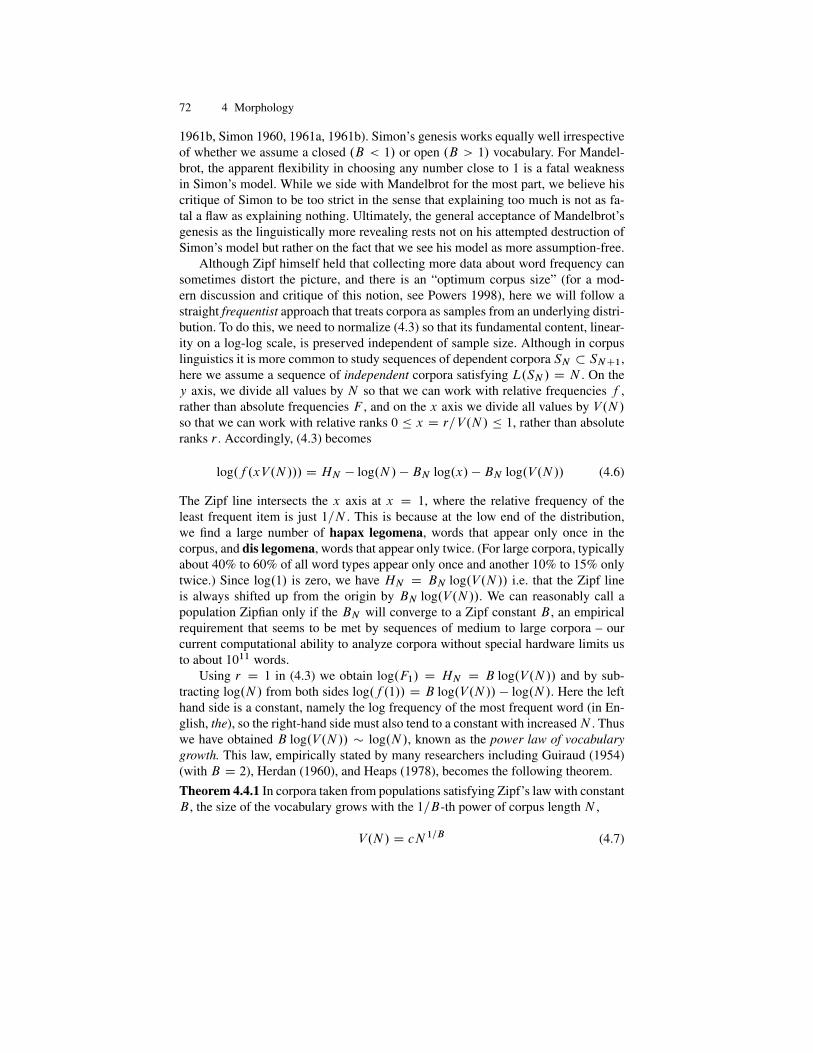
72 4 Morphology

1961b, Simon 1960, 1961a, 1961b). Simon’s genesis works equally well irrespectiveof whether we assume a closed .B < 1/ or open .B > 1/ vocabulary. For Mandel-brot, the apparent flexibility in choosing any number close to 1 is a fatal weaknessin Simon’s model. While we side with Mandelbrot for the most part, we believe hiscritique of Simon to be too strict in the sense that explaining too much is not as fa-tal a flaw as explaining nothing. Ultimately, the general acceptance of Mandelbrot’sgenesis as the linguistically more revealing rests not on his attempted destruction ofSimon’s model but rather on the fact that we see his model as more assumption-free.

Although Zipf himself held that collecting more data about word frequency cansometimes distort the picture, and there is an “optimum corpus size” (for a mod-ern discussion and critique of this notion, see Powers 1998), here we will follow astraight frequentist approach that treats corpora as samples from an underlying distri-bution. To do this, we need to normalize (4.3) so that its fundamental content, linear-ity on a log-log scale, is preserved independent of sample size. Although in corpuslinguistics it is more common to study sequences of dependent corpora SN � SN C1,here we assume a sequence of independent corpora satisfying L.SN / D N . On they axis, we divide all values by N so that we can work with relative frequencies f ,rather than absolute frequencies F , and on the x axis we divide all values by V.N /so that we can work with relative ranks 0 � x D r=V .N / � 1, rather than absoluteranks r . Accordingly, (4.3) becomes

log.f .xV.N /// D HN � log.N / � BN log.x/ � BN log.V .N // (4.6)

The Zipf line intersects the x axis at x D 1, where the relative frequency of theleast frequent item is just 1=N . This is because at the low end of the distribution,we find a large number of hapax legomena, words that appear only once in thecorpus, and dis legomena, words that appear only twice. (For large corpora, typicallyabout 40% to 60% of all word types appear only once and another 10% to 15% onlytwice.) Since log.1/ is zero, we have HN D BN log.V .N // i.e. that the Zipf lineis always shifted up from the origin by BN log.V .N //. We can reasonably call apopulation Zipfian only if the BN will converge to a Zipf constant B , an empiricalrequirement that seems to be met by sequences of medium to large corpora – ourcurrent computational ability to analyze corpora without special hardware limits usto about 1011 words.

Using r D 1 in (4.3) we obtain log.F1/ D HN D B log.V .N // and by sub-tracting log.N / from both sides log.f .1// D B log.V .N // � log.N /. Here the lefthand side is a constant, namely the log frequency of the most frequent word (in En-glish, the), so the right-hand side must also tend to a constant with increasedN . Thuswe have obtained B log.V .N // � log.N /, known as the power law of vocabularygrowth. This law, empirically stated by many researchers including Guiraud (1954)(with B D 2), Herdan (1960), and Heaps (1978), becomes the following theorem.Theorem 4.4.1 In corpora taken from populations satisfying Zipf’s law with constantB , the size of the vocabulary grows with the 1=B-th power of corpus length N ,

V.N / D cN 1=B (4.7)

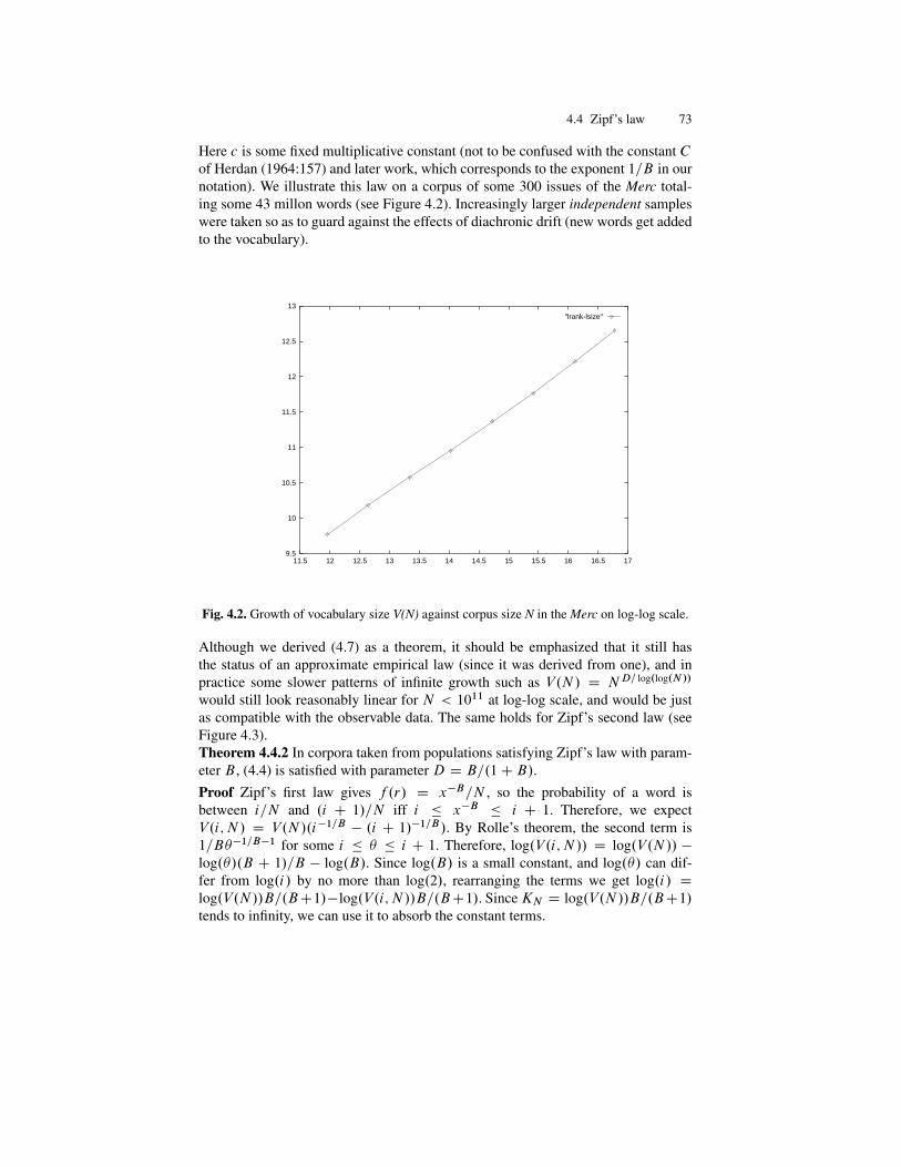
4.4 Zipf’s law 73

Here c is some fixed multiplicative constant (not to be confused with the constant Cof Herdan (1964:157) and later work, which corresponds to the exponent 1=B in ournotation). We illustrate this law on a corpus of some 300 issues of the Merc total-ing some 43 millon words (see Figure 4.2). Increasingly larger independent sampleswere taken so as to guard against the effects of diachronic drift (new words get addedto the vocabulary).

9.5

10

10.5

11

11.5

12

12.5

13

11.5 12 12.5 13 13.5 14 14.5 15 15.5 16 16.5 17

"lrank-lsize"

Fig. 4.2. Growth of vocabulary size V(N) against corpus size N in the Merc on log-log scale.

Although we derived (4.7) as a theorem, it should be emphasized that it still hasthe status of an approximate empirical law (since it was derived from one), and inpractice some slower patterns of infinite growth such as V.N / D ND= log.log.N //

would still look reasonably linear for N < 1011 at log-log scale, and would be justas compatible with the observable data. The same holds for Zipf’s second law (seeFigure 4.3).Theorem 4.4.2 In corpora taken from populations satisfying Zipf’s law with param-eter B , (4.4) is satisfied with parameter D D B=.1C B/.Proof Zipf’s first law gives f .r/ D x�B=N , so the probability of a word isbetween i=N and .i C 1/=N iff i � x�B � i C 1. Therefore, we expectV.i; N / D V.N /.i�1=B � .i C 1/�1=B/. By Rolle’s theorem, the second term is1=B��1=B�1 for some i � � � i C 1. Therefore, log.V .i; N // D log.V .N // �

log.�/.B C 1/=B � log.B/. Since log.B/ is a small constant, and log.�/ can dif-fer from log.i/ by no more than log.2/, rearranging the terms we get log.i/ D

log.V .N //B=.BC1/�log.V .i; N //B=.BC1/. SinceKN D log.V .N //B=.BC1/

tends to infinity, we can use it to absorb the constant terms.

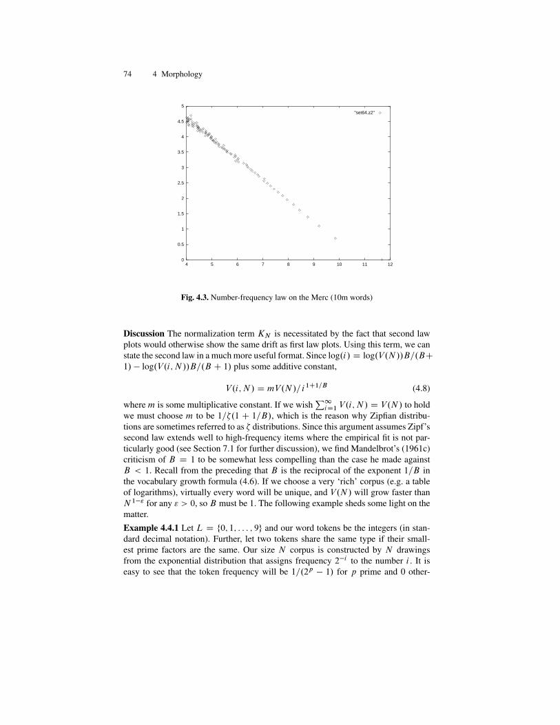
74 4 Morphology

0

0.5

1

1.5

2

2.5

3

3.5

4

4.5

5

4 5 6 7 8 9 10 11 12

"set64.z2"

Fig. 4.3. Number-frequency law on the Merc (10m words)

Discussion The normalization term KN is necessitated by the fact that second lawplots would otherwise show the same drift as first law plots. Using this term, we canstate the second law in a much more useful format. Since log.i/ D log.V .N //B=.BC

1/ � log.V .i; N //B=.B C 1/ plus some additive constant,

V.i; N / D mV.N/=i1C1=B (4.8)

where m is some multiplicative constant. If we wishP1

iD1 V.i; N / D V.N / to holdwe must choose m to be 1=�.1 C 1=B/, which is the reason why Zipfian distribu-tions are sometimes referred to as � distributions. Since this argument assumes Zipf’ssecond law extends well to high-frequency items where the empirical fit is not par-ticularly good (see Section 7.1 for further discussion), we find Mandelbrot’s (1961c)criticism of B D 1 to be somewhat less compelling than the case he made againstB < 1. Recall from the preceding that B is the reciprocal of the exponent 1=B inthe vocabulary growth formula (4.6). If we choose a very ‘rich’ corpus (e.g. a tableof logarithms), virtually every word will be unique, and V.N / will grow faster thanN 1�" for any " > 0, so B must be 1. The following example sheds some light on thematter.Example 4.4.1 Let L D f0; 1; : : : ; 9g and our word tokens be the integers (in stan-dard decimal notation). Further, let two tokens share the same type if their small-est prime factors are the same. Our size N corpus is constructed by N drawingsfrom the exponential distribution that assigns frequency 2�i to the number i . It iseasy to see that the token frequency will be 1=.2p � 1/ for p prime and 0 other-

4.5 Further reading 75

wise. Therefore, our corpora will not satisfy Zipf’s law, since the rank of the i thprime is i but from the prime number theorem pi � i log.i/ and thus its log fre-quency � �i log.i/ log.2/. However, the corpora will satisfy Zipf’s second lawsince, again from the prime number theorem, V.i; N / D N=i2.log.N /� log.i// andthus log.V .N //=2 � log.V .i; N //=2 D log.N /=2 � log.log.N //=2 � log.N /=2C

log.i/C log.log.N / � log.i//=2, which is indeed log.i/ within 1= log.N /.Discussion. Example 4.4.1 shows that Theorem 4.4.2 cannot be reversed withoutadditional conditions (such as B > 1). A purist might object that the definition oftoken/type relation used in this example is weird. However, it is just an artifact of theArabic system of numerals that the smallest prime in a number is not evident. If weused the canonical form of numbers, everything after the first prime could simply bediscarded as mere punctuation.Zipf’s laws, including the power law of vocabulary growth, are near-truths in threedifferent senses. First, the domain of the regularity needs to be circumscribed: it isclear that the empirical fit is not nearly as good at the high end as for lower frequen-cies. Second, these laws are only true in the asymptotic sense: the larger the samplethe better the fit. Finally, these laws are true only as first-order approximations. Ingeneral it makes perfect sense to use not only linear, but also quadratic and higher-order terms to approximate the function of interest. On a log-log scale, however, itis not evident that the next term should come from this kind of approach; there aremany other series that would work equally well.Corollary 4.4.1 Vocabulary is infinite. Since there is no theoretical limit on the sizeof the corpus we can collect, andN 1=B tends to infinity withN , it is a trivial corollaryof the Zipf/Herdan laws that there is no theoretical limit to vocabulary size.

4.5 Further reading

Morphology is historically the oldest layer of linguistics: most of the early work onSanskrit (Pan. ini, circa 520–460 BCE), Greek (Dionysius Thrax, circa 166–90 BCE),and Latin (Stilo, circa 152–74 BCE, Varro, 116–27 BCE) concerns morphologicalquestions. For a clear exposition of the structuralist methods, see Nida (1949). Theidea that paradigms can freely repeat the same form has been raised to a methodolog-ical axiom, known as the Principle of the maximally differentiated paradigm, by oneof the founding fathers of structuralism, Hjelmslev (1961) [1943]. It is not alwaystrivial to distinguish purely phonological from purely morphological concerns, andreaders interested in morphology alone should still consult Anderson (1985). Themost encyclopedic contemporary source is Spencer and Zwicky (1998). The use of(sound, diacritic, meaning) triples is discussed e.g. in Mel’cuk (1993–2000) – Kracht(2003) speaks of exponent rather than sound and category rather than diacritic whenelucidating the same idea of signs as ordered triples.

The prosodic hierarchy is discussed in detail in Hammond (1995); the approachwe follow here is that of Clements and Keyser (1983). How the abstract picture ofsegmental duration assumed in this theory is reconciled with the actual length varia-tion observed in speech is discussed in Kornai (1995 Ch. 3). The sonority hierarchy

76 4 Morphology

originates with Jespersen (1897); for a detailed application to Tashlhiyt Berber [SHI],see Dell and Elmedlaoui (1985, 1988). Moras constitute a still unresolved area; seee.g. Broselow (1995) and Hayes (1995). For the relationship of typology and di-achrony see Aristar (1999). The modern theory of Arabic roots starts with McCarthy(1979); see also Heath (1987). For clitics, see Zwicky (1985), and for bound words,see Nevis (1988).

For the purely phonological part of Pan. ini’s system, see Buiskool (1939). Levelordering in standard phonology is motivated in Kiparsky (1982); for OT-internal ar-guments, see Rubach (1977, 2000); for a synthesis of OT and LPM, see Kiparsky(2006). Opacity was introduced in Kiparsky (1968), for a syntesis of level orderingand OT, see Kiparsky (2006). For an influential modern treatment of blocking, seeAronoff (1976), and for a more detailed discussion of blocking in Pan. ini’s system,see Kiparsky (2002). Note that blocking is not necessarily absolute since doubletslike bicycler/bicyclist can coexist, but (according to Kroch 1994) these are “alwaysreflections of unstable competition between mutually exclusive grammatical options.Even a cursory review of the literature reveals that morphological doublets occurquite frequently, but also that they are diachronically unstable”.

Methods based on character and word frequency counts go back to the MiddleAges: in the 1640s, a Swedish sect was deemed heretical (relative to Lutheran ortho-doxy) on the basis of a larger than expected frequency of forms such as Christ bleed-ing, Christ suffering, Christ crucified found in its Sion Psalmbook. The same powerlaw distribution as Zipf’s law has been observed in patterns of income by Pareto(1897), and there is again a large body of empirical literature supporting Zipf’s law,known in economics as Pareto’s law. Champernowne (originally in 1936, but notfully published until 1973) offered a model where the uneven distribution emergesfrom a stochastic process (Champernowne 1952, 1953, 1973; see also Cox and Miller1965) with a barrier corresponding to minimum wealth. The modern genesis is dueto Mandelbrot (1952) and Miller (1957), though Li (1992) is often cited in this re-gard. Mitzenmacher (2004) is a good survey. The fundamental observation behindHerdan’s law is due to Herdan (1960), though Heaps (1978) is often credited. Theo-rem 4.4.1 is from Kornai (1999a); for a more recent discussion, see van Leijenhorstand van der Weide (2005).

Corpus size has grown dramatically in the past half-century. In the 1960s and1970s the major corpora such as the Brown Corpus, the London-Lund Corpus, or theLancaster-Oslo-Bergen (LOB) Corpus had N D 106 or less. By the 1980s corporawith N D 107–108 were widely disseminated by the Linguistic Data Consortium,and by the 1990s billion-word (109) probabilistic language models were commonlyused; e.g. in speech recognition. Today, monolingual segments of large search enginecaches provide access to corpora such as the Google 5-gram corpus with N > 1012

– inspecting the tail end of such caches makes it clear that infinite vocabulary growthis fueled by compounding and incorporation, as well as certain kinds of affixation(see Kornai 2002 for further discussion).

5

Syntax

The theory of syntax addresses three strongly interconnected ranges of facts. The firstof these is the combinatorical possibilities of words. It is very clear that The boysate is a sentence of ordinary English, while four other permutations of these threeelements, *The ate boys, *Ate boys the, *Boys the ate, and *Boys ate the, are outsidethe bounds of ordinary English. The remaining one, ?Ate the boys, is harder to passjudgment on, but it seems clear that its stylistic value is very different from that of thefirst sentence. Similarly, speakers of English will strongly agree that The boys eat andThe boy eats are ordinary sentences of the language, while *The boy eat and *The boyates are not, a highly generalizable observation that justifies the statement, familiarto all from school grammar, that predicates agree with their subjects in person andnumber.

In most, though not necessarily all, cases it is relatively easy to construct pairsof sentences, one grammatical and the other not, that bring into sharp relief how aparticular rule or constraint operates or fails to operate. There are areas of grammarsuch as ‘weak crossover’ or ‘heavy NP shift’ which are weak in the sense that thecontrast is less visible and obvious than in the examples above, but even if we raisethe bar very high, there are plenty of significant contrasts left for a theory of syntaxto account for. On the whole, the development of syntax is not crucially impactedby the weaker examples, especially as there are generally other languages wherephenomena marginal in one language, such as resumptive pronouns in English, canbe observed in unequivocal examples, and often in far richer detail.

The second range of facts concerns the internal structure of sentences. Generallythere is a verb, which takes a subject, and often an object, sometimes a second (indi-rect) object, and there can be other dependents, modifiers, and so on. Here the prob-lem is twofold: first, it is not at all evident what primitive notions one should consider(though the grammatical tradition of millennia offers some rather clear guidelines),and second, even if a set of primitive grammatical notions is agreed upon, it is farfrom clear which word or combination of words fits which notion in any given sen-tence.

The third range of facts concerns the fit, or lack thereof, between what is beingsaid and what is seen in the world. In Chapter 6, we will view sentences as broadly

78 5 Syntax

analogous to formulas and inquire about their interpretation in various model struc-tures. Here we begin with a word of caution: clearly, people are often capable ofassigning meaning to grammatically ill-formed utterances, and conversely, they canhave trouble interpreting perfectly well-formed ones. But even with this caveat, thereis a great deal of correlation between the native speaker’s judgments of grammati-calness and their ability to interpret what is being said, so a program of research thatfocuses on meaning and treats grammaticality as a by-product may still make sense.

In fact, much of modern syntax is an attempt, one way or the other, to do awaywith separate mechanisms in accounting for these three ranges of facts. In Sec-tion 5.1, we will discuss combinatorical approaches that put the emphasis on the waywords combine. Although in formal theories of grammar the focus of research activ-ity historically fell in this category, the presentation here can be kept brief becausemost of this material is now a standard part of the computer science curriculum, andthe reader will find both classical introductions such as Salomaa (1973) and modernmonographic treatments such as Kracht (2003). In Section 5.2, we turn to grammat-ical approaches that put the emphasis on the grammatical primitives; prominent ex-amples are dependency grammar (Tesniere 1959), tagmemics (Brend and Pike 1976),case grammar (Fillmore 1968), and relational grammar (Perlmutter 1983), as well asclassical Pan. inian morphosyntax and its modern variants. These theories, it is fair tosay, have received much less attention in the mathematical literature than their actualimportance in the development of linguistic thought would warrant. In Section 5.3,we discuss semantics-driven theories of syntax, in particular the issues of frame se-mantics and knowledge representation. In Section 5.4, we take up weighted modelsof syntax, which extend the reach of the theory to another range of facts, the weight agiven string of words has. We will present this theory in its full generality, permittingas special cases both standard formal language theory, where the weights 1 and 0 areused to distinguish grammatical from ungrammatical, the extension (Chomsky 1967)where weights between 1 and 0 are used to represent intermediate degrees of gram-maticality, and the probabilistic theory, which plays a central role in the applications.In Section 5.5, we discuss weighted regular languages, giving an asymptotic charac-terization of these over a one-letter alphabet. Evidence of syntactic complexity thatcomes from external sources such as difficulty of parsing or acquisition is discussedin Section 5.6.

5.1 Combinatorical theories

Given some fixed set of vocabulary items †, a central question is to characterizethe subset L � †� that speakers take to be ‘ordinary’ or ‘grammatical’ or ‘well-formed’ (we use these notions interchangeably) by means of a formal system. Onesignificant practical difficulty is that †, as traditionally understood, collects togetherall words from the language, and this is a very large set. For English, we already havej†j � 106 if we restrict ourselves to words attested in print, and potentially infinite,if we permit all well-formed, but not necessarily attested, words. In Section 5.1.1,we discuss how to define classes of words by distributional equivalence and thereby

5.1 Combinatorical theories 79

replace the set † of words by a considerably smaller set C of (strict) categories. InSection 5.1.2, we introduce categorial grammar as a means of characterizing the setof well-formed expressions, and in Section 5.1.3, we turn to constituent structure.

5.1.1 Reducing vocabulary complexity

Since the vocabulary of natural languages is large, potentially infinite (see Corollary4.4.1), grammarians have throughout the ages relied on a system of lexical categoriesor parts of speech to simplify matters. Originally, these were defined by similarity ofmeaning (e.g. adze and ax) or similarity of grammatical function (e.g. both can serveas the subject or object of a verb). Both these methods were deemed inadequate bythe structuralists:

The school grammar tells us, for instance, that a noun is ‘the name of aperson, place, or thing’. This definition presupposes more philosophical andscientific knowledge than the human race can command, and implies, fur-ther, that the form-classes of a language agree with the classifications thatwould be made by a philosopher or scientist. Is fire, for instance, a thing?For over a century, physicists have believed it to be an action or processrather than a thing: under this view, the verb burn is more appropriate thanthe noun fire. Our language supplies the adjective hot, the noun heat, and theverb to heat, for what physicists believe to be a movement of particles in abody. ... Class meanings, like all other meanings, elude the linguist’s powerof definition, and in general do not coincide with the meanings of strictlydefined technical terms. To accept definitions of meaning, which at best aremakeshifts, in place of an identification in formal terms, is to abandon sci-entific discourse. (Bloomfield 1933 Sec. 16.2)

The method preferred by the structuralists, formalized in contemporary terms byMyhill (1957) and Nerode (1958), relies on similarity of combinatorical potential.Given a word w, we call its distribution the set of all pairs of strings ˛; ˇ such that˛wˇ 2 L. Two words u; v have the same distribution iff

˛uˇ 2 L , ˛vˇ 2 L (5.1)

Strict lexical categories are defined as the equivalence classes C of (5.1). In Sec-tion 3.4 we already introduced a variant of this definition with u; v arbitrary strings(multiword sequences), and we note here that for any strings x; x0 from class c1

and y; y0 from class c2, their concatenation xy will belong in the same distribu-tional equivalence class as x0y0. Therefore, concatenation is a well-defined binaryoperation among the equivalence classes, which is obviously associative since con-catenation was associative. This operation turns C into a semigroup and, with theaddition of the empty word that serves as the identity, a monoid over C called thesyntactic semigroup or syntactic monoid associated with L.

The algebraic investigation of syntax is greatly facilitated by the introduction ofthese structures, which remain invariant under trivial changes such as renaming the

80 5 Syntax

lexical categories. Needless to say, algebraic structures bring with themselves thewhole apparatus of universal algebra, in particular homomorphisms, which are de-fined as mappings that preserve the operations (not just the semigroup product, butin monoids also the identity, conceptualized as a nullary operation); substructures,defined as subsets closed under the operations; and direct products, defined com-ponentwise. We shall also avail ourselves of some notions and theorems more spe-cific to the theory of semigroups and (semi)automata, in particular divisors, whichare defined as homomorphic images of subsemigroups/sub(semi)automata (denotedA � B – when A is a divisor of B , we also say B is a cover of A), cascade prod-ucts, and the powerful Krohn-Rhodes theory. But before we turn to the general casein Section 5.6, here we concentrate on the special case where u; v are words, hereconstrued as atomic symbols of the alphabet rather than as having (phonological ormorphological) internal structure.

By lexical categorization (category assignment) we mean the coarsest one toone (one to many) mapping f W † ! C that respects distributional equivalence. Thesystem of strict categories C employed here is slightly different from the traditionallinguistic notion of lexical categories, in that we do not permit words to have multiplecategories. Where linguists would assign a word such as run two categories, Noun (asin This was a successful run) and Verb (as in Run along!), f maps run to the uniquecategory NounVerb. Also, the finer distinctions relegated in linguistics to the level ofsubcategories, in particular differences among the range of optional and obligatorycomplements, are here seen as affecting the category. Verbs with a single obligatoryargument slot are called intransitive, those with two are called transitive, and thosewith three are called ditransitive. As far as (5.1) is concerned, these are clearlydistinct: compare She ate something (transitive verb) to *She hiccuped something(intransitive verb used in a transitive context). Finally, changes in inflection, viewedby linguists as leaving the category unchanged, have the effect of changing the strictcategories defined by (1): for example, f(eat) ¤ f(eats) because e.g. John eat 62 L

while John eats 2 L.Altogether, the system C of strict categories used here is obtained from the tra-

ditionally defined set of lexical categories or parts of speech (POS) by (i) makinginflection part of the category, (ii) elevating subcategorial distinctions to full cate-gorial status, and (iii) taking the Boolean atoms of the resulting system. Linguisticsgenerally uses a set of only a dozen or so basic lexical categories, presumed to becommon to all languages: the major classes are Noun, Verb, Adjective, Adverb, andperhaps Preposition (or Postposition, depending on language) – given the promi-nence assigned to these in school grammars, these will all be familiar to the reader.There is less agreement concerning minor categories such as Determiner, Pronoun,Quantifier, etc., and many grammarians permit syncategorematic elements that areexempted from the domain of f . By extending the discussion to inflectional distinc-tions, we blow up this basic set to a few hundred or a few thousand, depending onthe complexity of the inflectional morphology of the language in question (Spencerand Zwicky 1998). While in principle the move to Boolean atoms could blow this upexponentially, in practice only very few combinations are actually attested, so thisstep is far less important than the (additive) effect of using strict subcategories.

5.1 Combinatorical theories 81

For English, well-developed sets of categories (usually called tags or POS tagsin corpus linguistics) include the Brown Corpus tagset comprising 226 categories(Greene and Rubin 1971), the LOB Corpus tagset comprising 153 categories (Jo-hansson et al. 1986), and the CLAWS2 and C6 tagsets with over 160 categories(Leech et al. 1994). These numbers are slightly extended by adding subcategorydistinctions within nouns (such as count noun vs. mass noun, simple vs. relational,etc.), adjectives (attributive vs. predicative), and adverbs (manner, time, place, cause,etc.). A far more significant extension comes from adding subcategory distinctionsfor verbs. For example, Levin (1993) distinguished 945 subcategories for Englishverbs, with no two of these having exactly the same distribution. The differences areoften expressed in terms of selectional restrictions. For example murder and kill dif-fer in the requirement imposed on the subject: the former requires a human (compareThe assassin murdered him to *The accident murdered him), while the latter imposesno such restriction (The assassin/accident killed him).

But when all is said and done, the move from the specific lexical items in † tothe strict categories in C brings a great deal of simplification, especially as it col-lapses some very large (potentially infinite) sets such as that of numbers or personalnames. Altogether, the method brings down the size of the alphabet to that of anabridged dictionary, perhaps 103–104 strict categories, sometimes called pretermi-nals in recognition of the fact that they do not correspond well to either the terminalsor the nonterminals in string-rewriting systems. In this regard, we will follow thepractice of contemporary linguistics rather than that of early formal language the-ory and think of terminals as either words or (strict) categories, whichever is moreconvenient.

5.1.2 Categorial grammar

Once we collapsed words with the exact same distribution, the next task is to endowthe set of (pre)terminals with some kind of grammatical structure that will regu-late their combinatorical potential. One particularly attractive method would be toassign each (pre)terminal p 2 C a word s.p/ from a free group G with genera-tors g0; g1; : : : ; gk and define a string of preterminals pi1pi2 :::pir to belong in Liff s.pi1/s.pi2/:::s.pir /, as a group-theoretical product, is equal to a distinguishedgenerator g0 (cf. Example 2.2.2). For reasons that will become clear from the fol-lowing discussion, this method is more attractive in the Abelian than in the general(noncommutative) case, and the latter will require conventions that go beyond whatis familiar from group theory.Example 5.1.1 Arithmetical expressions. Let us collect arithmetic expressions thatcontain both variables and numbers in the formal languageA. For example .1:3�x/�

.1:33C x/ 2 A, but 9/.x 62 A. The major categories, with infinitely many elements,will be Var and Num, and there will be smaller categories Bin for binary operatorsC;�; W;� and Uni for the unary operator �. In addition, we need one-member cat-egories OpenPar and ClosePar. (To eliminate the multiple category assignment ofminus, instead of Bin and Uni we could use StrictBin for C; W;� and BinUni for �,but this would only complicate matters here.)

82 5 Syntax

Since Num and Var give well-formed expressions as they are, we take s(Num) =s(Var) = g0. Members of StrictBin take well-formed expressions both on the left andthe right, so we take s(StrictBin) = g�1

0 – this will work out nicely since g0 �g�10 �g0 D

g0. (Notice that the system slightly overgenerates, permitting the operator to come inPolish or reverse Polish order as well – we will return to this matter later.) The caseof the minus sign is more complicated: when it is a binary operator, it is behavingthe same way as the other operators and thus should get the signature s(�)=g�1

0 , butwhen it is a unary operator it can be prefixed to well-formed expressions and yields awell-formed expression, making it s(�) = IL (left unit). Finally, OpenPar creates anexpression that turns well-formed expressions into ill-formed expressions requiringa ClosePar. To handle this requires a second generator g1, and we take s(OpenPar) =g1g

�10 and s(ClosePar) = g�1

1 g0.Discussion. This toy example already displays many of the peculiarities of categorialgrammar writing. First, whenever a preterminal w belongs to multiple categories,we need to assign it multiple values s(w). In the language of arithmetic, this is arare exception, but in natural language the situation is encountered quite frequently.The categorial signature assignment s thus has to be taken as a one-to-many relationrather than a function, and the key definition of grammaticality has to be modifiedso that as long as there is at least one permitted assignment that reduces to g0, thestring is taken to be grammatical. In a string of r words that are all d -way ambiguousas far as their categorial assignment is concerned, we therefore need to examine d r

products to see if any of them reduce to g0.The main difficulty concerns the left unit. In a group, left units are indistinguish-

able from right units, and the unit will commute with every element even if the groupitself is not commutative. However, in syntax, elements that preserve grammaticalitycan still have order restrictions: consider, for example, the discourse particle well.Ordinarily, if ˛ is a sentence of English, so is Well, ˛, but the string ˛, well will notbe grammatical. To address this issue, categorial grammars formally distinguish twokinds of cancellation, left and right. While in arithmetic 3 � .5=3/ is indistinguish-able from .5=3/ � 3, in categorial grammar we will make the distinction betweenA=B , a syntactic unit that requires a following B to make it A, and BnA, a syntacticunit that requires a preceding B to make it A. If the category of a full sentence isT , the category of well is T=T , meaning that it requires something of category Tfollowing it to yield T . This is in sharp contrast with group theory, where gig

�1i and

g�1i gi would cancel equally (see Section 6.3.2 for further details). By a cancellation

structure we shall mean the minimal set of formal expressions generated from afinite set of basic categories P and closed under the operations .pnq/ and .p=q/.

Once cancellation order is controlled, we are in a good position to capture syn-tactic conventions about arithmetic operators. In standard notation, strictly binaryoperators, such as +, take one argument on the left and one on the right, so theirtype is .gng/=g. In reverse Polish notation, their type is gn.gng/, and in Polish no-tation .g=g/=g. Left units, such as the unary minus operator, can no longer attachanywhere, so expressions like .23:54�/ are now ruled out as long as the type of theunary minus is g=g, demanding a well-formed expression to its right. But the syntaxof natural language still presents some difficulties, even with unary operators like

5.1 Combinatorical theories 83

well. Sentences like Well, well, ..., well, John went home look increasingly strange asthe number of wells increases. This effect has no counterpart in (directional) multipli-cation: if IL is a left unit, multiplying by it many times will not change the outcomein any way. We return to this matter in Section 5.4, where we discuss valuationse.g. in terms of degree of grammaticalness, but here we ignore this complication andsummarize the preceding discussion in two definitions.

A unidirectional categorial grammar is given by a set of preterminals P anda mapping s:P ! 2G , where G is a free Abelian group with a distinguished gener-ator g. We say that the string p1p2 : : : pn is accepted by the grammar iff there areelements of G a1; a2; : : : an such that ai 2 s.pi / and a1a2 : : : an D g.

A bidirectional categorial grammar or just categorial grammar is given by aset of preterminals P and a mapping s:P ! 2G , where G is a cancellation structurewith a distinguished generator g. We say that the string p1p2 : : : pn is accepted bythe grammar iff there are elements of G a1; a2; : : : an such that ai 2 s.pi / andthere is a bracketing of a1a2 : : : an that cancels to g by a series of left- and right-cancellations sanctioned by the rules q.qnp/ D .p=q/q D p.

Categorial grammar (CG) offers an extremely flexible and intuitive method forsorting out complex syntactic situations: schoolchildren spend years mastering thecomplexities that we can now succinctly capture in a handful of categorial signatureassignments. What is particularly attractive about the system is that the syntax ties tothe semantics in exactly the desired manner: the order of cancellations correspondsexactly to the order of evaluation. Take for example 3=2=2. The categorial signaturesare g; gng=g; g; gng=g; g so the product is g, making the expression well-formed.If we begin by evaluating from the left, we first get 3=2 D 1:5, and subsequently1:5=2 D 0:75. If we begin by evaluating from the right, we get 2=2 D 1, andsubsequently 3=1 D 3. Remarkably, the same kind of ambiguity can be observed innatural language. Consider, following Montague (1970a),

Every man loves a woman (5.2)

To keep the notation close to Montague’s original, the distinguished generator g0

will be written T , and the second generator g1 is written E. (Anticipating develop-ments in Section 6.3, T is mnemonic for t ruth value andE for entity.) The categorialsignatures s are given as follows. Common nouns such as man and woman are as-signed the signature T nE. Quantifiers and determiners have signature E=.T nE/,so that noun phrases come out as E=.T nE/ � .T nE/ D E. Finally, transitiveverbs such as loves have signature EnT=E (i.e. they require an E on both sidesto produce the distinguished generator T ). As in the arithmetic example, the products(every)s(man)s(loves)s(a)s(woman)= E=.T nE/ � T nE �EnT=E �E=.T nE/ � T nE

can be computed in two essentially different orders, and these correspond to the tworeadings of (5.2), namely

8xman.x/9ywoman.y/loves.x; y/ (5.3)9ywoman.y/8xman.x/loves.x; y/ (5.4)

84 5 Syntax

It would be trivial to extend this grammar fragment1 to cover proper nouns suchas John by taking s(John) = E, and intransitive verbs such as sleeps by takings(sleeps) = EnT . This would correctly derive sentences such as Every man sleeps orA woman loves John. To add prepositions and prepositional phrases requires anothergenerator P . By assigning prepositions such as to the signature P=E and to ditran-sitives such as gives the signature EnT=E=P , we obtain derivations for sentenceslike John gave a book to every woman. Prefixing adjectives like lazy to commonnouns leaves the category of the construction unchanged: lazy man has essentiallythe same distribution as man. For this reason, we assign adjectives the signature.T nE/=.T nE/. The same method is available for adadjectives like very. Since theseleave the category of the following adjective unchanged, we assign them to the cate-gory ..T nE/=.T nE//=..T nE/=.T nE//.Exercise 5.1. Consider a programming or scripting language with which you arefamiliar, such as Fortran, C, Perl, or Python. Write a categorial grammar that capturesits syntax.

5.1.3 Phrase structure

It is a remarkable fact about natural language that some of the more complex (in lin-guistic terminology, derived) constructions from †� clearly fit in some of the equiv-alence classes of lexical items defined by (5.1). For example, proper nouns such asJohn, and noun phrases such as every man, can be substituted for one another in vir-tually every context such as Bill visited . Comparing John didn’t go home yesterdayevening to ?Every man didn’t go home yesterday evening (to which speakers stronglyprefer No man went home yesterday evening) makes clear that there are exceptions,but the distributional similarity is so strong that our preference is to assume identityand fix the exceptions by a subsequent rule or a more highly ranked constraint.

Not only do proper nouns show near-perfect distributional equivalence with nounphrases, but the same phenomenon, the existence of distributionally equivalent lex-ical entries, can be observed with most, if not all, derived constructions. The phe-nomenon is so pervasive that it has its own name, lexicality. Informally, the principlesays that for any grammatical position or role that can be filled by a phrase, there isa single-word equivalent that can serve in the same position or role. In the specialcase where the equivalence is between a construction and one of its components,this component is called the lexical head of the construction. A good example isadjectival modification: lazy old man is equivalent to its lexical head man. Construc-tions that contain their own lexical heads are called endocentric and the rest arecalled exocentric. Noun phrases formed by determiners or quantifiers are a goodexample of the latter. For example, neither every nor woman shows distributionalequivalence, or even broad distributional similarity, to every woman since the fullconstruction can appear freely in subject or object position, while *Every sleeps,

1 The presentation here is not faithful to the classic Montague (1973) ‘PTQ fragment’ – seeSection 6.2 for details.

5.1 Combinatorical theories 85

*Woman sleeps, *John saw every or *John saw woman are ungrammatical, and con-versely, nouns can undergo adjectival modification while noun phrases cannot (*lazyevery woman). When quantifiers undergo similar modification, as in nearly every,the semantics makes it clear that these do not attach to the whole construction, wehave (nearly every) woman rather than nearly (every woman).

In endocentric constructions, it is nearly always the case that the nonhead con-stituents are entirely optional. This phenomenon, though not quite as general as lex-icality, has its own name: optionality. For constructions composed of two parts, op-tionality follows from the definition: if uv is equivalent to v, this means u was op-tional. For larger constructions, the only exceptions seem to be due to agreementphenomena: for example, Tom, Dick, and Harry is equivalent to Dick and Harry butnot to any smaller substring since the construction (e.g. in subject position) demandsplural agreement. Even exocentric constructions, where there is no clear candidatefor head or for deletable elements, show evidence for not being composed of partsof equal importance, and we commonly find the term head extended to the mostimportant component.

To the extent that there seems to be something of an Artinian condition (no in-finite descending chain) on natural language constructions, we may want to inquirewhether there is a Noetherian condition (no infinite ascending chain) as well. A con-struction whose head is some lexical category c is said to be a projection of c: theidea is that we obtain more and more complex constructions by successively adjoin-ing more and more material to the head lexical entry. Can this process terminate insome sense? Linguistics has traditionally recognized phrases as maximal projections(i.e. as constructions that can no longer be extended in nontrivial ways). The mostimportant example is the noun phrase, which is effectively closed off from furtherdevelopment by a determiner or quantifier. Once this is in place, there is no furtheradjective, numeral, or other modifier that can be added from the left (compare *threethe books, *three every books to the three books, every three books) and only relativeclauses are possible from the right (the three books that I saw yesterday). Once sucha that-clause is in place, again there is no room for different kinds of modifications.Further relative clauses are still possible (the three books that I saw yesterday thatyou bought today), but no other kind of element is. Other notable examples includethe verb phrase (VP), the prepositional phrase (PP), the adjectival phrase (AP), andthe adverbial phrase (AdvP) – since this covers all major categories, it is commonlyassumed that every construction is part of a maximal (phrasal) construction that canbe further extended only by the trivial means of coordination.

Another observation connects nonheads (also called dependents) to phrases: inmost constructions, dependents are freely substitutable for their maximal projections.Thus, where a construction has a dependent adjective, such as traditional in the tra-ditional dish, it can also have a full adjectival phrase, as in the exceedingly traditionaldish. The phenomenon that dependents are maximal projections is common enoughto have a name of its own: maximality.

There are two formally rather different systems of syntactic description built onthese insights. The first, dependency grammar (DG), uses directed graphs wherearcs always run from dependents to heads (in some works, the opposite convention

86 5 Syntax

is used), and the second, X-bar theory, uses string-rewriting techniques. Historically,dependency grammar has not been very concerned with word order, its main focusbeing the relationships that can obtain between a head and its dependents. Stringrewriting, on the other hand, does not really have the apparatus to deal with gram-matical function, valence, case, and similar matters occupying the dependency gram-marian, its primary focus being the hierarchical buildup of sentence structure. In theremainder of this section, we concentrate on X-bar theory, leaving case, agreement,valence, and related issues to Section 5.2.

The key to hierarchical structure is provided by optionality, which enables usto gradually reduce complex constructions to simpler ones. This is the method ofimmediate constituent analysis (ICA), which relies on extending the relation (5.1)from† to†�. Recall Definition 3.4.2: two strings ; ı are distributionally equivalentwhenever

˛ ˇ 2 L , ˛ıˇ 2 L (5.5)

The key insight, due to Chomsky (1956), was to notice that the typical reduction stepin ICA does not require distributional equivalence, just substitutability in positivecontexts:

˛ ˇ 2 L ) ˛ıˇ 2 L (5.6)

To make this concrete, consider the original example from Wells (1947): The king ofEngland opened Parliament. We wish to find how this sentence is built from parts andrecursively how the parts are built from smaller parts, etc. ICA begins with locatingthe structural break between England and opened (rather than, say, between of andEngland) based on the observation that opened Parliament can be substituted by sleptwithout loss of grammaticality and The king of England can be similarly substitutedby the king. It is clear that the substitution works well only in one direction, that ofsimplification. For example, the construction a bed rarely slept in will not toleratesubstitution in the other direction. The famous rule

S ! NP VP (5.7)

captures exactly this step of the ICA. The sentence is analyzed in two constituents, a(subject) NP The king of England and a verb phrase opened Parliament.

In the original notation of Wells (1947), the constituents were described byboundary symbols j; jj; jjj; : : : of ever-increasing strength, so that the sentence wouldcome out The j king jj of j England jjj opened j Parliament, but this has been super-seded by bracketing, which would make the example come out as (((The king) (ofEngland)) (opened Parliament)). In general, to formalize ICA by string rewriting,we need to adjoin new nonterminal symbols to the (pre)terminals found in C or †so as to cover constructions (multiword constituents). Lexicality means that the newsymbols can be patterned after the ones used for categories. Traditionally, the samesymbols, with superscript bars (hence the name X-bar), are reused so that e.g. nounsare N, bare noun phrases are N, and full noun phrases are N. We leave open the issue

5.1 Combinatorical theories 87

of whether there is exactly one bar level between the lexicon and maximal phrasesand use the notation XM to denote a maximal projection of X . (For many minorlexical categories XM D X ; i.e. no complex phrases of that type can be built.) If weattach the nonterminal to the opening parenthesis of each constituent, we speak of la-beled bracketings. Just as scanning codes (see Section 3.4) offer a simple linearizedversion of an association relation, (labeled) bracketings offer a simple linearizationof parse trees, and many questions about tree structures can be recast in terms of thecode strings (Chomsky and Schutzenberger 1963).

Since (5.5) defines an equivalence relation, L itself is the union of some equiva-lence classes. To the extent that sentences are freely substitutable for one another, Lis covered by a single symbol S , the start symbol of string-rewriting systems. Lex-icality in this case is traditionally taken to mean that S is a projection of the mainverb – in more modern accounts it is often some abstract property of the verb, suchas its tense marking, that is taken to be the head of the entire sentence. Either way,rule (5.7) amounts to the statement that the NP on the left (the subject) completes theVP and thus S has one more bar than VP.

In a string-rewriting formalism, maximality means that only rules of the typeXn ! YM

1 : : : YMlXn�1ZM

1 : : : ZMr are possible. Counterexamples are not easy

to find but they exist; consider infinitival clause complements to verbs. Some verbs,such as want, can take both subjectful and subjectless clauses as their complement:compare John wanted Bill to win and John wanted to win. Other verbs, such astry,only take subjectless clauses: John tried to win, *John tried Bill to win. By analogyto tensed sentences, the tenseless Bill to win has one more bar level than to winsince the subject Bill adds one bar. If this is so, the rule expanding try-type VPs hasone fewer bar on the clausal complement than the rule expanding want-type verbs,meaning that maximality is violated in the former. Altogether, maximality remainsone of the fascinating near-truths about syntax, and trying to come to grips with thisand similar counterexamples remains an active area of research.

Given the special role that coordination plays in the system, one technique ofgreat practical significance is extending context-free grammars by permitting rulesof the form A ! r , where r is any regular expression over the alphabet composed ofboth terminals and nonterminals: for any string w that matches r , we say that A canbe rewritten as w. It is easy to see that this extension does not change the generativecapacity of the system (if a language can be described by means of an extendedCFG, it can also be defined by an ordinary CFG), yet the perspicuity of the systemis significantly increased.Exercise 5.2 Prove that extended CFGs only generate CFLs.All in all, (extended) CFGs offer an extremely transparent and flexible method ofsyntactic analysis. Several rather different-looking grammatical traditions are equiv-alent, at least in some formulation, to CFGs: Postal (1964) argued this for tagmemics(Pike 1967), and Bar-Hillel et al (1960) made the argument for categorial grammars.Yet CFGs can be faulted both for over- and undergeneration. On the one hand, CFGscan easily handle the problem of balanced parentheses of arbitrary depth. This isobviously helpful inasmuch as CFGs could not have gained their prominence as the

88 5 Syntax

primary means of syntactic analysis for programming languages without the abilityto correctly handle parenthesized expressions of arbitrary depth, but in the analysisof natural languages, arbitrary depth constructions are rarely encountered, if at all.On the other hand, there is a class of copying phenomena, ranging from cross-serialdependencies (see Section 5.2.2) to constructions such as Freezing cold or no freez-ing cold (we will go barefoot), that is outside the CFL domain, see Manaster-Ramer(1986).

Exploring combinatorical mechanisms that transcend the limitations of CFGshas been, and continues to be, a major avenue of research in mathematical linguis-tics. The general problem of discontinuous constituents, i.e. constituents that areinterrupted by material from other constituents, was noted early by the developers ofICA – for a current summary, see Ojeda (2006b). The fact that cross-serial depen-dencies are problematic for CFGs was noted by Postal (1964), who cited Mohawk[MOH] in this regard – later work concentrated on Germanic languages, in particularDutch and Swiss German. The first formalism to address the issue was tree adjoin-ing grammar (TAG – for a modern summary, see Joshi 2003) and, perhaps evencloser to the original spirit of ICA, head grammars (Pollard 1984). Among catego-rial grammars, combinatory categorial grammar (CCG) provided the same kind ofextension to discontinuities; see Steedman (2001). (Note that where it does not clashwith established mathematical usage, we distinguish combinatorial, ‘pertaining tocombinators’, from combinatorical ‘pertaining to combinatorics’ – CCG uses com-binators.) Readers interested in further details are directed to Chapter 5 of Kracht(2003), which discusses all key developments in this area.

5.2 Grammatical theories

The approaches that put the emphasis on string, tree, or category manipulation arerather new (less than a hundred years old) compared with traditional notions such assubject, object, or case, which grammarians have invoked for millennia in accountingfor syntactic regularities. The primary impulse of the combinatorical theories is todo away with these and similar notions entirely; for example, Chomsky (1981:59)uses (5.7) to define subject as “NP of S” (i.e. as the NP that appears in the rulerewriting S), predicate as “VP of S”, and object as “NP of VP”. Such definitionsimply that there is no explanatory role for these notions in grammar, that they arepurely epiphenomenal, serving at best as convenient abbreviations for constituentsin some frequently seen combinatorical configurations. Yet grammarians not onlypersist in using these notions but in fact the class of theories that rely crucially onthem, what we call ‘grammatical theories’ for lack of a better umbrella term, hasundergone intense development in the past forty years.

The first generative model to give primacy to a grammatical notion of case overthe combinatorical notions of constituency and category was case grammar (Fill-more 1968), and we will cover role and reference grammar (Valin 2005), and rela-tional grammar (Perlmutter 1983), as well as classical Pan. inian morphosyntax andits modern variants (Ostler 1979, Kiparsky 1987, Smith 1996). Over the years, even

5.2 Grammatical theories 89

mainstream combinatorical theory (Chomsky 1981, 1995) came to incorporate mod-ules of case theory and theta theory that employ such grammatical devices.

With the notable exception of lexical functional grammar (LFG; see Bresnan1982) and a variety of unification grammars, which came mathematically fully artic-ulated, the formal theory has not always kept up with the insights gained from thegrammatical work. In Section 5.2.1, we take the first steps toward formalizing someof the key ideas, starting with dependency, agreement, surface case, and government.Deep cases and direct linking are discussed in Section 5.2.2, and grammatical func-tions and indirect linking are discussed in Section 5.3.

5.2.1 Dependency

Classical grammar has imbued our culture to such an extent that many of its techni-cal notions, such as subject, object, or predicate, are applied almost unthinkingly inscientific discourse. So far, we have used these terms without much reflection, essen-tially in the same somewhat vague but nevertheless widely approved sense as theyare used by all people past grammar school. To see what motivates the use of suchdevices, consider first sentence pairs such as

The farmer killed the duckling (5.8)The duckling was killed by the farmer (5.9)

Clearly there is a very close paraphrase relationship between (5.8), known as an ac-tive sentence, and (5.9), known as a passive: it seems impossible to imagine a state ofaffairs in which one is true and the other is false. There is more to active/passive pairsthan semantic relatedness; the constructions themselves show deeper parallelism.Whatever selectional relationship obtains between the active verb and its object iscarried over to the passive verb and its subject, and whatever relationship obtainsbetween the active verb and the subject is replicated between the passive verb andthe agentive by-phrase.

For Chomsky (1957) and much of the subsequent tradition of transformationalgenerative syntax, these observations were taken as indicative of a need to treat (5.8)as basic and (5.9) as derived, obtained from (5.8) by means of a passive transfor-mation that rearranges the constituents of the active construction and supplies therequisite grammatical formatives to yield the passive. Unfortunately, the derivationalanalysis creates as many problems as it solves. In particular, we find actives withno passive counterparts, such as John resembles Bill and *Bill is resembled by John.These require some special mechanism to block the passive transformation. Evenmore problematic are passives with no active counterparts, such as *Everyone saidJohn to be honest/John was said to be honest by everyone, since these call for anobligatory application of the transformation and thus rely on an abstract deep struc-ture. This is extremely challenging from the perspective of language acquisition sincethe learner has to reverse-engineer the path from deep structure to surface based onan opaque surface structure.

90 5 Syntax

That something of a more abstract sort than surface word order or constituencyis required can hardly be doubted, especially if we consider a wider range of alterna-tions. Compare, for example, The butcher cuts the meat/The meat cuts easily to Kellyadores French fabrics/*French fabrics adore easily or Jack sprayed the wall withpaint/Jack sprayed paint on the wall to June covered the baby with a blanket/*Junecovered the blanket over the baby. (The examples are from (Levin 1993), where abroad range of similar alternations are discussed.) Traditional grammatical theories,having been developed on languages that show overt case marking, generally use anabstract version of case as the key mechanism to deal with the subtleties of syntax.

What is case? Structuralist theories of syntax such as Jakobson (1936) took caseto be at the confluence of three major domains: morphology, semantics, and syntax.From the morphological standpoint, surface cases are noun affixes common to allbut the most isolating of languages. The details of case systems vary greatly, fromlanguages such as Hindi that have only two, nominative and oblique (plus a vestigialvocative), to languages such as Hungarian with seventeen and Tsez [DDO] with oversixty morphologically distinct cases. The typical nominative/accusative system willinclude locative cases, accusative, dative, and perhaps some more specialized cases,such as instrumental and genitive (by convention, all nonnominative cases exceptthe vocative are called oblique). Latin, which lacks an instrumental case but has avocative and two locatives, or Russian, are good examples of the typical pattern.

From the semantic standpoint, cases correlate with the role the nouns or NPsmarked by them play in the sentence. In particular, vocative marks the one the sen-tence is addressed to, locatives describe where the action or event described by thesentence takes place, the dative is associated to the recipient or beneficiary, the instru-mental to instruments, and genitive to possession. The correlation between morpho-logical marking and semantic content is far from perfect. For example, in many lan-guages, the same dative morphology will express both recipients and experiencers.Much of traditional syntax is concerned with enumerating the discrepancies, e.g. the‘dative of separation’ that occurs with some verbs instead of the expected ablative,the ‘genitive of material’ which denotes a relationship of ‘being composed of’ as ina bar of gold rather than a relationship of possession, and so forth – we will returnto this matter in Section 5.3.

Finally, from the syntactic side, cases correlate with grammatical function: sub-jects are typically marked with the nominative case, objects with the accusative case,indirect objects with the dative case, and so forth. Again it has been recognized fromthe earliest times that the correlation between grammatical function and case mark-ing is imperfect. On the one hand, we find what appears to be the same functionalrelation expressed by different cases, and on the other, we find that one and the samecase (e.g. the accusative) can serve in different functions. Even so, the syntactic im-pact of case is undeniable. In particular, it is quite clear that in languages with overtcase marking, the noun phrases that carry these marks can generally be permutedmuch more freely than in languages such as English that lack overt case marking.For example, in Latin, we can have anaticulam agricola occisit or any of the otherfive permutations of duckling.ACC farmer.NOM kill.PAST and the meaning of thesentence remains the same as that of (5.8).

5.2 Grammatical theories 91

Here we formalize some essential aspects of grammatical theories, while leavingmany issues open. From a combinatorical perspective, the easiest of these is agree-ment (concord), which obtains between two elements of a construction. The mini-mum requirement for agreement is a set of two words u and v and a paradigmaticdimension D that can take at least two values D1;D2. For example, the words canbe the subject and the predicate, and the dimension can be number, taking the val-ues singular and plural. With the standard glossing notation (see Section 2.3), whereforms are given as x:D with x being a stem and D some paradigmatic value, wehave the following definition.Definition 5.2.1 If for all values Di the strings ˛u:Diˇv:Di 2 L while for alli ¤ j we have ˛u:Diˇv:Dj 62 L, we say that u and v agree in D.In a string-rewriting formalism, agreement is handled by means of complex sym-bols: instead of (7) we write S ! NP:DiVP:Di (the . is used here as part of themorphemic gloss rather than as a pure concatenation marker). Since words can agreein more than one dimension (e.g. the subject and the predicate will generally agreeboth in number and in person), a rule schema like this can be thought of as subsum-ing as many rules as there are Di . This brings to light the phenomenon of internalagreement, when a construction as a whole agrees with some part of it; e.g. boys andlazy boys are both plural, and boy and lazy boy are both singular. Since constructionstypically agree with their heads, the head feature convention (HFC; see Gazdar etal. 1985) stipulates that internal agreement between constructions and their heads isautomatic and it is suspension, rather than enforcement, of this rule that requires aspecial rule.

Note that more than two words can participate in agreement. For example, inGeorgian, the predicate agrees not just with the subject but with the object (andin certain circumstances the indirect object) as well – for a fuller discussion, seeAnderson (1992 Sec. 6.1). The definition naturally extends to situations where oneof the words carries the feature inherently rather than through explicit morphologicalmarking. For example, in Russian, adjectives agree in gender with the nouns theymodify. The nouns do not exhibit gender variation: they are feminine, masculine, orneuter, and have no means of assuming a different value for gender as they couldfor number. In the typical case of concord it is not clear which of the two Di isthe cause and which is the effect. Traditionally we say that the choice of e.g. first-person subject forces first-person verbal morphology on the predicate, but we couldequally well say that the choice of first-person verbal morphology forces the use ofa first-person subject. In the Russian case described above, the direction of the valueassignment is clear: only the adjective has a range of values, so agreement comesfrom the noun imposing its value on the adjective and not the other way around.Such cases are therefore also called government.Definition 5.2.2 If in a construction ˛u:Diˇv:Di 2 L the value Di is an inherentlexical property of u (v), we say that u governs v (v governs u) if ˛u:Diˇv:Dj 62 L

(˛u:Djˇv:Di 62 L) for any j ¤ i:

In dependency grammar, the key diagnostic for assuming a dependency link be-tween two items is agreement. In the special case of government, the direction of

92 5 Syntax

the link is set by convention so that it runs from the dependent to the head (gov-ernor). Since verbs can impose case marking on their complements, verbs are theheads, and not the other way around, a conclusion that in phrase structure grammarwould be reached from a different fact, the optionality of the dependents. The char-acterization of the various dependency relations that can obtain between verbs andtheir dependents is a primary concern of both case grammar, which uses an inven-tory of abstract deep cases to describe them, and relational grammar, which uses thegrammatical functions subject (called ‘1’ in RG), object (‘2’), indirect object (‘3’),as well as more deep case-like functions such as Benefactive and Locative. Otherrelations of note are modification, as obtains between an adjective and a noun or anadverbial and a verb, possession between nouns and nouns, and coreference betweenpronouns and nouns.

Once an inventory of relations is fixed, it is natural to formulate dependencygrammar in terms of directed graphs: words or higher constituents are vertices andthe relations are the edges. A closely related formalism is that of tagmemics, whichuses abstract construction types (called tagmemes) that have empty slots that requirefillers. To this simple dependency apparatus, relational grammar adds an orderedset of strata: conceptually each stratum corresponds to a stage in the derivation.Here we go further, permitting edges to run directly between nodes and other edgesas in traditional sentence diagrams (Reed and Kellog 1878, Kolln 1994, Klammerand Schultz 1996). We take the graph visualization as secondary, and the primaryformalism is given as an algebraic system. For reasons of wider applicability (seein particular Section 5.3) rather than defining a single system, we define a metasys-tem MIL that can be instantiated differently depending on the choice of atoms andoperations.

Definition 5.2.3 (i) The atomic elements of MIL form a finite set A.(ii) The primitive operations of MIL are &, =, and perhaps also finitely many bi-nary operations P1; P2; : : : ; Pn. & will also be denoted by P0, and we use H as a(metalanguage) variable ranging over the Pi .i D 0; 1; : : : ; n/.(iii) If p and q are arbitrary elements, Hpq will be an element, and p D q is an(elementary) statement. The only predicate of MIL is ‘=’. x; y; z; : : : will be (meta-language) variables ranging over elements.(iv) The system is defined inductively: the only elements, operations, and statementsof MIL are those resulting from the iterated application of (iii).(v) The axioms of MIL (using prefix notation for operations and infix for equality)are

x D x

Hx&yz D &HxyHxz&xx D x

H&xyz D &HxzHyz&xy D &yx

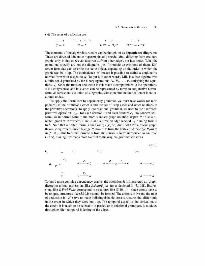
5.2 Grammatical theories 93

(vi) The rules of deduction are

x D y

y D x

x D y; y D z

x D z

x D y

Hxz D Hyz

x D y

Hzx D Hzy

The elements of the algebraic structure can be thought of as dependency diagrams.These are directed labelnode hypergraphs of a special kind, differing from ordinarygraphs only in that edges can also run to/from other edges, not just nodes. What theoperations specify are not the diagrams, just formulaic descriptions of them. Dif-ferent formulas can describe the same object, depending on the order in which thegraph was built up. The equivalence ‘=’ makes it possible to define a conjunctivenormal form with respect to &. To put it in other words, MIL is a free algebra overa finite set A generated by the binary operations P0; P1; : : : ; Pn satisfying the equa-tions (v). Since the rules of deduction in (vi) make = compatible with the operations,= is a congruence, and its classes can be represented by terms in conjunctive normalform. & corresponds to union of subgraphs, with concomitant unification of identicalatomic nodes.

To apply the formalism to dependency grammar, we must take words (or mor-phemes) as the primitive elements and the set of deep cases and other relations asthe primitive operations. To apply it to relational grammar, we need to use a differentprimitive operation Pi;cj

for each relation i and each stratum cj . To connect MILformulas in normal form to the more standard graph notation, depict Piab as a di-rected graph with vertices a and b and a directed edge labeled Pi running from a

to b. Note that a nested formula such as Pia.Pj bc/ does not have a trivial graph-theoretic equivalent since the edgePi now runs from the vertex a to the edgePjab asin (5.10.i). This frees the formalism from the spurious nodes introduced in Gaifman(1965), making it perhaps more faithful to the original grammatical ideas.

(5.10)

(i) b

Pj

��

aPi

//

c

(ii)

aPi // b

cPj // d

(iii)

a bPioo Pj // c

(iv)

a // b

a // d

To build more complex dependency graphs, the operation & is interpreted as (graph-theoretic) union: expressions like &PiabPj cd are as depicted in (5.10.ii). Expres-sions like &PiabPjac correspond to structures like (5.10.iii) – since atoms have tobe unique, structures like (5.10.iv) cannot be formed. The axioms in (v) and the rulesof deduction in (vi) serve to make indistinguishable those structures that differ onlyin the order in which they were built up. The temporal aspect of the derivation, tothe extent it is taken to be relevant (in particular in relational grammar), is modeledthrough explicit temporal indexing of the edges.

94 5 Syntax

An intuitively very appealing way of formulating dependency theories is to in-voke a notion of valences in analogy with chemical valences. Under this conception,grammatical constructions are viewed as molecules composed of atoms (words ormorphemes) that each have a definite number of slots that can be filled by otheratoms or molecules. One key issue is the strength of such valences. Consider forexample

[John]1 rented [the room]2 [from a slumlord]3 [for a barbershop]4

[for the first three months]5 [for fifteen hundred dollars]6 (5.11)

There are a total of six complements here, and most of them are optional: leavingtheir slots unfilled leaves a less informative but still evidently grammatical sentencesuch as John rented. In English at least, the subject (complement 1) is obligatory(*rented a room), and we find many verbs such as admit or transcend that posi-tively require an object (complement 2) as well: consider *John admits or *Johntranscended. Ditransitive verbs require an indirect object (complement 3) as well;compare *John gave, *John gave Bill, and *John gave a last chance to John gaveBill a last chance. These constructions are perhaps analogous to radicals such asCH3, which are not found in nature (because they are so highly reactive that the va-lence gets filled almost immediately). One point where the chemical analogy maybreak down is the existence of situations where one slot is filled by more than onefiller. Superficially, this is what appears in (5.11) with complements 4–6, which areall prepositional for-phrases – the notion of deep cases is introduced precisely withthe goal of separating such complements from one another, see Section 5.2.3 for fur-ther details. Pan. ini distinguishes six deep cases: Agent, Goal, Recipient, Instrument,Locative, and Source (see Staal 1967). The exact inventory is still heavily debated.

5.2.2 Linking

In the Western tradition of grammar, action sentences like (5.8 and (5.9) are viewedas prototypical, and for the moment we will stay with them. Such sentences alwayshave a main verb, and here we assume that verbs come with a case frame that spec-ifies (i) the grammatical relation that the verb has to its dependents, (ii) the case orother marking that expresses this relation, (iii) the syntactic category of the comple-ments, (iv) the obligatory or optional nature of the complements, and (v) the sub-categorization restrictions the head places on the complements. The primary goal ofsyntax, at least in regard to the prototypical class of sentences, is to specify how thevarious entities (NPs) named in the sentence are linked in the argument slots.

Well-developed grammatical theories that rely on case frames include classi-cal DG, head-driven phrase-structure grammar (HPSG; see Pollard and Sag 1987),lexical-functional grammar (LFG; see Bresnan et al. 1982), case grammar (Fillmore1968), role and reference grammar (Foley and van Valin 1984, van Valin 2005), re-lational grammar (Perlmutter 1983), as well as classical Pan. inian morphosyntax andits modern variants (Ostler 1979, Kiparsky 1987, Smith 1996). This is not to say

5.2 Grammatical theories 95

that all these theories are identical or even highly similar. All that is claimed here isthat a linking mechanism, expressed one way or another, is an integral part of theirfunctioning. (Note also that many would take exception to calling this structure acase frame, preferring, often for reasons that make a lot of sense internal to one the-oretical position or another, names such as subcategorization frame, lexical form, orthematic grid.)

Consider again the sentences (5.8) and (5.9). In the active case, we simply saythat the transitive frame shared by kill and many transitive verbs requires a subjectand an object NP (or perhaps an agent and a patient NP, depending on whether ourterminology is more grammatically or semantically inspired). As long as we acceptthe notion that in Latin the relationship of subjecthood (or agency) that holds be-tween the farmer and the act of killing is expressed by overt case marking, while inEnglish the same relationship is expressed by word order, the essence of the analysisremains constant across languages. This is very satisfactory, both in terms of sepa-rating meaning from form (e.g. for the purposes of machine translation) and in termsof capturing variation across languages in typological terms.

In the passive, the central part of the construction is the verbal complex waskilled, which also has two slots in its frame, but this time the second one is optional.The first slot is that of the subject (a passive experiencer rather than an active agent)and must be filled by an NP, while the second, that of the agent, can be left open orbe filled by a by-phrase. There is no sense that (5.9) is derived from (5.8); these areindependent constructions related only to the extent that their main verbs are related.Unlike syntax, which is expected to be fairly regular in its operation, the lexicon,being the repository of all that needs to be memorized, is expected to be storing agreat deal of idiosyncratic material, so the appearance of idiom chunks such as wassaid to be that have their own case frames (in this instance, that of a subject NP anda predicative AP, both obligatory) comes as no surprise.

We still want to say that resemble is an exception to the lexical (redundancy) rulethat connects transitive verbs V-ed to their passive form was V-en, and the case framemechanism offers an excellent opportunity to do so. Instead of taking the verb as aregular transitive (which demands an accusative object), we treat the second com-plement as nonaccusative (e.g. goal) and thereby exempt the verb from the passiverule that operates on true transitives. Such an analysis is strongly supported cross-linguistically in that in many other languages with overt case endings, the secondcomplement is indeed not accusative.

If we connect any specific theory of syntax (among the many variants sketched sofar) to a theory of morphological realization rules (see Section 4.2), we obtain some-thing approaching an end-to-end theory of action sentences, starting with their logi-cal form and going ultimately to their phonetic realization. In a somewhat confusingmanner, both the overall directionality from meaning to form and a specific theory ofsyntax within transformational grammar that uses this direction are called generativesemantics. (The reverse direction, progressing from syntactic form to some kind ofmeaning representation, is called interpretative semantics and will be discussed inChapter 6.) Many theories, such as HPSG (Pollard and Sag 1987) or role and refer-

96 5 Syntax

ence grammar (RRG; see van Valin 2005), are purposely kept neutral between thetwo directions.

To get a richer description of syntax, we need to supplement case frames by anumber of other mechanisms, in particular by rules for dealing with free adverbialsand other material outside the case frame. In (5.11), many grammarians would arguethat the goal adverbial complement 4, for a barbershop, is outside the core argu-ment structure of rent: everything can be said to happen with some goal in view sothis is a free adverbial attached to the periphery rather than the core of the structure.Other supplementary mechanisms include language-particular or universal word or-der rules, rules that govern the placement of dependents of nouns (adjectives, pos-sessors, determiners), the placement of their dependents, and so forth.

Even with these additions, the case frame system has a clearly finitistic flavor. Forevery slot, we need to specify (i) the grammatical relation, taken from a small (typi-cally � 6) inventory, (ii) the case or other marking that expresses the relation, againtaken from a small (typically � 20) inventory, (iii) the syntactic category, typicallya maximal major category, again taken from a small (typically � 5) inventory, (iv)whether the complement is obligatory or optional, a binary choice, and (v) subcate-gorization restrictions, generally again only a few dozen, say � 50, choices. Since averb can never have more than five slots, the total number of case frames is limitedto .6 � 20 � 5 � 2 � 50/5, a number that at 7:7 � 1023 is slightly larger than Avogadro’snumber but still finite. The size of this upper bound (which could be improved con-siderably e.g. by noting that only a handful of verbs subcategorize for four or fivecomplements) gives an indication of the phenomenon we noted in Section 5.1.1 thatnominal, adjectival, and other categories have only a few subcategories, while verbshave orders of magnitude more.

One case of particular interest to modern syntax is whether the frame can becomerecursive: what happens when verbs take other verbs as their complement? The mostfrequent cases, auxiliary verbs and modals such as have or can, are relatively easyto handle because they require main verbs (rather than auxiliaries) to complementthem, which blocks off the recursion in short order. There is a less frequently seenclass of verbs (sometimes called control or raising verbs) that take infinitival com-plements such as try and continue that recurse freely: both John tries to continue torun and John continues to try to run are perfectly grammatical (and mean differentthings). Some of these verbs, such as persuade and want, take sentential infinitivalclauses that have subjects (John persuaded/wanted Bill to run), and the others are re-stricted to infinitival VPs (*John tried/continued Bill to run). To resolve the apparentviolation of maximality (see Section 5.1.3), it is tempting to pattern the latter afterthe former, assuming simply that the subjectless cases already have their subject slotfilled by the subject of the matrix verb by some process of sharing arguments (de-pendents). The issue is complicated by the fact that the behavior of such verbs is nothomogeneous in regard to the use of dummy subjects: compare There continues tobe an issue to *There tries to be an issue – we return to the matter in Section 5.2.3.

Clause (v) of the case frame definition expresses the fact that verbs can ‘reachdown’ to the subcategory of their complements (we have seen an example in Sec-tion 5.1, kill vs. murder) and if some verbal complements are themselves endowed

5.2 Grammatical theories 97

with a case frame, as must be the case for infinitival complements, it is a question forrecursive constructions of this sort as to how far the matrix verb can control the com-plement of a complement of a complement. The answer is that such control can goto arbitrary depth, as in Which books did your friends say your parents thought yourneighbor complained were/*was too expensive? This phenomenon, as Gazdar (1981)has shown, is still easily within the reach of CFGs. There are other significant caseswhere this is no longer true, the most important being cross-serial dependencies,which we will illustrate here on Dutch using a set of verbs such as see, make, help,. . . that all can, in addition to the subject NP, take an infinitival sentence complement(Huybregts 1976). To make the word order phenomena clear, we restrict ourselvesto subordinate clauses beginning with dat ’that’ and leave it to the reader to supply amain clause such as It is impossible . The verbs in question can thus participate inconstructions such as

... dat Jan de kinderen zag zwemmen (5.12)that Jan the child.PL see.PAST swim.INF

that Jan saw the children swim

... dat Piet de kinderen hielp zwemmenthat Piet the child.PL help.PAST swim.INF

that Piet helped the children swim

... dat Marie de kinderen liet zwemmenthat Marie the child.PL make.PAST swim.INF

that Marie made the children swim

Once we begin to recursively substitute these constructions in one another, two thingsbecome evident. First, that there is no apparent limit to this process. Second, theinsertion proceeds at two different sites: both subjects and verbs get stacked left toright.

(5.13)... dat Jan Piet de kinderen zag helpen zwemmen

that Jan Piet the child.PL see.PAST help.INF swim.INFthat Jan saw Piet help the children swim

... dat Jan Piet Marie de kinderen zag helpen laten zwemmenthat Jan Piet Marie the child.PL see PAST help.INF make.INF swim.INF

that Jan saw Piet help Marie make the children swim

98 5 Syntax

The case frames of verbs like see contain a subject slot, to be filled by a nominativeNP, and an infinitival complement slot to be filled by an S.INF, which again is subjectto the rule (5.7) that rewrites it as a subject NP and an (infinitival) VP.INF, and thelatter can be filled by an intransitive V.INF. (Mentioning the INF in these rules is re-dundant since the Head feature Convention will enforce the inheritance of INF fromS to VP to V.) In the DG formalism, the innermost arrow runs from the dependent(subject) child.PL to the head swim.INF. This arrow, corresponding to the innermostVP, is a dependent of the matrix verb make, which has another dependent, the subjectMarie, yielding the complete infinitival sentence Marie make the children swim by(7). Progressing inside out, the next matrix verb is help, with subject Piet and com-plement Marie make the children swim, yielding Piet help Marie make the childrenswim, and the process can be iterated further. In a standard CFG, recursive appli-cation of the rule S.INF ! NP V S.INF, terminated by an application of S.INF !

V.INF, would yield the bracketing [NP V [NP V [NP V]]] as in Piet help Marie makechildren swim, which would be entirely satisfactory for English. But Germanic wordorder does not cooperate: we need to supplement the phrase structure rules either bysome verb second (V2) transformation (den Besten 1985), by a wrapping mechanism(Bach 1980, Pollard 1984), or by a separate linear precedence mechanism to whichwe turn now.

Here the fact that DG is generally silent on word order is helpful: all that needsto be said is stating the typologically relevant generalization (namely that Dutch isV2 in subordinate clauses) to get the required word order. One way to formulategeneralizations about word order is to state them as constraints on linear precedence.In the Dutch case at hand, we can simply say NP � V (noun phrases precedeverbs) within structures dominated by an infinitival S . This technique, called imme-diate dominance/linear precedence, or ID/LP for short, is the one used in generalizedphrase structure grammar (GPSG) (Gazdar et al. 1985). Another possible techniqueis based on nearness, a weakening of the relation of immediate adjacency. If no mor-phological marking is available to signal the fact that two words are strongly related,the best stand-in is to insist that they appear next to each other, or at least as close aspossible. English uses this device for two rather different functions. In parataxis, ad-jacency signals coordination, as in Tom Dick and Harry, where logical calculi wouldrequire Tom and Dick and Harry. The other case is signaling subjecthood: the onlystructural position where a subject can appear is the one immediately before the verb.

Modern theories of morphosyntax (Ostler 1979, Kiparsky 1987, Smith 1996),which differ from Pan. ini chiefly in their ambition to also handle analytic languagessuch as English, have enlarged the inventory of linkers from morphological devicessuch as case marking, prepositions, and agreement to include positionally definedrelationships as well. Direct theories of linking offer a straightforward mechanismto capture the basic intuition with which we started, that cases mediate betweensemantic, morphological, and syntactic generalizations. Their central device is thedeep case (karaka), which serves to link complements to the verb both in sentencesand in nominal constructions derived from verbs. The derivation starts by selecting averb with the appropriate tense marking, some nominals with the appropriate numbermarking, and the deep cases – the latter will be realized (abhihita, ‘spoken’) by

5.2 Grammatical theories 99

morphological and structural devices biuniquely but heterogeneously across verbs.We have biuniqueness in any fixed construction since every deep case that appearsthere will be realized by a single linker and every linker realizes some deep case,and we have heterogeneity in that there is no requirement for the realization to beconstant across verbs. For example, the accusative (surface) case can serve to realizeGoal or Patient (but not both in any given sentence or nominalization), and Goal canalso be realized by the instrumental case.

Such theories are ‘direct’ because they proceed from the arguments of the verb,defined semantically, to the linkers, which are visible on the surface, using only oneintermediary, the deep cases. In contrast, indirect theories invoke two sets of in-termediaries, deep cases and grammatical functions (subject, object, etc.), as well.Relational grammar does not use a separate apparatus for these two (grammaticalfunctions and deep cases are intermingled) but does permit derivational strata, whichmake the overall theory indirect. The same is true of case grammar, which in itsoriginal form (Fillmore 1968) was clearly intended as a direct theory but used trans-formations, which brought strata with them. The case frame definition left room forusing both grammatical functions and deep cases, and so far there is little to recom-mend the traditional notion of grammatical function. Yet there are some remarkablephenomena that point at differences not easily explained without reference to sub-jects and objects. Consider first the behavior of reflexives: John shaved himself isobviously grammatical and *Himself shaved John is obviously not, yet in both casesthe Agent and the Patient of the shaving are both John, so the difference in accept-ability can hardly be attributed to a difference in the semantics.

To further complicate matters, there is a third set of primitives, called thematicroles or theta roles, that are regularly invoked in classifying verbal arguments. Theseare intended as fully semantical, expressing generalizations that follow from themeaning of verbs. For example, if V is an action and NP refers to the Agent ofthis action, then NP intends V to happen. Comparing John accidentally killed thepedestrian to *John accidentally murdered the pedestrian shows that under this defi-nition of Agent (the names used for thematic roles largely overlap the names used fordeep cases), kill does not require an Agent but murder does. The theories of linkingdiscussed so far distinguish between deep and surface cases and keep both of thesedistinct from both grammatical functions (subject, object, indirect object) and the-matic roles to the extent they admit them. Direct theories that refer to thematic rolesuse them purely as abbreviatory devices to distinguish different classes of verbs withdifferent lexical entailments, while indirect theories, to which we now turn, permitcombinatorical statements that refer to more than one set of primitives.

5.2.3 Valency

In Section 5.1 we already considered the informal notion of valency as a means ofstating grammatical regularities. Here we consider a more formal, and in key respectsmore general, mechanism for syntactic computations, the use of algebraic structuresas a means of regulating the computation. We illustrate the way these formal systems

100 5 Syntax

are intended to be used by well-known linguistic phenomena, such as the possessor-possessed relationship, but we do not intend these illustrations to be exemplary inthe linguistic sense. In many cases, different analyses of the same phenomenon arealso available, often within the confines of the same formal systems.

In many languages, such as Latin or German, the genitive case is affixed to a nounto indicate that it is the possessor of another noun (or NP) within the same sentence.The relationship of possession is to be construed as a rather loose one, ranging from‘being a physical part of’, as in John’s hand; to ‘ownership’, as in John’s book; to‘being closely associated to’, as in John’s boss; and to ‘being loosely associatedto’, as in John’s cop, who can be the cop that always tickets John at a particularintersection, the cop that John always talks about, the cop John always calls when afight breaks out in the bar, and so on.

Many linguists, starting with Pan. ini, would argue that the genitive is not evena case, given that it expresses a relation between two nouns rather than a nounand verb. It is also true that the same possessor-possessed relation is expressed inmany languages by suffixation on the head of the construction, the possessed ele-ment, rather than on the modifier (the possessor). For our purposes, the main fact ofnote is that the possessor can show agreement with the possessed in head-markinglanguages. For example, Hungarian az en konyvem, a te konyved, az o konyve ‘mybook, your book, his book’. By Definition 5.2.1, this means that in the pure casewe have some forms u:Di and v:Di that cooccur in some context ˛ ˇ , while fori ¤ j; ˛u:Diˇv:Dj 62 L. (Not every case is pure since often the paradigmaticdistinction is not entirely visible on the form, such as English you, which can besecond-person singular or plural, or Hungarian az o, which in the possessive con-struction can be third-person singular or plural possessor alike. As there are manylanguages where all paradigmatic forms are distinct, we can safely ignore this com-plication here.)

Since there are only a finite number of cases to consider, almost any method, in-cluding tabulation (listing), would suffice to handle agreement phenomena like this.For example, if the paradigm has four slots and we denote u:Di .v:Di / by a,b,c,d(resp. a0; b0; c0; d 0), the four forms ˛aˇa0 ; ˛bˇb0 ; ˛cˇc0 ; ˛dˇd 0 are admissi-ble, while ˛aˇb0 and the other eleven nonagreeing forms are not. Yet linguisticsrejects this method since the intrinsic complexity of such a list would be the ex-act same as that of listing the cyclic permutation ˛aˇb0 ; ˛bˇc0 ; ˛cˇd 0 , ˛dˇa0 ,and the latter is clearly unattested among natural languages. The preferred methodis to formulate a rough rule that generates ˛uˇv and supplement this by a furthercondition stipulating agreement between u and v.

One important method of stipulating such conditions is to map preterminalsonto some algebraic structure that offers some direct means of checking them. Forexample, given a free group F over four generators a, b, c, d and their inversesa0 D a�1; b0 D b�1; c0 D c�1; d 0 D d�1, if ˛; ˇ; and are mapped on the unit eof F and a; : : : ; d; a0; : : : ; d 0 onto themselves, the acceptable forms, the ones withproper agreement, will be exactly the ones whose image is mapped onto e. Whatmakes cancellation in a group such an attractive model of valency is that it is easilytyped. When talking about valence informally, we always mean finding an appro-

5.2 Grammatical theories 101

priate filler for some slot. By assigning each slot an independent group element andeach appropriate filler its inverse, we can guarantee both that slots will require fillingand that different slots receive different fillers.

Given that agreement in natural languages is independent of word order, the factthat in a group we always have aa�1 D a�1a D e is useful, and so is the fact that wecan take the group used for checking agreement to be the direct product of simplercyclic groups used for checking agreement in any particular paradigmatic dimension.But in situations where the filling of valences is order-dependent, using structuresother than groups and using decomposition methods other than direct products maymake more sense. Before turning to these, let us first consider other potential pitfallsof modeling valences with cancellation.

A strong argument against a strict cancellation model of valency may be a casewhere a single slot (negative valence) is filled by more than one filler (positive va-lence), as in coordinated constructions, such as John and Mary won, or conversely,cases where a single filler fills more than one slot. Consider, for example, the ac-cusativus cum infinitivo (ACI) construction in Latin, as in Ad portum se aiebat ire‘He said he (himself) was going to the harbor’. Evidently the reflexive pronoun se‘himself.ACC’ acts both as the subject of say and the subject of go. On the whole,the scope of ACI in Latin is remarkably large: almost every verb that can take anobject can also take an infinitival construction as an object. Unlike in English orDutch, where He wanted/helped/watched the children to swim are possible but *Hesaid/judged/delighted the children to swim are not, in Latin sentences such as Thalesdixit aquam esse initium rerum, Karthaginem delendam esse censeo, and Gaudeo tesalvum advenisse are easily formed. Another potential case of a single filler fillingmultiple slots comes from the class of control verbs discussed in Section 5.2.2: inJohn tried to run, arguably the same filler, John, acts as the subject of try and run atthe same time. Even more interesting are cases of object control such as John askedBill to run, where Bill is both the object of ask and the subject of run – compare Johnpromised Bill to run.

To extend valency to coordination, we need a device that will act as a multiplexerof sorts, taking two syntactic objects with one positive valence each and returninga single compound object with one positive valence. Problems arise only in caseswhere the compound filler can appear in positions that are closed off for elementaryfillers: clearly John and Mary hated each other is grammatical, while neither *Johnhated each other nor *Mary hated each other are, and it is hard to conceive of theformer as being in any sense the coordination of the latter two. Once a multiplexer isavailable, it or its dual could be used for unifying slots as well, and expressing generalstatements like ‘in object control verbs, the object of the matrix verb is shared withthe subject of the embedded verb’ would be easy.

Yet, just as with coordination, there remain some strong doubts whether usingargument sharing as a conceptual model for apparently shared fillers is truly appro-priate. For example, I hate to smoke means that I dislike cigarette smoke, while I hatethat I smoke means that I actually like cigarette smoke (but dislike my own weaknessof not being able to give it up). The standard method of formalizing argument sharingis by means of shared variables: if we treat transitive verbs as two-place predicates,

102 5 Syntax

try(Someone, Something), hate(Someone, Something), and intran-sitives as one-place predicates, run(Someone), or as two-place predicates withimplicit defaults, smoke(Someone,Cigarettes), we can write John tried torun as x=John, try(x,run(x)) and I hate to smoke as x=I, hate(x,smoke(x,Cigarettes)), but this representation is clearly more appropriate forI hate it that I smoke.

How, then, is I hate to smoke to be represented? One possibility is to treat ‘hating-of-smoking’ as a compound verb that has only one valence and relegate the processof forming such verbal complexes to the lexicon, where other valency-changing pro-cesses, such as forming passives or causatives, are also known to operate. In syntax,then, we can retain a pure form of valence theory that assigns a valence of C1 toevery NP, including coordinated forms, and a valence of �n to n-place predicates.However, the situation is further complicated by free adverbials and other adjunctNPs that do not fill any slot associated to the verbal arguments – this is what makestyping the slots and fillers essential.

In the commutative case, we can restate matters using additive rather than mul-tiplicative inverses and direct sums rather than direct products. We will say that apredicate has a valence vector .x1; : : : ; xk/, where the xi are 0 or �1 and the ba-sis dimensions correspond to grammatical functions or deep cases – for the sake ofconcreteness, we will use Agent, Goal, Recipient, Instrument, Locative, and Sourcein this order. The valence vector of rent will thus be .�1;�1; 0;�1;�1;�1/, andfor our example (5.11), John rented the room from a slumlord for a barbershopfor the first three months for fifteen hundred dollars, we have five NPs that can fillthe slots: John as the Agent, with valence vector .1; 0; 0; 0; 0; 0/; the room as theGoal, with valence vector .0; 1; 0; 0; 0; 0/; a slumlord as the Source, with valencevector .0; 0; 0; 0; 0; 1/; the first three months as the Location, with valence vector.0; 0; 0; 0; 1; 0/; and fifteen hundred dollars as the Instrument, with valence vector.0; 0; 0; 1; 0; 0/. The purpose clause, for a barbershop, is floating freely (the Goal isthe immediate result of the renting action in view, namely the room) and thus hasvalence vector .0; 0; 0; 0; 0; 0/. As long as the valence vectors sum to 0, we acceptthe sentence, seemingly irrespective of phrase order; the reason why *John the roomrented is unacceptable is that in English only the NP in the immediate preverbal po-sition can be the Agent and only the NP in immediate postverbal position can bethe Goal. In languages where deep cases are morphologically marked (by surfacecases), the expectation is that the clauses can be freely permuted as long as theirmorphological marking is preserved.

5.3 Semantics-driven theories

In the most extreme form of semantics-driven theories of syntax, the relation thatconnects the form and the meaning of sentences is one of causation: a sentence has agiven form because this is the best way to express some idea or state of affairs. Giventhe bewildering variety of ways different languages can express the same thought,this appears a hopelessly naive approach, yet a great deal of the methods and motiva-

5.3 Semantics-driven theories 103

tion are shared between the semantics-driven and the more ‘pure’ theories of syntaxdiscussed so far. To solve the problem that different languages use different construc-tions to express the same idea, all that is needed is a parametric theory of syntax anda slight relaxation of direct causality. Instead of saying that a sentence has a givenform because this is the best way to express an idea, we now say that it has this formbecause this is the best given the language-specific setting of the parameters.

To give an example, consider transitive sentences of the (5.8) type. Semantics-driven theories maintain that the structure of thought is universal: there is an actof killing, with the farmer as the agent and the duckling as the patient. FollowingGreenberg (1963), we divide languages in six types corresponding into the six pos-sible permutations of Subject, Object, and Verb. English is an SOV language, so thesentence comes out as above. In Japanese, an SOV language, we get Hyakusyoo waahiru o korosita ‘As for farmer, duck killed’, while in Irish, a VSO language, we getMhairiagh an feirmeoir an lacha, and so forth. Given that word order in differentlanguages can take any value (according to Hawkins (1983), 45% of languages areSOV, 42% SVO, 9% VSO, 3% VOS, 0.9% OVS, and 0.1% are OSV), proponentsof the Sapir-Whorf hypothesis must explain why the majority of languages do notfollow the natural order (whichever that may be).

The research program of eliminating nonparametric variation from syntax iscommon to many theories, including some of the most pure combinatorical theo-ries, such as classical transformational grammar and modern minimalist syntax. Thestandard form (see Chomsky and Lasnik 1993) is often called principles and param-eters theory, assuming a common core of grammatical principles that operate in alllanguages, and a finite set of binary parameters that govern them (so that altogetherthere are only finitely many core systems). This is an extremely attractive model, butone that faces many serious technical difficulties that come to light as soon as we at-tempt to flesh out the typological system. First of all, there are many languages thatare split (display a mixture of the pure types). For instance, German, while widelyregarded as an SOV or V2 (verb second) language, displays a pure SVO constructionand has several different word orders both in main and in subordinate clauses. Tradi-tional descriptions of German word order, such as Drach (1937), therefore employ alinear structure composed of separate structural positions or topological fields, a no-tion that has little typological generality. Even if we could separate out the parochialfrom the universal factors in such cases, there is a larger problem: the terms thatwe use in establishing our typology may have no traction over the actual variety oflanguages.

The marked word orders VOS, OVS, and OSV account for less than 5% of theworld’s languages. However, about one language in ten has no identifiable subjectcategory at all according to Schachter’s (1976) criteria: a prime example is Acehnese[ACE] (see Durie 1987). For many languages that fall outside the Greenberg sys-tem entirely, a different typological distinction between ergative and accusative lan-guages is invoked. As the basic pattern is very strange for those whose only exposurehas been to the 90% of languages that are accusative, we give an example here fromWarlpiri [WBP] (Hale 1983). The sentences generally considered simplest are theintransitives. These involve just a single argument:

104 5 Syntax

The baby cried (5.14)NP.NOM V.PAST

and in the familiar accusative languages that have overt case marking, this argument,the subject, appears with the nominative case. Transitives, the next simplest case,require two arguments. We repeat example (5.8) here with the relevant pseudogloss:

The farmer killed the duckling (5.15)NP.NOM V.PAST NP.ACC

That the glosses in (5.14) and (5.15) are not entirely fictitious even for English isclear from the use of oblique pronouns him/her in the object position as opposed tothe nominative he/she in the subject position. The Warlpiri pattern is rather different:

Kurdu ka wangka-mi (5.16)NP.ABS AUX speak.NONPAST

The child is crying

Ngarrka-nguku ka wawirri panti-rni (5.17)man.ERG AUX kangaroo.ABS spear.NONPAST

The man is spearing the kangaroo

What is striking about this pattern (which is the basic pattern of languages calledergative in typology) is that the default case marking (called absolutive and realizedby zero morphology in many ergative languages, just as nominative is realized byzero in many accusative languages) appears with what from the accusative perspec-tive we would consider the object of the transitive construction, and it is the subjectthat receives the overt case marking. As this example shows, it is far from trivialto put to use grammatical primitives such as subject or object even for their statedpurpose of grammatical description – ergative languages group together the subjectsof intransitives with the objects of transitives.Example 5.3.1 The basic accusative pattern. In defining the accusative and ergativepatterns, we put to use the algebraic apparatus we started to develop in Section 5.1.1.For both cases, we will have nominal elements in the category n (John, the baby),purely intransitive verbs (sleeps, walks), purely transitive verbs (loves/kills), andverbs that have both kinds of subcategorization (eats, sees), which we place in cate-gories i , t , and d , respectively. To simplify matters, we shall ignore person/numberagreement but obviously not case marking. For the relevant case suffixes, we will useN (Nominative) A (Accusative), B (aBsolutive), and E (Ergative), and since thesealways attach to nominal elements we will treat them as subcategories of n, writing

5.3 Semantics-driven theories 105

simply A instead of the morphemic gloss n.A. The accusative pattern is given by afinite language X that will have the strings corresponding to intransitive and tran-sitive sentences, with the appropriate case markings Ni, NtA, Nd, NdA and all theirpermutations (free word order).

The syntactic monoid CX has two distinguished elements: the empty string(whose equivalence class we denote by I since it is the multiplicative identity) anda large grab-bag equivalence class U for all strings with more than one verbal ormore than two nominal elements. Members of this class are all cases of unrecover-able ungrammaticality in the sense that no further element can be added to create agrammatical sentence. Other strings, such asNA, are also ungrammatical, but in a re-coverable way: adding d or t to the string will create a grammatical sentence, and infact it simplifies matters to arrange all equivalence classes in layers running from theinnermost .I / to the outermost .U / in accordance with how many further elementsit takes to make them grammatical. In the innermost layer, we find two classes, rep-resented by t and A, respectively (these require two further elements to complete asentence), in the next layer we find five classes, represented by Nt; i; NA;N , andd , respectively (these require only one further element), and in the outermost layerwe find two classes represented byNi andNd , respectively (both require zero addi-tional elements, but they are not in the same class since for one A can still be added).Altogether, the four basic grammatical strings in the accusative pattern (or five, if wedeclare the empty string grammatical) and their permutations yield a total of elevensyntactic congruence classes i.e. a syntactic monoid with eleven elements.Discussion The progression from inner to outer layers is a way of recapitulating theidea of valency discussed in Section 5.2.1, and serves to show an essential propertyof the system, namely that no simple sentence ever has a (semigroup-theoretic) in-verse: once valencies are filled in, there is no return. Complex sentences (with morethan one verb) may still show periodic behavior (by filling in a verbal dependent wemay end up with more open valences than when we started out), but the syntacticsemigroup built on simple sentences will always be aperiodic. Since this result isclearly independent of the simplifying assumption of free word order made above,we state it as a separate postulate.

Postulate 5.3.1 In any natural language, the syntactic monoid associated to the lan-guage of simple sentences is aperiodic.In Chapter 2, we already emphasized the importance of Chomsky’s (1965) observa-tion that natural languages are noncounting in the informal sense that they do notrely on arithmetic notions. Postulate 5.3.1 provides a more formal statement to thesame effect, and in Section 5.5 we shall offer a formal definition of noncounting thatis, perhaps, easier to falsify empirically than Postulate 5.3.1, but as Yli-Jyra (2003)notes, even a large-scale wide-coverage grammar of English (Voutilainen 1994) canbe modified to avoid the Kleene � operator altogether. Note, however, that the state-ment is clearly relevant only for syntax since phonology evidently shows periodicpatterns, e.g. in the placement of stress (typically binary, sometimes ternary), as dis-cussed in Section 4.1. This runs counter to the generally unspoken but neverthelessvery real prejudice of early generative grammar that phonology is easier than syntax.

106 5 Syntax

Returning to the ergative pattern for a moment, the language Y will have Bi, EtB,Bd, EdB, and their permutations. It is a trivial exercise to verify that the monoid CY

is isomorphic to CX . By mapping N to B and A to E, the accusative set of patternsis mapped on the ergative set in a concatenation-preserving manner. However, thisis an isomorphism that fails to preserve meaning: The man is spearing the kangaroowould become The kangaroo is spearing the man, and it is easy to see that in factno meaning-preserving isomorphism exists between the two patterns. We return tothis matter in Chapter 6, where we investigate not just the stringsets but rather morecomplex structures that contain both the words and their meanings.

The study of the ergative pattern makes it abundantly clear that the overall planof using a few examples and counterexamples to help navigate the typological deci-sion tree is very hard to put into practice. Compared with stress typology (see Sec-tion 4.1.4), the situation is rather dismal. The empirical correlates to the primitivenotions are unclear, and the system, however organized, is riddled with split cases.For example Dyirbal [DBL] has an accusative system in the first and second persons,ergative in the third person (Schmidt 1985), and many Indo-Iranian languages areergative in perfect and accusative in imperfect aspects and so on.

This gives rise to the suspicion, shared by many in the field of artificial intelli-gence (AI), that mainstream linguistics goes about the whole matter the wrong way,invoking too many hard to define and hard to apply grammatical intermediaries inwhat should be a straightforward mapping from thought to expression. The goalshould be simply to specify the language of thought and explain syntactic complexi-ties, to the extent we care about them, by means of parochial imperfections in naturallanguages. This line of thought goes back at least to the great rationalist thinkers ofthe 17th century, in particular Descartes, Pascal, and Leibniz. Early AI research suchas Quillian’s (1969) Teachable Language Comprehender and Anderson and Bower’s(1973) Human Associative Memory and the subsequent ACT-R took quite seriouslythe task of accounting for human long-term memory, including performance effectssuch as reaction times.

In modern research, the mental aspects of the language of thought are generallydownplayed, with many researchers being downright hostile to the idea of lookingfor brain activity correlates to formulaic descriptions of thoughts or ideas. Rather,to eliminate any reference to the mental aspects, emphasis is placed on what thethoughts or ideas are about, in particular on real-world objects (entities) and asser-tions about them.

In this view, the task of knowledge representation (KR) begins with hierarchicallyorganizing the entities that are typically expressed by common nouns. The centralorganizational method is Aristotelian, with increasingly special species subsumedunder increasingly general genera. Economy is achieved by a system of default in-heritance whereby lower nodes on the hierarchy inherit the properties of the highernodes unless specified otherwise. Thus, we need not list the property of breathingwith Baby Shamu since she is a killer whale, killer whales are dolphins, dolphins aremammals, mammals are animals, and animals breathe. However, the inference thatfishes breathe has to be blocked by explicitly stating that fishes do not breathe air,that indeed breathing water through gills is part of their definition. (Going further,

5.3 Semantics-driven theories 107

the default fish rule needs to be suspended for lungfish and other fish species that canin fact breathe air.) The creation of systems of logic that can sustain nonmonotonicinferences (overriding default conclusions in special cases) is an important thread inmodern AI and philosophical logic (see Ginsberg 1986a, Antonelli 1999).

Linguists have long used this technique to hierarchically classify lexical entries,in particular verbs. At the top of the hierarchy, we find the telic/atelic distinction thatroughly corresponds to the count/mass distinction among nouns. Telic verb phrasesdenote events that have a definite endpoint, while atelic VPs lack this; compare Johncleaned the dishes for an hour to *John recognized Bill for an hour. Next, atelicevents are divided into states and activities, telic events into achievements and ac-complishments; see Vendler (1967), Dowty (1979), and Verkuyl (1993). The situa-tion is greatly complicated by the existence of other largely orthogonal classificationschemes such as stage-level and individual-level predicates (for a modern summary,see Kratzer 1995) or other semantically motivated groups such as verbs of motionor psych verbs. Levin (1993) offers a rich selection of grouping criteria but refrainsfrom hierarchically organizing the data and thus avoids the need to specify exactlywhat aspects of the competing cross-classification schemes inherit and to what extentthe different flavors can be mixed.

Just as common nouns correspond to entities, adjectives correspond to properties.Unlike entities, which are taken to be an atomic type E, properties are taken asfunctions from entities to truth values T . Under this analysis, the meaning of anadjective a is simply the set of entitiesN such that a.n/ is true, and n enjoys propertya just in case n 2 N . A key aspect of this model is the division of properties thatan entity has into accidental and essential properties. Continuing with the exampleabove, not only do fishes breathe water but this is essential to their being fishes. Thefact that they generally have iridescent scales is accidental: we can imagine fisheswithout this property, and indeed we find many, such as sharks or eels, that have nosuch scales. What is accidental in one kind of entity may be essential in another,and to keep track of which is which Minsky (1975) introduced the notion of frames.These are not to be confused with the case frames introduced in Section 5.2 above –KR frames apply to nouns, case frames to verbs.

For example, the dog frame will contain slots for name and owner, which areessential to the definition of dogs as cultural constructs in modern urban life, eventhough they would not be relevant for a biological definition. That it is indeed thecultural, rather than the biological, definition of dogs that is relevant to concernsof natural language understanding can be seen from the following examples: Roverhas diarrhea. The owner has a hard time complying with cleanup regulations/*Thecoenzyme Q10 overdose is evident. Once Rover has been introduced to the discourse,referring to the owner proceeds smoothly because the former is a definite (singular)entity and as such implies a definite owner. For people outside the medical and vet-erinary professions, the relationship between dogs, diarrhea, and coenzyme Q10 isanything but evident, and introducing coenzyme Q10 overdose with the definite arti-cle the is infelicitous.

For another example, consider the dictionary definition of cup as a usually openbowl-shaped drinking vessel with or without a handle. What does this really mean?

108 5 Syntax

Clearly, every individual object is with or without a handle, and it is just as true ofthe genus fish that it comes with or without a handle as it is of the genus cup. Yetthere is something right about the definition: I found a cup/*fish but the handle wasbroken shows the same effortless move from cup (but not from fish) to handle thatwe had from dog to owner. So the cup frame must contain a slot for handle meaningthat having a handle, or not, is an essential property of cups.

Frames extend more or less naturally to events. To avoid confusion with caseframes, we call the frame representation of event objects scripts, as has been stan-dard in KR since the work of Schank and Abelson (1977). The original intentionwas to use scripts as repositories of commonsense procedural knowledge: what todo in a restaurant, what happens during a marriage ceremony, etc. Scripts have ac-tors fulfilling specific roles, e.g. that of the waiter or the best man, and decomposethe prototypical action in a series of more elementary sub-scripts such as ‘presentingthe menu’ or ‘giving the bride away’. There are some linguistically better motivatedmodels, in particular discourse representation theory, that rely on lexically storedcommonsense knowledge, but their scope is more modest, being concerned primar-ily with the introduction of new entities (the owner, the best man) in the discourse.Also, there are more systematic studies of ritual, in particular in the Indian tradi-tion (Staal 1982,1989), but their cross-fertilization with the Western KR traditionhas been minimal so far.

The AI program, then, offers specific solutions to many issues surrounding therepresentation of nouns, adjectives, and verbs, with both active and stative verbsfreely used as elementary subunits in scripts. In fact, these subunits are not viewedas atomic: conceptual dependency (Schank 1972) is a representational theory that ex-tends ideas familiar from dependency grammar down to the level of mental language.To apply the MIL formalism of Section 5.2 to Conceptual Dependency, we take theprimitive objects to be the atomic symbols PP, PA, and AA (which in CD correspondroughly to nouns, adjectives, and adverbs), ATRANS, PTRANS, MTRANS, GRASP,PROPEL, MOVE, INGEST, EXPEL, ATTEND, SPEAK, MBUILD, and DO (whichcorrespond roughly to verbs), and choose thePi as CAUSE, BI-CAUSE, MOBJECT,INSTRUMENT, ENABLES, RESULTS, INITIATES, and REASON (which corre-spond roughly to cases).Exercise 5.2 Consider all the English example sentences in Chapter 6 and write theequivalent graphs and formulas.This skeletal picture would need to be supplemented by a host of additional axiomsto recapitulate the exact combinatorical possibilities of CD, e.g. the notion that ob-jects need to be AT-LOC before they can PTRANS out of it (Schank 1973). We willnot pursue CD in this detail because the representations preferred in linguistics tendto use a slightly different set of primitives; e.g. for John gave the book to Bill wecould have DO(John,CAUSE(HAVE(Bill,book))) as the underlying semantic struc-ture (Jackendoff 1972). The explicit use of implicit illocutionary primitives such asDO in this example is particularly characteristic of the generative semantics school(Harris 1995).

5.3 Semantics-driven theories 109

An important version of the same broad program has been pursued by Wierzbicka(1972, 1980, 1985, 1992) and the NSM school (Goddard 2002). The set of prim-itives is broader, including pronouns I, YOU, SOMEONE, SOMETHING/ THING;determiners THIS, THE SAME, OTHER; quantifiers ONE, TWO, SOME, ALL,MANY/MUCH; adjectives GOOD, BAD, BIG, SMALL, TRUE; adadjectives VERY,MORE; verbs THINK, KNOW, WANT, FEEL, SEE, DO, HEAR, SAY, HAPPEN,MOVE, TOUCH, LIVE, DIE; adverbials WHERE/PLACE, HERE, ABOVE, BE-LOW, FAR, NEAR, SIDE, INSIDE, TOUCHING, WHEN/ TIME, NOW, BEFORE,AFTER, A LONG TIME, A SHORT TIME, FOR SOME TIME; connectives NOT,MAYBE, CAN, BECAUSE, IF; relations KIND OF, PART OF, THERE IS/EXIST,HAVE, LIKE; and a handful of nouns: BODY, WORDS, MOMENT, PEOPLE (ele-ments in italics were included in the early work, the rest were added since the 1990s).Unlike many of the early AI researchers whose work aimed at immediate algorith-mization, Wierzbicka and the NSM school, with a commendable lack of pretense,eschew formalization and operate entirely with natural language paraphrases such asthe following definition (Wierzbicka 1992:36) of soul:

one of two parts of a personone cannot see itit is part of another worldgood beings are part of that worldthings are not part of that worldbecause of this part a person can be a good person

To recapitulate this analysis in a more formal framework, we would need to intro-duce two worlds, one with visible things and one without, a conceptual model ofpersons with parts in both worlds, goodness and visibility (or the lack thereof) asessential properties of the subclass of persons and the superclass of beings, and soforth. This kind of conceptual modeling of the folk theory or naive theory behindconceptual entities fits very well in the style of logical analysis undertaken in AI(Hayes 1978), except perhaps for the issue of uniqueness: in AI it is commonly as-sumed that there will be a unique correct solution reflecting the fundamental natureof reality, while the NSM school assumes that such definitions may show consider-able variation across languages and cultures.

An even larger set of 2851 primitives, the Longman Defining Vocabulary (LDV),is used throughout the Longman Dictionary of Contemporary English (LDOCE). Forthe reductionist, the NSM list already offers some tempting targets: do we really needLIVE and DIE as primitives given the availability of NOT? Do we need TOUCH andTOUCHING? Because the LDV list contains a large number of cultural constructs,often trivially definable in terms of one another (e.g. Monday, Tuesday, ..., Sundayare all listed), it is clearly not a candidate list for the primitive entities in a pre-sumably genetically transmitted universal internal language of thought. Yet LDOCEperforms the bulk of the work we expect from a reductionist program: it covers overa hundred thousand word and phrase senses, and clearly every word of English ever

110 5 Syntax

encountered is definable in terms of those defined there. Thus, the more radical re-ductionist programs such as CD or NSM only need to cover the 2851 LDV entries;the rest of English will follow from these (assuming of course that the reductionswill not implicitly rely on background knowledge).Exercise 5.3 Pick ten words randomly from LDV and define them in terms of theCD or NSM primitives.Given the large number of elusive but nevertheless attractive generalizations thatlink semantical notions such as volition or telicity to syntactic notions such as caseor subjecthood, one may wonder why most linguists consider the task of explain-ing syntax from semantics hopeless. One particularly strong reason is that naturallanguage has an immense number of constructions that are fixed both in form andmeaning, but the relationship between the two is arbitrary. We already discussed inChapter 3 the arbitrariness of signs: the meaning of words is not predictable fromthe sounds of which they are composed. As it turns out, the meaning of syntacticconstructions is also not predictable from the words of which they are composed.Consider arithmetic proportions such as 3 W 5 D 6 W 10. In English, we say 3 is to 5as 6 is to 10, and the construction extends well beyond arithmetic. We can say Lon-don is to England as Berlin is to Germany. Notice that the key predicate is to doesnot exist in isolation; the only way a phrase like Joe is to Bill can appear is as partof the X is to Y as Z is to W construction. There appears to be no rational calculuswhereby the overall meaning X W Y D Z W W could be derived from the meaningof the function words as, is, to, especially as there must be other factors that decidewhether we solve London is to England as Z is to the US by New York (analogy basedon the biggest city) or Washington (analogy based on capital). The number of suchconstructions is so large and their range is so varied (see the entry snowclones inhttp://www.languagelog.org) that some theories of grammar, in particularconstruction grammar (Fillmore and Kay 1997, Kay 2002), take these as the funda-mental building blocks of syntax, relegating more abstract rules such as (5.7) to thestatus of curiosities.

Faced with the immense variety of constructions, most linguists today subscribeto the autonomy of syntax thesis that both the combinatorical properties of words andthe grammatical descriptions of sentences are independent of their meaning. In thisview, it is necessary to make the relationship between form and meaning the subjectof a separate field of inquiry. This field, what most linguists would call semanticsproper, will be discussed in Chapter 6. Here we are concerned with the issue ofdeveloping a formal theory of semantics-driven syntax, leaving it to the future todecide how far such a program can actually get us. As is clear from the foregoing, theformal theory begins with a set of conceptual primitives such as LIVE and MOVE,which are used in three settings: first, there are some axioms connecting these to eachother, e.g. that good things are not the same as bad things; second, there are somedictionary definitions or meaning postulates that connect the vast majority of lexicalitems to those few we consider primitive; and third, some kind of inner syntax thatregulates how conceptual representations, both primitive and derived, combine withone another.

5.4 Weighted theories 111

In most versions of the theory, in particular in the AI/KR approach, the primi-tives come equipped with a frame not so different from the grammarian’s case frame:primitives are modeled as functions with a definite signature, both in terms of havinga fixed arity (number of arguments) and in terms of having type restrictions im-posed both on their input arguments and on their output. The inner syntax does lit-tle more than type-checking: well-formed conceptual representations correspond towell-typed programs evaluating to a few distinguished types such as T (truth value)for sentences and E (entity) for noun phrases. To obtain predictions about the com-binatorical possibilities of words, it is necessary to couple this inner syntax to somestatements about word order ( e.g. whether an adjective precedes or follows the nounit modifies) and to morphology (e.g. whether a property is signaled by word-internalprocesses or by adding a separate word). The coupling is language-specific, whilethe inner syntax is assumed to be universal.

While the AI/KR approach is using function arguments for the slot/filler mech-anism, the NSM work is more suggestive of categorial grammar in this regard. Forexample, a primitive such as VERY could be treated as a function that takes an ad-jective and returns an adjective or as an adadjective that combines with a followingadjective to yield another adjective. These two approaches are not incompatible: infull generality, the former corresponds to lambda calculus and the latter to combina-tory logic. However, both of these are Turing-equivalent, while there is no reason tosuppose that syntax, either alone or in combination with semantics, goes beyond thecontext-sensitive (linear bounded) domain.Exercise 5.4 Write a context-sensitive grammar describing the set of first-order for-mulas where no quantifier is dangling (every quantifier binds at least one variable).Exercise 5.5� Write an indexed grammar describing the same set.In terms of the Chomsky hierarchy, context-sensitive grammars provide an upperbound on the complexity of natural languages, and many take examples like (5.13)as indicative of a lower bound, namely that natural languages cannot be properlydescribed by context-free grammars. Finding mildly context-sensitive grammars thatcover all such examples without sacrificing polynomial parsability has been a focalpoint of research in mathematical linguistics since the 1980s, with special attentionon linear and partially linear versions of indexed grammars – for a good summary, seeKracht (2003). The larger issue of whether structured sets of examples such as (5.13)can actually provide lower bounds remains unsettled. The first such set of examples,used in Chomsky (1957) to demonstrate that English is not finite state (regular), wasattacked almost immediately (Yngve 1961) on the grounds that as the length of suchexamples increases so does the uncertainty about their grammaticality. We return tothis issue in Section 5.4 from the perspective of weighted languages.

5.4 Weighted theories

Both grammatical and semantics-driven theories rely on devices, such as case, gram-matical function, thematic role, or frame slot, that are in many constructions ob-scured from the view of the language learner and must be inferred by indirect means.

112 5 Syntax

To the extent that combinatorical theories rely on deletion (e.g. the use of tracesin modern transformational theory), they are open to the same charge of multiply-ing entities beyond necessity. Since the proper choice of such partially observabledevices is anything but clear, it makes a great deal of sense to attempt to bring asmuch observable evidence to bear as possible. One important range of facts that isbecoming increasingly accessible with the advance of computers and the growth ofon-line material is the frequency of various word strings: though equally grammati-cal, Hippopotami are graceful has one Google hit, while What’s for lunch? has over500,000. The discrepancy is large enough to lend some plausibility to the assump-tion that a child learning English will likely encounter the second, but not the first,early on. Given the paucity of NP’s for lunch, a theory of language acquisition thatrelies on direct memorization (example-based learning) for the contracted copular ’sin questions that have the wh-element in situ is far more credible than one that wouldcrucially rely on the availability of examples like ?Fruit’s for lunch to the languagelearner.

To the extent that syntactic theories are incapable of accommodating such facts,the combinatorical statement of the problem as a membership problem is incomplete.We address this defect by introducing weighted languages, defined as mappings ffrom strings w 2 †� to values in a semiring R. f .w/ is called the weight of w. Ourprimary example ofR will be the set of nonnegative reals RC endowed with the usualoperations, but the overall framework carries as special cases both standard formallanguage theory (with R taken as B, the Boolean semiring with two elements) andtheories that rely on degrees of grammaticality (Chomsky 1967), as well as theoriesthat use weights in N to count the number of ways a string can be derived. Whenthe weights taken over the set of all strings sum to 1, we will talk of probabilisticlanguages and write P instead of f .

By language modeling we mean the development of models with the goal of ap-proximating the pattern of frequencies observed in natural language. This includesnot just probabilistic theories but all the theories discussed so far, as these can beinterpreted as offering a crude 0-1 approximation of the actually observable pattern.To be sure, most theories of syntax were not designed with this kind of explana-tory burden in mind, and many grammarians actually disdain frequency counts, bethey from Google or from better organized corpora. But the overall question of howsuccessfully one (weighted) language approximates another remains valid for thestandard (unweighted) case, and the mathematical theory of density developed inSection 5.4.1 covers both. As we shall see, the central case is when density equalszero, and in Section 5.4.2 we describe some finer measures of approximation that areuseful within the zero density domain. In Section 5.4.3, we introduce the general no-tion of weighted rules and discuss their interpretation in sociolinguistics as variablerules. In Section 5.5, we turn to weighted regular languages and discuss the maindevices for generating them, weighted finite state automata/transducers and hiddenMarkov models. The larger issues of bringing external data to bear on syntax, be itfrom paraphrase or translation, from language acquisition and learnability, from thestudy of dialects and historical phases of the language, or from performance consid-

5.4 Weighted theories 113

erations such as parsing speed or memory issues, will all have to be rethought in theprobabilistic setting, a matter we shall turn to in Section 5.6.

5.4.1 Approximation

Here we first investigate what it means in general for one (weighted) language toapproximate another. Given f W †� ! RC and a threshold " � 0, the niveau setsf C

" D fw 2 †�jf .w/ > "g; f �" D fw 2 †�jf .w/ < "g; f 0

" D fw 2 †�jf .w/ D

"g are ordinary (nonweighted) formal languages over†. In engineering applications,it is convenient to restrict the mapping to strictly positive values. Even though anaive frequentist would assign zero to any string w that has not been observed insome very large sample, it is hard to entirely guarantee that w will never be seen(e.g. as a result of a typo), and it is best not to let the model be driven to a singularityby such random noise. As we shall see in Chapter 9, a great deal of engineering effortis spent on deriving reasonable nonzero estimates for zero observed frequency cases.Such estimates, depending on the status of w, can differ from one another by manyorders of magnitude. For example, Saul and Pereira (1997) estimate the ratio of theprobabilities P(colorless green ideas sleep furiously)/P(furiously sleep ideas greencolorless) to be about 2 � 105. This suggests that with a good probabilistic model ofEnglish we may have a broad range from which to choose a threshold " such that f C

"

(f �" ) approximates the set of grammatical (ungrammatical) strings.

But if P is a probability measure, then PC" will be finite for any ". Since all

niveau sets will be either finite or cofinite, all niveau sets are regular, rendering ourprimary navigation aid, the Chomsky hierarchy, rather useless for probabilistic lan-guages. This is not to say that there is no way to generalize finite automata, CFGs,TAGs, or even Turing machines to the probabilistic case (to the contrary, such gen-eralizations are readily available) but rather to say that studying their niveau sets,which is generally the focal point of the analysis of probabilistic systems, suggeststhat the regular case will be the only one that matters. Since the set of grammati-cal strings could in principle have nonregular characteristics, while the niveau setswe use for approximation are of necessity regular, our driving example will be theapproximation of the Dyck language D1 over a two-letter alphabet. As D1 has in-finite index (for i ¤ j; ai and aj always have different distributions), it cannotbe described by a finite automaton, so no regular approximation can ever be per-fect. The language D1

1 of matched parentheses of depth one, as given by the CFGS ! aT bjSS j�; T ! abjabT; can be easily described without this CFG by a fi-nite automaton, and so could be the language D2

1 of matched parentheses of depthat most two, and so forth. In general, we define a bounded counter of depth k asa finite automaton having states f0; 1; : : : ; k � 1g and with transitions under a.b/always increasing (decreasing) state number, except in state k � 1 (resp. 0) where a(resp. b) keeps the automaton looping over the same state. It is intuitively clear thatwith increasing k theDk

1 get increasingly close toD1: our concern here is to capturethis intuition in a formal system.

As in classical analysis, the general problem of approximating an arbitraryweighted language f by a series of weighted languages fk reduces to the special

114 5 Syntax

case of approximating zero by a series. We will say that the fk tend to f (denotedfk ! f ) if the symmetric differences .f n fk/ [ .fk n f / ! 0 (here 0 is thelanguage in which every string has weight 0). We discuss a variety of measures �for quantitative comparison. These will all assign numerical values between zero andplus infinity, and if U � V or f � g we will have �.U / � �.V / or �.f / � �.g/.Some of them are true measures in the sense of measure theory; others are just use-ful figures of merit. We begin with weighted languages over a one-letter alphabetand see how a simple quantitative measure, density, can be properly generalized fork-letter alphabets. Eilenberg (1974:225) defines the density of a language L over aone-letter alphabet as

limn!1

jf˛ 2 Ljj˛j < ngj

n

if this limit exists. This definition can be generalized for languages over a k-letteralphabet † in a straightforward manner: if we arrange the elements of †� in a se-quence � and collect the first n members of � in the sets †n,

limn!1

jL \†nj

nD ��.L/ (5.18)

can be interpreted as the density of L when it exists. Since this definition is notindependent of the choice of the ordering �, we need to select a canonical ordering.We will call an ordering length-compatible if j .n/j � j .m/j follows fromn < m. It is easily seen that for arbitrary alphabet† and language L, if � is a length-compatible ordering of †� and the limit in (5.18) exists, then it exists and has thesame value for any other length-compatible ordering . In such cases, we can in factrestrict attention to the subsequence of (5.18) given by †0; †1; †2; : : :. If we denotethe number of strings of length n in L by rn, natural density � can be defined by

�.L/ D limn!1

PniD0 riPniD0 k

i(5.19)

To define density by (5.19) over k-letter alphabets for k > 1would have considerabledrawbacks since this expression fails to converge for some simple languages, such asthe one containing all and only strings of even length (Berstel 1973). To avoid theseproblems, we introduce the generating function d.z/ D

P1

nD0 rnzn and define the

Abel density � by�.L/ D lim

z!1.1 � z/d.z=k/ (5.20)

if this limit exists. A classical theorem of Hardy and Littlewood asserts that wheneverthe limit (5.19) exists, (5.20) will also exist and have the same value, so our definitionis conservative. (We use the name Abel density because we replaced the Cesarosummation implicit in Berstel’s and Eilenberg’s definition with Abel summation.)

For weighted languages, the number of strings rn is replaced by summed weightsRn D

PjwjDn f .w/ of the strings of length n, otherwise the definition in (5.20)

can be left intact. As long as the individual values f .w/ cannot exceed 1, the Abeldensity will never be less than zero or more than one irrespective of whether the

5.4 Weighted theories 115

total sum of weights converges or not. As Berstel notes (1973:346), natural densitywill not always exist for regular languages, even for relatively simple ones such asthe language of even length strings over a two-letter alphabet. Abel density does notsuffer from this problem, as the following theorem shows.Theorem 5.4.1 Let L be a regular language over some k-letter alphabet†. The Abeldensity �.L/ defined in (5.20) always exists and is the same as the natural densitywhenever the latter exists. The Abel density of a regular language is always a rationalnumber between 0 and 1.Proof Since rn � kn, d.z/ � 1=.1 � kz/ so �.L/ � 1 will always hold. Thetransition matrix A associated with the finite deterministic automaton accepting Lhas column sums k, so B D A=k is stochastic. Define H.z/ as .1� z/.E � zB/�1.The limiting matrixH D limz!1H.z/ always exists, and the density of L is simplyvHei , where the j th component of v is 1 of the j th state is an accepting state (and 0otherwise), and the initial state is the i th. Since H.z/ is a rational function of z andthe rational coefficients of B; and its values are computed at the rational point z D 1,every coefficient of H is rational and so is the density.

This is not to say that nonregular languages will always have a density. For ex-ample, the context-sensitive language fai j4n � i < 2 � 4n; n � 0g can be shown notto have Abel density over the one-letter alphabet fag. When it exists, Abel density isalways additive because of the absolute convergence of the power series in z D 1.

The proof makes clear that shifting the initial state to i 0 will mean only that wehave to compute vHei 0 with the same limiting matrix H , so density is a bilinearfunction of the (weighted) choice of initial and final states. Because of this, densityis more naturally associated to semiautomata, also called state machines, which aredefined as FSA but without specifying initial or accepting states, than to FSA proper.The density vector Hei can be easily computed if the graph of the finite determin-istic automaton accepting L is strongly connected. In this case the Perron-Frobeniustheorem can be applied to show that the eigenvalue k of the transition matrix hasmultiplicity 1, and the density vector is simply the eigenvector corresponding to knormed so that the sum of the components is 1. If this condition does not hold, thestates of the automaton have to be partitioned into strongly connected equivalenceclasses. Such a class is final if no other class can be reached from it, otherwise it istransient.

Theorem 5.4.2 The segment corresponding to a final class in the overall densityvector is a scalar multiple of the density vector computed for the class in question.Those components of the density vector that correspond to states in some final classare strictly positive, and those that correspond to states in the transient class are 0.Proof By a suitable rearrangement of the rows and columns of the transition matrixA; B D A=k can be decomposed into blocks Di , which appear in the diagonal,a block C , which corresponds to transient states and occupies the right lowermostposition in the diagonal of blocks, and blocks Si appearing in the rows of theDi andthe columns of C . The column norm of C is less than 1, so E � C can be inverted,and its contribution to the limiting matrix is 0. The column sum vectors of Si can beexpressed as linear combinations of the row vectors of E �C , and the scalar factors

116 5 Syntax

in the theorem are simply the nth coefficients in these expressions, where n is thenumber of the initial state. Moreover, since .E � C/�1 D

P1

iD1 Ci holds, all these

scalars will be strictly positive. By the Perron-Frobenius theorem, the density vectorscorresponding to the (irreducible) Di are strictly positive.

We will say that a languageL over† is blocked off by a string ˇ ifLˇ†� \L D

;. L is vulnerable if it can be blocked off by finitely many strings; i.e. iff

9ˇ1; : : : ; ˇs8˛ 2 L9ˇ 2 fˇ1; : : : ; ˇsg8 2 †�˛ˇ 62 L

Theorem 5.4.3 For a language L accepted by some finite deterministic automatonA, the following are equivalent:

(i) �.L/ D 0.(ii) The accepting states of A are transient.(iii)L is vulnerable.

Proof (iii) ) (i). If �.L/ > 0;A has accepting states in some final class by Theorem5.4.2. If ˛ 2 L brings A in such a state, then no ˇ 2 V � can take A out of this class,and by strong connectedness there is a 2 V � that takes it back to the acceptingstate, i.e. ˛ˇ 2 L. Thus, ˛ cannot be blocked off.

(i) ) (ii). This is a direct consequence of Theorem 5.4.2.(ii) ) (iii). If the accepting states of A are transient, then for every such state i

there exists a string ˇi that takes the automaton in some state in a final class. Sincesuch classes cannot be left and contain no accepting states, the strings ˇi block offthe language.

Theorem 5.4.4 Probabilistic languages have zero density.Proof We divide the language into three disjoint sets of strings depending on whetherf .w/ D 0, 0 < f .w/ < ", or f .w/ � " holds. The first of these, f 0

0 , obviouslydoes not contribute to density. The third, f 0C

" , can have at most 1=" members, andwill thus have Rn D 0 for n greater than the longest of these. In other words, thegenerating function for these is a polynomial, of necessity bounded in the neighbor-hood of 1, so the limit in (5.20) is 0. Thus only words with weight 0 < f .w/ < "

can contribute to density, but their contribution is � ", and we are free to choose " assmall as we wish.

Theorem 5.4.5 Hidden Markov weighted languages have zero density.The proof of this theorem is deferred to Section 5.5 where hidden Markov modelsare defined – we stated the result here because it provides additional motivation forthe study of zero density languages, to which we turn now.

5.4.2 Zero density

In Theorem 5.4.3, blocking off corresponds to the intuitive notion that certain errorsare nonrecoverable: once we have said something that arrests the grammatical devel-opment of the sentence (generally any few words of nonsense will do), no amount

5.4 Weighted theories 117

of work will suffice to get back to the language within the same sentence. One needsan explicit pause and restart. There are some sentence-initial strings that are harderto block, e.g. whenever we gear up for explicit quotation; And then, believe it ornot, he said is easily followed by any nonsense string and can still be terminatedgrammatically by whatever that means. But such sentence-initial strings can still beblocked off by better crafted ˇs; e.g. those that explicitly close the quotation andsubsequently introduce unrecoverable ungrammaticality.

It is of course highly debatable whether natural languages can be construed asregular stringsets, but to the extent they can, Theorem 5.4.3 applies and zero den-sity follows. Clearly any length-delimited subset, e.g. English sentences with lessthan 300 words (which contains the bulk of the data), will be regular, so to escapeTheorem 5.4.3 one would need a strong (infinite cardinality, nonzero density) set ofcounterexamples to demonstrate that the entire stringset is not zero density. No suchset has ever been proposed. Even if we accept as grammatical, without reservation,for arbitrary length, the kind of center-embedded or crossed constructions that havebeen proposed in the literature, these carry very strong conditions on the category ofelements they can contain. For example, the Dutch crossed constructions must beginwith a specified formative dat followed by NPs followed by infinitival VPs – thisalone is sufficient to guarantee that they have zero density.

Since the most important weighted languages, probabilistic languages, and natu-ral languages all have zero density, it is of great importance to introduce finer quan-titative measures. We will consider three alternatives: Bernoulli density, combinato-rial density, and saturation. Aside from finite lists, the simplest class of weightedlanguages is Bernoulli languages over k letters a1; � � � ; ak that have positive proba-bilities p1; � � � ; pk summing to one: the weight f of a string ai1ai2 � � � air is definedas pi1pi2 � � �pir . Note that this is a probabilistic process but not a probabilistic lan-guage. For any n > 0 the probabilities of the strings of length exactly n sum to 1, sothe overall probabilities diverge (a trivial problem that we will fix in Example 5.5.3by penalizing nontermination at each stage). Beauquier and Thimonier (1986) takeBernoulli languages as their starting point and define the Bernoulli density ı of alanguage by the weights of its prefixes (minimal left factors):

ı.L/ D

X˛2P ref .L/

f .˛/ (5.21)

where Pref.L/ contains all those strings in L that have no left factors in L. In theequiprobable case, for languages where every word is a prefix, this coincides withthe combinatorial density �.L/ D

P1

nD1 rn=kn. Finally, the saturation �.L/ of

a language L over a k-letter alphabet is given by the reciprocal of the convergenceradius of d.z=k/ – this again generalizes trivially to arbitrary weighted languages.

Although clearly inspired by Bernoulli languages, Bernoulli density as a formalconstruct is meaningful for any weighted or probabilistic language, though it maybe infinitely large. Combinatorial density is restricted to weighted languages andlanguages with Abel density 0. For k > 1 if �.L/ > 0, the terms in � will converge

118 5 Syntax

to this value so combinatorial density itself will diverge. As for saturation, we havethe following theorem.

Theorem 5.4.6 If �.L/ > 0, then �.L/ D 1. If �.L/ D 0 and L is regular, then�.L/ < 1. If L � L0, then �.L/ � �.L0/. �.L/ D 0 iff L is finite.

Proof If limz!1.1�z/d.z=k/ > 0, then d.z=k/ tends to infinity in z D 1, and sinceit is convergent inside the unit circle, � must be 1. If L is regular, d.z=k/ is rational(since it is the result of matrix inversion). Therefore if it is bounded in z D 1, ithas to be convergent on a disk properly containing the unit circle. If L1 � L2; thend1.z=k/ � d2.z=k/, and since the Taylor coefficients are nonnegative, it is sufficientto look for singularities on the positive half-line. There d1.z=k/ must be convergentif d2.z=k/ is convergent, so �.L1/ � �.L2/. Finally, if d.z=k/ is convergent on thewhole plane, then f .1/ D

P1

nD0 rn < 1, so L must be finite.

Discussion Which of these three measures is more advantageous depends on thesituation. Neither Bernoulli nor combinatorial density is invariant under multipli-cation with an arbitrary string, but for Abel density and for saturation we have�.L/ D �.˛L/ D �.L˛/ and �.L/ D �.˛L/ D �.L˛/ for any string ˛ and forany L, not just those with zero density. While (5.20) does not always yield a numer-ical value, Bernoulli density always exists. Although this suggests that ı would bea better candidate for a basic measure in quantitative comparisons than �, there isan important consideration that points in the other direction: while Bernoulli densityis only an exterior measure, additive only for languages closed under right multipli-cation, Abel density is always additive. If L is not closed, there is an ˛ 2 L and aˇ 2 V � such that ˛ˇ 62 L. Either ˛ is a prefix or it contains a left factor ˛0 2 L thatis. Consider the two-member language X D f˛0; ˛ˇg:

ı.X/ D p.˛0/ 6D p.˛0/C p.˛ˇ/ D ı.X \ L/C ı.X n L/

Thus, by Caratheodory’s theorem, L cannot be measurable. Note also that forlanguages closed under right multiplication rnC1 � krn, so the coefficients ind.z=k/ D

P1

nD0 rnzn=kn are nondecreasing. Therefore the coefficients of the Tay-

lor expansion of .1 � z/d.z=k/ are nonnegative, and the Abel density � also exists.Now we are in a better position to return to our motivating example, the approx-

imation of the Dyck language D1 by the languages Dk1 that contain only matching

parentheses of depth k or less. The number of strings of length 2n in D1 is given byr2n D

�2nn

�=.nC1/, so d.z/ D .1�

p1 � 4z2/=2z2 and thus �.D1/ D 0. This makes

all three finer measures discussed so far usable: taking the left and the right parenthe-sis equiprobable, ı.D1/ D 1=22 C 1=24 C 1=26 C : : : D 1=3, �.D1/ � 0:968513,and �.D1/ D 1. Using Bernoulli density, it is clear that theDk

1 approximateD1: theshortest string in D1 nDk

1 has length 2k C 2 and ı.D1 nDk1 / D 3=4k , which tends

to zero as k tends to infinity. Using saturation, it is equally clear that the Dk1 do not

approximate D1: no matter how large k we choose, the convergence radius of thedifferences remains 1.

Exercise 5.6 IsDk1 defined by a bounded counter of depth k? Compute �.D1 nDk

1 /.

5.4 Weighted theories 119

One class of weighted languages that deserves special attention is when the weightsare set to be equal to the number of different derivational histories of the string. Inthe case of CFGs, we can obtain the generating function d.z/ that counts the numberof occurrences by solving a set of algebraic equations that can be directly read offof the rules of the grammar (Chomsky and Schutzenberger 1963). For example, thegrammar S ! aSbjSS j� generatesD1, and the generating function associated withthe grammar will satisfy the functional equation d.z/ D z2d.z/C d2.z/C 1. Thusd.z/ will have its first singularity in

p3 > 1, so the language is supersaturated: its

saturatedness 2p3 can be interpreted as the degree of its ambiguity.

If strings of length n are generated by some CFG approximately an times, thenanCm � anam because context-freeness makes disjoint subtrees in the generationtree independent. Therefore, an � cn and the base c is a good measure of ambiguity.By the Cauchy-Hadamard theorem, � D lim sup n

pan D c. Note also that in the

unambiguous case, log.�/ D lim sup log.an/=n can be interpreted as the channelcapacity of the grammar (Kuich 1970). In the unambiguous case as well as in the caseof context-free languages where weights are given by the degree of ambiguity, thegenerating functions corresponding to the nonterminals satisfy a system of algebraicequations, and therefore d.z/ will have its first singularity in an algebraic point.Therefore, in such cases, saturation and Abel density are algebraic numbers.

Although from the applied perspective issues such as approximating the Dycklanguage are meaningful only if probabilities, rather than derivational multiplicities,are used as weights, the following definitions are provided in their full generality.Given two weighted languages f and g over the same alphabet T and a precision" > 0, we define the underestimation error U."/ of g with respect to f by

U."/ D

X˛2T �

g.˛/<f .˛/�"

f .˛/ � g.˛/ (5.22)

and the overestimation error by

T ."/ D

X˛2T �

g.˛/>f .˛/C"

g.˛/ � f .˛/ (5.23)

If we start from an unweighted language and use the values of the characteris-tic function as weights, (5.22) and (5.23) are often divergent, but for probabilisticlanguages they always converge and tell us a great deal about the structure of theapproximation. To apply them to the Dyck case, where different measures of ap-proximation so far have led to different conclusions, we need to endow both D1 andDk

1 with a probability function. We could start by setting all Dyck strings of length2n equiprobable and prescribing a reasonable distribution, such as lognormal, onoverall length. Yet one would inevitably feel that this is more in the nature of a prob-lem book exercise than something definitive about the way language works – whatwe need is empirical data.

Here we shall briefly consider parenthetical constructions in the Linux kernel.This has the advantage of removing performance limitations: on the ‘hearer’ side,

120 5 Syntax

the compiler, unlike humans, is ready to handle parentheticals of large depth, and onthe ‘speaker’ side, the authors write the code with a great deal of attention and usinglong-term memory aids rather than relying on short-term memory alone. Purists mayobject that kernel hacking relies on skills very distant from human language produc-tion and comprehension, but in written, let alone spoken, language we rarely findembedding of depth 5, and depth 7 is completely unattested, while in the kernel, injust three hundred thousand expressions, we find over a thousand with depth 7 anddozens with depth 10 (topping out at depth 13). Restricting our attention to Englishprose would only serve to trivialize the issue.

A simple but attractive model of Dk1 has one state for each depth starting at 0: at

each level, we either open another parenthesis with probability pi or close one withprobability 1�piC1. At the bottom, we have p0 D 1 and at the top we assume pk D

0, so as to make the automaton finite. Since the model only has k�1 free parametersand is perfectly symmetrical left to right, it will fail to account for many observableregularities; e.g. that back-loaded constructions like (()(())) are more frequent thantheir front-loaded counterparts like ((())()) by about half.Exercise 5.7� Take a large body of code, remove program text, format strings, andcomments, and replace all types of left and right parentheses by ( and ), respectively.Fit a model with parameters p1; : : : pk�1 as above, and compute under- and over-estimation errors for different values of " � 1=

pN , where N is your corpus size.

For " > 0 are the under- and overestimation errors always coupled in the sense thatchanging one will necessarily change the other as well? Does the model improvefrom increased k? Can better models be found with the same number of free param-eters?

5.4.3 Weighted rules

The idea that we should investigate weighted languages using weighted grammarsis a natural one, and probabilistic generalizations of the entire Chomsky hierarchyof grammars were presented early on (for finite automata, see Rabin 1963). In thesesystems, we assign some value between 0 and 1 to each production, and requirethese values to sum to one for all productions sharing the same left-hand side. Herewe depart significantly from the historical line of development because probabilisticgrammars at or above the CFG level have shown very little ability to characterizethe distributions that occur in practice. The probabilistic generalizations of finiteautomata that are of practical and theoretical significance, finite .k-/transducers and(hidden) Markov processes, will be discussed in Section 5.5. Here we turn directlyto context-sensitive rules because the practice of associating probabilities to suchrules has long been standard practice within sociolinguistics, the study of languagevariation.

In his study of the speech patterns in New York City, Labov (1966) noted thatcontraction of is to ’s as in John’s going is almost universal among both white andAfrican-American speakers when the subject is a pronoun (He’s going). When a fullnoun ending in a vowel precedes, contraction is more likely than when a full nounending in a consonant precedes, p.Martha’s going/ > p.Robert’s going/. When the

5.4 Weighted theories 121

contracting is is copulative, as in John’s a good man, or locative, as in John’s in thebathroom, contraction is less likely than when it appears before an ordinary VP asin John’s going, and contraction is most likely preceding the future auxiliary, as inJohn’s gonna go.

Arranging the factors in three rows by four columns, with i running over thevalues pronoun, V-final, C-final and j running over the values copula, locative, or-dinary, gonna, the probabilities (observed frequencies) of is-contraction form a 3 � 4

matrix whose values pij decrease with i and increase with j . The original additivevariable rule model (Cedergren and Sankoff 1974) simply assumed that there areadditive constants 1; 2 and ı1; ı2; ı3 such that pij D p0 C

PikD1 k C

Pj

lD1ıl .

Obviously, there is no guarantee that the observed pattern of frequencies can be fullyreplicated. The model assumed finding the parameters by maximum likelihood fit.

When the observed pij are small (close to 0), often a good fit can be found.When the pij are large (close to 1), we can take advantage of the fact that the sameoutcome, e.g. deleting a vowel or voicing a consonant, can be equally well analyzedby the obverse rule (addition of a vowel, devoicing a consonant), for which the ap-plication probability will come out small. For the case where the pij are close to1/2, Cedergren and Sankoff (1974) also introduced a multiplicative variable rulemodel where the sums are replaced by products or, what is the same, an additivemodel of log probabilities is used. However, it is unclear on what basis we couldchoose between the additive and the multiplicative models, and when the probabili-ties are outside the critical ranges neither gives satisfactory results.

As readers familiar with logistic regression will already know, most of these dif-ficulties disappear when probabilities p are replaced by odds p=.1 � p/. We are in-terested in the effect some factors F1; : : : ; Fk have on the odds of some eventH likeis-contraction. We think of the Fi as possibly causative factors over which we mayhave control in an experiment. For example, if the experimenter supplies the propername at the beginning of the sentence, she may decide whether to pick one that endsin a consonant or a vowel. In order to account for factors that lie outside the exper-imenter’s control (or even awareness), we add a background factor F0. By Bayes’rule, we have P.H jF0F1 : : : Fk/ D P.H jF0/P.F1 : : : FkjHF0/=P.F1 : : : FkjF0/

and similarly P.H jF0F1 : : : Fk/ D P.H jF0/P.F1 : : : FkjHF0/=P.F1 : : : FkjF0/

for the complementary eventH . Dividing the two, we obtain the odds P.H/=P.H/as

O.H/ DP.H jF0/P.F1 : : : FkjHF0/

P.H jF0/P.F1 : : : FkjHF0/(5.24)

because the terms P.F1 : : : FkjF0/ simplify. Taking logarithms in (5.24), we see thatthe log odds of H given the factors F0 : : : Fk are now obtained as the log odds of Hgiven the background plus log.P.F1 : : : FkjHF0/=P.F1 : : : FkjHF0//. When theF1; : : : ; Fk are independent of F0, which lies outside the control of the experimenter,and of each other (which is expected given that the experimenter can manipulate eachof them separately), we can apply the product rule of conditional probabilities andobtain

122 5 Syntax

e.H jF0 : : : Fk/ D e.H jF0/C

Xlog

P.Fi jHF0/

P.Fi jHF0/(5.25)

where we use e.AjB/ to denote the log odds of A given B . While (5.25) is exactonly as long as the independence assumption is met, we take it to be indicative ofthe general class of models even when independence is not fully assured. Log oddsdefine a surface over the space spanned by the Fi , and (5.25) is a gradient expansionwith constant term e.H jF0/ plus some functions (logs of conditional probabilityratios) that we may as well assume to be linear since they are known to us only attwo points, when the trigger Fi is present and when it is absent.

In the terminology of modern machine learning, the independent (experimenter-controlled) variables or triggers Fi are called features or predicates.2 Generally, fea-tures are categorial (present or absent, on or off), and we do not assume that they arelogically or empirically independent of each other. For example, the feature ‘preced-ing word is vowel-final’ is always on when the subject is he or she, yet the presenceof he/she in that position is such a salient trigger of is-contraction that we may wantto treat it as a feature on its own. From (5.25) we take the lesson that the log oddsof the dependent variable are to be sought in the form e.H/ D �0 C

P�iFi , but

note that in sociolinguistics the primary goal is data modeling, describing the ob-served probabilities with the least number of parameters, while in machine learningthe goal is predicting the value of the dependent variable given some features Fi

(these two goals are not necessarily different).

5.5 The regular domain

Given a system of grammatical description, we would like to characterize both theset of grammars that can be written in this system and the set of languages that canbe described by such grammars. In the combinatorical view, a language is identifiedas a stringset, and weak generative capacity refers to the set of formal languagesthat can be generated by the permissible grammars, while strong generative capac-ity is defined as the structure-generating capacity of the system (Chomsky and Halle1965a). In some cases, it is possible to investigate issues of strong generative ca-pacity by linearization, but, on the whole, less combinatorical views of syntax arenot served well by these definitions. Strong generative capacity needs significant re-working before it can be put to use over the wider range of grammatical theoriesconsidered here (see Rogers 1998, Miller 1999).

Weak generative capacity is practically meaningless when it comes to proba-bilistic versions of the theory: if defined through niveau sets, only the full stringset†� can be obtained in the limit. One could in principle use f 0

0 to encode an arbi-trary stringset, but this runs counter to the probabilistic interpretation, where small

2 This terminology is completely foreign to sociolinguistics, where ‘feature’ always meansdistinctive feature in the sense of Section 3.2. Since in syntax and semantics ‘predicate’ isalways used in the logical sense, there is no easy way out.

5.5 The regular domain 123

differences in weight are considered empirically undetectable. If defined so as toinclude the actual numerical values, the study of weak generative capacity quicklyturns into a study of algebraic independence and transcendence degree: we discussthe reasons for this in Section 5.5.1, where we treat weighted FSA and transducers.In Section 5.5.2, we turn to hidden Markov models, which play a critical role in theapplications.

5.5.1 Weighted finite state automata

Probabilistic finite state automata (PFSAs) are defined as FSAs with the addi-tional requirement that the weights associated to all transitions that can be takenfrom a given state on scanning a symbol sum to one. Note that we do not require theprobabilities of all transitions that leave a state to sum to one. In fact, if the alphabethas n symbols the total weight of such transitions will be n. For a one-letter alphabetalready, there is the following theorem.Theorem 5.5.1 (Ellis 1969) There exist probabilistic languages f W fag� ! RC thatcannot be characterized by any PFSA.The original proof by Ellis explicitly constructs an infinite set of weights as 1=

ppi ,

where pi is the smallest prime larger than 4i and proceeds by counting degrees offield extensions. In response, Suppes (1970) argued that

From the empirically oriented standpoint ... Ellis’ example, while perfectlycorrect mathematically, is conceptually unsatisfactory, because any finitesample of L drawn according to the density p could be described also by adensity taking only rational values. Put another way, algebraic examples ofEllis’ sort do not settle the representation problem when it is given a clearlystatistical formulation. Here is one such formulation. ...Let L be a language of type i with probability density p. Does there alwaysexist a probabilistic grammar G (of type i ) that generates a density p0 on Lsuch that for every sample s of L of size less than N and with density ps thenull hypothesis that s is drawn from .L; p0

s/ would not be rejected?I have deliberately imposed a limit N on the size of the sample in order todirectly block asymptotic arguments that yield negative results.

Suppes conjectured that the problem, stated thus, has an affirmative solution. Toapproach the issue formally, we first define a weighted transducer as a mappingf W †� � �� ! R, where † and � are finite alphabets and R is a semiring. Notethat in the general case we do not require the mapping to be homomorphic in thesense that if �; � 0 2 †� and ; 0 2 ��, then f .�� 0; 0/ D f .�; / �f .� 0; 0/ (here� is the product operation of R).

To recover our earlier definition of weighted languages as a special case, we set† D � and take the transduction between †� and †� to be the identity mapping.(Again, there is no requirement that weights multiply and f .�� 0/ D f .�/ � f .� 0/

– were we to impose such a requirement, the only weighted languages would beBernoulli languages.) This more complicated definition has the advantage that the

124 5 Syntax

definition of composing weighted transductions given below will extend smoothly tothe case of transducing a weighted language by a weighted transduction. If f W †� �

�� ! R and g W �� ��� ! R are two weighted transductions, their compositionf ı g is defined to assign .�; ı/ the weight

P 2�� f .�; / � g. ; ı/, where � refers

to the multiplication operation andP

to the addition operation of R. (While thedefinition is meaningful for all kinds of weighted transductions, the motivating caseis that of probabilities.)

Of central interest are weighted finite state transducers (WFST) given by afinite set † of states, and a finite set of weighted transitions .b; a; l1; � � � ; ln; r/where b and a are the states before and after the move, the lj are letters scannedon the j th tape during the move or �, and r is a weight value. When for every band l1; � � � ; ln there is at most one a 2 S such that .b; a; l1; � � � ; ln; r/ 2 T withr ¤ 0, the transducer is deterministic, and when � never appears in any transition itis called length-preserving. There are two natural ways to proceed from weightedtransductions to weighted automata: either we can zero out the input alphabet andobtain a pure generating device, or we can zero out the output alphabet and obtaina pure accepting device. Either way, to fully characterize a weighted FSA over aone-letter alphabet fag requires only a set of states † D fs1; : : : ; sng, for each statei a set of values ti;j that characterizes the probabilities of moving from state si tosj upon consuming (emitting) an alphabetic symbol, and a set of values li;j thatcharacterizes the probabilities of moving from state si to sj by lambda-move (i.e.without consuming (emitting) an alphabetic symbol). For the sake of concreteness,in what follows we will treat PFSA as generating devices – the results presented hereremain true for acceptors as well. To simplify the notation, we add a start state s0 thatonly has �-transitions to si for i > 0 and replace all blocked transitions by transitionsleading to a sink state snC1 that has all (emitting and nonemitting) transitions loopingback to it and has weight 0 in the vector w that encodes the mixture of acceptingstates. This way, we can assume that in every state si and at every time tick theautomaton A will, with probability 1, move on to another state sj and emit (or notemit) a symbol during transition with probability ti;j .li;j /.

The probability ofA emitting ak is the sum of the probabilities over all paths thatemit a k times. Let us introduce a zero symbol z and the automaton A0 that emits zwhereverAmade a �-transition. This way, the probability ofA emitting a; P.ajA/ isthe same as

Pk;l�0 P.z

kazl jA0/, similarlyP.a2jA/ DP

k;l;m�0 P.zkazlazmjA0/,

and so forth. To compute the probability over a fixed path si1 ; si2 ; : : : ; sin , we sim-ply multiply the ri associated to the transitions. If the transition matrix is T C L,where ti;j is the probability of the emitting and li;j the probability of the nonemit-ting (lambda) transition from si to sj , the probability of going from si to sj in exactlyk steps is given by the .i; j /th element of .T C L/k . It is convenient to collect allthis information in a formal power series p.a; z/ with coefficients in R and noncom-muting variables a and z: in matrix notation, p.a; z/ D

Pk�0.aT C zL/k . Given a

fixed start state s0 and some weighted combination w of accepting states, the proba-bility of a string x1; : : : ; xn 2 fa; zgn being generated by A0 is obtained as the innerproduct of the zeroth row of .T C L/n with the acceptance vector w just as in The-orem 5.4.1. To obtain the probability of, say, a according to A, we need to consider

5.5 The regular domain 125Pk;l�0L

kTLl , to obtain P.a2jA/ we need to considerP

k;l;m�0LkTLlTLm, and

so forth. By collecting terms in expressions like these, it is clear that we are interestedin matrix sums of the form I C LC L2 C L3 C : : :.

Notice that the spectral radius of L is less than 1. Since T C L is stochastic,the rows of L sum to at most 1, and strictly less for all rows that belong to statesthat have outgoing emitting transitions with positive weight. The row norm of thesubmatrix R obtained by deleting the zeroth rows and columns will be strictly lessthan one as long as pure rest states (those with no emission ever) are eliminated, atrivial task. Therefore the eigenvalues of L are the eigenvalues of R and zero, and asthe eigenvalues of R are all less than one, the eigenvalues of L are less than one, andthus the matrix series I CLCL2 CL3 C : : : converges to .I �L/�1. This gives us asimple formula for P.ajA/ D eL.I �L/�1T .I �L/�1w (e is the vector that is 1 onthe zeroth component and zero elsewhere, and w is the vector encoding the weightingof the final states – the initial L is present because the zeroth state by convention hasno emitting transitions), P.a2jA/ D eL.I �L/�1T .I �L/�1T .I �L/�1w, and ingeneral

P.akjA/ D eL..I � L/�1T /k.I � L/�1w (5.26)

Since the only parts of (5.26) dependent on k are the kth powers of a fixed ma-trix .I � L/�1T , the growth of P.akjA/ is expressible as a rational combinationof kth powers of constants �1; �2; :::; �n (the eigenvalues of .I � L/�1T ) with thefixed probabilities ti;j and li;j . Therefore, the ratios of probabilities P.akjA/ andP.akCi jA/ will tend to fixed values for all fixed i . This proves the following char-acterization of PFSA languages over a one-letter alphabet:Theorem 5.5.2 Any PFSA language p W fag� ! RC is ultimately periodic in thesense that there exists a fixed k and l such that for all 0 � i < k either all weightsp.aiCrk/ are zero once i C rk > l or none of the weights p.aiCrk/ are zero for anyr such that i C rk > l and all weight ratios p.aiCrkCk/=p.aiCrk/ tend to a fixedvalue �k

1 < 1.Discussion Since both .I �L/�1 and T are nonnegative, so is .I �L/�1T . If this isirreducible (every state is reachable from every state), the Perron-Frobenius theoremguarantees the existence of a unique greatest eigenvalue �1. If it is reducible, eachtransitive component corresponds to an irreducible block on the main diagonal, andwill have its unique largest eigenvalue. When there is a unique largest one amongthese, it will dominate the high powers of the matrix, but if different blocks have thesame largest eigenvalue �1, this will appear with multiplicity in the overall matrixand entries over the main diagonal can contribute O.kc�k

1/ where c is the numberof components. However, such a linear factor to the exponentially decreasing mainterm will be removed by taking ratios.

Example 5.5.1 Let p0 D 2�1; p1 D p2 D p3 D p4 D 2�2=221; p5 D : : : D

p20 D 2�3=222, and in general divide the probability mass 2�n among the next 22n

strings. By Theorem 5.5.2, this distribution will differ from any distribution that isobtained from a PFSA by inspecting frequencies in finite samples, even though allprobabilities are rational, fulfilling Suppes’ dictum.

126 5 Syntax

Discussion Theorem 5.5.2 provides, and Example 5.5.1 exploits, exactly the kind ofasymptotic characterization that Suppes wanted to avoid by limiting attention to sam-ples of a fixed size < N . In hindsight, it is easy to see where the strict empiricismembodied in Suppes’ conjecture misses the mark: with the availability of corpora(samples) with N > 1010, it is evident that our primary goal is not to characterizethe underlying distribution to ten significant digits but rather to characterize the tail,where probabilities of 10�40 or many orders of magnitude below are quite common.Recall from Section 4.4 that perfectly ordinary words often have text frequenciesbelow 10�6 or even 10�9, so sentences like In our battalions, dandruffy uniformswill never be tolerated will have probability well below 10�40. Even if we had cor-pora with N > 1040, the goal of reproducing the exact measured frequencies wouldbe secondary: the primary goal is to make reasonable predictions about unattestedevents without memorizing the details of the corpus.

The entire corpus available to language learners in the course of, say, the firsttwenty years of their lives, is much less than 1010 words, yet they have a clear sensethat some hitherto unseen strings such as furiously sleep ideas green colorless aremuch less likely than other, presumably also unseen, strings such as colorless greenideas sleep furiously. By now it is clear that our interest is precisely with comparinglow-probability events, and the central measure of success is whether, by makinggood enough predictions about the high-probability examples that are observable inthe sample, we obtain enough generality to cover the low-probability cases, whichwill in general not be observable. In an automaton with 106 states (quite feasible withtoday’s technology) and 102 letters (well below the size of commonly used tagsets),we would have over 1014 free parameters, a huge number that could only lead tooverfitting, were we to follow Suppes’ dictum and restrict ourselves to preciselymatching samples of size 1012. The key issue, as we shall see in Chapter 8 andbeyond, is to reduce the number of parameters, e.g. by appropriately tying togetheras many as possible.

By homomorphically mapping all tokens on the same token a, we obtain thelength distribution of the sample. If the initial weighted language is regular, its ho-momorphic image will be also, which by Theorem 5.5.2 means it must be ultimatelyperiodic. As the proof above makes clear, for any N we are at total liberty to pre-scribe a probability distribution given by a nonincreasing sequence of the first Nvalues (with judicious use of �-moves, nonmonotonic orders can also be simulated),and in this sense the conjecture proposed by Suppes trivially holds – in fact it holdsin the stronger form that for any language of type i < 3 we can also fit a PFSA (type3 grammar) to the first N terms of a distribution to any required precision. A moreinteresting question would be to look at the intrinsic complexity of the parameterspace: how many parameters do we really need to describe the first N length obser-vations. If the probabilities are p1; : : : ; pr , we expect Npr copies of ar so the last rto show up in the sample will be pr � 1=N . In the regular case, pr is asymptoticallypr for some p < 1, so we expect r logp � � logN or, since logp is a constant(negative) factor, r � logN . In other words, for corpora with 1010 strings, a real-istic task is to fit a PFSA with about 23 states .2 � 232 � 103 free parameters) toapproximate its length distribution by regular means.

5.5 The regular domain 127

Exercise 5.8� Obtain two gigaword or larger corpora from the Linguistic Data Con-sortium or by crawling the web, and parse them into sentences along the lines ofMikheev (2002). What is the length distribution of the first corpus? How many pa-rameters are needed for a PFSA that provides a good fit? How well does this PFSAdescribe the length distribution of the second corpus?

To get a finer picture than what can be provided by the length distribution, andalso to extend the picture from the regular to the context-free case, let us brieflyconsider t -letter alphabets, where t is the size of the category system, by mappingeach observed sequence of words on the sequence of corresponding preterminals.(As a practical matter, for corpora of the size discussed here, disambiguating thecategory can no longer be done manually: instead of a perfect data set, we have onethat may already carry considerable POS tagging error.) At first, we will ignore wordorder, and replace strings over a t -letter alphabet by count vectors of dimension twhose j th component cj counts how often the j th symbol appeared in the string. Aclassic theorem of Parikh (see e.g. Salomaa 1973 Ch. II/7) asserts that for every CFLthere is a regular language with the same count vectors. However, this theorem doesnot smoothly extend to weighted languages where the weight is given by multiplicity(number of derivations):Example 5.5.2 Binary trees. The grammar S ! SS ja generates all sequences ak asmany times as there are binary trees with k leaves, i.e.

�2nn

�1

nC1times.

If we assign probability p to the branching and q to the nonbranching rule, the prob-ability assigned by an individual derivation of ak will be pk�1qk , and it followsfrom Stirling’s formula that the total probability (taken over all derivations) will alsocontain a term proportional to k�3=2. So log probabilities would show linearity forindividual derivations but not for the totality of derivations, and therefore by Theo-rem 5.5.2 the weighted CFL of binary trees cannot be generated by any PFSA. Thisis worth stating as the following theorem.Theorem 5.5.3 PCFGs generate more languages than PFSAs.Example 5.5.3 Bernoulli languages. These are generated by finite automata of avery reduced sort: only one accepting state, the initial state, which has outgoing arcslooping back to itself for each letter si of the alphabet, with the transition assigned logprobability qi . To keep the sum of assigned probabilities convergent, it is necessaryonly to add a sink state with a lambda-transition leading to it with any small positiveprobability z (for convenience, we will use z D 0:5). In a Bernoulli language, thelog probability of a count vector l D .l1; : : : ; lt / will be given by the multinomialformula

log

l1 C : : :C lt

l1; : : : ; lt

!C .q; l/C log.1=2/

rXiD1

li (5.27)

Here the multinomial coefficients again come from the multiple orders in which dif-ferent strings with the same count vector could be obtained. If we are interested inprobabilities assigned to strings (with a fixed order of letters), the first term of (5.27)

128 5 Syntax

disappears and only linear terms, namely the scalar product .q; l/ of q and l, and thelength normalization term, remain.Theorem 5.5.4 PCFGs and PCSGs over a one-letter alphabet do not generate allweighted one-letter languages.Proof Define the weights as a set with infinite transcendence degree over Q. (Thatsuch sets exist follows from the fundamental theorem of algebra and from the ex-istence of irreducible polynomials of arbitrary degree. If t1; t2; t3; : : : is such a set,so will be s1; s2; s3; : : : where si D jti j=.1 C jti j/2

i , and the latter will also sum to� 1). Now consider the generating functions which are defined by taking the non-terminals as unknowns and the terminal a as a variable in the manner of Chomskyand Schutzenberger (1963), except using the probabilities assigned to the rules asweights. For example the grammar S ! SS ja of binary trees used in Example 5.5.2yields the functional equation S D pS2 C qa. In the general case, solving the set ofequations for the generating function associated to the start symbol S is very hard,but over a one-letter alphabet the only variable introduced by CF or CS rules will ofnecessity commute with all probabilistically weighted polynomials in the same vari-able. Since all defining equations are polynomial, the output probabilities are alge-braically dependent on the rule probability parameters. Since a CF or CS rule systemwith n rules can generate at most n algebraically independent values, it follows thats1; s2; s3; : : : ; snC1 cannot all be obtained from the CFG or CSG in question. ut

These results may leave the reader with some lingering dissatisfaction on twocounts. First, what about Type 0 grammars? Second, there is still the Suppes objec-tion: what does all of this have to do with transcendence degree? With Theorem 5.5.2at hand, we are in a better position to answer these questions.

For Turing machines, an important reduction was presented in de Leeuw et al.(1956), showing that a Turing machine with access to a random number generatorthat produces 1s and 0s with some fixed probability p is equivalent to a standardTM without random components as long as p itself is computable. Any string of0s and 1s can be uniquely mapped on a language over a one-letter alphabet: we setai 2 L if the i th digit was 1 and ai 62 L if it was 0. If the string was generatedby a random number generator with a fixed probability p for 1s, the density of theassociated language will be p. It is easy to program a Turing machine that outputsa string (or language) with no density (see Section 5.4.1 above), but it is impossibleto program a TM that outputs (or accepts) a language with noncomputable density.In other words, the key issue is not the randomness of the machinery but rather thecomplexity of the real numbers that express the probabilities.

At the bottom of the complexity hierarchy, we find the rationals: every rationalnumber between zero and 1 (and only these) can be the density of an unweighted lan-guage over a one-letter alphabet generated/accepted by some FSA. Adding weightsp1; : : : ; pk to an FS grammar or automaton accomplishes very little since we willof necessity remain in their rational closure. However, real numbers are powerfulcarriers of information: as a moment of thought will show, all algorithms can be en-coded in a single real number. When we add just one noncomputable p to the weightstructure, we have already stepped out of the TM domain.

5.5 The regular domain 129

At the next level of the hierarchy, we find the algebraic numbers. These corre-spond to polynomials and thus, via generating functions, to context-free grammarsand languages. While the relationship is not very visible over the one-letter alphabetbecause CFLs have letter-equivalent FSLs, and one needs to consider the structure tosee the difference, algebraic numbers (and only these) arise naturally at every stageof the analysis of unweighted CFGs – for the weighted case, the same caveat aboutintroducing arbitrary reals applies.

As for Suppes’ objection, all algebraic numbers, and some transcendental ones,are computable. By Liouville’s theorem, algebraic numbers of degree n can only beapproximated by rationals p=q to order q�n – if a number can be approximated at afaster rate, it must be transcendental. (Of course, it may still be transcendental evenif it has no faster approximation.) Arguments based on transcendence can be thoughtof as convenient shorthand for arguments based on order of growth. The analogy isloose, and we shall not endeavor to make it more precise here, but Theorem 5.5.2is a clear instance of replacing the heavy machinery of transcendence by a morepedestrian reckoning of growth (in our case, exponential decay).Exercise 5.9� Prove Theorem 5.5.4 by direct appeal to order of growth.

5.5.2 Hidden Markov models

A striking consequence of Zipf’s law (see Section 4.4) is that in the same syntacticcategory we can find words of radically different empirical frequencies. Indeed, byCorollary 4.4.1, vocabulary is infinite, and as there are only finitely many strict lex-ical categories (see Section 5.1.1), by the pigeonhole principle there will be at leastone category with infinitely many words, and in such categories, arbitrarily largedifferences in the log frequencies of the high- and the low-frequency items mustbe present. For example, frequent adjectives such as red occur over a million timesmore often than rarer ones such as dandruffy in the gigaword corpora in common usetoday, and as the corpus size grows we will find even larger discrepancies.

Here we begin introducing hidden Markov models (HMMs) by using the POStagging problem as our example. Formally, a discrete hidden Markov model iscomposed of a finite set S of hidden states (in the example, there is one state foreach POS tag), a transition model that assigns a probability tij to the transition fromstate si to state sj and an emission model that assigns, for each state s and for eachoutput symbol w, a probability Es.w/. A continuous HMM does not have a discreteset of output symbols, but rather a continuous set of (multidimensional) output valueso, and the emission model is simply a continuous probability distribution Es.o/ foreach hidden state s (see also Section 8.2). The hidden aspect of the model comesfrom the fact that the same output, e.g. the word run, can be emitted from more thanone state. In our example, there is a significant nonzero probability that sverb willemit it but also a (smaller, but not zero) probability that it is emitted by the snounstate. In other words, from seeing the output run we cannot determine which statethe model is in; this information is (at least to some extent) hidden.

Since there are only finitely many states (in the simple POS tagging exampleconsidered here, generally about 200), even the smallest nonzero transition probabil-

130 5 Syntax

ity is expected to be rather large, on the order of 10�3–10�4. Smaller numbers canbe used of course, but in any given model there are only finitely many transitions,so there will be a smallest nonzero transition probability. This is in sharp contrast toemission probabilities, where an infinite set of symbols associated to a state will ofnecessity give rise to arbitrarily small nonzero values. In POS models, emission val-ues going down to 10�9 are quite common, and in the continuous case (which playsa key role in speech and handwriting recognition; see Chapters 8 and 9), emissionprobabilities routinely underflow the 64 bit floating-point range (which bottoms outat around 10�300) so that log probabilities are used instead. Altogether, it is not justthe obvious Markovian aspect that makes HMMs so suitable for language modelingtasks, but the clear segregation of the transition and emission models also plays acritical role.

Although typically used for recognition tasks, HMMs are best viewed as genera-tion devices. In a single run, the model starts at a designated state s0 and, governed bythe transition probabilities tij , moves through a set of hidden states si1 ; si2 ; : : : ; sin ,emitting an output symbolw1; w2; : : : ; wr at each state with probability governed byEsij

. We say that the probability the model assigns to the output string w1w2 : : : wr

in a given run is the product of the transition and emission probabilities over therun and that the probability assigned to the string by the model is the sum of theprobabilities assigned in all runs that output w1w2 : : : wr .

HMMs are, at least in the discrete case, clearly finitistic devices that assign prob-abilities to strings. Yet they differ from WFSAs and WFSTs in some ways even if weignore the possibility of emitting an infinite variety of symbols. First, WFSAs andWFSTs emit on transitions, while HMMs emit at states. As with Mealy and Mooremachines, this distinction carries no theoretical significance but implies significantpractical differences in the design of software libraries. Second, older definitions ofHMMs may use an initial probability distribution to decide in which state the modelstarts in a given run. Here, as in the case of WFSTs above, we use a designated(silent) start state instead – this again entails no loss of generality. The main noveltythat HMMs bring is thus the segregation of emissions from transitions: as we shallsee, this can be thought of as a form of parameter tying.

While in theory it would be possible to abandon the hidden aspect of HMMsand replace each (state, emission) pair by a dedicated state with only one (weightedbut deterministic) nonsilent emission possibility, this would complicate the modelenormously. For an output inventory of n symbols and a state space of k states, wewould now need nk states, with .nk/2 parameters (transition probabilities) to learn,as opposed to the k2 C nk required by the HMM. Since k is a fixed (and rathersmall) number, as n grows to realistic values, the system would very soon leave therealm of practicality. Much of the early criticism leveled at Markov models (Millerand Chomsky 1963) grew out of this issue. The surprising economy provided bycollecting all emissions from a given underlying state was discovered only later, asattention moved from ordinary ‘open’ Markov chains to HMMs.

Hiding the states from direct inspection was a move very similar to the one takenby Chomsky (1957), who introduced underlying structure different from the observ-able surface structure and used the former to characterize the latter. In the simple

5.5 The regular domain 131

POS tagging model taken as our driving example here, the mental state of the speakeris characterized as a succession of POS tags, and the observables are the words. Ina speech recognition model, the underlying states are the phonemes, and the sur-face forms are acoustic signals. To recover the underlying states, we need to performanalysis by synthesis, i.e. to compute the most likely state sequence that could haveemitted the words in the observed sequence. This is done by the Viterbi algorithm,which is based on a data structure called a trellis: a matrix M with k rows and asmany columns as there are items in the surface string.

The central idea is that to keep track of the sum of the probabilities generated byevery possible run, it is best to group together those runs that end in the same state.To compute the probability of a string w1w2 : : : wr in a given run requires 2r prod-uct operations, and as there are kr possible runs to consider, a naive algorithm woulduse 2rkr multiplications and kr additions. Using the trellis, we first populate the firstcolumn ofM according to the initial transition probabilities times the emission prob-abilities from each state – this takes 2k product operations. Once column i has beenpopulated, the j th element of column iC1 is constructed as

PklD1 tljMliEj .wiC1/,

which requires 2k product and k sum operations per entry, for a total of 2k2 productsand k2 sums per column. Over a run of length r , this is still only 2rk2 products andrk2 sums; i.e. a number of operations linear in r for any fixed k. Once the trellisis filled, we simply pick the maxima in each column to obtain our estimate of themaximum likelihood state sequence. The number of compare operations required isagain linear in r .

A key aspect of hidden Markov modeling is that the HMMs are trainable: ratherthen setting the transition and the emission model parameters manually, given a setof truthed data where both the underlying state and the outputs are known, thereexist highly efficient algorithms to set the model parameters so that the posteriorprobability of the truthed observations is maximized. We return to this matter inChapter 8 – here we conclude by proving our Theorem 5.4.5 that weighted languagesgenerated by HMMs have zero density.Proof We use the same trellis structure as above but simplify the calculation byexploiting the fact that for each state both the emission probabilities and the outgoingtransition probabilities sum to one. Starting with the 0th state and summing over allpossible outputs w, we see that

PkiD1

Pnj D1 P.wj jsi /t0i D

PkiD1 t0i D 1; i.e. that

the total weight assigned to strings of length 1 by the HMM is 1 (or less if silent statesare permitted). Similarly, in filling out the second column, by keeping the first outputw1 fixed, the probability mass assigned to all strings of length two that begin withw1

is at most 1, and therefore the total weight of strings of length two is again at most1. This means that the coefficients ri of the generating function d.z/ are all � 1, andtherefore d.z/ � 1=.1 � z/. By (5.20), we have �.L/ D limz!1.1 � z/d.z=n/ �

limz!1.1 � z/=.1 � .z=n// D .1 � 1/=.1 � .1=n// D 0.Discussion The same result is obtained by noting the elementary fact that the HMMassigns a weight of at most r to strings of length at most r , and there are nC n2 C

: : :C nr such strings. This is not a bad result since natural languages, conceived asregular stringsets, also have density zero by Theorem 5.4.3.

132 5 Syntax

Using the finer measures introduced for zero-density languages in Section 5.4.2above, the saturation � of the weighted language generated by an HMM is at most1=n, where n is the size of the output alphabet. Note that, for any corpus, the gener-ating function is a polynomial, which has saturation 0 (polynomials converge on thewhole plane). To model a corpus of size N , we need, by (4.7), about n D cN 1=B

words. As N tends to infinity, 1=n will tend to zero.The Bernoulli density ı of HMM languages is � 1 by the first step of the in-

ductive proof of Theorem 5.4.5 given above. As for natural languages, the Bernoullidensity is hard to estimate, but clearly not every sentence is a prefix, so we haveı.L/ < 1.

Finally, for combinatorial density � in HMM languages, we have � � �n, wheren is the size of the vocabulary (output alphabet), which again tends to 0 as n tendsto infinity. Whether this is the right prediction for natural languages is hard to say.As long as we treat vocabulary size as finite (a rather dubious assumption in light ofCorollary 4.4.1), combinatorial density will be positive since at least the words thatare suitable for isolated utterances such as Ouch! or Yes will contribute to �. Sincethe Zipf constant B is close to 1, the contribution of two-word or longer utterancesto � will vanish as we increase the corpus size, but it is possible that the probabilityof one-word utterances remains above some positive lower bound. We are far frombeing able to settle the issue: the total probability mass of one-word utterances isclearly below 0.001, while the best language models we have today have a total ofover- and underestimation errors on the order of 0.2. To put the issue in perspective,note that for a fixed HMM with fixed vocabulary it is quite trivial to adjust the proba-bilities of emitting a sentence boundary so that interjections and similar material aremodeled as one-word sentences with a positive probability – in fact, we expect ourmodels to automatically train to such values without making any manual adjustmentstoward this goal.

5.6 External evidence

Just as rational numbers provide a sufficient foundation for all numerical work incomputer science, regular languages with rational weights are sufficient for all em-pirical work in linguistics (though in practice irrational numbers in the form of logprobabilities are used quite often). Our interest in models of higher intrinsic com-plexity comes entirely from their capability to assign relevant structures to widelyattested constructions, not from their improved weak generative capacity, which, atany rate, comes into play only on increasingly marginal examples. In the standardunweighted setup there are already reasons to prefer the rational models over themore complex ones, and these are summarized briefly here.

One key issue in selecting the right model is the amount of resources it takes tocompute the structure it assigns. Without some special effort, even innocent-lookinggrammatical frameworks such as CG require time exponential in the size of input: aswe discussed above, if the average ambiguity of a word is d (in practice d � 1:5/,

5.6 External evidence 133

brute force algorithms require the inspection of dn combinations to find all struc-tures associated to a string of length n. This sets the outer limits of weak generativecapacity at or below mild context-sensitivity. Such formalisms are by definition poly-nomially parsable (see Kracht 2003 Ch. 5 for further discussion). In particular, poly-nomial (typically n6) parsing algorithms are known for all widely used grammarformalisms such as CCGs or TAGs. For the average case, requiring a polynomialbound is not very ambitious, inasmuch as humans obviously perform the task in realtime on ordinary sentences, but we have little knowledge of how the human parser isimplemented. Also, by carefully constructed garden path sentences such as

Fat people eat accumulates (5.28)

it is quite possible to trip up the human parser, so a worst-case polynomial boundmay still make sense.

Another key issue is learnability: it is clear that humans can learn any humanlanguage they are exposed to at an early age. Ideally, we are looking for a class ofgrammars such that the correct one can be selected based on exposure to positiveexamples only. This puts much more severe constraints on the weak generative ca-pacity of the system. For example, context-free grammars cannot be learned this way(Gold 1967). The best lower bound on this problem is perhaps Kanazawa’s (1996)result that CGs in which the degree of ambiguity for preterminals is limited to somefixed k are still identifiable in the limit from positive data. For probabilistic CFGs,the situation is better: algorithms that converge to a probabilistic CFL are widelyused. Since language learning takes several years in humans, the known complexitybounds (e.g. the fact that learning regular expressions is NP-hard; see Angluin 1980,1982) are harder to interpret as imposing external constraints on the class of humangrammars.

The structuralist program of defining a discovery procedure whereby the gram-marian (as opposed to the child learning the language) can systematically extract agrammar by selectively testing for distributional similarities has been at least par-tially realized in the work of Clark and Eyraud (2005), who prove that it is possibleto discover CFGs for those CFLs that are substitutable in the sense that positive con-text sharing between any two and ı (the existence of ˛ ˇ; ˛ıˇ 2 L) implies fulldistributional equivalence (5.5). To the extent that we have already seen examplessuch as slept and opened Parliament that share a positive context without being fullydistributionally equivalent (cf. *a bed rarely opened Parliament in), one may rushto the conclusion that the Kanazawa result cited above is more readily applicable tonatural language, especially as we have not seen examples of arbitrarily ambiguouswords. But in modern versions of CG arbitrary type lifting (automatic assignmentof higher types) is often present, and a realistic theory of grammar induction remainsone of the central unsolved problems of mathematical linguistics.

Part of the interest in the regular domain comes from the fact that there grammarinduction is feasible, and part comes from the fact that once we add memory limita-tions, theories with richer structural descriptions such as CFGs or LTAGs also reduceto finite automata. As we shall see in Section 6.3.2, memory limitations, whether im-

134 5 Syntax

posed externally on a richer theory or inherent in the system as assumed here, canbe used in a direct fashion to characterize the syntactic congruence by means of in-vestigating the number of words that are required to complete a partial sentence.One striking observation is that natural language syntax seems to be enjoying thefollowing noncounting property Q4.

ax4b 2 L , ax5b 2 L (5.29)

In general, we say that if a language satisfies axkb 2 L , axkC1b 2 L it isnoncounting with threshold k (has property Qk). Obviously the complement of anoncounting language is also noncounting, with the same threshold. In (5.29) thenumber 4 cannot be further reduced because of agreement phenomena. Some lan-guages, such as Gunwinggu [GUP], distinguish singular, dual, trial, and plural, so x3

and x4 may require different a or b. However, to make the performance limitationstruly felt, it can be increased: we could say e.g. that no construction distinguishes be-tween x13 and x14. As an example, consider expressions such as missile, anti missilemissile, anti anti missile missile missile etc. According to Carden (1983), these pro-vide a simple way to demonstrate that word formation is not finite state: to get fromthe n-degree weapon from n � 1, we need to prefix anti and suffix missile, whichwould yield the language antin missilenC1. But in reality, the enterprise falls apart ataround three: people will accept anti anti missile, anti anti missile missile, and otherforms about as well as those where the number or antis and missiles around the firstmissile is properly balanced.

Observation (5.29) has far-reaching consequences for the structure of the formalapparatus. For an n element set †, the set of † ! † functions is a monoid, with therole of multiplication played by function composition and the role of identity by theidentity function. Subsets of this set are called transformation semigroups, trans-formation monoids, and transformation groups, provided they are closed undermultiplication, contain the identity, and are also closed under inverse, respectively.A classic theorem of Cayley asserts that any group is isomorphic to a transformationgroup. The proof extends to monoids and semigroups as well. Given an arbitrarysemigroup (monoid) S , we can take its members to be the set to be transformedand define the transformation effected by a given semigroup (monoid) element s(also called the action of s on S ) as the result of multiplying (from the right) bys. Unlike in groups, where each transformation is a permutation of the elements, insemigroups multiplying two different elements r and r 0 by s may lead to the sameresult rs D r 0s. The number of elements in the image of S under the transformationis called the rank of the transformation – this equals jS j only if the transformationis injective.

The importance of transformation semigroups in linguistics comes from the factthat each element of the alphabet † induces a transformation on the syntactic con-gruence. Since automata states are in one-to-one relation with classes of the rightcongruence, it is natural to identify the semigroup generators with the transforma-tions of the state space of the automaton induced by the letters of the alphabet. If allelements of a semigroup S except the identity transform the base set into a singleton

5.6 External evidence 135

set, S is called a reset semigroup (monoid). To see the utility of this notion, recallthat every word (more precisely, the lexical category of the word) is a member ofthe syntactic monoid of the language and acts as a transformation on it. By pickingseveral words at random, one is extremely likely to introduce unrecoverable ungram-maticality, i.e. the combined action of these words is to reset the monoid to a sinkstate. This is not to say that every word (lexical category) performs a reset, but theyall narrow down what can come next.

The fundamental theorem of semigroup decomposition (Krohn and Rhodes1965) asserts that every semigroup is a divisor of some semigroup that can be builtup as a wreath product of those semigroups in which every element has extremelow rank (reset semigroups) with those where every element has extreme high rank,namely groups. Fortunately, we do not need to consider Krohn-Rhodes theory in itsfull generality because Schutzenberger (1965) proved that the transformation semi-group associated to a language is group-free (has no nontrivial subgroups) if andonly if the language is noncounting. Combining these results gives the following.

Theorem 5.6.1 (McNaughton and Papert 1968) The semiautomaton associated witha noncounting language is a divisor of a cascade product of reset monoids U2.Discussion Cascade products A ı B , defined for semiautomata, and the analogouswreath products A o B , which are defined directly on semigroups, are somewhatdifficult to grasp because the role of the two terms A and B is asymmetrical: onceA is given, B must take a certain form for their cascade or wreath product to bedefined. This is unusual, but not unheard of. For example, if A were an n row byk column matrix, the only Bs that could participate in a matrix product AB wouldbe those with k rows. Specifically, if A has state space QA and input alphabet †, Bmust have state space QB and input alphabet QA �† – the construction is called acascade because the higher automaton A can transmit its state as part of the input toB , but the lower automaton B does not have the means to inform A of its own state.

One way of thinking about this construction is to reproduce the lower automatonin as many copies as there are states in QA and associate one copy to each state ofQA. During this process, the state space QB is preserved exactly, but the transitionfunction of the copies is made dependent on the state to which they are associated.We can take the A to be the prime minister and theQB clones as the cabinet. In eachstate, the prime minister listens only to the cabinet member associated to that state:the higher automaton QA takes transition according to its own transition function,and the QB copies must all fall in line and move to the same state that was dictatedby the transition function of the copy that was distinguished before the transition.More formally, we have the following definition.

Definition 5.6.1 Given two semiautomata A and B with state spaces QA and QB ,input alphabets† andQA �†, and transition functions ıA W QA �† ! QA and ıB W

QB �QA �† ! QB , their cascade product A ıB has as its state space the directproductQA�QB and has the input alphabet† as its input alphabet. From the productstate .q1; q2/, upon input of � 2 † the cascade product automaton will transition to.ıA.q1; �/; ıB.q2; q1; �//. By definition, cascade products A1 ı A2 ı : : : ı An areassociating ..: : : .A1 ı A2/ ı A3/ : : : ı An/.

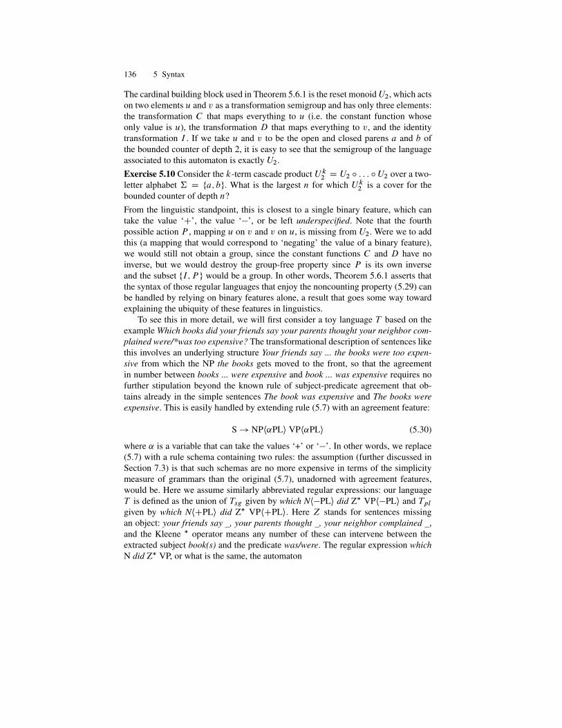
136 5 Syntax

The cardinal building block used in Theorem 5.6.1 is the reset monoidU2, which actson two elements u and v as a transformation semigroup and has only three elements:the transformation C that maps everything to u (i.e. the constant function whoseonly value is u), the transformation D that maps everything to v, and the identitytransformation I . If we take u and v to be the open and closed parens a and b ofthe bounded counter of depth 2, it is easy to see that the semigroup of the languageassociated to this automaton is exactly U2.Exercise 5.10 Consider the k-term cascade product U k

2 D U2 ı : : : ıU2 over a two-letter alphabet † D fa; bg. What is the largest n for which U k

2 is a cover for thebounded counter of depth n?From the linguistic standpoint, this is closest to a single binary feature, which cantake the value ‘C’, the value ‘�’, or be left underspecified. Note that the fourthpossible action P , mapping u on v and v on u, is missing from U2. Were we to addthis (a mapping that would correspond to ‘negating’ the value of a binary feature),we would still not obtain a group, since the constant functions C and D have noinverse, but we would destroy the group-free property since P is its own inverseand the subset fI; P g would be a group. In other words, Theorem 5.6.1 asserts thatthe syntax of those regular languages that enjoy the noncounting property (5.29) canbe handled by relying on binary features alone, a result that goes some way towardexplaining the ubiquity of these features in linguistics.

To see this in more detail, we will first consider a toy language T based on theexample Which books did your friends say your parents thought your neighbor com-plained were/*was too expensive? The transformational description of sentences likethis involves an underlying structure Your friends say ... the books were too expen-sive from which the NP the books gets moved to the front, so that the agreementin number between books ... were expensive and book ... was expensive requires nofurther stipulation beyond the known rule of subject-predicate agreement that ob-tains already in the simple sentences The book was expensive and The books wereexpensive. This is easily handled by extending rule (5.7) with an agreement feature:

S ! NPh˛PLi VPh˛PLi (5.30)

where ˛ is a variable that can take the values ‘+’ or ‘�’. In other words, we replace(5.7) with a rule schema containing two rules: the assumption (further discussed inSection 7.3) is that such schemas are no more expensive in terms of the simplicitymeasure of grammars than the original (5.7), unadorned with agreement features,would be. Here we assume similarly abbreviated regular expressions: our languageT is defined as the union of Tsg given by which Nh�PLi did Z� VPh�PLi and Tpl

given by which NhCPLi did Z� VPhCPLi. Here Z stands for sentences missingan object: your friends say , your parents thought , your neighbor complained ,and the Kleene � operator means any number of these can intervene between theextracted subject book(s) and the predicate was/were. The regular expression whichN did Z� VP, or what is the same, the automaton

5.7 Further reading 137

0which // 1

N // 2did //

Z

��3

VP // 4 (5.31)

will accept the desired language without proper agreement. To get the agreementright, we take the cascade product with the depth 2 bounded counter whose transitionis defined for all clones as the identity mapping for all states and all symbols, exceptNhCPLi will move clone 1 from the initial (accepting) state to the other (warning)state, and for clone 3 the input VPhCPLi will force a move back to the initial state.

What this simple treatment of T shows is that cascade multiplication with a smallreset automaton is sufficient to keep one bit of information around even though anarbitrary amount of material may intervene before we make use of this bit. If wemeasure the complexity of the automaton by the number of states it has, the cas-cade product is very expensive (multiplying with U2 will double the size of the statespace), but by the same general principle that treats (5.7) and (5.30) as having equalor nearly equal cost, a more proper measure of automaton complexity is the numberof states in its cascade decomposition, which increases only linearly in the numberof bits kept around.

5.7 Further reading

Distributional criteria for lexical categorization were advocated by Bloomfield (1926,1933) and elaborated further by Bloch and Trager (1942) and Harris (1951). Defi-nition (1) is known as the Myhill-Nerode equivalence or the syntactic congruenceassociated with a languageL as it was Myhill (1957) and Nerode (1958) who proved,independently of one another, the key theorem that this equivalence, extended to†�,has only finitely many classes iff L is regular. For a modern survey, see Pin (1997).For the use of noncounting in practical grammar design, see Yli-Jyra (2003,2005)and Yli-Jyra and Koskenniemi (2006).

The classical works on categorial grammars are Ajdukiewicz (1935), where thegroup is taken to be Abelian, Bar-Hillel (1953), and Lambek (1958). Some of theinterest in the area was lost when Bar-Hillel, Gaifman, and Shamir (1960) provedthe equivalence of CFGs to one form of categorial grammar, but the field has largelyrevived owing to its strong relation to semantics. The equivalence between CFGs andLambek grammars has been proven by Pentus (1997) – a more accessible proof isgiven in Chapter 3 of Kracht (2003), which presents categorial grammars in greaterdepth.

Although X-bar theory clearly originates with Harris (1951), the name itself isfrom Chomsky (1970) and subsequent work, especially Jackendoff (1977). For amore detailed discussion, see Kornai and Pullum (1990). A good survey of the lin-guistic motivation for going beyond the CF domain is Baltin and Kroch (1989). Theequivalence, both weak and strong, between alternative formulations of extendedphrase structure and categorial systems has been proven in a series of papers byJoshi and his students, of which we single out here Vijay-Shanker et al. (1987) andWeir (1992).

138 5 Syntax

Moravcsik and Wirth (1980) presents the analysis of (5.8) and (5.9) in a varietyof syntactic frameworks. Some of these frameworks are still in use in essentially un-changed format; in particular tagmemics, being the standard theory at the SummerInstitute of Linguistics is in wide use, and covers an immense variety of languages,many of which have no analyses in any other framework. Other frameworks, suchas Montague grammar, relational grammar, and role and reference grammar, havechanged mildly, but the reader interested in a quick overview can still get the ba-sic facts from the respective articles in the Moravcsik-Wirth volume. Yet others, inparticular mainstream transformational theory, have changed so radically that thepresentation of trace theory in that volume is of historical interest only. The readerinterested in more current developments should consult Chomsky (1995) and subse-quent work.

The first proposal within generative linguistics to use case as the driving mecha-nism for syntax was by Fillmore (1968, 1977). The standard introduction to ergativ-ity isDixon (1994). Dependency grammars are due to Tesniere (1959). Other modernformulations include Sgall et al. (1986), Mel’cuk (1988), Hudson (1990), and Mc-Cord (1990). Again, an important early result that served to deflect interest from thearea was by Gaifman (1965), who proved the equivalence of one formulation of de-pendency grammar to CFGs, and again the area revived largely because of its strongconnections to key notions of grammar. A variety of dependency and valency mod-els are surveyed in Somers (1987) and Tapanainen and Jarvinen (1997). A modernsurvey of argument linking theories is Levin and Rappaport (2005).

For linearization of Hayes-Gaifman-style DGs, see Yli-Jyra (2005) and for link-ing a different formulation of DGs to mildly context sensitive grammars and lan-guages see Kuhlmann (2005). The MIL formalization of DG is from Kornai (1987),except there it was given as an equational system in the sense of Curry and Feys(1958 Ch. 1E) rather than stated in the more widely used language of universal al-gebra. The ID/LP analysis of the Dutch crossed dependency is due to Ojeda (1988).The valence (clause) reduction analysis of hate to smoke and similar constructionsoriginates with Aissen and Perlmutter (1983); see also Dowty (1985) and Jacobson(1990).

The method of mapping linguistic expressions to algebraic structures in orderto capture some of their significant properties is not at all restricted to the simpleexamples of checking agreement or slot/filler relations discussed here. The moderntheory of using types as a means of checking correctness begins with Henkin (1950).In type-logical grammar we can use proofnets to check the syntactic correctness ofstrings based on their types (Carpenter and Morrill 2005). Another theory of note,pregroup grammar, uses left and right adjoints to avoid the issues of group elementscommuting with their inverses. Lambek (2004) defines pregroups as partially orderedmonoids where the partial order is compatible with the monoid multiplication, andmultiplication with every element has a left and a right adjoint. His example is the setof Z ! Z functions that are unbounded in both directions, with function compositionas the monoid operation. The relationship of pregroups to categorial grammar and(bi)linear logic is discussed in Casadio et al. (2005).

5.7 Further reading 139

In Minsky’s (1975) theory, the slots are endowed with ranges (used for errorchecking) and often with explicit algorithms that compute the slot value or updateother values on an as-needed basis, but there are no clear natural language phenom-ena that would serve to motivate them. Altogether, the relationship between AI/KRand syntax is far more tenuous today than it was in the 1970s: on the one hand, AI/KRhas largely given up on syntax as too hard, and on the other, its center of gravity hasmoved to machine learning, a field more immediately concerned with linguistic pat-tern recognition in speech, handwriting, and machine print recognition (see Chapters8 and 9) than in syntax proper. For default inheritance and defeasible reasoning, seeGinsberg (1986a). The best introduction to thematic roles remains Dowty (1991).

The complex and often acrimonious discussion that followed Chomsky’s (1957)introduction of arbitrary depth center-embedded sentences led to important method-ological advances, in particular the introduction of the distinction between compe-tence and performance (Chomsky 1965) discussed in Section 3.2. For the debatesurrounding generative semantics, see Newmeyer (1980), Harris (1995), and Huckand Goldsmith (1995).

For the linguistic use of arbitrary semirings for weighted languages, automata,and transducers see Mohri et al (1996), Eisner (2001). The interpretation of theweights as degrees of grammaticality is due to Chomsky (1967). The density of lan-guages was first discussed in Berstel (1973), who considered pairs of languages Land mappings f from†� to RC. He also considered the ratio of the summed weights(summed for strings of length � n in L in the numerator and for all strings in †n inthe denominator), while our definition (see Kornai 1998) uses the differences, segre-gated by sign. We believe that our choice better reflects the practice of computationallanguage modeling, since in these models both underestimation and overestimationerrors are present, and their overall effects are seldom determined in the limit (incor-rect estimates for high-frequency strings are far more important than incorrect esti-mates for low-frequency strings). For natural numbers represented in binary, Minskyand Papert (1966) use density arguments to prove that e.g. the primes in base two arenot regular; see also Cobham (1969) and Chapter 5 of Eilenberg (1974).

The early work on probabilistic FS and CF grammars is summarized in Levelt(1974 Ch. 3). Outside sociolinguistics, probabilistic theories of grammar had little in-fluence because Chomsky (1957) put forward the influential argument that colorlessgreen ideas sleep furiously is grammatical and *furiously sleep ideas green color-less is ungrammatical, yet both have frequency zero, so probability has no traction inthe domain of grammar (for a modern assessment of this argumentation, see Pereira2000). Within sociolinguistics, however, the variability of the data is so overwhelm-ing that there was never a question of abandoning the probabilistic method. The stan-dard introduction to variable rules is Cedergren and Sankoff (1974). The free choicebetween the additive and the multiplicative models has been cogently criticized byKay and McDaniel (1979). Logistic models were introduced to sociolinguistics byRousseau and Sankoff (1978). HMMs as formal models were introduced by Baumand Petrie (1966) and Baum et al. (1970), and first put to significant use in speechrecognition by Baker, Jelinek, and their colleagues at IBM. The standard tutorial in-

140 5 Syntax

troduction is Rabiner (1989); for a more extensive and deeper treatment, see Jelinek(1997). For a detailed discussion of probabilistic CFGs, see Charniak (1993).

The use of formal power series in noncommuting variables to describe ambiguityin CFLs and the concomitant use of semirings originates with Schutzenberger (1960).Early developments are summarized in Chomsky and Schutzenberger (1963). Forthe rational case, see Eilenberg (1974), and for general development of the semiring-oriented approach, see Kuich and Salomaa (1986). For further discussion of Parikhmappings in the weighted case, see Petre (1999). For initial estimates of state spacesize, see Kornai (1985) and Kornai and Tuza (1992) – the estimate we shall derive inSection 6.3.2 also takes ambiguity into account.

For a simple proof of Theorem 5.6.1 see Section 7.12 of Ginzburg (1968), writtenby Albert Meyer – the same ideas are presented in Meyer (1969). The classical studyof this area is McNaughton and Papert (1971), which discusses both the well-knownequivalence of noncounting and star height zero and its relation to temporal logic,also discussed in Maler and Pnueli (1994). For a modern treatment, see Thomas(2003). The idea of a prime minister and a cabinet is based on Bergeron and Hamel(2004), where the important relation between bit-vector operations and noncountinglanguages is explored. For closure of noncounting languages under a relaxed alter-native of Karttunen’s (1995) replacement operator, see Yli-Jyra and Koskenniemi(2006).

A significant source of external evidence, not discussed in the main text as thereis no mathematical treatment in existence, is language pathology. For the pioneeringeffort in this direction, see Jakobson (1941). Chomsky (1965) has distinguished theinternal combinatorical evidence from the broader external considerations discussedhere under the heading of descriptive vs. explanatory adequacy. The pivotal studylinking the extensive literature of child language acquisition to formal theories ofinductive learning is Wexler and Culicover (1980); see also Cussens and Pulman(2001). We shall return to inductive inference in Chapter 7.

As discussed in Chapter 2, grammarians before de Saussure and structuralism didnot hesitate to consider evidence from another source: dialectal and historical varia-tion of the language. Under the influence of de Saussure, such evidence has largelyfallen into disfavor, since it is clear that people can, and do, learn language withoutaccess to such data. The same can be said of evidence from translation: though manylanguage learners benefit from learning two or more languages in early childhood,monolingual language acquisition is obviously possible. Evidence from translationis generally accepted in the form of paraphrases, a method we will discuss furtherin Chapter 6.

6

Semantics

To the mathematician encountering linguistic semantics for the first time, the wholearea appears as a random collection of loosely connected philosophical puzzles, heldtogether somewhat superficially by terminology and tools borrowed from logic. InSection 6.1 we will discuss some of the puzzles that played a significant role in thedevelopment of linguistic semantics from a narrow utilitarian perspective: supposean appropriate technique of mathematical logic can be found to deal with the philo-sophical puzzle – how much does it help us in dealing with the relationship betweengrammatical expressions and their meaning? Since the task is to characterize this re-lationship, we must, at the very least, provide a theory capable of (A) characterizingthe set of expressions and (B) characterizing the set of meanings. By inspecting theLiar (Section 6.1.1), opacity (Section 6.1.2), and the Berry paradox (Section 6.1.3),we will gradually arrive at a more refined set of desiderata, distinguishing those thatwe see as truly essential for semantics from those that are merely nice to have. Thesewill be summarized in Section 6.1.4.

In Section 6.2 we describe the standard formal theory that meets the essentialcriteria. Our point of departure will be Montague grammar (MG) in Section 6.2.1,but instead of formalizing the semantics of a largely artificial and only superficiallyEnglish-like fragment, we set ourselves the more ambitious goal of exploring thesemantics of everyday language use, which tolerates contradictions to a surprisingdegree. In Section 6.2.2, we introduce a version of paraconsistent logic, Ginsberg’s(1986) systemD, and survey the main construction types of English from a semanticperspective.

Finally, in Section 6.3, we begin the development of a formal theory that departsfrom MG in many respects. Our main concern will not be with the use of paracon-sistent/default logic (although we see this as inevitable) but rather with replacingTarski-style induction on subformulas by a strict left-to-right method of building thesemantic analysis. We take this step because induction on subformulas presumes treestructure, while in natural language syntax there are clear technical reasons to preferFSTs, HMMs, and other finite state methods of syntax analysis that do not naturallyendow strings with tree structure.

142 6 Semantics

6.1 The explanatory burden of semantics

While contemporary mathematical logic is indistinguishable from other branches ofmathematics as far as its methods or driving esthetics are concerned, historically ithas grown out of philosophical logic and owes, to this day, a great deal to its orig-inal philosophical motivations, in particular to the desire to eliminate ambiguitiesand paradoxes from the system. From a linguistic perspective, these are questionablegoals since natural language is often ambiguous and clearly capable of expressingparadoxes. What linguistics needs is not a perfect language free of all ambiguity andcontradiction, but rather a meta-theory that is capable of capturing these character-istic properties (we hesitate to call them imperfections, as there is no evolutionarypressure to remove them) of the object of inquiry.

6.1.1 The Liar

Pride of place among the philosophical puzzles readily expressible in natural lan-guage must go to the Liar:

This sentence is false (6.1)

Perhaps the simplest resolution of the paradox would be to claim that the sentence(6.1) is simply not grammatical. But given its structural similarity to sentences suchas This man is asleep, this is not a very attractive claim. A more sophisticated ver-sion of the same argument would use some version of the generative semantics viewintroduced in Section 5.2 and claim that sentence generation starts with some stateof affairs to be put into words, and since there is no conceivable state of affairs corre-sponding to (6.1), the sentence just never gets generated, let alone interpreted. Again,this is not very attractive in the light of the fact that in rather simple contexts (6.1) isperfectly meaningful:

The very first sentence in Fisher’s biography of Lincoln asserts “Abe Lincolnwas born in a log cabin in Idaho”. This sentence is false.

Perhaps one could claim that This in (6.1) must refer to something external to thesentence, but again there is little to support this: examples such asThis sentence is inGerman or This sentence takes 56 characters to print are perfectly ordinary. Sincewe cannot really blame the syntax of (6.1), we need to turn to its semantics. Whatis this referring to? Clearly, it refers to the entire sentence S in (6.1). Therefore, wemay conclude that (6.1) asserts

S is false ^ S D ŒThis sentence is false� (6.2)

The classical solution, Russell’s theory of types, is based on the observation that(6.1) and (6.2) are not the same sentence and not entirely the same assertion. It ispossible to build up a large and useful logical calculus that includes something likea T-scheme (the axiom scheme connecting assertions about the truth of sentences tothe actual truth of sentences – more on this later) while carefully banning only a few

6.1 The explanatory burden of semantics 143

self-referential statements. Here we are interested in a more linguistic solution, onethat does not do away with self-referentiality, since there is no evidence that languagetreats linguistic objects such as words or sentences in any way different from otherabstract nouns. We state this as our requirement (C): expressions that have similarform should receive analyses by the same apparatus.

The central observation is that predicates such as true and false are context-dependent, and in analyzing (6.1) there is no reason to use an eternal absolute notionof truth and falsehood. Since even the most eternal-looking mathematical expres-sions such as 6 � 6 D 36 depend on implicit assumptions (e.g. that of using base 10),there is every reason to suppose that natural language expressions such as (6.1) doalso. Let us call a set of assumptions (closed formulas in a logical language) a contextand denote it by C . If a statement s is true in the context (true in all models that theset of formulas C holds true), we write s 2 T .C /, if false, we write s 2 F.C/ – itis possible for s to be true but be outside the deductive closure of C . Now (6.1) and(6.2) can be reformulated as

S D ŒS 2 F.C/� (6.3)S 2 C ^ S D ŒS 2 F.C/� (6.4)

respectively. Of these, (6.4) is manifestly self-contradictory, which, in an ordinarysystem of two-valued logic, is sufficient cause to declare it false. Kripke (1975) de-velops a three-valued logic with a middle truth value that offers an escape, but wedo not follow this development because the ‘strengthened’ version of the Liar, Thissentence is not true, would cause the same problem to a three-valued treatment that(6.1) causes in a two-valued system. Rather, we follow the Russellian insight and foreach context C define bC as the set of those statements that refer to T .C / or F.C/.Formally, we adjoin a predicate T meaning ‘is true’ to the language and make itsubject to axioms (called the T-scheme in Tarski 1956) such as x , T .x/. Now wecan capture the essence of the ‘naive’ analysis (formalized by Prior 1958, 1961) that(6.1) is not just contradictory, but false:

Theorem 6.1 For every context C; (6.1) is false in bC .

Proof Suppose indirectly S 2 T .bC/. By the T-scheme, we have S 2 F.C/, andtherefore C is a context for S . This, by S , leads to S 2 T .C /, a contradiction thatproves that our indirect assumption was false.

Discussion This is not to say that the Liar is not a valuable paradox: to the contrary, inthe history of logic, the Liar and closely related paradoxes such as the barber paradoxhave led to many notable advances in logic, including Russell’s theory of types andTarski’s undefinability theorem. However, from a linguistic perspective many of theissues brought up by the Liar are already evident in much simpler nonparadoxicalsentences that have no self-referential or quotational aspect whatsoever. First, andmost important, is the treatment of nonintersective modifiers. At the very least, we

144 6 Semantics

need a theory that covers enormous flea (Parsons 1970) and lazy evaluation beforewe can move on to false sentence.1

Once such a theory is at hand (and as we shall see, this is by no means a trivialtask), there is the further question of whether we really need a linguistic semanticaccount of true and false. English, as a formal language, contains many expressionswith these words, but formal semantics generally refrains from the explication ofordinary nouns and adjectives like flea and enormous, preferring to leave such mat-ters either to specialists in biology and psychology or to lexicographers and knowl-edge representation experts. There is no compelling reason why sentence and trueshould occupy a more central position in our development of semantics: we con-clude that for the purposes of linguistic semantics an analysis of these notions is nicebut inessential. On the other hand, since self-referential statements are formed byordinary grammatical means, it follows from (C) that we should cover them.

Quotational sentences are also problematic from our perspective. Our intona-tional means to segregate quoted from direct material are limited: a sentence such as‘Snow is white’ is true if and only if snow is white is practically impossible to renderdifferently from ‘Snow is white’ is true if and only if ‘snow is white’. Since we areattempting a formal reconstruction, a general appeal to the universality of naturallanguage, (i.e. to the notion that everything can be discussed in natural language) isinsufficient – what we need is a precise mechanism whereby matters such as quota-tion can be discussed. The use of quotation marks in written language provides thebeginnings of such a mechanism, but as far as grammar is concerned these are notvery well regulated, especially when it comes to quotations inside quotations beyonddepth two. And even without embedding, the matter is far from trivial: compare A‘quine’ is a program that, when compiled and executed, prints its own source codeto A quine is a program that, when compiled and executed, prints its own sourcecode. We conclude that a theory of quotation is nice but inessential, especially as thephenomenon is more characteristic of artificially regulated written communicationthan of natural language.

6.1.2 Opacity

Another important puzzle is that of opacity (used here in a very different sense fromthat in phonology or syntax). It has long been noted that certain predicates P aboutstatements s and t do not allow for substitution. Even if s D t it does not follow thatP.s/ D P.t/. Frege (1879) used know as an example of such a predicate, but theobservation remains true of many other predicates concerning knowledge, (rational)belief, hope, preference, (dis)approval, etc., generally collected under the headingof propositional attitudes. Frege used as his example the knowledge state of ancientGreeks, who had not realized prior to Pythagoras that Hesperus (the evening star),and Phosphorus (the morning star) were one and the same object, what we call Venus

1 What is common to the examples is that enormous fleas are not enormous things that arealso fleas (hence the name nonintersective), lazy evaluation is not some lazy thing that hap-pens to be an evaluation, and true sentences are not true things that happen to be sentences.

6.1 The explanatory burden of semantics 145

today. Thus, for an ancient Greek it was perfectly possible to know/believe that abright object in the evening sky is Hesperus without knowing/believing that it isPhosphorus. In other words, Believe(s) does not follow from Believe(t) even thoughs D t .

In the tradition of philosophical logic, opacity is intimately linked to a priori,analytic, and necessary statements, and for those whose goal is to develop rationaltheories of beliefs, propositional attitudes, and judgments in general, such consider-ations are valuable. But from our perspective, the issue is nearly trivial: there is nodenying that (i) sentences about beliefs, etc., are about the mental states of peopleand that (ii) mental models need not correspond to facts. The ancient Greeks had amodel of the world in which there were two different entities where in reality therewas only one. In other cases people, or entire civilizations, assume the existenceof entities that do not correspond to anything in reality (the Western philosophicaltradition generally exemplifies this by unicorns) or conversely use models that haveliterally no words for important entities. But imperfect knowledge and mistaken be-liefs are part of the human condition: there is no logical error, and what is moreimportant here, there is no grammatical error in thinking or saying things that arenot so. Again, from a linguistic perspective the issues brought up by opacity are ev-ident in much simpler cases that do not probe the edges of logical, philosophical, orphysical necessity: ordinary fiction will suffice. What do we mean when we say AnnaKarenina is afraid of getting older? How does it differ from Jean Valjean is afraidof getting older? Most people will agree that Anna Karenina commits suicide is trueand Jean Valjean commits suicide is false. It is a highly nontrivial task to design atheory that provides the expected results in such cases, and although the desideratumfollows from (C) it is worth stating it separately: (D) expressions occurring in fic-tion should receive analysis by the same apparatus as expressions used in nonfictioncontexts.

6.1.3 The Berry paradox

In Section 1.5, we already alluded to the Berry paradox of finding

the smallest integer not definable in k words (6.5)

For k � 7 the paradox is not apparent: we enumerate definitions of integers e.g. inlexicographic order, rearrange the list in increasing order of the numbers defined,and pick the first integer not on the list, say sk . But for k D 8 there is a problem:(6.5) itself is on the list, so s8 is defined by it, and we must pick s8 C 1 (or, if itwas defined elsewhere on the list, the next-smallest gap). But then, s8 was not onthe list, or was it? What makes this question particularly attractive is that desiderata(A) and (B) appear to be easily met: it looks trivial to define the syntax of numbernames and, for once, we have a well-agreed-upon semantic model of the domain.There are some core elements one, two, ..., nine that combine with other base tencore elements such as ten, twenty, ..., ninety and hundred, thousand, million, billion,trillion, quadrillion, ... all contributing to the comma-separated reading style (CSRS)

146 6 Semantics

whereby 450,789,123,450,123 is read off as four hundred and fifty trillion seven hun-dred and eighty nine billion one hundred and twenty three million four hundred andfifty thousand one hundred and twenty three. There is something of a performanceissue in where to terminate the sequence: clearly, numbers such as septendecillionor nonillion only serve as party amusements, as the people who actually would needthem will in real life switch over to scientific reading style (SRS) somewhere around109. Once we have made a choice where to terminate the sequence, it is trivial to de-fine a small finite automaton generating all and only the CSRS numbers and anotherautomaton generating SRS numbers such as three point two seven five times ten tothe minus nineteenth.Exercise 6.1 Write a detailed grammar of the CSRS and SRS systems. Make surethat articles are correctly generated both in the conventional listing of numbers one,two, � � �, ninety-nine, one hundred, one/a hundred and one, one/a hundred and two,� � �, two hundred, two hundred and one, � � � and before round numbers. Define theappropriate notion of roundness. Consider grammatical responses to questions suchas How many students are in this school?, explain why *hundred is ungrammaticaland (exactly) one/a hundred are acceptable.

Yet no sooner than we start specifying the syntax beyond these trivial fragmentswe run into difficulties. First, there is no one-to-one relationship between numbersand expressions composed entirely of number names: seven thirty generally refersto a time of the day, nine eleven to emergency services, and forty fifty or two threethousand to approximate quantities given by a confidence interval. This last class isso similar to CSRS that on occasion the lines between the two are blurred: ninetynine hundred can refer both to 9,900 and to 99–100. To be sure, in the written lan-guage hyphens are used with approximate quantities, but spoken English (which forthe linguist has methodological primacy) shows no sign of this. When viewed fromthe perspective of spoken language, the whole enterprise of assigning semantics toCSRS and SRS is of dubious character: such numbers form highly stylized and regu-lated formal languages whose regulatory principles appear to be arithmetical, ratherthan linguistic, in nature. Arithmetic is not acquired with the same effortless easeas a first language. For most people the process starts later, and for many it remainsincomplete.

To get the Berry paradox really working we also need our syntax to cover arith-metic expressions (eight cubed is a number expressible in two words instead of thefour required by CSRS), other bases (hex a a b nine only requires five words), theability to solve equations (the smallest Mersenne prime with an eight digit exponent)and in general to run algorithms (the result of running md5sum on the empty file).Unfortunately, as a technical device for the description of algorithms yielding a nu-merical output, natural language is spectacularly inadequate, requiring a variety ofsupport devices such as end markers, quotation marks, and parentheses, which havelittle or no use in ordinary language, a fact that is painfully evident to anyone whohas ever tried to debug source code over the phone. This makes writing a grammarthat meets (A) a complex matter, as there is no easy test of whether an expressionevaluates to a numerical value or not.

6.1 The explanatory burden of semantics 147

At the same time, when it comes to expressions with a numerical value, natu-ral language overgenerates in two significant ways. First, there are a class of state-ments that become true just by means of saying so, and such statements can be usedto define numbers. To illustrate the more general phenomenon, consider whether astatement such as I promise to come tomorrow can be false. I can break the promise(by not coming), but merely by saying I promise I have actually promised that I willcome. There is a whole set of verbs such as declare, order, request, warn, and apol-ogize that are similarly self-fulfilling – following Austin (1962), these are known asperformatives. The only near-performative in mathematical usage is let: when wesay Let T be a right triangle, T is indeed a right triangle. Compared with the per-formatives in everyday language, the power of let is rather limited. In particular, bysaying things such as let x be a prime between 8 and 10, we have not succeeded increating such a prime, while by saying I name this ship Aoxamoxoa one can indeedcreate a ship by that name. But in the subdomain of naming numbers, the full powerof let is at our disposal: there are monomorphemic elements such as eleven, twelve,dozen in broad use, and others such as gross, score, chiliad, and crore known only tochiliads or perhaps crores of people. As examples such as googolplex show, all thatis required for a successful act of naming is that the language community agrees thata word means a certain thing and not something else. The word factoriplex does notexist in current English but is easily defined as the product of all integers from 1 togoogolplex, minus 42. Performatives trivialize the Berry paradox (there is no numbermeeting (6.5) since every number is nameable in one word) but yield another strongdesideratum: (E) the system must be flexible about naming.

Second, natural language offers a wealth of algorithmic descriptions of numbersthat are solvable only by encyclopedic knowledge. Clearly, the year Columbus dis-covered America evaluates to 1492, and equally clearly, knowing this is beyond thepower of linguistic semantics. As far as the expression is concerned, it could refer toany year within Columbus’ adult life, and no amount of understanding English willsuffice to better pin down the exact date. But if we are reluctant to impute knowl-edge of medieval history to speakers of English, we should be equally reluctant toimpute knowledge of Mersenne primes, or even knowledge of eight cubed. Ratherthan stating this as a negative desideratum, “the system should not rely on exter-nal knowledge”, we state it as a positive requirement: (F) the system must remaininvariant under a change of facts.

The remarks above are not meant to demonstrate the uselessness or irrelevance ofthe Berry paradox (which remains a valuable technical tool e.g. in Kolmogorov com-plexity; see Chapter 7) but rather to make clear that from the standpoint of linguisticsthe difficulties arise long before the diagonalization issues that are in the focus of thelogical treatment would come to force. If we exclude the arbitrariness of numbernaming, references to encyclopedic knowledge, and the description of algorithms,what remains is some extension of the CSRS and SRS grammars. For these, (6.5)has a solution: we run the grammar, evaluate each expression, and pick the smallestone missing from the list of numbers so generated. The paradox disappears since thisamounts to describing an algorithm rather than naming a number.

148 6 Semantics

The hangman paradox

It is possible to interpret the Berry paradox in another manner: consider Your obli-gation will be fulfilled only when you give Berry half of the money in your pocket.A reasonable person may conclude that if he gives Berry half of the money in hispocket, his obligation is fulfilled. However, Berry may object, noting the amount ofmoney still in the person’s pocket, that the obligation is unfulfilled and demand an-other halving, another, and another, ad infinitum. Or consider To complete this task,you need to sleep on it and you must report back to Berry that you are absolutelycertain it’s done. The next day, you may entertain doubts. Since you have not so farreported back to Berry, you have not completed the task, and you need to sleep onit. This interpretation, traditionally presented under the name hangman paradox, hasless to do with finding the smallest solution to (6.5) than with the more wide-rangingproblem of imperatives that demand the impossible. There is nothing on the surfaceto distinguish these from imperatives that can in fact be met. A perfectly analogousproblem is presented by questions that cannot be answered. For any given question,we do not know in advance whether an answer exists, and if we permit a questionto be formulated in a sublanguage that is strong enough to refer to algorithmicallyundecidable issues, we know that some questions will not have answers. Again, thereis no need to probe the edges of undecidability; ordinary adjectival modification willalready furnish plenty of examples such as prime between eight and ten that receiveno interpretation in any model, and embedding such references to impossible objectsin questions or imperatives is a trivial matter. Carefully crafted realist fiction createsa world that appears possible, but to the extent that human language use, and in-deed the whole human condition, is greatly impacted by narratives that defy rationalbelief, requirement D needs to be further strengthened: (G) all expressions shouldreceive analysis by the same apparatus as supposed statements of fact.

6.1.4 Desiderata

Let us now collect the requirements on linguistic semantics that have emerged fromthe discussion. (A) asks for a characterization of the set of natural language expres-sions. In mathematical linguistics, this is done by generating the set (see Section 2.1),and in the previous chapters we have discussed in detail how phonology, morphol-ogy, and syntax, taken together, can provide such a characterization. (B) asks thesame for the set of meanings, but our lack of detailed knowledge about the internalcomposition of the mental form that meanings take gives us considerable freedom inthis regard: any set that can be generated (recursively enumerated) is a viable candi-date as long as it can be used in a theory of semantics that meets the other desiderata.One particularly attractive approach is to represent meanings by well-formed formu-las in some logical calculus, but other approaches, such as network representations,also have a significant following.

Requirement (C), that expressions similar in form should receive analyses bythe same apparatus, has far-reaching consequences. First, it implies a principle ofhomogeneity: to the extent meanings are typed, and this will be necessary at least

6.1 The explanatory burden of semantics 149

to distinguish objects from statements, questions, and imperatives, (C) calls for ex-pressions of the same linguistic type to be mapped on meanings of the same logicaltype. Second, to the extent the meanings of expressions are built recursively from themeanings of their constituents, (C) calls for direct compositionality in the form ofsome rule to rule hypothesis: each step in generating the expression must be pairedwith a corresponding step in generating the meaning. Third, to the extent that thetruth, consistency, feasibility, adequacy, or even plausibility of an expression cannotbe fully known at the time it is uttered, (C) implies our (D) and (G): the meaning ofexpressions is independent of their status in the real world.

In model-theoretic semantics, the meaning representations (formulas) are justtechnical devices used for disambiguating expressions with multiple meanings. Sincethe formulas themselves are mapped onto model structures by an interpretation func-tion, the step of mapping expressions to meanings can be composed with the inter-pretation function to obtain a direct interpretation that makes no reference to theintermediary stage of formulas. In this setup, requirement (F), that the system mustremain invariant under a change of facts, is generally taken to mean that the inter-pretation function is symmetrical (invariant under any permissible permutation ofmodels). But (F) is asking for a considerably more fluid view of facts than what isgenerally taken for granted in model-theoretic semantics: from our perspective, thefact that eight cubed and hex two hundred are the same number, decimal 512, is anentirely contingent statement, perhaps true in some models where correct arithmeticis practiced but quite possibly false in others.

Exercise 6.2 From an early age, Katalin was taught by her older brother that threeplus five is eight, except for chipmunks, where three chipmunks plus five chipmunksare nine chipmunks because chipmunks are counted differently. Two plus two isfour, except for chipmunks, where it is five. One plus one plus one is three, exceptfor chipmunks, where it is five. By age five, Katalin mastered both regular additionand multiplication and chipmunk arithmetic up to about a hundred. Describe hersemantics of arithmetic expressions.

Finally, let us call attention to an important consequence of the mundane treatment ofarithmetic expressions assumed here. In his discussion of Montague (1963), Thoma-son (1977) argues that any direct theory of propositional attitudes is bound to becaught up in Tarski’s (1935) theorem of undefinability (Tarski 1956), rendering theresulting analysis trivial. However, as Thomason is careful to note, the conclusionrests on our ability to pass from natural language to the kinds of formal systemsthat Tarski and Montague consider: first order theories with identity that are strongenough to model arithmetic. Tarski himself was not sanguine about this: he held thatin natural language “it seems to be impossible to define the notion of truth or even touse this notion in a consistent manner and in agreement with the laws of logic”.

To replicate Tarski’s proof, we first need to supplement natural language withvariables. The basic idea, to formalize the semantics of a predicate such as subjectowns object by a two-place relation �.s; o/ is fairly standard (although, as we shallsee in Section 6.3, there are alternatives that do not rely on variables at all). But theproposed paraphrases for first-order formulas, such as replacing 8xŒ9y�.x; y/ !

150 6 Semantics

9z�.z; x/� by for everything x, either there is not something y such that x owns y orthere is something z such that z belongs to x clearly belong in an artificial extensionof English rather than English itself. Second, we must assume that the language cansustain a form of arithmetic; e.g. Robinson’s Q. We have already expressed doubts asto the universality of natural language when it comes to logical or arithmetic calculi,but using Q we can narrow this down further: several of the axioms in Q appearuntenable for natural language. Again, the key issues arise long before we considerexponentiation (a key feature for Godel numbering) or ordering. Q comes with asignature that includes a successor s, addition +, and multiplication �. By Q2 wecan infer x D y from sx D sy, Q4 provides x C sy D s.x C y/, and Q6 givesx � sy D xy C x. All of these axioms are gravely suspect in light of the noncountingprinciple discussed in Section 5.5. There are many ways we can start counting innatural language: we can look at quotations of quotations (Joe said that Bill said...)and emphasis of emphasized material (very very...), but there isn’t a single way thattakes us very far – whichever way we go, we reach the top in no more than four steps,and there Q2 fails.

Since this is one of the key points where the semantics of natural language ex-pressions parts with the semantics of mathematical expressions, it is worth highlight-ing a consequence of the position that worlds, or models (from here on we use thetwo terms interchangeably), need not be consistent: our desideratum (E), that the sys-tem must be flexible about naming, now comes for free. In the following, we employparaconsistent logic to make room for entities such as unicorns, triangular circles,and numbers that remain unchanged after adding one. As readers familiar with mod-ern philosophical logic will know, the use of paraconsistent logic opens the way tonew solutions to the Liar and several other puzzles, but we will not pursue thesedevelopments here – rather, we will concentrate on problems that we have earlieridentified as central, most notably the distinctions between essential and accidentalproperties introduced in Section 5.3.

6.2 The standard theory

In a series of seminal papers, Montague (1970a, 1970b, 1973, all reprinted in Thoma-son 1974) began the development of a formal theory that largely meets, and in somerespects goes beyond, the desiderata listed above. In Section 6.2.1 we introduce thisfamily of theories, known today as Montague grammar (MG). As there are severalexcellent introductions to MG (see in particular Dowty et al. 1981 and Gamut 1991),we survey here only the key techniques and ideas and use the occasion to highlightsome of the inadequacies of MG, of which the most important is the use of a stilted,semiformalized (sometimes fully formalized) and regimented English-like sublan-guage more reminiscent of the language use of logic textbooks than that of ordinaryEnglish. Linguists brought up in a more descriptive tradition are inevitably struck bythe stock examples of MG like Every man loves a woman such that she loves him orJohn seeks a unicorn and Mary seeks it. While still avoiding the rough and tumble ofactual spoken English, we take the object of inquiry to be a less regimented language

6.2 The standard theory 151

variety, that of copyedited journalistic prose. Most of our examples in Section 6.2will be taken from an American newspaper, the San Jose Mercury News. For reasonsof expository convenience, we will often considerably simplify the raw examples,indicating inessential parts by [] wherever necessary, but in doing so, we attempt tomake sure the simplified example is still one that could be produced by a reasonablewriter of English and would be left standing by a reasonable copy editor.

6.2.1 Montague grammar

In Chapter 3, we defined signs as conventional pairings of sound and meaning andelaborated a formal theory of phonology capable of describing the sound aspect ofsigns. Developing a formal theory of semantics that is capable of describing themeaning aspect of signs will not proceed quite analogously since in phonology wecould ignore the syntax, while in semantics it is no longer possible to do so.

The central idea of Montague (1970a) was to introduce two algebras, one syn-tactic and the other semantic, and treat the whole issue of linguistic semantics asa homomorphism from one to the other. As there are several minor technical dif-ferences in the way this idea was implemented in Montague’s main papers on thesubject (and subsequent research has not always succeeded in identifying which ofthe alternatives is really the optimal one), we will not remain meticulously faithfulto any of the founding papers, but we will endeavor to point out at least the mainstrands of development in MG, which, construed broadly, is clearly the largest andmost influential school of contemporary linguistic semantics.

As usual, an algebra is a set T endowed with finitely many operationsF1; : : : ; Fk

of fixed arity a1; : : : ; ak . By an operation of arity a, we mean a function T a ! T , soby convention distinguished elements of the algebra are viewed as nullary operations.For Montague, the syntactic algebra is strongly typed but otherwise unrestricted: ifp and q are expressions of types (categories) P and Q, an operation f will always(and only) produce an expression f .p; q/ of type R. In practice, Montague alwaysused binary operations (a tradition not entirely upheld in subsequent MG work) andwas very liberal as to the nature of these, permitting operations that introduce ordrop grammatical formatives and reorder the constituents. Some later work, such asCooper (1975) or McCloskey (1979), took advantage of this liberal view and per-mitted generative transformations as syntactic operations, while others took a muchstricter view, permitting only concatenation (and perhaps wrapping; see Bach 1981).Either way, the syntactic and semantic algebras of MG provide the characterizationof natural language expressions and meanings required by our desiderata (A) and(B).

The mapping � from the syntactic algebra to the semantic algebra must be ahomomorphism: for each operation f of arity a in the syntactic algebra, there mustbe a corresponding operation g of the same arity in the semantic algebra, and ifr D f .p; q/, we must have �.r/ D g.�.p/; �.q//. While in practice Montague usedformulas of a higher-order intensional logic called IL as elements of the semanticalgebra, with function composition (including applying an argument to a function)as the chief operation, it is clear from his work that he took a far more abstract

152 6 Semantics

view of what can constitute a proper semantic representation. In particular, the ILformulas are interpreted in model structures by another function , which is alsoa homomorphism, so that the �-calculus formulas, viewed by Montague as a merepedagogical device, can be dispensed with entirely, interpreting natural languageexpressions directly in model structures. Later work explored several other choicesfor semantic algebra: Heim (1982) used file change potentials, Cresswell (1985) usedstructures that preserve a record of the way the expression was built up, and manyother options are available, as long as the ultimate model-theoretic nature of theenterprise is preserved (i.e. the structures of the semantic algebra are interpreted inmodels).

Montague used IL first as a means of resolving issues of opacity. Instead of takingthe meaning of terms to be their extension, the set of objects to which the interpreta-tion function maps them in a single model structure, he chose to explicate meaningsas intensions, the set of extensions in all modally accessible worlds. Since the ex-tension of expressions may coincide (for example, in realis worlds both the king ofFrance and the king of Austria denote the empty set), it is not evident how to expressthe clear meaning difference between John aspires to be the king of France and Johnaspires to be the king of Austria or even John aspires to be a unicorn.

With intensions, the problem is solved: since it is easy to imagine an alternativeworld where the French Revolution still took place but Austria, just like Belgium,retained the institution of monarchy, the intension of the two terms is different and wecan ascribe the different meanings of the whole expressions to the different meaningsof the NPs king of France vs. king of Austria. In MG, verbs denoting propositional orother attitudes are called intensional since they operate on intensions: their use solvesmany subtle interpretation problems already known to the Schoolmen, such as the insensu composito/in sensu diviso readings of I want a new car, which may expressthat the speaker has her eye on a particular car or that she wants to replace the oldone with a new one and it does not really matter which one. A similar treatment isavailable for intensional nouns such as temperature: by taking these to be functionsthat take different values in different possible words, we avoid concluding thirty isrising from the temperature is thirty and the temperature is rising.

One problem that this otherwise very satisfactory theory leaves open is knownas the issue of hyperintensionals: there are expressions like prime between 8 and10 and triangular circle that denote empty sets in every modally accessible world;indeed, under most theories of the matter, in any world whatsoever. Clearly, Pappussearched for a method to trisect any angle presumes very different truth conditionsfrom Pappus searched for a method to square the circle even if, in hindsight, it isclear that the two activities are equally futile.

Another technical device of MG worthy of special mention is the use of disam-biguated language. Since � (or � ı / is a function, only a single translation canattach to any expression, so those expressions that are ambiguous need to be as-signed as many disambiguated versions as there are separate meanings. In syntax,the preferred method of disambiguation is by constituent structure, as in [The manon the hill] with the telescope as opposed to The man on the [hill with the telescope].In semantics, however, we often find cases like (5.2), where the constituent struc-

6.2 The standard theory 153

ture is unambiguous, Every man [loves a woman], yet the sentence has two distinctreadings, (5.3) and (5.4), corresponding to the order in which the universal every andthe existential a get to bind the variables in loves(x,y). We can use derivation his-tory to distinguish such cases: the same constituent structure is reached by applying(possibly different) operations in different orders.

To see how the ambiguity is handled in MG, we need to consider another char-acteristic feature of MG, the use of generalized quantifiers. Intuitively, individuals(proper nouns such as John or NPs such as the dog) should be interpreted as ele-ments of model structures (type e), and properties (be they expressed adjectivally:(is) red, (is) sleepy; or by intransitive verbs: sleeps) are interpreted as functions fromindividuals to truth values (type e ! t ). Yet quantified NPs, such as some men,every dog, no tree, etc., are syntactically congruent to simple NPs such as John orthe dog, and our desideratum (C) demands that they should receive analysis by thesame apparatus as these. Since quantified NPs can be easily conceptualized as setsof properties (those properties, be they essential or accidental, that are shared by allmembers of the set), we lift the type of simple NPs from e to .e ! t / ! t andconceptualize them as the set of all properties enjoyed by the individual. Once thisstep is taken, the intuitive assignment of sleeps as function and John as argumentcan (indeed, must) be reversed for the function application to come out right. Thetranslation of every man is �P.8x.man.x/ ! P.x///, so that translation of Everyman sleeps is obtained by applying this function to the translation of sleeps, yielding(by beta conversion) the desired 8x.man.x/ ! sleep.x//:

Similarly, a woman is translated �P.9x.woman.x/ ! P.x///, and if loves istranslated as a two-place relation l.x; y/, loves a woman will be 9y.woman.y/ !

l.x; y//. Some care must be taken to make sure that it is the second (object of love)variable that is captured by the existential quantifier, but once this is done, the resultis again an e ! t function ready to be substituted into �P.8x.man.x/ ! P.x///,yielding 8x.man.x/ ! 9y.woman.y/ ! l.x; y///, the reading given in (5.3).In Montague’s original system, the other reading (5.4), 9y.woman.y/8x.man.x/l.x; y/// is obtained by radically different means: by introducing, and later deleting,a variable that is viewed as being analogous to a pronoun.

From here on, we do not follow Montague closely, since our primary concern iswith natural language rather than with the semiformalized (sometimes fully formal-ized) and regimented English-like sublanguages used in most works of philosophicallogic. In everyday usage, as evidenced e.g. by newspaper texts, quantified NPs suchas every Californian with a car phone, every case, every famous star, etc., do notlend themselves to a strict interpretation of every x as 8x inasmuch as they admitexceptions: every case, except that of Sen. Kennedy; every Californian with a carphone, except drivers of emergency vehicles; every famous star, including Benji, etc.The problem, known as the defeasability of natural language statements, has givenrise to a wide variety of nonmonotonic logic approaches (for an overview see Gins-berg 1986a). Of particular interest here are generic constructions such as Sea turtleslive to be over a 100 years old, which can be true even if the majority of specificinstances fail. At the extreme end, some generic statements such as P6 processorsare outdated may be considered true without any individual instances holding true.

154 6 Semantics

We define a construction as a string composed of nonterminals (variables rang-ing over some syntactic category) and terminals (fixed grammatical formatives andlexical entries) with a uniform compositional meaning, obtained by a fixed processwhose inputs are the meanings of the nonterminals and whose output is the meaningof the construction as a whole. An example we saw in Section 5.3 was X is to Y asZ is to W, but we use the term here in the general linguistic sense, which covers theentire range from completely productive and highly abstract grammatical patternssuch as

NPh˛PERS ˇNUMi VPh˛PERS ˇNUM TENSEi (6.6)

to highly specified and almost entirely frozen idioms such as

NPh˛PERS ˇNUMi kickh˛PERS ˇNUM TENSEi the bucket (6.7)

On occasion, when we are interested in the substitution of one construction intoanother, it will be necessary to assign a grammatical category (defined as includ-ing morphosyntactic features specified in angled brackets) to the construction as awhole, so a context free or mildly context-sensitive theory of constituent structure(see Section 5.1.3) roughly along the lines of GPSG (Gazdar et al. 1985) or earlyHPSG (Pollard 1984) is presupposed. For the purposes of this chapter, we can safelyignore transference across patterns, such as the phenomenon that the agreement por-tion of (6.7) is obviously inherited from that of (6.6), and concentrate more on thesemantics of constructions.

As a limiting case, entirely frozen expressions (i.e. those constructions that nolonger contain open slots, such as go tell it to the Marines) are simply taken as lexi-cal entries; in this case, with meaning ‘nobody cares if you complain’. (The indexi-cals implicit in the imperative go and explicit in the paraphrased you do not constituteopen slots in the sense that interests us here.) Since compositionality cannot be main-tained as a principle of grammar without relegating the noncompositional aspects ofconstructions to the lexicon, we introduce the following Principle of Responsibility:The semantics of any expression must be fully accounted for by the lexicon and thegrammar taken together. To make this principle clear, consider constructions such as

for all NPh+DEFi, S (6.8)

as in the following examples: For all the glamour of aerial fish planting, it was amass production money-maker; The Clarence Thomas hearings, for all their import...or For all their efforts at parity and fairness, NFL officials .... Informally, the con-struction means something like ‘S , in spite of the usual implications of NPh+DEFi’.In the case of the glamour of aerial fish planting, the implication that needs to bedefeased is that glamorous things are restricted to the few, a notion incompatiblewith mass production. Thus, to make sense of (6.8), we need to rely on lexical in-formation. Without doing so, the clear difference between the acceptability of thepreceding examples and ???For all their protein content, eggs are shaped so as toease passage through the duct would remain completely mysterious.

6.2 The standard theory 155

Since universally quantified natural language NPs can actually have exceptions,we need to capture the notion of exceptionality some way; e.g. by saying that En-glish every man means ‘almost all men’ in the sense that exceptions have measurezero. Unfortunately, there is no obvious way to define measure spaces over seman-tic objects such as legal cases or California drivers with car phones naturally, soto translate Geraldo Rivera [reveals that he is an extremely attractive virile hunk ofman who] has had sex with [] every famous star in the entertainment industry wesay that for all x such that x has no extra properties beyond being a famous star inthe entertainment industry, Geraldo Rivera has had sex with x.

A less clumsy translation, in keeping with the standard treatment of generalizedquantification, is to say that the property of having had sex with Geraldo Rivera isimplied by the property of being a famous star in the entertainment industry. We saythat every N is the set of typical properties that N has, where typicality is defined inthe lexical entry ofN . Since having four legs is typical of donkeys, every donkey hasfour legs will be true by definition and cannot be falsified by the odd lame donkeywith three or fewer legs.

But if having four legs is an analytic truth for donkeys, how can we account forcounterfactuals where five-legged donkeys can appear easily, or for the clear intuitionthat being four-legged is a contingent fact about donkeys, one that can be changede.g. by genetic manipulation? The answer offered here is that to reach these we needto change the lexicon. Thus, to go from the historical meaning of Hungarian kocsi‘coach, horse-driven carriage’ to its current meaning ‘(motor) car’, what is needed isthe prevalence of the motor variety among ‘wheeled contrivances capable of carryingseveral people on roads’. A 17th century Hungarian would no doubt find the notionof a horseless coach just as puzzling as the notion of flying machines or same-sexmarriages. The key issue in readjusting the lexicon, it appears, is not counterfactual-ity as much as rarity: as long as cloning remains a rare medical technique, we willnot have to say ‘a womb-borne human’.

To summarize our main departure from standard MG: under the treatment as-sumed here, every man loves a woman means neither (5.3), 8xman.x/ 9ywoman.y/loves.x; y/ nor (5.4), 9ywoman.y/ 8xman.x/ loves.x; y/; it means that woman-loving is a typical property of men, just as donkey-beating is a typical property offarmers. Some of the typical properties of common nouns are analytic relative to agiven lexicon while others are not. In fact, for every noun there are only a handful ofdefining properties (see Section 5.3), and these can change with time in spite of theinherent conservatism of the lexicon.

Ordinary adjectival modification means conjoining another property to the bun-dle (conjunction) of essential properties, so brown dog refers to the conjunction of allessential dog properties and brownness. Enormous fleas have the property of enor-mity conjoined to the essential properties of fleas, which include being rather small,so the notion is applied, without any special effort, on the flea scale. The same simpletreatment is available for impossible objects such as triangular circles.

Figure 6.1 shows on the left a slightly triangular circle and on the right a slightlycircular triangle. Whether the object in the middle, known as the Reuleaux triangle,is considered a triangle, a point of view justified by its having three distinct vertices,

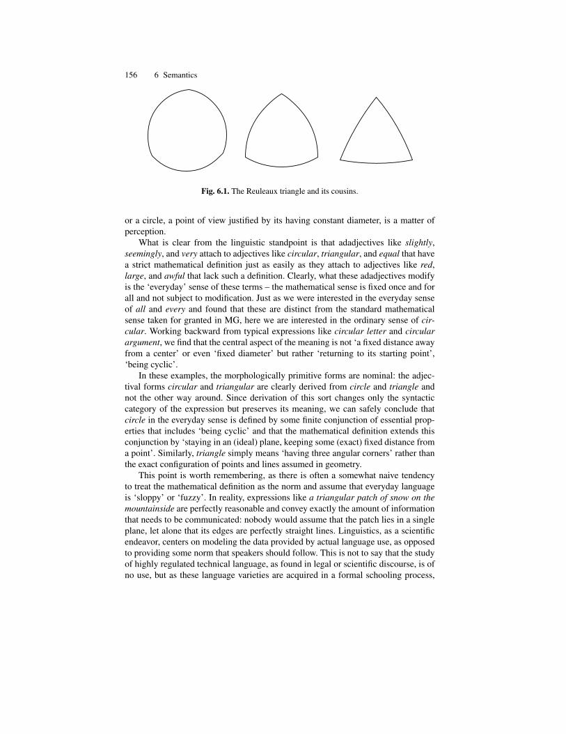
156 6 Semantics

Fig. 6.1. The Reuleaux triangle and its cousins.

or a circle, a point of view justified by its having constant diameter, is a matter ofperception.

What is clear from the linguistic standpoint is that adadjectives like slightly,seemingly, and very attach to adjectives like circular, triangular, and equal that havea strict mathematical definition just as easily as they attach to adjectives like red,large, and awful that lack such a definition. Clearly, what these adadjectives modifyis the ‘everyday’ sense of these terms – the mathematical sense is fixed once and forall and not subject to modification. Just as we were interested in the everyday senseof all and every and found that these are distinct from the standard mathematicalsense taken for granted in MG, here we are interested in the ordinary sense of cir-cular. Working backward from typical expressions like circular letter and circularargument, we find that the central aspect of the meaning is not ‘a fixed distance awayfrom a center’ or even ‘fixed diameter’ but rather ‘returning to its starting point’,‘being cyclic’.

In these examples, the morphologically primitive forms are nominal: the adjec-tival forms circular and triangular are clearly derived from circle and triangle andnot the other way around. Since derivation of this sort changes only the syntacticcategory of the expression but preserves its meaning, we can safely conclude thatcircle in the everyday sense is defined by some finite conjunction of essential prop-erties that includes ‘being cyclic’ and that the mathematical definition extends thisconjunction by ‘staying in an (ideal) plane, keeping some (exact) fixed distance froma point’. Similarly, triangle simply means ‘having three angular corners’ rather thanthe exact configuration of points and lines assumed in geometry.

This point is worth remembering, as there is often a somewhat naive tendencyto treat the mathematical definition as the norm and assume that everyday languageis ‘sloppy’ or ‘fuzzy’. In reality, expressions like a triangular patch of snow on themountainside are perfectly reasonable and convey exactly the amount of informationthat needs to be communicated: nobody would assume that the patch lies in a singleplane, let alone that its edges are perfectly straight lines. Linguistics, as a scientificendeavor, centers on modeling the data provided by actual language use, as opposedto providing some norm that speakers should follow. This is not to say that the studyof highly regulated technical language, as found in legal or scientific discourse, is ofno use, but as these language varieties are acquired in a formal schooling process,

6.2 The standard theory 157

over many years of adult study (as opposed to the acquisition of natural language,which takes place at an earlier age and generally requires no schooling whatsoever),there is nothing to guarantee that their properties carry over to natural language.

As everyday terms, circular triangles, triangular circles, she-males, or wideawake sleepers (spies who eagerly wait for the chance to be activated) are all illus-trations of the same phenomenon, namely that adjectival modification is not simplya conjunction of some new property to the set of essential properties but a destruc-tive overwrite operation. Thus, brown dog is simply an object that has the property(color) brown in addition to the properties essential to dogs, but ownerless dog is anobject with the same properties except for lacking an owner. In other words, essentialproperties are merely defaults that can be defeased.

From this vantage point, English has far fewer hyperintensional constructionsthan assumed in the tradition of philosophical logic: certainly triangular circles andimmaculate conceptions give rise to no logical contradictions. This renders the prob-lem with hyperintensionals discussed above far less urgent, as we now only have todeal with cases in which the essential meaning of the adjective is in strict contra-diction to the essential meaning of the noun it modifies, and the latter is given by asingle conjunct. Thus, we need to consider examples such as

Mondays that fall on Tuesdays (6.9)Mondays that fall on Wednesdays (6.10)

Does it follow that a (rational) agent who believes in (6.9) must also believe in (6.10)?While the matter is obviously somewhat speculative, we believe the answer to benegative: if we learn that John believes Mondays can be really weird – he actuallywoke up to one that fell on Tuesday, it does not follow that he also believes himselfto have woken up on one that fell on Wednesday. Since he has some sort of weirdexperience that justifies for him a belief in (6.9), he is entitled to this belief withouthaving to commit himself to (6.10), as the latter is not supported by any experiencehe has.

What makes this example particularly hard is that Mondays, Tuesdays, andWednesdays are purely cultural constructs: there is nothing in objective reality todistinguish a Monday from a Tuesday, and it is well within the power of society tochange by decree the designation a day gets. When the lexical knowledge associatedto a term is more flexible, as in the case of triangles and circles, accommodation,finding an interpretation that defeases as little of the lexical meaning as needed tomake sense of the expression, is much easier. Most lexical entries clearly containmore information than a purely logical definition. For example bachelor, does notjust mean ‘unmarried man’ – the lexical entry must contain a great deal of defaultknowledge about preferring to live alone, eating TV dinners, etc., otherwise a sen-tence such as In spite of having married recently, John remained a true bachelorcould make no sense.

So far, we have assumed that lexical entries contain some mixture of defeasibleand strict (nondefeasible) information without committing ourselves as to their pro-portion. But whether lexical entries without defeasible content exist at all remains to

158 6 Semantics

be seen – if not, the problem of hyperintensionals is not pertinent to natural languageand the standard MG treatment of opacity remains viable. An even more radicalquestion, one that we shall pursue in Section 6.2.2, is whether strict content exists inthe lexicon to begin with. If not, natural language is structurally incapable of carryingarguments with strict conclusions. To carry out this investigation, we need a systemof logic that can sustain some distinction between essential and inessential propertiesand one that can sustain some notion of default. We find a suitable candidate for bothin the seven-valued system D of Ginsberg (1986), to which we turn now.

6.2.2 Truth values and variable binding term operators

Recall that a lattice is an algebra with two commutative and associative binary oper-ations _ and ^ satisfying the absorption identities a_ .a^b/ D a; a^ .a_b/ D a.Lattices are intimately related to partial orders: we say a � b iff a _ b D b or,equivalently, if a ^ b D a. If neither a � b nor b � a holds, we say a and b are notcomparable. The lattice operations induce a partial order, and conversely, any partialorder for which incomparable elements have a greatest lower bound and a least upperbound give rise to a lattice whose induced partial order is the same as the one withwhich we started. The least element of a lattice, if it exists, is called the zero or falseelement, and the greatest, if it exists, is called the one or true element.

A bilattice over a set B has binary operations _;^;C; � such that B;_;^ andB;C; � are both lattices, and the operations of one respect the partial order on theother (and conversely). Using traditional Hasse diagrams with bottom to top repre-senting one ordering (say, the one induced by C; �) and left to right representing theother (induced by _;^), the smallest nontrivial bilattice comes out as a diamond fig-ure. This is the four-valued system of Belnap (1977) shown in Fig. 6.2 (i). As usual,t and f are the classical true and false, ? means ‘both true and false’, and u means‘unknown’. For system D, Ginsberg (1986) adds the values dt ‘true by default’, df‘false by default’, and ? ‘both true and false by default’, as shown in Fig. 6.2 (ii):

(i) (ii)

?

����

���

====

====

f

@@@@

@@@@

t

����

����

u

?

nnnnnnnnnnnnnnn

OOOOOOOOOOOOOOO

f

PPPPPPPPPPPPPPP

0000

0000

0000

00t

ooooooooooooooo

��������������

?

}}}}

}}}}

AAAA

AAAA

df

AAAA

AAAA

dt

}}}}

}}}}

u

Fig. 6.2. (i) Paraconsistent logic (ii) with defaults.

6.2 The standard theory 159

Let us first see how to use these in lexical entries. We will briefly touch on most lex-ical categories admitted as primitives by the NSM school – pronouns, determiners,quantifiers, adjectives, verbs, adverbials, relations, and nouns – but defer adadjectivesand connectives to Section 6.3. As we go along, we are forced to make a number ofdesign choices, and the reader should not assume that the ones made here are the onlyreasonable ones. Our goal here is not to solve all outstanding problems of semanticsbut rather to present a single coherent system that supports a reasonable notion ofeveryday paraphrase and common sense inference. The key issue is our desideratum(C), which calls for some uniform, mechanistic treatment of constructions. As longas we consider (5.9), The duckling was killed by the farmer, to be a reasonable para-phrase of (5.8), The farmer killed the duckling, we should be able to parse both theseconstructions, turn the crank of the semantic machinery, and obtain the same resulteither directly or perhaps by invoking inference steps along the way.

Relations, adpositions

While not considered a primitive category in the NSM system, many grammarianstake the view that adpositions2 form a major lexical category on a par with noun,verb, adjective, and adverb. Very often, they express a clear spatial relation: e.g.English under is a relation between two entities X and Y such that the body of Xis, according to the vector set by gravity, below that of Y. To provide an adequatesemantics of constructions involving under, we need to address a number of technicalissues, but most of the machinery will be required elsewhere as well.

First, we need model structures that contain entities and relations. Entities havetype e, and (binary) relations have type e � e. The set of entities in a model structureis called the universe of the model. To fix ideas, we assume a distinguished modelstructure M0 corresponding intuitively to reality, ‘our world as of a fixed date’, andsome set of indexes I . There are model structures Mi with universe Ui for everyi 2 I , and at least some of these are accessible from M0 by the evolution of time).Unlike MG, which fully integrates time into the structure of models, we leave mat-ters of time outside a single model structure in this discussion, at least for significantdurations (over a few seconds). We leave open the possibility that a local (possiblyinfinitesimally small) temporal environment is part of the model structure or, equiv-alently, a single model may be able to sustain statements about speed, acceleration,precedence, etc. We shall also ignore all complications stemming from different ref-erence frames and relativity (see Belnap and Szabo 1996). We need to sustain twokinds of inferences:

if X is under Y, and Y is under Z, then X is under Z (6.11)if X is under Y, Y can fall on X (6.12)

Inference (6.11) is clearly defeasible: if the rug is under the bed, and the coin is underthe rug, it may still be that the coin is not under the bed (but rather under a portion

2 In English, prepositions, but in many languages such as Japanese or Uzbek [UZN], oftenpostpositions: consider soxil tomon shore.NOM toward ‘toward the shore’.

160 6 Semantics

of the rug that peeks out from under the bed). More importantly, even if the coin liesgeometrically under the bed, once it is covered by the rug it requires a significantamount of reconceptualization to consider it being under the bed: this is similar tothe smart aleck of Winograd and Flores (1986) who answers yes to the question isthere water in the fridge? based on the fact that there are vegetables in the fridge andorganic matter is composed of 50% water.

Somewhat surprisingly, it is (6.12) that appears to be nondefeasible: even inscience-fictional contexts, the meaning of under is preserved. The ship’s gravity gen-erators reversed. The gun under the bed was now over it and began to fall on it.Although the phenomenon is already clear, with a little effort, even less arguablecases can be constructed:

if X is under Y, Y is over X (6.13)if X is to the left of Y, Y is to the right of X. (6.14)

For a fuller theory of lexical semantics, several questions need to be answered. First,is there a need to distinguish a core (spatial) meaning of under from a more periph-eral, metaphoric meaning? Clearly, from France was under Vichy rule it does notfollow that *Vichy rule could fall on France. Here we take the methodological stancethat different meanings, as denoted by subscripts in lexicographic practice, are to beavoided maximally: the lack of a *Vichy rule could fall on France construction is tobe attributed to blocking (see Section 4.2) by the form befell. To be sure, there willalways be cases such as bank1 ‘riverbank’ vs. bank2 ‘financial institution’ where thesemantic relation between the two, if there ever was one, is beyond synchronic re-covery, but for the most part we side with Jakobson, who in response to bachelor1

‘unmarried man’, bachelor2 ‘seal without a mate’, and bachelor3 ‘young knight car-rying the banner of an established one’ summarized the meaning as ‘unfulfilled intypical male role’.

Second, where is information such as (6.12) to be stored: in the lexical entryof under, in the entry of fall, both, or neither? Here we assume a neutral store ofbackground knowledge we will call the encyclopedia, which is distinct from the lexi-con, being devoted primarily to extragrammatical or real-world knowledge, but leaveopen the possibility that lexical entries may have pointers to encyclopedic knowl-edge. Our desideratum (F), invariance under change of facts, will be fulfilled bypermitting modification (in the limiting case, full deletion) of the encyclopedia butkeeping the lexicon, at least synchronically, unchanged. Note that arithmetic, includ-ing the chipmunk arithmetic of Exercise 6.2, is a matter of real-world knowledge.The main relational constructions that we need to cover include the copulative

S ! NPh˛PERS ˇNUMi COPh˛PERS ˇNUM TENSEi P NP (6.15)

which is a full sentence such as The cat was under the bed, and the relative clause

NP ! NPh˛PERS ˇNUMi P NP (6.16)which is an NP such as the cat under the bed.

6.2 The standard theory 161

Entities, constants

Mathematical logic makes routine use of a class of expressions, constants, that haveno clear counterpart in natural language. Mathematical constants are rigid designa-tors of the best kind: not only do they correspond to the exact same element in eachmodel, but this cross-world identity comes at no cost: the name itself guarantees thatthe same cluster of properties is enjoyed by each instance. They are not subject to ad-jectival modification, *quick 5, *ancient � , or relativization: the e that Mary learnedabout yesterday is the exact same e; 2:718 : : :, that we all learned about. Kripke(1972) treats all proper names as rigid designators, but this is not well-supported bythe linguistic evidence. Proper names can shift designations as a result of adjectivalmodification (the Polish Shakespeare is not Shakespeare but ‘the most distinguishedPolish playwright’) and similarly for possessive or relative clauses (the Venice of theNorth is some ‘spectacular city built on islands in the North’), and so on. Here wetake the stance that the relative constancy of proper names is primarily due to thelexical information associated to them, so that e.g. geographic names have a greatdeal more temporal constancy than names of organizations.

Similarly, Kripke (1972) argues that natural kinds such as dog or water cannotbe defined in terms of paraphrases as we have suggested in Section 5.3 – a properdefinition must ultimately rely on the scientific identification, in terms of DNA char-acteristics for dogs or the H2O chemical formula for water. From a philosophicalstandpoint, this may be more satisfactory than the method of definition used here,which relies on conjoining essential properties. Indeed, it would be hard to arguethat the ultimate reality of water is somehow distinct from H2O. Yet from the natu-ral language standpoint we are less concerned with ultimate reality than with actualusage, and H2O is clearly not water but rather ‘distilled water’ or even ‘chemicallypure water’ – adopting the scientific definition would lead to the rather undesirableconsequence that water quenches thirst best would come out as highly questionable,as there are a range of experiments suggesting that chemically pure water is inferiorto ordinary water in this regard. In general, those contexts that distinguish ordinarywater from chemically pure water would all lead to paradoxical judgments: we wouldwant to say water generally has trace minerals is true, but if we insist on definingwater as H2O the sentence is by definition false.

The MG treatment of generalized quantification takes not just quantified NPs tobe sets of properties but all NPs. Proper names, in particular, denote not individu-als but the set of all properties these individuals have. We have already seen that amore modest selection of properties, taking only those properties that are in somesense defining (essential, typical) of the quantified noun yields better results for theevery N construction, and it is worth noting that proper names can be quantified thesame way: every Dr. Johnson finds his Boswell ‘great men will find admiring biog-raphers’. By our requirement (C), which calls for homogeneous semantic treatmentof syntactically homogeneous constructions, NPs composed of a determiner and anoun should also be sets of properties. We will assume here that the adds a singleproperty, that of definiteness, to the set of properties that make up common nouns.This situation provides a clear example of the autonomy of syntax thesis discussed

162 6 Semantics

in Section 5.3: if ‘definiteness’ is just like ‘redness’, there is no semantic explanationwhy the red boy is grammatical but *red the boy is not. To summarize the majorconstructions we have to account for:

NP ! every/the N (6.17)

which accounts for singular NPs such as the point, every point, and

NPhPLi ! .every/the/ Num NhPLi (6.18)

which accounts for plural NPs such as every three points [determine a plane] or thethree points [determining a plane].

Adjectives

If all proper names, common nouns, and NPs are bundles of properties, is there stilla need for a simple e type (entities, elements of model structures)? To be sure, itgenerally requires a significant amount of definitional work to get to a specific entity:consider the third nail from the top in the fence segment starting at the northernend of my backyard at Hiawatha Lane, Arlington, MA. In definitions like these, thewhole expression is anchored to proper names like MA, Arlington, Hiawatha Lane,to indexicals like I or my, to demonstratives like this, and to essential properties suchas the cardinal directions north, top. Once we have a specific entity, we can name it,but the two model structures before and after the act of naming are different: in one,the nail in question is like any other nail, and in the other it enjoys the property ofhaving a name.

Remarkably, even though a whole set of culturally regulated naming conven-tions are deployed for the purpose (there are not likely to be two Hiawatha Lanes inone town, or two Arlingtons in one state), the act of naming the nail still requiresthe presence of the definite article the. This is not true for proper names, which areinherently definite: we say London, you know, the one in Ontario rather than *theOntario London. The main insight of Kripke (1972), that proper names behave likerigid designators, can therefore be salvaged by means of assigning the definitenessproperty to proper names in the lexicon and by allowing for some relationship be-tween entities (type e) and the bundle of properties that define them, traditionallytaken as type .e ! t / ! t .

In the Leibniz/Mostowski/Montague tradition, there is a direct, in a philosophicalsense definitional, one-to-one relation between entities and the sets of their proper-ties: if two entities are not the same, there must be some property that holds for onebut not for the other. If no such property is found, the two entities cannot be individu-ated and must therefore be counted as one and the same.3 This opens the way toward

3 The philosophical problem of individuation is particularly acute for elementary particlesof the same kind, which have no distinguishing properties once their quantum state is de-termined. We make no pretense to be able to contribute to the philosophy of quantummechanics and simply assume that things are large enough so that there will be a wholerange of location properties to distinguish between any two tokens of the same type.

6.2 The standard theory 163

characterizing adjectives by their intension. Following Belnap (1977), we define thedomain of a property P in the universe Ui by two sets, called the positive and thenegative support PC and P�. In classical logic, P� would just be the complement ofPC, but here we permit the two to overlap and their union to leave some of Ui un-covered. The four truth values, denoted u; t; f , and ?, are assigned to entities x asexpected: P.x/ D?, x 2 PC ^x 2 P�IP.x/ D t , x 2 PC ^x 62 P�IP.x/ D

f , x 62 PC ^ x 2 P�IP.x/ D u , x 62 PC ^ x 62 P�. We will need two entail-ment relations, ˆC and ˆ� (read true-entails and false-entails), with the expectedproperties such as I ˆ� U ^ V , I ˆ� U _ I ˆ� V .

We have two candidate definitions for common nouns: on the one hand, we couldidentify the meaning of a noun such as candle with the property of ‘being a candle’,i.e. as a subset of Ui (a single e ! t function at any index). This is the traditionallogical approach. Under the traditional linguistic approach, to find the meaning ofcandle, one consults a dictionary, where it is defined as

a light source, now used primarily for decoration and on festive occasions, (6.19)made of wax, tallow, or other similar slowly burning material,

generally having a cylindrical shape, but also made in different shapes.

Our goal here is to formalize this second approach (i.e. to treat common nouns asbundles of their essential properties). Since properties are also subsets of Ui , thisamounts to defining the set of candles by the intersection of the essential candleproperties: serving as a light source, being used on festive occasions, being madeof wax or a similar substance, etc. This is not to say that dictionary definitions aredirectly applicable as they are: for example, the definition above does not mentionthe wick, while we take wicks to be essential for candles. The main construction thatwe have to account for is

N ! A N (6.20)

which describes adjectival modification as in cylindrical shape.

Pronouns, indexicals, quantifiers

The standard MG method is to treat pronouns as variables. While the metaphor ofsubstituting specific instances is attractive, giving pronouns variable status wouldleave a gaping hole in the edifice: why cannot we quantify over them? There isno *every me or *every you. Alternatively, in languages with morphological per-son/number marking, it should be easy to use these marks on quantifiers as well (thisis especially clear for languages such as Hungarian that reuse the same set of mark-ers across verbs and nouns), yet cross-linguistically we do not find person/numbermarking on quantifiers at all.

On the whole, pronouns have a distribution very close to that of proper nouns:perhaps the only situation where a pronoun cannot be replaced by a proper noun is inresumptive positions as in I wonder who they think that if Mary marries him/*John

164 6 Semantics

then everybody will be happy or in lexical entries such as make it clear that containpronouns as in Studying Chapter 2 makes it/*the book very clear that the authorrejects the global warming hypothesis. Therefore, assigning pronouns and propernouns radically different types would be hard to justify. If proper names are of typee; pronouns will have type e ! e and will correspond to a distinguished func-tion among all e ! e functions, namely the identity. As there is only one identityfunction, this method goes a long way toward explaining why we find only a veryrestricted set of pronouns (only as many as there are gender classes), while there is aninfinite supply of variables. If proper nouns are treated as bundles of their essentialfeatures, pronouns will be the identity function over such bundles, except possiblyadding a gender feature to the conjunction.

Another aspect of pronouns worth noting is that I is uniquely identified by thespeaker who utters it, but you generally requires some gesture or equivalent cue topick up its referent. This phenomenon is even more marked with other pro-formssuch as here, there, now, etc., whose content clearly depends on the context they areuttered. Following Kaplan (1978,1989), these are generally collected under the head-ing of indexicals. The standard MG treatment is to use n-tuples of speaker, hearer,time, place etc., to structure the set I of indexes, and make the content of indexicalsdependent on these.

In translating natural language expressions to formulas of some logical calcu-lus, the standard method is to automatically supply variables to quantifiers. (As dis-cussed earlier, the standard logical interpretation of 8 is not the appropriate one:generic sentences such as Hares outrun foxes express states of affairs believed to betrue of whole classes, even though individual exceptions may exist, and the same istrue of the typical use of every. For the moment, we ignore the issue and proceedthe way MG does.) Clearly, the sentence Everyone thinks he will win is reasonablyparaphrased as

8xman.x/think.x;will win.x// (6.21)

and if he is viewed as a variable x, use some mechanism to make sure that everyonebinds x. Needless to say, if he is viewed as a variable y, the translation must become

8yman.y/think.y;will win.y// (6.22)

As long as we treat the formulas as mere abbreviatory devices and take the inter-pretation in model structures as our eventual goal, alphabetic variants such as (6.21)vs. (6.22) make no difference, as they will hold in the exact same models. Correctbookkeeping is more of an issue in theories such as discourse representation the-ory (DRT) (Kamp 1981, Heim 1982), where the intermediate formulas play a moresubstantive role, but even in classic MG, some care must be taken in the choice ofalphabetic variants to avoid the accidental capture of one variable by an unintendedquantifier; otherwise we could end up with 8xŒwoman.x/8xŒman.x/kissed.x; x/��as the translation of every woman kissed every man.

To present the variable binding mechanism in a standard format, we define avariable binding term operator (VBTO) as an operator that binds one or more

6.2 The standard theory 165

free variables in a term or formula. An example immediately familiar to the readerwill be the definite integral

R b

adx, which binds the variable x of the function to

whicj it is applied, or the � abstractor �x. As usual, we require the equivalence ofalphabetic variants: if _ is a VBTO, F.x/ and F.y/ are terms with x free in F.x/exactly where y is free in F.y/, and we require _xF.x/ D _yF.y/. We also requireextensionality: 8xF.x/ D G.x/ ) _xF.x/ D _yF.y/ (see Corcoran et al. 1972).

Once VBTOs are at hand, they can be applied to other phenomena as well, in-cluding questions such as Who did John see?, where it is the interrogative particlewho that is treated as a VBTO wh so that the translation becomes whx see(John,x),and also to ‘moved’ and ‘gapped’ constituents as in John saw everyone or John readthe first chapter of everything that Mary did [read the first chapter of]. While it ispossible to translate long distance dependencies such as Who did Mary see that Johnsaid that Bill resented? as

wh x saw(Mary,x) & said(John,resented(Bill,x)) (6.23)

the first occurrence of the variable is now very far from the last, and the bookkeepingrequired to keep track of what should bind what where gets very complicated.

While the pure syntax of first-order formulas is context free (this is what makesTarski-style induction over subformulas possible), getting the semantics right re-quires full context-sensitive (or at least indexed, see Exercise 5.5) power, so the com-plexity of the logic apparatus overshadows the syntactic complexity of natural lan-guage. This gives us a vested interest in finding mechanisms of semantic descriptionthat are combinatorically less demanding – these will be discussed in Section 6.3.

In reality, there are significant performance limitations to nesting these construc-tions, and in practice speakers tend to break them up e.g. as What did John say,who did Mary see that Bill resented? Even though the meaning of these sentences issomewhat different from (6.23) in that Mary’s seeing someone now appears as partof what John said, the added simplicity is well worth the lost expressiveness to mostspeakers. Altogether, the semantics should account at least for the cases where pro-nouns (including interrogative, reflexive, and quantified expressions) appear in thepositions normally filled by NPs, as in He saw John, John saw him, Everyone sawJohn, John saw everyone, Who saw John? John saw himself, etc.

The syntax should account for English-specific facts, e.g. that in situ object in-terrogatives, without an incredulous intonation, John saw WHO?, are far more rarethan their do-support counterparts, Who did John see?, or that constructions such as*Himself saw John are ungrammatical. The interaction between singular and pluralforms, definite and indefinite articles, and quantifiers is very complex, with seem-ingly specific constructions such as The hare will outrun the fox still offering genericreadings. Another complicating factor, in English and many other languages, is theuse of the copula. So far, linguistic semantics has not advanced to the stage of pro-viding a detailed grammar fragment covering these interactions in English, let aloneto a parametric theory that contains English and other languages as special cases.

We emphasize here that the issue of eliminating variables from the statementof semantic rules is independent of the issue of generics. Even if no variables are

166 6 Semantics

used, the translation ‘hares are fox-outrunners’ (formulated as H � FO in PeirceGrammars; see Bottner 2001) implies there are no exceptions, while in fact the crit-ical observation is that there can be exceptions (and in extreme cases such as the P6processor discussed above, all cases can be exceptional).

Verbs

As the reader will have no doubt noticed, definition (6.19) of candle already goesbeyond the use of adjectives, with binary or more complex relations such as use fordecoration, use on festive occasions, made of wax, having a cylindrical shape, etc.With relationships such as

use(people, candle, for decoration) (6.24)use(people, candle, on festive occasions) (6.25)

several questions present themselves. Is the use of (6.24) the same as the use of(6.25)? In general, the question of how lexical entries are to be individuated is par-ticularly acute for verbs: consider John ran1 from the house to the tree, the fenceran2 from the house to the tree, Harold ran3 for mayor, and the engine ran4 for afull week. Using paraphrases such as the fence/*John extends from the house to thetree, it is easy to determine that run1 and run2 mean different things. For multi-lingual speakers, translations also give a good method for separating out dictionarysenses: when the same word must be translated using two different words into an-other language, we can be virtually certain that there are two distinct meanings, butthe converse does not hold. For example English run1 and run2 receive the sameHungarian translation, fut, while run4 is a distinct motion verb jar ‘walk’, and run3

has no single verb to translate it (more complex phrases such as ‘participates in theelection for’ must be used).

Having separated out at least four senses of run, we want to make sure that wedo not go overboard and treat ran differently in John ran the Boston Marathon andJohn ran the Boston Marathon yesterday. To do this, we will invoke the traditionaldistinction between arguments, which correspond to bindable slots on the relation,and adjuncts, which do not. We say that Boston Marathon fills an argument slot whileyesterday does not, and it is only arguments that appear in lexical entries.

Formally, we will distinguish six VBTOs or karaka (deep cases) called Agent,Goal, Recipient, Instrument, Locative, and Source. The following table summarizestheir English and Sanskrit names, the basic description of the argument they bind,and the place in the Asht.adhyayı where they are defined.

Agent kartr. the independent one (1.4.54)Goal karman what is primarily desired by the agent (1.4.49)Recipient sam. pradana the one in view when giving (1.4.32)Instrument karan. a the most effective means (1.4.42)Locative adhikaran. a the locus (1.4.45)Source apadana the fixed point that movement is away from (1.4.24)

6.3 Grammatical semantics 167

In constructing lexical entries, we thus need to specify both the arguments and theway they are linked. Since run4 is intransitive (cf. The engine runs, *The engineruns to Boston) we can construct a formula Ax run.x/, where A (Agent) is a VBTO.When the semantic relation has two arguments, as in AxGy run.x; y/, it is the typeof the binder that decides the role in which the substituted element will appear. Inthe case of run3, the Agent is Harold and the Goal is mayor.

In the process of generating the sentence, we begin by setting the (generally in-terlinked) tense, voice, and mood features and deciding on what to use for Agent andGoal. These get expressed by the appropriate morphological and syntactic devices:tense/aspect by the choice between runs, ran, is running, will run, etc., the Goal bythe preposition for (as is typical in many languages), and the Agent by appearing inthe preverbal position (a parochial rule of English). In the case of run2, there is nofixed point that movement is away from. There is no movement to begin with, buteven if we allow for some generalized, symbolic notion of movement, it is clear thatthe fence runs from the house to the tree describes the exact same situation as thefence runs from the tree to the house, while John runs from the house to the tree istruth-conditionally distinct from John runs from the tree to the house. Thus, we treatrun1 as AxSyGz run.x; y/ and AxLyGz run.x; y; z/.

Here we cannot even begin to survey the variety of constructions that the systemshould account for (Pan. ini’s dhatupat.ha has about two thousand verbal roots, andLevin (1993) has nearly a thousand verb classes) and will restrict ourselves to theprototypical action sentence (5.8) as provided by the lexical entry AxGy kill.x; y/.Unlike many modern theories of the passive, Pan. ini does not require a separate lexi-cal entry for the passive verbal complex be killed, not even one that is generated bya lexical rule from the active form.

6.3 Grammatical semantics

In Section 5.2 we surveyed a range of syntactic theories we called grammatical be-cause they rely on notions such as (deep) case, valence, dependency, and linking,which are expressed only indirectly in the manner in which words are combined.Our goal here is to develop a formal theory of semantics that fits these theories aswell as standard MG fits combinatorial theories of syntax. In Section 6.3.1, we sum-marize the system of semantic types and contrast it with the far richer system ofsyntactic types. In Section 6.3.2, we introduce signs and describe the mechanisms oftheir combination. We consider the use of system D instead of classic two-valuedlogic only a minor departure from MG and one that will not play an important rolein what follows, beyond helping us define the range of semantic phenomena oneshould consider critical. A more significant departure from the tradition is that noMG-style fragment covering all the major constructions surveyed will be presented.To draw the limits of such a fragment, one would need to survey the frequency of theconstruction types in question, an undertaking beyond the scope of this book.

The central innovation in Section 6.3.2 is the introduction of a strict left-to-rightcalculus of combining signs (presented as a parser but equally valid as a generation

168 6 Semantics

method). To the extent that MG relies on induction over subformulas, and thus on anotion of a parse tree for a formula, we significantly depart from the MG traditionhere. But to the extent that our goal is still to provide a truth-conditional formulation,as opposed to a ‘language of thought’ model, the reader may still safely consider thedevelopment here as part of MG.

6.3.1 The system of types

From the semantic viewpoint, we have found a need for only two basic types: e(entities) and t (truth values). Of these, e is used directly only for certain propernames, if at all. Most entities are treated as bundles of properties .e ! t / ! t .Derived types were also kept simple: two-place relations are of type e�e rather than.e ! t / ! t � .e ! t / ! t , three-place relations are of type e � e � e, and soon. Given the well-known problems with hyperintensionals, we remained neutral onthe use of intensional types for solving the problems of opacity, even though somescattered arguments in their favor (most notably, the existence of ‘intensional’ nounssuch as temperature, and the ability to treat indexicals by manipulating indexes) havebeen noted.

This is in sharp contrast to the syntactic viewpoint, where we see a profusionof types, both basic and derived. In addition to the basic NP and S types, there areadverbs S/S (for the time being, we ignore issues of directionality – we return to thismatter in Section 6.3.2), adjectives NP/NP, intransitive verbs S/NP, transitive verbsS/NPxNP, ditransitive verbs S/NPxNPxNP, and so on. Quantifiers and determinersrequire either some type Det so that bare nouns can be treated as NP/Det or somebare noun type N so that quantifiers and determiners can be assigned type NP/N.Without loss of generality, we can take the second option and redefine adjectives asN/N, clearly more appropriate than NP/NP in light of the observation that, at leastin the plural, bare nouns readily take adjectival modifiers (without the need to add adeterminer or quantifier later). Also, nonintersective adjectives are clearly functionsfrom nouns to nouns.

Let us see how the remaining syntactic categories fit into this basic scheme. Sincethe distribution of pronouns is near-identical to that of NPs, we can perhaps ignorethe rare resumptive cases and assign the type NP to pronouns as well. Since ad-verbials modify verbs, their type must be S/S, or perhaps V/V, where V is someabbreviatory device for the main verb types S/NPk . Obviously, adverbs are a classdistinct from adjectives: compare brown fox, soon forgets to *soon fox, *brown for-gets. In English (and many other languages), there is an overt morphological suffix-ly that converts adjectives to adverbials: happy fox, happily forgets. By the logicof category assignment, adadjectives (modifiers of adjectives such as slightly, seem-ingly, very) must have category A/A, or, if A is analyzed as N/N, adadjectives mustbe (N/N)/(N/N). Remarkably, adadjectives can also function as adadverbs (that is,as modifiers of adverbs): consider slightly happy, very soon, etc. By the same logic,adadverbs are (V/V)/(V/V), so we have a defining relation

.N=N/=.N=N/ D .V=V /=.V=V / (6.26)

6.3 Grammatical semantics 169

This makes perfect sense if both common nouns and verbs are treated as unary re-lations, but such a treatment makes no sense for transitive and higher-arity verbs. Asimilar problem is observed for conjunctions such as and or or, which operate thesame way across the whole system of categories: if X1 and X2 are both of categoryC, the phrase “X1 and X2” will also be of category C. Conjunctions therefore musthave type C=CxC where C is some abbreviatory device for all categories S, NP, N,V, etc., possibly including conjunctions themselves, as in the expression and/or. It isworth noting that conjunctions work so well that reducing X1 and X2 makes senseeven in cases where theX1 would not get types assigned: consider Mary wanted, andBill obtained, every album of John Coltrane. This phenomenon, known as noncon-stituent coordination (NCC), argues either for a broad view of category combinationor for the adjunction of zero elements to the structure. The former approach is takenin combinatory categorial grammar (Steedman 2001), but the latter is also defensiblesince the zero elements (called traces in transformational grammar) can also be usedto derive the peculiar intonation pattern of NCC sentences.

One way of investigating the apparatus of category combination is to considernear-synonymous verbs that satisfy defining relations similar to (6.26). Take

AxGyRz give(x,y,z) D AzGySx get(x,y,z) (6.27)

which expresses the idea that the truth conditions of John gives a book to Bill and Billgets a book from John are identical. Similar relations hold for sell/buy, fear/frighten,kill/cause to die, etc. However, adverbs do not affect the arguments uniformly. Com-pare This book will sell well to *This book will be well-bought, and similarly to killthe duckling easily does not mean to cause the duckling to die easily, and it is notclear what, if anything, the expression ?to easily cause the duckling to die shouldmean.

In Chapter 3 we described signs as conventional pairings of sound and meaning.Here we refine this notion, defining a sign as a triple (sound, structure, meaning),where sound is a a phonological representation of the kind discussed in Chapters 3and 4 (for ease of reading, we will use orthographical representations instead), struc-ture is a categorial signature of the kind discussed in Chapter 5, and meaning is aformula in a logical calculus similar to that used in extensional versions of MG buttaking truth values in system D. There are two kinds of elementary signs we needto consider, lexical entries and constructions. (Most elementary signs can be furtheranalyzed morphologically, but from the perspective of syntax they are elementary inthe sense that they have to be learned as units since their overall properties cannot bededuced from the properties of their parts.)

By a directional category system we mean an algebra with three binary opera-tions n; =; and :, which have the following properties:

y:.ynx/ D .x=y/:y D x (6.28)zn.ynx/ D .y:z/nx (6.29).x=y/=z D x=.z:y/ (6.30)

170 6 Semantics

The concatenation operation : is marked only for clarity in (6.28)–(6.30), generallyit is not written at all. By a nondirectional categorial system we mean an algebrawith two binary operations, � (typeset as a fraction) and :, that have the followingproperties:

x

y:y D y:

x

yD x (6.31)

xy

zD

x

y:zD

x

z:y(6.32)

In nondirectional (also called unidirectional) systems, the typography is generallysimplified by using slashes instead of fractional notation – this causes no confusionas long as we know whether a directional or a nondirectional system is meant.

Given a set of basic categories B , from x; y 2 B we freely form derived di-rectional categories xny; y=x (in the nondirectional case, x

y) and the concatenated

category x:y. The full set of categories C is then obtained as the smallest set closedunder these formation rules and containing B as a subset. c-categorial grammarsmap the lexicon one-to-many on category systems: we say that a sequence l1; : : : ; lkof lexical elements is grammatical if there exist values of these mapping c1; : : : ; ck

and some order (not necessarily left to right) of performing the simplifications givenin (6.28)–(6.32) that yield a designated element of the category system.Discussion The definition given here is slightly different from the one given in Ex-ample 2.2.2 and developed in Section 5.1.2. Categorial grammar, as the term is gen-erally understood, does not use concatenated categories at all, only those categoriesobtained from the basic categories by (back)slashes. However, the linguistic use ofcategories is better approximated by the variant presented here – we call the result-ing system c-categorial ‘concatenation categorial’ to preserve the distinction, to theextent it is relevant, between these and the more standard categorial systems.

As (6.26) makes clear, in the cases of linguistic interest, we are not mapping onto thefree algebra but rather on relatively small and well-behaved factors. In Section 5.2,we noted that the entire system of (sub)categories is finite, on the order of a fewthousand categories, modified by morphosyntactic features that can themselves takeonly a few thousand values. One important way of making sure that free generationof derived categories does not yield an infinite set of categories is to enforce thenoncounting property (5.29) as defining relations: for each category x 2 C we addthe equation

x:x:x:x D x:x:x:x:x (6.33)

Another important means of controlling the size of the category system is to take thesystem of basic categories B to be small. As our survey in Section 6.3.1 indicates,we can generally make do with only three basic categories: S, NP, and N . This setis hard to reduce further, as there are clear monomorphemic lexical exponents ofeach: sentential expressions such as yes, ouch, etc., are category S ; proper names

6.3 Grammatical semantics 171

like John are category NP; and common nouns like boy are category N. As for theremaining major categories, adjectives like red areNnN , intransitive verbs like sleepare NPnS , transitive verbs are NPnS=NP, ditransitives are NPnS= NP.NP, and soon. It is often convenient to abbreviate the whole class fNPnS=NPi

ji D 0; 1; 2; : : :g

as V , but the category V need not be treated as primitive, just as the category A,which is simply an abbreviation for NnN , does not need to be listed as part of thenonderived categories comprising B . Adverbs, adadjectives, and adadverbs are alsoderived categories, which leaves only one candidate, the set of adpositions P , as apotential addition to B . Here we take the view that adpositional phrases differ fromadjectival phrases only in that verbs can subcategorize for them: semantically, theyexpress two-place relations, so with the adpositional NP filled in they correspond toadjectives. In other words, we will treat being on the hill as a property, just like beingred.

To complete the argument for B D fS;NP; N g, we need to discuss a variety ofother category-changing (monomorphemic) elements, ranging from inflectional af-fixes such as the plural -s to ‘particles’ such as the infinitival to and the relativizerthat. For inflectional material, we can use direct products: if h˛F i is a morphosyn-tactic feature and x some category, we freely form the category xh˛F i. Ideally, thiswould imply that whenever a morphosyntactic distinction such as number or per-son is available in one category, such as that of verbs, the same distinction shouldalso be available for all other categories. This is far from true: while nouns are in-deed available in different numbers, only pronouns have different persons, and cross-linguistically adverbials do not show person or number variants.

In other words, the full system of categories is obtained not as a direct product ofthe basic and the inflectional categories but rather as a homomorphic image of thisdirect product. There are a variety of elements, ranging from the marker of definite-ness the to the marker of infiniteness to, that languages with more complex morphol-ogy express by inflectional, rather than syntactic, means; cf. Romanian frate/fratele‘brother/the brother’, Hungarian eszik/enni ‘he eats/to eat’ – different languagesmake the cut between the two parts of the direct product differently.

To make sure that we cover at least the same range of basic facts that MG cov-ers, we need to consider relative clauses such as [the boy] that Mary saw, [the boy]that saw Mary. As these are clearly nominal postmodifiers, their category must beN=N , but note that their semantics differs from that of adjectives (category NnN )significantly in that relative clauses are always intersective: a lazy evaluation neednot be lazy, but an evaluation that is lazy must be. This observation is given force byexamples such as P: red paint that is blue vs. Q: blue paint that is red – whateversubstances P and Q may be (perhaps improperly manufactured paints that left thefactory without quality control?), it is evident that P is in fact blue andQ is red, andnot the other way around. To get a relative clause, we need a verb with one argumentmissing; e.g. Gx saw(Mary,x) or Ax saw(x,Mary). In categorial terms, such expres-sions are S

N(with directionality, at least in English, tied to which argument is miss-

ing), so for subjectless relatives we have to assign that the category .NnN/=.NPnS/

and for objectless relatives .NnN/=.S=NP/. In languages with overt case marking,the relativizer will actually carry the case of the NP that is missing from the S . In

172 6 Semantics

English, this is marginally observable in the requirement to use whom in The boywhom Mary saw as opposed to *The boy whom saw Mary.

To simplify the notation, in what follows we will give category information in anondirectional fashion (using forward slashes = instead of fractions) and encode thedirectionality restrictions in the phonology portion of the ordered triples. Also, wegeneralize from the set of six VBTOs (deep cases) listed in Section 6.2 to a broaderconcept of typed VBTOs that can bind only arguments of a given syntactic type T :for these we use the uniform notation �T . Thus, �V i is a VBTO that can only bindintransitive verbs, �NPhPL.ACCi

is one that can only bind forms that have categoryNPhPL,ACCi, and so on. In the semantics, whether coupled with a nondirectional ora directional system of categories, we take this typing, rather than the linear orderof the VBTOs, to be the determining factor in substitution. What we require is theanalog of Fubini’s theorem that order of execution does not matter. Formally, if x isof type U; y is of type V , and P is some two-place relation of type U � V , we have

�Ux�V yP.x; y/ D �V y�UxP.x; y/ (6.34)

and if a and b are of types U and V , respectively, we take

�Ux�V yP.x; y/ab D �V y�UxP.x; y/ab D (6.35)�Ux�V yP.x; y/ba D �V y�UxP.x; y/ba D P.a; b/

Before reformulating the main constructions surveyed in Section 6.2 in terms ofsigns, let us see some example of triples, first without VBTOs. The lexical entry ofthe sign for after in constructions such as After the rain, Mary went home will be

.after, s1; s2IS=.S:S/I ‘�.s1/ < �.s2/0/ (6.36)

Here s1; s2 are strings (of type S). We make no apologies for the ad hoc notation ‘thetemporal value of s1 is less than that of s2’ that we provided for the third (semantics)part of the triple. To make this less ad hoc, one would need to develop a full theoryof temporal semantics, a very complex undertaking that would only detract from ourcurrent purpose. We also gloss over the important problem of how an NP such as therain is to be construed as an S to which a temporal value can be reasonably assigned.An attractive solution is to assume a deleted verb fell, stopped, etc. Turning to phrasalconstructions such as the ‘arithmetic proportion’ discussed in Section 5.3, we have

.s1 is to s2 as s3 is to s4IS=.NP:NP:NP:NP /I ‘�.s1/=�.s2/ D �.s3/=�.s4/’/(6.37)

To see how lexical and phrasal signs combine, consider London is to Paris as JohnBull is to Marianne. As discussed in Section 6.2.2, London and Paris are not simplysome rigid designators but contentful lexical entries ‘capital of England, large cityin England’, and similarly John Bull and Marianne are ‘person typifying English

6.3 Grammatical semantics 173

character, personification of England’ and ‘person typifying French character, per-sonification of France’, which at once makes the proportionality of (6.37) evident:both sides express some relation of England to France. Were we to ignore the lex-ical information, it would be a mystery why London is to Berlin as John Bull is toMarianne is, under the ordinary interpretation of this sentence, false.

6.3.2 Combining signs

While the theory of combining signs is in principle neutral between parsing (analy-sis) and generation (synthesis), in practice there is a dearth of truly neutral terminol-ogy and the discussion needs to be cast either in generation- or in parsing-orientedterms. Here we take the latter option, but this implies no commitment to interpreta-tive semantics – generative terminology would work just as well.

In the analysis of computer programs, two major strategies are available: eitherwe begin by a pure syntax pass over the code and translate only a parsed version ofthe program (one that has already been endowed by a tree structure), or we build theentire semantics as we go along. Computer science terminology varies somewhat,but these strategies are often called compilation and interpretation. Here our focus iswith compilation, assigning as many meaning representations to an entire sentence(or larger structure) as its degree of ambiguity requires.

As a simple example, consider Time flies, which means ‘tempus fugit’ or, if in-terpreted as an imperative, as a call to measure the speed of a common insect. Theambiguity rests on the ambiguity of the lexical signs (time; N; ‘tempus’) vs. (time; V;‘mensuro’) and (flies; V; ‘fugito’) vs. (flies; NhPLi; ‘musca’), and on the existence ofmultiple paths through the grammar (state diagram) as shown schematically below:

NPVi

AAA

AAAA

A

0

NP>>}}}}}}}}

VthIMPi A

AAAA

AAA S

INP

>>}}}}}}}}

(6.38)

Ignoring matters of agreement for the moment, the top path corresponds to the rule(5.7) and the bottom path to the imperative construction as e.g. in Eat flaming death!For clarity, we added node labels corresponding to the category of the constructionreached by traversing the arcs from the start state 0 and accepting the sequence ofsymbols on them.

Parsing with some FSA consists in tracking paths through the state diagram inaccordance with the lexical entries scanned. We begin by placing a pointer at thestart state and look up the lexical entry (or entries) that have phonological (in ourcase orthographical) components that match the first word of the string to be parsed.In this example there are two such entries, so we nondeterministically advance toboth states at the end of these arcs, collecting the semantics of each as we go along.

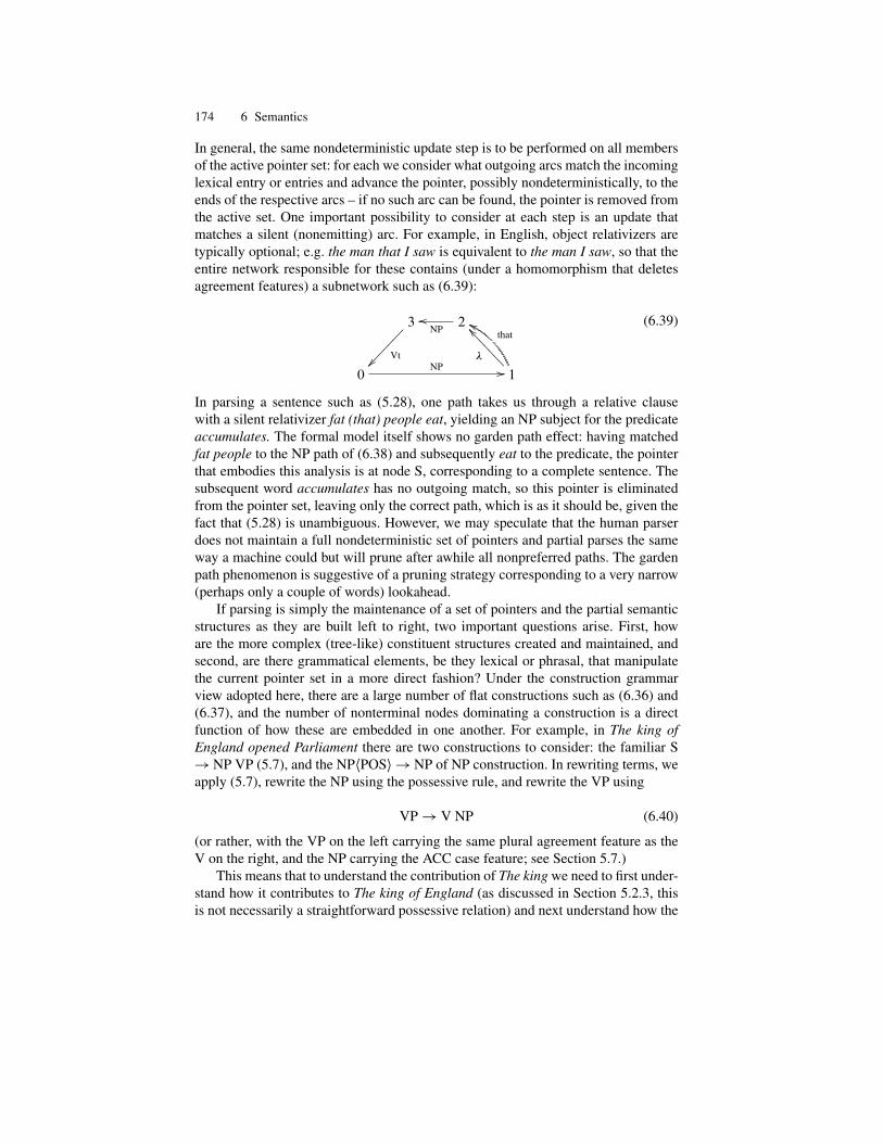
174 6 Semantics

In general, the same nondeterministic update step is to be performed on all membersof the active pointer set: for each we consider what outgoing arcs match the incominglexical entry or entries and advance the pointer, possibly nondeterministically, to theends of the respective arcs – if no such arc can be found, the pointer is removed fromthe active set. One important possibility to consider at each step is an update thatmatches a silent (nonemitting) arc. For example, in English, object relativizers aretypically optional; e.g. the man that I saw is equivalent to the man I saw, so that theentire network responsible for these contains (under a homomorphism that deletesagreement features) a subnetwork such as (6.39):

3

Vt������

���

2NPoo

0NP // 1

�

^^=======

thatgg (6.39)

In parsing a sentence such as (5.28), one path takes us through a relative clausewith a silent relativizer fat (that) people eat, yielding an NP subject for the predicateaccumulates. The formal model itself shows no garden path effect: having matchedfat people to the NP path of (6.38) and subsequently eat to the predicate, the pointerthat embodies this analysis is at node S, corresponding to a complete sentence. Thesubsequent word accumulates has no outgoing match, so this pointer is eliminatedfrom the pointer set, leaving only the correct path, which is as it should be, given thefact that (5.28) is unambiguous. However, we may speculate that the human parserdoes not maintain a full nondeterministic set of pointers and partial parses the sameway a machine could but will prune after awhile all nonpreferred paths. The gardenpath phenomenon is suggestive of a pruning strategy corresponding to a very narrow(perhaps only a couple of words) lookahead.

If parsing is simply the maintenance of a set of pointers and the partial semanticstructures as they are built left to right, two important questions arise. First, howare the more complex (tree-like) constituent structures created and maintained, andsecond, are there grammatical elements, be they lexical or phrasal, that manipulatethe current pointer set in a more direct fashion? Under the construction grammarview adopted here, there are a large number of flat constructions such as (6.36) and(6.37), and the number of nonterminal nodes dominating a construction is a directfunction of how these are embedded in one another. For example, in The king ofEngland opened Parliament there are two constructions to consider: the familiar S! NP VP (5.7), and the NPhPOSi ! NP of NP construction. In rewriting terms, weapply (5.7), rewrite the NP using the possessive rule, and rewrite the VP using

VP ! V NP (6.40)

(or rather, with the VP on the left carrying the same plural agreement feature as theV on the right, and the NP carrying the ACC case feature; see Section 5.7.)

This means that to understand the contribution of The king we need to first under-stand how it contributes to The king of England (as discussed in Section 5.2.3, thisis not necessarily a straightforward possessive relation) and next understand how the

6.3 Grammatical semantics 175

whole NP contributes to the sentence (by binding the Agent valency of open). Alto-gether, the depth of the phrase structure tree corresponds exactly to the degree thatconstructions are recursively substituted in one another, and there seems to be noprincipled limitation on this. To the extent we see a limitation, it is on the number ofpointers k that can be maintained simultaneously in human memory. What the gar-den path phenomenon suggests is that this limit is at two. (Even k D 2 is somethingof a stretch: in reality, when the first parse dies out, what we need to do is to recallthe whole sentence from short-term auditory memory and restart the process – thesecond pointer is there to keep the mechanism from taking the path it took the firsttime by marking that particular analysis as dead).

In the strict left to right parsing model assumed here, each partial parse leads toa deterministic state, with different parsing alternatives typically corresponding todifferent states, though we leave open the possibility of pointer paths merging. Con-sider the initial sequence Who did which can be completed in many ways: by an insitu question particle what?; by an objectless clause Mary see?; by far more complexconstructions such as her parents think would be the best match for Mary?; or, if weare willing to treat question intonation as a boundary melody, simply by this melody(orthographically represented as ? in these examples). The last case corresponds tosluicing questions, typically uttered by a person different from the one who utteredthe lead sentence: A: John decided to buy an airplane. B: Who did? As there areat least two different senses of who to consider (one of which can be replaced bywhom in a stylistically marked variant of English, but the other cannot) and thereare at least two different senses of did, we can entertain four different paths throughthe state machine. At this state of the parse, the string Who did has a nondetermin-istic analysis (pointer set) composed of these four possibilities: depending on thecontinuation, only one will be an initial segment of the complete parse.

One peculiarity of the state machines arising in natural language syntax is that atany given stage of the left to right parse, at least one of the pointers in the currentlyactive set is close to a final state. Consider the initial sequence After a good. A com-plete continuation could be boy does his homework, he may play – this requires sevenwords. However, a much shorter continuation, with meal, leave, is also available: wetake advantage of the fact that in English an intransitive verb alone is sufficient toform an imperative sentence (a form of the lexicality constraint discussed in Sec-tion 5.1.3) and also of the observation (see Erdelyi-Szabo et al. 2007) that nounssuch as storm, meal, etc., supply temporal coordinates (typecasting meal to S is asilent move). Since the construction (6.36) involves two sentences, in the homeworkcontinuation a pointer different from that used in the meal case will survive, but thesituation is analogous to chess, where we may consider deeply embedded structuresof gambits and counter-gambits, but a fast way out, by one player resigning, is alwaysavailable.

How big is the state machine? In Corollary 4.4.1, we demonstrated that vocabu-lary size is infinite, but in Section 5.1.1 we argued that the set of strict (sub)categoriesC is finite – in Section 5.2.2 we estimated, rather generously, jC j to be below7:7 � 1023. A more realistic estimate is 106, subdirectly composed of some 103 lex-ical classes with some 103 inflectional possibilities. By the preceding observation,

176 6 Semantics

any active pointer set has at least one member that is within a few (say, five) steps ofbecoming final. As there are at most jC j5 � 1030 five-step continuations, and thereis a pointer in any active set (with at most k members) that leads to a final state bysuch a continuation, there can be at most k � 1030 states, given that those states thatcan never be reached by any member of an active set can obviously be pruned. Again,the estimate is rather generous: in reality, much shorter continuations suffice and nomore than 1012 states are expected, even if we permit k > 2. While this number maystill look too large, what really matters is not the raw number of states and transitionsbut rather the manner in which these are organized – the overall complexity of thesystem (see Chapter 7) is considerably smaller than these numbers may suggest.

Lexicality, taken in a broad sense, amounts to the statement ‘if it can be doneby a phrase, it can be done by a single word’. So when we ask the general questionwhether phrases can manipulate the active pointer set in a manner more direct thanthe continuation tracking discussed so far, what we would really like to see are lexicalentries capable of such manipulation. A striking example is provided by coordinat-ing conjunctions, in particular and. Consider the initial segment Mary wanted and.This has two major continuations of interest here: obtained records and Bill obtainedrecords. Absent the rather characteristic intonation pattern (orthographically repre-sented as ;) of NCC, the preferred path is with constituent coordination: wanted andobtained become parallel verbs whose Agent valency is filled by Mary and whoseGoal valency is filled by records. However, when we see the next element, Bill, thispath is no longer available, and it is Mary wanted that needs to be made parallel withBill . This can only be done if and has the power to introduce new active pointersnondeterministically at each previously traversed state. The continuation Bill is thenfree to take the first of these. One argument in favor of treating and in this fashion isthat it can occur in the initial position: And now, ladies and gentlemen,. . .

How are the semantics portions of signs to be combined? Since constructionssuch as (6.37) cannot be recognized until the formatives is to, as, is to that definethem are supplied, the relevant semantic function �.s1/=�.s2/ D �.s3/=�.s4/ can-not be fully invoked at the stage London is. To invoke it partially, �.London/=�.s2/ D

�.s3/=�.s4/ must already at this stage be maintained as one of the nondeterministicanalyses, only to discard it when the next word, foggy, arrives. Psychologically it maymake more sense to assume that processing is deferred at least until a complete con-stituent is collected, just as in the processing of predicate calculus formulas, whereinterpretation proceeds through well-formed subformulas, but we have no intentionhere of presenting a psychologically realistic parsing model (see Section 5.6); ourgoal is simply to build a formal account couched in parsing terms.

The real issue, then, is whether disjoint pieces must be kept in partial parses orwhether a single combined sign must be available at each turn. The problem is wellillustrated by the case of English transitives, which, according to most theories, arebuilt using the rules (5.7) and (6.40). In other words, the construction Vt NP itself isequivalent to an intransitive verb, and since its semantic representation can only bebuilt after the object is available, the whole construction cannot be interpreted earlier.To implement this view as a parsing strategy would require keeping track of The kingof England and opened, and once Parliament comes under scan, combine it first with

6.4 Further reading 177

opened and combine only the result with The king of England. In the proposal madehere, (6.35) makes the formalism strong enough to carry out the substitutions in anyorder, so that the Agent VBTO of AxGy open.x; y/ can bind The king of Englandwithout assuming the existence of a constituent The king of England opened. To theextent scope-taking does not follow the linear order, we may still want to invoke adelay mechanism such as Cooper storage (see Cooper 1975), but, given our obser-vations about the defeasability of quantifiers, much of the standard evidence in favorof such a mechanism needs significant reexamination.

6.4 Further reading

The Liar paradox goes back to the 4th century BCE. The solution adopted here is es-sentially that of Barwise and Etchemendy (1987), using the elementary formulationof Walker (2003) rather than the more technical ZFC�+ Anti-Foundation Axiom-based version (Aczel 1988) that is now standard. Other notable efforts at a solutioninclude three-valued logic (for a thorough discussion, see Visser 1989) and para-consistent logic (Priest 1979, Priest et al. 1989). Read (2002) and Restall (2007)reconstruct the work of the medieval logician Thomas Bradwardine, who reaches,by rather different means, the same conclusion, that (6.1) is not contradictory, it isfalse. Our desideratum (C), which amounts to some strong form of direct compo-sitionality, is somewhat controversial, see Janssen (1997) and Barker and Jacobson(2007).

For the interaction of language and number systems, see Hurford (1975) andWiese (2003). For propositional attitudes, see in particular Frege (1879), Quine(1956), Barwise and Perry (1983), or the short tutorial summary by Bauerle andCresswell (1989). Although our conclusions are diametrically opposed, our discus-sion is greatly indebted to Thomason’s (1980) summary of the prerequisites forTarski’s undefinability theorem. For an alternative view on the viability of quota-tional theories see des Rivieres and Levesque (1986). Another alternative treatmentof opacity, based on structured meanings, was developed in Cresswell (1985). SeeOjeda (2006a) for detailed argumentation why a nonintensional treatment is to bepreferred both on grounds of simplicity and grounds of adequacy.

With the Principle of Responsibility, our discussion departs somewhat from theMG tradition in that we make lexical semantics carry a great deal of the explanatoryburden. MG in general is silent on the meaning of lexical entries: aside from somemeaning postulates that tie the meaning of nonintensional verbs and nouns to theirintensionalized meanings, only a few function words are ever assigned translations,and attempts to push the basic techniques further (see in particular Dowty 1979)go only as far as purely logical meanings can be assigned. For nominals see Puste-jovsky (1995). The method of defining lexical entries in terms of their essential prop-erties goes back to Aristotle and is perhaps best articulated in contemporary termsby Wierzbicka and the NSM school. For a recent critique of this approach, fueledlargely by the ideas of Kripke (1972) already discussed here, see Riemer (2006). Al-though the use of generalized quantifiers is often viewed as characteristic of MG, the

178 6 Semantics

idea goes back to Leibniz and was stated in modern terms as early as in Mostowski(1957).

A good starting point for generics is Carlson and Pelletier (1995). That gener-ics admit exceptions and thus require a mechanism greatly different from that ofstandard quantification has long been noted (Jespersen 1924). For a summary evalu-ation and quick dismissal of nonmonotonic approaches to generics, see Pelletier andAsher (1997), and for a more sympathetic view, see Thomason (1997) in the samevolume. The standard treatment of exceptions is Moltmann (1995), who takes theexception domain to be subtracted from each element in the set of properties thatmake up a generalized quantifier (see also Lappin 1996). In our case, only essentialproperties are used, and the exception domain could be subtracted from them, but ourdiscussion here is also compatible with the view that those essential properties thatare contradicted by the exception get dropped out entirely. The possibility of usingparaconsistent logic has already been considered by Bauerle and Cresswell (1989);

Possibly we would need in addition a nonstandard propositional logic, per-haps e.g. the kind that Belnap (1977) thinks a computer should use whenreasoning from inconsistent information.

but they dismissed it promptly on the grounds that “it is hard to see how any approachof this kind can guarantee that we have enough impossible worlds”. We use Gins-berg’s (1986) system D, which combines paraconsistency with default reasoning.

The idea of eliminating bound variables from logic goes back to Schonfinkel(1924), but fuller development begins with Curry and Feys (1958) and Quine (1961).Suppes (1973) and Suppes and Macken (1978) credit the idea to Peirce; see alsoPurdy (1992) and Bottner (2001). For a summary of the main ideas from both thelinguistic and the mathematical perspectives, see Barker (2005), where both the stan-dard analyses with variables and the variable-free approach pioneered by Szabolcsi(1987), Jacobson (1999), and others are discussed. Another approach, doing awaywith variables in favor of arbitrary objects, is introduced in Fine (1985).

Karakas are discussed in Staal (1967) and Kiparsky (2002). The use of VBTOs(in particular, lambda-operators) to capture argument linking was suggested in lec-tures by Manfred Bierwisch (1988). For c-categorial grammars, we could not locateany specific reference, but the idea of using concatenated (direct product) categoriesis part of the folklore. Some of the ideas about pointer set maintenance go back tounpublished work of the author and Laszlo Kalman, in particular Kornai and Kalman(1985). The sluicing phenomenon was identified (and named) by Ross (1969); for arecent overview see Merchant (2001).

Historically, only the MG tradition of linguistic semantics has been presented ina fully formalized manner, but many of the ideas presented in this chapter have beenstated quite clearly, if informally, in studies such as Wierzbicka (1985), Langacker(1982, 1987, 1991), Fauconnier (1985), and Jackendoff (1972, 1983, 1990).

7

Complexity

Grammars are imperfect models of linguistic behavior. To the extent that we aremore interested in competence than in performance (see Section 3.1), this is ac-tually desirable, but more typically discrepancies between the predictions of themodel and the observables represent serious over- or undergeneration (see Sec-tion 2.2). There is, moreover, an important range of models and phenomena where itis not quite obvious which of the cases above obtain. Suppose the task is to pre-dict the rest of the series 2; 3; 5; : : :. A number of attractive hypotheses presentthemselves: the prime numbers, the Fibonacci numbers, square-free numbers, thesequence 2; 3; 5; 2; 3; 5; 2; 3; 5; : : :, and so on. The empirically minded reader mayobject that the situation will be greatly simplified if we obtain a few more data points,but this is quite often impossible: the set of actual human languages cannot be ex-tended at will.

Therefore, it would be desirable to have an external measure of simplicity, sothat we can select the best (most simple) hypothesis compatible with a given rangeof facts. Starting with Pan. ini, linguists tend to equate simplicity with shortness, andthey have devoted a great deal of energy to devising notational conventions that willmake the linguistically attractive rules and generalizations compactly expressible.The central idea is that such notational conventions get amortized over many rules,so in fact we can introduce them without seriously impacting the overall simplicityof the system.

In this chapter, we begin to develop such a theory of simplicity. In Section 7.1 weintroduce the basic notions of information and entropy, and in Section 7.2 we presentthe basic theory of Kolmogorov complexity originally put forth in Solomonoff(1964). Section 7.3 deals with the more general problem of inductive learning fromthe perspective of complexity.

7.1 Information

In the classical model of information theory (Shannon 1948), the message to be trans-mitted is completely devoid of internal structure: we are given a (finite or infinite) set

180 7 Complexity

A D fa1; a2; : : :g of elementary messages and a probability distribution P over A.More complex messages are formed by concatenating elementary messages, and it isassumed that this is a Bernoulli experiment, so that the choice of the next elementarymessage is independent of what went on before. To transmit one of the ai , we needto encode it as a bitstring C.ai /. We need to make sure that C is invertible and thatCC W AC ! f0; 1gC, defined by lifting C to be a (concatenation-preserving) homo-morphism, will also be invertible. This is trivially satisfied as long as no codeword isa prefix of another codeword (i.e. the code is prefix-free) since in that case we knowexactly where each codeword ends (and the next one begins) in the stream of bitstransmitted.1

Exercise 7.1 Construct a codeC such thatC is not prefix-free butCC is neverthelessinvertible.An important subclass of prefix-free codes are fixed-length codes, where the lengthni of C.ai / is constant (usually a multiple of eight). However, in the cases that areof the greatest interest for the theory, the number of elementary messages is infinite,so no fixed-length code will do. Prefix-free variable-length binary codes will satisfythe following theorem.Theorem 7.1.1 Kraft inequality. In a prefix-free code, if ci are codewords of lengthni , X

i

2�ni � 1 (7.1)

Proof A prefix-free set of codewords can be depicted as a binary tree, where eachsequence of zeros and ones corresponds to a unique path from the root to a leaf node,zero (one) meaning turn left (right). For the tree with two nodes, (7.1) is triviallysatisfied (as equality). Since all prefix codes can be obtained by extending a leaf oneor both ways, the result follows by induction for finite codes and, by standard limitarguments, for infinite codes as well.Given a probability distribution P, Shannon-Fano codes are computed by an algo-rithm that constructs this tree top-down by dividing the total probability mass in twoparts recursively until each node has only one elementary message. Shannon-Fanocodes are of historical/theoretical interest only: in practical applications, the numberof elementary messages is finite, and the more efficient Huffman codes, where thetree is created from the bottom up starting with the least probable message, havereplaced Shannon-Fano codes entirely.Exercise 7.2 Specify the top-down algorithm in more detail using raw (cumulative)probabilities. Compare your algorithms with the actual Fano (Shannon) algorithms.Specify the bottom-up procedure, and compare it with the Huffman algorithm. Doany of these procedures fit the notion of a greedy algorithm?Now we introduce the quantity H.P / D �

Pi p log2 p, known as the entropy of

the distribution P . While the definition of H may at first blush look rather arbitrary,

1 Somewhat confusingly, codes enjoying the prefix-free property are also called prefix codes.

7.1 Information 181

it is, up to a constant multiplier (which can be absorbed in the base of the logarithmchosen) uniquely defined as the function that enjoys some simple and natural prop-erties we expect any reasonably numerical characterization of the intuitive notion ofinformation to have.Theorem 7.1.2 (Khinchin 1957) Uniqueness of entropy. We investigate nonnegative,continuous, symmetrical functions I.p1; p2; : : : ; pk/ defined for discrete probabilitydistributions P D fp1; p2; : : : ; pkg.

Ppi D 1/. (i) If P 0 is formed from P by

adding another outcome akC1 with probability pkC1 D 0, we require I.P / D I.P 0/.(ii) We require I to take the maximum value in the equiprobable case pi D 1=k. (iii)For P;Q independent we require I.PQ/ D I.P /C I.Q/ and in general we requireI.PQ/ D I.P /CI.QjP /: The only functions I satisfying the conditions above are�c

Ppi log.pi / D cH for arbitrary nonnegative constant c.

Proof Let us denote the maximum value I.Pk/ taken in the equiprobable case Pk D

f1=k; 1=k; : : : ; 1=kg by l.k/. By (i) we have l.k/ � l.kC 1/. By property (iii), tak-ing r independent distributions Pk , we have l.kr / D l.P r

k/ D l.Pkr / D rl.k/. Let-

ting k D ez and l.ex/ D B.x/, this functional equation becomes B.zr/ D rB.z/,which, by a well-known theorem of Cauchy, can only be satisfied by B.z/ D cz

for some constant c, so l.ez/ D cz, and thus l.k/ D c log.k/ (and by the mono-tone growth of l established earlier, c > 0). Turning to the nonequiprobable casegiven by rational probabilities pi D ni=n, we defineQ to contain n different events,divided into k groups of size ni , such that the conditional probability of an eventin the i th group is 1=ni if ai was observed in P and zero otherwise. This way,we can refer to the equiprobable case for which I is already known and computeI.QjP / D c

PkiD1 pi log.ni / D c

PkiD1 pi log.pi /Cc log.n/. In the joint distribu-

tion PQ, each event has the same probability 1=n, so that I.PQ/ D c log.n/. Givenour condition (iii), we established I.P / D �c

PkiD1 pi log.pi / for pi rational and

thus by continuity for any pi . ThatH indeed enjoys properties (i)–(iii) is easily seen:(i) is satisfied because we use the convention 0 log.0/ D 0 (justified by the limit prop-erties of x log.x/), (ii) follows by Jensen’s inequality, and finally (iii), and the moregeneral chain rule H.P1P2 : : : Pk/ D H.P1/CH.P2jP1/CH.P3jP1P2/C : : :C

H.PkjP1P2 : : : Pk�1/ follows by simply rearranging the terms in the definition.Discussion There are a range of other theorems that establish the uniqueness of H(see in particular Lieb and Yngvason 2003), but none of these go all the way towardestablishingH as the appropriate mathematical reconstruction of the intuitive notionof information. One issue is that entropy is meaningful only over a statistical ensem-ble: the information content of individual messages is still a function (negative log)of their probability. Many authors find this counterintuitive, arguing e.g. that There isa leopard in the garden provides the same amount of information as There is a dog inthe garden, namely the presence of an animal. Even if we grant the point that prob-abilities are important (e.g. a message about a surprising event such as winning thelottery is more informative than a message about a likely event such as not winningit), outside the games of chance domain it is not at all trivial to assign reasonablebackground estimates to probabilities. Here we take the view that this is inevitableinasmuch as information content depends on our expectations: the same message, He

182 7 Complexity

had steak for dinner, is more informative about a supposed vegetarian than about ameat-and-potatoes guy.Exercise 7.3� Obtain a sample of English and count the frequency of each character,including whitespace. What is the grapheme entropy of the sample? How much is theresult changed by using e.g. Perl or C program texts rather than ordinary (newspaper)text in the sample?Exercise 7.4� Write a program that parses English into syllables, and count eachsyllable type in a larger sample. What is the syllable entropy of the text?While it is easiest to consider phonemes, graphemes, syllables, and other finite setsof elementary messages, the definition of entropy is equally meaningful for infinitesets and in fact extends naturally to continuous distributions with density f .x/ bytaking H.f .x// D �

R1

�1f .x/ log2.f .x//dx. Here we will consider English as

being composed of words as elementary messages and estimate its word entropy. Thetask is made somewhat harder by the fact that words, being generated by productivemorphological processes such as compounding (see Chapter 4), form an infinite set.Although the probabilities of the, of, to, a, and, in, for, that, and other frequent wordscan be estimated quite reliably from counting them in samples (corpora) of mediumsize, say a few million words, it is clear that no finite sample will provide a reliableestimate for all the (infinitely many) words that we would need to cover.

Therefore we start with Zipf’s law (see Section 4.4), which states that the r thword in the corpus will have relative frequency proportional to 1=rB , where B , theZipf constant, is a fixed number slightly above 1. To establish the constant of pro-portionality Ck , recall Herdan’s law that a corpus of size N will have about N 1=B

different words. Let us denote the cumulative probability of the most frequent kwords by Pk and assume Zipf’s law holds in the tail, so that we have

1 � Pk D Ck

N 1=BXrDkC1

r�B� Ck

Z N 1=B

k

x�Bdx DCk

.1 � B/ŒN

1�BB � k1�B � (7.2)

For large N , the first bracketed term can be neglected, and therefore we obtainCk � .1 � Pk/.B � 1/kB�1. The first k words, for relatively small fixed k, al-ready cover a significant part of the corpus: for example, the standard list in Volume3 of (Knuth 1971) contains 31 words said to cover 36% of English text, the 130–150most frequent collected in Unix eign cover approximately 40% of newspaper text,and to reach 50% coverage we need less than 256 words. To estimate the entropy, wetake

H D �

kXrD1

pr log2.pr / �

N 1=BXrDkC1

pr log2.pr / (7.3)

The first sum, denoted Hk , can be reliably estimated from frequency counts and ofcourse can never exceed the maximum (equiprobable) value of log2.k/. The secondsum can be approximated by integrals:

7.1 Information 183

CkB

log.2/

Z N 1=B

k

log.x/x�Bdx �Ck log.Ck/

log.2/

Z N 1=B

k

x�Bdx (7.4)

The value at the upper limit can be neglected for large N , so we get the followingtheorem.Theorem 7.1.3 The word entropy H of a language with Zipf constant B is given by

H � Hk C1 � Pk

log.2/.B=.B � 1/ � log.B � 1/C log.k/ � log.1 � Pk// (7.5)

H256 can be estimated from medium or larger corpora to be about 3.9 bits. P256 isabout 0.52, and B for English is about 1.25, so the estimate yields 12.67 bits, quiteclose to the � 12 bits that can be directly estimated based on large corpora (over abillion words). In other languages, the critical parameters may take different values.For example, in Hungarian, it requires the first 4096 words to cover about 50% ofthe data, and the entropy contributed by H4096 is closer to 4.3 bits, so we obtainH � 15:41 bits. Equation (7.5) is not very sensitive to the choice of k but is verysensitive to B . Fortunately, on larger corpora, B is better separated from 1 than Zipforiginally thought. To quote Mandelbrot (1961b:196):

Zipf’s values for B are grossly underestimated, as compared with valuesobtained when the first few most frequent words are disregarded. As a result,Zipf finds that the observed values of B are close to 1 or even less than 1,while we find that the values of B are not less than 1.

As we shall see in the following theorem, for prefix codes the entropy appears as asharp lower bound on the expected code length: no code can provide better “on thewire” compression (smaller average number of bits). Our estimate therefore meansthat English words require about 12 bits on average to transmit or to store – thiscompares very favorably to using 7-bit ascii, which would require about 35 bits (thefrequency-weighted average word length in English is about five characters).Theorem 7.1.4 (Shannon 1948) Let ai be arbitrary messages with probability pi andencoding C.ai / D ci of length ni such that

Pi pi D 1 and the set of codewords is

prefix-free,

L.P / D

Xi

pini � H.P / (7.6)

with equality iff the codewords are all exactly of length log2.1=pi /.Proof

H.P / � L.p/ D

Xi

pi log2

2�ni

pi

D log2 eX

i

pi ln2�ni

pi

(7.7)

184 7 Complexity

The right-hand side can be bound from above using ln x � x � 1, and by the Kraftinequality we get

H.P / � L.p/ � log2 eX

i

pi .2�ni

pi

� 1/ � 0 (7.8)

When probabilities are very far from binary fractions, direct encoding may entailconsiderable loss compared with the entropy ideal. For example, if p1 D :9; p2 D :1,the entropy is 0.469 bits, while encoding the two cases as 0 vs. 1 would require a fullbit. In such cases, it may make sense to consider blocks of messages. For example,three Bernoulli trials would lead tp 111 with probability .729; 110, 101, or 011 withprobability .081; 001, 010, or 100 with probability .009; and 000 with probability.001. By using 0 for the most frequent case, 110, 100, and 101 for the next three, andfinally 11100, 11101, 11110, and 11111 for the remaining four, we can encode theaverage block of three messages in 1.598 bits, so the average elementary messagewill only require 1:598=3 D 0:533 bits.Exercise 7.5 Prove that no block coding scheme can go below the entropy limit butthat with sufficiently large block size the average code length can approximate theentropy within any " > 0.Exercise 7.6 Prove that a regular language is prefix-free iff it is accepted by a DFSAwith no transitions out of accepting states. Is a prefix-free language context-free iffit is accepted by a DPDA with the same restriction on its control?In real-life communication, prefix-free codes are less important than the foregoingtheorems would suggest, not because real channels are inherently noisy (the standarderror-correcting techniques would be just as applicable) but because of the peculiarnotion of synchrony that they assume. On the one hand, prefix-freeness eliminatesthe need for transmitting an explicit concatenation symbol, but on the other, it makesno provision for BEGIN or END symbols: the only way the channel can operate isby keeping the sender and the receiver in perfect synchrony. In Section 7.2 we willdiscuss a method, self-delimiting, that makes any set of codewords prefix-free.Exercise 7.7 Research the role of the ascii codes 0x02 (STX), 0x03 (ETX), and 0x16(SYN).Variable-length codes (typically, Huffman encoding) therefore tend to be utilizedonly as a subsidiary encoding, internal to some larger coding scheme that has theresources for synchronization. We will discuss an example, the G3 standard of faxtransmission, in Section 9.3.Exercise 7.8 Take the elementary messages to be integers i drawn from the geomet-rical distribution (pi D 1=2i ). We define a complex message as a sequence of nsuch integers, and assume that n itself is geometrically distributed. How many bitswill the average complex message require if you restrict yourself to prefix-free codes(no blocking)? With blocking, what is the optimal block size? What is the optimumaverage message length if the restriction on prefix-freeness is removed?

7.2 Kolmogorov complexity 185

Human language, when viewed as a sequence of phonemes, shows very strong ev-idence of phonotactic regularities (i.e. dependence between the elementary mes-sages). If we choose syllables as elementary, the dependence is weaker but stillconsiderable. If we use morphemes as our elementary concatenative units, the de-pendence is very strong, and if we use words, it is again weaker, but far from neg-ligible. Besides its uses in the study of coding and compression, the importance ofentropy comes from the fact that it enables us to quantify such dependencies. Forindependent variables, we have H.PQ/ D H.P / C H.Q/ (see condition (iii) inTheorem 7.1.2 above), so we define the mutual information between P and Q asH.P /CH.Q/ �H.PQ/. Mutual information will always be a nonnegative quan-tity, equal to zero iff the variables P and Q are independent. We also introduce hereinformation gain, also known as relative entropy and Kullback-Leibler (KL) di-vergence, as X

i

pi log2.pi=qi / D �H.P / �

Xi

pi log2.qi / (7.9)

where the last term, denoted H.P;Q/, is known as the cross entropy of P andQ. The importance of K-L divergence and cross entropy lies in the fact that thesequantities are minimal iff P D Q, and thus methods that minimize them can be usedto fit distributions.

All forms of communication that are parasitic on spoken language, such as writ-ing, or exercise the same fundamental cognitive capabilities, such as sign language,are strongly non-Bernoullian. Other significant sources of messages, such as musicor pictures, also tend to exhibit a high degree of temporal/spatial redundancy, as weshall discuss in Chapters 8 and 9.

7.2 Kolmogorov complexity

The model described above is well suited only for the transmission of elementarymessages that are truly independent of one another. If this assumption fails, redun-dancy between successive symbols can be squeezed out to obtain further compres-sion. Consider, for example, the sequence of bits 010100101011... that is obtainedby taking the fractional part of n

p2 and emitting 1 if greater than .5 and 0 other-

wise. It follows from Weyl’s theorem of equidistribution that P(0) = P(1) = .5. Theentropy will be exactly 1 bit, suggesting that the best we could do was to transmitthe sequence bit by bit: transmitting the first n elementary messages would requiren bits. But this is clearly not the best that we can do: to generate the message at theother side of the channel requires only the transmission of the basic algorithm, whichtakes a constant number of bits, plus the fact that it needs to be run n times, whichtakes log2 n bits.

We have not, of course, transcended the Shannon limit but simply put in sharprelief that entropy limits compressibility relative to a particular method of transmis-sion, namely prefix-free codes. The faster method of transmitting 010100101011...

186 7 Complexity

requires a great deal of shared knowledge between sender and recipient: they bothneed to know what p is and how you compute it, and they need to agree on for-loops, if-statements, a compare operator, and so on. Kolmogorov complexity isbased on the idea that all this shared background boils down to the knowledge re-quired to program Turing machines in general or just one particular (universal) Tur-ing machine.

Turing’s original machines were largely hardwired, with what we would nowa-days call the program burned into the finite state control (firmware) of the machine.For our purposes, it will be more convenient to think of Turing machines as universalmachines that can be programmed by finite binary strings. For convenience, we willretain the requirement of prefix-freeness as it applies to such programs. We say thata partial recursive function F.p; x/ is self-delimiting if for any prefix q of the pro-gram p; F.q; x/ is undefined. This way, a sequence of programs can be transmittedas a concatenation of program strings. The second variable of F , which we think ofas the input to the machine programmed by p, is a string of natural numbers or rathera single (e.g. Godel) number that is used to encode strings of natural numbers.Definition 7.2.1 The conditional complexity CF .xjy/ of x given y is the length ofthe smallest program p such that x D F.p; y/, or 1 if no such program exists.To remove the conditional aspects of the definition, we will need two steps, one en-tirely trivial, substituting y D 0, and one very much in need of justification, replacingall F s by a single universal Turing machine U .Definition 7.2.2 The complexity CF .x/ of x relative to F is the length of the small-est program p such that x D F.p; �/, or 1 if no such program exists.Theorem 7.2.1 (Solomonoff 1960, Kolmogorov 1965) There is a partially recursivefunction U.p; y/ such that for any partially recursive F.p; y/ there exists a constantcF satisfying

CU .xjy/ � CF .xjy/C cF (7.10)

Proof We construct U by means of a universal Turing machine V.a; p; x/ that canbe programmed by the appropriate choice of a to emulate any F.p; x/. To force theprefix-free property, for any string d D d1d2 : : : dn, we form d0 D d10d20 : : : 0dn1

by inserting 0s as concatenation markers and 1 as an end marker. Since any binarystring p can be uniquely decomposed as an initial segment a0 and a trailer b, we candefine U.p; x/ by V.a; b; x/. In particular, for F.p; x/ there is some f such that forall p; x F.p; x/ D V.f; p; x/. In case x can be computed from y by some shortestprogram p running on F , we have U.f 0p; y/ D V.f; p; y/ D F.p; y/ D x, so thatCU .x; y/ � 2jf j C CF .xjy/.Discussion There are many ways to enumerate the partial recursive functions, andmany choices of V (and therefore U ) could be made. What Theorem 7.2.2 means isthat the choice between any two will only affect CU .xjy/ up to an additive constant,and thus we can suppress U and write simply C.xjy/, keeping in mind that it isdefined only up to a O.1/ term. In particular, relative to the Turing machine T that

7.2 Kolmogorov complexity 187

prints its input on its output and halts, we see CT .x/ � l.x/C cT for some constantcT that is independent of the bitstring x (or its length l.x/).

The claim is often made (see e.g. Chaitin 1982) that C.x/measures the complex-ity of an individual object x, as opposed to entropy, which very much presumed thatthe objects of study are drawn from a probability distribution. However, this claim issomewhat misleading since the focus of the theory is really the asymptotic complex-ity of a sequence of objects, such as initial substrings of some infinite string, wheretheO.1/ term can be really and truly neglected. For a single object, one could alwaysfind a U that will make CU .x/ zero, just as if our only interest was in compressinga single file, we could compress it down to 1 bit, with an uncompress function thatprints out the object in question if the bit was set and does nothing otherwise.

To take advantage of asymptotic methods, one typically needs to endow famil-iar unordered objects with some kind of order. For example, formal languages areinherently unordered, but it is no great stretch to order †� (or any L � †�) lexico-graphically. Once this is done, we can talk about the nth string and replace sets bytheir characteristic function written as a (possibly infinite) bitstring whose nth bit is 1or 0, depending on whether the nth string yn enjoyed some property or not. In orderto discuss regular languages, we need to capture the structure of the state machine inbitstrings. Given some language L � †� and any string x, we define � D �1�2 : : :

to be 1 on the nth bit �n iff the string xyn is inL – the first n bits of �will be denotedby �:n. Clearly, two strings x and x0 have the same � iff they are right congruent, sothat different � correspond to different states in the DFSM. For L regular, the first nbits of any � can be transmitted by transmitting the DFSA in O(1) bits, transmittingthe state (out of finitely many) to which the � in question corresponds (again O(1)bits), and transmitting the value of n, which requires no more than log2.n/ bits.Theorem 7.2.2 (Li and Vitanyi 1995) L � †� is regular iff there exists a constantcL depending on L but not on n such that 8x 2 †� C.�:n/ � log2.n/C cL.Discussion We have already seen the only if part – the converse depends on a lemma(for a proof, see Li and Vitanyi 1997, Claim 6.8.1) that for any constant cL there willbe only finitely many infinitely long bitstrings that have no more than log2.n/C cL

asymptotic complexity – once this is demonstrated, the rest follows by the usualconstruction of FSAs from right congruence classes.

Suppose our goal is to transmit bitstrings over a channel that transmits 0s and 1sin an error-free (noiseless) manner. Unless we have some out-of-band method ofindicating where the transmission of a given bitstring begins and ends, we need todevote extra bits to the boundary information. An inefficient but simple method isto prefix each string x by its own length l.x/. For this to work, we need to encodel.x/ in a manner that makes it recoverable from the code. This can be accomplishede.g. by giving it as a string of 1s (base one) and using 0 as the end marker – thisis called the self-delimiting code S of x. For example, S.001/ D 1110001. In thisencoding, l.S.x// D 2l.x/ C 1. Not only is S prefix-free, but the codeword and afollowing string y can be unambiguously reconstructed from any S.x/y by countingthe number of 1s with which it begins and slicing off as many bits following thefirst 0 as there were 1s preceding it. We can use this property of S to create a more

188 7 Complexity

efficient code D.x/, where the payload x is suffixed not to the base one encodingof the length but rather to S.l.x//, where l.x/ is given in base two rather than baseone; for example, D.001/ D S.11/001 D 11011001. While this particular examplecomes out longer, in general

l.D.x// D l.S.dlog2 l.x/e//C l.x/ � 2 log2 l.x/C l.x/C c (7.11)

i.e. the overhead of the transmission is now only 2 log2 l plus some small constant.People (mathematicians) have relatively clear intuitions about the randomness

of everyday (resp. mathematical) objects – certainly we feel that *furiously sleepideas green colorless is much more random than colorless green ideas sleep furi-ously, which at least has largely predictable ordering at the part of speech level. Ifthe sender and the recipient share this knowledge, e.g. because they are both speakersof English, it may be possible to transmit the second sentence (but not necessarilythe first) in fewer bits than it would take to transmit a random string of words. Kol-mogorov complexity offers a way to replace intuitions about randomness by rigorousdefinitions, but this comes at a price. As we have emphasized repeatedly, C.x/ is de-fined only up to an additive constant. One may think that by fixing a small ‘reference’universal Turing machine U this fudge factor could be removed, but this is not quiteso: for any fixed U , the function CU .x/ is uncomputable.Theorem 7.2.3 (Kolmogorov 1965) C.x/ is uncomputable.Proof Suppose indirectly that C.x/ W f0; 1g� ! N is computed by some TM: itis then possible to program another TM that outputs, for each n 2 N, some stringxn that has C.xn/ > n. Let the length of the program emulating this TM on theuniversal machine we chose be p: this means that C.xn/ � log2.n/ C p since wefound a program of total length log2.n/C p that outputs xn. Since p is fixed but theprogram by definition outputs an xn with C.xn/ > n, we have a contradiction for nsufficiently large, e.g. for n D 2p.p > 2/.

While Kolmogorov complexity oscillates widely and uncomputably, on the wholeC.x/ is well-approximated by l.x/. We have already seen that C.x/ < l.x/CO.1/,and for any constant k, only a small fraction of the bitstrings of length l can haveC.x/ � l � k. More precisely, as there are at most 2l�kC1 � 1 programs of length� l �k, these can encode at most 2l�kC1 �1 of the 2l bitstrings of length l , so theremust be at least one string xl for every l that is truly incompressible (has C.x/ D l),at least half of the strings of length l have C.x/ � l � 1, at least three-quarters haveC.x/ � l � 2, and in general at least 1 � 2�k have C.x/ � l � k.

To put this in perspective, in Section 7.1 we estimated the word entropy of En-glish to be around 12–13 bits. The readers who worked on Exercise 5.8 will knowthat in journalistic prose the median sentence length is above 15 words, so for morethan half of the sentences the simple encoding scheme would require over 180 bits.Were these typical among the bitstrings of length 180, only 2�30 (about one in abillion) could be compressed down to 150 bits or less. As we shall see in Chapter 8,sentences can be compressed considerably better.

7.3 Learning 189

Another way to show that only a few strings can have low Kolmogorov complex-ity is by reference to the Kraft nequality (Theorem 7.1.1) if we encode each stringwith its shortest generating program relative to some fixed string y. To make sure thisis a prefix-free code, we use K.xjy/; defined as the shortest self-delimiting programon some universal TM and called the prefix complexity instead of C.xjy/, whichwas defined as the shortest program, not necessarily self-delimiting. With the prefixnotion of Kolmogorov complexity, which differs from our previous notion at mostby 2 log2 C.xjy/, we have X

x2f0;1g�

2�K.xjy/� 1 (7.12)

The most important case is of course y D �. Here the Kraft inequality means that thenumbers 2�K.x/ sum to less than 1. Therefore, we can turn them into a probabilitymeasure either by adding an unknown event that has probability 1�

Px2f0;1g� 2�K.x/

or we can normalize by multiplying all values by a constant. Using this latter method,we define the universal probability distribution by taking the probability of a stringx to be 2�K.x/ (times some constant). Solomonoff (1964) arrived at this notion byconsidering the idea of programming a TM by a random sequence of bits. If theshortest program that leads to x has n bits, the probability of arriving at x by arandomly selected program is roughly 2�n since longer programs can contribute verylittle to this value.

The standard geometrical probability distribution over bitstrings with param-eter r > 1 simply assigns probability .1 � 1=r/.1=2r/l to any string of length l– in particular, the probability of the empty string � will be 1 � 1=r . This corre-sponds to an experiment in which 0s and 1s are chosen by tossing a fair coin, andat each step the experiment is continued with probability 1=r . Transmitting a ran-dom (incompressible) string x of length l actually requires more than l bits since wealso need to transmit the information that the transmission has ended. We can use(7.11) as an upper bound on the length of the full transmission, which would yield.1=2/lC2 log2.l/Cc for a string of length l . For each fixed r; when l is large enough,the universal distribution generally assigns smaller probability to a string than thegeometrical distribution would – the remaining probability mass is spent on the fewstrings that have low complexity.

7.3 Learning

Returning to our original example of predicting the next term of the series 2; 3; 5; : : :,we can see that to make this more precise we need to make a number of choices. First,what is the domain and the range of the function to be learned? Can the next termbe �? In mathematical linguistics, our primary interest will be with strings, but thisis not a significant limitation since strings can encode more complex data structuressuch as k-strings (see Section 3.3), parse trees (see Section 5.1), or even grammars(see below). A considerably harder issue is brought up by weighted (probabilistic)

190 7 Complexity

structures since it is not at all obvious that even a single real number, say the fre-quency of some feature of interest, can be learned.

Second, we need to specify the hypothesis space that delimits the choice of so-lutions. In the sequence learning and the closely related sequence prediction tasks, ifwe know that the only hypotheses worth considering are quadratic polynomials, theanswer is already given by knowing the value of the function at three points. If, onthe other hand, arbitrary degree polynomials or all computable functions are accept-able answers, no finite amount of data will uniquely identify one. In mathematicallinguistics, the main issue is to identify a grammar that can generate a given data set,and this, as we shall see, is so hard that it is worth considering simplified versions ofthe problem.

Third, we must specify the method of providing examples to the learning algo-rithm. For example, if the target to be learned is some formal language, it makes abig difference whether it gets presented to the algorithm in a fixed (e.g. lexicograph-ical) order, completely randomly, or perhaps following some prescribed probabilitydistribution. In the first case, we can be certain after a while that an example notencountered so far will never be encountered later (because we are past it in thelexicographical ordering); the two other methods of providing data have no suchclosed-world assumption.

Fourth, we need to have some criteria for success. We will consider two mainparadigms: identification in the limit (Gold 1967) and probable approximate correct-ness (Valiant 1984). By an algorithm capable of identification in the limit (iitl), wemean an algorithm that will produce a hypothesis in each step such that after somenumber of steps it will always produce the same hypothesis, and it is the correct one.If the algorithm can signal that it converged, we are speaking of finite identification –this is obviously a stronger criterion than iitl. By a probably approximately correct(pac) learning algorithm we mean one that is capable of approximating a family ofdistributions to an arbitrary degree with the desired (high) probability. But beforeturning to these, we need to capture the idea that the more complex (in the limitingcase, entirely random) the material, the harder it is to learn.

7.3.1 Minimum description length

The mathematical theory of learning, or inductive inference, is very rich, thoughby no means mature. Depending on how we specify a problem in the four dimen-sions above, a broad variety of results can be obtained. In applying the ideas of Kol-mogorov complexity to natural language phenomena, we are faced with two techni-cal problems. First, the languages of greatest interest in mathematical linguistics arenoncounting, both in the informal sense of being free of arithmetic aspects and in theprecise sense given by the noncounting property (5.29). In spite of the impressivesize of the state space (estimated at 1012 in Section 6.3.2), counter-free automata aremathematically simpler than the full FSA class, while Theorem 7.2.2 characterizesthe latter as having, for all x 2 †�, a constant cL conditional prefix complexityK.�:njn/ (or, what is the same, log2.n/ C cL Kolmogorov complexity). Since thewhole machinery of Kolmogorov complexity is defined only up to a constant (the

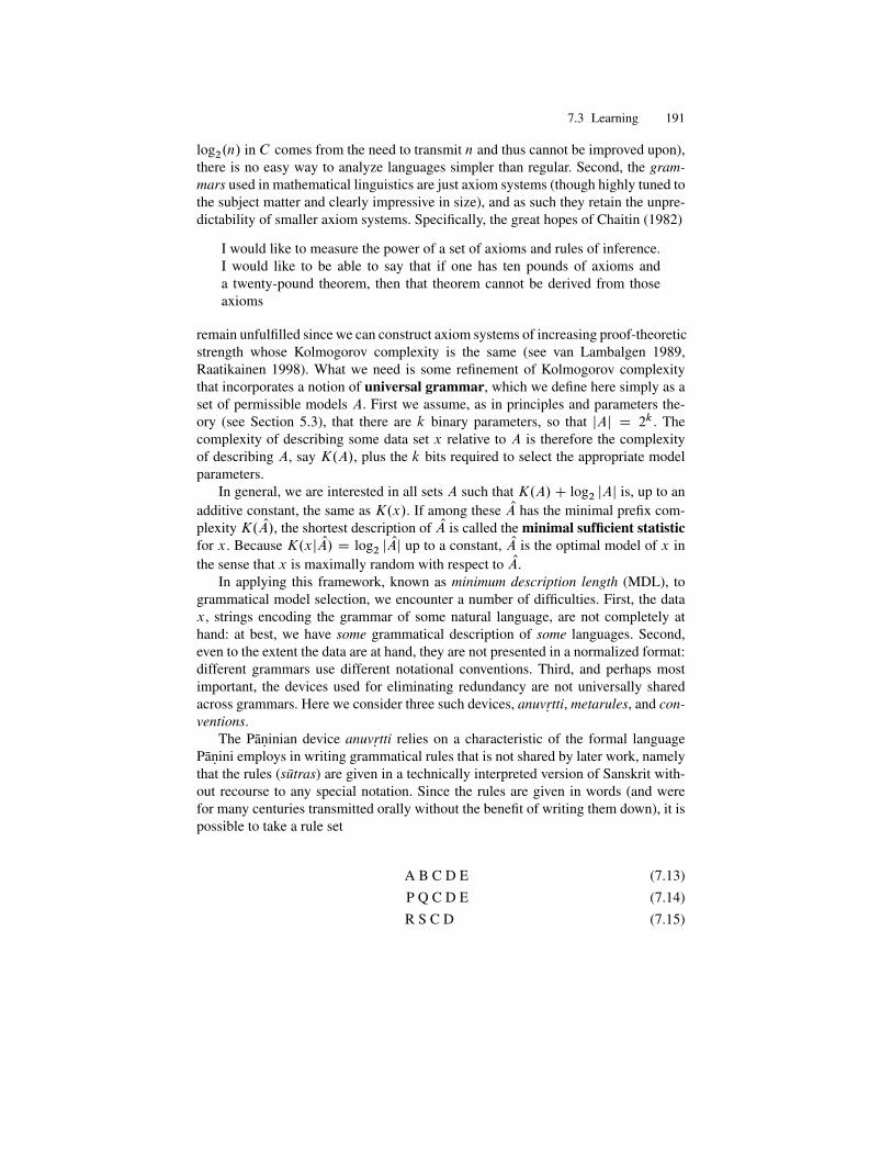
7.3 Learning 191

log2.n/ in C comes from the need to transmit n and thus cannot be improved upon),there is no easy way to analyze languages simpler than regular. Second, the gram-mars used in mathematical linguistics are just axiom systems (though highly tuned tothe subject matter and clearly impressive in size), and as such they retain the unpre-dictability of smaller axiom systems. Specifically, the great hopes of Chaitin (1982)

I would like to measure the power of a set of axioms and rules of inference.I would like to be able to say that if one has ten pounds of axioms anda twenty-pound theorem, then that theorem cannot be derived from thoseaxioms

remain unfulfilled since we can construct axiom systems of increasing proof-theoreticstrength whose Kolmogorov complexity is the same (see van Lambalgen 1989,Raatikainen 1998). What we need is some refinement of Kolmogorov complexitythat incorporates a notion of universal grammar, which we define here simply as aset of permissible models A. First we assume, as in principles and parameters the-ory (see Section 5.3), that there are k binary parameters, so that jAj D 2k . Thecomplexity of describing some data set x relative to A is therefore the complexityof describing A, say K.A/, plus the k bits required to select the appropriate modelparameters.

In general, we are interested in all sets A such that K.A/C log2 jAj is, up to anadditive constant, the same as K.x/. If among these OA has the minimal prefix com-plexity K. OA/, the shortest description of OA is called the minimal sufficient statisticfor x. Because K.xj OA/ D log2 j OAj up to a constant, OA is the optimal model of x inthe sense that x is maximally random with respect to OA.

In applying this framework, known as minimum description length (MDL), togrammatical model selection, we encounter a number of difficulties. First, the datax, strings encoding the grammar of some natural language, are not completely athand: at best, we have some grammatical description of some languages. Second,even to the extent the data are at hand, they are not presented in a normalized format:different grammars use different notational conventions. Third, and perhaps mostimportant, the devices used for eliminating redundancy are not universally sharedacross grammars. Here we consider three such devices, anuvr. tti, metarules, and con-ventions.

The Pan. inian device anuvr. tti relies on a characteristic of the formal languagePan. ini employs in writing grammatical rules that is not shared by later work, namelythat the rules (sutras) are given in a technically interpreted version of Sanskrit with-out recourse to any special notation. Since the rules are given in words (and werefor many centuries transmitted orally without the benefit of writing them down), it ispossible to take a rule set

A B C D E (7.13)P Q C D E (7.14)R S C D (7.15)

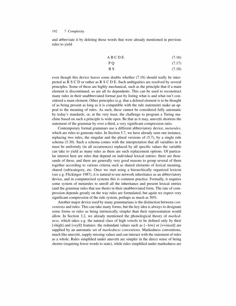
192 7 Complexity

and abbreviate it by deleting those words that were already mentioned in previousrules to yield

A B C D E (7.16)P Q (7.17)R S (7.18)

even though this device leaves some doubts whether (7.18) should really be inter-preted as R S C D or rather as R S C D E. Such ambiguities are resolved by severalprinciples. Some of these are highly mechanical, such as the principle that if a mainelement is discontinued, so are all its dependents. This can be used to reconstructmany rules in their unabbreviated format just by listing what is and what isn’t con-sidered a main element. Other principles (e.g. that a deleted element is to be thoughtof as being present as long as it is compatible with the rule statement) make an ap-peal to the meaning of rules. As such, these cannot be considered fully automaticby today’s standards, or, at the very least, the challenge to program a Turing ma-chine based on such a principle is wide open. Be that as it may, anuvr.tti shortens thestatement of the grammar by over a third, a very significant compression ratio.

Contemporary formal grammars use a different abbreviatory device, metarules,which are rules to generate rules. In Section 5.7, we have already seen one instance,replacing two rules, the singular and the plural versions of (5.7), by a single ruleschema (5.30). Such a schema comes with the interpretation that all variables in itmust be uniformly (in all occurrences) replaced by all specific values the variablecan take to yield as many rules as there are such replacement options. Of particu-lar interest here are rules that depend on individual lexical entries: there are thou-sands of these, and there are generally very good reasons to group several of themtogether according to various criteria such as shared elements of lexical meaning,shared (sub)category, etc. Once we start using a hierarchically organized lexicon(see e.g. Flickinger 1987), it is natural to use network inheritance as an abbreviatorydevice, and in computerized systems this is common practice. Formally, it requiressome system of metarules to unroll all the inheritance and present lexical entries(and the grammar rules that use them) in their unabbreviated form. The rate of com-pression depends greatly on the way rules are formulated, but again we expect verysignificant compression of the rule system, perhaps as much as 50%.

Another major device used by many grammarians is the distinction between con-ventions and rules. This can take many forms, but the key idea is always to designatesome forms or rules as being intrinsically simpler than their representation wouldallow. In Section 3.2, we already mentioned the phonological theory of marked-ness, which takes e.g. the natural class of high vowels to be defined only by their[+high] and [+syll] features: the redundant values such as [�low] or [+voiced] aresupplied by an automatic set of markedness conventions. Markedness conventions,much like anuvr.tti, supply missing values and can interact with the statement of rulesas a whole. Rules simplified under anuvr.tti are simpler in the direct sense of beingshorter (requiring fewer words to state), while rules simplified under markedness are

7.3 Learning 193

just regarded as being shorter, inasmuch as we explicitly define a simplicity measurethat only counts marked values. For example, context-sensitive voice assimilation inobstruent clusters is common, and a rule like

ŒCobst� ! Œ˛voice�=�

Cobst˛voice

�(7.19)

which requires cluster members to assimilate to their right neighbor in voicing, isregarded as intrinsically simple. However, since a rule like

ŒCsyll� ! Œ˛high�=�

Cobst˛voice

�(7.20)

is unlikely to crop up in the phonology of any language, we make sure that the sim-plicity measure penalizes it, e.g. for assimilation of values across features. Generally,a complicated simplicity measure is seen as a sign of weakness of the underlyingtheory. For example, if assimilation is viewed as spreading (see Section 3.3) of anautosegment, rules like (7.20) are precluded, and this obviates the need to patch mat-ters up by a post hoc simplicity measure. However, the working linguist is rarely ina position to anticipate future breakthroughs, so stipulation of simplicity remains apart of the descriptive apparatus.

To some extent, these problems can be circumvented by considering grammarspiecemeal rather than in their entirety. For example, stating the stress system of alanguage would require (i) finding its place in a typological system such as StressTyp(see Section 4.1.4) and (ii) describing the stress patterns relative to some slot inthe typology. Describing the ideally clean systems prescribed by the typology is anexpense that gets amortized over many languages, so the termK.A/ enters the overallcomplexity with a multiplier considerably lower than the term K.xjA/, which isspecific to the language. This is very much in line with traditional linguistic thinking,which values universal rules far more than parochial ones.

Unfortunately, decomposition of the grammar in this sense is not entirely unprob-lematic since one can often simplify the statement of one kind of rule, say the rulesof stress placement, at the expense of complicating some other part of the grammar,such as the rules of compounding. To apply the MDL framework would thereforerequire a problem statement that is uniform across various aspects of the system; forexample, by taking phonology, morphology, syntax, and semantics to be given byFSTs and assuming that universal grammar is a list of transducer templates that canbe filled in and made part of an intersective definition at no cost (or very little cost,given amortization over many languages).

One final issue to consider, not just for stress systems but for any situation wherethere are only a finite number of patterns, is whether generating the patterns by a rulesystem provides a solution that is actually superior to simply listing them. The issueis particularly acute in the light of theorems such asTheorem 7.3.1 (Tuza 1987) For every n there exists finite languages Ln containingn2 � n strings such that it requires at least O.n2= log.n// rules in a regular, context-free, or length-increasing (context sensitive) grammar to generate Ln.

194 7 Complexity

Discussion Since this is a worst case result, a possible objection is that the specificconstruction employed in Tuza (1987), namely languages based on n different termi-nals collected in a terminal alphabet † and Ln D fxyjx; y 2 †; x ¤ yg, is unlikelyto appear in natural language grammars. In phonology, rules of dissimilation thatforbid the occurrence of more than one token of some type are quite common (for abrief overview see Idsardi 2006), and there is no easy way to rule these out entirely.In syntactic rules, the phenomenon of lexicality (see Section 5.1.3) is quite perva-sive, so much so that for each preterminal (strict lexical subcategory) p we expect atleast one rule unique to p. With the size of the preterminal set estimated at 106 (seeSection 6.3.2), Theorem 7.3.1 limits the compression achievable by generation to afactor of

p. log.106// or to about 27% of the length of the raw pattern list (actually

less, since a rule will, in general, take more symbols to encode than a pattern would).Generative grammar, if viewed as a compression device which has the potential tosave three quarters of the space that would be required to list the patterns, is clearlya valuable tool in its basic (finite state, context free, or context sensitive) form, butthe other space-saving devices discussed here, anuvr.tti, metarules, and conventions,can enhance its compression power considerably.

7.3.2 Identification in the limit

To specify a learning problem in iitl terms, we need to specify the domain and therange of the functions to be learned, the hypothesis space, and the order in which datawill be presented to the learner. As an example, let us consider the issue of how in-fants acquire the phoneme inventory (see Section 3.1) of their language. The functionthey must identify is one that has at least acoustic input, utterances, and provides, foreach utterance, a string (or k-string), over a yet to be determined phonemic alphabet(or tier alphabets). We say the input consists at least in acoustic data because it isclear that the infant also has, almost all of the time, access to visual cues such as liprounding – we ignore this fact here but return to the matter in Section 8.3. We alsosimplify the problem statement by assuming the existence of automatic (no learn-ing or training required) low-level acoustical feature detectors that digest the rawacoustic signal into parallel streams of discrete feature sequences (see Section 8.3).

While this may look like drastic oversimplification, defining away a core partof the problem, in fact there is massive evidence from psycholinguistics that speechperception operates in terms of discrete units (a phenomenon known as categoricalperception, see Liberman 1957), that this mechanism is operative in infants even be-fore they learn to speak (Eimas et al. 1971), and that it leverages deep perceptualabilities that were acquired evolutionarily long before primates (for chinchilla per-ception of voicing and syllable structure see Kuhl et al. 1975). High sensitivity todistinctive features in the acoustical signal has been demonstrated for all the thirty orso features that act distinctively in the phonology of some languages. We defer theperceptual problem, how to create detectors for voicing or other features, to Chap-ters 8 and 9, and consider only the learning problem of finding the right phonemicalphabet based on the output of this exquisitely sensitive perceptual apparatus, givenin feature vectors. Instead of asking how acoustic waveforms (a class of R ! R

7.3 Learning 195

functions) get mapped onto (k-)strings, we ask how strings of feature vectors get somapped.

As for the hypothesis space, clearly the most desirable outcome would be to finda static mapping g that maps feature vectors to phonemes and obtain the sequence-to-sequence mapping by lifting g (applying it pointwise) to strings. Such a restrictionof the hypothesis space comes with a price: there are many string-to-string mappingsthat cannot be so obtained. For example, if the inputs are 0 and 1 (vectors of length 1)and the outputs are A and B , if f is defined as always A except when the previousthree inputs were 000 or 111, there isn’t a single g that can be lifted to f . A muchbroader, but still restrictive, hypothesis would be to assume that the solution is to beidentified with a (multitape) finite state (k-)transducer that outputs a phoneme (ork-string) based on the feature vector under scan on its input tapes and on its currentstate.

Finally, let us consider the order in which the data are presented to the learner.Even if the task is to find a function g that operates on individual vectors, it is notrealistic to assume (except, perhaps, for vowels that can be uttered in isolation) thatthe data will be presented pointwise – rather, the input is given in longer strings,syllables at the very least but more likely words or full sentences. In particular, stopconsonants will never occur in isolation, but their phonemic value must be learnedjust the same. Since there are only finitely many phonemes, a random presentationof words will sooner or later contain every one of them, and we do not particularlyneed to put any constraint on the presentation of the data other than those excludinga certain kind of child-directed speech (CDS, also called baby talk and motherese)that purposely avoids the sounds considered hard or stigmatized. Simplifying mat-ters somewhat, in modern-day Israel, Sefardic parents, whose phonemic inventorycontained guttural consonants, may not have passed these on to their children sincethe Ashkenazi variety of Modern Hebrew, which has higher prestige, lacks them. Anobvious restriction on data presentation, then, is to require that it be semicooperativein the sense that all relevant data (everything in the domain of the function to belearned) are eventually presented.

In reality, a great deal of language change can be attributed to imperfect learn-ing, but the Modern Hebrew case cited above is more the exception than the rule:phonemic inventories can be very stable and remain virtually unchanged over manygenerations and centuries. This is because the phoneme inventory can be iitl learnedupon any reasonable (semicooperative) presentation of the data. The chief learn-ing strategy appears to be selective forgetting. For example, Ntlaka’pamux [THP]has glottalized voiceless stop consonants that phonologically differ in place of ar-ticulation (uvular vs. velar), while English lacks this contrast and these consonantsaltogether. Learners of English who are 6–8 months oldrecognize the distinction justas well as Ntlaka’pamux infants of the same age, but by 11–12 months their abilityfades, while the Ntlaka’pamux infants of course retain it (Werker and Tees 1984). Inspite of the selective forgetting of those features that play no distinctive role in thelanguage, the full learning algorithm seems to involve a great deal of memorization.

The algorithms used by linguists to describe a new language, called discov-ery procedures, generally require more than semicooperation and assume full (two-

196 7 Complexity

sided) presentation of the data in the form of an informant who can provide negativeinformation (grammaticality judgments) as well, asserting if needed that a certainform hypothesized by the learner is not in the language. Both negative and very lowprobability positive examples help to accelerate the learning process, and this is whyin descriptive grammars we often find references to contrasts not easily exemplified.For example, in English, the difference between unvoiced s and voiced z is seen onlyin pairs like Aleutian/allusion, Confucian/confusion, mesher/measure, Asher/azure,and dilution/delusion, which are very unlikely to be heard by infants at an early age.That said, by age four, when children begin to show signs of acquiring morphology,the algorithm that yields the phonemic alphabet has clearly converged on the basis ofpositive data alone. How a phoneme like z gets created by the infant without a greatdeal of positive evidence is something of a mystery unless we presume a learningalgorithm that can only take a few options and must live with the resulting overgen-eration. If we find that voicing is distinctive in English, for which there is a greatdeal of positive evidence outside the s/z pair, and we find that s is present in the sys-tem, for which again there is overwhelming positive evidence, we must live with theconsequences and admit z in the system.

As our next example, let us consider iitl of finite automata. Given an alphabet T;a regular languageL � T �, and a text, defined here as a series of examples s1; s2; : : :drawn from L semicooperatively (each s 2 L sooner or later appears in the series)but possibly with repetitions, we are looking for an algorithm that produces at eachstep i a DFSA Ai that generates all the sj for 1 � j � i and converges to the DFSAA0 that generates L in the sense that there exists some k such that Ai D A0 fori > k.

Stated thus, the problem is not solvable. Let us first consider this for an importantalgorithm known as identification by enumeration. This is a lazy algorithm based onsome notion of complexity or a priori probability that can be used to linearly orderall possible hypotheses (DFSAs). At step i , it outputs the first (according to the pre-specified order) hypothesis that is still compatible with the data points s1; s2; : : : ; siseen so far. If the text is presented in an adversarial fashion, the algorithm can at nostage be certain that a string t not presented so far will not be presented later. What-ever complexity ordering the algorithm embodies, the DFSA U with one (accepting)state and loops for all symbols will come early in the enumeration in the sense thatwe need to entertain other (more complex) hypotheses as well, and the adversarycan pick any language L that is generated by one of these more complex DFSA V .Since the language T � generated by U is compatible with any finite amount of datapresented semicooperatively, a lazy algorithm will never have a reason to move awayfrom the hypothesis U and will never reach the correct hypothesis V .

An analogous situation can be found in the game of twenty questions: if there aremore than 220 animals (as there are), an answerer who knows the whole taxonomycan always win. The key idea is that the answerer need not settle on a particularanimal at the outset; it is enough that at any point there remain animals that fit thesequence of answers provided so far. Each question cuts the set of still availableanimals in two parts, and one of these sets will have more than 220�i members: theanswerer answers so as to select this set. After 20 questions, the answerer still has

7.3 Learning 197

more than one animal compatible with the questions asked so far and the questionerhas lost. In other words, since each question can secure at best one bit of information,and it requires more than 20 bits to code the full set of animals, the questioner cannotalways win (since a winning strategy would amount to a coding of the set in 20 bits)and an answerer can exploit the information deficit to make sure the questioner neverwins. Gold (1967) presents a similar strategy with adversarial (but semicooperative)data presentation to prove the following theorem.Theorem 7.3.2 (Gold 1967) No set of languages that contains all the finite languagesand at least one infinite language is iitl.Discussion Note that the theorem is sharp: the set of all finite languages is iitl,in fact the trivial algorithm that simply guesses the language to be the union ofthe strings presented so far will learn the correct language from any semicooper-ative text. A family of languages containing all finite languages and at least oneinfinite one is called superfinite, and since all the classical language families inthe Chomsky hierarchy are superfinite, the theorem is often taken to mean that iitlwith semicooperative data presentation is simply not the right model for grammarlearning. Yet there is no reason to assume that the set of languages permissibleby universal grammar will contain all finite languages; for example, the languagefa; aba; abba; abbba; abbbbag lacks the noncounting property (5.29) and is thusnot a (potential) natural language.

An indexed family of nonempty languages L1; L2; : : : satisfies Angluin’s Con-dition 1 iff there is an effective procedure that will create, for each i , a finite subsetTi of Li such that for all j , Lj 6� Li follows from Ti � Lj . The Ti is called atelltale for Li because once we know from semicooperative data presentation thatTi is part of the target language, no subsets Lj of Li need to be considered anymore.For such families, we have the following theorem.Theorem 7.3.3 (Angluin 1980) An indexed family of nonempty languages is iitl iffit satisfies Condition 1.For alphabets † with at least three letters, a classic construction of Thue (1906,reprinted in Nagell 1977) asserts the existence of an infinite word � D x1x2x3 : : :,which is square-free in the sense that no substring of it has the form ˛˛. For anythreshold k > 1, any regular set of subwords of � will be counter-free. Let us nowconsider the languageP0 D †� and the languagesPi obtained from†� by removingfrom †� the prefix x1; : : : xi of �. This is an indexed family of nonempty languagesthat are all regular (complement of a finite language) and noncounting (complementof a noncounting language) with threshold k for any k > 1. If this family is iitl, byTheorem 7.3.3 there is a finite telltale T0 such that for all j , Lj 6� †� must followfrom T0 � Lj . Since the conclusion is false but the premiss will be true for any Lj

with j greater than the longest string in T0, we have a contradiction that proves thefollowing theorem.Theorem 7.3.4 (Kracht 2007) For k > 1, the family of regular noncounting lan-guages over an alphabet † that has at least three elements is not iitl.Discussion To see that Theorem 7.3.3 is applicable, we need to assert that the lan-guages Pi are constructible. Thue’s original proof relies on the homomorphism h

198 7 Complexity

given by 0 ‘ 01201I 1 ‘ 020121I 2 ‘ 0212021 over the alphabet f0; 1; 2g andconstructs � as 0xh.x/h2.x/h3.x/ : : :, where x D 1201 (i.e. as the result of the infi-nite iteration of h from starting point 0). Since h increases the length of any string atleast by a factor of 5 (and at most by a factor of 7), it requires at most dlog.l/= log.5/eiterations to compute the prefix x1 : : : xl of � . Since the algorithm A.i; w/ that de-cides the membership of w in Pi needs only to test whether w is a prefix in �, it canrun in time and space linear in jwj.

Obviously, if A is an iitl learnable family, so is every B � A, and if C is notiitl learnable, neither will any D � C be iitl learnable. But this is not enough tocharacterize the iitl families since there are many incomparable iitl families, such asthe set of all finite languages vs. the set of all languages that can be generated byCSGs with a bounded number of rules (Shinohara 1990).

If we are prepared to relax the requirement of semicooperation (positive evidenceonly) and admit discovery procedures that rely on more data, there are several impor-tant results concerning regular languages and DFSAs. With a fully cooperative text(given in lexicographic order), Trakhtenbrot and Barzdin (1973) provided a polyno-mial algorithm that produces a DFSA consistent with all data (positive and negative)up to length n. If full cooperation is relaxed (positive and negative examples are pre-sented but not all up to a given length), the problem is NP-hard (Gold 1978). If co-operation is extended by the answerer (informant) providing not just yes/no answersbut also a full set of strings that reach every state of the automaton, the exact DFSAcan be learned in finite time (Angluin 1981). If grammar comparison is allowed inthe form of questions ‘Is this DFSA equivalent to the target?’, polynomial learning ofDFSAs is possible (Angluin 1987). It is equally possible to tighten the requirementof semicooperation by assuming a certain amount of downright misinformation orjust noise.

7.3.3 Probable approximate correctness

Assuming that each language learner is exposed to semicooperatively presented textfrom the older generations and identifies a grammar that can account for the text,there is still no guarantee that the learner’s grammar will be the exact equivalent ofthe grammars that were used in generating the text. In fact, languages can and dochange in aspects that go far beyond a superficial updating of vocabulary: wholegrammatical constructions fall into disuse and eventually disappear, paradigms sim-plify, new constructions and new paradigms enter the language at a surprising rate.Sometimes the process can be attributed to contaminated text, especially if there islarge-scale migration or change in ruling class, but even languages reasonably iso-lated from these effects change over time. To capture this phenomenon, we need toconsider some notion of approximate learning that involves some measure of simi-larity between what is learned and what should have been learned: the key idea ofValiant (1984) was to express approximation in probabilistic terms.

To specify a pac learning problem, we again need to specify the domain and therange of the functions to be learned. These are generally the characteristic functionsof some sets called concepts. We also need to specify the hypothesis space, generally

7.3 Learning 199

as a family H of concepts (sets) that are all subsets of the same universe calledthe sample space S . As the name suggests, S will be endowed with a fixed (butnot necessarily known) probability measure P that dictates both how data will bepresented to the learning algorithm and how the goodness of fit is to be measuredbetween the target concept C and a hypothesis C 0 proposed by the algorithm. Wesay that C 0 approximates C within " if P.C�C 0/ < " (here � is used to denotesymmetric set difference). As for our criterion of success, we say that an algorithmı; " pac-learns C if, after being presented with a sufficient number n of randomly(according to P ) chosen labeled examples, it produces, with probability > 1 � ı, aconcept C 0 that approximates C within ". Our chief interest is with algorithms thatare polynomial in n; 1=ı and 1=", and ideally we’d want algorithms that are robustunder change of the distribution P or even distribution-free (i.e. independent of P ).

As an example, let us again consider regular languages: the sample space is T �

endowed with a suitable (e.g. geometrical) probability distribution, a concept to belearned is some regular language C � T �, and a hypothesis produced by the al-gorithm is some DFSA c0, which generates the language C 0. Stated in pac terms,the problem is still hard. In particular, Kearns and Valiant (1989) demonstrate thata polynomial pac learner for all regular languages would also solve some problemsgenerally regarded as cryptographically hard. However, interleaving languages (themusical analog of k-strings; see Ross 1995) are pac learnable, and if membershipqueries are allowed, a polynomial pac discovery procedure for DFSAs exists (An-gluin 1987).

The Vapnik-Chervonenkis (VC) dimension of a space H of concepts is themaximum number of samples that can be labeled any way by members of H . Eachmember of H creates a binary decision (labeling) on S , and if a set of n is such thatall 2n labelings can be obtained by a suitable choice ofH , we say the set of points isshattered by H – the VC dimension of the hypothesis space is the cardinality of thelargest set that can be so shattered. Obviously, for a finite classH , the VC dimensionwill be � log2 jH j. The VC dimension of the hypothesis space is closely related topac learnability: the number of examples n needed for ı; " pac learning satisfies

�

�1

"log

1

ıCVC.H/

"

�� n � O

�1

"log

1

ıCVC.H/

"log

1

"

�(7.21)

While the two bounds are very close and the VC dimension of many classical learn-ing models is known, the error bounds computed from (7.21) are rather pessimisticboth because the results are distribution-free and because they are, as is common intheoretical computer science, worst-case results. In principle, many linguistic prob-lems could be recast as pac learning, but in a practical sense the algorithms that aremost important for the linguist owe little to the pac framework both because the VCbounds do not characterize the problem well and because linguistic pattern match-ing, to which we turn in Chapter 8, is generally concerned with n-way, rather than2-way, classification problems.

200 7 Complexity

7.4 Further reading

Although there is some interesting prehistory (Nyquist 1924, Hartley 1928), informa-tion theory really begins with Shannon (1948) – for a modern treatment, see MacKay(2003). The insufficiency of the classical quantitative theory of information has beenargued in Bar-Hillel (1964), whose goal was to replace it by a semantic theory ofinformation – the same goal is restated in Dretske (1981) and Devlin (1991). Devlin(2001) argues that the semantic theory that fits the bill is situation semantics; for ashort introduction, see Seligman and Moss (1997), and for a detailed exposition seeBarwise and Perry (1983).

Li and Vitanyi (1997) provide an encyclopedic treatment of Kolmogorov com-plexity. For a succinct presentation of the central ideas, see Gacs (2003) and for a dis-cussion of the relation of Kolmogorov complexity and learnability see Clark (1994).The MDL framework originates with Rissanen (1978). For a thorough discussionof anuvr.tti, invoking a full metagrammar of over a hundred principles, see Joshi andBhate (1984). The idea of using grammars to generate grammars goes back to Koster(1970). A significant fragment of English grammar, with heavy use of metarules, ispresented in Gazdar et al. (1985). The first major discussion of simplicity measuresin generative linguistics is Chomsky and Halle (1968 Ch. 9); for a comparison withthe earlier structuralist ideas, see Battistella (1996).

On the status of z, see McMillan (1977). The acquisition of phonology offers aparticularly rich storehouse of phenomena that support a universal grammar-basedview of language acquisition. For example, infants employ rules such as redupli-cation and final devoicing that the adult grammar of the language they learn mayentirely lack. However, the idea that the acquisition of phonology relies heavilyon hardwired UG has its detractors; see e.g. (Zamuner et al. 2005). The same canbe said for syntax, where the poverty of stimulus argument offered in Chomsky(1980), that certain facts about natural language could not be learned from expe-rience alone, though widely accepted, has significant detractors; see e.g. Pullum andScholz (2002).

The classic sources on iitl and pac learning remain Gold (1967) and Valiant(1984). For inductive inference in general, see Angluin and Smith (1983), Angluin(1992), and Florencio (2003). For the lower bound in (7.21), see Ehrenfeucht et al.(1989), and for the upper bound see Blumer et al. (1989) and Anthony et al. (1990).

8

Linguistic pattern recognition

In general, the pattern recognition task is defined as one where an infinite, continuousset of inputs is associated with a finite variety of outputs. A typical example is facerecognition, where the goal is to identify the face as belonging to the same person inspite of changes in viewing angle, distance, light, makeup and hairdo, facial expres-sion, etc. We speak of linguistic pattern recognition when the set of outputs is struc-tured linguistically. This means both that the output units of linguistic significancefollow each other in discrete time (e.g. a temporal succession of letters, words, orsentences) and that these units themselves come from a finite (or finitely generated)set. We could stretch the definition to include data that lack temporal organization.For example, the recognition of isolated characters is considered by many to be alinguistic pattern recognition task, especially in the case of Han and Hangul char-acters, which can be decomposed spatially though not necessarily temporally (seeSproat 2000). However, no amount of stretching the definition will allow for face orfingerprint recognition, as the output in these domains can be made finite only byimposing some artificial cutoff or limitation on the system.

Both linguistic and nonlinguistic pattern recognition involve an early stage ofsignal processing, often referred to as the front end. In speech recognition, the frontend is generally based on acoustic principles, while in optical character recognitionimage processing techniques are used. In Chapter 7, we looked at codes that werefully invertible. Here we will distinguish low- and high-level signal processing basedon whether the input signal is largely recoverable from the output or not. In low-levelsignal processing, we encode the input in a largely invertible (lossless) manner, whilein high-level signal processing, so much of the information that was present in theinput gets discarded that the output can no longer serve as a basis for reconstructingthe input. It should be clear from the foregoing that the distinction between low-and high-level signal processing is a matter of degree, especially as many signalprocessing algorithms have tunable parameters that control the degree of informationloss. Nevertheless, there are some general guidelines that can, with proper care, beused to distinguish the two kinds of signal processing in nearly all cases of practicalinterest.

202 8 Linguistic pattern recognition

On one side, any transformation that limits losses to such a degree that they arebelow the threshold of human perception is definitely low-level. A typical examplewould be the algorithm used in ripping music CDs: here the input is twice 16 bits(stereo) sampled at 44.1 kHz, for a total of 1411 kbps, and the output is MP3, re-quiring only 128 kbps (stereo) or 64 kbps (mono). On the other side, any featureextraction algorithm that produces categorial (especially 0-1) output from continu-ous input is considered high-level. A typical example would be an algorithm thatdecides whether a stretch of speech is voiced or unvoiced (see Chapter 9). Here thekey issue is not whether the output is categorial but rather the number of categoriesconsidered. Two categories (one bit) is definitely high-level, and 64k categories (16bits) are typical of low-level signal processing. We discuss this issue, quantization,in Section 8.1. Because of their special importance in linguistic pattern recognition,in Section 8.2 we revisit the basic notions of Markov processes (chains) and hiddenMarkov models (HMMs) that were introduced in Section 5.5 both for the discrete(quantized) and the continuous cases.

Another criterion for distinguishing low- and high-level processing is whether theoutput of the front end is still suitable for human pattern recognition. For example,aggressive signal processing techniques can reduce the number of bits per second re-quired for transmitting speech signals from 64 kbps (MP3 mono) to 2 kbps (MELP)with considerable degradation in subjective signal quality but little or no loss of in-telligibility. Surprisingly, there exist pattern recognition methods and techniques thatwork best when the signal is degraded beyond the point of human recognizability.We discuss such cases, and the reasons for their existence, in Section 8.3. Topic de-tection, and the general problem of classifying documents, has all characteristics oflinguistic pattern recognition when there is a single concept such as ‘spam’ to belearned. As the number of topics increases (complex topic hierarchies often havetens of thousands of categories) the problem gradually takes on characteristics ofnonlinguistic pattern recognition. In Section 8.4 we discuss the tools and techniquesused in topic classification in some detail because these have broad applicability toother linguistic problems as well.

8.1 Quantization

Historically, quantization techniques grew out of analog/digital signal conversion,and to some extent they still carry the historical baggage associated with considera-tions of keeping the A/D circuitry simple. We begin with air pressure s.t/ viewed asa continuous function of time, and we assume the existence of an amplitude boundA such that �A � s.t/ � A for all t considered.Exercise 8.1 Research the empirical amplitude distribution of speech over longstretches of time. If this has variance � , how do you need to set k in A D k� suchthat less than one in a hundred samples will have jsj > A? How do you need to set kso that on the average no more than one in a thousand samples gets clipped?Our goal is to quantize both the time axis and the amplitude axis, so that s.t/ is re-placed by a stepwise constant function r.ti /, where r can take on only discrete values

8.1 Quantization 203

r0; r1; : : : ; rN . In the simplest case, both the ri and the tj are uniformly spaced. Thereciprocal of tiC1 � ti is called the sampling frequency – in the case of speech, it istypically in the 6–40 kilohertz range. For simplicity, N is usually chosen as a powerof 2, so that instead of N -way sampling we speak of b-bit sampling, N D 2b . In theelectrical engineering literature, this is known as pulse code modulation, or PCM.In the case of speech, b is typically between 1 and 24. At high sampling rates (20kHz or above), one bit is already sufficient for low-quality, but generally intelligible,speech coding.

Uniform spacing means that the quantization levels are the centers of the 2b

intervals of size � D 2A=2b . The squared error of the stepwise approximation,called the quantization noise, can be estimated for any elementary interval of timeby taking b sufficiently large so that the error becomes a random variable with zeromean that is uniformly distributed over the range ��=2;�=2. Since the squarederror of such a variable is obviously �2=12, the more commonly used signal toquantization noise ratio, or SQNR, is 3Px2

2b=A2, where Px is the signal energy,defined as the area under the curve s2.t/. Typically, speech engineers express suchenergy ratios using the decibel scale, 10 times their base 10 logarithm, so we obtainthe conclusion that adding an extra bit improves SQNR by about 6.02 decibels forPCM.

There is, of course, no reason to assume that the uniform quantization schemeis in any way optimal. There are many methods to decrease the number of bitsper second required to transmit the signal or, equivalently, to increase signal qual-ity for the same number of bits, and here we provide only a thumbnail sketch.In one family of methods, the original signal gets warped by the application of aconcave function W so that we uniformly quantize W.s.t// instead of s.t/. If Wis chosen linear for jsj < A=87:56 and logarithmic for larger s, we speak of A-law PCM, commonly used in digital telephony in Europe since the 1970s. If W =sign.s/A log.1C 255jsj=A/=3, we speak of �-law PCM, commonly used for digitaltelephony in the United States and Japan. These log PCM methods, predating MP3by over three decades, provide high-quality speech at the same 64 kbps rate.

The quality of speech is a somewhat subjective matter: the standard way of eval-uating it is by mean opinion scale (MOS), ranging from 1 (bad) to 5 (excellent).A MOS grade of 4.5 or higher is considered broadcast quality; 4.0–4.5 is toll ornetwork quality (phone networks aim at this level for toll services); 3.5–4.0 is con-sidered communications quality (also known as cell grade quality); and 2.5–3.5 issynthetic quality (a historical name that no longer reflects the actual quality of mod-ern synthetic speech, which can be indistinguishable from broadcast-quality humanspeech). Log PCM has MOS 4.3 – below the broadcast level but well within the tollrange.Exercise 8.2 What must be the amplitude distribution of speech over long stretchesof time for A-law (�-law) to provide the optimal warping function? Compare thesewith the result of Exercise 8.1.Beyond A-law or �-law, in practical terms very little can be gained by matching thewarping function more closely to the long-term characteristics of speech. Adaptive

204 8 Linguistic pattern recognition

methods that exploit redundancies in the short-term characteristics of speech willbe discussed in Section 9.1, but before turning to these, we need to gain a betterunderstanding of the primary motivational example of quantization, phonemes.

In Section 3.1, we defined phonemes as mental units belonging in a phonemicalphabet that is specific to a given language. Since humans are capable of transcrib-ing speech into phonemic units and the resulting string of symbols by definitionpreserves all linguistically significant (potentially meaning-altering) contrasts, us-ing as many quantization levels (actually, quantization cells in n-dimensional space;see Section 9.1) as there are phonemes in the language is a particularly attractiveproposition. Here we are referring not just to the small group of humans trained inphonemic transcription but to the much larger set of literate humans who can pro-vide orthographic transcriptions (an arguably harder task, especially for complexorthographies with large historical baggage, but one that all cognitively unimpairedhumans seem to be capable of) and even to illiterate people inasmuch as there is awealth of psycholinguistic evidence that they, too, use phonemic units in all languagecomprehension and production tasks.

The phoneme recognition problem is made hard by three factors. First, only asmall number of phonemes, the vowels, appear freely in isolation, and human recog-nition is optimized to deal with sequences, where contextual cues are available, ratherthan with isolated phonemes. Second, the linear sequence recognition problem is of-ten complicated by tempo, pitch, volume, and other autosegmental effects. For ex-ample, the phonetic sequence /ts/ maps on a single phoneme c in Spanish but on asequence of two phonemes t and s in German, so the problem is recovering not justthe sequence but also the autosegmental linking pattern. Finally, the mapping frommental units to physical units cannot be inverted: cases of contextual neutralizationsuch as Example 3.2.1 (Russian final devoicing) abound, and even more disturbingly,there seem to be many cases of absolute neutralization where a contrast never sur-faces.

A familiar example is the ‘silent e’ of English orthography in words like ellipse:it is never pronounced, but a system such as Chomsky and Halle (1968) that as-sumes an underlying e that gets deleted from the surface seems better equipped toexplain the regularities of English stress than a system that makes no recourse to suchdevices. Another example familiar to phonologists is ‘velar’ vs. ‘palatal’ i stems inHungarian: until we add a suffix, there is absolutely no way to distinguish the i soundfound in hıd ‘bridge’ from that of vız ‘water’, but once a suffix governed by vowelharmony is added the distinction becomes evident: hidat (*hidet) ‘bridge.ACC’ butvizet (*vizat) ‘water.ACC’ and similarly with the other harmonizing suffixes (Vago1980). A system that assumes a rule that wipes out (neutralizes) the distinction be-tween the two kinds of i is better suited to explaining the facts of the language thanone that does not (see Vago 1976) – so much so that nobody quite succeeded inconstructing a rule system without any hidden contrast.

In a classic experiment, Peterson and Barney (1952) removed all three confound-ing factors by restricting attention to the ten steady state vowels of English. By in-structing the speakers to produce clear examples and marking in the data set allinstances where at least one of 26 listeners could not clearly identify the vowel, they

8.1 Quantization 205

Fig. 8.1. Peterson-Barney (1952) 1st and 2nd formant data, female speakers

removed the ‘performance’ factors that could lead to neutralization; by using steadystate vowels, they removed all tempo issues; and by using only clearly monophone-mic vowels, they removed all issues of segmentation and autosegmental association.One would hope that on such a clean set of data it would be trivial to find ten canon-ical waveforms p1; : : : p10 and a distance measure d such that for each waveform q

the pi such that d.q; pi / is minimal (in standard notation, argminid.q; pi /) wouldserve to identify q. Unfortunately, the original acoustic data are lost, so we cannottest the performance of contemporary recognizers on this particular set, only the fun-damental frequencies and the first three formants (resonant frequencies of the vocaltract) have been preserved (see Watrous 1991).

Figure 8.1 shows the first two formants for unambiguous vowels produced byfemale speakers. In formant space, the data show a number of overlapping clusters,which makes it clear that variability (both across speakers and across repeat utter-ances of the same speaker) is a major issue. This finding has deeply influenced thedesign of modern speech recognition systems, to which we turn now.

206 8 Linguistic pattern recognition

8.2 Markov processes, hidden Markov models

We begin with the simple case where the message to be coded exhibits first or-der Markovian dependence. Consider a finite set of elementary messages (symbols)ai .1 � i � k/ with probabilities pi . If in all complex messages P.ain jain�1

/ D

P.ain jai1ai2 : : : ain�1/ holds (i.e. ain is predictable on the basis of the immediately

preceding symbol just as well as it is predictable on the basis of all preceding sym-bols), we say that the messages are generated by a first order Markov process withtransition probabilities tij D P.aj jai /.

In general, a signal process is an infinite sequence of random variables Xt ; t D

1; 2; 3; : : : whose values are the elementary messages collected in a set A. For con-venience, two-way infinite sequences including variables for X0; X�1; X�2; : : : areoften used since this makes the shift operator S that assigns to every sequence of val-ues a.ti / the sequence a.ti�1/ invertible. A process is called stationary if the shiftoperator (and therefore every positive or negative power of it) is measure-preserving.Definition 8.2.1 A stochastic process is a probability measure � defined onAZ. If forevery measurable subset U we have �.S.U // D �.U /, the process is stationary. Iffor every measurable function f of n variables iD1

n

PniD1 f .Xi ; XiC1; : : : ; XiCk�1/

converges with probability 1 to the expected value E.f .X1; X2; : : : Xk// wheneverthe latter is finite, the process is ergodic.Exercise 8.3 Can a nonstationary process be ergodic? Can a nonergodic process bestationary?In general, the entropy of a signal process is defined as

limn!1

H.X1; X2; : : : ; XN /=N

if this limit exists: in the case of word-unigram based models, it is often referred toas the per-word entropy of the process. For the Bernoulli case studied in Section 7.1,the random variables Xi are independently identically distributed, so this definitionreduces to H.X1/ D H.X/. In the non-Bernoulli case, by the chain rule we have1N.H.X1/CH.X2jX1/CH.X3jX1X2/C : : :CH.XN jX1X2 : : : XN �1//, and if

the process is Markovian, this reduces to 1N.H.X1/ C H.X2jX1/ C H.X3jX2/ C

: : : C H.XN jXN �1//. If the process is stationary, all terms except the first one areH.X2jX1/, and these dominate the sum as N ! 1. Therefore we obtain the fol-lowing theorem.Theorem 8.2.1 The word entropy of a stationary Markov process is H.X2jX1/.To fully define one-sided first-order Markov chains we only need a set of initialprobabilities Ii and the transition probabilities tij . In two-sided chains, initial proba-bilities are replaced by the probabilities Ti that the chain is in state i . These obviouslysatisfy Tj D

PniD1 Ti tij and thus can be found as the eigenvector corresponding to

the eigenvalue 1 (which will be dominant if all tij are strictly positive). By a classi-cal theorem of A. A. Markov, if the process is transitive in the sense that every statecan be reached from every state in finitely many steps (i.e. if the transition matrix isirreducible), the state occupancy probabilities Ti satisfy the law of large numbers:

8.2 Markov processes, hidden Markov models 207

Theorem 8.2.2 (Markov 1912) For any "; ı arbitrarily small positive numbers, thereexists a length N such that ifmi denotes the absolute frequency of the process beingin state ai during a trial of length N , we have

P.jmi=N � Ti j > ı/ < " (8.1)

The current state of the chain can be identified with the last elementary messageemitted since future behavior of the chain can be predicted just as well on the basisof this knowledge as on the basis of knowing all its past history. From Section 8.2.1,the word entropy of such a chain can be computed easily: ifX1 D ai is given,H.X2/

is �P

j tij log2.tij /, so we have

H.X2jX1/ D �

Xi

Ti

Xj

tij log2.tij / (8.2)

What makes this entropy formula particularly important is that for longer sequencesaverage log probability is concentrated on this value. By definition, the probability ofany sequence a D ai1ai2 : : : aiN of elementary messages is Ti1

QN �1kD1 tik ikC1

, andthe probability of a set C containing messages of length N is simply the sum of theprobabilities of the individual sequences.Theorem 8.2.3 (Shannon 1948) For arbitrary small " > 0and� > 0, there is a setC�;" of messages of length N for sufficiently large N such that P.a 62 C/ < " andif a 2 C , then j log2.1=P.a//=N �H j < �.Proof Let us collect the tij . If mij counts the number of times tij occurred in theproduct Ti1

QN �1kD1 tik ikC1

, we have

P.a/ D Ti1

Yi;j

tmij

ij (8.3)

We define C as containing those and only those sequences a that have positive prob-ability (include no tij D 0) and satisfy jmij �NTi tij j < N" for all i; j . For these, theproduct in (8.3) can be rewritten with exponents NTi tij C N"‚i;j with j‚ij j < 1.Therefore,

log2.1=P.a// D � log2.Ti1/ �NX

tij ¤0

Ti tij log2.tij / �N"X

tij ¤0

‚ij log2.tij /

(8.4)Since the second term is just �NH , we have

j log2.1=P.a//=N �H j < � log2.Ti1/=N � "X

tij ¤0

log2.tij /:

The first term tends to 0 as N ! 1, and the second term can be made less than anarbitrary small � with the appropriate choice of ". What remains to be seen is thatsequences a 62 C with nonzero probability have overall measure < ". For a nonzero

208 8 Linguistic pattern recognition

probability a not to belong in C it is sufficient for jmij � NTi tij j � N" to holdfor at least one i; j . Thus we need to calculate

Ptij ¤0 P.jmij � NTi tij j � N"/.

Since this is a finite sum (maximum n2 terms altogether), take any tij ¤ 0 and applyTheorem 8.2.2 to find N large enough for P.jmi �NTi j < Nı=2/ > 1 � " to hold.By restricting our attention to state ai , we have a pure Bernoulli experiment whoseoutcomes (moving to state aj ) satisfy the weak law of large numbers, and thus forany " and ı=2 we can make P.jmij =mi � tij j < ı=2j/ > 1 � ". Combining thesetwo, we obtain

P.jmi �NTi j < Nı=2/P.jmij �mi tij j < miı=2/ � .1 � "/.1 � "/ � 1 � 2"

By the triangle inequality, P.jmij �NTi tij j < Nı/ � 1�2", so P.jmij �NTi tij j �

Nı/ < 2", and by summing over all i; j , we obtain P.C/ < 2n2", which can bemade as small as desired.In Section 5.5.2 we defined hidden Markov models (HMMs) by weakening theassociation of states and elementary messages: instead of a single (deterministic)output as in Markov chains, we assign an output distribution Ei to each statei . It is assumed that the Ei are independent of time and independent of eachother (though possibly identically or very similarly distributed). In the special caseEi .ai / D 1;Ei .aj / D 0.j ¤ i/, we regain Markov chains, but in the typicalcase the state cannot be deterministically recovered from the elementary messagebut remains to some extent hidden, hence the name. Each state i of an HMM can beconceived as a signal process in its own right, with entropy H.Ei / D Hi . We do notrequire the Ei to be discrete. In fact continuous density HMMs play an importantrole in speech recognition, as we shall see in Chapter 9. Although it would be pos-sible to generalize the definition to situations where the underlying Markov chain isalso replaced by a continuous process, this makes little sense for our purpose sinceour goal is to identify the underlying states with linguistic units, which are, by theirvery nature, discrete (see Section 3.1).

The entropy of the whole process can be computed as a weighted mixture ofthe output entropies only if each state is final (diagonal transition matrix). In thegeneral case, we have to resort to the original definition 1

N.H.X1/CH.X2jX1/C

H.X3jX1X2/C : : :CH.XN jX1X2 : : : XN �1//, and we see that H.X3jX1X2/ andsimilar terms can no longer be equated to H.X3jX2/ since it is the previous state ofthe model not the previous output that contributes to the current state and thus indi-rectly to the current output. Introducing a Markov chain of random state variablesSi , we have P.Xi D aj / D

PnkD1 Si .k/Ek.aj / (where the sum ranges over the

states). By definition, word entropy will be the limit of

1

NH.X1; : : : ; XN / D

1

N.H.S1; : : : ; SN /CH.X1; : : : ; XN jS1; : : : ; SN /

�H.S1; : : : ; SN jX1; : : : ; XN // (8.5)

We already computed the first term asH.S2jS1/. The second term is 1NNH.X jS/ D

H.X1jS1/, which is generally easy to compute from the underlying Markov process

8.3 High-level signal processing 209

and the output probability distributions. It is only the last term that causes difficultiesinasmuch as computing the states from the outputs is a nontrivial task. Under mostcircumstances, we may be satisfied with pointwise maximum likelihood estimates.

8.3 High-level signal processing

Historically, linguistic pattern recognition systems were heavily slanted towardssymbol-manipulation techniques, with the critical pattern recognition step often en-tirely obscured by the high-level preprocessing techniques that are referred to asfeature detection. To the extent we can decompose the atomic concatenative units asbundles of distinctive features (see Sections 3.2 and 7.3.2), the simultaneous detec-tion of all features amounts to recognizing the units themselves. In many settings,both linguistic and nonlinguistic, this makes excellent sense since the actual numberof distinct units N is considerably larger than the number of binary features usedfor their feature decomposition, ideally on the order of log2.N /. Further, some ofthe well-established features, such as voicing in speech and position in handwritingrecognition, are relatively easy to detect, which gave rise to high hopes that the de-tection of other features will prove just as unproblematic – in speech recognition,this is known as the Stevens-Blumstein (1981) program.

As we shall see in Chapter 9, low-level signal processing makes good use of theknowledge that phonologists and phoneticians have amassed about speech produc-tion and perception. But in high-level processing, engineering practice makes onlylimited use of the featural and gestural units proposed in phonology and phonetics:all working systems are based on (auto)segmental units. Aside from voicing and ahandful of other distinctive features, training good feature detectors proved too hard,and it is only voicing that ends up playing a significant role in speech processing(see Section 9.1). We have little doubt that infants come equipped with such detec-tors, but research into these is now pursued mainly with the goal of understanding thebiological system, as opposed to the goal of building better speech recognition. Onthe whole, the feature detection problem turned out to be analogous to the problemof flapping wings: a fascinating subject but one with little impact on the design offlying machines.

Therefore, we illustrate high-level signal processing on a simple example fromcharacter recognition, that of recognizing the (printed) characters c, d, e, and f. Onlytwo of these, c and e, are positioned between the normal “n” lines of writing, with dand f , having ascenders that extend above the normal top line (f, depending on fontstyle, may also have a descender). And only two, d and e, have loops that completelysurround a white area; c and f leave the plane as a single connected component.Therefore, to recognize these four characters, it is sufficient to detect the features [˙ascender] and [˙ loop], a seemingly trivial task.Exercise 8.4 Consider the difficulties of extracting either geometrical features suchas position or topological features such as connectedness from a grayscale image.Write a list for later comparison with the eventual set of problems that will be dis-cussed in Chapter 9.

210 8 Linguistic pattern recognition

First we apply a low-level step of pixelization, dividing the line containing the stringof characters into a sufficient number of squares, say 30 by 40 for the average char-acter, so that a line with 80 characters is placed into a 2400 by 40 array such thatthe bottom of this array coincides with the baseline of the print and the top coincideswith the horizontal line drawn through the highest points of the ascenders.

Using 8 bit graylevel to describe the amount of black ink found in a pixel, wehave devoted some 96 kilobytes to encode the visual representation of 20 bytes ofinformation. To recover the two bits per character that actually interest us, we firstneed to segment the line image into 80 roughly 30 by 40 rectangles, so that each ofthese contains exactly one character. We do this by considering columns of pixelsone by one, adding up the gray values in each to form a blackness profile. Thosecolumns where the result is small (zero) are considered dividers, and those where thevalues are higher than a threshold are considered parts of characters. We obtain analternating string of divider and character zones, and we consider the segmentationwell-established if we have the correct number of character zones (80) and these allhave approximately the same width.

Once these preliminaries are out of the way, the ascender feature can be simplydetected by looking at the top five rows of pixels in each character bounding box.If these are all white (the sum of grayness is below a low threshold), the characterin question has no ascender, otherwise it does. Detecting loops is a more complexcomputation since we need to find local minima of the grayness function, which in-volves computing the gradient and determining that the Hessian is positive definite.To compute the gradient, it is actually useful to blur the image, e.g. by averaginggrayness over larger neighborhoods (e.g. over a disk of 5–10 pixel radius). Other-wise, completely flat white and black regions would both give zero gradient, and thegradient values near the edges would be numerically unstable.

Visually, such transformations would make the image less legible, as would theascender transform, which deletes everything but the top five rows of pixels. Whatthis simplified example shows is that the transformations that enhance automatic fea-ture detection may be very different from the ones that enhance human perception –a conclusion that will hold true as long as we focus on the goal of pattern recognitionwithout any attempt to mimic the human perception/recognition process.

Finally, we note here that human speech is intrinsically multimodal: in the typicalcase, we do not just hear the speakers but also see their mouth, hand gestures, etc.There is clear evidence (McGurk and MacDonald 1976) that the visual cues willsignificantly interact with the audio cues: the image of a labial sound such as b beingproduced overrides the acoustical cue, so that e.g. the experimental subject will hearbase even if vase was spoken. This McGurk effect is already detectable in younginfants and is independent of the language being learned by the infant – the effectpersists even if the listener does not see the face but just touches it (Fowler and Dekle1991).

Therefore, it is important to determine the relative contributions of the differentchannels, a problem that is made very difficult by the fact that the linguistic signalis highly redundant. In telephony, a one second stretch is typically encoded in 8kilobytes, while in imaging, a one square cm area takes about 56 kilobytes at the 600

8.4 Document classification 211

dpi resolution common to most printers and scanners. On the average, one second ofspeech will contain about 10–15 phonemes, each containing no more than 6 bits ofinformation, so the redundancy is about a thousandfold. For the Latin alphabet, onesquare cm will contain anywhere from three handwritten characters, say 18 bits, to60 small printed characters (45 bytes), so the redundancy factor is between 1200 and24000. In fact, these estimates are on the conservative side since they do not take intoaccount the redundancy between adjacent phonemes or characters – we return to theissue of compressing the signal in Chapter 9.

8.4 Document classification

As the number of machine-readable documents grows, finding the ones relevant toa particular query becomes an increasingly important problem. In the ideal case,we would like to have a question answering algorithm that would provide the bestanswer, relative to any collection of documents D, for any (not necessarily well-formed English) query q such as Who is the CEO of General Motors? Since D maycontain contradictory answers (some of which may have been true at different times,others just plain wrong), it is clear that in general this is not a solvable problem.Question answering, together with unrestricted machine learning, machine transla-tion, pattern recognition, commonsense reasoning, etc., belong in the informal classof AI-complete problems: a solution to any of them could be leveraged to solve allproblems of artificial intelligence.Exercise 8.5 Define the problems above more formally, and develop Karp-style re-duction proofs to show their equivalence.As Matijasevic (1981) emphasizes, the proof of the unsolvability of a problem isnever the final point in our investigations but rather the starting point for tacklingmore subtle problems. AI-complete problems are so important that finding less gen-eral but better solvable formulations is still an important practical goal. Instead ofunrestricted machine translation, which would encompass the issue of translatinginto arbitrary systems of logical calculus, and thus would subsume the whole AI-complete problem of knowledge representation, we may restrict attention to transla-tion between natural languages, or even to a given pair of natural languages. Insteadof the full question answering problem, we may restrict attention to the more narrowissue of information extraction: given a document d (e.g. a news article) and a rela-tion R (e.g. Is-CEO-Of), find all pairs of values f.x; y/jx 2 Person, y 2 Company,.x; y/ 2 Is-CEO-Of g supported by d . This is still rather ambitious, as it requiresa more robust approach to parsing the document than we are currently capable of(see Chapter 5), but at least it does away with many thorny problems of knowledgerepresentation and natural language semantics (see Chapter 6). Once the problem isrestricted this way, there is no particular reason to believe that it is algorithmicallyunsolvable, and in fact practical algorithms that run linear in the size of d are avail-able in the public domain (Kornai 1999), though these do not claim to extract allinstances, just a large enough percentage to be useful.

212 8 Linguistic pattern recognition

Even with linear parsing techniques, syntactic preprocessing of a large collectionof documents (such as the web, currently containing about 1010 documents) remainsimpractical, and the problem is typically attacked by means of introducing a crudeintermediate classification system T composed of a few hundred to a few thousandtopics. We assume that T partitions D into largely disjoint subsets Dt � D .t 2 T /

and that queries themselves can be classified for topic(s). The idea is that questionsabout e.g. current research in computer science are unlikely to be answered by doc-uments discussing the economic conditions prevailing in 19th century Congo, andconversely, questions about slavery, colonial exploitation, or African history are un-likely to be answered by computer science research papers.

Therefore we have two closely related problems: in query parsing we try to deter-mine the set of topics relevant to the query, and in topic detection we try to determinewhich topics are discussed in a document. In many practical systems, the two prob-lems are conflated into one by treating queries as (very short) documents in their ownright. We thus have the problem of document classification: given some documentsD, topics T , and some sample of .d; t/ pairs from the relation Is-About � D � T ,find the values of Is-About for new documents. Since the space of topics is not reallystructured linguistically (if anything, it is structured by some conceptual organiza-tion imposed on encyclopedic knowledge), strictly speaking this is not a linguisticpattern recognition problem, but we discuss it in some detail since the mathematicaltechniques used are quite relevant to mathematical linguistics as a whole. First, wepresent some terminology and notation.

We assume a finite set of words w1; w2; : : : ; wN arranged in order of decreas-ing frequency. N is generally in the range 105–106 – for words not in this set, weintroduce a catch-all unknown word w0. By general English we mean a probabil-ity distribution GE that assigns the appropriate frequencies to the wi either in somelarge collection of topicless texts or in a corpus that is appropriately representative ofall topics. By the (word unigram) probability model of a topic t , we mean a probabil-ity distributionGt that assigns the appropriate frequencies gt .wi / to thewi in a largecollection of documents about t . Given a collection C , we call the number of docu-ments that contain w the document frequency of the word, denotedDF.w;C /, andwe call the total number of w tokens its term frequency in C , denoted TF.w;C /.

Assume that the set of topics T D ft1; tk ; : : : ; tkg is arranged in order of decreas-ing probability Q.T / D q1; q2; : : : ; qk . Let

PkiD1 qi D T � 1, so that a document

is topicless with probability q0 D 1 � T . The general English probability of a wordw can therefore be computed in topicless documents to be pw D GE .w/ or asPk

iD1 qigi .w/. In practice, it is next to impossible to collect a large set of truly top-icless documents, so we estimate pw based on a collection D that we assume to berepresentative of the distribution Q of topics. It should be noted that this procedure,while workable, is fraught with difficulties since in general the qj are not known,and even for very large collections it cannot always be assumed that the proportionof documents falling in topic j estimates qj well.

As we shall see shortly, within a given topic t , only a few dozen, or perhaps afew hundred, words are truly characteristic (have gt .w/ significantly higher than the

8.4 Document classification 213

background probability gE .w/) and our goal will be to find them. To this end, weneed to first estimate GE . The trivial method is to use the uncorrected observed fre-quency gE .w/ D TF.w;C /=L.C /, where L.C/ is the length of the corpus C (thetotal number of word tokens in it). While this is obviously very attractive, the numer-ical values so obtained tend to be highly unstable. For example, the word with makesup about 4.44% of a 55 m word sample of the Wall Street Journal but 5.00% of a 46m word sample of the San Jose Mercury News. For medium-frequency words, the ef-fect is even more marked. For example, uniform appears 7.65 times per million wordsin the WSJ and 18.7 times per million in the Merc sample. And for low-frequencywords, the straightforward estimate very often comes out as 0, which tends to intro-duce singularities in models based on the estimates.

The same uncorrected estimate, gt .w/ D TF.w;Dt /=L.Dt /, is of course avail-able for Gt , but the problems discussed above are made worse by the fact that anytopic-specific collection of documents is likely to be orders of magnitude smallerthan our overall corpus. Further, if Gt is a Markov source, the probability of a doc-ument containing l1 instances of w1, l2 instances of w2, etc., will be given by themultinomial formula

l0 C l1 C : : :C lN

l0; l1; : : : ; lN

!NY

iD0

gt .wi /li (8.6)

which will be zero as long as any of the gt .wi / are zero. Therefore, we will smooththe probabilities in the topic model by the (uncorrected) probabilities that we ob-tained for general English since the latter are of necessity positive. Instead of gt .w/

we will therefore use ˛gE .w/C .1� ˛/gt .w/, where ˛ is a small but nonnegligibleconstant, usually between .1 and .3. Another way of justifying this method is to saythat documents are not fully topical but can be expected to contain a small portion ˛of general English.

Since the probabilities of words can differ by many orders of magnitude (bothfor general English and for the sublanguage defined by any particular topic), weseparate the discussion of the high-, mid-, and low-frequency cases. If a word hasapproximately constant probability gt .w/ across topics t , we say it is a function wordof English. Such words are distributed evenly across any sample and will thereforehave very low KL divergence. The converse is not true: low KL divergence indicatesonly that the word is not distinctive for those topics covered in the collection, notthat the word is nondistinctive in a larger corpus.

For function words, the estimate pw D .1 � T /gt .w/ or even simply gt .w/ isreasonable. If a document d has length l.d/ � 1=pw , we expect the word to appearin d at least once. Let us denote the size (number of documents) of a collectionC by S.C /. If Dl contains only those documents in D that are longer than l , weexpect DF.w;Dl / D S.Dl /. We can turn this around and use this as a method ofdiscovering function words: a reasonable choice of threshold frequency would be10�4, and we can say that the function words of English will be those words thatappear in all (or a very large proportion of) those documents that have length � 105.

214 8 Linguistic pattern recognition

We emphasize that not all words with high observed frequency will meet thetest: for example the word Journal has about twice the frequency of when in thewidely used WSJ corpora, but it will fail the DF.w;Dl / D S.Dl / test in any othercollection, while when will pass. The extreme high end of the distribution, wordshaving 0.2% or greater probability, are generally function words, and the first fewhundred function words (which go down to the mid-range) collectively account forabout half of any corpus (see Section 7.1).

Function words are of course not the only words of general English. In the mid-range and below we will make a distinction between specific and nonspecific contentwords. Informally, a content word is nonspecific if it provides little information aboutthe identity of the topic(s) in which it appears. For example, words like see or bookcould not be called function words even under the most liberal definition of the term(and there will be many long documents that fail to contain them), but their contentis not specific enough: for any topic t , P.t jw/ is about the same as the generalprobability of the topic qt , or, what is the same by Bayes’ rule, gt .w/=gE .w/ isclose to 1.Exercise 8.6 Assume a large collection of topic-classified data. Define an overallmeasure of ‘closeness to 1’ that is independent of the distribution Q of topics (itdoes not require that the collection be representative of this distribution).In practice we rarely have access to a large enough collection of topic-classified data,and we have to look at the converse task: what words, if any, are specific to a fewtopics in the sense that P.d 2 Dt jw 2 d/ � P.d 2 Dt /. This is well measured bythe number of documents containing the word. For example Fourier appears in onlyabout 200 k documents in a large collection containing over 200 m English docu-ments (see www.northernlight.com), while see occurs in 42 m and book in29 m. However, in a collection of 13 k documents about digital signal processing,Fourier appears 1100 times, so P.d 2 Dt / is about 6:5 � 10�5, while P.d 2 Dt jw/

is about 5:5 � 10�3, two orders of magnitude better. In general, words with low DFvalues, or what is the same, high 1/DF = IDF inverse document frequency values,are good candidates for being specific content words. Again, the criterion has to beused with care: it is quite possible that a word has high IDF because of deficienciesin the corpus, not because it is inherently very specific. For example, the word al-ternately has even higher IDF than Fourier, yet it is hard to imagine any topic thatwould call for its use more often than others.

This observation provides strong empirical evidence that the vocabulary of anylanguage cannot be considered finite; for if it was finite, there would be a smallestprobability p among the probabilities of the words, and in any random collectionof documents with length � 1=p, we would expect to find no hapaxes at all. Ob-viously, for hapaxes TF = DF = 1, so to the extent that every document has a topicthis could be established deterministically from the hapax in question. In machine-learning terms, this amounts to memorizing the training data, and the general experi-ence is that such methods fail to work well for new data. Overall, we need to balancethe TF and IDF factors, and the simplest way of doing this is by the classical TF�IDFformula that looks at the product of these two numbers.

8.4 Document classification 215

Given a document with word counts li and total length n, if we assume the liare independent (the ‘naive Bayesian’ assumption), the log probability quotient thattopic t , rather than general English, emitted this document will be given by

NXiD0

li log˛gE .wi /C .1 � ˛/gt .wi /

gE .wi /

We rearrange this sum in three parts: where gE .wi / is significantly larger thangt .wi /, when it is about the same, and when it is significantly smaller. In the firstpart, the numerator is dominated by ˛gE .wi /, so we have

log.˛/X

gE .wi /�gt .wi /

li (8.7)

which we can think of as the contribution of ‘negative evidence’, words that aresignificantly sparser for this topic than for general English. In the second part, thequotient is about 1 and therefore the logs are about 0, so this whole part can beneglected – words that have about the same frequency in the topic as in generalEnglish cannot help us distinguish whether the document came from the Markovsource associated with the topic or from the one associated with general English.Finally, the part where the probability of the words is significantly higher than thebackground probability will contribute the ‘positive evidence’X

gE .wi /�gt .wi /

li log�˛ C

.1 � ˛/gt .wi /

gE .wi /

�Since ˛ is a small constant, on the order of .2, while in the interesting cases (such asFourier in DSP vs. in general English) gt is orders of magnitude larger than gE , thefirst term can be neglected and we have, for the positive evidence,X

gE .wi /�gt .wi /

li .log.1 � ˛/C log.gt .wi // � log.gE .wi // (8.8)

Needless to say, the real interest is not in determining log.P.t jd/=P.Ejd//, i.e.whether a document belongs to a particular topic as opposed to general English, butrather in whether it belongs in topic t or topic s. We can compute log.P.t jd/=P.sjd//as log..P.t jd/=P.Ejd//=.P.sjd/=P.Ejd///, and the importance of this step is thatwe see that the ‘negative evidence’ given by (8.7) also disappears. Words that are be-low background probability for topic t will in general also be below backgroundprobability for topic s since their instances are concentrated in some other topic uof which they are truly characteristic. The key contribution in distinguishing topicss and t will therefore come from those few words that have significantly higher thanbackground probabilities in at least one of these:

216 8 Linguistic pattern recognition

log.P.t jd/=P.sjd// DXgE .wi /�gt .wi /

li .log.1 � ˛/C log.gt .wi // � log.gE .wi // �

�

XgE .wi /�gs.wi /

li .log.1 � ˛/C log.gs.wi // � log.gE .wi // (8.9)

For words wi that are significant for both topics (such as Fourier would be for DSPand for harmonic analysis), the contribution of general English cancels out, and weare left with

Pli log.gt .wi /=gs.wi //. But such words are rare even for closely re-

lated topics, and the cases where their probability ratio gt .wi /=gs.wi / is far from 1are even rarer, so the bulk of log.P.t jd/=P.sjd// is contributed by two disjoint sumsin (8.9). Even these can be simplified further by noting that in any term log.1�˛/ issmall compared with log.gs.wi //� log.gE .wi // since the former is about �˛ whilethe latter counts the orders of magnitude in frequency over general English. Thus, ifwe define the relevance r.w; t/ of word w to topic t by log.gs.wi //� log.gE .wi //,we can simply treat this as an additive quantity and for a document d with counts liwe obtain

r.d; t/ D

Xlir.w; t/ (8.10)

where the sum is taken over those words wi whose frequency in documents about tis significantly higher than their background frequency pwi

D gE .wi /.What (8.10) defines is the simplest, historically oldest, and best-understood pat-

tern classifier, a linear machine where the decision boundaries are simply hyper-planes. As the reasoning above makes clear, linearity is to some extent a matter ofchoice: certainly the underlying Markovian assumption, that the words are chosenindependent of one another, is quite dubious. However, it is a good first-order ap-proximation, and one can extend it to second order, third order, etc., by increasingthe Markovian parameter. Once the probabilities of word pairs, word triples, etc., areexplicitly modeled, much of the criticism directed at the naive unigram or bag ofwords approach loses its grip.

Of particular importance is the fact that, in topic classification, the models canbe sparse in the sense of using nonzero coefficients gt .wi / only for a few dozen, orperhaps a few hundred, wordswi for a given topic t even though the number of wordsconsidered, N , is typically in the hundred thousands to millions (see Kornai 2002).Assuming k D 104 topics and N D 106 words, we would need to estimate kN D

1010 parameters even for the simplest (unigram) model. This may be (barely) withinthe limits of our supercomputing ability, but it is definitely beyond the reliability andrepresentativeness of our data. Over the years, this has led to a considerable body ofresearch on feature selection, which tries to address the issue by reducing N , and onhierarchical classification, which aims at reducing k. We do not attempt to surveythis literature here but note that much of it is characterized by an assumption of ‘oncea feature, always a feature’: if a word wi is found distinctive for topic t , an attemptis made to estimate gs.wi / for the whole range of s rather than the one value gt .wi /

that we really care about.

8.5 Further reading 217

The fact that high-quality working classifiers can be built using only sparse sub-sets of the whole potential feature set reflects a deep structural property of the data:at least for the purpose of comparing log emission probabilities across models, theGt can be approximated by sparse distributions St . In fact, this structural propertyis so strong that it is possible to build classifiers that ignore the differences betweenthe numerical values of gs.wi / and gt .wi / entirely, replacing both by a uniform esti-mate g.wi / based on the IDF (inverse document frequency) of wi . Traditionally, theli multipliers in (8.10) have been known as the term frequency (TF) factor, and suchsystems, where the classification load is carried entirely by the zero-one decision ofusing a particular word in a particular topic, are known as TF-IDF classifiers.

8.5 Further reading

The standard pattern recognition handbook is Duda et al. (2000); see also MacKay(2003). These authors approach the problem from a practical standpoint – for a moreabstract view, see Devroye et al. (1996) and Hastie et al. (2001). The ‘six decibelsper bit’ rule comes from Bennett (1948). The idea of computing SQNR by assuminguniform distribution with zero mean for each cell comes from Widrow (1960) – forthe limits of its applicability, see Sripad and Snyder (1977). In practical applications,analog to digital conversion does not involve circuitry that can quantize to more than8 bits. Rather, Sigma-Delta conversion (Inose et al. 1962) is used. A-law and �-laware part of the Consultative Committee for International Telephony and Telegraphy(CCITT) standard G.711 (1972).

The papers and books recommended for Markov processes and HMMs in Sec-tion 5.7 approach the subject with linguistic applications in mind. Our treatmentfollows the the pure mathematical approach taken in Khinchin (1957). It must beadmitted that there is still a noticeable gap between the purely mathematically ori-ented work on the subject such as Cappe et al. (2005) and the central linguistic ideas.While the HMMs used in speech recognition embody the phonemic principle (seeSection 3.1), they fall short of full autosegmentalization (Section 3.3) and make nouse of the prosodic hierarchy (Section 4.1).

Feature extraction (high-level signal processing) is generally performed throughsupervised learning, a subject we shall discuss in Chapter 9. The basic literature onspeech perception is collected in Miller et al. (1991).

For topic detection experiments, the widely used Reuters Corpus is availableat http://trec.nist.gov/data/reuters/reuters.html. There is nomonographic treatment of the subject (for a survey, see Sebastiani 2002), and thereader is advised to consult the annual SIGIR and TREC proceedings. Classificationby linear machine originates with Highleyman (1962), see also Duda et al. (2000 Ch.5), Haste et al. (2001 Ch. 4), Devroye et al. (1996 Ch. 4).

9

Speech and handwriting

Conceptually, the techniques of linguistic pattern recognition are largely independentof the medium, but overall performance is influenced by the preprocessing to suchan extent that until a few years ago the pattern recognition step was generally viewedas a small appendix to the main body of signal processing knowledge. To this day,it remains impossible to build a serious system without paying close attention topreprocessing, and deep algorithmic work on the recognizer will often yield smallergains than seemingly more superficial changes to the front end. In Section 9.1, weintroduce a speech coding method, linear prediction, that has played an importantrole in practical application since the 1970s. We extend the discussion of quantizationstarted in Section 8.1 from scalars to vectors and discuss the Fourier transform-based(homomorphic) techniques that currently dominate the field.

These techniques, in spite of their analytic sophistication, are still low-level inas-much as the signal can still be reconstructed, often without perceptually noticeableloss from the encoding, yet they suffice to decrease the bitrate by several orders ofmagnitude. As we shall see, the bitrate provides a surprisingly good measure of ourunderstanding of the nature of speech: the more we know, the better we can com-press the signal. This observation extends well beyond low-level signal processingin that incorporating deeper knowledge about the speech signal leads to further gainsin compression. In Section 9.2, we discuss how a central component of the linguistictheory of speech, the phonemic principle introduced in Section 3.1, can be leveragedto yield further compression gains in HMMs.

The recognition of handwritten or printed text by computer is referred to as op-tical character recognition (OCR). When the input device is a digitizer tablet thattransmits the signal in real time (as in pen-based computers and personal digital as-sistants) or includes timing information together with pen position (as in signaturecapture), we speak of dynamic recognition. When the input device is a still cameraor a scanner, which captures the position of digital ink on the page but not the orderin which the ink was laid down, we speak of static or image-based OCR. The dif-ficulties encountered in dynamic OCR are largely similar to those found in speechrecognition: the stream of position/pen pressure values output by the digitizer tabletis analogous to the stream of speech signal vectors output by the audio processing

220 9 Speech and handwriting

front end, and the same kinds of low-level signal processing and pattern recognitiontechniques are widely employed for both. In Section 9.3, we will deal primarily withstatic OCR, emphasizing those aspects of the problem that have no counterpart in therecognition of spoken or signed language.

9.1 Low-level speech processing

A two-way infinite sequence s D : : : s�2; s�1; s0; s1; s2; : : :will be called a (discrete)signal, and its generating function

P1

nD�1 snz�n will be called its z transform

Z.s/: Signals will also be denoted by fsng. If the signal is bounded (a condition wecan always enforce by clipping it; see Section 8.1) and satisfies further conditions thatare generally met, the z transform will be absolutely convergent on a disk of positiveradius and the signal can be uniquely reconstructed from it. A filter (sometimescalled a system) is a mapping from signals to signals: we are particularly interestedin the case where the mapping is both linear and time-invariant (invariant under theshift operator S ). The signal u defined by u0 D 1; un D 0 .n ¤ 0/ is called theunit impulse, and the image fhng of this signal under some filter F is called theimpulse response h D F.u/ of the filter F . As long as hn is absolute convergent,h completely characterizes any linear and time-invariant filter. To see this, considerany arbitrary input x and write it as

P1

mD�1 xmum0 , where um

0 is u0 shifted by m.Since F is linear and time-invariant, we obtain

F.x/n D

1XmD�1

xmhn�m D

1XmD�1

xn�mhm (9.1)

This sum, which will always converge for x bounded, determines the output uniquelyjust from the values of h. A linear and time-invariant filter is called causal if hn D 0

for n < 0 and stable if bounded input always produces bounded output – it is trivialto see that absolute convergence of hn is both necessary and sufficient for stability. Inwhat follows, we will be chiefly concerned with filters that are linear, time-invariant,causal, and stable and will omit these qualifications.

In speech processing applications, we are particularly concerned with the outputof a filter F with impulse response h when the input is a sampled complex sine wavex D fei!ng: Using (9.1), we obtain

yn D F.x/n D

1XmD�1

ei!.n�m/hm D ei!n

1XmD�1

hme�i!m (9.2)

The term outside the sum is xn. The functionP1

mD�1 hme�i!m will be denoted

H.ei!/ and called the frequency response or transfer function of F . With thisnotation, (9.2) becomes the more perspicuous

y D H.ei!/x (9.3)

9.1 Low-level speech processing 221

where equality among signals means termwise equality. In general, we define thefrequency spectrum F.x/ of a signal x as

X.ei!/ D

1XmD�1

xme�i!m (9.4)

so that the frequency response is just the frequency spectrum of the impulse response.Since (9.4) is a Fourier series with coefficients x, we can make good use of theorthogonality of ei!n and ei!m on the �� � ! � � interval and find x from itsfrequency spectrum by the well-known Fourier inversion formula

xn D1

2�

Z �

��

X.ei!/ei!nd! (9.5)

Now if y D F.x/, and we denote the frequency spectrum of x; y, and h (the impulseresponse of F ) by X; Y , and H , respectively, we have, by applying (9.5) to y,

yn D1

2�

Z �

��

Y.ei!/ei!nd! (9.6)

Since (9.5) holds for all n, we can apply F to the whole series, obtaining

yn D1

2�

Z �

��

X.ei!/F.ei!n/d! (9.7)

By applying (9.3) to the series ei!n, the last term in this integral, F.ei!n/, can beexpressed as H.ei!/ei!n. Comparing this to (9.6) yields

1

2�

Z �

��

X.ei!/H.ei!/ei!nd! D yn D1

2�

Z �

��

Y.ei!/ei!nd! (9.8)

which, by the uniqueness of Fourier coefficients, leads to

X.ei!/H.ei!/ D Y.ei!/ (9.9)

Thus, the frequency spectrum of the output is obtained by multiplying the frequencyspectrum of the input with the frequency response of the filter.

The frequency spectrum and the z transform are both obtained from a signal byusing the terms as coefficients in a series of complex functions: the frequency spec-trum is the z transform with z D ei! (i.e. investigated over the unit circle). Takingthe z transform of both sides of (9.1), it is trivially seen that (9.9) is valid forX; Y;Hz transforms (rather than frequency spectra) of x; y; h. In general, we make littledistinction between Z and F and for any signal s; t; : : : ; x; y; z will follow the en-gineering convention of using uppercase S; T; : : : ; X; Y;Z to denote its z transformand frequency spectrum alike. The use of lowercase letters indicates, in engineeringparlance, signals and operations in the time domain, where the independent variableis time, and the use of uppercase letters refers to the frequency domain, where theindependent variable is frequency. The two domains are connected by the transformsand their inverses.

222 9 Speech and handwriting

While we are chiefly interested in discrete (digital) signals, it is clear that thespeech waveform is inherently continuous (analog), and one could replace (9.4) by acontinuous version (distinguished by a subscript C ):

XC .i�/ D

Z 1

�1

x.t/e�i�tdt (9.10)

If we measure the continuous signal x.t/ at time intervals T apart (this is calledusing a sampling frequency !s D 2�=T ), by the inverse Fourier transform (whichof course remains applicable in the continuous case), we obtain

x.nT / D1

2�

Z 1

�1

XC .i�/ei�nT d� (9.11)

We shall now subdivide the integration domain to intervals of length 2�=T startingat .2m � 1/�=T and obtain the Fourier expansion

x.nT / DT

2�

Z �=T

��=T

1

T

1XmD�1

XC .i.! C 2�m=T //ei!nT d! (9.12)

where we substituted ! C 2�m=T for � in the mth interval. By (9.5) the discretesignal fx.nT /g satisfies

x.nT / DT

2�

Z �=T

��=T

X.ei!T /ei!nT d! (9.13)

Comparing (9.12) with (9.13) yields

T

2�

Z �=T

��=T

1

T

1XmD�1

XC .i.!C2�m=T //ei!nT d! DT

2�

Z �=T

��=T

X.ei!T /ei!nT d!

(9.14)and by the uniqueness of Fourier coefficients we have

1

T

1XmD�1

XC .i.! C 2�m=T // D X.ei!T / (9.15)

If x.t/ is bandlimited in the sense that XC .i!/ D 0 for any j!j � !c and werestrict ourselves to sampling frequencies !s D 2�=T > 2!c , within the intervalj!c j < !s=2 all but the central term of (9.15) will be zero and there we have

1

TXC .i!/ D X.ei!T / (9.16)

In other words, the continuous frequency spectrum (Fourier transform) XC is fullydetermined by the discrete frequency spectrum X , even though though X will havesidebands (k!s translates of the central band) while XC will be, as we assumed,

9.1 Low-level speech processing 223

identically zero outside the critical band. Since the Fourier transform uniquely de-termines the function, and the discrete spectrum was computed entirely on the basisof the sampled values, these values uniquely determine the original continuous func-tion, and we have the following theorem.Theorem 9.1.1 Sampling theorem. If a continuous signal x.t/ is bandlimited withcutoff frequency !c , sampling it at any frequency !s D 2�=T > 2!c or higherprovides a discrete signal fx.nT /g from which x.t/ can be fully reconstructed.Discussion As is well-known, the upper frequency threshold of human hearing isabout 20 kHz, and human speech actually contains only a negligible amount of en-ergy above 12 kHz. The 44.1 kHz sampling rate of audio CDs was set with thesampling theorem in mind since analog HiFi equipment was designed to operate inthe 20 Hz – 20 kHz range and the intention was to preserve all high fidelity audioin digital format. Telephone speech, sampled at 8 kHz, is perfectly understandable,in spite of the fact that much of the frequency range below 350 Hz is also severelyattenuated. In speech research, a sampling rate of 20 kHz, and in speech communi-cations a 10 kHz sampling rate, is common. In what follows, we concentrate on thedigital case, since Theorem 9.1.1 guarantees that nothing of importance is lost thatway.

In Section 8.1, we discussed log PCM speech coding, which, by means of fittingthe quantization steps to the long-term amplitude distribution of speech, achievestoll quality transmission at 64 kbps. To go beyond this limit, we need to exploitshort-term regularities. Perhaps the simplest idea is to use delta coding, transmittingthe difference between two adjacent samples rather than the samples themselves.Since the differences are generally smaller than the values, it turns out we can saveabout 1 bit per sample and still provide speech quality equivalent to the original (seeJayant and Noll 1984). Linear predictive coding (LPC) extends the basic idea of deltacoding by considering not only the previous sample but the previous p samples to beavailable for predicting the next sample. Thus we shall consider the general problemof obtaining the signal s from some unknown input signal u such that

sn D �

pXkD1

aksn�k CG

qXlD0

blun�l (9.17)

i.e. as a linear combination of the past q C 1 inputs and the past p outputs. (Weassume b0 D 1 and separate out a gain factor G for putting the equations in a moreintuitive form.) With these conventions, the transfer function can be written in termsof z transforms as

H.z/ DS.z/

U.z/D G

1CPq

lD1blz

�l

1CPp

kD1akz�k

(9.18)

i.e. as a Pade approximation. Since the zeros of the denominator appear as poles inthe whole expression, in signal processing (9.18) is known as the pole-zero model,with the key case where bl D 0 for l � 1 called the all-pole model – the number ofterms p is called the order of the model.

Engineers call a signal stationary if its statistical characteristics, as summarizedin the frequency spectrum, stay constant over long periods of time. The vibrations

224 9 Speech and handwriting

produced by rotating machinery or the spattering of rain are good examples. We saya signal X.t/ is stationary in the wide sense if its expectation E.X.t// is constantand the correlation function E.X.t/X.s// depends only on the difference t � s. Thisis less strict than Definition 8.2.1 because we do not demand full invariance under asingle sample shift (and thus by transitivity over the entire timeline) but use a weakernotion of ‘approximate’ invariance instead. The situation is further complicated bythe fact that speech is rarely stationary, even in this wide sense, over more than a fewpitch periods – this is referred to as the signal being quasistationary. At the high end(infants, sopranos), the glottal pulses can follow each other as fast as every 2 ms, foradult male speech 6–12 ms is typical, while at the low end (basso profondo) 22 msor even longer pitch periods are found.

To take the quasistationary nature of the signal into account, speech process-ing generally relies on the use of windowing techniques, computing spectra onthe basis of samples within a 20 ms stretch. Typically such a window will con-tain more than a full pitch period and thus allow for very good reconstruction ofthe signal. Because of edge effects (produced when the pitch period is close to thewindow size), rectangular windows are rarely used. Rather, the signal within thewindow is multiplied with a windowing function such as the Hamming window,wn D 0:54 � 0:46 cos.2�n=.N � 1//. In speech processing, given a 20 kHz sam-pling rate and 20 ms windows, N is about 400, depending on how the edges aretreated. Windows are generally overlapped 50% so that each sample appears in twosuccessive windows. In other words, analysis proceeds at a frame rate of 100 Hz.

Aside from computing windowed functions, pointwise multiplication of two sig-nals is rarely called for. A more important operation is the convolution s ı t oftwo signals s and t given by .s ı t /k D

PN �1nD0 sntk�n in the discrete case and byR

s.�/t.x � �/d� in the continuous case. When the signal has only finite support(e.g. because of windowing), we can consider the indexes mod N in performing thesummation, a method known as circular convolution, or we can take values of s andt outside the range 0; : : : ; N to be zeros, a method known as linear convolution. Un-less explicitly stated otherwise, in what follows we assume circular convolution forfinite signals. For the infinite case, (9.1) asserts that the output of a filter F is simplythe convolution of the input and the impulse response of F , and (9.9) asserts thatconvolution in the time domain amounts to multiplication in the frequency domain.

The practical design of filters, being concerned mostly with the frequency re-sponse, generally proceeds in the frequency domain. Of particular interest are high-pass filters, whose response is a step function (0 below the frequency cutoff and 1above), lowpass filters (1 below the cutoff and 0 above), and bandpass filters (0 be-low the bottom and above the top of the band, 1 inside the band). Since these idealpass characteristics can be approximated by both analog and digital circuitry at rea-sonable cost, it is common for signal processing algorithms to be implemented usingfilters as building blocks, and much of the literature on speech production, process-ing, and perception is actually presented in these terms. One tool used particularlyoften is a filter bank composed of several filters, each sensitive only in a specifiedsubband of the region of interest. In mel filtering, triangular transfer function filters

9.1 Low-level speech processing 225

are used in an overlapping sequence that follows the classical mel subjective pitchscale (Stevens and Volkman 1940, Beranek 1949).Exercise 9.1 Given capacitors, resistors, and coils of arbitrary precision, design high-low- and bandpass filters that pass pure sinusoidal voltage signals within a prescribederror factor relative to the ideal filter characteristics.After windowing, we are faced with a very different data reduction problem: insteadof a fast (20 kHz) sequence of (16 bit) scalars, we need to compress a much slower(0.1 kHz) sequence of vectors, where a single vector accounts for the contents of awhole frame. We begin by replacing the signal within a window by some appropriatefunction of it such as its discrete Fourier transform (DFT), given by

Sk D

N �1XnD0

sne� 2�i

N kn (9.19)

Here Sk is the amplitude of the signal at frequency 2�k=N , and it is common touse notation like S.!/ in analogy with the continuous case even though, strictlyspeaking, we are now concerned only with frequencies that are a multiple of 2�=N .Of special note is the discrete version of Parseval’s theorem:

N �1XnD0

jsnj2

D1

N

N �1XnD0

jSnj2 (9.20)

As in the continuous case, Parseval’s theorem is interpreted as saying that the totalenergy of the signal (defined there by

R1

�1s2.t/dt ) can also be obtained by inte-

grating the energy in the frequency domain. The contribution of a frequency range(also known as a frequency band in signal processing) a � ! � b is given byR b

aS.!/d! C

R �a

�bS.!/d! – the first term is known as the contribution of the pos-

itive frequency and the second as that of the negative frequency. In analogy with thecontinuous case, the squared absolute values of the DFT coefficients are called theenergy spectrum and are denoted P.!/ (with implicit time normalization, the termpower spectrum is also often used).

From a given energy spectrum, we can recover the moduli of the DFT coeffi-cients by taking square roots, but we lose their argument (known in this context asthe phase), so we cannot fully reconstruct the original signal. However, hearers arerelatively insensitive to the distinction between waveforms inverted from full spectraand from modulus information alone (at least for sound presented by loudspeakers ina room with normal acoustics – for sounds presented directly through earphones, dis-carding the phase information is more problematic; see Klatt 1987) and for many, ifnot all, purposes in speech processing, energy spectra are sufficient. This is not to saythat the phase is irrelevant (to the contrary, providing phase continuity is importantto the perceived naturalness of synthesized speech) or that it contains no information(see Paliwal and Atal (2003) for recognition based on phase information alone), butthe situation is somewhat analogous to speech, which contains enough informationin the 150 Hz – 1.5 kHz band to be nearly perfectly intelligible but also containsenough information in the 1.5–15 kHz band to be equally intelligible.

226 9 Speech and handwriting

The DFT has several important properties that make it especially well-suitedfor the analysis of speech. First, note that (9.19) is actually a linear transform ofthe inputs (with complex coefficients, to be sure, but still linear). The inverse DFT(IDFT) is therefore also a linear transform and one that is practically identical to theDFT:

sk D1

N

N �1XnD0

Sne2�iN kn (9.21)

i.e. only the sign in the exponents and the normalization factor 1=N are different.There are, significantly, fast Fourier transform (FFT) algorithms that compute theDFT or the IDFT in O.N log.N // steps instead of the expected N 2 steps.

Since in (linear) acoustics an echo is computed as a convolution of the originalsignal with a function representing the objects on which the sound is reflected, it isnatural to model speech as an acoustic source (either the glottis, or, in the case ofunvoiced sounds, frication noise generated at some constriction in the vocal tract)getting filtered by the shape of the vocal tract downstream from the source. This isknown as the source-filter model of speech production (Fant 1960). As convolutioncorresponds to multiplication of generating functions or DFTs, the next natural stepis to take logarithms and investigate the additive version of the transform, especiallyas signal processing offers very effective filtering techniques for separating signalswhose energy lies in separate frequency ranges.

Experience shows that before taking the logarithm it is advantageous to rescalethe energy spectrum by using � D 6 log.!=1200� C

p1C .!=1200�/2/, which

converts the frequency variable ! given in radians/sec into bark units � (Schroeder1977), as the bark scale (Zwicker et al. 1957) models important features of humanhearing better than the linear (physical) or logarithmic (musical) frequency scalewould. Essentially the same step, nonlinear warping of frequencies, can be accom-plished by more complex signal processing in the time domain using filter banksarranged on the mel scale (Davis and Mermelstein 1980). Further perceptually moti-vated signal processing steps, such as preemphasis of the data to model the differentsensitivities of human hearing at different frequencies, or amplitude compression tomodel the Weber-Fechner law, are used in various schemes, but we do not follow thisline of development here as it contributes little to speech recognition beyond makingit more noise-robust (Hermansky 1990, Hermansky et al. 1991, Shannon and Paliwal2003).

If we now take the log of the (mel- or bark-scaled) energy spectral coefficients,what was a multiplicative relationship (9.9) between a source signal (a glottal pulsefor voiced sounds or fricative noise for unvoiced sounds) and a filter given by theshape of the vocal tract becomes an additive relation. The log energy spectrum itself,being a finite sequence of (real) values, can be considered a finite signal, amenableto analysis by DFT or by IDFT (the two differ only in circular order and a constantmultiplier). We call the IDFT of the log of the energy spectrum the cepstrum of theoriginal signal and call its independent variable the quefrency in order to avoid col-lision with the standard notion of frequency. For example, if we find a cepstral peak

9.1 Low-level speech processing 227

at quefrency 166, this means recurrence at every 166 samples, which at a samplingrate of 20 kHz amounts to a real frequency of 120 Hz (Noll 1964,1967).

As we are particularly interested in the case where the original signal or theenergy spectrum is mel- or bark-wrapped, we note here that in mel scaling, a greatdeal of economy can be achieved by keeping only a few (generally 12–16) filter bankoutputs, so that the dimension of the cepstral parameter space is kept at 12–16. In thebark case, we achieve the same effect by downsampling; i.e. keeping only a few(generally 16–20) points in the energy spectrum. To fully assess the savings entailedby these steps would require an analysis of the quantization losses. Clearly, 32 bitresolution on the cepstral parameters is far more than what we need. We postponethis step but note that 18 32-bit parameters for 100 frames per second would mean57.6 kbps coding, not a particularly significant improvement over the 64 kbps logPCM scheme discussed earlier.

The savings will come from the source-filter approach: the glottal pulse can bemodeled by an impulse function (in many cases, more realistic models are desirable– source modeling is a major research topic on its own) and frication can be mod-eled by white noise. Obviously, neither the impulse nor the white noise needs to betransmitted. All that is required is some encoding of the filter shape plus one bit perframe to encode whether the frame is voiced or unvoiced – in voiced frames, another8–10 bits are used to convey the fundamental frequency F0. As we shall see, the rel-evant information about the transfer function of the filter can be transmitted in 40–80bits, and frame rates as low as 40–50 Hz are sufficient, yielding toll or communica-tions quality speech coding at 16 kbps or lower. The main advantage of the cepstralrepresentation is that spectral characteristics of the source and the filter are largelyseparated in the quefrency domain and can be extracted (or suppressed) by bandpass(resp. notch) filtering (called liftering in this domain).

Let us now turn to the issue of modeling a signal, be it an actual time domainsignal or a series of spectral or cepstral coefficients, in the form (9.17), using the all-pole model. We will for the moment ignore the input signal un and look for a leastsquares error solution to en D sn C

Pp

kD1aksn�k . By setting the partial derivatives

ofP

n e2n to zero, we obtain the set of normal equations

pXkD1

ak

Xn

sn�ksn�i D �

Xn

snsn�i (9.22)

ForN finite, the expressionsPN �1

nD0 sn�ksn�i are known as the covariances and willbe collected in the covariance matrix �ik , which is symmetric. If N is infinite, onlythe differences i � k matter, and the same expression is called the autocorrelationand is denoted by R.i � k/. Either way, we have p linear equations in p unknowns,the LPC coefficients, and may take advantage of the special form of the covarianceor autocorrelation matrix to solve the problem relatively quickly.Exercise 9.2 Assuming that the autocorrelation coefficients R.j / have already beencomputed (e.g. from estimating them in a fixed size window), find an algorithm tosolve equations (9.22) in O.p2/ steps.

228 9 Speech and handwriting

If we assume that the signal values si are samples of random variables Xi , it is theexpected value E.e2

n/ of the squared error that we wish to minimize, and again bysetting the partial derivatives to zero we obtain

pXkD1

akE.sn�ksn�i / D �E.snsn�i / (9.23)

For a stationary process, E.sn�ksn�i / D R.k � i/ holds, and speech is generallyconsidered quasistationary to the extent that this remains a reasonable approximationif R is estimated on a window comprising at most a few pitch periods.

So far, we have ignored the input signal u in (9.17), but it is clear that the equationcan hold with error en D 0 in an all-pole model only if Gun D en. We cannot takeadvantage of this observation point by point (to introduce a term that corrects for theprediction error would require knowing the error in advance), but we can use it in theaverage in the following sense: if we want the energy of the actual signal to be thesame as the energy of the predicted signal, the total energy of the input signal mustequal the total energy of the error signal,

Pn e

2n D

Pn.sn C

Pp

kD1aks

2n�k

/. Using(9.22), we can see this to be

Ep D

Xn

s2n C

pXkD1

ak

Xn

snsn�k (9.24)

or, using the autocorrelations R.i/, just Ep D R.0/ CPp

kD1akR.k/. If the input

signal u is the unit impulse, its energy will be G2, which must be set equal to the en-ergy Ep of the error signal that we just computed. Since the R.i/ must be computedanyway if the autocorrelation method is used to determine the ai , the gain G nowcan also be computed from

G2D R.0/C

pXkD1

akR.k/ (9.25)

to provide a complete characterization of the transfer functionH.z/ in (9.18) as longas no zeros, just poles (zeros in the denominator), are used.Exercise 9.3 If the samples un are uncorrelated (white noise), show that the autocor-relations OR.i/ of the output signal Osn D �

Pp

kD1ak Osn�k CGun are the same as the

autocorrelations R.i/ of the original signal as long as G is set so as to preserve thetotal energy OR.0/ D R.0/. Does (9.25) remain true in this case?

The considerations above provide justification only for the LPC coding of voiced(glottal pulse source) and unvoiced (white noise source) signals, but it turns out thatall-pole models are applied with noticeable success to signals such as cepstra thathave characteristics very different from those of the raw speech signal. So far, wehave decomposed the original signal into voiced and unvoiced frames and devoted8–10 bits per frame to encoding the pitch (F0) of voiced frames. What remains istransmitting the LPC coefficients ai and the gain G. Since these are sensitive toquantization noise, the predictors ai are often replaced by reflection coefficients ki ,

9.1 Low-level speech processing 229

which can be computed essentially by the same recursive procedure that is used insolving (9.22). Taking p D 10 and using 10 bits per coefficient, 50 frames/sec, weobtain cell grade speech coding at about one-tenth the bitrate of log PCM.

To make further progress, it makes sense to model the properties of the LPC (re-flection or predictor) coefficients jointly. A vector quantizer (VQ) is an algorithmthat maps a sequence xi of (real or complex) vectors on binary sequences .xi /

suitable for data transmission. It is generally assumed that the range of is finite:elements of the range are called channel symbols. For each channel symbol c, thedecoder recovers a fixed vector Oxc from a table M called the codebook or the re-production alphabet. Since the coding is generally lossy (the exception would bethe rare case when all inputs exactly match some codebook vector), we do not insistthat the dimension of the output match the dimension of the input. When they do,the error (quantization loss) can be measured by the average (expected) distortionintroduced by the VQ scheme, again measured in decibels:

SQNR D 10 log10

E.kxk/

E.d.x; Ox//(9.26)

In general, there is no reason to believe that Euclidean distance is ideally suited tomeasuring the actual distortion caused by a VQ system. For example, if the vectorsto be transmitted are vowel formant frequencies, as in the Peterson-Barney data dis-cussed in Section 8.1, it is well-known that the perceptual effects of perturbing F1,F2, and F3 are markedly different (see Flanagan 1955), and a distortion measure thatis invariant under permutation of the vector components is structurally incapable ofdescribing this situation well.

If we know the probability distribution P over some space X of the vectors tobe transmitted and know the ideal distance measure d , the problem reduces to atask of unsupervised clustering: find codebook vectors Ox1; : : : ; Oxn such that SQNRis maximized. Since the numerator of (9.26) is given, the task is to minimize thedenominator, which, assuming the x inputs are drawn randomly according to P , isgiven by Z

X

d.x; Ox/dP.x/ (9.27)

a quantity known as the reconstruction error of the VG system defined by andthe vectors Oxi . Clearly, the larger the codebook, the more we can decrease the recon-struction error, but this is offset by an increased number of bits required to transmitthe VQ codes. According to the MDL principle (see Section 7.3.1), we need to opti-mize the cost (in bits) of transmitting the channel symbols plus the cost of encodingx given Oxi . In practical systems where the inputs areN -dimensional vectors of 32-bitreals, the cost of transmitting the residuals x � xi would be overwhelming comparedwith the log2.jM j/ bits required to transmit the codes. Without knowing much aboutthe probability distribution P , we would have to dedicate 32N bits to transmitting aresidual, and in practice codebooks over jM j > 232 make little sense as they wouldtake up too much memory (in fact, typical codebook sizes are in the 212–220 range).

230 9 Speech and handwriting

If the size m of the codebook (also known as the number of levels in analogyto the scalar case) is set in advance, many clustering algorithms are applicable. Themost commonly used one is Lloyd’s algorithm, also known as the LBG algorithm,which uses a random sample of signals sk .1 � k � r � m/. First we pick, eitherbased on some knowledge about P or randomly, cluster seeds x.0/

i .1 � i � m/ andconsider for each si the x.0/

j that is closest to it as measured by distance d : the index j(given in binary) is defined as .0/.si /. In step kC1, we take the (Euclidean) centroidof all samples in the inverse image of .k/.i/, and use these as the reconstructionvector x.kC1/

i transmitted by the label .kC1/.i/. We stop when the recognition errorno longer improves (which can happen without having reached a global optimum;see Gray and Karnin 1982). With carefully controlled VQ techniques, taking fulladvantage of the HMM structure, communications quality speech coding at 100–400bps, approaching the phonemic bitrate is possible (Picone and Doddington 1989).Concatenation techniques, which use the same Viterbi search as HMMs, can improvethis to toll quality without increasing the bitrate (Lee and Cox 2001).

If the final goal is not just compression but recognition of the compressed signal,the situation changes quite markedly in that supervised clustering techniques nowbecome available. Here we assume that we have labeled (also known as truthed)vectors sk whose recognized (truth) value is t .sk/ taken from a finite set t1; : : : ; tl .Ideally, we would want to set m D l , so that the quantization provides exactly asmany levels as we would ultimately need to distinguish in the classification stage,but in practice this is not always feasible. For example, if the labels correspond tophonemes, there may be very distinct signals (corresponding e.g. to trilled vs. tappedr sounds) that occupy very distinct regions of the signal space, so that clusteringthem together would result in a centroid that is part of neither the trilled nor thetapped region of signals. (English makes no phonological distinction between thesetwo clusters, but in languages like Spanish the distinction is phonological: considerperro ‘dog’ vs. pero ‘but’.) Assuming m � l still makes sense because transmit-ting differently labeled s values by the same code would doom to failure whateverrecognition algorithm we may want to use for the reconstructed signal.

In the supervised case, any distortion that leaves the truth value intact can beneglected, so the distance d.s; Os/ between the original and the reconstructed signalshould be set as 0 if they have the same label and as 1 if they do not. As long as thereis no absolute neutralization (i.e. no indistinguishable signals can carry different la-bels, see Section 8.1), the inverse images of the labels t1; : : : ; tl partition the signalspace X into disjoint sets X1; : : : ; Xl (plus possibly a remainder set X0 containingnonlabelable ‘junk’ data), and it is natural to take the centroids of Xi as the code-book vectors. When the Xi are very far from perfect spheres in Euclidean space, itmay make a great deal of sense to approximate them by the union of many spheresand simply take the labeled samples as the center of each sphere. Such systems areknown as nearest neighbor classifiers since for any incoming signal x they find thenearest (in Euclidean distance) labeled sample si and assign it the same label t .si /.

The ideal metric d that would yield 0 (resp. 1) between two samples exactly whenthey have the same (resp. different) labels is only known to us in artificially created

9.2 Phonemes as hidden units 231

examples. On real data we must work with some approximation. In the case of speechsignals, it is reasonable to assume that if two signals have very little difference intheir energy spectra, they are more likely to be tokens of the same type than whentheir energy spectra indicate audible differences at some frequency. We thereforeinvestigate the case where d measures the total energy of the quantization error – forthis to be meaningful, we assume the original signals are all normalized (amplitudescaled) to have the same energy

Pi s

2i D 1 and that the gain of the all-pole filters

used to encode the data is set in accordance with (9.25).Suppose the task is to recognize utterances of roughly equal duration (N sam-

ples) from a closed set (e.g. isolated digits), with each of the utterance types t1; : : : ; tlhaving equal probability 1=l . We have a number of labeled sample utterances, but ourgoal is not to identify them (since no two utterances are perfectly identical, the sam-ple could just be memorized) but rather to identify hitherto unseen signals taken fromthe same subset X of RN , X D

SliD0Xl , where P.X0/ D 0; P.Xi / D 1=l .1 �

i � l/. Our goal is to create codebook vectors ci in p-dimensional space, p � N

for each of the l clusters Xi so that we get a nearest neighbor classifier. For any in-coming signal s, we compute d.s; ci / for 1 � i � l and select the i for which thisvalue is minimal. We want the quantization error to be relatively small when the LPCmodel of s is close to one of the ci , and we are not much worried about the fringecases when it is far from each ci since their probability is low.

Let us pick a single cluster center c, given by an all-pole filter with predictorparameters a1; : : : ; ap and gain G. If we use white noise for input to this filter, weshould obtain unvoiced versions (akin to whispering but without decrease in signalenergy) of the original signals. The log probability of obtaining any particular signals from c is given approximately by

logP.sjc/ DN

2

�log 2�G2

C1

GcRscT

�(9.28)

Here Rs is the autocorrelation matrix of s, which is symmetric and positive semidef-inite. Instead of a true distance (symmetrical and satisfying the triangle inequality)we only have a weaker type of d called a divergence, which will be small if thesignal s is close to the model c and large if it is not. Equation (9.28), known asthe Itakura-Saito divergence, is a special case of the Kullback-Leibler divergence(see Section 7.2). If we apply Lloyd’s algorithm with the Itakura-Saito divergence,what we do in effect is average (in the Euclidean sense) the Rx matrices for eachclass Xi and compute the model ci on the basis of these average matrices using theautocorrelation version of (9.22).

9.2 Phonemes as hidden units

Conceptually we can distinguish two main clusters of phenomena in the study ofspeech: phonological and phonetic. On the phonological side, we find discrete men-tal units defined in terms of contrast, where change from one unit to the other resultsin change of meaning. A good example is tone, where typically only two levels, high

232 9 Speech and handwriting

and low, are available – some languages have three, but languages such as MandarinChinese that distinguish many ‘tones’ are really distinguishing many tonal config-urations (sequences of high and low tones, see Section 3.3). On the phonetic sidewe have continuously variable physical parameters like pitch (the frequency F0 withwhich the vocal folds open and close) that can be changed by any small amount with-out affecting the meaning. Almost all phenomena we discussed in Chapters 3 and 4fit squarely in the phonological cluster, while almost everything about the signalsdiscussed so far indicates continuity, and discretization by sampling or VQ does notalter this picture since the number of discrete levels used in these steps is vastly largerthan the number of discrete units. For example, in discretizing pitch, 256–1024 levels(8–10 bits) are common, while for tone we would generally need only 2–4 levels (1or 2 bits).

The conceptual distinction is matched by reliance on different sorts of evidence:phonology views the human apparatus for speech production and perception as a le-gitimate instrument of data collection and relies almost exclusively on data (judg-ments concerning the grammaticality and well-formedness of certain forms) thatphoneticians regard as subjective, while phonetics prefers to consider objective datasuch as speech waveforms. Yet the distinction between phonological and phonetic isby no means clear-cut, and the theory of lexical phonology and morphology (LPM,see Kiparsky 1982) distinguishes between two classes of phonological rules, lexi-cal and postlexical, of which only the lexical class has clearly and unambiguouslyphonological character – the postlexical class shares many key features with purelyphonetic rules. Here the distinctions, as summarized in Kaisse and Hargus (1993),are drawn as follows:

Lexical Postlexical(a) word-bounded not word-bounded(b) access to word-internal structure access to phrase structure only

assigned at same level(c) precede all postlexical rules follow all lexical rules(d) cyclic apply once(e) disjunctively ordered with conjunctively ordered with

respect to other lexical rules respect to lexical rules(f) apply in derived environments apply across the board(g) structure-preserving not structure-preserving(h) apply to lexical categories only apply to all categories(i) may have exceptions automatic(j) not transferred to a second language transferable to second language(k) outputs subject to lexical diffusion subject to neogrammarian sound change(l) apply categorically may have gradient outputs

While the criteria (a–l) are only near-truths, they are sufficient for classifying al-most any rule as clearly lexical or postlexical. This is particularly striking whenprocesses that historically start out as phonetic get phonologized. Not only will such

9.2 Phonemes as hidden units 233

rules change character from gradual (continuous) to discrete (l), they will also be-gin to affect different elements of the lexicon differently (k), acquire exceptions (i)and morphological conditions (h), and begin to participate in the phonological rulesystem in ways phonetic processes never do (c–f).

A good example is provided by phonetic coarticulation, a process that refersboth to the local smoothing of articulatory trajectories and to longer-range interac-tions that can be observed e.g. between two vowels separated by a consonant (Ohman1966) whenever some speech organs move into position before the phoneme that willrequire this comes up or stay in position afterwards. When the effect gets phonolo-gized, it can operate over very long, in principle unbounded, ranges – a famous ex-ample is the ruki rule in Sanskrit, which triggers retroflexation of s after phonemesin the ruki class no matter how many nonruki consonants and vowels intervene. Inreference to their phonetic origin, such rules are known in phonology as anticipatoryand perseveratory rules of assimilation, irrespective of their range.

In Chapters 3 and 4 we presented all the discrete units generally agreed uponin phonology: features (autosegments), phonemes, syllables, and words. (We alsopresented some that are less widely used, such as moras, feet, and cola – here wewill simplify the discussion by concentrating on the better-known units.) Of these,only words have a clear relationship to meanings. All others are motivated by themechanics of speech production and are meaningless in themselves. Even for words,the appropriate phonological notion, the prosodic word, does not entirely coincidewith the grammatical (syntactic) notion of wordhood (see Section 4.1), but the twoare close enough to say that we can separate words from one another on the basis ofmeaning most of the time.

How can the discrete and meaningless units used in phonology be realized in,and recovered from, the undifferentiated continuous data provided by acoustic sig-nals? What we call the naturalistic approach is to trace the causal chain, to the extentfeasible, from the brain through the movement of articulators and the resulting airpressure changes. Within the brain, we assume some kind of combinatorical mech-anism capable of computing the phonological representation of an utterance frompieces stored in the mental lexicon. This representation in turn serves as a source ofcomplex nerve impulse patterns driving the articulators (Halle 1983), with the finaloutput determined by the acoustics of the vocal tract.

Note that the combinatorical mechanism does not necessarily operate left to right.In particular, intermediate representations, procedures, and structures are generallyviewed as having no theoretical status whatsoever, comparable to the scratch paperthat holds the intermediate results in long division. This view is shared by context-sensitive rule-based phonology (Chomsky and Halle 1968), finite-state approaches(Koskenniemi 1983), and optimality theory (Prince and Smolensky 1993). Only mul-tistratal theories, such as LPM, treat the output of the individual levels as real, andeven then there is no promise of left to right computation. In particular, there is noGreibach normal form (see Ex. 2.4) that would force outputting of a segment foreach unit of computation effort.

To the extent that speech production and speech perception rely on the same dis-crete phonological representation, tracing the causal chain on the decoder side im-

234 9 Speech and handwriting

plies that the acoustic signal is perceived in terms of the same articulator movementpatterns as were used in producing the signal. This is known as the motor theory ofspeech perception (Liberman 1957). To quote Liberman and Mattingly (1989:491),speech perception

processes the acoustic signal so as to recover the coarticulated gestures thatproduced it. These gestures are the primitives that the mechanisms of speechproduction translate into actual articulator movements, and they are alsothe primitives that the specialized mechanisms of speech perception recoverfrom the signal.

Tracing the causal chain this way goes a long way toward explaining what the phono-logical representations, so painstakingly built by the linguist, are good for (besidesaccounting for the linguistic data of course). If the representations can be recast interms of articulatory gestures, and moreover if indeed these gestures provide the keyto speech perception, a wealth of extralinguistic evidence, ranging from X-ray mi-crobeam tracing of the articulators (Fujimura et al. 1973) to perception studies offormant location (Klein et al. 1970), can be brought to bear on the description ofthese representations.

There are two problems left unanswered by following the causal chain. First, thegap between the discrete and the continuous is left unbridged: even if we identifyphonological representations with gestural scores, these are continuous at best fortiming parameters and the main gestural subcomponents (such as opening or closingthe lips, raising or lowering the velum, etc.) remain discrete. Whatever we may do,we still need to recover the discrete articulatory configurations from a continuum ofsignals. Second, there is an important range of phenomena from sign language tohandwriting that raises the same technical issues, but this time without the benefit ofa complex (and arguably genetically set) mechanism between the representation andthe perceived signal.

It is at this point that the modern theory of speech recognition parts with thenaturalistic theory: if there is a need to create a mapping from discrete elements tocontinuous realizations in any case, there does not seem to be a significant advantagein creating an intermediate representation that is tightly coupled to a complex mech-anism that is specific to the physiology of the vocal tract. As a case in point, let usconsider the theory of distinctive features (see Section 3.2). A rather detailed qualita-tive description of the articulatory and acoustic correlates of distinctive features wasavailable as early as in Jakobson et al. (1952). Nearly three decades later, Stevens andBlumstein (1981) still had not found a way of turning this into a quantitative descrip-tion that could be used to automatically detect features (see e.g. Remez 1979), andto this day research in this area has failed to reveal a set of reliable acoustic cues forphonological features of the sort envisioned in Cherry, Halle, and Jakobson (1953)and Cherry (1956).

Thus the naturalistic model that interposes a gestural layer between the men-tal representations and the acoustic signal has been replaced by a simpler and moredirect view of the mental lexicon that is assumed to store highly specific acousticengrams recorded during the language acquisition process: these engrams can be

9.2 Phonemes as hidden units 235

directly used as lookup keys into a mental database that will contain syntactic, se-mantic, morphological, and other nonacoustic information about the form in question(Klatt 1980). Under this view, surface forms are just acoustic signals, while under-lying forms could contain detailed articulatory plans for the production of the form,together with links to semantic, syntactic, and morphological information stored invarious formats.

The relationship between psychological units of linguistic processing and theirphysical realizations is many to many, both with different phonological representa-tions corresponding to the same utterance (neutralization; see Section 8.1) and withthe same representation having many realizations, and many conditioning factors,ranging from the physical differences among speakers sharing the same competenceto the amount of distortion tolerated in the realization process. While phonology gen-erally works with idealized data that preserve dialectally and grammatically condi-tioned variation but suppress variation within the speech of an individual and acrossindividuals sharing the same dialect/sociolect, for the moment we lump all sourcesof variation together, and defer the issue of how to separate these out.

The units that we shall take as basic are the phonemes, which are instrumentalin describing such a broad range of phenomena that their psychological reality canhardly be disputed. A subjective, but nevertheless important factor is that most re-searchers are convinced that they are in fact communicating using sentences, words,syllables, and phonemes. A great deal of the reluctance of speech engineers to acceptdistinctive features can no doubt be attributed to the fact that for features this subjec-tive aspect is missing: no amount of introspection reveals the featural compositionof vowels, and to the extent introspection works (e.g. with place of articulation) it isyielding results that are not easily expressible in terms of distinctive features unlessa more complex structure (feature geometry, see Section 3.2) is invoked.

A less subjective argument in favor of certain linguistic units can be made onthe basis of particular systems of writing. To the extent that a morpheme-, mora-,syllable-, or phoneme-based writing system can be easily acquired and consistentlyused by any speaker of the language, the psychological reality of the units formingthe basis of the system becomes hard to deny. Distinctive features fare slightly bet-ter under this argument, given sound-writing systems such as Bell’s (1867) VisibleSpeech or Sweet’s (1881) Sound Notation, but to make the point more forcefully, theease of use and portability of such writing systems to other languages needs to bedemonstrated. For now, the most portable system we have, the International PhoneticAlphabet (IPA), is alphabetic, though the idea that its organization should reflect thefeatural composition of sounds is no longer in doubt (see Halle and Ladefoged 1988).

The simplest direct model with phonemic units would be one where the mappingis one to one, storing a single signal template with each phoneme. To account forvariation, we need to use a probability model of templates instead, leaving open thepossibility, corresponding to neutralization, that the same template may have nonzeroprobability in the distribution associated to more than one phonemic unit. We thusobtain a hidden Markov model, where the hidden units are phonemic, and the emis-sion probabilities model the acoustic realization of phonemes. Transition probabili-ties can be set in accordance with the phonotactics of the language being modeled

236 9 Speech and handwriting

or, if a description of the lexically stored phoneme strings (words) is available, inaccordance with this description.

Since the phonemic units are concatenative, the output signals should also be,meaning either that we smooth the abrupt change between the end of one signal(coming from one hidden state) and the beginning of the next signal (coming fromanother hidden state) or we adjust the emissions so that only smoothly fitting sig-nals can follow each other. While concatenation and smoothing continues to play animportant role in speech synthesis systems (see Klatt 1987, van Santen et al. 1997),in speech recognition the second option has proven more fruitful: instead of directlymodeling phonemes, we model phonemes in context. For example, instead of a singlemodel for the i in mint, hint, lint, and tint we build as many separate models as therecan be phonemes preceding the i . If we do the same with the l phoneme, buildingas many models as there can be phonemes following it (so that different ls are usedin lee, lie, low, lieu, etc.), we can be reasonably certain that the appropriate l model(one that is based on the context i ), when followed by the appropriate i model (onethat is based on the context l ), will contain only signals that can be concatenatedwithout much need for smoothing.

HMMs in which the hidden units are phonemes in two-sided phoneme contextsare called triphone models (the name is somewhat misleading in that the units are sin-gle phones, restricted to particular contexts, rather than sequences of three phones)and will contain, if there were n phonemes, no more than n3 hidden units, and possi-bly significantly fewer if phonotactic regularities rule out many cases of phoneme bappearing in context a c. State of the art systems extend this method to quinphones(phonemes in the context of two phonemes on each side) and beyond, using cross-word contexts where necessary.

Starting with Bloomfield, a great deal of effort in mathematical linguistics hasbeen devoted to defining models that explicate the relation between the low-level(continuous, phonetic, meaning-preserving) and the high-level (discrete, phonologi-cal, meaning-changing) items and processes involved in speech. But there are somepersistent difficulties that could not be solved without a full appreciation of the vari-ability of the system. A triphone or quinphone model will account for a great deal ofthis variability, but even a cursory look at Fig. 8.1 makes it evident that other sources,in particular the identity of the speaker, will still contribute significant variabilityonce contextual effects are factored out. Also, it is clear that steady-state vowels aremore of an idealization than typical speech samples: major spectral shifts occur every5–10 milliseconds, and windows that contain no such shifts are a rarity. This problemis to some extent mitigated by adding delta (first derivative) and delta delta (secondderivative) features to the basic feature set (Furui 1986), since this will re-emphasizethe spectral shifts that the original features may dampen.

The most natural probabilistic model of emission is a normal distribution, wherea single sample acts as the mean �, and all samples are assigned probabilities inaccordance with the density function

1

.2�/N=2jRj1=2exp

��1

2.x � �/R�1.x � �/T

�(9.29)

9.2 Phonemes as hidden units 237

where R is the N -dimensional covariance matrix that determines the distribution. Inthe simplest case, N D 1; i.e. there is a single measurable parameter that character-izes every sample. Ideally, this is what we would like to see e.g. for tone, which isdetermined by a single parameter F0. But when we measure F0 for H (phonologi-cally high tone) and L (phonologically low tone) syllables, we obtain two distribu-tions that are nearly identical, with neither the means �H and �L nor the variances�H and �L showing marked differences. The reason for this is that tonal languagesshow a steady, cumulative lowering of F0 called downdrift, which obscures the dif-ferences between H and L tones on average. At any given position, in particularsentence-initially, the differences between H and L produced by the same speakerare perceptible, but averaging speakers and positions together blurs the distinctionto such an extent that separation of H and L by unsupervised clustering becomesimpossible. This is not to say that the distinction cannot be captured statistically, e.g.by focusing on the phrase-initial portion of the data, but rather to emphasize thatour current techniques are often insufficient for the automatic discovery of structurefrom the raw data: unless we know about downdrift, there is no reason to inspect thephrase-initial portion of the data separately.

This is not to say that unsupervised, or minimally supervised, clustering tech-niques have no chance of obtaining the correct classes, at least if the data are pre-sented clearly. For example, if we restrict attention to steady-state vowels with unam-biguous pronunciation and a homogeneous set of speakers (adult males), the approx-imate (F1, F2, F3) centroids for the ten vowels measured by Peterson and Barney(1952) can be found using just the fact that there are exactly ten clusters to be built(Kornai 1998a). But to accommodate cases of major allophonic variation, such astrilled vs. tapped r , distinct Gaussians must be assigned to a single phoneme model.In this case, we talk about mixture models because the density function describing thedistribution of data points belonging to a single phoneme is the mixture (weightedsum) of ordinary Gaussians. By using a large number of mixture components, wecan achieve any desired fit with the training data. In the limiting case, we can fit avery narrow Gaussian to each data point and thereby achieve a perfect fit.

The number of Gaussians that can be justified is limited both by the MDL prin-ciple (see Section 7.3) and by the availability of training data. If we are to modeln3 hidden units (triphones), each with N parameters for the mean and N.N C 1/=2

for variances and covariances, using m mixture components will require a total ofO.n3N 2m=2/ parameters. With typical values like n D 50; N D 40; m D 10, thiswould mean 109 parameters. Of the many strategies used for reducing this number,we single out the use of diagonal models where only the variances are kept and thecovariances are all set to zero. This will reduce the parameter space by a factor ofN=2 at minimal cost since the covariances refer to different dimensions of a highlycompressed (mel cepstral) representation whose individual components should al-ready be almost entirely uncorrelated. Another method is to use only a limited num-ber of Gaussians and share these (but not the mixture weights) across different hiddenunits. This is called a tied mixture model (Bellegarda and Nahamoo 1990). Tying theparameters and reducing the number of Gaussians is particularly important in thosecases where not all phonotactically permissible triphones occur in the training data.

238 9 Speech and handwriting

Another important approach to reducing variation is based on speaker adap-tation. The Peterson-Barney data already show clearly the effects of having men,women, and children in the sample, and indeed training separate models for menand women (Nishimura and Sugawara 1988) is now common. If there are separatemixture components for men and women, it makes eminent sense to deploy selectionstrategies that use some short initial segment of speech to determine which compo-nent the data fits best and afterwards suppress the mixtures belonging in the othercomponent or components.

Speaker adaptation can also work by noting the characteristic differences be-tween the speech of the current speaker and those whose speech was used to trainthe model, and employ some transformation T �1 to the incoming speech or, alter-nately, applying T to the model data, as a means of achieving a better fit between thetwo. The former method, e.g. by the normalization of cepstral means, is used morewhen the variation is due to the environment (background noises, echoes, channeldistortion), while the latter is used chiefly to control variability across speakers andto some extent across dialects (especially for nonnative speakers).

Adapting the variances (and covariances, if full covariance models are used) isless important than adapting the means, for which generally T is chosen as an affinetransform x ‘ xACb, and the new means are computed by maximum likelihood lin-ear regression (MMLR; see Leggetter and Woodland 1995). A more naturalistic, butnot particularly more successful, method is vocal tract length normalization (VTLN,see Wakita 1977), where the objective is to compensate for the normal biologicalvariation in the length of the vocal tract. Altogether, the naturalistic model remainsa source of inspiration for the more abstract direct approach, but the success of thelatter is no longer tied to progress in articulatory or perceptual research.

9.3 Handwriting and machine print

In dynamic OCR, we can be reasonably certain that the input the system receives iswriting, but in image-based OCR the first task is page decomposition, the separationof linguistic material from photos, line drawings, and other nonlinguistic informa-tion. A further challenge is that we often find different scripts, such as Kanji andKana, or Cyrillic and Latin, in the same running text.

The input is generally a scanned image, increasingly available in very high res-olution (600 dpi or more) and in full (4 bytes per pixel) color. Uncompressed, suchan image of a regular letter-size page would take up over 130 MB. The naturalisticprogram would suggest applying algorithms of early vision such as edge detection,computation of optical flow, lightness, albedo, etc., to derive representations moresuitable for page decomposition and character recognition. However, practical sys-tems take the opposite tack and generally begin with a variety of data reduction steps,such as downsampling, typically to fax resolution (200 dpi horizontal, 100 dpi verti-cal) and binarization; i.e. replacing color or grayscale pixel values by binary (blackand white) values. After these steps, a typical uncompressed image will be over 1.8MB, still too large for fax transmission of multipage documents.

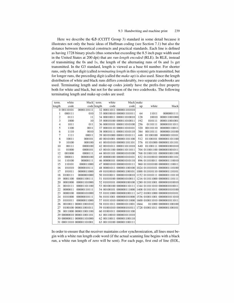
9.3 Handwriting and machine print 239

Here we describe the G3 (CCITT Group 3) standard in some detail because itillustrates not only the basic ideas of Huffman coding (see Section 7.1) but also thedistance between theoretical constructs and practical standards. Each line is definedas having 1728 binary pixels (thus somewhat exceeding the 8.5 inch page width usedin the United States at 200 dpi) that are run-length encoded (RLE). In RLE, insteadof transmitting the 0s and 1s, the length of the alternating runs of 0s and 1s gettransmitted. In the G3 standard, length is viewed as a base 64 number. For shorterruns, only the last digit (called terminating length in this system) gets transmitted, butfor longer runs, the preceding digit (called the make-up) is also used. Since the lengthdistribution of white and black runs differs considerably, two separate codebooks areused. Terminating length and make-up codes jointly have the prefix-free propertyboth for white and black, but not for the union of the two codebooks. The followingterminating length and make-up codes are used:

term. white black term. white black makelength code code length code code up white black

0 00110101 0000110111 32 00011011 0000011010101 000111 010 33 00010010 000001101011 64 11011 00000011112 0111 11 34 00010011 000011010010 128 10010 0000110010003 1000 10 35 00010100 000011010011 192 010111 0000110010014 1011 011 36 00010101 000011010100 256 0110111 0000010110115 1100 0011 37 00010110 000011010101 320 00110110 0000001100116 1110 0010 38 00010111 000011010110 384 00110111 0000001101007 1111 00011 39 00101000 000011010111 448 01100100 0000001101018 10011 000101 40 00101001 000001101100 512 01100101 00000011011009 10100 000100 41 00101010 000001101101 576 01101000 0000001101101

10 00111 0000100 42 00101011 000011011010 640 01100111 000000100101011 01000 0000101 43 00101100 000011011011 704 011001100 000000100101112 001000 0000111 44 00101101 000001010100 768 011001101 000000100110013 000011 00000100 45 00000100 000001010101 832 011010010 000000100110114 110100 00000111 46 00000101 000001010110 896 011010011 000000111001015 110101 000011000 47 00001010 000001010111 960 011010100 000000111001116 101010 0000010111 48 00001011 000001100100 1024 011010101 000000111010017 101011 0000011000 49 01010010 000001100101 1088 011010110 000000111010118 0100111 0000001000 50 01010011 000001010010 1152 011010111 000000111011019 0001100 00001100111 51 01010100 000001010011 1216 011011000 000000111011120 0001000 00001101000 52 01010101 000000100100 1280 011011001 000000101001021 0010111 00001101100 53 00100100 000000110111 1344 011011010 000000101001122 0000011 00000110111 54 00100101 000000111000 1408 011011011 000000101010023 0000100 00000101000 55 01011000 000000100111 1472 010011000 000000101010124 0101000 00000010111 56 01011001 000000101000 1536 010011001 000000101101025 0101011 00000011000 57 01011010 000001011000 1600 010011010 000000101101126 0010011 000011001010 58 01011011 000001011001 1664 011000 000000110010027 0100100 000011001011 59 01001010 000000101011 1728 010011011 000000110010128 0011000 000011001100 60 01001011 00000010110029 00000010 000011001101 61 00110010 00000101101030 00000011 000001101000 62 00110011 00000110011031 00011010 000001101001 63 00110100 000001100111

In order to ensure that the receiver maintains color synchronization, all lines must be-gin with a white run length code word (if the actual scanning line begins with a blackrun, a white run length of zero will be sent). For each page, first end of line (EOL,

240 9 Speech and handwriting

000000000001) is sent, followed by variable-length line codes, each terminated byEOL, with six EOLs at the end of the page. On the average, G3 compression reducesthe size of the image by a factor of 20.Exercise 9.4 Research the CCITT Group 4 (G4) standard, which also exploits someof the redundancy between successive lines of the scanned image and thereby im-proves compression by a factor of 2. Research JBIG and JBIG2, which generallyimprove G4 compression by another factor of 4.

Since the black and white runs give a good indication of the rough position of contentelements, the first step of page decomposition is often performed on RLE data, whichis generally sufficient for establishing the local horizontal and vertical directions andfor the appropriate grouping of titles, headers, footers, and other material set in a fontdifferent from the main body of the text. Adaptation to the directions inherent in thepage is called deskewing, and again it can take the form of transforming (rotating orshearing) the image or transforming the models. The tasks of deskewing and pagedecomposition are somewhat intertwined because the simplest page decompositionmethods work best when the image is not skewed. Unlike in speech recognition,where models that incorporate an explicit segmentation step have long been replacedby models that integrate the segmentation and the recognition step in a single HMMsearch, in OCR there is still very often a series of segmentation steps, first for textzones (i.e. rectangular windows that contain text only), then for lines, and finally forcharacters.

The search for text zones can proceed top-down or bottom-up. In the top-downapproach, we first count the black pixels in each row (column), obtaining a column(row) of blackness counts known as the projection profiles (see Wang and Srihari1989). These are generally sufficient for finding the headers and footers. Once theseare separated out, the vertical profile can be used to separate text columns, and oneach column horizontal profiles can be used to separate the text into lines. Besidessensitivity to skew, a big drawback of the method is that it presumes a regular, rect-angular arrangement of the page, and more fancy typography, such as text flowingaround a circular drawing, will cause problems. In the bottom-up approach, we be-gin with the smallest elements, connected components, and gradually organize themor their bounding boxes (the smallest rectangle entirely containing them) into largerstructures. By searching for the dominant peak in a histogram of vectors connectingeach component to its nearest neighbor, the skew of the document can be reliablydetected (Hashizume et al. 1986, O’Gorman 1993). Both the identification of con-nected components and the finding of nearest neighbors are computationally very ex-pensive steps, and once we are willing to spend the resources, other skew-insensitivemethods of segmenting text from images, such as the use of Gabor filters (Jain andBhattacharjee 1992) are also available.

Besides deskewing, there are several other normalization steps performed onthe entire image as needed; for example, xeroxing or scanning thick, bound docu-ments introduces perspective distortion at the edge of the page (see Kanungo et al.1993), and the vibrations of the scanner can cause blurring. Detection and removalof speckle noise (also known as salt-and-pepper noise because noise can take the

9.3 Handwriting and machine print 241

form of unwanted white pixels, not just black) is also best performed on the basisof estimating the noise parameters globally. Other normalization steps, in particularremoving distortions in the horizontal baseline caused by a loose paper forwardingmechanism (common in mechanical typewriters and low-quality scanners/faxes), arebetter performed line by line.

To the extent that small skew (generally within one degree) and simple rectangu-lar page layout are valid assumptions for the vast majority of holdings in digital li-braries, the less expensive top-down algorithms remain viable and have the advantagethat finding text lines and characters can generally proceed by the same steps. Formachine-printed input and for handprint (block letters, as opposed to cursive writ-ing), these steps reduce the problem to that of isolated character recognition. Herethe dominant technology is template matching, typically by neural nets or other train-able algorithms. Since direct matching of templates at the bitmap level, the methodused in the first commercially available OCR system in 1955, works well only forfixed fonts known in advance, attention turned early on to deriving a suitable set offeatures so that variants of the same character will map to close points in featurespace.

For isolated characters, the first step is generally size normalization; i.e. rescalingthe image to a standardized window. Since this window is typically much smallerthan the original (it can be as small as 5 by 7 for Latin, Cyrillic, and similar alphabets,16 by 20 for Oriental characters), the new pixels correspond to larger zones of theoriginal bounding box. The new pixel values are set to the average blackness of eachzone, so that the rescaled image will be grayscale (4–8 bits) even if the original wasbinary (Bokser 1992). Because characters can vary from the extremely narrow tothe extremely broad, the aspect ratio of the original bounding box is generally keptas a separate feature, together with the position of the bounding box relative to thebaseline so as to indicate the presence or absence of ascenders and descenders.

Besides absolute size, we also wish to normalize stroke width in handwrittencharacters and font weight in machine print. An elegant, and widely used, technologyfor this is mathematical morphology (MM), which is based on the dual operationsof erosion and dilation. We begin with a fixed set B � R2 called the structuringelement, typically a disk or square about the origin. The reflection of B , denoted OB ,is defined as f�xjx 2 Bg – for the typical structuring elements, symmetrical aboutthe origin, we have OB D B . The translation Bx of B by vector x is defined asfbCxjb 2 Bg. The dilation A˚B of A by B is defined as fxj OBx \A ¤ ;g, and theerosion AB of A by B is defined as fxjBx � Ag. Two MM operations defined ontop of these are the opening A ıB of A by B given by .AB/˚B and the closingA � B of A by B given by .A˚ B/ B . Finally, the boundary @A of A accordingto B is defined as A n .A B/.

What makes MM particularly useful for image processing is that all the opera-tions above remain meaningful if the sets A and B are composed of pixels (elementsof a tiling of R2). For example, if the structuring element B is chosen to be slightlysmaller than the regular printed dot (both periods at sentence end and dots over is),the operation .AıB/�B will filter out all salt-and-pepper noise below this size whileleaving the information-carrying symbols largely intact. By iterated erosion, we can

242 9 Speech and handwriting

also obtain the skeleton of an image, defined as the set of those points in the imagethat are equidistant from at least two points of the boundary. While in principle theskeleton should be an ideal replacement of characters with greater stroke width, inpractice skeletonization and all forms of thinning are quite sensitive to noise, evenafter despeckling. Noise is also a persistent problem for approaches based on chaincodes that express a simply connected two-dimensional shape in terms of its one-dimensional boundary.

In vertex chain coding, we apply the same principle to triangular, rectangular,and hexagonal tilings: we pick any vertex of the polygon that bounds the object andcount the number of pixels that are connected to the boundary at that vertex. Thetotal chain code is obtained by reading off these numbers sequentially following thepolygon counterclockwise. Several chain codes, all cyclic permutations of the samestring, could be obtained, depending on the vertex at which we start. For uniqueness,we pick the one that is minimal when interpreted as a number. This will make thecode rotation invariant.

Chain codes offer a relatively compact description of simply connected binaryimages, and efficient algorithms exist to compute many important properties of animage (such as its skew; see Kapogiannopoulos and Kalouptsidis 2002) based onchain codes for all connected components. However, for isolated character recogni-tion, chain codes are very brittle: many characters have holes, and features such as‘being n times connected’ (and in general all Betti numbers and other topologicalinvariants) are greatly affected by noise. In the analysis of handwriting, it is a par-ticularly attractive idea (already present in Eden 1961) to build a naturalistic modelalong the same lines we were all taught in first grade: t is a straight line down, curveto the right, cross near the top. Noise stands in the way of such structural decom-position approaches to a remarkable degree, and simple, robust features such as theheight contour, which is obtained from a line by computing the highest and the low-est black pixel in each column of pixels, turn out to be more helpful in OCR eventhough they clearly ignore structural features of the original such as loops.

Therefore it is particularly important to look for noise-robust features that pre-serve as many of the desirable invariance properties of chain codes as feasible.After size normalization, the character image fits in a fixed domain and can bethought of as a function f .x; y/ with value zero outside e.g. the unit circle (whichis mathematically more convenient than a rectangular bounding box). A typicalnormalization/feature extraction step is computing the central moments �pq de-fined in the usual manner by computing the x and y directional means x D’xf .x; y/dxdy=

’f .x; y/dxdy and y D

’yf .x; y/dxdy=

’f .x; y/dxdy

and defining

�pq D

“.x � x/p.y � y/qf .x; y/d.x � x/d.y � y/ (9.30)

Clearly, the central moments are invariant under arbitrary translation. Since themoment-generating function and the two-dimensional Fourier transform of f areessentially the same complex function viewed on the real and the imaginary axes, itcomes as little surprise that Fourier techniques, both discrete and continuous, play

9.3 Handwriting and machine print 243

the same pivotal role in the two-dimensional (handwriting signal) case that they haveplayed in the one-dimensional (speech signal) case.

To obtain features that are also invariant under rotation, we can express f interms of any orthogonal basis where rotation invariance is easily captured. One stan-dard method is to define the n;m radial polynomials Rnm.�/, where n is the orderof the polynomial, m is the winding number, n � jmj is assumed even, jmj < n by

Rnm.�/ D

n�jmj=2XsD0

.�1/s.n � s/Š�n�2s

sŠ�

nCjmj

2� s

�Š�

n�jmj

2� s

�Š

(9.31)

and define the n;m Zernike basis function Vnm.�; �/ as Vnm.�; �/ D Rnm.�/eim� .

These functions are orthogonal on the unit disk, with“x2Cy2�1

Vnm.x; y/Vpq.x; y/dxdy D�

nC 1ınpımq (9.32)

The Zernike moment Anm of a function f (already assumed size and translationnormalized) is given by

Anm D

“x2Cy2�1

f .x; y/Vnm.�; �/dxdy (9.33)

If g.�; �/ is obtained from f .�; �/ by rotation with angle ˛ (i.e. g.�; �/ D f .�; � �

˛/), the n;m-th Zernike moment of g is Anme�im˛ , where Anm was the n;m-th

Zernike moment of f . Thus, the absolute values jAnmj are rotation invariant. Noticethat fully rotation-invariant features are not ideally suited for OCR – for example,6 and 9 would get confused. A more important goal is the normalization of slant,both for the recognition of handwriting and for machine print that contains italicizedportions. Projection profiles, taken in multiple directions, give a good indication ofwriting slant and are often used.

Altogether, the computation of features for isolated characters often involves amixture of normalization and feature extraction steps that may end up producingmore data, as measured in bits, than were present in the original image. This is par-ticularly true in cases such as Zernike moments or other series expansion techniques(Fourier, wavelet, and similar techniques are often used), which could lead to a largenumber of terms limited only by two-dimensional versions of Theorem 9.1.1. In gen-eral, the goal is not simply data reduction but rather finding the features that providegood clustering of the data for VQ and other techniques the way Itakura-Saito diver-gence does for speech signals.

Typically, data reduction is accomplished by Karhunen-Loeve transformation,also known as principal component analysis (PCA). We begin with a set of (real orcomplex) feature vectors xi .1 � i � n/ with some high dimension N and seek tofind the projection P to d -dimensional space that retains as much of the variance inthe data as possible. To this end, we first compute the (empirical) mean of the dataset x D

1n

PniD1 xi and subtract it from all feature vectors (in practical applications,

the variances are also often normalized). The covariance matrix of the (now zero

244 9 Speech and handwriting

mean) vectors is symmetric (or Hermitian, if complex features are used) and thushas orthogonal eigenvectors. These are ordered according to decreasing size of theeigenvalues, and only the first d are kept. P projects the (zero mean) data on thesubspace spanned by these eigenvectors.

If the task is recognition, it is at least in principle possible for important infor-mation to be lost in PCA since the variability according to some critical feature maybe low. To account for this possibility, sometimes linear discriminant analysis (LDA;see Fisher 1936, 1937) is used, but the improvement over PCA is generally slightwhen LDA is just a preprocessing stage for some more complex recognition strategysuch as nearest neighbor classification. The advantage of LDA is in the fact that itwill derive a robust classifier in its own right and the training process, which usesonly the first and second moments of the distributions of xi , is very fast.Exercise 9.5�� Develop a handprint classifier using the NIST isolated characterdatabase available at http://www.nist.gov/srd/nistsd19.htm. Com-pare your results with the state of the art.

Most classification methods that work well for machine print and handprint run intoserious problems when applied to cursive writing because in the character identifica-tion stage it is very hard to recover from errors made in the segmentation stage. Thefilter- and projection-based page decomposition methods discussed here generalizereasonably well to cursive writing as far as segmentation into text blocks and linesis concerned, but segmenting a line into separate words and a word into separatecharacters based on these and similar methods is prone to very significant errors. Forcursive writing, the segmentation problem must be confronted the same way as inspeech recognition. To quote Halle and Stevens (1962:156),

The analysis procedure that has enjoyed the widest acceptance postulatesthat the listener first segments the utterance and then identifies the individualsegments with particular phonemes. No analysis scheme based on this prin-ciple has ever been successfully implemented. This failure is understandablein the light of the preceding account of speech production, where it was ob-served that segments of an utterance do not in general stand in a one-to-onerelation with the phonemes. The problem, therefore, is to devise a proce-dure which will transform the continuously-changing speech signal into adiscrete output without depending crucially on segmentation.

To this day, we do not have successful early segmentation, and not for lack of trying.Until the advent of HMMs, there were many systems based on the segmentation-classification-identification pipeline, but none of them achieved performance at thedesired level. Today, many of the design features deemed necessary by the prescientHalle-Stevens work, such as the use of generative language models for the lexiconand larger utterances or the pruning of alternatives by multiple passes, are built intoHMMs, but the main strength of these systems comes from two principal sources:first, that the recognition algorithm explores segmentation and classification alter-natives in parallel, and second, that the system is trainable. Parallelism means that

9.4 Further reading 245

HMMs are capable of considering all segmentation alternatives (hypothesizing ev-ery new frame as potentially beginning a new phoneme) without unduly burdening aseparate phoneme-level recognizer. Perhaps ironically, the best segmentation resultsare the ones obtained in the course of HMM recognition: rather than furnishing anessential first step of analysis, segment boundaries arise as a by-product of the fullanalysis.

9.4 Further reading

Viewed from a contemporary perspective, the great bulk of (digital) signal process-ing knowledge rests on a clean, elegant foundation of 19th century complex functiontheory and should be very accessible to mathematicians once the terminological andnotational gap between mathematics and electrical engineering is crossed.1 Yet therational reconstruction of the fundamentals presented here has little in common withthe actual historical development, which is better understood through major text-books such as Flanagan (1972) (for analog) and Rabiner and Schafer (1978) (forearly digital). In particular, Theorem 9.1.1 goes back to Whittaker (1915) but hasbeen rediscovered many times, most notably by Shannon and Weaver (1949).

In the theory of time series analysis, Pade approximation is known as the au-toregressive moving average (ARMA) model, with the all-pole case referred to asautoregressive (AR) and the all-zero case as moving average (MA); see e.g. Box andJenkins (1970). In digital signal processing, there are a wide variety of windowingfunctions in use (see e.g. Oppenheim and Schafer 1999), but for speech little im-provement, if any, results from replacing the standard Hamming window by otherwindowing functions. The importance of the fast Fourier transform can hardly beoverstated – see Brigham (1988) for a textbook devoted entirely to this subject. Eventhough harmonic analysis is a natural framework for dealing with speech, algorithmsthat relied on actually computing Fourier coefficients were considered impracticalbefore the modern rediscovery of the FFT (Cooley and Tukey 1965). We mentionhere that the FFT was already known to Gauss (see Heideman et al. 1984).

The standard introduction to homomorphic speech processing is Schafer and Ra-biner (1975), but the presentation here follows more closely the logic of Makhoul(1975). Cepstra, and the attendant syllable-reversal terminology, were introduced inBogert et al. (1963); see also Childers et al. (1977). Mel-cepstral features have ef-fectively replaced direct (time domain) LPC features, but linear prediction, eitherapplied in the quefrency domain or directly (as in the GSM 6.10 standard), remainsa standard data compression method in modern audio transmission.

The savings effected by the fast algorithm of Exercise 9.2 are trivial by today’sstandards since p is generally on the order of 101, so p3 gives less than 105 in-structions per second, while the chips embedded in contemporary cell phones areincreasingly capable of hundreds of MIPS. Note, however, that in the image do-main a variety of operations, such as adaptive binarization (setting the binarization

1 In particular, in engineering works we often find the imaginary unit i denoted by j .

246 9 Speech and handwriting

threshold according to local conditions; see Kamel and Zhao 1993), are still quiteexpensive.

For an overview of unsupervised clustering, see Everitt (1980) and Duda et al.(2000 Ch. 10), and for the supervised case, see Anderberg (1973). For Itakura-Saitodivergence, see Itakura (1975), and for its relation to Bregman divergences, seeMcAulay (1984), Wei and Gibson (2000), and Banerjee at al (2005). For optimaldecorrelation of cepstral features, see Demuynck et al. (1998). Tying techniques,which are critical for training high-quality HMMs, are discussed further in Jelinek(1997 Ch. 10). For speaker adaptation, see Richard Stern’s survey article on robustspeech recognition in Cole (1997, with a new edition planned for 2007).

Although somewhat dated, both Bunke and Wang (1997) and O’Gorman andKasturi (1995) offer excellent introductions to the many specialized topics relatedto OCR. For an overview of the early history, see Mori et al. (1992). For adaptivethresholding, see Sezgin and Sankur (2004). For page segmentation, see Antona-copoulos et al. (2005). Mathematical morphology was invented by Matheron andSerra (see Serra 1982); for various generalizations, see Maragos et al. (1996). For acomparison of skeletalization and thinning algorithms see Lee et al. (1991) and Lamet al. (1992). Chain codes were introduced by Freeman (1961). The vertex chain codepresented here is from Bribiesca (1999).

Moment normalization originated with Hu (1962). Zernike polynomials arise inthe study of wavefronts for optical systems with a central axis (Zernike 1934) andare widely used in opthalmology to this day. Their use in character recognition wasfirst proposed in Khotanzad and Hong (1990). For an overview of feature extractionmethods for isolated character recognition, see Trier et al. (1996). PCA and LDA arebasic tools in pattern recognition; see e.g. Duda et al. (2001 Sec. 3.8). For the use ofMMLR in dynamic handwriting recognition, see Senior and Nathan (1997), and forimage-based handwriting recognition, see Vinciarelli and Bengio (2002). The stateof the art in handwriting recognition is closely tracked by the International Workshopon Frontiers of Handwriting Recognition (IWFHR).

Early systems incorporating explicit rule-based segmentation steps are discussedin Makhoul (2006) from a historical perspective. In linguistic pattern recognition,trainability (called adaptive learning at the time) was first explored in early OCRwork (see Highleyman 1962, Munson 1968), but the practical importance and far-reaching theoretical impact of trainable models remained something of a trade secretto speech and OCR until the early 1990s, when Brown et al. (1990) demonstratedthe use of trainable models in machine translation. This is not to say that theoreticallinguistics ignored the matter entirely, and certainly the single most influential workof the period, Chomsky (1965), was very explicit about the need for grammaticalmodels to be learnable. Until the 1990s, theoretical linguistics focused on the rela-tionship of learnability and child language development (see e.g. Pinker 1984, 2ndrevised ed. 1996), mostly from the perspective of stimulus poverty, and it took theclear victory of trainable models over handcrafted rule systems in what was viewedas a core semantic competence, translation, to bring the pure symbol-manipulationand the statistical approaches together again (Pereira 2000).

10

Simplicity

Writing a textbook is a process that forces upon the author a neutral stance since itis clear that the student is best served by impartial analysis. Yet textbook authors canfeel as compelled to push their own intellectual agenda as authors of research papers,and for this final chapter I will drop the impersonal we together with its impliedneutrality and present a view of the overall situation in mathematical linguistics thatmakes no claims to being the standard view or even the view of a well-definableminority.

If one had to select a single theme running through this book, it would no doubtbe the emphasis on regular (finite state) structures. The classic results from this fieldoriginate with the work of Mealy (1955) on electric circuits and Kleene (1956) onnerve nets with discrete sets of inputs and outputs as opposed to the continuous inputsand outputs of perceptrons and contemporary neural nets. For the textbook writer, itwas reasonable to assume that at least a streamlined version of this material wouldbe familiar to the intended readership, as it is generally regarded as an essentialpart of the core computer science/discrete mathematics curriculum, and it was alsoreasonable to give short shrift to some of the more modern developments, especiallyto the use of (k-tape) finite state transducers in phonology/morphology, as these areamply covered in more specialized volumes such as Roche and Schabes (1997) andKornai (1999).

Yet I feel that, without this chapter, some of the impact of this work wouldbe lost on the reader. On the one hand, the methods pioneered by Mealy, Kleene,Schutzenberger, Krohn, Rhodes, Eilenberg, Angluin, and a host of others remain in-credibly versatile and highly generalizable as mathematical techniques. For example,much of the work on regular generalizations of FSA, both to transducers and to k-strings, is nothing but a rehash of the basic techniques relying on the identificationof the congruence classes (elements of the syntactic monoid) with automata states:if the (right)congruence has finite index, finite automata are available. But beforeturning to the issue of why these techniques are so highly generalizable, it shouldbe noted that there is an important aspect of these methods that has, to some ex-tent, been suppressed by the general turning of the tide against cybernetics, systems

248 10 Simplicity

theory, and artificial intelligence, namely the direct appeal to neurological modelsoriginating with Kleene.

As we all know, dealing with natural language is hard. It is hard from the stand-point of the child, who must spend many years acquiring a language (compare thistime span to that required for the acquisition of motor skills such as eating solids,walking, or swimming), it is hard for the adult language learner, it is hard for thescientist who attempts to model the relevant phenomena, and it is hard for the engi-neer who attempts to build systems that deal with natural language input or output.These tasks are so hard that Turing (1950) could rightly make fluent conversation innatural language the centerpiece of his test for intelligence. In more than half a cen-tury of work toward this goal, we have largely penetrated the outermost layer, speechproduction and perception, and we have done so by relying on learning algorithmsspecific to the Markovian nature of the signal. In spite of notable advances in theautomatic acquisition of morphology, in this next layer we are still at a stage wherespeech recognition was forty years ago, with handcrafted models quite comparable,and in some cases superior, to machine-learned models.

Returning briefly to the issue raised at the beginning of this book: what do wehave when a model is 70%, 95%, or even 99.99% correct? Isn’t a single contradictionor empirically false prediction enough to render a theory invalid? The answer tothe first question is clearly positive: contradictions must be managed carefully in ametatheory (multivalued logic) and cannot pervade the theory itself. But the answerto the second question is negative: a single wrong prediction, or even a great numberof wrong predictions, does not render the theory useless or invalid, a methodologicalpoint that has been repeatedly urged by Chomsky. To quantify this better, let us try toderive at least some rough estimates on the information content of linguistic theory.

There is a substantive body of information stored in the lexicon, which is clearlyirreducible in the sense that universal grammar will have little to say about the id-iosyncrasies of particular words or set phrases: a conservative estimate would be thesize of an abridged dictionary, 20,000–30,000 words, each requiring a few hundredunpredictable bits to encode their morphological, syntactic, and semantic aspects,for a total of about, say, a megabyte. Knowing that speech compression is alreadywithin a factor of five of the phonemic bitrate, we can conclude that the entire lexi-con, including phonetic/phonological information, is unlikely to exceed a couple ofmegabytes.

Traditional wisdom, largely confirmed by the practical experience of adult lan-guage learners, says that to know a language is to know the words, and in fact, fromthe middle ages until the 19th century, syntactic theory was viewed as a small ap-pendix to the main body of lexical and morphological knowledge. Perhaps a morerealistic estimate can be gathered from construction grammar, which relies on a fewdozen generic rules as opposed to thousands of specific constructions, or from Pan. ini,whose grammar is about 10% the size of his lexicons, the dhatupat.ha (about 2,000verbal roots) and the gan. apat.ha (about 20,000 nominal stems), even though he at-tempts neither detailed semantic analysis of content words nor exhaustive coveragein the lexicon. Be that as it may, a great deal of modern syntax seems to investigatethe recursive behavior of a few dozen constructions, likely encodable in less than

10 Simplicity 249

10 kilobytes, while the bulk of the training/learning effort is clearly directed at thenonrecursive (list-like) megabytes of data one needs to memorize in order to masterthe language.

As the reader who went through this book knows, mathematical linguistics isnot yet a unified theory: there are many ideas and fragments of theories, but there isnothing we could call a full theory of the domain. This is, perhaps, a reflection on thestate of linguistics itself, which is blessed with many great ideas but few that havefound good use beyond the immediate range of phenomena for which they weredeveloped. Notions such as the phoneme or the paradigm have had a tremendousimpact on anthropology, sociology, and literary theory, and some of the best workthat predates the still fashionable hodge-podge of ‘critical’ thought in the humanitiesclearly has its inspiration in these and similar notions of structural linguistics. Ifanything, language stands as a good example of a system “lacking a clear centralhierarchy or organizing principle and embodying extreme complexity, contradiction,ambiguity, diversity, interconnectedness, and intereferentiality” – the very definitionof the postmodern intellectual state according to Wikipedia. In these pages, in orderto gain clarity and to make a rigorous analysis possible, I have systematically chosenthe simplest versions of the problems, and even these no doubt embody extremecomplexity.

Is there, then, a single thread that binds mathematical linguistics together? Thisbook makes the extended argument that there is, and it is the attempt to find fastalgorithms. As all practicing engineers know, polynomial algorithms do not scale: forlarge problems only linear algorithms work. For example, Gaussian elimination, orany other O.N 3/ method, must be replaced for large but sparse matrices by rotationtechniques that scale linearly or nearly so with the amount of (nonzero) data. Sincefinite state methods are by their nature linear, improving the state of the art requiresa realignment of focus from the algebraically complex to the algebraically simple, inparticular to the noncounting finite state realm. The work is by no means done: thereis surprisingly much that we do not know about this domain, especially about theweighted versions of the models. For example, it is not known whether noncountinglanguages are pac learnable (under mild noise conditions). As Theorem 7.3.4 shows,there is little reason to believe that noncounting is the end of the story: to get a goodcharacterization of natural language syntax we need to establish further restrictionsso as to enable iitl learning. That said, noncounting still provides a valuable upperbound on the complexity of the problem.

The same drastic realignment of focus is called for in the case of semantics. Fartoo great attention has been lavished on complex systems with incredibly powerfuldeduction, to the detriment of investigating simpler, decidable calculi. There are amassive amount of facts for which a well-developed theory of semantics must ac-count, and in this domain we do not even have the beginnings of a good automaticacquisition strategy (Solomonoff-Levin universal learning is unlikely to scale). Yetit is clear that the standard approach of linguistics, ascribing as much complexity touniversal grammar (and, by implication, to the genetic makeup of humans) as canbe amortized over the set of possible languages, is not very promising for semantics.

250 10 Simplicity

The only words that can possibly yield to an approach from this direction belong inthe narrow class of physical sensations and emotional experiences.

In sum, it is not enough to stand on the shoulders of giants – we must also facein a better direction.

10.1 Previous reading

The best ideas in this book should be credited to people other than the author evenif no reference could be dug up. In particular, the heavy emphasis on noncountinglanguages originates with an apocryphal remark by John von Neumann: The braindoes not use the language of mathematics. The idea that VBTOs are first class entitiesis from William Lawvere, and the notion that linking is variable binding is fromlectures by Manfred Bierwisch. The concluding sentence follows from a bon mot ofAlan Kay.

References

Peter Aczel. 1988. Non-Well-Founded Sets. CSLI, Stanford, CA.Alfred V. Aho. 1968. Indexed grammars – an extension of context-free grammars.

Journal of the ACM, 15(4):647–671.Judith Aissen and David Perlmutter. 1983. Clause reduction in Spanish. In David

Perlmutter, editor, Studies In Relational Grammar, volume 1, pages 360–403.University of Chicago Press.

Kazimierz Ajdukiewicz. 1935. Die syntaktische konnexitat. Studia Philosophica,1:1–27.

Robin Allott. 1995. Sound symbolism. In Udo L. Figge, editor, Language In theWurm Glaciation, pages 15–38. Brockmeyer, Bochum.

Michael R. Anderberg. 1973. Cluster Analysis For Applications. Academic Press.John R. Anderson and Gordon H. Bower. 1973. Human Associative Memory. Win-

ston, Washington, DC.Stephen R. Anderson. 1982. Where is morphology? Linguistic Inquiry, 13:571–

612.Stephen R. Anderson. 1985. Phonology In the Twentieth Century: Theories of Rules

and Theories of Representations. University of Chicago Press.Stephen R. Anderson. 1992. A-Morphous Morphology. Cambridge University

Press.Stephen R. Anderson. 2000. Reflections on ‘On the phonetic rules of Russian’.

Folia Linguistica, 34(1–2):11–27.Dana Angluin. 1980. Inductive inference of formal languages from positive data.

Information and Control, 21:46–62.Dana Angluin. 1981. A note on the number of queries needed to identify regular

languages. Information and Control, 51:76–87.Dana Angluin. 1982. Inference of reversible languages. Journal of the ACM,

29:741–765.Dana Angluin. 1987. Learning regular sets from queries and counterexamples. In-

formation and Computation, 75:87–106.

252 References

Dana Angluin. 1992. Computational learning theory: Survey and selected bibliog-raphy. In Proceedings of STOC 92, pages 351–369.

Dana Angluin and Carl H. Smith. 1983. Inductive inference: Theory and methods.ACM Computing Surveys, 15(3):237–269.

Martin Anthony, Norman Biggs, and John Shawe-Taylor. 1990. The learnability offormal concepts. In Proceedings of the 3rd COLT, pages 246–257.

Apostolos Antonacopoulos, Basilios Gatos, and David Bridson. 2005. ICDAR2005page segmentation competition. In Proceedings of the 8th ICDAR, pages 75–79,Seoul, South Korea. IEEE Computer Society Press.

G. Aldo Antonelli. 1999. A directly cautious theory of defeasible consequence fordefault logic via the notion of general extension. Artificial Intelligence, 109(1-2):71–109.

Anthony Aristar. 1999. Typology and the Saussurean dichotomy. In E. Polome andC.F. Justus, editors, Language Change and Typological Variation: In Honor ofWinfred P. Lehmann. Journal of Indo-European Studies Monograph.

Mark Aronoff. 1976. Word Formation in Generative Grammar. MIT Press.Mark Aronoff. 1985. Orthography and linguistic theory: The syntactic basis of ma-

soretic Hebrew punctuation. Language, 61(1):28–72.John L. Austin. 1962. How to do things with Words. Clarendon Press, Oxford.Rainer Bauerle and Max J. Cresswell. 1989. Propositional attitudes. In F. Guenthner

and D.M. Gabbay, editors, Handbook of Philosophical Logic, volume IV, pages491–512. Reidel, Dordrecht.

Emmon Bach. 1980. In defense of passive. Linguistics and Philosophy, 3:297–341.Emmon Bach. 1981. Discontinuous constituents in generalized categorial gram-

mars. In Proceedings of the NELS, volume II, pages 1–12.Mark Baltin and Anthony Kroch. 1989. Alternative Conceptions of Phrase Struc-

ture. University of Chicago Press.Arindam Banerjee, Srujana Merugu, Inderjit S. Dhillon, and Joydeep Ghosh. 2005.

Clustering with Bregman divergences. Journal of Machine Learning Research,6:1705–1749.

Yehoshua Bar-Hillel. 1953. A quasi-arithmetical notation for syntactic description.Language, 29:47–58.

Yehoshua Bar-Hillel. 1964. Language and Information. Addison-Wesley.Yehoshua Bar-Hillel, Chaim Gaifman, and Eli Shamir. 1960. On categorial and

phrase structure grammars. Bulletin of the Research Council of Israel, 9F:1–16.Chris Barker. 2005. Variable-free semantics in 2005. ms, NYU.Chris Barker and Pauline Jacobson, editors. 2007. Direct Compositionality. Oxford

University Press.Jon Barwise and John Etchemendy. 1987. The Liar: An Essay in Truth and Circu-

larity. Oxford University Press.Jon Barwise and John Perry. 1983. Situations and Attitudes. MIT Press.Edwin L. Battistella. 1996. The Logic of Markedness. Oxford University Press.

References 253

Leonard E. Baum and Ted Petrie. 1966. Statistical inference for probabilistic func-tions of finite state Markov chains. Annals of Mathematical Statistics, 37:1554–1563.

Leonard E. Baum, Ted Petrie, George Soules, and Norman Weiss. 1970. A maxi-mization technique occurring in the statistical analysis of probabilistic functionsof Markov chains. Annals of Mathematical Statistics, 41(1):164–171.

Joffroy Beauquier and Loys Thimonier. 1986. Formal languages and Bernoulli pro-cesses. In J. Demetrovics, G.O.H. Katona, and A. Salomaa, editors, Algebra,Combinatorics, and Logic in Computer Science, pages 97–112. North-Holland,Amsterdam.

A. Melville Bell. 1867. Visible Speech. Simpkin and Marshall, London.Jerome R. Bellegarda and David Nahamoo. 1990. Tied mixture continuous param-

eter modeling for speech recognition. IEEE Transactions on Acoustics, Speech,and Signal Processing, 38(12):2033–2045.

Nuel D. Belnap. 1977. How a computer should think. In G. Ryle, editor, Contem-porary Aspects of Philosophy, pages 30–56. Oriel Press, Newcastle upon Tyne.

Nuel D. Belnap and L.E. Szabo. 1996. Branching space-time analysis of the GHZtheorem. Foundations of Physics, 26(8):989–1002.

W.R. Bennett. 1948. Spectra of quantized signals. Bell System Technical Journal,27:446–472.

Leo L. Beranek. 1949. Acoustic Measurements. Wiley, New York.Roger L. Berger. 1966. The Undecidability of the Domino Problem, volume 66.

Memoires of the American Mathematical Society, Providence, RI.Anne Bergeron and Sylvie Hamel. 2004. From cascade decompositions to bit-vector

algorithms. Theoretical Computer Science, 313:3–16.George Berkeley. 1734. The Analyst, or a Discourse addressed to an Infidel Mathe-

matician. Reprinted in W. Ewald, editor: From Kant to Hilbert: A Source Bookin the Foundations of Mathematics, Oxford University Press 1966.

Jean Berko. 1958. The child’s learning of English morphology. Word, 14:150–177.Jean Berstel. 1973. Sur la densite asymptotique de langages formels. In M. Nivat,

editor, Automata, Languages, and Programming, pages 345–358. North-Holland.Manfred Bierwisch. 1988. Thematic grids as the interface between syntax and se-

mantics. Lectures, Stanford, CA.Steven Bird and T. Mark Ellison. 1994. One-level phonology: Autosegmental repre-

sentations and rules as finite automata. Computational Linguistics, 20(1):55–90.Garrett Birkhoff. 1940. Lattice theory. American Mathematical Society Collo-

quium Publications, Providence, RI.James P. Blevins. 2003. Stems and paradigms. Language, 79(4):737–767.Juliette Blevins. 1995. The syllable in phonological theory. In John Goldsmith,

editor, Handbook of Phonology, pages 206–244. Blackwell, Oxford.Juliette Blevins and Sheldon P. Harrison. 1999. Trimoraic feet in Gilbertese.

Oceanic Linguistics, 38:203–230.Bernard Bloch and George L. Trager. 1942. Outline of Linguistic Analysis. Linguis-

tic Society of America, Baltimore.

254 References

Leonard Bloomfield. 1926. A set of postulates for the science of language. Lan-guage, 2:153–164.

Leonard Bloomfield. 1933. Language. George Allen and Unwin, London.Anselm Blumer, Andrzej Ehrenfeucht, David Haussler, and Manfred K. Warmuth.

1989. Learnability and the Vapnik-Chervonenkis dimension. Journal of theACM, 36(4):929–965.

Bruce P. Bogert, Michael J.R. Healy, and John W. Tukey. 1963. The quefrency alan-ysis of time series for echoes: cepstrum, pseudo-autocovariance, cross-cepstrum,and saphe cracking. In M. Rosenblatt, editor, Proceedings of the Symposium onTime Series Analysis, pages 209–243. Wiley.

Mindy Bokser. 1992. Omnidocument technologies. Proceedings of the IEEE,80(7):1066–1078.

George Box and Gwilym Jenkins. 1970. Time Series Analysis: Forecasting and Con-trol. Holden-Day, San Francisco.

Otto Bohtlingk. 1964. Pan. ini’s Grammatik. Georg Olms, Hildesheim.Michael Bottner. 2001. Peirce grammar. Grammars, 4(1):1–19.Ruth M. Brend and Kenneth L. Pike. 1976. Tagmemics, volume 2: Theoretical Dis-

cussion. Trends in Linguistics 2. Mouton, The Hague.Joan Bresnan. 1982. Control and complementation. In Joan Bresnan, editor, The

mental representation of grammatical relations, pages 282–390. MIT Press.Ernesto Bribiesca. 1999. A new chain code. Pattern Recognition, 32(2):235–251.E. Oran Brigham. 1988. The Fast Fourier Transform and its Applications. Prentice-

Hall.Ellen Broselow. 1995. The skeletal tier and moras. In John Goldsmith, editor, Hand-

book of Phonology, pages 175–205. Blackwell, Oxford.Peter Brown, John Cocke, Stephen Della Pietra, Vincent J. Della Pietra, Fredrick

Jelinek, John D. Lafferty, Robert L. Mercer, and Paul S. Roossin. 1990. A sta-tistical approach to machine translation. Computational Linguistics, 16:79–85.

Herman E. Buiskool. 1939. The Tripadi. Being an abridged English recast of Pur-vatrasiddham (an analytical-synthetical inquiry into the system of the last threechapters of Panini’s Astadhyayi). E.J. Brill, Leiden.

Horst Bunke and Patrick S.P. Wang, editors. 1997. Handbook of Character Recog-nition and Document Image Analysis. World Scientific, Singapore.

Oliver Cappe, Eric Moulines, and Tobias Ryden. 2005. Inference in Hidden MarkovModels. Springer.

Guy Carden. 1983. The non-finite = state-ness of the word formation component.Linguistic Inquiry, 14(3):537–541.

George Cardona. 1965. On Pan. ini’s morphophonemic principles. Language,41:225–237.

George Cardona. 1969. Studies in Indian grammarians I: The method of descriptionreflected in the Siva-sutras. Transactions of the American Philosophical Society,59(1):3–48.

George Cardona. 1970. Some principles of Pan. ini’s grammar. Journal of IndianPhilosophy, 1:40–74.

References 255

George Cardona. 1976. Some features of Pan. inian derivations. In H. Parret, ed-itor, History of Linguistic Thought and Contemporary Linguistics. de Gruyter,Berlin/New York.

George Cardona. 1988. Pan. ini: his Work and its Traditions, volume I. Motilal Ba-narsidass, New Delhi.

Greg Carlson and Francis J. Pelletier, editors. 1995. The Generic Book. Universityof Chicago Press.

Robert Carpenter and Glynn Morrill. 2005. Switch graphs for parsing type logicalgrammars. In Proceedings of the International Workshop on Parsing Technology,Vancouver. IWPT05.

Claudia Casadio, Philip J. Scott, and Robert A.G. Seely, editors. 2005. Languageand Grammar: Studies in Mathematical Linguistics and Natural Language.CSLI, Stanford CA.

Henrietta Cedergren and David Sankoff. 1974. Variable rules: performance as astatistical reflection of competence. Language, 50:335–355.

Gregory J. Chaitin. 1982. Godel’s theorem and information. International Journalof Theoretical Physics, 22:941–954.

David G. Champernowne. 1952. The graduation of income distributions. Econo-metrica, 20:591–615.

David G. Champernowne. 1953. A model of income distribution. Economic Jour-nal, 63:318–351.

David G. Champernowne. 1973. The Distribution of Income. Cambridge UniversityPress.

Bruce Chandler and Wilhelm Magnus. 1982. The History of Combinatorial GroupTheory: A Case Study in the History of Ideas. Springer.

Yuen Ren Chao. 1961. Graphic and phonetic aspects of linguistic and mathematicalsymbols. In R. Jakobson, editor, Structure of Language and its MathematicalAspects, pages 69–82. American Mathematical Society, Providence, RI.

Eugene Charniak. 1993. Statistical Language Learning. MIT Press.Colin Cherry. 1956. Roman Jakobson’s distinctive features as the normal coordi-

nates of a language. In Morris Halle, editor, For Roman Jakobson. Mouton, TheHague.

Colin Cherry, Morris Halle, and Roman Jakobson. 1953. Toward the logical descrip-tion of languages in their phonemic aspect. Language, 29:34–46.

Donald G. Childers, David P. Skinner, and Robert C. Kemerait. 1977. The cepstrum:A guide to processing. Proceedings of the IEEE, 65(10):1428–1443.

Noam Chomsky. 1956. Three models for the description of language. IRE Transac-tions on Information Theory, 2:113–124.

Noam Chomsky. 1957. Syntactic Structures. Mouton, The Hague.Noam Chomsky. 1959. On certain formal properties of grammars. Information and

Control, 2:137–167.Noam Chomsky. 1961. On the notion ‘rule of grammar’. In R. Jakobson, edi-

tor, Structure of Language and its Mathematical Aspects, pages 6–24. AmericanMathematical Society, Providence, RI.

256 References

Noam Chomsky. 1965. Aspects of the Theory of Syntax. MIT Press.Noam Chomsky. 1967. Degrees of grammaticalness. In J.A. Fodor and J.J. Katz,

editors, The Structure of Language, pages 384–389. Prentice-Hall.Noam Chomsky. 1970. Remarks on nominalization. In R. Jacobs and P. Rosen-

baum, editors, Readings in English Transformational Grammar, pages 184–221.Blaisdell, Waltham, MA.

Noam Chomsky. 1980. Rules and Representations. Columbia University Press.Noam Chomsky. 1981. Lectures on Government and Binding. Foris, Dordrecht.Noam Chomsky. 1995. The Minimalist Program. MIT Press.Noam Chomsky and Morris Halle. 1965a. Some controversial questions in phono-

logical theory. Journal of Linguistics, 1:97–138.Noam Chomsky and Morris Halle. 1968. The Sound Pattern of English. Harper and

Row, New York.Noam Chomsky and Howard Lasnik. 1993. Principles and parameters theory. In

J. Jacobs, editor, Syntax: An International Handbook of Contemporary Research,volume 1, pages 505–569. de Gruyter, Berlin.

Noam Chomsky and Marcel Paul Schutzenberger. 1963. The algebraic theory ofcontext-free languages. In P. Braffort and D. Hirschberg, editors, Computer Pro-gramming and Formal Systems, pages 118–161. North-Holland, Amsterdam.

Alexander Clark and Remy Eyraud. 2005. Identification in the limit of substitutablecontext-free languages. In S. Jain, H.U. Simon, and E.Tomita, editors, Proceed-ings of the 16th International Conference on Algorithmic Learning Theory (ALT2005), pages 283–296. Springer.

Robin Clark. 1994. Kolmogorov complexity and the information content of parame-ters. IRCS Report 94-17, Institute for Research in Cognitive Science, Universityof Pennsylvania.

George N. Clements. 1977. Vowel harmony in nonlinear generative phonology. InW.U. Dressler and O.E. Pfeiffer, editors, Phonologica 1976, pages 111–119. In-stitut fur Sprachwissenschaft der Universitat Innsbruck.

George N. Clements. 1985. The problem of transfer in nonlinear phonology. Cor-nell Working Papers in Linguistics, 5:38–73.

George N. Clements and Kevin C. Ford. 1979. Kikuyu tone shift and its synchronicconsequences. Linguistic Inquiry, 10:179–210.

George N. Clements and S. Jay Keyser. 1983. CV Phonology: A Generative Theoryof the Syllable. MIT Press.

Alan Cobham. 1969. On the base-dependence of sets of numbers recognizable byfinite automata. Mathematical Systems Theory, 3:186–192.

Ronald A. Cole, editor. 1997. Survey of the State of the Art in Human LanguageTechnology. Cambridge University Press.

N.E. Collinge. 1985. The Laws of Indo-European. Benjamins.Bernard Comrie, editor. 1990. The World’s Major Languages. Oxford University

Press.Confucius. 1979. The Analects. Penguin, Harmondsworth.

References 257

James W. Cooley and John W. Tukey. 1965. An algorithm for the machine calcula-tion of complex Fourier series. Mathematics of Computation, 19:297–301.

Robin Cooper. 1975. Montague’s Semantic Theory and Transformational Syntax.PhD thesis, University of Massachusetts, Amherst.

John Corcoran, William Hatcher, and John Herring. 1972. Variable binding termoperators. Zeitschrift fur mathematische Logik und Grundlagen der Mathematik,18:177–182.

Michael A. Covington. 1984. Syntactic Theory in the High Middle Ages. CambridgeUniversity Press.

David R. Cox and H. David Miller. 1965. The Theory of Stochastic Processes.Methuen, London.

Max J. Cresswell. 1985. Structured Meanings. MIT Press.Haskell B. Curry. 1961. Some logical aspects of grammatical structure. In R. Jakob-

son, editor, Structure of Language and its Mathematical Aspects, pages 56–68.American Mathematical Society, Providence, RI.

Haskell B. Curry and Robert Feys. 1958. Combinatory Logic I. North-Holland,Amsterdam.

James Cussens and Stephen G. Pulman. 2001. Grammar learning using inductivelogic programming. Oxford University Working Papers in Linguistics, Philologyand Phonetics, 6:31–45.

Steven B. Davis and Paul Mermelstein. 1980. Comparison of parametric representa-tions for monosyllabic word recognition in continuously spoken sentences. IEEETransactions on Acoustics, Speech, and Signal Processing, 28(4):357–366.

Max W. Dehn. 1912. Uber unendlich diskontinuierliche Gruppen. MathematischeAnnalen, 71:116–144.

Francois Dell and Mohamed Elmedlaoui. 1985. Syllabic consonants and syllabifica-tion in Imdlawn Tashlhiyt Berber. Journal of African Languages and Linguistics,7:105–130.

Francois Dell and Mohamed Elmedlaoui. 1988. Syllabic consonants in Berber:some new evidence. Journal of African Languages and Linguistics, 10:1–17.

Hans den Besten. 1985. The ergative hypothesis and free word order in Dutch andGerman. In J. Toman, editor, Studies in German Grammar, pages 23–64. Foris,Dordrecht.

Jim des Rivieres and Hector J. Levesque. 1986. The consistency of syntactical treat-ments of knowledge. In M. Vardi, editor, Theoretical aspects of reasoning aboutknowledge, pages 115–130. Morgan Kaufmann, Los Altos, CA.

Kris Demuynck, Jacques Duchateau, Dirk Van Compernolle, and Patrick Wambacq.1998. Improved feature decorrelation for HMM-based speech recognition. InProceedings of the ICSLP, volume VII, pages 2907–2910, Sydney, Australia.

Keith Devlin. 1991. Logic and Information. Cambridge University Press.Keith Devlin. 2001. The mathematics of information. ESSLLI Lecture Notes,

Helsinki.Luc Devroye, Laszlo Gyorfi, and Gabor Lugosi. 1996. A Probabilistic Theory of

Pattern Recognition. Springer.

258 References

Robert M.W. Dixon. 1994. Ergativity. Cambridge University Press.David Dowty, Robert Wall, and Stanley Peters. 1981. Introduction to Montague

Semantics. Reidel, Dordrecht.David Dowty. 1979. Word Meaning and Montague Grammar. Reidel, Dordrecht.David Dowty. 1985. On recent analyses of the semantics of control. Linguistics and

Philosophy, 8(3):291–331.David Dowty. 1991. Thematic proto-roles and argument selection. Language,

67:547–619.Erich Drach. 1937. Grundgedanken der deutschen Satzlehre. Diesterweg, Frank-

furt.Fred Dretske. 1981. Knowledge and the Flow of Information. MIT Press.Richard O. Duda, Peter E. Hart, and David G. Stork. 2000. Pattern Classification.

Wiley.Mark Durie. 1987. Grammatical relations in Acehnese. Studies in Language,

11(2):365–399.Umberto Eco. 1995. The Search for the Perfect Language. Blackwell, Oxford.Murray Eden. 1961. On the formalization of handwriting. In R. Jakobson, editor,

Structure of Language and its Mathematical Aspects, pages 83–88. AmericanMathematical Society, Providence, RI.

Andrzej Ehrenfeucht, David Haussler, Michael Kearns, and Leslie Valiant. 1989. Ageneral lower bound on the number of examples needed for learning. Informa-tion and Computation, 82:247–251.

Samuel Eilenberg. 1974. Automata, Languages, and Machines, volume A. Aca-demic Press.

P.D. Eimas, E.R. Siqueland, P. Jusczyk, and J. Vigorito. 1971. Speech perception ininfants. Science, 171:303–306.

Jason Eisner. 2001. Expectation semirings: Flexible EM for learning finite-statetransducers. In G. van Noord, editor, ESSLLI Workshop on Finite-State Methodsin Natural Language Processing, Helsinki.

Clarence A. Ellis. 1969. Probabilistic Languages and Automata. PhD thesis, Uni-versity of Illinois, Urbana.

Miklos Erdelyi-Szabo, Laszlo Kalman, and Agnes Kurucz. 2007. Towards a naturallanguage semantics without functors and operands. Journal of Logic, Languageand Information.

J.R. Estoup. 1916. Gammes Stenographiques. Institut Stenographique de France,Paris.

Brian Everitt. 1980. Cluster Analysis. Halsted Press, New York.Gunnar Fant. 1960. Acoustic Theory of Speech Production. Mouton, The Hague.Gilles Fauconnier. 1985. Mental Spaces. MIT Press.Fibonacci. 1202. Liber Abaci. Translated by L.E. Siegler. Springer (2002).Charles Fillmore. 1968. The case for case. In E. Bach and R. Harms, editors, Uni-

versals in Linguistic Theory, pages 1–90. Holt and Rinehart, New York.Charles Fillmore. 1977. The case for case reopened. In P. Cole and J.M. Sadock,

editors, Grammatical Relations, pages 59–82. Academic Press.

References 259

Charles Fillmore and Paul Kay. 1997. Berkeley Construction Grammar.http://www.icsi.berkeley.edu/˜kay/bcg/ConGram.html.

Kit Fine. 1985. Reasoning with Arbitrary Objects. Blackwell, Oxford.John Rupert Firth. 1948. Sounds and Prosodies. Transactions of the Philological

Society, 46:127–152.Ronald A. Fisher. 1936. The use of multiple measurements in taxonomic problems.

Annals of Eugenics, 7:179–188.Ronald A. Fisher. 1937. The statistical utilization of multiple measurements. Annals

of Eugenics, 8:376–385.James Flanagan. 1955. Difference limen for vowel formant frequency. Journal of

the Acoustical Society of America, 27:613–617.James Flanagan. 1972. Speech Analysis, Synthesis and Perception. Springer.Daniel P. Flickinger. 1987. Lexical Rules in the Hierarchical Lexicon. PhD Thesis,

Stanford University.Christophe Costa Florencio. 2003. Learning Categorial Grammars. PhD Thesis,

Universiteit Utrecht.William A. Foley and Robert van Valin. 1984. Functional Syntax and Universal

Grammar. Cambridge University Press.Carol A. Fowler and Dawn J. Dekle. 1991. Listening with eye and hand: Crossmodal

contributions to speech perception. Journal of Experimental Psychology: HumanPerception and Performance, 17:816–828.

Herbert Freeman. 1961. On the encoding of arbitrary geometric configurations. IRETransactions on Electronic Computers, 10:260–268.

Gottlob Frege. 1879. Begriffsschrift: eine der arithmetischen nachgebildete Formel-sprache des reinen Denkens. L. Nebert, Halle.

Osamu Fujimura, S. Kiritani, and H. Ishida. 1973. Computer controlled radiographyfor observation of movements of articulatory and other human organs. ComputerBiological Medicine, 3:371–384.

Sadaoki Furui. 1986. Speaker-independent isolated word recognition using dynamicfeatures of speech spectrum. IEEE Transactions on Acoustics, Speech, and Sig-nal Processing, 34(1):52–59.

Peter Gacs. 2003. Lecture notes on descriptional complexity and randomness. ms,Boston University.

Chaim Gaifman. 1965. Dependency systems and phrase-structure systems. Infor-mation and Control, 8:304–337.

L.T.F. Gamut. 1991. Logic, Language, and Meaning. University of Chicago Press.Gerald Gazdar. 1981. Unbounded dependencies and coordinate structure. Linguistic

Inquiry, 12:155–184.Gerald Gazdar, Ewan Klein, Geoffrey K. Pullum, and Ivan A. Sag. 1985. General-

ized Phrase Structure Grammar. Blackwell, Oxford.Matthew L. Ginsberg. 1986. Multi-valued logics. In Matthew L. Ginsberg, editor,

Readings in Non-monotonic Reasoning, pages 251–255. Morgan Kaufmann, SanMateo, CA.

260 References

Matthew L. Ginsberg, editor. 1986a. Readings in Non-monotonic Reasoning. Mor-gan Kauffman, San Mateo, CA.

Abraham Ginzburg. 1968. Algebraic Theory of Automata. Academic Press.Henry A. Gleason. 1961. Genetic relationship among languages. In R. Jakobson,

editor, Structure of Language and its Mathematical Aspects, pages 179–189.American Mathematical Society, Providence, RI.

Cliff Goddard. 2002. The search for the shared semantic core of all languages. InCliff Goddard and Anna Wierzbicka, editors, Meaning and Universal Grammar– Theory and Empirical Findings, volume 1, pages 5–40. Benjamins.

Rob W.N. Goedemans, Harry G. van der Hulst, and Ellis M. Visch. 1996. StressPatterns of the World. Part 1: Background. Holland Academic Graphics, TheHague.

E. Mark Gold. 1967. Language identification in the limit. Information and Control,10:447–474.

E. Mark Gold. 1978. Complexity of automaton identification from given data. In-formation and Control, 37(3):302–320.

John A. Goldsmith. 1976. Autosegmental Phonology. PhD thesis MIT.John A. Goldsmith. 1990. Autosegmental and Metrical Phonology. Blackwell,

Cambridge, MA.John Goldsmith and Gary Larson. 1990a. Local modeling and syllabification. In

M. Noske, K. Deaton, and M. Ziolkowski, editors, CLS 26 Parasession on theSyllable in Phonetics and Phonology, pages 129–142. Chicago Linguistic Soci-ety.

Raymond G. Gordon, Jr. 2005. Ethnologue: Languages of the World. SIL Interna-tional, Dallas, TX.

Robert M. Gray and E.D. Karnin. 1982. Multiple local optima in vector quantizers.IEEE Transactions on Information Theory, 28(2):256–261.

Joseph H. Greenberg. 1963. Some universals of grammar with particular referenceto the order of meaningful elements. In J.H. Greenberg, editor, Universals ofHuman Language, pages 73–113. MIT Press.

Barbara B. Greene and Gerald M. Rubin. 1971. Automatic grammatical tagging ofEnglish. Department of Linguistics, Brown University, Providence, RI, ms.

Maurice Gross. 1972. Mathematical Models in Linguistics. Prentice-Hall.Jozef Gruska. 1997. Foundations of Computing. Thomson International Computer

Press.Pierre Guiraud. 1954. Les characteres statistiques du vocabulaire. Presses Univer-

sitaires de France, Paris.Kenneth Hale. 1983. Warlpiri and the grammar of non-configurational languages.

Natural Language and Linguistic Theory, 1:5–47.Morris Halle. 1961. On the role of simplicity in linguistic descriptions. In R. Jakob-

son, editor, Structure of Language and its Mathematical Aspects, pages 89–94.American Mathematical Society, Providence, RI.

Morris Halle. 1964. On the bases of phonology. In J.A. Fodor and J. Katz, editors,The Structure of Language, pages 324–333. Prentice-Hall.

References 261

Morris Halle. 1983a. Distinctive features and their articulatory implementation.Natural Language and Linguistic Theory, 1:91–107.

Morris Halle and George N. Clements. 1983. Problem Book in Phonology. MITPress.

Morris Halle and Samuel Jay Keyser. 1971. English Stress: Its Growth and Its Rolein Verse. Harper and Row, New York.

Morris Halle and Peter Ladefoged. 1988. Some major features of the internationalphonetic alphabet. Language, 64:577–582.

Morris Halle and Ken Stevens. 1962. Speech recognition: A model and a programfor research. IRE Transactions on Information Theory, 49:155–159.

Michael Hammond. 1987. Hungarian cola. Phonology Yearbook, 4:267–269.Michael Hammond. 1995. Metrical phonology. Annual Review of Anthropology,

24:313–342.Zellig Harris. 1951. Methods in Structural Linguistics. University of Chicago Press.Zellig Harris. 1957. Coocurence and transformation in liguistic structure. Lan-

guage, 33:283–340.Randy Allen Harris. 1995. The Linguistics Wars. Oxford University Press.Michael A. Harrison. 1978. Introduction to Formal Language Theory. Addison-

Wesley.Ralph V.L. Hartley. 1928. Transmission of information. Bell System Technical Jour-

nal, 7:535–563.Akihide Hashizume, Pen-Shu Yeh, and Azriel Rosenfeld. 1986. A method of detect-

ing the orientation of aligned components. Pattern Recognition Letters, 4:125–132.

Trevor Hastie, Robert Tibshirani, and Jerome Friedman. 2001. Elements of Statisti-cal Learning: Data Mining, Inference, and Prediction. Springer.

John A. Hawkins. 1983. World Order Universals. Academic Press.Patrick J. Hayes. 1978. The Naive Physics Manifesto. Institut Dalle Molle, Geneva.Bruce Hayes. 1980. A Metrical Theory of Stress Rules. PhD thesis, MIT.Bruce Hayes. 1995. Metrical Stress Theory. University of Chicago Press.Harold S. Heaps. 1978. Information Retrieval – Computational and Theoretical

Aspects. Academic Press.Jeffrey Heath. 1987. Ablaut and Ambiguity: Phonology of a Moroccan Arabic Di-

alect. State University of New York Press, Albany.Michael T. Heideman, Don H. Johnson, and C. Sidney Burrus. 1984. Gauss and the

history of the FFT. IEEE Acoustics, Speech, and Signal Processing Magazine,1:14–21.

Irene Heim. 1982. The Semantics of Definite and Indefinite Noun Phrases. PhDthesis, University of Massachusetts, Amherst, MA.

Steve J. Heims. 1991. The Cybernetics Group, 1946–1953. MIT Press.Leon Henkin. 1950. Completeness in the theory of types. Journal of Symbolic

Logic, 15:81–91.Jacques Herbrand. 1930. Recherches sur la theorie de la demonstration. PhD thesis,

Paris.

262 References

Gustav Herdan. 1960. Type-Token Mathematics. Mouton, The Hague.Gustav Herdan. 1966. The Advanced Theory of Language as Choice and Chance.

Springer.Hynek Hermansky. 1990. Perceptual linear predictive (PLP) analysis of speech.

Journal of the Acoustical Society of America, 87(4):1738–1752.Hynek Hermansky, Nelson Morgan, Aruna Bayya, and Phil Kohn. 1991. RASTA-

PLP speech analysis. US West Advanced Technologies TR-91-069.Susan R. Hertz. 1982. From text-to-speech with SRS. Journal of the Acoustical

Society of America, 72:1155–1170.Wilbur H. Highleyman. 1962. Linear decision functions with application to pattern

recognition. Proceedings of the IRE, 50:1501–1514.Henry Hiz. 1961. Congrammaticality, batteries of transformations and grammatical

categories. In R. Jakobson, editor, Structure of Language and its MathematicalAspects, pages 43–50. American Mathematical Society, Providence, RI.

Louis Hjelmslev. 1961. Prolegomena to a Theory of Language. University of Wis-consin Press, Madison.

Robert D. Hoberman. 1987. Emphasis (pharyngealization) as an autosegmental har-mony feature. In A. Bosch, B. Need, and E. Schiller, editors, Parasession onAutosegmental and Metrical Phonology, volume 23, pages 167–181. CLS.

Charles Hockett. 1960. Logical considerations in the study of animal communica-tion. In W.E. Lanyon and W.N. Tavolga, editors, Animal Sounds and Communi-cations, pages 392–430. American Institute of Biological Sciences, Washington,DC.

Fred W. Householder. 1965. On some recent claims in phonological theory. Journalof Linguistics, 1:13–34.

Fred W. Householder. 1966. Phonological theory: a brief comment. Journal of Lin-guistics, 2:99–100.

Ming-Kuei Hu. 1962. Visual pattern recognition by moment invariants. IRE Trans-actions on Information Theory, 49:179–187.

Geoffrey J. Huck and John A. Goldsmith. 1995. Ideology and Linguistics Theory:Noam Chomsky and the Deep Structure Debates. Routledge, London.

Richard A. Hudson. 1990. English Word Grammar. Blackwell, Oxford.M. Sharon Hunnicutt. 1976. Phonological rules for a text to speech system. Ameri-

can Journal of Computational Linguistics, Microfiche 57:1–72.James R. Hurford. 1975. The Linguistic Theory of Numerals. Cambridge University

Press.Rini Huybregts. 1976. Overlapping dependencies in Dutch. Utrecht Working Papers

in Linguistics, 1:224–265.Larry M. Hyman. 1975. Phonology: Theory and Analysis. Holt, Rinehart, Winston,

New York.Larry M. Hyman. 1982. The representation of nasality in Gokana. In H. van der

Hulst and N. Smith, editors, The Structure of Phonological Representation, pages111–130. Foris, Dordrecht.

William J. Idsardi. 2006. Misplaced optimism. Rutgers Optimality Archive, 840.

References 263

Neil Immerman. 1988. Nondeterministic space is closed under complementation.SIAM Journal of Computing, 17(5):935–938.

H. Inose, Y. Yasuda, and J. Murakami. 1962. A telemetering system by code manip-ulation – delta-sigma modulation. IRE Transactions on Space Electronics andTelemetry, 8:204–209.

Fumitada Itakura. 1975. Minimum prediction residual principle applied to speechrecognition. IEEE Transactions on Acoustics, Speech, and Signal Processing,23:67–72.

Ray S. Jackendoff. 1972. Semantic Interpretation in Generative Grammar. MITPress.

Ray S. Jackendoff. 1977. X-bar Syntax: A Study of Phrase Structure. MIT Press.Ray S. Jackendoff. 1983. Semantics and Cognition. MIT Press.Ray S. Jackendoff. 1990. Semantic Structures. MIT Press.Pauline Jacobson. 1990. Raising as function composition. Linguistics and Philoso-

phy, 13(4):423–475.Pauline Jacobson. 1999. Towards a variable-free semantics. Linguistics and Philos-

ophy, 22:117–184.Anil K. Jain and Sushil Bhattacharjee. 1992. Text segmentation using Gabor filters

for automatic document processing. Machine Vision and Applications, 5:169–184.

Roman Jakobson. 1936. Beitrag zur allgemeinen Kasuslehre. Travaux du Cerclelinguistique de Prague.

Roman Jakobson. 1941. Kindersprache, Aphasie, und allgemeine Lautgesetze. Up-psala Universitets Arsskrift, Uppsala.

Roman Jakobson. 1957. Mufaxxama – the emphatic phonemes in Arabic. In E. Pul-grim, editor, Studies Presented to Joshua Whatmough. Mouton, The Hague.

Roman Jakobson, editor. 1961. Structure of Language and its Mathematical As-pects. American Mathematical Society, Providence, RI.

Roman Jakobson, Gunnar Fant, and Morris Halle. 1952. Preliminaries to SpeechAnalysis: The Distinctive Features and Their Correlates. MIT Press.

Theo M.V. Janssen. 1997. Compositionality. In J. van Benthem, editor, Handbookof Logic and Language, pages 414–474. Elsevier.

Nikil S. Jayant and Peter Noll. 1984. Digital Coding of Waveforms: Principles andApplications to Speech and Video. Prentice-Hall.

Frederick Jelinek. 1997. Statistical Methods for Speech Recognition. MIT Press.Otto Jespersen. 1897. Fonetik. Det Schubotheske Forlag, Copenhagen.Otto Jespersen. 1924. The Philosophy of Grammar. George Allen and Unwin, Lon-

don.Stig Johansson, Eric Atwell, Roger Garside, and Geoffrey Leech. 1986. The Tagged

LOB Corpus: Users’ Manual. ICAME: The Norwegian Computing Centre forthe Humanities.

Ch. Douglas Johnson. 1970. Formal aspects of phonological representation. PhDthesis, UC Berkeley.

264 References

Neil D. Jones. 1966. A survey of formal language theory. University of WesternOntario Computer Science Tech Report 3, London, ON.

S.D. Joshi and Saroja Bhate. 1984. Fundamentals of Anuvrtti. Poona UniversityPress.

Aravind K. Joshi. 2003. Tree adjoining grammars. In R. Mitkov, editor, Handbookof Computational Linguistics, pages 483–500. Oxford University Press.

Daniel Jurafsky and James H. Martin. 2000. Speech and Language Processing.Prentice-Hall.

Daniel Kahn. 1976. Syllable-based Generalizations in English Phonology. PhDthesis, MIT.

Ellen Kaisse and Sharon Hargus. 1993. Introduction. In Ellen Kaisse and SharonHargus, editors, Studies in Lexical Phonology, pages 1–19. Academic Press.

Mohamed Kamel and Aiguo Zhao. 1993. Extraction of binary character/graphicsimages from grayscale document images. Graphical Models and Image Pro-cessing, 55:203–217.

Hans Kamp. 1981. A theory of truth and semantic representation. In J.A.G. Groe-nendijk, T.M.V. Jansen, and M.B.J. Stokhof, editors, Formal Methods in theStudy of Language, pages 277–322. Mathematisch Centrum, Amsterdam.

Makoto Kanazawa. 1996. Identification in the limit of categorial grammars. Journalof Logic, Language and Information, 5(2):115–155.

Tapas Kanungo, Robert M. Haralick, and Ishin T. Phillips. 1993. Global and localdocument degradation models. In Proceedings of the 2nd ICDAR, pages 730–734.

Ronald M. Kaplan and Martin Kay. 1994. Regular models of phonological rulesystems. Computational Linguistics, 20:331–378.

David Kaplan. 1978. On the logic of demonstratives. Journal of PhilosophicalLogic, 8:81–98.

David Kaplan. 1989. Demonstratives. In J. Almog, J. Perry, and H. Wettstein, edi-tors, Themes from Kaplan, pages 481–563. Oxford University Press.

George S. Kapogiannopoulos and Nicholas Kalouptsidis. 2002. A fast high preci-sion algorithm for the estimation of skew angle using moments. In M. H. Hamza,editor, Proceedings of the Signal Processing, Pattern Recognition, and Applica-tions (SPPRA 2002), pages 275–279, Calgary, AB. Acta Press.

Richard M. Karp. 1972. Reducibility among combinatorial problems. In R. Millerand J.W. Thatcher, editors, Complexity of Computer Computations, pages 85–104. Plenum Press, New York.

Lauri Karttunen. 1995. The replace operator. In Proceedings of ACL95, pages 16–23.

Paul Kay. 2002. An informal sketch of a formal architecture for construction gram-mar. Grammars, 5:1–19.

Paul Kay and Chad K. McDaniel. 1979. On the logic of variable rules. Language inSociety, 8:151–187.

Michael Kearns and Leslie Valiant. 1989. Cryptographic limitations on learningBoolean formulae and finite automata. In Proceedings of the 21st Annual ACM

References 265

Symposium on Theory of Computing, pages 433–444.Aleksandr I. Khinchin. 1957. Mathematical Foundations of Information Theory.

Dover, New York.Alireza Khotanzad and Yaw Hua Hong. 1990. Invariant image recognition by

Zernike moments. IEEE Transactions on Pattern Analysis and Machine Intel-ligence, 12(5):489–497.

Paul Kiparsky. 1968. Linguistic universals and linguistic change. In E. Bach andR. Harms, editors, Universals in Linguistic Theory, pages 171–202. Holt, NewYork.

Paul Kiparsky. 1979. Pan. ini as a Variationist. MIT Press and Poona UniversityPress, Cambridge and Poona.

Paul Kiparsky. 1982. From cyclic phonology to lexical phonology. In H. van derHulst and N. Smith, editors, The structure of phonological representations, I,pages 131–175. Foris, Dordrecht.

Paul Kiparsky. 1982a. The ordering of rules in Pan. ini’s grammar. In Some Theo-retical Problems in Pan. ini’s Grammar, Post-graduate and Research DepartmentSeries, pages 77–121. Bhandarkar Oriental Research Institute, Poona.

Paul Kiparsky. 1987. Morphosyntax. ms, Stanford University.Paul Kiparsky. 2002. On the Architecture of Pan. ini’s grammar. ms, Stanford Uni-

versity.Paul Kiparsky. 2006. Paradigms and opacity. CSLI and University of Chicago

Press.Georg Anton Kiraz. 2001. Computational Nonlinear Morphology with Emphasis on

Semitic Languages. Cambridge University Press.Charles Kisseberth. 1970. On the functional unity of phonological rules. Linguistic

Inquiry, 1:291–306.Thomas Klammer and Muriel R. Schulz. 1996. Analyzing English Grammar. Allyn

and Bacon, Boston.Dennis H. Klatt. 1980. SCRIBER and LAFS: Two new approaches to speech

analysis. In Wayne Lea, editor, Trends in Speech Recognition, pages 529–555.Prentice-Hall.

Dennis H. Klatt. 1987. Review of text-to-speech conversion for English. Journal ofthe Acoustical Society of America, 82(3):737–793.

Stephen C. Kleene. 1956. Representation of events in nerve nets and finite automata.In C. Shannon and J. McCarthy, editors, Automata Studies, pages 3–41. PrincetonUniversity Press.

W. Klein, Reinier Plomp, and Louis C.W. Pols. 1970. Vowel spectra, vowel spaces,and vowel identification. Journal of the Acoustical Society of America, 48:999–1009.

Donald E. Knuth. 1971. The Art of Computer Programming. Addison-Wesley.Martha Kolln. 1994. Understanding English Grammar. MacMillan, New York.Andrei N. Kolmogorov. 1965. Three approaches to the quantitative definition of

information. Problems of Information Transmission, 1:1–7.

266 References

Andras Kornai. 1985. Natural languages and the Chomsky hierarchy. In MargaretKing, editor, Proceedings of the 2nd European ACL Conference, pages 1–7.

Andras Kornai. 1987. Finite state semantics. In U. Klenk, P. Scherber, andM. Thaller, editors, Computerlinguistik und philologische Datenverarbeitung,pages 59–70. Georg Olms, Hildesheim.

Andras Kornai. 1995. Formal Phonology. Garland Publishing, New York.Andras Kornai. 1996. Analytic models in phonology. In J. Durand and B. Laks,

editors, Current Trends in Phonology: Models and Methods, volume 2, pages395–418. CNRS, ESRI, Paris X, Paris.

Andras Kornai. 1998. Quantitative comparison of languages. Grammars, 1(2):155–165.

Andras Kornai, editor. 1999. Extended Finite State Models of Language. CambridgeUniversity Press.

Andras Kornai. 1999a. Zipf’s law outside the middle range. In J. Rogers, editor,Proceedings of the Sixth Meeting on Mathematics of Language, pages 347–356.University of Central Florida.

Andras Kornai. 2002. How many words are there? Glottometrics, 2(4):61–86.Andras Kornai and Geoffrey K. Pullum. 1990. The X-bar theory of phrase structure.

Language, 66:24–50.Andras Kornai and Zsolt Tuza. 1992. Narrowness, pathwidth, and their application

in natural language processing. Discrete Applied Mathematics, 36:87–92.Frederik H.H. Kortlandt. 1973. The identification of phonemic units. La Linguis-

tique, 9(2):119–130.Kimmo Koskenniemi. 1983. Two-level model for morphological analysis. In Pro-

ceedings of IJCAI-83, pages 683–685.C.H.A. Koster. 1970. Two-level grammars. Seminar on Automata Theory and Math-

ematical Linguistics, 11.Marcus Kracht. 2003. The Mathematics of Language. Mouton de Gruyter, Berlin.Marcus Kracht. 2007. Counter-free languages are not learnable. ms, UCLA.Angelika Kratzer. 1995. Stage level and individual level predicates. In G. Carlson

and F.J. Pelletier, editors, The Generic Book. University of Chicago Press.Saul A. Kripke. 1972. Naming and necessity. In D. Davidson, editor, Semantics of

Natural Language, pages 253–355. D. Reidel, Dordrecht.Saul A. Kripke. 1975. Outline of a theory of truth. Journal of Philosophy, 72:690–

716.Anthony Kroch. 1994. Morphosyntactic variation. In K. Beals, editor, Proceedings

of the CLS 30 Parasession on Variation and Linguistic Theory, volume 2, pages180–201. Chicago Linguistic Society.

Kenneth Krohn and John Rhodes. 1965. Algebraic theory of machines. I. Primedecomposition theorem for finite semigroups and machines. Transactions of theAmerican Mathematical Society, 116:450–464.

Henry Kucera and Nelson Francis, editors. 1967. Computational Analysis ofPresent-Day American English. Brown University Press, Providence, RI.

References 267

Patrica K. Kuhl and James D. Miller. 1975. Speech perception by the chinchilla:voiced-voiceless distinction in alveolar plosive consonants. Science, 190:69–72.

Marco Kuhlmann. 2005. Mildly Context-Sensitive Dependency Languages. Pro-gramming Systems Lab, Saarland University.

Werner Kuich. 1970. On the entropy of context-free languages. Information andControl, 16:173–200.

Werner Kuich and Arto Salomaa. 1986. Semirings, Automata, Languages. Springer.William Labov. 1966. The social stratification of English in New York City. Center

for Applied Linguistics, Washington, DC.William Labov. 1981. Resolving the neogrammarian controversy. Language,

57:267–308.William Labov. 1994. Principles of Linguistic Change: Internal Factors. Blackwell,

Oxford.Louisa Lam, Seong-Whan Lee, and Ching Y. Suen. 1992. Thinning methodologies

– a comprehensive survey. IEEE Transactions on Pattern Analysis and MachineIntelligence, 14(9):869–885.

Joachim Lambek. 1958. The mathematics of sentence structure. American Mathe-matical Monthly, 65:154–170.

Joachim Lambek. 1961. On the calculus of syntactic types. In R. Jakobson, editor,Structure of Language and its Mathematical Aspects, pages 166–178. AmericanMathematical Society, Providence, RI.

Joachim Lambek. 2004. A computational approach to English grammar. Syntax.Ronald Langacker. 1982. Space grammar, analyzability, and the English passive.

Language, 58:22–80.Ronald Langacker. 1987. Foundations of Cognitive Grammar, volume 1. Stanford

University Press.Ronald Langacker. 1991. Foundations of Cognitive Grammar, volume 2. Stanford

University Press.D. Terence Langendoen and Paul M. Postal. 1984. The vastness of natural language.

Blackwell, Oxford.Shalom Lappin. 1996. Generalized quantifiers, exception phrases, and logicality.

Journal of Semantics, 13:197–220.William Leben. 1973. Suprasegmental phonology. PhD thesis, MIT.Ki-Seung Lee and Richard V. Cox. 2001. A very low bit rate speech coder based

on a recognition/synthesis paradigm. IEEE Transactions on Speech and AudioProcessing, 9(5):482–491.

Seong-Whan Lee, Louisa Lam, and Chin Y. Suen. 1991. Performance evaluationof skeletonization algorithms for document image processing. In Proceedings ofICDAR’91, pages 272–282.

Geoffrey Leech, Roger Garside, and Michael Bryant. 1994. CLAWS4: the taggingof the British National Corpus. In Proceedings of the 15th International Confer-ence on Computational Linguistics, pages 622–628, Kyoto, Japan.

268 References

Karel de Leeuw, Edward F. Moore, Claude E. Shannon, and N. Shapiro. 1956. Com-putability by probabilistic machines. In C.E. Shannon and J. McCarthy, editors,Automata studies, pages 185–212. Princeton University Press.

Christopher J. Leggetter and Philip C. Woodland. 1995. Maximum likelihood linearregression for speaker adaptation of continuous density Hidden Markov Models.Computer Speech and Language, 9:171–185.

Ilse Lehiste. 1970. Suprasegmentals. MIT Press.Willem J.M. Levelt. 1974. Formal Grammars in Linguistics and Psycholinguistics,

volume 1–3. Mouton, The Hague.Beth Levin. 1993. English Verb Classes and Alternations: A Preliminary Investiga-

tion. University of Chicago Press.Beth Levin and Malka Rappaport Hovav. 2005. Argument Realization. Cambridge

University Press.Juliette Levin. 1985. A Metrical Theory of Syllabicity. PhD thesis, MIT.Ming Li and Paul Vitanyi. 1995. A new approach to formal language theory by

kolmogorov complexity. SIAM J. Comput, 24(2):398–419.Ming Li and Paul Vitanyi. 1997. An Introduction to Kolmogorov Complexity and Its

Applications. Springer.Wentian Li. 1992. Random texts exhibit Zipf’s-law-like word frequency distribu-

tion. IEEE Transactions on Information Theory, 38(6):1842–1845.Alvin M. Liberman. 1957. Some results of research on speech perception. Journal

of the Acoustical Society of America, 29:117–123.Alvin M. Liberman and Ignatius G. Mattingly. 1989. A specialization for speech

perception. Science, 243:489–494.Mark Y. Liberman. 1975. The Intonation System of English. PhD thesis, MIT.Scott K. Liddell and Robert E. Johnson. 1989. American Sign Language: The

phonological base. Sign Language Studies, 64:195–277.Elliott H. Lieb and Jakob Yngvason. 2003. The entropy of classical thermodynam-

ics. In A. Greven, G. Keller, and G. Warnecke, editors, Entropy, pages 147–196.Princeton University Press.

Rochelle Lieber. 1980. On the Organization of the Lexicon. PhD Thesis, MIT.John Lyons. 1968. Introduction to Theoretical Linguistics. Cambridge University

Press.David J.C. MacKay. 2003. Information Theory, Inference, and Learning Algorithms.

Cambridge University Press.John Makhoul. 1975. Linear prediction: A tutorial review. Proceedings of the IEEE,

63(4):561–580.John Makhoul. 2006. Speech processing at BBN. Annals of the History of Comput-

ing, 28(1):32–45.Oded Maler and Amir Pnueli. 1994. On the cascaded decomposition of automata,

its complexity, and its application to logic. ms.Alexis Manaster-Ramer. 1986. Copying in natural languages, context-freeness, and

queue grammars. In Proceedings of the 24th Meeting of the Association for Com-putational Linguistics, pages 85–89.

References 269

Alexis Manaster-Ramer, editor. 1987. Mathematics of Language. Benjamins.Benoit Mandelbrot. 1952. An informational theory of the structure of language

based upon the theory of the statistical matching of messages and coding. InW. Jackson, editor, Second Symposium on Information Theory, pages 486–500.Butterworths, London.

Benoit Mandelbrot. 1959. A note on a class of skew distribution functions. Analysisand critique of a paper by H.A. Simon. Information and Control, 2:90–99.

Benoit Mandelbrot. 1961a. Final note on a class of skew distribution functions:Analysis and critique of a model due to Herbert A. Simon. Information andControl, 4:198–216.

Benoit Mandelbrot. 1961b. On the theory of word frequencies and on related Marko-vian models of discourse. In R. Jakobson, editor, Structure of Language and itsMathematical Aspects, pages 190–219. American Mathematical Society, Provi-dence, RI.

Benoit Mandelbrot. 1961c. Post scriptum to ‘final note’. Information and Control,4:300–304.

Christopher Manning and Hinrich Schutze. 1999. Foundations of Statistical NaturalLanguage Processing. MIT Press.

Petros Maragos, Ronald W. Schafer, and Muhammad Akmal Butt, editors. 1996.Mathematical Morphology and Its Applications to Image and Signal Processing.Kluwer.

Andrei A. Markov. 1912. Answer to P. A. Nekrasov (in Russian). Mat. Sbornik,28:215–227.

Andre Martinet. 1957. Arbitraire linguistique et double articulation. Cahiers Ferdi-nand de Saussure, 15:105–116.

Yuri Matijasevic. 1981. What should we do having proved a decision problem tobe unsolvable? In Andrei P. Ershov and Donald E. Knuth, editors, Proceedingson Algorithms in Modern Mathematics and Computer Science, pages 441–448.Springer.

Robert J. McAulay. 1984. Maximum likelihood spectral estimation and its applica-tion to narrow-band speech coding. IEEE Transactions on Acoustics, Speech andSignal Processing, 32(2):243–251.

John J. McCarthy. 1979. Formal Problems in Semitic Phonology and Morphology.PhD thesis, MIT.

John J. McCarthy. 1988. Feature geometry and dependency: A review. Phonetica,45(2–4):84–108.

John J. McCarthy. 2003. OT constraints are categorical. Phonology, 20:75–138.James D. McCawley. 1968. The Phonological Component of a Grammar of

Japanese. Mouton, The Hague.James McCloskey. 1979. Transformational syntax and model-theoretic semantics:

a case study in Modern Irish. Reidel, Dordrecht.Michael C. McCord. 1990. Slot grammar: A system for simpler construction of

practical natural language grammars. In R. Studer, editor, International Sympo-sium on Natural Language and Logic, pages 118–145. Springer.

270 References

Harry McGurk and John MacDonald. 1976. Hearing lips and seeing voices. Nature,264:746–748.

James B. McMillan. 1977. A controversial consonant. American Speech, 52(1–2):84–97.

Robert McNaughton and Seymour Papert. 1968. The syntactic monoid of a regu-lar event. In M. Arbib, editor, Algebraic Theory of Machines, Languages, andSemigroups, pages 297–312. Academic Press.

Robert McNaughton and Seymour Papert. 1971. Counter-Free Automata. MITPress.

George H. Mealy. 1955. A method for synthesizing sequential circuits. Bell SystemTechnical Journal, 34:1045–1079.

Igor A. Mel’cuk. 1988. Dependency Syntax: Theory and Practice. SUNY Press,Albany, NY.

Igor A. Mel’cuk. 1993-2000. Cours de morphologie generale, volume 1–5. LesPresses de l’Universite de Montreal.

Jason Merchant. 2001. The Syntax of Silence: Sluicing, Islands, and the Theory ofEllipsis. Oxford University Press.

Albert R. Meyer. 1969. A note on star-free events. Journal of the ACM, 16(2):220–225.

Andrei Mikheev. 2002. Periods, capitalized words, etc. Computational Linguistics,28(3):289–318.

George A. Miller. 1957. Some effects of intermittent silence. American Journal ofPsychology, 70:311–314.

George A. Miller and Noam Chomsky. 1963. Finitary models of language users.In R.D. Luce, R.R. Bush, and E. Galanter, editors, Handbook of MathematicalPsychology, pages 419–491. Wiley.

Joanne L. Miller, Raymond D. Kent, and Bishnu S. Atal. 1991. Papers in SpeechCommunication: Speech Perception. Acoustical Society of America, New York.

Philip H. Miller. 1999. Strong Generative Capacity. CSLI, Stanford, CA.Marvin Minsky. 1975. A framework for representing knowledge. In P.H. Winston,

editor, The Psychology of Computer Vision, pages 211–277. McGraw-Hill.Marvin Minsky and Seymour Papert. 1966. Unrecognizable sets of numbers. Jour-

nal of the ACM, 13(2):281–286.Michael Mitzenmacher. 2004. A brief history of generative models for power law

and lognormal distributions. Internet Mathematics, 1(2):226–251.Mehryar Mohri, Fernando C.N. Pereira, and Michael Riley. 1996. Weighted au-

tomata in text and speech processing. In Andras Kornai, editor, Proceedings ofthe ECAI-96 Workshop on Extended Finite State Models of Language, pages 46–50, Budapest. John von Neumann Computer Society.

Friederike Moltmann. 1995. Exception phrases and polyadic quantification. Lin-guistics and Philosophy, 18:223–280.

Richard Montague. 1963. Syntactical treatments of modality, with corollaries onreflexion principles and finite axiomatizability. Acta Philosophica Fennica,16:153–167.

References 271

Richard Montague. 1970a. English as a formal language. In R. Thomason, editor,Formal Philosophy, volume 1974, pages 188–221. Yale University Press.

Richard Montague. 1970b. Universal grammar. Theoria, 36:373–398.Richard Montague. 1973. The proper treatment of quantification in ordinary En-

glish. In R. Thomason, editor, Formal Philosophy, pages 247–270. Yale Univer-sity Press.

Edit A. Moravcsik and Jessica Wirth, editors. 1980. Current Approaches to Syntax.Academic Press.

Shunji Mori, Ching Y. Suen, and Kazuhiko Yamamoto. 1992. Historical review ofOCR research and development. Proceedings of the IEEE, 80:1029–1058.

Andrzej Mostowski. 1957. On a generalization of quantifiers. Fundamenta Mathe-maticae, 44:12–36.

John H. Munson. 1968. Experiments in the recognition of hand-printed text: part I.In Proceedings of Fall Joint Computer Conference 1125–1138, Washington, DC.Thompson Books.

John Myhill. 1957. Finite automata and the representation of events. WADC TR-57-624, Wright Patterson Air Force Base, Ohio, USA.

Trygve Nagell, Atle Selberg, Sigmund Selberg, and Knut Thalberg, editors. 1977.Selected mathematical papers of Axel Thue. Universitetsforlaget, Oslo.

Anil Nerode. 1958. Linear automaton transformations. Proceedings of the Ameri-can Mathematical Society, 9(4):541–544.

Marina Nespor and Irene Vogel. 1989. On clashes and lapses. Phonology, 7:69–116.Joel Nevis. 1988. Finnish Particle Clitics and General Clitic Theory. Garland Press,

New York.Frederick J. Newmeyer. 1980. Linguistic Theory in America. Academic Press.Eugene Nida. 1949. Morphology: The Descriptive Analysis of Words. University of

Michigan, Ann Arbor.Masafumi Nishimura and Kazuhide Sugawara. 1988. Speaker adaptation method for

HMM-based speech recognition. In Proceedings of ICASSP88, pages 207–210.A. Michael Noll. 1964. Short-time spectrum and cepstrum techniques for vocal-

pitch detection. Journal of the Acoustical Society of America, 36(2):296–302.A. Michael Noll. 1967. Cepstrum pitch determination. Journal of the Acoustical

Society of America, 41(2):293–309.Harry Nyquist. 1924. Certain factors affecting telegraph speed. Bell System Techni-

cal Journal, 3:324–346.David Odden. 1995. Tone: African languages. In J. Goldsmith, editor, Handbook of

Phonology, pages 445–475. Blackwell.Richard T. Oehrle. 2000. Context-sensitive node admissibility. Grammars, 3:275–

293.Anthony G. Oettinger. 1961. Automatic syntactic analysis and the pushdown store.

In R. Jakobson, editor, Structure of Language and its Mathematical Aspects,pages 104–129. American Mathematical Society, Providence, RI.

Lawrence O’Gorman. 1993. The document spectrum for page layout analysis. IEEETransactions on Pattern Analysis and Machine Intelligence, 15(11):1162–1173.

272 References

Lawrence O’Gorman and Rangachar Kasturi, editors. 1995. Document Image Anal-ysis. IEEE Computer Society Press, New York.

Sven E.G. Ohman. 1966. Coarticulation in VCV utterances: spectographic measure-ments. Journal of the Acoustical Society of America, 39:151–168.

Almerindo Ojeda. 1988. A linear precedence account of cross-serial dependencies.Linguistics and Philosophy, 11:457–492.

Almerindo Ojeda. 2006a. Are intensions necessary? Sense as the construction ofreference. ms, UC Davis.

Almerindo Ojeda. 2006b. Discontinuous constituents. In Elsevier Encyclopedia ofLanguages and Linguistics. Elsevier.

Alan V. Oppenheim and Ronald W. Schafer. 1999. Discrete-Time Signal Processing.Prentice-Hall.

Nicholas Ostler. 1979. Case-Linking: a Theory of Case and Verb Diathesis Appliedto Classical Sanskrit. PhD thesis, MIT.

Jaye Padgett. 2002. Feature classes in phonology. Language, 78(1):81–110.Kuldip K. Paliwal and Bishnu S. Atal. 2003. Frequency-related representation of

speech. In Proceedings of Eurospeech 2003, pages 65–68.Vilfredo Pareto. 1897. Cours d’economie politique. Rouge, Lausanne.Terence Parsons. 1970. Some problems concerning the logic of grammatical modi-

fiers. Synthese, 21(3–4):320–334.Barbara Partee, Alice ter Meulen, and Robert Wall. 1990. Mathematical methods in

linguistics. Kluwer.Francis J. Pelletier and Nicholas Asher. 1997. Generics and defaults. In J. van Ben-

them and A. ter Meulen, editors, Handbook of Logic and Language, pages 1125–1177. North-Holland.

Mati Pentus. 1997. Product-free Lambek calculus and context-free grammars. Jour-nal of Symbolic Logic, 62:648–660.

Fernando Pereira. 2000a. The hedgehog and the fox: Language technology and theknowledge of language. In Fall 2000 Seminar Series. Johns Hopkins UniversityThe Center for Language and Speech Processing, Baltimore.

David M. Perlmutter. 1983. Studies in Relational Grammar. University of ChicagoPress.

Stanley Peters and Robert W. Ritchie. 1973. On the generative power of transforma-tional grammars. Information Sciences, 6:49–83.

Wiebke Petersen. 2004. A mathematical analysis of Pan. ini’s sivasutras. Journal ofLogic Language and Information, 13(4):471–489.

Gordon E. Peterson and Harold L. Barney. 1952. Control methods used in the studyof vowels. Journal of the Acoustical Society of America, 24:175–184.

Gordon E. Peterson and Frank Harary. 1961. Foundations in phonemic theory. InR. Jakobson, editor, Structure of Language and its Mathematical Aspects, pages139–165. American Mathematical Society, Providence, RI.

Ion Petre. 1999. Parikh’s theorem does not hold for multiplicities. Journal of Au-tomata, Languages and Combinatorics, 4(1):17–30.

References 273

Joseph Picone and George R. Doddington. 1989. A phonetic vocoder. In Proceed-ings of the ICASSP-89, pages 580–583.

Kenneth L. Pike. 1967. Language in Relation to a Unified Theory of the Structureof Human Behavior. Mouton, The Hague.

Jean-Eric Pin. 1997. Syntactic semigroups. In G. Rozenberg and A. Salomaa, edi-tors, Handbook of Formal Language Theory, volume 1, pages 679–746. Springer.

Steven Pinker. 1984. Language Learnability and Language Development. HarvardUniversity Press.

Carl Pollard. 1984. Generalized Phrase Structure Grammars, Head Grammars, andNatural Language. PhD thesis, Stanford University.

Carl Pollard and Ivan Sag. 1987. Information-based Syntax and Semantics. Volume1. Fundamentals. CSLI, Stanford, CA.

William J. Poser. 1990. Evidence for foot structure in Japanese. Language, 66:78–105.

Paul M. Postal. 1964. Constituent Structure. Mouton, The Hague.David M.W. Powers. 1998. Applications and explanations of Zipf’s law. In D.M. W.

Powers, editor, NEMLAP3/CONLL98: New methods in language processing andComputational natural language learning, pages 151–160. ACL.

Graham Priest. 1979. The logic of paradox. Journal of Philosophical Logic, 8:219–241.

Graham Priest, Richard Routley, and J. Norman. 1989. Paraconsistent Logic: Essayson the Inconsistent. Philosophia-Verlag, Munich.

Alan S. Prince. 1993a. In Defense of the Number i. Anatomy of a Linear DynamicalModel of Linguistic Generalizations. Rutgers University Center for CognitiveScience Technical report 1., Piscataway, NJ.

Alan S. Prince and Paul Smolensky. 1993. Optimality Theory: Constraint Interac-tion in Generative Grammar. Rutgers University Center for Cognitive ScienceTechnical Report 2., Piscataway, NJ.

Arthur Prior. 1958. Epimenides the Cretan. Journal of Symbolic Logic, 23:261–266.Arthur Prior. 1961. On a family of paradoxes. Notre Dame Journal of Formal Logic,

2:16–32.Geoffrey K. Pullum and Barbara C. Scholz. 2002. Empirical assessment of stimulus

poverty arguments. The Linguistic Review, 19:9–50.William C. Purdy. 1992. A variable-free logic for mass terms. Notre Dame Journal

of Formal Logic, 33(3):348–358.James Pustejovsky. 1995. The Generative Lexicon. MIT Press.Hilary Putnam. 1961. Some issues in the theory of grammar. In R. Jakobson, editor,

Structure of Language and its Mathematical Aspects, pages 25–42. AmericanMathematical Society, Providence, RI.

M. Ross Quillian. 1969. The teachable language comprehender. Communicationsof the ACM, 12:459–476.

Willard van Orman Quine. 1956. Quantifiers and propositional attitudes. Journal ofPhilosophy, 53:177–187.

274 References

Willard van Orman Quine. 1961. Logic as a source of syntactical insights. InR. Jakobson, editor, Structure of Language and its Mathematical Aspects, pages1–5. American Mathematical Society, Providence, RI.

Panu Raatikainen. 1998. On interpreting Chaitin’s incompleteness theorem. Jour-nal of Philosophical Logic, 27:569–586.

Michael O. Rabin. 1963. Probabilistic automata. Information and Control, 6:230–245.

Lawrence R. Rabiner. 1989. A tutorial on Hidden Markov Models and selectedapplications in speech recognition. Proceedings of the IEEE, 77(2):257–286.

Lawrence R. Rabiner and Ronald W. Schafer. 1978. Digital Processing of SpeechSignals. Prentice-Hall.

Stephen Read. 2002. The Liar paradox from John Buridan back to Thomas Brad-wardine. Vivarium, 40:189–218.

Alonzo Reed and Brainerd Kellogg. 1878. An Elementary English Grammar. Clarkand Maynard, New York.

Robert E. Remez. 1979. Adaptation of the category boundary between speech andnonspeech: A case against feature detectors. Cognitive Psychology, 11:38–57.

Greg Restall. 2007. Modal models for Bradwardine’s truth. ms, University of Mel-bourne.

Nick Riemer. 2006. Reductive paraphrase and meaning: A critique of Wierzbickiansemantics. Linguistics and Philosophy, 29:347–379.

Jorma Rissanen. 1978. Modeling by the shortest data description. Automatica,14:465–471.

Abraham Robinson. 1966. Non-standard Analysis. North-Holland.Emmanuel Roche and Yves Schabes, editors. 1997. Finite-State Devices for Natural

Language Processing. MIT Press.James Rogers. 1998. A Descriptive Approach to Language-Theoretic Complexity.

CSLI, Stanford, CA.John Robert Ross. 1969. Guess who? In R. Binnick, A. Davison, G. Green, and

J. Morgan, editors, Papers from the 5th Regional Meeting of the Chicago Lin-guistic Society, pages 252–286. Chicago Linguistic Society.

Brian J. Ross. 1995. PAC learning of interleaved melodies. In IJCAI Workshop onMusic and Artificial Intelligence, pages 96–100.

Pascale Rousseau and David Sankoff. 1978. Advances in variable rule methodology.In David Sankoff, editor, Linguistic variation: models and methods, pages 57–69.Academic Press.

Jerzy Rubach. 1997. Extrasyllabic consonants in Polish: Derivational OptimalityTheory. In I. Roca, editor, Constraints and Derivations in Phonology, pages551–582. Oxford University Press.

Jerzy Rubach. 2000. Glide and glottal stop insertion in Slavic languages: A DOTanalysis. Linguistic Inquiry, 31:271–317.

Arto Salomaa. 1973. Formal Languages. Academic Press.Christer Samuelsson. 1996. Relating Turing’s formula and Zipf’s law. In Proceed-

ings of the 4th Workshop on Very Large Corpora, pages 70–78, Copenhagen.

References 275

Wendy Sandler. 1989. Phonological Representation of the Sign: Linearity and Non-linearity in American Sign Language. Foris Publications, Dordrecht.

Edward Sapir. 1921. Language. Harcourt, Brace and World, New York.Lawrence K. Saul and Fernando Pereira. 1997. Aggregate and mixed-order Markov

models for statistical language processing. In C. Cardie and R. Weischedel, ed-itors, Proceedings of the Second Conference on Empirical Methods in NaturalLanguage Processing, pages 81–89, Somerset, NJ. ACL.

Ferdinand de Saussure. 1879. Memoire sur le systeme primitif des voyelles dans leslangues indo-europeennes. Teubner, Leipzig.

Paul Schachter. 1976. The subject in philippine languages: topic, actor, actor-topic,or none of the above. In Charles Li, editor, Subject and topic, volume 3, pages57–98. Academic Press.

Ronald W. Schafer and Lawrence R. Rabiner. 1975. Digital representation of speechsignals. Proceedings of the IEEE, 63(4):662–667.

Roger C. Schank and Robert P. Abelson. 1977. Scripts, Plans, Goals and Under-standing: An Inquiry into Human Knowledge Structures. Lawrence Erlbaum,Hillsdale, NJ.

Roger C. Schank. 1972. Conceptual dependency: A theory of natural language un-derstanding. Cognitive Psychology, 3(4):552–631.

Roger C. Schank. 1973. The Fourteen Primitive Actions and Their Inferences. Stan-ford AI Lab Memo 183.

Annette Schmidt. 1985. The fate of ergativity in dying Dyirbal. Language, 61:278–296.

Moses Schonfinkel. 1924. On the building blocks of mathematical logic. In J. vanHeijenoort, editor, From Frege to Godel: A Source Book in Mathematical Logic1879–1931, pages 355–366. Harvard University Press.

Manfred R. Schroeder. 1977. Recognition of complex acoustic signals. In T.H.Bullock, editor, Life Sciences Research Report, pages 323–328. Abakon Verlag,Berlin.

Marcel Paul Schutzenberger. 1960. Un probleme de la theorie des automates. Pub-lications Seminaire Dubreil-Pisot, 13(3).

Marcel Paul Schutzenberger. 1965. On finite monoids having only trivial subgroups.Information and Control, 8:190–194.

Fabrizio Sebastiani. 2002. Machine learning in automated text categorization. ACMComputing Surveys, 34(1):1–47.

Thomas Sebeok and Francis Ingemann. 1961. An Eastern Cheremis Manual. Indi-ana University Press, Bloomington.

Jerry Seligman and Lawrence S. Moss. 1997. Situation theory. In J. van Benthemand A. ter Meulen, editors, Handbook of Logic and Language, pages 239–309.North-Holland, Amsterdam.

Elisabeth O. Selkirk. 1984. On the major class features and syllable theory. In MarkAronoff and Richard T. Oehrle, editors, Language Sound Structure. MIT Press.

Andrew Senior and Krishna Nathan. 1997. Writer adaptation of a HMM handwrit-ing recognition system. In Proceedings of ICASSP ’97, volume 2, pages 1447–

276 References

1450, New York. IEEE Computer Society Press.Jean Serra. 1982. Image Analysis and Mathematical Morphology. Academic Press.Mehmet Sezgin and Bulent Sankur. 2004. Survey over image thresholding tech-

niques and quantitative performance evaluation. Electronic Imaging, 13(1):146–165.

Petr Sgall, Eva Hajicova, and Jarmila Panevova. 1986. The Meaning of the Sentenceand Its Semantic and Pragmatic Aspects. Reidel/Academia, Dordrecht/Prague.

Ben J. Shannon and Kuldip K. Paliwal. 2003. A comparative study of filter bankspacing for speech recognition. In Proceedings of the Microelectronic Engineer-ing Research Conference.

Claude E. Shannon. 1948. A mathematical theory of communication. Bell SystemTechnical Journal, 27:379–423, 623–656.

Claude E. Shannon and Warren W. Weaver. 1949. The Mathematical Theory ofCommunication. University of Illinois Press, Urbana.

Stuart M. Shieber. 1986. An Introduction to Unification-Based Approaches to Gram-mar. CSLI, Stanford, CA.

Stuart M. Shieber. 1992. Constraint-Based Grammar Formalisms. MIT Press.Takeshi Shinohara. 1990. Inductive inference from positive data is powerful. In

Proceedings of the 1990 Workshop on Computational Learning Theory, pages97–101, San Mateo, CA. Morgan-Kaufmann.

Herbert A. Simon. 1955. On a class of skew distribution functions. Biometrika,42:425–440.

Herbert A. Simon. 1960. Some further notes on a class of skew distribution func-tions. Information and Control, 3:80–88.

Herbert A. Simon. 1961a. Reply to Dr. Mandelbrot’s post scriptum. Informationand Control, 4:305–308.

Herbert A. Simon. 1961b. Reply to ‘final note’ by Benoit Mandelbrot. Informationand Control, 4:217–223.

Charles C. Sims. 1994. Computation with Finitely Presented Groups. CambridgeUniversity Press.

Daniel Sleator and David Temperley. 1993. Parsing English with a link grammar. InThird International Workshop on Parsing Technologies, pages 277–291.

Henry Smith. 1996. Restrictiveness in Case Theory. Cambridge University Press.Ray J. Solomonoff. 1960. A Preliminary Report on a General Theory of Inductive

Inference. Report ZTB-138, Zator Co., Cambridge, MA.Ray J. Solomonoff. 1964. A formal theory of inductive inference. Information and

Control, 7:1–22, 224–254.Harold L. Somers. 1987. Valency and case in computational linguistics. Edinburgh

University Press.Andrew Spencer and Arnold M. Zwicky. 1998. The Handbook of Morphology.

Blackwell.Richard Sproat. 2000. A Computational Theory of Writing Systems. Cambridge

University Press.

References 277

Anekal Sripad and Donald L. Snyder. 1977. A necessary and sufficient conditionfor quantization error to be uniform and white. IEEE Transactions on Acoustics,Speech, and Signal Processing, 25(5):442–448.

Frits Staal. 1962. A method of linguistic description: The order of consonants ac-cording to Pan. ini. Language, 38:1–10.

Frits Staal. 1967. Word Order in Sanskrit and Universal Grammar. Reidel, Dor-drecht.

Frits Staal. 1982. The Science of Ritual. Bhandarkar Oriental Research Institute,Pune, India.

Frits Staal. 1989. Rules Without Meaning. Ritual, Mantras and the Human Sciences.Peter Lang, New York.

Mark Steedman. 2001. The Syntactic Process. MIT Press.Kenneth N. Stevens and Sheila E. Blumstein. 1981. The search for invariant acoustic

correlates of phonetic features. In P. Eimas and J. Miller, editors, Perspectives onthe Study of Speech, pages 1–38. Lawrence Erlbaum, Hillsdale, NJ.

Stanley S. Stevens and John Volkman. 1940. The relation of pitch to frequency: Arevised scale. American Journal of Psychology, 53:329–353.

Patrick Suppes. 1970. Probabilistic grammars for natural languages. Synthese,22:95–116.

Patrick Suppes. 1973. Semantics of context-free fragments of natural languages. InJ. Hintikka, J. Moravcsik, and P. Suppes, editors, Approaches to Natural Lan-guage, pages 370–394. Reidel, Dordrecht.

Patrick Suppes and Elizabeth Macken. 1978. Steps toward a variable-free semanticsof attributive adjectives, possessives and intensifying adverbs. In K.E. Nelson,editor, Children’s Language, volume 1, pages 81–115. Gardner Press, New York.

Henry Sweet. 1881. Sound notation. Transactions of the Philological Society,2:177–235.

Anna Szabolcsi. 1987. Bound variables in syntax – are there any? In J. Gronendijk,M. Stokhof, and F. Veltman, editors, Proceedings of the 6th Amsterdam Collo-quium, pages 331–351, Amsterdam. Institute for Language, Logic, and Informa-tion.

Robert Szelepcsenyi. 1987. The method of forcing for nondeterministic automata.Bulletin of the European Association for Theoretical Computer Science, 33:96–100.

Pasi Tapanainen and Timo Jarvinen. 1997. A non-projective dependency parser. InProceedings of the 5th Conference on Applied Natural Language Processing,pages 64–71.

Alfred Tarski. 1956. The concept of truth in formalized languages. In A. Tarski, ed-itor, Logic, Semantics, Metamathematics, pages 152–278. Clarendon Press, Ox-ford.

Lucien Tesniere. 1959. Elements de syntaxe structurale. Klincksieck, Paris.Wolfgang Thomas. 2003. Applied Automata Theory. ms, RWTH Aachen.Richmond H. Thomason, editor. 1974. Formal Philosophy: Selected papers of

Richard Montague. Yale University Press.

278 References

Richmond H. Thomason. 1977. Indirect discourse is not quotational. The Monist,60:340–354.

Richmond H. Thomason. 1980. A note on syntactical treatments of modality. Syn-these, 44:391–395.

Richmond H. Thomason. 1997. Nonmonotonicity in linguistics. In J. van Benthemand A. ter Meulen, editors, Handbook of Logic and Language, pages 777–832.North-Holland, Amsterdam.

Hoskuldur Thrainsson. 1978. On the phonology of Icelandic preaspiration. NordicJournal of Linguistics, 1:3–54.

Axel Thue. 1906. Uber unendliche Zeichenreihen. Kra. Vidensk. Selsk. Skrifter. I.Mat. Nat. Kl., 7:1–22.

Axel Thue. 1914. Probleme uber Veranderungen von Zeichenreihen nach gegebenRegeln. Skr. Vid. Kritiania, I. Mat. Naturv. Klasse, 10.

Boris Trakhtenbrot and Yan Barzdin. 1973. Finite Automata: Behavior and Synthe-sis. North-Holland, Amsterdam.

Oivind Due Trier, Anil K. Jain, and Torfinn Taxt. 1996. Feature extraction methodsfor character recognition – a survey. Pattern Recognition, 29(4):641–662.

Nikolai Sergeevich Trubetskoi. 1939. Grundzuge der Phonologie. Vandenhoeckand Ruprecht, Gottingen.

Alan Turing. 1950. Computing machinery and intelligence. Mind, 59:433–460.Zsolt Tuza. 1987. On the context-free production complexity of finite languages.

Discrete Applied Mathematics, 18:293–304.Robert M. Vago. 1976. Theoretical implications of Hungarian vowel harmony. Lin-

guistic Inquiry, 7(2):243–263.Leslie G. Valiant. 1984. A theory of the learnable. Communications of the ACM,

27(11):1134–1142.Robert Van Valin. 2005. A Summary of Role and Reference Grammar. ms, SUNY

Buffalo.Michiel van Lambalgen. 1989. Algorithmic information theory. Journal of Sym-

bolic Logic, 54:1389–1400.Dick C. van Leijenhorst and Theo P. van der Weide. 2005. A formal derivation of

Heaps’ Law. Information Sciences, 170(2–4):263–272.Jan P.H. van Santen, Richard W. Sproat, Joseph P. Olive, and Julia Hirschberg, edi-

tors. 1997. Progress in Speech Synthesis. Springer.Zeno Vendler. 1967. Linguistics and Philosophy. Cornell University Press, Ithaca,

NY.Henk J. Verkuyl. 1993. A Theory of Aspectuality. Cambridge University Press.K. Vijay-Shanker, David J. Weir, and Aravind K. Joshi. 1987. Characterizing struc-

tural descriptions produced by various grammatical formalisms. In Proceedingsof ACL’87, pages 82–93.

Alessandro Vinciarelli and Samy Bengio. 2002. Writer adaptation techniques in off-line cursive word recognition. In Proceedings of the 8th IWFHR, pages 287–291.

References 279

Albert Visser. 1989. Semantics and the Liar paradox. In D. Gabbay and F. Guen-thner, editors, Handbook of Philosophical Logic, volume IV, pages 617–706. D.Reidel, Dordrecht.

Walther von Dyck. 1882. Gruppentheoretische Studien. Mathematische Annalen,20:1–44.

Karl von Frisch. 1967. Dance Language and Orientation of Bees. Belknap Press,Cambridge, MA.

Atro Voutilainen. 1994. Designing a Parsing Grammar. Technical Report 22, De-partment of General Linguistics, University of Helsinki.

Hisashi Wakita. 1977. Normalization of vowels by vocal tract length and its applica-tion to vowel identification. IEEE Transactions on Acoustics, Speech and SignalProcessing, 25(2):183–192.

James S. Walker. 2003. An elementary resolution of the Liar paradox. The CollegeMathematics Journal, 35:105–111.

Dacheng Wang and Sargur N. Srihari. 1989. Classification of newspaper imageblocks using texture analysis. Computer Vision, Graphics and Image Process-ing, 47:327–352.

Hao Wang. 1960. Proving theorems by pattern recognition – I. Communications ofthe ACM, 3(4):220–234.

William S.-Y. Wang. 1969. Competing changes as a cause of residue. Language,45:9–25.

William S.-Y. Wang and Chin-Chuan Cheng, editors. 1977. The Lexicon in Phono-logical Change. Mouton, The Hague.

Raymond L. Watrous. 1991. Current status of Peterson-Barney vowel formant data.Journal of the Acoustical Society of America, 89(5):2458–2459.

Bo Wei and Jerry D. Gibson. 2000. Comparison of distance measures in discretespectral modeling. IEEE Digital Signal Processing Workshop, Hunt, TX.

David J. Weir. 1992. Linear context-free rewriting systems and deterministic tree-walking transducers. In Proceedings of ACL’92, pages 136–143.

Roulon S. Wells. 1947. Immediate constituents. Language, 23:321–343.William Welmers. 1959. Tonemics, morphotonemics, and tonal morphemes. Gen-

eral Linguistics, 4:1–9.Janet F. Werker and Richard C. Tees. 1984. Cross-language speech perception: Evi-

dence for perceptual reorganization during the first year of life. Infant Behaviorand Development, 7:49–63.

Kenneth Wexler and Peter W. Culicover. 1980. Formal Principles of Language Ac-quisition. MIT Press.

William Dwight Whitney. 1887. Sanskrit Grammar. Harvard University Press,Cambridge MA.

Edmund T. Whittaker. 1915. On the functions which are represented by the expan-sions of the interpolation theory. Proceedings of the Royal Society of EdinburghSection A, 35:181–194.

Bernard Widrow. 1960. Statistical analysis of amplitude quantized sampled-datasystems. Trans. AIEE (II: Applications and Industry), 79:555–568.

280 References

Anna Wierzbicka. 1972. Semantic Primitives. Athenaum, Frankfurt.Anna Wierzbicka. 1980. The case for surface case. Karoma, Ann Arbor.Anna Wierzbicka. 1985. Lexicography and conceptual analysis. Karoma, Ann Ar-

bor.Anna Wierzbicka. 1992a. Semantics, culture, and cognition: Universal human con-

cepts in culture-specific configurations. Oxford University Press.Heike Wiese. 2003. Numbers, Language, and the Human Mind. Cambridge Univer-

sity Press.John Wilkins. 1668. Essay toward a real character, and a philosophical language.

Royal Society, London.Karina Wilkinson. 1988. Prosodic structure and Lardil phonology. Linguistic In-

quiry, 19:325–334.Edwin Williams. 1976. Underlying tone in Margi and Igbo. Linguistic Inquiry,

7:463–84.John C. Willis. 1922. Age and Area. Cambridge University Press.Terry Winograd and Fernando Flores. 1986. Understanding Computers and Cogni-

tion: A New Foundation for Design. Ablex, Norwood, NJ.Moira Yip. 2002. Tone. Cambridge University Press.Anssi Yli-Jyra. 2003. Describing syntax with star-free regular expressions. In Pro-

ceedings of the EACL, pages 379–386.Anssi Yli-Jyra. 2005. Approximating dependency grammars through intersection of

star-free regular languages. International Journal of Foundations of ComputerScience, 16(3):565–580.

Anssi Yli-Jyra and Kimmo Koskenniemi. 2006. Compiling generalized two-levelrules and grammars. In Proceedings of the 5th International Conference on NLP(FinTAL 2006), pages 174–185. Springer.

Victor H. Yngve. 1961. The depth hypothesis. In R. Jakobson, editor, Structure ofLanguage and its Mathematical Aspects, pages 130–138. American Mathemati-cal Society, Providence, RI.

G. Udny Yule. 1924. A mathematical theory of evolution. Philosophical Transac-tions of the Royal Society, B213:21–87.

Tania S. Zamuner, LouAnn Gerken, and Michael Hammond. 2005. The acquisitionof phonology based on input: A closer look at the relation of cross-linguistic andchild language data. Lingua, 115(10):1403–1426.

Frits Zernike. 1934. Beugungstheorie des Schneidenverfahrens und seinerverbesserten Form, der Phasenkontrastmethode. Physica, 1:689–704.

George K. Zipf. 1935. The Psycho-Biology of Language; an Introduction to Dy-namic Philology. Houghton Mifflin, Boston.

George K. Zipf. 1949. Human Behavior and the Principle of Least Effort. Addison-Wesley.

Eberhard Zwicker, Georg Flottorp, and Stanley S. Stevens. 1957. Critical bandwidthin loudness summation. Journal of the Acoustical Society of America, 29:548–557.

Arnold M. Zwicky. 1985. Clitics and particles. Language, 61:283–305.

Index

Only significant mentions are indexed. Entries in bold give the definition.

�-law, 203!-word, 6anbn, 40k-string, 35sivasutras, 29do-support, 165

A-law, 203ablaut, 61aboutness, 212abstract phonemes, 28abstract segment, 28acceptance, 16accommodation, 157accusative, 90, 104accusativus cum infinitivo, ACI, 101Acehnese [ACE], 103action, 134active, 89adadjective, 84adjectival phrase, AP, 85adjective, 66, 84adjunct, 102, 166adverbial, 66adverbial phrase, AdvP, 85affix, 61, 62affixation, 61affricate, 42agglutinating languages, 62agreement, 10, 91aktionsart, 107

algebra, 151all-pole filter, 223alphabet, 17ambisyllabicity, 54amplitude, 33antara, 30anubandha, 28, 29anuvr.tti, 191Arabic, 57, 60, 63

Cairene [ARZ], 58Aramaic [CLD], 53Araucanian [ARU], 58argument, 166artificial intelligence, AI, 106, 211, 248ascender, 209aspect, 63aspirated, 28assimilation

across word boundary, 61anticipatory, 233nasal, 31perseveratory, 233tonal, 34voice, 193

association, 48association line, 37association relation, 42atelic, 107autosegmental theory, 34axiomatic method, vii

282 Index

Buchi automaton, 6baby talk, 195bag of words, 216bandpass filter, 224barber paradox, 143bark scale, 226bee dance, 27Berber [TZM], 53Berry paradox, 6, 145biautomaton, 43bilanguage, 39bilattice, 158binarization, 238bistring, 34, 35b-catenation, 39alignment, 39concatenation, 39fully associated, 37proper, 37t-catenation, 39well-formed, 35

blank, 35block coding, 184blocking, 65blocking off, 116bound form, 25bound morpheme, 61boundary, 241boundary tone, 53bounded counter, 113bounding box, 240bracketing, 86

improper, 54Brahmi script, 54broadcast quality, 203

c-categorial grammar, 170cancellation, 82cascade product, 135case, 63, 90Catalan numbers, 127categorial grammar, 83

bidirectional, 14unidirectional, 14, 83

categorical perception, 194category system, 170central moment, 242cepstral means normalization, CMN, 238cepstrum, 226

certificate, 9, 14channel symbol, 229character recognition, 201character size, 241characters

English, 10Han, 201Hangul, 201

CheremisEastern [MAL], 58

Cherokee [CER], 54child-directed speech, CDS, 195Chinese, 53, 232Chinese (Mandarin), 34Chomsky hierarchy, 20Chomsky normal form, 16citation form, 63class node, 32clipping error, 202clitic, 57, 60closing, 241clustering

supervised, 230unsupervised, 229

coarticulation, 233coda, 54code

Huffman, 180Morse, 23scanning, 44Shannon-Fano, 180

codebook, 229coder, 44colon, 56combinatory categorial grammar, CCG, 5,

88communications quality, 203competence, 21, 27composition (of weighted transductions),

124compositionality, 61, 149, 177compound stress rule, 33compounding, 60concatenation, 17conceptual dependency, CD, 108concord, 91connected component, 240connected speech, 28consonant, 42, 54

Index 283

conspiracy, 11constituents, 86, 88constraint ranking, 67construction, 110, 154construction grammar, 110, 248containment, 26context-free grammar, CFG, 10, 18

extended, 87context-free language, CFL, 19context-sensitive grammar, CSG, 9context-sensitive language, CSL, 19, 165contour tone, 34control verb, 96controversies, 2convention, 23, 192

Stayman, 23convolution, 224coreference, 92corpus, 69corpus size, 69, 213, 214count vector, 127cover, 80cross entropy, 185cybernetics, 1, 248Cypriot syllabary, 54

datadialectal, 21historical, 21

dative, 90decibel, 203decidability, 17deep case, 166definition, 4

extensive, 4intensive, 4ostensive, 4

degree, 63deletion, 48delinking, 48delta features, 236density

Abel, 114Bernoulli, 117combinatorial, 117natural, 114

dependency grammar, 92dependent, 85derivation, 64

derivational history, 10descender, 209descriptive adequacy, 140descriptivity, 16, 156deterministic FST, 41, 124dhatupat.ha, 167, 248diachrony, 21diacritic, 28, 65dilation, 241diphthong, 42direct product, 80disambiguation, 24, 152discontinuous constituents, 88discourse representation theory, DRT, 108,

164discovery procedure, 26, 133, 195discrete Fourier transform, DFT, 225dissimilation, 194distinctive features, 30distribution, 79ditransitive, 80divisor, 80document classification, 212document frequency, 212double articulation, 53downdrift, 237downsampling, 227, 238duality of patterning, 53Dutch, 97Dyirbal [DBL], 106

edge marker, #, 19elsewhere, 66empty string, �, 17enclitic, 60endocentric construction, 85energy spectrum, 225English, 77, 79, 81, 98

American, 21British, 21general, 212Modern, 21Old, 21

entity, 159entropy, 180epenthesis, 67equality, 10erosion, 241ETX, 184

284 Index

Euclid, viiexocentric construction, 85explanatory adequacy, 140extension, 152extrametricality, 54

face recognition, 201fast Fourier transform, FFT, 226feature assignment, 30feature bundle, 30feature decomposition, 30feature detection, 194, 209feature geometry, 32Fibonacci numbers, 13, 18, 20, 179filter, 220

causal, 220stable, 220

filter bank, 224final state, 115fingerprint recognition, 201finite autosegmental automaton, 44finite index, 41finite state automaton, FSA, 41, 184

deterministic, DFSA, 41weighted, 124

finite state transducer, FST, 40, 41deterministic, 124length-preserving, 124probabilistic, 124

first order language, FOL, 12first order Markov process, 206floating element, 35font weight, 241foot, 53, 56form, 23formal universal, 33formant, 205fragment, 16free form, 25free group, 12free monoid, 12free morpheme, 61French, 58frequency, 33, 70frequency response, 220frequency spectrum, 221fricative, 29function word, 213

G.711, 217G3, 239gan. apat.ha, 248garden path, 133gender, 63generalized phrase structure grammar,

GPSG, 98generalized quantifiers, 153generation, 9

direct, 10free, 16

generative capacity, 122generative grammar, 9generative semantics, 108generic, 153genetic code, 27genitive, 90, 100geometrical probability distribution, 189German, 103gloss, 17, 64government, 91grammar, 9grammaticality, ix, 15Greek, 63Greibach normal form, 233group-free, 135Gunwinggu [GUP], 63

Hamming window, 224handprint, 241hangman paradox, 148head, 85Head Feature Convention, HFC, 91head grammar, 5, 88Heaps’ law, 76Herbrand model, 12Herdan’s law, 72hiatus, 11hidden Markov model, HMM, 129, 208

continuous density, 208diagonal, 237run, 130tied mixture, 237

high (vowel feature), 31high tone, H, 34highpass filter, 224Hindi, 90Hiragana, 54homomorphism, 80, 151

Index 285

homorganic, 31Hungarian, 58, 62, 64, 90, 171hyperintensionals, 152

identification in the limit, iitl, 190image skeleton, 242immediate constituent analysis, ICA, 86immediate dominance/linear precedence,

IDLP, 98improper parentheses, 54impulse, 220impulse response, 220incorporating languages, 62incorporation, 61indexed grammar, 5indexical, 164infinitesimals, 5infix, 61inflecting languages, 62inflection, 64informant judgments, 33information extraction, 211information gain, 185insertion, 48instrumental, 90integers, base one, 17intension, 152interpretation relation, 24intransitive, 80Inuktitut [ESB], 63inverse document frequency, IDF, 214Irish, 103Itakura-Saito divergence, 231

Japanese, 103

karaka, 166Karhunen-Loeve transformation, 243Kikuria [KUJ], 56Kiribati [GLB], 56Kleene closure, �-free, C, 17Kleene closure, �, 17knowledge representation, KR, 106, 211Korean, 31Kullback-Leibler (KL) divergence, 185Kwakiutl [KWK], 60

labeled bracketing, 87labial, 29

lambda move, 41language, 18

formal, 18noncounting, 134probabilistic, 112regular, 18weighted, 112

language acquisition, 21language of thought, 106Lardil [LBZ], 56Latin, 56, 63, 90, 101lattice, 158left congruence, 41left factor, 17length, 17length distribution, 126length-preserving FST, 41, 124lexeme, 61, 63lexical category, 66, 79, 80lexical functional grammar, LFG, 89lexical phonology and morphology, LPM,

50, 232lexicality, 84Liar paradox, 6, 142, 143linear bounded automaton, LBA, 19linear discriminant analysis, LDA, 244linear machine, 216linear predictive coding, LPC, 223link grammar, 15Linux, 119Lloyd’s algorithm (LGB algorithm), 230locative, 90log PCM, 203logic

four-valued, 163multivalued, 15paraconsistent, 150

Lomongo [LOL], 34low (vowel feature), 31low tone, L, 34lowpass filter, 224

Macedonian [MKJ], 58machine learning, 211machine learning features, 122machine translation, 211major class, 54markedness, 30, 68, 192Markov, vii, 7, 206

286 Index

mathematical linguistics, 1mathematical morphology, MM, 241maximal projection, 85maximum likelihood linear regression,

MMLR, 238McGurk effect, 210Mealy FSA, 41mean opinion scale, MOS, 203meaning, 23mel scale, 225melody, 35membership problem, 9, 20metarule, 192mid tone, M, 34MIL, 92minimal sufficient statistic, 191minimum description length, MDL, 191minimum form, 25model structure, 159model theory, 15modification, 92Mohawk [MOH], 88monostratal theory, 10Montague grammar, MG, 16, 151mood, 63Moore FSA, 41mora, 53, 55morpheme, 3, 60morphosyntactic feature, 63morphotactics, 53, 61, 185motherese, 195multistratal theory, 10mutual information, 185Myhill-Nerode equivalence, 41

n line, 209nasality, 33, 50natural class, 29, 30natural kind, 161nearest neighbor classifier, 230neogrammarians, 21neutralization, 204no crossing constraint, NCC, 35nominative/accusative case pattern, 90nonconstituent coordination, NCC, 169noncounting, 11, 134, 197nonintersective modifier, 143nonterminal, 18normativity, 16, 156

noun, 66Ntlaka’pamux [THP], 195nucleus, 54number, 63numeral, 66

oblique, 90odds, 121onomatopoeic words, 23onset, 54opacity, semantic, 144opacity, phonological, 69opacity, syntactic, 89opening, 241operation, 151optical character recognition, OCR, 219overestimation error, 119overgeneration, 16, 33

Pan. ini, vii, 8, 28–30, 57, 66, 68, 76, 94, 100,167, 179, 191, 248

page decomposition, 238palindrome, 19paradigm, 64paradox, 143parataxis, 98parenthetical expression, 119parochial rule, 5, 193part of speech, POS, 66, 79, 80partial similarity, 24particle, 62passive, 89passive transformation, 89pattern recognition, 201pause, 25, 28performance, 27performative, 147person, 63phonemic alphabet, 26phonetic interpretation, 28phonetic realization, 28phonotactics, 53, 185phrase, 85pitch period, 224place of articulation, 31POS tag, 81possession, 92postulate, 26poverty of stimulus, 200

Index 287

power spectrum, 225pratyahara, 29preaspiration, 50prefix, 18, 61prefix complexity, 189prefix-fee code, 180pregroup grammar, 138prepositional phrase, PP, 85preterminal, 81principal component analysis, PCA, 243principles and parameters, 103probabilistic finite state automaton, PFSA,

123probably approximately correct, pac, 190,

199process

transitive, 206proclitic, 60production, 11, 18projection, 85projection profile, 240pronoun

resumptive, 164propositional attitude, 144prosodic word, 53, 233pulse code modulation, PCM, 203push-down automaton, PDA, 184

quefrency, 226query parsing, 212question answering, 211quinphone, 236

raising verb, 96rank, 70, 134reconstruction error, 229rectification of names, 2reflection, 241regular relation, 40relation, 159relational grammar, 92reproduction alphabet, 229reset semigroup, 135reversal, 18, 39rewrite rule, 18rhyme, 55Richard paradox, 6right congruence, 41right factor, 17

rigid designator, 161ritual, 108Romanian, 171root, 62ruki, 29, 233rule, 10

production, 11WFC, 11

rule to rule hypothesis, 149run-length encoding, RLE, 239Russian, 90

savarn.ya, 31Saho [SSY], 60Sanskrit, 57, 233Sapir-Whorf hypothesis, 49, 103satisfaction, 10saturation, 117scanning independence, 43segment, 28segmentation, 210selectional restriction, 81self-delimiting

code, 187function, 186

semiautomaton, 115sentence diagram, 92sentential form, 10sideband, 222sign, 23, 169signal, 220

bandlimited, 222quasistationary, 224stationary, 223, 224stationary in the wide sense, 224

signal energy, 203signal process, 206

ergodic, 206stationary, 206stochastic, 206

signal to quantization noise ratio, SQNR,203

silence, 28sluicing, 175sociolinguistics, 120sonority hierarchy, 55sound change, 21sound law, 28source-filter model, 226

288 Index

span, 35speaker adaptation

CMN, 238MMLR, 238VTLN, 238

speech recognition, 40split systems, 56, 103spreading, 39square-free word, 197start symbol, S, 18state machine, 115stem, 62stratum, 10, 92stress, 33, 53strict category, 80string, 17stringset, 18stroke width, 241structural change (of CS rule), 19structural decomposition, 242structural description (of CS rule), 19structuring element, 241STX, 184subband, 224subdirect product, 30substantive universal, 33substructure, 80suffix, 61superfiniteness, 197suppletion, 63suprasegmentals, 33surface form, 28, 40Swahili, 63syllabic alphabet, 53syllable, 53, 54SYN, 184syncategoremata, 80synchrony, 21syntactic congruence, 41, 137syntactic monoid, 79syntactic semigroup, 79synthetic quality, 203system, 220

T-scheme, 143tagmemics, 92tagset, 81telic, 107telltale, 197

template, 60tense, 63terminal, 18text frequency, 212text to speech, TTS, 40thematic role, 99theta role, 99tier, 34token, 11toll quality, 203tone, 33, 50topic, 63, 212topic detection, 212topic model, 212trace, 112, 169transducer

weighted, 123transfer function, 220transformation group, 134transformation monoid, 134transformation semigroup, 134transient state, 115transition, 41

weighted, 124transitive, 80tree adjoining grammar, TAG, 5, 88trigger, 29triphone, 236truth, 149

analytic, 155by T-scheme, 143data label, 131, 230in axiomatic systems, 15near-, 51

truth condition, 152, 167truth value, 15, 107, 158Tsez [DDO], 90Turkish, 63type, 11type lifting, 133type-logical grammar, 138

umlaut, 61unaspirated, 28underestimation error, 119undergeneration, 16underlying form, 28, 40, 63underspecification, 136ungrammaticality, ix, 17

Index 289

unrecoverable, 105unification grammar, 15universal grammar, UG, 5, 68, 191, 193universal probability distribution, 189universality, 144universe, 159unmarked member of opposition, 63unvoiced, 30utterance, 23

valence, 94, 102, 105Vapnik-Chervonenkis (VC) dimension, 199variable binding term operator, VBTO, 164variable rule model, 121variable rules, 5vector quantization, VQ, 229verb, 66verb phrase, VP, 85vertex chain code, 242Vietnamese, 63Viterbi algorithm, 131vocal tract length normalization, VTLN, 238vocative, 90voice, 63

voiced, 30vowel, 31, 42, 54vowel harmony, 50vowel height, 31vulnerability, 116

Wang tiling, 11Warao [WBA], 58Warlpiri [WBP], 103weight, 112well-formedness condition (WFC), 11Weri [WER], 59word, 25, 60, 61

fragment, 26frequency, 70

word problem, 20word stress, 57WWW, 212

Yokuts [YOK], 60

z transform, 220Zernike moment, 243Zipf’s law, 70, 182