mathematical mechanical biology
TRANSCRIPT

Mathematical Mechanical BiologyModule 2: Bio-Membranes
Lecture Notes for C5.9Notes extensively based on those by Alain Goriely, Oxford, 2015.
Eamonn Gaffney, Oxford 2017.
Please do not disseminate; they are intended for the course only.
Contents
1 Background: basic geometry of surfaces 3
1.1 Length and area . . . . . . . . . . . . . . . . . . . . . . . . . . . . . . . . . . . . . . . . . 4
1.2 Curvatures . . . . . . . . . . . . . . . . . . . . . . . . . . . . . . . . . . . . . . . . . . . . 5
1.3 The Gauss-Bonnet theorem . . . . . . . . . . . . . . . . . . . . . . . . . . . . . . . . . . . 8
1.4 Examples . . . . . . . . . . . . . . . . . . . . . . . . . . . . . . . . . . . . . . . . . . . . . 8
2 Fluid biomembranes 10
2.1 The biomembrane model . . . . . . . . . . . . . . . . . . . . . . . . . . . . . . . . . . . . . 10
2.2 The shape equation in the Monge representation . . . . . . . . . . . . . . . . . . . . . . . 12
2.2.1 Area minimisation . . . . . . . . . . . . . . . . . . . . . . . . . . . . . . . . . . . . 13
2.2.2 Small gradient approximation . . . . . . . . . . . . . . . . . . . . . . . . . . . . . . 14
2.3 Examples . . . . . . . . . . . . . . . . . . . . . . . . . . . . . . . . . . . . . . . . . . . . . 17
2.3.1 One-dimensional fluid membranes . . . . . . . . . . . . . . . . . . . . . . . . . . . 17
2.3.2 Flicker spectroscopy . . . . . . . . . . . . . . . . . . . . . . . . . . . . . . . . . . . 17
3 Axisymmetric Membranes and Shells 20
3.1 Elastic membranes with linear constitutive laws . . . . . . . . . . . . . . . . . . . . . . . . 20
3.1.1 Kinematics . . . . . . . . . . . . . . . . . . . . . . . . . . . . . . . . . . . . . . . . 20
3.1.2 Mechanics . . . . . . . . . . . . . . . . . . . . . . . . . . . . . . . . . . . . . . . . . 22
3.1.3 Constitutive laws . . . . . . . . . . . . . . . . . . . . . . . . . . . . . . . . . . . . . 24
3.1.3.1 Variable moduli. . . . . . . . . . . . . . . . . . . . . . . . . . . . . . . . . 27
3.1.4 Inflation of a spherical membrane . . . . . . . . . . . . . . . . . . . . . . . . . . . . 27
1
CONTENTS 2
3.2 Nonlinear elastic shells . . . . . . . . . . . . . . . . . . . . . . . . . . . . . . . . . . . . . . 28
3.2.1 Mechanics . . . . . . . . . . . . . . . . . . . . . . . . . . . . . . . . . . . . . . . . . 28
3.2.2 Constitutive relationship . . . . . . . . . . . . . . . . . . . . . . . . . . . . . . . . . 30
3.2.3 The shell equations . . . . . . . . . . . . . . . . . . . . . . . . . . . . . . . . . . . . 30
3.3 Scalings . . . . . . . . . . . . . . . . . . . . . . . . . . . . . . . . . . . . . . . . . . . . . . 31
4 Problems 33
HEALTH WARNING:
The following lecture notes are meant as a rough guide to the lectures. They are not meant toreplace the lectures. You should expect that some material in these notes will not be covered inclass and that extra material will be covered during the lectures (especially longer proofs, examples,and applications). Nevertheless, I will try to follow the notation and the overall structure of thenotes as much as possible.
1 BACKGROUND: BASIC GEOMETRY OF SURFACES 3
1 Background: basic geometry of surfaces
� Geometry
Here, we introduce basic notions of differential geometry for surfaces. Of particular importance arethe definition of the area and length elements and the notions of mean and Gaussian curvatures.The Gauss-Bonnet theorem (given without proof) will also be important in our discussion ofmechanics.
For simplicity we consider here an orientable parametrised surface Σ defined by the position vectors
x = x(ξ1, ξ2) ∈ R3, (ξ1, ξ2) ∈ M ⊂ R2. (1)
We assume that x is at least of class C2 and such that the tangent vectors
ri =∂x
∂ξi, i = 1, 2 (2)
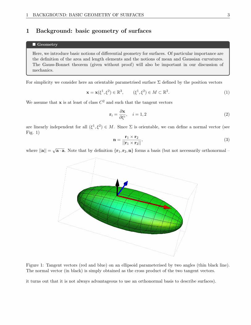
are linearly independent for all (ξ1, ξ2) ∈ M . Since Σ is orientable, we can define a normal vector (seeFig. 1)
n =r1 × r2
||r1 × r2||, (3)
where ||a|| =√a · a. Note that by definition {r1, r2,n} forms a basis (but not necessarily orthonormal –
Figure 1: Tangent vectors (red and blue) on an ellipsoid parameterised by two angles (thin black line).The normal vector (in black) is simply obtained as the cross product of the two tangent vectors.
it turns out that it is not always advantageous to use an orthonormal basis to describe surfaces).
1 BACKGROUND: BASIC GEOMETRY OF SURFACES 4
1.1 Length and area
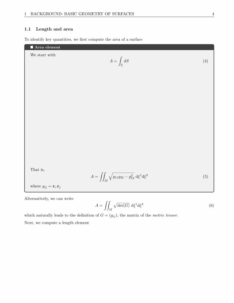
To identify key quantities, we first compute the area of a surface
� Area element
We start with
A =
∫ΣdS (4)
That is,
A =
∫∫M
√g11g22 − g212 dξ1dξ2 (5)
where gij = ri.rj
Alternatively, we can write
A =
∫∫M
√det(G) dξ1dξ2 (6)
which naturally leads to the definition of G = (gij), the matrix of the metric tensor.
Next, we compute a length element

1 BACKGROUND: BASIC GEOMETRY OF SURFACES 5
� Length element
We start with a curve r = r(t) defining a path γ on Σ
L =
∫γds (7)
That is,ds2 = gijdξ
idξj (8)
and
L =
∫I
√gij ξ̇iξ̇j dt (9)
Associated with the metric we have defined the first fundamental form ds2 = gijdξidξj .
1.2 Curvatures
We are interested in defining curvatures on the surface Σ. We consider a curve C on Σ passing througha point P and parameterised by its arc length s and define t as the tangent vector of C at P .
We know from Module 1 that the curvature of the curve C at a point P is obtained as |t′|. It is thereforenatural to define the curvature vector
k =dt
ds(10)
and decompose it into two components, the normal curvature vector kn and the geodesic curvature vectorkg
k = kn + kg (11)
where kn = −knn is along the normal vector1, that is
kn = −n · dtds
, kg = ||kg|| =∣∣∣∣t · (dt
ds× n
)∣∣∣∣ . (12)
The normal curvature kn is a property of the surface itself and gives the curvature in a planar slice spannedby the normal and tangent vector (see Fig. 1.2) whereas the geodesic curvature gives the curvature onthe curve on the surface (it is identically zero for a geodesic curve).
We can compute explicitly the normal curvature for a given curve.
1Note the choice of sign designed to ensure that the normal curvature of a sphere of radius R is indeed kn = +1/R ratherthan −1/R if we take n to be outer normal vector.

1 BACKGROUND: BASIC GEOMETRY OF SURFACES 6
Figure 2: The normal curvature of a curve on a surface in a given direction t is given by the curvatureof the curve obtained as the intersection of the surface with the plane spanned by n and t .
� The normal curvature
That is,kn = Kij(ξ
i)′(ξj)′ (13)
where
Kij = Kji = −n · ∂rj∂ξi
(14)
which naturally leads to the definition of K = (Kij), the matrix of the extrinsic curvature tensor. Thistensor is naturally associated with the second fundamental form Kijdξ
idξj .
A natural question is to determine the extremal values of the normal curvature as we vary the tangent

1 BACKGROUND: BASIC GEOMETRY OF SURFACES 7
vector at P .
� Principal curvatures
That is, the principal curvatures are the eigenvalues of the principal curvature matrix
L = G−1K. (15)
Define e1 and e2 as the orthonormal eigenvectors associated with the principal curvatures k1 and k2. Wecan write
t = cos θ e1 + sin θ e2 (16)
and, in general, we have (Euler’s theorem 1760, see Fig. 1.2)
kn = k1 cos2 θ + k2 sin
2 θ. (17)
The principal curvatures can be used to defined the mean curvature H and Gaussian curvature KG asfollows
2H = tr(L) = k1 + k2, (18)
KG = det(L) = k1k2. (19)
It can be shown that the Gaussian curvature is intrinsic to the surface (in the sense that it only dependson the metric and not on the normal vector). This result is contained in the Gauss’ famous TheoremaEgregium (remarkable theorem). Note that KG is independent of the parameterisation but that H canchange sign (depending on the choice of the normal vector).
A minimal surface is such that H = 0 identically for all points. These surfaces play a particularlyimportant role in a number of important problems and we will indeed see that the vanishing of the meancurvature naturally arises as a condition to minimise the area.
The Gaussian curvature is particularly important in the classification of surfaces as either elliptic (KG >0), hyperbolic (KG < 0), or parabolic (KG = 0).

1 BACKGROUND: BASIC GEOMETRY OF SURFACES 8
1k1
1k2
n
Figure 3: The principal curvatures of a surface are the maximal values of the normal curvature at a pointand geometrically correspond to the inverse radius of the best fitting circles (of maximal radii).
1.3 The Gauss-Bonnet theorem
An important result of global topology is the Gauss-Bonnet theorem (Bonnet 1848). Let Σ be a compacttwo-dimensional Riemannian manifold with boundary ∂Σ. Let KG be the Gaussian curvature of Σ, andkg the geodesic curvature of ∂Σ. Then∫
ΣKGdS +
∫∂Σ
kgds = 2πχ(Σ), (20)
where χ(Σ) is the Euler characteristic of Σ, a global topological property, which, for a surface of genus2
p is given by χ(Σ) = 2− 2p.
Of particular interest for us is the case of a closed orientable surface for which∫ΣKGdS = 4π(1− p). (21)
1.4 Examples
Examples of different minimal surfaces are given in Fig. 4. The corresponding Mathematica file thatcreated these graphs can be downloaded with the Lecture Notes material (“Curvature Computation.nb”).
2In three-dimensions, the genus of an orientable surface is given by the number of handles, a sphere has genus 0, a torusor a mug has genus 1, and so on.

1 BACKGROUND: BASIC GEOMETRY OF SURFACES 9
Figure 4: Different minimal surfaces. Left: the helicoid, Right: the catenoid. Middle: The helico-catenoid. Tangent vectors (red and blue). The normal vector (in black) is simply obtained as the crossproduct of the two tangent vectors.

2 FLUID BIOMEMBRANES 10
2 Fluid biomembranes
� Motivation
Many biological membranes are made of lipid bilayers and examples are given in MMB-Presentation, Bio-Membranes, online. Mechanically, these structures and synthetic lipid vesiclesresist bending, stretching but are fluid in the plane and as such do not resist shear. In this Chapterwe consider the model of Canham (1970)-Helfrich (1973)-Evans (1973) to describe the response ofsuch membranes under pressure.
2.1 The biomembrane model
We have the following assumptions:
A1. The biomembrane is thin enough with respect to its maximal radius of curvature and typical lengthso that it can be represented by a surface Σ.
A2. The biomembrane is shearless (offers no resistance to shear) but resists bending and stretching.
A3. The energy associated with change in bending is given by the lowest polynomial in the surface meanand Gaussian curvatures that preserve the parameterisation and the energy of stretching by thechange of area.
A pedantic but important remark: A membrane is a membrane but is not a membrane, in the sensethat the term membrane used in biology is the same term used by biophysicists but not the same as theterm “membrane” used in mechanics. In mechanics a membrane is a two-dimensional structure that canresist tension but not compression or bending. A plate is an initially flat structure that resists bending,tension, and compression (it can be unshearable or shearable depending on the theory). A shell is aninitially curved surface that resists bending, tension, and compression (it can be unshearable or shearabledepending on the theory). We will use the term biomembrane or fluid membrane to describe a shearlessstructure that can resist bending and stretching.
Following the assumptions, we posit that the elastic energy of a biomembrane with surface Σ is given by
E =
∫ΣdS
[γ + 2κ(H −H0)
2 + κ̄KG
](22)
where
• H and KG are the mean and Gaussian curvatures defined in the previous section,
• γ is the surface tension (as usually found in a theory of surfactant),
• κ is the bending modulus (confusing but standard notation),
• κ̄ is the saddle-splay modulus,
• H0 is the intrinsic mean curvature of the biomembrane.
In general, one can find the shape of the surface by minimising the energy E with respect to all continuousdeformations of a given reference shape. Typically, the system is subject to other constraints such as

2 FLUID BIOMEMBRANES 11
constant volume or constant pressure. In such cases, we can introduce the corresponding Lagrangemultiplier and minimise an amended function. For instance, for constant volume V = V0, the shape willbe obtained by minimising
EP = E − P (V − V0) (23)
subject to the condition V = V0. Here P is the Lagrange multiplier (which, of course can be identifiedas the pressure). Similarly for the case of constant pressure, we will need to minimise
EV = E − PV. (24)
Note that the set of extrema of EP and EV are the same but their stability will be in general different.
Remember that from the Gauss-Bonnet theorem for a closed surface, we have∫ΣKGdS = 4π(1− p). (25)
Therefore, for a closed surface the energy contribution of the Gaussian curvature during deformation isconstant (as long as the topology of the surface does not change) and can be ignored when determiningthe shape of the membrane.
Dimensionally, κ is an energy and γ is an energy per length squared. Therefore, we can define a typicallength scale of tension versus bending given by
λtb =
√κ
γ. (26)
� Estimates

2 FLUID BIOMEMBRANES 12
xc
yc
z
x
h(x,y)
y
Figure 5: The height function (or Monge parameterisation) of a surface. Note that this representation isnot valid if the surface curves back on itself (for instance in the case on the right).
2.2 The shape equation in the Monge representation
In order to find the shape of the surface we need to minimise the corresponding energy. This is in generala difficult task as the variations of the curvatures with respect to the deformation need to be found ingeneral. To illustrate this process, we consider here a simpler, but important, case where the surface Σcan be represented by a height function h = h(x, y) of class C2. That is,
h : U ∈ R2 → R, (∇h)2 < ∞, (27)
where ∇ = ex∂x + ey∂y. The position vector for points on the surface is simply
r = (x, y, h(x, y)) (28)
� Normal and metric
We first compute the normal and metric
So that, we have for example, n = g−1/2 (−∇h+ ez) , g = det(G) = 1 + (∇h)2.

2 FLUID BIOMEMBRANES 13
We can now compute the mean and Gaussian curvatures
� Curvatures in Monge representation
So that, we have2H = −g−3/2
[hxx(1 + h2y) + hyy(1 + h2x)− 2hxyhxhy
], (29)
andKG = g−2
(hxxhyy − h2xy
). (30)
The mean curvature can also be written in a coordinate free form as
2H = ∇ ·(g−1/2∇h
)= −∇ · n (31)
2.2.1 Area minimisation
Note that if κ = κ̄ = H0 = 0 and γ is constant, the energy for the biomembrane simplifies to thewell-known energy given in the theory of surface tension (in the absence of gravity)
ES = γ
∫ΣdS. (32)
We can now use Monge representation to obtain the condition for area minimisation

2 FLUID BIOMEMBRANES 14
� Condition for area minimisation
And we find the two equivalent local conditions for the existence of a minimal surface
∇.n = 0 ⇐⇒ H = 0. (33)
Note that this condition remains valid even in the general case (where a surface cannot be representedby a height function) but only provides necessary conditions.
2.2.2 Small gradient approximation
We further restrict our analysis to the case of κ̄ = H0 = 0 and for small gradients |(∇h)| ≪ 1.
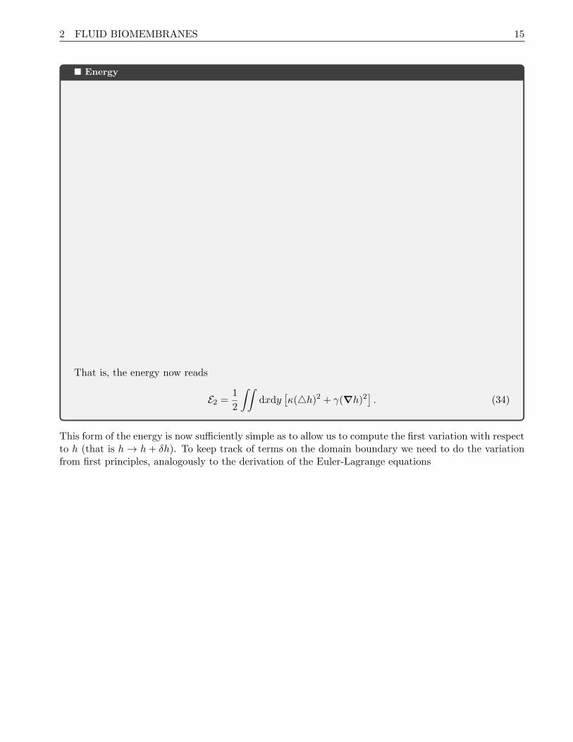
2 FLUID BIOMEMBRANES 15
� Energy
That is, the energy now reads
E2 =1
2
∫∫dxdy
[κ(△h)2 + γ(∇h)2
]. (34)
This form of the energy is now sufficiently simple as to allow us to compute the first variation with respectto h (that is h → h+ δh). To keep track of terms on the domain boundary we need to do the variationfrom first principles, analogously to the derivation of the Euler-Lagrange equations

2 FLUID BIOMEMBRANES 16
� First variation of the energy
That is, we have
δE2 =
∫∫dxdy△ [κ(△h)− γh] δh
+
∮ds N · [κ(△h)∇δh+ (γ∇h− κ∇△h)δh] . (35)
where N is the outer normal to the projected surface contour on the x− y plane.

2 FLUID BIOMEMBRANES 17
A necessary condition for minimisation is δE2 = 0. The vanishing of the area integral provides the shapeequation
△(△− λ−2
)h = 0 (36)
where λ = λtb is the typical length scale introduced in (26).
The vanishing of the line integral leads to boundary conditions for our fourth-order problem. We havetwo sets of conditions to satisfy.
1) For the first term in the bracket, we fix either the normal component of the contour so that
N ·∇h = Cst ⇒ N ·∇δh = 0 (37)
or, we impose △h = 0 on ∂Σ.
2) Similarly, we need to either fix h at the boundary so that δh = 0 at the boundary, or we impose
N ·∇h = λ−2N ·∇△h, (38)
for h on the boundary.
Together, this leads to four different possible sets of boundary conditions (or any combinations in differentparts of the domain).
2.3 Examples
2.3.1 One-dimensional fluid membranes
As a first particular case of the shape equation (36), we consider the case where h = h(x) only, that iswe assume that the sheet is uniform along the y axis. In this case, we have
∂4xh− λ−2∂2xh = 0, (39)
which is exactly the form of the beam equation in module 1, where λ−2 = F/(EI) plays the role of aneffective tension. We conclude that in the small gradient approximation and in one dimension, a uniformelastic fluid membrane behaves as an elastic beam under tension.
2.3.2 Flicker spectroscopy
A possible method to measure the elastic parameters of the membrane is provided by measuring thespectrum of thermal undulations via light microscopy [3, 5]. This is known as Flicker spectroscopy. Itis typically performed on closed membranes but the analysis of a square membrane will still provideinteresting information.
Consider a square membrane of size L× L with periodic boundary conditions. We expand the height ofthe membranes h(r) = h(x, y) as a double Fourier series:
h =∑q
hqeiq·r , q =
2π
L
(nx
ny
), nx, ny ∈ Z . (40)
Next, we compute the fluctuations of this membrane in thermal equilibrium.

2 FLUID BIOMEMBRANES 18
� Flicker Fluctuation
That is, we have ⟨|hq|2
⟩=
2kbT
L2(κq4 + σq2)(41)
The coefficients⟨|hq|2
⟩(known as the static structure factors) can be measured from the spectrum.
Fitting it to Eq. (41) yields the bending modulus and surface tension of the membrane (see Fig. 6).
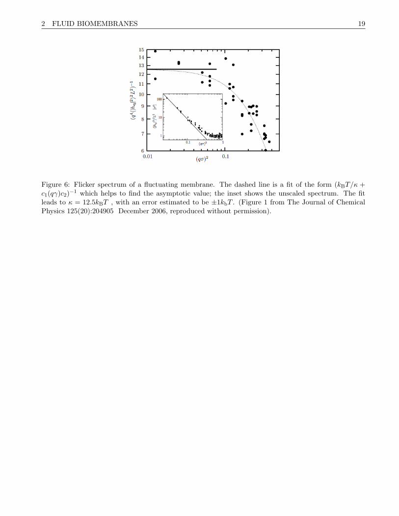
2 FLUID BIOMEMBRANES 19
Figure 6: Flicker spectrum of a fluctuating membrane. The dashed line is a fit of the form (kBT/κ +c1(qγ)c2)
−1 which helps to find the asymptotic value; the inset shows the unscaled spectrum. The fitleads to κ = 12.5kBT , with an error estimated to be ±1kbT . (Figure 1 from The Journal of ChemicalPhysics 125(20):204905 December 2006, reproduced without permission).

3 AXISYMMETRIC MEMBRANES AND SHELLS 20
3 Axisymmetric Membranes and Shells
� Elastic membranes and shells
We consider the axisymmetric deformation of membranes and shells in linear and nonlinearelasticity. These have biological application in modelling the dformation and mechanics of redblood cells in physiological flows and also modelling filamentous growth of biological structuresin the context of fungi and hyphae for instance. We start with a simple elastic membrane beforeconsidering the general case. Most of these notes follow the derivations from [8, 11, 6, 7], whichare motivated by in the context of filamentous growth.
3.1 Elastic membranes with linear constitutive laws
We begin by considering an extensible axisymmetric elastic membrane filled with an incompressibleviscous fluid under pressure and that there is no normal shear stress. This type of formulation has beenused successfully to describe the shape of red blood cells and other biomembranes [10, 9] and we adapt ithere to include the effects of pressure induced stretch, growth and geometry dependent elastic propertiesof the membrane. We assume that the shape of the membrane remains axisymmetric in the deformation.Here, to derive a full set of equations, we use a method based on rational mechanics, we proceed in threesteps: kinematics, mechanics, and constitutive laws.
3.1.1 Kinematics
θ(σ)
σ
(σ) r
s=s(σ)
s = σ=0
C
n
ntt
x
y
zφ
Figure 7: Basic membrane and shell geometry. A material point σ is measured by its arc-length, s(σ)from the apex of the shell and its axial position r(σ) on a curve C, n and t denotes the normal andtangent vectors at that point. The angle θ(s) is the angle between the normal direction. The membraneis taken to be axisymmetric where φ is the azimuthal angle.
We assume that the shape of the membrane remains axisymmetric in the deformation. As shown inFigure 7, the membrane surface S is defined by revolving a planar curve C around the z-axis. Thereference planar curve C is parameterized by a parameter σ counted from the intersection O of thesurface with the z-axis. The shell geometry is characterized by the distance from the axis r = r(σ) and

3 AXISYMMETRIC MEMBRANES AND SHELLS 21
the angle θ = θ(σ) between the normal to C at σ and the z-axis. The arclength at any time s = s(σ)is measured from O. Before deformation or growth, the material parameter σ is chosen to be the arclength, s = σ, and the initial shell configuration is referred to as the reference configuration. If weconsider axisymmetric deformation of the surface, we can define the radial stretch ratio
λφ =r
ρ, (42)
at a given (material) point as the ratio between the original radius ρ at that point and the new radius r,and the stretch ratio
r
ρr
Figure 8: Definitions of stretches. We consider a reference curve before and after deformation.
λs =∂s
∂σ, (43)
as the amount of stretching of the body coordinates with respect to arclength. These two stretches(λφ, λs) completely define the deformation of an axisymmetric reference shape. The geometric variablessatisfy the equations
dr
ds= cos(θ),
dz
ds= − sin(θ), (44)
Two other important measures of the geometry of the surface are the principal curvatures which aregiven by
κs =dθ
ds, κφ =
sin θ
r. (45)
Note 1: If the we have an incompressible shell the third deformation variable, λ3, measuring changes inthe normal thickness of the shell, is simply related to λs and λφ through the incompressibility conditionλsλφλ3 = 1.
Note 2: A modelling choice must be made at this point. Is the membrane, the reduction to a surfaceof a 3D body (as one would expect say of a rubber balloon), or is the membrane a true elastic surface(called “an elastic sheet”) with no transverse structure (as one would model a lipid bilayer)? This leadsto slightly different formulation of the problem. Haughton has a nice review paper on the subject [4].

3 AXISYMMETRIC MEMBRANES AND SHELLS 22
r(m)
x
y
z
s=m=0
Pressure difference P
tqeq
tses
Figure 9: The surface S with stresses (ts, tφ).
3.1.2 Mechanics
We now define the stresses acting on the membrane surface: let ts be the tension on the surface along thetangent es, in the direction of increasing arclength; and let tφ be the tension along the unit vector eφ,normal to es in a plane tangent to S, and in the direction of increasing azimuthal angle φ (see Figure 9).
The equations for mechanical equilibrium for a surface of revolution in the normal and tangential directionresults from the balance of force and moments acting on a surface element.

3 AXISYMMETRIC MEMBRANES AND SHELLS 23
� Mechanical force balance
That is, we have,
P = κsts + κφtφ, (46)
∂(rts)
∂s− tφ
∂r
∂s+ rf = 0, (47)
where P is the pressure difference across the membrane, and f is the shear stress on the membrane.
This last term could be taken to represent the drag forces exerted by the surrounding medium on themembrane. Appropriate modeling of this effect is nontrivial. For now, this term will be set to zero inour analysis.
We proceed to consider moments.

3 AXISYMMETRIC MEMBRANES AND SHELLS 24
� Mechanical moment balance
Hence
∂
∂s(rms)−mφ cos θ = 0. (48)
Note: The two equations (46, 47) can be written in terms of r and θ by using the geometric relationes = cos θer + sin θez, and ∂θ/∂s = κs, and take the form
ts∂θ
∂s+
sin θ
rtφ = P, (49)
∂ts∂s
=cos θ
r(tφ − ts). (50)
In the case of constant pressure P we can verify that there is an integral of equations (49, 50), i.e. afunction of the variables constant along the curve C, given by:
C = r2 (2tsκφ − P ) . (51)
In particular, for all solutions (r(σ), θ(σ)) crossing the z-axis, we have C = 0 and P = 2tsκφ.
3.1.3 Constitutive laws
In order to close the system of mechanical and geometric equations constitutive relations must beintroduced. These are developed through the introduction of an elastic free energy function for thethree-dimensional material, specified as energy per unit volume,
W = W (I1, I2, I3) (52)

3 AXISYMMETRIC MEMBRANES AND SHELLS 25
where I1, I2, I3 are the strain invariants
I1 = λ2s + λ2
φ + λ23, (53)
I2 = λ2sλ
2φ + λ2
sλ23 + λ2
φλ23, (54)
I3 = (λsλφλ3)2 (55)
Here λ3 = h/H is the strain associated with the change in thickness from the original H to the current h.The incompressibility condition implies that both λ3 = 1/λsλφ and all derivatives of W can be expressedin terms of I1 and I2.
We recall that from the general theory of elasticity for isotropic incompressible material, we have
ti = λi∂W
∂λi− p, i = s, φ, 3. (56)
From this three-dimensional theory, we seek constitutive relationship for our two-dimensional membraneusing both incompressibility and the membrane assumption that states t3 = 0.
� Constitutive law
One concludes that the stresses are given by the relations
ts = 2Hλ3(λ2s − λ2
3)
(∂W
∂I1+ λ2
φ
∂W
∂I2
)−Hλ3W, (57)
tφ = 2Hλ3(λ2φ − λ2
3)
(∂W
∂I1+ λ2
s
∂W
∂I2
)−Hλ3W. (58)
In these relations H is the undeformed shell thickness, and the factor Hλ3 represents the change in wallthickness in the current (i.e. stressed) configuration. We comment that the thickness pre-factor means

3 AXISYMMETRIC MEMBRANES AND SHELLS 26
that the ts and tϕ have units of force per unit length, i.e. they have the dimensions of tensions ratherthan stresses. Using these formulae we note that
ts − tφ = 2Hλ3(λ2s − λ2
φ)
(∂W
∂I1+ λ2
3
∂W
∂I2
). (59)
The choice of W depends on the problem at hand. A popular choice for elastomers is the Mooney-Rivlinmodel
W = C1(I1 − 3) + C2(I2 − 3), (60)
where C1 and C2 are certain elastic parameters. When C2 = 0 (60) reduces to the so called neo-Hookeanmodel, and for small deformations C1 is related to Young’s modulus, E, by E = 6C1. We note thatdespite its linearity in the invariants the Mooney-Rivlin potential, and its neo-Hookean limit, are stillcapable of describing finite deformations and becomes highly nonlinear in the final equations due to thetransformation from reference to current configuration. A variety of nonlinear material responses can becaptured by considering more other functional forms of W , e.g. for soft tissue the Fung energy
W =C1
γ
(eγ(I1−3) − 1
)(61)
is often used which for small γ reduces to the neo-Hookean model. Given any model, we write theconstitutive relationships (57,58) in the form
ts = Afs(λs, λφ), (62)
tφ = Afφ(λs, λφ), (63)
where fs, fϕ are dimensionless functions and A provides the dimensional factor appropriate for the scalingof the equilibrium equations. For the neo-Hookean and Mooney-Rivlin energies A = 2C1h.
For small deformations the neo-Hookean model gives constitutive relations similar to those of standardlinear elasticity theory and it is sometimes convenient to refer (albeit imprecisely) to these relations as“linear”.
Moments. Finally, we need to specify a constitutive relationship for the bending moments. The bendingmoments are assumed to be isotropic and proportional to the change in the surface’s mean curvature,i.e.
mφ = ms = B(κs + κφ −K0), (64)
where K0 K0 is the sum of membrane curvtaures in the absence of bending moments and B is the bendingmodulus [E. A. Evans and R. Skalak. Mechanics and thermodynamics of biomembranes. CRC Press,Inc, Boca Raton, Florida, 1980].
Combining this with equation (48) immediately implies
κs + κφ = K1,
where K1 is a constant.
In summary To find the membrane shape, that is r, z, with constant pressure the complete system of

3 AXISYMMETRIC MEMBRANES AND SHELLS 27
membrane equations can be written as the closed system
ds
dσ= λs, (65)
dz
dσ= −λs sin(θ), (66)
dr
dσ= λs cos(θ), (67)
dθ
dσ= λsκs = λs
(K1 −
sin θ
r
), (68)
dtsdσ
= λsA
[cos θ
r(fφ − fs)
]. (69)
with fs = fs(λs,rρ), fφ = fφ(λs,
rρ), with initial profile z = z0(s), r = ρ(s), from which initial curvatures
and thus K1 can be found.
Note 1: computationally, this is a BVP for 4 unknowns r, z, θ, s. It can easily be solved numerically.Some care is needed to find the correct boundary value at σ = 0 It can also be solved asymptoctically forsimple configurations.
Note 2: If volume rather than pressure is kept constant, then the pressure becomes a Lagrange multiplierthat enforces the volume constraint. Starting from a guess pressure, one can iterate the computation bycomputing the solution for each pressure under a volume constraint).
Note 3: In the case of a surface incompressibility (typical for bilayers), one needs to modify the strainenergy density with the constraint, the associated new “‘surface pressure” will then need to be determinedas part of the unknowns. This is a possible way to relate this theory to the fluid membranes section above.
3.1.3.1 Variable moduli. A deformation of the membrane can follow from either an increase inpressure or a softening of the walls. The softening can easily be taken into account by using a materialdependent elastic function A = A(σ). A general form of p = P/A can be taken as
p =P
2
[1− tanh(
σ − σ1α
)
]+ β, (70)
where P is the internal pressure and the parameters σ1 and α describe the length of the extension zone.Since limσ→∞ p = β, the parameter β describes the effective pressure in distal regions. Close to thedeformation tip (σ = 0), the walls are soft and the elastic coefficient minimal. In the distal regions,the walls are set and the elastic coefficient A is, comparatively, very large, so that the effective pressureis small (equal to β). Note that a decreased modulus or increased pressure (or vice versa) are, at themechanical level, indistinguishable, trivial mathematically, highly non-trivial biologically.
3.1.4 Inflation of a spherical membrane
It is of interest to consider the inflation of a spherical membrane.
3 AXISYMMETRIC MEMBRANES AND SHELLS 28
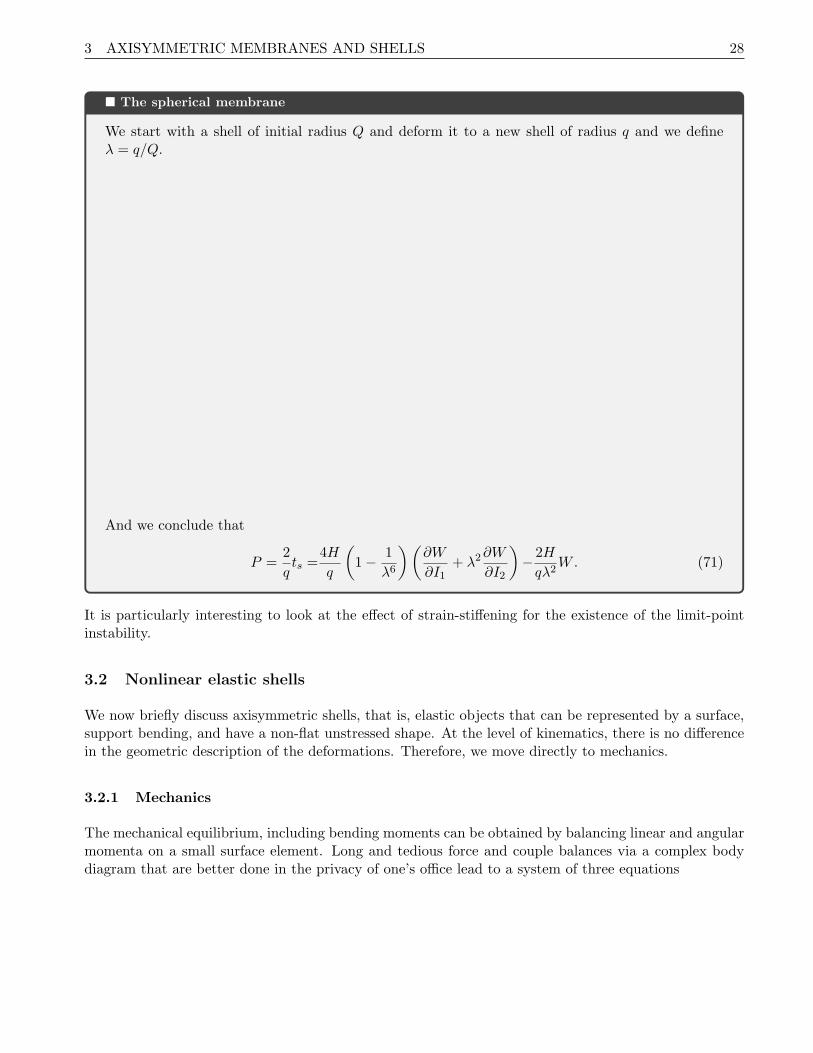
� The spherical membrane
We start with a shell of initial radius Q and deform it to a new shell of radius q and we defineλ = q/Q.
And we conclude that
P =2
qts =
4H
q
(1− 1
λ6
)(∂W
∂I1+ λ2∂W
∂I2
)− 2H
qλ2W. (71)
It is particularly interesting to look at the effect of strain-stiffening for the existence of the limit-pointinstability.
3.2 Nonlinear elastic shells
We now briefly discuss axisymmetric shells, that is, elastic objects that can be represented by a surface,support bending, and have a non-flat unstressed shape. At the level of kinematics, there is no differencein the geometric description of the deformations. Therefore, we move directly to mechanics.
3.2.1 Mechanics
The mechanical equilibrium, including bending moments can be obtained by balancing linear and angularmomenta on a small surface element. Long and tedious force and couple balances via a complex bodydiagram that are better done in the privacy of one’s office lead to a system of three equations

3 AXISYMMETRIC MEMBRANES AND SHELLS 29
r r
Figure 10: A rather complex balance of forces and moments acting on a surface element, where thedifference in the normal stress across the membrane is qn, which has a pressure contribution, but mayhave other contributions as well, as detailed further in the text.
d(rqs)
ds= rqn − r (κsts + κφtφ) , (72)
d(rts)
ds= tφ cos θ + rκsqs, (73)
d(rms)
ds= mφ cos θ + rqs, (74)
where ts and tφ are, respectively, the meridional and azimuthal stresses; ms and mφ are the bendingmoments; and qs is the shear stress normal to the surface.
In equation (72), which represents the balance of normal stresses, qn represents the total normal stressexerted on the shell. If the problem is pressure driven then qn = ∆P , namely the pressure differenceacross the shell; and if it is a combination of pressure and cytoskeletal action, represented by somefunction τn, then qn = ∆P + τn.
Note: If the normal forces acting on the shell are due to, say, cytoskeletal action represented by somefunction τn, then qn = τn; and if the total normal forces are a combination of both of these effects,qn = ∆P + τn.
In Equation (73), which represents the balance of tangential stresses, τs is the external tangential shearstress acting on the shell and will be used here to represent the friction between the deformed shell andits environment.
3 AXISYMMETRIC MEMBRANES AND SHELLS 30
3.2.2 Constitutive relationship
For the stresses ts, tφ, we use the same relationships as for the case of membranes (57-58). Finally, weneed to specify a constitutive relationship for the bending moments. Similarly for the moments we useas previously
mφ = ms = B(κs + κφ −K0), (75)
where B is the bending modulus and K0 is the sum of membrane curvatures in the absence of bendingmoments.
3.2.3 The shell equations
The geometric and mechanical equations can be combined to give a closed system. It is convenient toexpress all the derivatives in terms of the material coordinate, σ, leading to
dz
dσ= −λs sin(θ), (76)
dr
dσ= λs cos(θ), (77)
dθ
dσ= λsκs, (78)
dκsdσ
= λs
[cos θ
r
(sin θ
r− κs
)+
qsB
](79)
dtsds
= λsA
[cos θ
r(fφ − fs) + κs
qsA
], (80)
dqsdσ
= λsA
[qnA
− κsfs −sin θ
rfφ − qs
A
cos θ
r
], (81)
where (79) is obtained from (74) using the constitutive relation (75) and equation (45) is used to expressκφ in terms of r and θ. In equations (80) and (81) ts and tφ are expressed in terms of λs and λφ throughthe scaled constitutive relations (62,63), and equation (80) is converted into a differential equation for λs
by eliminating λφ through the relation λφ = r/ρ.
The six ordinary differential equations (76-81) together with the relationships (62,63) and λφ = r/ρform a closed system for the variables (z, r, θ, κs, λs, qs) that can be solved for given initial profile ρ(σ),elastic parameters A,B, prescribed normal and tangential stresses qn and τn, and appropriate boundaryconditions.
When bending moments can be neglected the shell no longer supports an out-of-plane shear force, i.e.qs = 0 and equation (81) reduces to
qnA
= κsfs + κφfφ, (82)
which is just a generalized form of the Young-Laplace law as seen before. The system of shell equations

3 AXISYMMETRIC MEMBRANES AND SHELLS 31
Organisms w h P E ξ G Ref
A. nidulans mature 3 46 1.4 115 0.8 0.2-0.5 Ma et al. (’05)
A. nidulans tip 3 46 1.4 75 1.2 0.2-0.5 Ma et al. (’05)
M. gryphiswaldenese 0.5 1 0.1 30 0.003 Arnoldi (’00)
Table 1: w: width (µm), h: thickness (mm), P : Pressure (MPa), G: growth rate (µm/min), E: Young’smodulus (MPa)
then simplifies to the membrane equations from the previous section.
ds
dσ= λs, (83)
dz
dσ= −λs sin(θ), (84)
dr
dσ= λs cos(θ), (85)
dθ
dσ= λsκs = λs
(K1 −
sin θ
r
)(86)
dtsdσ
= λsA
[cos θ
r(fφ − fs)
]. (87)
3.3 Scalings
It is useful to introduce the following dimensionless number for the problem
ξ =Peffw
3A(88)
where w is a characteristic macroscopic length scale (typically, the width of the tip, or the radius of acell), Peff is a measure of the normal force per unit area acting on the walls and A characterizes thewall elastic properties. The number ξ gives a measure of the magnitude of the deformation, i.e. shellsunder different normal loads and with different elastic properties will experience the same magnitude ofdeformation from their initial unstressed state as measured in terms of their tip widths. That is, highvalues of ξ representing either a soft material or a high pressure result in large elastic deformations,whereas low values of ξ corresponding to either a rigid material or low pressure result in small elasticdeformations. For a neo-Hookean material we can relate A to the Young’s modulus E = 3A/h, where his the thickness of the shell or membrane, so that
ξ =Peffw
hE. (89)
Detailed studies of mechanical behaviour of microorganisms are difficult and only a few estimates havebeen proposed (See Table 7).
To set the scales an estimates of the elastic and bending modulii is required. An order of magnitudeestimate can be obtained from the Young-Laplace law for a spherical membrane under pressure; namelythe relationship between the pressure difference ∆P across the membrane wall, the sphere radius R, andthe membrane stresses, which we express in the form
∆P =h(σθθ + σϕϕ)
R(90)

3 AXISYMMETRIC MEMBRANES AND SHELLS 32
where h is the membrane thickness and σθθ, σϕϕ are, respectively, the meridional (longitudinal) andazimuthal (hoop) stresses3. Because of the spherical symmetry σθθ = σϕϕ. To a first approximation thesestresses scale as σ ∼ E, where E is the membrane’s elastic modulus. As an example, if the typical radiusis of order 3µm, and the pressure is about ∆P ∼ 1 − 8MPa with a wall thickness of h ∼ 0.1µm, theYoung’s modulus E is of the order of magnitude
E ∼ 10− 100MPa,
which is consistent with that of many other biological materials shown in the elastic moduli atlases ofAshby et. al. [1]. We also note that this estimate is based on a linear constitutive relationship, so in thecontext of fungal hypahe tips, if the radius of the appressorium stays approximately constant under anincrease in turgor pressure, the corresponding estimate of the elastic modulus increases proportionately.Thus, if the turgor pressure increases five-fold and the radius is, to a first approximation, unchanged, theelastic modulus (which is really the local slope of the stress/strain plot) of the wall could be considered tohave increased five-fold. In this sense the wall could be considered a “smart material”; namely adjustingits properties in response to a change in its local environment.
Elastic shell theory (e.g. L. D. Landau and E. M. Lifshitz. Theory of elasticity. Pergamaon Press, 1959)also tells us that the bending modulus for a thin sheet is given, in the framework of linear elasticitytheory, by the relation B = Eh3/
(12(1− ν2)
), where ν is the Poisson ratio. Although not typically
known for many cellular walls, we can assume ν = 1/2, i.e. an incompressible material. This leads tothe estimate
B ∼ 10− 100× 10−13N m.
Clearly bending effects will only be significant if the cell wall exhibits regions of very high curvature.These types of estimates for E and B have been used by Boudaoud [2] to analyze morphological scalinglaws for the study of the mechanics of a large class of microorganisms, and used to distinguish familiesthat are tension dominated (where E is the significant parameter) and bending dominated (where B isthe significant parameter).
3Here we recall that stress is defined as force per unit area and tension as force per unit length. Thus for a bubbleequation (90) can be written as the familiar Young-Laplace equation ∆P = 2T/R where T is the surface tension (force perunit length).

4 PROBLEMS 33
4 Problems
Problems marked with a star* are meant to challenge you beyond the regular course. It is up to you to decide if
you want to try them. You will not be marked down for not answering them or for any mistake. I suggest that
you give them a try and think about these problems as a way to gain a deeper understanding of the material.
1) Show that the definitions of area (Eq. (6)) and length (Eq. (9)) are invariant under a change ofparameterisation.
2) The matrices G and K associated with the first and second fundamental form are symmetric.However, the combination L = G−1K is not necessarily symmetric. Prove that, nevertheless, theeigenvalues of L are real and one can always find an orthonormal set of eigenvectors that diagonalisesL.
3) Prove Euler’s theorem given in Eq. (17).
4) Draw and compute all the curvatures (principal, mean, Gaussian) for the monkey-saddle definedby z = x3 − 3xy2. Show that every point has negative Gaussian curvature, except the origin.
5) The Enneper-Weierstrass parameterization of a minimal surface is given by two complex functionf(z) and g(z) such that
x = ℜ(∫
f(1− g2)dz
)(91)
y = ℜ(∫
if(1 + g2)dz
)(92)
x = ℜ(∫
2fgdz
)(93)
Use this parameterisation to draw and compute the curvatures of the Enneper surface (f = 1, g(z) =z) and the Sherk surface (f = 4(1− z2), g(z) = iz). (Hint: use z = r exp(iθ) so that (r, θ) are theparameters for the surface).
6) Compute the mean and Gaussian curvatures of a slightly deformed sphere. That is, find to orderO(ϵ), the curvatures of
x(θ, ϕ) = R(1 + ϵh(θ, ϕ)) [cos(ϕ) sin(θ), sin(ϕ) sin(θ), cos(θ)] (94)
and show that they can be expressed as
H =tr(L)
2=
1
R
(1− ϵ
2∆(θ, ϕ)
)+O(ϵ2) (95)
K = det(L) =1
R2(1− ϵ∆(θ, ϕ)) +O(ϵ2). (96)
where
∆ = 2h+1
sin2 θ∂ϕϕh+ cot θ ∂θh+ ∂θθh. (97)
7) Show the equivalence between the two formulations of the mean curvature in the Monge represen-tation given by Eqs.(29) and (31).

4 PROBLEMS 34
8) Show that the addition of the constraint of fixed volume or fixed pressure adds a constant P termto the shape equation (36), so that it reads now
△(△− λ−2
)h = P. (98)
Hint: you may want to rewrite the volume integral∫dV as 1/3
∫∇ · r dV so that you can use the
divergence theorem to transform it into a surface integral.
9) Compute the shape of a membrane that smoothly covers a step-edge of height h0 and touches thelower level a distance L away (see Fig. 11). Assume that the height only depends on x.
Figure 11: Find the shape of a fluid membrane attached at height h0.
10) Consider a family of cylindrical vesicles of unstressed radius R0, current radius R, and length Lunder constant pressure P . Ignoring all boundary conditions at the face of the cylinder, computethe pressure P = P (R) and surface tension γ = γ(R) necessary to maintain this cylindrical shape byminimising the energy (24) with respect to both R and L (assume κ = 1 without loss of generality).Plot P as a function of R and find the maximal value of the pressure and the radius at which itoccurs. Discuss this profile and the possibility of an instability.
11) Plot the pressure versus radius curve for the Fung potential (61) and find the value of γ such thatthe limit-point instability disappears (that is for which the function P = P (a) ceases to have amaximum.)

REFERENCES 35
References
[1] MF ASHBY, LJ GIBSON, U WEGST, and R OLIVE. THE MECHANICAL-PROPERTIES OFNATURAL MATERIALS .1. MATERIAL PROPERTY CHARTS. PROCEEDINGS OF THEROYAL SOCIETY-MATHEMATICAL AND PHYSICAL SCIENCES, 450(1938):123–140, 1995.
[2] A Boudaoud. Growth of walled cells: From shells to vesicles. PHYSICAL REVIEW LETTERS,91(1), 2003.
[3] F. Brochard and J. F. Lennon. Frequency spektrum of flicker phenomenon in erythrocytes. J.Phys.–Paris, 36(11): pp. 1035–1047, 1975.
[4] Haughton DM. Elastic Membranes. In NonLinear Elasticity, London Mathematical Society LectureNote Series, Eds. Fu YB and Ogden RW, pages 233–67, ISBN–13: 9780511893698, 2001.
[5] J. F. Faucon, M. D. Mitov, P. Meleard, I. Bivas, and P. Bothorel. Bending elasticity and thermalfluctuations of lipid-membranes– theoretical and experimental requirements. J. Phys.–Paris, 50(17):pp. 2389–2414, September 1989.
[6] A Goriely, G Karolyi, and M Tabor. Growth induced curve dynamics for filamentary micro-organisms. JOURNAL OF MATHEMATICAL BIOLOGY, 51(3):355–366, 2005.
[7] A Goriely and M Tabor. Biomechanical models of hyphal growth in actinomycetes. JOURNAL OFTHEORETICAL BIOLOGY, 222(2):211–218, 2003.
[8] Alain Goriely and Michael Tabor. Estimates of biomechanical forces in Magnaporthe grisea.MYCOLOGICAL RESEARCH, 110(7):755–759, 2006.
[9] TW SECOMB and JF GROSS. FLOW OF RED-BLOOD-CELLS IN NARROW CAPILLARIES -ROLE OF MEMBRANE TENSION. INTERNATIONAL JOURNAL OF MICROCIRCULATION-CLINICAL AND EXPERIMENTAL, 2(3):229–240, 1983.
[10] R SKALAK, A TOZEREN, RP ZARDA, and S CHIEN. STRAIN ENERGY FUNCTION OF REDBLOOD-CELL MEMBRANES. BIOPHYSICAL JOURNAL, 13(3):245–280, 1973.
[11] Anthony Tongen, Alain Goriely, and Michael Tabor. Biomechanical model for appressorial designin Magnaporthe grisea. JOURNAL OF THEORETICAL BIOLOGY, 240(1):1–8, 2006.