mathematical methods inquantum chemistrychristian.mendl.net/science/publications/oberwolfach...scale...
TRANSCRIPT

Mathematisches Forschungsinstitut Oberwolfach
Report No. 32/2011
DOI: 10.4171/OWR/2011/32
Mathematical Methods in Quantum Chemistry
Organised byGero Friesecke, Munchen
Peter Gill, Canberra
June 26th – July 2nd, 2011
Abstract. The field of quantum chemistry is concerned with the analysisand simulation of chemical phenomena on the basis of the fundamental equa-tions of quantum mechanics. Since the ‘exact’ electronic Schrodinger equationfor a molecule with N electrons is a partial differential equation in 3N di-mension, direct discretization of each coordinate direction into K gridpointsyields K3N gridpoints. Thus a single Carbon atom (N = 6) on a coarse tenpoint grid in each direction (K = 10) already has a prohibitive 1018 degreesof freedom. Hence quantum chemical simulations require highly sophisticatedmodel-reduction, approximation, and simulation techniques.
The workshop brought together quantum chemists and the emerging andfast growing community of mathematicians working in the area, to assessrecent advances and discuss long term prospects regarding the overarchingchallenges of(1) developing accurate reduced models at moderate computational cost,(2) developing more systematic ways to understand and exploit the multi-
scale nature of quantum chemistry problems.Topics of the workshop included:
• wave function based electronic structure methods,• density functional theory, and• quantum molecular dynamics.
Within these central and well established areas of quantum chemistry, theworkshop focused on recent conceptual ideas and (where available) emergingmathematical results.
Mathematics Subject Classification (2000): 81Q05 (81V55, 65Y20).

1770 Oberwolfach Report 32/2011
Introduction by the Organisers
The field of quantum chemistry is concerned with the analysis and simulation ofchemical phenomena on the basis of the fundamental equations of quantum me-chanics. While mathematical thinking (by physicists and chemists) has alwaysplayed a large role in this field, in the past years a growing and very active com-munity of mathematicians working in the area has also emerged. The workshopwas interdisciplinary, bringing together quantum chemists and mathematiciansto assess the state of the art and discuss recent conceptual ideas and emergingmathematical results.
The Oberwolfach institute and format (of fewer talks than standard conferences)provided an ideal venue. It stimulated not just lively discussions (by no meanslimited to the explicit 10-minutes discussion slot allocated after each morninglecture). The Oberwolfach format also proved a fertile ground for cultural cross-fertilization. A clear proof that the latter was taking place was that by Wednesdaymorning, the first quantum chemist (Alexander Auer) was ready to spontaneouslygive up his planned laptop presentation for a blackboard talk.
Recurring themes of the meeting were (1) the continuing search for accuratecomputational methods with feasible computational cost, (2) the need for de-veloping more systematic ways to understand and exploit the multiscale natureof quantum chemical systems, (3) new examples of quasi-exactly soluble many-electron systems.
As regards theme (1), the ‘exact’ electronic Schrodinger equation for an atomor molecule with N electrons is a partial differential equation in 3N dimensions,so direct discretization of each coordinate direction into K gridpoints yields K3N
gridpoints; thus the unreduced equation for a single Carbon atom (N = 6) on acoarse ten point grid in each direction (K = 10) already has a prohibitive 1018
degrees of freedom. The computational cost of the best wave function based meth-ods, such as multiply-excited Configuration-Interaction methods or Coupled Clus-ter theory, while no longer exponential, still scales like an unphysically steep powerof the particle number. By contrast, density functional theory, which replaces thelinear many-electron Schrodinger equation in 3N dimensions by a nonlinear sys-tem of partial differential equations in 3 dimensions, is applicable up to thousandsof atoms (and hence the method of choice in most applications in materials sci-ence, molecular biology, and nanotechnology), but its modelling approximationshave proven hard to systematically understand or improve despite great effort overmany years.
Recent ideas to directly attack the curse of dimensionality of electronic wave-functions which were presented at the workshop included: the derivation and im-plementation of symmetry-projected Hartree-Fock-Bogoliubov theory for molecu-lar electronic structure problems (talk by Gustavo Scuseria); design of a stochastic‘game’ of life, death and annihilation in Slater determinant space (talks by AliAlavi and Alex Thom); the recently developed general mathematical format oftruncation and low-rank approximation of tensors (talk by Wolfgang Hackbusch);quantum-chemical versions of the density matrix renormalization group algorithm

Mathematical Methods in Quantum Chemistry 1771
and its analysis in the context of the matrix product state alias TT tensor for-mat (talk by Reinhold Schneider); the recent proof of high mixed regularity ofSchrodinger electronic wavefunctions and its implications for efficient approxima-bility in sparse bases (talk by Harry Yserentant); a sophisticated combination ofcoupled-cluster theory and low-rank approximation of tensors (talk by AlexanderAuer); use of a Jastrow ansatz with prefactor optimization via a quantum MonteCarlo approach (talk by Heinz-Jurgen Flad), efficient iterative symmetry decom-position for large atoms (talk by Christian Mendl); hierarchical decompositionof total molecular energies into contributions from different bond orders (Fred-erik Heber); and use of a Smolyak grid and an efficient quadrature scheme builtfrom nested 1D quadratures to solve the vibrational Schrodinger equation (talk byTucker Carrington).
Another important aspect in computational cost reduction is the structure of theunderlying single-particle basis sets. Werner Kutzelnigg presented sophisticatedresults on completeness and convergence rates for Gaussian and exponential bases,Lin Lin presented novel adaptive local basis sets for efficient density functionaltheory calculations in solids, and Peter Pulay gave a quantum chemist’s view onbasis sets based on his own more than 40 years of work in the area.
Volker Bach gave an overview over old and new mathematical results in Hartree-Fock theory, Thomas Oestergaard Soerensen explained his recent work on localanalyticity of Schrodinger wavefunctions in the interparticle positions and dis-tances, and Thorsten Rohwedder and Saber Trabelsi presented rigorous analyses ofthe coupled cluster equations respectively the multi-configuration time-dependentHartree-Fock equations. Heinz Siedentop derived and analyzed a mathematicalmodel for interacting Dirac Fermions in graphene quantum dots.
Progress related to multiscale aspects of many-electron systems included thederivation, analysis and implementation of a governing equation for the distor-tion in electronic structure caused by a defects in a solid (opening talk by EricCances). Note that in an approximating N -particle system the total energy isorder N , but the desired energy contribution is order 1, and one needs to passto the limit N → ∞. Similar scale issues (with small parameter being the re-ciprocal of the number of particles) appear when one is interested in the energyrequired to perturb the density of a Fermi gas (talk by Mathieu Lewin) and thedistortion of electronic structure in a solid by elastic deformation (talk by Jian-feng Lu). Another important small parameter appears in quantum moleculardynamics, namely the ratio between electronic and nuclear mass; this parameteris traditionally exploited both by adiabatic decoupling of electronic and nuclearmotion (Born-Oppenheimer approximation) and semiclassical approximation ofthe nuclear motion. Subtle ways of exploiting this smallness even when the tra-ditional assumptions of the Born-Oppenheimer approximation (namely uniformgaps between electronic energy levels) are violated were presented by CarolineLasser (numerical approximations of quantum molecular dynamics) and VolkerBetz (asymptotic analysis of quantum dynamics at avoided crossings of electronic

1772 Oberwolfach Report 32/2011
levels). George Hagedorn explained his recent derivation and analysis (and ensu-ing predictions) of non-classical Born-Oppenheimer-type approximations for thevibrational Schrodinger equation for hydrogen-bonded systems; here one exploitsthe smallness of the mass of the hydrogen nucleus compared to the other nuclearmasses.
New examples of quasi-exactly soluble many-electron models were presented byJerzy Cioslowski (electrons in spherical confining potentials), Pierre-Francois Loos(electrons restricted to hyperspheres), and Ben Goddard (highly charged atomicions).
Another highlight of the workshop was a very well attended Thursday eveningsession with short presentations by the graduate students Virginie Ehrlacher,Robert Lang, Stefan Kuhn, Andre Uschmajew, Fabian Hantsch, and Stefan Hand-schuh, which – just like the daytime lectures – were followed by lively discussion.

Mathematical Methods in Quantum Chemistry 1773
Workshop: Mathematical Methods in Quantum Chemistry
Table of Contents
Werner KutzelniggRate of convergence of basis expansions in Quantum Chemistry . . . . . . . 1775
Jerzy CioslowskiElectrons in Spherical Confining Potentials . . . . . . . . . . . . . . . . . . . . . . . . . 1785
Eric Cances (joint with A. Deleurence, V. Ehrlacher, M. Lewin)Local defects in quantum crystals . . . . . . . . . . . . . . . . . . . . . . . . . . . . . . . . . . 1787
Mathieu Lewin (joint with Rupert L. Frank, Elliott H. Lieb and RobertSeiringer)How Much Energy Does it Cost to Make a Hole in the Fermi Sea? . . . . 1790
Lin Lin (joint with Weinan E, Jianfeng Lu and Lexing Ying)Towards the optimal basis set in Kohn-Sham density functional theory . 1793
George A. Hagedorn (joint with Alain Joye)A Modified Born–Oppenheimer Approximation for Hydrogen Bonding . . 1795
Wolfgang HackbuschNumerical Tensor Calculus . . . . . . . . . . . . . . . . . . . . . . . . . . . . . . . . . . . . . . . 1798
Harry YserentantOn the mixed regularity of electronic wavefunctions . . . . . . . . . . . . . . . . . . 1801
Andre UschmajewThe regularity of tensor product approximations in L2 in dependence ofthe target function . . . . . . . . . . . . . . . . . . . . . . . . . . . . . . . . . . . . . . . . . . . . . . . 1802
Frederik Heber (joint with Michael Griebel, Jan Hamaekers)BOSSANOVA - A bond order dissection approach for efficient electronicstructure calculations . . . . . . . . . . . . . . . . . . . . . . . . . . . . . . . . . . . . . . . . . . . . 1804
Alexander A. Auer (joint with Udo Benedikt, Mike Espig, WolfgangHackbusch)Tensor Decomposition in Electronic Structure Theory: Canonical ProductFormat and Coupled Cluster Theory . . . . . . . . . . . . . . . . . . . . . . . . . . . . . . . 1808
Thorsten RohwedderA numerical analysis for the Coupled Cluster equations . . . . . . . . . . . . . . . 1812
Heinz-Jurgen Flad (joint with Sambasiva Rao Chinnamsetty, HongjunLuo, Andre Uschmajew)Bridging the gap between quantum Monte Carlo and explicitly correlatedmethods . . . . . . . . . . . . . . . . . . . . . . . . . . . . . . . . . . . . . . . . . . . . . . . . . . . . . . . . 1815

1774 Oberwolfach Report 32/2011
Heinz Siedentop (joint with Reinhold Egger, Alessandro De Martino, andEdgardo Stockmeyer)Multiparticle equations for interacting Dirac Fermions in graphenenanostructures . . . . . . . . . . . . . . . . . . . . . . . . . . . . . . . . . . . . . . . . . . . . . . . . . . 1819
Benjamin D. Goddard (joint with Gero Friesecke)Atomic Structure via Highly Charged Ions . . . . . . . . . . . . . . . . . . . . . . . . . . 1820
Christian B. Mendl (joint with Gero Friesecke)Electronic Structure of 3d Transition Metal Atoms . . . . . . . . . . . . . . . . . . . 1822
Alexander James William ThomStochastic Coupled Cluster Theory . . . . . . . . . . . . . . . . . . . . . . . . . . . . . . . . . 1824
Robert Lang (joint with Gero Friesecke)Relativistic effects in highly charged ions . . . . . . . . . . . . . . . . . . . . . . . . . . . 1827
Tucker Carrington Jr. (joint with Gustavo Avila)Using sparse grids to solve the vibrational Schrodinger equation . . . . . . . 1829
Fabian Hantsch (joint with Marcel Griesemer)Unique Hartree-Fock Minimizers for Closed Shell Atoms . . . . . . . . . . . . . . 1834
Reinhold SchneiderQC-DMRG and recent advances in tensor product approximation . . . . . . 1835
Gustavo E. Scuseria (joint with Carlos A. Jimenez-Hoyos, Thomas M.Henderson, Kousik Samanta, Jason K. Ellis)Projected quasiparticle theory for molecular electronic structure . . . . . . . . 1838

Mathematical Methods in Quantum Chemistry 1775
Abstracts
Rate of convergence of basis expansions in Quantum Chemistry
Werner Kutzelnigg
1. Basis expansions. General
The simplest kind of a basis expansion is that of a generalized Fourier expan-
sion. One expands a function f(x) in an orthonormal basis χ(n)p that becomes
complete (with an appropriate meaning) for n→∞
(1) f(x) = limn→∞
fn(x); fn(x) =n∑
p=1
c(n)p χ(n)p
This converges exponentially, in a Hilbert space norm, if f(x) is differentiable aninfinite number of times. Otherwise the convergence obeys an inverse-power lawwith a power depending on the differentiability of f(x). Such a rate of convergenceis unsatisfactory. There are two possibilities for an improvement:
(a) One augments the basis by one or more comparison functions [1] that de-scribe the singularities of f(x) correctly. Then the convergence still follows aninverse-power law, but with a higher exponent. This idea is used in the R12
method. In the traditional configuration interaction (CI) or coupled-cluster (CC)methods one expands the n-electron wave function in a basis of Slater determinantsconstructed from spin orbitals. In the R12 method [2] one includes contributionslinear in the interelectronic distance r12 that cannot be expanded in this basis, butwhich are necessary to describe the correlation cusp [3] correctly. This improvesthe convergence in a spectacular way, with only a moderate increase of the com-putational effort. The results in a given basis are improved by basis incompletecorrections. Typical is a reduction of the error from (L+1)−3 to (L+1)−7 if L isthe highest angular momentum quantum number of the basis functions. This ideais well established and is powerful. It will not be further pursued in the presentlecture.
(b) One formulates the basis expansion as a discretized integral transformation,i.e. one starts from
f(x) =
∫ −∞
−∞g(x, y)dy(2)
with g(x, y) a bell-shaped function of y that decays as exp(−a|y|) with a > 0. For anappropriately chosen g(x, y) one can truncate the integration domain on both sideswhich leads to a an upper and a lower cut-off error εcu and εcl respectively, andtreat the remaining finite integration domain by the trapezoid approximation interms of n intervals of the length h. One is on the safe side, if the sum εc = εcu+εcland the discretization error εd decay asymptotically as [4]
(3) εc ∼ exp(−ahn); εd ∼ exp(−b/h)

1776 Oberwolfach Report 32/2011
Then the best compromise is
(4) h ∼ d√n; ε ∼ exp(−k
√m)
This is almost exponential convergence. The error is [unlike that for an expansionof type (1)] insensitive to singularities of f(x).
The different error contributions do not necessarily have the same sign (espe-cially εd has an oscillatory dependence on h), and error cancellations are common,but do not raise serious problems.
Often one is not interested in a best local approximation of f(x), but rather inthe best approximation of a global property, e.g. a functional of f(x). If f(x) isa wave function, the expectation value of the Hamiltonian is a convenient globalproperty. One can then achieve that all leading error contributions have the samesign.
2. Expansion of the H-atom ground state in a Gaussian basis
The error ε of the energy expectation value for the ground state of hydrogen-likeions
(5) ε =
∫f(r)H − E0f(r)r2dr; H = −1
2∆− Z
r; E0 = −1
2Z2
vanishes if f(r) is the exact radial eigenfunction.
(6) f(r) = 2Z3/2e−Zr =
∫ ∞
0
φ(s, r)ds; φ(s, r) =Z5/2
√πs−
32 exp(−Z
2
4s− sr2)
This is a Gaussian integral transformation [5]. Integration over r leads to:
F (s, t) =
∫ ∞
0
dr r2φ(s, r)(H − E0)φ(t, r) =
exp(−Z2(s+t)4st )
s32 t
32
Z7
8√π
1
(s+ t)3/2− Z6
2π(s+ t)+
3Z5st
4√π(s+ t)5/2
(7)
We introduce the mapping s = ep; t = eq, in the spirit of the even-temperedapproximation, which transforms the integration domains from [0,∞] to [−∞,∞]
such that F (p, q) is bell-shaped both as function of p and q. We get the cut-offerrors [6]:
εcl =
∫ sl
0
ds
∫ sl
0
dtF (s, t) =Z3
√2πs− 1
2
l e−Z2/2sl [1 +O(sl)](8)
εcu = −∫ ∞
su
ds
∫ ∞
su
dtF (s, t) =Z5
6√π(8− 5
√2)s
− 32
u +O(t−42 )(9)
For an even-tempered basis sl and su are related as su = sl exp(nh).

Mathematical Methods in Quantum Chemistry 1777
Minimization of εc = εc1+ εc2 with respect to sl, for fixed n and h, leads to theasymptotically leading terms:
(10) sl =Z2
6hn; εc = A(hn)
32 e−
3hn2
with A a numerical constant.The leading term of the discretization error is [6]
(11) εd ∼∫ ∞
0
ds
∫ ∞
0
dtF (s, t) cos(2πln s
h) cos(
2πln t
h) ∼ 8π4Z2
h3e−2π2/h
Minimize the total error ε = εc + εd with respect to h (for n fixed)
(12) h =2π√3n
; ε = Cn9/8 exp−π√3n; sl =
Z2
2π√3n−1/2
The asymptotically (i.e. for large n) optimized parameters α and β of theeven-tempered basis are [6]:
(13) β = m−1/(4m) exp(2π/√3m); α =
Z2
2π√3m
expπ√3m
; ζm,k = αβ(k−1)
Error estimates are well represented by leading asymptotic terms.Good agreement with purely numerical minimization.Generalization to arbitrary states possible.Different optimal parameters for different properties (e.g. distance in Hilbert
space, variance of the energy, etc.)Slight improvement if one relaxes the even-tempered mapping.
3. Expansion of a relativistic wave function in a kinetically
balanced even-tempered basis
The normalized relativistic ground state wave function ψ of H-like ions has thelarge component ϕ and the small component χ
(14) ϕ = Rg(r)ηm−1; Rg(r) = Ngr
νe−Zr;Ng = 2ν+1Zν+ 32
√2 + ν/
√Γ(3 + 2ν);
ν =√1− Z2/c2 − 1 ≈ −Z2/(2c2)
(15) χ = iRf (r)ηm1 ; Rf (r) = Nfr
νe−Zr;Nf = −2ν+1Zν+ 32
√−ν/
√Γ(3 + 2ν)
where ηmκ is a normalized function of angular and spin variables for the quan-tum numbers κ and m = mj . The radial factors have the the Gaussian integraltransformation: [7]
(16) Rg(r) =
∫ ∞
0
fg(s, Z) exp(−sr2)ds; Rf (r) =
∫ ∞
0
ff(s, Z)rs exp(−sr2)dr

1778 Oberwolfach Report 32/2011
(17) fg(s, Z) = Zν+ 52 2ν+1s−
ν2 −1 [Γ(2ν + 3 )]−
12√2 + ν
×Z−1
[Γ(−ν2
)]−1
M
(1 +
ν
2,1
2,−Z
2
4s
)
− s− 12
[Γ
(−ν + 1
2
)]−1
M
(3 + ν
2,3
2,−Z
2
4s
)
(18) ff(Z, s) = Zν+ 32 2ν+1[Γ (2ν + 3)]−
12 s−
ν+42
√−ν×
Z[Γ(−ν2
)]−1
M
(1 +
ν
2,3
2,−Z
2
4s
)
−√s
[Γ
(−ν2+
1
2
)]−1
M
(1 + ν
2,1
2,−Z
2
4s
)
with M(a, b, x), also known as 1F1(a, b, x), Kummer’s confluent hypergeometricfunction.
This implies kinetical balance. If φk is a basis for the expansion of ϕ, thebasis for χ is ~σ · ~pφk
More complicated than the non-relativistic counterpart, but manageable.We should now consider the error of the energy expectation value
(19) 〈ψ|D−E|ψ〉 = 〈ϕ|V −E|ϕ〉+c〈ϕ|~σ ·~p|χ〉+c〈χ|~σ ·~p|ϕ〉+ 〈χ|V −E−2mc2|χ〉which vanishes for ϕ and χ exact, but does not vanish for ϕ and χ approximate.Further details are similar to the non-relativistic case, just lengthier. The resultsare preliminary, since so far a simpler functional than (19) was considered.
The results for the upper and lower cut-off errors, as well as the discretizationerror are similar to the non-relativistic counterparts. The main difference is: nr:
εu ∼ s−3/22 ; rel: εu ∼ s−1−ν/2
2
As a consequence to the leading order: nr: β ∼ exp(2π/√3n); rel: β ∼
exp(2π/√[2 + ν]n)
The exponents are steeper.Final error estimate nr: ε ∼ exp(−π
√3n); rel: ε ∼ exp(−π
√[2 + ν]n)
The convergence is in the mean, but not pointwise. Divergence at the positionof a point nucleus.
An even-tempered kinetically balanced basis is complete for the H-atom groundstate [7]
4. Expansion of the function 1r in a basis of exponential functions
While the expansion of wave functions in Gaussian basis if of central importancein Quantum Chemistry, the related problem of the expansion of 1
r in a Gaussianor an exponential basis, is of less direct interest in atomic or molecular theory, thisexpansion is important for many physical problems. It is interesting to compare theapplication of the technique advocated here, with a recent study of the expansionin an exponential basis, where a completely different formalism was used [8]. Thisexpansion is formally simpler than that of a wave function in a Gaussian basis.

Mathematical Methods in Quantum Chemistry 1779
This allows to study some aspects in more details. In particular we look now atthe expansion in terms of local criteria.
We start from the inverse Laplace transform of 1r
(20)1
r=
∫ ∞
0
f(r, s)ds; f(r, s) = e−rs
We arrive at an approximation of 1r as a linear combination of exponentials via
essentially the same steps as before:1. We map the integration domain from 0 ≤ s ≤ ∞ to −∞ ≤ t ≤ ∞ by means
of the even-tempered mapping
(21) s(t) = et
such that the integrand f(r, s) is replaced by
(22) g(r, t) = f(r, s[t])ds
dt= e−retet;
∫ ∞
−∞g(r, t)dt =
1
r
For r > 0, g(r, t) is a bell-shaped, though rather asymmetric, function of t, thatdecays exponentially both for t→∞ and t→ −∞.
2. We restrict the integration domain of (21) or (22) to [sl, su] or [tl, tu] respec-tively. We obtain the lower (l) and upper (u) cut-off errors
εcl =
∫ sl
0
f(r, s)ds =1− e−rsl
r= sl −
s2l r
2+O(r2s3l )(23)
εcu =
∫ ∞
su
f(r, s)ds =e−rsu
r(24)
εcl is well represented by the leading term sl ifr≪ 2/sl3. We introduce an equidistant grid with step length h in terms of the variable
t, such that the grid points are even tempered
(25) tk = tl + kh; k = 0, ..., n; sk = sl exp(kh)
This allows us to relate the cut-off parameters as
(26) tu = tl + hn; su = slehn
to the integration domain hn. We have n+1 grid points and n intervals of lengthh. We want to minimize the sum of two cut-off errors
(27) εc = εcl + εcu = sue−nh +
e−rsu
r
with respect to variation of su, which leads to
0 =dεcdsu
= e−nh − ersu(28)
su =nh
r; sl =
nh
re−nh; εc =
1 + nh
re−nh(29)

1780 Oberwolfach Report 32/2011
4. The leading term of the discretization error is obtained as
(30) ed = 2
∫ tu
tl
g(r, t) cos(2πt
h)dt = 2
∫ su
sl
f(r, s) cos(2π ln s
h)ds
where 2 cos(2πth ) is the first term of the Fourier expansion of a periodic δ functionwith periodicity h.
We construct an optimum h as function of the number n of integration intervalsby requiring that εc and εd have the same order of magnitude.
(31) εd∞ = 2
∫ ∞
−∞g(r, t) cos(
2πt
h)dt = 2
∫ ∞
0
f(r, t) cos(2π ln s
h)ds
εc ≥ 0, i.e. the integral with cut-off always underestimates the full integral, butεd can be positive or negative, such that the two errors can either accumulate orcancel partially.
Further, while εc only depends on the length hn of the integration domain, εddepends strongly on the position of the grid with respect to the integrand, sayrelative to its maximum, or to the coordinate origin. Such a shift can be describedby a phase θ in the integral, i.e. by considering
εdθ = 2
∫ ∞
−∞g(r, t) cos(
2πt
h+ θ)dt = 2
∫ ∞
0
f(r, t) cos(2π ln s
h+ θ)ds
= 2
∫ ∞
0
Ree−rs−iθs−2πih ds = 2Ree−iθr
2πih −1Γ(1− 2πi
h)(32)
instead of εd∞. A change of θ by 2π corresponds to a shift of the grid by one unit.As long as we have no unique prescription as to the placement of the grid, we canevaluate edθ for an unknown θ and construct an average discretization error edavas the mean square over θ.
(33) εdav =
√∫ 2π
0
e2dθdθ/(2π) =2π
r
√csch(2π
2
h )
h
If we realize that εd = ReD(h), where D(h) is a complex function, we canuse that
(34) |ReD(h)| ≤ |D(h)|D(h) (as well as its real and imaginary parts separately), is a rapidly oscillatingfunction of h, but |D(h)| depends smoothly on h.
While D(h) depends strongly on a shift of the grid, as described by a phaseθ, |D(h)| is independent of θ. For r 6= 1 there is also an oscillating r-dependent
factor r2πih in (32).
The asymptotic expansion of the upper bound for εdas (which is not oscillating)for small h is
(35) εdas =√2edav =
4π
r√he−
π2
h 1 +O(√h)
6. The last step is now to determine h such that εc = εdas

Mathematical Methods in Quantum Chemistry 1781
The exponential factors dominate both εc and εdas. These factors are equal if
(36) h =π√n
We make the ansatz
(37) h =π√n+ b
ln(n)
n+c
n
and determine b and c such that εc and εdav do not only agree in the exponentialfactors, but also in the leading prefactors.
Let us use the procedure to construct the pararameters that are optimal for,say, r = 1 and look at the error for r 6= 1. We have the parameters h as given by(37) as well as
(38) sl(1) =√2π
34n
38 e−π
√n; su(1) = sl(1)e
−hn = π√n− ln(
√2π
34n
38 )
and the asymptotic r-dependent error contributions
εcl(r) = sl(1); εcu(r) =e−rsu1
r=e−πr
√n
r(2
12n
38 π
34 )r
εdas(r) = 2
√2
rπ
34 e−π
√nn
38(39)
While εcl(1) = εcu(1) =12εdas(1), εcu(r) dominates for r ≪ 1 and is negligible
for r ≫ 1. In this regime, εcl(r) approaches a constant value for large r, and ispractically r-independent, while εcu(r) decreases as ∼ 1
r .The numerical error is, as it should, bounded by the asymptotic estimate. How-
ever, while our estimate depends smoothly on r, the numerical error oscillatesstrongly as function of r. This oscillation comes entirely from the discretizationerror. As we see from eqn. (32), εdθ contains an r-dependent oscillating factor
(40) Rer 2πih = Reexp 2πi ln(r)
h = 2 cos
2π ln(r)
h
Although we have only cared for r = 1, we have obtained an approximationwith a bounded estimate for the absolute error valid for 1 ≤ r <∞.
We actually predict the estimate for the absolute error
(41) |1r− p(r)| ≤ εas(r) ≤ εas(1) = 4
√2π
34 e−π
√nn
38
This estimate has its maximum for r = 1, and holds for all r > 1.
5. Minimization of the relative error
In the previous section we have, starting from a local approximation for r = 1,achieved a bound for the absolute error
(42) ε(r) = |1r− p(r)|

1782 Oberwolfach Report 32/2011
valid for r ≥ 1, of the approximation p(r) as an exponential sum to 1r . We now
care for the relative error
(43) ε(r) = r|1r− p(r)| = |1 − rp(r)|
for 0 ≤ r1 ≤ r ≤ r2.Again we decompose the error into three parts, of which we consider the asymp-
totically leading terms
(44) εcl(r) = rsl; εcu(r) = e−rsu ; εdas(r) =4π√he−
π2
h
If we choose sl, su, h independent of r, we get
0 ≤ εcl(r) ≤ εcl(r2) = r2sl(45)
0 ≤ εcu(r) ≤ εcu(r1) = e−r1su(46)
We determine sl and su = slehn such that asymptotically εcl(r2) = εcu(r1) and get
so a bound for the sum of the two relative cut-off errors, valid for 0 ≤ r1 ≤ r ≤ r2.The result is
sl =e−hnhn
r1(47)
su = hn− lnhn+ ln(r1
r2)/r1(48)
εc = εcl + εcu = 2e−hnhnr2r1
(49)
The relative cut-off error is proportional to r2r1. We next determine h such the
cut-off and the discretization errors agree to the leading order. We make theansatz
(50) h =π√n+a
n+b lnn
n+
c
2nln(
r2r1
)
and get finally
h =π√n+
ln(π/4)
4n+
lnn
8n+
1
2nln(
r2r1
)(51)
ε = εc + εd = 4√2π
34n
38 e−π
√n
√r2r1
(52)
The error bound now increases only as√
r2r1. This is a good approximation if
(53) ln(r2r1
)≪ 2π√n
We get an asymptotic bound for the relative error as function of r in terms of
(54) εas(r) = slr + e−sur + εdas(r)

Mathematical Methods in Quantum Chemistry 1783
6. Alternative mappings
We start again from
(55)1
r=
∫ ∞
0
e−rsds
A different mapping [8]
(56) s(τ) = ln(eτ + 1); τ = ln(es − 1)
did not improve the rate of convergence. However, the following mapping lookspromising.
(57) s = exp(t− e−t)
such that our integrand becomes
g(r, t) = exp(−e−t − ee−t−tr + t)(1 + e−t)(58)
1
r=
∫ ∞
−∞g(r, t)dt(59)
Hopefully it improves the critical factor exp−π√n to exp−2π√n, as foundnumerically [8] without any constraint on the mapping function. It needs to bestudied in more detail.
7. Use of global criteria
Rather than to care for an optimal approximation for some fixed r, one can usea global criterion for accuracy, somewhat as we have used it for the expansion ofwave functions.
Let us regard V (~r) = 1r as a prototype of a potential, namely that created by a
point charge. We are mainly interested in expectation values or matrix elementsof a potential in terms of wave functions, such as
(60) 〈ψ|V (~r)|ψ〉 =∫|ψ(~r)|2V (~r)d3r
with the normalized ground state wave function of a hydrogen-like ion with thenuclear charge α
(61) ψ(r) = 2α32 exp(−αr);
∫|ψ(r)|2r2dr = 1
and the potential created by the charge Z (which may differ from α). Both V andψ are independent of the angular variables (θ, ϕ). In this case the expectationvalue involves the radial coordinate r only
(62) 〈ψ|Zr|ψ〉 = Z
∫|ψ(r)|2rdr = Zα
There are two complementary aspects. Here we take the exact ψ and expandV (r) in a basis. Alternatively, as we have done in the first part of the lecture, wecan take the exact V (r) and expand ψ in a basis.
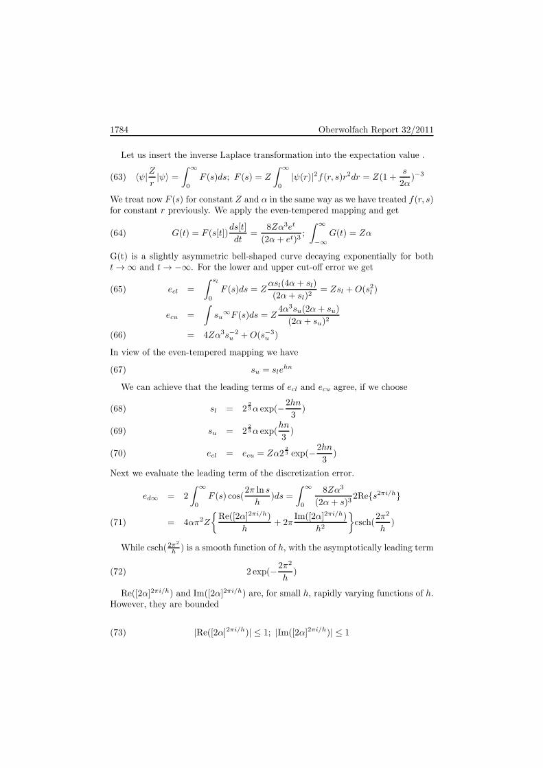
1784 Oberwolfach Report 32/2011
Let us insert the inverse Laplace transformation into the expectation value .
(63) 〈ψ|Zr|ψ〉 =
∫ ∞
0
F (s)ds; F (s) = Z
∫ ∞
0
|ψ(r)|2f(r, s)r2dr = Z(1 +s
2α)−3
We treat now F (s) for constant Z and α in the same way as we have treated f(r, s)for constant r previously. We apply the even-tempered mapping and get
(64) G(t) = F (s[t])ds[t]
dt=
8Zα3et
(2α+ et)3;
∫ ∞
−∞G(t) = Zα
G(t) is a slightly asymmetric bell-shaped curve decaying exponentially for botht→∞ and t→ −∞. For the lower and upper cut-off error we get
ecl =
∫ sl
0
F (s)ds = Zαsl(4α+ sl)
(2α+ sl)2= Zsl +O(s2l )(65)
ecu =
∫su
∞F (s)ds = Z4α3su(2α+ su)
(2α+ su)2
= 4Zα3s−2u +O(s−3
u )(66)
In view of the even-tempered mapping we have
(67) su = slehn
We can achieve that the leading terms of ecl and ecu agree, if we choose
sl = 223α exp(−2hn
3)(68)
su = 223α exp(
hn
3)(69)
ecl = ecu = Zα223 exp(−2hn
3)(70)
Next we evaluate the leading term of the discretization error.
ed∞ = 2
∫ ∞
0
F (s) cos(2π ln s
h)ds =
∫ ∞
0
8Zα3
(2α+ s)32Res2πi/h
= 4απ2Z
Re([2α]2πi/h)
h+ 2π
Im([2α]2πi/h)
h2
csch(
2π2
h)(71)
While csch(2π2
h ) is a smooth function of h, with the asymptotically leading term
(72) 2 exp(−2π2
h)
Re([2α]2πi/h) and Im([2α]2πi/h) are, for small h, rapidly varying functions of h.However, they are bounded
(73) |Re([2α]2πi/h)| ≤ 1; |Im([2α]2πi/h)| ≤ 1

Mathematical Methods in Quantum Chemistry 1785
If we consider further that the asymptotic behaviour of ed∞ is determined by theterms with 1
h2 , we get the following asymptotic estimate
(74) |ed∞| ≤ edas = 8αZπ3h−2 exp(−2π2
h)
The overall error is determined by the factor exp(−2π√
n3 ).
The expansion of 1r in a Gaussian basis follows similar patterns, but the algebra
is more complicated.
References
[1] R. N. Hill, J. Chem. Phys. 83, 1173 (1985)[2] W. Kutzelnigg, Theor. Chim. Acta 1985; W. Klopper and W. Kutzelnigg, Chem. Phys. Lett.
134, 17 (1987)[3] T. Kato, Comm. Pure Appl. Math. 10, 151 (1957)[4] F. Stenger, Numerical Methods based on Sinc and Analytical Functions, Springer, New
York, 1993[5] I. Shavitt and M. Karplus, J. Chem. Phys. 36, 550 (1962)[6] W.Kutzelnigg, Int. J. Quantum Chem. 51, 447 (1994); W. Kutzelnigg, AIP conference
proceedings 2011, in press[7] W.Kutzelnigg, J. Chem. Phys. 126, 201103 (2007)[8] D. Braess, W. Hackbusch,’Approximation of 1/x by Exponential Sums in [1,∞ ), IMA J.
num. anal. 25, 685 (2005)
Electrons in Spherical Confining Potentials
Jerzy Cioslowski
The talk concerns two recent developments in the field of Coulombic systemssubject to spherical confinements, namely:
1. Shell Model Of Assemblies Of Equicharged Particles Subject To
Radial Confining Potentials
A shell model of an assembly of N equicharged particles subject to an arbitraryradial confining potential N W (r), where W (r) is parameterized in terms of anauxiliary function Λ(t), is presented. The validity of the model requires thatΛ(t) is strictly increasing and concave for any t ∈ (0, 1), Λ′(0) is infinite, and
Λ(t) = −t−1Λ′(t)/Λ′′(t) is finite at t = 0. At the bulk limit of N →∞, the modelis found to correctly reproduce the energy per particle pair and the mean crystalradius R(N), which are given by simple functionals of Λ(t) and Λ′(t), respectively.Explicit expressions for an upper bound to the cohesive energy and the large-N asymptotics of R(N) are obtained for the first time. In addition, variationalformulation of the cohesive energy functional leads to a closed-form asymptoticexpression for the shell occupancies. All these formulae involve the constant ξ thatenters the expression −(ξ/2)n3/2 for the leading angular-correlation correction tothe minimum energy of n electrons on the surface of a sphere with a unit radius (thesolution of the Thomson problem). The approximate energies, which constituterigorous upper bounds to their exact counterparts for any value of N , include

1786 Oberwolfach Report 32/2011
the cohesive term that is not accounted for by the mean-field (fluid-like) theoryand its simple extensions but completely neglect the surface-energy correctionproportional to N .
References
[1] J.Cioslowski and E.Grzebielucha: Physical Review A 77 (2008) 032508 Strong-CorrelationLimit of Four Electrons in an Isotropic Harmonic Trap
[2] J.Cioslowski and M.Buchowiecki: Chemical Physics Letters 456 (2008) 146 Coulomb Crys-tals of Few Particles: Closed-Form Expressions for Equilibrium Energies and Geometries,and Vibrational Force Constants
[3] J.Cioslowski: Journal of Chemical Physics 128 (2008) 164713 Properties of Coulomb Crys-tals: Rigorous Results
[4] J.Cioslowski and E.Grzebielucha: Physical Review E 78 (2008) 026416 Parameter-FreeShell Model of Spherical Coulomb Crystals
[5] J.Cioslowski and E.Grzebielucha: Journal of Chemical Physics 130 (2009) 094902 Zero-Point Vibrational Energies of Spherical Coulomb Crystals
[6] J.Cioslowski: Physical Review E 79 (2009) 046405 Modified Thomson Problem[7] J.Cioslowski and E.Grzebielucha: Journal of Chemical Physics 132 (2010) 024708
Screening-Controlled Morphologies of Yukawa Crystals[8] J.Cioslowski: Journal of Chemical Physics 133 (2010) 234902 Shell Structures of Assemblies
of Equicharged Particles Subject to Radial Power-Law Confining Potentials[9] J.Cioslowski and E.Grzebielucha: Journal of Chemical Physics 134 (2011) 124305 Shell
Model of Assemblies of Equicharged Particles Subject to Radial Confining Potentials
2. The Weak-correlation Limit Of Three-dimensional Quantum Dots
With Three Electrons
Asymptotic energy expressions for the weak-correlation limits of the two lowest-energy states of three-dimensional quantum dots with three electrons are obtainedin closed forms. When combined with the known results for the strong-correlationlimit, those expressions, which are correct throughout the second order of pertur-bation theory, yield robust Pade approximants that allow accurate estimation ofenergies in question for all magnitudes of the confinement strength.
References
[1] E.Matito, J.Cioslowski, and S.F.Vyboishchikov: Physical Chemistry Chemical Physics 12(2010) 6712 Properties of Harmonium Atoms from FCI Calculations: Calibration andBenchmarks for the Ground State of the Two-Electron Species
[2] J.Cioslowski and E.Matito: Journal of Chemical Physics 134 (2011) 116101 The WeakCorrelation Limit of the Three-Electron Harmonium Atom
[3] J.Cioslowski and E.Matito: Journal of Chemical Theory and Computation 7 (2011) 915Benchmark Full Configuration Interaction Calculations on the Lowest-Energy 2P and 4PStates of the Three-Electron Harmonium Atom

Mathematical Methods in Quantum Chemistry 1787
Local defects in quantum crystals
Eric Cances
(joint work with A. Deleurence, V. Ehrlacher, M. Lewin)
The modelling and simulation of the electronic structure of crystals is a promi-nent topic in solid-state physics, materials science and nano-electronics. Besidesits importance for the applications, it is an interesting context for mathemati-cians for it gives rise to many interesting mathematical and numerical questions.The mathematical difficulties originate from the fact that crystals consist of in-finitely many charged particles (positively charged nuclei and negatively chargedelectrons) interacting with Coulomb potential. Of course, a real crystal containsa finite number of particles, but in order to understand and compute the macro-scopic properties of a crystal from first principles, it is in fact easier, or at leastnot more complicated, to consider that we are dealing with an infinite system.
The first mathematical studies of the electronic structure of crystals were con-cerned with the so-called thermodynamic limit problem for perfect crystals. Asopposed to real crystals, which contain local defects (vacancies, interstitial atoms,impurities) and extended defects (dislocations, grain boundaries), perfect crystalsare periodic arrangements of nuclei and electrons, in the sense that both the nu-clear density and the electronic density are R-periodic distributions, R denotingsome discrete periodic lattice of R3. The thermodynamic limit problem for perfectcrystals can be stated as follows. Starting from a given electronic structure modelfor finite molecular systems, find an electronic structure model for perfect crys-tals, such that when a cluster grows and “converges” (in some sense, see [5]) tosome R-periodic perfect crystal, the ground state electronic density of the clusterconverges to the R-periodic ground state electronic density of the perfect crystal.
For Thomas-Fermi like models, it is not difficult to guess what should be thecorresponding models for perfect crystals. On the other hand, solving the thermo-dynamic limit problem, that is proving the convergence property discussed above,is much more difficult. This program was carried out for the Thomas-Fermi (TF)model in [12] and for the Thomas-Fermi-vonWeizsacker (TFW) model in [5]. Notethat these two models are strictly convex in the density, and that the uniquenessof the ground state density is an essential ingredient of the proof.
The case of Hartree-Fock and Kohn-Sham like models is more involved. In thesemodels, the electronic state is described in terms of electronic density matrices.For a finite system, the ground state density matrix is a non-negative trace-classself-adjoint operator, with trace N , the number of electrons in the system. Forinfinite systems, the ground state density matrix is no longer trace-class, whichsignificantly complicates the mathematical arguments. Yet, perfect crystals beingperiodic, it is possible to make use of Bloch-Floquet theory and guess the structureof the periodic Hartree-Fock and Kohn-Sham models. These models are widelyused in solid-state physics and materials science. The thermodynamic limit prob-lem seems out of reach with state-of-the-art mathematical tools, except in thespecial case of the restricted Hartree-Fock (rHF) model, also called the Hartree

1788 Oberwolfach Report 32/2011
model in the physics literature. Thoroughly using the strict convexity of the rHFenergy functional with respect to the electronic density, Catto, Le Bris and Lionswere able to solve the thermodynamic limit problem for the rHF model [6].
Very little is known about the modelling of perfect crystals within the frame-work of the N -body Schrodinger model. To the best of our knowledge, the onlyavailable results [7, 10] state that the energy per unit volume is well defined in thethermodynamic limit. So far, the Schrodinger model for periodic crystals is stillan unknown mathematical object.
The mathematical analysis of the electronic structure of crystals with defectshas been initiated in [2] for the rHF model. This work is based on a simpleidea whose rigorous implementation however requires some effort. This idea isvery similar to that used in [8, 9] to properly define a no-photon QED model foratoms and molecules. Loosely speaking, it consists in considering the defect (theatom or the molecule in QED) as a quasiparticle embedded in a well-characterizedbackground (a perfect crystal in our case, the polarized vacuum in QED), and tobuild a variational model allowing to compute the ground state of the quasiparticle.
In [2], such a variational model is obtained by passing to the thermodynamiclimit in the difference between the ground state density matrices obtained respec-tively with and without the defect (and with periodic boundary conditions). TherHF ground state density matrix of an insulating or semiconducting crystal in thepresence of a local defect can be written as γ = γ0per+Q, where γ0per is the density
matrix of the host perfect crystal (an orthogonal projector on L2(R3) with infiniterank which commutes with the translations of the lattice) and Q a self-adjointHilbert-Schmidt operator on L2(R3). Although Q is not trace-class in general [4],it is possible to give a sense to its generalized trace Tr0(Q) := Tr(Q++)+Tr(Q−−),where
Q++ := (1− γ0per)Q(1− γ0per) and Q−− := γ0perQγ0per
(as γ0per is an orthogonal projector, Tr = Tr0 on the space of the trace-class
operators on L2(R3)), as well as to its density ρQ. The latter is defined by
∀W ∈ C∞c (R3), Tr0(QW ) =
∫
R3
ρQW.
The function ρQ is not in L1(R3) in general, but only in L2(R3) ∩ C, where C isthe Coulomb space, that is the space of charge distributions with finite Coulombenergy. An important consequence of these results is that
• in general, the electronic charge of the defect can be defined neither asTr(Q) nor as
∫R3 ρ;
• it may happen that ρQ ∈ L1(R3) but Tr0(Q) 6=∫R3 ρQ (while we would
have ρQ ∈ L1(R3) and Tr0(Q) = Tr(Q) =∫R3 ρQ if Q were a trace-class
operator). In this case, Tr0(Q) and∫R3 ρQ can be interpreted respectively
as the bare and renormalized electronic charges of the defect [4].
For a given nuclear charge of the defect, the bare (resp. the renormalized) elec-tronic charge of the defect can a priori take several values [3], depending on the
Mathematical Methods in Quantum Chemistry 1789
choice of the Fermi level (i.e. of the chemical potential of the electrons). Yet,if the Coulomb energy of the nuclear charge ν of the defect is small enough andif m is integrable, the bare and renormalized electronic charges of the defect areindependent of the choice of the Fermi level, and are respectively equal to 0 andL0
1+L0
∫R3 ν, where 0 < L0 <∞ is a constant depending only on the host crystal [4].
Consequenly the renormalized total charge is given by∫
R3
ν − L0
1 + L0
∫
R3
ν =
∫R3 ν
(1 + L0).
The charge ν is thus partially screened by a factor 1 < (1+L0) <∞. Full screeningwould correspond to L0 = +∞ and to a renormalized total charge equal to zero.
Let us emphasize that the results in [2, 4] are limited to insulators and semicon-ductors, characterized in the rHF setting by the fact that there is a positive gapbetween the Zth and (Z+1)st bands of the spectrum of the mean-field Hamiltonianof the perfect crystal, where Z is the number of electrons per unit cell. The math-ematical arguments in [2, 4] cannot be straightforwardly adapted to the “metallic”case (absence of gap). In [12], Lieb and Simon have proved full screening for theTF model, under the assumption that the host crystal is a homogeneous medium.In [1], we focus on the TFW model [11] and prove that, in this framework, defectsare always neutral (the charge ν is fully screened). As a consequence, the TFWmodel cannot be used to model insulating or semiconducting crystals, for whichthe screening effect is only partial, and in which charged defects can be observed.
References
[1] E. Cances and V. Ehrlacher, A mathematical formulation of the random phase approxima-tion for crystals, Arch. Ration. Mech. Anal., in press.
[2] E. Cances, A. Deleurence, and M. Lewin, A new approach to the modeling of local defectsin crystals: the reduced Hartree-Fock case, Commun. Math. Phys. 281 (2008), 129–177.
[3] E. Cances, A. Deleurence, and M. Lewin, Non-perturbative embedding of local defects incrystalline materials, J. Phys.: Condens. Matter 20 (2008), 294213.
[4] E. Cances and M. Lewin, The dielectric permittivity of crystals in the reduced Hartree-Fockapproximation, Arch. Ration. Mech. Anal. 197 (2010), 139–177.
[5] I. Catto, C. Le Bris and P.-L. Lions, Mathematical theory of thermodynamic limits -Thomas-Fermi type models, Oxford University Press, New York (1998).
[6] I. Catto, C. Le Bris and P.-L. Lions, On the thermodynamic limit for Hartree-Fock typemodels, Ann. Inst. H. Poincare Anal. Non Lineaire 18 (2001),687–760.
[7] C. Fefferman, C., The thermodynamic limit for a crystal, Commun. Math. Phys. 98 (1985),289–311.
[8] C. Hainzl, M. Lewin, M. and Sere, A minimization method for relativistic electrons in amean-field approximation of quantum electrodynamics, Phys. Rev. A 76 (2007), 052104.
[9] C. Hainzl, M. Lewin, and J.P.Solovej, The mean-field approximation in electrodynamics:the no-photon case, Commun. Pure Appl. Math. 60 (2007), 546–596.
[10] C. Hainzl, M. Lewin, and J.P. Solovej, The thermodynamic limit of quantum Coulombsystems, Advances in Math. 221 (2009), 454–546.
[11] E.H. Lieb, Thomas-Fermi and related theories of atoms and molecules, Rev. Mod. Phys.53 (1981), 603–641.
[12] E.H. Lieb and B. Simon, The Thomas-Fermi theory of atoms, molecules and solids, Ad-vances in Math. 23 (1977), 22–116.

1790 Oberwolfach Report 32/2011
How Much Energy Does it Cost to Make a Hole in the Fermi Sea?
Mathieu Lewin
(joint work with Rupert L. Frank, Elliott H. Lieb and Robert Seiringer)
Before addressing the question in the title, let us go back in time and discuss asimpler problem, which has been solved by Lieb and Thirring [8, 9] in 1975. Givena density ρ(r) (a positive integrable function on R3), what is the kinetic energycost to create a pile of N =
∫R3 ρ(r) dr electrons having the given density ρ(r)?
Because an electron can be given large momentum without changing its density,this energy can be arbitrarily large and a better question is to ask for the minimalkinetic energy cost.
Let us formalize this mathematically. The kinetic energy of any (mixed) quan-tum state can be expressed as tr(−∆γ), where γ is the corresponding one-particledensity matrix [7], ∆ = ∇2 being the Laplacian (in units such that m = 1/2 and~ = 1). The self-adjoint operator γ acts on L2(R3,Cq) where q is the number ofinternal degrees of freedom (q = 2 for electrons) and it must satisfy the followingconstraint 0 ≤ γ ≤ 1 in the sense of self-adjoint operators. The kernel γ(r, r′)σ,σ′
of γ is a q×q matrix for every (r, r′) ∈ R6 and the corresponding density is definedas ργ(r) =
∑qσ=1 γ(r, r)σ,σ.
Coleman has shown in [1] that there is no further necessary condition on γ, thatis, any operator 0 ≤ γ ≤ 1 with trγ =
∫R3 ργ = N arises from at least one (mixed)
N -body quantum state. This allows us to define the minimal energy cost as
(1) T (ρ) = inf0≤γ≤1ργ=ρ
tr(−∆γ).
In a semi-classical approximation, we think of putting the electrons in smallboxes in phase space, of volume (2π)3. The semi-classical approximation to T (ρ)is then [12, 3]
Tsc(ρ) = (2π)−3q
∫
R3
dr
∫
p≤(
6π2ρ(r)q
)1/3 p2 dp = Ksc(3)
∫
R3
ρ(r)53 dr,
where Ksc(3) = (3/5)(6π2/q)2/3. Lieb and Thirring have shown in [8, 9] that,up to a universal constant, semi-classics provides a universal lower bound to thetrue minimal quantum energy cost, even far from the semi-classical regime. Thestatement in any dimension is
(2) T (ρ) ≥ K(d)
∫
Rd
ρ(r)1+d2 dr
where K(d) is a universal constant depending only on the space dimension d, andsuch that
K(d) ≤ Ksc(d) :=d
d+ 2
(d(2π)d
q |Sd−1|
)2d
.

Mathematical Methods in Quantum Chemistry 1791
It is widely believed that K(d) = Ksc(d) for d ≥ 3. The best estimate known so
far in dimension 3 is K(3) ≥ 0.6724 Ksc(3), see [2]. Since its invention, the Lieb-Thirring inequality has played an important role for the study of large quantumsystems and of their stability [6, 7].
The dual version of the Lieb-Thirring inequality (2) is sometimes useful. LetV (r) be a real-valued potential (the variable dual to ρ(r)). The sum of the negativeeigenvalues of −∆+ V (r) can be expressed by a variational principle, leading tothe estimate∑
λi≤0
λi(−∆+ V ) = inf0≤γ≤1
tr((−∆+ V )γ
)
≥ infρ≥0
∫
Rd
(K(d)ρ(r)1+2/d + V (r)ρ(r)
)dr
= −L(d)∫
Rd
V (r)1+d/2− dr,(3)
where x− = −min(0, x) is the negative part of a number x and
L(d) =2
d+ 2
(d
(d+ 2) K(d)
)d/2
.
It can actually be shown that the inequality (3) is equivalent to (2).
A question that is not only natural but of significance for condensed matterphysics is the analogue of (2) when we start, not with the vacuum, but with abackground of fermions with some prescribed density ρ0 > 0. In [4], we haveestimated the minimal energy cost to go from an infinitely extended free Fermigas of constant density ρ0 > 0 to a density ρ(r) = ρ0 + δρ(r). Note that δρ(r) hasno sign a priori. It can be negative (hence the word ‘hole’ in our title) as soon asδρ(r) ≥ −ρ0. The main difficulty is that we are perturbing an infinite quantumsystem, spread over the whole space. Nevertheless, we have been able to provethat semi-classics again gives a lower bound to the energy cost.
To formulate our result properly, let us recall that the Fermi level µ is linkedto the density ρ0 by the formula
ρ0 =q
(2π)d
∫
k2≤µ
dk =q |Sd−1|d (2π)d
µd2
in any dimension d ≥ 1. The one-particle density matrix of the free Fermi sea isthe spectral projector Π− := χ(−∞,µ)(−∆) corresponding to filling all the energies≤ µ. Our inequality can now be stated as follows, in space dimensions d ≥ 2:
(4) tr (−∆− µ) (γ −Π−)
≥ K(d)
∫
Rd
(ργ(r)
1+2d − (ρ0)
1+2d − 2 + d
d(ρ0)
2d(ργ(r) − ρ0
))dr
for any one-particle density matrix 0 ≤ γ ≤ 1. The term on the left side isnon-negative, which follows from the fact that Π− minimizes the free energy withchemical potential µ. The integrand on the right side is also non-negative, which

1792 Oberwolfach Report 32/2011
follows this time from the convexity of ρ 7→ ρ1+2/d. It behaves like (ρ(r) − ρ0)2for ρ(r) ≃ ρ0 and like ρ(r)1+2/d for large ρ(r), as in the usual Lieb-Thirringinequality (2). Taking ρ0 → 0 we actually recover (2) in the limit. The optimalconstant K(d) is independent of ρ0 > 0 (by scaling) but it does not necessarily
coincide with the optimal constant K(d) of (2) for ρ0 = 0. The inequality (4) isnot valid in dimension d = 1, as we will explain later.
As for the usual Lieb-Thirring case, there is a dual inequality. Let us considera real-valued potential V (r) ∈ L2(Rd) ∩ L1+d/2(Rd), for d ≥ 2. Then we have
(5) tr(−∆− µ+ V )(Π−V −Π−)
≥ −L(d)∫
Rd
((V (r) − µ)1+
d2
− − µ1+d2 +
2 + d
2µ
d2 V (r)
)dr,
where Π−V := χ(−∞,µ)(−∆+V ) is the one-particle density matrix of the perturbed
Fermi sea in presence of the potential V . The integrand on the right side behaves
like V (r)2 for small V (r) and V (r)1+d/2− for large V (r). The left side is formally
equal to
tr(−∆−µ+V )(Π−V −Π−)“ = ”− tr(−∆+V −µ)−+tr(−∆−µ)−−ρ0
∫
R3
V (r) dr
but the first two terms on the right are infinite and the third is only finite underthe additional assumption that V ∈ L1(Rd). Note that the term ρ0
∫R3 V (r) dr is
obtained by first order perturbation theory.Second order perturbation theory predicts that
(6) limǫ→0
tr(−∆− µ+ ǫV )(Π−ǫV −Π−)
ǫ2= −µ
d2−1
∫
Rd
Ψd
(kõ
)|V (k)|2 dk
where Ψd is the linear response function of the Fermi sea, which can be computedexplicitly. In dimension d = 1,
Ψ1(|k|) =1
4π|k| log(
2 + |k|∣∣2− |k|∣∣
)
is divergent at k = ±2, which is related to the so-called Peierls instability [10]. Onthe contrary, the semi-classical function satisfies
limǫ→0
∫
Rd
dr(ǫV (r)− µ)1+
d2
− − µ1+d2 + 2+d
2 µd2 ǫV (r)
ǫ2= −d(d+ 2)
8µ
d2−1
∫
Rd
V (r)2dr
in any dimension d ≥ 1. This proves that there cannot be a Lieb-Thirring inequal-ity of the form of (5) in dimension d = 1. In higher dimensions d ≥ 2, Ψd is abounded function and there is no problem.
In the original works [8, 9], the potential Lieb-Thirring estimate (3) was derivedfirst by spectral methods and the density estimate (2) was then obtained by usingthe equivalence. Until recently, there was no known direct proof of the densityestimate (2). The situation changed last year when Rumin [11] found a simple

Mathematical Methods in Quantum Chemistry 1793
method to directly prove (2). Our method to tackle the positive density estimateshow (4) is partly based on Rumin’s ideas.
Our estimates (4) and (5) can be generalized in several directions. They arevalid at positive temperature, and also when the ideal Fermi gas is replaced by aperiodic background, under generic assumptions on the Fermi surface [5].The research leading to these results has received funding from the European Re-search Council under the European Community’s Seventh Framework Programme(FP7/2007-2013 Grant Agreement MNIQS No. 258023).
References
[1] A. Coleman, Structure of fermion density matrices, Rev. Modern Phys., 35 (1963), pp. 668–689.
[2] J. Dolbeault, A. Laptev, and M. Loss, Lieb-Thirring inequalities with improved con-stants, J. Eur. Math. Soc. (JEMS), 10 (2008), pp. 1121–1126.
[3] E. Fermi, Un metodo statistico per la determinazione di alcune priorieta dell’atome, Rend.Accad. Naz. Lincei, 6 (1927), pp. 602–607.
[4] R. L. Frank, M. Lewin, E. H. Lieb, and R. Seiringer, Energy Cost to Make a Hole inthe Fermi Sea, Phys. Rev. Lett., 106 (2011), p. 150402.
[5] , An analogue of the Lieb-Thirring inequality at positive density. In preparation, 2011.[6] E. H. Lieb, The stability of matter, Rev. Mod. Phys., 48 (1976), pp. 553–569.[7] E. H. Lieb and R. Seiringer, The Stability of Matter in Quantum Mechanics, Cambridge
Univ. Press, 2010.[8] E. H. Lieb and W. E. Thirring, Bound on kinetic energy of fermions which proves stability
of matter, Phys. Rev. Lett., 35 (1975), pp. 687–689.[9] , Inequalities for the moments of the eigenvalues of the Schrodinger hamiltonian and
their relation to Sobolev inequalities, Studies in Mathematical Physics, Princeton UniversityPress, 1976, pp. 269–303.
[10] R. E. Peierls, Quantum Theory of Solids, Clarendon Press, 1955.[11] M. Rumin, Balanced distribution-energy inequalities and related entropy bounds.
arXiv:1008.1676, 2010.[12] L. H. Thomas, The calculation of atomic fields, Proc. Camb. Philos. Soc., 23 (1927),
pp. 542–548.
Towards the optimal basis set in Kohn-Sham density functional theory
Lin Lin
(joint work with Weinan E, Jianfeng Lu and Lexing Ying)
Kohn-Sham density functional theory (KSDFT) is by far the most widely usedelectronic structure theory for condensed matter systems. However, the compu-tational cost of the standard method for solving KSDFT increases cubically withrespect to the number of electrons in the system (N). The cubic scaling hindersthe application of KSDFT to systems of large size.
Our aim is to design accurate and efficient algorithms to solve KSDFT for bothinsulating and metallic systems [1, 2, 3, 4, 5, 6, 7]. The electron density ρ dependsonly on the diagonal of the Fermi-Dirac operator (β: inverse temperature; µ:
1794 Oberwolfach Report 32/2011
chemical potential)
(1) ρ = diag f(H) ≡ diag2
1 + eβ(H−µ).
Our method directly targets at the calculation of the diagonal elements of theFermi-Dirac operator, and thus reduces the computational cost for solving KSDFT.Specifically, the computational cost of our method is O(N) for one dimensionalsystems, O(N1.5) for two-dimensional systems, and O(N2) for three-dimensionalsystems.
In this talk I focus on the reduction of the discretization cost for solving KS-DFT. The discretization cost is characterized by the number of basis functions peratom to discretize the Kohn-Sham Hamiltonian operator, and is a crucial factorin the total computational cost. Take the planewave discretization for instance,the number of basis functions is generally 500 ∼ 5000 even in the pseudopotentialframework. The discretization cost can be significantly reduced to 20 ∼ 80 ba-sis functions per atom by means of e.g. atomic orbital type basis functions, butthese basis functions are based on explicit knowledge of the underlying system,and are often difficult to be systematically improved in practice. To overcome theproblem of both the planewave basis functions and the atomic orbital type basisfunctions, we propose a novel discretization scheme called the adaptive local basisfunctions [4]. The adaptive local basis functions do not require explicit knowl-edge of the system, and are systematically obtained by solving a series of KSDFTproblems of small size. The adaptive local basis functions achieve high accuracy(below 10−3 Hartree/atom) in the total energy calculation with the number ofbasis functions per atom close to the minimum possible number, namely the num-ber of basis functions used by the tight binding method. The adaptive local basisfunctions are localized in the real space, and are discontinuous in the global do-main. The continuous Kohn-Sham orbitals and the electron density are evaluatedfrom these discontinuous basis functions using the discontinuous Galerkin (DG)framework. We demonstrate that primitive implementation of the adaptive localbasis functions is already able to calculate the total energy for systems consistingof thousands of atoms.
The adaptive local basis functions are accurate, efficient, simple and systemat-ically improvable in the total energy calculation. One potential drawback of theadaptive local basis functions is that the accuracy of the force calculation may notbe systematically controlled. It is well known that if the basis functions changewith respect to the atomic positions, the Hellmann-Feynman force is not accurateenough, and the Pulay force should be added [8]. The calculation of the Pulayforce can be expensive since the derivatives of the basis functions with respectto all the atomic positions are to be computed. To overcome this drawback, wedevelop the optimized local basis functions [5] that inherit all the advantages ofthe adaptive local basis functions, and can systematically improve the accuracy ofthe force calculation. The optimized local basis functions are obtained by solvinga variational problem in a prescribed primitive basis set that is independent ofthe atomic positions. When the optimality condition is satisfied, the contribution
Mathematical Methods in Quantum Chemistry 1795
of the Pulay force vanishes and the total force is equal to the Hellmann-Feynmanforce. This makes the optimized local basis functions an ideal tool for ab initiomolecular dynamics as well as geometry optimization. We develop a precondi-tioned GMRES algorithm to obtain the optimized local basis functions in prac-tice. Numerical results using a one dimensional model problem indicate that theoptimized local basis functions can accurately compute the energy and the forcealong the trajectory of the molecular dynamics without systematic drift, using avery small number of basis functions per atom.
References
[1] L. Lin, J. Lu, R. Car, and W. E. Multipole representation of the Fermi operator with ap-plication to the electronic structure analysis of metallic systems. Phys. Rev. B, 79:115133,2009.
[2] L. Lin, J. Lu, L. Ying, R. Car, and W. E. Fast algorithm for extracting the diagonal ofthe inverse matrix with application to the electronic structure analysis of metallic systems.Comm. Math. Sci., 7:755, 2009.
[3] L. Lin, J. Lu, L. Ying, and W. E. Pole-based approximation of the Fermi-Dirac function.Chinese Ann. Math., 30B:729, 2009.
[4] L. Lin, J. Lu, L. Ying, and W. E. Adaptive local basis set for Kohn-Sham density functionaltheory in a discontinuous Galerkin framework I: Total energy calculation. submitted, 2011.
[5] L. Lin, J. Lu, L. Ying, and W. E. Optimized local basis function for Kohn-Sham densityfunctional theory. in preparation, 2011.
[6] L. Lin, C. Yang, J. Lu, L. Ying, and W. E. A fast parallel algorithm for selected inversion ofstructured sparse matrices with application to 2D electronic structure calculations. SIAM J.Sci. Comput., 33:1329, 2011.
[7] L. Lin, C. Yang, J. Meza, J. Lu, L. Ying, and W. E. SelInv – An algorithm for selectedinversion of a sparse symmetric matrix. ACM. Trans. Math. Software, 37:40, 2010.
[8] P. Pulay. Ab initio calculation of force constants and equilibrium geometries in polyatomicmolecules I. Theory. Mol. Phys., 17:197, 1969.
A Modified Born–Oppenheimer Approximation for Hydrogen Bonding
George A. Hagedorn
(joint work with Alain Joye)
The standard time–independent Born–Oppenheimer approximation often yieldssubstantially inaccurate vibrational energy levels for molecules that contain hy-drogen bonds. In particular, the vibrational energy levels associated with oscilla-tions of the hydrogen nucleus involved in the hydrogen bonding are often far fromaccurate. In this talk, we summarize the results of a joint project with Alain Joyeto produce a better approximation that is still amenable to practical computation.
The detailed results of the project are presented in two papers, [5, 7]. Twoother summaries (and a generalization) are presented in conference proceedingsarticles, [6, 8].
The reason the results were published in two separate papers is that we con-sidered two different situtations. In the first paper, [5], we studied the symmetrichydrogen bonds. In this case, we considered a molecule that consisted of two iden-tical components that were bound together by a hydrogen bond. The molecule

1796 Oberwolfach Report 32/2011
thus had a reflection symmetry. As an example, we presented detailed results forthe FHF− ion. In the second paper, [7], we studied the situation where there wasno such symmetry. The concrete example we presented was the FHCl− ion.
As we were completing this work, we learned of a related paper, [10], that empir-ically related vibrational energies of protons involved in hydrogen bonds with howsymmetrical the hydrogen bond was. That paper considered some non-symmetricmolecules that were very close to being symmetrical. In practice, our resultsare not likely to yield much useful information in these “almost symmetrical”situations since they are near the borderline between our two different modifiedapproximations.
Standard Born–Oppenheimer approximations rely on the smallness of the pa-rameter ǫ, where the nuclear masses are taken proportional to ǫ−4 and the electronmasses are held fixed. The original work in this subject is [1], and there is now asubstantial mathematical literature on this subject. See, e.g., [2, 3, 4, 9]. Molecu-lar energy levels have asymptotic expansions to all orders in even powers of ǫ. Theǫ0 term arises from the energy of the electrons with the nuclei at optimal config-urations. The ǫ2 term consists of the harmonic approximations to the vibrationsof the nuclei about the optimal configurations. The ǫ4 term contains an electronenergy correction, the lowest order anharmonic corrections to the vibrational en-ergies, an uninteresting term related to removal of the center of mass motion, andthe leading order rotational energy of the molecule.
For symmetric hydrogen bonds, we make two modifications. First, we take themass of the hydrogen nucleus to be proportional to ǫ−3. This is motivated by theobservation that if the nucleus of (the most common isotope of) carbon is ǫ−4,then the mass of a hydrogen nucleus is 1.015 ǫ−3. Second, the electron energylevel is the effective potential felt by the nuclei, and we modify one coefficientin its Taylor series approximation around the optimal nuclear configuration. If Zdenotes the coordinate for the hydrogen nucleus between the other two componentsof the molecule, we replace the quadratic term in the Taylor approximation, aZ2,by (a/ǫ) ǫ Z2. We numerically divide in the factor (a/ǫ) with the true value ofǫ = 0.0821, but algebraically multiply by the small parameter ǫ. This is motivatedby looking at examples and observing that the typical value of a is small in realmolecules, and that (a/0.0821) is typically roughly of order 1.
Thus, in our model, the small parameter ǫ plays two roles. It is involved in thescaling of the masses, and it also appears in the expression we use for the electronicpotentially energy surface.
In the symmetric situation, we prove that with this modified model, the molec-ular energy has a full asymptotic expansion in powers of ǫ1/2. Our main interestis in the vibrational energies, which appear to leading order at order ǫ2, as inthe standard approximation. However, they are not described by a harmonic os-cillator. To leading order, they are described by the energy levels of a quantumHamiltonian that contains certain cubic and quartic terms as well as quadraticterms.

Mathematical Methods in Quantum Chemistry 1797
For the FHF− ion, the standard harmonic approximation predicts the energyof the “asymmetric stretch,” in which the hydrogen nucleus oscillates between itsheavier neighbors, to be 1118 cm−1, whereas an experimental value is 1331 cm−1.Our model produces a much more accurate 1399 cm−1.
For non-symmetric hydrogen bonds, we again modeled the hydrogen mass by1.015 ǫ−3, but this time we made a different modification to the electronic poten-tial energy surface. In the Taylor expansion, we made no changes to the termsthat involved the hydrogen nucleus and its closest neighboring nucleus. For allterms that involve the heavy nucleus of the hydrogen bond that is farther fromthe hydrogen nucleus, we numerically divide the coefficient by ǫ = 0.0821 andmultiply algebraically by the small parameter ǫ. This is motivated from examin-ing the electronic potential energy surface for the FHCl− ion. From numericalcalculations, this ion behaves like FH with an internuclear distance of roughly1 Angstrom, and a Cl− ion roughly 2 Angstroms for the H nucleus. Since theH–Cl− distance is large, all interactions involving the Cl− are small.
In the non-symmetric situation, our model yields an asymptotic expansion inpowers of ǫ1/4, but the vibrations associated with the hydrogen bond appear atdifferent orders. The oscillations of the bond between the hydrogen nucleus andits nearest neighbor are of order ǫ3/2; the bending vibrations occur at order ǫ2; andthe vibrations of the bond between the hydrogen nucleus and its farther neighborare of order ǫ5/2. In the standard Born-Oppenheimer approximation they all occurat order ǫ2, and one must do a matrix diagonalization to find the normal modesof oscillation. Here they are automatically separated at the different orders.
For the specific example of FHCl−, one easily sees that the vibrational en-ergies are of the various different orders, although our model yields vibarionalenergies that are similar to those obtained by the standard Born–Oppenheimerharmonic approximation. We predict FH–Cl− stretch, bending, and F–H stretchenergies of 246 cm−1, 875 cm−1, and 2960 cm−1, respectively. The correspond-ing experimental data are 275 cm−1, 843 cm−1, and 2710 cm−1. We note that246/875 ≈ 0.281 and 875/2960 ≈ 0.296 are both close to the physical ǫ1/2 ≈ 0.287.Thus, these energies are consistent with their appearing in our approach at ordersǫ5/2, ǫ2, and ǫ3/2, respectively.
References
[1] M. Born and J. R. Oppenheimer Zur Quantentheorie der Molekeln, Ann. Phys. (Leipzig)84 (1927) 457–484.
[2] J.-M. Combes, P. Duclos, and R. Seiler The Born–Oppenheimer Approximation, Rigorous
Atomic and Molecular Physics (ed. by G. Velo, A. Wightman, New York, Plenum, 1981,185–212.
[3] G. A. Hagedorn High Order Corrections to the Time–Independent Born–Oppenheimer Ap-proximation I: Smooth Potentials Ann. Inst. H. Poincare Sect. A. 47 (1987) 1–16.
[4] G. A. Hagedorn High Order Corrections to the Time–Independent Born–Oppenheimer Ap-proximation II: Diatomic Coulomb Systems Commun. Math. Phys. 116 (1988) 23–44.
[5] G. A. Hagedorn and A. Joye A Mathematical Theory for Vibrational Levels Associated withHydrogen Bonds I: The Symmetric Case, Commun. Math. Phys. 274 (2007), 691–715.

1798 Oberwolfach Report 32/2011
[6] G. A. Hagedorn and A. Joye Vibrational Levels Associated with Hydrogen Bonds andSemiclassical Hamiltonian Normal Forms. Adventures in Mathematical Physics: Interna-tional Conference in Honor of Jean–Michel Combes on Transport and Spectral Problemsin Quantum Mechanics, September 4–6, 2006, ed. by Francois Germinet and Peter Hislop.Amer. Math. Soc. Contemporary Mathematics 447 (2007) 139–151.
[7] G. A. Hagedorn and A. Joye A Mathematical Theory for Vibrational Levels Associated withHydrogen Bonds II: The Non–Symmetric Case, Rev. Math. Phys. 21 (2009) 279–313.
[8] G. A. Hagedorn and A. Joye A Mathematical Theory for Vibrational Levels Associated withHydrogen Bonds, Few Body Systems 45 (2009) 183–186.
[9] M. Klein, A. Martinez, R. Seiler, and X. P. Wang On the Born–Oppenheimer Expansionfor Polyatomic Molecules Commun. Math. Phys. 143 (1992) 607–639.
[10] J. R. Roscioli, L. R. McCunn, and M. A. Johnson Quantum Structure of the IntermolecularProton Bond, Science 316 (2007) 249–254.
Numerical Tensor Calculus
Wolfgang Hackbusch
1. Tensor Spaces
Given vector spaces Vj (1 ≤ j ≤ d), there is a unique (algebraic) tensor space
V =⊗d
j=1 Vj . For instance, for Vj = Rnj the elementary tensors v =⊗d
j=1 v(j)
with v(j) ∈ Rnj are defined by v[i1 . . . id] =∏d
j=1 v(j)[ij]. The tensor space is
defined by all (finite) linear combinations of elementary tensors. The dimension
of V is N :=∏d
j=1 nj .Here we consider cases, where it is impossible to store all N entries. Examples
may be nj = 1000 and d = 1000 yielding N = 10001000 as well as the naturaldimension d = 3 with nj = 106. The latter example describes a grid function on afine 3D-grid.
If the generating vector spaces Vj = Rnj×nj are matrix spaces, the tensorproduct is also called Kronecker product and produces matrices of size N ×N.
For infinite dimensional functions spaces Vj , say for uni-variate functions in xj ,
the tensor product yields d-variate functions v(x1 . . . xd) =∏d
j=1 v(j)(xj). Fixing
a suitable norm on V, the completion of the algebraic tensor space produces thetopological tensor space.
2. Representation of Tensors
Since for huge N the tensors cannot be described by all their entries, one needsa data-sparse representation. Examples are the r-term format (canonical format)
(1) v =∑r
ν=1v(j)ν for some v(j)ν ∈ Vj
and the tensor subspace format (Tucker format)
(2) v =∑r1
i1=1· · ·∑rd
id=1a[i1 . . . id]b
(1)i1⊗ . . .⊗ b(d)id
for some b(j)i1∈ Vj .

Mathematical Methods in Quantum Chemistry 1799
Fixing the representation rank r ∈ N in (1) and the vector-valued rank r =(r1 . . . rd) in (2), we obtain the sets Rr and Tr. If nj ≤ n, any v ∈ Rr require astorage of drn. For moderate r, this is feasable also for d = n = 1000. The hope isthat tensors of large or even infinite rank can be approximated in Rr for moderater. This is confirmed by the following example.
The function 1/√t can be approximated in any interval [η,∞) by exponential
sums Er(t) :=∑r
ν=1 ων exp(−ανt) (see [1]) such that the accuracy improves ex-
ponentially with r. For instance,∥∥1/√· − Er
∥∥∞,[1,∞)
=: εr ≤ 83.5 exp(−π√r/2).
Substituting the Euclidean norm t = ‖x‖2 of x ∈ Rd, we obtain an approxima-
tion of 1/ ‖x‖ by Er(‖x‖2) =∑r
ν=1 ων
∏dj=1 exp(−αν |xj |2) which belongs to Rr.
This fact can be expoited for the convolution with the Colomb potential:∥∥∥∥∫
R3
f(y)dy
‖· − y‖ −∫
R3
Er(‖· − y‖2)f(y)dy∥∥∥∥∞,R3
≤ 3.53
√‖f‖2L1 ‖f‖L∞ε
2/3r .
However, both formats mentioned above have certain disadvantages. A betterapproach is the hierarchical tensor format Hr (cf. [6], [5]). The hierarchy is givenby a certain dimension partition tree. If this tree is chosen as linear tree (maximaldepth), one obtains the so-called tensor-train format (cf. [9]). Even earlier, thelatter format has been used in quantum physics (cf., e.g., [10]) and is named‘matrix product states’ (MPS).
An important question concerns the closedness of the sets Rr, Tr, and Hr, sincefor optimisation problems we build sequences vν ∈ F (F ∈ Rr, Tr,Hr) and wantto know whether limvν ∈ F . In fact, Tr and Hr are closed (even weakly closed),but Rr is not (cf. [5]). As mentioned before, the hierarchical tensor format Hr
is structured by a tree. In quantum physics one likes to replace trees by generalgraphs. In this case, however, the set is not closed.
3. Tensor Operations and Truncation
There are various operations between tensors, one may like to compute. Westart with a simple example. Let Vj = Rnj . The Hadamard product ⊙ : Vj ×Vj →Vj is the entrywise multiplication: (v ⊙ w)i = viwi, which easily generalises totensors. The property
d⊗
j=1
v(j)
⊙
d⊗
j=1
w(j)
=
d⊗
j=1
(v(j) ⊙ w(j)
)
allows to reduce this operation to the vector spaces Vj . However, if v,w ∈ Rr
involve r terms, the product consists of r2 terms:(
r∑
ν=1
v(j)ν
)⊙(
r∑
µ=1
w(j)µ
)=
r∑
ν=1
r∑
µ=1
d⊗
j=1
(v(j)ν ⊙ w(j)
µ
).
This is a typical feature which requires a truncation step, by which one tries toapproximate the result by an expression involving fewer terms. Further operations

1800 Oberwolfach Report 32/2011
are the addition, convolution, matrix-vector and matrix-matrix multiplication andthe scalar product.
The truncation within Rr (possibly with regularisation) is not so easy (cf. [2]),whereas for the hierarchical format Hr the truncation can be based on severalsingular value decompositions (cf. [6]).
4. Tensorisation
The translation of a vector into a tensor is called ‘tensorisation’ (cf. [5]). Thesimplest case is a vector v ∈ Rn with n = 2d. Then Rn is isomorphic to the tensor
space V :=⊗d
j=1 R2. The concrete isomorphism is
Φn : V → Rn
v 7→ v with vk = v[i1 · · · id] for k =∑d
j=1 ij2j−1, 0 ≤ ij ≤ 1.
The tensor v may be represented by the tensor train representation [8] (see also[7]). The exact tensor representation is usually not interesting, since it requires thesame storage n. Instead, one looks for an approximate tensor using the truncationprocedure mentioned above.
If v ∈ Rn represents a smooth function on a grid with n point, one observes thatthe corresponding (approximate) tensor requires much less data. Typically, piece-wise smooth functions allow to reduce n to O(log(n)). The analytic background isgiven in [3]. In fact, the tensorisation corresponds to a multi-scale approach.
Operations can be applied directly to the tensorised vectors (instead to thevectors). For instance, convolution of two n-vectors which correspond to tensorsof size O(log(n)), can be performed with O(log(n)) arithmetical operations (cf.[4]).
References
[1] D. Braess, W. Hackbusch, On the efficient computation of high-dimensional integrals andthe approximation by exponential sums, in: R. DeVore, A. Kunoth (eds.) Multiscale, non-linear and adaptive approximation, pp. 39–74. Springer-Verlag, Berlin (2009)
[2] M. Espig, Effiziente Bestapproximation mittels Summen von Elementartensoren in hohenDimensionen, dissertation, Universitat Leipzig, 2008
[3] L. Grasedyck, Polynomial approximation in hierarchical Tucker format by vector-tensorization, submitted.
[4] W. Hackbusch, Tensorisation of vectors and their efficient convolution, Numer. Math., toappear
[5] W. Hackbusch, Tensor spaces and numerical tensor calculus, Monograph in preparation.[6] W. Hackbusch, S. Kuhn, A new scheme for the tensor representation, J. Fourier Anal. Appl.
15 (2009) 706–722.
[7] B.N. Khoromskij, O(d logN)-quantics approximation of N-d tensors in high-dimensionalnumerical modeling, Constr. Approx., to appear 2011
[8] I.V. Oseledets, Approximation of matrices using tensor decomposition, SIAM J. MatrixAnal. Appl. 31 (2010), 2130–2145
[9] I.V. Oseledets, E.E. Tyrtyshnikov, TT-cross approximation for multidimensional arrays,Linear Algebra Appl. 432 (2010), 70–88
[10] F. Verstraete, J.I. Cirac, Matrix product states represent ground states faithfully, Phys. Rev.B 73 (2006), 094,423

Mathematical Methods in Quantum Chemistry 1801
On the mixed regularity of electronic wavefunctions
Harry Yserentant
Atoms and molecules are physically described by the Schrodinger equation fora system of charged particles that interact by Coulomb attraction and repulsionforces. As the nuclei are much heavier than the electrons, the electrons almostinstantaneously follow their motion. Therefore it is usual in quantum chemistryto separate the motion of the nuclei from from that of the electrons, that is, tolook for the eigenvalues and eigenfunctions of the electronic Schrodinger operator
H = − 1
2
N∑
i=1
∆i −N∑
i=1
K∑
ν=1
Zν
|xi − aν |+
1
2
N∑
i,j=1i6=j
1
|xi − xj |
written down here in dimensionless form or atomic units. It acts on functions witharguments x1, . . . , xN ∈ R3, the coordinates of given N electrons. The positionsa1, . . . , aK ∈ R3 of the nuclei are kept fixed. The positive values Zν are the chargesof the nuclei in multiples of the electron charge. This talk was concerned with themixed regularity of these eigenfunctions and its implications for the complexity ofthe quantum-mechanical N -electron problem.
To state our regularity results, we need to introduce a scale of norms that isdefined in terms of Fourier transforms. These norms are given by the expression
|||u||| 2ϑ,m =
∫ 1 +
N∑
i=1
|ωi|2m N∏
i=1
(1 + |ωi|2
)ϑ
|u(ω)|2 dω.
They are defined on the Hilbert spaces Hϑ,mmix that consist of the square integrable
functions from (R3)N to R or C with Fourier transforms
u : (R3)N → C : (ω1, . . . , ωN )→ u(ω1, . . . , ωN )
for which these expressions remain finite; |ωi| is the euclidian norm of ωi. Theindex m determines the isotropic smoothness, and the index ϑ the degree of mixedregularity. For nonnegative integer values m and ϑ, the norms measure the L2-norm of weak partial derivatives. The spaces L2 and H1 belong to the class ofthese spaces. Our main result [KY] is that the eigenfunctions u of the electronicSchrodinger operator for eigenvalues below the essential spectrum are contained in
H1,0mix ∩
⋂
ϑ<3/4
Hϑ,1mix.
In the general case, the bound 3/4 can neither be completely reached nor improvedfurther. An exception are systems of electrons of the same spin, for which thewavefunctions are completely antisymmetric under the exchange of the positions ofthe electrons and vanish at the singular points of the electron-electron interactionpotential. The proof is based on a multiplicative splitting [Y2] of the wavefunctionsinto an explicitly known factor depending on the interelectronic distances and amore regular part in H1,1
mix and utilizes techniques from interpolation theory.

1802 Oberwolfach Report 32/2011
The eigenfunctions u for eigenvalues below the essential spectrum decay expo-nentially in the L2-sense. There exists a constant γ > 0 such that the function
x → exp
(γ
N∑
i=1
|xi|)u(x),
is square integrable. This constant depends on the distance of the eigenvalueunder consideration to the bottom of the essential spectrum. More details andreferences to the literature can be found in [Y1]. It has been shown in [Y2] thatthese exponentially weighted eigenfunctions admit the same kind of representa-tion as the eigenfunctions themselves. Thus they share with them the describedregularity properties [KY]. This can be used to study the expansion of the solu-tions into correspondingly antisymmetrized tensor products of three-dimensionaleigenfunctions [Y1] or orthogonal wavelets [Z], for example. It turns out that theconvergence rates of such expansions measured in terms of the number of basisfunctions involved surprisingly do not deteriorate with the number of electronsand remain comparable to those for a system of two electrons or even only oneelectron [Y1]. Therewith the curse of dimensionality is in some sense broken.
References
[KY] Kreusler, H.-C., Yserentant, H.: The mixed regularity of electronic wave functions infractional order and weighted Sobolev spaces. Preprint 94, DFG-Schwerpunktprogramm1324 (2011), http://www.dfg-spp1324.de/publications.php
[Y1] Yserentant, H.: Regularity and Approximability of Electronic Wave Functions. LectureNotes in Mathematics, vol. 2000, Springer-Verlag (2010)
[Y2] Yserentant, H.: The mixed regularity of electronic wave functions multiplied by explicitcorrelation factors. ESAIM: M2AN 45, 803–824 (2011)
[Z] Zeiser, A.: Wavelet approximation in weighted Sobolev spaces of mixed order with appli-cations to the electronic Schrodinger equation. Preprint 55, DFG-Schwerpunktprogramm1324 (2010), http://www.dfg-spp1324.de/publications.php
The regularity of tensor product approximations in L2 in dependence
of the target function
Andre Uschmajew
The approximation of a square integrable function of many variables by a sum ofproducts of functions of much fewer variables has been a prominent approach inmany fields of theory and application for a long time, the simplest example beingan expansion into a classical Fourier series. The need of such approximations canbe motivated by the curse of dimensionality, which makes high-dimensional PDEsor eigenvalue problems intractable by standard discretization techniques.
There have been recent attempts [2] to establish a tensor calculus for such high-dimensional problems, which enters as a nonlinear ansatz into their formulation,

Mathematical Methods in Quantum Chemistry 1803
in order to break the curse of dimensionality. By nonlinear we mean that the thecomponent functions uk, vk, wk in an approximation of the form
f(x, y, z) ≈r∑
k=1
uk(x)vk(y)wk(z)
are not supposed to lie in a prescribed linear subspace or prescribed subset of basisfunctions of, say, L2, but are entirely arbitrary. This is in contrast to the situationof, for instance, full CI calculations in quantum chemistry.
From a theoretical point of view, it would be desirable if such tensor productapproximations meet certain regularity requirements of the underlying problem.In the case of quantum chemistry they should, for instance, lie in H1 in order torepresent orbital wave functions. The question is now, whether such regularityrequirements have to be enforced, or may be automatically guaranteed. For thecase of approximation in L2 the pleasant, and somehow surprising answer is thefollowing
Theorem 1. Let f ∈ Hs(Rn+m+l), rank f ≥ r. Assume that uk ∈ L2(Rn), vk ∈L2(Rm), wk ∈ L2(Rl), k = 1, 2, . . . , r, are a local minimzers of
∥∥∥f −r∑
k=1
uk ⊗ vk ⊗ wk
∥∥∥2
0= min,
that is, ∫ ∣∣∣f(x, y, z)−r∑
k=1
uk(x)vk(y)wk(z)∣∣∣2
dxdydz = min.
Then uk ∈ Hs(Rn), vk ∈ Hs(Rm) and wk ∈ Hs(Rl) for k = 1, 2, . . . , r.
Here rank f denotes the minimal number of terms needed to write f as a sumof products (could be infinite). It is only for simplicity that products of threefunctions are considered.
The claim of the above theorem is quite interesting, since the minimizationitself is performed in L2 so that, in principle, the components uk, vk, wk areallowed to be nonsmooth. The proof of the theorem can be found in [3]. The mainobservation is that, say uk, satisfies a first-order optimality condition of the form
(1) uk(x) =
∫f(x, y, z)φk(y, z) dydz a.e.
for some function φk ∈ L2(Rm+l) (which depends on all vk and wk). Looking atsuch an integral equation, it is clear that the regularity of uk depends only on theregularity of f with respect to the variable x. Consequently, the theorem could bemade more precise by considering functions of anisotropic regularity [3].
One corollary that we found very intersting is the following:
Corollary 2. If f ∈ Hs(Rn+m+l) has rank r <∞, then in every representation
f =
r∑
k=1
uk ⊗ vk ⊗ wk

1804 Oberwolfach Report 32/2011
the components uk, vk and wk are in Hs.
Hence f possesses mixed derivatives up to order 3s. This is an interestinginteraction between the algebraic concept of rank and the analytic concept ofsmoothness.
One unsatisfactory aspect of the results is that no estimates on the Sobolevnorms of the components, which are independent from the solution, can be given.In [3] a-posteriori estimates are discussed, where, say, ‖uk‖s is estimated in termsof f and all vk and wk.
Starting from relation (1), it is possible to obtain similar regularity results for (i)different types of tensor approximation, such as optimal subspace approximation,and (ii) different notions of regularity, such as classical differentiability, see [3].
Besides giving theoretical justification for a tensor calculus in PDEs, the reg-ularity results might have some practical consequences as well. Maybe they canbe used to construct efficient schemes to actually calculate such tensor approxi-mations based on the information that the functions one is looking for are regularin a certain sense. At least, if such approximations are found they can be effi-ciently stored and compressed, making a tensor calculus more feasible, as it wasfor instance elaborated in [1].
References
[1] S.R. Chinnamsetty, H.J. Flad, H. Luo, W. Hackbusch, A. Uschmajew, Bridging the gabbetween quantum Monte Carlo and F12-methods, preprint (2011).
[2] M. Espig, W. Hackbusch, T. Rohwedder, R. Schneider. Variational Calculus with Sums ofElementary Tensors of Fixed Rank MPI-MiS Preprint 52/2009
[3] A. Uschmajew, Regularity of Tensor Product Approximations to Square Integrable Func-tions, Constr. Appr., published online, DOI 10.1007/s00365-101-9125-4 (2010)
BOSSANOVA - A bond order dissection approach for efficient
electronic structure calculations
Frederik Heber
(joint work with Michael Griebel, Jan Hamaekers)
Fast computation of the electronic Schrodinger equation is still an open problem.In the context of ab-initio solving schemes with linear scaling in the number ofnuclei, one considers the overlap matrix in a discrete basis set and sets componentsto zero for a given cut-off radius. The resulting sparsity extends to the other oper-ator matrices as well and can be used to perform necessary matrix multiplicationsin linear time.
Finer control is obtained if the components are set to zero based on heuristicsinstead of by using a cut-off parameter. This information is plentifully availablefrom chemistry, e. g. a bond information based distance criterion can be used asa heuristic.
Here, we look at linear scaling schemes for molecular systems. In the context offragmentation methods, the set of nuclei is partitioned into subsets, either disjoint

Mathematical Methods in Quantum Chemistry 1805
or not. For the partitioning the bond information is usually taken into account.Energies and related expectation values are approximated via summation. Notethat these fragmentation approaches are only successful in a localized setting, i. e.where an exponential decay of the electronic orbitals is present.
We attempt to understand these schemes in terms of complexity and derivea linear scaling property from the underlying operator eigenvalue equation, inHilbert space with inner product < Ψ,Ψ >=
∫Ψ∗(x)Ψ(x)dx,
(1) < Ψ,HΨ >= E < Ψ,Ψ > .
The electronic Hamilton operator H is
(2) H = − 12
N∑
i
∇2i −
M∑
α
N∑
i
Zα
|Rα − ri|+
N∑
i<j
1
|ri − rj |.
We may split up this operator into a one-electron part
H1(i) = − 12∇
2i −
M∑
α
Zα
|Rα − ri|,
and a two-electron part that consists of electron-electron interaction only,
H2(i, j) =1
|ri − rj |,
such that
H =
N∑
i
H1(i) +
N∑
i<j
H2(i, j).
Let us consider the following ansatz function due to Hartree [1], where φiNiis a set of spin-orbital1 functions for the N electrons,
(3) Ψ = φ1(r1) · . . . · φN (rN ) =N∏
i=1
φi(ri).
Then we obtain for the total electronic energy E = E1 + E2 = <Ψ,H1+H2Ψ><Ψ,Ψ>
E1 =
N∑
i
∫φ∗i (ri)H1φi(ri)dri
E2 =
N∑
i<j
∫φ∗i (ri)φ
∗j (rj)H2φi(ri)φj(rj)dridrj ,
where we have used that for all i:∫φ∗i (ri)φi(ri)dri = 1.
As a second ansatz let us consider the usual Slater [2] determinant construct
(4) Ψ = (N !)−12 det (φ1(r1) · . . . · φN (rN )),
1Note that we neglect spin here for the sake of clarity.

1806 Oberwolfach Report 32/2011
which results in the same one-particle energy term but a different two-particleenergy term
E2 =
N∑
i<k
∫φ∗i (ri)φ
∗k(rk)H2(i, k)φi(ri)φk(rk)dridrk + . . .
. . .
N∑
i<k
∫φ∗i (ri)φ
∗k(rk)H2(i, k)φk(ri)φi(rk)dridrk,
where we have used the orthonormality of the set φiNi that gives rise to theSlater-Condon rules.
Comparing the two-particle terms we note that the correct antisymmetry ofthe Slater determinant construct (4) has given rise to the so-called exchange term,which the simpler Hartree ansatz (3) can not capture.
Let us for a moment consider the more general case of a non-orthogonal set ofspin-orbitals φii and let us look at the simple case of an expectation value ofan operator that is not acting on any electron coordinate, e. g. an overlap integral< Ψ,Ψ >. Then, we realize that in the case of the Hartree ansatz (3) we obtain asingle term,
∫φ∗1(r1) · . . . · φ∗N (rN )φ1(r1) · . . . · φN (rN )dr1 . . . drN .
In the case of the Slater determinant construct (4) we obtain a sum of N ! terms,∫φ∗1(r1) · . . . · φ∗N (rN )A φ1(r1) · . . . · φN (rN ) dr1 . . . drN ,
where A is the antisymmetrizer given as
A =∑
σ∈SN
ǫ(σ)σ
and ǫ(σ) is the sign of the permutation σ, which is an element in the symmetricgroup SN .
Neglecting the specifics of one-particle and two-particle operators present in (2),the question is then: Are all these N ! terms necessary to compute the exchangeterm accurately? Or can we neglect terms based on some heuristic criterion suchthat in steps of O(N) this truncated sum converges to the true Hartree-Fock (HF)energy?
Initially, we have to consider N ! or approximately NN terms. Let us take thisdeterminant as a finite series over the possible permutations, ordered into levelsconsisting of all terms having equal number k of deranged elements. If we takejust level k = 0, i. e. only the identity, we obtain the Hartree ansatz (3). If wetake all k = N levels, we obtain the Slater determinant construct (4). If all seriesterms are of the same order of magnitude, i.e. if the matrix is full, we are left withO(N3) scaling due to matrix diagonalization. The magnitude however depends onthe choice of the basis set, e. g. we have O(1) for an orthonormal set.

Mathematical Methods in Quantum Chemistry 1807
Assume we have something in between, namely the case of a hierarchy in themagnitude of the terms of the series. Let us take a closer look: We haveO(N) levelsand (N − 1)! ≈ N (N−1) terms per level. Let there be an upper bound 1 < ǫ < 0for each overlap matrix element
∫φ∗kφldx with k 6= l. Each of the N ! terms of
the determinant is associated to a specific permutation σ and thereby it has fixedpoints and deranged points. Fixed points relate to normalization integrals equalto one –
∫φ∗kφkdx = 1 – and deranged points to overlap integrals bound from
above by ǫ. Each of the N ! terms can be placed into a hierarchy level based onpowers of the bound ǫ which is related to the number k of deranged elements dueto its associated permutation σ: each term on a level k has magnitude less thanǫk. Then we can estimate the sum over all terms per level k by
Nk · ǫk.
Thus, ǫ < 1N must hold in order to obtain a decay over the levels. That is the upper
bound ǫ on the overlap depends on the total number of electron orbitalsN , i. e. thesystem size. Here is where we need the locality of the wave function. It allows for alocal environment around each orbital, containing N orbitals with an upper boundǫ. Clearly, for a metallic system with delocalized orbitals, that are overlappingwith many others, this scheme is not successful: If the environment contains moreorbitals, the bound must be smaller. In our case of atomic orbitals this is clearlyfulfilled by the exponential decay of the orbitals and the finite electron density. Inour talk we investigated in detail various cases of such locality constraints on theoverlap between orbitals and thus on the decay per level.
So far, we have considered only overlap and not the action of an operator, butthe consequences in these more involved cases are very similar. Note that a clearerand more concise notation is given by density matrices and the extended Slater-Condon rules by Lowdin [3]. The essence is that we can re-distribute each termassociated to a specific permutation to a specific set in a partition of the molecularsystem. Eventually, all terms belonging to such a set form the expectation value (1)with a full Slater determinant ansatz function (4) of the total ground state energyof another, smaller molecular system that consists only of atoms in this smaller set.If the partitioning scheme is linear in the number of sets, this eventually allowsfor a linear scaling, approximative, converging evaluation of the original molecularsystem’s total ground state energy in terms of HF accuracy.
This truncated hierarchy and partitioning of the molecular system is basicallythe so-called Bond Order diSSection in an ANOVA-like fashion (BOSSANOVA)scheme, see [4]. Here, the fragmentation schemes are derived from the point of theANalysis Of VAriance (ANOVA) decomposition of the Born-Oppenheimer-energyfunction working on nuclei coordinates. To this end, the system can easily besuccessfully built from one-particle energies, two-particle, namely bond energies,three-particle energies and so on, i. e. from the ANOVA terms of the energy. Ournew approach is trivial to parallelize and gradients are obtained straightforwardly.Figures 1(a) and 1(b) underline experimentally the decay of the terms.

1808 Oberwolfach Report 32/2011
(a) Absolute error of summed fragmentaryenergies up to level k against full HF calcu-lation for alkanes
(b) Sum over all terms associated to one-particle, two-particle, ... contributions tothe total energy per level k for various or-ganic molecules
References
[1] D. R. Hartree, The wave mechanics of an atom with a non-coulomb central field. I. Theoryand methods, Proc. Cambridge Phil. Soc. 24 (1928), 89–110.
[2] J. C. Slater, Note on Hartree’s method, Phys. Rev. 35 (1930), 210–211.[3] P.-O. Lowdin, Quantum Theory of Many-Particle Systems. I. Physical Interpretations
by Means of Density Matrices, Natural Spin-Orbitals, and Convergence Problems in theMethod of Configurational Interaction, Phys. Rev. 97 (1955), 1474–1489.
[4] M. Griebel, J. Hamaekers, F. Heber, BOSSANOVA : A bond order dissection approach for
efficient electronic structure calculations, INS Preprint 0903 (2009), 1–18.
Tensor Decomposition in Electronic Structure Theory: Canonical
Product Format and Coupled Cluster Theory
Alexander A. Auer
(joint work with Udo Benedikt, Mike Espig, Wolfgang Hackbusch)
A series of new approximations for expressing tensorial quantities has been devel-oped and refined in applied mathematics in recent years [1, 2]. These approachesare related to techniques like Cholesky decomposition, singular value decomposi-tion or Laplace denominator decomposition [3, 4, 5, 6, 7] and yield low dimensionalrepresentations of high dimensional quantities. Especially appealing for applica-tions in electronic structure theory is the canonical product format, where anytensor A(w, x, y, z) ∈ Rn×n×n×n can be expressed as a sum over representingvectors connected by the Kronecker product:
A =
R∑
r=1
(aw)r ⊗ (ax)r ⊗ (ay)r ⊗ (az)r

Mathematical Methods in Quantum Chemistry 1809
where R is the rank or expansion length of the approximation. To obtain a lowrank approximation for a given tensor, an iterative scheme based on an acceleratedgradient algorithm is utilised to find an approximate representation A with smallrank and an upper bound for the error ǫ:
||A− A|| ≤ ǫIn Coupled Cluster theory an exponential ansatz is used to express the CoupledCluster wave function ΨCC based on the Hartree-Fock determinant Ψ0:
|ΨCC〉 = eT |Ψ0〉with the cluster operator
T =∑
ia
tai a+a ai +
∑
ijab
tabij a+a aia
+b aj + . . .+
∑
ij...ab...
tab...ij... a+a aia
+b aj . . .
The cluster operator can be truncated to give the hierarchy of CCSD (single taiand double amplitudes tabij ), CCSDT (also triples tabcijk are included) and so on. [8]The energy can be obtained from the expectation value and the amplitudes aredetermined by projection:
〈Ψ0|e−T HeT |Ψ0〉 = E 〈Ψab...ij... |e−T HeT |Ψ0〉 = 0
The bottleneck of these calculations are contractions of the cluster amplitudes twith the two electron integrals v. The most time consuming step in CCSD, forexample, is the contraction :
rabij ← tefij vabef =
n∑
e,f
tefij vabef
with n being a measure of the number of orbitals (In the following we will alsouse N as a measure of the size of the system). If the two electron integrals andamplitudes are cast into canonical product format :
vabef ≈R∑
r=1
(va)r ⊗ (vb)r ⊗ (ve)r ⊗ (vf )r tabij ≈K∑
k=1
(ta)k ⊗ (tb)k ⊗ (ti)k ⊗ (tj)k
the contraction can be rephrased as
K∑
k=1
R∑
r=1
(n∑
e=1
(te)k(ve)r
)
n∑
f=1
(tf )k(vf )r
(va)r ⊗ (vb)r ⊗ (ti)k ⊗ (tj)k
=
K∑
k=1
R∑
r=1
〈(te)k, (ve)r〉⟨(tf )k, (v
f )r⟩(va)r ⊗ (vb)r ⊗ (ti)k ⊗ (tj)k
Accordingly, this format has the advantage that a tensor contraction can be car-ried out as a combination of scalar products and vector copies that scale at mostas n ·K · R, were K and R denote the rank of the two tensors and n denotes thelength of the vectors (usually the orbital index).This way, any contraction can be reduced to scalar product/copy operations that

1810 Oberwolfach Report 32/2011
scale as n ·K ·R in contrast to the exponential scaling with N that for example aFCI calculation would exhibit.
Investigations for the decomposition of integrals and Coupled Cluster ampli-tudes have been carried out in which the scaling of the expansion length withsystem and basis set size has been investigated [9]. It is found that with a thresh-old in the l2 norm of 10−2 for the two-electron integrals the ranks scale as N2.5 forthe AO integrals, between N1.5 (vabij ) and N
1.7 (vabcd) for the MO integrals and as
N1.4 or better for the t2 amplitudes as estimated from MP2. Thus, that the rankfor the two-electron integrals scales approximately as N2 while the rank of thewavefunction parameters scales a little higher or equal to N . As a consequence,for any post-HF electronic structure calculation an overall scaling in the order ofN4 or N5 seems possible. Furthermore, the error of a low-rank approximation isbound such that the advantages of highly accurate post-HF methods are preserved.Typical errors resulting for the energy are in the order of less than a millihartree [9].
Besides the canonical product format other tensor formats might also have ahigh potential for the application in CI-bases approaches from electronic structuretheory. Among these, the Matrix Product State representation that is frequentlyused in DMRG [10, 11, 12, 13, 14] might be of advantage:
A =
K∑
k=1
L∑
l=1
R∑
r=1
(aw)k ⊗ (ax)kl ⊗ (ay)lr ⊗ (az)r
Another format arises naturally from a closer look at the RI approximation orCholesky decomposition for the two electron integrals [15, 16, 17]
〈pq| |rs〉 =X∑
x=1
V xpqV
xrs
by application of the decomposition to the RI matrices, so that these matrices canbe cast into canonical product format
V xpq =
K∑
k=1
(vp)k ⊗ (vq)k ⊗ (vx)k V xrs =
L∑
l=1
(vr)l ⊗ (vs)l ⊗ (vx)l
which then yields the following form when the two electron integrals are recon-structed
〈pq| |rs〉 =X∑
x=1
K∑
k=1
L∑
l=1
(vp)k ⊗ (vq)k ⊗ (vx)k ⊗ (vr)l ⊗ (vs)l ⊗ (vx)l
=
K∑
k=1
L∑
l=1
Xkl (vq)k ⊗ (vx)k ⊗ (vr)l ⊗ (vs)l
This format might be used to circumvent the increase of rank in subsequent tensorcontractions. All of these are subject to current research and further possibilitieswill be explored for finding appropriate approximations for post-HF electronic

Mathematical Methods in Quantum Chemistry 1811
structure methods.
From these results we conjecture that using low rank approximations for thewavefunction parameters solving the Schrodinger equation numerically is possiblein sub-exponential complexity. This perspective is almost like reaching a promisedland, as indications for the possibility of such a scheme exist in several forms(Hohenberg-Kohn Theorems of DFT, modern versions of Quantum Monte Carloor DMRG etc.).Certainly, with new techniques from numerical mathematics at hand we seem tohave reached at least some kind of shore. But while this might be the El Doradoquantum chemists have been looking for it might just as well be some strange smallisland that will soon be forgotten after we have left it for the next big finding. Andjust as for any discovery, the problems start immediately after reaching the shore- a long list of questions needs to be addressed, and several criteria have to befulfilled for a practicable scheme:
• Is the decomposition of the tensorial quantities feasibleas far as computational effort is concerned ?• How to minimise the effort for the decomposition procedure ?• Is the procedure numerically stable ?• Is the canonical format really optimal and what otheroptions do we have ?
And thinking even further (in the direction of matrix product states in DMRG) -if one would not introduce the canonical format as an a-posteriori approximationscheme for multidimensional quantities but rather as an ansatz in the Hamilton-ian, what new view on electronic structure methods would evolve from this ?
References
[1] S. R. Chinnamsetty, M. Espig, B. N. Khoromskij, W. Hackbusch, H. J. Flad, J. Chem.Phys., 127 (2007), 084110.
[2] M. Espig, PhD thesis (2007) Universitat Leipzig.[3] R. Lindh, U. Ryu, B. Liu, J. Chem. Phys., 95 (1991), 5889.[4] M. Haser, J. Almlof, J. Chem. Phys., 96 (1992), 489.[5] M. Haser, Theor. Chim. Acta., 87 (1993), 147.[6] H. Koch, A. S. de Meras, T. B. Pedersen, J. Chem. Phys., 118 (2003), 9481.[7] F. Aquilante, T. B. Pedersen, R. Lindh, J. Chem. Phys., 126 (2007), 194106.[8] T. D. Crawford, H. F. Schaefer, Rev. Comput. Chem., 14 (2000), 33.[9] U. Benedikt, M. Espig, W. Hackbusch, A. A. Auer, J. Chem. Phys., 134 (2011), 054118.
[10] S. Rommer, S. Ostlund, Phys. Rev. B, 55 (1997), 2164.
[11] G. K.-L. Chan, J. J. Dorando, D. Ghosch, J. Hachmann, E. Neuscamman, H. Wang,T. Yanai, Prog. Theor. Chem. Phys., 18 (2008), 49.
[12] K. H. Marti, B. Bauer, M. Reiher, M. Troyer, F. Verstraete, New J. Phys., 12 (2010),103008.
[13] V. Murg, F. Verstraete, O. Legeza, R. M. Noack, Phys. Rev. B, 82 (2010), 205105.[14] K. H. Marti, M. Reiher, Zeitschr. f. Phys. Chemie, 224 (2010), 583.[15] O. Vahtras, J. Almlof, M. Feyereisen, Chem. Phys. Lett., 213 (1993), 514.[16] F. R. Manby, J. Chem. Phys., 119 (2003), 4607.

1812 Oberwolfach Report 32/2011
[17] R. Ahlrichs, Phys. Chem. Chem. Phys., 6 (2004), 5119.
A numerical analysis for the Coupled Cluster equations
Thorsten Rohwedder
Nowadays, the Coupled Cluster (CC) method is the probably most widely usedhigh precision method for the solution of the main equation of electronic struc-ture calculation, the stationary electronic Schrodinger equation. Traditionally, theequations of CC are formulated as a nonlinear approximation of a Galerkin so-lution of the electronic Schrodinger equation, i.e. within a given finite basis set.Unfortunately, this concept prohibits the direct application of concepts of non-linear numerical analysis to obtain e.g. existence and uniqueness results, quasi-optimality estimates, or results on the convergence of discrete solutions to the fullsolution. The solution presented in this talk is the equivalent reformulation ofthe original, continuous electronic Schrodinger equation as a root equation for aninfinite-dimensional nonlinear Coupled Cluster function, discretizations of whichthen lead to the canonical projected CC equations. The main obstacle is that thecluster operator T and its adjoint have to be continuous mappings on the energyspace H1. Once this is proven, one can formulate the continuous CC equationsand define the continuous CC function f , to which then modifications of well-known concepts from nonlinear operator analysis can be applied: We prove thatf possesses the property of being locally Lipschitz continuous and locally stronglymonotone in a neighborhood of the solution t∗; then, techniques from operatortheory partly already used in [4] apply to obtain existence/uniqueness and conver-gence results, and we will prove a goal oriented error estimator [1] for convergenceof the energy E∗.The (continuous as well as the classical, discrete) Coupled Cluster method is basedon a fixed one-particle basis
B := χP | P ∈ I ⊆ H1(R3 × ±1
2)
(I infinite for continuous CC, finite otherwise), which is used to construct anantisymmetric basis
B := Ψµ | µ ∈ M, Ψµ :=
N∧
i=1
χPi := Q(⊗Ni=1χPi),(1)
in which Q : L2((R3 × ± 12)N) → L2((R3 × ± 1
2)N ) is the antisymmetrizationmapping. B is indexed by a setM of multiindices, each consisting of N orderedindices from I, and spans the solution space H1 of antisymmetric, one time weaklydifferentiable functions, on which the electronic Schrodinger equation
〈Φ, HΨ〉 = E〈Φ, Ψ〉 for all Φ ∈ H1,(2)

is to be solved. To formulate a set of CC equations equivalent to (2), i.e. where Iis infinite, we assume the following: A subset
Bocc := χI1 , . . . , χIN ⊆ B(3)
of N basis functions from B is a basis of an N -dimensional invariant subspace of alinear symmetric operator F : H1 → H−1; this operator F is spectrally equivalentto the canonical H1-inner product 〈·, ··〉1, i.e. there are γ,Γ > 0 such that
γ 〈ϕ, ϕ〉1 ≤ 〈Fϕ, ϕ〉 ≤ Γ 〈ϕ, ϕ〉1 for all ϕ ∈ H1(R3 × ±1
2).
With this assumption, the formalism of excitation operators Xµ, central to theCoupled Cluster ansatz, can now be extended to the infinite dimensional setting,in particular to the space H1. We define the reference determinant Ψ0 as thedeterminant formed via (1) from the orbitals contained in Bocc. Further, we definefor each multiindex µ = (Ir+1, . . . , IN , A1, . . . , Ar) ∈ M an excitation operatorXµ
by its action on Ψν ∈ B: If the index ν contains the indices I1, . . . , Ir, the operatorreplaces them by the orbitals A1, . . . , Ar; otherwise, we let XµΨν = 0. There thenholds the following important theorem.
Theorem 1. (Continuity of the cluster operator.) Let T =∑
α∈M∗ t∗Xα be thecluster operator mapping the reference determinant Ψ0 to Ψ∗ =
∑α∈M∗ tαΨα ∈
H1. T and its L2-adjoint T † map H1 → H1 boundedly; there holds
‖T ‖H1→H1 ∼ ‖Ψ∗‖H1 ∼ ‖t∗‖V ‖T †‖H1→H1 ≤ ‖Ψ∗‖H1 .,(4)
in which ‖ · ‖V denotes a norm on weighted coefficient space V ⊆ ℓ2, isomorphicto H1.
From this result, we can deduce the following:
Theorem 2. (The continuous Coupled Cluster equations.) A function Ψ = Ψ0 +Ψ∗ ∈ H1 with Ψ0⊥Ψ∗, together with a corresponding eigenvalue E∗ ∈ R solves the(weak, CI) eigenproblem
〈Ψµ, (H − E∗)Ψ〉 = 0, for all µ ∈ M(5)
if and only if Ψ = eTΨ0 for some cluster operator T =∑
α∈M∗ tαXα for which‖tα‖V <∞, and which fulfils the (continuous) linked Coupled Cluster equations,
E∗ = 〈Ψ0, HeTΨ0〉, 〈Ψµ, e
−THeTΨ0〉 = 0, for all µ ∈M∗,(6)
that is, if t∗ := (tα)α∈M∗ ∈ V fulfils the root equation for the Coupled Clusterfunction
f : V → V′, f(t) :=(〈Ψα, e
−THeTΨ0 〉)α∈M∗
= 0 ∈ V′.(7)
Now, Galerkin-discretization of the nonlinear equation (7), being basically equiv-alent to the electronic Schrodinger equation, yields the classical, projected CCequations, and their connection to the continuous solution t∗ can directly be an-alyzed by investigating the analytical properties of the CC function given in thefollowing.

Theorem 3. (Strong monotonicity.) The CC function f and all derivatives f (n)
of f are Lipschitz-continuous on bounded domains of V.Let E∗ be a simple eigenvalue of H. If the reference determinant Ψ0 lies in a suit-able neighbourhood of the (intermediately normed) solution Ψ of the Schrodingerequation, the Coupled Cluster function f is strongly monotone in a neighbourhoodof its solution t∗ = (t∗α)α∈M∗ , i.e. there are constants γ, δ > 0 such that
〈f(s)− f(t), s− t〉 ≥ γ · ‖s− t‖2V
(8)
holds for all s, t ∈ V with ‖s− t∗‖V, ‖t− t∗‖V < δ.
The main quatities that influence the constant γ are the quality of the referencedeterminant Ψ0 and the spectral gap of the Hamiltonian. From the above theorem,one obtains the existence and uniqueness statements and error estimates for theCC method compiled in the following.
Theorem 4. (Existence and uniqueness.) The solution t∗ of the Coupled Clusterfunction that belongs to the lowest eigenvalue of (2) is unique in the neighbourhoodBδ(t
∗).Let Vd be a subspace of V for which d(t∗,Vd) := minv∈Vd
‖v − t∗‖V is sufficientlysmall. Then the discretised (projected) problem
〈f(td), vd〉 = 0 for all vd ∈ Vd(9)
admits a solution td in Bδ,d := Vd ∩Bδ(t∗) which is unique on Bδ,d and fulfils the
quasi-optimality estimate
‖td − t∗‖V ≤L
γd(t∗,Vd)(10)
with L the Lipschitz constant and γ the monotonicity constant of f on Bδ(t∗). In
particular, if V(n) is a sequence of subspaces of V for which limn→∞ d(t∗,V(n))→0, the corresponding solutions t(n) ∈ Bδ,(n) of (9) converge to the continuous so-lution t∗ ∈ V.
From strong monotonicity, one can also obtain estimators for the CC energy.To this end, we follow [1] in considering the stationary points of the LagrangianL(t, z) = E(t) + 〈f(t), z〉 , i.e. (t∗, z∗) that solves
L′(t∗, z∗) =〈E′(t∗), s〉 − 〈Df(t∗)s, z∗〉
〈f(t∗), s〉
= 0 for all s ∈ V.(11)
We obtain the following results.
Theorem 5. (Energy estimators.) Denote by (t∗, z∗) and (td, zd) the solutions theCoupled Cluster equations (11) and of the discretised (projected) Coupled Clusterequations on Vd, a sufficiently large subspace of V in the sense that for d(Vd, t
∗),d(Vd, z
∗) < c for a suitable c > 0, and Under the assumptions of Theorem 3, thereholds
|E(t∗)− E(td)| ≤ ‖td − t∗‖V(c1 ‖td − t∗‖V + c2 ‖zd − z∗‖V
),
|E(t∗)− E(td)| .(d(Vd, t
∗) + d(Vd, z∗))2.

where the above constants are specified in the proof.
We thus obtain for the CC method a variety of existence and uniqueness state-ments, quasi-optimality results and error estimates results that resemble muchthose for the simpler CI (Galerkin) method (2), while the Lagrangian approach,via which the dual solution z∗ enters, pays respect to the fact that CC is non-variational. The main constants influencing the performance of the CC methodare (i) the quality of the reference determinant Ψ0 and (ii) the gap between thelowest eigenvalue and the rest of the spectrum of the Hamiltonian.
References
[1] R. Becker, R. Rannacher, An optimal control approach to error estimation and mesh adap-tation in finite element methods, Acta Numerica 2000 (A. Iserles, ed.), p. 1, CambridgeUniversity Press, 2001.
[2] Thorsten Rohwedder, The continuous Cloupled Cluster formulation for the electronicSchrodinger equation, submitted to M2AN, 2011.
[3] Thorsten Rohwedder, Reinhold Schneider, Error estimates for the Coupled Cluster method,submitted to M2AN, 2011.
[4] Reinhold Schneider, Analysis of the projected coupled cluster method in electronic structurecalculation, Num. Math. 113, 3, p. 433, 2009.
Bridging the gap between quantum Monte Carlo and explicitly
correlated methods
Heinz-Jurgen Flad
(joint work with Sambasiva Rao Chinnamsetty, Hongjun Luo, Andre Uschmajew)
It is a major goal in quantum chemistry to achieve highly accurate approximatesolutions of the electronic Schrodinger equation in the Born-Oppenheimer approxi-mation. The conventional approach based on Slater determinants suffers from slowconvergence with respect to the underlying single particle basis. To overcome thisproblem, additional basis functions explicitly depending on inter-particle distanceswere introduced by Kutzelnigg and Klopper [1, 2] together with sophisticated ap-proximation schemes to keep the additional computational effort under control. Alarge variety of these pair-correlation functions have been discussed in the litera-ture, cf. [3] and references therein. We want to study a generalized approach basedon fully optimized pair-correlation functions using stochastic techniques commonlyemployed in quantum Monte Carlo (QMC) calculations and tensor product approx-imation to compute the required two- and three-electron integrals in an accurateand efficient manner. For a thorough discussion of our approach including numer-ical examples, we refer to a forthcoming publication [4].
The starting point of our approach is the Jastrow ansatz for the wavefunction,i.e., Ψ = FΦ, with Jastrow factor
F(x1, . . . ,xN ) = exp
(∑
i
τ (1)(xi) +∑
i<j
τ (2)(xi,xj) + · · ·),
1816 Oberwolfach Report 32/2011
and Φ corresponds to the Hartree-Fock (HF) Slater determinant. This ansatzrepresents the most popular wavefunction for QMC calculations [5], where thepair-correlation function is typically represented by a symmetric polynomial
(1) τ (2)(xi,xj) =∑
I,J
∑
l,m,n
cI,Jlmn(rmiI r
njJ + rmjI r
niJ )r
lij ,
in rational distance variables
riI =|xi −AI |
1 + |xi −AI |and rij =
|xi − xj |1 + |xi − xj |
.
For electron-nucleus distance variables riI only even powers are usually taken intoaccount. Efficient stochastic techniques for Jastrow factor optimization have beendeveloped and applied to atoms, molecules and solids [6]. In the present work,we have used our iterative perturbative approach [7] which provides a stable andefficient optimization scheme.
After optimization, the pair-correlation function τ (2) can serve as additionalbasis function
wij(x1,x2) := (1−Q1)(1−Q2)τ(2)(x1,x2)φi(x1)φj(x2),
in explicitly correlated methods. Here the indices i, j run over all occupied HForbitals, and projection operators Q1 and Q2 map into the single-particle spacespanned by occupied orbitals. In order to enable an efficient computation of therequired two- and three-electron integrals, we try to find the best separable ap-proximation of τ (2) in L2(R
6) for a given separation rank κ in the general form
τ (2)(x,y) ≈κ∑
k=1
u(1)k (x1, y1)u
(2)k (x2, y2)u
(3)k (x3, y3),
which is known in the literature as the canonical tensor format [8].To illustrate our tensor product approach let us consider a typical three-electron
integral∑
m
∫
R3
Ajm(x1)φi(x1)φk(x1)Bml(x1)d3x1,
with
(2) Ajm(x1) :=
∫
R3
|x1 − x2|−1φj(x2)φm(x2)d3x2,
(3) Bml(x1) :=
∫
R3
τ (2)(x1,x3)φm(x3)φl(x3)d3x3,
where indices i, j, k, l,m refer to occupied HF orbitals. For each pair of occupiedorbitals, we first compute a low-rank approximation of their product
(4) φi(x)φj(x) ≈κ′∑
k=1
ϕ(1)ij,k(x1)ϕ
(2)ij,k(x2)ϕ
(3)ij,k(x3).

Mathematical Methods in Quantum Chemistry 1817
With canonical tensor product approximations for the Coulomb potential andpair-correlation function at our disposal it is straightforward to compute theirconvolutions with orbital products, e.g.,
Bml(x) =
κ,κ′∑
k,k′=1
3∏
i=1
∫
R
u(i)k (xi, yi)ϕ
(i)ml,k′ (yi)dyi.
In order to reduce storage requirements and simplify further computations, weperform additional compression steps for the intermediate quantities Ajm andBml. With it we can compute
(5) Djl(x) :=∑
m
Ajm(x)Bml(x) ≈κ∑
k=1
d(1)jl,k(x1) d
(2)jl,k(x2) d
(3)jl,k(x3),
including a further compression step. Finally, three-electron integrals are easilycomputed in the tensor format. A similar approach has been outlined in [9, 10]for the computation of standard two-electron integrals.
1. Best N-term approximation theory for tensor components
In order to perform computations in the tensor format in an efficient manner, itis beneficial to have data sparse representations for univariate and bivariate tensorcomponents available.
The concept of best N -term approximation belongs to the realm of nonlin-ear approximation theory [11]. One considers for a given basis the best possibleapproximation of a function f in the nonlinear subset ΣN which consists of allpossible linear combinations of at most N basis functions. Here, the approxima-tion error σN (f) := inffN∈ΣN ‖f − fN‖H is given with respect to the norm ofan appropriate Hilbert space H . Best N -term approximation spaces Aα
q (H) for a
Hilbert space H can be defined such that a convergence rate σN (f) ∼ N−α withrespect to the number of basis functions N can be achieved.
In our applications we consider best N -term approximation for wavelet bases.Since we are mainly interested in the energy of a molecule it is appropriate torestrict to the Sobolev space H1(I) on a bounded interval I ⊂ R. The corre-sponding approximation spaces Aα
q (H1(I)) have been identified as Besov spaces
[11] which have an equivalent norm for 1q = α+ 1
2 in terms of weighted ℓq spaces
of wavelet coefficients.Best N -term approximation can be also applied to bivariate tensor components
of pair-correlation functions, where the basis consists of anisotropic tensor productwavelets ψj1,a1(x)ψj2,a2(y), cf. [12]. Similar to the univariate case, we considerapproximation spaces Aα
q (H1(Ω)) for a square Ω := I × I ⊂ R2.
1.1. Univariate components of tensor products. In the course of our tensoralgorithm for the computation of three-electron integrals, we encounter several in-termediate quantities (2), (3), (4) and (5) which are represented by tensor productapproximations.

1818 Oberwolfach Report 32/2011
Theorem 1. Let the function η correspond to a solution φi of the Hartree-Fockequation, a pointwise product φiφj , its convolution with the Coulomb potential
Alm or pair-correlation function Blm. The directional univariate components η(i)k ,
for i = 1, 2, 3 and k = 1, . . . , κ, of their canonical best separable tensor productapproximations, i.e., local minimizers1
κ∑
k=1
η(1)k ⊗ η
(2)k ⊗ η
(3)k = arg min
h(i)k
∥∥∥∥η −κ∑
k=1
h(1)k ⊗ h
(2)k ⊗ h
(3)k
∥∥∥∥L2(R3)
,
belong to best N -term approximation spaces Aαq (H
1(I)) for all α > 0 and 1q =
α+ 12 .
1.2. Bivariate tensor components of pair-correlation functions. In orderto study the best N -term approximation of bivariate tensor components of a pair-correlation function, it is necessary to estimate its singular behaviour along thediagonal. No rigorous general results are presently available, however, guided bythe ansatz (1) used in QMC calculations, we make the following assumption
(6) |∂pxiτ (2)(x,y)| . |x− y|1−pf(x,y), for p ≥ 1 and x 6= y,
concerning the singular behaviour of the pair-correlation function near the diago-nal, where f belongs to the Schwartz space S(R3×R3) of smooth rapidly decreasingfunctions.
Theorem 2. Suppose a two-particle correlation function τ (2) satisfies the estimate
(6). The bivariate components u(i)k (xi, yi), i = 1, 2, 3, k = 1, . . . , κ, of a canonical
tensor product approximation, i.e., a local minimizerκ∑
k=1
u(1)k ⊗ u
(2)k ⊗ u
(3)k = arg min
w(i)k
∥∥∥∥τ(2) −
κ∑
k=1
w(1)k ⊗ w
(2)k ⊗ w
(3)k
∥∥∥∥L2(R6)
,
belong to best N -term approximation spaces Aαq (H
1(Ω)) with 0 < α < 32 and
1q = α+ 1
2 for anisotropic tensor product wavelets.
References
[1] W. Klopper and W. Kutzelnigg, Møller-Plesset calculations taking care of the correlationcusp, Chem. Phys. Lett. 134 (1987), 17–22.
[2] W. Kutzelnigg and W. Klopper, Wave functions with terms linear in the interelectroniccoordinates to take care of the correlation cusp. I. General theory, J. Chem. Phys. 94(1991), 1985–2001.
[3] W. Klopper, F. R. Manby, S. Ten-No and E. F. Valeev, R12 methods in explicitly correlatedmolecular electronic structure theory, Int. Rev. Phys. Chem. 25 (2006), 427–468.
[4] S. R. Chinnamsetty, H. Luo, W. Hackbusch, H.-J. Flad and A. Uschmajew, Bridging thegap between quantum Monte Carlo and F12-methods, submitted to Phys. Chem.
[5] K. E. Schmidt, and J. W. Moskowitz, Correlated Monte Carlo wave functions for the atomsHe through Ne, J. Chem. Phys. 93 (1990), 4172–4178.
1For convolutions the L2 norm is taken over a large finite cube Q containing I × I × I as asubcube, instead of R3.

Mathematical Methods in Quantum Chemistry 1819
[6] W. M. C. Foulkes, L. Mitas, R. J. Needs and G. Rajagopal, Quantum Monte Carlo simula-tions of solids Rev. Mod. Phys. 73 (2001), 33–83.
[7] H. Luo, W. Hackbusch and H.-J. Flad, Quantum Monte Carlo investigation of Jastrowperturbation equations. I. Optimisation of QMC wave functions, J. Chem. Phys. 131 (2009),104106, 13 pages.
[8] T.G. Kolda and B. W. Bader, Tensor decompositions and applications, SIAM Review 51(2009), 455–500.
[9] S. R. Chinnamsetty, M. Espig, B. N. Khoromskij, W. Hackbusch and H.-J. Flad, Tensorproduct approximation with optimal rank in quantum chemistry, J. Chem. Phys. 127 (2007),084110, 14 pages.
[10] S. R. Chinnamsetty, M. Espig, H.-J. Flad and W. Hackbusch, Canonical tensor products asa generalization of Gaussian-type orbitals, Z. Phys. Chem. 224 (2010), 681–694.
[11] R. A. DeVore, Nonlinear approximation, Acta Numerica 7 (1998), 51–150.[12] P.-A. Nitsche, Best N term approximation spaces for tensor product wavelet bases, Constr.
Approx. 24 (2006), 49–70.
Multiparticle equations for interacting Dirac Fermions in graphene
nanostructures
Heinz Siedentop
(joint work with Reinhold Egger, Alessandro De Martino, and EdgardoStockmeyer)
We study the energy of quasi-particles in graphene within the Hartree-Fock ap-proximation. The quasi-particles are confined via an inhomogeneous magnetic fieldand interact via the Coulomb potential. We show that the associated functionalhas a minimizer and determine the stability conditions for the N-particle problemin such a graphene quantum dot. See [1].
This work has been continued by Paananen, Egger, and Siedentop [2]. There,the ground state energy is computed as a function of the effective interaction pa-rameter α from the Hartree-Fock approximation and, alternatively, by employingthe Muller exchange functional. For N = 2, we compare those approximations toexact diagonalization results. The Hartree-Fock energies are highly accurate forthe most relevant interaction range of α up to about 2, but the Muller functionalleads to an unphysical instability when α exceeds 0.756. Up to 20 particles werestudied using Hartree-Fock calculations. Wigner molecule formation was observedfor strong but realistic interactions, accompanied by a rich peak structure in theaddition energy spectrum.
References
[1] Reinhold Egger, Alessandro De Martino, Heinz Siedentop, and Edgardo Stockmeyer. Multi-particle equations for interacting Dirac fermions in magnetically confined graphene quantumdots. Journal of Physics A: Mathematical and Theoretical, 43(21):215202, 2010.
[2] Tomi Paananen, Reinhold Egger, and Heinz Siedentop. Signatures of Wigner molecule for-mation in interacting Dirac fermion quantum dots. Phys. Rev. B, 83(8):085409, Feb 2011.
1820 Oberwolfach Report 32/2011
Atomic Structure via Highly Charged Ions
Benjamin D. Goddard
(joint work with Gero Friesecke)
The principal aim of quantum chemistry is to solve the (non-relativistic, Born-Oppenheimer) electronic Schrodinger equation (SE). In principle, this allows theprediction of all chemical and physical properties of the system. However, due tothe dimension scaling exponentially with the number of particles, standard nu-merical techniques are unsuitable, and an approximate model must be treated. Inaddition, this is a tough multi-scale problem; interest lies not in absolute energies,but in energy differences, which are generally several orders of magnitude smaller.
Although very successful, most numerical methods in current use are based onchemical intuition and computational experience. In addition, the best calculatedwavefunctions are linear combinations of millions or even billions of Slater determi-nants. This presents major problems when trying to analyse such wavefunctions,or to interpret them in terms of standard chemistry models, such as orbital shellfilling (the Aufbau principle).
We consider iso-electronic sequences in which the number of electrons N iskept fixed and the nuclear charge Z is increased, leading to highly-charged ions.The mathematical motivation is that the ratio between spectral gaps (differencesin eigenvalues of the Hamiltonian) and the total energies (eigenvalues) becomessmall in the large-Z limit: (spectral gaps)/(total energies)= O(1/Z). The truephysical ratio is small, even for neutral atoms, e.g. 1:1000 for Carbon, leading toa truly multi-scale system.
We show that many of the interesting chemical properties of small atoms andions can be demonstrated through the ‘PT model’, based on first order pertur-bation theory[1]. This model is symmetry preserving and produces numericallyaccurate results for highly charged ions. The central result is:
Theorem[1] Consider the SE for the atom/ion with N=1 to 10 electrons andnuclear charge Z.(i) For sufficiently high Z, the PT model ground state (lowest eigenspace) angularmomentum, spin and parity quantum numbers, and its dimension agree with thatof the SE. In practice, this holds for all Z ≥ N .(ii) The lowest n(N) energy levels of the SE have the asymptotic expansion
Ej(N,Z)
Z2= E(0) +
1
ZE
(1)j +O
( 1
Z2
)as Z →∞,
where E(0) and E(1)j are explicitly calculated rational numbers.
(iii) In the limit of highly charged ions (Z → ∞), the SE and PT model groundstate (a simple, explicit vector space) agree, in the sense that, in the operator
norm, the projections P0, P0 onto these spaces satisfy limZ→∞ ‖P0 − P0‖ = 0.
The derivation requires a rescaling of the SE, standard techniques from de-generate perturbation theory, and a careful analysis of the symmetry group ofthe Hamiltonian and its representation theory. This analysis vastly simplifies

Mathematical Methods in Quantum Chemistry 1821
the problem, e.g. by decomposing the 70×70 dimensional matrix for Carbon intofifteen 2×2 and forty 1×1 matrices. Calculation of the high-dimensional (over(R3 × Z2)
N ) energy integrals is achieved through Slater’s rules, Fourier analysisand residue calculus, leading to purely rational numbers. The whole process canbe performed by hand; given the sizes of the matrices involved this is somewhatsurprising. The resulting simple wavefunctions can be written out explicitly[1].
By suggesting a novel scaling in which to plot energies of iso-electronic se-quences, this result allows identification of incorrectly assigned experimental re-sults e.g. for five-electron ions[3]. It also allows, through curve fitting, to predictthe values of missing experimental energy levels. In addition, some empiricalchemical observations may be studied rigorously.
For example, for seven out of ten sequences (H, He, Li, N, O, F, Ne), the stan-dard Born-Hund-Slater configuration (interpreted as a Slater determinant) is anelement of the asymptotic ground state. For the three remaining sequences (Be,B, C), the PT model produces corrections to the semi-empirical configurations[1].These corrections, dramatically alter correlation properties such as relative elec-tron positions[3], providing insight into chemical bond angles. They also have atheoretical impact, e.g. they show that for fixed N , and large Z, the order of theHartree-Fock error is not universal:
EQM − EHF
= O(1) for H, He, Li, N, O, F, Ne
∼ Z for Be, B C
In this sense, the high-Z limit detects static correlations.Unfortunately, for atoms with Z = N , the energies produced by this model are
not chemically accurate. This is a result of its failure to satisfy the virial theorem,which enforces a ratio of the kinetic and potential energies. We therefore extendthe model by introducing three variational parameters (analogous to widely-used‘screening parameters’), producing the first mathematical definition of a Configu-ration Interaction model[2]. This model is ‘minimal’ in the sense that it containsthe smallest basis, with the fewest parameters, such that it is symmetry preserving,asymptotically exact, and satisfies the virial theorem. Up to minimization overthe three parameters, it remains exactly soluble by hand. The energies obtainedfor atoms are comparable to (and in some cases better than) those of much largernumerical models[2].
Some interesting open problems include extension to more electrons[5, 6], in-clusion of relativistic effects[7] and use of the simple wave functions to predictmolecular geometries[4]. It is possible that these techniques can be extended tomolecules, and also that other heuristic explanations of chemical effects may bemore rigorously explained by similar methods.
References
[1] G. Friesecke and B. D. Goddard, Explicit large nuclear charge limit of electronic groundstates for Li, Be, B, C, N, O, F, Ne and basic aspects of the periodic table, SIAM J. Math.Anal. 41 (2009), 631–664.

1822 Oberwolfach Report 32/2011
[2] G. Friesecke and B. D. Goddard, Asymptotics-based CI models for atoms: properties, exactsolution of a minimal model for Li to Ne, and application to atomic spectra, MultiscaleModel. Simul. 7 (2009), 1876–1897.
[3] G. Friesecke and B. D. Goddard, Atomic structure via highly charged ions and their exactquantum states, Phys. Rev. A 81 (2010), 032516.
[4] B. D. Goddard, Mathematical Analysis of Quantum Chemical Models for Small Atoms,Ph.D. Thesis, University of Warwick (2007).
[5] C. B. Mendl and G. Friesecke, Efficient algorithm for asymptotics-based configuration-interaction methods and electronic structure of transition metal atoms, J. Chem. Phys.131 (2010) 184101.
[6] C. B. Mendl, The FermiFab toolbox for fermionic many-particle quantum systems, Comp.Phys. Comm. 182 (2010) 1327–1337.
[7] R. Lang, Diploma Thesis, TU Munich. Advisor: G. Friesecke (2011).
Electronic Structure of 3d Transition Metal Atoms
Christian B. Mendl
(joint work with Gero Friesecke)
The search for accurate computational methods for the N -electron Schrodingerequation at moderate computational cost has been a focus of activity for severaldecades. The present talk is a contribution to one part of the picture, wave-function methods for atoms. We present an algorithmic framework for transitionmetal atoms which renders asymptotics-based configuration-interaction (CI) com-putations for atoms with basis sets of up to 50 one-electron spin orbitals, up to 30electrons, and full resolution of all valence electron correlations feasible.
These asymptotics-based CI methods [1, 2] reproduce, at fixed finite subspacedimension, the exact Schrodinger eigenstates in the limit of fixed electron numberN and large nuclear charge Z.
Starting from first principles, the N -electron Schrodinger equation reads
(1) Hψ = Eψ, ψ ∈ L2a
((R3 × Z2
)N)
whereH is the Hamiltonian of the system, ψ the wavefunction andE the energy. Inour framework, the (non-relativistic, Born-Oppenheimer) Hamiltonian governingatoms/ions with N electrons and nuclear charge Z equals (in atomic units)
H =
N∑
i=1
(−1
2∆xi− Z
|xi|
)+
∑
1≤i<j≤N
1
|xi − xj |.
It has the well-known symmetry group
(2) SU(2)× SO(3)× Z2,
consisting of simultaneous rotation of electron spins, and simultaneous rotationand sign reversal of electron positions. This leads to the conservation law that theHamiltonian leaves the simultaneous eigenspaces of the (N -particle) spin, angularmomentum and parity operators
(3) L2, Lz, S2, Sz , R

Mathematical Methods in Quantum Chemistry 1823
invariant.Our principal contribution is the development of an efficient algorithm that
minimizes the curse of dimension. The main savings come from exact (i.e. sym-bolic) and efficiently automated exploitation of symmetry (2) to perform dimensionreduction.
CI methods approximate the electronic Schrodinger equation (1) by projectingit onto a well chosen subspace V :
PHPψ = Eψ, ψ ∈ V ⊂ L2a
((R3 × Z2
)N)
P = orthogonal projector onto V,
where V is a span of a finite number of Slater determinants |χi1 · · ·χiN 〉 built froma finite number of spin orbitals χ1, . . . , χK ⊂ L2(R3 × Z2).
We obtain the Ansatz space V via perturbation theory in 1/Z [1, 2]. Thus, Vcontains exact large-Z limits of low eigenstates and resolves gaps and wavefunc-tions correctly in the large-Z limit, at fixed finite model dimension. E.g., for thecarbon atom,
V = configurations[He]2sj 2pk such that j + k = 4
.
This corresponds to FCI in an active space for the valence electrons. Importantly,we retain the LS symmetries (2) of the atomic Schrodinger equation.
To obtain the symmetry subspaces, we have developed a fast algorithm fordiagonalizing the LS operators (3). In detail, we make use of the subshell tensorproduct structure (such that no explicit antisymmetrization between subshells isneeded). Thus, we can iteratively employ Clebsch-Gordan formulae. A key point
sym conf. dim Ecalc [a.u.] Eexp [a.u.]
Ca 3D 4s1 2 -674.16341S 4s2 1 -674.2442 -680.1920
Sc 4F 4s1 3 -756.93812D 4s2 2 -756.9968 -763.8673
Ti 5F 4s1 8 -845.37143F 4s2 3 -845.4210 -853.3503
V 6D 4s1 17 -939.59524F 4s2 8 -939.6375 -948.8394
Cr 7S 4s1 14 -1039.7864 -1050.49145D 4s2 17 -1039.7852
Table 1. Asymptotics-based CI results with active space[Ar] 3dj4s14pk4dℓ and [Ar] 3dj4s24pk4dℓ, respectively. Boldfacedenotes the experimental ground state symmetry, and italic fontthe lower of each pair of calculated energies, in exact agreementwith the experimental data. Fourth column: Dimension of thesymmetry subspace containing the ground state.

1824 Oberwolfach Report 32/2011
of this approach is the fact that the computing time is linear in the number ofsubshells at fixed angular momentum cutoff, e.g., 1s, 2s, . . . , n s ∼ O(n). Ourimplementation [4] encodes Slater determinants as binary bitfields. Thus, we canuse (typically very fast) bit operations for the necessary calculations.
Finally, we optimize the orbital exponents (so-called “dilation parameters”) tominimize the energy after symmetry subspace decomposition, which is differentfrom using Hartree-Fock orbitals in CI methods. As added benefit, our solutionssatisfy the Virial theorem.
Applications to 3d transition metal atoms [3] are in good agreement with exper-imental data (the results of our computations are shown in table 1). In particular,we reproduce the anomalous magnetic moment and orbital filling of Chromium inthe otherwise regular series Ca, Sc, Ti, V, Cr.
References
[1] Gero Friesecke and Benjamin D. Goddard. Explicit large nuclear charge limit of electronicground states for Li, Be, B, C, N, O, F, Ne and basic aspects of the periodic table. MultiscaleModel. Simul. 7, 1876 (2009)
[2] Gero Friesecke and Benjamin D. Goddard. Asymptotics-based CI models for atoms: prop-erties, exact solution of a minimal model for Li to Ne, and application to atomic spectra.Multiscale Modeling and Simulation 7, 1876-1897 (2009)
[3] Christian B. Mendl and Gero Friesecke. Efficient algorithm for asymptotics-basedconfiguration-interaction methods and electronic structure of transition metal atoms. Jour-nal of Chemical Physics 133, 184101 (2010)
[4] Christian B. Mendl. The FermiFab toolbox for fermionic many-particle quantum systems.Computer Physics Communications 182, 1327-1337 (2011)
[5] Gero Friesecke and Benjamin D. Goddard. Atomic structure via highly charged ions andtheir exact quantum states. Physical Review A 81, 032516 (2010)
Stochastic Coupled Cluster Theory
Alexander James William Thom
Key to the success of Monte Carlo techniques is the ability to reduce computationaleffort by converting sums and integrals over extremely large spaces into a seriesof discrete samples which approximate the full calculation to arbitrary accuracywith increasing numbers of samples. In this talk we cast the Coupled Clusterequations in such a form as can be sampled with Monte Carlo techniques, andshow how by parametrization as discrete objects in excitation space the CoupledCluster equations may be easily approximated and solved[1].
The space in which we shall represent single reference Coupled Cluster theoryis that of excitors which act with respect to a reference Slater determinant. Givenan orthonormal set of 2M spin-orbitals, we partition them into a set of N whichare occupied in the reference determinant, denoted φi, φj , . . . φn, and 2M − Nunoccupied, or virtual orbitals, denoted φa, φb, . . . φf . The complete space of N -
electron Slater determinants in this basis has size(2MN
)and will be denoted by Dm
where m is anN -vector listing the orbitals occupied in a given determinant. Giventhe occupied/virtual partitioning, we may also represent all possible determinants

Mathematical Methods in Quantum Chemistry 1825
with respect the the reference (which we will denote D0) by listing the occupiedorbitals removed and virtual orbitals added to the determinant, such that Dab
ij
represents the determinant where i and j in the reference have been replacedby a and b. Further we shall denote by aabij the excitation operator or excitor
which performs this process, Dabij = aabijD0. The excitors behave such that it
is not possible to excite from or to an orbital multiple times, e.g. aai abi = 0
and aai aaj = 0. By applying each of the
(2MN
)possible excitors to the reference
determinant, the whole of of determinant space may be generated, and there isa one-to-one correspondence between excitors and determinants, and so we maydenote the excitors by the determinant they would create, Di = aiD0.
Using these excitors, we may parametrize all possible N -particle wavefunctionsin this basis in a number of ways. Coupled Cluster theory uses an exponential
Ansatz for the wavefunction, ΨCC = eTD0, where we define T =∑
i tiai. Thisseemingly complicated parametrization is used owing to its desirable property ofremaining size-consistent even if the sum of excitors is restricted to a limited levelof excitation. In essence this is due to the fact that despite a truncation, the expo-nential ensures that the wavefunction can contain contributions from determinantsat all excitation levels.
To determine the parameters ti, the projected Schrodinger equation is solved;i.e. for all m, we solve
(1) 〈Dm|H − E|ΨCC〉 = 0.
In general this may be expressed in an iterative form, beginning with a guess forall ti and E, and iterating until convergence. The complexity in this arises fromthe expansion of the exponential
(2) eTD0 =
1 +
∑
i
tiai +1
2
∑
ij
titjaiaj +1
3!
∑
ijk
titjtkaiajak + . . .
D0.
Instead of explicitly rearranging the equations (1) in an iterative form, whichis the means by which many conventional implementations work, we note thatsolutions to the Coupled Cluster equations must also satisfy
(3) 〈Dm|1− δτ(H − E)|ΨCC〉 = 〈Dm|ΨCC〉,where δτ is some small positive number We may write this as an iteration from
time τ to τ + δτ ,
(4) tm(τ) − δτ〈Dm|H − E|ΨCC(τ)〉 = tm(τ + δτ).
Iterating in this form will result in a solution to the Coupled Cluster equations,though the evaluation of the second term in (4) is not trivial. Indeed, it turns outto be easier to sample this term and additionally to discretize the amplitudes, ashas been done in the FCIQMC method[2, 3]. In analogy to Anderson[5], we shallrepresent amplitudes of excitors by sets of excitor particles or excips. Each excipsits on a given excitor, an and is given a positive or negative sign. The mean signednumber of excips at a given excitor will be taken to represent its (unnormalized)

1826 Oberwolfach Report 32/2011
amplitude. We may approximate the action of (4), with some simple stochasticsteps.
The first is sampling ΨCC, by selecting randomly from all possible clusters in(2), e.g. titjaiajD0. Once selected the cluster is collapsed to form determinant,titjaiajD0 = titjanD0 = titjDn. This process may involve some sign changes oreven result in zero (if i and j excite from the same occupied or to the same virtualorbitals).
The second stochastic process is the sampling the action of the Hamiltonian.For each Dn generated from sampling ΨCC, we could enumerate all possible Dm,evaluating 〈Dm|H − E|Dn〉 and updating tm accordingly. As the Hamiltonianonly connects up to single and double excitations from a determinant, we may in-stead sample this process by randomly picking Dm as a single or double excitationof Dn, and updating tm appropriately. We may instead sample this by selectinga single connected determinant and creating an appropriately signed excip therewith a probability proportional to |δτHmn|. Additionally, as the diagonal elementsof the Hamiltonian are large, we explicitly perform the case when m = n, this timewith probability proportional to |δτ(Hnn − E)|.
Finally, after these two processes have been done for as many clusters as requiredto be sampled, the new list of excips is sorted and any opposite signed pairs ofexcips on the same excitor removed.
We additionally show how, with the application of the initiator approximation ofCleland and Alavi[4], this method can vastly reduce the storage and requirementsfor Coupled Cluster calculations. We present results of CCSDTQ calculations onthe neon atom with basis sets up to cc-pV6Z and demonstrate calculations beyondthe capability of other present methods.
References
[1] A. J. W. Thom, Stochastic Coupled Cluster Theory, Physical Review Letters 105 (2010),263004-1–4.
[2] G. H. Booth, A. J. W. Thom and A. Alavi, Fermion Monte Carlo without fixed nodes: Agame of life, death, and annihilation in Slater determinant space, The Journal of ChemicalPhysics, 131 (2009), 054106-1–10.
[3] G. H. Booth and A. Alavi, Approaching chemical accuracy using full configuration-interaction quantum Monte Carlo: A study of ionization potentials, The Journal of Chem-ical Physics, 132 (2010), 174104-1–7.
[4] D. Cleland, G. H. Booth and A. Alavi, Survival of the fittest: Accelerating convergence infull configuration-interaction quantum Monte Carlo, The Journal of Chemical Physics, 132(2010), 041103-1–4.
[5] A. Bhattacharya and J. B. Anderson, Exact quantum Monte Carlo calculation of the H-Heinteraction potential, Physical Review A, 49, 2441–2445.

Mathematical Methods in Quantum Chemistry 1827
Relativistic effects in highly charged ions
Robert Lang
(joint work with Gero Friesecke)
We study relativistic effects in highly charged ions via perturbation theory. Ourstarting point is the non-relativistic Schrodinger operator,
(1) H(N) := H0(N) + Vee(N) :=
N∑
i=1
(−1
2∆i −
Z
|xi|
)+
1
2
∑
i6=j
1
|xi − xj |,
decomposed into a non-interacting part, H0(N), which contains only kinetic termsand the electron-nucleus interactions, and a part describing the electron-electroninteraction, Vee(N). Such N -electron systems can be treated perturbatively in theiso-electronic limit (fixed N , but Z → ∞) due to a rescaling of the eigenfunctionψ(x, s) of H(N):
(2) ψ(xi, si) := Z−3N/2 ψ(xi/Z, si), i = 1, . . . , N ,
where xi and si denote, respectively, the spatial and spin coordinate of the i-thelectron. This leads to the eigenvalue equation
(3)
(H0(N) +
1
ZVee(N)
)ψ =
E
Z2ψ ,
where the interacting part becomes negligible for Z →∞.Let P denote the orthogonal projection onto the non-interacting ground state
V0(N). In [1, 2] the eigenvalue equation PH(N)Pψ = Eψ is solved analyticallyfor ψ ∈ V0(N) with 3 ≤ N ≤ 10. More precisely, the eigenstates of this so-calledperturbation-theory (PT) model are the exact eigenstates of H(N) for Z → ∞.Inspecting the spectral gaps predicted by the PT model and comparing them toexperimental data from the NIST database [6] shows that for too large values ofZ the non-relativistic PT model cannot describe nature accurately and relativisticeffects become important.
The relativistic corrections to the spectra are implemented by switching fromSchrodinger theory to Dirac theory, which models relativistic one-fermion systems.We assume that the relativistic corrections can be written as one-particle operators
(4) HX(N) :=
N∑
i=1
δX(i), X ∈ D, P, LS ,
with the well-known corrections [3]: Darwin term, δD = πZ δ(3)/2, the next-to-leading-order term of the energy-momentum relation, δP = −p4/8, and the LS-coupling, δLS = Z/2 (L ·S)/|x|3. From this we define the relativistic Hamiltonian,
(5) Hrel(N) := H(N) +1
c20
[HD(N) +HP(N) +HLS(N)
].
The speed of light reads in atomic units c0 = 1/α ≈ 137, with α being the fine-structure constant.
1828 Oberwolfach Report 32/2011
At first order perturbation theory only the eigenvalues are corrected the eigen-states remain the same:
(6) E = −|A|Z2 +BZ +C
c20Z4 ,
where A = A(N) ∈ Q− describes the electron-nucleus interactions, B = B(N) ∈R takes into account the electron-electron interactions, and C = CJ (N) ∈ Q
incorporates the relativistic corrections. For very large values of Z the last termbecomes dominant, but for Z . 40 the applicability of our perturbative ansatzholds because of the prefactor 1/c20. For instance, for Lithium [1, 4] one hasfor the ground state (L = 0, S = 1/2 ⇒ J = 1/2), and its first excited state(L = 1, S = 1/2⇒ J = 1/2, 3/2):
(7) AGS = −9
8, BGS =
5965
5832, C
1/2GS = − 37
128,
(8) AE1 = −9
8, BE1 =
57397
52488, C
1/2E1 = − 37
128, C
3/2E1 = − 33
128.
Note, that the relativistic corrections for the ground state and the first-excited
state with total angular momentum J = 1/2 coincide, C1/2GS = C
1/2E1 = −37/128,
although all contributions to them differ. Therefore, the spectral gap betweenthese two states should not experience a relativistic correction; indeed, the NISTdata confirm this prediction as it is shown in the left figure below.
So far we have reached a qualitative description of relativistic corrections. Thequantitative agreement in the left figure between theory (red line) and experiment(circles) can be improved by using the Rayleigh-Ritz variational principle as de-scribed in [5]: the effective nuclear charge, Zeff := Z − ∆(Z) < Z, incorporatesshielding effects for the outermost electron induced by the closed first shell.
(9) 〈ψE1|H(N = 3)|ψE1〉 !=min ⇒ ∆(Z) ,
for instance ∆(3) = 1.9542 , ∆(10) = 1.7082 , ∆(30) = 1.6457. Note, that theshielding is quenched for increasing Z which agrees with the fact that effectsbased on electron-electron interactions become negligible for Z → ∞. We testthe prediction of the relativistic PT model by inspecting the fine structure (ofLithium), which is a purely relativistic effect and is not described by H(N) at all.Before, the spectral gaps have been rescaled by Z2 leading to a straight line in1/Z. Now, for the splitting we rescale by Z5 which leads in the case of vanishingshielding effects to a straight line in 1/Z:
(10)C
3/2E1 − C
1/2E1
Z5=
1
32
1
Z
(1− ∆(Z)
Z
)3
.
The comparision to the NIST database is shown in the right figure below: the rel-ativistic PT model with effective nuclear charge agrees very well with the availableexperimental data points for Z being large enough.
In summary, highly charged ions provide an elegant setting to study relativisticeffects and explore them qualitatively by first-order parturbation theory. The

Mathematical Methods in Quantum Chemistry 1829
applicability of the relativistic PT model is limited to cases where the relativisticterm in (6) is sub-dominant. In the ultra-relativistic case one has to incorporatefield-theoretic concepts.
References
[1] Friesecke, G. and Goddard, B. D., Explicit large nuclear charge limit of electronic groundstates for Li, Be, B, C, N, O, F, Ne and basic aspects of the periodic table, SIAM Journalon Mathematical Analysis 41 (2009), 631–664.
[2] Friesecke, G. and Goddard, B. D., Atomic structure via highly charged ions and their exactquantum states, Physical Review A 81 (2010), 032516
[3] Thaller, B., The Dirac Equation, Springer (1992)[4] Lang, R., Relativistic Effects in Atomic Spectra, Diploma thesis (2011)[5] Friesecke, G. and Goddard, B. D., Asymptotics-Based CI Models for Atoms: Properties,
Exact Solution of a Minimal Model for Li to Ne, and Application to Atomic Spectra, Mul-tiscale Modeling & Simulation 7(4) (2009), 1876–1897
[6] Yu. Ralchenkom, F.-C. Jou, D. E. Kelleher, A. E. Kramida, A. Musgrove, J. Reader, W. L.Wiese, and K. Olsen, NIST Atomic Spectra Database (version 4.0.1) [Online], NationalInstitute of Standards and Technology, Gaithersburg, MD (2010)
Using sparse grids to solve the vibrational Schrodinger equation
Tucker Carrington Jr.
(joint work with Gustavo Avila)
A new method is presented for solving the vibrational Schrodinger equation
Hψn = Enψn
where
H = T + V
with T a kinetic energy operator (KEO) and V a (Born-Oppenheimer) potential.The vibrational KEO may be very complicated but the potential is smooth (atleast where wavefunctions have non-negligible amplitude). To compute vibrationalenergy levels and wavefunctions one must deal with 3N − 6 coordinates, where Nis the number of atoms.

1830 Oberwolfach Report 32/2011
The most straightforward approach for solving the Schrodinger equation (Galerkin)requires representing wavefunctions with basis functions
ψk(q) =∑
n
ckn
evaluating Hamiltonian matrix elements (integrals), and computing eigenvaluesand eigenvectors of the Hamiltonian matrix. Typically one requires at least hun-dreds of eigenvalues (and eigenvectors). [1, 2]
For the J = 0 problem, the most obvious basis functions are product functions:
fn1,n2,··· = φn1(r1)φn2(r2) · · ·φnD (rD) · · ·
Between 10 and 100 1-d functions are required for each coordinate and thereforethe total basis (matrix) size is ∼ 103N−6. To compute eigenvalues of a matrixthis large we use an iterative eigensolver – the Lanczos algorithm and this requiresevaluating matrix-vector products.
When the Hamiltonian matrix is a sum of terms each of which is of the form
An1′n1 Bn2′n2 Cn3′n3 · · ·
then matrix-vector products can be evaluated at a cost that scales as nD+1, wheren is a representative number of univariate functions, and D is the number ofcoordinates. Hamiltonian matrix-vector products can then be evaluated term byterm. Note that the nD+1 scaling is independent of the sparsity of the matrix.[3]For each term, matrix-vector products are evaluated by moving sums to the right:
=∑
n1n2n3
An1′n1 Bn2′n2 Cn3′n3 vn1n2n3
=∑
n1
An1′n1
∑
n2
Bn2′n2
∑
n3
Cn3′n3vn1n2n3
Although the KEO is usually in this sum of products form, the potential is ingeneral a complex function. One option is to approximate the potential as a sumof products using tensor or neural network methods. [6, 5] Another is to use theoriginal potential and quadrature. Surprisingly, multidimensional quadrature doesnot significantly increase the cost of the matrix-vector products. With a productbasis and a product quadrature grid the cost of matrix-vector products still scalesas nD+1. To illustrate the idea consider a two dimensional example. The desiredmatrix-vector product is,
wl′m′ =∑
lm
Vl′m′,lm xlm .
The potential matrix elements
Vl′m′,lm =
∫dθ
∫dφFl′ (θ)Gm′ (φ)V (θ, φ)Gm(φ)Fl(θ)
Mathematical Methods in Quantum Chemistry 1831
are replaced by a quadrature approximation
Vl′m′,lm ≈∑
βγ
Tl′β Qm′γ V (θβ , φγ) Qmγ Tlβ
with
Tlβ ∼ Fl(θβ) , Qmγ ∼ Gm(φγ) .
and the required matrix-vector product becomes,
wl′m′ =∑
lm
∑
βγ
Tl′β Qm′γ V (θβ , φγ) Qmγ Tlβ xlm .
It can be evaluated by doing sums sequentially,
wl′m′ =∑
β
Tl′β∑
γ
Qm′γ V (θβ , φγ)∑
m
Qmγ
∑
l
Tlβ xlm
at a cost that scales as nD+1.Although the CPU cost is moderate the memory cost is a problem. We must
store vectors labeled by basis indices, vectors labeled by grid indices, and vectorslabeled by some basis indices and some grid indices. Owing to the fact that, for agiven coordinate, one typically needs more quadrature points than basis functions,the largest vectors are those labeled by grid indices.
The size of the basis-labeled vectors can be reduced by pruning the basis. Theproduct basis functions are usually eigenfunctions of a zeroth-order Hamiltonian,H0 that is a sum of 1d Hamiltonians (separable) pieces,
H = H0 +∆
If all the pieces are identical, removing basis functions with large zeroth-orderenergies means discarding basis functions for which
∑
c
nc > b .
The basis size reduction obtained in this fashion is significant. For example, if3N − 6 = 15 and 15 basis functions are used for each coordinate then the size ofthe direct product basis is 4× 10¹⁷, but the size of the basis pruned by discardingall functions for which
∑c nc > b = 15 is reduced to 7.7 × 10⁷. Pruning the
basis not only reduces the size of vectors, it also decreases the number of requiredLanczos iterations. An useful pruning scheme allows one to evaluate matrix-vectorproducts efficiently by doing sums sequentially. [4]
When a basis is pruned by retaining functions (in three dimensions) with n1 +n2 + n3 ≤ b then nmax
1 = b − n2 − n3 and nmax2 = b − n3. Therefore, with this
pruning scheme it is possible to evaluate sums sequentially because
b∑
n3
nmax2 (n3)∑
n2
nmax1 (n3,n2)∑
n1
An1n1Bn2n2Cn3n3 vn1n2n3
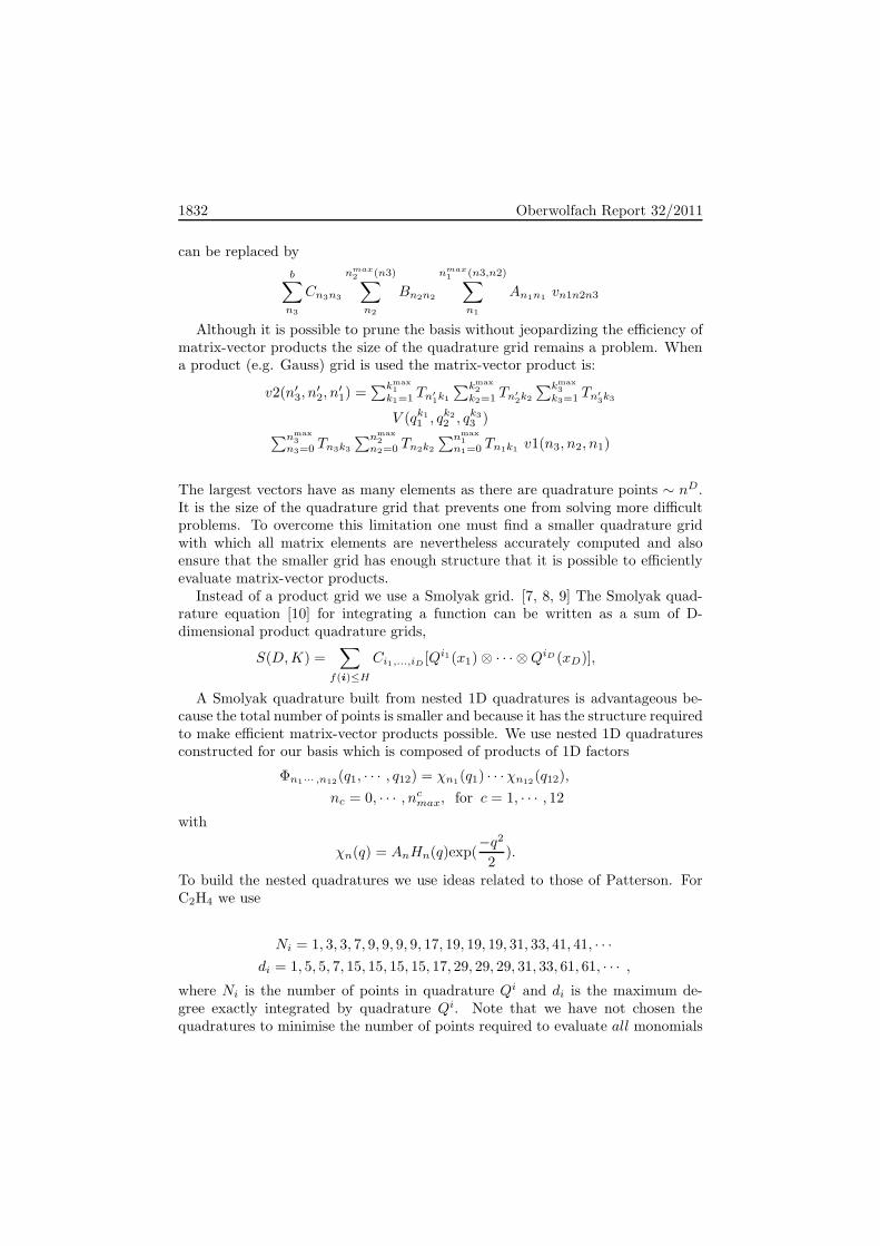
1832 Oberwolfach Report 32/2011
can be replaced by
b∑
n3
Cn3n3
nmax2 (n3)∑
n2
Bn2n2
nmax1 (n3,n2)∑
n1
An1n1 vn1n2n3
Although it is possible to prune the basis without jeopardizing the efficiency ofmatrix-vector products the size of the quadrature grid remains a problem. Whena product (e.g. Gauss) grid is used the matrix-vector product is:
v2(n′3, n
′2, n
′1) =
∑kmax1
k1=1 Tn′
1k1
∑kmax2
k2=1 Tn′
2k2
∑kmax3
k3=1 Tn′
3k3
V (qk11 , qk2
2 , qk33 )
∑nmax3
n3=0 Tn3k3
∑nmax2
n2=0 Tn2k2
∑nmax1
n1=0 Tn1k1 v1(n3, n2, n1)
The largest vectors have as many elements as there are quadrature points ∼ nD.It is the size of the quadrature grid that prevents one from solving more difficultproblems. To overcome this limitation one must find a smaller quadrature gridwith which all matrix elements are nevertheless accurately computed and alsoensure that the smaller grid has enough structure that it is possible to efficientlyevaluate matrix-vector products.
Instead of a product grid we use a Smolyak grid. [7, 8, 9] The Smolyak quad-rature equation [10] for integrating a function can be written as a sum of D-dimensional product quadrature grids,
S(D,K) =∑
f(i)≤H
Ci1,...,iD [Qi1(x1)⊗ · · · ⊗QiD (xD)],
A Smolyak quadrature built from nested 1D quadratures is advantageous be-cause the total number of points is smaller and because it has the structure requiredto make efficient matrix-vector products possible. We use nested 1D quadraturesconstructed for our basis which is composed of products of 1D factors
Φn1··· ,n12(q1, · · · , q12) = χn1(q1) · · ·χn12(q12),
nc = 0, · · · , ncmax, for c = 1, · · · , 12
with
χn(q) = AnHn(q)exp(−q22
).
To build the nested quadratures we use ideas related to those of Patterson. ForC2H4 we use
Ni = 1, 3, 3, 7, 9, 9, 9, 9, 17, 19, 19, 19, 31, 33, 41, 41, · · ·di = 1, 5, 5, 7, 15, 15, 15, 15, 17, 29, 29, 29, 31, 33, 61, 61, · · · ,
where Ni is the number of points in quadrature Qi and di is the maximum de-gree exactly integrated by quadrature Qi. Note that we have not chosen thequadratures to minimise the number of points required to evaluate all monomials

Mathematical Methods in Quantum Chemistry 1833
of degree 2K − 1. Instead, we have chosen to increase the number of importantmonomials, with a subset of the coordinates, for which integrals are exact.
In our calculations we use a KEO in normal coordinates,
T = −1
2
D∑
k
ωk∂2
∂qk2+K .
K is a complicated term whose treatment is presented in reference [9]. The Lanc-zos algorithm is used, without re-orthogonalisation, to compute eigenvalues andeigenvectors.
The hardest part of the calculation is the potential matrix-vector product. ASmolyak grid has fewer points, but the Smolyak quadrature equation (Eq. (1))has a sum over contributing grids (the sum over f(i) ≤ H in Eq. (1)). To reducethe cost of the potential matrix-vector product it is crucial to avoid repeatingthis sum at each Lanczos iteration. This can be done by incorporating the sumover contributions into weights. The Smolyak quadrature of a function f can bewritten,
S(6,K)f(q1, q2, q3, q4, q5, q6)
=∑N1
k1
∑N2
k2
∑N3
k3
∑N4
k4
∑N5
k5
∑N6
k6w(k6, k5, k4, k3, k2, k1)
×f(qk11 , q
k22 , qk3
3 , qk44 , qk5
5 , qk66 ) ,
where kc labels a quadrature point for coordinate c andNc is the maximum numberof points for coordinate qc. N1 is independent of kc 6=1
N1 = N ((H − (D − 1)))
Using the notation Nj = N(j) the other maxima are
Nc = N
(H −
c−1∑
i=1
g(ki)− (D − c))
where c = 2, 3, · · · , and g(k) is the smallest quadrature rule in the sequence ofquadratures that contains point k.
The new weights are,
w(k6, · · · , k1) =∑
f(i)≤H
Ci1,··· ,i6i1wk1 · · · iDwk6 ,
where icwkc is the (1D) weight for the point qkcc ∈ Qic , and iwk = 0 if qk /∈ Qi. In
terms of these weights the potential matrix-vector product is computed by doingsums sequentially,
v2(n′3, n
′2, n
′1) =
∑N1
k1=1 Tn′
1k1
∑N2
k2=1 Tn′
2k2
∑N3
k3=1 Tn′
3k3
w(k3, k2, k1)V (qk11 , qk2
2 , qk33 )
∑nmax3
n3=0 Tn3k3
∑nmax2
n2=0 Tn2k2
∑nmax1
n1=0 Tn1k1
v1(n3, n2, n1) ,

1834 Oberwolfach Report 32/2011
where Tnk = AnHn(qk). Note that by defining new weights that combine theSmolyak coefficients Ci1,··· ,i6 and the icwkc we avoid the need to sum over con-tributing grids at each Lanczos iteration. [7, 8, 9]
In Ref. [9] we present vibrational energy levels of C2H4 computed with a basiswhose size is determined by n1+· · ·+n12 ≤ 11. There are 1.4×10⁶ basis functions.A Smolyak grid with H = 25 with 1.5×10⁸ quadrature points was used. A productGauss grid with comparable accuracy has ∼ 6× 10¹³ points
This work has been supported by the Natural Sciences and Engineering Re-search Council of Canada.
References
[1] S. Carter and N.C. Handy Variational Calculations for triatomic molecules Comput. Phys.Rep. 5 (1986), 115-142
[2] J. C. Light and T. Carrington, Discrete variable representations and their utilization Ad-
vances in Chemical Physics 114 (2000), 263-310[3] M.J. Bramley and T. Carrington A general discrete variable method to calculate vibrational
energy levels of three- and four-atom molecules J. Chem. Phys. 99 (1993) 8519-8541[4] X.-G. Wang and T. Carrington The utility of constraining basis function indices when using
the Lanczos algorithm to calculate vibrational energy levels J. Phys. Chem. 105 (2001)2575-2581
[5] S. Manzhos and T. Carrington, Using neural networks to represent potential surfaces assums of products, J. Chem. Phys. 125 (2006) 194105
[6] Mike Espig, Lars Grasedyck, and Wolfgang Hackbusch Black Box Low Tensor Rank Ap-proximation using Fibre-Crosses Constructive approximation, 30 (2009) 557-597
[7] G. Avila and T. Carrington, Non-product quadrature grids for solving the vibrationalSchrodinger equation , J. Chem. Phys. 131 (2009), 174103
[8] G. Avila and T. Carrington, Using non-product quadrature grids to solve the vibrationalSchrodinger equation in 12D , J. Chem. Phys. 134 (2011), 054126
[9] G. Avila and T. Carrington, Using a pruned basis, a non-product quadrature grid, and theexact Watson normal-coordinate kinetic energy operator to solve the vibrational Schrodingerequation for C2H4 , J. Chem. Phys. in press.
[10] E. Novak and K. Ritter High dimensional integration of smooth functions over cubes Nu-mer. Math. 75, (1996) 79-97
Unique Hartree-Fock Minimizers for Closed Shell Atoms
Fabian Hantsch
(joint work with Marcel Griesemer)
In this talk we discussed the problem of uniqueness of minimizers for the Hartree-Fock functional of atoms. It was shown that the Hartree-Fock ground state isunique provided the number of electrons is of the form N = 2
∑sn=1 n
2, s ∈ N, andthe atomic number Z is sufficiently large compared to N . More specifically, a two-electron atom with atomic number Z ≥ 35 has a unique Hartree-Fock ground stategiven by two orbitals with opposite spins and identical spatial wave functions. Ourresult implies that the General, Unrestricted and Restricted Hartree-Fock (GHF,UHF, RHF) ground states coincide. The fact that this is wrong for N = 2 andsome Z > 1 [2] shows the necessity of some lower bound on Z for the uniqueness

Mathematical Methods in Quantum Chemistry 1835
of the ground state. Our method also applies to Restricted Hartree-Fock theorywhere we can allow for any atom whose electrons are in an arbitrary closed shellconfiguration. We refer to [1] for further details and more results on existence anduniqueness of critical points for both the Hartree-Fock and the Hartree functionals.
References
[1] M. Griesemer, F. Hantsch, Unique Solutions to Hartree-Fock Equations for Closed ShellAtoms, arXiv:1012.5179v1 [math-ph].
[2] Mary Beth Ruskai and Frank H. Stillinger, Binding limit in the Hartree approximation, J.Math. Phys. 25(6):2099–2103, 1984.
QC-DMRG and recent advances in tensor product approximation
Reinhold Schneider
The DMRG algorithm is a well established tool for computing strongly cor-related quantum systems, widely used for lattice spin systems [S]. Presently weconsider its application to the numerical solution of the electronic Schrodingerequation the QC-DMRG (quantum chemistry DMRG) e.g. [LH]. The numeri-cal solution of partial differential equations in d dimensions, d >> 1, is hardlyhempered by the unfavourable scaling O(nd) of traditional approximation meth-ods, often refered to as the curse of dimensionality. Approximation by a sum oftensor products of single variate functions offer an efficient and very flexible toolfor data sparse approximation for high dimensional tensors or high dimensionalfunctions. For convenience of exposition, we will consider a tensor U ∈ Rn1×...×nd
of order (or dimension), as a multivariate function or multi-indexed array, of theform
x 7→ U(x) = U(x1, . . . , xd) : I1 × · · · × Id −→ K , K = R or C
with variables or indices xi from finite index sets Ii := 1, . . . , ni, i ∈ 1, . . . , d,where d ∈ N and n1, . . . , nd. Unfortunately, except the elementary (matrix) cased = 2, the canonical format
U(x1, . . . , xd) =
rc∑
i=1
Ui =
rc∑
i=1
d⊗
ν=1
ui,ν(xν) =
rc∑
i=1
d⊗
ν=1
uν(xν , i) ,
suffers from various shortcomings, making the actual computation of a low-rankapproximation a numerically hazardous task. Nevertheless, it reduces the amountof required data to O(nrcd). This is in contrast the so-called Tucker decompo-sition, In essence, the Tucker format is a subspace approximation. It provides akind of parametrization which is appropriate for optimization and the treatmentdynamical equations. This concept is well estbalished in phyiscs, e.g the MCSCFand MCTHF methods. It has been shown, that the Tucker format provides anembedded manifold. Since the representation of a tensor in the Tucker formatrequires O(rd + dn), n := maxnν : 1 ≤ ν ≤ d, degrees of of freedom (DOF), itdoes not circumvent from the curse of dimensionality. To overcome this dilemma,new formats built on a hierarchical structure for tensor decomposition has been

1836 Oberwolfach Report 32/2011
introduced in [HT]. and [TT]. Where the latter TT format is a special and sim-plest case of the more general hierachical Tucker format in [HT]. Although theseformats have been apparent in various concepts in quantum mechanics, e.g. liketree tensor networks (≃ HT) and matrix product states (≃ TT ), its perspectivefrom mathematics is independent of its application, focusing on issues like approx-imation, existence and stability. A representation of a tensor U ∈ Rn1×···×nd inthe TT tensor format rewrites an order-d tensor in the form
U(x) =
r1∑
k1=1
. . .
rd−1∑
kd−1=1
U1(x1, k1)U2(k1, x2, k2) . . . Ud−1(kd−2, xd−1, kd−1)Ud(kd−1, xd),
where for 2 ≤ i ≤ d− 1, (ki−1, xi, ki) 7→ Ui(ki−1, xi, ki) ∈ Rri−1×ni×ri . RecentlyHackbusch and Falco proved the existence of best approximation, and we haveshown that the TT-format provides an embedded manifold, see e.g [HRS-1] forfurther details. Therefore, the TT format requires only a data complexity of orderO(nr2d), but it is inheriting all stability issues of the Tucker format. The electronicSchrodinger equation, is the basic equation in quantum chemistry It describes thestationary and non-relativistic behavior of an ensemble of N electron exposed toan electric Coulomb field given by fixed nuclei. The electron wave function Ψ obeysthe Pauli antisymmetry principle Since the novel tensor formats are sensitive w.r.t.permutation of variables, we pursue an alternativ way [HRS-1], using the discreteFock space F built by all Slater determinants
ΨSL[k1, . . . , kN ](x1, s1; . . . ;xN , sN ) :=1√N !
det(ϕki(xj , sj))Ni,j=1.
out of a given orthonormal orbital basis set, Xh := span ϕi : i = 1, . . . , d.
F :=
d⊕
N=1
VNFCI =
d⊕
N=1
N∧
i=1
Xh = Ψ : Ψ =∑
µ
cµΨµ .
As standard in FCI computation, a labeling of indices µ ∈ I by an binary stringof length d
e.g.: µ = (0, 0, 1, 1, 0, . . .) =: (µ1, . . . , µi, . . . , µd , µi = 0, 1 ,
• µi = 1 means ϕi is (occupied) in Ψ[. . .].• µi = 0 means ϕi is absend (not occupied) in Ψ[. . .].
yields that the discrete Fock space could be completely parametrized by tensors
F ≃ c : µ 7→ c(µ0, . . . , µd−1) = cµ , µi = 0, 1 =d⊗
i=1
K2 .
Instead of bit manipulations we can reformulate the calculus of second quantization
with creation and annihilation operators a(†)p , ap by simple Kronecker products of
the 2× 2 matrices
A :=
(0 10 0
), AT =
(0 01 0
), S :=
(−1 00 1
), I :=
(1 00 1
).

Mathematical Methods in Quantum Chemistry 1837
One obtains that the discrete creation (annihilation) operators corresponds to
a(†)p ≃ A(T )p := S ⊗ . . .⊗ S ⊗A(T )
(p) ⊗ I ⊗ . . .⊗ I
where A(p) means that A appears on the p-th position in the product. We adherecompletely on the present one-to-one correspondence between the (discrete) Fockspace and the tensor space of corresonding amplitudes, to describe the (discrete)
Hamiltonian H =∑d
p,q=1 hqpA
Tp Aq +
∑dp,q,r,s=1 g
p,qr,sA
Tr A
Ts ApAq and the particle
number operator P =∑d
p,q=1 ATp Aq, where h
qp and gp,qr,s denote the well known
one and two electron integrals,
hpq := 〈ϕq, (−12
∆− Vcore)ϕp〉 , gp,qr,s :=1
2〈ϕr(x, s1)ϕs(y, s2),
ϕp(x, s1)ϕq(y, s2)
|x− y| 〉 .
To obtain the ground state of an N -electron system, we have to take care about re-quired symmetries. We can casted full CI Schrodinger equation into the variationalform [HRS-1] So far, except the full CI approximation, no further approximationhas been applied. Moreover the above representation depends crucuially on thechoice of the underlying basis functions. Due to the combinatorial complexityof FCI computation, further approximations are required. We will focus on ten-sor product approximation by solving the following variational problem along themanifold of TT tensors (or matrix product states) of prescribed rank
U = (U(µ)) = argmin〈HU,U〉 : 〈U,U〉 = 1 , PU = N ,U ∈ Tr .We remark that the crucial parameter, the rank ri, i = 1, . . . , d− 1, is defined bythe rank ri = rank
[U
µi+1,...,µdµ1,...,µi
]of the matricisation or unfolding of the tensor
U(µ1, . . . , µi, µi+1, . . . , µd) ≃ Uµi+1,...,µdµ1,...,µi
.
Separating the complete system into two subsystems systems A, B, built by theorbital basis sets ϕ1 . . . , ϕi and ϕi+1, . . . , ϕd, the above observation impliesthat the TT format or MPS describes the interaction between these two systemsexplicitely. In particular, if both systems are independent, the rank ri = 1, thusproviding size consistency. The above variational problem can be tackled algorith-mitically by an alternating direction approach an alternating linear squares scheme(ALS) . Let us fix all tensors Ui(µi), i ∈ 1, . . . , d\j, except the one for index j.We are going to optimize Uj(kj−1, xj , kj) in an micro-iteration step. We performthis procedure sequentially with j = 1, . . . , d−1, then we repeat the relaxation pro-cedure in the opposite direction. This scheme has the disadvantage that the ranksrj are given a priorily. To adapt the individual ranks rj , we modify the scheme,by concatenating two variables µj , µj+1 into one (µj , µj+1), and searching for anoptimized component W (kj−1, µj , µj+1, kj+1). In a subsequent decimation step,we approximate W(µj , µj+1) = Uj(µj)Vj(µj+1) by low rank, e.g. by means ofSVD, up to a tolerance ǫj. We keep Uj and proceed by computing W(µj+1, µj+2)next. This modified alternating linear scheme (MALS) applied to this problemresembles exactly the DMRG (density matrix renormalization group) method [S]for spin chains.

1838 Oberwolfach Report 32/2011
Summary: The TT format, resp. matrix product states approximates the FullCI solution in a data sparse way. Although it permeates the full CI space, allcomputations can be performed within polynomial complexity. The electron den-sity as well as reduced one- and two- body density matrices can be computedin polynomial cost. It provides inside in particular separations into subsystemsand its entanglement. This make this approach atractive for the computationof stronlgy correlated systems, where Coupled Cluster methods are failing. Theapproximation depends crucially on the choice of orbital basis functions and itsordering.
References
[LH] O Legeza, J. Roder, B. A. Hess, Controlling the accuracy of the density matrix renormal-
ization group method: The Dynamical Block State Selection approach, Phys. Rv. B 67,125114 (2003).
[HT] W. Hackbusch, S. Kuhn, A new scheme for the tensor representation, Preprint 2, MPIMIS, 2009.
[HRS-1] S. Holtz, T. Rohwedder and R. Schneider, The manifold of tensors of fixed TT-rank,Preprint SPP 1324 (2010)
[HRS-2] S. Holtz, T. Rohwedder and R. Schneider, A relaxation scheme for optimization in theTT- tensor format - DMRG , Preprint SPP 1324 (2010)
[TT] I. Oseledets, E. E. Tyrtyshnikov, Breaking the curse of dimensionality , or how to use SVDin many dimensions, SIAM J. Sci. Comput., Vol.31 (5), 2009, 3744–3759.
[S] U. Schollwock, The density-matrix renormalization group, Rev. Mod. Phys. 77 1, p. 259,2005
Projected quasiparticle theory for molecular electronic structure
Gustavo E. Scuseria
(joint work with Carlos A. Jimenez-Hoyos, Thomas M. Henderson, KousikSamanta, Jason K. Ellis)
We derive and implement symmetry-projected Hartree-Fock-Bogoliubov (HFB)equations and apply them to the molecular electronic structure problem. Allsymmetries (particle number, spin, spatial, and complex conjugation) are deliber-ately broken and restored in a self-consistent variation-after-projection approach.We show that the resulting method yields a comprehensive black-box treatmentof strong correlations with effective one-electron (mean-field) computational cost.The ensuing wave function is of multireference character and permeates the entireHilbert space of the problem. The energy expression is different from regular HFBtheory but remains a functional of an independent quasiparticle density matrix.All reduced density matrices are expressible as an integration of transition den-sity matrices over a gauge grid. We present several proof-of-principle examplesdemonstrating the compelling power of projected quasiparticle theory for elec-tronic structure theory.
There are many mathematical aspects of this work that I discussed. Theseinclude but are not limited to the role of antiunitary symmetries that do not carry

Mathematical Methods in Quantum Chemistry 1839
“good” quantum numbers and the importance of coherent states in symmetrybreaking and restoration.
References
[1] Gustavo E. Scuseria, Carlos A. Jimenez-Hoyos, Thomas M. Henderson, Kousik Samanta,Jason K. Ellis, Projected quasiparticle theory for molecular electronic structure, J. Chem.Phys. 135 (2011), 124108.
Reporter: Christian Mendl

1840 Oberwolfach Report 32/2011
Participants
Prof. Dr. Ali Alavi
Department of ChemistryUniversity of CambridgeLensfield RoadGB-Cambridge CB2 1EW
Dr. Alexander A. Auer
Max-Planck-Institut furEisenforschung GmbHMax-Planck-Str. 140237 Dusseldorf
Prof. Dr. Volker Bach
Institut fur Algebra u. AnalysisTU BraunschweigPockelsstr. 1438106 Braunschweig
Udo Benedikt
Max-Planck-Institut furEisenforschung GmbHMax-Planck-Str. 140237 Dusseldorf
Dr. Volker Betz
Mathematics InstituteUniversity of WarwickGibbet Hill RoadGB-Coventry CV4 7AL
Prof. Dr. Eric Cances
CERMICS - ENPCCite Descartes, Champs-sur-Marne6 et 8 avenue Blaise PascalF-77455 Marne La Vallee Cedex 2
Prof. Dr. Tucker Carrington
Chemistry DepartmentQueen’s UniversityKingston, Ontario K7L 3N6CANADA
Prof. Dr. Isabelle Catto
CEREMADEUniversite Paris DauphinePlace du Marechal de Lattre deTassignyF-75775 Paris Cedex 16
Prof. Dr. Jerzy Cioslowski
Institute of PhysicsUniversity of Szczecinul. Wielkopolska 1570-451 SzczecinPOLAND
Dr. Luigi Delle Site
Max-Planck Institut fur Polymer-forschungAckermannweg 1055128 Mainz
Virginie Ehrlacher
CERMICS - ENPCCite Descartes, Champs-sur-Marne6 et 8 avenue Blaise PascalF-77455 Marne La Vallee Cedex 2
Dr. Mike Espig
Max-Planck-Institut fur Mathematikin den NaturwissenschaftenInselstr. 22 - 2604103 Leipzig
Dr. Heinz-Jurgen Flad
Fakultat II - Institut fur MathematikTechnische Universitat BerlinSekr. MA 5-3Straße des 17. Juni 13610623 Berlin

Mathematical Methods in Quantum Chemistry 1841
Prof. Dr. Gero Friesecke
Fakultat fur MathematikTechnische Universitat MunchenBoltzmannstr. 385748 Garching bei Munchen
Prof. Dr. Carlos J. Garcia-Cervera
Department of MathematicsUniversity of California atSanta BarbaraSouth HallSanta Barbara , CA 93106USA
Prof. Dr. Peter Gill
Research School of ChemistryAustralian National UniversityCanberra ACT 0200AUSTRALIA
Dr. Ben Goddard
Department of Chemical EngineeringImperial College LondonSouth Kensington CampusGB-London SW7 2AZ
Prof. Dr. Dr.h.c. Wolfgang Hack-
busch
Max-Planck-Institut fur Mathematikin den NaturwissenschaftenInselstr. 22 - 2604103 Leipzig
Prof. Dr. George A. Hagedorn
Department of MathematicsVirginia TechBlacksburg , VA 24061-0123USA
Dr. Jan Hamaekers
Fraunhofer-Institut furAlgorithmen und WissenschaftlichesRechnen (SCAI)Schloss Birlinghoven53754 Sankt Augustin
Stefan Handschuh
Max-Planck-Institut fur Mathematikin den NaturwissenschaftenInselstr. 22 - 2604103 Leipzig
Fabian Hantsch
Fachbereich MathematikUniversitat StuttgartPfaffenwaldring 5770569 Stuttgart
Frederik Heber
Institut fur Numerische SimulationUniversitat BonnWegelerstr.653115 Bonn
Stefan Kuhn
Max-Planck-Institut fur Mathematikin den NaturwissenschaftenInselstr. 22 - 2604103 Leipzig
Prof. Dr. Werner Kutzelnigg
Lehrstuhl fur Theoretische ChemieRuhr-Universitat Bochum44780 Bochum
Salma Lahbabi
CERMICS - ENPCCite Descartes, Champs-sur-Marne6 et 8 avenue Blaise PascalF-77455 Marne La Vallee Cedex 2
Robert Lang
Physik Department T 39TU MunchenJames-Franck-Str. 185747 Garching bei Munchen

1842 Oberwolfach Report 32/2011
Prof. Dr. Caroline Lasser
Zentrum MathematikTechnische Universitat MunchenBoltzmannstr. 385747 Garching bei Munchen
Dr. Mathieu Lewin
Departement de MathematiquesUniversite de Cergy-PontoiseSite Saint-Martin, BP 2222, avenue Adolphe ChauvinF-95302 Cergy-Pontoise Cedex
Lin Lin
Department of MathematicsPrinceton University609 Fine HallWashington RoadPrinceton , NJ 08544USA
Dr. Pierre-Francois Loos
Research School of ChemistryAustralian National UniversityCanberra ACT 0200AUSTRALIA
Dr. Jianfeng Lu
New York UniversityCourant Institute of MathematicalSciences251 Mercer StreetNew York , NY 10012USA
Falko Marquardt
Zentrum MathematikTU MunchenBoltzmannstr. 385748 Garching b. Munchen
Christian Mendl
Zentrum MathematikTU MunchenBoltzmannstr. 385748 Garching b. Munchen
Prof. Dr. Peter Pulay
Department of Chemistry & BiochemistryUniversity of Arkansas119 Chemistry BuildingFayetteville , AR 72701USA
Thorsten Rohwedder
Fakultat II - Institut fur MathematikTechnische Universitat BerlinSekr. MA 5-3Straße des 17. Juni 13610623 Berlin
Prof. Dr. Andreas Savin
Laboratoire de Chimie TheoriqueCNRS UMR 7616Universite de Pierre et Marie CurieCase 137, 4 place JussieuF-75252 Paris Cedex 05
Prof. Dr. Reinhold Schneider
Fakultat II - Institut fur MathematikTechnische Universitat BerlinSekr. MA 5-3Straße des 17. Juni 13610623 Berlin
Prof. Dr. Gustavo E. Scuseria
Department of ChemistryRice University6100 Main StreetHouston TX 77005-1892USA
Prof. Dr. Heinz Siedentop
Mathematisches InstitutLudwig-Maximilians-UniversitatMunchenTheresienstr. 3980333 Munchen

Mathematical Methods in Quantum Chemistry 1843
Prof. Dr. Thomas Sorensen
Mathematisches InstitutLudwig-Maximilians-UniversitatMunchenTheresienstr. 3980333 Munchen
Dr. Alex Thom
Imperial College of Science, Technologyand MedicineDepartment of ChemistryExhibition RoadGB-London SW7 2AZ
Dr. Saber Trabelsi
CEREMADEUniversite Paris DauphinePlace du Marechal de Lattre deTassignyF-75775 Paris Cedex 16
Andre Uschmajew
Institut fur MathematikTechnische Universitat BerlinStraße des 17. Juni 13610623 Berlin
Prof. Dr. Harry Yserentant
Institut fur MathematikTechnische Universitat BerlinStraße des 17. Juni 13610623 Berlin
