mathematical modeling & simulation, math...
TRANSCRIPT
Continuous Mathematical Models: Second Order Models – Mechanical & Electrical Systems
Mathematical Modeling &
Simulation, MATH 463
Dr. Alam Z M Barkat Ali First Order Models, MATH 463 1
Instuctor: Dr. Samy MZIOUslides from Dr. Alam Z M Barkat Ali

Second Order ODE Based Models• A linear model based on a second order ODE has the following
general form:
where a(t), b(t), c(t), f(t) are known functions and , areconstants. The function f(t) is called input, driving function, orforcing function.
• The model is homogenous if f(t) = 0, otherwise it is non-homogeneous. A solution y(t) of the differential equation thatsatisfies initial conditions is called output or response of the systemrepresented by the model.
• Second order models have many important applications in practicalworld. We will consider some very simple dynamical systems inwhich mathematical model is a second order ordinary differentialequation, with a(t), b(t), c(t) being constants.
---------------------------------------------------------------------------------------Dr. Alam Z M Barkat Ali First Order Models, MATH 463 2
)0( ,)0( ),()()()(2
2
yytfytcdt
dytb
dt
ydta

Spring-Mass System: Hooke’s Law• Suppose a flexible spring of length is
suspended vertically from a rigid supportand a body of mass m is attached to its freeend. The spring stretches by an amount s &attains an equilibrium position.
• According to Hooke’s law the spring exertsa restoring force Fr on the body, which isopposite to the direction of stretch & isproportional to the amount of elongation,i.e.
Fr s Fr = - k s
where k is constant of proportionality,called spring constant.
• At equilibrium position weight mg of thebody will balance the restoring force, i.e.
mg = k s mg – k s =0Dr. Alam Z M Barkat Ali First Order Models, MATH 463 3
------------------------------------------------------------------------------------------------------------
l

Spring-Mass System: Free undamped Motion• Forces acting on the body are Fr & its weight
mg. If the body attached to the spring isnow displaced by an amount from theequilibrium position, restoring force of thespring becomes
• We assume that, other than Fr , there are noresistive forces acting on the system. Thus,total force F on the body is:
• By the Newton’s second law we can write
Hence, equation of motion of the system is
Dr. Alam Z M Barkat Ali 4First Order Models, MATH 463
y
).( sykFr
kykyksmgyskmgF )(
2
2
dt
ydmF
ydt
xdy
m
k
dt
ydyk
dt
ydm 2
2
2
2
2
2
2
mkydt
yd/ , 22
2
2
-------------------------------------------------------------------------------------------------------------
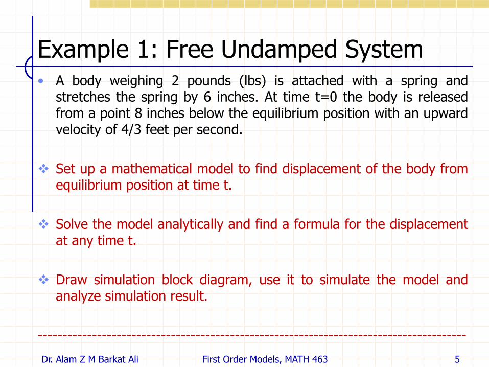
Example 1: Free Undamped System• A body weighing 2 pounds (lbs) is attached with a spring and
stretches the spring by 6 inches. At time t=0 the body is releasedfrom a point 8 inches below the equilibrium position with an upwardvelocity of 4/3 feet per second.
Set up a mathematical model to find displacement of the body fromequilibrium position at time t.
Solve the model analytically and find a formula for the displacementat any time t.
Draw simulation block diagram, use it to simulate the model andanalyze simulation result.
---------------------------------------------------------------------------------------
Dr. Alam Z M Barkat Ali First Order Models, MATH 463 5
Example 1: Mathematical Model
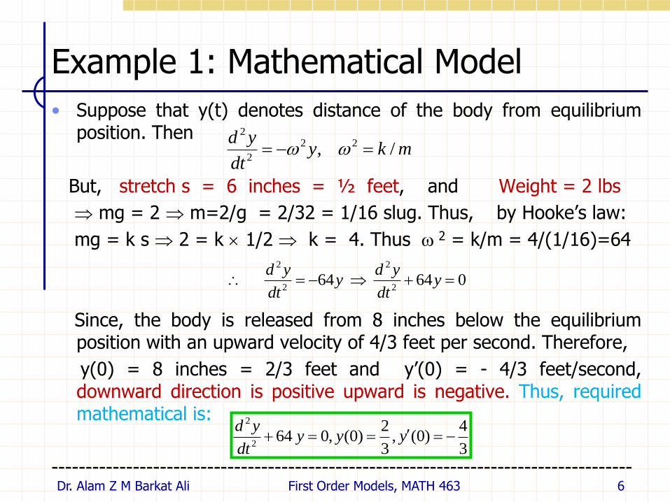
• Suppose that y(t) denotes distance of the body from equilibriumposition. Then
But, stretch s = 6 inches = ½ feet, and Weight = 2 lbs
mg = 2 m=2/g = 2/32 = 1/16 slug. Thus, by Hooke’s law:
mg = k s 2 = k 1/2 k = 4. Thus 2 = k/m = 4/(1/16)=64
Since, the body is released from 8 inches below the equilibriumposition with an upward velocity of 4/3 feet per second. Therefore,
y(0) = 8 inches = 2/3 feet and y’(0) = - 4/3 feet/second,downward direction is positive upward is negative. Thus, requiredmathematical is:
--------------------------------------------------------------------------------------Dr. Alam Z M Barkat Ali First Order Models, MATH 463 6
mkydt
yd/ , 22
2
2
064 64 2
2
2
2
ydt
ydy
dt
yd
3
4)0(,
3
2)0(,0 64
2
2
yyydt
yd

Example 1: Analytical Solution
•
------------------------------------------------------------------------Dr. Alam Z M Barkat Ali First Order Models, MATH 463 7
)8sin(6
1)8cos(
3
2)( ttty
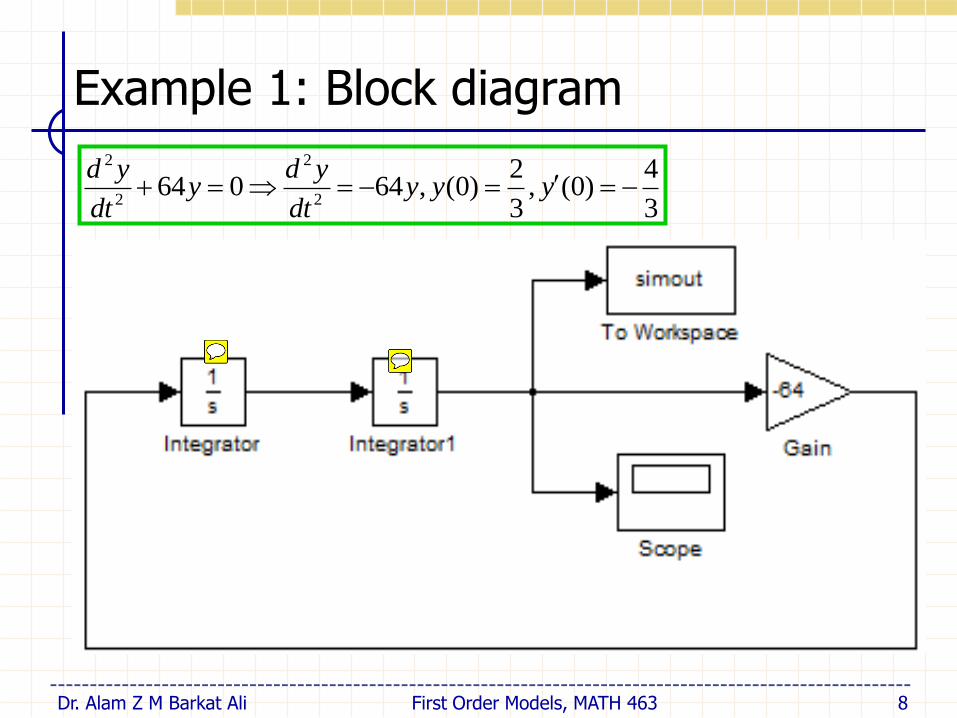
Example 1: Block diagram
Dr. Alam Z M Barkat Ali First Order Models, MATH 463 8
3
4)0(,
3
2)0(,64064
2
2
2
2
yyydt
ydy
dt
yd
------------------------------------------------------------------------------------------------------------

Example 1: Simulation Result
•
------------------------------------------------------------------------Dr. Alam Z M Barkat Ali First Order Models, MATH 463 9
From this figure we see simple harmonic motion about equilibrium position
in the absence of any resistive force and oscillation do not approach to zero.
Spring-Mass System: Free damped Motion
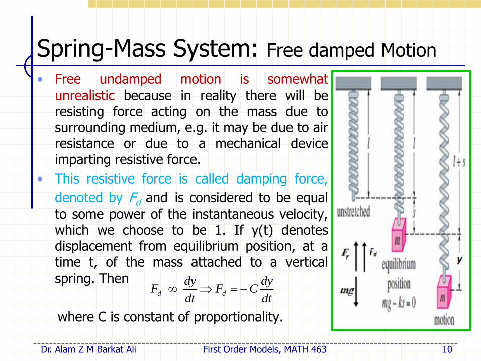
• Free undamped motion is somewhatunrealistic because in reality there will beresisting force acting on the mass due tosurrounding medium, e.g. it may be due to airresistance or due to a mechanical deviceimparting resistive force.
• This resistive force is called damping force,
denoted by Fd and is considered to be equal
to some power of the instantaneous velocity,which we choose to be 1. If y(t) denotesdisplacement from equilibrium position, at atime t, of the mass attached to a verticalspring. Then
where C is constant of proportionality.
Dr. Alam Z M Barkat Ali First Order Models, MATH 463 10
dt
dyCF
dt
dyF dd
----------------------------------------------------------------------------------------------------------
Spring-Mass System: Free damped Motion
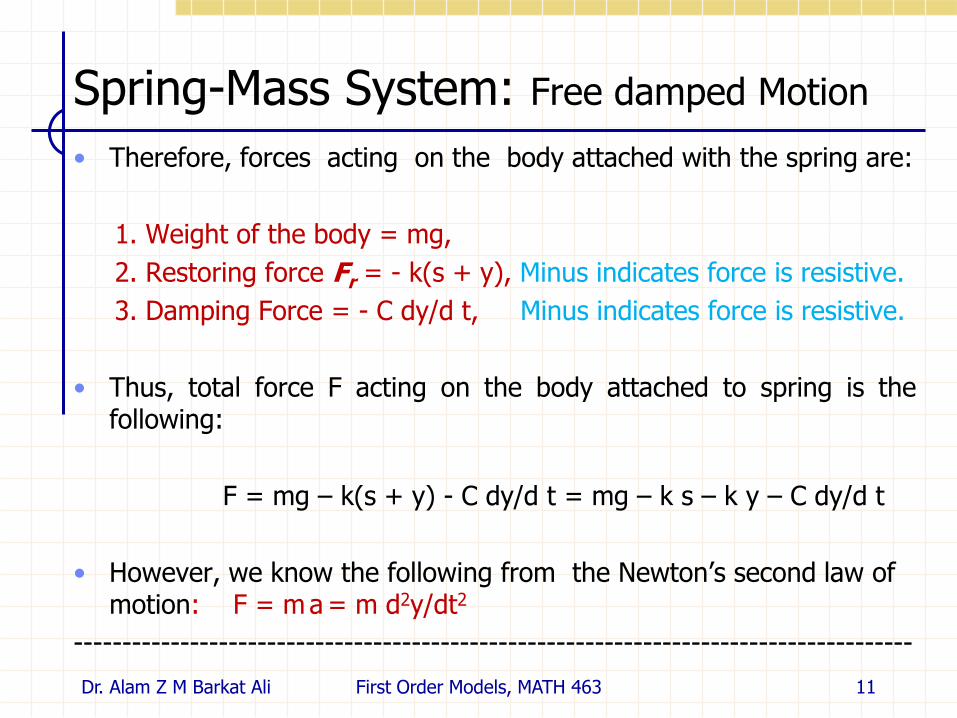
• Therefore, forces acting on the body attached with the spring are:
1. Weight of the body = mg,
2. Restoring force Fr = - k(s + y), Minus indicates force is resistive.
3. Damping Force = - C dy/d t, Minus indicates force is resistive.
• Thus, total force F acting on the body attached to spring is thefollowing:
F = mg – k(s + y) - C dy/d t = mg – k s – k y – C dy/d t
• However, we know the following from the Newton’s second law of motion: F = m a = m d2y/dt2
---------------------------------------------------------------------------------------
Dr. Alam Z M Barkat Ali First Order Models, MATH 463 11

Spring-Mass System: Free damped Motion
• Hence, making use of the last two equations, we can write thefollowing
where 2= C/m and 2 = k/m.
• If the mass attached to spring is released from a point at a distanceof units from equilibrium position with a velocity units persecond. Then, y(0)= and y’(0)=. Hence, equation of motion ofthe system is the following:
---------------------------------------------------------------------------------------Dr. Alam Z M Barkat Ali First Order Models, MATH 463 12
02 2
2
2
2
2
ydt
dy
dt
yd
dt
dy
m
Cy
m
k
dt
yd
)0( ,)0( ,02 2
2
2
yyydt
dy
dt
yd
dt
dyCky
dt
dyCkyksmg
dt
ydm
2
2
Spring-Mass System: Free damped Motion
•
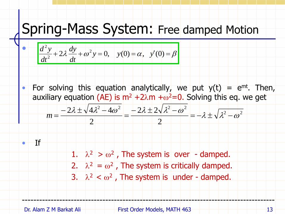
• For solving this equation analytically, we put y(t) = emt. Then,auxiliary equation (AE) is m2 +2m +2=0. Solving this eq. we get
• If
1. 2 > 2 , The system is over - damped.
2. 2 = 2 , The system is critically damped.
3. 2 < 2 , The system is under - damped.
----------------------------------------------------------------------------------------Dr. Alam Z M Barkat Ali First Order Models, MATH 463 13
)0( ,)0( ,02 2
2
2
yyydt
dy
dt
yd
222222
2
22
2
442
m

Example 2: Free (Over) damped motion• Suppose a body weighing 32 lbs stretches a spring by 32 feet.
Assuming that a damping force numerically equal to 3 times theinstantaneous velocity acts on the system. At t = 0 the mass isreleased from a point 10 feet below the equilibrium position fromrest.
Set up a mathematical model to find displacement of the body fromequilibrium position at time t.
Solve the model analytically and find a formula for the displacementat any time t.
Draw simulation block diagram, use it to simulate the model andanalyze simulation result.
---------------------------------------------------------------------------------------
Dr. Alam Z M Barkat Ali First Order Models, MATH 463 14

Example 2: Mathematical Model
• Suppose that y(t) denotes distance of the body from equilibriumposition. Then
But, stretch s = 32 feet, and Weight of the body = 32 lbs.
mg = 32 m=32/g = 32/32 = 1 slug. Thus, by Hooke’s law:
mg = k s 32 = k 32 k = 1. Thus 2 = k/m = 1/1 = 1.Damping Force = - 3(instantaneous vel.) C = 3 2=C/m = 3
Since, the body is released from 10 feet below the equilibriumposition from rest. Therefore, y(0) = 10 feet and y’(0) = 0feet/second, downward direction is positive upward is negative.Thus, required math model is:
---------------------------------------------------------------------------------------Dr. Alam Z M Barkat Ali First Order Models, MATH 463 15
mkmCydt
dy
dt
yd/ ,/2 ,2 22
2
2
03 3 2
2
2
2
ydt
dy
dt
ydy
dt
dy
dt
yd
0)0(,10)0(,0 32
2
yyydt
dy
dt
yd
Example 2: Analytical Solution
•
------------------------------------------------------------------------Dr. Alam Z M Barkat Ali First Order Models, MATH 463 16

Example 2: Block diagram
•
------------------------------------------------------------------------Dr. Alam Z M Barkat Ali First Order Models, MATH 463 17
0)0(,10)0( , 30 32
2
2
2
yyydt
dy
dt
ydy
dt
dy
dt
yd

Example 2: Simulation Result
•
------------------------------------------------------------------------Dr. Alam Z M Barkat Ali First Order Models, MATH 463 18
We see that the initial displacement (downward) of 10 feet decreases and
becomes zero ultimately. This is expected because of the presence of
resistive forces and no driving force.
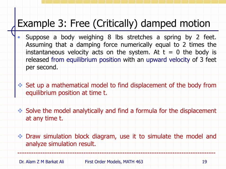
Example 3: Free (Critically) damped motion
• Suppose a body weighing 8 lbs stretches a spring by 2 feet.Assuming that a damping force numerically equal to 2 times theinstantaneous velocity acts on the system. At t = 0 the body isreleased from equilibrium position with an upward velocity of 3 feetper second.
Set up a mathematical model to find displacement of the body fromequilibrium position at time t.
Solve the model analytically and find a formula for the displacementat any time t.
Draw simulation block diagram, use it to simulate the model andanalyze simulation result.
---------------------------------------------------------------------------------------
Dr. Alam Z M Barkat Ali First Order Models, MATH 463 19
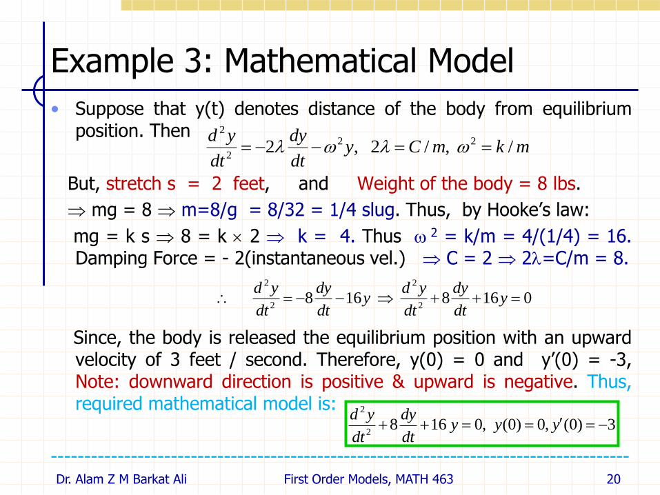
Example 3: Mathematical Model
• Suppose that y(t) denotes distance of the body from equilibriumposition. Then
But, stretch s = 2 feet, and Weight of the body = 8 lbs.
mg = 8 m=8/g = 8/32 = 1/4 slug. Thus, by Hooke’s law:
mg = k s 8 = k 2 k = 4. Thus 2 = k/m = 4/(1/4) = 16.Damping Force = - 2(instantaneous vel.) C = 2 2=C/m = 8.
Since, the body is released the equilibrium position with an upwardvelocity of 3 feet / second. Therefore, y(0) = 0 and y’(0) = -3,Note: downward direction is positive & upward is negative. Thus,required mathematical model is:
---------------------------------------------------------------------------------------Dr. Alam Z M Barkat Ali First Order Models, MATH 463 20
mkmCydt
dy
dt
yd/ ,/2 ,2 22
2
2
0168 168 2
2
2
2
ydt
dy
dt
ydy
dt
dy
dt
yd
3)0(,0)0( ,0 1682
2
yyydt
dy
dt
yd

Example 3: Analytical Solution
•
----------------------------------------------------------------------Dr. Alam Z M Barkat Ali First Order Models, MATH 463 21
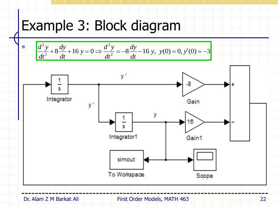
Example 3: Block diagram
•
-------------------------------------------------------------------------Dr. Alam Z M Barkat Ali First Order Models, MATH 463 22
3)0(,0)0( , 1680 1682
2
2
2
yyydt
dy
dt
ydy
dt
dy
dt
yd
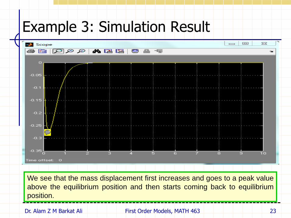
Example 3: Simulation Result
•
-------------------------------------------------------------------------Dr. Alam Z M Barkat Ali First Order Models, MATH 463 23
We see that the mass displacement first increases and goes to a peak value
above the equilibrium position and then starts coming back to equilibrium
position.

Example 4: Free (Under) damped Motion
• Suppose a body weighing 16 lbs is attached to a 5 feet long spring.At equilibrium position the spring measures 8.2 feet. Assume thatthe surrounding medium offers a resistance (damping force) tomotion of the system that is numerically equal to the instantaneousvelocity. At t = 0 the body is released from rest at a point 2 feetabove the equilibrium position.
Set up a mathematical model to find displacement of the body fromequilibrium position at time t.
Solve the model analytically and find a formula for the displacementat any time t.
Draw simulation block diagram, use it to simulate the model andanalyze simulation result.
---------------------------------------------------------------------------------------Dr. Alam Z M Barkat Ali First Order Models, MATH 463 24
Example 4: Mathematical Model
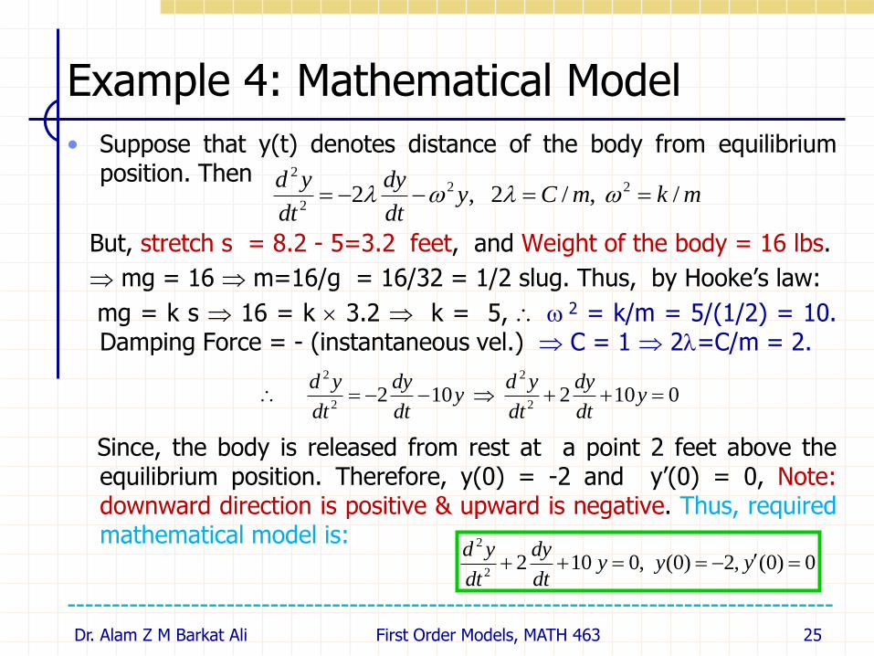
• Suppose that y(t) denotes distance of the body from equilibriumposition. Then
But, stretch s = 8.2 - 5=3.2 feet, and Weight of the body = 16 lbs.
mg = 16 m=16/g = 16/32 = 1/2 slug. Thus, by Hooke’s law:
mg = k s 16 = k 3.2 k = 5, 2 = k/m = 5/(1/2) = 10.Damping Force = - (instantaneous vel.) C = 1 2=C/m = 2.
Since, the body is released from rest at a point 2 feet above theequilibrium position. Therefore, y(0) = -2 and y’(0) = 0, Note:downward direction is positive & upward is negative. Thus, requiredmathematical model is:
---------------------------------------------------------------------------------------Dr. Alam Z M Barkat Ali First Order Models, MATH 463 25
mkmCydt
dy
dt
yd/ ,/2 ,2 22
2
2
0102 102 2
2
2
2
ydt
dy
dt
ydy
dt
dy
dt
yd
0)0(,2)0( ,0 1022
2
yyydt
dy
dt
yd

Example 4: Analytical Solution
•
------------------------------------------------------------------------Dr. Alam Z M Barkat Ali First Order Models, MATH 463 26
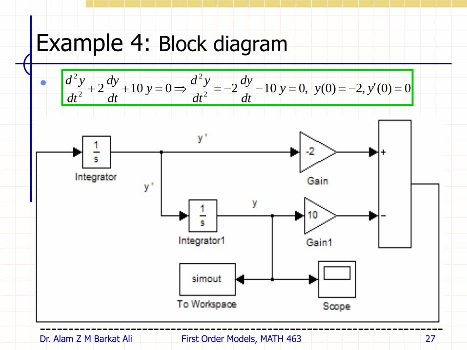
Example 4: Block diagram
•
-----------------------------------------------------------------------Dr. Alam Z M Barkat Ali First Order Models, MATH 463 27
0)0(,2)0( ,0 1020 1022
2
2
2
yyydt
dy
dt
ydy
dt
dy
dt
yd
Example 4: Simulation Result
•
-----------------------------------------------------------------------Dr. Alam Z M Barkat Ali First Order Models, MATH 463 28
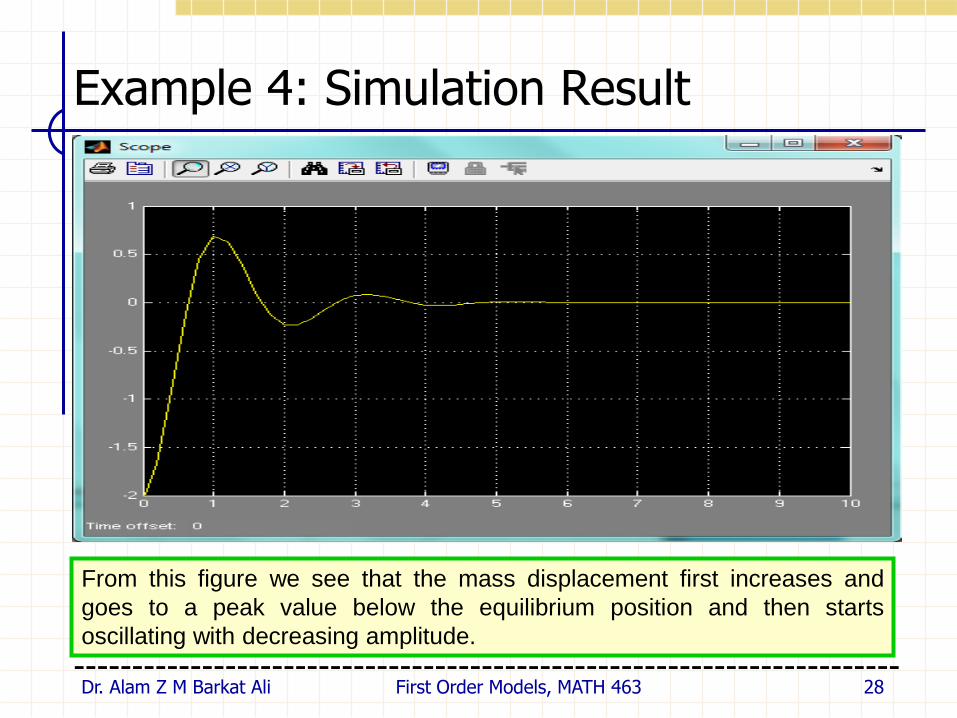
From this figure we see that the mass displacement first increases and
goes to a peak value below the equilibrium position and then starts
oscillating with decreasing amplitude.
Spring-Mass System: Driven Motion
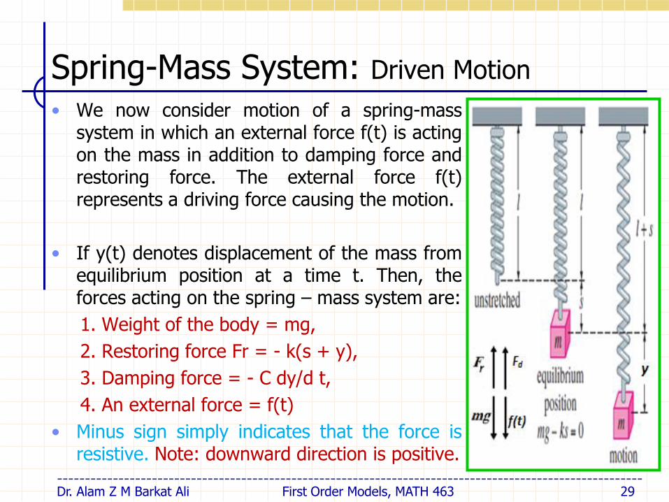
• We now consider motion of a spring-masssystem in which an external force f(t) is actingon the mass in addition to damping force andrestoring force. The external force f(t)represents a driving force causing the motion.
• If y(t) denotes displacement of the mass fromequilibrium position at a time t. Then, theforces acting on the spring – mass system are:
1. Weight of the body = mg,
2. Restoring force Fr = - k(s + y),
3. Damping force = - C dy/d t,
4. An external force = f(t)
• Minus sign simply indicates that the force isresistive. Note: downward direction is positive.
Dr. Alam Z M Barkat Ali First Order Models, MATH 463 29---------------------------------------------------------------------------------------------------------
Spring-Mass System: Driven Motion
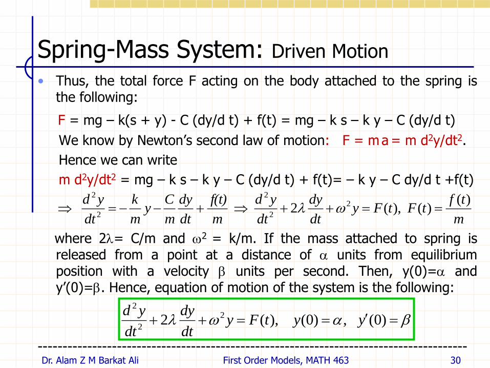
• Thus, the total force F acting on the body attached to the spring isthe following:
F = mg – k(s + y) - C (dy/d t) + f(t) = mg – k s – k y – C (dy/d t)
We know by Newton’s second law of motion: F = ma = m d2y/dt2.
Hence we can write
m d2y/dt2 = mg – k s – k y – C (dy/d t) + f(t)= – k y – C dy/d t +f(t)
where 2= C/m and 2 = k/m. If the mass attached to spring isreleased from a point at a distance of units from equilibriumposition with a velocity units per second. Then, y(0)= andy’(0)=. Hence, equation of motion of the system is the following:
---------------------------------------------------------------------------------------Dr. Alam Z M Barkat Ali First Order Models, MATH 463 30
m
tftFtFy
dt
dy
dt
yd
m
f(t)
dt
dy
m
Cy
m
k
dt
yd )()( ),(2 2
2
2
2
2
)0( ,)0( ),(2 2
2
2
yytFydt
dy
dt
yd
Example 5: Damped Driven Motion
• Suppose a body weighing 6.4 lbs attached to a spring stretches it by3.2 feet. Assume that damping force, numerically equal to 1.2 timesthe instantaneous velocity acts on the mass. In addition an externalforce f(t)=5 co s ( 4 t ) is being applied to the system. At t = 0 thebody is released from rest at a point 0.5 feet below the equilibriumposition.
Set up a mathematical model to find displacement of the body fromequilibrium position at time t.
Solve the model analytically and find a formula for the displacementat any time t.
Draw simulation block diagram, use it to simulate the model andanalyze simulation result.
---------------------------------------------------------------------------------------Dr. Alam Z M Barkat Ali First Order Models, MATH 463 31

Example 5: Mathematical Model
• Suppose y(t) denotes distance of the body from equilibrium position.Then
But, f(t) = 5 co s ( 4 t ) , stretch s = 3.2 ft, and weight = 6.4 lbs.
mg = 6.4 m=6.4/g = 6.4/32 = 1/5 slug. Thus, by Hooke’s law:
mg = k s 6.4 = k 3.2 k = 2, 2 = k/m = 2/(1/5) = 10.Damping Force =-1.2(instantaneous vel.) C = 1.2 2=C/m = 6.
Since, the body is released from rest at a point 0.5 feet below theequilibrium position. Therefore, y(0) = -2 and y’(0) = 0, Note:downward direction is positive & upward is negative. Thus, requiredmathematical model is:
---------------------------------------------------------------------------------------Dr. Alam Z M Barkat Ali First Order Models, MATH 463 32
m
tftF
m
k
m
CtFy
dt
dy
dt
yd )()( , ,2 ),(2 22
2
2
tm
tftFtFy
dt
dy
dt
ydtFy
dt
dy
dt
yd4cos25
)()( ),(106 )(106
2
2
2
2
0)0(,2
1)0( ,4cos25 106
2
2
yytydt
dy
dt
yd

Example 5: Analytical Solution
•
------------------------------------------------------------------------Dr. Alam Z M Barkat Ali First Order Models, MATH 463 33

Example 5: Block diagram
•
------------------------------------------------------------------------Dr. Alam Z M Barkat Ali First Order Models, MATH 463 34
0)0(,2
1)0( ,4cos25 1064cos25 106
2
2
2
2
yytydt
dy
dt
ydty
dt
dy
dt
yd
Example 5: Simulation Result
------------------------------------------------------------------------Dr. Alam Z M Barkat Ali First Order Models, MATH 463 35
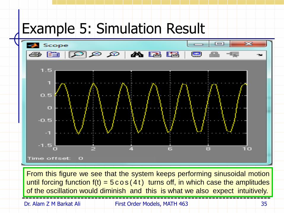
From this figure we see that the system keeps performing sinusoidal motion
until forcing function f(t) = 5 c o s ( 4 t ) turns off, in which case the amplitudes
of the oscillation would diminish and this is what we also expect intuitively.
Electrical Systems: LRC Series Circuits
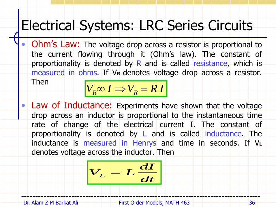
• Ohm’s Law: The voltage drop across a resistor is proportional to
the current flowing through it (Ohm’s law). The constant ofproportionality is denoted by R and is called resistance, which ismeasured in ohms. If VR denotes voltage drop across a resistor.Then
• Law of Inductance: Experiments have shown that the voltage
drop across an inductor is proportional to the instantaneous timerate of change of the electrical current I. The constant ofproportionality is denoted by L and is called inductance. Theinductance is measured in Henrys and time in seconds. If VLdenotes voltage across the inductor. Then
--------------------------------------------------------------------------------------
IRVIV RR
dt
dILVL
Dr. Alam Z M Barkat Ali 36First Order Models, MATH 463
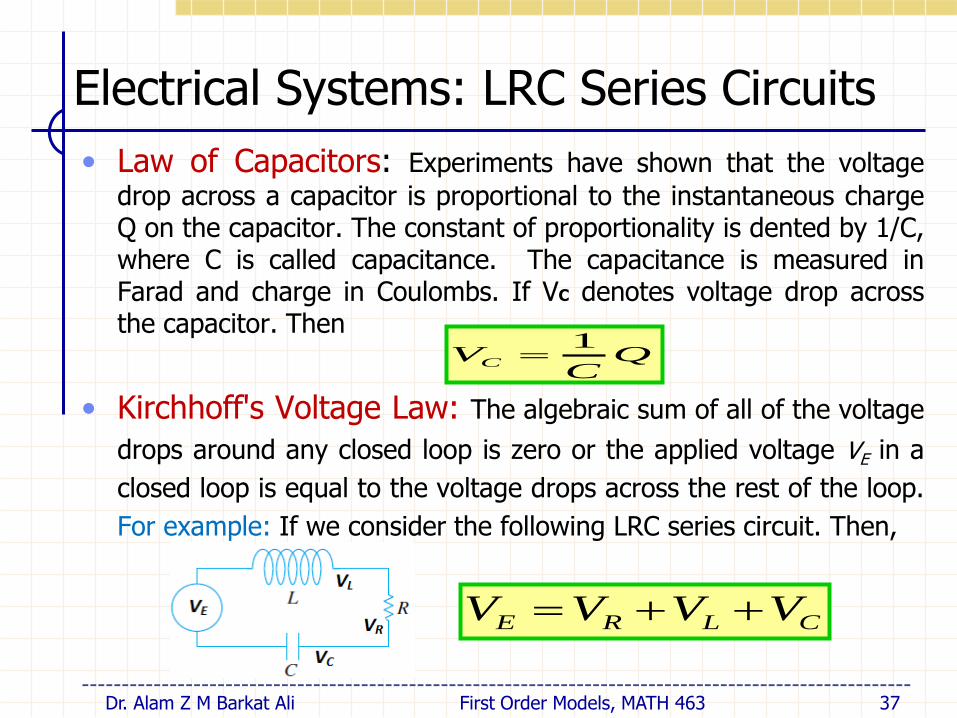
• Law of Capacitors: Experiments have shown that the voltage
drop across a capacitor is proportional to the instantaneous chargeQ on the capacitor. The constant of proportionality is dented by 1/C,where C is called capacitance. The capacitance is measured inFarad and charge in Coulombs. If VC denotes voltage drop acrossthe capacitor. Then
• Kirchhoff's Voltage Law: The algebraic sum of all of the voltage
drops around any closed loop is zero or the applied voltage VE in a
closed loop is equal to the voltage drops across the rest of the loop.
For example: If we consider the following LRC series circuit. Then,
Electrical Systems: LRC Series Circuits
QC
VC
1
Dr. Alam Z M Barkat Ali 37First Order Models, MATH 463
CLRE VVVV
--------------------------------------------------------------------------------------------------------

Electrical Systems: LRC Series Circuits
• Suppose an E(t) volt battery is connected to the following LRCseries electrical circuit and I(t) denotes current in circuit & q(t)charge on capacitor at a time t.
• By using the Kirchhoff’s voltage, we can write the followingequation:
but the charge q(t) and the current are related by relation:
If initial charge on the capacitor is q0 and electric current in circuitis I0 . Then, q(0) = and q’(0) = serve as the initial conditions.
---------------------------------------------------------------------------------------Dr. Alam Z M Barkat Ali First Order Models, MATH 463 38
EECRL VqC
RIdt
dILVVVV
1
dt
dqtI )(
(1) 1
2
2
EVqCdt
dqR
dt
qdL
Electrical Systems: LRC Series Circuits
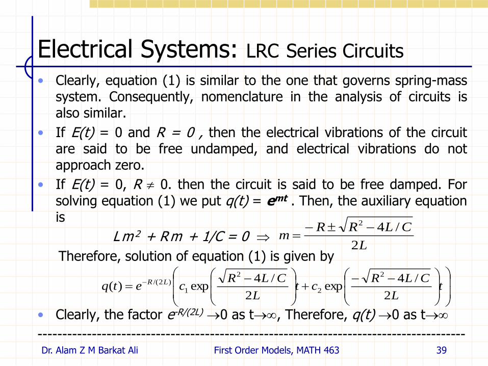
• Clearly, equation (1) is similar to the one that governs spring-masssystem. Consequently, nomenclature in the analysis of circuits isalso similar.
• If E(t) = 0 and R = 0 , then the electrical vibrations of the circuitare said to be free undamped, and electrical vibrations do notapproach zero.
• If E(t) = 0, R 0. then the circuit is said to be free damped. Forsolving equation (1) we put q(t) = emt . Then, the auxiliary equationis
Lm 2 + Rm + 1/C = 0
Therefore, solution of equation (1) is given by
• Clearly, the factor e-R/(2L) 0 as t, Therefore, q(t) 0 as t
---------------------------------------------------------------------------------------Dr. Alam Z M Barkat Ali First Order Models, MATH 463 39
L
CLRRm
2
/42
t
L
CLRct
L
CLRcetq LR
2
/4exp
2
/4exp)(
2
2
2
1
)2/(
Electrical Systems: LRC Series Circuits
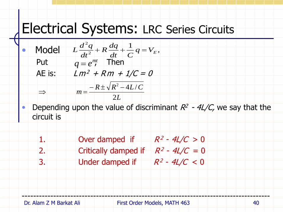
• Model
Put , Then
AE is: Lm 2 + Rm + 1/C = 0
• Depending upon the value of discriminant R2 - 4L/C, we say that thecircuit is
1. Over damped if R 2 - 4L/C > 0
2. Critically damped if R 2 - 4L/C = 0
3. Under damped if R 2 - 4L/C < 0
---------------------------------------------------------------------------------------Dr. Alam Z M Barkat Ali First Order Models, MATH 463 40
,1
2
2
EVqCdt
dqR
dt
qdL
mteq
L
CLRRm
2
/4
2

Example 6: Underdamed LRC Series Circuit
• A zero volt battery is connected to an LRC series circuit, in whichinductance is L = 0.25 henrys, resistance is R = 10 andcapacitance is C = 0.001 Farad. Initially 4 coulombs of charge ispresent on the capacitor and initial current in the circuit is 0.
Set up a mathematical model to find electric charge on the capacitorat any time t.
Solve the model analytically and find a formula for the elecyriccharge on the capacitor at time t.
Draw simulation block diagram, use it to simulate the model andanalyze simulation result.
---------------------------------------------------------------------------------------
Dr. Alam Z M Barkat Ali First Order Models, MATH 463 41
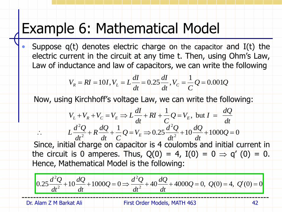
Example 6: Mathematical Model• Suppose q(t) denotes electric charge on the capacitor and I(t) the
electric current in the circuit at any time t. Then, using Ohm’s Law,Law of inductance and law of capacitors, we can write the following
Now, using Kirchhoff’s voltage Law, we can write the following:
Since, initial charge on capacitor is 4 coulombs and initial current inthe circuit is 0 amperes. Thus, Q(0) = 4, I(0) = 0 q’ (0) = 0.Hence, Mathematical Model is the following:
---------------------------------------------------------------------------------------Dr. Alam Z M Barkat Ali First Order Models, MATH 463 42
QQC
Vdt
dI
dt
dILVIRIV CLR 001.0
1 ,0.25 ,10
dt
dQIVQ
CRI
dt
dILVVVV EECRL but ,
1
010001025.0 1
2
2
2
2
Qdt
dQ
dt
QdVQ
Cdt
dQR
dt
QdL E
0)0( ,4)0( ,0400040010001025.02
2
2
2
QQQdt
dQ
dt
QdQ
dt
dQ
dt
Qd

Example 6: Analytical Solution
•
------------------------------------------------------------------------Dr. Alam Z M Barkat Ali First Order Models, MATH 463 43
0)0( ,4)0( ,010001025.02
2
QQQdt
dQ
dt
Qd

Example 6: Block diagram
•
------------------------------------------------------------------------Dr. Alam Z M Barkat Ali First Order Models, MATH 463 44
0)0( ,4)0( ,40004004000402
2
2
2
QQQdt
dQ
dt
QdQ
dt
dQ
dt
Qd

Example 6: Simulation Result/Scope
•
------------------------------------------------------------------------Dr. Alam Z M Barkat Ali First Order Models, MATH 463 45
We see that
electric charge
on capacitor
oscillates
initially with
decreasing
amplitude
and becomes
0 after about
0.2 seconds,
in agreement
with analytical
solution.
Notice the
similarity with
graph in
example 4.

Analogy Between electrical systems andmechanical Systems.
Dr. Alam Z M Barkat Ali First Order Models, MATH 463 46
•
------------------------------------------------------------------------

Second Order Models Mechanical / Electrical Systems
----------------------------------------------------------------
Dr. Alam Z M Barkat Ali First Order Models, MATH 463 47