mathematical modelling of the electrical wave in the heart from ion

Mathematical modelling of the electrical wave inthe heart from ion-channels to the body surface.Direct and inverse problems

Nejib ZemzemiCIMPA school 2016

Abstract This document presents a concise overview of various mathematical andnumerical problems raised by the simulation of electrocardiograms (ECGs). Amodel for the propagation of the electrical activation in the heart and in the torsois proposed. Some of its mathematical properties are analyzed. This model is notaimed at reproducing the complex phenomena taking place at the microscopic level.It has been devised to produce realistic healthy ECGs, and some pathological ones,with a reasonable level of complexity. It relies on various assumptions that are care-fully discussed through their impact on the ECGs. The coupling between the heartand the torso is a critical numerical issue which is addressed. In particular efficientcoupling strategies based on explicit algorithms are presented and analyzed. We alsostudy the coupling between the myocardium cells and the rapid conduction systemin the heart. Two applications related to the inverse problem in the electrocardiog-raphy are addressed. The first concerns the optimization of the conductivities insidethe torso cage. The second concerns the study of the conductivity values uncertain-ties on the constructed heart signals.

Nejib ZemzemiInria Bordeaux Sud-Ouest, Carmen team project

e-mail: [email protected]

1

[email protected]

Contents

Mathematical modelling of the electrical wave in the heart fromion-channels to the body surface. Direct and inverse problems . . . . . . . . . . 1CIMPA school 2016

1 Introduction . . . . . . . . . . . . . . . . . . . . . . . . . . . . . . . . . . . . . . . . . . . . . . . . . . . 7

Part I Éléments d’électrophysiologie et modélisation

2 Anatomie cardiaque et électrocardiogramme . . . . . . . . . . . . . . . . . . . . . . 111 Le cœur . . . . . . . . . . . . . . . . . . . . . . . . . . . . . . . . . . . . . . . . . . . . . . . . . 112 Fonctionnement du cœur . . . . . . . . . . . . . . . . . . . . . . . . . . . . . . . . . . . 12

2.1 Rôle du coeur . . . . . . . . . . . . . . . . . . . . . . . . . . . . . . . . . . . . . 122.2 Les battements cardiaques en électrophysiologie . . . . . . . 13

3 La circulation sanguine . . . . . . . . . . . . . . . . . . . . . . . . . . . . . . . . . . . . 133.1 Petite circulation . . . . . . . . . . . . . . . . . . . . . . . . . . . . . . . . . . 143.2 Grande circulation . . . . . . . . . . . . . . . . . . . . . . . . . . . . . . . . . 15

4 L’électrocardiogramme . . . . . . . . . . . . . . . . . . . . . . . . . . . . . . . . . . . . 164.1 Définition . . . . . . . . . . . . . . . . . . . . . . . . . . . . . . . . . . . . . . . . 164.2 Cadre historique . . . . . . . . . . . . . . . . . . . . . . . . . . . . . . . . . . 16

3 Modèles mathématiques . . . . . . . . . . . . . . . . . . . . . . . . . . . . . . . . . . . . . . . . 211 Modèle OD: échelle cellulaire . . . . . . . . . . . . . . . . . . . . . . . . . . . . . . . 21

1.1 Les canaux ioniques . . . . . . . . . . . . . . . . . . . . . . . . . . . . . . . 211.2 Les pompes . . . . . . . . . . . . . . . . . . . . . . . . . . . . . . . . . . . . . . 241.3 Les échangeurs . . . . . . . . . . . . . . . . . . . . . . . . . . . . . . . . . . . 241.4 Modélisation de la membrane cellulaire cardiaque . . . . . . 25

2 Le modèle 3D: échelle macroscopique . . . . . . . . . . . . . . . . . . . . . . . . 262.1 Le modèle bidomaine . . . . . . . . . . . . . . . . . . . . . . . . . . . . . . 27

3 Modèle du thorax . . . . . . . . . . . . . . . . . . . . . . . . . . . . . . . . . . . . . . . . . 304 Couplage avec le thorax . . . . . . . . . . . . . . . . . . . . . . . . . . . . . . . . . . . . 31

3

Part II Mathematical analysis: Existence and uniqueness of the bidomain-torso coupled problem

4 Existence and uniqueness of the bidomain-torso coupled problem . . . 371 Introduction . . . . . . . . . . . . . . . . . . . . . . . . . . . . . . . . . . . . . . . . . . . . . 372 Main result . . . . . . . . . . . . . . . . . . . . . . . . . . . . . . . . . . . . . . . . . . . . . . . 413 Existence of weak solution of the bidomain-torso problem . . . . . . . 44

3.1 A regularized problem in finite dimension . . . . . . . . . . . . . 443.2 Local existence of the discretized solution . . . . . . . . . . . . . 453.3 Energy estimates . . . . . . . . . . . . . . . . . . . . . . . . . . . . . . . . . . 483.4 Weak solution of the bidomain-torso problem . . . . . . . . . . 54

4 Uniqueness of the weak solution . . . . . . . . . . . . . . . . . . . . . . . . . . . . . 56

Part III Numerical analysis and Simulation of ECGs

5 Mathematical modeling of Electrocardiograms: A numerical study . . 611 Introduction . . . . . . . . . . . . . . . . . . . . . . . . . . . . . . . . . . . . . . . . . . . . . . 612 Modeling . . . . . . . . . . . . . . . . . . . . . . . . . . . . . . . . . . . . . . . . . . . . . . . . 63

2.1 Heart tissue . . . . . . . . . . . . . . . . . . . . . . . . . . . . . . . . . . . . . . 632.2 Coupling with torso . . . . . . . . . . . . . . . . . . . . . . . . . . . . . . . . 65

3 Numerical methods . . . . . . . . . . . . . . . . . . . . . . . . . . . . . . . . . . . . . . . . 663.1 Space and time discretization . . . . . . . . . . . . . . . . . . . . . . . . 663.2 Partitioned heart-torso coupling . . . . . . . . . . . . . . . . . . . . . . 68

4 Numerical results . . . . . . . . . . . . . . . . . . . . . . . . . . . . . . . . . . . . . . . . . 694.1 Reference simulation . . . . . . . . . . . . . . . . . . . . . . . . . . . . . . 704.2 Bundle brunch blocks simulations . . . . . . . . . . . . . . . . . . . . 774.3 Simulations of arrhythmia . . . . . . . . . . . . . . . . . . . . . . . . . . 81

5 Impact of some modeling assumptions . . . . . . . . . . . . . . . . . . . . . . . . 835.1 Heart-torso uncoupling . . . . . . . . . . . . . . . . . . . . . . . . . . . . . 845.2 Study of the monodomain model . . . . . . . . . . . . . . . . . . . . . 885.3 Isotropy . . . . . . . . . . . . . . . . . . . . . . . . . . . . . . . . . . . . . . . . . 925.4 Cell homogeneity . . . . . . . . . . . . . . . . . . . . . . . . . . . . . . . . . 945.5 Capacitive and resistive effect of the pericardium . . . . . . . 95

6 Numerical investigations with weak heart-torso coupling . . . . . . . . 986.1 Time and space convergence . . . . . . . . . . . . . . . . . . . . . . . . 986.2 Sensitivity to model parameters . . . . . . . . . . . . . . . . . . . . . . 100

7 Conclusion . . . . . . . . . . . . . . . . . . . . . . . . . . . . . . . . . . . . . . . . . . . . . . . 103

6 Decoupled time-marching schemes in computational cardiacelectrophysiology and ECG numerical simulation . . . . . . . . . . . . . . . . . . 1051 Introduction . . . . . . . . . . . . . . . . . . . . . . . . . . . . . . . . . . . . . . . . . . . . . . 1052 Mathematical models . . . . . . . . . . . . . . . . . . . . . . . . . . . . . . . . . . . . . . 107

2.1 Isolated heart . . . . . . . . . . . . . . . . . . . . . . . . . . . . . . . . . . . . . 1072.2 Coupling with torso: ECG modeling . . . . . . . . . . . . . . . . . . 109

3 Decoupled time-marching for the bidomain equation . . . . . . . . . . . . 111

3.1 Preliminaries . . . . . . . . . . . . . . . . . . . . . . . . . . . . . . . . . . . . . 1113.2 Time semi-discrete formulations: decoupled

time-marching schemes . . . . . . . . . . . . . . . . . . . . . . . . . . . . 1123.3 Stability analysis . . . . . . . . . . . . . . . . . . . . . . . . . . . . . . . . . . 113

4 Decoupled time-marching for ECG numerical simulation . . . . . . . . 1174.1 Preliminaries . . . . . . . . . . . . . . . . . . . . . . . . . . . . . . . . . . . . . 1174.2 Fully discrete formulation: decoupled time-marching

schemes . . . . . . . . . . . . . . . . . . . . . . . . . . . . . . . . . . . . . . . . . 1194.3 Stability analysis . . . . . . . . . . . . . . . . . . . . . . . . . . . . . . . . . . 120

5 Numerical results . . . . . . . . . . . . . . . . . . . . . . . . . . . . . . . . . . . . . . . . . 1235.1 Simulation data . . . . . . . . . . . . . . . . . . . . . . . . . . . . . . . . . . . 1235.2 Isolated heart . . . . . . . . . . . . . . . . . . . . . . . . . . . . . . . . . . . . . 1255.3 12-lead ECG . . . . . . . . . . . . . . . . . . . . . . . . . . . . . . . . . . . . . 126

6 Conclusion . . . . . . . . . . . . . . . . . . . . . . . . . . . . . . . . . . . . . . . . . . . . . . . 127

7 Stability analysis of time-splitting schemes for the specializedconduction system/myocardium coupled problem in cardiacelectrophysiology . . . . . . . . . . . . . . . . . . . . . . . . . . . . . . . . . . . . . . . . . . . . . . . 1411 Introduction . . . . . . . . . . . . . . . . . . . . . . . . . . . . . . . . . . . . . . . . . . . . . . 1412 Modelling . . . . . . . . . . . . . . . . . . . . . . . . . . . . . . . . . . . . . . . . . . . . . . . 144

2.1 Mathematical models . . . . . . . . . . . . . . . . . . . . . . . . . . . . . . 1443 Stability analysis of the semi-discretized problem . . . . . . . . . . . . . . 146

3.1 Space discretization . . . . . . . . . . . . . . . . . . . . . . . . . . . . . . . . 1464 Stability of the time-splitting schemes . . . . . . . . . . . . . . . . . . . . . . . . 150

4.1 Time discretization . . . . . . . . . . . . . . . . . . . . . . . . . . . . . . . . 1504.2 Stability of the time-splitting schemes . . . . . . . . . . . . . . . . 152

5 Numerical results . . . . . . . . . . . . . . . . . . . . . . . . . . . . . . . . . . . . . . . . . 1575.1 1D/2D coupling case: Convergence analysis . . . . . . . . . . . 1585.2 Accuracy of the numerical schemes . . . . . . . . . . . . . . . . . . 1595.3 1D-3D numerical results . . . . . . . . . . . . . . . . . . . . . . . . . . . . 161

6 Conclusion . . . . . . . . . . . . . . . . . . . . . . . . . . . . . . . . . . . . . . . . . . . . . . . 167

Part IV Applications

8 Inverse problems in Electrocardiography . . . . . . . . . . . . . . . . . . . . . . . . . 1731 Introduction . . . . . . . . . . . . . . . . . . . . . . . . . . . . . . . . . . . . . . . . . . . . . . 1732 Sensitivity . . . . . . . . . . . . . . . . . . . . . . . . . . . . . . . . . . . . . . . . . . . . . . . 1743 Estimation of the torso conductivity parameters . . . . . . . . . . . . . . . . 174

3.1 Numerical experiment . . . . . . . . . . . . . . . . . . . . . . . . . . . . . . 1753.2 Parameter estimation using synthetic data . . . . . . . . . . . . . 178

4 Ionic parameter estimation . . . . . . . . . . . . . . . . . . . . . . . . . . . . . . . . . . 1795 Conclusion . . . . . . . . . . . . . . . . . . . . . . . . . . . . . . . . . . . . . . . . . . . . . . . 179

9 Stochastic Finite Element Method for torso conductivityuncertainties quantification in electrocardiography inverse problem . 1831 Introduction . . . . . . . . . . . . . . . . . . . . . . . . . . . . . . . . . . . . . . . . . . . . . . 1832 Stochastic forward problem of electrocardiography . . . . . . . . . . . . 185

2.1 Function spaces and notation . . . . . . . . . . . . . . . . . . . . . . . . 1852.2 Stochastic formulation of the forward problem . . . . . . . . . 1862.3 Descretization of the stochastic forward problem . . . . . . . 187

3 Stochastic inverse problem of electrocardiography . . . . . . . . . . . . . 1893.1 Computation of the gradients . . . . . . . . . . . . . . . . . . . . . . . . 1893.2 The conjugate gradient algorithm. . . . . . . . . . . . . . . . . . . . . 192

4 Numerical results: Analytical case . . . . . . . . . . . . . . . . . . . . . . . . . . . 1934.1 Sensitivity of the forward problem to the conductivity

uncertainties . . . . . . . . . . . . . . . . . . . . . . . . . . . . . . . . . . . . . . 1944.2 Sensitivity of the inverse solution to the conductivity

uncertainties . . . . . . . . . . . . . . . . . . . . . . . . . . . . . . . . . . . . . . 1954.3 Sensitivity of the inverse solution to the distance

between the complete and incomplete boundaries . . . . . . . 1975 Electrocardiography imaging inverse problem . . . . . . . . . . . . . . . . . 198

5.1 Anatomical model . . . . . . . . . . . . . . . . . . . . . . . . . . . . . . . . . 1985.2 Numerical results . . . . . . . . . . . . . . . . . . . . . . . . . . . . . . . . . . 200

6 Discussion . . . . . . . . . . . . . . . . . . . . . . . . . . . . . . . . . . . . . . . . . . . . . . . 2037 Conclusions . . . . . . . . . . . . . . . . . . . . . . . . . . . . . . . . . . . . . . . . . . . . . . 203References . . . . . . . . . . . . . . . . . . . . . . . . . . . . . . . . . . . . . . . . . . . . . . . . . . . . . 205

Chapter 1Introduction

Le cœur est l’un des organes vitaux du corps humain, son rôle est de faire circulerle sang dans tous les tissus de l’organisme. Malgré son petit volume (entre 50 et60 cm3), il est chargé de pomper 8000 litres de sang par jour. Pour faire circulercette grande quantité, il doit battre sans s’arrêter plus de 100 000 fois par jour.Son arrêt peut être fatal. Comme tous les organes du corps humain, il peut être af-fecté de nombreuses pathologies. Ces dernières peuvent être sans danger, commecertaines tachycardies par exemple, ou bien s’avérer très sérieuses, comme les fib-rillations et les blocs de branches. L’évolution des technologies a permis au médecind’observer l’état du cœur à travers des outils d’imagerie médicale. Ceux-ci peuventêtre basés sur des ultrasons (echocardiographie), de la résonance magnétique (IRM)ou des rayons X. Ces technologies sont incontournables pour dresser un diagnosticdu cœur, mais leur utilisation demeure complexe et coûteuse. En 2006, il y avaitseulement 370 IRM installées dans toute la France, le coût d’un appareil est de 1,5M d’euros et le coût d’un examen est en moyenne de 315 euros (d’après l’institutCurie).

L’électrocardiogramme (ECG) est un outil clinique performant, non invasif, peucoûteux et facile à mettre en œuvre. Il est l’examen le plus couramment utilisé enélectrocardiologie. Les travaux présentés dans ce document concernent la modéli-sation et la simulation numérique de l’activité électrique du cœur, en particulierla modélisation et la simulation numérique des électrocardiogrammes. Nous avonschoisi de nous concentrer sur l’ECG pour deux raisons. La première est la per-formance de cet outil et son importance auprès des médecins (il s’agit du premierélément du diagnostic du cœur). La deuxième raison est que cet outil nous permetde dialoguer avec les cardiologues, ce qui nous permet d’avoir un retour critique surnos résultats de simulation. Il est en effet plus familier pour un médecin d’évaluerun ECG que la propagation de l’onde électrique dans le myocarde.

La modélisation du vivant est devenue un défi scientifique très important. Ellepourrait aider à mieux comprendre les phénomènes physiologiques et apporter dessolutions à des problèmes cliniques. En effet, les expériences in vivo ne sont par-fois pas réalisables à cause de contraintes pratiques ou morales. Avoir un outilnumérique prédictif capable de reproduire le phénomène physiologique fournirait

7

en quelque sorte un “cobaye virtuel”. Ce cobaye pourrait servir à réaliser des ex-périences dans le but de résoudre des problèmes biomédicaux ou industriels. L’étudede ces phénomènes permet aussi de faire évoluer les sciences physique mathéma-tiques en proposant des nouvelles problématiques et peut en même temps inciter lechercheur à trouver des nouvelles méthodes pour résoudre les problèmes soulevés.

Part IÉléments d’électrophysiologie et

modélisation

Chapter 2Anatomie cardiaque et électrocardiogramme

1 Le cœur

Le cœur est un muscle creux formé principalement de fibres enroulés (voir Figure 1),une pompe composée de tissu musculaire, qui recueille sans cesse le sang et lepropulse dans les artères. C’est le seul muscle qui peut se contracter régulièrementsans fatigue, tandis que les autres muscles ont besoin d’une période de repos. Il setrouve au milieu de la cage thoracique délimitée par les deux poumons, le sternumet la colonne vertébrale, il se situe un peu à gauche du centre du thorax au-dessusdu diaphragme.

Fig. 1 Orientation des fibres (d’après bembook [MP95]).

Alors que la masse du cœur (350 g) n’excède pas 0,5 % de la masse du corps,il prélève 10% de la consommation totale d’oxygène; il est alimenté en oxygèneet nutriments par les vaisseaux coronaires, qui forment autour de lui une sorte decouronne. Le cœur est composé de quatre chambres (deux oreillettes et deux ven-

11

Fig. 2 Anatomie du coeur (Source: Encyclopédie Larousse)

tricules), équipées de valves qui empêchent les reflux sanguins. Il pompe le sanggrâce à une série de systoles (contractions) et diastoles (relâchements) des oreil-lettes et ventricules. La circulation sanguine étant à sens unique, les valves ont pourbut d’empêcher le sang de revenir en arrière: la valve tricuspide sépare l’oreillettedroite du ventricule droit, la valve mitrale sépare l’oreillette gauche du ventriculegauche. Les artères sont séparés des ventricules par les valves sigmoides: le ven-tricule gauche est séparé de l’artère pulmonaire par les valves pulmonaires et leventricule gauche est séparé de l’aorte par les valves aortiques. Par contre il n’existepas de séparation entre les veines et les oreillettes.

2 Fonctionnement du cœur

2.1 Rôle du coeur

Le cœur se contracte très régulièrement et la continuité de ses battements est essen-tielle à la vie: un arrêt de la pulsation cardiaque est l’un des signes les plus évidentsd’un décès. Ces pulsations, qui permettent à du sang frais, oxygéné, d’irriguer lesorganes, ne peuvent s’arrêter, même durant une période très courte: certains or-ganes peuvent survivre à une brève interruption des pulsations cardiaques, d’autresnon. C’est le cas du cerveau, qui est extrêmement sensible à toute anomalie circu-latoire: 10 minutes d’interruption de l’irrigation sanguine du cerveau suffisent pour

endommager l’organe de façon irréversible et la mort s’ensuit. Un cœur au reposse contracte normalement environ 70 fois par minute, période au cours de laque-lle il chasse 5 litres de sang (le volume sanguin total d’un Homme). La contrac-tion du cœur se fait d’une manière intrinsèque, c’est-à-dire qu’aucune stimulationd’origine nerveuse n’intervient. Une cellule musculaire cardiaque isolée continueà battre spontanément et rythmiquement. Ensemble, les cellules musculaires con-stituent la paroi du cœur ou myocarde. Bien que le cœur génère son propre rythmecontractile (le pouls), celui-ci est régulé par le système nerveux et deux hormones: L’adrénaline et la noradrénaline, hormones sécrétées par les glandes surrénalesen cas de peur ou de colère, augmentent le rythme des contractions cardiaques; lanoradrénaline est aussi libérée par les fibres nerveuses sympathiques arrivant aumyocarde, l’acétylcholine, substance libérée par les nerfs parasympathiques, agit aucontraire sur le cœur en ralentissant le pouls. Le rythme cardiaque varie de 70 batte-ments par minutes (au repos) à 180, voire 210 battements par minute lors d’effortsintenses.

2.2 Les battements cardiaques en électrophysiologie

Les battements cardiaques sont sous le contrôle d’un pacemaker naturel, sorte degroupement de cellules du myocarde qui constituent le nœud sinusal ou nœud sino-auriculaire (SA), situé en haut de l’oreillette droite. Le nœud SA donne naissanceà une onde d’excitation tous les 0.8 seconde. Cette onde parcourt, pendant 0.1 sec-onde, le tissu musculaire des deux oreillettes, qui se contractent d’abord lorsque lesventricules sont au repos. Cette periode correspond dans l’ECG à la duré de l’ondeP. Puis l’onde gagne le second nœud, le nœud auriculo-ventriculaire (ou nœud AV)situé plus bas entre les deux oreillettes, lequel transmet l’onde d’excitation auxparois des deux ventricules via le faisceau auriculo-ventriculaire (ou le faisceau deHis) puis les fibres de Purkinje. Ces dernières, en contact direct avec le myocarde,lui transmettent le courant ce qui entraine la dépolarisation et la contraction des cel-lules. Cette periode correspond au complexe QRS de l’ECG. Lorsque les ventriculesse contractent, les oreillettes sont au repos. Le bruit du coeur provient de la brusquefermeture des valves à chaque contraction.

3 La circulation sanguine

L’Homme possède un système circulatoire clos: le sang part du cœur en emprun-tant les artères puis les artérioles, il traverse le réseau capillaire soit au niveau despoumons (petite circulation ou circulation pulmonaire), soit au niveau des autres or-ganes (grande circulation ou circulation systémique), puis il retourne au coeur parles veinules puis les veines. Les artères sont des vaisseaux sanguins qui vont du cœurvers les organes, les veines ramenant inversement le sang des organes vers le cœur.

1.2 - Fonctionnement du cœur 19

Figure 5: Etapes de la progression de la contraction cardiaque et composantes corre-spondantes d’un électrocardiogramme (d’après Bembook [MP95]).

du ventricule gauche et les valves sigmoides sont situées entre les ventricules et les artères(les valves aortique ou pulmonaire par exemple); il n’y a pas de valves entre les veineset les oreillettes.


L’Homme, comme tous les vertébrés, possède un système circulatoire clos, contraire-ment à son système vasculaire lymphatique: le sang part du cœur en empruntant lesartères puis les artérioles, il traverse le réseau capillaire soit au niveau des poumons

18 Anatomie du cœur
























L’Homme, comme tous les vertébrés, possède un système circulatoire clos, contraire-ment à son système vasculaire lymphatique: le sang part du cœur en empruntant lesartères puis les artérioles, il traverse le réseau capillaire soit au niveau des poumons(petite circulation ou circulation pulmonaire), soit au niveau des autres organes (grandecirculation ou circulation systémique), puis il retourne au coeur par les veinules puis lesveines. Les artères sont donc des vaisseaux sanguins qui vont du cœur vers les organes,les veines ramenant inversement le sang des organes vers le cœur. Dans la grande circula-tion, les artères, partant du ventricule gauche, transportent donc du sang oxygéné rougeet les veines, revenant à l’oreillette droite, transportent du sang carbonaté bleu. Parcontre, dans la petite circulation, les artères pulmonaires, partant du ventricule droit,transportent du sang carbonaté vers les poumons, et les veines pulmonaires ramènent àl’oreillette gauche du sang oxygéné.

Dans la grande circulation, les organes sont généralement vascularisés par une artèreprovenant d’une ramification de l’aorte qui part du ventricule gauche, et dont le quali-ficatif rappelle le nom de l’organe (artère rénale pour "artère du rein", artère humérale

18 Anatomie du cœur1.2 - Fonctionnement du cœur 19













































Dans la grande circulation, les organes sont généralement vascularisés par une artèreprovenant d’une ramification de l’aorte qui part du ventricule gauche, et dont le quali-ficatif rappelle le nom de l’organe (artère rénale pour "artère du rein", artère huméralepour "artère de l’humérus", etc.). De façon comparable, les veines semblablement nom-mées se jettent dans les veines caves inférieure ou supérieure qui ramènent le sang vers

18 Anatomie du cœur1.2 - Fonctionnement du cœur 19













































Dans la grande circulation, les organes sont généralement vascularisés par une artèreprovenant d’une ramification de l’aorte qui part du ventricule gauche, et dont le quali-ficatif rappelle le nom de l’organe (artère rénale pour "artère du rein", artère huméralepour "artère de l’humérus", etc.). De façon comparable, les veines semblablement nom-mées se jettent dans les veines caves inférieure ou supérieure qui ramènent le sang vers

Fig. 3 Etapes de la progression de la contraction cardiaque et composantes correspondantes d’unélectrocardiogramme (d’après Bembook [MP95]).

Dans la grande circulation, les artères, partant du ventricule gauche, transportentdu sang oxygéné (rouge) et les veines, revenant à l’oreillette droite, transportent dusang chargé en dioxyde de carbone (bleu), voir Figure 4. Par contre, dans la petitecirculation, les artères pulmonaires, partant du ventricule droit, transportent du sangchargé en dioxyde de carbone vers les poumons, et les veines pulmonaires ramènentà l’oreillette gauche du sang oxygéné.

3.1 Petite circulation

Le myocarde étant dans sa phase de décontraction, la pression sanguine est plusélevée dans les artères que dans le cœur en diastole, de sorte que les valves sig-moides (valves pulmonaire et aortique) sont fermées, entre-temps les oreillettes seremplissent de sang provenant des veines. Le sang qui vient de l’oreillette droitepasse, à travers la valve triscupide, dans le ventricule droit. Les contractions du ven-tricule droit envoient le sang dans l’artère pulmonaire qui pénètre dans les poumonset s’y ramifie en capillaires pulmonaires. Ces derniers se rassemblent en veines pul-monaires qui aboutissent à l’oreillette gauche. Le cycle est ainsi bouclé.

3.2 Grande circulation!"#$%&'()*) ) +(),-.')(&)/01/(,&'2,#'3%24'#$"%())

) *5

)

!"#$%&'(')'*&'+,+-./&'0%-1%"&*'&-'*&'+,+-./&'2&"3&$4'+53-'6&$4'%1+&0$4'75/8*1/&3-0"%&+'6&'20"++&0$4'

+03#$"3+9' :03+' *0' #%036&' 7"%7$*0-"53;' *&' 8%&/"&%' 0++$%&' *&' -%03+85%-' 6$' +03#' 54,#131' 2&%+' *&+'

5%#03&+;'*&'+&7536'*&'%&-5$%'6$'+03#'80$2%&'&3'54,#.3&9'<=1*1/&3-'7&3-%0*'&+-'*&'7>$%'?$"'8%57$%&'

*0'8%&++"53'317&++0"%&'@'7&--&'7"%7$*0-"53'AB5$%7&')'C--8)DDEEEF%57?9"3%"09G%DH0%79IC"%"&-DJ*5+%DK"5'

DL88M"%7$*DM"%7$*9C-/*N9'

))))

)

!"#$! $%&$'()*$$

)

+()),-.')(6&))/01/17(8&),(8&'#/)3.)696&:7(),#'3%2;#6,./#%'(<)=2.6)31,'%;286)3#86)/#)6.%&()3.)

,"#$%&'()/0#8#&27%()(&)/()>28,&%288(7(8&)1/(,&'%?.()30.8),-.')6#%8<)

)

!"#"+$! ,-./012&$

)

+(),-.') )$'2$./6() /()6#84)4'@,()#.A),28&'#,&%286)3()628) &%66.)7.6,./#%'()#$$(/1)792,#'3(<)

B8()1$#%66() ,/2%628) /()3%;%6() (8)3(.A)72%&%16) C,-.')4#.,"(D,-.')3'2%&EF) (&) ,"#,.8()30(//(6)

,27$2'&()3(.A),#;%&16)G) /02'(%//(&&()(&)/();(8&'%,./(<)H),"#?.()I#&&(7(8&F)/()792,#'3()6.%&)/#)

7J7()61?.(8,()3()72.;(7(8&)G)/()6#84)$#.;'()(8)2A94:8()#''%;()#.),-.')$#')/#);(%8(),#;(<)

K/)9)(8&'()$#')/02'(%//(&&()3'2%&(F)(&)(8)(6&),"#661)$#')6#),28&'#,&%28)#$$(/1()!"!#$%&'()*+,)%(+*&)

?.%) /()31$/#,()3#86) /();(8&'%,./()3'2%&<)+#)696&2/()-&.#*+,)%(+*&) C,28&'#,&%28)3(6);(8&'%,./(6E)

$'2$./6() L) 628) &2.') /() 6#84) 3.) ;(8&'%,./() 3'2%&) ;('6) /(6) $2.7286) 2M) %/) ;#) 6() ,"#'4(') (8)

Fig. 4 Représentation schématique de la petite et la grande circulations sanguines: Les flchesrouges designe le sens de circulation du sang oxygéné et les flèches bleus designe le sens de cir-culation du sang riche en CO2. Source: http://www-rocq.inria.fr/Marc.Thiriet/Glosr/Bio/AppCircul/Circul.html

Quand la stimulation contractile atteint le myocarde, ceci provoque la contractiondes ventricules: cette systole ferme les valves tricuspide et mitrale. La pression dansles ventricules devient tellement élevée que les valves sigmoides s’ouvrent: le sangafflue dans les artères. En particulier, le sang sortant du ventricule gauche passe àtravers la valve aortique vers l’aorte. Les organes sont généralement vascularisés parune artère provenant d’une ramification de l’aorte. Le sang qui pénètre dans le foieprovient de deux sources: l’artère hépatique apporte du sang oxygéné par la circula-tion systémique, et la veine porte hépatique apporte du sang carbonaté mais riche ennutriments, provenant des organes digestifs. Le système porte hépatique rassemblele sang veineux venant de l’estomac (via la veine gastrique), du pancréas (via laveine pancréatique), de l’intestin (via les veines mésentériques) et aussi de la rate(via la veine splénique). Le foie contrôle les nutriments ainsi apportés, emmagasinele glucose (sous forme de glycogène) et filtre certaines substances nocives commel’alcool ou la caféine ou la théobromine du cacao. Enfin, le sang quitte le foie par

http://www-rocq.inria.fr/Marc.Thiriet/Glosr/Bio/AppCircul/Circul.html

http://www-rocq.inria.fr/Marc.Thiriet/Glosr/Bio/AppCircul/Circul.html

la veine sus-hépatique, qui se jette dans la veine cave inférieure. De façon compara-ble, d’autres veines provenant de membres supérieurs, de la tête et du cou se jettentsemblablement, dans la veine cave supérieure. Les deux veines caves supérieure etinférieure ramènent le sang vers l’oreillette droite.

4 L’électrocardiogramme

4.1 Définition

L’électrocardiogramme est une représentation graphique de l’activité électrique ducoeur. L’électrocardiographe qui est l’appareil permettant de faire un ECG, mesurela différence de potentiel entre différentes positions de la surface du corps. Cequi permet d’avoir une description non invasive de l’état du cœur. Le médecinpeut visualiser ces différences de potentiel sur un écran appelé électrocardioscope.L’électrocardiogramme peut aussi être tracé sur un papier millimétré. Ce papier ap-pelé “papier pour ECG” est tracé en petits et grands carrés de tailles respectives1mm et 5mm (voir Figure. 5). Horizontalement, un petit carreau (respectivement,un grand carreau) représente 40 ms (respectivement, 200 ms) et verticalement 1 mv(respectivement, 5 mv). L’électrocardiogramme affiché sur la Figure. 5 représentela première dérivation de l’ECG d’un cœur en situation normale. Les différentesfluctuations qu’on regarde sur cet ECG s’appellent, dans l’ordre de gauche à droite,les ondes P, Q, R, S, T et U.

• L’onde P, représente la dépolarisation auriculaire,• le complexe QRS, représente la dépolarisation des ventricules,• le segment QT, représente le plateau des potentiels d’action ventriculaire,• L’onde T, correspond à la repolarisation des ventricules,• L’onde U, généralement absente, est provoquée par une repolarisation prolongée

des cellules M ou par un facteur mécanique correspondant à la relaxation dumyocarde.

4.2 Cadre historique

L’ECG est un outil médical récent. Son histoire a commencé à la fin du XVIII èmesiècle. Au cour d’un siècle et demi les chercheurs ont trouvé la forme “idéale” del’ECG. L’ECG qu’utilisent actuellement les cliniciens date du début du XX èmesiècle.

Historiquement, la première personne qui a remarqué que le muscle bouge quandil est excité est le médecin et physicien italien Luigi Galvani. Il découvre en 1771que les muscles d’une grenouille morte bougent lorsqu’elles sont mises en contactavec des métaux telsque le cuivre et le zinc (voir Figure. 6). Mais jusqu’à cette date,

Fig. 5 L’ECG d’un cycle cardiaque normale.

personne ne connaît l’origine de l’onde électrique qui traverse le corps d’un animal.

Ce n’est qu’après l’invention d’un outil de mesure du signal électrique, “le Gal-vanomètre1”, que les physiciens et les médecins commencent à relier les battementscardiaques à un signal électrique. En effet, le physicien italien Carlo Matteucci[Mat42], montre en 1842, pour la première fois, que chaque contraction du coeur estaccompagnée par un courant électrique. Un an après, le physiologiste allemand EmilDubois Reymond confirme les travaux de Matteucci et décrit un potentiel d’actionaccompagnant chaque contraction musculaire. Ce potentiel d’action a été enregistrépour la première fois en 1856 par les chercheurs allemand Rudolph von Koellikeret Heinrich Muller. Après l’invention de l’électromètre capillaire2 par le physicienfrançais Gabriel Lippmann, en 1872, cet appareil a été utilisé par le physiologistefrançais Étienne-Jules Marey [Mar76] en 1876 pour enregistrer l’activité électriquedu coeur d’une grenouille. Deux ans plus tard, les physiologistes britanniques JohnBurden Sanderson et Frederick Page [SP76] enregistrent le courant électrique car-

1 Appareil de mesure du signal électrique inventé par Johan Salomo et Christoph Schweigger en1821.2 C’est un tube de verre à colonne de mercure et d’acide sulfurique.

Fig. 6 Représentation de l’expérience de Galvani, qui lui a permis de découvrir l’électricité ani-male (gauche). Photo de Luigi Galvani (droite). Source: Wikipedia.

diaque avec l’électromètre capillaire et montrent qu’il est composé de deux phases(dépolarisation et repolarisation). Ces deux chercheurs publient en 1884 des enreg-istrements électriques faits sur le cœur d’une grenouille [SP84]. Trois ans après, lepremier électrocardiogramme humain a été enregistré par le physiologiste britan-nique Augustus D. Waller de St Mary’s Medical School, à Londres [Wal87]. Il estenregistré sur Thomas Goswell, un technicien du laboratoire. En 1889, le physiol-ogiste allemand Willem Einthoven (voir Figure. 7)3 démontre sa technique au Pre-mier Congrès International de Physiologie. En 1890, G.J. Burch d’Oxford imagineune correction arithmétique pour les observations de fluctuation de l’électromètre.Celui-ci permet de voir le vrai tracé de l’électrocardiogramme [Bur90].

Cinq ans plus tard, Einthoven, utilisant un électromètre amélioré ainsi qu’uneformule de correction développée indépendamment par Burch, met en évidence cinqdéflexions qu’il appelle P, Q, R, S and T [Ein95].

En 1901, Einthoven modifie cet enregistreur pour produire des électrocardio-grammes. Son appareil pèse 300 kg (voir Figure. 7) [Ein01]. L’année qui suit,Einthoven publie le premier électrocardiogramme enregistré avec cet appareil. Ilpublie, en 1906, la première classification des électrocardiogrammes normaux etanormaux: Hypertrophies ventriculaires gauches et droites, hypertrophies auricu-laires gauches et droites, ondes U, éléments sur le QRS, contractions ventricu-laires prématurées, bigéminisme ventriculaire, flutter auriculaire et bloc auriculo-ventriculaire complet [Ein06]. Six ans plus tard, il décrit un triangle équilatéralformé par les dérivations standards D1, D2, D3, appelé plus tard “triangle d’Einthoven”.C’est aussi la première fois qu’il utilise dans un article l’abréviation anglo-saxonnede l’électrocardiogramme EKG (ECG). En 1920, Hubert Mann du laboratoire decardiologie de l’hôpital du Mont Sinaï de New York, décrit la dérivation d’un

3 Source: wikipedia.

Fig. 7 Photo de l’électrographe d’Einthoven montrant la technique qu’il a utilisé: Les deux mainset le pied gauche sont plongés dans des jarres contenant de l’eau salée. Les trois jarres sont reliéesà l’appareil avec des fils électriques.

“monocardiogramme” plus tard appelé “vectocardiogramme” [Man20]. En 1924,Willem Einthoven obtient le prix Nobel pour l’invention de l’électrocardiographe.

L’American Heart Association et The Cardiac Society de Grande Bretagnedéfinissent, en 1938, les positions standards des dérivations précordiales V1, V2,. . . ,V6[RPW+38]. Enfin, en 1942, Emanuel Goldberger ajoute aux dérivations frontalesd’Einthoven les dérivations aVR, aVL, aVF. Ceci lui permet, avec les 6 dérivationsprécordiales V1,V2,. . . ,V6, de réaliser le premier électrocardiogramme sur 12 déri-vations, qui est encore utilisé aujourd’hui.

Chapter 3Modèles mathématiques

On peut distinguer deux échelles de modélisation en électrophysiologie cardiaque.On trouve d’une part des modèles s’intéressant à l’échelle microscopique, dont lebut est de produire une description fine de ce qui est à l’origine de l’onde électriquedans les cellules. On trouve d’autre part des modèles à l’échelle de l’organe, dontle but est de décrire la propagation de l’onde électrique dans le cœur et le reste ducorps. Dans ce qui suit, nous proposons de présenter les éléments principaux de cesdeux catégories. Nous avons choisi de nous limiter aux approches basées sur deséquations différentielles et aux dérivées partielles (nous ne présenterons donc pasde modèles basés sur des automates cellulaires).

1 Modèle OD: échelle cellulaire

Les cellules (en particulier les cellules cardiaques) sont entourées par une membranelimitant l’unité cellulaire, cette membrane est percée par des protéines dont le rôleest d’assurer le flux des différentes substances intra et extra-cellulaires à travers lamembrane (voir figure 8).

Ces protéines peuvent avoir un comportement passif ou actif selon l’état de la cel-lule, leur activité permet le passage de certaines substances chimiques à l’intérieurou à l’extérieur de la cellule, ce qui provoque la dépolarisation ou la répolarisationcellulaire. On peut classifier le processus du transport ionique en trois modes detransfert: les canaux ioniques, les pompes et les échangeurs.

1.1 Les canaux ioniques

Un canal ionique (Figure 9, gauche) laisse passer dans un sens donné une espèceconformément à son gradient électrochimique. Son comportement est simplementmodélisé par une résistance. Un canal ionique est cependant actif dans la mesure

21

Fig. 8 Représentation schématique de la membrane cellulaire. Source: www.bio-energetik.ca/images/cell_membrane.jpg

où sa conductivité est variable selon les conditions extérieures: en particulier il peutêtre fermé.

La dépolarisation de la cellule est généralement causée par l’ouverture d’un canalionique. Ce canal est celui du sodium Na+. Son ouverture se fait dans le sens de songradient électrochimique, par conséquent, il ne nécessite aucun apport d’énergie dela cellule. Ce genre de transport ionique est appelé transport passif. L’ouverture d’uncanal de sodium provoque la création d’un courant ionique iNa de l’ordre du pico-ampère (pA). Ce courant est proportionnel au gradient électrochimique du sodium(Vm−ENa) et à une variable qui représente l’ouverture et la fermeture de ce canalGNa. Le potentiel transmembranaire Vm est la différence entre le potentiel intra etextra-cellulaire. Le potentiel électrochimique ENa est donné par la loi de Nernst

ENa =RTF

ln[Na]e[Na]i

, (1)

où [Na]e (respectivement [Na]i) est la concentration extra-cellulaire (respectivementintra-cellulaire) de l’ion sodium Na+. Les constantes R, T et F indiquent respective-ment, la constante de gaz parfait, la temperature et la constante de Faraday.

Le courant iNa d’ions Na+ à travers ce canal, décrit par Hodgkin et Huxley (voir[HH52]) est donné par

iNa = GNa(Vm−ENa). (2)

Ce canal ionique n’est pas toujours ouvert. Sa fermeture et son ouverture suivent laloi de conductivité des portes des canaux ioniques GNa qui peut être réprésentée de

www.bio-energetik.ca/ images/cell_membrane.jpg

www.bio-energetik.ca/ images/cell_membrane.jpg

la manière suivante:GNa = GNaH, (3)

où GNa est la conductivité maximale du canal ionique représentant son ouverturemaximale. La fonction H est comprise entre 0 et 1, elle est donnée par,

H = H(Vm, [Nai], [Nae]...). (4)

Fig. 9 Représentation schématique des canaux ioniques Na+, K+ et Ca2+ (gauche) et dela pompe Na+/K+ (droite). Source: http://www.apteronote.com/revue/neurone/article_79.shtml

Le canal ionique Na+ a été le premier élément de la modélisation de l’activitéélectrique de la membrane cellulaire. Hodgkin et Huxley ont proposé en 1952 lepremier modèle de potentiel d’action. Dans leur article [HH52], ils proposent troistypes de courants membranaires :

• Le courant INa responsable de la dépolarisation cellulaire. Il est dû, comme mod-élisé ci-dessus, à l’ouverture du canal du sodium.

• Le courant IK qui provoque la repolarisation de la cellule est dû à un autre typede transport ionique: les pompes ioniques (voir 1.2)

• IL est le courant qui représente le courant provenant des autres types d’espèceschimiques.

http://www.apteronote.com/revue/neurone/article_79.shtml

http://www.apteronote.com/revue/neurone/article_79.shtml

1.2 Les pompes

Contrairement aux canaux ioniques les pompes peuvent faire entrer ou sortir desespèces chimiques dans le sens contraire de leur gradient électrochimique. Ce sontles protéines (voir Figure 9) qui font cette fonction grâce au métabolisme cellulaire,et plus précisément par les molécules d’Adénosine Tri Phosphate (ATP).

L’exemple le plus intéressant des pompes est celui de la pompe Na/K. Cettepompe permet de faire rentrer deux ions potassium K+ contre trois ions sodiumNa+ qui sortent en même temps. Au repos, la cellule est fortement concentrée enpotassium et faiblement concentrée en sodium, pendant la dépolarisation les canauxioniques s’ouvrent pour faire entrer le sodium et faire sortir le potassium. Une foisdépolarisée, la cellule est enrichie en sodium et appauvrie en potassium, l’activationde la pompe Na/K permet à la cellule de retrouver ses concentrations initiales ensodium et en potassium.

Lors de son activation la pompe Na/K crée un courant électrique noté iNa/K .Ce courant est une fonction du potentiel transmembranaire, des concentrations depotassium de sodium ainsi que des molécules ATP:

iNa/K = F(Vm, [Na]i,e, [K]i,e,ATP) (5)

Comme ce courant est dû au déplacement de deux ions à travers la membrane onaura:

iNa/K = iNa,Na/K + iK,Na/K (6)

aveciNa,Na/K = 3iNa/K ; iK,Na/K =−2iNa/K . (7)

1.3 Les échangeurs

Comme l’indiquent leurs noms, les échangeurs permettent de transporter les ions etde les échanger entre les milieux intra et extra-cellulaires. Le ions sont échangés enutilisant une énergie provenant du gradient élecrochimique d’un autre type d’ion.L’existence de ce gradient électrochimique est due à la dépolarisation cellulaireréalisée par la pompe Na/K. On peut donc considérer que cette énergie est pro-pre à la cellule. L’exemple typique déchangeur de ce genre de transport ionique estl’échangeur Na+/Ca2+. Ce transporteur permet aux concentrations des ions Na+ etCa2+ de retrouver leurs conditions initiales.

1.4 Modélisation de la membrane cellulaire cardiaque

1.4.1 Modèles physiologiques

Dix ans après la publication du modèle de Hodgkin et Huxley, en 1962, Noble pro-pose une modification de ce modèle afin de produire le premier modèle de l’activitéélectrique de la membrane d’une cellule cardiaque. Ce modèle a été adapté auxcellules du réseau de Purkinje et des cellules pacemakers (cellules auto-excitables)[Nob62a]. La modélisation des cellules ventriculaires a été introduite par Beeler etReuter [BR77a], en 1977. En 1985, Di Francesco et Noble [DFN85] proposent unmodèle qui prend en compte les pompes ioniques, ce qui permet aux différentes es-pèces chimiques telles que le sodium le potassium et le calcium de retrouver leursétats stables. Ceci qui n’était pas pris en considération dans les modèles précédentspuisqu’ils se basaient sur la modélisation des canaux ioniques.

Ces modèles ont été améliorés par Luo et Rudy une première fois en 1991(Luo-Rudy I [LR91a]) et une deuxième fois en 1994 (Luo-Rudy II [LR94a]). Le développe-ment de ces modèles continue et l’adaptaion à des conditions spécifiques telles quele type de la pathologie ou l’espèce du sujet étudié est devenue le but des études ré-centes. Citons à titre d’exemple les travaux de Shaw et Rudy [SR97] qui ont étudiél’effet d’une ischémie sur la durée du potentiel d’action, les travaux de Zeng et al.[ZLRR95] qui ont développé un modèle de cellule ventriculaire d’un cochon. Destravaux plus récents sont destinés à la modélisation du potentiel d’action des ven-tricules humains (voir par exemple [TTNNP04a, BOCF08]).

1.4.2 Modèles phénoménologiques

Les modèles cités ci-dessus sont tous des modèles physiologiques représentant leséchanges ioniques à travers la membrane cellulaire. D’autres types de modèles, ap-pelés les modèle phénoménologiques décrivent une approximation des canaux ion-iques. Ces modèles permettent de décrire le phénomène d’exitabilité tout en gardantune faible complexité. Avec seulement deux variables d’état, le potentiel d’actionVm et une variable de recouvrement w, ces modèles sont capables de reproduire ladépolarisation et la repolarisation cellulaire. Le premier modèle phénoménologiquedécrivant un potentiel d’action est celui de Fizhugh et Nagumo [Fit61a, NAY62b]date depuis 1961. D’autres versions de ce modèle adaptées aux cellules cardiaquesont été développées par Roger et McCulloch [RM94a], Aliev et Panfilov [AP96a]ou récement le modèle de Mitchell et Schaeffer [MS03a].

• FitzHugh-Nagumo:

Iion(v,w) = kv(v−a)(v−1)+w, g(v,w) =−ε(γv−w).

• Roger-McCulloch:

Iion(v,w) = kv(v−a)(v−1)+ vw, g(v,w) =−ε(γv−w).

• Aliev-Panfilov:

Iion(v,w) = kv(v−a)(v−1)+ vw, g(v,w) = ε(γv(v−1−a)+w).

• Mitchell-Schaeffer:

Iion(v,w) =wτin

v2(v−1)− vτout

,

g(v,w) =

w−1τopen

si v≤ vgate,

wτclose

si v > vgate.

Les paramètres 0 < a < 1, k, ε , γ , τin < τout < τopen, τclose and 0 < vgate < 1 sont desconstantes positives.

2 Le modèle 3D: échelle macroscopique

La modélisation de l’activité électrique du cœur à l’échelle de l’organe a évoluédepuis l’invention de l’appareil de mesure de l’ECG par Einthoven. Ce dernier etWaller ont proposé le premier modèle en électrophysiologie cardiaque à l’échellemacroscopique en considérant que le cœur se comporte comme un dipôle et quel’ECG n’est que la projection d’un vecteur cardiaque sur les trois vecteurs formantle triangle d’Einthoven. Le vecteur cardiaque est défini comme étant le momentdipolaire du champ électrique du cœur, il a été supposé, dans un premier temps, fixepuis, mobile suivant le front de l’onde de dépolarisation. Nous renvoyons à [MP95]pour plus de détails sur cet aspect de modélisation. L’approche “milieu continu”de la modélisation de la propagation de l’onde électrique dans le cœur a été intro-duite par Schmitt [Sch69] en 1969. Cette approche appelée le modèle bidomainea été fomulée mathématiquement par Tung [Tun78] en 1978. Depuis sa formula-tion (voir la section 2.1), ce modèle est devenu la référence adoptée par la ma-jorité des chercheurs pour la modélisation de l’activité électique du cœur. D’autrestravaux concernent uniquement la propagation du front d’onde de dépolarisationsur le myocarde. Ces travaux utilisent le modèle eikonal [CFGPT98b, CFGPT98a]ou [Tom00]. Ce modèle permet de suivre le front d’onde de dépolarisation (donnerla position du front d’onde à un instant donné) sans faire face au lourd calcul deséquations du modèle bidomaine. Nous renvoyons aux travaux de Colli Franzone etal. [CFG93, CFGPT98a, CFGPT98b, CFGT04] pour plus de détails sur ces mod-èles.

2.1 Le modèle bidomaine

Nous introduisons ici le modèle bidomaine pour représenter l’activité électrique ducœur [Tun78, CFS02, SLC+06, PBC05, Lin99, SLC+06, Pie05]. Ce modèle estétabli à partir des bilans électriques au niveau d’une cellule cardiaque. A l’échellemicroscopique, le tissu cardiaque est composé de deux milieux distincts : le milieuintra-cellulaire, composé des cellules musculaires cardiaques, et le milieu extra-cellulaire, composé du reste du volume cardiaque. Nous notons respectivement ΩH,i,ΩH,e et ΩH le domaine intra-cellulaire, le domaine extra-cellulaire et le domainetotal occupé par le cœur (voir la Figure 10). Ainsi, nous avons:

ΩH = ΩH,i∪ΩH,e.

Notons ji, je et ui, ue respectivement la densité de courant et le potentiel électriqueintra- et extra-cellulaire. Puisque les milieux intra- et extra-cellulaire sont assimilésà des conducteurs passifs à l’état quasi-statique, ces termes sont reliés par la loid’Ohm:

ji =−σ i∇ui,

je =−σ e∇ue,(8)

où σ i et σ e sont les tenseurs de conductivité des milieux intra et extra-cellulaires.Les milieux intra et extra-cellulaires sont séparés par une membrane Γm = ∂ΩH,i∩∂ΩH,e et nous définissons Im la densité surfacique de courant sur Γm mesurée deΩH,i vers ΩH,e. La conservation de la charge implique que, sur Γm,

Im = ji ·n =− je ·n, (9)

où n est la normale unitaire extérieure à ΩH,i.

!H = !H,i ! !H,e.

j i je ui ue

j i = "!i!ui,

je = "!e!ue,

!i !e

"m = !!H,i # !!H,e Im

"m !H,i !H,e

"m

Im = j i · n = "je · n,

n !H,i

!H

!H,i

!H,e

"m

!H,i

!H,e

Fig. 10 Coupe du cœur avec les domaines intra et extra-celullaire : ΩH,i et ΩH,e

La membrane cellulaire se comporte à la fois comme une résistance et une ca-pacité. En effet, d’une part, la membrane est formée d’une double couche de lipidesisolante ce qui lui confère son comportement capacitif. D’autre part, le caractèrerésistif est lié à des protéines membranaires qui transportent différents types d’ionsà travers la membrane (voir Figure 8). Celle-ci est donc traversée par un courantionique Iion. Ainsi, la densité surfacique de courant peut s’écrire

Im = Iion +Cm∂Vm

∂ t+ iapp, (10)

où Cm représente la capacité par unité de surface de la membrane, iapp est le courantappliqué (ou exterieur) et Vm représente le potentiel transmembranaire qui est définipar

Vm = ui−ue. (11)

La définition de la fonction Iion dépend des modèles ionique utilisés (voir [SLC+06,PBC05] et les réferences qu’ils contiennent). Ces modèles peuvent être de typephénomènologique ([Fit61a, vCD80, FK98, MS03a]) ou de type physiologique([BR77a, LR91a, LR94a, NVKN98, DS05]). Dans les deux cas, le courant ioniquedépond de Vm et d’un champs de variables qu’on note w, on a donc Iion = Iion(Vm,w).Le champs de variables w représente les concentrations de différentes espèces chim-iques et des variables représentant l’ouvertures ou la fermetures des certaines portesde canaux ionniques. Cette représentation est généralement donnée par le systèmedynamique suivant

∂tw+g(Vm,w) = 0,

où g est un champs de fonctions ayant la même dimension que w, cette dimen-sion est généralement réduite à un dans le cas où le modèle ionique utilisé estphénoménologique.

Ensuite, une étape d’homogénéisation permet de passer d’un point de vue mi-croscopique et discret à une représentation continue du courant électrique. Chaquevariable définie au niveau discret sur les domaines ΩH,i ou ΩH,e est remplacéepar sa valeur moyenne définie sur le domaine global ΩH. Cette démarche permetde prolonger les équations satisfaites sur les domaines discrets au domaine globalΩH. Pour des détails sur le processus d’homogénéisation, nous renvoyons à l’article[KN93] ou à la thèse [Pie05]. L’équation homogenéisée associée à (9) est:

div( ji + je) = 0, dans ΩH. (12)

Cette équation peut être réécrite en fonction de ui et ue d’après (8)

div(σ i∇ui +σ e∇ue) = 0, dans ΩH,

ou, en termes de Vm et ue,

div((σ i +σ e)∇ue) =−div(σ i∇Vm), dans ΩH, (13)

Finalement, l’équation (10) combinée avec (9) devient, après homogénéisation,

Am

(Cm

∂Vm

∂ t+ Iion(Vm,w)

)= div(σ i∇ui)+ Iapp, dans ΩH.

ou en termes de Vm et ue,

Am

(Cm

∂Vm

∂ t+ Iion(Vm,w)

)−div(σ i∇Vm) = div(σ i∇ue)+ Iapp, dans ΩH.

(14)Ici, Am est une constante géométrique représentant le taux moyen de surface mem-branaire par unité de volume et Cm est la capacité membranaire. La fonction Iion,représente le courant dû aux échanges ioniques et Iapp le courant appliqué.

Le bord ∂ΩH du domaine ΩH, c’est-à-dire la frontière entre le cœur et la ré-gion extra-cardiaque (le tissu thoracique et le sang intra-cardiaque), est divisé endeux parties : une interne, l’endocarde notée Γendo, et une externe, l’épicarde notéeΓepi (voir la Figure 11). Nous définissons Σ

def= Γendo∪Γepi. Au niveau cellulaire, on

!endo!endo

"H

!epi

!H

Am

Cm

Iion

!!H !H

"endo

"epi

j i

!i!ui · n = 0, "epi ! "endo,

n !!H

Vm ue

!i!ue · n = "!i!Vm · n, "epi ! "endo.

!e!ue · n = 0, "epi ! "endo.

Fig. 11 Coupe du domaine cardiaque : ΩH

observe expérimentalement que le courant intra-cellulaire ji ne se propage pas àl’extérieur du cœur (voir [Pag62]). Par conséquent, sur le bord du cœur on impose:

σ i∇ui ·n = 0, sur Σ , (15)

avec n la normale unitaire extérieure sur ∂ΩH. Cette equation a été proposée parTung [Tun78] et confirmée par Krassowska [KN94]. D’après (11), cette conditions’écrit, en terme de Vm et ue

σ i∇ue ·n =−σ i∇Vm ·n, sur Σ . (16)

Enfin, lorsque l’on suppose que le cœur est électriquement isolé du milieu environ-nant (pas de couplage avec le thorax) on a

σ e∇ue ·n = 0, sur Σ . (17)

Cette condition est adoptée dans la littérature pour tous les travaux basés sur l’étudedu cœur isolé. En combinant (13)-(17), on obtient le modèle bidomaine dit isolé:

Am

(Cm

∂Vm

∂ t+ Iion(Vm,w)

)−div(σ i∇Vm) = div(σ i∇ue)+ Iapp, dans ΩH,

div((σ i +σ e)∇ue

)=−div(σ i∇Vm), dans ΩH,

∂tw+g(Vm,w) = 0, dans ΩH,

σ i∇Vm ·n =−σ i∇ue ·n, sur Σ ,

(σ i +σ e)∇ue ·n =−σ i∇Vm ·n, sur Σ .(18)

3 Modèle du thorax

Un des objectifs de ce travail est de simuler un électrocardiogramme, ceci consisteà mesurer des différences de potentiel sur la surface du corps humain. Nous avonsdonc besoin de coupler le modèle du cœur avec un modèle électrique du tissu en-vironnant. Le domaine thoracique est noté ΩT (voir Figure 12) et uT désigne lepotentiel dans ΩT. Le thorax est considéré dans un état quasistatique (voir [MP95]),il se comporte donc comme un conducteur passif c’est-à-dire le champ électriqueET dans le thorax dérive du potentiel uT, ET =−∇uT . Ainsi, d’après la loi d’Ohm,la densité volumique du courant dans le thorax noté jT satisfait l’équation suivante,

jT =−σT∇uT, dans ΩT, (19)

où σT représente le tenseur de conductivité du thorax qui est en réalité très anisotrope.Dans la suite de ce document on néglige cet aspect anisotrope à cause de sa com-plexitée. En effet, et à titre d’exemple, il est difficile d’avoir une description fine del’orientation de tout les tissus musculaires du corps humain. C’est pour cela qu’on asupposé la conductivité scalaire. Cependant on prend en compte l’hétérogénéité endistinguant trois zones dans le thorax: les poumons, le squelette et le reste du tissu[BP03] (voir Figure 12).

La non création de charges électriques est modélisée par une divergence nulle dela densité du courant thoracique jT,

div(σT∇uT) = 0, dans ΩT, (20)

Le bord du thorax ΩT est divisé en deux parties : l’une interne Σ en contact avecle cœur et l’autre externe Γext représentant la surface extérieure du thorax (voir laFigure 12). La frontière Γext est supposée isolée, on impose donc

σT∇uT ·nT = 0, sur Γext, (21)

!T

!H

!

!ext

bonelungs

Fig. 12 Description géomeétrique: Le domaine cardiaque ΩH et le domaine thoracique ΩT inclu-ant les poumons le squelette et le reste du tissu thoracique.

avec nT la normale unitaire extérieure sur Γext. Ce choix est généralement adoptédans la littérature ([SLC+06, PBC05, Lin99, SLC+06, Pie05]). En revanche, d’autresconditions aux limites sur Γext peuvent être imposées dans des conditions partic-ulières. Notamment, en cas de modélisation d’une défibrillation, on peut imposerune différence de potentiel entre deux zones différentes du bord Γext.

4 Couplage avec le thorax

Afin de transmettre les informations (potentiel et courant) du cœur au thorax et vice-versa, nous avons besoin de définir des conditions de transmission (ou couplage) surl’interface cœur-thorax. Sur le bord Σ , on suppose que l’on a continuité du potentielet du courant entre le milieu extra-cellulaire et le milieu thoracique, c’est-à-dire,

ue = uT, sur Σ ,

σ e∇ue ·n = σT∇uT ·n, sur Σ .(22)

La composante normale du flux de courant intra-cellulaire sur le bord Σ est supposéenulle σ i∇ui ·n = 0. Ces conditions on été formellement obtenues dans [KN94] parun procédé d’homogénéisation et sont adoptées dans beaucoup de travaux dans lalittérature [Lin99, SLC+06, PBC05, CPT06]. La continuité entre ue et uT a été aussiconsidérée dans l’approche eikonale présentée dans [CFGT04], mais d’autres con-ditions sont utilisées pour modéliser le flux de courant à l’interface.

Pour des raisons de coût de calculs les conditions (23) sont relaxées dans certainstravaux ([PDG03, PDV09, LBG+03, BCF+09]) par les conditions suivantes

ue = uT, sur Σ ,

σ e∇ue ·n = 0, sur Σ .(23)

Ces conditions permettent de découpler le calcul des potentiels cardiaques de celuidu thorax, leur utilisation sera discutée dans la section 5.1. En revanche, il est à noterque ces conditions ne peuvent pas être utilisées pour modéliser des phénomènespour lesquels le thorax influence le cœur (par exemple la défibrillation). Il est néces-saire dans ces cas d’utiliser les conditions au bord (23).

En combinant (13)-(16) et (21)-(23), on obtient le système couplé suivant (cf.[SLC+06, PBC05, CPT06]):

• Équations bidomaine-thorax:

Am

(Cm

∂Vm

∂ t+ Iion(Vm,w)

)−div(σ i∇Vm) = div(σ i∇ue)+ Iapp, dans ΩH,


)=−div(σ i∇Vm), dans ΩH,

∂tw+g(Vm,w) = 0, dans ΩH,

div(σT∇uT) = 0, dans ΩT.(24)

• Conditions aux limites:

σ i∇ue ·n =−σ i∇Vm ·n, sur Σ ∪Γendo,

(σ i +σ e)∇ue ·n =−σ i∇Vm ·n, sur Γendo,

σT∇uT ·nT = 0, sur Γext,

(25)

• Conditions de couplage:

ue = uT, sur Σ ,

(σ i +σ e)∇ue ·n = σT∇uT ·n−σ i∇Vm ·n, sur Σ .(26)

Dans la suite de ce document, nous nous intéressons à l’etude théorique et à lasimulation numérique de l’ECG. Nous analysons l’éxistence et l’unicité d’une so-lution faible du système couplé cœur-thorax (24)-(26). Nous utilisons ce systèmecomme base d’un modèle qui nous permettra de simuler des électrocardiogrammesdans des cas normaux et pathologiques. La simulation numérique nous permettrade souligner l’importance de certaines hypothèses de modélisation. Enfin, nous ex-

poserons quelques applications de l’utilisation de cet outil au niveau médical etindustriel.

Part IIMathematical analysis: Existence and

uniqueness of the bidomain-torso coupledproblem

Chapter 4Existence and uniqueness of the bidomain-torsocoupled problem

This chapter addresses the well-posedness analysis of the coupled heart-torso sys-tem (24)-(26) arising in the numerical simulation of electrocardiograms (ECG).Global existence of weak solutions is proved for an abstract class of ionic mod-els including Mitchell-Schaeffer, FitzHugh-Nagumo, Aliev-Panfilov and MacCul-loch. Uniqueness is proved in the case of the FitzHugh-Nagumo ionic model. Theproof is based on the combination of a regularization argument with a Faedo-Galerkin/compactness procedure.

This chapter is part of a joint work with M. Boulakia, M.A. Fernández and J.-F.Gerbeau, reported in [BFGZ08b].

1 Introduction

!T

!H

!ext

!

Fig. 13 The heart and torso domains: ΩH and ΩT

We assume the cardiac tissue to be located in a domain (an open bounded subsetwith locally Lipschitz continuous boundary) ΩH of R3 . The surrounding tissuewithin the torso occupies a domain ΩT. We denote by Σ

def= ΩH ∩ΩT = ∂ΩH the

37

interface between both domains, and by Γext the external boundary of ΩT, i.e. Γextdef=

∂ΩT\Σ , see figure 13. At last, we define Ω the global domain ΩH∪ΩT.A widely accepted model of the macroscopic electrical activity of the heart is the

so-called bidomain model (see e.g. the monographs [Sac04, PBC05, SLC+06]). Itconsists of two degenerate parabolic reaction-diffusion PDEs coupled to a systemof ODEs:

Cm∂tvm + Iion(vm,w)−div(σ i∇ui) = Iapp, in ΩH× (0,T ),Cm∂tvm + Iion(vm,w)+div(σ e∇ue) = Iapp, in ΩH× (0,T ),

∂tw+g(vm,w) = 0, in ΩH× (0,T ).(27)

The two PDEs describe the dynamics of the averaged intra- and extracellular po-tentials ui and ue, whereas the ODE, also known as ionic model, is related to theelectrical behavior of the myocardium cells membrane, in terms of the (vector) vari-able w representing the averaged ion concentrations and gating states. In (27), thequantity vm

def= ui−ue stands for the transmembrane potential, Cm is the membrane

capacitance, σ i,σ e are the intra- and extra-cellular conductivity tensors and Iappis an external applied volume current. The nonlinear reaction term Iion(vm,w) andthe vector-valued function g(vm,w) depend on the ionic model under considera-tion (e.g. Mitchell-Schaeffer [MS03a], FitzHugh-Nagumo [NAY62b] or Luo-Rudy[LR91a, LR94a]).

The PDE part of (27) has to be completed with boundary conditions for ui andue. The intracellular domain is assumed to be electrically isolated, so we prescribe

σ i∇ui ·n = 0, on Σ ,

where n stands for the outward unit normal on Σ . Conversely, the boundary condi-tions for ue will depend on the interaction with the surrounding tissue.

The numerical simulation of the ECG signals requires a description of how thesurface potential is perturbed by the electrical activity of the heart. In general, sucha description is based on the coupling of (27) with a diffusion equation in ΩT:

div(σT∇uT) = 0, in ΩT, (28)

where uT stands for the torso potential and σT for the conductivity tensor of thetorso tissue. The boundary Γext can be supposed to be insulated, which correspondsto the condition

σT∇uT ·nT = 0 on Γext,

where nT stands for the outward unit normal on Γext.The coupling between (27) and (28) is operated at the heart-torso interface Σ .

Generally, by enforcing the continuity of potentials and currents (see e.g [KN94,Gul03, Pie05, PBC05, SLC+06]):

ue = uT, on Σ ,

σ e∇ue ·n = σT∇uT ·n, on Σ .(29)

These conditions represent a perfect electrical coupling between the heart and thesurrounding tissue. More general coupling conditions, which take into account theimpact of the pericardium (a double-walled sac which separates the heart and thesurrounding tissue), have been reported in chapter 5 section 5.5.

In summary, from (27), (28) and (29) we obtain the following coupled heart-torsomodel (see e.g [Gul03, Pie05, PBC05, SLC+06]):

Cm∂tvm + Iion(vm,w)−div(σ i∇ui) = Iapp, in ΩH,

Cm∂tvm + Iion(vm,w)+div(σ e∇ue) = Iapp, in ΩH,

∂tw+g(vm,w) = 0, in ΩH,

div(σT∇uT) = 0, in ΩT,

σ i∇ui ·n = 0, on Σ

σ e∇ue ·n = σT∇uT ·n, on Σ ,

ue = uT, on Σ ,

σT∇uT ·nT = 0, on Γext.

(30)

Problem (30) is completed with initial conditions:

vm(0,x) = v0(x) and w(0,x) = w0(x) ∀x ∈ΩH, (31)

and the identityvm

def= ui−ue, in ΩH. (32)

Finally, let us notice that ue and uT are defined up to the same constant. This constantcan be fixed, for instance, by enforcing the following condition

∫

ΩH

ue = 0,

on the extra-cellular potential.Introduced in the late 70’s [Tun78], the system of equations (27) can be de-

rived mathematically using homogenization techniques. Typically, by assumingthat the myocardium has periodic structure at the cell scale [KN93] (see also[CFS02, PSF06]). A first well-posedness analysis of (27), with Iion(vm,w) andg(vm,w) given by the FitzHugh-Nagumo ionic model [NAY62b], has been reportedin [CFS02]. The proof is based on a reformulation of (27) in terms of an abstract evo-lutionary variational inequality. The analysis for a simplified ionic model, namelyIion(vm,w)

def= Iion(vm), has been addressed in [BK06]. In the recent work [BCP09],

existence, uniqueness and regularity of a local, in time, solution are proved for thebidomain model with a general ionic model, using a semi-group approach. Existenceof a global, in time, solution of the bidomain problem is also proved in [BCP09] fora wide class of ionic models (including FitzHugh-Nagumo, Aliev-Panfilov [AP96a]and MacCulloch [RM94a]) through a compactness argument. Uniqueness, however,is achieved only for the FitzHugh-Nagumo ionic model. Finally, in [Ven09], exis-

tence, uniqueness and some regularity results are proved with a generalized phase-ILuo-Rudy ionic model [LR91a].

None of the above mentioned works consider the coupled bidomain-torso prob-lem (30). The aim of this chapter is to provide a well-posedness analysis of thiscoupled problem. Our main result states the existence of global weak solutions for(30) with an abstract class of ionic models, including: FitzHugh-Nagumo [Fit61a,NAY62b], Aliev-Panfilov [AP96a], Roger-McCulloch [RM94a] and Mitchell-Schaeffer[MS03a]. For the sake of completeness, we give here the expressions of Iion and gfor these models.

• FitzHugh-Nagumo model:

Iion(v,w) = kv(v−a)(v−1)+w, g(v,w) =−ε(γv−w). (33)

• Aliev-Panfilov model:

Iion(v,w) = kv(v−a)(v−1)+ vw, g(v,w) = ε(γv(v−1−a)+w). (34)

• Roger-McCulloch model:

Iion(v,w) = kv(v−a)(v−1)+ vw, g(v,w) =−ε(γv−w). (35)

• Mitchell-Schaeffer model:

Iion(v,w) =wτin

v2(v−1)− vτout

,

g(v,w) =

w−1τopen

if v≤ vgate,

wτclose

if v > vgate.

(36)

Here 0 < a < 1, k, ε , γ , τin < τout < τopen, τclose and 0 < vgate < 1 are given positiveconstants.

To the best of our knowledge, the ionic model (36) has not yet been consideredwithin a well-posedness study of the bidomain equations (27). Compared to models(33)-(35), the Mitchell-Schaeffer model has different structure that makes the proofof our results slightly more involved. As far as the ECG modeling is concerned, inchapter 5 (see also [BFGZ07, BCF+09]), we point out that realistic ECG signalscan be obtained with this model, whereas it seems to be not the case for standardFitzHugh-Nagumo type models (33).

The remainder of the chapter is organized as follows. In the next section westate our main existence result for problem (30), under general assumptions on theionic model. In Section 3 we provide the proof of this result. We use a regularizationargument and a standard Faedo-Galerkin/compactness procedure based on a specificspectral basis in Ω . Uniqueness is proved for the FitzHugh-Nagumo ionic model.

2 Main result

We assume that the conductivities of the intracellular, extracellular and thoracicmedia σ i, σ e, σT ∈ [L∞(ΩH)]

3×3 are symmetric and uniformly positive definite, i.e.there exist αi > 0, αe > 0 and αT > 0 such that, ∀x ∈ R3, ∀ξ ∈ R3,

ξT

σ i(x)ξ ≥ αi|ξ |2, ξT

σ e(x)ξ ≥ αe|ξ |2, ξT

σT(x)ξ ≥ αT|ξ |2. (37)

Moreover, we shall use the notation αdef= minαe,αT.

For the reaction terms we consider two kinds of (two-variable) ionic models:

• I1: Generalized FitzHugh-Nagumo models, where functions Iion and g are givenby

Iion(v,w) = f1(v)+ f2(v)w,

g(v,w) = g1(v)+ c1w.(38)

Here, f1, f2 and g1 are given real functions and c1 is a real constant.• I2: A regularized version of the Mitchell-Schaeffer model (see e.g. [DSL07]), for

which the functions Iion and g are given by:

Iion(v,w) =wτin

f1(v)−v

τout,

g(v,w) =( 1

τclose+

τclose− τopen

τcloseτopenh∞(v)

)(w−h∞(v)),

(39)

where f1 is a real function given by

f1(v) = v2(v−1), (40)

the function h∞ is given by

h∞(v) =12

[1− tanh

(v− vgate

ηgate

)], (41)

and τin, τout, τopen,τclose, vgate, ηgate are positive constants.

In what follows we will consider the following two problems:

• P1: System (30) with the ionic model (I1) given by (38).• P2: System (30) with the ionic model (I2) given by (39)-(41).

In order to analyze the well-posedness of these problems, we shall make use of thefollowing assumptions on the behavior of the reaction terms.

• A1: We assume that f1, f2 and g1 belong to C1(R) and that, ∀v ∈ R,

| f1(v)| ≤ c2 + c3|v|3,f2(v) = c4 + c5v,

|g1(v)| ≤ c6 + c7|v|2,(42)

with ci7i=2 given real constants and c2,c3,c6,c7 are positives.

For any v ∈ R,f1(v)v≥ a|v|4−b|v|2, (43)

with a > 0 and b≥ 0 given constants.• A2: (42)1 and (43).

The next assumption will be also used in order to prove uniqueness of the solutionof problem P1.

• A3: For all µ > 0, we introduce Fµ as

Fµ : R2 −→ R2

(v,w) 7→ (µIion(v,w),g(v,w)),

and Qµ as:

Qµ(z)def=

12(∇Fµ(z)+∇Fµ(z)T) , ∀z ∈ R2.

In addition, we assume that there exist µ0 > 0 and a constant Cion ≤ 0 such thatthe eigenvalues λ1,µ0(z)≤ λ2,µ0(z) of Qµ0(z), satisfy

Cion ≤ λ1,µ0(z)≤ λ2,µ0(z), ∀z ∈ R2. (44)

One can check that models (33)-(35) enter the general framework (38) and satisfythe assumption A1 and the model given by (39)-(41) satisfies assumption A2. Inaddition, A3 holds true for the FitzHugh-Nagumo model. We refer to [BCP09], forthe details.

In what follows, we shall make use of the following function spaces

Videf= H1(ΩH),

Vedef=

φ ∈ H1(ΩH) :

∫

ΩH

φ = 0,

VHTdef=

φ ∈ H1(ΩT) : φ|Σ = 0,

V def=

φ ∈ H1(Ω) :

∫

ΩH

φ = 0.

For times T , t and tn we introduce the cylindrical time-space domains QTdef=

(0,T )×ΩH, Qtdef= (0, t)×ΩH, Qtn

def= (0, tn)×ΩH, and we define u as the extra-

cellular cardiac potential in ΩH, and the thoracic potential in ΩT, i.e.:

u def=

ue in ΩH,uT in ΩT.

From the first coupling condition in (29), it follows that u ∈ H1(Ω) provided thatue ∈ H1(ΩH) and uT ∈ H1(ΩT). Similarly, we define the global conductivity tensor

σ ∈ [L∞(Ω)]3×3 as

σdef=

σ e in ΩH,σT in ΩT.

Definition 1. A weak solution of problem P1 is a quadruplet of functions (vm,ui,u,w)with the regularity

vm ∈ L∞(0,T ;H1(ΩH))∩H1(0,T ;L2(ΩH)),

u ∈ L∞(0,T ;V ), w ∈ H1(0,T ;L2(ΩH)),(45)

and satisfying (31), (32) and

Cm

∫

ΩH

∂tvmφi +

∫

ΩH

σ i∇ui ·∇φi +

∫

ΩH

Iion(vm,w)φi =

∫

ΩH

Iappφi, (46)

Cm

∫

ΩH

∂tvmψ−∫

Ω

σ∇u ·∇ψ +

∫

ΩH

Iion(vm,w)ψ =

∫

ΩH

Iappψ, (47)

∂tw+g(vm,w) = 0. (48)

for all (φi,ψ,θ)∈H1(ΩH)×V×L2(ΩH). Equations (46) and (47) holds in D ′(0,T )and equation (48) holds almost everywhere. On the other hand, a weak solution ofproblem P2 is a quadruplet (ui,u,vm,w) satisfying (45) (31), (32), (46)-(47) and

w ∈W 1,∞(0,T,L∞(ΩH)), ∂tw+g(vm,w) = 0,a.e. on QT .

Since w ∈ H1(0,T ;L2(ΩH)) it follows that w ∈C0(0,T ;L2(ΩH)), which gives asense to the initial data of w. In the same manner, the initial condition on vm makessense.

The next theorem provides the main result of this chapter, it states the existenceof solution for problems P1 and P2.

Theorem 1. Let T > 0, Iapp ∈ L2(QT ), σ i,σ e ∈ [L∞(ΩH)]3×3 symmetric and satis-

fying (37), w0 ∈ L2(ΩH) and v0 ∈ H1(ΩH) be given data.

• If A1 holds, then problem P1 has a weak solution in the sense of Definition 1.Moreover, if assumption A3 holds true, the solution is unique.

• If A2 holds and w0 ∈ L∞(ΩH) with a positive lower bound r > 0, such that

r < w0 ≤ 1 in ΩH, (49)

then, problem P2 has a weak solution in the sense of Definition 1.

The next section is fully devoted to the proof of this theorem.

3 Existence of weak solution of the bidomain-torso problem

Two main issues arise in the analysis of problem (30). Firstly, the non-linearreaction-diffusion equations (30)1,2 are degenerate in time. And secondly, we havea coupling with a diffusion equation through the interface Σ . The first issue is over-come here by adding a couple of regularization terms, making bidomain equationsparabolic. The method we propose simplifies the approach used in [BK06] by merg-ing regularization and approximation of the solution . Then, the resulting regu-larized system can be analyzed by standard arguments, namely, through a Faedo-Galerkin/compactness procedure and a specific treatment of the non-linear terms.On the other hand, the second matter can be handled through a specific definition ofthe Galerkin basis.

In paragraph 3.1, regularization and Faedo-Galerkin techniques are merged byintroducing a regularized problem in finite dimension n. In the next paragraph, exis-tence of solution for this problem is proved. In paragraph 3.3, energy estimates arederived, independent of the regularization parameter 1

n . Existence of solution for thecontinuous problem is addressed in section 3.4 whereas, in 4, uniqueness is provedfor problem P1, under the additional assumption A3.

3.1 A regularized problem in finite dimension

Let hkk∈N∗ be a Hilbert basis of Vi, fkk∈N∗ be a Hilbert basis of Ve and gkk∈N∗a Hilbert basis of VHT, see e.g., [DL85]. We assume that these basis functionsare (sufficiently) smooth and that hkk∈N∗ is an orthogonal basis in L2(ΩH) (see,e.g., [RR04] page 268). We introduce a Galerkin basis of V by defining, for allk ∈ N∗, fk ∈ H1(Ω) as an extension of fk in H1(Ω), given by an arbitrary con-tinuous extension operator. We also extend, for all k ∈ N∗, gk by gk ∈ H1(Ω)such that gk = 0 in ΩH. One can check straightforwardly that ekk∈N∗ , defined as,e2k−1 = fk, e2k = gk, ∀k ∈ N∗, is a Galerkin basis of V .

Finally, for all n ∈ N∗, we can define the finite dimensional spaces Vi,n, Ve,n, VT,nand Vn generated, respectively, by hkn

k=1, fknk=1, gkn

k=1 and ek2nk=1, i.e

Vi,ndef=< hkn

k=1 >, Ve,ndef=< fkn

k=1 >,

VT,ndef=< gkn

k=1 >, Vndef=< ek2n

k=1 > .

Hence, we can introduce, for each n ∈ N∗, the following two discrete problemsP1n and P2n associated to problems P1 and P2, respectively:

• P1n: Find (ui,n,un) ∈ C1(0,T ;Vi,n×Vn), wn ∈ C1(0,T ;Vi,n) such that, for vn =ui,n−un/ΩH and for all (h,e,θ) ∈Vi,n×Vn×Vi,n we have,

Cm

∫

ΩH

∂tvnh+1n

∫

ΩH

∂tui,nh+∫

ΩH

σ i∇ui,n ·∇h

+

∫

ΩH

Iion(vn,wn)h =

∫

ΩH

Iapph,

Cm

∫

ΩH

∂tvne− 1n

∫

Ω

∂tune−∫

Ω

σ∇un ·∇e

+

∫

ΩH

Iion(vn,wn)e =∫

ΩH

Iappe,∫

ΩH

∂twnθ +

∫

ΩH

g(vn,wn)θ = 0,

(50)

with vndef= ui,n−un|ΩH and verifying the initial conditions

vn(0) = v0,n, ui,n(0) = ui,0,n, in ΩH; un(0) = u0,n in Ω ,

wn(0) = w0,n, in ΩH,(51)

Here, v0,n,w0,n are suitable approximations of v0 and w0 in Vi,n, and ui,0,n,u0,nare auxiliary initial conditions to be specified later on.

• P2n: Find (ui,n,un)∈C1(0,T ;Vi,n×Vn) and wn ∈C1(0,T,L∞(ΩH)) such that, forvn = ui,n−un/ΩH , the triplet (vn,ui,n,un) satisfy (50)1,2-(51)1 and

∂twn +g(vn,wn) = 0, a.e. in QT ,

wn(0) = w0, a.e. in ΩH.(52)

The (auxiliary) initial conditions for ui,n and un, needed by the two problemsbelow, are defined by introducing two arbitrary functions ui,0 ∈H1(ΩH) and u0 ∈Vsuch that v0 = ui,0−u0 in ΩH. Then, for n ∈ N∗, we define (ui,0,n,u0,n,w0,n) as theorthogonal projections, on Vi,n×Vn×Vi,n, of (ui,0,u0,w0). Clearly, by constructionof these sequences, we have

(v0,n,ui,0,n,u0,n,w0,n)−→ (v0,ui,0,u0,w0), (53)

in V 2i ×V ×L2(ΩH).

3.2 Local existence of the discretized solution

Lemma 1. Suppose that there exists C0 such that

‖ui,0,n‖H1(ΩH)+‖u0,n‖H1(Ω)+‖w0,n‖L2(ΩH)

≤C0. (54)

For all n ∈N∗ there exists a positive time 0 < tn ≤ T which only depends on C0 suchthat problems P1n and P2n admit a unique solution over the time interval [0, tn].

Proof. For the sake of conciseness we only give here the details of the proof forproblem P1n, the proof for problem P2n follows with minor modifications. Sincehl1≤l≤n and el1≤l≤2n are basis of Vi,n and Vn, respectively, we can write

ui,n(t) =n∑

l=1

ci,l(t)hl , un(t) =2n∑

l=1

cl(t)el , wn(t) =n∑

l=1

cw,l(t)hl ,

ui,0,n =

n∑

l=1

c0i,lhl , u0,n =

2n∑

l=1

c0l el , w0,n =

n∑

l=1

c0w,lhl .

(55)

Thus, introducing the notations

cidef= ci,ln

l=1, c def= cl2n

l=1, cwdef= cw,ln

l=1,

c0i

def= c0

i,lnl=1, c0 def

= c0l 2n

l=1, c0w

def= c0

w,lnl=1,

it follows that problem P1n is equivalent to the following non-linear system of ordi-nary differential equations (ODE)

M

c′ic′

c′w

=

Gi(t,ci,c,cw

)

G(t,ci,c,cw

)

Gw(t,ci,c,cw

)

,

ci(0)c(0)

cw(0)

=

c0i

c0

c0w

. (56)

Here, the mass matrix M ∈ R4n×4n is given by

M def=

(Cm + 1n )MVi

... −CmMVie

... 0

· · · · · · · · · · · ·... · · · · · · · · · · · · · · · · · ·

... · · · · · · · · ·

−CmMVieT

...

...

...

CmMVe +1n MVHT

...

...

...

0

· · · · · · · · · · · ·... · · · · · · · · · · · · · · · · · ·

... · · · · · · · · ·0

... 0... MVi

,

with MVi ∈ Rn×n, MVie ∈ Rn×2n and MVe ,MVHT ∈ R2n×2n

MVidef=(∫

ΩH

hkhl

)1≤k,l≤n

, MViedef=(∫

ΩH

hkel

)1≤k≤n,1≤l≤2n

,

MVedef=(∫

ΩH

ekel

)1≤k,l≤2n

, MVHTdef=(∫

Ω

ekel

)1≤k,l≤2n

.

On the other hand, from the notations

Gidef= Gi,kn

k=1, G def= Gk2n

k=1, Gwdef= Gw,kn

k=1,

the right-hand side of (56) is given by

Gi,k(t,ci,c,cw)def= −

∫

ΩH

σ i∇ui,n ·∇hk−∫

ΩH

Iion(vn,wn)hk +

∫

ΩH

Iapphk,

for all 1≤ k ≤ n,

Gk(t,ci,c,cw)def= −

∫

Ω

σ∇un ·∇ek +

∫

ΩH

Iion(vn,wn)ek−∫

ΩH

Iappek,

for all 1≤ k ≤ 2n, and finally,

Gw,k(t,ci,c,cw)def= −

∫

ΩH

g(vn,wn)hk,

for all 1≤ k ≤ n.According to Lemma 2, given below, the mass matrix M is positive definite andhence invertible and, on the other hand, the right-hand side of (56) is a C1 functionwith respect to the arguments ci, c and cw. Thus, thanks to Cauchy-Lipschitz theo-rem (we refer, for instance, to [Car67]), we obtain the existence of a local solutionfor the ODE system (56) defined on [0, tn] where tn only depends on C0 (introducedin (54)). This completes the proof.

Lemma 2. For all n ∈ N∗, the matrix M is positive definite.

Proof. We can decompose M as M =CmN +1n

D, with

D def=

MVi

... 0... 0

· · · · · · · · ·... · · · · · · · · · · · · · · · · · ·

... · · · · · · · · ·

0

...

...

...

MVHT

...

...

...

0

· · · · · · · · ·... · · · · · · · · · · · · · · · · · ·

... · · · · · · · · ·0

... 0... nMVi

,

and

N def=

MVi

... −MVie

... 0

· · · · · · · · ·... · · · · · · · · · · · · · · · · · ·

... · · · · · · · · ·

−MVieT

...

...

...

MVe

...

...

...

0

· · · · · · · · ·... · · · · · · · · · · · · · · · · · ·

... · · · · · · · · ·0

... 0... 0

.

Since the matrices MVi , MVHT and MVi are mass matrices, we obtain that the block-diagonal matrix D is positive definite. On the other hand, for each

[ci c cw

]T ∈ R4n

we have

cic

cw

T

N

cic

cw

=

n∑

l,k=1

(∫

ΩH

ci,lci,khlhk−2∫

ΩH

ci,lc2k−1hl fk +

∫

ΩH

c2l−1c2k−1 fl fk

)

=

∥∥∥∥∥∥

n∑

l,1

(ci,lhl− c2l−1 fl

)∥∥∥∥∥∥

2

L2(ΩH)

≥ 0,

so that N is positive. It then follows that M is positive definite.

The above lemma points out the role of the regularization term 1n D. It allows to

obtain a matrix M in (56) which is non-singular, so that the resulting system of ODEis nondegenerate.

3.3 Energy estimates

In the next lemma, we state some uniform estimates (with respect to n) of the so-lution of problems P1n and P2n. We also provide similar estimates for the timederivative, which will be useful for the passage to the limit. For the sake of clarity,in what follows, c > 0 stands for a generic constant which depends on T , on theinitial conditions and on the physical parameters, but which is independent of n.

Lemma 3. Let ui,0 ∈H1(ΩH), u0 ∈V , w0 ∈ L2(ΩH) and Iapp ∈ L2(QT ) be given dataand let (ui,n,un,wn) be a solution of P1n defined on [0,T ′] for 0 < T ′ < T . Assumethat A1 holds true. Then, for vn = ui,n−un/ΩH and for all n ∈N∗ and t ∈ [0,T ′], wehave

‖vn‖L∞(0,t;L2(ΩH))+‖vn‖L4(Qt )

+1√n

(‖ui,n‖L∞(0,t;L2(ΩH))

+‖un‖L∞(0,t;L2(Ω))

)

+‖∇ui,n‖L2(Qt )+‖∇un‖L2((0,t)×Ω) ≤ c,

‖∂tvn‖L2(Qt )+‖vn‖L∞(0,t;H1(ΩH))

+1√n

(‖∂tui,n‖L2(Qt )

+‖∂tun‖L2((0,t)×Ω)

)

+‖∇ui,n‖L∞(0,t;L2(ΩH))+‖∇un‖L∞(0,t;L2(Ω)) ≤ c,

(57)and

‖wn‖L∞(0,t;L2(ΩH))≤ c, ‖∂twn‖L2(Qt )

≤ c. (58)

If A2 is satisfied and w0 ∈ L∞(ΩH) with (49), there exists a positive constantwmin (independent of T ′) such that a solution (ui,n,un,wn) of P2n defined on [0,T ′]for T ′ > 0 satisfies (57) and, for all t ∈ [0,T ′]

‖wn‖W 1,∞(0,t,L∞(ΩH))≤ c, wmin ≤ wn ≤ 1, in QT ′ . (59)

Proof. We start by proving the estimates for problem P1n. Taking h = ui,n, e =−un,θ = wn in (50) and using the uniform coercivity of the conductivity tensors (37), weobtain:

12

ddt

[‖wn‖2

L2(ΩH)+Cm‖vn‖2

L2(ΩH)+

1n

(‖ui,n‖2

L2(ΩH)+‖un‖2

L2(Ω)

)]

+αi‖∇ui,n‖2L2(ΩH)

+α‖∇un‖2L2(Ω)+

∫

ΩH

Iion(vn,wn)vn

+

∫

ΩH

g(vn,wn)wn ≤∫

ΩH

Iappvn. (60)

From assumption A1, we get

Iion(v,w)v+g(v,w)w≥ a|v|4− (c8|v|2 + c9|w|2)− c10,

with c8,c9,c10 > 0. Thus, inserting this expression in (60) and using the Cauchy-Schwarz’s inequality, it follows that

12

ddt

[‖wn‖2

L2(ΩH)+Cm‖vn‖2

L2(ΩH)+

1n

(‖ui,n‖2

L2(ΩH)+‖un‖2

L2(Ω)

)]


+α‖∇un‖2L2(Ω)+a‖vn‖4

L4(ΩH)

≤(

c8 +12

)‖vn‖2

L2(ΩH)+ c9‖wn‖2

L2(ΩH)+ c10|ΩH|+

12‖Iapp‖2

L2(ΩH).

Therefore, integrating over (0, t), with t ∈ [0,T ′], we have

‖wn‖2L2(ΩH)

+Cm‖vn‖2L2(ΩH)

+1n

(‖ui,n‖2

L2(ΩH)+‖un‖2

L2(Ω)

)

+αi‖∇ui,n‖2L2(Qt )

+α‖∇un‖2L2(Ω×(0,t))+a‖vn‖4

L4(Qt )

≤ c∫ t

0

(‖vn‖2

L2(ΩH)+‖wn‖2

L2(ΩH)

)+ c10|ΩH|T +

12‖Iapp‖2

L2(QT )

+‖w0,n‖2L2(ΩH)

+Cm‖v0,n‖2L2(ΩH)

+1n

(‖ui,0,n‖2

L2(ΩH)+‖u0,n‖2

L2(Ω)

),

for all t ∈ [0,T ′]. Estimates (57)1 and (58)1 follow by applying Gronwall lemma andusing the fact that, from (53),

‖w0,n‖2L2(ΩH)

+Cm‖v0,n‖2L2(ΩH)

+1n

(‖ui,0,n‖2

L2(ΩH)+‖u0,n‖2

L2(Ω)

),

is uniformly bounded with respect to n.For the estimate of the time derivative, following [BK06], we notice that

∫

ΩH

f1(v)∂tv =ddt

∫

ΩH

H(v), H(v) def=

∫ v

0f1. (61)

On the other hand, taking h = ∂tui,n, e = ∂tun and θ = ∂twn in (50) and integratingover (0, t), with t ∈ [0,T ′], yields

‖∂twn‖2L2(Qt )

+Cm‖∂tvn‖2L2(Qt )

+1n

(‖∂tui,n‖2

L2(Qt )+‖∂tun‖2

L2(0,t;L2(Ω))

)

+αi

2‖∇ui,n‖2

L2(ΩH)+

α

2‖∇un‖2

L2(Ω)

≤ 12

∫

ΩH

σ i∇ui,0,n ·∇ui,0,n +12

∫

Ω

σ∇u0,n ·∇u0,n +

∫

ΩH

H(v0,n)

−∫

ΩH

H(vn)+

∫ t

0

∫

ΩH

Iapp∂tvn−∫ t

0

∫

ΩH

( f2(vn)wn∂tvn +g(vn,wn)∂twn).

(62)

It remains now to estimate the right-hand side of this expression. The first two termscan be bounded using (53). For the third term, we use (42)1, the continuous embed-ding of H1(ΩH) into L4(ΩH) and (53) to obtain

∫

ΩH

|H(v0,n)|=∫

ΩH

∣∣∣∣∫ v0,n

0f1(s)ds

∣∣∣∣≤∫

ΩH

c(v40,n +1)≤ c.

For the fourth term, according to assumption (43), we have f1(v)v+ bv2 ≥ 0. Inother words, f1(v)+ bv ≥ 0 for v ≥ 0, and f1(v)+ bv ≤ 0 for v ≤ 0. As a result,integrating over (0,v) yields

−H(v)≤ b2

v2. (63)

On the other hand, the fifth term can be controlled using the Cauchy-Schwarz in-equality.

In summary, from (62) and (38), we get

‖∂twn‖2L2(Qt )

+Cm

2‖∂tvn‖2

L2(Qt )+

1n‖∂tui,n‖2

L2(Qt )

+1n‖∂tun‖2

L2(0,t;L2(Ω))+αi

2‖∇ui,n‖2

L2(ΩH)+

α

2‖∇un‖2

L2(Ω)

≤ c+1

2Cm‖Iapp‖2

L2(Qt )+

b2‖vn‖2

L2(ΩH)

−∫ t

0

∫

ΩH

f2(vn)wn∂tvn−∫ t

0

∫

ΩH

g1(vn)∂twn−∫ t

0

∫

ΩH

c1

2∂tw2

n.

(64)

For the last three terms of the right-hand side, we proceed as follows. First, using(42)2 and Young’s inequality, we notice that

∫ t

0

∫

ΩH

f2(vn)wn∂tvn

=∣∣∣∫ t

0

∫

ΩH

c4∂tvnwn + c5vn∂tvnwn

∣∣∣

≤ Cm

4‖∂tvn‖2

L2(Qt )+ c‖wn‖2

L2(Qt )+

∣∣∣∣c5

2

∫ t

0

∫

ΩH

wn∂tv2n

∣∣∣∣ .

In addition, integration by parts in the last term with Young’s inequality and Cauchy-Schwarz inequality yields

∣∣∣∣c5

2

∫ t

0

∫

ΩH

wn∂tv2n

∣∣∣∣≤|c5|2

∣∣∣∫ t

0

∫

ΩH

∂twnv2n

∣∣∣+ |c5|2

∫

ΩH

∣∣wn(t)v2n(t)−w0,nv2

0,n∣∣

≤ c‖vn‖4L4(Qt )

+14‖∂twn‖2

L2(Qt )+ c(‖v0,n‖4

L4(ΩH)+‖w0,n‖2

L2(ΩH)

)

+ c‖wn(t)‖L2(ΩH)‖vn(t)‖2

L4(ΩH),

where the last term can be estimated by combining Hölder’s inequality and the con-tinuous embedding of H1(ΩH) in L6(ΩH), namely,

‖vn(t)‖2L4(ΩH)

≤ ‖vn(t)‖12L2(ΩH)

‖vn(t)‖32L6(ΩH)

≤ c‖vn(t)‖12L2(ΩH)

‖vn(t)‖32H1(ΩH)

.

Finally, using (42)3 we have,∣∣∣∣∫ t

0

∫

ΩH

g1(vn)∂twn

∣∣∣∣≤ c(|ΩH|t +‖vn‖4L4(Qt )

)+14‖∂twn‖2

L2(Qt ),

and∣∣∣∣∫ t

0

∫

ΩH

c1

2∂t(w2

n)

∣∣∣∣=|c1|2

∣∣∣∣∫

ΩH

w2n(t)−

∫

ΩH

w20,n

∣∣∣∣≤|c1|2‖wn(t)‖2

L2(ΩH)+|c1|2‖w0,n‖2

L2(ΩH).

As a result, inserting these last estimates in (64), we obtain

12‖∂twn‖2

L2(Qt )+

Cm

4‖∂tvn‖2

L2(Qt )+

1n‖∂tui,n‖2

L2(Qt )+

1n‖∂tun‖2

L2(0,t;L2(Ω))

+αi

2‖∇ui,n‖2

L2(ΩH)+

α

2‖∇un‖2

L2(Ω) ≤ c+1

2Cm‖Iapp‖2

L2(Qt )+ c‖vn(t)‖2

L2(ΩH)

+ c‖wn‖2L2(Qt )

+ c‖vn‖4L4(Qt )

+ c(‖v0,n‖4

L4(ΩH)+‖w0,n‖2

L2(ΩH)

)

+ c‖wn(t)‖L2(ΩH)‖vn(t)‖

12L2(ΩH)

‖vn(t)‖32H1(ΩH)

+ c|ΩH|t + c‖wn(t)‖2L2(ΩH)

, (65)

for all t ∈ [0,T ′].Therefore, using (53), the previous estimates (57)1, (58)1, and since T ′ ≤ T , in-

equality (65) reduces to

12‖∂twn‖2

L2(Qt )+

Cm

4‖∂tvn‖2

L2(Qt )+

1n‖∂tui,n‖2

L2(Qt )+

1n‖∂tun‖2

L2(0,t;L2(Ω))

+αi

2‖∇ui,n‖2

L2(ΩH)+

α

2‖∇un‖2

L2(Ω) ≤ c(

1+‖vn(t)‖32H1(ΩH)

),

for all t ∈ [0,T ′]. In particular, using estimates (57)1, we obtain

12

min(α,αi)‖vn(t)‖2H1(ΩH)

≤ c(

1+‖vn(t)‖32H1(ΩH)

),

so that vn is uniformly bounded in L∞(0,T ′;H1(ΩH)). Hence, we obtain the desiredestimates (57)2 and (58)2.

Now, we consider problem P2n, by proving the estimate (59). From (52)1 it fol-lows that ∂twn = −g(vn,wn) and, on the other hand, according to (41), we have0≤ h∞ ≤ 1. Thus, from (39)2 we have, a.e. in [0,T ′],

∂twn ≥−wn

( 1τclose

+τclose− τopen

τcloseτopenh∞(vn)

),

∂twn ≤(1−wn)( 1

τclose+

τclose− τopen


),

(66)

which combined with Gronwall lemma yields

wn ≥w0 exp[−∫ t

0

(1

τclose+

τclose− τopen


)],

wn ≤1− (1−w0)exp[−∫ t

0

(1

τclose+

τclose− τopen


)].

Using (49), we then obtain that

wmindef= r exp

( −Tτopen

)≤ wn ≤ 1, a.e. in QT ′ .

On the other hand, combining this estimate with (66), we get

−1τopen

≤ ∂twn ≤1

τopen, a.e. in QT ′ .

which completes the proof of (59).Finally, the energy estimates (57)1 are obtained in a standard fashion by taking

h = ui,n and e =−un in (50)1,2, which yields

12

ddt

[Cm‖vn‖2

L2(ΩH)+

1n

(‖ui,n‖2

L2(ΩH)+‖un‖2

L2(Ω)

)]+αi‖∇ui,n‖2

L2(ΩH)

+α‖∇un‖2L2(Ω)+

∫

ΩH

Iion(vn,wn)vn ≤∫

ΩH

Iappvn. (67)

Conversely, assumption (43) and estimate (59) lead to

Iion(v,w)v≥a

τinwmin|v|4−

(b

τin+

1τout

)|v|2,

so that, from (67), we have

12

ddt

[Cm‖vn‖2

L2(ΩH)+

1n

(‖ui,n‖2

L2(ΩH)+‖un‖2

L2(Ω)

)]


+α‖∇un‖2L2(Ω)+

aτin

wmin‖vn‖4L4(ΩH)

≤(

bτin

+1

τout+

12

)‖vn‖2

L2(ΩH)+

12‖Iapp‖2

L2(ΩH).

We then obtain the energy estimate (57))1 by applying Gronwall lemma.For the estimate on the time derivatives, we take h = ∂tui,n and e = ∂tun in (50)

and we integrate over (0, t), with t ∈ [0,T ′]. Using Cauchy-Schwarz and Young’sinequalities, we obtain

Cm

4‖∂tvn‖2

L2(Qt )+

1n

(‖∂tui,n‖2

L2(Qt )+‖∂tun‖2

L2(0,t;L2(Ω))

)+

αi

2‖∇ui,n‖L2(ΩH)

+α

2‖∇un‖L2(Ω) ≤ c

(‖∇ui,0,n‖2

L2(ΩH)+‖∇u0,n‖2

L2(Ω)

)+

12Cm‖Iapp‖2

L2(Qt )

+1

τ2outCm

‖vn‖2L2(Qt )

− 1τin

∫ t

0

∫

ΩH

wn f1(vn)∂tvn. (68)

On the other hand, using the same notation in (61) and the fact that f1 satisfies (42)1,the same argument is used to obtain the inequality (63). Integrating by parts the lastterm of (68), we have

−∫ t

0

∫

ΩH

wn f1(vn)∂tvn =−∫ t

0

∫

ΩH

wn∂tH(vn)

=−∫

ΩH

wnH(vn)+

∫

ΩH

w0H(v0,n)+

∫ t

0

∫

ΩH

∂twnH(vn)

≤ c‖wn(t)‖L∞(ΩH)‖vn(t)‖2L2(ΩH)

+ c‖w0‖L∞(ΩH)

(1+‖v0,n‖4

L4(ΩH)

)

+ c‖∂twn‖L∞(Qt )

(1+‖vn‖4

L4(Qt )

).

Therefore, inserting this estimate in (68), using (53) and the previous estimates (57)1and (59), we obtain (57)2, which completes the proof of Lemma 3.

3.4 Weak solution of the bidomain-torso problem

First of all, we notice that energy estimates allow to extend the existence time of ourdiscrete solution (ui,n,un,wn). Indeed, according to Lemma 3, the solution satisfies,for all t ∈ [0,T ′] where T ′ is the existence time,

‖ui,n(t)‖H1(ΩH)+‖un(t)‖H1(Ω)+‖wn(t)‖L2(ΩH)

≤C1.

Applying iteratively Lemma 1, we thus obtain the existence of solution up to anarbitrary time T .

We want now to pass to the limit when n goes to infinity. We first consider prob-lem P1. Let us multiply (50) by a function α ∈D(0,T ) and integrate between 0 andT . For all k ≤ n, we have

Cm

∫ T

0

∫

ΩH

α ∂tvnhk +1n

∫ T

0

∫

ΩH

α ∂tui,nhk +

∫ T

0

∫

ΩH

α σ i∇ui,n ·∇hk

+

∫ T

0

∫

ΩH

α Iion(vn,wn)hk =

∫ T

0

∫

ΩH

α Iapphk,

(69)

Cm

∫ T

0

∫

ΩH

α ∂tvnek−1n

∫ T

0

∫

Ω

α ∂tunek−∫ T

0

∫

Ω

α σ∇un ·∇ek

+

∫ T

0

∫

ΩH

α Iion(vn,wn)ek =

∫ T

0

∫

ΩH

α Iappek

(70)

∫ T

0

∫

ΩH

α ∂twnhk +

∫ T

0

∫

ΩH

α g(vn,wn)hk = 0. (71)

From Lemma 3, it follows that there exists four functions u ∈ L∞(0,T ;V ), vm ∈L∞(0,T ;H1(ΩH))∩ L4(QT )∩H1(0,T ;L2(ΩH)), ui ∈ L∞(0,T ;H1(ΩH)) and w ∈H1(0,T ;L2(ΩH)) such that, up to extracted subsequences, we have:

un→ u in L∞(0,T ;V ) weak ∗,vn→ vm in L∞(0,T ;H1(ΩH)) weak ∗,vn→ vm weakly in L4(QT ),

vn→ vm weakly in H1(0,T ;L2(ΩH)),

ui,n→ ui in L∞(0,T ;H1(ΩH)) weak ∗,wn→ w weakly in H1(0,T ;L2(ΩH)).

(72)

Moreover, according to Lemma 3, we also notice that1√n

ui,n and1√n

un are

bounded in L∞(0,T ;L2(ΩH)) and L∞(0,T ;L2(Ω)), respectively. Thus, for all k∈N∗and α ∈D(0,T ), we have

limn→+∞

1n

∫ T

0

∫

ΩH

α ∂tui,nhk = 0, limn→+∞

1n

∫ T

0

∫

Ω

α ∂tunek = 0.

Let us consider now the nonlinear terms in (69)-(71). Since vn is bounded inL2(0,T ;H1(ΩH))∩H1(0,T ;L2(ΩH)), we have that vn is bounded in H1(QT ).Hence, thanks to the compact embedding of H1(QT ) in L3(QT ), the sequence vnstrongly converges to vm in L3(QT ). In addition, using the Lebesgue’s dominatedconvergence theorem, we deduce that there exists a positive function V ∈ L1(QT )such that, up to extraction, v3

n ≤ V and that vn → vm a.e. in QT . Thus, from (42)1and using once again the Lebesgue’s dominated convergence theorem, it followsthat f1(vn) strongly converges to f1(vm) in L1(QT ). As a result,

limn→+∞

∫ T

0

∫

ΩH

α f1(vn)hk =

∫ T

0

∫

ΩH

α f1(vm)hk.

On the other hand, since wn is bounded in L2(QT ) and vn strongly converges tovm in L2(QT ), we have

limn→+∞

∫ T

0

∫

ΩH

α f2(vn)wnhk =

∫ T

0

∫

ΩH

α f2(vm)whk.

Thus, in summary,

limn→+∞

∫ T

0

∫

ΩH

α Iion(vn,wn)hk =

∫ T

0

∫

ΩH

α Iion(vm,w)hk.

Similar arguments allow to prove that

limn→+∞

∫ T

0

∫

ΩH

α g(vn)hk =

∫ T

0

∫

ΩH

α g(vm)hk.

We can then pass to the limit in n in (69)-(71), yielding

Cm

∫ T

0

∫

ΩH

α ∂tvmhk +

∫ T

0

∫

ΩH

α σ i∇ui ·∇hk

+

∫ T

0

∫

ΩH

α Iion(vm,w)hk =

∫ T

0

∫

ΩH

α Iapphk,

(73)

Cm

∫ T

0

∫

ΩH

α ∂tvmek−∫ T

0

∫

Ω

α σ∇u ·∇ek

+

∫ T

0

∫

ΩH

α Iion(vm,w)ek =

∫ T

0

∫

ΩH

α Iappek,

(74)

∫ T

0

∫

ΩH

α ∂twhk +α g(vm,w)hk = 0, (75)

for all k ∈ N∗ and α ∈ D(0,T ). We obtain (46)-(48) from the density properties ofthe spaces spanned by hkk∈N∗ and ekk∈N∗ .

Finally, it only remains to prove that vm and w satisfy the initial conditions (31).Since (vn) weakly converges to vm in H1(0,T ;L2(ΩH)), (vn) strongly converges tovm in C(0,T ;H−1(ΩH)) for instance. This allows to assert that vm(0) = v0 in ΩHsince, by construction, vn(0)→ v0 in L2(ΩH). The same argument holds for w.

For problem P2, the arguments of passing to the limit can be adapted withoutmajor modifications. For the nonlinear terms, we can (as previously) prove that vnstrongly converges to vm in L3(QT ). Thus f1(vn) strongly converges to f1(vm) inL1(QT ). Since

wn→ w in L∞(QT ) weak ∗,this allows to prove that

limn→+∞

∫ T

0

∫

ΩH

α Iion(vn,wn)hk =

∫ T

0

∫

ΩH

α Iion(vm,w)hk.

Moreover, since h∞(vn)→ h∞(vm) a.e. in QT and h∞(vn) is bounded in L∞(QT ),h∞(vn) strongly converges in L2(QT ) to h∞(vm). Thus we can also pass to thelimit in equation (52). This allows to obtain a weak solution of P2 as defined byDefinition 1.

4 Uniqueness of the weak solution

In this paragraph, we prove the uniqueness of weak solution for problem P1, underthe additional assumption A3. This is a direct consequence of the following com-parison Lemma.

Lemma 4. Assume that assumption A3 holds and that

(vm,1,ui,1,u1,w1), (vm,2,ui,2,u2, ,w2),

are two weak solutions of problem P1 corresponding, respectively, to the initial data(v1,0,w1,0) and (v2,0,w2,0), and right-hand sides Iapp,1 and Iapp,2. For all t ∈ (0,T ),there holds

‖v1(t)− v2(t)‖2L2(ΩH)

+‖w1(t)−w2(t)‖2L2(ΩH)

≤ exp(K1t)K2

(‖v1,0−v2,0‖2

L2(ΩH)+ |w1,0−w2,0|2L2(ΩH)

+‖Iapp,1− Iapp,2‖2L2(Qt )

),

with K1,K2 > 0 positive constants only depending on Cm, µ0 and Cion.

Proof. The proof follows the argument provided in [BCP09] for the isolated bido-main equations. According to Definition 1, we have, for all φi ∈ L2(0,T ;H1(ΩH)),ψ ∈ L2(0,T ;V ) and θ ∈ L2(0,T ;L2(ΩH),

Cm

∫ t

0

∫

ΩH

∂t(v1− v2)φi +

∫ t

0

∫

ΩH

σ i(∇ui,1−∇ui,2) ·∇φi

+

∫ t

0

∫

ΩH

(Iion(v1,w1)− Iion(v2,w2))φi =

∫ t

0

∫

ΩH

(Iapp,1− Iapp,2)φi,

Cm

∫ t

0

∫

ΩH

∂t(v1− v2)ψ−∫ t

0

∫

Ω

σ(∇u1−∇u2) ·∇ψ

+

∫ t

0

∫

ΩH

(Iion(v1,w1)− Iion(v2,w2))ψ =

∫ t

0

∫

ΩH

(Iapp,1− Iapp,2)ψ,

∫ t

0

∫

ΩH

∂t(w1−w2)θ +

∫ t

0

∫

ΩH

(g(v1,w1)−g(v2,w2))θ = 0.

For µ > 0, we take in this expression φi = µ(ui,1 − ui,2), ψ = −µ(u1 − u2) andθ = w1−w2. Thus, adding the resulting equalities, we have

µCm

2‖v1(t)− v2(t)‖2

L2(ΩH)+

12‖w1(t)−w2(t)‖2

L2(ΩH)

+µ

(αi‖∇(ui,1−ui,2)‖2

L2(Qt )+α‖∇(u1−u2)‖2

L2(Ω×(0,t))

)

+µ

∫ t

0

∫

ΩH

(Iion(v1,w1)− Iion(v2,w2))(v1− v2)

+

∫ t

0

∫

ΩH

(g(v1,w1)−g(v2,w2))(w1−w2)

≤ µCm

2‖v1,0− v2,0‖2

L2(ΩH)+

12‖w1,0−w2,0‖2

L2(ΩH)

+µ2

2‖Iapp,1− Iapp,2‖2

L2(Qt )+

12‖v1− v2‖2

L2(Qt ).

(76)

Let µ0 > 0 the parameter provided by assumption A3. We define

Φ(v1,w1,v2,w2)def=

∫

ΩH

µ0(Iion(v1,w1)− Iion(v2,w2)

)(v1− v2)

+

∫

ΩH

(g(v1,w1)−g(v2,w2)

)(w1−w2),

(77)

Denoting z def= (v,w) and using A3, we have

Φ(v1,w1,v2,w2) = Φ(z1,z2) =

∫

ΩH

(Fµ0(z1)−Fµ0(z2)

)· (z1− z2).

Since Fµ0 is continuously differentiable, a Taylor expansion with integral remainderyields

Fµ0(z1)−Fµ0(z2) =

∫ 1

0∇Fµ0

(ξ z1 +(1−ξ )z2

)· (z1− z2)dξ , ∀z1,z2 ∈ R2.

Inserting this expression in (77) and using the assumed spectral bound (44), therefollows

Φ(z1,z2) =

∫ 1

0

∫

ΩH

(z1− z2) ·∇Fµ0(ξ z1 +(1−ξ )z2) · (z1− z2)dξ

≥Cion

∫ 1

0‖z1− z2‖2

L2(ΩH)dξ

=Cion(‖v1− v2‖2L2(ΩH)

+‖w1−w2‖2L2(ΩH)

).

Therefore, from (76) with µ = µ0, we have

µ0Cm

2‖v1(t)− v2(t)‖2

L2(ΩH)+

12‖w1(t)−w2(t)‖2

L2(ΩH)

≤ µCm

2‖v1,0− v2,0‖2

L2(ΩH)+

12‖w1,0−w2,0‖2

L2(ΩH)+

µ2

2‖Iapp,1− Iapp,2‖2

L2(Qt )

+

∣∣∣∣12−Cion

∣∣∣∣‖v1− v2‖2L2(Qt )

+ |Cion|‖w1−w2‖2L2(Qt )

.

(78)We conclude the proof using Gronwall Lemma.

Part IIINumerical analysis and Simulation of

ECGs

Chapter 5Mathematical modeling of Electrocardiograms:A numerical study

This chapter deals with the numerical simulation of electrocardiograms (ECG). Us-ing the heart-torso coupled problem (24)-(26), our aim is to find the minimal model-ing assumptions allowing to provide realistic 12-lead ECGs. The numerical imple-mentation is based on state-of-the-art numerical methods: domain decompositiontechniques and second order semi-implicit time marching schemes, offering a goodcompromise between accuracy, stability and efficiency. The numerical ECGs ob-tained with this approach show correct amplitudes, shapes and polarities, in all the12 standard leads. The relevance of every modeling choice is carefully discussedand the numerical ECG sensitivity to the model parameters investigated.

This chapter is part of a joint work with M. Boulakia, S. Cazeau, M.A. Fernándezand J.-F. Gerbeau, reported in [BCF+09].

1 Introduction

The electrocardiogram (ECG) is a noninvasive recording of the electrical activity ofthe heart, obtained from a standard set of skin electrodes and presented to the physi-cian as the “12-lead ECG”: that is, 12 graphs of the recorded voltage vs. time. TheECG can be considered as the most widely used clinical tool for the detection anddiagnosis of a broad range of cardiac conditions (see e.g. [Aeh06, Gol06]). Despitethat, the clinical significance of some ECG findings is still not fully understood.Computer based simulations of the ECG, linking models of the electrical activity ofthe heart (in normal or pathological condition) to the ECG signal, can therefore bea valuable tool for improving this knowledge. Such an ECG simulator can also beuseful in building a virtual data base of pathological conditions, in order to test andtrain medical devices [EFG+09]. Moreover, being able to simulate realistic ECGsis a necessary step toward the development of patient-specific models from clinicalECG data.

The mathematical modeling of the ECG is known as the forward problem ofelectrocardiography [LBG+03]. It relies on three main ingredients: a model for the

61

electrical activity of the heart, a model for the torso (extracardiac regions) and somespecific heart-torso coupling conditions. Within each of these components, severaloptions are possible, with different levels of complexity and realism (see [LBG+03]for a recent comprehensive review).

Although many works have been devoted to the numerical simulation of cardiacelectrophysiology (see e.g. the monographs [Sac04, PBC05, SLC+06] and the refer-ences therein), only a small number [Hui98, PDG03, LBG+03, KSW+07, TDP+04,PDV09] addresses the numerical simulation of ECGs using a whole-heart reaction-diffusion (i.e. bidomain or monodomain) model. Among them, only a very few[PDG03, PDV09] provide meaningful simulations of the complete 12-lead ECG.These simulations rely on a monodomain description of the electrical activity theheart, a decoupling of the heart and the torso (isolated heart assumption) and a multi-dipole approximation of the cardiac source within the torso (see [LBG+03, Section4.2.4] and [Gul88]). To the best of our knowledge, none of the existing approachesbased on partial differential equations (PDE) and a fully coupled heart-torso formu-lation (see e.g. [LBG+03, Section 4.6] and [SLC+06]) have shown realistic 12-leadECG simulations.

The main ingredients of our mathematical ECG model are standard (see e.g.[PBC05, SLC+06, LBG+03]): bidomain equations and phenomenological cell modelfor the heart, and a generalized Laplace equation for the torso. Nevertheless, oncethese ingredients have been chosen, several other critical aspects have to be eluci-dated: heart-torso transmission conditions, cell heterogeneity, His bundle modeling,anisotropy, etc.

The purpose of the present work is therefore twofold: first, provide realistic sim-ulations of the 12-lead ECG based on a complete PDE model with a fully coupledheart-torso formulation; second, discuss through numerical simulations the impactof various modeling options and the sensitivity to the model parameters. Note thatthe achievement of these two goals is a fundamental step prior to addressing the in-verse problem of electrocardiography, which consists in identifying the ECG modelparameters from clinical ECG data.

The numerical methods proposed to solve the problem offer a good balance be-tween efficiency, stability and accuracy. The PDE system made of the heart andtorso models is solved using a finite element method and a second order semi-implicit time marching scheme (see e.g. [QSS07]). The coupling conditions at theheart-torso interface are enforced by a Dirichlet-Neumann domain decompositionalgorithm (see e.g. [QV99, TW05]).

The remainder of this chapter is organized as follows. The ECG model equationsare presented in section 2. Section 3 is devoted to the description of the numericalalgorithm. The numerical ECGs obtained with the resulting computational model,under a healthy and a pathological (bundle branch block) condition, are presentedand discussed in section 4. Section 5 investigates the impact, on the ECG, of var-ious modeling assumptions: heart-torso uncoupling, monodomain approximation,isotropy, cell homogeneity, resistance-capacitance behavior of the pericardium. Insection 6, we present a time and space convergence study in terms of the ECG. The

sensitivity of the ECG to the main model parameters is also investigated. At last,conclusions and some lines of forthcoming research are drawn in section 7.

2 Modeling

This section contains standard material (see e.g. [SLC+06, Chapter 2]). It intro-duces notation and the coupled system of partial and ordinary differential equations(PDE/ODE) involved in the reference mathematical model considered in this chap-ter.

2.1 Heart tissue

Our reference model for the electrical activity of the heart is the so-called bidomainmodel [Tun78, SLC+06, PBC05]. This macroscopic model is based on the assump-tion that, at the cell scale, the cardiac tissue can be viewed as partitioned into twoohmic conducting media, separated by the cell membrane: intracellular, made of thecardiac cells, and extracellular which represents the space between them. After anhomogenization process (see [NK93, PSF06]), the intra- and extracellular domainscan be supposed to occupy the whole heart volume ΩH (this also applies to the cellmembrane). Hence, the averaged intra- and extracellular densities of current, ji andje, conductivity tensors, σ i and σ e, and electric potentials, ui and ue, are defined inΩH. The electrical charge conservation becomes

div( ji + je) = 0, in ΩH, (79)

and the homogenized equation of the electrical activity of the cell membrane is givenby

Am

(Cm

∂Vm

∂ t+ Iion(Vm,w)

)+div( ji) = AmIapp, in ΩH, (80)

complemented with the Ohm’s laws

ji =−σ i∇ui, je =−σ e∇ue. (81)

Here, Vm stands for the transmembrane potential, defined as

Vmdef= ui−ue, (82)

Am is a constant representing the rate of membrane area per volume unit and Cmthe membrane capacitance per area unit. The term Iion(Vm,w) represents the ioniccurrent across the membrane and Iapp a given applied current stimulus. Both currentsare measured per membrane area unit.

In general, the ionic variable w (possibly vector valued) satisfies a system of ODEof the type:

∂w∂ t

+g(Vm,w) = 0, in ΩH. (83)

The definition of the functions g and Iion depends on the considered cell ionic model(see [Tun78, SLC+06, PBC05] and the references therein). According to their de-gree of complexity and realism, the ionic models typically fall into one of the follow-ing categories (see [PBC05, Chapter 3]): phenomenological (e.g. [Fit61a, vCD80,FK98, MS03a]) or physiological (e.g. [BR77a, LR91a, LR94a, NVKN98, DS05]).

In this study, the phenomenological two-variable model proposed by Mitchelland Schaeffer in [MS03a] is considered (rescaled version). The functions g and Iionare then given by

Iion(Vm,w) =−wτin

(Vm−Vmin)2(Vmax−Vm)

Vmax−Vmin+

1τout

Vm−Vmin

Vmax−Vmin,

g(Vm,w) =

wτopen

− 1τopen(Vmax−Vmin)2 if Vm <Vgate,

wτclose

if Vm >Vgate,

(84)

where τin, τout, τopen, τclose, Vgate are given parameters and Vmin, Vmax scaling con-stants (typically -80 and 20 mV, respectively).

Despite its reduced complexity (2 state variables, 5 free parameters), the Mitchell-Schaeffer model integrates relevant physiological properties of the cell membrane:transmembrane potential, activation dynamics and two currents (inward and out-ward) leading to depolarization and repolarization. Moreover, owing to its planarcharacter, the model can be understood analytically (see e.g. [MS03a]), which al-lows to identify how the free parameters affect its behavior (see subsection 4.1.6).

The gate variable w depends on the change-over voltage Vgate and on the timeconstants for opening, τopen, and closing, τclose. The time constants τin and τcloseare respectively related to the length of the depolarization and repolarization (finalstage) phases. Typically, these constants are such that τin τout τopen,τclose.

To sum up, the system of equations modeling the electrical activity within theheart is

Am

(Cm

∂Vm

∂ t+ Iion(Vm,w)

)−div(σ i∇Vm)−div(σ i∇ue) = AmIapp, in ΩH,

−div((σ i +σ e)∇ue)−div(σ i∇Vm) = 0, in ΩH,

∂w∂ t

+g(Vm,w) = 0, in ΩH,

(85)with g and Iion given by (84). This system has to be complemented with appropriateinitial and boundary conditions. Denoting by V 0

m and w0 given initial data for thetransmembrane potential and the gate variable, the following initial condition must

be enforcedVm(x,0) =V 0

m(x), w(x,0) = w0(x) ∀x ∈ΩH. (86)

As regards the boundary conditions on Σdef= ∂ΩH (see Figure 14), it is widely as-

sumed (see e.g. [Tun78, KN94, PBC05, SLC+06]) that the intracellular current doesnot propagate outside the heart. Consequently,

ji ·n = σ i∇ui ·n = 0, on Σ ,

where n stands for the outward unit normal to ΩH. Equivalently, and owing to thedivergence structure of (85)1, this condition can be enforced as

σ i∇Vm ·n+σ i∇ue ·n = 0, on Σ . (87)

!T

!H

!

!ext

bonelungs

Fig. 14 Geometry description: the heart domain ΩH and the torso domain ΩT (extramyocardialregions)

2.2 Coupling with torso

To set up boundary conditions on the extracellular potential ue, a perfect electrictransmission between the heart and the torso domains is generally assumed (see e.g.[Tun78, KN94, PBC05, SLC+06]):

ue = uT, on Σ ,

σ e∇ue ·n = σT∇uT ·n, on Σ .(88)

Here, uT and σT stand respectively for the potential and conductivity tensor ofthe torso tissue, denoted by ΩT (see Figure 14). Note that, with (87), the currentcontinuity condition (88)2 is consistent with the divergence structure of (85)2. Otherpossible heart-torso transmission conditions will be discussed in sections 5.1 and5.5.

Under the quasi-static assumption [MP95], the torso can be viewed as a passiveconductor. Therefore, the potential uT satisfies the generalized Laplace equation:

div(σT∇uT) = 0, in ΩT. (89)

This equation is complemented with a boundary condition on the external boundaryΓext

def= ∂ΩT \Σ (see Figure 14). Moreover, assuming that no current can flow from

the torso across Γext, we enforce

σT∇uT ·nT = 0, on Γext, (90)

where nT stands for the outward unit normal to ΩT.In summary, our reference model for the ECG is based on the coupled solution of

systems (85), (84) and (89), completed with the boundary conditions (87) and (90),the interface conditions (88) and the initial condition (86). Throughout this study,this system of equations will be termed RM (reference model), which is also knownin the literature as full bidomain model (see e.g. [CNLH04]). The interested reader isreferred to Chapter 4 for a proof of the mathematical well-posedness of this system,under appropriate assumptions on the structure of Iion and g.

Although additional complexity and realism can still be introduced through theionic model (see e.g. [BR77a, LR91a, LR94a, NVKN98, DS05]), this coupled sys-tem can be considered as the state-of-the-art in the PDE/ODE modeling of the ECG(see e.g. [LBG+03]).

3 Numerical methods

This section is devoted to a brief presentation of the numerical method used to solvethe coupled problem RM.

3.1 Space and time discretization

The discretization in space is performed by applying the finite element method toan appropriate weak formulation of this coupled problem. Let Ω be the interior of

Ω H ∪Ω T. Problem RM can be rewritten in weak form as follows (see Chapter 4):for t > 0, Vm(·, t) ∈H1(ΩH), w(·, t) ∈ L∞(ΩH) and u(·, t) ∈H1(Ω), with

∫ΩH

u = 0,such that

Am

∫

ΩH

(Cm

∂Vm

∂ t+ Iion(Vm,w)

)φ +

∫

ΩH

σ i∇(Vm +u) ·∇φ = Am

∫

ΩH

Iappφ ,

∫

ΩH

(σ i +σ e)∇u ·∇ψ +

∫

ΩH

σ i∇Vm ·∇ψ +

∫

ΩT

σT∇u ·∇ψ = 0,

∂w∂ t


(91)for all (φ ,ψ) ∈ H1(ΩH)×H1(Ω), with

∫ΩH

ψ = 0. The potentials in the heart andthe torso are recovered by setting ue = u|ΩH and uT = u|ΩT . Note that this weakformulation (91) integrates, in a natural way, the coupling conditions (88).

The space semi-discretized formulation is based on (91) and obtained by replac-ing the functional spaces by finite dimensional spaces of continuous piecewise affinefunctions, Vh ⊂ H1(ΩH) and Wh ⊂ H1(Ω).

The resulting system is discretized in time by combining a second order im-plicit scheme (backward differentiation formulae, see e.g. [QSS07]) with an explicittreatment of the ionic current. We refer to [EB08a] for a recent review which sug-gests the use of second order schemes. Let N ∈ N∗ be a given integer and considera uniform partition [tn, tn+1]0≤n≤N−1, with tn

def= nδ t, of the time interval of in-

terest [0,T ], with a time-step δ t def= T/N. Denote by (V n

m,un,wn) the approximated

solution obtained at time tn. Then, (V n+1m ,un+1,wn+1) is computed as follows: For

0≤ n≤ N−1

1. Second order extrapolation: V n+1m

def= 2V n

m−V n−1m ;

2. Solve for wn+1 ∈Vh:

1δ t

(32

wn+1−2wn +12

wn−1)+g(V n+1

m ,wn+1) = 0, (nodal-wise);

3. Ionic current evaluation: Iion(V n+1m ,wn+1);

4. Solve for (V n+1m ,un+1) ∈Vh×Wh, with

∫ΩH

un+1 = 0:

Am

∫

ΩH

Cm

δ t

(32

V n+1m −2V n

m +12

V n−1m

)φ +

∫

ΩH

σ i∇(V n+1m +un+1) ·∇φ

= Am

∫

ΩH

(Iapp(tn+1)− Iion(V n+1

m ,wn+1))

φ ,

∫

ΩH

(σ i +σ e)∇un+1 ·∇ψ +

∫

ΩH

σ i∇V n+1m ·∇ψ +

∫

ΩT

σT∇un+1 ·∇ψ = 0,

(92)

for all (φ ,ψ) ∈ Vh×Wh, with∫

ΩH

ψ = 0. Finally, set un+1e = un+1

|ΩHand un+1

T =

un+1|ΩT

.

The above algorithm is semi-implicit (or semi-explicit) since, owing to the ex-trapolation step 1, it allows the uncoupled solution of steps 2 and 4, which arecomputational demanding. The interested reader is referred to [LBG+03, Section4.6] for an analogous approach, using a different time discretization scheme and to[SPM08, VWdSP+08, CFP04, GGMN+09, Sca08, PS08] for a description of var-ious computational techniques (preconditioning, parallel computing, etc.) used forthe numerical resolution of the bidomain equations.

3.2 Partitioned heart-torso coupling

At each time step, the linear problem (92) requires the coupled solution of the trans-membrane potential V n+1

m and the heart-torso potential un+1. This coupling can besolved monolithically, that is, after full assembling of the whole system matrix (seee.g. [LBG+03, Sections 4.6 and 4.5.1] and [SLMT02, SLC+06, BP02]). But thisresults in a increased number of unknowns with respect to the original bidomainsystem. Moreover, this procedure is less modular since the bidomain and torso equa-tions cannot be solved independently.

This shortcoming can be overcome using a partitioned iterative procedure basedon domain decomposition (see e.g. [QV99, TW05]). In this study, the heart-torsocoupling is solved using the so-called Dirichlet-Neumann algorithm, combined witha specific acceleration strategy. A related approach is adopted in [BP02] (see also[LBG+03, PBC05]), using an integral formulation of the torso equation (89).

The main idea consists in (k-)iterating between the heart and torso equations viathe interface conditions

un+1,k+1

T = un+1,ke , on Σ ,

σ e∇un+1,k+1e ·n = σT∇un+1,k+1

T ·n, on Σ .

Hence, the monolithic solution is recovered at convergence. In the framework of(92)2, this amounts to decompose the discrete test function space Wh as the directsum Wh = Zh,0⊕LVh. The subspace Zh,0 contains the functions of Wh vanishingin ΩH, whereas LVh is the range of the standard extension operator L : Vh→Whsatisfying, for all ψe ∈Vh,

L ψe = ψe, in ΩH,

L ψe = 0, on Γext.

The full algorithm used in this chapter to solve (92) reads as follows: For k ≥ 0,until convergence,

• Torso solution (Dirichlet):

un+1,k+1T = un+1,k

e , on Σ ,∫

ΩT

σT∇un+1,k+1T ·∇ψT = 0, ∀ψT ∈ Zh,0.

• Heart-bidomain solution (Neumann):

Am

∫

ΩH

Cm

δ t

(32

V n+1,k+1m −2V n

m +12

V n−1m

)φ

+

∫

ΩH

σ i∇(V n+1,k+1m +

un+1,k+1e ) ·∇φ

= Am

∫

ΩH


m ,wn+1))

φ ,

∫

ΩH

(σ i +σ e)∇un+1,k+1e ·∇ψe +

∫

ΩH

σ i∇V n+1,k+1m ·∇ψe

=−∫

ΩT

σT∇un+1,k+1T ·∇L ψe,

(93)

for all φ ∈Vh and ψe ∈Vh, with∫

ΩH

ψe = 0.

• Relaxation step:

un+1,k+1e |Σ ←− ωk

un+1,k+1e |Σ +(1−ωk)un+1,k

e |Σ .

The coefficient ωk is a dynamic relaxation parameter which aims to accelerate theconvergence of the iterations. In this work, the following explicit expression, basedon a multidimensional Aitken formula (see e.g. [IT69]), has been considered

ωk =

(λ k−λ k−1

)·(λ k− λ k+1−λ k−1 + λ k

)∣∣λ k− λ k+1−λ k−1 + λ k

∣∣2 , λk def= un+1,k

e |Σ .

4 Numerical results

In this section, it is shown that the full PDE/ODE based model RM, completedby additional modeling assumptions, allows to get meaningful 12-lead ECG sig-nals. Moreover, the predictive capabilities of the model are illustrated by providingrealistic numerical ECG signals for some known pathologies, without any other cal-ibration of the model than those directly related to the pathology.

4.1 Reference simulation

Throughout this chapter, the terminology “reference simulation” (or RS) refers tothe 12-lead numerical ECG signals obtained by solving the reference model RMof section 2 with the numerical method described in section 3 and the modelingassumption described in the following paragraphs. The model parameters used inthe RS are summed up in Tables 1–3 below and, as initial data, we have takenV 0

m =Vmin and w0 = 1/(Vmax−Vmin)2.

4.1.1 Anatomical model and computational meshes

The torso computational geometry (see Figure 15), including the lung and mainbone regions, was obtained starting from the Zygote4 model – a geometric modelbased on actual anatomical data – using the 3-matic5 software to obtain computationally-correct surface meshes. The heart geometry is simplified, based on intersecting el-lipsoids, so that the fibers orientation can be parametrized in terms of analyticalfunctions. We refer to [SMC+06] for the details of the geometrical definition of theheart. Note that this simplified geometry only includes the ventricles. We thereforecannot simulate the P-wave of the ECG.

Fig. 15 Computational torso mesh.

4 www.3dscience.com5 www.materialise.com

www.3dscience.com

www.materialise.com

The 3D computational meshes of the torso and the heart are displayed in Fig-ures 15 and 16. They have been obtained by processing the surface meshes withthe softwares Yams [Fre01] and GHS3D [GHS90]. The number of heart nodes isapproximately 80 000, the number of torso nodes is approximately 120 000 and thetotal number of tetrahedra is approximately 1 080 000.

Fig. 16 Computational heart mesh (left) and heart fiber directions (right).

4.1.2 Heart conductivity

Cardiac muscle is made of fibers. The electrical conductivity is higher along the fiberdirection than along the cross-fiber direction. The intracellular and extracellular me-dia are therefore anisotropic. This anisotropy is included in our model defining theconductivity tensors σ i and σ e by:

σ i,e(x)def= σ

ti,eI +(σ l

i,e−σti,e)a(x)⊗a(x), (94)

where a(x) is a unit vector parallel to the local fiber direction (Figure 16) and σ li,e

and σ ti,e are respectively the conductivity coefficients in the intra- and extra-cellular

media measured along the fibers direction and in the transverse direction. Differentconductivities values are available in the literature (see e.g. [SLC+06, CNLH04,MP95]). The values used in our simulations, originally reported in [PDR+06], aregiven in Table 1. As mentioned above, the fibers directions have been set as in[SMC+06].

σ li (S cm−1) σ l

e (S cm−1) σ ti (S cm−1) σ t

e (S cm−1)3.0×10−3 3.0×10−3 3.0×10−4 1.2×10−3

Table 1 Heart conductivity parameters.

4.1.3 Torso conductivity

We assume that the torso has isotropic conductivity, i.e. σT is diagonal σT = σTI,and that the scalar heterogeneous conductivity σT takes three different values (see[BP03]):

σT =

σlT, lungs,

σbT, bone,

σtT, remaining regions,

given in Table 2.

σ lT( S cm−1) σb

T( S cm−1) σ tT( S cm−1)

2.4×10−4 4×10−5 6×10−4

Table 2 Torso conductivity parameters.

4.1.4 His bundle and Purkinje fibers

The His bundle quickly transmits the activation from the atrioventricular node tothe ventricles. It is made of three main branches in the septum and gives rise to thethin Purkinje fibers in the ventricular muscle. The activation travels from the Hisbundle to the ventricular muscle in about 40ms. Interesting attempts at modellingthe His bundle and the Purkinje fibers have been presented in the literature (see e.g.[VC07b]). But a physiological model of this fast conduction network coupled to a3D model of the myocardium raises many modeling and computational difficulties:the fiber network has to be manually defined whereas it cannot be non-invasivelyobtained from classical imaging techniques; the results are strongly dependent onthe density of fibers which is a quantity difficult to determine; the time and the spacescales are quite different in the fast conduction network and in the rest of the tissuewhich can be challenging from the computational standpoint.

To circumvent these issues, we propose to roughly model the Purkinje system byinitializing the activation with a (time-dependent) external volume current, actingon a thin subendocardial layer (both left and right parts). The propagation speedof this initial activation is a parameter of the model (see the details in appendix4.1.5). Although this approach involves a strong simplification of the reality, it al-lows a simple and quite accurate control of the activation initialization, which is afundamental aspect in the simulation of correct ECGs.

4.1.5 External stimulus

Physiologically, the activation wave begins at the sinusal node in the right atria, itpropagates to ventricles through the atrioventricular node and join the Hiss-bundle,which activates the septum and the Purkinje fibers to stimulate all the endocardium(see [MP95]). At the cellular scale, several models have been developed to describethe propagation of the électrical wave in the his bundle and the purkinje fibers,the most known one is the DiFrancesco-Noble (DN) model [DFN85]. But at themacroscopic level, there is a problem of localizing the pukinje fibers due to theirscale. In order to model the electric activation wave in an appropriate and simpleway, we propose to follow its time course within the heart. Our model does notinclude the atria, so we suppose that only the endocardium is stimulated. The spreadof excitation is initiated within the myocardium: We apply a given volume currentdensity to a thin subendocardial layer of the ventricles during a small period of timetact. In the left ventricle, this thin layer (1.6 mm) of external activation is given by

-8.000e+01

-5.500e+01

-3.000e+01

-5.000e+00

2.000e+01

Vm

!(t)

Fig. 17 Geometrical description of the external stimulus (plane cut y = 0).

S def= (x,y,z) ∈ΩH /c1 ≤ ax2 +by2 + cz2 ≤ c2,

where a,b,c,c1 and c2 are given constants, with c1 < c2, see Figure 17. The sourcecurrent Iapp, involved in (85), is then parametrized as follows:

Iapp(x,y,z, t) = I0(x,y,z)χS(x,y,z)χ[0,tact](t)ψ(x,z, t),

where

I0(x,y,z)def= iapp

[c2

c2− c1− 1

c2− c1(ax2 +by2 + cz2)

],

with iapp the amplitude of the external applied stimulus,

χS(x,y,z)def=

1 if (x,y,z) ∈ S,

0 if (x,y,z) /∈ S,

χ[0,tact](t)def=

1 if t ∈ [0, tact],

0 if t /∈ [0, tact],

ψ(x,z, t) def=

1 if atan(

x− x0

z− z0

)≤ α(t),

0 if atan(

x− x0

z− z0

)> α(t),

the activated angle α(t) def= tπ

2tactand tact = 10 ms. The activation current in the right

ventricle is built in a similar fashion.

4.1.6 Cell heterogeneity

Action potential duration (APD) heterogeneity may be found at different my-ocardium locations, for instance: between base and apex, between septal and pos-terior sides, and transmurally (see e.g. [FBR+87] or [MP95]). Figure 18 shows theaction potential duration heterogeneity in different locations in the heart.

Although not yet fully explained (see e.g. [CO06], for a review), experimen-tal evidence [HN84, FBR+87, YA98, Ant06] suggests that transmural APD het-erogeneity is likely to be the most important factor in the genesis of the normalECG T-wave shape and polarity. A number of simulation studies [dBM02, PDG03,PBLV07, KSW+07, BFGZ07] confirm also this (still debated) postulate. Interest-ingly, the numerical investigations recently reported in [CFPST09] (using a highlyidealized geometry) indicate that the polarity of the T-wave (for unipolar ECG leads)may be mainly driven by the cardiac tissue anisotropy.

In the present work, cell heterogeneity is only considered as transmural variationof APD in the left ventricle. Hence, we assume that epicardial cells have the shortestAPD and that endocardial cells have an intermediate APD between mid-myocardialcells (M-cells) and epicardial cells (see e.g. [YA98]). From the analysis reportedin [MS03a, Section 3.1], the leading order of the maximum APD provided by theMitchell-Schaeffer ionic model (84) is proportional to the parameter τclose. Thus, theAPD heterogeneity is modeled with a parameter τclose varying across the left ventri-cle transmural direction: τendo

close near the endocardium, τmcellclose in the mid-myocardium

(M-cells) and τepiclose near the epicardium (see Figure 19). For simplicity, we take a

constant value of τRVclose in the whole right ventricle. The values of the parameters are

given in Table 3.

Fig. 18 Electrophysiology of the heart.The different waveforms for each of the specialized cellsfound in the heart are shown. The latency shown approximates that normally found in the healthyheart. Source: [MP95].

Fig. 19 Transmural APD heterogeneity: comparison of the simulated transmembrane potentials forendocardial cells (green), M-cells (red) and epicardial cells (blue). Snapshots of the transmembranepotential at times t = 60 and 300 ms.

Am(cm−1) Cm(mF) τin τout τopen τRVclose τendo

close τmcellclose τ

epiclose Vgate Vmin Vmax

200 10−3 4.5 90 100 120 130 140 90 −67 −80 20

Table 3 Cell membrane parameters.

4.1.7 Results

The ECGs are computed according to the standard 12-lead ECG definition (see[MP95], for instance):

I def= uT(L)−uT(R), II def

= uT(F)−uT(R), III def= uT(F)−uT(L),

aVR def=

32(uT(R)−uW), aVL def

=32(uT(L)−uW), aVF def

=32(uT(F)−uW),

Vi def= uT(Vi)−uW i = 1, ..,6,

(95)where uW

def= (uT(L)+ uT(R)+ uT(F))/3 and the body surface electrode locations

L, R, F , Vii=1,...,6 are indicated in Figure 20.

R L

F

V1 V2

V3 V4V5 V6

Fig. 20 Torso domain: ECG electrodes locations.

The simulated ECG obtained from RS is reported in Figure 21. The time andspace discretization parameters used to perform this simulation are respectivelyh = 0.15 cm and δ t = 0.25 ms. Some snapshots of the corresponding body sur-face potential are depicted in Figure 22. Compared to a physiological ECG, thecomputed ECG has some minor flaws. First, the T-wave amplitude is slightly lowerthan expected. Second, the electrical heart axis (i.e. the mean frontal plane direc-tion of the depolarization wave traveling through the ventricles during ventricularactivation) is about -40 degrees whereas it should be between 0 and 90 degrees (seee.g. [Aeh06]). This is probably due to a too horizontal position of the heart in thethoracic cavity. Third, in the precordial leads, the R-wave presents abnormal (low)

-2

-1

0

1

2

0 200 400 600 800

DI

-2

-1

0

1

2

0 200 400 600 800

DII

-2

-1

0

1

2

0 200 400 600 800

DIII

-2

-1

0

1

2

0 200 400 600 800

aVR

-2

-1

0

1

2

0 200 400 600 800

aVL

-2

-1

0

1

2

0 200 400 600 800

aVF

-2

-1

0

1

2

0 200 400 600 800

V1

-2

-1

0

1

2

0 200 400 600 800

V2

-2

-1

0

1

2

0 200 400 600 800

V3

-2

-1

0

1

2

0 200 400 600 800

V4

-2

-1

0

1

2

0 200 400 600 800

V5

-2

-1

0

1

2

0 200 400 600 800

V6

Fig. 21 Reference simulation: 12-lead ECG signals obtained by a strong coupling with the torso,including anisotropy and APD heterogeneity. As usual, the units in the x- and y-axis are ms andmV, respectively.

amplitudes in V1 and V2 and the QRS complex shows transition from negative topositive polarity in V4 whereas this could be expected in V3.

Despite that, the main features of a physiological ECG can be observed. Forexample, the QRS-complex has a correct orientation and a realistic amplitude ineach of the 12 leads. In particular, it is negative in lead V1 and becomes positive inlead V6. Moreover, its duration is between 80 ms and 120 ms, which is the case of ahealthy subject. The orientation and the duration of the T-wave are also satisfactory.To the best of our knowledge, this 12-lead ECG is the most realistic ever publishedfrom a fully based PDE/ODE 3D computational model.

4.2 Bundle brunch blocks simulations

In this paragraph, we modify the reference simulation that provided the “healthy”ECG (Figure 21) in order to simulate a right or a left bundle branch block (RBBB orLBBB). The purpose is to test whether the ECG produced by our model possessesthe main characteristics that allow a medical doctor to detect these pathologies.

In the RS, the right and the left ventricle are activated simultaneously. Now, inorder to simulate a LBBB (resp. a RBBB) the initial activation is blocked in the left(resp. right) ventricle. There are two ways to model the bundle brunch blocks. Thefirst is to consider a dyssynchrony of activation between right and left ventricles.

Time

1.00

0000

*Coo

rdin

ates

- 1.

0000

00*p

hi_t

I

0 200 400 600-0.5

0

0.5

1

1.5

2

Time

1.00

0000

*Coo

rdin

ates

- 1.

0000

00*p

hi_t

I

0 200 400 600-0.5

0

0.5

1

1.5

2

Time

1.00

0000

*Coo

rdin

ates

- 1.

0000

00*p

hi_t

I

0 200 400 600-0.5

0

0.5

1

1.5

2

Time

1.00

0000

*Coo

rdin

ates

- 1.

0000

00*p

hi_t

I

0 200 400 600-0.5

0

0.5

1

1.5

2

Time

1.00

0000

*Coo

rdin

ates

- 1.

0000

00*p

hi_t

I

0 200 400 600-0.5

0

0.5

1

1.5

2

Time

1.0

00000*C

oord

inat

es -

1.0

00000*phi_

t

I

0 200 400 600-0.5

0

0.5

1

1.5

2

-1.121e+00

5.920e-01

2.305e+00

4.018e+00

5.730e+00

uT

Fig. 22 Reference simulation: some snapshots of the body surface potentials at times t = 10, 47,70, 114, 239 and 265 ms (from left to right and top to bottom).

This is performed by introducing a time delay of the activation wave in the left ven-tricle (respectively, the right ventricle) for a LBBB simulation (respectively RBBBsimulation). This fashion of modeling a RBBB for instance considers that the holeright brunch is activated after the left brunch. We denote by RBBB-50, for example,the simulation of an ECG where the delay between the right and the left ventricleis 50 ms. In other word the activation current in the right ventricle Iapp(x,y,z, t) isreplaced by

-2

-1

0

1

2

0 200 400 600 800

DI

-2

-1

0

1

2

0 200 400 600 800

DII

-2

-1

0

1

2

0 200 400 600 800

DIII

-2

-1

0

1

2

0 200 400 600 800

aVR

-2

-1

0

1

2

0 200 400 600 800

aVL

-2

-1

0

1

2

0 200 400 600 800

aVF

-2

-1

0

1

2

0 200 400 600 800

V1

-2

-1

0

1

2

0 200 400 600 800

V2

-2

-1

0

1

2

0 200 400 600 800

V3

-2

-1

0

1

2

0 200 400 600 800

V4

-2

-1

0

1

2

0 200 400 600 800

V5

-2

-1

0

1

2

0 200 400 600 800

V6

Fig. 23 Simulated ECG signals for a RBBB-700

-2

-1

0

1

2

0 200 400 600 800

I

-2

-1

0

1

2

0 200 400 600 800

II

-2

-1

0

1

2

0 200 400 600 800

III

-2

-1

0

1

2

0 200 400 600 800

aVR

-2

-1

0

1

2

0 200 400 600 800

aVL

-2

-1

0

1

2

0 200 400 600 800

aVF

-2

-1

0

1

2

0 200 400 600 800

V1

-2

-1

0

1

2

0 200 400 600 800

V2

-2

-1

0

1

2

0 200 400 600 800

V3

-2

-1

0

1

2

0 200 400 600 800

V4

-2

-1

0

1

2

0 200 400 600 800

V5

-2

-1

0

1

2

0 200 400 600 800

V6

Fig. 24 Simulated 12-lead ECG signals for a RBBB (αbb = π/10).

Iapp(x,y,z, t−50)

An ECG simulation of a RBBB-700 is reported in Figure 23. Numerical simulationsof a RBBB with different degrees of severity are reported in the annex ??.

-2

-1

0

1

2

0 200 400 600 800

I

-2

-1

0

1

2

0 200 400 600 800

II

-2

-1

0

1

2

0 200 400 600 800

III

-2

-1

0

1

2

0 200 400 600 800

aVR

-2

-1

0

1

2

0 200 400 600 800

aVL

-2

-1

0

1

2

0 200 400 600 800

aVF

-2

-1

0

1

2

0 200 400 600 800

V1

-2

-1

0

1

2

0 200 400 600 800

V2

-2

-1

0

1

2

0 200 400 600 800

V3

-2

-1

0

1

2

0 200 400 600 800

V4

-2

-1

0

1

2

0 200 400 600 800

V5

-2

-1

0

1

2

0 200 400 600 800

V6

Fig. 25 Simulated 12-lead ECG signals for a LBBB (αbb = π/10).

Fig. 26 Clinical 12-lead ECG signals for a LBBB. Source: www.ecgpedia.org (reproducedwith permission).

The second way of modeling a bundle brunch blocks is to consider a spacialblocks, this assumes that a part of the brunches is damaged. Using the analyticalgeometry and the way of defining Iapp, the activation current is blocked at a certainbundle block angle αbb. To be clearer, this could be modeled by modifying theexpression of ψ(x,y,z, t) in the definition of Iapp by

www.ecgpedia.org

ψ(x,z, t) def=

1 if atan(

x− x0

z− z0

)≤min(α(t),αbb)

0 if atan(

x− x0

z− z0

)> min(α(t),αbb),

The results are reported in Figure 24 (RBBB) and 25 (LBBB). As in the healthy case,an expert would detect some flaws in these ECGs. For example, he would expect alarger QRS and a lead V1 without Q-wave. Nevertheless, he would also recognizethe main features that indicate the bundle branch blocks (see e.g. [MP95]). First, theQRS-complex exceeds 120 ms in both cases. Second, it can be seen in Figure 24 thatthe duration between the beginning of the QRS complex and its last positive wave inV1 exceeds 40 ms which is a sign of RBBB. Third, it can be seen in Figure 25 thatthe duration between the beginning of the QRS complex and its last positive wavein V6 exceeds 40 ms which is a sign of LBBB. These ECG signals compared toclinical ECGs of the same pathology show the predictive aspect of the model. In fact,one can see significant similarities between the generated LBBB ECG (Figure 25) and the clinical one (Figure 26). Specially for the QRS duration and the shapeof different leads. It is noticeable that these results have been obtained without anyrecalibration of the RS, besides the above mentioned (natural) modifications neededto model the disease.

4.3 Simulations of arrhythmia

In this paragraph, we provide simulations of ventricular arrhythmia pathologies.Many of these diseases are du to an abnormal activation of the heart muscle. In[Dub89] this strange activation of the myocardium is considered as a result of thepresence of some ectopic sources activating the heart with a very high frequency.To explore the effect of this kind of pathology, we introduce ectopic sources inthe heart ventricles. These sources activate the heart in an abnormal way with afrequency between 350 and 450 stimulations per minute. The resulting simulationsusing this approach are reported in Figure 27. Since the simulated ECGs show akind of periodicity the simulation are more similar to ventricular tachycardia orflutter than to ventricular fibrillation (see [Dub89]).

This pathology (flutter) could responsible of an abnormal behavior to some my-ocardial cells. Physiologically, a ventricular flutter could easily evolute in ventric-ular fibrillation: The hight frequency of contration caused by the flutter (about 3contraction per second, see Figure 27) did not allow the ventricles relaxation, sothat the ventricles do not fill with blood. Consequently a very small quantity ofblood is ejected to the body. In particular, the irrigation of the heart is not well ac-complished by the coronary arteries. This induce a nutrition lack of the myocardialcells which begin to behave abnormally. That is one of the origins of a fibrillation(see [Dub89]).

-3

-2

-1

0

1

2

3

0 200 400 600 800 1000 1200 1400 1600 1800 2000

I

-3

-2

-1

0

1

2

3

0 200 400 600 800 1000 1200 1400 1600 1800 2000

aVR

-3

-2

-1

0

1

2

3

0 200 400 600 800 1000 1200 1400 1600 1800 2000

V4

Fig. 27 Simulated ECG signals for an abnormal activation of the heart: The abnormality comesfrom ectopic sources stimulating the heart with frequencies between 350 and 450 activation perminute. First lead, aVR and V4 (from top to bottom).

Fig. 28 Clinical polymorphic ventricular tachycardia rhythm. Source: www.ecgpedia.org (re-produced with permission).

Using a phenomenological ionic model, one can imagine, for instance, that theabnormal behavior is fomulated by an increase of the action potential duration insome region. By simply increasing the value of τendo

close, which is equivalent increasingthe APD in the endocardium in the left ventricle, a reentry wave appears and causesa ventricular fibrillation. That is explained as follows: After the heart is depolarized,the epicardium begin to repolarize (τepi

close is small) while the endocardium is in theplateau phase. Once the epicardium is totally repolarized and the endocardium isstill depolarized, a hight potential gradient between the two regions is created. Thisgradient is responsible of the generation of a current density. The epicardium totallyrepolarized is then activated by the generated current, then the right ventricle is ac-tivated. At the same time, the endocardium is repolarizing. At a certain time it isactivated by the electrical waves coming from the other regions of the heart: A reen-

www.ecgpedia.org

try wave is then initialized. We report the corresponding ECGs to this simulation inFigure 29. First, we remark a hight frequent activation of the myocardium, about 5

-3

-2

-1

0

1

2

3

0 200 400 600 800 1000 1200 1400 1600 1800 2000

I

-3

-2

-1

0

1

2

3

0 200 400 600 800 1000 1200 1400 1600 1800 2000

aVR

-3

-2

-1

0

1

2

3

0 200 400 600 800 1000 1200 1400 1600 1800 2000

V4

Fig. 29 Simulated reentry ECG signals: First lead, aVR and V4.

heart beats per second. Second, the ECG signal shows different forms and differentamplitudes without any periodicity. Finally, we don’t see any feature of the ECGwaves (QRS-complex and T-wave) in the ECG shape. These are clear characteris-tics of a fibrillation disease. The comparison between the simulated ECG signals(Figure 29) and a typical clinical ECG of a fibrillation disease (Figure 30) showssimilarities both in frequencies and shapes of the two signals.

Fig. 30 Clinical ventricular fibrillation rhythm. Source:www.ecgpedia.org (Reproduced withpermission).

5 Impact of some modeling assumptions

In this section, the impact of some alternative modeling assumptions on the sim-ulated ECG is investigated. This allows to assess to what extent the modeling as-sumptions involved in the RS are necessary to obtain a meaningful ECG.

www.ecgpedia.org

5.1 Heart-torso uncoupling

A common approach to reduce the computational complexity of the RM consists inuncoupling the computation of (Vm,ue) and uT. This can be achieved by neglecting,in (88), the electrical torso feedback on the cardiac region. That is, by replacing thecoupling condition (88)2 by

σ e∇ue ·n = 0, on Σ , (96)

which amounts to work with an isolated heart domain (see e.g. [CNLH04, PDR+06]).As a result, the intracardiac quantities (Vm,ue) can be obtained, independently of

uT, by solving (85) with initial condition (86) and insulating conditions

σ i∇Vm ·n+σ i∇ue ·n = 0, on Σ ,

σ e∇ue ·n = 0, on Σ .(97)

Thereafter, the torso potential uT is recovered by solving (89) with

uT = ue, on Σ ,

σT∇uT ·nT = 0, on Γext,(98)

as boundary conditions. In other words, the uncoupled heart potential ue is trans-ferred, from ΩH to ΩT, through the interface Σ (see [BRS77, SSN94]).

Rather than interface based, as (98), most of the uncoupled approaches reportedin the literature are volume based (see [LBG+03, Section 4.2.4] for a review). Thus,the torso potentials are generated by assuming a (multi-)dipole representation of thecardiac source, typically based on the transmembrane potential gradient ∇Vm (seee.g. [Gul88, PBC05]).

From the numerical point of view, the heart-torso uncoupling amounts to replacestep 4, in section 3.1, by:

• Solving for (V n+1m ,un+1

e ) ∈Vh×Vh, with∫

ΩH

un+1e = 0:

Am

∫

ΩH

Cm

δ t

(32

V n+1m −2V n

m +12

V n−1m

)φ +

∫

ΩH

σ i∇(V n+1m +un+1) ·∇φ

= Am

∫

ΩH


m ,wn+1))

φ ,

∫

ΩH

(σ i +σ e)∇un+1e ·∇ψe +

∫

ΩH

σ i∇V n+1m ·∇ψe = 0,

for all (φ ,ψe) ∈Vh×Vh, with∫

ΩH

ψe = 0.

Then, once un+1e 0≤n≤N−1 are available, the torso potential is obtained by solving,

for un+1T ∈ Zh,

un+1T = un+1

e , on Σ ,∫

ΩT

σT∇un+1T ·∇ψT = 0, ∀ψT ∈ Zh,0.

(99)

The remainder of this section discusses the impact of the uncoupled approach onECG accuracy and computational cost.

5.1.1 Numerical results

Figure 31 presents the ECGs obtained with the fully coupled (i.e. the RS) and theuncoupled approaches in a healthy condition. For the sake of conciseness, we haveonly reported the I, aVR, V1 and V4 leads of the ECG. Figure 32 reports the com-parison in the case of a pathological RBBB situation.

-4

-2

0

2

4

0 200 400 600 800

DI

-4

-2

0

2

4

0 200 400 600 800

aVR

-4

-2

0

2

4

0 200 400 600 800

V1

-4

-2

0

2

4

0 200 400 600 800

V4

-2

-1

0

1

2

0 200 400 600 800

DI

-2

-1

0

1

2

0 200 400 600 800

aVR

-2

-1

0

1

2

0 200 400 600 800

V1

-2

-1

0

1

2

0 200 400 600 800

V4

Fig. 31 Comparison of the simulated healthy ECGs obtained using heart-torso uncoupling (top)and fully heart-torso coupling (bottom).

In both cases, the amplitude of the waves of the uncoupled formulation is muchlarger than in the fully coupled formulation. In the healthy case (Figure 31), it cannevertheless be noted that the shape of the ECG is almost unaffected. These resultsare consistent with the experimental findings reported in [GTEL91]: no significantchanges in epicardial activation but substantial increasing in epicardial potentialsmagnitude were observed when the heart surface was exposed to insulating air.Thus, considering an uncoupled formulation can be reasonable to get a qualitativelycorrect ECGs, in the sense that some important features of the ECGs – for example,the QRS or the QT intervals – are the same as in the fully coupled case. This ob-servation is the basis of the numerical study reported in section 6 using heart-torsouncoupling. Nevertheless, Figure 32 shows that both amplitude and shape can dif-fer in some cases. The uncoupling assumption has therefore to be considered with

-4

-2

0

2

4

0 200 400 600 800

I

-4

-2

0

2

4

0 200 400 600 800

II

-4

-2

0

2

4

0 200 400 600 800

III

-4

-2

0

2

4

0 200 400 600 800

aVR

-4

-2

0

2

4

0 200 400 600 800

aVL

-4

-2

0

2

4

0 200 400 600 800

aVF

-4

-2

0

2

4

0 200 400 600 800

V1

-4

-2

0

2

4

0 200 400 600 800

V2

-4

-2

0

2

4

0 200 400 600 800

V3

-4

-2

0

2

4

0 200 400 600 800

V4

-4

-2

0

2

4

0 200 400 600 800

V5

-4

-2

0

2

4

0 200 400 600 800

V6

-2

-1

0

1

2

0 200 400 600 800

I

-2

-1

0

1

2

0 200 400 600 800

II

-2

-1

0

1

2

0 200 400 600 800

III

-2

-1

0

1

2

0 200 400 600 800

aVR

-2

-1

0

1

2

0 200 400 600 800

aVL

-2

-1

0

1

2

0 200 400 600 800

aVF

-2

-1

0

1

2

0 200 400 600 800

V1

-2

-1

0

1

2

0 200 400 600 800

V2

-2

-1

0

1

2

0 200 400 600 800

V3

-2

-1

0

1

2

0 200 400 600 800

V4

-2

-1

0

1

2

0 200 400 600 800

V5

-2

-1

0

1

2

0 200 400 600 800

V6

Fig. 32 Comparison of the simulated RBBB ECGs obtained using heart-torso uncoupling (top)and fully heart-torso coupling (bottom).

caution. Similar conclusions are given in [PBC05, Page 315] (see also [LBG+03,Section 4.3]), by comparing the surface potentials, on a 2D torso slice, obtainedwith a multi-dipole representation of the cardiac source (see remark 5.1).

5.1.2 Torso transfer matrix computation

Under a heart-torso uncoupling assumption, the torso potential uT is computed bysolving the generalized Laplace equation (89) with boundary conditions (98). There-fore, uT depends linearly on the heart extracellular potential at the heart-torso inter-face ue|Σ . At the discrete level, we will see that this leads to a matrix-vector productrepresentation of the ECG computation in terms of the discrete extracellular poten-tial at the heart-torso interface Σ .

To this aim, we introduce some additional notation and assume that the heart andtorso finite element discretizations match at the interface. For the sake of simplicity,the degrees of freedom (DOF) of torso potential are partitioned as xT

def= [xT,I,xT,Σ ]∈

RnI+nΣ , where xT,Σ denotes the heart-torso interface DOF and xT,I the remainingDOF. We denote by xe|Σ ∈ RnΣ the extracellular potential DOF at the heart-torsointerface Σ . Finally, we assume that the 9 potential values generating the ECG (seesection 4.1.7), say xECG ∈ R9, are obtained from the discrete torso potential xT interms of an interpolation operator P ∈ R9×nI , so that

xECG = PxT,I, (100)

for instance, P can be a nodal value extraction of xT,I. On the other hand, from(99), the discrete torso potential xT is solution to the following finite element linearsystem: [

AII AIΣ0 IΣΣ

] [xT,IxT,Σ

]=

[0

xe|Σ

]. (101)

Hence, by Gaussian elimination, we have that xT,I =−A−1II AIΣ xe|Σ , and by inserting

this expression in (100), we obtain

xECG =−PA−1II AIΣ︸︷︷︸T

xe|Σ .

Therefore, the ECG can be computed from the discrete extracellular potential at theheart torso interface, xe|Σ , by a simple matrix-vector operation xECG = T xe|Σ , with

T def= −PA−1

II AIΣ .There are different solutions to compute T . The naive idea consisting of com-

puting the matrix A−1II is of course ruled out. A reasonable and natural option is to

compute matrix T by column (see [SSN94]), i.e. by evaluating T ei for i = 1, . . . ,nΣ ,where ei denotes the i-th canonical vector of RnΣ . But each of these evaluationsinvolve the solution of system (101) with xe|Σ = ei, and therefore the overall com-putational cost is proportional to nΣ , which can be rather expensive (remember thatnΣ is the number of nodes on the heart-torso interface, and is therefore of the or-der of several thousands). In contrast, a computation by row is much more efficientsince it is only needeed to evaluate T T ei for i = 1, . . . ,9, where ei stands for the i-thcanonical vector of R9. From the symmetry of the finite element matrix,

T T =−ATIΣ A−T

II PT =−AΣ IA−1II PT .

Therefore, the matrix-vector product evaluation

T T ei =−AΣ I A−1II PT ei︸︷︷︸xT,I

, (102)

can be performed in two steps as follows. First, solve for [xT,I,xT,Σ ] the discretesource problem (depending on the linear operator P), with homogeneous Dirichletboundary condition on Σ :

[AII AIΣ0 IΣΣ

] [xT,IxT,Σ

]=

[Ptei

0

], (103)

Second, from (102), evaluate the interface residual

T T ei =−AΣ IxT,I =−[AΣ I AΣΣ

][ xT,IxT,Σ

].

Note that, T T ei is nothing but the discrete current flux through the heart-torso inter-face Σ , associated to the homogeneous Dirichlet condition in (103).

In this chapter, all the numerical ECGs based on the uncoupling conditions (97)-(98) have been obtained using the matrix T presented in this paragraph (and thismatrix has been computed by row).

If the operator P is a simple extraction of nodal values from the torso potentialDOF, xT, each evaluation T T ei, for i = 1, . . . ,9, can be (formally) interpreted at the

continuous level as a current flux evaluation at Σ of the problem

div(σT∇v) = δxi , in ΩT,

v = 0, on Σ ,

σT∇v ·nT = 0, on Γext,

with δxi the Dirac’s delta function at the i-th point, xi, of torso potential recordingon Γext.

Note that the transfer matrix T can be computed “off-line”, since it depends nei-ther on time nor on solution in the heart. Nevertheless, this matrix has to be re-computed when the torso conductivities are modified or when dealing with dynamictorso meshes.

Full coupling Uncoupling UncouplingLaplace equation Transfer matrix

60 4 1

Table 4 Comparison of the elapsed CPU time (dimensionless) for the computation of the ECG.

Table 4 reports the elapsed CPU time needed to simulate an ECG with three dif-ferent approaches. As expected, the uncoupling assumption significantly reduces thecomputational cost of the ECG simulation, especially if the transfer matrix methodis used to recover the torso potentials. Let us emphasize that, the last two columns ofTable 4 refer to the same problem (uncoupled formulation) solved with two differentalgorithms, whereas the problem corresponding to the first column (fully coupledformulation) is different and a priori more accurate.

5.2 Study of the monodomain model

In the previous section we have investigated a simplifying modeling assumption thatallows an uncoupled computation of the heart and torso potentials (Vm,ue) and uT.We now discuss another simplification known as monodomain approximation (seee.g. [CNLH04, CFPT05]). Combined with a heart-torso uncoupling assumption, thisapproach leads to a fully decoupled computation of Vm, ue and uT.

The next subsection investigates the implications, on ECG modeling, of the gen-eral monodomain derivation proposed in [CNLH04, CFPT05], without any assump-tions on the anisotropy ratio of the intra- and extracellular conductivities. The impactof this approximation on the simulated ECG is then illustrated in subsection 5.2.4,using the heart-torso uncoupling simplification.

5.2.1 The monodomain approximation

We assume that the intra- and extracellular local conductivities σl,ti and σ

l,te are

homogeneous (constant in space). Let j def= ji + je be the total current, flowing into

ΩH, and σbdef= σ i +σ e be the bulk conductivity tensor of the medium.

From (81) and (82), j =−σ i∇ui−σ e∇ue =−σ i∇Vm−σb∇ue, or, equivalently,

∇ue =−σ−1b σ i∇Vm−σ

−1b j. (104)

By inserting this expression in (85)1 and (87), we obtain

Am

(Cm

∂Vm

∂ t+ Iion(Vm,w)

)−div

(σ i(I−σ

−1b σ i)∇Vm

)

=−div(σ iσ−1b j)+AmIapp, in ΩH,

σ i(I−σ−1b σ i)∇Vm ·n = σ iσ

−1b j ·n, on Σ .

(105)

On the other hand, σ i(I−σ−1b σ i) = σ iσ

−1b (σb−σ i) = σ iσ

−1b σ e. Therefore, by

definingσm

def= σ iσ

−1b σ e, (106)

the expression (105) reduces to

Am

(Cm

∂Vm

∂ t+ Iion(Vm,w)

)−div

(σm∇Vm

)

=−div(σ iσ−1b j)+AmIapp, in ΩH,

σm∇Vm ·n = σ iσ−1b j ·n, on Σ .

(107)

Following [CNLH04, CFPT05], we deduce from (94)

σ iσ−1b = µtI +(µl−µt)a⊗a, (108)

with

µldef=

σ il

σ il +σ e

l, µt

def=

σ it

σ it +σ e

t,

By setting εdef= |µt−µl|, we deduce from (108)

σ iσ−1b = µtI +O(ε). (109)

As noticed in [CNLH04], ε is a parameter that measures the gap between theanisotropy ratios of the intra- and extracellular media. In general 0 ≤ ε < 1, andfor equal anisotropy ratios ε = 0 so that σ iσ

−1b = µtI.

Assuming ε 1, the expansion (109) can be inserted into (107) by keeping theterms up to the zero order. Thus, since µt is assumed to be constant, and using (79)and (87), up to the zero order in ε , the so-called monodomain approximation is

obtained:

Am

(Cm

∂Vm

∂ t+ Iion(Vm,w)

)−div

(σm∇Vm

)= AmIapp, in ΩH,

σm∇Vm ·n =−µtσ e∇ue ·n, on Σ .

(110)

5.2.2 Heart-torso full coupling.

Under the full coupling conditions (88), Vm and ue cannot be determined indepen-dently from each other. Note that, in (110) the coupling between Vm and ue is fullyconcentrated on Σ , whereas in RM this coupling is also distributed in ΩH, through(85)1. Therefore, as soon as the heart and the torso are strongly coupled, the mon-odomain approximation does not substantially reduce the computational complexitywith respect to RM. Owing to this observation, we will not pursue the investigationson this approach.

5.2.3 Heart-torso uncoupling.

Within the framework of section 5.1, the insulating condition (96) combined with(110) yields

Am

(Cm

∂Vm

∂ t+ Iion(Vm,w)

)−div

(σm∇Vm

)= AmIapp, in ΩH,

σm∇Vm ·n = 0, on Σ ,

(111)

which, along with (83), allows to compute Vm independently of ue. The extra-cellular potential can then be recovered, a posteriori, by solving

−div((σ i +σ e)∇ue) = div(σ i∇Vm), in ΩH,

(σ i +σ e)∇ue ·n =−σ i∇Vm ·n, on Σ .

At last, the heart potentials are transferred to the torso by solving (89) with (98), asin section 5.1.

Therefore, the monodomain approximation (110) combined with a heart-torsouncoupling assumption leads to a fully decoupled computation of Vm, ue and uT.The three systems of equations which have to be solved successively read:

1. Monodomain problem, decoupled Vm:

Am

(Cm

∂Vm

∂ t+ Iion(Vm,w)

)−div(σm∇Vm) = AmIapp, in ΩH,

∂w∂ t


σm∇Vm ·n = 0, on Σ .

(112)

2. Heart extracellular potential ue:


)=−div(σ i∇Vm), in ΩH,

(σ i +σ e)∇ue ·n =−σ i∇Vm ·n, on Σ .(113)

3. Torso potential uT:

div(σT∇uT) = 0, in ΩT,

uT = ue, on Σ ,

σT∇uT ·nT = 0, on Γext.

(114)

To sum up the discussion of this subsection on can say that two levels of simplifi-cation can be considered with respect to RM: first, replacing the bidomain equationsby the monodomain equations; second, replacing the full heart-torso coupling by anuncoupled formulation. The first simplification significantly reduces the computa-tional effort only if the second one is also assumed.

5.2.4 Numerical results with heart-torso uncoupling

Figure 33 shows the ECG signals obtained with the bidomain model (bottom) andthe monodomain approximation (top) in a healthy case, using the heart-torso uncou-pling simplification. The simulated ECGs for a RBBB pathological condition aregiven in Figure 34. These figures clearly show that the most important clinical char-acteristics (e.g. QRS or QT durations) are essentially the same in both approaches.

The first lead, in a healthy case, of both approaches are presented together inFigure 35, for better comparison. The relative difference on the first lead is only 4%in l2-norm. Thus, as far as the ECG is concerned, bidomain equations can be safelyreplaced by the monodomain approximation.

These observations are consistent with the conclusions of other studies basedon isolated whole heart models [CNLH04, PDR+06]. For instance, the numericalresults reported in [PDR+06] show that the propagation of the activation wave isonly 2% faster in the bidomain model and that the electrograms (point-wise valuesof the extra-cellular potential) are almost indistinguishable.

-4

-2

0

2

4

0 200 400 600 800

DI

-4

-2

0

2

4

0 200 400 600 800

aVR

-4

-2

0

2

4

0 200 400 600 800

V1

-4

-2

0

2

4

0 200 400 600 800

V4

-4

-2

0

2

4

0 200 400 600 800

DI

-4

-2

0

2

4

0 200 400 600 800

aVR

-4

-2

0

2

4

0 200 400 600 800

V1

-4

-2

0

2

4

0 200 400 600 800

V4

Fig. 33 Simulated normal ECG with heart-torso uncoupling: monodomain (top) and bidomain(bottom) models.

-4

-2

0

2

4

0 200 400 600 800

I

-4

-2

0

2

4

0 200 400 600 800

aVR

-4

-2

0

2

4

0 200 400 600 800

V1

-4

-2

0

2

4

0 200 400 600 800

V4

-4

-2

0

2

4

0 200 400 600 800

I

-4

-2

0

2

4

0 200 400 600 800

aVR

-4

-2

0

2

4

0 200 400 600 800

V1

-4

-2

0

2

4

0 200 400 600 800

V4

Fig. 34 Simulated ECG for a RBBB pathology with heart-torso uncoupling: monodomain (top)and bidomain (bottom) models.

5.3 Isotropy

The impact of the conductivity anisotropy on the ECG signals is now investigated.To this aim, the numerical simulations of section 4.1 are reconsidered with isotropicconductivities, by setting

σte = σ

le = 3.0×10−3 S cm−1, σ

ti = σ

li = 3.0×10−3 S cm−1.

Figure 36 (top) shows the corresponding ECG signals. The QRS and T waves havethe same polarity than in the anisotropic case, Figure 36 (bottom). However, we canclearly observe that the QRS-complex has a smaller duration and that the S-waveamplitude, in leads I and V4, is larger. The impact of anisotropy is much more strik-ing when dealing with pathological activations. In Figure 37, for instance, the sim-ulated ECG signals for a RBBB pathology have been reported with anisotropic and

0 100 200 300 400 500 600−0.5

0

0.5

1

1.5

2

2.5

3

3.5

4

bidomainmonodomain

Fig. 35 First ECG lead: bidomain and monodomain models with heart-torso uncoupling

-2

-1

0

1

2

0 200 400 600 800

DI

-2

-1

0

1

2

0 200 400 600 800

aVR

-2

-1

0

1

2

0 200 400 600 800

V1

-2

-1

0

1

2

0 200 400 600 800

V4

-2

-1

0

1

2

0 200 400 600 800

DI

-2

-1

0

1

2

0 200 400 600 800

aVR

-2

-1

0

1

2

0 200 400 600 800

V1

-2

-1

0

1

2

0 200 400 600 800

V4

Fig. 36 ECG signals: isotropic conductivities (top), anisotropic conductivities (bottom).

isotropic conductivities. Notice that the electrical signal is significantly distorted.In particular, the amplitude of the QRS complex is larger in the isotropic case (thisobservation also holds in the healthy case).

These numerical simulations show that anisotropy has a major impact on the ac-curacy of ECG signals. Meaningful ECG simulations have therefore to incorporatethis modeling feature (see also [CFPST09]).

-2

-1

0

1

2

0 200 400 600 800

DI

-2

-1

0

1

2

0 200 400 600 800

aVR

-2

-1

0

1

2

0 200 400 600 800

V1

-2

-1

0

1

2

0 200 400 600 800

V4

-2

-1

0

1

2

0 200 400 600 800

I

-2

-1

0

1

2

0 200 400 600 800

II

-2

-1

0

1

2

0 200 400 600 800

III

-2

-1

0

1

2

0 200 400 600 800

aVR

-2

-1

0

1

2

0 200 400 600 800

aVL

-2

-1

0

1

2

0 200 400 600 800

aVF

-2

-1

0

1

2

0 200 400 600 800

V1

-2

-1

0

1

2

0 200 400 600 800

V2

-2

-1

0

1

2

0 200 400 600 800

V3

-2

-1

0

1

2

0 200 400 600 800

V4

-2

-1

0

1

2

0 200 400 600 800

V5

-2

-1

0

1

2

0 200 400 600 800

V6

Fig. 37 Isotropic (top) and anisotropic (bottom) conductivities in a pathological case (RBBB).

5.4 Cell homogeneity

As mentioned in subsection 4.1.6, an heterogeneous coefficient τclose has been con-sidered in RS to incorporate an APD gradient across the left ventricle transmuraldirection. In this paragraph, the myocardium is assumed to have homogeneous cells.The ECG signals corresponding to a constant APD in the whole heart, obtained withτclose = 140 ms, are reported in Figure 38.

-2

-1

0

1

2

0 200 400 600 800

DI

-2

-1

0

1

2

0 200 400 600 800

aVR

-2

-1

0

1

2

0 200 400 600 800

V1

-2

-1

0

1

2

0 200 400 600 800

V4

-2

-1

0

1

2

0 200 400 600 800

DI

-2

-1

0

1

2

0 200 400 600 800

aVR

-2

-1

0

1

2

0 200 400 600 800

V1

-2

-1

0

1

2

0 200 400 600 800

V4

Fig. 38 ECG signals: homogeneous action potential duration (top), heterogeneous action potentialduration (bottom).

Note that now, in the bipolar lead (I), the T-wave has an opposite polarity withrespect to the RS and to what is usually observed in normal ECGs. Indeed, with-out transmural APD heterogeneity, the repolarization and the depolarization wavestravel in the same direction, which leads to the discordant polarity, between the QRSand the T waves, observed in lead I. On the contrary, the unipolar leads (aVR, V1

and V4) present a similar polarity, irrespectively of the ADP heterogeneity (see also[CFPST09]).

As a result, as also noticed in [PDG03, PBLV07, KSW+07, BFGZ07], transmuralAPD heterogeneity is a major ingredient in the simulation of a complete 12-leadECG with physiological T-wave polarities.

5.5 Capacitive and resistive effect of the pericardium

The coupling conditions (88) are formally obtained in [KN94] using an homoge-nization procedure. In that reference, a perfect electrical coupling is assumed be-tween the heart and the surrounding tissues.

-2

-1

0

1

2

0 200 400 600 800

I

-2

-1

0

1

2

0 200 400 600 800

II

-2

-1

0

1

2

0 200 400 600 800

III

-2

-1

0

1

2

0 200 400 600 800

aVR

-2

-1

0

1

2

0 200 400 600 800

aVL

-2

-1

0

1

2

0 200 400 600 800

aVF

-2

-1

0

1

2

0 200 400 600 800

V1

-2

-1

0

1

2

0 200 400 600 800

V2

-2

-1

0

1

2

0 200 400 600 800

V3

-2

-1

0

1

2

0 200 400 600 800

V4

-2

-1

0

1

2

0 200 400 600 800

V5

-2

-1

0

1

2

0 200 400 600 800

V6

Fig. 39 Simulated 12-lead ECG signals: R-C heart-torso coupling conditions with Rp =102 Ω cm2, Cp = 0 mF cm−2.

It might be interesting to consider more general coupling conditions. For in-stance, by assuming that the pericardium (the double-walled sac containing theheart) might induce a resistor-capacitor effect. This can be a way to model patho-logical conditions — e.g. pericarditis, when the pericardium becomes inflamed —or to take into account the fact that, even in a healthy situation, the heart-torso cou-pling can be more complex. Thus, we propose to generalize (88), by introducing thefollowing resistor-capacitor (R-C) coupling conditions:

-2

-1

0

1

2

0 200 400 600 800

I

-2

-1

0

1

2

0 200 400 600 800

II

-2

-1

0

1

2

0 200 400 600 800

III

-2

-1

0

1

2

0 200 400 600 800

aVR

-2

-1

0

1

2

0 200 400 600 800

aVL

-2

-1

0

1

2

0 200 400 600 800

aVF

-2

-1

0

1

2

0 200 400 600 800

V1

-2

-1

0

1

2

0 200 400 600 800

V2

-2

-1

0

1

2

0 200 400 600 800

V3

-2

-1

0

1

2

0 200 400 600 800

V4

-2

-1

0

1

2

0 200 400 600 800

V5

-2

-1

0

1

2

0 200 400 600 800

V6

Fig. 40 Simulated 12-lead ECG signals: R-C heart-torso coupling conditions with Rp =104 Ω cm2, Cp = 0 mF cm−2.

-2

-1

0

1

2

0 200 400 600 800

I

-2

-1

0

1

2

0 200 400 600 800

II

-2

-1

0

1

2

0 200 400 600 800

III

-2

-1

0

1

2

0 200 400 600 800

aVR

-2

-1

0

1

2

0 200 400 600 800

aVL

-2

-1

0

1

2

0 200 400 600 800

aVF

-2

-1

0

1

2

0 200 400 600 800

V1

-2

-1

0

1

2

0 200 400 600 800

V2

-2

-1

0

1

2

0 200 400 600 800

V3

-2

-1

0

1

2

0 200 400 600 800

V4

-2

-1

0

1

2

0 200 400 600 800

V5

-2

-1

0

1

2

0 200 400 600 800

V6

Fig. 41 Simulated 12-lead ECG signals: R-C heart-torso coupling conditions with Rp =1020 Ω cm2, Cp = 10−2 mF cm−2

RpσT∇uT ·n = RpCp∂ (ue−uT)

∂ t+(ue−uT), on Σ ,

σ e∇ue ·n = σT∇uT ·n, on Σ ,

(115)

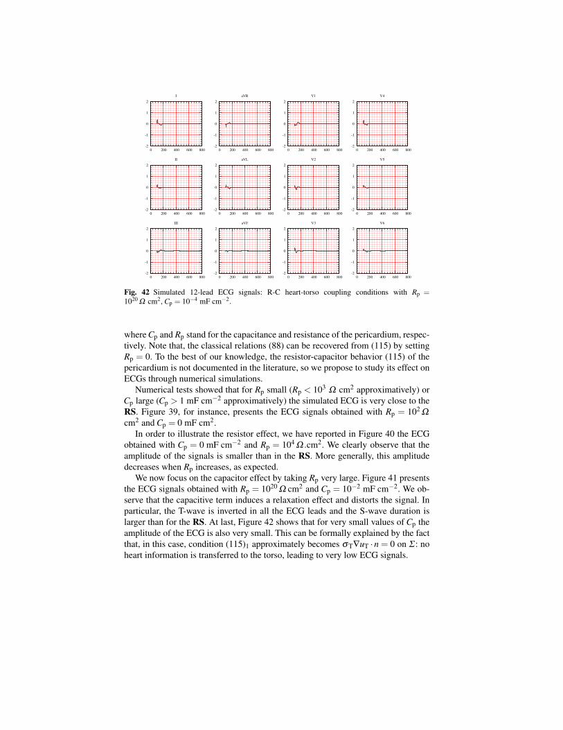
-2

-1

0

1

2

0 200 400 600 800

I

-2

-1

0

1

2

0 200 400 600 800

II

-2

-1

0

1

2

0 200 400 600 800

III

-2

-1

0

1

2

0 200 400 600 800

aVR

-2

-1

0

1

2

0 200 400 600 800

aVL

-2

-1

0

1

2

0 200 400 600 800

aVF

-2

-1

0

1

2

0 200 400 600 800

V1

-2

-1

0

1

2

0 200 400 600 800

V2

-2

-1

0

1

2

0 200 400 600 800

V3

-2

-1

0

1

2

0 200 400 600 800

V4

-2

-1

0

1

2

0 200 400 600 800

V5

-2

-1

0

1

2

0 200 400 600 800

V6

Fig. 42 Simulated 12-lead ECG signals: R-C heart-torso coupling conditions with Rp =1020 Ω cm2, Cp = 10−4 mF cm−2.

where Cp and Rp stand for the capacitance and resistance of the pericardium, respec-tively. Note that, the classical relations (88) can be recovered from (115) by settingRp = 0. To the best of our knowledge, the resistor-capacitor behavior (115) of thepericardium is not documented in the literature, so we propose to study its effect onECGs through numerical simulations.

Numerical tests showed that for Rp small (Rp < 103 Ω cm2 approximatively) orCp large (Cp > 1 mF cm−2 approximatively) the simulated ECG is very close to theRS. Figure 39, for instance, presents the ECG signals obtained with Rp = 102 Ω

cm2 and Cp = 0 mF cm2.In order to illustrate the resistor effect, we have reported in Figure 40 the ECG

obtained with Cp = 0 mF cm−2 and Rp = 104 Ω .cm2. We clearly observe that theamplitude of the signals is smaller than in the RS. More generally, this amplitudedecreases when Rp increases, as expected.

We now focus on the capacitor effect by taking Rp very large. Figure 41 presentsthe ECG signals obtained with Rp = 1020 Ω cm2 and Cp = 10−2 mF cm−2. We ob-serve that the capacitive term induces a relaxation effect and distorts the signal. Inparticular, the T-wave is inverted in all the ECG leads and the S-wave duration islarger than for the RS. At last, Figure 42 shows that for very small values of Cp theamplitude of the ECG is also very small. This can be formally explained by the factthat, in this case, condition (115)1 approximately becomes σT∇uT ·n = 0 on Σ : noheart information is transferred to the torso, leading to very low ECG signals.

6 Numerical investigations with weak heart-torso coupling

In this section, we investigate the ECG sensitivity to the time and space discretiza-tions and to the heart and torso model parameters. To carry out these studies at areasonable computational cost, we consider the heart-torso uncoupling. Althoughwe have noticed (in section 5.1) that uncoupling may affect the ECG accuracy insome cases, we can expect that the conclusions of the sensitivity analysis remainstill valid under this simplification.

6.1 Time and space convergence

In this section, we are not interested in the convergence of the whole solution of theRM with respect to the space and time discretization parameters, but rather in theconvergence of the ECG which is here considered as the quantity of interest.

6.1.1 6.1.a) Time convergence

In Figure 43, we present the first ECG lead (lead I) obtained for three different time-step sizes δ t = 0.25, 0.5 and 2 ms. The l2-norm of the relative difference with theresult obtained with δ t = 0.25 ms is 10 % when δ t = 2 ms and 2.0% when δ t = 0.5ms.

0 100 200 300 400 500 600-1

0

1

2

3

4

0.25 ms

0.5 ms

2 ms

Fig. 43 Comparison of three simulations of ECG (lead I) with three different time steps: 2, 0.5 and0.25 ms. The computation is performed using the RS parameters only the time step is changed.

6.1.2 6.1.b) Space convergence

Three different levels of refinements are considered for the heart and the torsomeshes, as shown in Table 5. The finite element meshes used in the RS are theR2. In Figure 44, we report the first lead of the ECGs obtained for these simulationsusing a time step δ t = 0.25 ms.

Meshes Heart nodes h (cm) Torso nodes Total number of tetrahedraR1 13 000 0.30 56 000 370 000R2 80 000 0.15 120 000 1 080 000R3 236 000 0.11 232 000 2 524 000

Table 5 Three different levels of refinement for the computational heart and torso meshes (roundedoff values), h denotes the discretization parameter.

0 100 200 300 400 500 600-2

-1

0

1

2

3

4 mesh 1

mesh 2

mesh 3

Fig. 44 Comparison of three simulations of ECG (lead I), using three different levels of meshrefinement (see Table 5). The computation is performed using the RS parameters only the spacediscretization parameter is changed.

Although the whole solution might not be fully converged within the heart, wecan observe that the quantity of interest – namely the ECG – is almost unaffected bythe last refinement. Therefore, in a goal-oriented refinement framework, the solutionmay indeed be considered as converged.

6.2 Sensitivity to model parameters

In this section, we study the sensitivity of ECG to some model parameters. This isfundamental step prior to addressing its estimation (see e.g. [BFGZ08a]) using dataassimilation techniques.

Suppose that α1,α2, ...,αp are parameters the ECG depends upon, i.e.

ECG = ECG(α1,α2, ...,αp).

The ECG sensitivity to parameter αi can then be approximated as

∂αiECG(α1,α2, ...,αp)≈ECG(α1,α2, ...,(1+ ε)αi, ...,αp)−ECG(α1,α2, ...,αp)

εαi,

where ε is a small parameter, in our case 10−6 ≤ ε ≤ 10−4 gives a good ap-proximation. Instead of ∂αiECG(α1,α2, ...,αp) we consider the normalized valueαi∂αiECG(α1,α2, ...,αp), which allows to compare the sensitivity irrespectively ofthe parameter scales. In the next paragraphs, we provide time evolution of this scaledderivative, evaluated around the parameters used in the RS. Once more, for the sakeof conciseness, we focus on the first ECG lead.

6.2.1 Ionic model parameters

In this paragraph, we investigate the sensitivity of the ECG to the Mitchell-Schaefferparameters. In Figure 45, we have reported the normalized derivatives with respectto τin, τout, τopen or τclose. The high ECG sensitivity to τin is clearly visible, par-ticularly during the QRS-complex. The sensitivity to τout is moderate both duringthe depolarization and depolarization phases. As expected, the sensitivity to τclose isonly relevant during repolarization. Interestingly, the sensitivity to τopen is relativelysmall. Therefore, this parameter may be removed (i.e. keep fixed) within an inverseestimation procedure.

6.2.2 Bidomain model parameters

We first focus on the ECG sensitivity to the local myocardium conductivities: σ te,

σ le, σ t

i and σ li . The corresponding normalized derivatives are given in Figure 46.

During depolarization (QRS-complex), the ECG is mainly sensitive to transverseconductivity (σ t

e, σ ti ). This can be due to the dominating transmural propagation of

the depolarization wave in the left ventricle (see Figure 19 (left)). During repolariza-tion (T-wave), on the contrary, the ECG shows approximately the same sensitivityto all the local conductivities. We now pursue our sensitivity analysis, by consider-ing the parameters Am and Cm. The corresponding normalized derivatives are givenin Figure 47. We observe a strong sensitivity to both parameters during depolariza-

0 100 200 300 400 500 600

time (ms)

-4

-2

0

2

4

6

8

tau_in

tau_out

tau_open

tau_close

!in

!out

!close

!open

Fig. 45 Normalized ECG sensitivity to τin, τout, τopen and τclose.

0 100 200 300 400 500 600

time (ms)

-2

-1

0

1

2

sigmae_l

sigmai_l

sigmae_t

sigmai_t

!le

!li

!te

!ti

Fig. 46 Normalized ECG sensitivity to the local myocardium conductivities: σ te, σ l

e, σ ti and σ l

i .

0 100 200 300 400 500 600time (ms)

-5

0

5

10

15 Am

Cm

Fig. 47 Normalized ECG sensitivity to Am and Cm.

tion. Whereas, during the repolarization phase, the sensitivity is reduced. At last,we investigate the sensitivity of the ECG to the initial activation in the heart (seeAppendix 4.1.5). More precisely, we focus on the sensitivity to the activation an-gular velocity π

2tact. The corresponding normalized derivative is reported Figure 48.

0 100 200 300 400 500 600

time (ms)

0

1

2

3

4

Fig. 48 Normalized ECG sensitivity to the activation angular velocity.

As expected, the ECG is strongly sensitive to this parameter, particularly during thedepolarization phase.

6.2.3 Torso parameters

We finally consider the sensitivity of the ECG to the torso conductivities σ lT, σb

Tand σ t

T. Note that, in a heart-torso uncoupling framework, the corresponding threenormalized derivatives are linked by a linear relation. Indeed, from (89) and (98),we have that, for all λ ∈ R, uT solves

div(λσT∇uT) = 0, in ΩT,

uT = ue, on Σ ,

λσT∇uT ·nT = 0, on Γext.

In other words,uT(λσ

lT,λσ

bT,λσ

tT) = uT(σ

lT,σ

bT,σ

tT). (116)

Differentiating this relation with respect to λ (and evaluating the resulting expres-sion at λ = 1) yields

σlT∂

σ lTuT +σ

bT∂

σbTuT +σ

tT∂σ t

TuT = 0.

Thus, from (95), we obtain a similar relation for the normalized ECG derivatives:

σlT∂

σ lTECG+σ

bT∂

σbTECG+σ

tT∂σ t

TECG = 0.

Figure 49 presents the normalized derivatives of the ECG with respect to the tis-sue, lung and bone conductivities. This figure clearly shows that the ECG sensitivityto the bone parameter σb

T is negligible compared to its sensitivity to the tissue and

0 100 200 300 400 500 600

time (ms)

-0.4

-0.2

0

0.2

0.4

sigma_tissue

sigma_lung

sigma_bones

!tT

!bT

!lT

Fig. 49 Normalized ECG sensitivity to σ lT, σb

T and σ tT.

lung parameters. Thus, if we have in mind to limit the number of parameters to beestimated, σb

T can safely be fixed to the value used in the RS.

7 Conclusion

A fully PDE/ODE based mathematical model for the numerical simulation of ECGshas been described. The electrical activity of the heart is based on the coupling ofthe bidomain equations with the Mitchell-Schaeffer phenomenological ionic model,including anisotropic conductivities and transmural APD heterogeneity. This sys-tem of equations has been coupled to a generalized Laplace equation in the torso,with inhomogeneous conductivity (bone, lungs and remaining tissue). A detailed de-scription of the different algorithms used for the numerical solution of the resultingECG model has been also provided.

Our approach has several limitations: we did not consider the atria, which pre-vents us from computing the P wave of the ECG; the cell model being phenomeno-logical, it cannot handle complex ionic interactions; the effect of the blood flow onthe ECG was neglected; the geometry of the ventricles were simplified.

Despite the above mentioned limitations, we were able to compute a satisfac-tory healthy 12-lead ECG, with a limited number a parameters. To the best of ourknowledge, this constitutes a breakthrough in the modeling of ECGs with partial dif-ferential equations. Moreover, for pathological situations corresponding to a bundlebranch block and arrhythmia, our simulations have provided ECGs which satisfytypical criteria used by medical doctors to detect these pathologies. This shows, inparticular, that our numerical model have some predictive features.

In a second part, we have studied the impact of some modeling assumptions onthe ECGs. The main conclusions of this investigation are the following:

1. As far as the general shape of the ECGs is concerned, heart-torso uncouplingcan be considered. The level of accuracy obtained with uncoupling is probably

sufficient in several applications, which may explain why this simplification isso widespread in the literature. Nevertheless, our numerical results have clearlypointed out that the amplitudes of the ECG signals obtained via uncoupling andfull coupling can significantly differ. We therefore recommend to carefully checkin each specific situations whether the uncoupling approximation is acceptable ornot.

2. In agreement with other studies, we noticed that cell heterogeneity and fiberanisotropy have an important impact on the ECG and, therefore, cannot be ne-glected.

3. The bidomain equations can apparently be safely replaced by the monodomainequations without significantly affecting the ECG. Nevertheless, even with thissimplification, we point out that the transmembrane potential Vm and the extra-cellular potential ue still have to be solved simultaneously when the heart and thetorso are fully coupled. To be really attractive, the monodomain simplificationhas therefore to come with the uncoupling approximation, which can affect theECG, as mentioned above.

4. We have proposed a new heart-torso coupling condition which takes into accountpossible capacitive and resistive effects of the pericardium. We did not find in theliterature any evidence of these effects and our results show that it does not seemnecessary to include them in order to get realistic healthy ECGs. Nevertheless,these coupling conditions might be relevant in some pathologies affecting thepericardial sac and the simulations we provided to illustrate these effects mightbe useful for future works.

5. At last, a sensitivity analysis has shown that the most critical parameters of thebidomain model are Cm, Am, the angular velocity of the activation wave and thetransverse conductivities σ t

i and σ te. As regards the ECG sensitivity to the ionic

model parameters, we have noticed a extreme sensitivity of the QRS-complexto the parameter τin and a high sensitivity of the T-wave to the parameter τclose.Moreover, we have also observed that the ECG sensitivity to the torso conduc-tivity parameters is less significant than to the heart model parameters.

To conclude, our main concern during this study was to build a model rich enoughto provide realistic ECGs and simple enough to be easily parametrized. In spite ofits shortcomings, the proposed approach essentially fulfills these requirements andis therefore a good candidate to address inverse problems. This will be investigatedin future works.

Chapter 6Decoupled time-marching schemes incomputational cardiac electrophysiology andECG numerical simulation

In order to decouple the computation of the unknown fields (ionic state, transmem-brane potential, extracellular and torso potentials) in both isolated heart problem(18) and heart-torso problem (24)-(26), we propose in this chapter first order semi-implicit time-marching schemes and a Robin-Robin treatment of the heart-torsocoupling conditions. For the isolated bidomain system, we show that the Gauss-Seidel and Jacobi like splittings do not compromise energy stability; they simplyalter the energy norm. Time-step constraints are only due to the semi-implicit treat-ment of the non-linear reaction terms. Within the framework of the numerical sim-ulation of electrocardiograms (ECG), these bidomain splittings are combined withan explicit Robin-Robin treatment of the heart-torso coupling conditions. We showthat the resulting schemes allow a fully decoupled (energy) stable computation ofthe heart and torso fields, under an additional mild CFL like condition. Numericalsimulations, based on anatomical heart and torso geometries, illustrate the stabilityand accuracy of the proposed schemes.

This chapter is part of a joint work with M.A. Fernández, it is reported in [FZ09].

1 Introduction

Computational models of cardiac electrophysiology typically incorporate the cellmembrane activity and the intra- and extracellular components of cardiac tissueby means of the bidomain model (see e.g. [SLC+06, PBC05]). This mathemati-cal model can be formulated as a three-field system (ionic state, transmembrane andextracellular potentials) coupling a non-linear reaction-diffusion equation, an ellip-tic equation and a non-linear system of ODE (alternative formulations are discussedin [HHLR94, PS02]).

The rapid dynamics of the ODE system, acting on the reaction terms, lead tothe presence of a sharp propagating wavefront, which often requires fine resolu-tions in space and in time. As a result, fully implicit time-marching is extremelydifficult to perform since it involves the resolution of a large system of non-linear

105

equations at each time step (see e.g. [HHLR94, BEL03, MC04, MP09]). Attemptsto reduce this computational complexity (without compromising too much numeri-cal stability) consist in introducing some sort of explicit treatment within the time-marching procedure. For instance, by considering semi-implicit described in chap-ter 5 (see e.g. [SLT01, LGT03, CFP04, ATP06, BFGZ07, EB08a]) or operatorsplitting (see e.g. [KB98, SLT05, VWdSP+08]) schemes. All these approaches un-couple the ODE system (ionic state and non-linear reaction terms) from the elec-trodiffusive components (transmembrane and extracellular potentials). Other works[SLT01, LGT03, ATP06, VWdSP+08, PDR+06] propose a decoupled (Gauss-Seidel like) time-marching of the three fields.

In this chapter we go further in the investigation of this kind of decoupling tech-niques, by providing a general energy based stability analysis that covers both theGauss-Seidel and the Jacobi like approaches. In particular, we show that these elec-trodiffusive splittings do not compromise the stability of the resulting scheme. Theysimply alter the energy norm and time step restrictions are uniquely dictated by thesemi-implicit treatment of the ODE system and the non-linear reaction terms.

In the second part, we propose to extend these time-marching techniques to thenumerical simulation of the ECG, namely, the forward problem of cardiac elec-trophysiolgy (see e.g. [LBG+03]). The bidomain equations have then to be cou-pled to a generalized Laplace equation, describing the electrical potential withinthe surrounding torso tissue. The heart-torso coupling is enforced through stan-dard interface conditions, ensuring a perfect electrical balance (see e.g. [KN94,PBC05, SLC+06]). This results in a coupled four-field problem (ionic state, trans-membrane, extracellular and torso potentials) coupling a non-linear system ofODEs, a non-linear reaction-diffusion equation and two elliptic equations (see e.g.[LBG+03, SLC+06]).

Traditionally, the heart-torso coupling has been treated using two different ap-proaches (see e.g. [LBG+03]). The so called heart-torso uncoupling approximation(see Chapter 5 section 5.1 or [PDG03, LBG+03, BCF+09]) uncouples the heart andtorso problems by neglecting the torso-to-heart electrical feedback (i.e. the heartis isolated). Although this approach is very appealing in terms of computationalcost, it can compromise the accuracy of the corresponding ECG signals (see e.g.[LBG+03, PBC05, BCF+09]). The second approach, the so called heart-torso fullcoupling, treats the heart-torso interface conditions in a fully implicit fashion and,therefore, requires the resolution of a large heart-torso system at each time step (seee.g. [SLT01, LGT03, PBC05, BCF+09]). To the best of our knowledge, none of thecurrent approaches is able to provide accurate ECG signals (i.e. close to heart-torsofull coupling) with a decoupled computation of the extracellular and torso poten-tials.

In this chapter, we introduce a series of time-marching schemes for ECG numer-ical simulation involving a fully decoupled computation of the ionic state, the trans-membrane potential, the extracellular potential and the torso potential. The mainidea consists in combining the above mentioned Gauss-Seidel or Jacobi like bido-main splittings, with an explicit Robin-Robin treatment (derived from [ACF09]) ofthe heart-torso coupling. An energy based stability analysis shows that the proposed

schemes are stable under and additional mild CFL like condition. Note that, since thetime discretization of the two (quasi-static) elliptic equations does not produce nu-merical dissipation, conventional explicit Dirichlet-Neumann heart-torso couplingmight lead to numerical instability.

The remainder of this chapter is organized as follows. In the next section webriefly recall the coupled system of equations describing the electrical activity ofthe heart and its interaction with the surrounding torso tissue. The time discretiza-tion of the bidomain equations is addressed in section §3, using Gauss-Seidel andJacobi like eletrodiffusive splittings. The stability of the resulting schemes is ana-lyzed by means of energy arguments. Section §4 is devoted to the discretization ofthe heart-torso system. The schemes analyzed in section §3 are then combined witha specific explicit Robin-Robin treatment of the heart-torso coupling. The energybased stability of the resulting schemes is investigated. Numerical evidence is pro-vided in section §5, using realistic heart and torso geometries. A summary of theresults and some concluding remarks are given in section §6.

2 Mathematical models

This section contains standard material (see e.g. [SLC+06, Chapter 2]). We intro-duce the notation and the coupled system of equations commonly used to model theelectrical activity of the heart and its interaction with surrounding tissue (extramy-ocardial regions).

2.1 Isolated heart

The bidomain equations, originally derived in [Tun78], are the most widely acceptedmathematical model of the macroscopic electrical activity of the heart (see e.g. themonographs [SLC+06, PBC05]). This model is usually formulated in terms of threevariables: the transmembrane potential Vm, the extracellular potential ue and theionic state w (possibly vector valued). These space and time dependent variables aredefined in ΩH× (0,T ), where ΩH and (0,T ) denote, respectively, the heart domainand the time interval of interest.

The governing equations consist of a coupled system of ODE, a nonlinearreaction-diffusion equation and an elliptic equation, with appropriate boundary andinitial conditions (see e.g. [SLC+06, PBC05]):

∂tw+g(Vm,w) = 0, in ΩH× (0,T ),(117)

χm∂tVm + Iion(Vm,w)−div(σ i∇Vm)−div(σ i∇ue) = Iapp, in ΩH× (0,T ),(118)

−div((σ i +σ e)∇ue)−div(σ i∇Vm) = 0, in ΩH× (0,T ),(119)

σ i∇Vm ·n+σ i∇ue ·n = 0, on Σ × (0,T ),(120)

σ e∇ue ·n = 0, on Σ × (0,T ),(121)

Vm(x,0) =V 0m(x), w(x,0) = w0(x), ∀x ∈ΩH. (122)

Here, χmdef= AmCm where Am is a geometrical quantity, Cm denotes the membrane

capacitance and tensors σ i and σ e represent, respectively, the intra- and extracel-lular conductivities. The term Iion(Vm,w)

def= Amiion(Vm,w) denotes the ionic current

across the membrane and Iapp a given external current stimulus. The explicit expres-sion of functions g and iion depends on the considered cell ionic model (see e.g.[SLC+06, PBC05] and the references therein). At last, n stands for the outward unitnormal to Σ

def= ∂ΩH (see Figure 50), and V 0

m, w0 are given initial data.The boundary conditions (120)-(121) state that the intra- and extracellular cur-

rents do not propagate outside the heart. While (120) is a widely accepted condi-tion (see e.g. [Tun78, KN94, PBC05, SLC+06]), the enforcement of (121) is onlyjustified under an isolated heart assumption (see [SLC+06, PBC05]). The coupledsystem of equations (117)-(122) is often known in the literature as isolated bido-main model (see e.g. [CFP04, CFP04, SLC+06]). The interested reader is referredto [CFS02, BK06, BCP09, Ven09] for the mathematical analysis of problem (117)-(122).

The choice of the formulation (117)-(122) is motivated by the decoupling time-marching schemes introduced in section §3. Other formulations of the bidomainequations and their impact on the performance of the algebraic solvers have beendiscussed in [HHLR94, PS02]. A recent review of numerical methods for the bido-main equations can be found in [LSH+09].

Remark 1. The complexity of (117)-(122) can be reduced by using, instead of (118)and (120), the so-called monodomain approximation:

χm∂tVm + Iion(Vm,w)−div(σ∇Vm

)= Iapp, in ΩH,

σ∇Vm ·n = 0, on Σ ,(123)

where σdef= σ i(σ i + σ e)

−1σ e is the bulk conductivity tensor (see e.g. [LH91,CNLH04, CFP04, PDR+06]). Note that (123) decouples de computation of Vm fromthat of ue. Under the isolating condition (121), (123) can be interpreted as the zeroth-

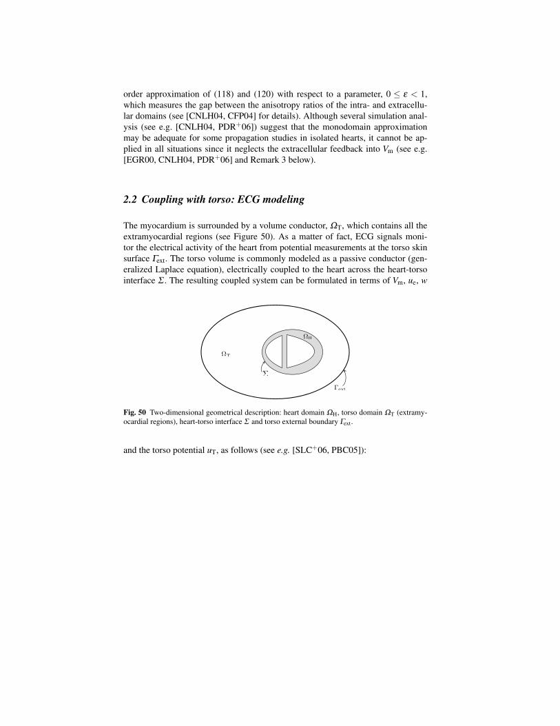
order approximation of (118) and (120) with respect to a parameter, 0 ≤ ε < 1,which measures the gap between the anisotropy ratios of the intra- and extracellu-lar domains (see [CNLH04, CFP04] for details). Although several simulation anal-ysis (see e.g. [CNLH04, PDR+06]) suggest that the monodomain approximationmay be adequate for some propagation studies in isolated hearts, it cannot be ap-plied in all situations since it neglects the extracellular feedback into Vm (see e.g.[EGR00, CNLH04, PDR+06] and Remark 3 below).

2.2 Coupling with torso: ECG modeling

The myocardium is surrounded by a volume conductor, ΩT, which contains all theextramyocardial regions (see Figure 50). As a matter of fact, ECG signals moni-tor the electrical activity of the heart from potential measurements at the torso skinsurface Γext. The torso volume is commonly modeled as a passive conductor (gen-eralized Laplace equation), electrically coupled to the heart across the heart-torsointerface Σ . The resulting coupled system can be formulated in terms of Vm, ue, w

!T

!H

!ext

!

Fig. 50 Two-dimensional geometrical description: heart domain ΩH, torso domain ΩT (extramy-ocardial regions), heart-torso interface Σ and torso external boundary Γext.

and the torso potential uT, as follows (see e.g. [SLC+06, PBC05]):

∂tw+g(Vm,w) = 0, in ΩH× (0,T ),(124)

χm∂tVm + Iion(Vm,w)−div(σ i∇Vm)−div(σ i∇ue) = Iapp, in ΩH× (0,T ),(125)

−div((σ i +σ e)∇ue)−div(σ i∇Vm) = 0, in ΩH× (0,T ),(126)

−div(σT∇uT) = 0, in ΩT× (0,T ),(127)

σT∇uT ·nT = 0, on Γext× (0,T ),(128)

σ i∇Vm ·n+σ i∇ue ·n = 0, on Σ × (0,T ),(129)

uT = ue, on Σ × (0,T ),(130)

σ e∇ue ·n =−σT∇uT ·nT, on Σ × (0,T ),(131)

Vm(x,0) =V 0m(x), w(x,0) = w0(x), ∀x ∈ΩH. (132)

Here, σT stands for the conductivity tensor of the torso tissue and nT for the outwardunit normal to the external boundary Γext

def= ∂ΩT \Σ (see Figure 50).

The boundary condition (128) states that no current can flow from the externaltorso surface Γext, whereas (130)-(131) enforce a perfect electric balance betweenthe heart and torso domains (see e.g. [Tun78, KN94, PBC05, SLC+06]).

The coupled system of equations (124)-(132) is often known in the literature asfull bidomain or coupled bidomain model (see e.g. [CNLH04, SLC+06]). It canbe considered as the state-of-the-art in the modeling of the ECG or, equivalently,the forward problem of cardiac electrophysiology (see e.g. [LBG+03, PBC05,SLC+06]). The interested reader is referred to chapter 4 or [BFGZ08b] for themathematical analysis of problem (124)-(132), and to [LBG+03] (see also Chap-ter 5 section 3) for a review of the numerical methods.

Remark 2. A common approach to reduce the computational complexity of (124)-(132) consists in uncoupling the computation of (w,Vm,ue) and uT, by neglectingthe electrical torso-to-heart feedback (see e.g. [CNLH04, PDG03, LBG+03]). Thus,the coupling condition (131) is replaced by

σ e∇ue ·n = 0, on Σ , (133)

which amounts to work with an isolated bidomain model, as described in the previ-ous subsection. Thereafter, the torso potential uT is recovered by solving (127) withboundary conditions (128)-(130). Although this approach is very appealing in termsof computational cost, numerical evidence has shown that it can compromise the

accuracy of the ECG signals (see e.g. [LBG+03, PBC05, BCF+09] and the numer-ical study of subsection §5.3). The heart-torso uncoupling approximation is oftenfurther simplified by replacing the interface condition (130) by a (multi-) dipolerepresentation of the cardiac source (see e.g. [Gul88, Hui98]).

Remark 3. The monodomain approximation (123) can be combined with the heart-torso uncoupling framework of Remark 2 (see e.g. [Hui98, PDG03, BCF+09]). Thisyields a simplified mathematical model which allows a fully decoupled computationof Vm, ue and uT. However, as noticed in Chapter 5 section 5.2 (see also [CNLH04]),without the uncoupling assumption (133) the monodomain approximation becomes

χm∂tVm + Iion(Vm,w)−div(σ∇Vm

)= Iapp, in ΩH,

σ∇Vm ·n =−µσ e∇ue ·n, on Σ ,(134)

where 0 < µ < 1 is a dimensionless parameter related to the local conductivities.Note that in (134) Vm and ue are still coupled. Therefore, under the full heart-torsocoupling (130)-(131), the monodomain approximation does not reduce the compu-tational complexity with respect to (124)-(132).

3 Decoupled time-marching for the bidomain equation

In this section we analyze some time-discretization schemes for the isolated bido-main system (117)-(122). The main feature of the analyzed schemes is that they allallow a decoupled (Gauss-Seidel or Jacobi like) computation of Vm and ue, withoutcompromising stability.

3.1 Preliminaries

In what follows, we will consider the usual Lebesgue and Sobolev spaces, Lm(Ω)and Hm(Ω) respectively (m > 0), for a domain Ω ⊂ R3. Then, for a given X ⊂ ∂Ω

(with meas(X) > 0), we define H1X (Ω) as the subspace of H1(Ω) with vanishing

trace on X . The L2(Ω)-norm is denoted by ‖ · ‖0,Ω and the vanishing mean valuesubspace of L2(Ω) by L2

0(Ω).Problem (117)-(122) can be cast into weak form as in chapter 4 (see e.g.

[BFGZ08b]): for t > 0, find w(·, t) ∈ L∞(ΩH), Vm(·, t) ∈ H1(ΩH) and ue(·, t) ∈H1(ΩH)∩L2

0(ΩH), such that

∫

ΩH

(∂tw+g(Vm,w)

)ξ = 0,

χm

∫

ΩH

(∂tVm + Iion(Vm,w)

)φ +

∫

ΩH

σ i∇(Vm +ue) ·∇φ =

∫

ΩH

Iappφ ,

∫

ΩH

(σ i +σ e)∇ue ·∇ψ +

∫

ΩH

σ i∇Vm ·∇ψ = 0,

(135)

for all (ξ ,φ ,ψ) ∈ L2(ΩH)×H1(ΩH)×(H1(ΩH)∩L2

0(ΩH)).

3.2 Time semi-discrete formulations: decoupled time-marchingschemes

Let N ∈ N∗ be a given integer and consider a uniform partition [tn, tn+1]0≤n≤N−1,

with tndef= nτ , of the time interval of interest (0,T ), with time-step τ

def= T/N. For a

given time dependent function X , the quantity Xn denotes an approximation of X(tn)

and Dτ Xn def= (Xn−Xn−1)/τ the first order backward difference. Moreover, we set

Inapp

def= Iapp(tn, ·).

We propose to time semi-discretize (135) by combining a first order semi-implicittreatment of the ionic current evaluation with an explicit (Gauss-Seidel or Jacobilike) treatment of the coupling between Vm and ue. The resulting schemes can becast into a common frame as follows: For 0≤ n≤ N−1, we solve

1. Ionic state: find wn+1 ∈ L∞(ΩH) such that∫

ΩH

(Dτ wn+1 +g(V n

m,wn+1)

)ξ = 0 (136)

for all ξ ∈ L2(ΩH).2. Transmembrane potential: find V n+1

m ∈ H1(ΩH) such that

χm

∫

ΩH

DτV n+1m φ +

∫

ΩH

σ i∇V n+1m ·∇φ

+

∫

ΩH

σ i∇u?e ·∇φ =

∫

ΩH

(In+1app − Iion(V n

m,wn+1)

)φ (137)

for all φ ∈ H1(ΩH).3. Extracellular potential: find un+1

e ∈ H1(ΩH)∩L20(ΩH),

∫

ΩH

(σ i +σ e)∇un+1e ·∇ψ +

∫

ΩH

σ i∇V ?m ·∇ψ = 0 (138)

for all ψ ∈ H1(ΩH)∩L20(ΩH).

Note that the non-linear system (136) and the ionic current evaluation Iion(V nm,w

n+1)in (137) are decoupled from (137)-(138). This semi-implicit treatment is quite pop-ular in the literature (see e.g. [SLT01, LGT03, CFP04, ATP06, BFGZ07, EB08a]).For (u?e ,V

?m)= (un+1

e ,V n+1m ), the unknown potentials V n+1

m and un+1e are implicit cou-

pled and, therefore, equations (137) and (138) have to be solved simultaneously (seee.g. [KB98, SLT05, EB08a, EB08a, BCF+09]). The energy based stability analysisof this semi-implicit scheme, using first and second order time discretizations, hasbeen recently reported in [EB08a].

On the contrary, for (u?e ,V?m) = (un

e ,Vn+1m ) or (u?e ,V

?m) = (un

e ,Vnm), the electrodif-

fusive coupling becomes explicit and therefore (137) and (138) can be solved sep-arately: either sequentially (Gauss-Seidel) or in parallel (Jacobi). Similar Gauss-Seidel like splittings have been proposed and successfully applied in [SLT01,LGT03, ATP06, VWdSP+08]. The theoretical stability of the schemes is, however,not established therein. To the best of our knowledge, the Jacobi like splitting hasnot yet been considered in the literature.

The energy based stability analysis of these time splitting schemes is performedin the next subsection.

Remark 4. The Gauss-Seidel and Jacobi like electrodiffusive splittings allow a de-coupled computation of Vm and ue without the need to resort to monodomain ap-proximations (see Remark 1).

3.3 Stability analysis

For the stability analysis below, we shall make use of the following simplifyingassumption (see [EB08a, Section 3.2.2] and Remark 3.1 therein) on the structure ofthe ionic functions g and Iion:

Iion(Vm,w)≤CI(|Vm|+ |w|

),

g(Vm,w)≤Cg(|Vm|+ |w|

) (139)

for all Vm,w, and we set αdef= 1+3CI +Cg and β

def= CI +3Cg.

The next theorem states the energy based stability of the time-marching schemes(136)-(138), in terms of u?e and V ?

m.

Theorem 1. Assume that (139) holds and that the conductivity tensors σ i,σ e aresymmetric and positive-definite. Let (wn,V n

m,une)N

n=0 be solution of (136)-(138)

and C(T,α,β )def= exp

(T/(1− τ maxα,β)

). Then, under the condition

τ <1

maxα,β , (140)

there follows:

• For (u?e ,V?m) = (un+1

e ,V n+1m ):

∥∥wn∥∥20,ΩH

+χm∥∥V n

m∥∥2

0,ΩH+2

n−1∑

m=0

τ∥∥σ

12e ∇um+1

e∥∥2

0,ΩH+2

n−1∑

m=0

τ∥∥σ

12i ∇(V m+1

m +um+1e )

∥∥20,ΩH

≤C(T,α,β )

(∥∥w0∥∥2

0,ΩH+χm

∥∥V 0m∥∥2

0,ΩH+

n−1∑

m=0

τ∥∥Im+1

app∥∥2

0,ΩH

), (141)

with 1≤ n≤ N.• For (u?e ,V

?m) = (un

e ,Vn+1m ):

∥∥wn∥∥20,ΩH

+χm∥∥V n

m∥∥2

0,ΩH+ τ∥∥σ

12i ∇un

e∥∥2

0,ΩH

+2n−1∑

m=0

τ∥∥σ

12e ∇um+1

e∥∥2

0,ΩH+

n−1∑

m=0

τ∥∥σ

12i ∇(V m+1

m +um+1e )

∥∥20,ΩH

≤C(T,α,β )

(∥∥w0∥∥2

0,ΩH+χm

∥∥V 0m∥∥2

0,ΩH+ τ∥∥σ

12i ∇u0

e∥∥2

0,ΩH+

n−1∑

m=0

τ∥∥Im+1

app∥∥2

0,ΩH

),

(142)

with 1≤ n≤ N.• For (u?e ,V

?m) = (un

e ,Vnm):

∥∥wn∥∥20,ΩH

+χm∥∥V n

m∥∥2

0,ΩH+ τ∥∥σ

12i ∇un

e∥∥2

0,ΩH+ τ∥∥σ

12i ∇V n

m∥∥2

0,ΩH

+2n−1∑

m=0

τ∥∥σ

12e ∇um+1

e∥∥2

0,ΩH≤C(T,α,β )

(∥∥w0∥∥20,ΩH

+χm∥∥V 0

m∥∥2

0,ΩH+ τ∥∥σ

12i ∇V 0

m∥∥2

0,ΩH

+τ∥∥σ

12i ∇u0

e∥∥2

0,ΩH+

n−1∑

m=0

τ∥∥Im+1

app∥∥2

0,ΩH

), (143)

with 1≤ n≤ N.

Proof. Under assumptions (139) and (140), the stability estimate (141), for themonolithic case (u?e ,V

?m) = (un+1

e ,V n+1m ), can be straightforwardly derived from the

analysis reported in [EB08a] (see also [Tho06a]). Therefore, we only detail here theproofs of (142) and (143).

Let first consider the Gauss-Seidel like decoupling (u?e ,V?m)= (un

e ,Vn+1m ). By test-

ing (136)-(138) with τ(wn+1,V n+1m ,un+1

e ) and after summation of the resulting ex-pressions we have:

12

(∥∥wn+1∥∥20,ΩH−∥∥wn∥∥2

0,ΩH

)+

χm

2

(∥∥V n+1m∥∥2

0,ΩH−∥∥V n

m∥∥2

0,ΩH

)+τ∥∥σ

12e ∇un+1

e∥∥2

0,ΩH

+ τ∥∥σ

12i ∇(V n+1

m +un+1e )

∥∥20,ΩH

+ τ

∫

ΩH

σ i∇(une−un+1

e ) ·∇V n+1m

︸︷︷︸I1

≤ τ

∫

ΩH


m,wn+1)

)V n+1

m − τ

∫

ΩH

g(V nm,w

n+1))wn+1

︸︷︷︸I2

, (144)

where the square roots σ12e ,σ

12i are well defined since σ i,σ e are symmetric and

positive-definite tensors (see e.g. [Ste80]). We now provide appropriate bounds forterms I1 and I2.

As regards the first term, we have

I1 =τ

∫

ΩH

σ i∇(une−un+1

e ) ·∇(V n+1m +un+1

e )+

∫

ΩH

σ i∇(un+1e −un

e) ·∇un+1e

≥− τ

2

∥∥σ12i ∇(un

e−un+1e )

∥∥20,ΩH− τ

2

∥∥σ12i ∇(V n+1

m +un+1e )

∥∥20,ΩH

+τ

2

(∥∥σ12i ∇un+1

e∥∥2

0,ΩH−∥∥σ

12i ∇un

e∥∥2

0,ΩH

)+

τ

2

∥∥σ12i ∇(un+1

e −une)∥∥2

0,ΩH

=τ

2

(∥∥σ12i ∇un+1

e∥∥2

0,ΩH−∥∥σ

12i ∇un

e∥∥2

0,ΩH

)− τ

2

∥∥σ12i ∇(V n+1

m +un+1e )

∥∥20,ΩH

.

(145)On the other hand, from (139), for the second term can be bounded as follows

I2 =τ

2

∥∥In+1app∥∥2

0,Ω 2H+

τ

2

∥∥V n+1m∥∥2

0,ΩH+

τCI

2

(3∥∥V n+1

m∥∥2

0,ΩH+∥∥wn+1∥∥2

0,ΩH

)

+τCg

2

(∥∥V n+1m∥∥2

0,ΩH+3∥∥wn+1∥∥2

0,ΩH

)

=τ

2


0,ΩH+

τ

2(1+3CI +Cg)︸︷︷︸

α

∥∥V n+1m∥∥2

0,ΩH+

τ

2(CI +3Cg)︸︷︷︸

β

∥∥wn+1∥∥20,ΩH

.

(146)As a result, inserting (145) and (146) into (144), yields

12

(∥∥wn+1∥∥20,ΩH−∥∥wn∥∥2

0,ΩH

)+

χm

2

(∥∥V n+1m∥∥2

0,ΩH−∥∥V n

m∥∥2

0,ΩH

)+τ∥∥σ

12e ∇un+1

e∥∥2

0,ΩH

+τ

2

∥∥σ12i ∇(V n+1

m +un+1e )

∥∥20,ΩH

+τ

2

(∥∥σ12i ∇un+1

e∥∥2

0,ΩH−∥∥σ

12i ∇un

e∥∥2

0,ΩH

)

≤ τ

2


0,ΩH+

τα

2

∥∥V n+1m∥∥2

0,ΩH+

τβ

2

∥∥wn+1∥∥20,ΩH

,

so that, replacing index n by m and summing over 0≤ m≤ n−1, we have

∥∥wn∥∥20,ΩH

+χm∥∥V n

m∥∥2

0,ΩH+ τ∥∥σ

12i ∇un

e∥∥2

0,ΩH+2

n−1∑

m=0

τ∥∥σ

12e ∇um+1

e∥∥2

0,ΩH

+

n−1∑

m=0

τ∥∥σ

12i ∇(V m+1

m +um+1e )

∥∥20,ΩH≤∥∥w0∥∥2

0,ΩH+χm

∥∥V 0m∥∥2

0,ΩH+ τ∥∥σ

12i ∇u0

e∥∥2

0,ΩH

+

n−1∑

m=0

τ∥∥Im+1

app∥∥2

0,ΩH+α

n−1∑

m=0

τ∥∥V m+1

m∥∥2

0,ΩH+β

n−1∑

m=0

τ∥∥wm+1∥∥2

0,ΩH.

Estimate (142) then follows by applying Gronwall’s lemma (see e.g. [HR90a,Lemma 5.1]) under condition (140).

Finally, let consider the Jacobi like decoupling (u?e ,V?m) = (un

e ,Vnm). In this case,

estimate (144) becomes

12

(∥∥wn+1∥∥20,ΩH−∥∥wn∥∥2

0,ΩH

)+

χm

2

(∥∥V n+1m∥∥2

0,ΩH−∥∥V n

m∥∥2

0,ΩH

)+τ∥∥σ

12e ∇un+1

e∥∥2

0,ΩH

+ τ∥∥σ

12i ∇(V n+1

m +un+1e )

∥∥20,ΩH

+ I1 + τ

∫

ΩH

σ i∇(V nm−V n+1

m ) ·∇un+1e

︸︷︷︸I3

≤ I2. (147)

The new term I3 can be bounded similarly to I1, that is,

I3 =τ

∫

ΩH

σ i∇(V nm−V n+1

m ) ·∇(V n+1m +un+1

e )+

∫

ΩH

σ i∇(V n+1m −V n

m) ·∇V n+1m

≥− τ

2

∥∥σ12i ∇(V n

m−V n+1m )

∥∥20,ΩH− τ

2

∥∥σ12i ∇(V n+1

m +un+1e )

∥∥20,ΩH

+τ

2

(∥∥σ12i ∇V n+1

m∥∥2

0,ΩH−∥∥σ

12i ∇V n

m∥∥2

0,ΩH

)+

τ

2

∥∥σ12i ∇(V n+1

m −V nm)∥∥2

0,ΩH

=τ

2

(∥∥σ12i ∇V n+1

m∥∥2

0,ΩH−∥∥σ

12i ∇V n

m∥∥2

0,ΩH

)− τ

2

∥∥σ12i ∇(V n+1

m +un+1e )

∥∥20,ΩH

.

(148)Therefore, by inserting (145), (146) and (148) into (147), there follows that

12

(∥∥wn+1∥∥20,ΩH−∥∥wn∥∥2

0,ΩH

)+

χm

2

(∥∥V n+1m∥∥2

0,ΩH−∥∥V n

m∥∥2

0,ΩH

)+τ∥∥σ

12e ∇un+1

e∥∥2

0,ΩH

τ

2

(∥∥σ12i ∇V n+1

m∥∥2

0,ΩH−∥∥σ

12i ∇V n

m∥∥2

0,ΩH

)+

τ

2

(∥∥σ12i ∇un+1

e∥∥2

0,ΩH−∥∥σ

12i ∇un

e∥∥2

0,ΩH

)

≤ τ

2


0,ΩH+

τα

2

∥∥V n+1m∥∥2

0,ΩH+

τβ

2

∥∥wn+1∥∥20,ΩH

.

Estimate (143) then holds, under condition (140), by replacing index n by m, sum-ming over 0≤m≤ n−1 and applying Gronwall’s lemma. This completes the proof.

We conclude this section with a series of remarks.

Remark 5. Theorem 1 shows that electrodiffusive Gauss-Seidel and Jacobi split-tings are energy stable under condition (140), as for the unsplit case (u?e ,V

?m) =

(un+1e ,V n+1

m ) (analyzed in [EB08a]), but with slightly altered energy norms. As aresult, stability is not compromised.

Remark 6. The proof of Theorem 1 does not depend on the time discretizations con-sidered in (136) and (137). Indeed, we do not make use of any numerical dissipationproduced by the scheme, apart from that is directly provided by the splitting. There-fore, the backward Euler quotients, Dτ wn+1 and DτV n+1

m , can be safely replaced bya second order backward difference formula, and perform one correction (see e.g.[Ste78, SM00]) to recover overall second order accuracy.

Remark 7. The above stability result can be adapted, with minor modifications, tothe case (u?e ,V

?m) = (un+1

e ,V nm). The full Jacobi splitting, obtained after replacing

Iion(V nm,w

n+1) by Iion(V nm,w

n) in (137) could also be considered.

Remark 8. Theorem 1 holds also for the fully discrete counterpart of (136)-(138)obtained by discretizing in space using finite elements (see subsection §4.1).

4 Decoupled time-marching for ECG numerical simulation

In this section, we introduce fully discrete schemes for the heart-torso system (124)-(132), allowing a decoupled computation of the transmembrane, extracellular andtorso potentials. The main idea consists in combining the bidomain splittings of theprevious section, with a specific explicit Robin-Robin treatment of the heart-torsocoupling conditions (130)-(131).

4.1 Preliminaries

Problem (124)-(132) can be cast into weak form as follows (see e.g. [BFGZ08b]):for t > 0, find w(·, t)∈ L∞(ΩH), Vm(·, t)∈H1(ΩH), ue(·, t)∈H1(ΩH)∩L2

0(ΩH) anduT(·, t) ∈ H1(ΩT) with ue(·, t) = uT(·, t) on Σ , such that

∫

ΩH

(∂tw+g(Vm,w)

)ξ = 0,

χm

∫

ΩH

(∂tVm + Iion(Vm,w)

)φ +

∫

ΩH

σ i∇(Vm +ue) ·∇φ =

∫

ΩH

Iappφ ,

∫

ΩH

(σ i +σ e)∇ue ·∇ψ +

∫

ΩH

σ i∇Vm ·∇ψ +

∫

ΩT

σT∇uT ·∇ζ = 0,

(149)for all (ξ ,φ ,ψ,ζ )∈ L2(ΩH)×H1(ΩH)×

(H1(ΩH)∩L2

0(ΩH))×H1(ΩT) with ψ =

ζ on Σ .

Assume that ΩH and ΩT are polygonal domains and let TH,h0<h≤1 (TT,h0<h≤1)be a family of triangulations of ΩH (resp. ΩT) satisfying the usual requirements offinite element approximations (see e.g. [EG04]). The subscript h ∈ (0,1] refer tothe level of refinement of the triangulations. For the sake of simplicity and withoutloss of generality, we assume that both families of triangulations are quasi-uniformand that they match at the heart-torso interface Σ . We define XH,h (resp. XT,h) asan internal continuous Lagrange finite element approximation of H1(ΩH) (resp.H1(ΩT)). We also introduce the standard finite element (heart-to-torso) lifting oper-ator Lh : XH,h→ XT,h∩H1

Γext(ΩT), such that Lhψ = ψ on Σ and Lhψ = 0 on Γext,

for all ψ ∈ XH,h. Note that we have the direct sum decomposition

(ψ,ζ )∈XH,h×XT,h : ψ|Σ = ζ|Σ

=(

ψ,Lhψ)

: ψ ∈XH,h⊕(0,ζ ) : ζ ∈XT,h∩H1

Σ (ΩT).

(150)In the stability analysis below, we shall make use of the following standard discretetrace-inverse inequality (see e.g. [Tho06a]):

||v||20,∂K ≤Cti

h||v||20,K ∀v ∈ XT,h, (151)

for all K ∈ TT,h, and with Cti > 0 a constant independent of the discretization pa-rameter h (but that might depend on the polynomial order).

By combining the semi-implicit time-marching schemes of section §3 with afinite element discretization in space, we can derive from (149) the following fullydiscrete heart-torso scheme: for 0 ≤ n ≤ N − 1, find wn+1 ∈ XH,h, V n+1

m ∈ XH,h,un+1

e ∈ XH,h∩L20(ΩH) and un+1

T ∈ XT,h with un+1T = un+1

e on Σ , such that∫

ΩH

(Dτ wn+1 +g(V n

m,wn+1)

)ξ = 0,

(152)

χm

∫

ΩH

DτV n+1m φ +

∫

ΩH

σ i∇(V n+1m +u?e) ·∇φ =

∫

ΩH


m,wn+1)

)φ ,

(153)∫

ΩH

(σ i +σ e)∇un+1e ·∇ψ +

∫

ΩH

σ i∇V ?m ·∇ψ +

∫

ΩT

σT∇un+1T ·∇ζ = 0,

(154)

for all (ξ ,φ ,ψ,ζ ) ∈ XH,h×XH,h×(XH,h∩L2

0(ΩH))×XT,h with ζ = ψ on Σ . Equiv-

alently, using (150), the heart-torso subproblem (154) can be split into two coupled,torso (Dirichlet) and heart (Neumann), subproblems as follows:

• Find un+1T ∈ XT,h, with un+1

T = un+1e on Σ , such that

∫

ΩT

σT∇un+1T ·∇ζ = 0 (155)

for all ζ ∈ XT,h, with ζ = 0 on Σ .

• Find un+1e ∈ XH,h∩L2

0(ΩH) such that∫

ΩH

(σ i +σ e)∇un+1e ·∇ψ +

∫

ΩH

σ i∇V ?m ·∇ψ =−

∫

ΩT

σT∇un+1T ·∇Lhψ (156)

for all ψ ∈ XH,h∩L20(ΩH).

Remark 9. The residual term in the right hand side of (156) amounts to enforce theNeumann condition (131) in a variational consistent fashion.

Despite the Gauss-Seidel and Jacobi splittings allow a decoupled solution of(152) and (153), the heart and torso potentials un+1

e and un+1T are still implicitly

coupled. Therefore, problems (155) and (156) must be solved simultaneously: ei-ther monolithically, after assembling of (154) (see e.g. [SLT01, LGT03, SLT05,VWdSP+08]) or, in a partitioned fashion, by sub-iterating between them as in Chap-ter 5 section 3 (see also [BP02, BCF+09]). Note that, since the (quasi-static) timediscretizations (155) and (156) do not generate numerical dissipation in time, thenaive Dirichlet-Neumann explicit coupling, obtained by enforcing

un+1T = un

e on Σ ,

in the torso subproblem (155), might lead to numerical instability.In the next subsection, we introduce an alternative heart-torso splitting, based on

Robin-Robin transmission conditions, which remains stable under a mild CFL likecondition.

4.2 Fully discrete formulation: decoupled time-marching schemes

We propose to combine the decoupling techniques introduced in section §3 with thefollowing explicit Robin-Robin splitting, derived from [ACF09] (see also [BF09]),of the heart-torso coupling:

σ e∇un+1e ·n+ γσt

hun+1

e =−σT∇unT ·nT +

γσt

hun

T, on Σ ,

σT∇un+1T ·nT +

γσt

hun+1

T = σT∇unT ·nT +

γσt

hun+1

e , on Σ ,(157)

where γ > 0 is a free Robin parameter, to be specified later on, and σt is such thatσT|Σ = σtI.

Remark 10. We have assumed, without loss of generality, that the torso conductivitytensor is isotropic on the boundary, σT|Σ = σtI, and that σt is constant.

Thus, the resulting schemes read as follows: for 0≤ n≤ N−1, we solve:

1. Ionic state: find wn+1 ∈ Xh such that

∫

ΩH

(Dτ wn+1 +g(V n

m,wn+1)

)ξ = 0 (158)

for all ξ ∈ Xh.2. Transmembrane potential: find V n+1

m ∈ Xh such that

χm

∫

ΩH

DτV n+1m φ +

∫

ΩH

σ i∇V n+1m ·∇φ +

∫

ΩH

σ i∇u?e ·∇φ

=

∫

ΩH


m,wn+1)

)φ (159)

for all φ ∈ Xh.3. Extracellular potential: find un+1

e ∈ Xh such that∫

ΩH

(σ i +σ e)∇un+1e ·∇ψ +

∫

ΩH

σ i∇V ?m ·∇ψ +

γσt

h

∫

Σ

un+1e ψ

=−∫

Σ

σT∇unT ·nTψ +

γσt

h

∫

Σ

unTψ

(160)

for all ψ ∈ Xh.4. Torso potential: find un+1

T ∈ Xh

∫

ΩT

σT∇un+1T ·∇ζ +

γσt

h

∫

Σ

un+1T ζ =

∫

Σ

σT∇unT ·nTζ +

γσt

h

∫

Σ

un+1e ζ (161)

for all ζ ∈ Xh.

In contrast to (152)-(154), the cardiac subproblem (158)-(160) can be solved in-dependently of the torso subproblem (161). In particular, the choices (u?e ,V

?m) =

(une ,V

n+1m ) or (u?e ,V

?m) = (un

e ,Vnm) lead to a fully decoupled computation of wn+1,

V n+1m , un+1

e and un+1T . In other words, the four subproblems (158)-(161) are decou-

pled and can be solved sequentially.The energy based numerical stability of these schemes is addressed in the next

subsection.

Remark 11. The choices (u?e ,V?m) = (un

e ,Vn+1m ) or (u?e ,V

?m) = (un

e ,Vnm) in (158)-(161)

allow a fully decoupled computation of wn+1, V n+1m , un+1

e and un+1T without the need

to resort to monodomain and uncoupling approximations (see Remark 3).

4.3 Stability analysis

We address here the energy based stability of the heart-torso coupling schemes(158)-(161). Hence, in order to alleviate the exposition, we denote by E0

H(u?e ,V

?m)

(resp. EnH(u?e ,V

?m)) the discrete bidomain energy at steps 0 (resp. n), arising in the

stability estimates provided by Theorem 1. For instance, in the case (u?e ,V?m) =

(une ,V

nm), we have

E0H(u?e ,V

?m) def=∥∥w0∥∥2

0,ΩH+χm

∥∥V 0m∥∥2

0,ΩH+ τ∥∥σ

12i ∇V 0

m∥∥2

0,ΩH+ τ∥∥σ

12i ∇u0

e∥∥2

0,ΩH,

EnH(u?e ,V

?m) def=∥∥wn∥∥2

0,ΩH+χm

∥∥V nm∥∥2

0,ΩH+ τ∥∥σ

12i ∇un

e∥∥2

0,ΩH+ τ∥∥σ

12i ∇V n

m∥∥2

0,ΩH

+2n−1∑

m=0

τ∥∥σ

12e ∇um+1

e∥∥2

0,ΩH,

and similarly for the rest.The next theorem states the main result of this section.

Theorem 2. Assume that the hypothesis of Theorem 1 hold and that the torso con-ductivity tensor σT is symmetric and positive-definite. Let

(wn,V n

m,une ,u

nT)N

n=0 besolution of (158)-(161). Then for

γ > 2Cti, (162)

the following estimate holds

EnH(u?e ,V

?m)+τ

γσt

h

∥∥unT∥∥2

0,Σ +

n−1∑

m=0

τ∥∥σ

12T ∇um+1

T

∥∥20,ΩT

+

n−1∑

m=0

τγσt

2h

∥∥um+1T −um+1

e∥∥2

0,Σ

≤C(T,α,β )

(E0

H(u?e ,V

?m)+ τ

γσt

h

∥∥u0T∥∥2

0,Σ + τ∥∥σ

12T ∇u0

T∥∥2

0,ΩT+

n−1∑

m=0

τ‖Im+1app ‖2

0,ΩH

),

(163)

with 1≤ n≤N. In particular, (163) ensures the energy based stability of the explicitheart-torso coupling (158)-(161) under the condition τ = O(h).

Proof. Since the stability of the heart-torso coupling (160)-(161) does not dependon the choice of u?e and V ?

m, we restrict ourselves to the case (u?e ,V?m) = (un

e ,Vnm). The

rest of estimates can be derived in a similar fashion.By testing (136)-(138) with (ξ ,φ ,ψ,ζ ) = τ(wn+1,V n+1

m ,un+1e ,un+1

T ) and aftersummation of the resulting expressions we have:

12

(∥∥wn+1∥∥20,ΩH−∥∥wn∥∥2

0,ΩH

)+

χm

2

(∥∥V n+1m∥∥2

0,ΩH−∥∥V n

m∥∥2

0,ΩH

)+τ∥∥σ

12e ∇un+1

e∥∥2

0,ΩH

+ τ∥∥σ

12i ∇(V n+1

m +un+1e)∥∥2

0,ΩH+ τ∥∥σ

12T ∇un+1

T

∥∥20,ΩT

+τγσt

h

∥∥un+1T −un+1

e∥∥2

0,Σ

+τγσt

h

∫

Σ

(un+1

T −unT)un+1

e︸︷︷︸

I4

−τ

∫

Σ

σT∇unT ·nT

(un+1

T −un+1e)

︸︷︷︸I5

+I1 + I3 ≤ I2. (164)

Terms I1, I2 and I3 have already been estimated in the proof of Theorem 1, so weonly need to provide bounds for I4 and I5.

Term I4 is treated as follows (see [ACF09, BF09]),

I4 =τγσt

h

∫

Σ

(un+1

T −unT)(

un+1e −un+1

T)+

τγσt

h

∫

Σ

(un+1

T −unT)un+1

T

≥− τγσt

2h

∥∥un+1T −un

T∥∥2

0,Σ −τγσt

2h

∥∥un+1e −un+1

T

∥∥20,Σ

+τγσt

2h

(∥∥un+1T

∥∥20,Σ −

∥∥unT∥∥2

0,Σ

)+

τγσt

2h

∥∥un+1T −un

T∥∥2

0,Σ

=τγσt

2h

(∥∥un+1T

∥∥20,Σ −

∥∥unT∥∥2

0,Σ

)− τγσt

2h

∥∥un+1e −un+1

T

∥∥20,Σ .

(165)

On the other hand, using (151), for the last term we have

I5 ≥−τhγ

∥∥(σt)12 ∇un

T∥∥2

0,Σ −τγσt

4h

∥∥un+1e −un+1

T

∥∥20,Σ

≥− τCti

γ

∥∥σ12T ∇un

T∥∥2

0,ΩT− τγσt

4h

∥∥un+1e −un+1

T

∥∥20,Σ .

(166)

Therefore, by inserting (145), (146), (148), (165) and (166) into (164) we get theestimate

12(‖wn+1‖2

0,ΩH−‖wn‖2

0,ΩH

)+

χm

2(‖V n+1

m ‖20,ΩH−‖V n

m‖20,ΩH

)+τ‖σ

12e ∇un+1

e ‖20,ΩH

+ τ

(∥∥σ12T ∇un+1

T

∥∥20,ΩT− Cti

γ

∥∥σ12T ∇un

T∥∥2

0,ΩT

)+

τγσt

4h

∥∥un+1T −un+1

e∥∥2

0,Σ

+τγσt

2h

(∥∥un+1T

∥∥20,Σ −

∥∥unT∥∥2

0,Σ

)+

τ

2

(‖σ

12i ∇V n+1

m ‖20,ΩH−‖σ

12i ∇V n

m‖20,ΩH

)

+τ

2

(‖σ

12i ∇un+1

e ‖20,ΩH−‖σ

12i ∇un

e‖20,ΩH

)≤ τ

2‖In+1

app ‖20,ΩH

+τα

2‖V n+1

m ‖20,ΩH

+τβ

2‖wn+1‖2

0,ΩH.

Estimate (163) then follows, under conditions (162) and (140), by replacing indexn by m, summing over 0≤ m≤ n−1 and applying Gronwall’s lemma, which com-pletes the proof.

Remark 12. The above proof does not make use of any numerical dissipation apartfrom that directly provided by the explicit Robin-Robin splitting (157). Note thatthis is particularly well adapted to the heart-torso coupling (124)-(132), since thequasi-static elliptic equations (125) and (126) do not generate numerical dissipationin time.

Remark 13. The flux terms in (160) and (161) can be evaluated face-wise, i.e. asbroken integrals, or using a discrete variational expression, as in (156). Hence,∫

ΣσT∇un

T ·nTψ and∫

ΣσT∇un

T ·nTζ , can be safely replaced by∫

ΩTσT∇un

T ·∇Lhψ

and∫

ΩTσT∇un

T ·∇Lhζ , respectively.

5 Numerical results

In this section we illustrate, via numerical simulations based on anatomical heartand torso geometries, the stability and accuracy of the explicit splitting schemesanalyzed in the previous sections. Numerical results for an isolated bidomain modelusing the time-marching procedures of section §3 are presented in subsection §5.2.Subsection §5.3 demonstrates the capabilities of the splitting schemes introduced insection §4 to provide accurate 12-lead ECG signals.

Fig. 51 Cut view of the heart-torso computational mesh: heart (red) lungs (green), bone (blue) andremaining tissue (apricot).

5.1 Simulation data

The simulations are performed with the anatomical data and the model parametersused in [CFG+09a, CFG+09b]. For the sake of conciseness we only report here themain ingredients (full details are given in [CFG+09a, CFG+09b]).

The computational heart and torso meshes were obtained starting from the Zy-gote (www.3dscience.com) anatomical model, using the 3-matic software(www.materialise.com) to obtain computationally-correct surface meshes.The mesh, displayed in Figure 51, contains the heart, lung, bones and remainingextramyocardial tissue. They have been obtained by processing the surface meshes

www.3dscience.com

www.materialise.com

with Yams [Fre01] and GHS3D [GHS90]. The volume heart and torso meshes aremade of 542 000 and 1 242 000 tetrahedra, respetively.

The bidomain model parameters are given in Table 6, where σ li,e (resp. σ t

i,e) de-notes the scalar intra- and extracelluar longitudinal (resp. transverse) conductivities.Table 7 provides the conductivity parameters for the torso (supposed isotropic).

Am (cm−1) Cm (mF) σ li (S cm−1) σ l

e (S cm−1) σ ti (S cm−1) σ t

e (S cm−1)

500 10−3 3.0×10−3 3.0×10−3 3.0×10−4 1.2×10−3

Table 6 Bidomain model parameters.

σt (S cm−1) σ lT (S cm−1) σb

T (S cm−1)

6.0×10−4 2.4×10−4 4.0×10−5

Table 7 Torso conductivity parameters: tissue (t), lungs (l) and bone (b).

As in Chapter 5 section 2, a rescaled version of the two-variable model proposedby Mitchell and Schaeffer in [MS03a] is considered as ionic model. Functions g andIion are then given by

Iion(Vm,w) =−w(Vm−Vmin)

2(Vmax−Vm)

τin(Vmax−Vmin)+

Vm−Vmin

τout(Vmax−Vmin),

g(Vm,w) =

wτopen

− 1τopen(Vmax−Vmin)2 if Vm <Vgate,

wτclose

if Vm ≥Vgate,

where the values of the free parameters τin, τout, τopen, τclose, Vgate are reported inTable 8, and Vmin, Vmax are scaling constants (-80 and 20 mV, respectively).

τin τout τopen τRVclose τ

LV−endoclose τ

LV−epiclose Vgate

4.5 90 100 120 140 105 -67

Table 8 Mitchell-Schaeffer ionic model parameters.

Continuous P1 Lagrange finite elements are used forthe space discretization ofboth the heart and the torso equations. The time step size was fixed to τ = 0.25 msand the Robin parameter, for the heart-torso coupling scheme (158)-(161), to γ =0.1.

5.2 Isolated heart

The isolated bidomain equations (136)-(138) are approximated using the time-marching schemes (137)-(138). In what follows, we shall refer to each of theseschemes using the following terminology:

• Coupled: (u?e ,V?m) = (un+1

e ,V n+1m );

• Gauss-Seidel: (u?e ,V?m) = (un

e ,Vn+1m );

• Jacobi: (u?e ,V?m) = (un

e ,Vnm).

-100

-80

-60

-40

-20

0

20

0 50 100 150 200 250 300 350 400

Actio

n po

tent

ial

Time (ms)

CoupledGauss-Seidel

Jacobi

-8

-6

-4

-2

0

2

4

6

8

10

12

14

0 50 100 150 200 250 300 350 400

Extra

cellu

lar p

oten

tial

Time (ms)

CoupledGauss-Seidel

Jacobi

Fig. 52 Time course of the transmembrane potential (left) and extracellular potential (right) at agiven location in the epicardium.

The time course of the transmembrane and extracellular potentials at a givenepicardial location are displayed in Figure 52. We can observe that the simulationsare numerically stable and the curves are practically indistinguishable. Somehow,this is not surprising since the electrodiffusive Gauss-Seidel and Jacobi splittingsare expected to still provide optimal first order accuracy. A slight difference can beseen after axis rescaling, as shown in Figure 53.

PPPPPPτ (ms)scheme

Coupled Gauss-Seidel Jacobi

0.25 OK OK OK0.50 OK OK OK1.00 OK OK OK1.25 NO NO NO1.50 NO NO NO

Table 9 Stability sensitivity to the time step size τ . OK indicates numerical stability and NOindicates numerical instability.

The results reported in Table 9 confirm that the electrodiffusive Gauss-Seidel andJacobi splittings do not introduce additional constraints on the time step size τ , aspredicted by Theorem 1.

-80

-60

-40

-20

0

20

28 29 30 31 32 33 34 35 36 37

transm

em

bra

ne p

ote

ntial (m

V)

time (ms)

CoupledGauss-Seidel

Jacobi

-8

-6

-4

-2

0

2

4

6

8

10

12

14

28 29 30 31 32 33 34 35 36 37

extr

acellu

lar

pote

ntial (m

V)

time (ms)

CoupledGauss-Seidel

Jacobi

Fig. 53 Time course, after axis rescaling, of the transmembrane potential (left) and extracellularpotential (right) at a given location in the epicardium.

5.3 12-lead ECG

For comparison purposes, the simulated 12-lead ECG signals obtained with the ex-plicit coupling procedures (137)-(138) will be compared with those obtained usingheart-torso coupling (section 4)(see also [LBG+03, BCF+09]) and heart-torso un-coupling (section 5.1). We shall refer to each of the considered schemes accordingto the following terminology:

• Full coupling: (u?e ,V?m) = (un+1

e ,V n+1m ) in (152)-(154);

• Uncoupling: (u?e ,V?m) = (un+1

e ,V n+1m ) and heart-torso uncoupling (see Remark 2

and e.g. [BCF+09]).• Robin: (u?e ,V

?m,u

?T) = (un+1

e ,V n+1m ,un

T) in (158)-(161);• Gauss-Seidel-Robin: (u?e ,V

?m,u

?T) = (un

e ,Vn+1m ,un

T) in (158)-(161);• Jacobi-Robin: (u?e ,V

?m,u

?T) = (un

e ,Vnm,u

nT) in (158)-(161);

In Figures 54 and 55 we provide the complete 12-lead ECG signals obtained us-ing the full coupling (black) and uncoupling (red) approaches. We can observe thatthe uncoupling approach is unable to reproduce the correct signal amplitude, whichis indeed magnified by a factor close to 2 in practically all the ECG leads. Moreover,the shape mismatch in some of the leads is clearly visible: the QRS complex in V3and the T-wave in V2, for instance. Similar observations have been reported in chap-ter 5 (see also [LBG+03, BCF+09]), for both healthy and pathological conditions.

In the next paragraphs, we shall see that (for an equivalent computational cost)the Robin based explicit coupling introduced in section §4 provides much more

accurate ECG signals. For illustration purposes, in Figure 59, we have reported somesnapshots of the body surface potentials obtained with the Jacobi-Robin scheme.Figure 58 shows a posterior view of the potential within the torso and the heart. Thepotential matching at the heart-torso interface is clearly visible.

In Figures 56 and 57 we compare the simulated 12-lead ECG signals obtainedwith full coupling (black) to those obtained with fully decoupled Jacobi-Robinscheme (red). The improved accuracy with respect to the uncoupling approach isstriking. Indeed, the signals are practically indistinguishable in all the 12 leads.Some minor differences are visible in the QRS complex of V2 and V3. Similarresults are obtained with the Robin and Gauss-Seidel-Robin schemes, that we omitfor the sake of conciseness. Nevertheless, in order to illustrate the impact of the levelof decoupling in the accuracy of the ECG, we have reported in Figure 60 a rescaledcomparison of the QRS complex (left) and T-wave (right) of the first ECG lead,obtained with the full coupling, Robin, Gauss-Seidel-Robin and Jacobin-Robin ap-proaches. No significant differences are observed in the T-wave, whereas slightlybetter results are obtained with the Robin approach in the QRS-complex.

The 12-lead ECG signals of a pathological situation, a left bundle branch block(LBBB), have been also computed to illustrate the robustness of the proposed split-ting schemes. Figures 61 and 62 presents the corresponding signals obtained withthe full coupling (black) and Jacobi-Robin (red) schemes. Once more, the decoupledscheme shows very good accuracy and stability.

Finally, we go further in the investigation of the robustness of the schemes, byconsidering different heart and torso geometries and model parameters. In partic-ular, we keep γ = 0.1 as in the previous cases. To this aim, we revisit the ECGnumerical simulations recently reported in [BCF+09]. Figures 61 and 62 the cor-responding signals obtained with the full coupling (black) and Jacobi-Robin (red)schemes. Once more, both signals are in excellent agreement. Similar results havebeen obtained for a LBBB pathology, that we omit here for the sake of conciseness.

6 Conclusion

We have introduced and analyzed a series of first order semi-implicit time-marchingschemes for the cardiac bidomain equations, either isolated or coupled with general-ized Laplace equation for the torso. The main feature of the analyzed schemes is thatthey all allow a fully decoupled computation of the ionic state, the transmembranepotential, the extracellular potential and the torso potential.

For the isolated bidomain model, Theorem 1 shows that the Gauss-Seidel andJacobi splittings do not compromise the stability of the resulting schemes; they sim-ply alter the energy norm. Moreover, the time step restrictions are only dictated bythe semi-implicit treatment of then non-linear reaction terms. The numerical resultsreported in section 5.2 confirmed these theoretical findings.

We extended these time-marching techniques to the numerical simulation of theECG, by combining the Gauss-Seidel and the Jacobi like bidomain splittings with

an explicit Robin-Robin heart-torso coupling. This specific treatment of the heat-torso coupling is well-suited, particularly, since the time discretization of the two(quasi-static) elliptic equations does not produce numerical dissipation and, there-fore, conventional Dirichlet-Neumann explicit coupling might lead to numerical in-stability. Theorem 2 shows that the proposed splitting schemes are stable under anadditional mild CFL like condition τ = O(h). The numerical study reported in sec-tion 5.3, using anatomical heart and torso geometries, demonstrated that the Gauss-Seidel-Robin and the Jacobi-Robin splittings are able to provide accurate 12-leadECG signals, both for a healthy and a pathological condition. Note that this is amajor advantage with respect to the conventional heart-torso uncoupling approxi-mations, which (for a similar computational cost) are known to provide inaccurateECG signals (see e.g. [LBG+03, PBC05, BCF+09]). The robustness of the pro-posed splitting schemes has been also illustrated with numerical experiments basedon different model parameters and heart/torso geometries.

The theoretical and numerical study in this chapter is limited to discretizationsyielding first order accuracy in time. Some insights into feasible extensions to higherorder are commented in Remark 6. Although the present stability analysis holdsirrespectively of the original time discretization scheme, it does depend on the (firstorder) extrapolation involved in the splittings. As a result, the generalization of thepresent analysis to hight order extrapolations seems not straightforward. Furthernumerical investigations would certainly help to clarify this issue and could be thetopic of future work.

-1

0

1

2

3

0 200 400

I

-1

0

1

2

3

0 200 400

II

-1

0

1

2

0 200 400

III

-3

-2

-1

0

1

0 200 400

aVR

-1

0

1

2

0 200 400

aVL

-1

0

1

2

3

0 200 400

aVF

Fig. 54 Simulated ECG signals (standard and augmented leads) obtained using heart-torso fullcoupling (black) and uncoupling (red).

-2

-1

0

1

2

0 200 400

V1

-2

-1

0

1

2

0 200 400

V2

-2

-1

0

1

2

0 200 400

V3

-2

-1

0

1

2

0 200 400

V4

-2

-1

0

1

2

0 200 400

V5

-2

-1

0

1

2

0 200 400

V6

Fig. 55 Simulated ECG signals (chest leads) obtained using heart-torso full coupling (black) anduncoupling (red).

-1

0

1

2

0 200 400

I

-1

0

1

2

0 200 400

II

-1

0

1

0 200 400

III

-2

-1

0

1

0 200 400

aVR

-1

0

1

0 200 400

aVL

-1

0

1

0 200 400

aVF

Fig. 56 Simulated ECG signals (standard and augmented leads) obtained using heart-torso fullcoupling (black) and Jacobi-Robin scheme (red).

-2

-1

0

1

2

0 200 400

V1

-2

-1

0

1

2

0 200 400

V2

-2

-1

0

1

2

0 200 400

V3

-2

-1

0

1

2

0 200 400

V4

-2

-1

0

1

2

0 200 400

V5

-2

-1

0

1

2

0 200 400

V6

Fig. 57 Simulated ECG signals (chest leads) obtained using heart-torso full coupling (black) andJacobi-Robin scheme (red).

Fig. 58 Posterior view and cut plane of the torso potential at time t = 10 ms.

Fig. 59 Snapshots of the body surface potentials at times t = 10, 32, 40, 200, 250 and 310 ms(from left to right and top to bottom).

-0.2

0

0.2

0.4

0.6

0.8

1

1.2

0 10 20 30 40 50 60

time (ms)

Full couplingRobin

Gauss-Seidel-RobinJacobi-Robin

0

0.1

0.2

0.3

0.4

0.5

0.6

0.7

0.8

200 220 240 260 280 300

time (ms)

Full couplingRobin

Gauss-Seidel-RobinJacobi-Robin

Fig. 60 Comparison of the QRS complex (left) and T-wave (right) of the first ECG lead: Fullcoupling (black), Robin (green), Gauss-Seidel-Robin (blue), Jacobin-Robin (red).

-2

-1

0

1

2

3

0 200 400

I

-1

0

1

0 200 400

II

-2

-1

0

1

2

0 200 400

III

-2

-1

0

1

0 200 400

aVR

-2

-1

0

1

2

0 200 400

aVL

-1

0

1

0 200 400

aVF

Fig. 61 Simulated ECG signals (standard and augmented leads) for a LBBB pathology, obtainedusing heart-torso full coupling (black) and Jacobi-Robin scheme (red).

-2

-1

0

1

2

0 200 400

V1

-2

-1

0

1

2

0 200 400

V2

-2

-1

0

1

2

0 200 400

V3

-2

-1

0

1

2

0 200 400

V4

-2

-1

0

1

2

0 200 400

V5

-2

-1

0

1

2

0 200 400

V6

Fig. 62 Simulated ECG signals (chest leads) for a LBBB pathology, obtained using heart-torsofull coupling (black) and Jacobi-Robin scheme (red).

-1

0

1

2

0 200 400

I

-1

0

1

0 200 400

II

-2

-1

0

1

0 200 400

III

-1

0

1

0 200 400

aVR

-1

0

1

2

0 200 400

aVL

-1

0

1

0 200 400

aVF

Fig. 63 Simulated ECG signals (standard and augmented leads) with the geometry data and modelparameters of Chapter 5, obtained using heart-torso full coupling (black) and Jacobi-Robin scheme(red).

-2

-1

0

1

2

0 200 400

V1

-2

-1

0

1

2

0 200 400

V2

-2

-1

0

1

2

0 200 400

V3

-2

-1

0

1

2

0 200 400

V4

-2

-1

0

1

2

0 200 400

V5

-2

-1

0

1

2

0 200 400

V6

Fig. 64 Simulated ECG signals (chest leads) with the geometry data and model parameters ofChapter 5, obtained using heart-torso full coupling (black) and Jacobi-Robin scheme (red).

Chapter 7Stability analysis of time-splitting schemes forthe specialized conduction system/myocardiumcoupled problem in cardiac electrophysiology

Abstract. The Purkinje network is the rapid conduction system in the heart. It en-sures the physiological spread of the electrical wave in the ventricles. most of themethods that have been used in the literature to solve the Purkinje/ myocardiumcoupling are implemented using a Gauss-Seidel time-splitting scheme without anyproof of their stability. In this work, we first prove the stability of the space semi-discretized problem. Then we present four different strategies for solving the Purk-inje/ myocardium coupled. The strategies are based on different time discretizationof the coupling terms. The first scheme is fully coupled, where the coupling termsare considered implicit. The second and the third schemes are based on Gauss-Seideltime-splitting schemes where one coupling term is considered explicit and the otheris implicit. The last is a Jacobi-like time-splitting scheme where both coupling termsare considered explicit. Our main result is the proof of the stability for the threeconsidered schemes under the same restriction on the time step. Moreover, we showthat the energy of the problem is slightly affected by the time-splitting schemes. Weillustrate the theoretical result by different numerical simulations in 2D. We alosconduct 3D simulations using physiologically detailed ionic models models.

This chapter is part of a joint work with S. Aouadi and W. M’barki.

1 Introduction

The excitation of the cardiac cells starts at the sinoatrial node where pacemaker cellsgenerate an electrical current that propagates thought the atria. This electrical wavedoes not propagate directly to the ventricle since the interface between the atriaand ventricles is isolating. Only the atrioventricular node allows the propagation ofthis wave to the ventricles. Then the electrical wave follows the His bundle which

141

is a rapid conductive system that ends in the Purkinje fibres directly connected tothe ventricular cells. This rapid conduction system is electrically isolated from theheart muscle except at the endpoints which are connected to the myocardium in anarea called "Purkinje Muscle Junctions" (PMJ) [ACTZ11, BGG+12, TTP08]. Dueto the small scale of the His-Purkinje system, and its location within the ventricles,measurements of its anatomy are often not available. The small spatial scale of therapid conduction system means that it is typically modelled using a branched one-dimensional approximation.Most of models associated to the specialized conduction system use the mon-odomain equation. These models consider the Purkinje system as a one dimensionalnetwork without worrying about the extracellular part of these bundles. They lead toa non-linear reaction diffusion equations coupled to an ordinary differential equationmodelling the ionic activity in cardiac cells [LG93, BJ98, ABS91, SNH01].

Fig. 65 Schematic representation of the specialized conduction system both in the ventricles(His bundle and purkinje fibers) and the atria (Bachmann’s bundle). Figure courtesy: Wikipedia.https://en.wikipedia.org/wiki/Bachmann%27s_bundle

Several studies concerning the modelling of the action potential were held,we distinguish the physiological model [Nob62b, BR77b, DN85, LR91b, LR94b,TTNNP04b] and the phenomenological model [Fit61b, NAY62a, RM94b, AP96b,MS03b]. In this paper, we will work with both physiological and phenomenologicalmodels. For the stability analysis and some numerical results, we use the Mitchell-Schaeffer phenomenological model [MS03b] and for the physiological numericalresults, we use the Ten Tuscher model [TTNNP04b] for the 3D geometry andDifrancesco-Noble [DN85] for the Purkinje network.Many of arrhythmias are related to the His-Purkinje system like in the Wolff-Parkinson-white syndrome where the electrical signal can enter into the differentregions of the myocardium. This causes the propagation of two wave fronts at the

https://en.wikipedia.org/wiki/Bachmann%27s_bundle

same time, one from Purkinje to the myocardium and the other in the opposite di-rection [WPW+06]. Also, the left and the right bundle branch block, which leadsto a delayed activation of the ventricles[FKM+05, ISI+06, NHZ+06, LSS+04]. Thearrhythmia may also be generated by Ionic effects within the rapid conduction sys-tem [CNT+07].In different studies, the Purkinje system has been modeled using the monodomainequation [LG93, SNH01, ABS91, BJ98]. In order to introduce a physiologically ac-curate model of the electrical activity of the heart, one should take into account thisrapid conductive system and the way it is coupled to the myocardium. Three workshave presented different coupling models [VC07a, ACTZ11, BGG+12]:

In [VC07a], the coupling between the Purkinje cells and the myocardium is rep-resented at the discrete level for the bidomain equation. A mathematical analysisof this representation could not be performed since the coupling conditions are notgiven in the continuous level. In [ACTZ11], authors provide a mathematical repre-sentation of the coupling conditions at the continuous level, the effect of the Purk-inje on the myocardium is represented by a source term. Whereas, the counter effectis based on a robin-like boundary condition on the terminals of the Purkinje net-work. This representation would be detailed in this paper, as it would be used forthe stability analysis that we will perform. In the paper by Bordas et.al [BGG+12],the coupling of the Purkinje and the myocardium is performed using the bidomainequation for both Purkinje and myocardium. The idea is based on previews work byD’Angelo and Quarteroni [DQ08], where they proposed a reaction diffusion equa-tion 1D/3D coupling model for an application in tissue perfusion. The model by Bor-das et.al [BGG+12] is derived using an averaging through the cross section of thePurkinje network and by passing to the limit from a cylindrical shape of the Purkinjenetwork to the one dimensional model. A mathematical analysis of the existence anduniqueness of the solution has been provided in the same paper. the present workwe consider the coupling conditions derived in [ACTZ11] where the myocardiumand Purkinje electrical activities are represented by the monodomain model and arecoupled using a Robin-like boundary condition. The model is described in section2. We use the finite element method for space discretization. We present differenttime-splitting schemes allowing to uncouple the 1D/2D. The same methodologycould be used for the 1D/3D coupling model. In section 3, we prove the stability ofthe space semi-discretized problem. We study the stability of the fully discretizedproblem for the different numerical schemes (Gauss-Seidel and Jacobi uncouplingschemes) in section 4 by combining different techniques using energy based stability[EB08b, fer] and some theoretical results developed [HR90b, Tho06b]. In the sec-tion 5, we conduct some numerical simulations for the 1D/2D and 1D/3D coupledproblem using the different time marching schemes and we compare their accuracy.

2 Modelling

2.1 Mathematical models

Let’s denote by Ω ⊂R3 the myocardium domain, Λ stands for the Purkinje networkdomain, Ωi ⊂ Ω is the Purkinje muscle junction (PMJ) (see Figure 66). In the my-ocardium the electrical wave is governed by the monodomain model[ACTZ11]: anon-linear reaction diffusion equation and a dynamic system modelling the cellularionic currents, with appropriate boundary conditions

A(C∂tV + Iion(V,W ))+ si = div(σ∇V )+ Iapp in Ω×]0,T [,∂tW +g(V,W ) = 0 in Ω×]0,T [,

σ∇V ·n = 0 on ∂Ω×]0,T [,(1)

We also use the monodomain model for the Purkinje system

Ap(Cp∂tVp + Iion,p(Vp,Wp)) = div(σp∇Vp))+ Iapp,e on Λ×]0,T [∂tWp +gp(Vp,Wp) = 0 on Λ×]0,T [

σp(x)∇Vp(x) ·ne = 0 f or x = x1 on ]0,T [(2)

whereWe unsure the myocardium/Purkinje coupling following [ACTZ11]

σp(x)∇Vp(x) ·ni =gi

Si(〈V 〉i−Vp(x)) f or x = x2 on ]0,T [

si(x) =

si := Si

|Ωi|σp(xi)∇Vp(xi) ·ni i f x ∈Ωi

0 elseon ]0,T [

(3)

Vp(.,0), V (.,0), W (.,0), Wp(.,0) given, (4)

Constants A (respectively, Ap) is the surface of membrane per unit of volume inthe myocardium (respectively, Purkinje), C (respectively, Cp) the capacitance of themyocardium (respectively, Purkinje) cell membrane, σ the average of tissue con-ductivity, V the transmembrane voltage in the myocardium, Vp the transmembranevoltage in the Purkinje segment, Iion(respectively, Iion,p) the total membrane cur-rent per unit of surface in the myocardium (respectively, Purkinje), Si the surface ofmembrane of the Purkinje cells in Ωi, σp the conductivity of the Purkinje segment,gi the conductance of the PMJ and W (respectively, Wp) represents the ionic modelstate variables in the myocardium (respectively, Purkinje), n (respectively, ne) standsfor the outward unit normal on ∂Ω (respectively, x = x1 ), Iapp (respectively, Iapp,e)the applied current on Ω (respectively, Λ ). In this study, the dynamics of W,Wp,Iion,p and Iion are described by the phenomenological two-variable model introducedby [MS03b].

Fig. 66 Schematic representation of the 1D/3D coupled problem domains: Λ represents the Purk-inje fiber and Hiss, right and left bundels, Ω represents the myocardium and Ωi is the couplingzone between the Purkinje end node (xi) and the myocardium.

τin τout τopen τclose Vgate0.3 6 120 150 0.12

Table 10 Mitchell and Schaeffer ionic model parameters. The time constants τin, τout , τopen, τcloseare in millisecond and Vgate is in millivolt.

Iion(V,W ) =Wτin

V 2(V −1)+V

τout, Iion,p(Vp,Wp) =

Wp

τinV 2

p (Vp−1)+Vp

τout

g(V,W ) =

W −1τopen

si V 6Vgate

Wτclose

si V >Vgate

gp(Vp,Wp) =

Wp−1τopen

si Vp 6Vgate

Wp

τclosesi Vp >Vgate

where the values of the parameters τin,τout ,τopen,τclose,Vgate are provided in table11.

3 Stability analysis of the semi-discretized problem

For the proof of the stability, we will make use the following assumptions, whichhas been used also in [EB08b, fer].Assumption 1:

Iion(V,W )≤CI(|V |+ |W |)g(V,W )≤Cg(|V |+ |W |)

Iion,p(Vp,Wp)≤CI,e(|Vp|+ |Wp|)gp(Vp,Wp)≤Cg,e(|Vp|+ |Wp|)

(1)

Here, constants CI ,Cg are different from CI,e,Cg,e because we suppose that someionic parameters could be different in Purkinje and the myocardium models.

Lemma 1. (Gronwall’s lemma)let β ∈ R , φ ∈ C 1([0,T ],R) and f ∈ C 0([0,T ],R) with

dtφ ≤ βφ + f ,

then

∀t ∈ [0,T ], φ(t)≤ eβ tφ(0)+

∫ t

0eβ (t−s) f (t)ds. (2)

3.1 Space discretization

We first introduce a spatial semi-discretization of the monodomain model throughfirst order Lagrange finite elements. Let us assume that the domain Ω (resp.Λ ) can be covered by a regular partition (resp. e) of simplexes triangles (resp.edges) of maximal diameter h (resp. he) , with N + 1 (resp. n+ 1) nodes, notedx0 to xN (resp. xe,0 to xe,n). Consider the space P1

h (resp. P1he

) of continuous lin-ear finite elements on (resp. e) and the usual basis of hat functions Φh

0 , ...,ΦhN

(resp. Φhe0 , ...,Φhe

n ) attached to the nodes x0, ...,xN (resp. xe,0, ...,xe,n), respectively.The semi-discrete monodomain problem then reads as: find a (V,W,Vp,Wp) ∈C([0,T ];P1

h )2×C([0,T ];P1

he)2 solution of the following variational equations:

A(C∫

Ω∂tV Φh

j + Iion(V,W )Φhj )+

∫Ω

siΦhj +∫

Ωσ∇V ·∇Φh

j −∫

ΩIappΦh

j = 0

∫Ω

∂tWΦhj +∫

Ωg(V,W )Φh

j = 0

Ap(Cp∫

Λ∂tVpΦ

h,el + Iion,p(Vp,Wp)Φ

h,el )+

∫Λ

σp∇Vp ·∇Φh,el − gi

Si(〈V 〉i−Vp(xi))Φ

h,el (xi)

−∫

ΛIapp,eΦ

h,el = 0

∫Λ

∂tWpΦh,el +

∫Λ

gp(Vp,Wp)Φh,el = 0

(3)

for all j = 0, ...,N and l = 0, ...,n.

By setting V (t) =N∑

i=0

Vi(t)Φhj , W (t) =

N∑

i=0

Wi(t)Φhj , Ve(t) =

N∑

i=0

Ve,i(t)Φh,ej and

Wp(t) =N∑

i=0

We,i(t)Φh,ej , we can rewrite these equations under matrix form:

χM∂tV +F(V,W )+KV = 0

M∂tW +G(V,W ) = 0

χeMe∂tVp +Fe(Vp,Wp)+KeVp = 0

M∂tWp +gp(Vp,Wp) = 0

where V = [V0, ...,VN ]T ,W = [W0, ...,WN ]

T ,Vp = [Ve,0, ...,Ve,N ]T ,Wp = [We,0, ...,We,N ]

T ,

χ = A∗C, M = (

∫

Ω

Φhi Φ

hj )i, j=0,....,N , K = (

∫

Ω

σ∇Φhi ∇Φ

hi )i, j=0,....,N ,

χe = Ap ∗Cp, Me = (

∫

Λ

Φh,ei Φ

h,ej )i, j=0,....,n , Ke = (

∫

Λ

σp∇Φh,ei ∇Φ

h,ei )i, j=0,....,n ,

F(V,W )=M(A∗Iion+si−Iapp) , Fe(Vp,Wp)=Me(Ap∗Iion,p−gi

Si(〈V 〉i−Vp(x2))−Iapp) ,

G(V,W ) = Mg(V,W ), gp(Vp,Wp) = Megp(Vp,Wp) .

The matrix form of the problem would be used later in the numerical simulation.In the stability analysis below, we shall make use of the following standard discretetrace-inverse inequality (see [Tho06b].)

Lemma 2. Trace inverse inequalityWe define Xh as an internal continuous Lagrange finite element approximation ofH1(Ω). Then

|∂v∂n|2 ≤Ctrh−1||∇v||20, ∀v ∈ Xh. (4)

where Ctr a positive constant independent of the discretization parameter h (but thatmight depend on the polynomial order).

In the proof of the following theorem we will use the trace inverse inequality forfinite element space Xh = P1

he

Theorem 1. Let T > 0, λ > 0 and let Vp(0) ∈ H1(Λ), V (0) ∈ H1(Ω), Wp(0) ∈L2(Λ),W (0)∈ L2(Ω), Iapp ∈ L2(Ω) and Iapp,e ∈ L2(Λ) be given data and let (V,Vp,W,Wp)be a solution of problem (1)-(3). Assume that (11) holds, then

maxt∈[0,T ]

[||V (t)||20+||Vp(t)||20+||W (t)||20+||Wp(t)||20]≤ e(λT )[||V (0)||20+||Vp(0)||20+||W (0)||20+||Wp(0)||20]

+1λ

eλT [1− e−λT ](1

A∗C||Iapp||20 +

1Ap ∗Cp

||Iapp,e||20)

Proof. Using as test functions Φhj =V ( respectively, Φh

j =W ) in (3)1, (respectively,

in (3)2) and Φh,el = Vp (respectively, Φ

h,el =Wp) in (3)3, (respectively, in (3)4), and

by summing the four equations we obtain

∫

Ω

∂t(V 2)

2+

∫

Ω

∂t(W 2)

2+

∫

Λ

∂tV 2p )

2+

∫

Λ

∂t(W 2p )

2+

1AC

∫

Ω

σ∇V ·∇V +1

ApCp

∫

Λ

σp∇Vp ·∇Vp

︸︷︷︸I1

=− 1C

Iion(V,W )V − 1Cp

Iion,p(Vp,Wp)Vp−∫

Ω

g(V,W )W −∫

Λ

gp(Vp,Wp)Wp

︸︷︷︸I2

−∫

Ω

Si

|Ωi|σp(xi)∇Vp(xi) ·niV

︸︷︷︸I3

− gi

Si(〈V 〉i−Vp(xi))Vp(xi)

︸︷︷︸I4

+

∫

Ω

IappV +

∫

Λ

Iapp,eVp

(5)Using the lower bound for the eigen values of the conductivity tensor we obtain

I1 =1

A∗C

∫

Ω

σ∇V ·∇V +1

Ap ∗Cp

∫

Λ

σp∇Vp ·∇Vp ≥ m1(|V |21 + |Vp|21). (6)

on the other hand, using the assumptions in Assumption 1 on the ionic model, wehave

I2 =−1C

∫

Ω

Iion(V,W )V − 1Cp

∫

Λ

Iion,p(Vp,Wp)Vp−∫

Ω

g(V,W )W −∫

Λ

gp(Vp,Wp)Wp

≤ 12C

∫

Ω

(Iion(V,W ))2 +V 2 +1

2C

∫

Λ

(Iion(Vp,Wp))2 +V 2

p +12

∫

Ω

(g(V,W ))2 +W 2

+12

∫

Λ

(gp(Vp,Wp))2 +W 2

p

≤ m2[||V ||20 + ||W ||20]+m3[||Vp||20 + ||Wp||20]+m4[||V ||20 + ||W ||20]+m5[||Vp||20 + ||Wp||20](7)

where m2 = max(2C2

I +12C

,C2

IC

), m3 = max(2C2

I,e +12Cp

,C2

I,e

Cp), m4 = (C2

g +12) and

m5 = (C2g,e +

12).

For the coupling equation in the myocardium domain, we treat the source termusing the trace inverse inequality as follows,

I3 =−1

A∗C

∫

Ω

Si

|Ωi|σp(xi)∇Vp(xi) ·ni1ΩiV ≤

1A∗C

∫

Ω

Si

|Ωi|σp(xi)∇Vp(xi) ·ni1ΩiV

≤ m6

2[∫

Ωi

|∇Vp(xi) ·ni|2 + |V (x)|2dx]

≤ m6

2[Ctr

∆x||Vp||20 + ||V ||20

]

≤ m7[||Vp||20 + ||V ||20

]

(8)

where m6 =1

A∗CSi ‖ σp ‖L∞(Λ) and m7 = max(

m6

2Ctr

∆x,

m6

2).

We treat the Robin boundary condition appearing as a coupling condition in thePurkinje fiber equation as follows,

I4 =1

Ap ∗Cp

gi

|Ωi|[〈V 〉i−Vp(xi)

]Vp(xi)

≤ 1Ap ∗Cp

gi

2|Ωi|2[||V ||20 + |Ωi|||Vp||20

]

≤ m8[||V ||20 + ||Vp||20

](9)

where m8 =1

Ap ∗Cp

gi

2|Ωi|2max(|Ωi|,1).

Using the inequalities (6)-(9) and using the Cauchy Schwarz inequality for theapplied current terms Iapp and Iapp,e, we obtain:

ddt[||V ||20 + ||Vp||20 + ||W ||20 + ||Wp||20]+2m1(|V |21 + |Vp|21)

≤ λ [||V ||20 + ||Vp||20 + ||W ||20 + ||Wp||20]+1

A∗C||Iapp||20 +

1Ap ∗Cp

||Iapp,e||20

with λ = 2(max(m2 +m4,m3 +m5)+m7 +m8 +1

2Ap∗Cp+ 1

2A∗C ).Applying the Gronwall’s lemma gives

[||V (t)||20+||Vp(t)||20+||W (t)||20+||Wp(t)||20]≤ e(λ t)[||V (0)||20+||Vp(0)||20+||W (0)||20+||Wp(0)||20]

−∫ t

0e(λ (t−s))[2m(|V |21 + |Vp|21)− (

1A∗C

||Iapp||20 +1

Ap ∗Cp||Iapp,e||20)]ds.

Hence,

maxt∈[0,T ]

[||V (t)||20+||Vp(t)||20+||W (t)||20+||Wp(t)||20]≤ e(λT )[||V (0)||20+||Vp(0)||20+||W (0)||20+||Wp(0)||20]

+1λ

eλT [1− e−λT ](1

A∗C||Iapp||20 +

1Ap ∗Cp

||Iapp,e||20)

4 Stability of the time-splitting schemes

In this section we present the space discretization and the different time-splittingschemes we will be using for solving the Purkinje myocardium coupled problem. Inthe stability analysis below, we shall make use of the following discrete Gronwall’slemma (see [HR90b]).

Lemma 3. Discret Gronwall’s lemmalet k, B and al , bl , cl , γl , for integers l ≥ 0, be non-negative numbers such that:

an + kn∑

l=0

bl ≤ kn∑

l=0

γlal + kn∑

l=0

cl +B f or n≥ 0,

suppose that kγl < 1, for all l, and set σl = (1− kγl)−1. Then,

an + kn∑

l=0

bl ≤ exp(k

n∑

l=0

σlγl)

kn∑

l=0

cl +B

f or n≥ 0. (1)

We also make use of the following assumption,Assumption 2:

Si

A∗C<

2Ap ∗Cp

. (2)

4.1 Time discretization

First we present the time discretization of the variational formulation of the Purkinjemyocardium coupled problem. For the sake of simplicity, we use a first order semi-implicit time discretization. We believe that the stability results would be the samefor higher order time discretization schemes.

A(C∫

Ω(V n+1−V n)φ +∆ t

∫Ω

Iion(V n,W n+1)φ)−∆ t∫

ΩIn+1app φ

+∆ t∫

Ω

Si|Ωi|σp(xi)∇V ?

p (xi) ·ni1Ωiφ +∆ t∫

Ωσ∇V n+1 ·∇φ = 0 ∀φ ∈ H1(Ω)

∫Ω(W n+1−W n)ψ +∆ t

∫Ω

g(V n,W n+1)ψ = 0 ∀ψ ∈ H1(Ω)

Ap(Cp∫

Λ(V n+1

p −V np )φe +∆ t

∫Λ

Iion,p(V np ,W

n+1p )φe)−∆ t

∫Λ

In+1app,eφe

+∆ t∫

Λσ∇V n+1

p ·∇φe +gi∗∆ t

|Ωi|∗Ap∗Cp(V n+1

p (xi)−〈V ?〉i)φe(xi) = 0 ∀φe ∈ H1(Λ)

∫Λ(W n+1

p −W np )ψe +∆ t

∫Λ

gp(V np ,W

n+1p )ψe = 0 ∀ψe ∈ H1(Λ)

(3)Depending the choice of V ? and V ?

p , where (?) could be (n) or (n+1), we can allowa full coupling or different time-splitting schemes solving the coupled problem.

• Full coupling: (V ?,V ?p ) = (V n+1, V n+1

p )The coupling conditions could be introduced implicitly using a full couplingscheme as follows equation (4). This means that equation (1)-(2)-(3) are solvedin the same system, which could be expensive when using refined meshes.Both of the coupling condtions, robin boundary condition and the source term si,are introduced in the first member of the linear system:

sn+1i =

Si ∗σp(xi)

|Ωi| ∗∆x(V n+1

p (xi)−V n+1p (xi−1))

V n+1p (xi)[1+

gi ∗∆xSi ∗σp(xi)

]−V n+1p (xi−1) =


〈V n+1〉i.(4)

∆x is the space step. In the next paragraph, we propose different time-splittingschemes applied to equation (3) in order to uncouple equation (1) from equation(2).We distinguish tow types of time-splitting methods: Gauss Seidel like and jacobilike numerical schemes.

• Gauss Seidel Purkinje to myocardium (P→M) scheme: (V ?,V ?p ) = (V n, V n+1

p )We first compute the solution on the Purkinje system using the average of themyocardial potential at the previous time step, then we compute the myocardialpotential using the solution of the Purkinje system.The coupling conditions are then discretized as follows:

V n+1p (xi)[1+


]−V n+1p (xi−1) =


〈V n〉i,

sn+1i =

Si ∗σp(xi)

|Ωi| ∗∆x(V n+1

p (xi)−V n+1p (xi−1)).

(5)

• Gauss Seidel myocardium to Purkinje (M→P) scheme: (V ?,V ?p ) = (V n+1, V n

p )We first compute the myocardial potential using the solution of the Purkinje sys-tem at the previous time step, then we compute the solution of the Purkinje sys-tem using the average of the myocardial potential.The coupling conditions are then discretized as follows:

sn+1i =

Si ∗σp(xi)

|Ωi| ∗∆x(V n

p (xi)−V np (xi−1))

V n+1p (xi)[1+


]−V n+1p (xi−1) =


〈V n+1〉i.(6)

• Jacobi scheme: (V ?,V ?p ) = (V n, V n

p )We compute the myocardial potential using the solution of the Purkinje systemat the previous time step, and we compute the solution of the Purkinje systemusing the average of the myocardial potential at the previous time step.The coupling conditions are then discretized as follows:

sn+1i =

Si ∗σp(xi)

|Ωi| ∗∆x(V n

p (xi)−V np (xi−1))

V n+1p (xi)[1+


]−V n+1p (xi−1) =


〈V n〉i.(7)

4.2 Stability of the time-splitting schemes

Our main result concerns the energy based stability of the fully discretized my-ocardium/Purkinje coupled problem. Let us first denote by

amdef= ||V m||20,Ω + ||V m

p ||20,Λ + ||W m||20,Ω + ||W mp ||20,Λ ,

a0 = ||V 0||20,Ω + ||V 0p ||20,Λ + ||W 0||20,Ω + ||W 0

p ||20,Λ ,

bn = ||∇V np ||20,Λ + ||∇V n||20,Ω ,

and the energy

Emdef= am +∆ t

m∑

n=0

(||∇V n

p ||20,Λ + ||∇V n||20,Ω)

Theorem 2. Let m ∗∆ t = T > 0, Vp(0) ∈ H1(Λ), V (0) ∈ H1(Ω), Wp(0) ∈ L2(Λ),W (0)∈L2(Ω), Iapp ∈L2(Ω) and Iapp,e ∈L2(Λ) be given data and let (V n,V n

p ,Wn,W n

p )mn=0

the solution of problem (3). Assume that Assumtion 1,2 are satisfied, then for eachof the four time marching schemes described above, there exist a constant C > 0 anda constant γ > 0 depending on the parameters of the model, the time T and (∆x)such that for all

∆ t <1γ

(8)

we haveEm ≤C.

Proof. In the system of equations (3), we replace the test function (φ ,φe,ψ,ψe) by(V n+1,V n+1

p ,W n+1,W n+1p ). By summing the four equations and using the identity

2(an+1−an)an+1 = (an+1)2 +(an+1−an)2− (an)2,

we obtain,

||V n+1||20,Ω + ||V n+1−V n||20,Ω −||V n||20,Ω + ||V n+1p ||20,Λ + ||V n+1

p −V np ||20,Λ −||V n

p ||20,Λ + ||W n+1||20,Ω+ ||W n+1−W n||20,Ω −||W n||20,Ω + ||W n+1

p ||20,Λ + ||W n+1p −W n

p ||20,Λ −||W np ||20,Λ +

2∆ tA∗C

∫

Ω

σ |∇V n+1|2

+2∆ t

Ap ∗Cp

∫

Λ

σp|∇V n+1p |2

=−2∆ tC

∫

Ω

Iion(V n,W n+1)V n+1

︸︷︷︸J1

−2∆ tCp

∫

Λ

Iion,p(V np ,W

n+1p )V n+1

p

︸︷︷︸J2

−2∆ t∫

Ω

g(V n,W n+1)W n+1

︸︷︷︸J3

−2∆ t∫

Λ

gp(V np ,W

n+1p )W n+1

p︸︷︷︸

J4

− 2∆ tA∗C

∫

Ω

Si

|Ωi|σp(xi)∇V ?

p (xi) ·ni1ΩiVn+1

︸︷︷︸J5

+2∆ t

Ap ∗Cp

∫

Λ

In+1app,eV

n+1p

+2∆ tA∗C

∫

Ω

In+1app V n+1+

2gi ∗∆ tSi ∗Ap ∗Cp

(〈V ?〉i−V n+1p (xi))V n+1

p (xi)

︸︷︷︸J6

Using the Assumption 1 we have

J1 =−2∆ tC

∫

Ω

Iion(V n,W n+1)V n+1 ≤ ∆ tC

(

∫

Ω

I2ion(V

n,W n+1)+

∫

Ω

(V n+1)2)

≤ 2∆ t ∗C2I

C(||V n||20,Ω + ||W n+1||20,Ω )+

∆ tC||V n+1||20,Ω

(9)

Similarly,

J2 =−2∆ tCp

∫

Λ

Iion,p(V np ,W

n+1p )V n+1

p ≤ ∆ tCp

(

∫

Λ

I2ion,p(V

np ,W

n+1p )+

∫

Λ

(V n+1p )2)

≤2∆ t ∗C2

I,e

Cp(||V n

p ||20,Λ + ||W n+1p ||20,Λ )+

∆ tCp||V n+1

p ||20,Λ(10)

Also using the Assumption 1 we obtain for the right hand side of the cell variable,

J3 =−2∆ t∫

Ω

g(V n,W n+1)W n+1 ≤ ∆ t(∫

Ω

g2(V n,W n+1)+

∫

Ω

(W n+1)2)

≤ 2∆ t ∗C2g(||V n||20,Ω + ||W n+1||20,Ω )+∆ t||W n+1||20,Ω

(11)

J4 =−2∆ t∫

Λ

g(V np ,W

n+1p )W n+1

p ≤ ∆ t(∫

Λ

g2p(V

np ,W

n+1p )+

∫

Λ

(W n+1p )2)

≤ 2∆ t ∗C2gp(||V n

p ||20,Λ + ||W n+1p ||20,Λ )+∆ t||W n+1

p ||20,Λ .(12)

For the coupling condition that appears as a source term in the myocardium domain,we have

J5 =−2∆ tA∗C

∫

Ω

Si

|Ωi|σp(xi)∇V ?

p (xi) ·ni1ΩiVn+1 ≤

2∆ t ∗Si ‖ σp ‖L∞(Λ)

A∗C ∗ |Ωi|[∫

Ωi

|∇V ?p (xi) ·ni||V n+1|

]

≤2∆ t ∗Si ‖ σp ‖L∞(Λ)

A∗C ∗ |Ωi|[∫

Ωi

√Ctr

∆x||∇V ?

p ||0,Λ ∗ |V n+1|]

≤∆ t ∗Si ‖ σp ‖L∞(Λ)

A∗C ∗ |Ωi|[|Ωi| ∗ ||∇V ?

p ||20,Λ +Ctr

∆x||V n+1||20,Ω

]

(13)In order to treat the term J6, we start by controlling the square of of the potentialmean value in Ωi using the Hölder’s inequality

〈V ?〉2i = (1|Ωi|

∫

Ωi

V ?(x)dx)2

≤ 1|Ωi|||V ?||20,Ω

Hence we obtain,

J6 =2gi ∗∆ t

Si ∗Ap ∗Cp(〈V ?〉i−V n+1

p (xi))V n+1p (xi)

≤ gi ∗∆ tSi ∗Ap ∗Cp

[〈V ?〉2i +3|V n+1

p (xi)|2]

≤ gi ∗∆ tSi ∗Ap ∗Cp ∗ |Ωi|

||V ?||20,Ω +3gi ∗∆ t

Si ∗Ap ∗Cp||V n+1

p ||20,Λ

(14)

On the other hand, we use the Cauchy Schwarz inequality for the applied currentterms,

2∆ tA∗C

∫

Ω

In+1app V n+1 ≤ ∆ t

A∗C(||In+1

app ||20,Ω + ||V n+1||20,Ω )

2∆ tAp ∗Cp

∫

Λ

In+1app,eV

n+1p ≤ ∆ t

Ap ∗Cp(||In+1

app,e||20,Λ + ||V n+1p ||20,Λ )

Using the inequalities (9)-(14), we obtain

||V n+1||20,Ω + ||V n+1−V n||20,Ω −||V n||20,Ω + ||V n+1p ||20,Λ + ||V n+1

p −V np ||20,Λ −||V n

p ||20,Λ + ||W n+1||20,Ω+ ||W n+1−W n||20,Ω −||W n||20,Ω + ||W n+1

p ||20,Λ + ||W n+1p −W n

p ||20,Λ −||W np ||20,Λ +∆ t(α9||∇V n+1||20,Ω

+α10||∇V n+1p ||20,Λ )

≤ ∆ t(α1||V n||20,Ω +α2||V n

p ||20,Λ +α3||W n+1||20,Ω +α4||W n+1p ||20,Λ +α5||V n+1||20,Ω +α6||V n+1

p ||20,Λ+α7||V ?||20,Ω +α8||∇V ?

p ||20,Λ)+∆ t(

1A∗C

||In+1app ||20,Ω +

1Ap ∗Cp

||In+1app,e||20,Λ )

(15)where,

α1 = 2(C2

IC

+C2g), α2 = 2(

C2I,e

Cp+C2

g,e), α3 =(1+2C2g +2

C2I

C), α4 =(1+2C2

g,e+C2

I,e

Cp)

α5 =1C+

1A∗C

+Si ∗σp ∗Ctr

|Ωi| ∗A∗C ∗∆x, α6 =

1Cp

+1

Ap ∗Cp+

3gi

Si ∗Ap ∗Cp, α7 =

gi

|Ωi| ∗Si ∗Ap ∗Cp,

α8 =Si ∗σp

A∗C, α9 =

2∗mA∗C

, α10 =2∗σp

Ap ∗Cp.

The constant m represents the minimal eigen value of the diffusion tensor σ . Bysumming equation (15) over n, 0≤ n≤ m−1, we have

||V m||20,Ω +||V mp ||20,Λ +||W m||20,Ω +||W m

p ||20,Λ−(||V 0||20,Ω +||V 0p ||20,Λ +||W 0||20,Ω +||W 0

p ||20,Λ )

+∆ t(α10

m−1∑

n=0

||∇V n+1p ||20,Λ +α9

m−1∑

n=0

||∇V n+1||20,Ω )

≤∆ tm−1∑

n=0

(α1||V n||20,Ω +α2||V n

p ||20,Λ +α3||W n+1||20,Ω +α4||W n+1p ||20,Λ +α5||V n+1||20,Ω +α6||V n+1

p ||20,Λ

+α7||V ?||20,Ω +α8||∇V ?p ||20,Λ

)+∆ t

m−1∑

n=0

(1

A∗C||In+1

app ||20,Ω +1

Ap ∗Cp||In+1

app,e||20,Λ )

We then obtain

am +∆ t(α10

m−1∑

n=0

||∇V n+1p ||20,Λ +α9

m−1∑

n=0

||∇V n+1||20,Ω )≤ ∆ tm−1∑

n=0

(α1||V n||20,Ω +α2||V n

p ||20,Λ +α3||W n+1||20,Ω

+α4||W n+1p ||20,Λ +α5||V n+1||20,Ω +α6||V n+1

p ||20,Λ +α7||V ?||20,Ω +α8||∇V ?p ||20,Λ

)+∆ t

m−1∑

n=0

(1

A∗C||In+1

app ||20,Ω

+1

Ap ∗Cp||In+1

app,e||20,Λ )+a0

(16)which gives, for instance, in the case of the full coupling (V ?,V ?

p ) = (V n+1,V n+1p )

am +∆ tm∑

n=0

((α10−α8)||∇V n

p ||20,Λ +α9||∇V n||20,Ω)

≤∆ tm∑

n=0

γan+∆ tm∑

n=0

(1

A∗C||In

app||20,Ω +1

Ap ∗Cp||In

app,e||20,Λ )+∆ t[(α10−α8)||∇V 0p ||20,Λ +α9||∇V 0||20,Ω ]+a0,

where γ = max(α1 +α5 +α7,α2 +α6 +α8,α3,α4).

The Assumption 2 unsures that (α10−α8) > 0. By applying the discrete Gron-wall’s lemma, we obtain the following estimates for each of the proposed numericalschemes:

1. Full coupling (V ?,V ?p ) = (V n+1,V n+1

p )

For all ∆ t < 1γ

we have

am +∆ tm∑

n=0

((α10−α8)||∇V n

p ||20,Λ +α9||∇V n||20,Ω)≤C[∆ t

( m∑

n=0

(1

A∗C||In+1

app ||20,Ω +1

Ap ∗Cp||In

app,e||20,Λ )

+(α10−α8)||∇V 0p ||20,Λ +α9||∇V 0||20,Ω

)+a0].

2. Gauss-Seidel scheme from Purkinje to myocardium (P→M): (V ?,V ?p ) =

(V n,V n+1p )

For all ∆ t < 1γ

we have

am +∆ tm∑

n=0

((α10−α8)||∇V n

p ||20,Λ +α9||∇V n||20,Ω)≤C[∆ t

( m∑

n=0

(1

A∗C||In+1

app ||20,Ω +1

Ap ∗Cp||In

app,e||20,Λ )

+(α10−α8)||∇V 0p ||20,Λ +α9||∇V 0||20,Ω

)+a0].

3. Gauss-Seidel scheme from myocardium to Purkinje (M→P): (V ?,V ?p ) =

(V n+1,V np )

For all ∆ t < 1γ

we have

am +∆ tm∑

n=0

((α10−α8)||∇V n

p ||20,Λ +α9||∇V n||20,Ω)+∆ tα8||∇V m

p ||20,Λ

≤C[∆ t( m∑

n=0

(1

A∗C||In+1

app ||20,Ω +1

Ap ∗Cp||In

app,e||20,Λ )+α10||∇V 0p ||20,Λ +α9||∇V 0||20,Ω

)+a0]

4. Jacobi scheme (V ?,V ?p ) = (V n,V n

p )

For all ∆ t < 1γ

we have

am +∆ tm∑

n=0

((α10−α8)||∇V n

p ||20,Λ +α9||∇V n||20,Ω)+∆ tα8||∇V m

p ||20,Λ

≤C[∆ t( m∑

n=0

(1

A∗C||In+1

app ||20,Ω +1

Ap ∗Cp||In

app,e||20,Λ )+α10||∇V 0p ||20,Λ +α9||∇V 0||20,Ω

)+a0

].

The proof of the theorem holds from these refined estimates.

For a sufficiently small value of ∆x, we could see that γ = α1 +α5 +α7 for allthe time-splitting schemes. We could also see from α5 that we have a CFL-likecondition ∆ t = O((∆x)). The difference in the terms that control the energy for thedifferent schemes are lead by the norm of the gradient of the action potential in thePurkinje domain at the initial condition and the last time step. This means that theenergy is controlled by the same expression ( C

[a0 +∆ t

(∑mn=0(

1A∗C ||In+1

app ||20,Ω +

1Ap∗Cp

||Inapp,e||20,Λ )

]) when the initial condition is constant.

5 Numerical results

In this section we conduct two study cases showing the numerical stability of thedifferent time-splitting schemes presented above. The first case is a 1D/2D coupling,we use this case in order to show the order of convergence of the different numericalschemes. Since we demonstrate the stability analysis with the phenomenologicalMS ionic model, the results shown in this study case would be performed with thesame ionic model. The second case is a 1D/3D coupling problem where we presenta realistic 3D heart geometry coupled to a 1D Purkinje system. In this case, weuse physiologically detailed transmembrane ionic models both for ventricular andPurkinje cells. Our goal is to show numerically that the stability of different schemesremains true even with physiologically detailed ionic model.

5.1 1D/2D coupling case: Convergence analysis

In order to illustrate the stability results developed in the previous sections, we con-duct here some numerical simulations for the full coupling numerical scheme. Themyocardium domain is represented by a square (1 cm x 1 cm) and a first Purkinjefiber is represented by a 1 cm segment .The coupling between the Purkinje and the myocardium is performed in the region

Fig. 67 Schematic representation of the 1D/2D coupled problem domains: Λ represents the Purk-inje fiber, Ω represents the myocardium and Ωi is the coupling zone between the Purkinje endnode (x2) and the myocardium. The coupling in the upper right region is similar to the one in thedown left region.

Ωi ( (0.2 cm x 0.2 cm)) as shown in Figure 67. We also added another segment

(a) 3 ms (b) 7 ms

(e) 15 ms (f) 27 ms

(i) 32 ms

Fig. 68 Snapshots of the depolarization phase of the electrical wave showing the anterograde andretrograde circulation of the electrical wave between Purkinje and myocardium. Simulation areperformed with the full coupling scheme.

and coupled it in the top right of the myocardium as shown in Figure 67 the cou-

pling is performed using the same conditions as for the first segment. Our goal isto show that the numerical stability is not affected by the anterograde and retro-grade circulation of the current between the Purkinje segment and the myocardium.We stimulate the first segment at its left free extremity. We perform a simulation ofthe full coupling scheme where space and time discretization parameters are givenby ∆ t = 10−2 ms ∆x = 5× 10−3 cm. This simulation would be considered lateras the reference solution and would be used for comparison with the time-splittingschemes solutions. In Figure 68, we present the results for the full coupling scheme:Panel (a) shows the initial condition then after 3ms we see the propagation in thePurkinje fiber (panels (b, c) ). Then in panel (d) we see how the fiber activates themyocardium in the down left coupling region. After that, the electrical wave propa-gates through the myocardium (panels (e, f, g)). When the electrical wave arrives atthe top right corner (panel (h)) it activates the second segment of the Purkinje (panel(i)).

In Figure 69, we show the plateau phase in panels (a,b) and the repolarization inpanels c, d and e.

(a) 60 ms (b) 260 ms

(c) 277 ms (d) 290 ms

(e) 330 ms

Fig. 69 Snapshots of the electrical potential at the plateau phase (panels (a,b)) and at the repolar-ization phase (panels (c,d,e)). The simulation is performed with the full coupling scheme.

5.2 Accuracy of the numerical schemes

In order to compare the different time-splitting schemes to the reference solution.we performed the three other simulations using the same model and discretizationparameters as for the full coupling. In Figure 70 we present a snapshot the trans-

membrane potential at time 27 ms computed using the full coupling sheme (70a),the Purkinje to myocardium Gauss-Seidel scheme (70b), the myocardium to Purk-inje Gauss-Seidel scheme (70c) and the Jacobi scheme 70d). One can see that theelectrical wave reaches the top corner of the myocardium domain at the same time.

In order to study the time (respectively, space) convergence of the numericalschemes we fix the space (respectively, time) step ∆x = 5×10−3 cm (respectively,(∆ t = 0.01 ms) and compute the solution of each of the time-splitting schemes fordifferent time (respectively, space) steps (∆ t = 0.05,0.025 and 0.0125 ms) (respec-tively, ∆x = 0.04,0.02 and 0.01 cm). We denote by (V,Vp)re f = (Vre f ,(Vp)re f ) thecouple of the transmembrane myocardium and Purkinje potentials for the referencesolution. For each of the schemes, we compute the L2 relative error as follows:

Error =||(V,Vp)re f − (V,Vp)||L2((0,T )×Ω∪Λ)

||(V,Vp)re f ||L2((0,T )×Ω∪Λ)

,

where ||(V,Vp)re f −(V,Vp)||2L2((0,T )×Ω∪Λ)= ||(V )re f −(V )||2L2((0,T )×Ω)

+ ||(Vp)re f −(Vp)||2L2((0,T )×Λ)

.

In Figure 71 (left) (respectively, right), we show the convergence in time (respec-tively, space) for all the numerical schemes. We see that both the four schemes areof order one in space and time. This is in line with the space and time discretizationused here. The uncoupling schemes do not alter the order of convergence. We alsosee the uncoupling schemes have the same accuracy as the full coupling scheme.This is also in line with the theoretical result where the term that controls the energyis slightly affected by the splitting schemes.

(a) (b)

(c) (d)

Fig. 70 Snapshots of the action potential in the Purkinje and the myocardium domains at time27ms: (a): full coupling scheme, (b):Gauss-Seidel scheme (Purkinje to myocardium) . (c): Gauss-Seidel scheme (myocardium to Purkinje) and (d): Jacobi scheme.

(a) (fixed space grid, dx = 5∗10−3 cm) (b) (fixed time step, dt = 10−2 ms)

Fig. 71 Time (left) and space (right) convergence of the transmembrane potential error for the fullcoupling, Gauss-Seidel and Jacobi time-marching schemes.

5.3 1D-3D numerical results

In this paragraph, we use the previously described numerical schemes in a 1D/3Dcoupling framework. We also use physiological models for cell membrane ioniccurrent description instead of the two state variable MS phenomenological modelused for the mathematical analysis. The goal is to show the numerical stability ofthe four schemes presented bellow using physiological models.

5.3.1 Model setup

The heart domain is discretized using a 3D tetrahedral mesh as presented in Fig-ure 72 (left). We manually construct the Purkinje network on the realistic geometryof the heart Figure 72 (middle) representing left and right His bundles and simpli-fied ramification of the Purkinje system. Each extremety of the Purkinje network iscoupled to the ventriclar domain. Each coupling regions (Ωi), is given by a smallbull with radius 3 mm, as shown in Figure 72 (right). We use the Ten Tusscheret.al model [TTNNP04b] for the ventricular domain and Difrancesco-Noble model[DN85] for the Purkinje network. For each of these two models, the ionic current isdescribed using different ionic channels. For instance, the Ten Tusscher et.al modelconsnsists of 19 state variables used in order to describe 12 ionic current. The totalionic current is given by

Fig. 72 Space discretization of the Heart geometry (left). Purkinje system embedded in the heartgeometry showing the coupling regions in the ventricles (right): Seven branching nodes and eightPurkinje/myocardium coupling regions.

Iion = INa + IK1 + Ito + IKr + IKs + ICaL + INaK + INaCa + IbNa + IbCa + IpK + IpCa,

where INa is the late sodium current, IK1 is the inward rectifier current, Ito transientoutward potassium current, IKr is the potassium rapid delayed-rectifier current andICaL is the L-type calcium current. INaCa is the Na+/Ca2+ exchanger current, INaK isNa+/K+ pump current, IpCa and IpK are plateau Ca2+ and K+ currents. IbCa and IbKare background Ca2+ and K+ currents. The full description of the ODE system andthe expression of the different currents could be found in [TTNNP04b]. In this studycase, we stimulate the Purkinje network at its free extremity located in the base ofthe heart, the electrical wave then propagates from Purkinje to the myocardium. Atthe branching nodes we use the Kirchhoff law: That’s the sum of the current flowinginto the branching node is equal to zero. The values of the different parametersused in this simulation are given in Table 11. The parameter of the ionic models forboth Purkinje and ventricular cells are those from the original papers [DN85] and[TTNNP04b] respectively.

A (Ap) C (Cp) σ σp gi Si

103cm−1 10−3mF/cm2 4 mS/cm 1 mS/cm 2 mS 0.04 cm2

Table 11 Values of Purkinje and myocardium PDE model parameters

5.3.2 Full coupling simulation

In this paragraph, we show the numerical results of the coupling between thePurkinje network and the myocardium using the previously presented numericalschemes. First, we present the results for the full coupling scheme. As for the 2D

case, this solution would be considered as the reference solution and would be com-pared later to the solutions of the other numerical schemes. We use a time step∆ t = 0.1 ms. In Figure 73, we show the distribution of the transmembrane potentialboth in the Purkinje network and in the ventricles: At time zeros (panel a) the heart

(a) 0 ms (b) 1 ms (c) 4 ms

(d) 6 ms (e) 10 ms (f) 20 ms

(g) 50 ms (h) 73 ms

Fig. 73 Snapshots of the depolarization phase of the electrical wave showing the circulation ofthe electrical wave from Purkinje to myocardium. Simulation are performed with the full couplingscheme. The color bar shows the values of the electrical potential in mV.

is fully repolarized, after stimulating the His bundle and the atrio-ventricular nodelocated at the base of the heart, the electrical wave propagates in the one dimensionaldomain (panel b) and the through the branching nodes (panel c). The electrical wave

achieves the terminal nodes at time 6 ms (panel d) and starts activating the ventric-ular cells in the coupling regions. All the coupling regions are activated at time 10ms (panel e). Then the electrical wave propagates in the ventricles (panels f,g). Theheart is fully depolarized at time 74 ms. We show in (panel h), the distribution of thetransmembrane potential at time 73 ms where the heart is nearly full depolarized.

In Figure 74, we show the distribution of the transmembrane potential at theplateau phase (panels a,b) and at the repolarisation phase (panels c, d). Since wedidn’t introduce any heterogeneity in the ionic model making the distinction be-tween the His bundle and the Purkinje network transmembrane potential, all therapid conduction system have the same action potential duration (APD). The APD

(a) 160 ms (b) 250 ms (c) 305 ms

(d) 335 ms (e) 360 ms

Fig. 74 Snapshots of the electrical potential at the plateau phase (panels (a,b)) and at the repo-larization phase (panels (c,d,e)). The simulation is performed with the full coupling scheme. Thecolor bar shows the values of the electrical potential in mV.

in Ten Tusscher et.al model is higher than it is in the Difrancesco-Noble model: Wecan see at time 205 ms (panel b) that the Purkinje is repolarizing but the ventricularcells are still at the plateau phase. At time 305 ms (panel c), the Purkinje networkis fully repolarized and the ventricular cells are not yet. The whole heart is fullyrepolarized at time 360 ms (panel e).

5.3.3 Comparison of the different numerical schemes

In this paragraph, we compare the solution of the times splitting schemes to the fullcoupling solution presented in the previous paragraph. First, we remark that in termsof the numerical stability all the time-splitting schemes have the same restriction onthe time step size ∆ t. In Table 12, we show that all of the numerical schemes arestable for ∆ t = 0.05, 0.1 and 0.15 ms and are not stable for ∆ t = 0.175 and 0.2 ms.This reflects CFL-like stability condition that we see in the Theorem 2.

PPPPPP∆ t (ms)scheme

Coupled Gauss-Seidel M→P Gauss-Seidel P→M Jacobi

0.05 3 3 3 3

0.1 3 3 3 3

0.15 3 3 3 3

0.175 5 5 5 5

0.2 5 5 5 5

Table 12 Stability sensitivity to the time step size ∆ t (ms). Symbol 5 indicates numerical insta-bility and symbol 3 indicates numerical stability.

Second, looking at the trace of the transmembrane potential at a given point in thePurkinje network Figure 75 (left), one could not distinguish the difference betweenthe four studied schemes. In order to observe the differences in the traces, we madea zoom in of the transmembrane potential at the upstroke period from 5.995 ms to6.025 ms. The differences are very negligible. In Figure 76, we show the time courseof the transmembrane potential recorded at a given point at the left ventricle. Thefour numerical schemes provide a visually indistinctive transmembrane potentials.Only, when zooming in at the repolarization phase for instance we distinguish thedifferent traces.

One of the main biomarkers used to compare two different simulations in cardiacelectrophysiology is the activation time which are the times for which the cell isdepolarized. Here we define the activation map as a function that for each pointin space gives the time for which the transmembrane potential reaches 0 mV. InFigure 77, we show the activation map for each of the solutions of the four schemesrepresented in a cut of the heart domain: In (panel a), respectively (panels b, c, d),we show the activation map of the full coupled problem, respectively (Gauss-SeidelM→P, Gauss-Seidel P→M, Jacobi) solution. The L2 error of between the solutionsobtained by the time-splitting schemes and the implicit coupling scheme are lessthan 0.2%

5.3.4 Retrograde Propagation

In this paragraph, we wanted to show the retrograde propagation of the electricalwave in the Purkinje system. This means that in this case, the electrical wave doesnot come from the atrioventricular node but comes from the ventricular muscle. In

0 50 100 150 200 250 300 350 400-100

-50

0

50

FullJacobiGS PMGS MP

5.995 6 6.005 6.01 6.015 6.02 6.02543.95

44

44.05

44.1

44.15

44.2

FullJacobiGS PMGS MP

Fig. 75 Comparison of the Numerical schemes on the Purkinje action potential trace at a givenpoint in the Purkinje network: Full coupling (red continuous line), Jacobi scheme (green dashedline), Gauss-Seidel myocardium to Purkinje (blue dotted line) and Gauss-Seidel Purkinje my-ocardium (blue dashed line). X-axis time (ms). Y-axis electrical potential in mV.

0 50 100 150 200 250 300 350 400-100

-80

-60

-40

-20

0

20

40FullJacobiGS PMGS MP

316.3 316.4 316.5 316.6 316.7 316.8 316.9 317

-78.7

-78.6

-78.5

-78.4

-78.3

-78.2

-78.1

-78

-77.9 FullJacobiGS PMGS MP

Fig. 76 Comparison of the Numerical schemes on the myocardium action potential trace at a givenpoint in the ventricles: Full coupling (red continuous line), Jacobi scheme (green dashed line),Gauss-Seidel myocardium to Purkinje (blue dotted line) and Gauss-Seidel Purkinje myocardium(blue dashed line). X-axis time (ms). Y-axis electrical potential in mV.

order to perform this simulation case, we stimulate the heart ventricles instead ofstimulating the His bundle at the base of the heart. The retrograde propagation isknown to be one of the main cause of polymorphic ventricular tachycardias and mylead to ventricular fibrillation [BJ98, HVS+16]. Here we performed a retrogradesimulation where we stimulate the ventricular domain at the apex of the heart, theelectrical wave then propagates through the ventricular domain and quickly reachesthe PMJ regions as shown in Figure 78 (panel a). The electrical wave takes a longtime to propagate from the myocardium to Purkinje, in our case, it took about 30 msto activate the Purkinje system Figure 78 (panels b and c).

(a) Full coupling (b) Jacobi scheme )

(c) Gauss-Seidel scheme (M->P (d) Gauss-Seidel scheme (P->M)

Fig. 77 Comparison of the activation time maps obtained using the different numerical schemes.The color bar shows the values of the activation times in ms.

6 Conclusion

In this paper, we demonstrated a theoretical result about the numerical stability offour different schemes allowing to solve the Purkinje myocardium coupled mon-odomain equations using the MS ionic model. The first theorem shows the stabilityat the semi-discrete level. The second theorem shows the stability of the four dif-ferent numerical schemes at the fully discretized level. The first scheme treats thecoupling problem in an implicit manner and the three remaining schemes providedifferent splitting schemes allowing to solve the PDE in the myocardium domainindependently from the PDE in Purkinje system 1D domain. Results show that wedon’t need an additional restriction on the time step ∆ t in order to guarantee thestability of the time-splitting schemes. Both for the full coupling and the time-splitting schemes, we show that we have a CFL-like restriction of the time step∆ t = O((∆x)). The results show also that time-splitting slightly alter the energy ofthe problem. These theoretical results were followed by numerical simulations. Inorder to show the convergence of the numerical schemes, we performed 2D/1D cou-

(a) 1 ms (b) 31 ms (c) 32 ms

(d) 77 ms (e) 280 ms (f) Color bar mV

Fig. 78 Snapshots of the depolarization phase of the electrical wave showing the circulation ofthe electrical wave from myocardium to Purkinje. Simulation are performed with the full couplingscheme. The color bar shows the values of the electrical potential in mV.

pling simulations. These simulations illustrate the exactitude of the theoretical study.We show the convergence of the numerical solution by studying the error between areference solution (obtained using the full coupling scheme with very refined spaceand time discretization) and the different uncoupling schemes: The relative error isslightly altered by the uncoupling schemes and the order of the convergence is thesame for all the four schemes. We also performed 3D/1D simulations for the fourstudied schemes using a 3D realistic heart geometry and a manually constructedPurkinje system including His, left and right bundles and Purkinje fibers. We alsoused physiologically detailed ionic models for both myocardium and Purkinje cells.Although we didn’t prove the stability for the coupled problem using physiologicalionic models, numerical simulations are coherent with the theoretical result obtainedwith the MS phenomenological ionic model and the numerical simulations obtainedin the 2D case. In fact, 3D simulations show that the relative error between the fullcoupled solution and the different time-splitting schemes are less than 0.2%. Thedifferent plots show that the uncoupling schemes do not alter the propagation of theelectrical wave. The difference between the transmembrane solution obtained by thedifferent numerical schemes is almost invisible when looking at the transmembranepotential traces of a heart beat. Only by zooming-in over a small time window thatwe could distinguish between them. We also performed a retrograde propagationsimulation where we stimulate the heart in the myocardial domain in a region at

the apex. We found that the electrical wave takes almost 30 ms in order to activatethe Purkinje fibers. We think that this delay is related to the coupling parametersSi the membrane surface of the Purkinje cells in the coupling region Ωi and gi theconductance of the Purkinje/muscle junction. Future works would concern the sen-sitivity of the coupled problem solution to those parameters but also to the patternvariabilities of the Purkinje network.

Part IVApplications

Chapter 8Inverse problems in Electrocardiography

We present in this chapter preliminary results of parameters estimation problem.We provide a strategy allowing to estimate the torso conductivity parameters. Wepresent also numerical results concerning the identification of two ionic model pa-rameters.

The estimation of the torso conductivity parameters is part of a joint work withM. Boulakia, M.A. Fernández and J.-F. Gerbeau, reported in [BFGZ08a].

1 Introduction

In the literature, (see e.g. [NLT+06, SSN94]) the aim of the inverse problem is gen-erally to identify the epicardial potential. Our approach is to identify the parametersof the model. As a first step we only consider the torso conductivity parameters. Weconsider the heart-torso uncoupled problem introduced in chapter 5 (section5.1). Insection 2, we study the sensitivity of the ECG to the torso coductivity parameters.In section 3, we present a for the estimation of the torso conductivity ratios. Finally,we provide in section 4 preliminary results for the identification of the ionic modelparameters.

We remark that if the torso potential is computed using the weak coupling con-dition in the heart-torso interface, we can reduce the number of the conductivityparameters to estimate. In fact, suppose that we have the bidomain solution in theheart (Vm and ue) and uT(γ) is the solution of the following problem:

(Pγ)

div(γσT∇uT) = 0, in ΩT,

uT = ue, on Σ ,

γσT∇uT ·nT = 0, on Γext,

(1)

where γ ∈ R and σT =

σl , in Ωl,

σb, in Ωb,

σt , in Ωt,

(2)

173

and Ωl,Ωb and Ωt are respectively the lungs, bones and tissue domains. The solution

uT(γ) is independent of γ , thus, if we take γ =1σi

, where σi ∈ σt,σl,σb, the

parameters to estimate are now the ratios of the two remaining parameters by σi:

(σ j

σi)σ j 6=σi . The choice of γ is postponed to the next section.

2 Sensitivity

In this paragraph, we study the sensitivity of the electrocardiograms to the torsoconductivity parameters, in order to choose the parameter γ described before. Sup-pose that ECG = ECG(σt,σl,σb), then the ECG derivative to the parameter σt is

approximated by ∂σtECG(σt,σl,σb) ≈ECG((1+ ε)σt,σl,σb)−ECG(σt,σl,σb)

εσt,

where ε is a small real. We define by the same way the quantities ∂σlECG and∂σbECG. For σi ∈ σt,σl,σb, the normalized σi-derivative of the ECG is de-fined by σi∂σiECG(σt,σl,σb). This quantity allows to compare the sensitivity ofthe ECG to different parameters whatever their magnitude. In Figure 79 we plotthe normalized conductivity parameters derivatives of the first lead of the ECG,σi∂σiECG(σt,σl,σb), where σi denotes the conductivity σl of the lungs, σb of thebones (skeleton) and σt of the remaining tissue (torso tissue). We remark that thesensitivity of the ECG to the skeleton parameter is negligible compared to its sensi-

tivity to other parameters. Thus, we choose γ =1

σband the parameters to estimate

are now,σt

σband

σl

σb. The number of torso conductivity parameters to estimate in

the inverse problem is reduced when we use the weak coupling. This simplificationcould not be done if we use a full heart-torso coupling, since the solution uT(γ) ofthe problem Pγ depends on γ due to the coupling condition (88)2.

3 Estimation of the torso conductivity parameters

Let ω ⊂ Γext be the domain of measurement in the torso that will be made preciselater. The inverse problem could be formulated as follows: For a given measurment

umeas on ω , find σ =

σt/σb, in Ωt,

σl/σb, in Ωl,

1, in Ωt,

such that the solution of the following prob-

lem satisfies uT/ω ≈ umeas on ω .

0 100 200 300 400 500 600−0.5

−0.4

−0.3

−0.2

−0.1

0

0.1

0.2

0.3

0.4

0.5

torso tissuelungskeleton

Fig. 79 The normalized parameter derivatives of the electrocardiogram: σt∂σt ECG (red, con-tinuous line) for the tissue derivative, σl∂σl ECG (blue dashed line) for the lung derivative andσl∂σl ECG (green, doted line) for bones (skeleton)

div(σ∇uT) = 0, in ΩT,

uT = ue, on Σ ,

σ∇uT ·nT = 0, on Γext\ω,

σ∇uT ·nT = 0, on ω,

We have to deal with two difficulties to solve this problem. The first obstacle is apractical difficulty: the heart potential on the heart-torso interface ue/Σ is consideredas a data, whereas, in practice, it is very difficult to access. The second problem isthe ill-posedeness of the problem. In fact, we impose two boundary conditions onthe domain of measurements ω (σ∇uT ·nT = 0, and uT/ω ≈ umeas on ω).

In the following paragraph we present an experimental method allowing the elim-ination of the practical difficulty and a mathematical regularization allowing thewell-posedeness of the optimization algorithm

3.1 Numerical experiment

The estimation of the conductivity ratiosσt

σband

σl

σbfrom equation (1) is difficult

in practice since the potential on the epicardium is an unknown of the problem.Nevertheless, in the framework of our simplified model, it is easy to eliminate thismissing information using a superposition principle. Let uS be the solution to thetorso equation with a Dirichlet boundary condition φS applied on a part S of thetorso skin. We denote by ξ the quantity uS−uT. Note that ξ satisfies the following

equation:

div(σT∇ξ ) = 0, in ΩT,

ξ = 0, on Σ ,

ξ = φS−uT, on S,

σT∇ξ ·nT = 0, in Γext\S.

(3)

We now propose to estimate the conductivity ratios from this equation using thefollowing procedure:

• E1: We first measure uT on S and on ω .• E2: Next, we impose a potential φS on S and we measure the resulting potential

uS on ω .• E3: We then denote by ξ the quantity uS− uT on ω

We propose to solve the following optimization problem:

minσ

I(σ),

withI(σ) = J(σ ,ξ (σ))

where,

for each σ =

α1, in Ωt,

α2, in Ωl,

1, in Ωb,the function ξ (σ) is the solution of the following problem:

div(σT∇ξ ) = 0, in ΩT,

ξ = 0, on Σ ,

ξ = ξ , on S,

σT∇ξ ·nT = 0, in Γext\S.

(4)

The function J is given by

J(σ ,ξ ) =12‖ ξ − ξ ‖2

L2(ω) +β

2(|α1− α1|2 + |α2− α2|2

),

here β > 0 is a regularization parameter and σM =

α1, in Ωt,

α2, in Ωl,

1, in Ωb,

is in the average

of torso conductivity ratios. We use the quasi-Newton algorithm with line searchmethod provided by the package OPT++6 library. The used algorithm in this toolboxrequires the evaluation the function I and its gradient. To compute the gradient of Iwe use the adjoint method. For given ξ and λ ∈ H1(ΩT) and ε > 0, we define the

6 http://csmr.ca.sandia.gov/opt++/

http://csmr.ca.sandia.gov/opt++/

Lagrangian as follows

L(σ ,ξ ,λ ) = J(σ ,ξ )+

∫

ΩT

σ∇ξ ∇λ +1ε

∫

S(ξ − ξ )λ +

1ε

∫

Σ

ξ λ ,

where ε is a penalization parameter which has been introduced to conveniently in-clude the Dirichlet boundary condition in the definition of the Lagrangian. Sinceξ (σ) is solution of the problem (4), we have

L(σ ,ξ (σ),λ ) = J(σ ,ξ (σ))+

∫

ΩT

σ∇ξ (σ)∇λ +1ε

∫

S(ξ (σ)− ξ )λ +

1ε

∫

Σ

ξ (σ)λ

= J(σ ,ξ (σ)).

Then,dIdσ

(σ) =dJ(σ ,ξ (σ))

dσ=

dL(σ ,ξ (σ),λ )

dσ.

We have

dL(σ ,ξ (σ),λ )

dσ=

dLdσ

(σ ,ξ (σ),λ )+dLdξ

(σ ,ξ (σ),λ )dξ

dσ.

In prctice it is difficult to computedξ

dσ, the dual approach allow to eliminate this

term by searching λ , such thatdLdξ

(σ ,ξ (σ),λ ) = 0.

dLdξ

(σ ,ξ (σ),λ )φ = 0⇔ dJdξ

(σ ,ξ (σ))φ +

∫

ΩT

σ∇λ∇φ +1ε

∫

Sλφ +

1ε

∫

Σ

λφ = 0

⇔∫

ω

(ξ (σ)− ξ )φ +

∫

ΩT

σ∇λ∇φ +1ε

∫

Sλφ +

1ε

∫

Σ

λφ = 0.

By taking λ solution of the following problem

−div(σ∇λ ) =−(ξ − ξ )χω , in ΩT,

λ = 0, on Σ ∪S,

σ∇λ ·nT = 0, on Γext\S,

where χω is equal to 1 in ω and 0 else. We then obtain

dIdσ

(σ) =dLdσ

(σ ,ξ (σ),λ )

Consequently we have

dIdσt

(σ) = β (α1− α1)+

∫

Ωt

∇ξ ·∇λ ,

dIdσl

(σ) = β (α2− α2)+

∫

Ωl

∇ξ ·∇λ .

3.2 Parameter estimation using synthetic data

For the numerical experiments, we will consider two cost functions correspondingto two different choices of ω . The first choice consists in taking ω = ΩT. For thesecond cost function, we consider the points of the ECG measurements x1,x2, ...x9,and we define w = ∪9

i=1B(xi,r), where r is “small” (in practice 0.5 cm).

0 2 4 6 8 10 12 144

6

8

10

12

14

16

18

20

22

!t

!b

170 Sensitivity

uT(!) is independent of !, thus, if we take ! =1

"i

, where "i ! "t,"l,"b, the param-

eters to estimate are now the ratios of the two remaining parameters by "i: (!j

"i

)!j !=!i.

The choice of ! is postponed to the next section.

7.2 Sensitivity

In this paragraph, we study the sensitivity of the electrocardiograms to the torso con-ductivity parameters, in order to choose the parameter ! described before. Supposethat ECG = ECG("t,"l,"b), then the ECG derivative to the parameter "t is approx-

imated by #!tECG("t,"l,"b) "ECG((1 + $)"t,"l,"b)# ECG("t,"l,"b)

$"t

, where $ is a

small real. We define by the same way the quantities #!lECG and #!b

ECG. For "i !"t,"l,"b, the normalized "i-derivative of the ECG is defined by "i#!i

ECG("t,"l,"b).This quantity allows to compare the sensitivity of the ECG to di!erent parameterswhatever their magnitude. In Figure 7.1 we plot the normalized conductivity parame-ters derivatives of the first lead of the ECG, "i#!i

ECG("t,"l,"b), where "i denotes theconductivity "l of the lungs, "b of the bones (skeleton) and "t of the remaining tissue(torso tissue). We remark that the sensitivity of the ECG to the skeleton parameter is

negligible compared to its sensitivity to other parameters. Thus, we choose ! =1

"b

and

the parameters to estimate are now,"t

"b

and"l

"b

.

! "!! #!! $!! %!! &!! '!!!!(&

!!(%

!!($

!!(#

!!("

!

!("

!(#

!($

!(%

!(&

)

)

*+,-+)*.--/0

1/23

-4010*+2

Figure 7.1: The normalized parameter derivatives of the electrocardiogram: "t#!tECG(red, continuous line) for the tissue derivative, "l#!l

ECG (blue dashed line) for the lungderivative and "l#!l

ECG (green, doted line) for bones (skeleton)

Remark 7.2.0.1. The number of torso conductivity parameters to estimate in the in-verse problem is reduced when we use the weak coupling. This simplification could not

170 Sensitivity


"i



"i

)!j !=!i.


7.2 Sensitivity



$"t

, where $ is a






"b

and


"b

and"l

"b

.

! "!! #!! $!! %!! &!! '!!!!(&

!!(%

!!($

!!(#

!!("

!

!("

!(#

!($

!(%

!(&

)

)

*+,-+)*.--/0

1/23

-4010*+2





0 2 4 6 8 10 12 14 164

6

8

10

12

14

16

18

20

22

!t

!b

170 Sensitivity


"i



"i

)!j !=!i.


7.2 Sensitivity



$"t

, where $ is a






"b

and


"b

and"l

"b

.

! "!! #!! $!! %!! &!! '!!!!(&

!!(%

!!($

!!(#

!!("

!

!("

!(#

!($

!(%

!(&

)

)

*+,-+)*.--/0

1/23

-4010*+2





170 Sensitivity


"i



"i

)!j !=!i.


7.2 Sensitivity



$"t

, where $ is a






"b

and


"b

and"l

"b

.

! "!! #!! $!! %!! &!! '!!!!(&

!!(%

!!($

!!(#

!!("

!

!("

!(#

!($

!(%

!(&

)

)

*+,-+)*.--/0

1/23

-4010*+2





Fig. 80 Convergence of the quasi-Newton algorithm: Left: the cost function computed in all of thetorso domain. Right: the cost function is computed using ECG lead position. (x-axis ) iterations,(y-axis) value of conductivity ratios .

In Figure 80 we provide the convergence result of the parameter estimation usingthe quasi-Newton algorithm for the two cost functions. In (Figure 80, left) the costfunction is computed on all the torso and in (Figure 80, right) the cost function usesthe ECG lead position as explained previously. The data ξ is computed with theconductivity tensor σT given by σt = 6×10−4 Scm−1, σl = 2.4×10−4 Scm−1 andσb = 0.4×10−4 Scm−1. For the regularization parameter we take β = 10−6 and σMis given by α1 = 8.0, α2 = 3.0.

With the first cost function, we obtain α1 =σt

σb= 15 and α2 =

σl

σb= 6.0 which

are exactly the values used to generate ξ . From the practical viewpoint, the secondcost function is of course much more convenient. In that case, we obtain α1 = 14.98and α2 = 5.992, which is satisfactory.

4 Ionic parameter estimation

In this paragraph we provide some results of the ionic parameters estimation. Webegin our work by estimating the parameter τclose in different regions. This param-eter is responsible of the generation of the T-wave in the ECG. We estimate theparameter τclose in two different regions, in the right ventricle τRV

close and in the epi-cardium τ

E piclose . We simplify the problem by generating a synthetic ECG that we

denote ECGre f . To estimate the parameters, we propose a cost function based onECG. We will solve the following minimization problem

minτRV

close,τE piclose

‖ ECGre f −ECG(τRVclose,τ

E piclose) ‖Lp(0,T ),

where ECG(τRVclose,τ

E piclose) is the ECG depending only on τRV

close and τE piclose, all of the

remaining model parameter are fixed to the values which served to compute ECGre fand p is the norm order. In the case p = 1, the problem could be translated to a min-imization of the surface between two ECG plots which could be meaningful for amedical doctor. We use the matlab optimisation toolbox to minimise thefunction cost. More precisely we can use the function fminsearch or fsolvefor an unconstrained optimization or fmincon for a constrained optimization. Inour case we do not provide the gradient to the optimization function. We only pro-vide the evalution of the function cost when it is called by the optimizer. This lastone computes the gradient using finite difference method. We refer to the matlaboptimization toolbox documentation for more details about the used algorithms.

In Figure 81 we provide an illustration of the algorithm convergence. In fact weplot the values of of τRV

close, τE piclose and the cost function at each algorithm iteration.

The values of τRVclose and τ

E piclose were initialized to the value 150 and we see that

they converge to the values 121.5 and 91.7 respectively. These values are closeto the values of the used to compute ECGre f which are respectively 120 and 90.In Figure 82, we provide an illustration of the algorithm convergence, but startingfrom an other point. In fact , the parameters were initialized to the value 50 and theyconverge to the 117.5 for τRV

close and 87.5 for τE piclose. Which remains an acceptable

result.

5 Conclusion

We have proposed a model based on the bidomain equation to generate numericalECG which can be compared to real ones. This model depends on 14 parameterswhich should be identified. In this preliminary study we focussed on the conductiv-ity of the torso. Assuming we fix the conductivity of the bones – which has beenshown to barely affect the ECG – we have proposed a strategy to estimate the con-ductivity of the lung and the remaining tissues. We have also proposed an exampleof estimation of the ionic parameters. The results show that a deterministic method

0 10 20 30 40 50 600

20

40

60

80

100

120

140

160

Epi

RV

10x(Cost function)

Fig. 81 Plots of the values of τRVclose, τ

E piclose and the cost function during the algorithm iteration.

(x-axis ) iterations. The starting point is (150 ,150).

could be efficient for this problem. The good results obtained with this method onsynthetic data still have to be confirmed on experimental ones. The estimation of thebidomain model parameters will be the topic of a forthcoming work.

0 5 10 15 20 25 30

50

100

150

200

Epi

RV

10x(Cost function)

Fig. 82 Plots of the values of τRVclose, τ

E piclose and the cost function during the algorithm iteration.

(x-axis ) iterations. The starting point is (50 ,50).

Chapter 9Stochastic Finite Element Method for torsoconductivity uncertainties quantification inelectrocardiography inverse problem

Abstract. The purpose of this paper is to study the influence of errors and uncer-tainties of the imput data, like the conductivity, on the electrocardiography imaging(ECGI) solution. In order to do that, we propose a new stochastic optimal controlformulation, permitting to calculate the distribution of the electric potentiel on theheart from the measurement on the body surface. The discretization is done usingstochastic Galerkin method allowing to separate random and deterministic variables.Then, the problem is discretized, in spatial part, using the finite element method andthe polynomial chaos expansion in the stochastic part of the problem. The consid-ered problem is solved using a conjugate gradient method where the gradient of thecost function is computed with an adjoint technique. The efficiency of this approachto solve the inverse problem and the usability to quantify the effect of conductivityuncertainties in the torso are demonstrated through a number of numerical simula-tions on a 2D analytical geometry and on a 2D cross section of a real torso.

This chapter is part of a joint work with R. Aboulaich, E.M. El Gaurmah and N.Fikal, it is reported in [AFEGZ16].

1 Introduction

In the last decade mathematical modeling in medicine and biological science, hasshown important evolution. The research community has focused on the mathemat-ical models for long time aiming to create more realistic models. Generally, modelsare imperfect abstractions or conception of reality. Moreover the value and utility ofany model depends on the reliability and exactness of its input data, which are rarelyif ever available. In other hand interaction between Input data errors and modelinguncertainties, which leads to imprecision and uncertainty in model output. In order

183

to improve the modelization and the simulation results, deterministic partial differ-ential equation (PDE) have been reformulated into stochastic PDE (SPDE).The ECGI problem consists of a forward problem and an inverse problem. For agiven source current in the heart the forward problem, which is considered wellposed, simulates the field distribution on the body surface by calculating the leadfield. The inverse problem involves reconstruction of the primary source currentsby localizing the electrical activity in the body using a set of measurement on thebody surface and information about the torso geometry of the patient [GR09]. Inthis paper we consider the electrocardiographic forward and inverse problem . Theelectrical potential recovered on the heart surface allows to identify and localizesome electrical dysfunctions. In the clinic inverse solutions, the goal is to targetsome triggers of cardiac arrhythmia and thereby plan a much more accurate surgicalinterventions [SLY+14].The mathematical inverse problem is known to be ill posed since the solution isgenerally not unique and is not stable [Had23]. Therefore the same problem canbe formulated as minimization of an objective functional subject to PDE equationconstraint, in our case it’s a stochastic partial differential equation (SPDE). Manyregularization methods have been developed in order to solve the obtained problem[DJS11, GR09, HLM11, ZK09]. The obtained solution depends on the regulariza-tion method and parameters [HO93]. Although in the case of ECGI the inverse solu-tion depend also to the physical parameters and the geometry of the patient. In mostof the studies these variabilities have not been considered. In particular, the torsois assumed in the literature, in most of the studies to be homogenous. Moreover,when the conductivity heterogeneities are included, they are determined from dataobtained from textbooks. The problem is that the difference between the experimentenvironments and other factors related to the measurement tools make this data tobe different from a paper to another [FS88, GLG96].Only few works have evaluate the effect of conductivities uncertainty in the prop-agation of the electrical potential in the torso [OH89, WKB+11]. Regarding to theforward problem, authors in [GKM08] use the stochastic finite elements method(SFEM) to describe the effect of lungs muscles and fat conductivities. In [WKB+11],a principal component approach have been used to predict the effect of conductivi-ties variation on the body surface potential. However, to the best of our knowledge,no work in the literature has treated the influence of conductivity uncertainties ofthe ECGI inverse problem. In this work, we propose to use a stochastic optimal con-trol approach to solve the inverse problem and to compute the potential value onthe heart. Control cost functional will be formulated in terms of norms that includeboth spatial and stochastic dimensions. The derivation of the optimality system isanalogous to the deterministic case in which one an energy functional has been used[AAK08], with the SPDE constraint, as proposed in [GKM08]. Moreover for thedevelopment of the optimization algorithm we use an iterative procedure based on-the conjugate gradient method like in [AAK08]. Then we take advantage of the factthat the expectation of the smooth random processes can be evaluated very con-veniently with the stochastic galerkin (SG) method. In order to solve the SPDEproblem, we use the stochastic finite element method. Full details about the SFEM

could be found in [BTZ05b, BTZ05a, BS10, GS91]. For the discretization of theoptimal problem we not found many references, about the theoretical study we cansee [CQR13, HLM11].

2 Stochastic forward problem of electrocardiography

2.1 Function spaces and notation

We give in the following a short overview of the notations, and definition of thestochastic Sobolev space used throughout this paper. Let D be the spacial domain.Ω is sample space that belongs to a probability space (Ω ,A,P), A denotes the σ -algebra of subsets of Ω , and let P be the probability measure. Following the theoryof Wiener [Wie98] , as well as Xiu and Karniadakis [XK02], we can represent anygeneral second-order random process X(ω), ω ∈ Ω , in terms of a collection of fi-nite number of random variables. We represent this random process by a vectorξ = ξ (ω) = (ξ1(ω), ...,ξN(ω)) ∈ RN , where N is the dimension of the approxi-mated stochastic space. We assume that each random variable is independent, itsimage space is given by ζi ≡ ξi(Ω)⊂R. Each random variable is characterised by aprobability density function (PDF) ρi : ζi −→ R+, for i = 1, . . . ,N. Then, we definethe joint PDF of the random vector ξ

ρ(ξ ) =∏i=1

N ρi(ξi) ∀ξ ∈ ζ ,

where the support of ρ is ζ =∏N

i=1 ζi. The probability measure on ζ is ρ(ξ )dξ .As commented in [XK02], this allows us to conduct numerical formulations in thefinite dimensional (N-dimensional) random space Γ . Let us denote L2(ζ ) the spaceof random variables X with finite second moments:

E[X2(ξ )] =

∫

ζ

X2(ξ )ρ(ξ )dξ <+∞,

where E[.] denotes the mathematical expectation operator. This space is a Hilbertspace with respect to the inner product:

〈X ,Y 〉L2 = E[XY ] =∫

ζ

(X .Y )ρ(ξ )dξ for X,Y ∈ L2(ζ ).

Additionally, we consider a spatial domain D and we define the tensor productHilbert space L2(D)⊗L2(ζ ) of second-order random fields as:

L2(D)⊗L2(ζ ) =

u : D⊗Ω −→ R,

∫

Ω

∫

D|u(x,ξ )|2 dxρ(ξ )dξ < ∞

.

This space is equipped with the norm:

‖u‖L2(D)⊗L2(ζ ) =

((∫

Ω

∫

D|u|2 dxρ(ξ )dξ

)) 12.

Analogously, the tensor product spaces H1(D)⊗L2(ζ ) and H10 (D)⊗L2(ζ ) can be

defined.

2.2 Stochastic formulation of the forward problem

Following [GKM08] we represent the stochastic characteristics of the forward so-lution of the Laplace equation by the generalized chaos polynomial. For the spacedomain we use simplified analytical 2D model representing a cross-section of thetorso (see Figure 83) in which the conductivities vary stochastically.

Fig. 83 2D computational mesh of the torso geometry showing the different regions of the torsoconsidered in this study (fat, muscle, lungs, torso cavity)

Since we suppose that the conductivity parameter depends on the space and onthe stochastic variable σ(x,ξ ), the solution of the Laplace equation does also dependon space and the stochastic variable u(x,ξ )). The stochastic forward problem ofelectrocardiography can be written as follows

5.(σ(x,ξ )5u(x,ξ )) = 0 in D×Ω ,u(x,ξ ) = u0 on Γi×Ω ,

σ(x,ξ ) ∂u(x,ξ )∂n = 0 on Γc×Ω ,

(1)

where, Γi and Γc are the epicardial and torso boundaries respectively, u0 is the po-tential at the epicardial boundary and ξ ∈Ω is the stochastic variable. Without lost

of generality the stochastic variable could also be represented by a vector. The nu-merical results in [GKM08] show that there is no difference between using one oresecond dimensional stochastic spaces. The notion of the weak solution for SPDEsis based on a extension of classical theory [BTZ05b], test function become randomfields and an integration over stochastic space is done with respect to the corre-sponding measure. Thus, the weak form involves expectations of the weak problemformulation in the physical space. Correspondingly, u ∈H1

0 (D)⊗L2(ζ ), u = u−u0is the weak solution of (1), if for all test functions v∈H1

0 (D)⊗L2(ζ ), [BTZ05a],[?],we have

E[∫

Dσ(x,ξ )∇u(x,ξ ).∇v(x,ξ )dx

]+E

[∫

Dσ(x,ξ )∇u0(x,ξ ).∇v(x,ξ )dx

]= 0.(2)

2.3 Descretization of the stochastic forward problem

In order to compute approximate solutions, we use the stochastic Galerkin (SG)method to solve equation (1). To develop this method, we denote Yp ⊂ L2(ζ ) thestochastic approximation space

Yp = span

Ψ0, ....,Ψp.

A stochastic process X(ξ ) of a parameter or a variable X is represented by weightedsum of orthogonal polynomials Ψi(ξ ) denoting the generalized chaos polynomial.More details about the different choices of PDFs could be found in [LMRN+02].In our case we use the Legendre polynomials which are more suitable for uniformprobability density.We have

X(ξ ) =∑p

i=0 XiΨi(ξ ),

where Xi are the projections of the random process on the stochastic basis Ψi(ξ )pi=1

with respect to the joint PDF ρ .

Xi =

∫

Ω

X(ξ )Ψi(ξ )dρ = 〈X(ξ ).Ψi(ξ )〉ρ .

The mean value and the standard deviation of X over Ω are then computed as fol-lows

E(X) =

∫

Ω

p∑

i=0

XiΨi(ξ ) = X0,

stdev[X ] =( p∑

i=1

X2i

∫

Ω

Ψi(ξ )2) 1

2 .

Since in our study we would like to evaluate the effect of the conductivity random-ness of the different torso organs on the electrical potential, both of σ and u are nowexpressed in the Galerkin space as follows:

u(x,ξ ) =p∑

k=0

uk(x)Ψk(ξ ) (a) σ(x,ξ ) =p∑

l=0

σl(x)Ψl(ξ ) (b).

By substituting (a), (b) into the elliptic equation (1) and by projecting the result onthe polynomial basis Ψm(ξ )p

m=1, we obtain the following system:For m = 0, ..., p,

p∑

l=0

p∑

k=0

Tklm∇.(σl(x)∇)uk(x)) = 0 in D,

u0(x) = u0(x) on Γi,

uk(x) = 0 on Γi∀k = 1, ...p,

σl(x)∂ uk(x)

∂n= 0 on Γc∀l,k = 0, ...p,

(3)

where Tklm = E[Ψk(ξ ),Ψl(ξ ),Ψm(ξ )].For the spatial domain, we define a subspace Vh ⊂ H1

0 (D) of standard Lagrangefinite element functions on a triangulation of the domain D.

Vh := spanφ1,φ2, ....,φNBy applying the standard finite elements variational formulation and Galerkin pro-jections we obtain a linear system of size (p×N), where N is the number of thedegrees of freedom for the Laplace equation in the deterministic framework. Obvi-ously u ∈ Yp⊗Vh the the electrical potential is now expressed in this tensor productsubspaces as follows:

u(x,ξ ) =p∑

k=0

N∑

i=0

(uk)iφiΨk. (4)

The system (3) can be reformulated as linear combinaition of finite elements stiffe-ness matrices which results is

p∑

k=0

[TklmKl

]uk(x) =

p∑

k=0

Tklm f l , (5)

where uk(x) denotes the vector of finite element degrees of freedom expressing thekth stochastic mode, and for l = 1, ...., p

Kl =[Kl]

i j = (σl∇φi.∇φ j),

f l = ( f lj) j =

∑xi∈Γi

(uk)i (σl∇φi.∇φ j) .

The symbol (.) denotes the inner product taken over the entire spatial domain.

3 Stochastic inverse problem of electrocardiography

The inverse problem in electrocadiography imaging (ECGI) is a technique that al-lows to construct the electrical potential on the heart surface Γi from data measuredon the body surface Γc. Taking into account the variability of the tissue conductivi-ties in the torso, we assume that the electrical potential is governed by the stochasticdiffusion equation as shown in the previous section. For a given potential data f onthe body surface Γc, the goal is to find u(x,ξ ) on Γi such that the potential data inthe torso domain satisfies

5.(σ(x,ξ )5u(x,ξ )) = 0 in D×Ω

u(x,ξ ) = f on Γc×Ω

σ(x,ξ ) ∂u(x,ξ )∂n = 0 on Γc×Ω .

(1)

Mathematically (1) represent a data completion Cauchy problem for the stochasticdiffusion equation. This problem is known to be ill-posed since Hadamard[Had23].In order to reconstruct the lacking data u(x,ξ ) on Γi×Ω , we propose in this pa-per to build an optimal control problem that takes into account the uncertaintiesin the torso conductivities. We then use an energy cost function as described in[AAK08, ABA06] constrained by the stochastic diffusion equation. In order to gen-erate compatible Cauchy data, we solve a deterministic forward problem. We denoteby uT the forward solution. Then, we extract the electrical potential at the externalboundary and we denote it by f = uT /Γc .

We look for (η ,τ) ∈ L−12 (Γi)×L

12 (Γi) minimizing the following cost function

J(η ,τ) = 12E(‖v(x,ξ )− f‖2

L2(Γc)+∥∥∥σ(x,ξ ) ∂v(x,ξ )

∂n −η

∥∥∥2

L2(Γi)

),

with v(x,ξ ) solution of :

5.(σ(x,ξ )5 v(x,ξ )) = 0 in D×Ω

v(x,ξ ) = τ on Γi×Ω

σ(x,ξ ) ∂v(x,ξ )∂n = 0 on Γc×Ω .

(2)

The differentiability of J and the equivalence of this minimization problem withthe completion one (1), results are similar to the determistic case [??]. In order tosolve this minimization problem, we use a conjugate gradient method as introducedfor solving the data completion problem in the deterministic case [AAK08]. In thiswork, the components of the gradient of the cost function are computed using an ad-joint method. The derivation of the optimality system 2 is described in the followingparagraph.

3.1 Computation of the gradients

Lemma 1. The gradient of the cost function J with respect to η and τ is given by:

∂J(η ,τ)

∂η·φ =−E[

∫

Γi

(σ∂v∂n−η)φdΓi] ∀φ ∈ L2(Γi)

∂J(η ,τ)

∂τ·h = E[

∫

Γi

σ∂λ

∂nhdΓi] ∀h ∈ L2(Γi)

with λ solution of :

∇.(σ(x,ξ )∇λ (x,ξ )) = 0 in D×Ω

λ (x,ξ ) = σ(x,ξ ) ∂v(x,ξ )∂n −η on Γi×Ω

σ(x,ξ ) ∂λ (x,ξ )∂n =−(v− f ) on Γc×Ω

(3)

Proof. First, we compute the derivative of the cost function with respect to the vari-able η . Since the function v is independent of η , we obtain:

∂J(η ,τ)

∂η·ϑ =−E[

∫Γi

(σ∂v∂n−η)ϑdΓi] ∀ϑ ∈ L2(Γi). (4)

Analogously deriving J with respect to the second variable gives:

∂J(η ,τ)

∂τ·h = E[

∫Γc

(v− f )v′(h)dΓ

c]+E[∫

Γi

(σ∂v∂n−η)σ

∂v′(h)

∂ndΓi] ∀h ∈ L2(Γi), (5)

where v′(h) = ∂v∂τ(h). The expression (5) could not be used in practice, mainly, be-

cause we cannot deduce ∂J(η ,τ)∂τ

from it. In order to calculate this gradient, we usean adjoint method.

First, let’s denote by W2 =

v ∈ H1(D)/v |Γi = 0

and by W2 =W2⊗L2(Γ ).The Lagrange function is defined as follows:

L : L2(Γi)×L2(Γi)×H10 ⊗L2(ζ )×H1(D)⊗L2(ζ )−→ R.

L (η ,τ,v,λ ) =12E[∫

Γc

(v− f )2dΓc]+12E[∫

Γi

(σ∂v∂n−η)2dΓi]+E[

∫

Dσ∇v∇λdD−

∫

Γi

σ∂v∂n

λdΓi].

The random field λ (x,ξ ) ∈ H1(D)⊗L2(Γ ) is the Lagrange multiplier of the SPDEconstraint of (2). Its equation is obtained by deriving the Lagrange equation withrespect to v:

∂L

∂v(η ,τ,v,λ ).φ = E[

∫Γc

(v− f )φdΓc]+E[∫

Γi

(σ∂v∂n−η)σ

∂φ

∂ndΓi]+E[

∫D

σ∇φ∇λdD−∫

Γi

σ∂φ

∂nλdΓi].

Then for ∂L∂v (η ,τ,v,λ ).φ = 0, with φ ∈W2, we get :

E[∫

Dσ∇φ∇λdD] = E[

∫Γi

σ∂φ

∂nλdΓi]−E[

∫Γc

(v− f )φdΓc]−E[∫

Γi

(σ∂v∂n−η)σ

∂φ

∂ndΓi]. (6)

By applying Green’s formula in (6) we obtain:

−E[∫

D∇.(σ∇λ )φdD]+E[

∫Γi

σ∂λ

∂nφdΓi]+E[

∫Γc

σ∂λ

∂nφdΓc] = E[

∫D

σ∇λ∇φdD]. (7)

Since φ ∈W2, we have φ = 0 on Γi, the equation (7) becomes:

−E[∫


∫Γc

σ∂λ

∂nφdΓc] = E[

∫D

σ∇λ∇φdD]. (8)

Combining (6) and (8) we finally get:

−E[∫


∫Γc

σ∂λ

∂nφdΓc] =E[

∫Γi

σ∂φ

∂n[λ−(σ ∂v

∂n−η)]dΓi]−E[

∫Γc

(v− f )φdΓc].

(9)Then, by gathering the adequate terms we obtain:

E[∫

D∇.(σ∇λ )φdD] =−E[

∫Γi

σ∂φ

∂n[λ − (σ

∂v∂n−η)]dΓi]+E[

∫Γc

(v− f +σ∂λ

∂n)φdΓc]. (10)

Finally, we deduce that the solution of the following adjoint system is also solutionof the variational system (10),

∇.(σ∇λ ) = 0 in D×Ω

λ = σ∂v∂n −η on Γi×Ω

σ∂λ

∂n =−(v− f ) on Γc×Ω

(11)

The corresponding variational problem is :

E[∫

Dσ∇λ∇φdD] = E[

∫Γi

σ∂λ

∂nφdΓi]−E[

∫Γc

(v− f )φdΓc]. (12)

By replacing φ with v′

in (12), we obtain:

E[∫

Dσ∇λ∇v

′dD] = E[

∫Γi

σ∂λ

∂nv′dΓi]−E[

∫Γc

(v− f )v′dΓc]. (13)

On the other hand, deriving the state problem (1) with respect to τ gives the follow-ing equation

∇.(σ∇v′) = 0 in D×Ω

σ∂v′

∂n = 0 on Γc×Ω

v′= h on Γi×Ω

(14)

The variational formulation of this problem is:

E[∫

Dσ∇v

′∇ωdD] = E[

∫Γi

σ∂v′

∂nωdΓi] ∀ω ∈ H1(D)⊗L2(ζ ). (15)

Assuming that ω = λ we have:

E[∫

Dσ∇v

′∇λdD] = E[

∫Γi

σ∂v′

∂nλdΓi] ∀λ ∈ H1(D)⊗L2(ζ ), (16)

hence

E[∫

Γi

σ∂v′

∂nλdΓi] = E[

∫Γi

σ∂λ

∂nv′dΓi]−E[

∫Γc

(v− f )v′dΓc] ∀λ ∈ H1(D)⊗L2(ζ ). (17)

Then, we obtain

E[∫

Γc

(v− f )v′dΓc] = E[

∫Γi

σ∂λ

∂nv′dΓi]−E[

∫Γi

σ∂v′

∂nλdΓi]. (18)

Using (5) and since λ = (σ ∂v∂n −η) |Γi we get,

∂J(η ,τ)

∂τ·h = E[

∫Γc

(v− f )v′(h)dΓ

c]+E[∫

Γi

λσ∂v′

∂ndΓi]. (19)

From the equation (14), (18) and (19) we finally obtain:

∂J(η ,τ)

∂τ·h = E[

∫Γi

σ∂λ

∂nhdΓi]. (20)

3.2 The conjugate gradient algorithm.

In the previous section, we reformulated the stochastic Cauchy problem as a min-imization problem. In order to numerically solve this problem, we use a conjugategradient optimization procedure. The different steps of the algorithm are performedas follows:Step 1. Given f ∈ L2(Γc) choose an arbitrary initial guess

(ϕp, tp) ∈ L2(Γi)×L2(Γi).

Step 1.1. Solve the well-posed stochastic forward problem:

∇.(σ(x,ξ )∇vp(x,ξ )) = 0 in D×Ω

σ(x,ξ ) ∂vp(x,ξ )∂n = 0 on Γc×Ω

vp(x,ξ ) = tp on Γi×Ω ,

(21)

in order to obtain vp | Γi and σ∂vp

∂n |Γi .Step 1.2. Solve the stochastic adjoint problem:

∇.(σ(x,ξ )∇λ p(x,ξ )) = 0 in D×Ω

λ p(x,ξ ) = σ(x,ξ ) ∂vp(x,ξ )∂n −ϕp on Γi×Ω

σ(x,ξ ) ∂λ p(x,ξ )∂n =−(vp(x,ξ )− f ) on Γc×Ω ,

(22)

in order to obtain λp/Γi

, and σ∂λ p

∂n /Γi.

step 1.3.: We evaluate the gradient:

∇J(ϕp, tp) =(E[ϕ

p−σ(x,ξ )∂vp(x,ξ )

∂n

],E[σ(x,ξ )

∂λ p(x,ξ )∂n

]). (23)

Step 1.4. Determine the descent direction dp as follows:

γp−1 =‖∇J(ϕp,tp)‖2

‖∇J(ϕp−1,tp−1)‖2

dp := (dp1 ,d

p2 ) =−∇J(ϕp, tp)+ γp−1dp−1,

(24)

in order to obtain:(ϕp+1, tp+1) = (ϕp, tp)+αpdp,

where the scalar αp is obtained through a linear search by:

αp =−E[∫

Γczp(vp− f )dΓc]+E[

∫Γi(σ ∂ zp

∂n −dp1 )(σ

∂vp

∂n −ϕp)dΓi]

E[∫

Γc(zp)2dΓc]+E[

∫Γi(σ ∂ zp

∂n −dp1 )

2dΓi]. (25)

We note that zp is the solution of:

∇.(σ(x,ξ )∇zp(x,ξ )) = 0 in D×Ω

zp(x,ξ ) = dp2 on Γi×Ω

σ(x,ξ ) ∂ zp(x,ξ )∂n = 0 on Γc×Ω .

(26)

Step 2. Having obtained (ϕp, tp) for p ≥ 0, set p = p+ 1 and repeat from step 1.1until the prescribed stopping criterion is satisfied. For the stopping criterion, ouralgorithm stops when J(ϕp, tp) ≤ ε or when

∥∥∇J(ϕp, tp)∥∥

L2(Γi)≤ ε1, where ε is the

objective function tolerence and ε1 is its gradient tolerence.

4 Numerical results: Analytical case

In this section we present the numerical results of the stochastic forward and inverseproblems. In order to assess the effect of the conductivity uncertainties of each oforgans conductivities on the electrical potential at the heart boundary, we start bygenerating our ground truth solution. For the sake of simplicity and reproducibilitywe take a harmonic function on the heart boundary, where the exact extracellularpotential:

uex(x,y) = exp(x)sin(y).

The heart surface the lungs the muscle and fat domains are defined using ellipsoidsgeometries as shown in Figure 83. Values of minor and major radius of these ellip-soids are given in Table 13 for all organs. Since we assume that the uncertainty ofthe conductivity value follows a uniform probability density, as chaos polynomialbasis Ψi we use the Legendre polynomials defined on the interval Ω = [−1,1].We also suppose that the true conductivity uncertainty interval is centered in σT ,which we obtain from the literature [Duc90, FVMH99]. Table 14 summarizes themean values of the conductivities.

organ category major radius (cm) minor radius (cm)heart 1.5 1lungs 3.5 1.5

torso cavity 5 5muscle 5.5 5.5

fat 6 6

Table 13 Values of the minor and major radius of the ellipsoids representing organs regions.

organ category conductivity (S/m)lungs 0.096

muscle 0.200fat 0.045

torso cavity 0.239

Table 14 Conductivity values corresponding to the organs that are considered in the model.

4.1 Sensitivity of the forward problem to the conductivityuncertainties

In order to isolate the effect of each of the torso organs conductivity uncertaintieson the forward problem, we suppose that all of the organs conductivities are known(deterministic) except one. Then, we solve the stochastic forward problem (1). Thistest has been performed in [GKM08]. In order to validate our forward problem, weperform this test for all organs conductivities. In Figure 84 (a), we show the meanvalue of the stochastic forward solution. Due to the linearity of the problem, to thefact that we choose the uniform law and the fact that the center of the interval ofthe stochastic variable corresponds to the exact conductivity, the mean value of thestochastic solution is equal to the deterministic forward solution ( Figure 84 (b)).

In Figure 84 (c), (respectively (d) , (e) and (f)), we show the standard deviationof the stochastic forward solution for ±50% uncertainty on the fat (respectively,muscle, lungs and torso cavity) conductivity value. First, we see that the maximumvalues of the standard deviation are small compared to the mean value of the poten-tial, it is 4% for the torso cavity, 2% for lungs, 10e−4 for muscle and 10e−5 for fat. This means that the forward solution is more sensitive to the torso cavity and lungconductivities than it is for the muscle and fat. Second, one could remark that forall cases, the maximum value of the standard deviation is reached at the edge of thecorresponding organ. In both cases the effect of the conductivity uncertainties on theforward solution does not exceed 4% of the value of the potential, which means that,relatively, the forward solution is slightly affected by the conductivity uncertainties.

(a) (b) (c)

(d) (e) (f)

Fig. 84 Mean value of the SFE (a). Exact deterministic solution (b). Standard deviation of the SFEsolution for ±50% of fat (respectively, muscle, lungs and torso cavity) conductivity (c) (respec-tively, (d), (e) and (f)).

4.2 Sensitivity of the inverse solution to the conductivityuncertainties

First, we consider the case where there is no uncertainties. Then we study the un-certainties effect of the conductivity of the fat (respectively muscle lung and torsocavity ) on the solution of the inverse problem. In order to do that, we supposethat the conductivities of all organs are known (deterministic) except the conduc-tivity of the fat (respectively muscle lung and torso cavity ) which follows a uni-form law, and where we gradually increase the uncertainty from zero to ±50%of the true conductivity value. We solve the stochastic inverse problem follow-ing the algorithm described in the previous section. We measure the effect of theuncertainties using relative error (RE) and the correlation coefficient (CC). In ta-ble 3, we show the RE and CC between the ground truth and the mean value ofthe stochastic optimal control solution. We used different level of uncertainties:0%,±3%,±10%,±20%,±30% and± 50%. We find that the relative error of theinverse solution has been barely affected by the uncertainties of the fat and muscleconductivity even for high uncertainty levels. In fact, the RE (respectively, CC ) is0.1202 (respectively, 0.9933) when there is no uncertainties. Introducing ±50% ofuncertainties in the fat conductivity gives a RE (respectively, CC) equal to 0.1249(respectively, 0.9923). By the contrary the effect of the lung conductivity uncertain-

ties is high: The RE increase from 0.1202 when we don’t consider the uncertaintiesto 0.2932 when we introduce ±50% of uncertainties on the lung conductivity.

conductivity uncertainties 0% ±3% ±10% ±20% ±30% ±50%fat 0.1202 0.1202 0.1248 0.1233 0.1243 0.1249

relative error muscle 0.1202 0.1204 0.1277 0.1279 0.1272 0.1283lungs 0.1202 0.1286 0.1439 0.2108 0.2651 0.2932cavity 0.1202 0.1355 0.1597 0.2208 0.2813 0.4887

fat 0.9933 0.9931 0.9928 0.9926 0.9926 0.9923Corr coeff muscle 0.9933 0.9930 0.9924 0.9924 0.9923 0.9921

lungs 0.9933 0.9922 0.9899 0.9767 0.9654 0.9117cavity 0.9933 0.9909 0.9878 0.9799 0.9640 0.8802

Table 15 Relative error and correlation coefficient of the stochastic inverse solution for differentlevels of uncertainty on the fat and lungs conductivities.

(a) (b) (c)

Fig. 85 Mean value of the SFE solution with respect to null uncertainty in all organs model (a).Mean value of the SFE solution for±50% from the reference fat ( respectively, lungs) conductivitypanel (b) (respectively, panel (c)).

The effect of the uncertainty on the correlation coefficient could also be qual-itatively seen in Figure 85, where the pattern of the mean value of the stochasticinverse solution looks the same in Figure 85 (a) (no uncertainties) and (b) (±50%of uncertainties on the fat conductivity) and different in Figure 85 (c) (±50% ofuncertainties on lungs conductivity). Similarly the effect of uncertainties on the rel-ative error could qualitatively seen in Figure 86. As shown in Table 15, the errordoes not change to much from no uncertainties (Figure 86 (a)) to ±50% of fat con-ductivity uncertainty (Figure 86 (b)). Whereas the error is high for ±50% of lungsconductivity uncertainty (Figure 86 (c)). The propagation of uncertainties from theconductivities to the inverse problem solution is reflected in the deviation of thestochastic inverse solution from the ground truth presented in Figure 87. We remarkthat the error is concentrated in the heart boundary Γi, it reaches 0.8 for ±50% oflungs conductivity uncertainty and 0.25 for ±50% of fat conductivity uncertainty.

(a) (b) (c)

Fig. 86 The effects of adding uncertainty regions of conductivity on the inverse solution in theepicardial boundary (missing data boundary ): Exact solution (blue continuous line). Stochasticinverse solution (red dashed line). No uncertainty (panel a ), ±50% from the reference fat conduc-tivity (panel b) and±50% from the reference lungs conductivity (panel c). X-axis polar coordinateangle from −π to π . Y-axis value of the electrical potential on the boundary Γi corresponding tothe polar coordinatite.

(a) (b) (c)

Fig. 87 Panel (a) (respectively, panel (b) and (c)):Deviation between the SFE solution and exactsolution with respect to null uncertainty in all organs model (respectively,±50% from the referencefat and lungs conductivity)

4.3 Sensitivity of the inverse solution to the distance between thecomplete and incomplete boundaries

In this paragraph, we study the influence of the distance between the completeboundary Γc and the incomplete boundary Γi. First fix the minor and major radiusof the internal ellipsoid boundary to the value 1.0 and 1.5 cm. Then we graduallyincrease the radius of the circular external boundary from 3 cm to 4.5, 8 cm, and9.5 cm. In Table 16, we show the obtained results for the fat and the lungs, weobserve that the CC and RE deteriorate when we increase the distance between Γcand Γi. For instance, the RE when considering ±50% of fat conductivity uncer-tainty is RE=0.0098 (respectively, RE=0.2) when the external radius = 3 cm (re-spectively, 9.5 cm). The effect is more significant for the lung conductivity uncer-tainty: RE=0.1548, CC=0.988 , when the external radius = 3 cm and RE=0.5031,

CC=0.8731 for an external radius of 9.5 cm. Figure 88 shows that the deviation be-tween the SFE solution and exact solution with respect to null uncertainty, and for±50% uncertainties on fat, and lung. In other hand we observe that the variationof the radius of Γc affect seriously the solution with null uncertainty, and we canalso remark that the difference between the results obtained with null uncertaintyand those with ±50% fat uncertainties become clearly different with respect to theresults obtained in the previous sections of the forward and the inverse problem.

radius=3 radius=4.5 radius=8 radius=9.5fat lung fat lung fat lung fat lung

Corr coeff 1.000 0.9888 0.9991 0.9866 0.9842 0.9601 0.9823 0.8731relative error 0.0098 0.1548 0.04 0.1667 0.1826 0.2873 0.1999 0.5031

Table 16 Relative error and correlation coefficient of the stochastic inverse solution for ±50%from the reference fat and lungs conductivity for 2D torso geometry with different radius

5 Electrocardiography imaging inverse problem

In this section, we test the robustness of the methodology developed in the previoussection for solving the inverse problem in electrocardiography imaging using a reallife geometry.

5.1 Anatomical model

We segment a 2D slice of an MRI image of a 56 years old man. The MRI measuresthe diffusion of water molecules in biological tissues, which is useful to distinguishdifferent regions in the torso domain. The segmentation of the slice shown in Figure5.1 (left) is performed manually.

No uncertainty ±50% uncertainty on fat ±50% uncertainty on lung

Fig. 88 Left (respectively, middle, right) Deviation between the SFE solution and exact solutionwith respect to null uncertainty, (respectively±50% from the reference fat and lungs conductivity).from top to bottom results obtained for the external circular boundary Radius = 3 cm, 4.5 cm and9.5 cm.

Sensitivity of the electrocardiography inverse solutionto the torso conductivity uncertaintiesA simulation study

R. Aboulaich, N. Fikal, E. El Guarmah & N. ZemzemiINRIA Bordeaux Sud-Ouest, LIRYC, LERMA Mohammadia Engineering School,Royal Air Force school.

Contact Information:Carmen projectInria Bordeaux Sud-Ouest200 ru de la vieille tour, 33405 Talence, France

Phone: +33 (0) 5 2457 4180Email: [email protected]

AbstractElectrocardiography imaging (ECGI) is a new non invasive technology used for

heart diagnosis. It allows to construct the electrical potential on the heart surfaceonly from measurement on the body surface and some geometrical informations ofthe torso. The purpose of this work is twofold: First, we propose a new formulationto calculate the distribution of the electric potential on the heart, from measurementson the torso surface. Second, we study the influence of the errors and uncertaintieson the conductivity parameters, on the ECGI solution. We use an optimal controlformulation for the mathematical formulation of the problem with a stochastic dif-fusion equation as a constraint. The descretization is done using stochastic Galerkinmethod allowing to separate random and deterministic variables. The optimal con-trol problem is solved using a conjugate gradient method where the gradient of thecost function is computed with an adjoint technique . The efficiency of this approachto solve the inverse problem and the usability to quantify the effect of conductivityuncertainties in the torso are demonstrated through a number of numerical simula-tions on a 2D geometrical model.

Main Objectives1. Propose a new method for solving the ECGI problem.2. Introduce the uncertainty of the conductivity in the ECGI problem3. Evaluate the effect of uncertainties on the forward and inverse solutions.

Methods

Stochstic forward problem of electrocardiographyWe denote by D the space domain and the probability space.

8><>:

5.((x, )5 u(x, )) = 0 in D ,u(x, ) = u0 on int ,

(x, )@u(x,)@n = 0 on ext ,

(1)

where, int and ext are the epicardial and torso boundaries respectively, 2 is the stochastic variable (it could also be a vector) and u0 is thepotential at the epicardial boundary.

Numerical descretization of the stochastic forward prob-lemWe use the stochastic Galerkin method to solve equation (1). The stochasticconductivity and solution are projected on the probability density functions k()p

k=1

(x, ) =

pX

i=0

i(x) i(, u(x, ) =

pX

j=0

uj(x) i()

The elliptic equation (1) projected in the stochastic basis could be solved

pX

i=0

pX

j=0

Tijkr.(i(x)r)uj(x)) =0 in D,

u0(x) =u0(x) on int,

uj(x) =0 on int 8j = 1, ...p,

i(x)@uj(x)

@n=0 on ext 8 i, j = 0, ...p,

(2)

where Tijk = E[ i(), j(), k()].

Anatomical data and computational mesh

Figure 1: MRI 2D slice of the torso (left), 2D computational mesh of the torso geometryshowing the different regions of the torso considered in this study: fat, lungs and torsocavity, (right).

Forward problem resultsExact deterministic solution Mean value for conductivity ±50%

Stdev Lung conductivity ±50% Stdev Fat conductivity ±50%

Figure 2: Stochastic solution of the forward problem: Exact solution (top, left), Meanvalue of the Stochastic solution for conductivity ±50% (top, right). Standard deviationof the electrical potential for lung conductivity ±50% (bottom, left) and fat conductivity±50% (bottom, right).

Main Remarks1. The mean value of the stochastic solution matches with the exact forward

solution. This comes from the linearity of the forward problem.

2. For each organ, the uncertainty on the conductivity is reflected by a highuncertainty of the solution at its boundary

3. The direction of the standard deviation iso-values are are modified whenthey cross the the organ for which we introduce the uncertainty.

4. The magnitude of the uncertainty does not exceed ±2% of the magnitudeof the forward solution

Stochastic ECGI Inverse Problem

Mathematical formulatinWe look for the current density and the value of the potential on the epicar-dial boundary (, ) 2 L

12(int) L

12(int) by minimizing the following

cost function under a stochastic constraint on v8>>>>>>><>>>>>>>:

J(, ) = 12Ekv(x, ) fk2L2(ext)

+ 12

(x, )@v(x,)@n

2

L2(int)

with v(x, ) solution of :5.((x, )5 v(x, )) = 0 in D ,v(x, ) = on int ,

(x, )@v(x,)@n = 0 on ext .

(3)In order to solve this minimization problem, we use a conjugate gradientmethod as used in [1] where the components of the gradient of the costfunction are computed using an adjoint method. The gradient of the func-tional J is given by:

8>>>>>>>>><>>>>>>>>>:

<@J(, )

@ . >= E[Rint

(@v@n )dint] 8 2 L2(int),

<@J(, )

@ .h >= E[Rint

@@nhdint] 8h 2 L2(int),

with solution of :r.((x, )r(x, )) = 0 on D ,

(x, ) = (x, )@v(x,)@n on int ,

(x, )@(x,)@n = (v f ) on ext .

(4)

We use the conjugate gradient method to minimize the energy function J .

Inverse problem resultsExact deterministic solution Mean value, lung conductivity ±50%

Stdev Lung conductivity ±50% RE lung conductivity ±50%

Figure 3: Stochastic solution of the inverse problem: Exact solution (top, left), Meanvalue of the Stochastic inverse solution for lung conductivity ±50% (top, right). Standarddeviation of the electrical potential for lung conductivity ±50% (bottom, left) and relativeerror (RE) between the mean value and the exact solution (bottom, right).

Organ % uncertainties 0% ±10% ±20% ±30% ±50%

Lungs relative error 0.1245 0.1439 0.2208 0.3333 0.485Corr coeff 0.9930 0.9899 0.9767 0.9660 0.885

Fat relative error 0.1245 0.1248 0.1248 0.1251 0.127Corr coeff 0.9930 0.9945 0.9943 0.9980 0.991

Table 1: Relative error and correlation coefficient of the stochastic inverse solution fordifferent levels of uncertainty on the fat and lungs conductivities

Main Remarks1. The relative error between the mean value of the stochastic solution and

exact forward solution reaches 50%.

2. Like for the forward problem, the direction of the standard deviationiso-values are are modified when they cross the the organ for which weintroduce the uncertainty.

3. The magnitude of the uncertainty reaches its maximum at the edge of theconsidered orrgan

Conclusions• The main contribution of this work was to introduce a new method for

solving the ECGI inverse problem. This method is based on stochasticGalerkin approche. And the optimal control problem that we proposedallowed us to incorporate the uncertainties on the conductivity values asa constraint. The conjugate gradient method allow to take into accountthe conductivity uncertainties during the optimization procedure.

• The results show a low effect of conductivity uncertainties on the for-ward problem. On the contrary, their effect on the inverse solution isvery important.

• For both inverse and forward solution the standard deviation of thestochastic solution achieves its maximum at the boundary of the organfor which the uncertainty was considered.

References[1] Rajae Aboulach, Amel Ben Abda, Moez Kallel, Guillaume Bal,

Alexandre Jollivet, Xavier Bresson, Tony F Chan, Arjuna Flenner,Gary A Hewer, Charles S Kenney, et al. Missing boundary data re-construction via an approximate optimal control. Inverse Problems andImaging, 2(4), 2008.

[2] S Gabriel, RW Lau, and Camelia Gabriel. The dielectric properties ofbiological tissues: Ii. measurements in the frequency range 10 hz to 20ghz. Physics in medicine and biology, 41(11):2251, 1996.

[3] Sarah E Geneser, Robert M Kirby, and Robert S MacLeod. Applicationof stochastic finite element methods to study the sensitivity of ecg for-ward modeling to organ conductivity. Biomedical Engineering, IEEETransactions on, 55(1):31–40, 2008.

[4] Frank M Weber, David UJ Keller, Stefan Bauer, Gunnar Seemann,Cristian Lorenz, and Olaf Dossel. Predicting tissue conductivity influ-ences on body surface potentialsan efficient approach based on principalcomponent analysis. Biomedical Engineering, IEEE Transactions on,58(2):265–273, 2011.

AcknowledgementsWe would like to thank the LIRIMA Laboratory which financially sup-ported the teams ANO and EPICARD to perform this work. This work waspartially supported by an ANR grant part of ”Investissements d’Avenir”program with reference ANR-10-IAHU-04

figure MRI 2D slice of the torso (left), 2D computational mesh of the torso

geometry showing the different regions of the torso considered in this study: fat,lungs and torso cavity, (right). The angle θ is the second polar coordinate.

We distinguish four organs: the heart surface, lungs, muscles (cavity) and fat. Afterthe segmentation, we construct a 2D mesh of the torso cross section in which weidentify the organs as shown in Figure 5.1 (right). In this representation, we considerthat all the cavity region is occupied by the muscles. The 2D mesh contains 2395vertices and 4540 elements.

5.2 Numerical results

In order to assess the effect of torso conductivity heterogeneities on the ECGI in-verse solution, we generate synthetical data using the bidomain model in the heartdomain. Since we suppose that the torso is a passive conductor, the electrical poten-tial in the torso is governed by the Laplace equation and the conductivity dependson the domain as described. The heart is fully coupled to the torso ensuring the con-tinuity of the electrical potential and current [bou, fer]. We extract the body surfacepotential at a given time step, it represents the boundary value on f on the completeboundary Γc. Then, we solve the inverse problem following the algorithm describedin section 3.2 In Figure 89 (left), we show the exact (or forward problem) solution.The inverse solution in the deterministic case (meaning that no uncertainty is con-

(a) (b) (c)

Fig. 89 Effect of the conductivity uncertainties on the torso potential inverse solution: The figure(a) shows the exact forward solution. The figure (b) shows the inverse solution when no uncer-tainty is introduced. The Figure (c) shows the inverse solution when introducing ±50% of lungconductivity uncertainty.

sidered) is given in Figure 89 (middle). As shown in the analytical geometry case,when we consider the uncertainty on the lung conductivity, the inverse solution isaffected: In Figure 89 (c), we show the distribution of the mean value of the ECGIinverse solution when assuming ±50% of uncertainty on the lung conductivity. InFigure 90, we plot the electrical potential on the epicardial boundary Γi versus the

second polar coordinate θ (as represented in Figure 5.1). We compare the exact so-

0 1 2 3 4 5 6 7-10

-5

0

5

10

15exactstochastic inverse solution

0 1 2 3 4 5 6 7-15

-10

-5

0

5

10


Fig. 90 The effects of adding uncertainty of conductivity values on the inverse solution in theepicardial boundary (missing data boundary). Left (respectively, right): Epicardial potential whenthe uncertainty is equal to zero (respectively,±50% from the reference lungs conductivity). Exactsolution (blue continuous line). Stochastic inverse solution (red dashed line). X-axis denote thepolar coordinate angle θ and vary from 0 to 2π . Y-axis value of the electrical potential on theboundary Γi.

lution (blue continus line) to the inverse solution (red dashed line). The case wherewe don’t consider uncertainty is given in Figure 90 (left), the relative error is 6%.The case where we consider±50% of uncertainty on the lung conductivity is shownin Figure 90 (right), the relative error is 16%. The standard deviation of the inversesolution in case of ±50% of uncertainty on the lung conductivity is given in Figure91. We remark that the standard deviation magnitude is low compared to the mean

Fig. 91 Standard deviation of the stochastic torso potential inverse solution when ±50% of uncer-tainty is considered on the conductivity of the lungs

value of the inverse solution. We also see that the of the standard deviation iso-values

change direction when they cross the lung domain. This feature has been reportedin [GKM08]. We performed the same test for the fat and the cavity conductivities.In the cavity domain as represented in Figure 5.1, we consider the conductivity ofthe muscles. The inverse solution for ±50% of uncertainty on the fat (respectively,muscle) conductivity is given in Figure 92 (left, (respectively right)). The distribu-

0 1 2 3 4 5 6 7-15

-10

-5

0

5

10


0 1 2 3 4 5 6 7-15

-10

-5

0

5

10 exactstochastic inverse solution

Fig. 92 The effects of adding uncertainty of conductivity values on the inverse solution in theepicardial boundary (missing data boundary). Left (respectively, right): Epicardial potential whenthe uncertainty on the fat (respectively, muscle) conductivity is equal to±50%. Exact solution (bluecontinuous line). Stochastic inverse solution (red dashed line). X-axis denote the polar coordinateangle θ and vary from 0 to 2π . Y-axis value of the electrical potential on the boundary Γi.

tion of the standard deviation of the stochastic inverse solution is provided in Figure93 (left, (respectively right)). The relative error is 9.5% for the fat case and 13.6%for the muscle case.

Fig. 93 Left (respectively, right): Standard deviation of the stochastic torso potential inverse solu-tion when ±50% of uncertainty is considered on the conductivity of the fat (respectively muscle).

6 Discussion

Solving the inverse problem in electrocardiography imaging based on a combinationof an optimal control approach and the SFEM allowed us to quantify the effect of thetorso organs conductivity uncertainties on the ECGI inverse solution. We highlightthe fact that the stochastic approach provides a complete spatial distribution of theconductivity uncertainty effects on the forward and the inverse problem. This allowsto obtain a mean value and a standard deviation of the solution at all points of theheart surface. Whereas, deterministic approaches only provide global measure ofthe error between the exact and the inverse solutions. Our results show that increas-ing the level of the fat conductivity uncertainty from zero to ±50% of its originalvalue does not alter too much the quality of the reconstructed potential. This is inline with the results presented in [GKM08] for the forward problem when introduc-ing ±50% uncertainties in the fat conductivity. On the contrary, the results that weobtained for the uncertainties on the lungs conductivity show an important effect onthe ECGI solution. In fact the relative error is about 16% when introducing ±50%of uncertainty. This result is different from the results presented in [GKM08] forthe forward solution with ±50% uncertainties in the lungs conductivity where thestandard deviation does not exceed ±3% of the mean value. The CC has not beensignificantly altered. We also have shown that the isolines of the standard deviationchange directions when they cross the organ on which we have uncertainties. This isexpected and in line with the results obtained in [GKM08]. The standard deviationof the inverse solution reflects the same features as the Std of the forward SFEMsolution.

7 Conclusions

In this work we presented a novel approach to solve the inverse ECG problem usinga stochastic optimal control formulation. This formulation allowed us to study sen-sitivity to parameters values in data completion inverse problem and that could haveapplication in a wide range of bioelectric and biomedical inverse problems resolu-tion. We used a stochastic finite element method in order to take into account thevariability of the conductivity values in the ECGI inverse problem formulated in astochastic optimal control problem. We used a conjugate gradient method to solvethis problem where the gradient of the cost function was computed using an adjointmethod. We have described the different steps of the algorithm used to solve thisstochastic inverse problem. The numerical simulation that we conducted in the 2Danalytical geometry and in the 2D cross section of a real torso showed that there isan important sensitivity of the solution to the lungs and the skeletal muscle conduc-tivity uncertainties, whereas the uncertainties on the fat conductivity did not affecttoo much alter the inverse solution. One of the major challenges that we would liketo address in future works is the implementation in 3D of the methodology that wepresented in this paper and see if the same results would be obtained in the 3D case.

This task is challenging because of the intrusively of the SFEM in the standard finiteelement libraries.

Acknowledgments

We would like to thank the LIRIMA Laboratory which financially supported theEPICARD associate team to perform this study. This work was also supported bythe Agence Nationale de la Recherche (Grant IHU LIRYC ANR-10-IAHU-04)

References

AAK08. Rajae Aboulaich, Amel Ben Abda, and Moez Kallel. Missing boundary data recon-struction via an approximate optimal control. Inverse Problems and Imaging, 2(4),2008.

ABA06. Stéphane Andrieux, TN Baranger, and A Ben Abda. Solving cauchy problems byminimizing an energy-like functional. Inverse problems, 22(1):115, 2006.

ABS91. Shimon Abboud, Omer Berenfeld, and Dror Sadeh. Simulation of high-resolutionqrs complex using a ventricular model with a fractal conduction system. effects ofischemia on high-frequency qrs potentials. Circulation research, 68(6):1751–1760,1991.

ACF09. M. Astorino, F. Chouly, and M.A. Fernández. Robin Based Semi-Implicit Couplingin Fluid-Structure Interaction: Stability Analysis and Numerics. SIAM J. Sci. Com-put., 2009. To appear.

ACTZ11. Adnane Azzouzi, Yves Coudière, Rodolphe Turpault, and Nejib Zemzemi. A math-ematical model of the purkinje-muscle junctions. Mathematical biosciences andengineering: MBE, 8(4):915–930, 2011.

Aeh06. B. Aehlert. ECGs Made Easy. Mosby Jems, Elsevier, third edition, 2006.AFEGZ16. R Aboulaich, N Fikal, E El Guarmah, and N Zemzemi. Stochastic finite element

method for torso conductivity uncertainties quantification in electrocardiography in-verse problem. Mathematical Modelling of Natural Phenomena, 11(2):1–19, 2016.

Ant06. C. Antzelevitch. Cellular basis for the repolarization waves of the ECG. Ann. N. Y.Acad. Sci., 1080:268–281, 2006.

AP96a. R. Aliev and A. Panfilov. A simple two-variable model of cardiac excitation. Chaos,Solitons and Fractals, 7(3):293–301, 1996.

AP96b. Rubin R Aliev and Alexander V Panfilov. A simple two-variable model of cardiacexcitation. Chaos, Solitons & Fractals, 7(3):293–301, 1996.

ATP06. T.M. Austin, M.L. Trew, and A.J. Pullan. Solving the cardiac bidomain equationsfor discontinuous conductivities. IEEE Trans. Biomed. Eng., 53(7):1265–72, 2006.

BCF+09. M. Boulakia, S. Cazeau, M.A. Fernández, J.-F. Gerbeau, and N. Zemzemi. Math-ematical Modeling of Electrocardiograms: A Numerical Study. Research ReportRR-6977, INRIA, 2009.

BCP09. Y. Bourgault, Y. Coudière, and C. Pierre. Existence and uniqueness of the solutionfor the bidomain model used in cardiac electrophysiology. Nonlinear Analysis: RealWorld Applications, 10(1):458 – 482, 2009.

BEL03. Y. Bourgault, M. Ethier, and V.G. LeBlanc. Simulation of electrophysiologicalwaves with an unstructured finite element method. Mathematical Modelling andNumerical Analysis, 37(4):649–661, 2003.

BF09. E. Burman and M.A. Fernández. Stabilization of explicit coupling in fluid-structureinteraction involving fluid incompressibility. Comput. Methods Appl. Mech. Engrg.,198(5-8):766–784, 2009.

BFGZ07. M. Boulakia, M.A. Fernández, J.-F. Gerbeau, and N. Zemzemi. Towards the nu-merical simulation of electrocardiograms. In F.B. Sachse and G. Seemann, editors,Functional Imaging and Modeling of the Heart, volume 4466 of Lecture Notes inComputer Science, pages 240–249. Springer-Verlag, 2007.

BFGZ08a. M. Boulakia, M. A. Fernández, J. F. Gerbeau, and N. Zemzemi. Direct and inverseproblems in electrocardiography. In Numerical Analysis and Applied Mathematics,volume 1048, pages 113–117. AIP, 2008.

BFGZ08b. M. Boulakia, M.A. Fernández, J.-F. Gerbeau, and N. Zemzemi. A coupled system ofPDEs and ODEs arising in electrocardiograms modelling. Applied Math. Res. Exp.,2008(abn002):28, 2008.

BGG+12. RM Bordas, K Gillow, David Gavaghan, Blanca Rodríguez, and David Kay. Abidomain model of the ventricular specialized conduction system of the heart. SIAMJournal on Applied Mathematics, 72(5):1618–1643, 2012.

BJ98. Omer Berenfeld and José Jalife. Purkinje-muscle reentry as a mechanism of poly-morphic ventricular arrhythmias in a 3-dimensional model of the ventricles. Circu-lation Research, 82(10):1063–1077, 1998.

BK06. M. Bendahmane and H.K. Karlsen. Analysis of a class of degenerate reaction-diffusion systems and the bidomain model of cardiac tissue. Networks and Het-erogeneous Media, 1:185–218, 2006.

BOCF08. A. Buen-Orovio, E. Cherry, and F. Fenton. Minimal model for human ventricularaction potentials in tissue. Journal of Theoretical Biology, 253(3):544–560, August2008.

bou.BP02. M. Buist and A. Pullan. Torso coupling techniques for the forward problem of

electrocardiography. Ann. Biomed. Eng., 30(10):1299–1312, 2002.BP03. Martin L. Buist and Andrew J. Pullan. The effect of torso impedance on epicar-

dial and body surface potentials: A modeling study. EEE Trans. Biomed. Eng.,50(7):816–824, 2003.

BR77a. G. Beeler and H. Reuter. Reconstruction of the action potential of ventricular my-ocardial fibres. J. Physiol. (Lond.), 268:177–210, 1977.

BR77b. Go W Beeler and H Reuter. Reconstruction of the action potential of ventricularmyocardial fibres. The Journal of physiology, 268(1):177, 1977.

BRS77. R.C. Barr, M.3rd Ramsey, and M.S. Spach. Relating epicardial to body surface po-tential distributions by means of transfer coefficients based on geometry measure-ments. IEEE Trans. Biomed. Eng., 24(1):1–11, 1977.

BS10. G Blatman and B Sudret. An adaptive algorithm to build up sparse polynomialchaos expansions for stochastic finite element analysis. Probabilistic EngineeringMechanics, 2010.

BTZ05a. I Babuska, R Tempone, and G. E. Zouraris. Solving elliptic boundary value problemswith uncertain coefficients by the finite element method: the stochastic formulation.Comput. Methods Appl. Mech. Engrg, 194:1251–1294, 2005.

BTZ05b. I Babuska, R Tempone, and G.E. Zouraris. Galerkin finite element approximationsof stochastic elliptic partial differential equations. SIAM Journal on Numerical Anal-ysis, 42(2):800–825, 2005.

Bur90. G. J. Burch. On a method of determining the value of rapid variations of a differencepotential by means of a capillary electrometer. Proc R Soc Lond (Biol) ., 48(8):89–93, 1890.

Car67. H. Cartan. Calcul différentiel. Hermann, Paris, 1967.CFG93. P. Colli Franzone and L. Guerri. Spread of excitation in 3-d models of the anisotropic

cardiac tissue. I: Validation of the eikonal model. Math. Biosci., 113(2):145–209,1993.

CFG+09a. D. Chapelle, M.A. Fernández, J.-F. Gerbeau, P. Moireau, J. Sainte-Maire, andN. Zemzemi. Numerical simulation of the electromechanical activity of the heart.In N. Ayache, H. Delingette, and M. Sermesant, editors, Functional Imaging andModeling of the Heart, volume 5528 of Lecture Notes in Computer Science, pages357–365. Springer-Verlag, 2009.

CFG+09b. D. Chapelle, M.A. Fernández, J.-F. Gerbeau, P. Moireau, and N. Zemzemi. A 3Dmodel for the electromechanical activity of the heart. Submitted, 2009.

CFGPT98a. P. Colli Franzone, L. Guerri, M. Pennacchio, and B. Taccardi. Spread of excitationin 3-d models of the anisotropic cardiac tissue. II. Effects of fiber architecture andventricular geometry. Math. Biosci., 147(2):131–171, 1998.

CFGPT98b. P. Colli Franzone, L. Guerri, M. Pennacchio, and B. Taccardi. Spread of excitationin 3-d models of the anisotropic cardiac tissue. III. Effects of ventricular geometryand fiber structure on the potential distribution. Math. Biosci., 151:51Ð98, 1998.

CFGT04. P. Colli Franzone, L. Guerri, and B. Taccardi. Modeling ventricular excitation: ax-ial and orthotropic anisotropy effects on wavefronts and potentials. Math. Biosci.,188(1):191–205, 2004.

CFP04. P. Colli Franzone and L.F. Pavarino. A parallel solver for reaction-diffusion systemsin computational electrocardiology. Math. Models Methods Appl. Sci., 14(6):883–911, 2004.

CFPST09. P. Colli Franzone, L.F. Pavarino, S. Scacchi, and B. Taccardi. Effects of anisotropyand transmural heterogeneity on the T-wave polarity of simulated electrograms. InN. Ayache, H. Delingette, and M. Sermesant, editors, Functional Imaging and Mod-eling of the Heart, volume 5528 of Lecture Notes in Computer Science, pages 513–523. Springer-Verlag, 2009.

CFPT05. P. Colli Franzone, L.F. Pavarino, and B. Taccardi. Simulating patterns of excitation,repolarization and action potential duration with cardiac bidomain and monodomainmodels. Math. Biosci., 197(1):35–66, 2005.

CFS02. P. Colli Franzone and G. Savaré. Degenerate evolution systems modeling the cardiacelectric field at micro- and macroscopic level. In Evolution equations, semigroupsand functional analysis (Milano, 2000), volume 50 of Progr. Nonlinear DifferentialEquations Appl., pages 49–78. Birkhäuser, 2002.

CNLH04. J. Clements, J. Nenonen, P.K.J. Li, and B.M. Horacek. Activation dynamics inanisotropic cardiac tissue via decoupling. Annals of Biomedical Engineering,32(7):984–990, 2004.

CNT+07. Marina Cerrone, Sami F Noujaim, Elena G Tolkacheva, Arkadzi Talkachou,Ryan OâConnell, Omer Berenfeld, Justus Anumonwo, Sandeep V Pandit, KarenVikstrom, Carlo Napolitano, et al. Arrhythmogenic mechanisms in a mouse modelof catecholaminergic polymorphic ventricular tachycardia. Circulation research,101(10):1039–1048, 2007.

CO06. C.E. Conrath and T. Opthof. Ventricular repolarization: an overview of(patho)physiology, sympathetic effects and genetic aspects. Prog. Biophys. Mol.Biol., 92(3):269–307, Nov 2006.

CPT06. Y. Coudière, C. Pierre, and R. Turpault. Solving the fully coupled heart and torsoproblems of electrocardiology with a 3d discrete duality finite volume method. sub-mitted, 2006.

CQR13. P Chen, A Quarteroni, and G Rozza. Stochastic optimal robin boundary controlproblems of advection-dominated elliptic equations. SIAM Journal on NumericalAnalysis, 2013.

dBM02. D. di Bernardo and A. Murray. Modelling cardiac repolarisation for the study of theT wave: effect of repolarisation sequence. Chaos, Solitons & Fractals, 13(8):1743–1748, 2002.

DFN85. D. Di-Francesco and D. Noble. Simulations of ionic currents and concentrationchanges. Phil. Trans. R. Soc. Lond., pages 353–398, 1985.

DJS11. O Doessel, Y Jiang, and W.H. Schulze. Localization of the origin of premature beatsusing anintegral method. International Journal of Bioelectromagnetism, 13:178–183, 2011.

DL85. R. Dautray and J.-L. Lions. Analyse mathématique et calcul numérique pour lessciences et les techniques, Tome 3. Masson, Paris, 1985.

DN85. D DiFrancesco and Denis Noble. A model of cardiac electrical activity incorporatingionic pumps and concentration changes. Philosophical Transactions of the RoyalSociety of London B: Biological Sciences, 307(1133):353–398, 1985.

DQ08. Carlo D’ANGELO and Alfio Quarteroni. On the coupling of 1d and 3d diffusion-reaction equations: Application to tissue perfusion problems. Mathematical Modelsand Methods in Applied Sciences, 18(08):1481–1504, 2008.

DS05. K. Djabella and M. Sorine. Differential model of the excitation-contraction couplingin a cardiac cell for multicycle simulations. In EMBEC’05, volume 11, pages 4185–4190, Prague, 2005.

DSL07. K. Djabella, M. Sorine, and M. Landau. A two-variable model of cardiac actionpotential with controlled pacemaker activity and ionic current interpretation. In 64thIEEE conference, New Orleans, Louisiana USA, 2007.

Dub89. D. Dubin. Rapid Interpretation of EKG’s. Cover publishing Company, 1989.Duc90. F.A Duck. Physical Properties of Tissue: A Comprehensive Reference Book. Lon-

don, England: Academic, Harcourt Brace Jovanovich, 1990.EB08a. M. Ethier and Y. Bourgault. Semi-Implicit Time-Discretization Schemes for the

Bidomain Model. SIAM Journal on Numerical Analysis, 46:2443, 2008.EB08b. Marc Ethier and Yves Bourgault. Semi-implicit time-discretization schemes for the

bidomain model. SIAM Journal on Numerical Analysis, 46(5):2443–2468, 2008.EFG+09. G. Ebrard, M.A. Fernández, J.-F. Gerbeau, F. Rossi, and N. Zemzemi. From in-

tracardiac electrograms to electrocardiograms. models and metamodels. In N. Ay-ache, H. Delingette, and M. Sermesant, editors, Functional Imaging and Modelingof the Heart, volume 5528 of Lecture Notes in Computer Science, pages 524–533.Springer-Verlag, 2009.

EG04. A. Ern and J.-L. Guermond. Theory and practice of finite elements, volume 159 ofApplied Mathematical Sciences. Springer-Verlag, New York, 2004.

EGR00. I.R. Efimov, R.A. Gray, and B.J. Roth. Virtual electrodes and deexcitation: newinsights into fibrillation induction and defibrillation. J. Cardiovasc. Electrophysiol.,11(3):339–353, 2000.

Ein95. W. Einthoven. Ueber die form des menschlichen electrocardiogramms. Arch f d GesPhysiol., 60:101–123, 1895.

Ein01. W. Einthoven. Un nouveau galvanomètre. Arch Neerl Sc Ex Nat., 6:625–633, 1901.Ein06. W. Einthoven. Le telecardiogramme. Arch Int de Physiol., 4:132–164, 1906.FBR+87. M.R. Franz, K. Bargheer, W. Rafflenbeul, A. Haverich, and P.R. Lichtlen. Monopha-

sic action potential mapping in human subjects with normal electrocardiograms: di-rect evidence for the genesis of the T wave. Circulation, 75(2):379–386, 1987.

fer.Fit61a. R. Fitzhugh. Impulses and physiological states in theoretical models of nerve mem-

brane. Biophys. J., 1:445–465, 1961.Fit61b. Richard FitzHugh. Impulses and physiological states in theoretical models of nerve

membrane. Biophysical journal, 1(6):445, 1961.FK98. F. Fenton and A. Karma. Vortex dynamics in three-dimensional continuous my-

ocardium with fiber rotation: Filament instability and fibrillation. Chaos, 8(1):20–47, 1998.

FKM+05. Cecilia Fantoni, Mihoko Kawabata, Raimondo Massaro, Francois Regoli, SantiRaffa, Vanita Arora, JORGE A SALERNO-URIARTE, Helmut U Klein, and An-gelo Auricchio. Right and left ventricular activation sequence in patients with heartfailure and right bundle branch block: a detailed analysis using three-dimensionalnon-fluoroscopic electroanatomic mapping system. Journal of cardiovascular elec-trophysiology, 16(2):112–119, 2005.

Fre01. P. Frey. Yams: A fully automatic adaptive isotropic surface remeshing procedure.Technical report 0252, Inria, Rocquencourt, France, Nov. 2001.

FS88. K.R. Foster and H.P. Schwan. Dielectric properties of tissues and biological mate-rials: a critical review. Critical reviews in biomedical engineering, 17(1):25–104,1988.

FVMH99. TJC Faes, Der Meij HA Van, De JC Munck, and RM Heethaar. The electric resis-tivity of human tissues (100 hz-10 mhz): a meta-analysis of review studies. Physio-logical measurement, 20(4):R1, 1999.

FZ09. M. A. Fernández and N. Zemzemi. Decoupled time-marching schemes in compu-tational cardiac electrophysiology and ecg numerical simulation. Research ReportRR-7022, INRIA, 2009.

GGMN+09. L. Gerardo-Giorda, L. Mirabella, F. Nobile, M. Perego, and A. Veneziani. A model-based block-triangular preconditioner for the bidomain system in electrocardiology.J. Comp. Phys., 228:3625–3639, 2009.

GHS90. P.L. George, F. Hecht, and E. Saltel. Fully automatic mesh generator for 3d domainsof any shape. Impact of Comp. in Sci. ans Eng.,, 2:187–218, 1990.

GKM08. Sarah E Geneser, Robert M Kirby, and Robert S MacLeod. Application of stochasticfinite element methods to study the sensitivity of ecg forward modeling to organconductivity. Biomedical Engineering, IEEE Transactions on, 55(1):31–40, 2008.

GLG96. S. Gabriel, R. Lau, and C. Gabriel. The dielectric properties of biological tissues:Ii. measurements in the frequency range 10 hz to 20 ghz. Physics in medicine andbiology, 41(11):22–51, 1996.

Gol06. A.L. Goldberger. Clinical Electrocardiography: A Simplified Approach. Mosby-Elsevier, 7th edition, 2006.

GR09. S. Ghosh and Y Rudy. Application of l1-norm regularization to epicardial potentialsolution of the inverse electrocardiography problem. Annals of Biomedical Engi-neering, 37(5):902Ã912, 2009.

GS91. R Ghanem and P Spanos. Stochastic Finite Elements:a Spectral Approach.Springer–Verlag, 1991.

GTEL91. L.S. Green, B. Taccardi, P.R. Ershler, and R.L. Lux. Epicardial potential mapping.effects of conducting media on isopotential and isochrone distributions. Circulation,84(6):2513–2521, 1991.

Gul88. R.M. Gulrajani. Models of the electrical activity of the heart and computer simula-tion of the electrocardiogram. Crit. Rev. Biomed. Eng., 16(1):1–6, 1988.

Gul03. R.M. Gulrajani. Computer heart models and the simulation of the electrocardiogram:newer strategies. In 25th Annual International Conference of the IEEE EMBS, pages17–21, 2003.

Had23. Jacques Hadamard. Lectures on Cauchy’s problem in linear partial differentialequations. Yale University Press, New Haven, 1923.

HH52. A.L. Hodgkin and A.F. Huxley. A quantitative description of membrane current andits application to conduction and excitation in nerve. J. Physiol., 117(4):500–544,1952.

HHLR94. N. Hooke, C.S. Henriquez, P. Lanzkron, and D. Rose. Linear algebraic transforma-tions of the bidomain equations: implications for numerical methods. Math. Biosci.,120(2):127–145, 1994.

HLM11. L. S Hou, J Lee, and H Manouzi. Finite element approximations of stochastic opti-mal control problems constrained by stochastic elliptic pde. Journal of Mathemati-cal Analysis and Applications, 384(1):87–103, 2011.

HN84. T. Higuchi and Y. Nakaya. T wave polarity related to the repolarization pro-cess of epicardial and endocardial ventricular surfaces. American Heart Journal,108(2):290–295, 1984.

HO93. Per Christian Hansen and Dianne Prost O’Leary. The use of the l-curve in the reg-ularization of discrete ill-posed problems. SIAM Journal on Scientific Computing,14(6):1487–1503, 1993.

HR90a. J.G. Heywood and R. Rannacher. Finite-element approximation of the nonstation-ary Navier-Stokes problem. IV. Error analysis for second-order time discretization.SIAM J. Numer. Anal., 27(2):353–384, 1990.

HR90b. John G Heywood and Rolf Rannacher. Finite-element approximation of the non-stationary navier-stokes problem. part iv: Error analysis for second-order time dis-cretization. SIAM Journal on Numerical Analysis, 27(2):353–384, 1990.

Hui98. G. Huiskamp. Simulation of depolarization in a membrane-equations-based modelof the anisotropic ventricle. EEE Trans. Biomed. Eng., 5045(7):847–855, 1998.

HVS+16. Michel Haissaguerre, Edward Vigmond, Bruno Stuyvers, Meleze Hocini, andOlivier Bernus. Ventricular arrhythmias and the his-purkinje system. Nature Re-views Cardiology, 2016.

ISI+06. Ryo Imanishi, Shinji Seto, Shinichiro Ichimaru, Eiji Nakashima, Katsusuke Yano,and Masazumi Akahoshi. Prognostic significance of incident complete left bundlebranch block observed over a 40-year period. The American journal of cardiology,98(5):644–648, 2006.

IT69. B. Irons and R.C. Tuck. A version of the aitken accelerator for computer implemen-tation. Int. J. Num. Meth. Engng., 1:275–277, 1969.

KB98. J. P. Keener and K. Bogar. A numerical method for the solution of the bidomainequations in cardiac tissue. Chaos, 8(1):234–241, 1998.

KN93. W. Krassowska and J.C. Neu. Homogenization of syncitial tissues. CRC Crit. Rev.Biomed. Eng., 21(2):137–199, 1993.

KN94. W. Krassowska and J.C. Neu. Effective boundary conditions for syncitial tissues.IEEE Trans. Biomed. Eng., 41(2):137–199, 1994.

KSW+07. D.U.J Keller, G. Seemann, D.L. Weiss, D. Farina, J. Zehelein, and O. Dössel. Com-puter based modeling of the congenital long-qt 2 syndrome in the visible man torso:From genes to ECG. In Proceedings of the 29th Annual International Conference ofthe IEEE EMBS, pages 1410–1413, 2007.

LBG+03. G. T. Lines, M. L. Buist, P. Grottum, A. J. Pullan, J. Sundnes, and A. Tveito. Math-ematical models and numerical methods for the forward problem in cardiac electro-physiology. Comput. Visual. Sci., 5(4):215–239, 2003.

LG93. Michel Lorange and Ramesh M Gulrajani. A computer heart model incorporatinganisotropic propagation: I. model construction and simulation of normal activation.Journal of electrocardiology, 26(4):245–261, 1993.

LGT03. G. Lines, P. Grottum, and A. Tveito. Modeling the electrical activity of the heart. abidomain model of the ventricles embedded in a torso. Comput. Visual. Sci., 5:195–213, 2003.

LH91. L.J. Leon and B.M. Horácek. Computer model of excitation and recovery in theanisotropic myocardium. I. Rectangular and cubic arrays of excitable elements. J.Electrocardiol., 24(1):1–15, 1991.

Lin99. G. Lines. Simulating the electrical activity in the heart. PhD thesis, Department ofInformatics, University of Olso, 1999.

LMRN+02. Olivier P Le MaıÌtre, Matthew T Reagan, Habib N Najm, Roger G Ghanem, andOmar M Knio. A stochastic projection method for fluid flow: Ii. random process.Journal of computational Physics, 181(1):9–44, 2002.

LR91a. C.H. Luo and Y. Rudy. A model of the ventricular cardiac action potential. Depo-larisation, repolarisation,and their interaction. Circ. Res, 68(6):1501–1526, 1991.

LR91b. Ching-hsing Luo and Yoram Rudy. A model of the ventricular cardiac action po-tential. depolarization, repolarization, and their interaction. Circulation research,68(6):1501–1526, 1991.

LR94a. C. Luo and Y. Rudy. A dynamic model of the cardiac ventricular action potential.i. simulations of ionic currents and concentration changes. Circ. Res., 74(6):1071–1096, 1994.

LR94b. Ching-hsing Luo and Yoram Rudy. A dynamic model of the cardiac ventricular ac-tion potential. i. simulations of ionic currents and concentration changes. Circulationresearch, 74(6):1071–1096, 1994.

LSH+09. S. Linge, J. Sundnes, M. Hanslien, G.T. Lines, and A. Tveito. Numerical so-lution of the bidomain equations. Philos. Transact. A. Math. Phys. Eng. Sci.,367(1895):1931–1950, 2009.

LSS+04. Gustavo Lopera, William G Stevenson, Kyoko Soejima, William H Maisel, BruceKoplan, John L Sapp, S Dinakar Satti, and Laurence M Epstein. Identification andablation of three types of ventricular tachycardia involving the his-purkinje system inpatients with heart disease. Journal of cardiovascular electrophysiology, 15(1):52–58, 2004.

Man20. H. Mann. A method of analyzing the electrocardiogram. Arch Int Med., 25:283–294,1920.

Mar76. E.J. Marey. Des variations électriques des muscles et du coeur en particulier étudiéesau moyen de l’électromètre de m lippman. Comptes Rendus Hebdomadaires desSéances de l’Académie des sciences., 82:975–977, 1876.

Mat42. C. Matteucci. Sur un phénomène physiologique produit par les muscles en contrac-tion. Ann Chim Phys., 6:339–341, 1842.

MC04. M. Murillo and X.-C. Cai. A fully implicit parallel algorithm for simulating the non-linear electrical activity of the heart. Numer. Linear Algebra Appl., 11(2-3):261–277,2004.

MP95. J. Malmivuo and R. Plonsey. Bioelectromagnetism. Principles and applications ofbioelectric and biomagnetic fields. Oxford University Press, New York, 1995.

MP09. Munteanu M. and L.F. Pavarino. Decoupled schwarz algorithms for implicit dis-cretizations of nonlinear monodomain and bidomain systems. Mathematical Modelsand Methods in Applied Sciences, 19(7):1065–1097, 2009.

MS03a. C.C. Mitchell and D.G. Schaeffer. A two-current model for the dynamics of cardiacmembrane. Bulletin Math. Bio., 65:767–793, 2003.

MS03b. Colleen C Mitchell and David G Schaeffer. A two-current model for the dynamicsof cardiac membrane. Bulletin of mathematical biology, 65(5):767–793, 2003.

NAY62a. Jinichi Nagumo, Suguru Arimoto, and Shuji Yoshizawa. An active pulse transmis-sion line simulating nerve axon. Proceedings of the IRE, 50(10):2061–2070, 1962.

NAY62b. J.S. Nagumo, S. Arimoto, and S. Yoshizawa. An active pulse transmission linestimulating nerve axon. Proc. IRE, 50:2061–2071, 1962.

NHZ+06. Hong-Xia Niu, Wei Hua, Shu Zhang, Xin Sun, Fang-Zheng Wang, Ke-Ping Chen,Hao Wang, and Xin Chen. Assessment of cardiac function and synchronicity insubjects with isolated bundle branch block using doppler imaging. Chinese medicaljournal, 119(10):795–800, 2006.

NK93. J.C. Neu and W. Krassowska. Homogenization of syncytial tissues. Crit. Rev.Biomed. Eng., 21(2):137–199, 1993.

NLT+06. Bjørn Fredrik Nielsen, Ola Marius Lysaker, Christian Tarrou, Joakim Sundnes, XingCai, and Kent-Andre Mardal. On the use of the bidomain equations for computingthe transmembrane potential throughout the heart wall: An inverse problem. Pre-sented at the Computers in Cardiology conference in Valencia, Spain, 2006.

Nob62a. D. Noble. A modification of the hodgkin-huxley equation applicable to purkinjefiber action and pacemaker potentials. J Physiol ., 160:317–352, 1962.

Nob62b. Denis Noble. A modification of the hodgkinâhuxley equations applicable to purkinjefibre action and pacemaker potentials. The Journal of Physiology, 160(2):317, 1962.

NVKN98. D. Noble, A. Varghese, P. Kohl, and P. Noble. Improved guinea-pig ventricular cellmodel incorporating a diadic space, ikr and iks, and length- and tension-dependentprocesses. Can. J. Cardiol., 14(1):123–134, 1998.

OH89. Van A Oosterom and GJ Huiskamp. The effect of torso inhomogeneities on bodysurface potentials quantified using âtailoredâ geometry. Journal of electrocardiol-ogy, 22(1):53–72, 1989.

Pag62. E. Page. Cat heart muscle in vitro. part iii. the extracellular space. J. Gen. Physio.,46(1):201–213, 1962.

PBC05. A.J. Pullan, M.L. Buist, and L.K. Cheng. Mathematically modelling the electricalactivity of the heart: From cell to body surface and back again. World ScientificPublishing Co. Pte. Ltd., Hackensack, NJ, 2005.

PBLV07. M. Potse, G. Baroudi, P.A. Lanfranchi, and A. Vinet. Generation of the t wave inthe electrocardiogram: lessons to be learned from long-QT syndromes. In CanadianCardiovascular Congress, 2007.

PDG03. M. Potse, B. Dubé, and M. Gulrajani. ECG simulations with realistic human mem-brane, heart, and torso models. In Proceedings of the 25th Annual IntemationalConference of the IEEE EMBS, pages 70–73, 2003.

PDR+06. M. Potse, B. Dubé, J. Richer, A. Vinet, and R. M. Gulrajani. A comparison of mon-odomain and bidomain reaction-diffusion models for action potential propagationin the human heart. Biomedical Engineering, IEEE Transactions on, 53(12):2425–2435, Dec. 2006.

PDV09. M. Potse, B. Dubé, and A. Vinet. Cardiac anisotropy in boundary-element modelsfor the electrocardiogram. Med. Biol. Eng. Comput., 2009. DOI:10.1007/s11517-009-0472-x.

Pie05. C. Pierre. Modélisation et simulation de l’activité électrique du cœur dans le thorax,analyse numérique et méthodes de volumes finis. PhD thesis, Laboratoire J. Leray,Université de Nantes, 2005.

PS02. M. Pennacchio and V. Simoncini. Efficient algebraic solution of reaction-diffusionsystems for the cardiac excitation process. J. Comput. Appl. Math., 145(1):49–70,2002.

PS08. L.F. Pavarino and S. Scacchi. Multilevel additive schwarz preconditioners for thebidomain reaction-diffusion system. SIAM J. Sci. Comput., 31(1):420–443, 2008.

PSF06. M. Pennacchio, G. Savaré, and P. Colli Franzone. Multiscale modeling for the bio-electric activity of the heart. SIAM J. Math. Anal., 37(4):1333–1370, 2006.

QSS07. A. Quarteroni, R. Sacco, and F. Saleri. Numerical mathematics, volume 37 of Textsin Applied Mathematics. Springer-Verlag, Berlin, second edition, 2007.

QV99. A. Quarteroni and A. Valli. Domain decomposition methods for partial differen-tial equations. Numerical Mathematics and Scientific Computation. The ClarendonPress Oxford University Press, New York, 1999. Oxford Science Publications.

RM94a. J.M. Roger and A.D. McCulloch. A collocation-Galerkin finite element model ofcardiac action potential propagation. IEEE Trans. Biomed. Engr., 41(8):743–757,1994.

RM94b. Jack M Rogers and Andrew D McCulloch. A collocation-galerkin finite elementmodel of cardiac action potential propagation. IEEE Transactions on BiomedicalEngineering, 41(8):743–757, 1994.

RPW+38. Barnes A. R., H. E. B. Pardee, P. D. White, F. N. Wilson, and C.C. Wolferth. Amethod of analyzing the electrocardiogram. Am Heart J, 15:235–239, 1938.

RR04. M. Renardy and R. C. Rogers. An introduction to partial differential equations,volume 13 of Texts in Applied Mathematics. Springer-Verlag, New York, secondedition, 2004.

Sac04. F.B. Sachse. Computational Cardiology: Modeling of Anatomy, Electro-physiologyand Mechanics. Springer-Verlag, Berlin, 2004.

Sca08. S. Scacchi. A hybrid multilevel schwarz method for the bidomain model. ComputerMethods in Applied Mechanics and Engineering, 197(45-48):4051 – 4061, 2008.

Sch69. O.H. Schmitt. Biological information processing using the concept of interpene-trating domains. In K.N. Leibovic, editor, Information Processing in the NervousSystem. Springer-Verlag, 1969.

SLC+06. J. Sundnes, G.T. Lines, X. Cai, B.F. Nielsen, K.-A. Mardal, and A. Tveito. Comput-ing the electrical activity in the heart, volume 1 of Monographs in ComputationalScience and Engineering. Springer-Verlag, Berlin, 2006.

SLMT02. J. Sundnes, G.T. Lines, K.A. Mardal, and A. Tveito. Multigrid block preconditioningfor a coupled system of partial differential equations modeling the electrical activityin the heart. Comput. Methods Biomech. Biomed. Engin., 5(6):397–409, 2002.

SLT01. J. Sundnes, G.T. Lines, and A. Tveito. Efficient solution of ordinary differentialequations modeling electrical activity in cardiac cells. Math. Biosci., 172(2):55–72,2001.

SLT05. J. Sundnes, G.T. Lines, and A. Tveito. An operator splitting method for solvingthe bidomain equations coupled to a volume conductor model for the torso. Math.Biosci., 194(2):233–248, 2005.

SLY+14. A.J. Shah, H.S Lim, S Yamashita, S Zellerhoff, B Berte, S Mahida, D Hooks, N Al-jefairi, N Derval, A Denis, and al. Non invasive ecg mapping to guide catheterablation. JAFIB: Journal of Atrial Fibrillation, 7(3), 2014.

SM00. N. Skouibine, K. Trayanova and P. Moore. A numerically efficient model for sim-ulation of defibrillation in an active bidomain sheet of myocardium. Math. Biosci.,166(1):85–100, 2000.

SMC+06. M. Sermesant, Ph. Moireau, O. Camara, J. Sainte-Marie, R. Andriantsimiavona,R. Cimrman, D.L. Hill, D. Chapelle, and R. Razavi. Cardiac function estimationfrom mri using a heart model and data assimilation: advances and difficulties. Med.Image Anal., 10(4):642–656, 2006.

SNH01. K Simelius, J Nenonen, and M Horacek. Modeling cardiac ventricular activation.International Journal of Bioelectromagnetism, 3(2):51–58, 2001.

SP76. J. B. Sanderson and F. Page. Expérimental results relating to the rhythmical andexcitatory motions of the ventricle of the frog. Proc R Soc Lond., 41:410–414,1876.

SP84. J. B. Sanderson and F. Page. On the electrical phenomena of the excitatory process inthe heart of the tortoise, as investigated photographically. J Physiol ., 4(6):327–338,1884.

SPM08. S. Scacchi, L.F. Pavarino, and I. Milano. Multilevel Schwarz and Multigrid precon-ditioners for the Bidomain system. Lecture Notes in Computational Science andEngineering, 60:631, 2008.

SR97. R.M. Shaw and Y. Rudy. Electrophysiologic effects of accute myocardial ischemia:Theoretical study of altered cell exitability and action potential duration. Cardio-vascular Research., 35:256–272, 1997.

SSN94. A.V. Shahidi, P. Savard, and R. Nadeau. Forward and inverse problems of electrocar-diography: modeling and recovery of epicardial potentials in humans. IEEE Trans.Biomed. Eng., 41(3):249–256, 1994.

Ste78. H.J. Stetter. The defect correction principle and discretization methods. Numer.Math., 29:425–443, 1978.

Ste80. R.A. Stephenson. On the uniqueness of the square-root of a symmetric, positive-definite tensor. J. Elasticity, 10(2):213–214, 1980.

TDP+04. M.-C. Trudel, B. Dubé, M. Potse, R.M. Gulrajani, and L.J. Leon. Simulation ofqrst integral maps with a membrane-based computer heart model employing parallelprocessing. IEEE Trans. Biomed. Eng., 51(8):1319–1329, 2004.

Tho06a. V. Thomée. Galerkin finite element methods for parabolic problems, volume 25of Springer Series in Computational Mathematics. Springer-Verlag, Berlin, secondedition, 2006.

Tho06b. V Thomée. Galerkin finite element methods for parabolic problems second edition.SPRINGER SERIES IN COMPUTATIONAL MATHEMATICS, 25, 2006.

Tom00. K.A Tomlinson. Finite element solution of an eikonal equation for excitation wave-front propagation in ventricular myocardium. PhD thesis, The University of Auck-land, New Zealand, 2000.

TTNNP04a. K. H. W. J. Ten Tusscher, D. Noble, P.J. Noble, and A. V. Panfilov. A model forhuman ventricular tissue. Am J Physiol Heart Circ Physiol, 286:1573–1589, 2004.

TTNNP04b. KHWJ Ten Tusscher, D Noble, PJ Noble, and AV Panfilov. A model for human ven-tricular tissue. American Journal of Physiology-Heart and Circulatory Physiology,286(4):H1573–H1589, 2004.

TTP08. KHWJ Ten Tusscher and AV Panfilov. Modelling of the ventricular conductionsystem. Progress in biophysics and molecular biology, 96(1):152–170, 2008.

Tun78. L. Tung. A bi-domain model for describing ischemic myocardial D–C potentials.PhD thesis, MIT, 1978.

TW05. A. Toselli and O. Widlund. Domain decomposition methods—algorithms and the-ory, volume 34 of Springer Series in Computational Mathematics. Springer-Verlag,Berlin, 2005.

VC07a. Edward J Vigmond and Clyde Clements. Construction of a computer model to in-vestigate sawtooth effects in the purkinje system. Biomedical Engineering, IEEETransactions on, 54(3):389–399, 2007.

VC07b. E.J. Vigmond and C. Clements. Construction of a computer model to investigatesawtooth effects in the purkinje system. IEEE Trans. Biomed. Engng., 54(3):389–399, 2007.

vCD80. F.H. van Capelle and D. Durrer. Computer simulation of arrhythmias in a networkof coupled excitable elements. Circ. Res., 47:453–466, 1980.

Ven09. M. Veneroni. Reaction–diffusion systems for the macroscopic bidomain model ofthe cardiac electric field. Nonlinear Analysis: Real World Applications, 10(2):849–868, 2009.

VWdSP+08. E.J. Vigmond, R. Weber dos Santos, A.J. Prassl, M Deo, and G. Plank. Solvers forthe cardiac bidomain equations. Progr. Biophys. Molec. Biol., 96(1-3):3–18, 2008.

Wal87. A. D. Waller. A demonstration on man of electromotive changes accompanying theheart’s beat. J Physiol ., 8(8):229–234, 1887.

Wie98. S Wiener. The homogeneous chaos. Am. J. Math., 60:897–936, 1998.WKB+11. F.M Weber, D.U Keller, S Bauer, G Seemann, C Lorenz, and O Dossel. Predict-

ing tissue conductivity influences on body surface potentialsan efficient approachbased on principal component analysis. Biomedical Engineering IEEE Transac-tions, 58(2):256–273, 2011.

WPW+06. Louis Wolff, John Parkinson, Paul White, et al. Bundle-branch block with shortp-r interval in healthy young people prone to paroxysmal tachycardia. Annals ofnoninvasive electrocardiology, 11(4):340–353, 2006.

XK02. D Xiu and GE Karniadakis. The wiener–askey polynomial chaos for stochasticdifferential equations. J. Sci. Comput, 24:619–644, 2002.

YA98. G.-X. Yan and C. Antzelevitch. Cellular basis for the normal T wave and the electro-cardiographic manifestations of the long-QT syndrome. Circulation, 98:1928–1936,1998.

ZK09. EV Zakharov and AV Kalinin. Algorithms and numerical analysis of dc fields in apiecewise-homogeneous medium by the boundary integral equation method. Com-putational Mathematics and Modeling, 20(3):247–257, 2009.

ZLRR95. J. Zeng, K.R. Laurita, D.S. Rosenbaum, and Y. Rudy. Tow components of the de-layed rectifier k+ current in ventricular mycyte of the guinea pig type. CirculationResearch., 77:140–152, 1995.

mathematical modelling of the electrical wave in the heart from ion

Documents