Jim Dai School of Operations Research and Information Engineering, Cornell University

(On leave from Georgia Institute of Technology)

Pengyi Shi

H. Milton Stewart School of Industrial and Systems Engineering

Georgia Institute of Technology

Mathematical Models for Hospital Inpatient Flow Management

Outline

2

Part I: Data

Part II: Model

Part III: Analytical analysis

Part IV: Managerial Insights

Overview Motivation Inpatient flow management Impact of early discharge policy Waiting time for admission to ward Stabilize hourly waiting time performance

A stochastic network model Allocation delays Overflow policy Endogenous service times

Predict the time-dependent waiting time A two-time-scale approach

3

Part I

4

Empirical observations Online Supplement for “Hospital Inpatient Operations:

Mathematical Models and Managerial Insights” (68 pages)

Joint work with James ANG and Mabel CHOU (NUS) Ding DING (UIBE, Beijing) Xin JIN and Joe SIM (NUH)

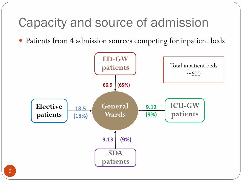
Capacity and source of admission Patients from 4 admission sources competing for inpatient beds

Total inpatient beds ~600

5

General Wards

ED-GW patients

ICU-GW patients

SDA patients

Elective patients

66.9 (65%)

18.5 (18%)

9.13 (9%)

9.12 (9%)

Key performance measures Waiting time for admission to ward (Jan 08 – Jun 09) Waiting time = admission time – bed request time Average: 2.82 hour 6.52% of ED-GW patients wait more than 6 hours to get a bed 6-hour service level MOH cares

Quality- and Efficiency-Driven (QED) Average waiting time = 2.3% (average service time) Average bed utilization = 90%

6

Time dependency Waiting time depends on patient’s bed request time Can we stabilize?

7

Time-varying bed request rate

8

ED-GW patient’s bed request rate (red curve) depends on arrival rate to ED (blue curve)

Learning from call center research?

9

Zohar Feldman, Avishai Mandelbaum, William A. Massey and Ward Whitt, Management Sciences, 2008 Staffing of Time-Varying Queues to Achieve Time-Stable

Performance

Yunan Liu and Ward Whitt, 2012 Stabilizing customer abandonment in many-server

queues with time-varying arrivals

Mismatch between demand and supply of beds Jan 08 – Jun 09

10

Discharge policy

11

Discharge timing affects the waiting time Early discharge policy Moving the discharge time a few hours earlier in the day

The hospital implemented early discharge policy since July 2009 Study two periods of data Jan 2008 to Jun 2009 (Period 1)

13% before noon Jan 2010 to Dec 2010 (Period 2)

26% before noon

Waiting time for ED-GW patients

12

1st period 2nd period

Average waiting time 2.82 h 2.77 h

6-hour service level 6.52% 5.13%

Challenges

13

Does the modest improvement come from the early discharge? Changing operating environment Both arrival volume and capacity increases during 2008 to 2010 Bed occupancy rate (BOR) reduces in the Period 2

Period 1: 90.3% Period 2: 87.6%

More importantly, is there any operational policy that can

stabilize the waiting time?

Need a model to help

Part II: A stochastic model

14

Model Hospital Inpatient Operations: Mathematical Models and

Managerial Insights, submitted

Joint work with Mabel Chou, Ding Ding, and Joe Sim

A multiclass, multi-server pool system

15

Time-varying arrival rates

16

Specialty distribution

17

Key modeling components

18

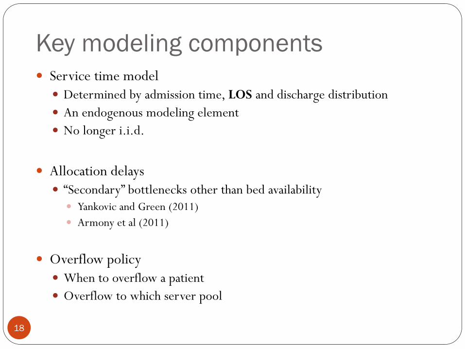
Service time model Determined by admission time, LOS and discharge distribution An endogenous modeling element No longer i.i.d.

Allocation delays “Secondary” bottlenecks other than bed availability Yankovic and Green (2011) Armony et al (2011)

Overflow policy When to overflow a patient Overflow to which server pool

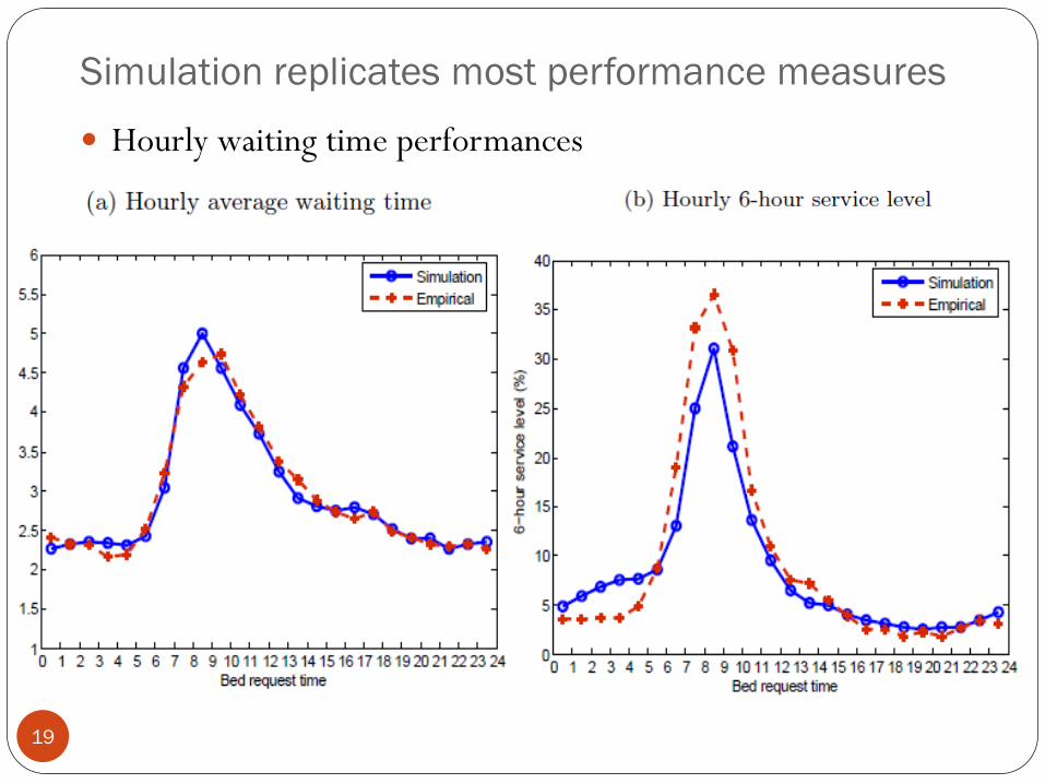
Simulation replicates most performance measures

Hourly waiting time performances

19

Time-dependent queue length

20

0 2 4 6 8 10 12 14 16 18 200

0.05

0.1

0.15

0.2

0.25Period 1Period 2

Length of Stay (LOS) = Discharge day – Adm day

Service times are endogenous Service time model Service time = Discharge time – Admission time = LOS + Dis hour – Adm hour

LOS distribution Average is ~ 5 days Depend on admission source and specialty AM- and PM- dependent for ED-GW patients

21

Verify the service time model Service time model Service time = LOS + Discharge hour – Adm hour Matching empirical (a) Empirical (Armony et al 2011) (b) Simulation output

0 2 4 6 8 10 12 14 16 18 200

0.02

0.04

0.06

0.08

0.1

0.12

0.14

0.16

0.18histogram of service time

0 2 4 6 8 10 12 14 16 18 200

0.02

0.04

0.06

0.08

0.1

0.12

0.14

0.16

0.18histogram of service time

22

Pre- and post-allocation delays Patient experiences additional delays upon arrival and when a

bed is allocated Pre-allocation delay BMU search/negotiate for beds

Post-allocation delay Delays in ED discharge Delays in the transportation Delays in ward admission

Must model allocation delays If not, hourly queue length does not match (right figure) 23

Time-dependent allocation delays The mean of allocation delay depends on when it is initiated Use log-normal distribution Pre-allocation delay

Overflow policy

25

When a patient’s waiting time exceeds certain threshold, the patient can be overflowed to a “wrong” ward Beds are partially flexible Overflow wards have certain priority

Cluster 1st Overflow 2nd Overflow 3rd Overflow Medicine Other Med Surgery/OG Ortho Surgery Other Surg Ortho /OG Medicine Ortho Other Ortho Surgery Medicine

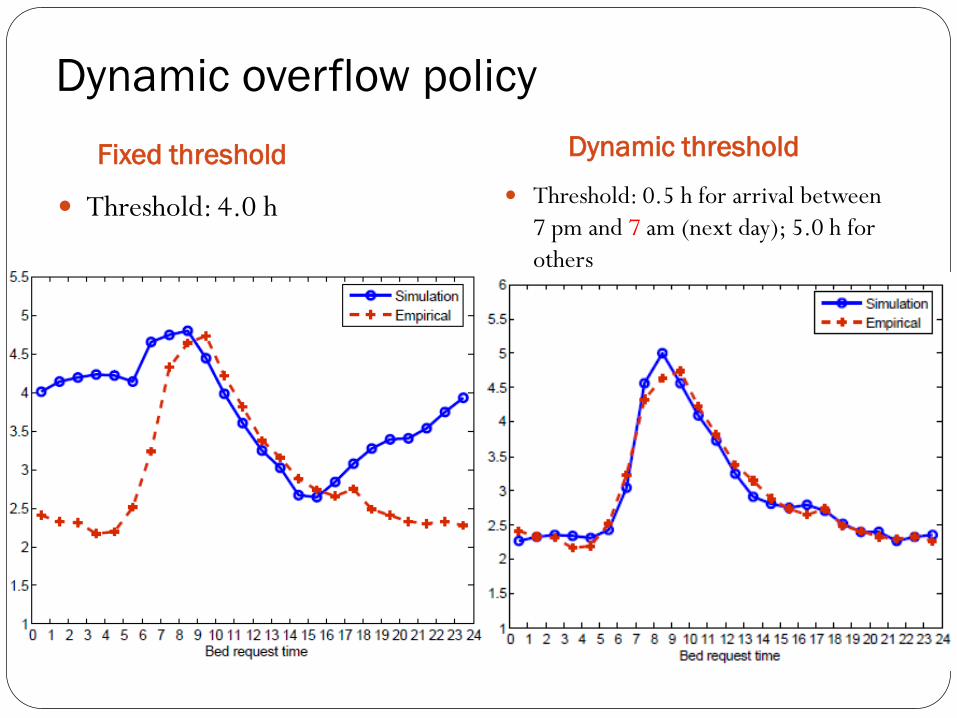
Dynamic overflow policy Fixed threshold

Threshold: 4.0 h

Dynamic threshold

Threshold: 0.5 h for arrival between 7 pm and 7 am (next day); 5.0 h for others

Part III: Analytical analysis

27

Two-time scale method to predict time-dependent performance measures

Two-time scale

28

Discrete queue Average LOS and daily arrival rate determine , and thus

performances at mid-night (daily level)

Time-varying performance The arrival rate pattern, discharge timing, and allocation delay

distribution determine the hour-of-day behavior

A simplified model

29

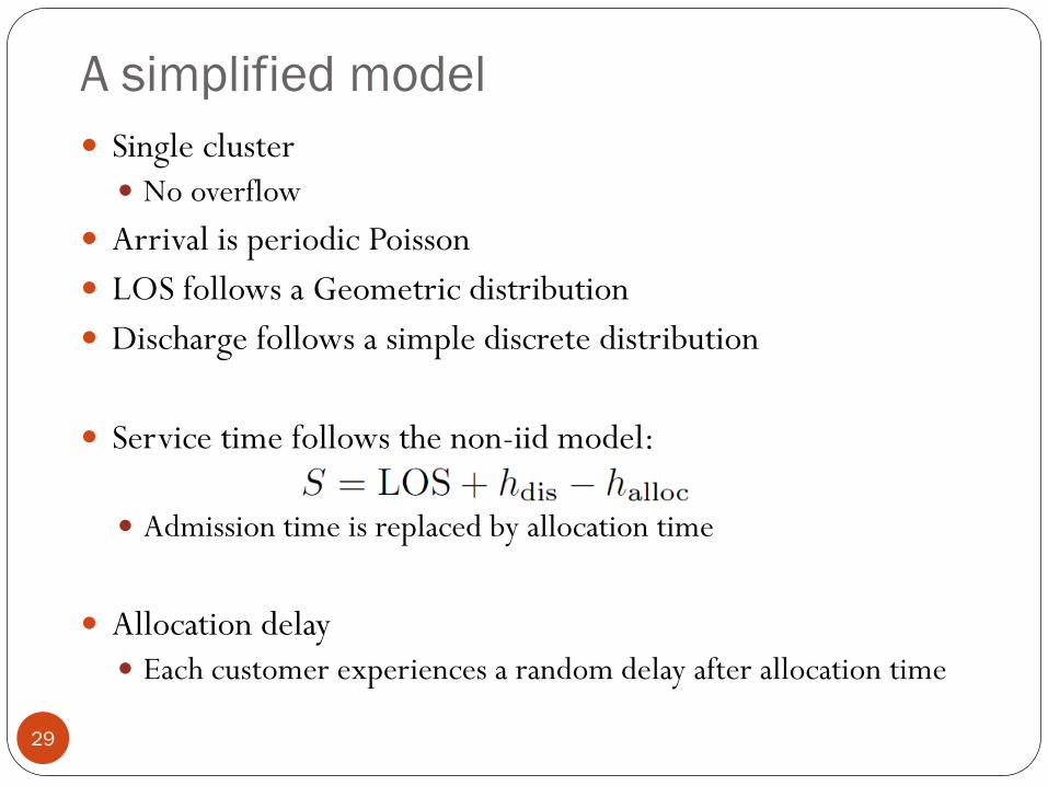
Single cluster No overflow

Arrival is periodic Poisson LOS follows a Geometric distribution Discharge follows a simple discrete distribution

Service time follows the non-iid model:

Admission time is replaced by allocation time

Allocation delay Each customer experiences a random delay after allocation time

Predict the time-dependent average queue length

30

Decompose the queue length into two parts Queue for beds: patients who are waiting for a bed

Alloc-delay queue: patients who are allocated with beds and are

experiencing the alloc-delay

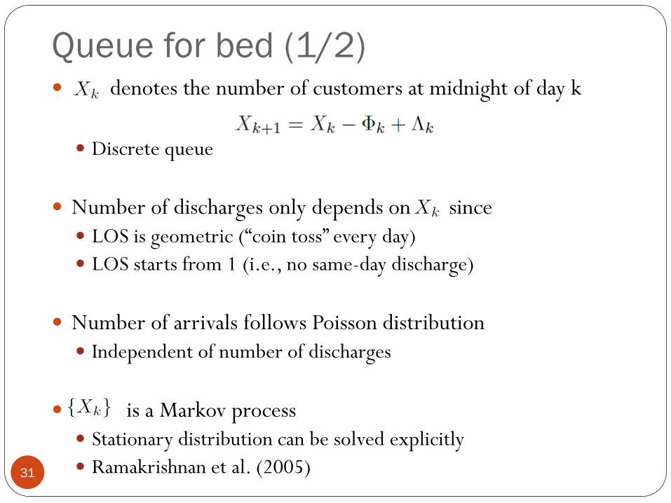
Queue for bed (1/2) denotes the number of customers at midnight of day k

Discrete queue

Number of discharges only depends on since LOS is geometric (“coin toss” every day) LOS starts from 1 (i.e., no same-day discharge)

Number of arrivals follows Poisson distribution Independent of number of discharges

is a Markov process Stationary distribution can be solved explicitly Ramakrishnan et al. (2005) 31

Queue for bed (2/2) Using the stationary distribution of The average number of customers in system and the average queue

length can be obtained for any time point Average number of customer in system can be solved in a fluid way

Powell et al. (2012)

Queue length needs to be obtained from the distribution of

number of customers in system at each time point Conditioning on is a convolution between arrival (Poisson r.v.) and

discharge (Binomial r.v. depends on the value of ) till t

32

Related work

33

E. S. Powell, R. K. Khare, A. K. Venkatesh, B. D. Van Roo, J. G. Adams, and G. Reinhardt, The Journal of Emergency Medicine, 2012 The relationship between inpatient discharge timing and

emergency department boarding

Affiliations: Department of Emergency Medicine, Northwestern University; Harvard Affiliated Emergency Medicine Residency, Brigham and Women’s Hospital–Massachusetts General Hospital, …

Alloc-delay queue

34

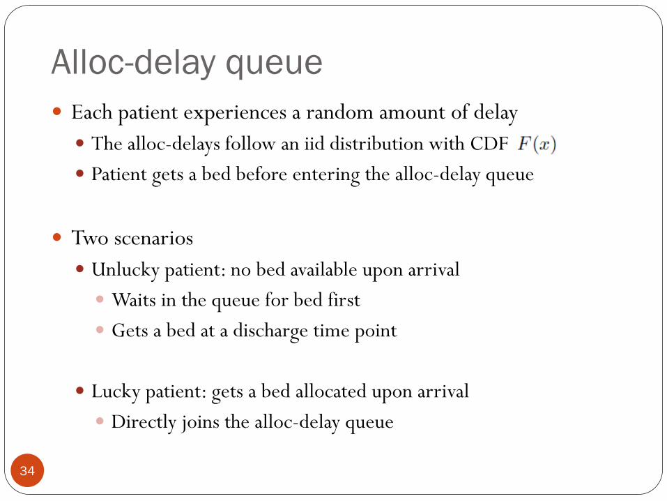
Each patient experiences a random amount of delay The alloc-delays follow an iid distribution with CDF Patient gets a bed before entering the alloc-delay queue

Two scenarios Unlucky patient: no bed available upon arrival Waits in the queue for bed first Gets a bed at a discharge time point

Lucky patient: gets a bed allocated upon arrival Directly joins the alloc-delay queue

Unlucky patients

35

Suppose discharges occur at The mean number of admissions at each discharge point can be

calculated from , arrivals and discharges

Given the mean number of admissions Mean number of customers in the alloc-delay queue after s hours is

Lucky patients

36

The effective admission process (bed-allocation process) is non-homogeneous Poisson The probability of an arriving patient being lucky or unlucky is

independent of the arrival itself The effective admission rate can be calculated from , arrivals

and discharges

Consider the alloc-delay queue as an infinite-server queue Service time is the allocation delay The effective admission process constitutes the arrival Infinite-server queue theory (Eick - 1993):

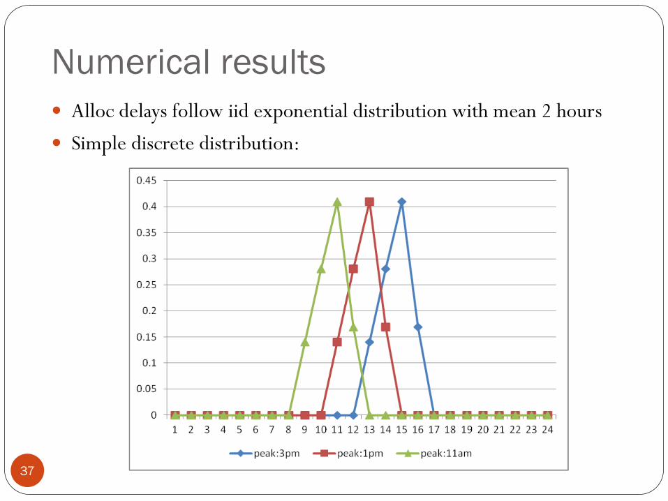
Numerical results Alloc delays follow iid exponential distribution with mean 2 hours

Simple discrete distribution:

37

Numerical results

38

Avg queue length

Insights from the simplified model

39

The average number of customers in the system remain the same in scenarios with and without allocation delays

Challenging to predicting the hourly queue length Necessary to model allocation delays Slower drop in the queue length after 2pm

Early discharge helps stabilize the hourly queue length

Shift the Period 1 discharge curve

40

Using constant-mean allocation delay Avg queue length Avg waiting time

Part IV: Managerial insights

41

Whether early discharge policy is beneficial or not

What-if analysis

Simulation results Simulation shows NUH early discharge policy has little improvement

(a) hourly avg. waiting time (b) 6-hour service level

42

Aggressive early discharge policy

43

Aggressive early discharge + smooth allocation delay

44

Waiting time performances can be stabilized (a) hourly avg. waiting time (b) 6-hour service level

Only use aggressive early discharge

45

Cannot be stabilized (a) hourly avg. waiting time (b) 6-hour service level

Only smooth the allocation delays

46

Assuming allocation delay has a constant mean (a) hourly avg. waiting time (b) 6-hour service level

Impact of capacity increase

47

10% reduction in utilization, plus assuming allocation delay has a constant mean (a) hourly avg. waiting time (b) 6-hour service level

Summary Conduct an empirical study of patient flow of the entire

inpatient department

Build and calibrate a stochastic model to evaluate the impact of discharge distribution on waiting for admission to ward

Analyze a simplified version of the stochastic model using a two-time scale approach

Achieve stable waiting time by aggressive early discharge + smooth allocation delay

48

49

Questions?

Limitations

50

Simulation cannot fully calibrate with the overflow rate Bed class (A, B, C) Gender mismatch Hospital acquired infections Example: a female Surg patient has to be overflowed to a Med ward, since

the only available Surg beds are for males

Day-of-week phenomenon Admission and discharge both depends on the day of week LOS depends on admission day Performances (BOR, waiting time) varies among days

51

Appendix

Simulation replicates most performance measures

Hourly waiting time performances

52

Average queue length (simulation result)

53

Average waiting time for each specialty

54

Renal patients have longest average waiting time

6-hour service level for each specialty

55

Cardio and Oncology patients show significant improvement in the 6-hour service level

Overflow rate

56

Overall overflow rate reduces in Period 2

Background One of the major hospitals in Singapore Around 1,000 beds in total

38 inpatient wards We focus on 21 general wards ICU, ISO, pediatric wards are excluded Wards are dedicated to one specialty or shared by two and more

specialties

Serving around 90,000 patients annually Data from 2008 to 2010

57

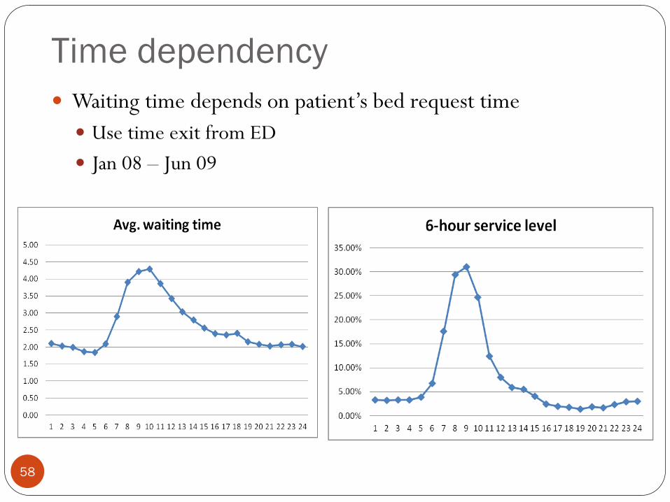
Time dependency Waiting time depends on patient’s bed request time Use time exit from ED Jan 08 – Jun 09

58

Waiting time for ED patients (using MOH definition)

59

(a) hourly avg. waiting time (b) hourly 6-hour service level

1st period 2nd period

Average waiting time 2.50 h 2.44 h

6-hour service level 5.24% 3.90%

Histogram of waiting time (MOH definition)

60

Histogram of service time Resolution of 1 hour Period 1 Period 2

0 2 4 6 8 10 12 14 16 18 200

0.05

0.1

0.15

0.2

0.25histogram of service timerevised LOS distribution

0 2 4 6 8 10 12 14 16 18 200

0.05

0.1

0.15

0.2

0.25histogram of service timerevised LOS distribution

Log-normal fit for LOS distribution

62

Relation between residual, Tadm, and Tdis Residual

Alternative service time model (1/2)

64

S = Tdis – Tadm S denote service time (in unit of day)

Tadm denote the admission time, Tdis denote the discharge time

Residual = S – floor(S)

histogram (right fig)

In the alternative model Generate the integer part floor(S) from empirical distribution Independently generate the residual from another empirical distribution

0 0.1 0.2 0.3 0.4 0.5 0.6 0.7 0.8 0.9 10

0.01

0.02

0.03

0.04

0.05

0.06

0.07

0.08

0.09Period 1Period 2

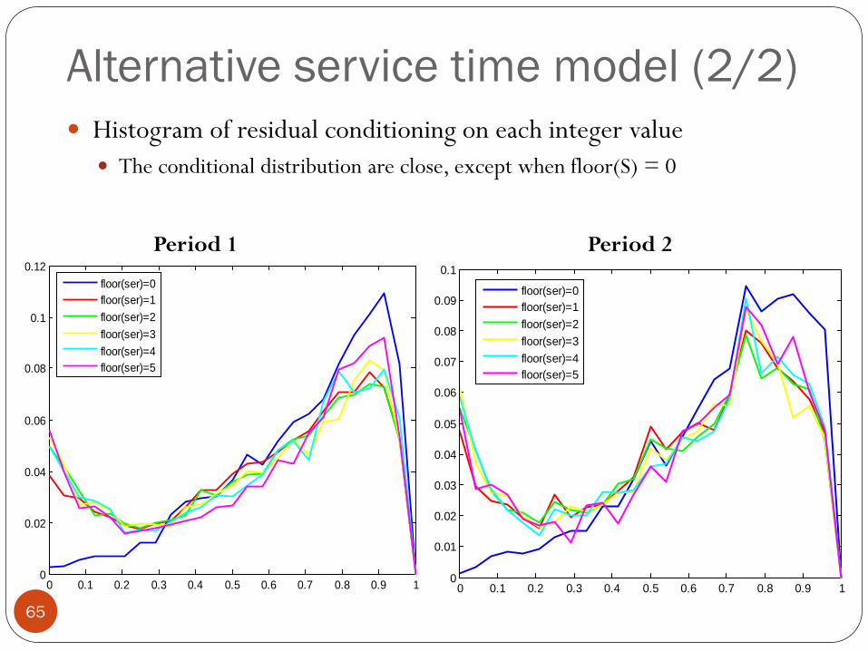
Alternative service time model (2/2)

65

Histogram of residual conditioning on each integer value The conditional distribution are close, except when floor(S) = 0

Period 1 Period 2

0 0.1 0.2 0.3 0.4 0.5 0.6 0.7 0.8 0.9 10

0.02

0.04

0.06

0.08

0.1

0.12floor(ser)=0floor(ser)=1floor(ser)=2floor(ser)=3floor(ser)=4floor(ser)=5

0 0.1 0.2 0.3 0.4 0.5 0.6 0.7 0.8 0.9 10

0.01

0.02

0.03

0.04

0.05

0.06

0.07

0.08

0.09

0.1

floor(ser)=0floor(ser)=1floor(ser)=2floor(ser)=3floor(ser)=4floor(ser)=5

Alternative service time model If directly generating service time Discharge distribution does not match Avg. waiting time does not match

66

Stochastic network models

67

Multiclass, multi-server pools with some flexible pools 30 ~ 60 servers in each pool 15 server pools

Typical BOR is 86% ~ 93%

Periodic arrival processes

Long service times = several arrival periods Average LOS = 5 days

Waiting time is a small fraction of service time Average waiting time = 2.5 hours = 1/48 average LOS

Must overflow in a fraction of the service time

Simulation model Using 9 cluster of patients and 15 server pools

Utilization (Sim): 90.5%; (empirical): 88.0% We did not catch gender/ bed class /sub-specialty mismatch in simulation

4 types of arrivals for each cluster ED-GW EL ICU-GW SDA Use empirical arrival rate and service time for each type of patients

68

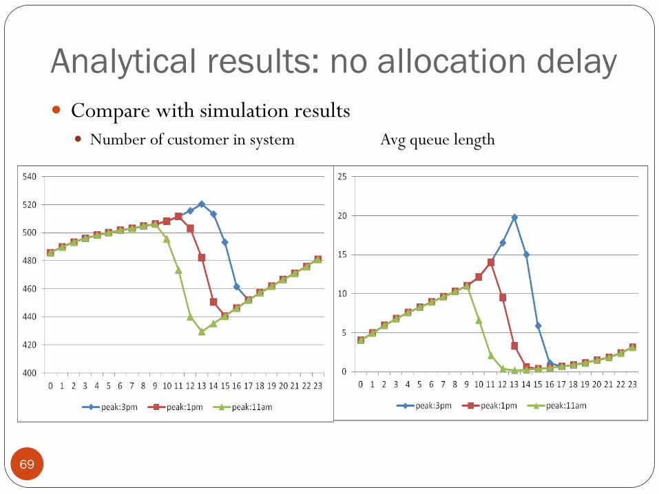
Analytical results: no allocation delay

69

Compare with simulation results Number of customer in system Avg queue length

A stochastic model Multi-class, multi-server pool system Each server pool is either dedicated to one class of customer or

flexible to serve two and more classes of customers

Periodic arrival 4 types of arrival (ED-GW, Elective, ICU-GW, SDA) for each

specialty

A novel service time model

And other key components

70

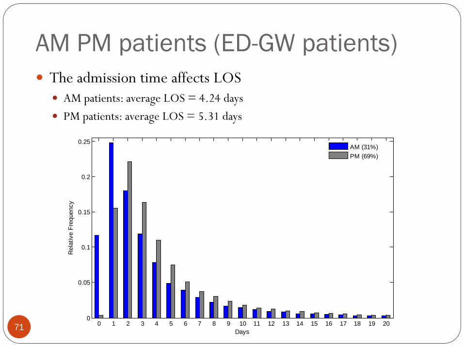
AM PM patients (ED-GW patients)

71

The admission time affects LOS AM patients: average LOS = 4.24 days PM patients: average LOS = 5.31 days

0 1 2 3 4 5 6 7 8 9 10 11 12 13 14 15 16 17 18 19 200

0.05

0.1

0.15

0.2

0.25

Days

Rel

ativ

e Fr

eque

ncy

AM (31%) PM (69%)